How does currency diversification explain banks' leverage ...

How does currency diversification explain banks’

leverage procyclicality?∗

Justine Pedrono†

April 2018

abstract:

The amplitude and dynamics of the leverage procyclicality are heterogeneous acrossbanks and across countries. This paper explores whether currency diversification ofbank’s balance sheet is a factor of this observed heterogeneity. The theoretical modelpredicts that the impact of currency diversification on bank’s leverage procyclicalitydepends on the relative performance of economies, the global business cycle and theexchange rate regime. Using novel micro data on banks located in France, I show thatthe pre-crisis currency diversification of banks increases banks’ leverage procyclicalityduring the 2008-2009 crisis. Focusing on the foreign exchange rate impact, namely thevaluation effect of currency diversification, my results suggest that it had a negative ef-fect on leverage procyclicality during this period. These findings confirm the theoreticalprediction and draw attention to the specific role of balance sheet currency diversifica-tion in financial stability risk.

JEL classification: F36, G15, G21, G32

Keywords: bank, financial intermediary, leverage, procyclicality, currency, diversifi-cation, Value-at-Risk, exchange rate.

∗The views expressed here are those of the author and do not necessarily represent those of theBanque de France. This paper builds on a previous working paper, which circulated under the title:”Banking leverage procyclicality: a theoretical model introducing currency diversification”. I am verygrateful to Mohamed Belhaj, Agnes Benassy Quere, Benjamin Carton, Nicolas Coeurdacier, Olivier DeBandt, Reint Gropp, Dirk Krueger, Patrick Pintus, Hyun Song Shin, Helene Rey as well as participantsat the ECB’s Sintra forum (2015), and seminar participants at the Aix Marseille School of Economicsand the Paris School of Economics for very helpful comments. I am also indebted to the Aix MarseilleSchool of Economics for financial and technical support provided during my PhD.†ACPR Banque de France, Aix-Marseille Univ., CNRS, EHESS, Centrale Marseille, AMSE.

E-mail:[email protected]

1

1 Introduction

The procyclical dimension of banks’ leverage defined by Shin [2012] and Adrian and

Shin [2014] has been a subject of keen interest, especially in the wake of the crisis. In

this framework, banks’ leverage is the ratio of total assets to equity and leverage pro-

cyclicality refers to the cyclical variations of their leverage according to the value of their

assets that are used as collateral. The higher the collateral value, the larger the banks’

capacity to raise funds and extend leverage. Extending their leverage, banks strengthen

the value of assets and create an endogenous mechanism similar to the financial acceler-

ator ([Danielsson. et al., 2012]). Because of the amplification of booms and bursts, the

procyclicality of banking activities is a major source of economic instability: the identi-

fication of the determinants of leverage procyclicality is then a matter of general interest.

Focusing on US, European and Canadian banks, Adrian and Shin [2008], Kalemli-

Ozcan et al. [2012], Baglioni et al. [2013], Damar et al. [2013] confirm the general pro-

cyclicality of banks’ leverage: there is a strong and positive correlation between the

growth rate of assets and the growth rate of leverage. However, their results raise the

question of heterogeneity in leverage procyclicality as banks located in different geo-

graphic areas show different level of leverage procyclicality. Especially, Kalemli-Ozcan

et al. [2012] show that European banks exhibit less procyclical leverage than their Amer-

ican counterpart, leaving the source of this heterogeneity unexplained. Acknowledging

the global architecture of international banking, Bruno and Shin [2015] define a gen-

eral framework with a global and a regional representative bank. While this framework

provides a first insight on the role of international banking by capturing the aggregate

leverage procyclicality as a function of a common risk factor, it does not explain the

observed heterogeneity mentioned in Kalemli-Ozcan et al. [2012] either.

Milesi-Ferretti et al. [2011] confirm high heterogeneity in the impact of the crisis and

1

suggest that the extent of international financial integration and banking involvement

could play a role. Banks having different exposures to different markets and risks may

then exhibit distinct leverage procyclicality. Comparing Americain and euro area (EA)

banks, Baba et al. [2009] highlight a transatlantic asymmetry in international banking:

assets of EA banks denominated in US dollars account for about $4.5 trillion in 2008,

while the assets of US banks denominated in European currencies only amount to $1.5

trillion. This specific international involvement of European banks makes them crucial

intermediates in cross-border credit (Cerutti et al. [2017]). To some extent, it could also

explain the observed heterogeneity in their cyclical variations of leverage. Focusing on

aggregate data on European banks, Krogstrup and Tille [2017] introduce the hetero-

geneity in banks’ balance sheet as an additional variable to explain the heterogeneous

responses to global risk factor. They show that foreign currency mismatch in banks’

balance sheet has a significant impact on the responses to global shock. Using microdata

for emerging markets, Baskaya et al. [2017] show that banks’ funding heterogeneity is

the main driver of aggregate credit growth.

This paper contributes to the recent literature which focuses on banking hetero-

geneity by analyzing the impact of bank’s currency diversification on bank’s leverage

procyclicality. Currency diversification is the share of assets (or liabilities) denominated

in one specific currency. By identifying the currency denomination of assets and liabili-

ties, I pay attention to the fact that not all foreign currencies are alike, especially when it

is associated to financial stability risk (Krogstrup and Tille [2016]). The contributions of

this paper are twofold. The first contribution is theoretical while the second is empirical.

The first contribution can be found in the capacity of the model to depict two main

channels of international banking, namely the risk diversification and the valuation ef-

fect of foreign exchange rate. In this paper, I use a contract model a la Holmstrom

2

and Tirole [1997] between the bank and the creditor to micro-found the Value-at-Risk

(VaR) rule. The VaR rule stipulates that banks maintain a stable probability of fail-

ure, implying an increase in leverage when the economy is booming and a decrease in

leverage when the economy is bursting. Banks’ leverage is procyclical due to the VaR

rule. Because the VaR measures the tail risk of banks, it is also determinant for banks’

systemic risk and relevant for economic stability.1 The main difference with Adrian and

Shin [2014] where a contract model is also used to micro-found the VaR is the distri-

bution of bank’s asset returns. Here, the distribution of bank’s portfolio depends on a

mixture of distributions between the different asset returns and is especially compatible

with the global involvement of banks. It allows to capture and depict two main channels

of international banking, namely the diversification of risk and the valuation effect due

to foreign exchange rate. My model also differs from the general theoretical framework

presented in Bruno and Shin [2015] for three reasons. First, it micro-founds the VaR

instead of applying it to the cross-border network. Second, it captures the currency

diversification of banks and addresses more globally the international banking issue by

fitting the stylized facts on European banks detailed above.2 Third, it makes the ex-

change rate fluctuations endogenous to relative economic performances.

I focus in this paper on the diversification between domestic and foreign assets but

the simplicity of the framework may allow researchers to use it for different purposes,

like a diversification between different sectors or different types of assets. Regarding

currency diversification, the model shows that introducing foreign asset and debt in

foreign currency does not remove the micro-foundation of the VaR but it impacts the

1As supported by Benoit et al. [2013], the systemic risk of banks captured by ∆CoV aR is proportionalto the VaR, under certain conditions.

2The model defined in Bruno and Shin [2015] includes an exogenous exchange rate, a global bank, aregional bank, and a local firm. Both the global and the regional bank carry out their financial operationsin foreign currency, therefore there is no currency diversification in their balance sheets. In contrast, thelocal firm invests in local currency and raises debt from the regional bank in foreign currency. Thus,currency risk is only borne by the local firm and banks’ portfolio only consists of one common risk factor.

3

adjustment of leverage, i.e the leverage procyclicality, through the tail risk of banks.

When the foreign economic condition is more volatile than the domestic one under a

fixed exchange rate regime, leverage becomes more procyclical with currency diversifi-

cation than without. Similarly, currency diversification reduces leverage procyclicality

when the foreign economic condition is less volatile than the domestic one. Valuation

effect aside, the generalized conclusions of the model also support previous results from

Kwok and Reeb [2000] which visit the upstream downstream hypothesis of international-

ization. A floating exchange rate regime then introduces a valuation effect on converted

asset and debt which impacts leverage adjustment. Assuming that currency appreciates

when its economy outperforms others, a floating exchange rate decreases the tail risk

and expands the bank’s capacity to raise funds. Compared to a fixed exchange rate

regime, valuation effect increases procyclicality during booms and decreases it during

burst. This model then implies two distinct components explaining the heterogeneous

leverage procyclicality: a diversification of risks between the two countries and a valua-

tion effect due to floating exchange rate regime.

The second contribution is an empirical one. Using novel micro data on banks, this

paper is then the first one to measure currency diversification of banks balance sheet

and its implication on leverage procyclicality. These granular data allow me to dig

deeper compared to Krogstrup and Tille [2017] and to measure the two components of

heterogeneous leverage procyclicality. By focusing on both the leverage procyclicality

of banks and on the currency diversification of their balance sheet, this paper not only

captures activities associated to foreign exposures but also purely domestic activities. It

then provides a complete picture of banks’ activities (domestic and foreign) and draws

attention to the specific role of balance sheet currency diversification in financial sta-

bility risk. Following theoretical predictions, banks with exposures to the US and the

US dollar are supposed to show different leverage procyclicality during the 2008-2009

4

crisis than banks with low diversification. Considering banks located in France and the

2008-2009 crisis coming from the US, an increase in leverage procyclicality due to cur-

rency diversification is then to be expected during this period. Focusing on the valuation

effect of currency diversification; however, one can expect that it had a negative impact

on leverage procyclicality because of the floating exchange regime. Especially, did the

pre-crisis currency diversification of assets in 2007 affect the large adjustment of banks’

balance sheet during the crisis between 2008 and 2009? If it is the case, how did it affect

it? My results yield supporting evidences to my theoretical predictions: currency diver-

sification had increased leverage procyclicality during the 2008-2009 crisis; however, the

valuation effect itself had a negative impact on leverage procyclicality.

The rest of the paper is organized as follows. Section 2 introduces the theoretical

model while section 3 develops the quantitative analysis using innovative micro-data.

Section 4 concludes.

2 Model

2.1 Setting

The model is based on a representative bank’s balance sheet. The bank invests in assets

and raises funds from its creditor. Here, though, there are two currency denominations

for assets and debts, corresponding to two different countries (domestic and foreign).

The economic state of nature corresponding to each economy is known publicly and

determine the distribution of asset returns. There are two periods T=0,1. The state of

nature and the distribution of returns are known at T=0.

The representative bank is domestic in the sense that its equity and its balance sheet

5

are in domestic currency. The bank is risk neutral and equity E is exogenous.3 The

second agent is the creditor of the bank, generally a Money Market Fund or another

investment bank. The creditor lends money to the bank in both currencies (domestic

and foreign). The creditor is also risk neutral. The exchange rate S is defined as the

number of domestic units per unit of foreign currency.

At T=0, the bank raises funds backed by collateral in domestic and foreign cur-

rency (A and A?, respectively). Total assets expressed in domestic currency are equal

to A+SA?. I denote by a the share of assets in domestic currency and (1−a) the share

of assets in foreign currency. a will vary depending on S. In this section, I consider S

as fixed. Section 2.4 covers the case of a flexible exchange rate regime. Funds are in

domestic and in foreign currency (D and D?, respectively). Thus, total funding from the

creditor expressed in domestic currency is equal to D + SD?. This debt is defaultable,

implying that the creditor receives a defaultable debt claim at T=0.

At T=1, the bank receives a total expected return from its investments a(1+r)+(1−

a)(1 + r?), where r and r? are the expected returns from the domestic and the foreign

asset, respectively. Returns depend on the state of nature specific to each currency area,

θ and θ?, respectively. θ and θ? are known publicly from T=0 and they do not change

between the two periods. At T=1, the bank also reimburses its domestic and foreign

debts, D and SD? respectively. As θ and θ? are known for the two periods, there is

no macroeconomic risk. It is assumed that D > D and SD? > SD? to remunerate the

creditor for the default risk.

The bank’s balance sheets at each period are given in table 1 where E is the equity

at notional value.

3An exogenous equity is in line with the theory of procyclical leverage put forward by Shin.

6

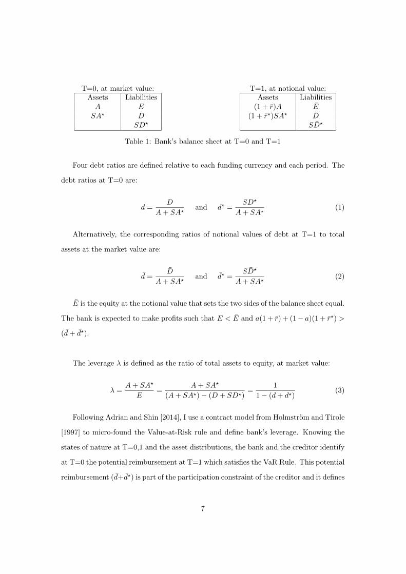
T=0, at market value:Assets LiabilitiesA ESA? D

SD?

T=1, at notional value:Assets Liabilities

(1 + r)A E(1 + r?)SA? D

SD?

Table 1: Bank’s balance sheet at T=0 and T=1

Four debt ratios are defined relative to each funding currency and each period. The

debt ratios at T=0 are:

d =D

A+ SA?and d? =

SD?

A+ SA?(1)

Alternatively, the corresponding ratios of notional values of debt at T=1 to total

assets at the market value are:

d =D

A+ SA?and d? =

SD?

A+ SA?(2)

E is the equity at the notional value that sets the two sides of the balance sheet equal.

The bank is expected to make profits such that E < E and a(1 + r) + (1− a)(1 + r?) >

(d+ d?).

The leverage λ is defined as the ratio of total assets to equity, at market value:

λ =A+ SA?

E=

A+ SA?

(A+ SA?)− (D + SD?)=

1

1− (d+ d?)(3)

Following Adrian and Shin [2014], I use a contract model from Holmstrom and Tirole

[1997] to micro-found the Value-at-Risk rule and define bank’s leverage. Knowing the

states of nature at T=0,1 and the asset distributions, the bank and the creditor identify

at T=0 the potential reimbursement at T=1 which satisfies the VaR Rule. This potential

reimbursement (d+d?) is part of the participation constraint of the creditor and it defines

7

the total debt the creditor is willing to lend to the bank at T=0 and the leverage. The

rest of the section is devoted to the development of the contract model and the detailed

theoretical results.

2.2 Investment strategy

To introduce the contract model between the creditor and the bank as in Holmstrom

and Tirole [1997], the bank makes an indivisible choice between two types of portfolio:

a good portfolio indexed by H,H? and a less good portfolio L,L?. Each portfolio is

composed of an asset in domestic currency and an asset in foreign currency, where an as-

terisk indicates foreign assets. The weight of each type of asset is given by a and (1−a).

The portfolio’s distribution comes from a mixture distribution of the two asset return

distributions. Assuming that each asset return follows a General Extreme Value (GEV)

distribution, the portfolio’s return is also defined by a GEV distribution. The first port-

folio H,H? is a ”good” portfolio with a total expected return of [arH + (1 − a)rH? ],

where rH denotes the expected return from the good domestic asset and rH? the ex-

pected return from the good foreign asset. The second portfolio L,L? is not as good.

Its total expected return [arL + (1 − a)rL? ] is reduced through a parameter k (k > 0)

and its volatility is increased by a parameter m (m > 1) compared to the good portfolio.

The Cumulative Distribution Functions (CDF) of portfolio return when the bank

8

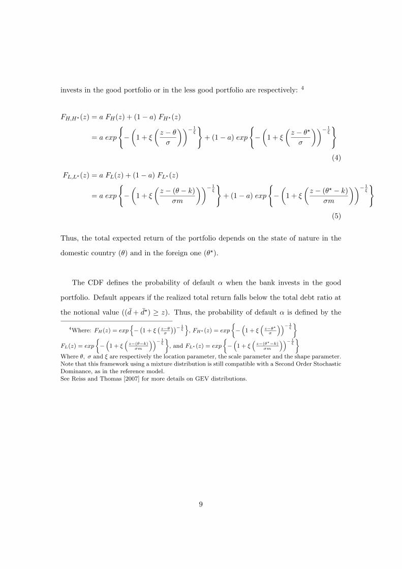
invests in the good portfolio or in the less good portfolio are respectively: 4

FH,H?(z) = a FH(z) + (1− a) FH?(z)

= a exp

−(

1 + ξ

(z − θσ

))− 1ξ

+ (1− a) exp

−(

1 + ξ

(z − θ?

σ

))− 1ξ

(4)

FL,L?(z) = a FL(z) + (1− a) FL?(z)

= a exp

−(

1 + ξ

(z − (θ − k)

σm

))− 1ξ

+ (1− a) exp

−(

1 + ξ

(z − (θ? − k)

σm

))− 1ξ

(5)

Thus, the total expected return of the portfolio depends on the state of nature in the

domestic country (θ) and in the foreign one (θ?).

The CDF defines the probability of default α when the bank invests in the good

portfolio. Default appears if the realized total return falls below the total debt ratio at

the notional value ((d + d?) ≥ z). Thus, the probability of default α is defined by the

4Where: FH(z) = exp−(1 + ξ

(z−θσ

))− 1ξ

, FH?(z) = exp

−(

1 + ξ(z−θ?σ

))− 1ξ

FL(z) = exp

−(

1 + ξ(z−(θ−k)σm

))− 1ξ

, and FL?(z) = exp

−(

1 + ξ(z−(θ?−k)

σm

))− 1ξ

Where θ, σ and ξ are respectively the location parameter, the scale parameter and the shape parameter.Note that this framework using a mixture distribution is still compatible with a Second Order StochasticDominance, as in the reference model.See Reiss and Thomas [2007] for more details on GEV distributions.

9

cumulative distribution function such that:5

α(d+ d?) = FH,H?(d+ d?)

= a exp

−(

1 + ξ

((d+ d?)− θ

σ

))− 1ξ

+ (1− a) exp

−(

1 + ξ

((d+ d?)− θ?

σ

))− 1ξ

(6)

Since the creditor is uninsured, he/she holds a defaultable debt claim with respect

to the funds lent to the bank at T=0. According to Merton [1974], the value of this

defaultable debt claim with strike price (D+SD?) can be divided into two components:

cash (D + SD?) and a short position on a put option π. Thereby, the value of a

defaultable debt claim is lower than its expected payoff (D+SD?) because of its induced

risk. Since the risk differs between the two types of portfolio, the put option is specific

to each investment choice. If the bank invests in the good portfolio, the following put

option price is given by:6

πH,H?(D + S.D?, A+ SA?) = (A+ SA?).πH,H?(d+ d?, 1) ≡ (A+ SA?).πH,H?(d+ d?)

If the bank invests in the bad portfolio, the price of the put option is:

πL,L?(D + S.D?, A+ SA?) = (A+ SA?).πL,L?(d+ d?, 1) ≡ (A+ SA?).πL,L?(d+ d?)

5Alternatively, the probability of default when the bank invests in the ”less good” portfolio can bedefined through FL,L?(d + d?). However, I focus on the good portfolio since the contract between thebank and its creditor leads to this portfolio in section 3.

6The price of the put option depends on the total amount reimbursed at the end of the period -D + S.D? - and on the total value of assets A + SA?. Assuming that there is a constant returns toscale of option price because of competitive markets, the value of the option on total portfolio A+ SA?

with strike priceD + SD? can be recover by bundling together A + SA? options on one dollar’s worthof portfolio with strike price (D + SD?)/(A+ SA?).

10

2.3 Incentive constraints

The creditor of the bank is risk neutral. He maximizes his utility UC defined as his total

net expected payoff. His net expected payoff is the difference between the value of his

defaultable debt claim and the total funds provided to the bank. If the bank invests in

the good portfolio, the net expected payoff is given by:

UCH,H?(A+ SA?) = (A+ SA?)[(d+ d?)− πH,H?(d+ d?)− (d+ d?)

](7)

The requirement that utility is equal to or higher than 0 provides the first Participa-

tion Compatibility (PC) constraint of the creditor. This constraint binds in the optimal

contract:

0 ≤ (d+ d?)− πH,H?(d+ d?)− (d+ d?) (8)

(d+ d?) = (d+ d?)− πH,H?(d+ d?) (9)

Similarly for an investment in the bad portfolio:

(d+ d?) = (d+ d?)− πL,L?(d+ d?) (10)

The PC constraint (9) defines the total debt ratio at market value relative to the total

debt ratio at notional value. The latter should be large enough to form an incentive

for the creditor to participate. The higher the reimbursement offered by the bank, the

more the creditor is tempted to lend money at T=0.

The bank is risk neutral and maximizes its expected utility UB defined as its total

net expected payoff. In this framework, returns come from assets both in domestic and

in foreign currency. Thus the net expected payoff when the bank invests in the good

11

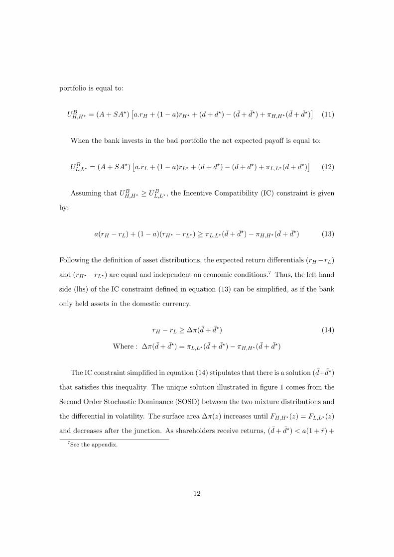
portfolio is equal to:

UBH,H? = (A+ SA?)[a.rH + (1− a)rH? + (d+ d?)− (d+ d?) + πH,H?(d+ d?)

](11)

When the bank invests in the bad portfolio the net expected payoff is equal to:

UBL,L? = (A+ SA?)[a.rL + (1− a)rL? + (d+ d?)− (d+ d?) + πL,L?(d+ d?)

](12)

Assuming that UBH,H? ≥ UBL,L? , the Incentive Compatibility (IC) constraint is given

by:

a(rH − rL) + (1− a)(rH? − rL?) ≥ πL,L?(d+ d?)− πH,H?(d+ d?) (13)

Following the definition of asset distributions, the expected return differentials (rH−rL)

and (rH?−rL?) are equal and independent on economic conditions.7 Thus, the left hand

side (lhs) of the IC constraint defined in equation (13) can be simplified, as if the bank

only held assets in the domestic currency.

rH − rL ≥ ∆π(d+ d?) (14)

Where : ∆π(d+ d?) = πL,L?(d+ d?)− πH,H?(d+ d?)

The IC constraint simplified in equation (14) stipulates that there is a solution (d+d?)

that satisfies this inequality. The unique solution illustrated in figure 1 comes from the

Second Order Stochastic Dominance (SOSD) between the two mixture distributions and

the differential in volatility. The surface area ∆π(z) increases until FH,H?(z) = FL,L?(z)

and decreases after the junction. As shareholders receive returns, (d+ d?) < a(1 + r) +

7See the appendix.

12

(1− a)(1 + r?), there is a unique solution z = (d+ d?) which satisfies the IC constraint.

rH − rL = ∆π(d+ d?) (IC)

Insert Figure 1 here

The IC constraint also represents the moral hazard trade-off from Holmstrom and

Tirole [1997]. The lhs of IC represents the bank’s private benefit from investing in the

good portfolio while the right hand side (rhs) is equal to the private benefit from investing

in the bad portfolio (e.g. low effort in the moral hazard model of Holmstrom and Tirole

[1997]). With the added PC constraint from the creditor, the bank necessarily invests

in the good portfolio where the put option induces lower prices. However, additional

assumptions are needed to obtain a closed form solution for (d+ d?).

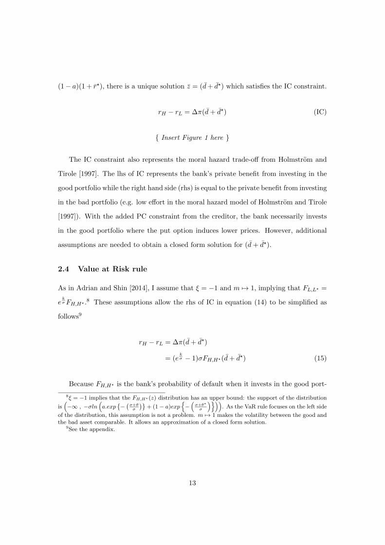
2.4 Value at Risk rule

As in Adrian and Shin [2014], I assume that ξ = −1 and m 7→ 1, implying that FL,L? =

ekσFH,H? .8 These assumptions allow the rhs of IC in equation (14) to be simplified as

follows9

rH − rL = ∆π(d+ d?)

= (ekσ − 1)σFH,H?(d+ d?) (15)

Because FH,H? is the bank’s probability of default when it invests in the good port-

8ξ = −1 implies that the FH,H?(z) distribution has an upper bound: the support of the distribution

is(−∞ , −σln

(a.exp

−(σ+θσ

)+ (1− a)exp

−(σ+θ?

σ

))). As the VaR rule focuses on the left side

of the distribution, this assumption is not a problem. m 7→ 1 makes the volatility between the good andthe bad asset comparable. It allows an approximation of a closed form solution.

9See the appendix.

13

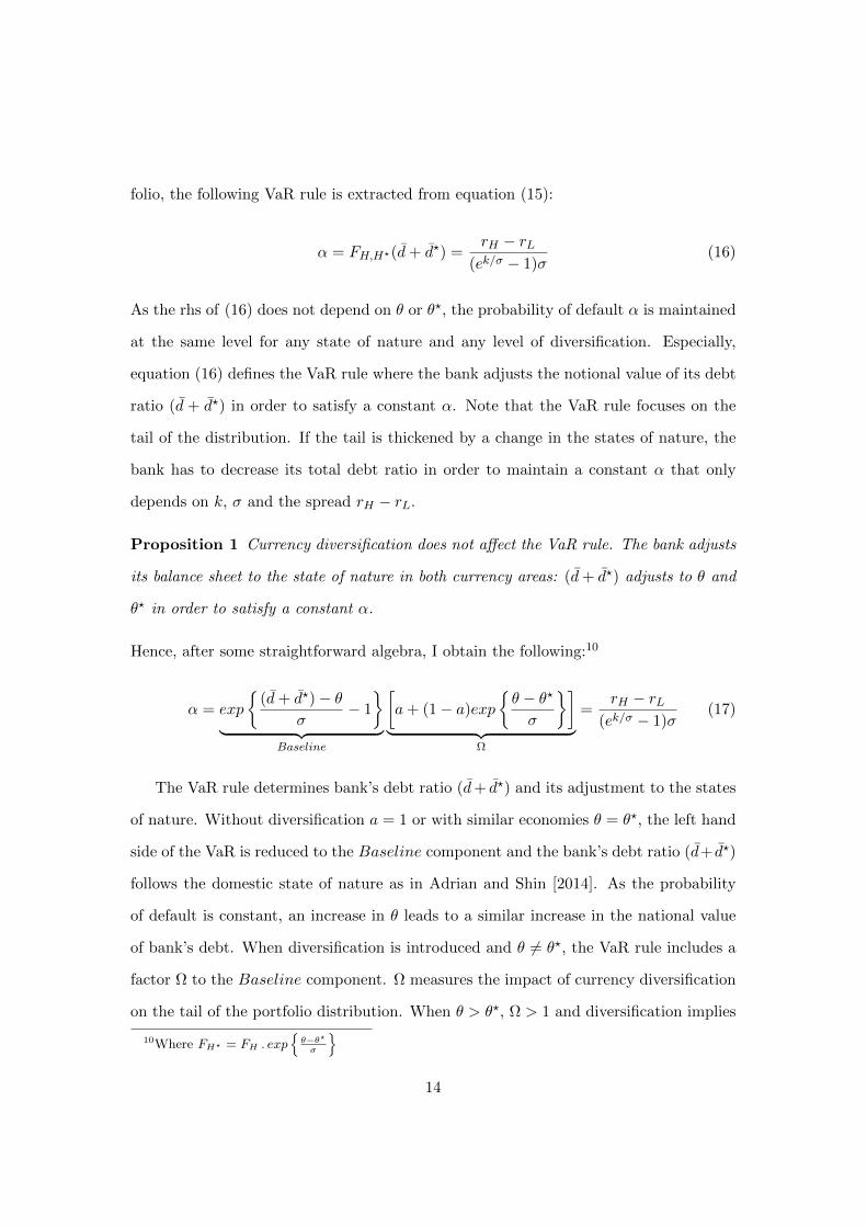
folio, the following VaR rule is extracted from equation (15):

α = FH,H?(d+ d?) =rH − rL

(ek/σ − 1)σ(16)

As the rhs of (16) does not depend on θ or θ?, the probability of default α is maintained

at the same level for any state of nature and any level of diversification. Especially,

equation (16) defines the VaR rule where the bank adjusts the notional value of its debt

ratio (d + d?) in order to satisfy a constant α. Note that the VaR rule focuses on the

tail of the distribution. If the tail is thickened by a change in the states of nature, the

bank has to decrease its total debt ratio in order to maintain a constant α that only

depends on k, σ and the spread rH − rL.

Proposition 1 Currency diversification does not affect the VaR rule. The bank adjusts

its balance sheet to the state of nature in both currency areas: (d+ d?) adjusts to θ and

θ? in order to satisfy a constant α.

Hence, after some straightforward algebra, I obtain the following:10

α = exp

(d+ d?)− θ

σ− 1

︸ ︷︷ ︸

Baseline

[a+ (1− a)exp

θ − θ?

σ

]︸ ︷︷ ︸

Ω

=rH − rL

(ek/σ − 1)σ(17)

The VaR rule determines bank’s debt ratio (d+ d?) and its adjustment to the states

of nature. Without diversification a = 1 or with similar economies θ = θ?, the left hand

side of the VaR is reduced to the Baseline component and the bank’s debt ratio (d+ d?)

follows the domestic state of nature as in Adrian and Shin [2014]. As the probability

of default is constant, an increase in θ leads to a similar increase in the national value

of bank’s debt. When diversification is introduced and θ 6= θ?, the VaR rule includes a

factor Ω to the Baseline component. Ω measures the impact of currency diversification

on the tail of the portfolio distribution. When θ > θ?, Ω > 1 and diversification implies

10Where FH? = FH . expθ−θ?σ

14

a thickening of the tail of the portfolio distribution: the diversified portfolio becomes

riskier than the baseline portfolio. In return, when θ < θ?, Ω < 1 and the tail of the

portfolio distribution becomes thinner than the tail of the portfolio distribution at the

baseline, implying a safer portfolio than the baseline portfolio.

Proposition 2 Under a fixed exchange rate, currency diversification increases the tail

risk of banks (Ω > 1) when the domestic economic condition outperforms the foreign

one (θ > θ?), while it decreases it (Ω < 1) when the foreign economic condition becomes

better than the domestic one (θ < θ?).

The VaR rule (17) then defines the adjustment of the bank’s debt ratio at the notional

value (d+ d?) to the states of nature θ, θ?, such that:

(d+ d?) = θ + σ + σln

(rH − rL

(ek/σ − 1)σ

)︸ ︷︷ ︸

Baseline

−σln

a+ (1− a)exp

θ − θ?

σ

︸ ︷︷ ︸

Ω

(18)

When θ = θ?, Ω = 1 implying an unchanged tail risk: during booms the baseline (d+ d?)

increases while it decreases during burst. It defines the baseline leverage procyclicality.

When θ > θ?, Ω > 1 and the tail risk increases: the increase in bank’s debt ratio at

the notional value is then less pronounced during booms than the baseline framework

would predict. (d+ d?) is less procyclical than the baseline. Similarly during burst, the

decrease in (d+ d?) is then less pronounced than the baseline framework would predict:

procyclicality increases. When θ? > θ, Ω < 1 and the tail risk decreases: during booms,

currency diversification increases the procyclicality of (d+ d?), but it decreases it during

burst.

Proposition 3 Valuation effect aside, leverage is more procyclical with currency diver-

sification than without when the foreign economic condition is more volatile than the

domestic one. When the foreign state of nature becomes less volatile than the domestic

one, leverage procyclicality then decreases.

15

Following equation (9), the debt ratio (d + d?) is a positive function of (d + d?),

implying that previous conclusions on (d + d?) are applied to leverage procyclicality

given that:

λ =1

1− (d+ d?)(19)

When the foreign economy outperforms the domestic economy, leverage procyclicality

is increased by currency diversification during booms but decreased by it during bursts.

When the domestic economy outperforms the foreign economy, leverage procyclicality

is then decreased by currency diversification during booms but increased by currency

diversification during bursts. Valuation effect aside, leverage is then more procyclical

with currency diversification than without when the foreign economic condition is more

volatile than the domestic one, that is when it outperforms the domestic economic condi-

tion during booms but falls behind it during bursts. Conversely, leverage procyclicality

decreases when the foreign state of nature is less volatile than the domestic one. Those

generalized conclusions support previous results from Kwok and Reeb [2000] which visit

the upstream downstream hypothesis of internationalization.

2.5 Introducing a floating exchange rate

In previous sections, the foreign exchange rate is assumed to be fixed. Floating ex-

change rate regime affects the weight of assets in the bank’s portfolio since a = AA+SA? .

Depending on the correlation between the exchange rate and asset returns, a floating

exchange rate will impact the portfolio distribution and the leverage adjustments.

The extensive empirical literature on the relationship between foreign exchange rates

and the state of nature of the economy or between foreign exchange rates and interest

rates suggests that domestic macroeconomic performances or relative domestic return

16

performances are associated with domestic currency appreciation. 11

Hypothesis 1 The domestic currency appreciates when the domestic return rises with

respect to the foreign one.

As θ and θ? are known for both periods T=0, 1, the exchange rate S does not

change between T=0 and T=1. The process of S relative to good portfolios is given by

equation (20) where returns depend on the state of nature of both economies and on a

function of the shape parameter H(ξ):

S = 1 +rH? − rH1 + rH

(20)

Where :

rH? =θ? + σH(ξ)

rH =θ + σH(ξ)

limrH→∞

S(rH) =0 , and S = 1 ↔ rH = rH?

As θ and θ? are known for both periods, the exchange rate does not change between

T=0 and T=1. Implicitly, I also assume that the bank does not change the composition

of its portfolio, notwithstanding small changes in states of nature.12 When the domestic

11Using high frequency data and macroeconomic announcements in the U.S or in Germany in the1990s, Andersen et al. [2003, 2007], Faust et al. [2007] show that the foreign exchange rate is linkedto macroeconomic fundamentals: a stronger than expected release appreciates the domestic currency.Regarding interest rates, Engel [1996] shows that the currency with the higher interest rate typicallyappreciates. Using structural VAR with daily data from 1988 to 2004, Ehrmann et al. [2011] show thatthe euro is also positively affected by shocks on short rates where a rise in euro area short rates leadsto a euro appreciation. Finally, Itskhoki and Mukhin [2017] define a theoretical model reproducing thedifferent foreign exchange rate puzzles identified in the literature, including the Engel [1996] result.

12This implicit assumption seems to be reasonable regardless of the time horizon because of boththe transaction costs and the international dimension of the foreign currency. Odean [1998], Liu andStrong [2008] justify the ”buy and hold” strategy for short term horizon because of the transaction costsimplied in rebalancing strategies. Following Liu and Strong [2008], a monthly rebalancing strategy isthen unrealistic. In addition, the foreign currency included in the model is considered as an internationalcurrency. Because of the international involvement of global banks, there is an incompressible share ofassets and liabilities denominated in foreign currency. A complete re-allocation from one currency toanother would then imply a complete change in the bank’s business model, going from global to nationaland vice-versa, or a complete change in the definition of the international monetary system. It seemsreasonable to think that such adjustments are rare and sluggish.

17

currency appreciates, the converted value of the foreign asset declines, which leads to a

larger share of domestic assets relative to total assets: a goes up at T=0, 1. Conse-

quently, the changes in a and (1− a) only reflect the exchange rate effect on converted

value, so called the valuation effect of currency diversification. This makes it possible

to identify the impact of currency diversification on leverage.

Hypothesis 2 Changes in a only reflect valuation effects due to variations in the ex-

change rate, that is da(S)dS < 0.

One can rewrite equation (18) where a is a function of S such that:

(d+ d?) = θ + σ + σln

(rH − rL

(ek/σ − 1)σ

)− σln

a(S) + (1− a(S)) exp

θ − θ?

σ

︸ ︷︷ ︸

ΩS

(21)

Withda(S)

dS< 0

Because a floating exchange rate always promotes the asset which offers a better return

in the portfolio, S directly affects the tail of the portfolio distribution through ΩS .

Compared to a fixed exchange rate regime, the introduction of S as defined in equation

(20) always decreases the thickness of the distribution tail. As the bank still follows

the VaR rule, the floating exchange rate regime increases its capacity to raise funds

compared to its debt capacity in a fixed exchange rate regime.

Proposition 4 Introducing a floating exchange rate, the valuation effect decreases the

tail risk of banks and increases their fund-raising capacity as long as the two economies

are different, that is d(d+d?)dS > 0 when θ? > θ or d(d+d?)

dS < 0 when θ? < θ.

The valuation effect, or the effect of a floating exchange rate regime on (d+d?) compared

to the fixed exchange rate regime is observed through the derivative of (d+ d?) relative

18

to S when θ and θ? are constant:

d(d+ d?)

dS| θ, θ? = −σ

(da(S,θ,θ?)

dS | θ, θ?) (

1− expθ−θ?σ

)a+ (1− a)exp

θ−θ?σ

(22)

When the exchange rate regime is floating, S does not affect (d+ d?) when θ = θ?.

An appreciation of the foreign currency (i.e S increases) leads to an increase in (d+ d?)

when:

(da(S,θ,θ?)

dS| θ, θ?

)(1− exp

θ − θ?

σ

)< 0 (23)

Because(da(S,θ,θ?)

dS | θ, θ?)< 0, then the condition becomes θ? > θ. Foreign currency

appreciates when the the foreign economy outperforms the domestic one, leading to

an increase in the fund raising capacity. Alternatively, an appreciation of the domes-

tic currency (i.e S decreases) leads to an increase in (d + d?) when θ > θ? because(da(S,θ,θ?)

dS | θ, θ?)< 0. Domestic currency appreciates when the domestic economy out-

performs the foreign one and leads to an increase in the bank’s fund raising capacity. The

conditions allowing an increase in fund raising capacities depend on the definitions of

the model. The difference in the states of nature defines the exchange rate adjustment

while(da(S,θ,θ?)

dS | θ, θ?)< 0 defines the portfolio adjustment relative to the exchange

rate. In this framework, a floating exchange rate regime always increases the bank’s

fund raising capacity compared to a fixed exchange rate regime when θ 6= θ?.

Combining both the diversification and the valuation effects introduces conditions

for leverage counter-cyclicality. When the domestic economy outperforms the foreign

one during a burst, θ > θ?, leverage procyclicality is increased by the diversification

effect but decreased by the valuation effect due to the floating exchange rate. Similarly,

when the foreign economy outperforms the domestic one during a burst, θ? > θ, leverage

procyclicality is decreased by both the diversification effect and the valuation effect. If

19

the valuation effect is strong enough during economic bursts, leverage may then become

counter-cyclical if the initial currency diversification satisfies a given threshold.13 When

θ > θ?, the condition for a counter-cyclical leverage relative to the foreign economic

condition is such that:

(1− a)

(da(S,θ,θ?)

dθ?| θ)−1

︸ ︷︷ ︸Portfolio adjustment

< σ

(1

expθ−θ?σ

− 1

)︸ ︷︷ ︸

∆Economic condition

(24)

The counter-cyclical condition in equation (24) compares the portfolio adjustment due

to the valuation effect to the relative economic performance going from θ = θ? to θ > θ?

with θ being constant. As(da(S,θ,θ?)

dθ? | θ)< 0, the higher the initial share of foreign

asset, the more the bank benefits from the valuation effect and the more validated the

condition would be. Because the foreign economy is bursting, the domestic currency

appreciates and the valuation effect promotes the domestic asset in bank’s portfolio:

the valuation effect decreases the tail risk and offsets the economic burst.

When the domestic economy contracts (θ < θ?), a counter-cyclical leverage relative

to the domestic economic condition is observed when the valuation effect is larger than

the decline in economic condition. With(da(S,θ,θ?)

dθ | θ?)> 0, the condition becomes:

a

(da(S,θ,θ?)

dθ| θ?)−1

︸ ︷︷ ︸Portfolio adjustment

< σ

(1− exp

θ − θ?

σ

)︸ ︷︷ ︸

∆Economic condition

(25)

The lower the initial share of domestic asset in the bank’s portfolio, the more beneficial

the valuation effect is and the more validated the condition would be.

Table 2 summarizes the theoretical predictions from the model. The impact of cur-

13See the appendix for more details.

20

rency diversification on leverage procyclicality then depends on the relative performance

of the two economies, the business cycle, and the exchange rate regime.

Table 2: Impact of currency diversification on leverage procyclicality. Thecomparative is the baseline leverage procyclicality (i.e without diversification), or theleverage procyclicality under the fixed exchange rate regime for the impact of floatingexchange rate regime.

Generalized conclusions with fixed FX and positive correlation between θ and θ?:

σθ? < σθ: Less procyclicalσθ? > σθ: More procyclicalσθ? = σθ: Unchanged

During booms: During bursts:

Similar economies: θ? = θFixed FX Unchanged Unchanged→ Introducing floating FX Unchanged Unchanged

Foreign economy outperforms: θ? > θ

Fixed FX More procyclical Less procyclical→ Introducing floating FX Procyclicality Procyclicality

(Potentially counter-cyclical)

Domestic economy outperforms: θ > θ?

Fixed FX Less procyclical More procyclical→ Introducing floating FX Procyclicality Procyclicality

(Potentially counter-cyclical)

2.6 Discussion

Following theoretical conclusions, the only driving force of leverage fluctuations is the

portfolio distribution which depends on both states of nature and the foreign exchange

rate: the composition of bank’s debt is not determinant to the definition of leverage

procyclicality. In other terms, currency mismatch does not affect leverage procyclical-

ity. There is a threefold explanation for this phenomenon.

21

First, the contracting problem introduces a participation constraint and an incentive

constraint that micro-found the VaR rule. The only source of adjustment of banking

leverage comes from the asset side: total converted debt adjusts to changes in total

converted asset. In this framework, introducing an exogenous debt interest rate would

change the definition of the two constraints that defined the VaR rule. Similarly, a risk-

free interest rate removes the contracting model and fails to micro-found the VaR rule.

Considering a potential monetary policy interest rate, the framework defined in this

paper is still compatible as long as the interest rate defined by the contracting model

stays above the monetary policy interest rate.14

Second, the bank supports foreign exchange rate fluctuations only through its total

portfolio returns. The impact of foreign exchange rate fluctuations on bank’s debt is

supported by the creditor of the bank. Assuming that the bank only invests in domestic

asset while it raises debt in foreign currency. An improvement of the foreign economic

condition does not change the portfolio return distribution as it only contains domestic

asset. According to the VaR rule, the bank’s leverage is unchanged, implying similar

total converted debt and reimbursement. Implicitly, it means that the appreciation of

the foreign currency is internalized by the bank’s creditor. The total converted debt

and reimbursement stay unchanged, but the total debt and reimbursement in foreign

currency decrease.

Third, as the states of nature are known for the two periods, S is fixed for T = 0, 1,

removing the traditional risk implied by currency mismatch. For each state of nature,

a new contract is defined where the foreign exchange rate is known.

14In Bruno and Shin [2015], Coimbra and Rey [2017], the VaR rule is directly implemented to constrainbanks’ leverage. The interest rate on deposits is then riskfree or exogenous, introducing a second sourceof adjustment for banking leverage on the liability side: the monetary policy. However, this frameworkdoes not enable the microfoundations of the VaR rule as in Adrian and Shin [2014].

22

3 Quantitative analysis

Focusing on the 2008-2009 crisis, the theoretical model predicts that banks with expo-

sures to the US and the US dollar are supposed to show different leverage procyclicality.

Considering banks in France and the major economic and financial negative shock com-

ing from the US during the 2008-2009 crisis, currency diversification is expected to

increase leverage procyclicality during this period. Focusing on the valuation effect of

currency diversification, however; one can expect that it has a negative impact on lever-

age procyclicality. This section is devoted to the quantitative analysis of the theoretical

predictions using micro-data on banks located in France during the 2008-2009 crisis.

3.1 Data

I use a unique micro-data from the French banking supervision authority ACPR. It con-

sists of foreign and French banks located in France and it provides yearly information

on consolidated banks’ balance sheet and derivatives relative to foreign exchange rate

operations, and on a proxy of the currency diversification of assets.15 Additionally, it

provides information on banks’ characteristics such as the nationality of banks and the

sub-category the banks are attached to (banks, cooperative banks, financial and invest-

ment firms).

Focusing on the 2008-2009 crisis, the sample consists of 26 banks composed of 18

and 8 French and foreign banks, respectively. Table 3 provides descriptive statistics

on all banks focusing on banks’ size defined as the logarithm of total assets, leverage

defined as the ratio of total assets to equity, US dollar diversification defined as the

share of assets denominated in US dollar FX2007, US dollar diversification with euro

area counterparties FX(EA)2007 and derivatives relative to foreign exchange operations

defined as the ratio of those derivatives to total assets Deriv2007. The general decrease

15See the appendix for more details on data

23

in leverage and total assets between 2008 and 2009 is confirmed, where leverage and

total assets decreased by 15% and 8% on average, respectively.

Insert Table 3 here

Following table 3, banks had an average US dollar diversification of 12% of total

assets in 2007, while the FX derivative ratio reached 0.54 on average for the same year.

Focusing on standard deviations, minimum and maximums, heterogeneity is observed in

all variables reported in table 3. Tables 4 and 5 provide additional descriptive statistics

focusing on French or foreign banks. Comparing the two tables, foreign banks are more

diversified in 2007 than French banks. They also manifest stronger decline in leverage

and size during the financial crisis than their French counterparts.

Insert Table 4 5 here

3.2 Empirical model

I focus on the impact of currency diversification on leverage procyclicality during the

2008-2009 crisis. Especially, I want to test whether the pre-crisis currency diversification

of assets, i.e in 2007, affects the large adjustment of banks’ balance sheet during the

crisis, i.e between 2008 and 2009. My quantitative analysis is thus based on cross-section

heterogeneity between banks.

I follow previous empirical strategies used in Adrian and Shin [2008], Kalemli-Ozcan

et al. [2012], Baglioni et al. [2013], Damar et al. [2013] where the growth rate of leverage

between 2008 and 2009 is the dependent variable and the value of leverage in 2008 and

the growth rate of assets between 2008 and 2009 are the main explanatory variables.16

Leverage procyclicality is then measured with the coefficient β2 in equation (26). I ex-

tend the specification by introducing an interaction term between the growth rate of

16∆ stands for the first-difference of the logarithm.

24

assets between 2008 and 2009 and the level of currency diversification in 2007 FXi,2007.

The coefficient β3 then measures the effect of currency diversification on leverage pro-

cycliclality.17 I add the level of currency diversification and the FX derivative ratio in

2007 Derivi,2007 as control variables. Finally, to control for unobserved heterogeneity

between banks I introduce several dummy variables δi including a French national-

ity dummy variable and dummy variables capturing the category of banks. Banking

categories cover general banks, cooperative banks, specialized banks (i.e ECS) and spe-

cialized financial institutions (i.e IFS). ECS are specialized in specific financial activities

including consumer loans and mortgage financial leases, while IFS are credit institu-

tions with a specific mandate defined by public authorities. I believe that these dummy

variables for banks’ category and nationality may then avoid issues related to omitted

factors that potentially co-determine both the choice of currency diversification prior

the financial crisis as well as the movement of leverage afterward.18

∆Leveragei,2008−09 = α+ β1 ln(Leveragei,2008) + β2 ∆Asseti,2008−09

+ β3 (∆Asseti,2008−09 x FXi,2007) + β4 FXi,2007

+ β5 Derivi,2007 +

10∑j=6

βjδj,i + ui (26)

The variable FX2007 captures both the diversification and the valuation effects. In

order to capture the valuation effect of currency diversification I extend the analysis by

17I believe that the risk of reverse causality between the crisis leverage adjustment and the pre-crisiscurrency diversification is limited because of the unexpected nature of the financial crisis. The ideaof reverse causality implies that the choice of currency diversification is determined by future leverageadjustment (or targeted leverage adjustment). Applying this hypothesis to the financial crisis, it wouldmean that banks have chosen their pre-crisis currency diversification in order to achieve their crisisleverage adjustment. As financial crisis are by definition unexpected, then the risk of reverse causalityseems to be reduced.

18Because of their specific activities, then ECS and IFS are not expected to show either large currencydiversification or large leverage procyclicality compared to general banks. Similarly, foreign banks lo-cated in France are expected to have more currency diversification than French banks; but they are alsoexpected to be more procyclical than French banks as they are the first adjustment variable for foreignglobal banks during financial crisis.

25

replacing the share of assets denominated in US dollar by the share of assets denomi-

nated in US dollar with euro area counterparties FX(EA).19 Considering the euro area

counterparty as a resident counterparty, this new measure of currency diversification

only captures the valuation effect of diversification. An alternative to test the robust-

ness of my results might be to replace the currency diversification measure by the FX

derivative measure as it focuses on derivatives relative to foreign exchange operations

only. This last specification implies to introduce the currency diversification measure as

a control variable.

3.3 Quantitative results

Table 6 reports results from the different specifications of (26). For all specifications,

results confirm previous conclusions from the literature: leverage is a mean reverting

process and it is procyclical. However, my results also show that leverage prcyclicality

depends on currency diversification.

Insert Table 6 here

Focusing on currency diversification with all conterparties FX2007, the results show

that currency diversification had increased leverage procyclicality during the crisis. This

first conclusion is robust even when the pre-crisis currency diversification is defined in

2006 instead of 2007. However, the measure of currency diversification FX captures

the two effects of currency diversification. Because of the floating exchange rate regime,

the theoretical model predicts a decrease in leverage procyclicality due to the valuation

effect. Therefore, results reported in column (1) and (3) suggest that the diversification

effect dominates the valuation effect. To capture the valuation effect, I introduce the

variable FX(EA) in column (2) and (5). The results confirm this prediction where

19The share of assets denominated in euro with US counterparties or with non-euro area counterpartiesmay capture the pure diversification effect. However, that information is not available in the currentdatabase.

26

currency diversification relative to euro area FX(EA) captures this valuation effect:

valuation effect reduces leverage pro-cyclicality. Using the ratio of the FX derivative

Deriv as an alternative measure of the valuation effect supports my conclusions at least

when the measure is taken in 2007. Comparing the different results between column

(1) and (2), my results suggest that the diversification effect, apart from the valuation

effect, increases leverage procyclicality. They also support the implicit assumption that

banks do not change their portfolio allocation at each period.20

Figure 2 illustrates the previous results and reports the predicted leverage procycli-

cality for different levels of 2007 pre-crisis currency diversification. The total currency

diversification effect increases leverage procyclicality when currency diversification goes

from 0 to the average value (i.e 0.12). When the maximum pre-crisis currency diversifi-

cation is assumed (i.e 0.71), the slope of the line is even more stronger than previously,

translating the large sensitivity to foreign economic choc.

Insert Figure 2 here

Focusing on the valuation effect, we observed that the predicted leverage pro-cyclicality

is lower for average value of pre-crisis currency diversification (i.e. 0.03) than for 0

currency diversification, even if this average pre-crisis currency diversification is quite

low. Interestingly, our results also supports the theoretical prediction which suggests a

counter-cyclical leverage due to the valuation effect and a significant pre-crisis currency

diversification.

20If banks re-allocate their portfolio at each period, then the number of lags used for currency diver-sification would be determinant to capture the effect of pre-crisis currency diversification on leverageprocyclicality during the crisis.

27

4 Conclusion

By introducing currency diversification in both sides of bank’s balance sheet, this paper

provides an adjusted framework to European banks with two currency denominations

for assets and debts, corresponding to two different countries. It implies a diversifica-

tion of risks between the two countries and a valuation effect from floating exchange rate.

The international dimension of banking activities associated to the Value-at-Risk rule

offer a new framework to explain the heterogeneous procyclicality of leverage where the

currency diversification of balance sheet plays a key role. When the foreign economy

outperforms the domestic one, a currency diversification reduces risk in bank’s port-

folio. Currency diversification then increases leverage procyclicality during booms but

decreases it during bursts as it expands the bank’s capacity to raise funds. Inversely, risk

in bank’s portfolio gets larger with currency diversification when the domestic economy

outperforms the foreign one: currency diversification decreases leverage procyclicality

during booms but increases it during bursts. More broadly, currency diversification

increases leverage procyclicality when it implies a foreign economic condition that is

more volatile than the domestic economic condition. Introducing a floating exchange

rate then expands the bank’s capacity to raise funds, since currency appreciates when

its associated economy outperforms others. The bank’s leverage procyclicality then de-

pends on the relative performance of countries, the business cycle, the level of currency

diversification and the exchange rate regime.

As this framework introduces currency diversification heterogeneity as an additional

variable to explain the heterogeneous cyclical variations of leverage, it allows me to

make use of cross-sectional data on banks’ balance sheet. Focusing on banks located

in France during the 2008-2009 crisis, my results show that leverage procyclicality pos-

itively depends on bank’s pre-crisis currency diversification. The higher the currency

28

diversification before the crisis, the stronger the leverage response to assets variations

during the 2008-2009 crisis. Focusing on the valuation effect of currency diversification,

my results show that it reduces leverage procyclicality during the crisis. Therefore, the

empirical results yield supporting evidence to the theoretical predictions where the do-

mestic economy outperforms the foreign economy during a burst.

This paper underlines the specific role of balance sheet currency diversification in

financial stability risk and economic stability. As not all foreign currencies and foreign

economies are alike, this paper shows that the impact of currency diversification would

differ according to which currency denomination is included. Therefore, policy recom-

mendations on international banking activities need to be identified in respect to the

characteristics of foreign exchange rates and the relative economic and financial perfor-

mances.

This paper offers a large range of potential extensions. First, a major advantage

of this model is its flexibility, especially regarding the definition of exchange rate and

the portfolio rebalancing behavior. Changing the bank’s strategy from a ”buy and

hold” strategy to an active rebalancing strategy can be described simply by changing

the assumption on the portfolio adjustments to economic conditions. Then, this paper

suggests that the amplification of economic booms and bursts due to leverage cyclical

variations depends to the extent of international banking activities. Applying this model

to a general equilibrium model may then provide an interesting framework for future

research. Finally, this paper raises the question of asymmetries between booms and

burst, especially if the volatility of the economic conditions is time varying. Extending

the quantitative analysis to both a panel data analysis and a broader currency portfolio

is a subject of keen interest than I plan to cover in future research.

29

References

T. Adrian and H. S. Shin. Liquidity and financial cycles. BIS WP 256, 2008.

T. Adrian and H. S. Shin. Procyclical leverage and Value-at-Risk. Review of Financial

Studies, 27:373–403, 2014.

T. Andersen, T. Bollerslev, F. Diebold, and C. Vega. Micro effects of macro announce-

ments: Real-time price discovery in foreign exchange. American Economic Review,

93:38–62, 2003.

T. Andersen, T. Bollerslev, F. Diebold, and C. Vega. Real-time price discovery in global

stock, bond and foreign exchange markets. Journal of International Economics, 73:

251–277, 2007.

N. Baba, R. McCauley, and S. Ramaswamy. US dollar money market funds and non-us

banks. BIS Quarterly Review, 2009.

A. Baglioni, E. Beccalli, A. Boitani, and A. Monticini. Is the leverage of european banks

procyclical? Empirical Economics, 45:1251–1266, 2013.

Y. Baskaya, J. di Giovanni, S. Kalemli-Ozcan, and M. Ulu. International spillovers and

local credit cycles. NBER Working Paper No. 23149, 2017.

S. Benoit, G. Colletaz, C. Hurlin, and C. Perignon. A theoretical and empirical com-

parison of systemic risk measures. HEC Paris Research Paper No. FIN-2014-1030,

2013.

V. Bruno and H. S. Shin. Cross-border banking and global liquidity. Review of Economic

Studies, 82:535–564, 2015.

E. Cerutti, S. Claessens, and L. Ratnovski. Global liquidity and cross-border bank flows.

Economic Policy, 32:81–125, 2017.

N. Coimbra and H. Rey. Financial cycles with heterogeneous intermediaries. NBER

Working Paper, 23245, 2017.

E. Damar, C. Meh, and Y. Terajima. Leverage, balance-sheet and wholesale funding.

Journal of Financial Intermediation, 22:639–662, 2013.

J. Danielsson., H. S. Shin, and J.-P. Zigrand. Procyclical leverage and endogenous risk.

Princeton University, 2012.

30

M. Ehrmann, M. Fratzscher, and R. Rigobon. Stocks, bonds, money markets and

exchange rates: measuring international financial transmission. Journal of Applied

Econometrics, 26:948–974, 2011.

C. Engel. The forward discount anomaly and the risk premium: A survey of recent

evidence. Journal of Empirical Finance, 3:123–191, 1996.

J. Faust, J. Rogers, SY. Wang, and J. Wright. The high-frequency response of exchange

rates and interest rates to macroeconomic announcements. Journal of Monetary Eco-

nomics, 54:1051–1068, 2007.

H. Hau and H. Rey. Global portfolio rebalancing under the microscope. NBER Working

Paper, 14165, 2008.

B. Holmstrom and J. Tirole. Financial intermediation, loanable funds, and the real

sector. Quarterly Journal of Economics, 112:663–691, 1997.

O. Itskhoki and D. Mukhin. Exchange rate disconnect in general equilibrium. NBER

Working Paper, 23401, 2017.

S. Kalemli-Ozcan, B. Sorensen, and S. Yesiltas. Leverage across firms, banks and coun-

tries: some evidence from banks. Journal of International Economics, 88:284–298,

2012.

S. Krogstrup and C. Tille. On the roles of different foreign currencies in european bank

lending. SNS Working Paper, 2016.

S. Krogstrup and C. Tille. Foreign currency bank funding and global factors. Manuscript,

Graduate Institute and International Monetary Fund, 2017.

C. Kwok and D. Reeb. Internationalization and firm risk: an upstream-downstrean

hypothesis. Journal of International Business Studies, 31:611–629, 2000.

W. Liu and N. Strong. Biases in decomposing holding-period portfolio returns. The

Review of Financial Studies, 21:2243–2274, 2008.

R. Merton. On the pricing of corporate debt: the risk structure of interest rates. Journal

of Finance, 29:449–470, 1974.

G-M. Milesi-Ferretti, C. Tille, G. Ottaviano, and M. Ravn. The great retrenchment:

international capital flows during the global financial crisis. Economic Policy, 26:

289–346, 2011.

31

T. Odean. Are investors reluctant to realize their losses? The Journal of Finance, 53:

1775–1798, 1998.

R. Reiss and M. Thomas. Statiscal analysis of extreme values. Birkhuser Basel, 3rd

edition, 2007.

H. S. Shin. Global banking glut and loan risk premium. IMF Economic Review, 60:

155–192, 2012.

32

Appendix

A The model

A.1 Constant spreads

As assets only differ in their location parameters, the spread between the good and the

bad investment returns is equal for domestic as for foreign currency assets:

rH − rL = θ + σH(ξ)− (θ − k)−mσH(ξ)

= k − σ(m− 1)H(ξ)

And :

rH? − rL? = θ? + σH(ξ)− (θ? − k)−mσH(ξ)

= k − σ(m− 1)H(ξ)

Therefore:

a(rH − rL) + (1− a)(rH? − rL?)

= a. (θ + σH(ξ)− (θ − k)−mσH(ξ)) + (1− a) (θ? + σH(ξ)− (θ? − k)−mσH(ξ))

= a. (k − σ(m− 1)H(ξ)) + (1− a) (k − σ(m− 1)H(ξ))

= (k − σ(m− 1)H(ξ))

= Cst

A.2 IC development

The simplifying assumptions give the following IC constraint:

(rH − rL) = ∆π(d+ d?) (A.1)

=

∫ d+d?

0FL,L? dz −

∫ d+d?

0FH,H? dz

= ekσ

∫ d+d?

0FH,H? dz −

∫ d+d?

0FH,H? dz

= (ekσ − 1)

∫ d+d?

0FH,H? dz

= (ekσ − 1)σFH,H?(d+ d?)

33

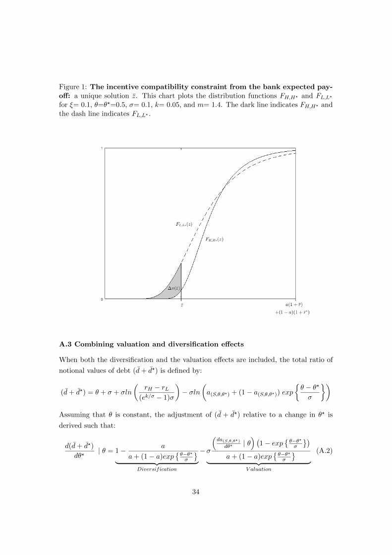
Figure 1: The incentive compatibility constraint from the bank expected pay-off: a unique solution z. This chart plots the distribution functions FH,H? and FL,L?

for ξ= 0.1, θ=θ?=0.5, σ= 0.1, k= 0.05, and m= 1.4. The dark line indicates FH,H? andthe dash line indicates FL,L? .

A.3 Combining valuation and diversification effects

When both the diversification and the valuation effects are included, the total ratio of

notional values of debt (d+ d?) is defined by:

(d+ d?) = θ + σ + σln

(rH − rL

(ek/σ − 1)σ

)− σln

(a(S,θ,θ?) + (1− a(S,θ,θ?)) exp

θ − θ?

σ

)Assuming that θ is constant, the adjustment of (d + d?) relative to a change in θ? is

derived such that:

d(d+ d?)

dθ?| θ = 1− a

a+ (1− a)expθ−θ?σ

︸ ︷︷ ︸Diversification

−σ

(da(S,θ,θ?)

dθ? | θ) (

1− expθ−θ?σ

)a+ (1− a)exp

θ−θ?σ

︸ ︷︷ ︸V aluation

(A.2)

34

Where the derivative is composed of two effects, the diversification effect and the valu-

ation effect. When the exchange rate is fixed (i.eda(S,θ,θ?)

dθ? = 0), the derivative is limited

to the diversification effect. It is equal to 0, 1 and (1−a) when a = 1, a = 0 and θ = θ?,

respectively. When the states of nature become different θ 6= θ? with θ being fixed, a

currency diversification implying that a > 0 reduces the procyclicality of (d+d?) relative

to the foreign state of nature: the stability of the domestic state of nature anchors the

tail risk of asset portfolio.

A floating exchange rate introduces a valuation effect as long as θ 6= θ?. Its impact

on the adjustment of (d + d?) relative to a change in θ? depends on the adjustments

of the foreign state of nature. When the foreign economy is booming (θ? > θ), the

valuation effect is positive and increases the procyclicality of (d + d?) relative to θ?.

The foreign economic condition implies a depreciation of the domestic currency and

a decrease in the share of the domestic asset in the bank’s portfolio: the tail risk is

reduced. Similarly, when the foreign economy is bursting, θ? < θ, the valuation effect is

negative and reduces the procyclicality of (d+ d?) relative to the foreign state of nature.

The floating exchange rate promotes the domestic asset which performs relatively better

than the foreign one because of domestic currency appreciation. In both cases, a floating

exchange rate increases the fund raising capacity of banks. However, the adjustment

of (d + d?) relative to θ? may become counter-cyclical if the valuation effect is large

enough to compensate the diversification effect when the foreign economy is bursting.

A counter-cyclical (d+ d?) is observed when θ? < θ and:

(1− a)

(da(S,θ,θ?)

dθ?| θ)−1

︸ ︷︷ ︸Portfolio adjustment

< σ

(1

expθ−θ?σ

− 1

)︸ ︷︷ ︸

∆Economic condition

(A.3)

The counter-cyclical condition in equation (A.3) compares the portfolio adjustment due

to the valuation effect to the relative economic growth starting from θ = θ?. Because(da(S,θ,θ?)

dθ? | θ)< 0, the higher the initial share of foreign asset, the more validated the

condition.

Inversely when θ? is constant, the adjustment of (d + d?) relative to a change in θ

35

can be derived such that:

d(d+ d?)

dθ| θ? =

a

a+ (1− a)expθ−θ?σ

︸ ︷︷ ︸Diversification

−σ

(da(S,θ,θ?)

dθ | θ?) (

1− expθ−θ?σ

)a+ (1− a)exp

θ−θ?σ

︸ ︷︷ ︸V aluation

(A.4)

The derivative is equal to 0, 1 and a if a = 0, a = 1 and θ = θ?, respectively. The

procyclicality of (d+ d?) relative to a change in θ decreases when θ 6= θ? with θ? and S

being fixed, a currency diversification implying that (1−a) > 0 reduces the procyclicality

of (d+ d?) relative to the domestic state of nature: the stability of the foreign state of

nature anchors the tail risk of asset portfolio. Similarly to equation (A.2), a floating

exchange rate with θ 6= θ? introduces a valuation effect which depends on economic

conditions. When θ > θ?, the domestic economy outperforms the foreign one and

the domestic currency appreciates, implying that(da(S,θ,θ?)

dθ | θ?)> 0. The share of

domestic asset in bank’s portfolio raises and the bank fund raising capacity increases:

the valuation effect increases the procyclicality of (d + d?) relative to θ. Inversely, the

foreign economy outperforms the domestic one when θ < θ?, leading to an increase of

the bank’s fund raising capacity and a decrease in the procyclicality of (d+ d?) relative

to θ. When the valuation effect is strong enough to compensate the domestic burst, the

adjustment of (d+ d?) relative to θ may become counter-cyclical if:

a

(da(S,θ,θ?)

dθ| θ?)−1

︸ ︷︷ ︸Portfolio adjustment

< σ

(1− exp

θ − θ?

σ

)︸ ︷︷ ︸

∆Economic condition

(A.5)

The lower the initial share of domestic asset in the bank’s portfolio, the more the bank

benefits from the valuation effect and the more validated the condition would be.

B Quantitative analysis

The final database I use is a combination different databases collected by the French

banking supervision authority (ACPR) including the following eSurfi tables: SITUATION,

BILA CONS, F 01.00, F 11.01, DEVI SITU. Accounting data total assets, leverage

and derivatives are collected at the book value for the highest level of consolidation.

For large international banks, data are consolidated using the IFRS accounting stan-

dard and collected in Finrep tables F 01.00, F 11.01. Smaller parent banks provide

consolidated data using the French accounting standards (FRGAAP) in BILA CONS,

36

while stand-alone banks provide unconsolidated data reported in the SITUATION ta-

ble. Data on currency exposures (from DEVI SITU) are collected at the book value and

at an individual level for all banks (unconsolidated data). The proxy of asset currency

diversification adds up currency exposures of all affiliates in the same banking group.

Currency diversification is then an aggregate measure of the currency exposure at the

banking group level.

Table 3 provides descriptive statistics on banks focusing on bank’s size defined as

the logarithm of total assets, leverage defined as the ratio of total assets to equity, US

dollar diversification FX defined as the share of total assets denominated in US dollar,

US dollar diversification with euro area counterparties FX(EA) defined as the share

of total assets denominated in US dollar and including a euro area counterparty and,

derivatives relative to foreign exchange operations defined as the ratio of those deriva-

tives to total assets.

Table 3: Summary statistics: all banks

Variable Mean Std. Dev. Min. Max. N

Leverage2008 14.82 11.79 1.16 50.88 26ln(Asset)2008 9 2.72 5.64 14.5 26∆ ln(Leverage)2008−2009 -0.15 0.24 -0.89 0.21 26∆ ln(Asset)2008−2009 -0.08 0.21 -0.47 0.42 26FX2007 0.12 0.18 0 0.71 26FX(EA)2007 0.03 0.04 0 0.14 26Deriv2007 0.54 1.26 0 5.74 26

∆ stands for the first difference of variable between t and t− 1.

Table 4: Summary statistics: French banks

Variable Mean Std. Dev. Min. Max. N

Leverage2008 13.91 10.23 1.16 37.01 18ln(Asset)2008 9.49 2.9 5.64 14.5 18∆ ln(Leverage)2008−2009 -0.11 0.19 -0.46 0.21 18∆ ln(Asset)2008−2009 -0.02 0.2 -0.47 0.42 18FX2007 0.05 0.07 0 0.27 18FX(EA)2007 0.03 0.04 0 0.14 18Deriv2007 0.73 1.47 0 5.74 18

∆ stands for the first difference of variable between t and t− 1.

37

Table 5: Summary statistics: foreign banks

Variable Mean Std. Dev. Min. Max. N

Leverage2008 16.89 15.34 5.66 50.88 8ln(Asset)2008 7.89 2.01 6.24 12.49 8∆ ln(Leverage)2008−2009 -0.25 0.33 -0.89 0.09 8∆ ln(Asset)2008−2009 -0.19 0.2 -0.47 0.04 8FX2007 0.28 0.25 0.02 0.71 8FX(EA)2007 0.05 0.04 0 0.11 8Deriv2007 0.1 0.2 0 0.55 8

∆ stands for the first difference of variable between t and t− 1.

Figure 2: Predicted leverage procyclicality and currency diversification: pre-crisis currency diversification is measured in 2007 based on our sample data detailed intable 3

(a) Total diversification: FX (b) Valuation effect:FX(EA)

38

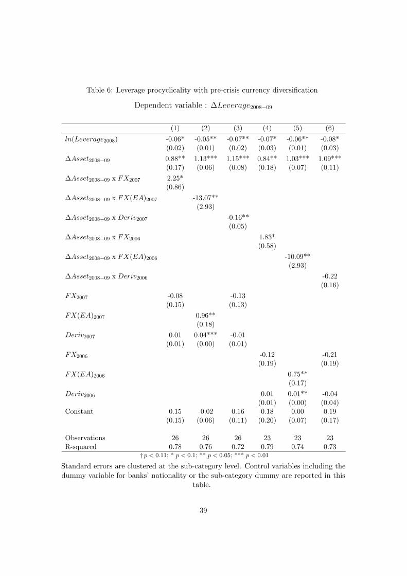
Table 6: Leverage procyclicality with pre-crisis currency diversification

Dependent variable : ∆Leverage2008−09

(1) (2) (3) (4) (5) (6)

ln(Leverage2008) -0.06* -0.05** -0.07** -0.07* -0.06** -0.08*(0.02) (0.01) (0.02) (0.03) (0.01) (0.03)

∆Asset2008−09 0.88** 1.13*** 1.15*** 0.84** 1.03*** 1.09***(0.17) (0.06) (0.08) (0.18) (0.07) (0.11)

∆Asset2008−09 x FX2007 2.25*(0.86)

∆Asset2008−09 x FX(EA)2007 -13.07**(2.93)

∆Asset2008−09 x Deriv2007 -0.16**(0.05)

∆Asset2008−09 x FX2006 1.83*(0.58)

∆Asset2008−09 x FX(EA)2006 -10.09**(2.93)

∆Asset2008−09 x Deriv2006 -0.22(0.16)

FX2007 -0.08 -0.13(0.15) (0.13)

FX(EA)2007 0.96**(0.18)

Deriv2007 0.01 0.04*** -0.01(0.01) (0.00) (0.01)

FX2006 -0.12 -0.21(0.19) (0.19)

FX(EA)2006 0.75**(0.17)

Deriv2006 0.01 0.01** -0.04(0.01) (0.00) (0.04)

Constant 0.15 -0.02 0.16 0.18 0.00 0.19(0.15) (0.06) (0.11) (0.20) (0.07) (0.17)

Observations 26 26 26 23 23 23R-squared 0.78 0.76 0.72 0.79 0.74 0.73

† p < 0.11; * p < 0.1; ** p < 0.05; *** p < 0.01

Standard errors are clustered at the sub-category level. Control variables including thedummy variable for banks’ nationality or the sub-category dummy are reported in this

table.

39