How do various maize crop models vary in their responses to climate change factors?

How do various maize crop models vary in theirresponses to climate change factors?S IMONA BASSU 1 , NAD INE BR I S SON 1 † , J EAN -LOU I S DURAND2 , KENNETH BOOTE 3 ,

JON L IZASO 4 , JAMES W . JONES 5 , CYNTH IA ROSENZWE IG 6 , ALEX C . RUANE 6 ,

MYR IAM ADAM7 , CHR I ST IAN BARON8 , BRUNO BASSO 9 , 1 0 , CHR I ST IAN B I ERNATH1 1 ,

HENDR IK BOOGAARD1 2 , S JAAK CONI JN 1 3 , MARC CORBEELS 1 4 , DELPH INE DERYNG 1 5 ,

G IACOMO DE SANCT I S 1 6 , S EBAST IAN GAYLER 1 7 , PATR IC IO GRASS IN I 1 8 ,

J ERRY HATF I ELD 1 9 , S TEVEN HOEK 1 2 , CE SAR IZAURRALDE 2 0 , RAYMOND

JONGSCHAAP 1 3 , ARMEN R . KEMANIAN2 1 , K . CHR I ST IAN KERSEBAUM2 2 ,

SOO -HYUNG K IM 2 3 , NARESH S . KUMAR2 4 , DAV ID MAKOWSK I 1 , CHR I STOPH M €ULLER 2 5 ,

CLAAS NENDEL 2 2 , ECKART PR I E SACK 1 1 , MAR IA V IRG IN IA PRAV IA 2 1 ,

F EDER ICO SAU 4 , IUR I I SHCHERBAK9 , 1 0 , FULU TAO2 6 , EDMAR TE IXE IRA 2 7 ,

DENN I S T IML IN 2 8 and KATHARINA WAHA24

1Unit�e d’Agronomie, INRA-AgroParisTech, BP 01, Thiverval-Grignon, 78850, France, 2Unit�e de Recherche Pluridisciplinaire sur

la Prairie et les Plantes Fourrag�eres, INRA, BP 80006, Lusignan, 86600, France, 3Department of Agronomy, University of Florida,

P.O. Box 110500, Gainesville, FL 32611, USA, 4Department Producci�on Vegetal, Fitotecnia, University Polit�ecnica of Madrid,

Madrid, 28040, Spain, 5Department of Agricultural & Biological Engineering, University of Florida, P.O. Box 110570,

Gainesville, FL 32611, USA, 6Climate Impacts Group, NASA Goddard Institute for Space Studies, 2880 Broadway, New York, NY

10025, USA, 7UMR AGAP/PAM, CIRAD, Av. Agropolis, Montpellier, France, 8CIRAD, UMR TETIS, 500 rue J-F. Breton,

Montpellier, F-34093, France, 9Department of Geological Sciences, Michigan State University, East Lansing, MI, USA,10Department Crop Systems, Forestry and Environmental Sciences, University of Basilicata, Potenza,Italy, 11Institute f€ur

Boden€okologie, Helmholtz Zentrum M€unchen, Ingolst€adter Landstraße 1, D-85764, Neuherberg, Germany, 12Centre for Geo-

Information, Alterra, P.O. Box 47, Wageningen, 6700AA, The Netherlands, 13WUR-Plant Research International, Wageningen

University and Research Centre, P.O. Box 16, 6700AA, Wageningen, The Netherlands, 14CIRAD-Annual Cropping Systems, C/O

Embrapa-Cerrados Km 18, BR 020 - Rodovia Bras�ılia/Fortaleza, CP 08223, CEP 73310-970, Planaltina, DF Brazil, 15Tyndall

Centre for Climate Change research and School of Environmental Sciences, University of East Anglia, Norwich, NR4 7TJ, UK,16Unit�e AGROCLIM, INRA, Domaine st Paul Site Agroparc, Avignon Cedex 9, Avignon, 84914, France, 17Water & Earth

System Science (WESS) Competence Cluster, c/o University of T€ubingen, T€ubingen, 72074, Germany, 18Department of Agronomy

and Horticulture, University of Nebraska-Lincoln, 178 Keim Hall-East Campus, Lincoln, NE 68503-0915, USA, 19USDA-ARS

National Soil Tilth Laboratory for Agriculture and the Environment, 2110 University Boulevard, Ames, IA 50011, USA, 20Pacific

Northwest National Laboratory and University of Maryland, 5825 University Research Court Suite 3500, College Park, MD

20740, USA, 21Department of Plant Science, The Pennsylvania State University, 247 Agricultural Sciences and Industries

Building, University Park, PA 16802, USA, 22Institute of Landscape Systems Analysis, ZALF, Leibniz-Centre for Agricultural

Landscape Research, Eberswalder Str. 84, D-15374, Muencheberg, Germany, 23School of Environmental and Forest Sciences,

University of Washington, Seattle, WA 98195-4115, USA, 24Indian Agricultural Research Institute, Centre for Environment

Science and Climate Resilient Agriculture, New Delhi, 110012, India, 25Potsdam Institute for Climate Impact Research,

Telegraphenberg A 31, P.O. Box 60 12 03, D-14412, Potsdam, Germany, 26Institute of Geographical Sciences and Natural

Resources Research, Chinese Academy of Sciences, Beijing, 100101, China, 27Sustainable Production, The New Zealand Institute

for Plant & Food Research Limited, Lincoln, Canterbury, New Zealand, 28Crop Systems and Global Change Laboratory, USDA/

ARS, 10300 Baltimore avenue, BLDG 001 BARC-WEST, Beltsville, 20705-2350 MD, USA

Abstract

Potential consequences of climate change on crop production can be studied using mechanistic crop simulation mod-

els. While a broad variety of maize simulation models exist, it is not known whether different models diverge on

grain yield responses to changes in climatic factors, or whether they agree in their general trends related to phenol-

ogy, growth, and yield. With the goal of analyzing the sensitivity of simulated yields to changes in temperature and

atmospheric carbon dioxide concentrations [CO2], we present the largest maize crop model intercomparison to date,

including 23 different models. These models were evaluated for four locations representing a wide range of maize

production conditions in the world: Lusignan (France), Ames (USA), Rio Verde (Brazil) and Morogoro (Tanzania).

While individual models differed considerably in absolute yield simulation at the four sites, an ensemble of a

minimum number of models was able to simulate absolute yields accurately at the four sites even with low data for

2301© 2014 John Wiley & Sons Ltd

Global Change Biology (2014) 20, 2301–2320, doi: 10.1111/gcb.12520

Global Change Biology

calibration, thus suggesting that using an ensemble of models has merit. Temperature increase had strong negative

influence on modeled yield response of roughly �0.5 Mg ha�1 per °C. Doubling [CO2] from 360 to 720 lmol mol�1

increased grain yield by 7.5% on average across models and the sites. That would therefore make temperature the

main factor altering maize yields at the end of this century. Furthermore, there was a large uncertainty in the yield

response to [CO2] among models. Model responses to temperature and [CO2] did not differ whether models were

simulated with low calibration information or, simulated with high level of calibration information.

Keywords: [CO2], AgMIP, climate, maize, model intercomparison, simulation, temperature, uncertainty

Received 7 June 2013 and accepted 2 December 2013

Introduction

Maize is vital for the food security of many vulnerable

populations (Bruinsma, 2009). It is also an important

crop for its impact in the economy as a commodity. As

any other crop, maize production is sensitive to climate,

and climate is changing in ranges that are expected to

alter maize crop efficiency (Adams et al., 1998; FAO,

2012). It is therefore important that we understand how

maize growth will be affected by changing climate fac-

tors. Given that future climate may be different in many

maize cropping regions from what has ever been

observed, especially as far as temperature and [CO2]

are concerned, process-based models are therefore

essential tools to address that question.

Process-based crop models are widely used in cli-

mate change studies because they account for the

response of physiological processes of crop growth and

development to environmental and management vari-

ables, integrating complex and nonlinear effects of cli-

mate on crops (Tubiello & Ewert, 2002). They are also

used to assess impacts and examine adaptation strate-

gies of cropping systems to climate change (Adams

et al., 1990; St€ockle et al., 1992; Rosenzweig & Wilbanks,

2010; Ewert et al., 2011; White et al., 2011), including

plant breeding for climate change adaptation (Tao &

Zhang, 2010; Boote et al., 2011; Singh et al., 2012). While

there is broad agreement on the effects of elevated

[CO2] and temperature on crop growth and develop-

ment, different researchers have packaged this knowl-

edge in multiple simulation models that differ in their

required input information, parameterization protocols,

and methods to simulate the response of crop processes

to the interaction of environmental and management

factors. The various approaches and parameterization

that the models incorporate may lead to different

simulated responses to climate change factors, which

add uncertainty to the assessment of future world food

supply and the identification of adaptation strategies

(White et al., 2011; Angulo et al., 2013).

As objectives and purposes of models differ, model

structure as well as model parameterization may result

in different projected impacts of climate change,

because physiological processes are variously formal-

ized across models. A number of models might be

equally good at representing the past but may respond

quite differently in future conditions not experienced in

current climate. For example, crop growth processes

such as photosynthesis and respiration may show a

non linear response when temperature increases and

that may not be adequately represented in all models

(Porter & Semenov, 2005). Given the impossibility of

validating the response to future projections, a good

assessment of the various uncertainties linked to the

use of crop models in varying climatic conditions is

required for deriving sound conclusions from model

outputs (Tao et al., 2009a,b; R€otter et al., 2011). Conse-

quently, assessing crop yield responses to future condi-

tions based on an ensemble of possible outcomes from

multiple simulation models may be more reliable than

using one single model outcome that may not suffi-

ciently capture all relevant processes (Tao et al., 2009a,

b). Studies to estimate the variability among crop mod-

els for response to climatic factors have already been

explored for wheat and barley (Diekkr€uger et al., 1995;

Goudriaan, 1996; Palosuo et al., 2011; R€otter et al., 2012;

Asseng et al., 2013), but similar studies are scarce for

maize in spite of the great economic importance of that

crop. Recently, a model intercomparison conducted for

seven maize models in two contrasting years and two

locations in Austria showed that models responded dif-

ferently to heat and drought stress (Eitzinger et al.,

2013). Given the importance of maize worldwide, fur-

ther investigation involving a wider range of environ-

mental conditions over additional crop models is

needed (Rosenzweig & Wilbanks, 2010). Though maize

is a C4 crop with a [CO2] concentrating mechanism

Correspondence: Jean-Louis Durand, tel. 33 (0)5 49 55 60 94,

fax 33 (0)5 49 55 60 68,

e-mail: [email protected]

The first eight authors are members of leading group of AgMIP-Maize

Team. All other authors made equivalent contributions and are listed

in alphabetical order by surnames.†Dr. Brisson Nadine passed away during the study in 2011.

© 2014 John Wiley & Sons Ltd, Global Change Biology, 20, 2301–2320

2302 S . BASSU et al.

supportive of Rubisco function in the leaf bundle

sheath (Kanai & Edwards, 1973), understanding the

processes responsive to [CO2] enrichment is important

due to implications on photosynthesis, radiation use

efficiency, water use, nutrient capture and use effi-

ciency. The analysis of different CO2-fixation algo-

rithms within one model platform showed distinct

differences in wheat yields with significant impacts of

site conditions on the contribution of reduced transpi-

ration (Kersebaum & Nendel, 2014). However, studies

testing whether the [CO2] relationships implemented in

the models give consistent and accurate responses to

[CO2] across models are lacking (Boote et al., 2010).

Temperature affects many more processes in crop sim-

ulation models than does [CO2] (Boote et al., 2010),

because temperature affects phenological development

as well as growth and biomass partitioning. Thus, there

may be higher variability among models for tempera-

ture response as compared to the variability induced by

[CO2].

A thorough assessment of the variation in the

response of different models to climate change factors

is critical to assess future maize production. Before pro-

jecting what the future yield may be under changed cli-

mate using a large number of models, it is critical to

determine how much individual model simulations of

responses to climate factors may vary. The objectives of

the present work are to evaluate widely used maize

crop models to (i) explore how maize crop models dif-

fer in simulations of yield, development, and water use

in response to climate change factors [temperature and

(CO2)] in four contrasting pedo-climatic sites of maize

production; (ii) provide a range of possible outcomes of

crop growth and yield under varying levels of temper-

ature and [CO2]; (iii) quantify important sources of

variation among crop model simulations such as

phenology, primary production or harvest index; (iv)

evaluate whether model response to climatic factors

differs depending on the extent of the information

available to calibrate the models for each region. The

latter is important, considering that crop models are

often used to simulate yields in regions where detailed

model input information and/or reference data are

seldom available.

This work is an initiative of the Agricultural Model

Intercomparison and Improvement Project (AgMIP;

Rosenzweig et al., 2013), which links the climate, crop,

and economic modeling communities to perform

integrated climate impact assessments and improve the

simulation of crop response to future climate change.

Similar AgMIP studies have been performed using 27

wheat models (Asseng et al., 2013) and 13 rice models.

AgMIP pilots are also being organized for sugarcane,

soybean, groundnut, potato, and sorghum/millet.

Materials and methods

Models

Twenty three maize models, accounting for the majority of

maize models, were intercompared in a maize study as part

of the Agricultural Model Intercomparison and Improve-

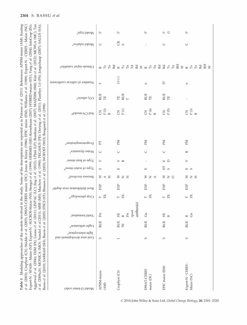
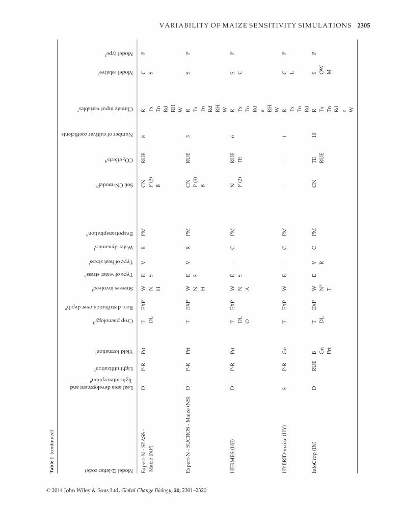
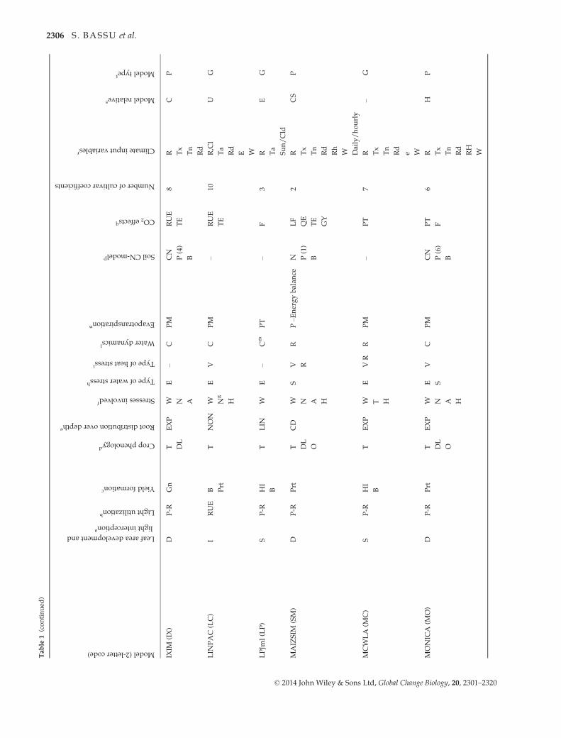
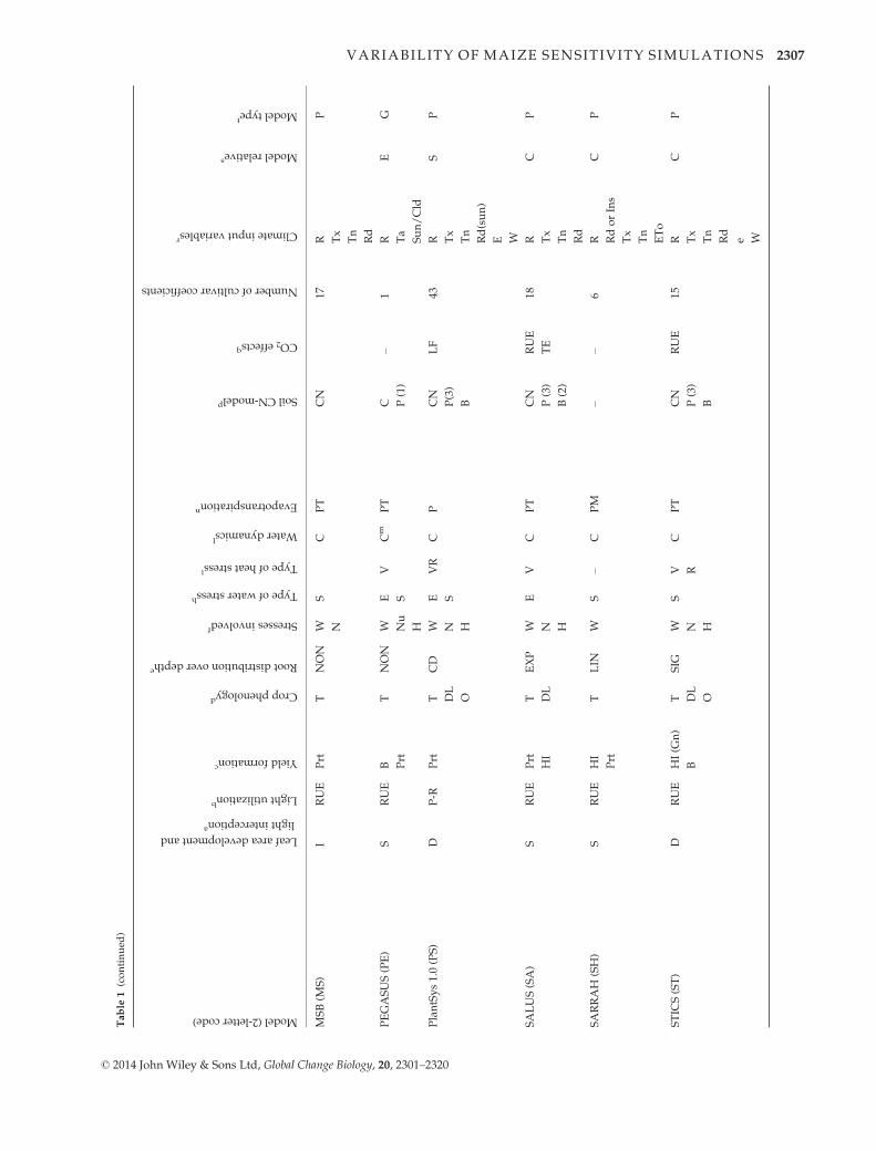
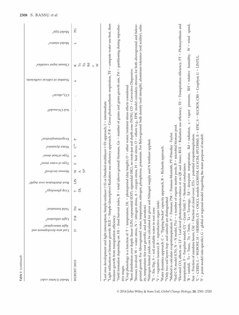
ment Project (AgMIP; Rosenzweig et al., 2013). Table 1 pre-

sents the major characteristics of the participating models,

including a reference for each of them and with details on

procedures used to simulate major processes (Palosuo et al.,

2011):

Phenology. Effects of life cycle drivers (temperature, photope-

riod), and/or stresses (e.g., McMaster & Wilhelm, 1997).

Growth. Radiation use efficiency (Monteith, 1977), transpira-

tion use efficiency (Tanner, 1981) or a leaf-level formulation of

photosynthesis and respiration (Farquhar et al., 1980; Von

Caemmerer, 2000). Most of the models simulate leaf area

dynamics dependent on crop phenological stage, following a

canopy-level (e.g., Jones & Kiniry, 1986) or a leaf-level (e.g.,

Lizaso et al., 2011) description.

Yield formation. Harvest index approach, dry matter alloca-

tion to the different organs, or grain number per unit of bio-

mass approach.

Water dynamics. Simplified ‘tipping bucket’ capacity

approach or a detailed Richards-type approach for infiltration

and redistribution of water in the soil. For evapotranspiration,

available methods varied and are indicated in Table 1. For

transpiration, limitations of soil and plant water potential or

soil water content are considered.

Nitrogen dynamics. Modules calculate soil and/or plant

nitrogen balance.

Simulations of each model were run by scientists already

experienced in the use of that particular model. Because most

models do not account for the effect of pests, and because the

impacts of climate on the biotic factors directly, were not con-

sidered here, this capability was disabled in all simulations.

Four models have no CO2 function (Sarra-H, Expert-ceres

maize, Wofost, and Pegasus). The same input data were pro-

vided to each modeler (soil, weather series, crop management,

see below for the details). All outputs were generated using

the same protocol, and submitted to an agreed upon group of

scientists that coordinated and centralized input and output

processing.

Data for model evaluation

Sites and weather. Four sentinel sites representing important

pedo-climatic zones of maize production were selected for

model intercomparison. The four sites were: Lusignan, France

(46.25°N; 00.07°E; 150 m elevation); Ames, Iowa, USA

(42.01°N; 93.45°W; 329 m elevation); Rio Verde, Brazil

(17.52°S; 51.43°W; 731 m elevation), and Morogoro, Tanzania

© 2014 John Wiley & Sons Ltd, Global Change Biology, 20, 2301–2320

VARIABILITY OF MAIZE SENSITIVITY SIMULATIONS 2303

Table

1Modelingap

proaches

ofthemodelsinvolved

inthestudy.Someofthedescriptionsarereported

asin

Palosu

oet

al.(201

1).Referen

ces:APSIM

-maize

(AM);Keating

etal.(200

3);CropSyst

(CS);St€ ockle

etal.(200

3);DSSAT-C

ERESmaize

(DC);Jones

&Kiniry(198

6);EPIC

maize

(EM);W

illiam

set

al.(198

9);Expert-N

-CERES-Maize

(NC)

Expert-N

-SPASS-Maize

(NP);Expert-N

-SUCROS-M

aize

(NS);Stenger

etal.(199

9);HERMES(H

E);Kersebau

m(200

7);HYBRID

-maize

(HY);Yan

get

al.(200

4);InfoCrop(IN);

Aggarwal

etal.(200

6);IXIM

(IX);Lizasoet

al.(201

1);LIN

PAC

(LC);Jinget

al.(201

2);LPJm

l(LP);Bondeauet

al.(200

7);MAIZSIM

(SM);Kim

etal.(201

2);MCW

LA

(MC);Tao

etal.(200

9a,b);MONIC

A(M

O);Nen

del

etal.(20

11);MSB(M

S);Much

ow

etal.(199

0);PEGASUS(PE);Derynget

al.(201

1);PlantSys1.0(PS);Jongschaa

p(200

7);SALUS(SA);

Basso

etal.(20

10);SARRAH

(SH);Baronet

al.(20

05);STIC

S(ST);Brissonet

al.(20

03);W

OFOST(W

O);Boogaa

rdet

al.(19

98)

Model(2-lettercode)

Leafareadevelopmentand

lightinterceptiona

Lightutilizationb

Yieldformationc

Cropphenologyd

Rootdistributionoverdepthe

Stressesinvolvedf

Typeofwaterstressh

Typeofheatstressi

Waterdynamicsl

Evapotranspirationn

SoilCN‐modelp

CO2effectsq

Numberofcultivarcoefficients

Climateinputvariablesr

Modelrelatives

Modeltypet

APSIM

-maize

(AM)

SRUE

Prt

T DL

EXP

W A H

SV

CPT

CN

P(3)

B

RUE

TE

5R Tx

Tn

Rd

CP

CropSyst

(CS)

IRUE

TE

HI

B Prt

(post

anthesis)

T DL

EXP

W N H

EV R

CPM

CN

P(1)

TE

RUE

T

13(+)

R Tx

Tn

Td

Rd

W

CR

S

P

DSSAT-C

ERES

maize

(DC)

SRUE

Gn

T DL

EXP

W N A

E–

CPM

CN

P(4)

B

RUE

TE

6R Tx

Tn

Rd

–P

EPIC

maize

(EM)

SRUE

HI

B

T DL

EXP

W N O

ET

S

E D

CPM

CN

P(5)

RUE

TE

57Rd

Tx

Tn

RH

W

CP G

Expert-N

-CERES-

Maize

(NC)

SRUE

B Gn

T DL

EXP

W N H

E S

VR

PM

CN

P(3)

B

–6

R Tx

Tn

Rd

RH

W

CP

© 2014 John Wiley & Sons Ltd, Global Change Biology, 20, 2301–2320

2304 S . BASSU et al.

Table

1(continued

)

Model(2-lettercode)

Leafareadevelopmentand

lightinterceptiona

Lightutilizationb

Yieldformationc

Cropphenologyd

Rootdistributionoverdepthe

Stressesinvolvedf

Typeofwaterstressh

Typeofheatstressi

Waterdynamicsl

Evapotranspirationn

SoilCN‐modelp

CO2effectsq

Numberofcultivarcoefficients

Climateinputvariablesr

Modelrelatives

Modeltypet

Expert-N

-SPASS-

Maize

(NP)

DP-R

Prt

T DL

EXP

W N H

E S

VR

PM

CN

P(3)

B

RUE

8R Tx

Tn

Rd

RH

W

C S

P

Expert-N

-SUCROS-Maize

(NS)

DP-R

Prt

TEXP

W N H

E S

VR

PM

CN

P(3)

B

RUE

3R Tx

Tn

Rd

RH

W

SP

HERMES(H

E)

DP-R

Prt

T DL

O

EXP

W N A

E S

–C

PM

N P(2)

RUE

TE

6R Tx

Tn

Rd

e RH

W

S C

P

HYBRID

-maize

(HY)

SP-R

Gn

TEXP

WE

–C

PM

––

1R Tx

Tn

Rd

C L

P

InfoCrop(IN)

DRUE

B Gn

Prt

T DL

EXP

W Ng

T

EV R

CPM

CN

TE

RUE

10R Tx

Tn

Rd

e W

S OW

M

P

© 2014 John Wiley & Sons Ltd, Global Change Biology, 20, 2301–2320

VARIABILITY OF MAIZE SENSITIVITY SIMULATIONS 2305

Table

1(continued

)

Model(2-lettercode)

Leafareadevelopmentand

lightinterceptiona

Lightutilizationb

Yieldformationc

Cropphenologyd

Rootdistributionoverdepthe

Stressesinvolvedf

Typeofwaterstressh

Typeofheatstressi

Waterdynamicsl

Evapotranspirationn

SoilCN‐modelp

CO2effectsq

Numberofcultivarcoefficients

Climateinputvariablesr

Modelrelatives

Modeltypet

IXIM

(IX)

DP-R

Gn

T DL

EXP

W N A

E–

CPM

CN

P(4)

B

RUE

TE

8R Tx

Tn

Rd

CP

LIN

PAC(LC)

IRUE

B Prt

TNON

W Ng

H

EV

CPM

–RUE

TE

10R,Cl

Ta

Rd

E W

UG

LPJm

l(LP)

SP-R

HI

B

TLIN

WE

–Cm

PT

–F

3R Ta

Sun/Cld

EG

MAIZSIM

(SM)

DP-R

Prt

T DL

O

CD

W N A H

SV R

RP–E

nergybalan

ceN P(1)

B

LF

QE

TE

GY

2R Tx

Tn

Rd

Rh

W Daily/hourly

CS

P

MCW

LA

(MC)

SP-R

HI

B

TEXP

W T H

EVR

RPM

–PT

7R Tx

Tn

Rd

e W

–G

MONIC

A(M

O)

DP-R

Prt

T DL

O

EXP

W N A H

E S

VC

PM

CN

P(6)

B

PT

F

6R Tx

Tn

Rd

RH

W

HP

© 2014 John Wiley & Sons Ltd, Global Change Biology, 20, 2301–2320

2306 S . BASSU et al.

Table

1(continued

)Model(2-lettercode)

Leafareadevelopmentand

lightinterceptiona

Lightutilizationb

Yieldformationc

Cropphenologyd

Rootdistributionoverdepthe

Stressesinvolvedf

Typeofwaterstressh

Typeofheatstressi

Waterdynamicsl

Evapotranspirationn

SoilCN‐modelp

CO2effectsq

Numberofcultivarcoefficients

Climateinputvariablesr

Modelrelatives

Modeltypet

MSB(M

S)

IRUE

Prt

TNON

W N

SC

PT

CN

17R Tx

Tn

Rd

P

PEGASUS(PE)

SRUE

B Prt

TNON

W Nu

H

E S

VCm

PT

C P(1)

–1

R Ta

Sun/Cld

EG

PlantSys1.0(PS)

DP-R

Prt

T DL

O

CD

W N H

E S

VR

CP

CN

P(3)

B

LF

43R Tx

Tn

Rd(sun)

E W

SP

SALUS(SA)

SRUE

Prt

HI

T DL

EXP

W N H

EV

CPT

CN

P(3)

B(2)

RUE

TE

18R Tx

Tn

Rd

CP

SARRAH

(SH)

SRUE

HI

Prt

TLIN

WS

–C

PM

––

6R RdorIns

Tx

Tn

ETo

CP

STIC

S(ST)

DRUE

HI(G

n)

B

T DL

O

SIG

W N H

SV R

CPT

CN

P(3)

B

RUE

15R Tx

Tn

Rd

e W

CP

© 2014 John Wiley & Sons Ltd, Global Change Biology, 20, 2301–2320

VARIABILITY OF MAIZE SENSITIVITY SIMULATIONS 2307

Table

1(continued

)

Model(2-lettercode)

Leafareadevelopmentand

lightinterceptiona

Lightutilizationb

Yieldformationc

Cropphenologyd

Rootdistributionoverdepthe

Stressesinvolvedf

Typeofwaterstressh

Typeofheatstressi

Waterdynamicsl

Evapotranspirationn

SoilCN‐modelp

CO2effectsq

Numberofcultivarcoefficients

Climateinputvariablesr

Modelrelatives

Modeltypet

WOFOST(W

O)

DP-R

Prt

B

T DL

LIN

W A Ng

SV

Cm

P–

–6

R Tx

Tn

Rd

e W

LPG

aLeafarea

dev

elopmen

tan

dlightintercep

tion;Sim

ple-unilay

er(=S)orDetailed-m

ultilay

er(=D)ap

proach;I=interm

ediate.

bLightutiliza

tionorbiomassgrowth:RUE=Sim

ple

(descriptive)

Rad

iationuse

efficien

cyap

proach,P

-R=Gross

photosynthesis–respiration,TE=compute

water

use

first,then

biomassgrowth

from

tran

spirationefficien

cy.

cYield

form

ationdep

endingon:HI=fixed

harvestindex,B=total(above-ground)biomass,Gn=number

ofgrainsan

dgrain-growth

rate,Prt

=partitioningduringreproduc-

tivestag

es.

dCropphen

ologyisafunctionof:T=temperature,DL=photoperiod(day

length);O

=other

water/nutrientstress

effectsconsidered

.eRootdistributionover

dep

th:linear(LIN

),exponen

tial

(EXP),sigmoidal

(SIG

),noroots-just

soildep

thzo

ne(N

ON),CD

=ConvectiveDispersive.

f Stressesinvolved

:W

=water

stress,N

=nitrogen

stress,A

=oxygen

stress,H

=heatstress;O

=others(e.g.,EPIC

model

considersstresses

forboth

aboveg

roundan

dbelow-

groundgrowth.ForAboveg

round:water,temperature,nitrogen

,phosp

horus,potassium.ForBelowground:bulk

den

sity

(soilstrength),aluminum

tolerance

(soilacidity),salin-

ity,temperature

(forrootgrowth),an

dsoilaeration).

gNitrogen

-lim

ited

yieldscanbecalculatedforgiven

soilNitrogen

supply

andN

fertilizer

applied

.hE=Eta/Etp,S=soilav

ailable

water

inrootzo

ne.

i V=veg

etative(source),R

=reproductiveorgan

(sink).

l Water

dynam

icsap

proach:C

=‘Tippingbucket’capacityap

proach,R

=Richardsap

proach.

mOnly

twosoillayers(top-an

dsu

bsoil)aredistinguished

.nMethodto

calculate

evap

otran

spiration:P=Pen

man

;PM

=Pen

man

-Monteith,PT=Priestley

–Tay

lor.

pSoilC-N

model

(CN),N

=N

model,P(x)=xnumber

oforgan

icmatterpools,B=microbialbiomasspool.

qElevated

CO

2effectson:LF=Leaf-level

photosynthesis-rubisco

oronQEan

dAmax

;RUE=Rad

iationuse

efficien

cy,TE=Transp

irationefficien

cy,PT=Photosynthesis

and

tran

spiration,F=Farquhar

model,GY

=Grain

Yield;T=Stomatal

conductan

ce.

r R=rainfall,

Tx=Tmax

,Tn=Tmin,

Ta=Tav

erag

e,Td=dew

point

temperature,

Rd=radiation,

e=vap

or

pressure,

RH

=relative

humidity,

W=wind

speed,

Sun=Fractionofsu

nsh

inehours,Cld

=Fractionofcloudcover,ETo=potential

evap

otran

spiration.

s C=CERES,L=W

OFOST,H

=HERMES,CS=CSGCLmodels(G

OSSYM,GLYCIM

,SPUDSIM

),E=EPIC

,S=SUCROS,CRS=CropSyst;U

=LIN

TUL.

t P=pointmodel

(site-sp

ecific),G

=global

orregional

model

(reg

ardingthemainpurpose

ofmodel).

© 2014 John Wiley & Sons Ltd, Global Change Biology, 20, 2301–2320

2308 S . BASSU et al.

(06.50°S; 37.39°E; 500 m elevation). Basic characteristics of the

study sites are summarized in Table 2.

According to the FAO classification, the soils are Cambisol

in Lusignan, Gleysol in Ames, Geri-Gibbsic Ferralsol in Rio

Verde, and Haplic Arenosol in Morogoro. Daily solar radia-

tion, maximum and minimum air temperature (2 m), and

precipitation for the 1980–2010 historical baseline climates

were provided to crop modeling groups for all sites. Available

daily measurements of surface wind speed, air humidity (dew

point temperature, vapor pressure, and relative humidity at

the time of day of maximum temperatures) were provided.

Where these variables were not measured, they were esti-

mated from the NASA Modern Era Retrospective-Analysis for

Research and Applications (MERRA; Rienecker et al., 2011).

At Lusignan, France, the mean annual rainfall (1980–2010)

is 819 mm, of which 28% falls between May and August.

Ames, USA has a continental climate with temperature

extremes of both hot and cold, and long-term mean annual

precipitation (1980–2010) of 886 mm, 54% of which falls from

May through August. Rio Verde, Brazil is the wettest location

with a seasonal distribution of precipitation. The mean annual

rainfall (1980–2010) is 1645 mm, with the rainy season extend-

ing from October through April. Morogoro, Tanzania is the

warmest location with monthly mean maximum and mini-

mum temperatures varying between 35 and 14 °C and long-

term annual rainfall of 828 mm, with 90% falling from

November through May.

Management. A one-year experiment at each location formed

the basis of the comparison of observed and modeled data for

the four locations. The field experiments were carried out

from May to October in 1996 in Lusignan, from May to Sep-

tember in 2010 in Ames, from November to February in 2003–

2004 in Rio Verde, and from November to January in 2009–

2010 in Morogoro. Experiments were conducted according to

the local practices for each region (Table 3). Lusignan and

Morogoro were the two irrigated sites. Nitrogen fertilizer was

not applied in Rio Verde because sufficient N was released by

organic matter mineralization.

Crop measurements. Measured crop data for each site con-

sisted of phenology (emergence, flowering, and maturity

dates) and intensive in-season time-series information [soil

water content, leaf area index (LAI), crop biomass] as well as

end-of-season yield components. Details on the experiments

are reported for Lusignan, France (Tayot et al.,1999;

Brisson et al., 2002), Ames, USA (Bortolon L & Hatfield JL,

unpublished data), Rio Verde, Brazil (Maltas et al., 2007, 2009),

and Morogoro, Tanzania (Bobert J, Festo R, Kersebaum KC,

Kashaigili JJ, Tumbo S & Mahoo H, unpublished data).

Low level calibration simulation procedures. In regional

studies, many inputs required by crop models are often not

available. To examine the effect of the level of detail in the

input information upon the model response to climatic factors,

we provided two levels of calibration information, a low (L)

and a high (H) level. For level L, only soil, management

inputs, and crop phenology data were provided. Models were

run with standard soil initial conditions such as prior crop res-

idue type depending on the previous crop (legumes or cereals)

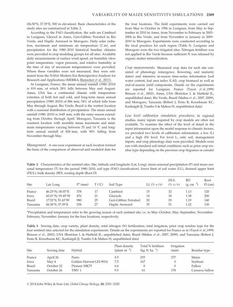
Table 2 Characteristics of the sentinel sites. Site, latitude and longitude (Lat, Long), mean seasonal precipitation (P) and mean sea-

sonal temperature (T) for the period 1980–2010, soil type (FAO classification), lower limit of soil water (LL), drained upper limit

(DUL), bulk density (BD), rooting depth (Root D)

Site Lat; Long Pa (mm) T (°C) Soil Type LL (% v/v)

DUL

(% v/v)

BD

(g cm�3)

Root

D (cm)

France 46.25°N; 00.07°E 378 17 Cambisol 15 32 1.13 120

Iowa 42.01°N; 93.45°W 476 21 Gleysols 14 34 1.38 200

Brazil 17.52°S; 51.43°W 980 25 Geri-Gibbsic Ferralsol 20 29 1.19 140

Tanzania 06.50°S; 37.39°E 258 27 Haplic Arenosol 35 51 1.22 130

aPrecipitation and temperature refer to the growing season of each sentinel site, i.e. to May–October, May–September, November–

February, November–January for the four locations, respectively.

Table 3 Sowing date, crop variety, plant density, total nitrogen (N) fertilization, total irrigation, prior crop residue type for the

four sentinel sites selected for the simulation experiments. Details on the experiments are reported for France as in (Tayot et al.,1999;

Brisson et al., 2002), USA (Bortolon L & Hatfield JL, unpublished data), Brazil (Maltas et al., 2007, 2009), and Tanzania (Bobert J,

Festo R, Kersebaum KC, Kashaigili JJ, Tumbo S & Mahoo H, unpublished data)

Site Sowing date Hybrid

Plant density

(plant m�2)

Total N fertilizer

(kg N ha�1)

Irrigation

(mm) Residue type

France April 26 Furio 9.5 255 377 Maize

Iowa May 4 Golden Harvest GH-9014 7.5 167 0 Soybean

Brazil October 22 Pioneer 30K75 6.6 0 0 Fallow

Tanzania October 26 TMV 1 9.5 61 178 Cassava/fallow

© 2014 John Wiley & Sons Ltd, Global Change Biology, 20, 2301–2320

VARIABILITY OF MAIZE SENSITIVITY SIMULATIONS 2309

and using the soil organic carbon of the prevailing soil type of

the region. The initial soil water content was set at field capac-

ity (Lusignan, Ames) or wilting point (Rio Verde, Morogoro,)

according to the general rainfall pattern of each location. Crop

field management (sowing date and depth, plant density,

nitrogen fertilization dates and amounts, irrigation schedule

when applied), per-layer soil characteristics (wilting point,

field capacity, saturation, bulk density, pH, and organic car-

bon and nitrogen), and local maximum observed rooting

depth were also provided. Thus, simulations at level L were

run at each site [for a single year (calibration) and for a 30-

year-baseline and sensitivity tests (as described below)] using

only the above described input information, with no parame-

ter adjustment other than setting the time to anthesis and time

to maturity observed in each region.

High level calibration simulation procedures. After the L

level input simulations were completed, additional crop and

soil information (H level) was supplied to each modeling

group. The complete information provided included the

actual soil initial conditions (water, nitrate, ammonium), and

time series of above-ground biomass, LAI, soil water and

nitrogen contents, and plant nitrogen. Soil and plant N infor-

mation were not available for the Tanzania site. It was

requested that each modeling group adjust model parameters

(especially those depending on the cultivar) to improve the

simulations based on the observed data, using whatever tech-

niques they normally use and documenting the changes. For

that purpose, each modeler was requested to send a report on

changes made in the values of parameters and what logic was

followed. Twenty-one groups completed the full assessment

of that step. For the L simulation, modelers adjusted cultivar

parameters of their previously simulated hybrids, to match

the provided phenology. In the H simulation phase, finer

adjustment of phenology and plant traits such as final leaf

length, leaf number, specific leaf area (SLA) were made, if

applicable. Modelers never changed parameters linked to pho-

tosynthesis or RUE, or any other temperature-sensitive rela-

tionships. Soil parameters (relationships of soil water potential

and conductivity to soil water content) were also adjusted to

match the initial conditions. Some simpler models designed

for larger scales had less flexibility and were largely unaltered,

except for phenology. The given cultivar was different at each

site, so the cultivar parameter sets differed by site. Conse-

quently, the adjustments for the H phase were larger because

the models had never been used before at those sites. After

parameters were adjusted, the models were run with the

specific single year experiment at each site.

Climatic sensitivity analyses using modified 30-yearclimate series

To study simulated responses to climate change factors tem-

perature and [CO2], models with parameters adjusted using H

input level information were run for a 30-year-baseline and

several modified 30-year weather files for the four locations.

The baseline weather series were modified by changing

daily maximum and minimum temperatures (�3, 0, +3, +6

and +9 °C). Modeled responses were also compared under

different levels of [CO2] (360, 450, 540, 630 and

720 lmol mol�1). The temperature and [CO2] modifications

were considered both in single factor series and in several

combinations for the High input calibration simulations. As

summarized in Table 4, simulations for the Low input case

were limited to only the single factor variation in temperature

and [CO2], with the goal of understanding how calibration

influenced model sensitivity to temperature and [CO2]. Simu-

lated model response to [CO2] is presented only for the 15

models describing explicitly [CO2] effects, out of the models

that concluded the High inputs simulations.

Simulation protocol

Simulation experiments were carried out for the 1980–2009

time series (30 planting seasons) for the baseline and the vari-

ous modified 30-year weather data sets for the four locations.

For each year, initial soil conditions were reset to those used

for level L or for level H. The LPJmL model was run continu-

ously with a 100-year spin up just to set the initial organic

matter compartments of soils at each site. After this goal was

achieved, it was run as the other models. Resetting the soil ini-

tial conditions eliminated any carry-over of water, nitrogen,

or a change in soil organic matter. For the irrigated locations

(Lusignan, France, and Morogoro, Tanzania), automatic irriga-

tion was triggered when the soil water content within the top

50 cm depth dropped under 60% of the plant available water.

Analysis of model responses to temperature and [CO2]

Comparative effects of single weather variables and interac-

tions on model results (H information level averages over

30-year initial or modified baseline simulated yield, biomass

Table 4 Levels of CO2 and temperature factors simulated for

each location for the low and high input information simula-

tions. Temperature factor levels applied to maximum and

minimum daily temperatures of the 30-year-baseline weather

data

Low level input High level input

360 ppm �3 °C 360 ppm �3 °C360 ppm 0 °C 360 ppm 0 °C360 ppm +3 °C 360 ppm +3 °C360 ppm +6 °C 360 ppm +6 °C360 ppm +9 °C 360 ppm +9 °C450 ppm 0 °C 450 ppm 0 °C540 ppm 0 °C 540 ppm 0 °C630 ppm 0 °C 630 ppm 0 °C720 ppm 0 °C 720 ppm 0 °C

540 ppm +3 °C540 ppm +6 °C540 ppm +9 °C720 ppm +3 °C720 ppm +6 °C720 ppm +9 °C

© 2014 John Wiley & Sons Ltd, Global Change Biology, 20, 2301–2320

2310 S . BASSU et al.

and transpiration) were evaluated with Analysis of Variance

for each site. For that analysis, three levels of [CO2], four tem-

perature variations above the baseline, and models were con-

sidered fixed effects with 2, 3, and 18 degrees of freedoms,

respectively. All interactions were tested. Climate factors and

model effects were highly significant at all sites. So were

interactions between temperature and CO2 except in Lusignan

(P < 0.08). Graphical analyses were also used for model inter-

comparison by plotting medians and variability distributions

(box-plots) of simulated outputs and used to estimate the

responses of yield to T and CO2.

Results

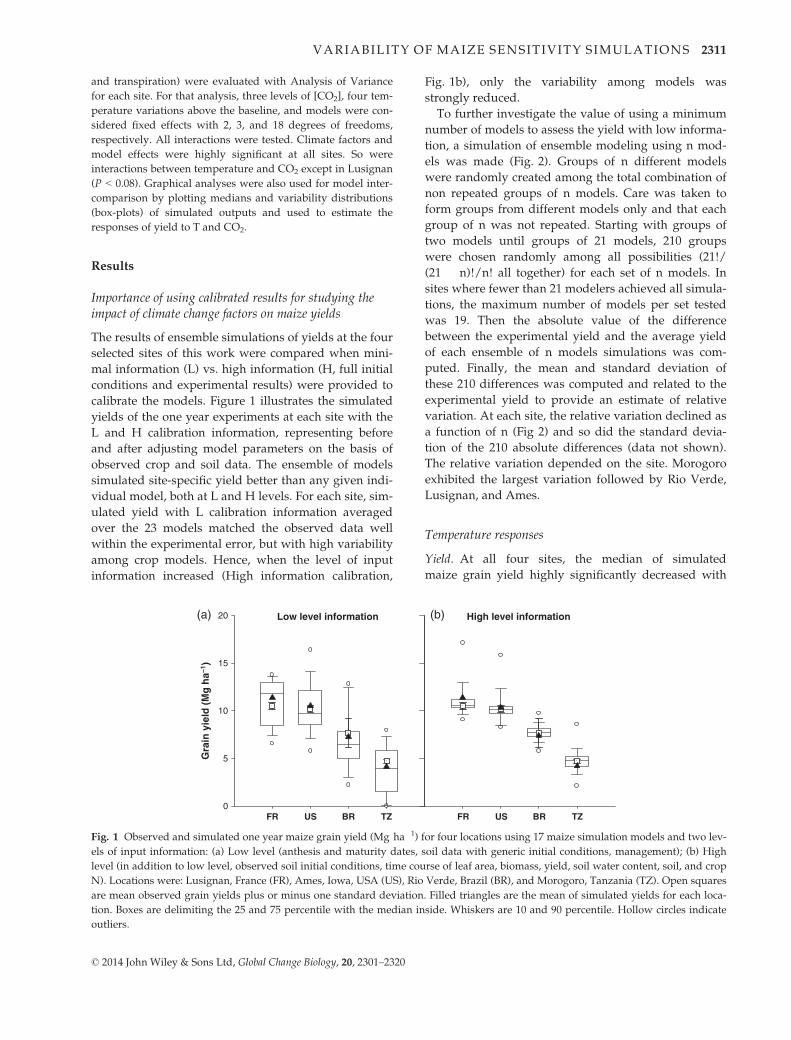
Importance of using calibrated results for studying theimpact of climate change factors on maize yields

The results of ensemble simulations of yields at the four

selected sites of this work were compared when mini-

mal information (L) vs. high information (H, full initial

conditions and experimental results) were provided to

calibrate the models. Figure 1 illustrates the simulated

yields of the one year experiments at each site with the

L and H calibration information, representing before

and after adjusting model parameters on the basis of

observed crop and soil data. The ensemble of models

simulated site-specific yield better than any given indi-

vidual model, both at L and H levels. For each site, sim-

ulated yield with L calibration information averaged

over the 23 models matched the observed data well

within the experimental error, but with high variability

among crop models. Hence, when the level of input

information increased (High information calibration,

Fig. 1b), only the variability among models was

strongly reduced.

To further investigate the value of using a minimum

number of models to assess the yield with low informa-

tion, a simulation of ensemble modeling using n mod-

els was made (Fig. 2). Groups of n different models

were randomly created among the total combination of

non repeated groups of n models. Care was taken to

form groups from different models only and that each

group of n was not repeated. Starting with groups of

two models until groups of 21 models, 210 groups

were chosen randomly among all possibilities (21!/(21 � n)!/n! all together) for each set of n models. In

sites where fewer than 21 modelers achieved all simula-

tions, the maximum number of models per set tested

was 19. Then the absolute value of the difference

between the experimental yield and the average yield

of each ensemble of n models simulations was com-

puted. Finally, the mean and standard deviation of

these 210 differences was computed and related to the

experimental yield to provide an estimate of relative

variation. At each site, the relative variation declined as

a function of n (Fig 2) and so did the standard devia-

tion of the 210 absolute differences (data not shown).

The relative variation depended on the site. Morogoro

exhibited the largest variation followed by Rio Verde,

Lusignan, and Ames.

Temperature responses

Yield. At all four sites, the median of simulated

maize grain yield highly significantly decreased with

Low level information

Gra

in y

ield

(M

g h

a–1)

0

5

10

15

20(a) (b) High level information

FR US BR TZ FR US BR TZ

Fig. 1 Observed and simulated one year maize grain yield (Mg ha�1) for four locations using 17 maize simulation models and two lev-

els of input information: (a) Low level (anthesis and maturity dates, soil data with generic initial conditions, management); (b) High

level (in addition to low level, observed soil initial conditions, time course of leaf area, biomass, yield, soil water content, soil, and crop

N). Locations were: Lusignan, France (FR), Ames, Iowa, USA (US), Rio Verde, Brazil (BR), and Morogoro, Tanzania (TZ). Open squares

are mean observed grain yields plus or minus one standard deviation. Filled triangles are the mean of simulated yields for each loca-

tion. Boxes are delimiting the 25 and 75 percentile with the median inside. Whiskers are 10 and 90 percentile. Hollow circles indicate

outliers.

© 2014 John Wiley & Sons Ltd, Global Change Biology, 20, 2301–2320

VARIABILITY OF MAIZE SENSITIVITY SIMULATIONS 2311

temperature increase above current temperature levels

(Fig. 3). The decrease in yield with an increase in tem-

perature from 0 to +9 °C across 19 crop models was

approximately linear and the median of models

decreased from 9.8 to 6.3 Mg ha�1 at Lusignan (France),

from 9.4 to 4.3 Mg ha�1 at Ames (USA), from 7.5 to 2.4

Mg ha�1at Rio Verde (Brazil), and from 5.2 to 1.8

Mg ha�1 at Morogoro (Tanzania). This corresponded to

a relative yield change of �4.5, �6.0, �7.8 and �7.1%

per °C at the four sites, respectively. With only few

exceptions, the 19 maize models with High inputs sim-

ulations generally agreed on a decline in yield with

warmer weather. The models varied in magnitude of

yield reduction with temperature increase, with 50% of

models having sensitivity between �3.5% and �5.2%

per °C in Lusignan, �4.8% and �6.6% per °C in Ames,

�6.4% and �8.3% per °C in Rio Verde, and �3.4% and

�9.8% per °C in Morogoro. The other models outside

of this 50% had a lower or higher response ranging

from no response up to double response with respect to

Number of models averaged

0 2 4 6 8 10 12 14 16 18 20Rel

ativ

e va

riat

ion

bet

wee

n a

vera

ge

of

n m

od

els

and

mea

sure

d y

ield

0.00

0.05

0.10

0.15

0.20

0.25

0.30

0.35Morogoro, TZ Lusignan, FRRio Verde, BRAmes, US

Fig. 2 Relative variation between observed and average yield

simulated with n randomly selected models among 19 at 4

world sites, as a function of n. Each set of n models was com-

posed with the requirement that each model of the set was used

only once in a given set, and that all models were equally repre-

sented in the 210 sets.

Temperature change (°C)

0

5

10

15

–3 0 3 6 9 –3 0 3 6 9

Gra

in y

ield

(M

g h

a–1)

0

5

10

15

20

(a) Lusignan, France (b) Ames, USA

(c) Rio Verde, Brazil (d) Morogoro, Tanzania

Fig. 3 Temperature effect on 30-year grain yield (Mg ha�1) simulated by 19 models at Lusignan, France (a), Ames, USA (b), Rio Verde,

Brazil (c), Morogoro, Tanzania (d). Maximum and minimum temperatures were decreased every day by 3 °C, or increased by 0, 3, 6,

and 9 °C. Box-plot description is similar to Fig. 1 except for the absence of measured and mean values. Mean baseline temperatures

during the growing cycle were 17, 21, 25, and 27 °C in Lusignan, Ames, Rio Verde, and Morogoro, respectively.

© 2014 John Wiley & Sons Ltd, Global Change Biology, 20, 2301–2320

2312 S . BASSU et al.

the median relative yield change. The variation among

absolute yield simulations as shown by the box-and-

whisker plot was scarcely different as temperature

increased.

However, at the cooler sites (Lusignan and Ames,

the high-latitude sites), a lower temperature (�3 °Cbelow baseline) resulted in lower simulated grain

yield, probably because simulated biomass produc-

tion rates decreased in the models, and crop maturity

was prolonged and abruptly ended in the fall. At the

warmer locations (the low-latitude sites), the 3 °Ccooler temperature increased simulated yields (by

6.0% and 1.2% per °C in Rio Verde and Morogoro,

respectively), suggesting that these sites are already

warmer than the optimal growing climate (See Fig-

ures S1 and S2 in supplemental material for individ-

ual crop models response as a function of the 30-year

seasonal temperature). The variability in responses

among models increased with the �3 °C temperature

scenario, especially at cool locations (Figure S2 in

supplemental).

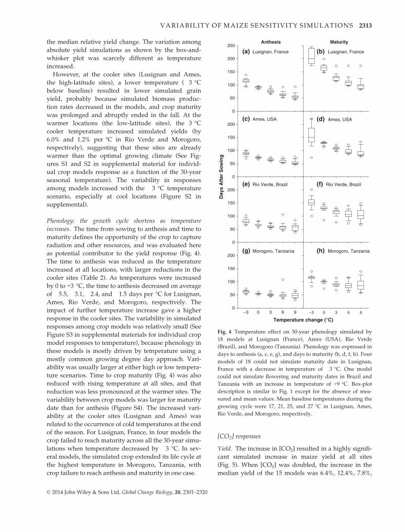
Phenology: the growth cycle shortens as temperature

increases. The time from sowing to anthesis and time to

maturity defines the opportunity of the crop to capture

radiation and other resources, and was evaluated here

as potential contributor to the yield response (Fig. 4).

The time to anthesis was reduced as the temperature

increased at all locations, with larger reductions in the

cooler sites (Table 2). As temperatures were increased

by 0 to +3 °C, the time to anthesis decreased on average

of �5.5, �3.1, �2.4, and �1.5 days per °C for Lusignan,

Ames, Rio Verde, and Morogoro, respectively. The

impact of further temperature increase gave a higher

response in the cooler sites. The variability in simulated

responses among crop models was relatively small (See

Figure S3 in supplemental materials for individual crop

model responses to temperature), because phenology in

these models is mostly driven by temperature using a

mostly common growing degree day approach. Vari-

ability was usually larger at either high or low tempera-

ture scenarios. Time to crop maturity (Fig. 4) was also

reduced with rising temperature at all sites, and that

reduction was less pronounced at the warmer sites. The

variability between crop models was larger for maturity

date than for anthesis (Figure S4). The increased vari-

ability at the cooler sites (Lusignan and Ames) was

related to the occurrence of cold temperatures at the end

of the season. For Lusignan, France, in four models the

crop failed to reach maturity across all the 30-year simu-

lations when temperature decreased by �3 °C. In sev-

eral models, the simulated crop extended its life cycle at

the highest temperature in Morogoro, Tanzania, with

crop failure to reach anthesis and maturity in one case.

[CO2] responses

Yield. The increase in [CO2] resulted in a highly signifi-

cant simulated increase in maize yield at all sites

(Fig. 5). When [CO2] was doubled, the increase in the

median yield of the 15 models was 6.4%, 12.4%, 7.8%,

MaturityAnthesis

–3 0 3 6 9 –3 0 3 6 9

Day

s A

fter

So

win

g

0

50

100

150

200

0

50

100

150

200

0

50

100

150

200

0

50

100

150

200

250

(a) Lusignan, France (b) Lusignan, France

(c) Ames, USA (d) Ames, USA

(e) Rio Verde, Brazil

(g) Morogoro, Tanzania (h) Morogoro, Tanzania

(f) Rio Verde, Brazil

Temperature change (°C)

Fig. 4 Temperature effect on 30-year phenology simulated by

18 models at Lusignan (France), Ames (USA), Rio Verde

(Brazil), and Morogoro (Tanzania). Phenology was expressed in

days to anthesis (a, c, e, g), and days to maturity (b, d, f, h). Four

models of 18 could not simulate maturity date in Lusignan,

France with a decrease in temperature of �3 °C. One model

could not simulate flowering and maturity dates in Brazil and

Tanzania with an increase in temperature of +9 °C. Box-plot

description is similar to Fig. 1 except for the absence of mea-

sured and mean values. Mean baseline temperatures during the

growing cycle were 17, 21, 25, and 27 °C in Lusignan, Ames,

Rio Verde, and Morogoro, respectively.

© 2014 John Wiley & Sons Ltd, Global Change Biology, 20, 2301–2320

VARIABILITY OF MAIZE SENSITIVITY SIMULATIONS 2313

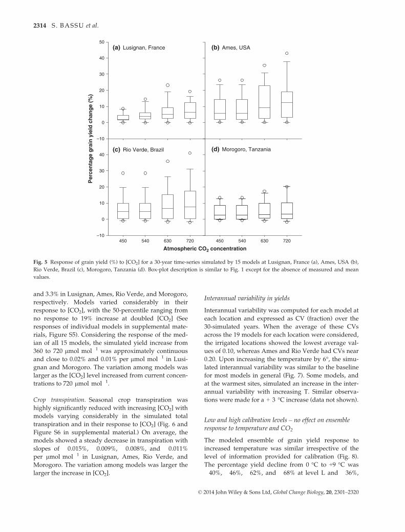
and 3.3% in Lusignan, Ames, Rio Verde, and Morogoro,

respectively. Models varied considerably in their

response to [CO2], with the 50-percentile ranging from

no response to 19% increase at doubled [CO2] (See

responses of individual models in supplemental mate-

rials, Figure S5). Considering the response of the med-

ian of all 15 models, the simulated yield increase from

360 to 720 lmol mol�1 was approximately continuous

and close to 0.02% and 0.01% per lmol mol�1 in Lusi-

gnan and Morogoro. The variation among models was

larger as the [CO2] level increased from current concen-

trations to 720 lmol mol�1.

Crop transpiration. Seasonal crop transpiration was

highly significantly reduced with increasing [CO2] with

models varying considerably in the simulated total

transpiration and in their response to [CO2] (Fig. 6 and

Figure S6 in supplemental material.) On average, the

models showed a steady decrease in transpiration with

slopes of �0.015%, �0.009%, �0.008%, and �0.011%

per lmol mol�1 in Lusignan, Ames, Rio Verde, and

Morogoro. The variation among models was larger the

larger the increase in [CO2].

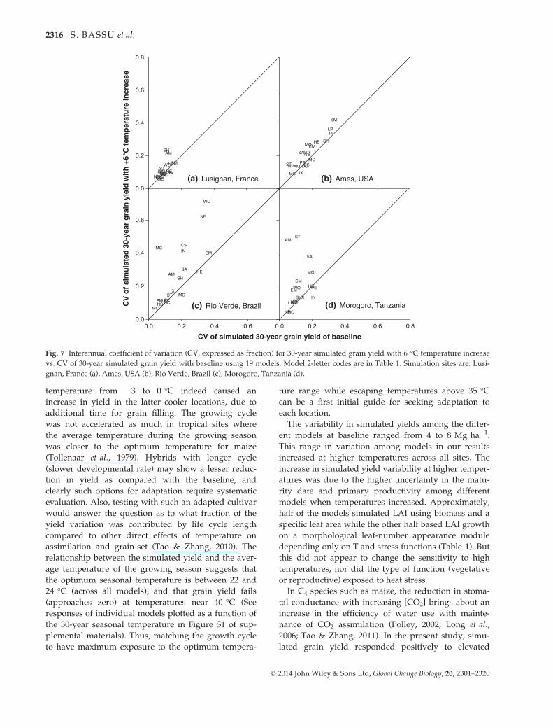
Interannual variability in yields

Interannual variability was computed for each model at

each location and expressed as CV (fraction) over the

30-simulated years. When the average of these CVs

across the 19 models for each location were considered,

the irrigated locations showed the lowest average val-

ues of 0.10, whereas Ames and Rio Verde had CVs near

0.20. Upon increasing the temperature by 6°, the simu-

lated interannual variability was similar to the baseline

for most models in general (Fig. 7). Some models, and

at the warmest sites, simulated an increase in the inter-

annual variability with increasing T. Similar observa-

tions were made for a + 3 °C increase (data not shown).

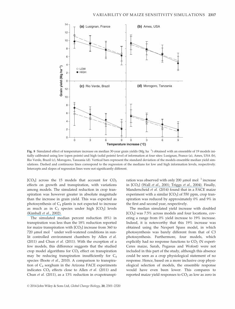
Low and high calibration levels – no effect on ensembleresponse to temperature and CO2

The modeled ensemble of grain yield response to

increased temperature was similar irrespective of the

level of information provided for calibration (Fig. 8).

The percentage yield decline from 0 °C to +9 °C was

�40%, �46%, �62%, and �68% at level L and �36%,

Atmospheric CO2 concentration450 540 630 720 450 540 630 720

Per

cen

tag

e g

rain

yie

ld c

han

ge

(%)

–10

0

10

20

30

40

–10

0

10

20

30

40

50(a) Lusignan, France (b) Ames, USA

(c) Rio Verde, Brazil (d) Morogoro, Tanzania

Fig. 5 Response of grain yield (%) to [CO2] for a 30-year time-series simulated by 15 models at Lusignan, France (a), Ames, USA (b),

Rio Verde, Brazil (c), Morogoro, Tanzania (d). Box-plot description is similar to Fig. 1 except for the absence of measured and mean

values.

© 2014 John Wiley & Sons Ltd, Global Change Biology, 20, 2301–2320

2314 S . BASSU et al.

�54%, �71%, and �65% at level H, respectively for

Lusignan, Ames, Rio Verde, and Morogoro. At each

location, the slope of the temperature response did not

vary between the L and H information. Neither did the

slope vary with location. Finally, the model response to

[CO2] was also not dependent on the level of calibration

information (data not shown).

Discussion

By comparing results from a large number of models in

four contrasting environments, our work expands the

previous efforts (e.g., Eitzinger et al. (2013) that only

evaluated a 2-week period of drought or elevated tem-

perature after anthesis on maize yield). Our simulations

hence explore and define more completely maize crop

responses to two major climate change factors (temper-

ature and CO2) with up to 23 maize simulation models.

The effect of rising temperatures on maize yield was

strongly negative. The common trend of models

simulations to accelerate phenology, especially anthesis

in response to temperature, largely explained the main

trends for reduction in the other variables studied

(biomass, yield and water use). These simulations were

conducted without attempting adaptive measures to

ameliorate the impact of higher temperatures, such as

changes in planting dates or maize cultivar life cycle

duration. Thus, these simulations provide an estimate

of the upper boundary of the expected average

decrease in maize yield at these locations and under

well-watered conditions.

Increased temperature shortened the length of the

growing cycle, decreasing opportunity to capture more

radiation and reducing total CO2 assimilation, and

reducing total biomass and grain yield as suggested by

previous studies (Long, 1991; Guere~na et al., 2001; Tao

& Zhang, 2011). Therefore, shorter life cycle of current

cultivars was a major contributor to reduced grain

yield, diminishing leaf area duration and hence, bio-

mass accumulation. Biomass production (data not

shown) was affected very similarly to grain yield. On

the contrary, the grain harvest index (data not shown)

was unaffected by temperature elevation in the 0–6 °Ctemperature range, except for some reductions at the

high (+6 °C or above at Morogoro) or the low tempera-

ture extremes (�3 °C in Lusignan and Ames). Raising

Per

cen

tag

e cr

op

tra

nsp

irat

ion

ch

ang

e (%

)

–40

–30

–20

–10

0

10

20

–40

–30

–20

–10

0

10

20

30(a) Lusignan, France (b) Ames, USA

(c) Rio Verde, Brazil (d) Morogoro, Tanzania

Atmospheric CO2 concentration

450 540 630 720 450 540 630 720

Fig. 6 [CO2] effect on the percentage change in 30-year average crop transpiration (%) simulated by 15 models at Lusignan, France (a),

Ames, USA (b), Rio Verde, Brazil (c), Morogoro, Tanzania (d). Box-plot description is similar to Fig. 1 except for the absence of mea-

sured and mean values.

© 2014 John Wiley & Sons Ltd, Global Change Biology, 20, 2301–2320

VARIABILITY OF MAIZE SENSITIVITY SIMULATIONS 2315

temperature from �3 to 0 °C indeed caused an

increase in yield in the latter cooler locations, due to

additional time for grain filling. The growing cycle

was not accelerated as much in tropical sites where

the average temperature during the growing season

was closer to the optimum temperature for maize

(Tollenaar et al., 1979). Hybrids with longer cycle

(slower developmental rate) may show a lesser reduc-

tion in yield as compared with the baseline, and

clearly such options for adaptation require systematic

evaluation. Also, testing with such an adapted cultivar

would answer the question as to what fraction of the

yield variation was contributed by life cycle length

compared to other direct effects of temperature on

assimilation and grain-set (Tao & Zhang, 2010). The

relationship between the simulated yield and the aver-

age temperature of the growing season suggests that

the optimum seasonal temperature is between 22 and

24 °C (across all models), and that grain yield fails

(approaches zero) at temperatures near 40 °C (See

responses of individual models plotted as a function of

the 30-year seasonal temperature in Figure S1 of sup-

plemental materials). Thus, matching the growth cycle

to have maximum exposure to the optimum tempera-

ture range while escaping temperatures above 35 °Ccan be a first initial guide for seeking adaptation to

each location.

The variability in simulated yields among the differ-

ent models at baseline ranged from 4 to 8 Mg ha�1.

This range in variation among models in our results

increased at higher temperatures across all sites. The

increase in simulated yield variability at higher temper-

atures was due to the higher uncertainty in the matu-

rity date and primary productivity among different

models when temperatures increased. Approximately,

half of the models simulated LAI using biomass and a

specific leaf area while the other half based LAI growth

on a morphological leaf-number appearance module

depending only on T and stress functions (Table 1). But

this did not appear to change the sensitivity to high

temperatures, nor did the type of function (vegetative

or reproductive) exposed to heat stress.

In C4 species such as maize, the reduction in stoma-

tal conductance with increasing [CO2] brings about an

increase in the efficiency of water use with mainte-

nance of CO2 assimilation (Polley, 2002; Long et al.,

2006; Tao & Zhang, 2011). In the present study, simu-

lated grain yield responded positively to elevated

CV of simulated 30-year grain yield of baseline0.0 0.2 0.4 0.6 0.0 0.2 0.4 0.6

0.0

0.2

0.4

0.6

AM

CS

DCEM

HE

IN

IX

LP

MC

MO

MC

NP

NSPE

SA

SH

SM

ST

WO

0.8

CV

of

sim

ula

ted

30-

year

gra

in y

ield

wit

h +

6°C

tem

per

atu

re in

crea

se

AM

CSDC

EMHE

INIXLP

MO

MCNP

NS

PE

SA

SH

SM

ST

WO

0.0

0.2

0.4

0.6

0.8

AM

CS

DC

EMHE

INIX

LPMC

MOMCNP

NSPESA

SH

SMST

WO AM CSDC

EMHE

IN

IX

LP

MC

MO

MC

NP

NS

PE

SA

SH

SM

ST

WO

(a) Lusignan, France (b) Ames, USA

(c) Rio Verde, Brazil (d) Morogoro, Tanzania

Fig. 7 Interannual coefficient of variation (CV, expressed as fraction) for 30-year simulated grain yield with 6 °C temperature increase

vs. CV of 30-year simulated grain yield with baseline using 19 models. Model 2-letter codes are in Table 1. Simulation sites are: Lusi-

gnan, France (a), Ames, USA (b), Rio Verde, Brazil (c), Morogoro, Tanzania (d).

© 2014 John Wiley & Sons Ltd, Global Change Biology, 20, 2301–2320

2316 S . BASSU et al.

[CO2] across the 15 models that account for CO2

effects on growth and transpiration, with variations

among models. The simulated reduction in crop tran-

spiration was however greater in absolute magnitude

than the increase in grain yield. This was expected as

photosynthesis of C4 plants is not expected to increase

as much as in C3 species under high [CO2] levels

(Kimball et al., 2002).

The simulated median percent reduction (8%) in

transpiration was less than the 18% reduction reported

for maize transpiration with [CO2] increase from 360 to

720 lmol mol�1 under well-watered conditions in sun-

lit controlled environment chambers by Allen et al.

(2011) and Chun et al. (2011). With the exception of a

few models, this difference suggests that the studied

crop model algorithms for CO2 effect on transpiration

may be reducing transpiration insufficiently for C4

species (Boote et al., 2010). A comparison to transpira-

tion of C4 sorghum in the Arizona FACE experiments

indicates CO2 effects close to Allen et al. (2011) and

Chun et al. (2011), as a 13% reduction in evapotranspi-

ration was observed with only 200 lmol mol�1 increase

in [CO2] (Wall et al., 2001; Triggs et al., 2004). Finally,

Manderscheid et al. (2014) found that in a FACE maize

experiment with a similar [CO2] of 550 ppm, crop tran-

spiration was reduced by approximately 0% and 9% in

the first and second year, respectively.

The median simulated yield increase with doubled

[CO2] was 7.5% across models and four locations, cov-

ering a range from 0% yield increase to 19% increase.

Indeed, it is noteworthy that this 19% increase was

obtained using the Nexpert Spass model, in which

photosynthesis was barely different from that of C3

photosynthesis. Furthermore, four models, which

explicitly had no response functions to CO2 (N expert-

Ceres maize, Sarah, Pegasus and Wofost) were not

included in this part of the study, although this absence

could be seen as a crop physiological statement of no

response. Hence, based on a more inclusive crop physi-

ological selection of models, the ensemble response

would have even been lower. This compares to

reported maize yield responses to CO2 as low as zero in

0

2

4

6

8

10

12

0

2

4

6

8

10

12

14

LOW HIGH

Temperature increase (°C)0 3 6 9 0 3 6 9

Gra

in y

ield

(M

g h

a–1 )

(a) Lusignan, France (b) Ames, USA

(c) Rio Verde, Brazil (d) Morogoro, Tanzania

Fig. 8 Simulated effect of temperature increase on median 30-year grain yields (Mg ha�1) obtained with an ensemble of 19 models ini-

tially calibrated using low (open points) and high (solid points) level of information at four sites: Lusignan, France (a), Ames, USA (b),

Rio Verde, Brazil (c), Morogoro, Tanzania (d). Vertical bars represent the standard deviation of the models ensemble median yield sim-

ulations. Dashed and continuous lines correspond to the regression of the medians for low and high information levels, respectively.

Intercepts and slopes of regression lines were not significantly different.

© 2014 John Wiley & Sons Ltd, Global Change Biology, 20, 2301–2320

VARIABILITY OF MAIZE SENSITIVITY SIMULATIONS 2317

free-air CO2 enrichment (FACE) experiments with

550 lmol mol�1 increase (Long et al., 2006; Mandersc-

heid et al., 2014), up to higher values obtained with

studies in controlled-environments (27% yield increase

at 550 lmol mol�1) (Tubiello et al., 2000; Long et al.,

2006). The parameterization of maize models mostly

derives from earlier chamber studies that reported a

higher C4 response to CO2 (Tubiello et al., 2000; Kim-

ball et al., 2002). Uncertainty of C4 maize response in

the literature and resulting uncertainty of C4 parame-

terization may account for the high intermodel variabil-

ity in simulated CO2 response. These results indicate a

need for further studies of the CO2 effects on canopy

photosynthesis and transpiration of C4 species such as

maize. Long et al. (2005) proposed that prior experi-

ments are too few and not sufficiently conclusive, and

that we need more than theory (Long et al., 2006) sug-

gesting that there are no direct CO2 effects on C4 photo-

synthesis or radiation use.

Interannual variability slightly increased at higher

temperatures and it was generally smaller than the in-

termodel variability. The increase in interannual vari-

ability with temperature was especially pronounced in

the warmest sites (Fig. 7). Notwithstanding errors

arising from extrapolating the simulations outside the

conditions where parameters were identified, the inter-

annual variability is likely to increase as temperature

rises. Furthermore, the deleterious impacts of extreme

temperatures are still poorly taken into account in most

models, especially those where growing degree days

are computed using simple temperature response

functions (e.g., linear) (Eitzinger et al., 2013), so that the

increase in variability detected here might be under-

evaluated.

The yield responses (slopes) of the ensemble of mod-

els to temperature and [CO2] were similar whether the

models had been calibrated to sites (high input) or not

calibrated to sites (low information input), an aspect

that has not been previously explored. The reason for

this is that site-specific calibration (heat units to

anthesis and maturity, etc.) are separate, mostly culti-

var traits. Model relationships such as the cardinal tem-

peratures for phenology, temperature relationships for

photosynthesis and seed-growth, and CO2 response

relationships in the code of the models are separate and

were unmodified during site-specific calibration.

Moreover, ensemble yields from the multimodels

were in good agreement with the trends observed

across the four locations when the L level calibration

information was used to run the models (Fig. 1), in

agreement with the results reported for other cereals

(Palosuo et al., 2011; R€otter et al., 2012; Asseng et al.,

2013). Our results indicate that with L calibration infor-

mation, a single model may fail to accurately simulate

absolute yield but that an ensemble of models is more

likely to approach the correct absolute yield. In all

cases, the coefficient of variation exhibited a plateau

when n was higher than a given value, that also

depended on the site. Fig. 2 suggests that ensembles of

8-10 models would reduce variability substantially. As-

seng et al. (2013) cited Taylor et al. (1999) as an indica-

tion that a 13.5% coefficient variation for yield is a fair

estimate of variation for field trials over a large regional

scale. The number of models needed to reach yield pre-

dictions within 13.5% coefficient variation (Fig 2) was 3

at the sites of Lusignan and Ames, 7 in Rio Verde and

13 in Morogoro. It is not surprising that the results

obtained in regions where the models had been devel-

oped and used, were better simulated than the sites not

as well investigated. The better performance of ensem-

ble modeling compared to any single model is remark-

able. Some individual models may variously cover or

fail to address or incorrectly address certain field-

important aspects, but others do. Examples would

include: direct heat-stress effects on grain-set, stress-

fully high temperatures on photosynthesis, stressful

temperatures on grain-growth rate, and life cycle under

elevated temperature (most models accelerate too

much). By putting the models together, some of the bet-

ter features of individual models may act to offset the

failures of correct inclusion of a process in other mod-

els. Similarly, variation among individual models in

structure (equations) and parameter values also con-

tribute to the observed variations. Hence, the better pre-

cision of the ensemble may result from a statistical

sampling of possible models (and aggregation over

multiple samples) just as more replicates play a role in

better experimental assessment of a local variable

(yield, rainfall, etc.). Taking more samples of possible

maize models improves the average response over tak-

ing a single model, since we don’t know which maize

model is correct at a given site. An aggregated yield

average over many samples (of models) is better than a

value coming from one sample.

Our study does not in any way attempt to compute a

projection of maize yields under future climate change.

However, given the noticeable agreement between sim-

ulations, these responses to rising temperatures indi-

cate that the rising temperature aspect of climate

change could be a significant challenge for local food

production if adaptive management cannot reduce the

predicted yield losses of 4–7% per degree of local

warming, with some regions potentially experiencing

even more dramatic declines if no adjustment can be

made. Even a conservative target of 2 °C global mean

warming would imply a reduction of 8–14% in global

maize production with only a modest beneficial effect

of enhanced [CO2] on the C4 crop. Will the increase in

© 2014 John Wiley & Sons Ltd, Global Change Biology, 20, 2301–2320

2318 S . BASSU et al.

CO2 actually have such a limited positive impact as

simulated in this study? Above all, effective mitigation

of climate change is thus important to maintain agricul-

tural production, especially in places where water is

expected to be even less available in the future. How-

ever, given the range of durations of growing cycles

(flowering and maturity) in the already available culti-

vars, adaptation also could be useful for sustaining

maize production in impacted regions. Crop models

need to be applied also to explore suitable measures of

adaptation, such as slower maturing cultivars, heat tol-

erant cultivars, as well as drought tolerant cultivars.

Furthermore, unknown areas of high-latitude regions

currently unable to produce maize crops due to low

temperatures may become productive.

Acknowledgements

We are grateful to all of our colleagues participating in currentAgMIP activities for their support. We thank Dr. SentholdAsseng for his valuable comments during the study andProf. David John Connor for his useful suggestions during theAgMIP-maize-pilot workshop held in Madrid.

References

Adams RM, Rosenzweig C, Peart RM et al. (1990) Global climate change and US

agriculture. Nature, 345, 219–224.

Adams RM, Hurd BH, Lenhart S, Leary N (1998) Effects of global climate change on

agriculture: an interpretative review. Climate Research, 11, 19–30.

Aggarwal PK, Kalra N, Chander S, Pathak H (2006) InfoCrop: a dynamic simulation

model for the assessment of crop yields losses due to pests and environmental

impact of agro-ecosystems in tropical environments I. Model Description Agricul-

tural Systems, 89, 1–25.

Allen LH Jr, Kakani VG, Vu JCV, Boote KJ (2011) Elevated CO2 increases water use

efficiency by sustaining photosynthesis of water-limited maize and sorghum.

Journal of Plant Physiology, 168, 1909–1918.

Angulo C, R€otter R, Trnka M, Pirttioja N, Gaiser T, Hlavinka P, Ewert F (2013) Char-

acteristic ‘fingerprints’ of crop model responses to weather input data at different

spatial resolutions. European Journal of Agronomy, 49, 104–114.

Asseng S, Ewert F, Rosenzweig C et al. (2013) Uncertainties in simulating wheat

yields under climate change. Nature Climate Change, 3, 827–832.

Baron C, Sultan B, Balme M et al. (2005) From GCM grid cell to agricultural plot: scale

issues affecting modelling of climate impact. Philosophical transactions of the

royal society of London. Biological Sciences, 360, 2095–2108.

Basso B, Cammarano D, Troccoli A, Chen D, Ritchie JT (2010) Long-term wheat

response to nitrogen in a rainfed Mediterranean environment: field data and simu-

lation analysis. European Journal of Agronomy, 33, 132–138.

Bondeau A, Smith PC, Zaehle S et al. (2007) Modelling the role of agriculture for the

20th century global terrestrial carbon balance. Global Change Biology, 13, 679–706.

Boogaard HL, Van Diepen CA, Roetter RP, Cabrera JMCA, Laar HHv (1998)

WOFOST 7.1: user’s guide for the WOFOST 7.1 crop growth simulation model and

WOFOST Control Center 1.5. Technical document/DLO Winand Staring

Centre;52. DLO Winand Staring Centre, Wageningen.

Boote KJ, Allen LH Jr, Prasad PVV, Jones JW (2010) Testing effects of climate change

in crop models. In: Handbook of Climate Change and Agroecosystems (eds Hillel D,

Rosenzweig C), pp. 109–129. Imperial College Press, London UK.

Boote KJ, Amir MHI, Lafitte R et al. (2011) Position statement on crop adaptation to

climate change. Crop Science, 51, 2337–2343.

Brisson N, Ruget F, Gate P et al. (2002) – STICS: a generic model for the simulation of

crops and their water and nitrogen balances. II- Model validation for wheat and

maize. Agronomie, 22, 69–92.

Brisson N, Gary C, Justes E et al. (2003) An overview of the crop model STICS.

European Journal of Agronomy, 18, 309–332.

Bruinsma J (2009) The Resource Outlook to 2050. By How Much do Land, Water and Crop

Yields Need to Increase by 2050? FAO Expert Meeting on How to Feed the World in

2050. FAO, Rome.

Chun JA, Wang Q, Timlin D, Fleisher D, Reddy VR (2011) Effect of elevated carbon

dioxide and water stress on gas exchange and water use efficiency in corn. Agricul-

tural and Forest Meteorology, 151, 378–384.

Deryng D, Sacks WJ, Barford CC, Ramankutty N (2011) Simulating the effects of

climate and agricultural management practices on global crop yield. Global Biogeo-

chemical Cycles, 25, 1–18.

Diekkr€uger B, S€ondgerath D, Kersebaum KC, McVoy CW (1995) Validity of agroeco-

system models – a comparison of results of different models applied to the same

data set. Ecological Modelling, 81, 3–29.

Eitzinger J, Thaler S, Schmid E et al. (2013) Sensitivities of crop models to extreme

weather conditions during flowering period demonstrated for maize and winter

wheat in Austria. Journal of Agricultural Science, 151, 813–835.

Ewert F, Angulo C, Rumbaur C et al. (2011) Scenario development and assessment of

the potential impacts of climate and market changes on crops in Europe. Agri-

Adapt project reports, no. 2 & 3, July 2011. 49 pp.

FAO (2012) FAO Statistical Year Book (2012) Europe and Central Asia. Food and Agricul-

ture. FAO, Roma. www.FAO.org (accessed 27 January 2014).

Farquhar GD, von Caemmerer S, Berry JA (1980) A biochemical model of photosyn-

thetic CO2 assimilation in leaves of C3 species. Planta, 149, 78–90.

Goudriaan J (1996) Predicting crop yields under global change. In: Global Change and

Terrestrial Ecosystems, (eds Walker BH, Steffen W), pp. 260–274. Cambridge

University Press, New York.

Guere~na A, Ruiz-Ramos M, D�ıaz-Ambrona CH, Conde JR, In�es M�ınguez M (2001)

Assessment of climate and agriculture in Spain using climate models. Agronomy

Journal, 93, 237–249.

Jing Q, Conijn SJG, Jongschaap REE, Bindraban PS (2012) Modeling the productivity

of energy crops in different agro-ecological environments. Biomass and Bioenergy,

46, 618–633.

Jones CA, Kiniry JR (1986) CERES-Maize: A Simulation Model of Maize Growth and

Development. Texas A&M Univ. Press, College Station.

Jongschaap REE (2007) Sensitivity of a crop growth simulation model to variation in

LAI and canopy nitrogen used for run-time calibration. Ecological Modelling, 200,

89–98.

Kanai R, Edwards GE (1973) Separation of mesophyll protoplasts and bundle

sheath cells from maize leaves for photosynthetic studies. Plant Physiology, 51,

1133–1137.

Keating BA, Carberry PS, Hammer GL et al. (2003) An overview of APSIM, a model

designed for farming systems simulation. European Journal of Agronomy, 18, 267–288.

Kersebaum KC (2007) Modelling nitrogen dynamics in soil–crop systems with

HERMES. Nutrient Cycling in Agroecosystems, 77, 39–52.

Kersebaum KC, Nendel C (2014) Site-specific impacts of climate change on wheat

production across regions of Germany using different CO2 response functions.

European Journal of Agronomy, 52, 22–32.

Kim S-H, Yang Y, Timlin DJ, Fleisher DH, Dathe A, Reddy VR, Staver K (2012)

Modeling temperature responses of leaf growth, development, and biomass in

maize with MAIZSIM. Agronomy Journal, 104, 1523–1537.

Kimball BA, Kobayashi K, Bindi M (2002) Responses of agricultural crops to free-air

CO2 enrichment. Advances in Agronomy, 77, 293–368.

Lizaso JI, Boote KJ, Jones JW, Porter CH, Echarte L, Westgate ME, Sonohat G (2011)

CSM-IXIM: a new maize simulation model for DSSAT v4.5. Agronomy Journal, 103,

766–779.

Long SP (1991) Modification of the response of photosynthetic productivity to rising

temperature by atmospheric CO2 concentrations: has its importance been underes-

timated? Plant, Cell & Environment, 14, 729–739.

Long SP, Ainsworth EA, Leakey ADB, Morgan PB (2005) Global food insecurity.

Treatment of major food crops with elevated carbon dioxide and ozone under

large-scale fully open-air conditions suggests models may seriously over-estimate

future yields. Philosophical Transactions of the Royal Society B, 360, 2011–2020.

Long SP, Ainsworth EA, Leakey ADB, Nosberger J, Ort DR (2006) Food for thought:

lower than expected crop yield stimulation with rising CO2 concentrations. Science,

312, 1918–1921.

Maltas A, Corbeels M, Scopel E, Oliver R, Douzet JM, Macena da Silva FA, Wery J

(2007) Long-term effects of continuous direct seeding mulch-based cropping

systems on soil nitrogen supply in the Cerrado region of Brazil. Plant and Soil, 298,

161–173.

Maltas A, Corbeels M, Scopel E, Wery J, Macena da Silva FA (2009) Cover crop and

nitrogen effects on maize productivity in no-tillage systems of the Brazilian cerra-

dos. Agronomy Journal, 101, 1036–1046.

© 2014 John Wiley & Sons Ltd, Global Change Biology, 20, 2301–2320

VARIABILITY OF MAIZE SENSITIVITY SIMULATIONS 2319

Manderscheid R, Erbs M, Weigel HJ (2014) Interactive effects of free-air CO2

enrichment and drought stress on maize growth. European Journal of Agronomy,

52, 11–21.

McMaster GS, Wilhelm WW (1997) Growing degree-days: one equation, two interpre-

tations. Agricultural and Forest Meteorology, 87, 291–300.

Monteith JL (1977) Climate and the efficiency of crop production in Britain. Philosophi-

cal Transactions of the Royal Society B, 281, 277–294.

Muchow RC, Sinclair TR, Bennett JM (1990) Temperature and solar radiation

effects on potential maize yield across locations. Agronomy Journal, 82, 338–

343.

Nendel C, Berg M, Kersebaum KC et al. (2011) The MONICA model: testing predict-

ability for crop growth, soil moisture and nitrogen dynamics. Ecological Modelling,

222, 1614–1625.

Palosuo T, Kersebaum KC, Angulo C et al. (2011) Simulation of winter wheat yield

and its variability in different climates of Europe. A comparison of eight crop

growth models. European Journal of Agronomy, 35, 103–114.

Polley HW (2002) Implications of atmospheric and climatic change for crop yield and

water use efficiency. Crop Science, 42, 131–140.

Porter JR, Semenov MA (2005) Crop responses to climatic variability. Philosophical

Transactions of the Royal Society B, 360, 2021–2035.

Rienecker MR, Suarez MJ, Gelaro R et al. (2011) MERRA - NASA’s modern-era

retrospective analysis for research and applications. Journal of Climate, 24,

3624–3648.

Rosenzweig C, Wilbanks TJ (2010) The state of climate change vulnerability, impacts,

and adaptation research: strengthening knowledge base and community. Climatic

Change, 100, 103–106.

Rosenzweig C, Jones JW, Hatfield JL et al. (2013) The agricultural model intercompar-

ison and improvement project: protocols and pilot studies. Agricultural and Forest

Meteorology, 170, 166–172.

R€otter RP, Timothy RC, Jørgen EO, Porter JR (2011) Crop-climate models need an

overhaul. Nature Climate Change, 1, 175–177.

R€otter RP, Palosuo T, Kersebaum KC et al. (2012) Simulation of spring barley yield in

different climatic zones of Northern and Central Europe. A comparison of nine

crop models. Field Crops Research, 133, 23–36.

Singh P, Boote KJ, Kumar U, Srinivas K, Nigam SN, Jones JW (2012) Evaluation of

genetic traits for improving productivity and adaptation of groundnut to climate

change in India. Journal of Agriculture and Crop Sciences, 198, 399–413.

Stenger R, Priesack E, Barkle G, Sperr C (1999) Expert-N, a tool for simulating

nitrogen and carbon dynamics in the soil-plant-atmosphere system. In: NZ land

treatment collective, Proceedings of technical session 20: modelling of land treatment

systems, (eds. Tomer M, Robinson M and Gielen G), pp. 19–28.

St€ockle CO, Dyke PT, Williams JR, Jones CA, Rosenberg NJ (1992) A method for esti-

mating the direct and climatic effects of rising atmospheric carbon dioxide on

growth and yield of crops: part II-sensitivity analysis at three sites in the midwest-

ern USA. Agricultural Systems, 38, 239–256.

St€ockle CO, Donatelli M, Nelson R (2003) CropSyst, a cropping systems simulation

model. European Journal of Agronomy, 18, 289–307.

Tanner CB (1981) Transpiration efficiency of potato. Agronomy Journal, 73, 59–64.

Tao F, Zhang Z (2010) Adaptation of maize production to climate change in north

China plain: quantify the relative contributions of adaptation options. European

Journal of Agronomy, 33, 103–116.

Tao F, Zhang Z (2011) Impacts of climate change as a function of global mean

temperature: maize productivity and water use in China. Climatic Change, 105,

409–432.

Tao F, Yokozawa M, Zhang Z (2009a) Modelling the impacts of weather and climate

variability on crop productivity over a large area: a new process-based model

development, optimization, and uncertainties analysis. Agricultural and Forest

Meteorology, 149, 831–850.

Tao F, Zhang Z, Liu J, Yokozawa M (2009b) Modeling the impacts of weather and

climate variability on crop productivity over a large area: a new super-

ensemble-based probabilistic projection. Agricultural and Forest Meteorology, 149,

1266–1278.

Taylor SL, Payton ME, Raun WR (1999) Relationship between mean yield, coefficient

of variation, mean square error and plot size in wheat field experiment. Communi-

cations in Soil Science and Plant Analysis, 30, 1439–1447.

Tayot X, Ruget F, Bouthier A, Lorgeou J, Lacroix B, Pons Y (1999) Stics en Poitou-

Charentes. Calibration et validation sur ma€ıs et sorgho. Perspectives Agricoles, 242,

86–95.

Tollenaar M, Daynard TB, Hunter RB (1979) Effect of temperature and rate of leaf

appearance and flowering date in maize. Crop Science, 19, 363–366.

Triggs JM, Kimball BA, Pinter PJ Jr et al. (2004) Free-air carbon dioxide enrichment

(FACE) effects on energy balance and evapotranspiration of sorghum. Agricultural

and Forest Meteorology, 124, 63–79.

Tubiello F, Ewert F (2002) Simulating the effects of elevated CO2 on crops: approaches

and applications for climate change. European Journal of Agronomy, 18, 57–74.

Tubiello FN, Donatelli M, Rosenzweig C, St€ockle CO (2000) Effects of climate change

and elevated CO2 on cropping systems: model predictions at two Italian locations.

European Journal of Agronomy, 13, 179–189.

Von Caemmerer S (2000) Biochemical Models of Leaf Photosynthesis. CSIRO Publishing,

Collingwood, Australia.

Wall GW, Brooks TJ, Adam R et al. (2001) Elevated atmospheric CO2 improved

sorghum plant water status by ameliorating the adverse effects of drought. New

Phytologist, 152, 231–248.

White JW, Hoogenboom G, Kimball BA, Wall GW (2011) Methodologies for simulating

impact of climate change on crop production. Field Crops Research, 124, 357–368.

Williams JR, Jones CA, Kiniry JR, Spanel DA (1989) The EPIC crop growth model.

Transactions of the ASAE, 32, e511.

Yang HS, Dobermann A, Cassman KG, Lindquist JL, Walters DT, Arkebauer TJ,

Cassman KG (2004) Hybrid-Maize: a maize simulation model that combines two

crop modelling approaches. Field Crops Research, 87, 131–154.

Supporting Information

Additional Supporting Information may be found in theonline version of this article:

Figure S1. The simulated 30-year mean grain yield(Mg ha�1) of the individual models as a function of the 30-year seasonal temperature of the simulated growing seasonsat Lusignan, France (circle, mean baseline temperature17 °C) (a), Ames, USA (triangle, mean baseline temperature21 °C) (b), Rio Verde, Brazil (diamond, mean baseline tem-perature 25 °C) (c), Morogoro, Tanzania (square, mean base-line temperature 27 °C) (d).Figure S2. The simulated 30-year grain yield (Mg ha�1)response of individual models to temperature increase atLusignan, France (a), Ames, USA (b), Rio Verde, Brazil (c),Morogoro, Tanzania (d). Mean baseline temperatures duringthe growing cycle were 17, 21, 25 and 27 °C in Lusignan,Ames, Rio Verde and Morogoro, respectively.Figure S3. Temperature effect on 30-year phenology (daysafter sowing to reach anthesis, DAS) simulated by the indi-vidual models at Lusignan (France), Ames (USA), Rio Verde(Brazil), and Morogoro (Tanzania). Mean baseline tempera-tures during the growing cycle were 17, 21, 25 and 27 °C inLusignan, Ames, Rio Verde and Morogoro, respectively.When a model could not simulate maturity at high or lowtemperature, the line is interrupted (MC, in Rio Verde andMorogoro).Figure S4. Temperature effect on 30-year phenology (daysafter sowing to reach maturity, DAS) simulated by the indi-vidual models at Lusignan (France), Ames (USA), Rio Verde(Brazil), and Morogoro (Tanzania). Mean baseline tempera-tures during the growing cycle were 17, 21, 25 and 27 °C inLusignan, Ames, Rio Verde and Morogoro, respectively.Figure S5. CO2 effect on 30-year percentage response ingrain yield (%) simulated by the individual models at Lusi-gnan, France (a), Ames, USA (b), Rio Verde, Brazil (c),Morogoro, Tanzania (d).Figure S6. Individual model simulations of the response ofcrop transpiration (% average of 30 years baseline) to [CO2](lmol mol�1) in the four sites studied.

© 2014 John Wiley & Sons Ltd, Global Change Biology, 20, 2301–2320

2320 S . BASSU et al.