How Chemistry and Physics Meet in the Solid State · How Chemistry and Physics Meet in the Solid State By Roald Hoffmann* To make sense of the marvelous electronic properties of the

How Chemistry and Physics Meet in the Solid State

By Roald Hoffmann*

To make sense of the marvelous electronic properties of the solid state, chemists must learn the language of solid-state physics, of band structures. An attempt is made here to demys- tify that language, drawing explicit parallels to well-known concepts in theoretical chemistry. To the joint search of physicists and chemists for understanding of the bonding in extended systems, the chemist brings a great deal of intuition and some simple but powerful notions. Most important among these is the idea of a bond, and the use of frontier-orbital arguments. How to find localized bonds among all those maximally delocalized bands? Interpretative constructs, such as the density of states, the decomposition of these densities, and crystal orbital overlap populations, allow a recovery of bonds, a finding of the frontier orbitals that control structure and reactivity in extended systems as well as discrete molecules.

Introduction

There is no need to provide an apologia pro vita sua for solid-state chemistry. .Macromolecules extended in one, two, or three dimensions, of biological or natural origin, or synthetics, till the world around us. Metals, alloys, and composites, be they copper or bronze or ceramics, have played a pivotal, shaping role in our culture. Mineral structures form the base of the paint that colors our walls, and the glass through which we look at the outside world. Organic polymers, be they nylon or wool, clothe us. New materials-ternary inorganic superconductors, conducting organic polymers-exhibit unusual electric and magnetic properties, promise to shape the technology of the future. Solid-state chemistry is important, alive, and growing.

Given the vitality and attractiveness of the field, I take some risk in listing some minor problems that I perceive at the interfaces of solid-state chemistry with physics and with the rest of chemistry. This is done not with the intent to find fault, but constructively-the remainder of this paper tries to resolve sOme of these perceived difficulties.

What is most interesting about many of the new materials are their electrical and magnetic properties. Chemists have to learn to measure these properties, not only to make the new materials and determine their structures. The his- tory of the compounds that are at the center of today’s exciting developments in high-temperature superconductivity makes this point very well. And they must be able to reason intelligently about the electronic structure of the compounds they make, so that they may understand how these properties and structures may be tuned. Here’s the first problem then, for such an understanding of solids perforce must involve the language of modern solid-state physics, of band theory. That language is generally not part of the education of chemists. It should be.

I suspect that physicists don’t think that chemists have much to tell them about bonding in the solid state. I would disagree. Chemists have built up a great deal of under-

[*] Prof. Roald Hoffrnann Department of Chemistry and Materials Science Center Cornell University, Baker Laboratory Ithaca, N Y 14853-1301 (USA)

standing, in the intuitive language of simple covalent or ionic bonding, of the structure of solids. The chemist’s viewpoint is often local. Chemists are especially good at seeing bonds or clusters, and our literature and memory are especially well-developed, so that we can immediately think of a hundred structures or molecules related to the compound under study. From much empirical experience, a little simple theory, chemists have gained much intuitive knowledge of the what, how, and why molecules hold together. To put it as provocatively as I can, our physicist friends know better than we how to calculate the electronic structure of a molecule or solid, but often they do not understand it as well as we do, with all the epistemological complexity of meaning that “understanding” something involves.

Chemists need not enter a dialogue with physicists with any inferiority feelings at all ; the experience of molecular chemistry is tremendously useful in interpreting complex electronic structure. (Another reason not to feel inferior: until you synthesize that molecule, no one can study its properties. The synthetic chemist is quite in control.) This is not to say that it will not take some effort to overcome the skepticism of physicists as to the likelihood that chemists can teach them something about bonding.

Another interface is that between solid-state chemistry, often inorganic, and molecular chemistry, both organic and inorganic. With one exception, the theoretical concepts that have served solid-state chemists well have not been “molecular.” At the risk of oversimplification, the most important of these concepts have been the idea that one has ions (electrostatic forces, Madelung energies) and that these ions have a size (ionic radii, packing considerations). The success of these simple notions has led solid- state chemists to use these concepts even in cases where there is substantial covalency. What can be wrong with an idea that works, that explains structure and properties? What is wrong, or can be wrong, is that application of such concepts may draw that field, that group of scientists, away from the heart of chemistry. At the heart of chemistry, let there be no doubt, is the molecule! My personal feeling is that if there is a choice among explanations in solid-state chemistry, one must choose the explanation which permits a connection between the structure at hand

846 0 VCH VerlagsgeseNsrhnJr mbH. 0-6940 Wernherm. 1987 0570-0833/87/0909-0846 !3 02 50/0 Angew Chem Inr. Ed Engl 26 11987) 846-878

and some discrete molecule, organic or inorganic. Making connections has inherent scientific value. It also makes “political” sense. Again, if I might express myself provocatively, I would say that many solid-state chemists have isolated themselves (no wonder that their organic or even inorganic colleagues aren’t interested in what they do) by choosing not to see bonds in their materials.

Which, or course, brings me to the exception: the marvelous and useful Zintl concept. The simple notion, introduced by Zintl and popularized by Klemm, Busmann, Her- bert Sch$er, and others,“] is that in some compounds AXBY, where A is very electropositive relative to a main- group element B, one could just think, that’s all, think that the A atoms transfer their electrons to the B atoms, which then use them to form bonds. This very simple idea, in my opinion, is the single most important theoretical concept (and how not very theoretical it is!) in solid-state chemistry of this century. And it is so important, not just because it explains so much chemistry, but especially because it builds a bridge between solid-state chemistry and organic or main-group chemistry.

The three problems I have identified, and let me repeat that I think they are relatively minor ones for a lively field, are ( I ) some lack of knowledge (therefore fear) of solid- state physics language on the part of chemists, (2) insuffi- cient appreciation of the chemists’ intuitive feeling for bonding on the part of physicists, and (3) not enough reaching out for connections with molecular chemistry on the part of solid-state chemists. The characterization of these as problems represents a generalization on my part, with the associated danger that any generalization carries. Typologies and generalizations often point not so much to reality as to the weakness of the mind that proposes them.

What can a theoretical chemist contribute to the amelio- ration of these problems, if they indeed are real ones? A theoretical chemist can, in fact, d o very much. With his or her firm knowledge of solid-state physics (which he should, in principle, have, but often doesn’t) and his feeling for bonding and the marvelous bounty of structures that he knows his chemical colleagues have made, the theoretical chemist should be in a wonderful position to serve as a bridge between chemistry and physics. We should certainly be able to help with point (1) above, showing our colleagues that band theory is easy. Points (2) and ( 3 ) are more difficult. We need to push our experimental colleagues to see bonds, clusters, molecular patterns in new species. But, they can see these patterns, without our help, better than we do. And to convince physicists that chemists are good for anything except making molecules, that chemists in fact understand what the electrons in molecules and solids are doing-that will take some doing.

In fact, the effort has been under way from the theoretical side for some time. I would like to mention here especially the contributions of Jeremy B ~ r d e t f , ~ ’ . ~ ~ who is responsible for the first new ideas on what determines solid- state structures since the pioneering contribution of Paul- ing, and of Myung-Hwan W h a n g b ~ , [ ~ . ~ ~ whose analysis of the bonding in low-dimensional materials such as the nio- bium selenides, tetrathiafulvalene-type organic conductors, and molybdenum bronzes has contributed much to

our knowledge of the balance of delocalization and electron repulsion in conducting solids. On the side of physics, let me mention the work of several individuals who have shown a n unusual sensitivity to chemistry and chemical ways of thinking: Jacques Friedel, Walter A . Harrison, Volker Heine, James C. Phillips, Ole Krogh Andersen, and David W. Bulleft.

In this paper, I would like to work mainly on point (1) mentioned above, the teaching, to chemists, of some of the language of band As many connections as possible to our traditional ways of thinking about chemical bonding will be made-it is this aspect which should be of interest to any physicists who might read this article. The approach will be simple, indeed, oversimplified in part. Where detailed computational results are displayed, they will be of the extended Huckel type, or of its solid-state analogue, the tight-binding method with overlap.

Orbitals and Bands in One Dimension

It’s usually easier to work with small, simple things, and one-dimensional infinite systems are particularly easy to

Much of the physics of three-dimensional solids is there in one dimension. Let’s begin with a chain of equally spaced H atoms, 1, or the isomorphic n-system of a non-bond-alternating, delocalized polyene 2, stretched out for the moment. And we will progress to a stack of Pt” square-planar complexes, 3, [Pt(CN),]” or a model [PtH4]20.

H H H H H H - 1

0 0 0 0 0 0 2

I ,.“‘ I ,.“‘ I ,,8 I ,.“‘ I \\8 ... pt ......... PI ....... pt ......... PI . . . . . pt ...

’I ’I ‘I ‘I ‘I 3

A digression here: every chemist would have an intuitive feeling for what that model chain of hydrogen atoms, 1 , would d o if we were to release it from the prison of its theoretical construction. At ambient pressure, it would form a chain of hydrogen molecules, 4. This simple bond-

- c 4 - - - .....H .... ..H....... H ...... H .....................

4 H-H H-H H-H

4

forming process could be analyzed by the physicist (we will d o it soon) by calculating a band for the equally

Angen,. Chem. In ! . Ed. Engl. 26 (1987) 846-878 847

spaced polymer, then seeing that it’s subject to an instability, called a Peierls distortion. Other words around that characterization would be strong electron-phonon coupling, a pairing distortion, or a 2kF instability. And the physicist would come to the conclusion that the initially equally spaced H polymer would form a chain of hydrogen molecules. I mention this thought process here to make the point, which I will d o again and again, that the chemist’s intuition is really excellent. But we must bring the lan- guages of our sister sciences into correspondence. Inciden- tally, whether distortion 4 will take place at 2 Mbar is not obvious, a n open question.

Let’s return to our chain of equally spaced H atoms. It turns out to be computationally convenient to think of that chain as an imperceptibly bent segment of a large ring (this is called applying cyclic boundary conditions). The orbitals of medium-sized rings on the way to that very large one are quite well known. They are shown in 5.

priate symmetry-adapted linear combinations cy (remember translation is just as good a symmetry operation as any other one we know) are given in 6 . Here a is the lattice spacing (the unit cell being in one dimension) and k is an index which labels which irreducible representation of the translation group ty transforms as. We will see in a moment that k is much more, but for now, k is just an index for an irreducible representation, just like a, e,, and e2 in C, are labels.

The process of symmetry adaptation is called in the solid-state physics trade “forming Bloch f ~ n c t i o n s . ” ‘ ~ ~ ~ ~ ~ . ~ ~ To reassure a chemist that one is getting what one expects from 5, let’s see what combinations are generated for two specific values of k, k = O and k = n / a (see 7). Referring

k = O $o= e0 X, = 5 X, = Xo+ XI+ X z + X J + ... - ex+&cM%

- - - - - - - - - - - 8,- 0- back to 5 , we see that the wave function corresponding to

k=O is the most bonding one, the one for k = n / a the top of the band. For other values of k we get a neat description of the other levels in the band. So k counts nodes as well.

- - - - - - - - - - a - - 8-- - -

m1 v-- 80

v - - - - - - - - - - - -

The larger the absolute value of k, the more nodes one has in the wave function. But one has to be careful-there is a range of k and if one goes outside of it, one doesn’t get a new wave function, but repeats an old one. The unique values of k are in the interval - n / a I k < n / a or I k l 1 d a . This is called the first Brillouin zone, the range of unique k.

- - - - a=- 8- - - - 9 89- - - - - - - - v= w= Q- 0-

5

For a hydrogen molecule (or ethylene) there is a bonding o,(n) below a n antibonding o,*(n*). For cyclic H3 or cyclopropenyl we have one orbital below two degenerate ones; for cyclobutadiene the familiar one below two below one, and so on. Except for the lowest (and occasionally the highest) level, the orbitals come in degenerate pairs. The number of nodes increases as one rises in energy. We’d expect the same for a n infinite polymer-the lowest level nodeless, the highest with the maximum number of nodes. In between, the levels should come in pairs, with a growing number of nodes. The chemist’s representation of that band for the polymer is given at right in 5 .

Bloch Functions, k, Band Structures

There i s a better way to write out all these orbitals, making use of the translational symmetry. If we have a lattice whose points are labeled by an index n=O, 1, 2, 3, 4, etc., as shown in 6, and if on each lattice point there is a basis function (a H Is orbital), xo, x,, x2, etc., then the appro-

How many values of k are there? As many as the number of translations in the crystal, or, alternatively, as many as there are microscopic unit cells in the macroscopic crystal. So let us say Avogadro’s number (N,,), give or take a few. There is an energy level for each value of k (actually a degenerate pair of levels for each pair of positive and negative k values). There is an easily proved theorem that E(k)=E(-k). Most representations of E(k) d o not give the redundant E( - k), but plot E(lk1) and label it as E(k)). Also, the allowed values of k are equally spaced in the space of k, which is called reciprocal or momentum space. The relationship between k = 1//2 and momentum derives from the de Broglie relationship il =h/’. Remarkably, k is not only a symmetry label and a node counter, but it is also a wave vector, and so measures momentum.

0 8 k-

a / o

So what a chemist draws as a band in 5, repeated at left in 8 (and the chemist tires and draws =20 lines or just a

848 Angew. Chem. Int. Ed. Engl. 26 (1987) 846-878

block instead of N A lines), the physicist will alternatively draw as an E(k) vs. k diagram at right in 8. Recall that k is quantized, and there is a finite but large number of levels in the diagram at right. The reason it looks continuous is that this is a fine “dot matrix” printer-there are N A points jammed in there, and so it’s no wonder we see a line.

Graphs of E(k) vs. k are called band structures. You can be sure that they can be much more complicated than this simple one, but no matter how complicated, they can be understood.

Band Width

One very important feature of a band is its dispersion, or band width, the difference in energy between the highest and lowest levels in the band. What determines the width of bands? The same thing that determines the splitting of levels in a “dimer,” ethylene or H2, namely, the overlap between the interacting orbitals (in the polymer the overlap is that between neighboring unit cells). The greater the overlap between neighbors, the greater the band width. Figure 1 illustrates this in detail for a chain of H atoms

a . 3 1 15

I- a - l .o .... 0 .... 0 .... 0 .... 0 .... 0..

a = ~ i

0 k - $ 0 k - $ 0 k - E

Fig. 1. The band structure of a chain of H atoms spaced 3, 2, and I A apart. The energy of an isolated H atom is - 13.6 eV.

spaced 3, 2, and 1 A apart. That the bands extend unsym- metrically around their “origin,” the energy of a free H atom at - 13.6 eV, is a consequence of the inclusion of overlap in the calculations. For two levels, a dimer, the energies are given by Equation (a). The bonding E , combi-

nation is less stabilized than the antibonding one E - is destabilized. There are nontrivial consequences in chemis-

try, for this is the source of four-electron repulsions and steric effects in one-electron theories.I8’ A similar effect of overlap is responsible for the bands “spreading up” in Fig- ure 1.

See How They Run

Another interesting feature of bands is how they ‘‘run.’’ The lovely mathematical algorithm 6 applies in general ; it does not say anything about the energy of the orbitals at the center of the zone (k=O) relative to those at the edge (k=n/a). For a chain of H atoms it is clear that E(k = 0) < E(k = n/a) . But consider a chain of p functions, 9. The same combinations are given to us by the transla-

9 n/o k-

tional symmetry, but now it is clearly k = 0 which is high energy, the most antibonding way to put together a chain of p orbitals.

The band of s functions for the hydrogen chain “runs up,” the band of p orbitals “runs down” (from zone center to zone edge). In general, it is the topology of orbital interactions which determines which way bands run.

Let me mention here an organic analogue to make one feel comfortable with this idea. Consider the through- space interaction of the three 7t bonds in 10 and 11. The

10 11

threefold symmetry of each molecule says that there must be an a and a n e combination of the n bonds. And the theory of group representations gives us the symmetry- adapted linear combinations: for a, xi +x2 +x3; for e (one choice of an infinity), x, - 2x2+x3 and xi -x3, where x i is the n orbital of double bond 1, etc. But there is nothing in the group theory that tells us whether a is lower than e in energy. For that, one needs chemistry or physics. It is easy to conclude from an evaluation of the orbital topologies that a is below e in 10, but the reverse is true in 11. To summarize: band width is set by inter-unit-cell overlap. and the way the bands run is determined by the topology of that overlap.

An Eclipsed Stack of Pt” Square-Planar Complexes

Let us test the knowledge we have acquired on an example a little more complicated than a chain of hydrogen atoms. This is an eclipsed stack of square-planar d8 PtL, complexes, 12. The normal tetracyanoplatinates (e.g.,

Rngew Chem lnt Ed Engl. 26 11987) 846-878 849

K2[Pt(CN),]) indeed show such stacking in the solid state, at the relatively uninteresting R-Pt separation of = 3.3 A.

I. + a 4

12

13

More exciting are the partially oxidized materials, such as K2[Pt(CN),Clo 4 and K,[R(CN),(FHF), 4. These are also stacked, but staggered, 13, with a much shorter pt-Pt contact of 2.7-3.0 A. The R-Pt distance had been shown to be inversely related to the degree of oxidation of Pt.l9]

The real test of understanding is prediction. So, let’s try to predict the approximate band structure of 12 and 13 without a calculation, just using the general principles we have at hand. Let’s not worry about the nature of the ligand L-it is usually CNe, but since it is only the square- planar feature which is likely to be essential, let’s imagine a theoretician’s generic ligand, He. And let’s begin with 12, because the unit cell in it is the chemical PtL, unit, whereas in 13 it is doubled, [(RL4)*].

One always begins with the monomer. What are its frontier levels? The classical crystal field or molecular orbital

- Y

ry

Fig. 2. Molecular-orbital derivation of the frontier orbitals of a square-planar PtL, complex.

picture of a square-planar complex (Fig. 2) leads to a four- below-one splitting of the d block.f81 For 16 electrons we have dz2, d,,, d,,, and d,, occupied and dX2-,2 empty. Competing with the ligand-field-destabilized d,2-,2 orbital for being the lowest unoccupied molecular orbital (LUMO) of the molecule is the metal pz. These two orbitals can be manipulated in understandable ways: n-accept- ors push pz down, n-donors push it up. Better o-donors push d,z-,? UP.

We form the polymer. Each MO of the monomer generates a band. There may (will) be some further symmetry-

conditioned mixing between orbitals of the same symmetry in the polymer (e.g., s and pL and d,l are of different symmetry in the monomer, but certain of their polymer MOs are of the same symmetry). But a good start is made by ignoring that secondary mixing, and just developing a band from each monomer level independently.

First, a chemist’s judgment of the band widths that will develop (see 14): the bands that will arise from dZ2 and pz

14

will be wide, those from d,, and d,, of medium width, those from dxZ-,’ and d,, narrow. This characterization follows from the realization that the first set of interactions (pz, d,z) is o type, thus has a large overlap between unit cells. The d,,, d,, set has a medium n overlap, and the d,, and dX?-,2 orbitals (the latter of course has a ligand admix- ture, but that doesn’t change its symmetry) are 6.

It is also easy to see how the bands run. Let’s write out the Bloch functions at the zone center (k=O) and zone edge (k=n/a). Only one of the x and 6 functions is represented in 15. The moment one writes these down, one sees

X

-2‘

15

that the dZ2 and d,, bands will run “up” from the zone center (the k = 0 combination is the most bonding) while the d, and d,, bands will run “down” (the k=O combination is the most antibonding).

The predicted band structure, merging considerations of band width and orbital topology, is that of 16. To make a real estimate of band width, one would need an actual calculation of the various overlaps, and these in turn would depend on the Pt-Pt separation.

The actual band structure, as it emerges from an extended Huckel calculation at R-R=3.0 A, is shown in

850 Angew. G e m . h i . Ed. Engl. 26 (1987) 846-878

A /,=,\

16

0 k - a / o

Figure 3 . It matches our expectations very precisely. There are, of course, bands below and above the frontier orbitals discussed-these are R - H o and o* orbitals.

-14

-I4= P t - H u

I I 0 k- a / n

Fig. 3. Computed band structure of a n eclipsed [RH4]*' stack, spaced at 3 A. The orbital marked d,,, d,, is doubly degenerate.

To make a connection with molecular chemistry: the construction of 16, an approximate band structure for a cyanoplatinate stack, involves no new physics, no new chemistry, no new mathematics beyond what every chemist already knows for one of the most beautiful ideas of modern chemistry-Cotton's construct of the metal-metal quadruple bond.['"] If we are asked to explain quadruple bonding, for instance in [Re2C18]2e, what we d o is to draw 17. We form bonding and antibonding combinations from the d;(o), dxZ,dyr(x), and dX2-y2(6) frontier orbitals of each ReCI? fragment. And we split o from o* by more than n from n*, which in turn is split more than 6 and 6*. What goes on in the infinite solid is precisely the same thing. True, there are a few more levels, but the translational symmetry helps us out with that. It's really easy to

17

write down the symmetry-adapted linear combinations, the Bloch functions.

The Fermi Level

It's important to know how many electrons one has in one's molecule. Fe" has a different chemistry from Fell', and CRF carbocations are different from CR3 radicals and CRY anions. In the case of [Re2C18]2e, the archetypical quadruple bond, we have formally Re"', d4, i.e., a total of eight electrons to put into the frontier orbitals of the dimer level scheme, 17. They f i l l the o, two n, and the 6 level for the explicit quadruple bond. What about the [(PtH4)2e]_ polymer 12? Each monomer is dX. If there are N A unit cells, there will be N , levels in each band. And each level has a place for two electrons. So the first four bands are filled, the xy, xz, yz, and z2 bands. The Fermi level, the highest occupied molecular orbital (HOMO), is at the very top of the z2 band. (Strictly speaking, there is another ther- modynamic definition of the Fermi level, appropriate both to metals and semiconductors,'"' but here we will use the simple equivalence of the Fermi level with the HOMO.)

Is there a bond between the platinums in this [{PtH4J2']_ polymer? We haven't introduced, yet, a formal description of the bonding properties of an orbital or a band, but a glance at 15 and 16 will show that the bottom of each band, be it made up of z2, xz, yz, or xy, is bonding, and the top antibonding. Filling a band completely, just like filling bonding and antibonding orbitals in a dimer (think of He2, think of the sequence N2, 02, F2, Ne2) provides no net bonding. In fact, it gives net antibonding. So why does the unoxidized PtL, chain stack? It could be van der Waals attractions, not in our quantum chemistry at this primitive level. I think there is also a contribution of orbital interaction, i.e., real bonding, involving the mixing of the z2 and z bands.'"] We will return to this soon.

The band structure gives a ready explanation for why the R-Pt separation decreases on oxidation. A typical degree of oxidation is 0.3 electron per Pt.I9] These electrons must come from the top of the z2 band. The degree of oxidation specifies that 15% of that band is empty. The states vacated are not innocent of bonding. They are strongly Pt- Pt o antibonding. So it's n o wonder that removing these electrons results in the formation of a partial Pt-Pt bond.

The oxidized material also has its Fermi level in a band; i.e., there is a zero band gap between filled and empty levels. The unoxidized cyanoplatinates have a substantial

Angew C'hem Inr Ed Engl. 26 (1987) 846-878 85 1

gap-they are semiconductors or insulators. The oxidized materials are good low-dimensional conductors, which is a substantial part of what makes them interesting to physicists.’” ’ ’1

In general, conductivity is not a simple phenomenon to explain, and there may be several mechanisms impeding the motion of electrons in a material.[” A prerequisite for having a good electronic conductor is to have the Fermi level cut one or more bands (soon we will use the language of density of states to say this more precisely). One has to beware, however, (1) of distortions which open up gaps at the Fermi level and (2) of very narrow bands cut by the Fermi level, for these will lead to localized states and not to good c o n d u ~ t i v i t y . [ ~ - ~ ~

Density of States

We have already remarked that in the solid, a very large molecule, one has to deal with a very large number of levels or states. If there are n atomic orbitals (basis functions) in the unit cell generating n molecular orbitals, and if in our macroscopic crystal there are N unit cells ( N is a number that approaches N A ) , then we will have N . n crystal levels. Many of these are occupied and, roughly speaking, they are jammed into the same energy interval in which we find the molecular or unit cell levels. In a discrete molecule we are able to single out one orbital or a small sub- group of orbitals (HOMO, LUMO) as being the frontier, or valence, orbitals of the molecule, responsible for its geometry, reactivity, etc. There is no way in the world that a single level among the myriad N . n orbitals of the crystal will have the power to direct a geometry or reactivity.

There is, however, a way to retrieve a frontier orbital language in the solid state. We cannot think about a single level, but perhaps we can talk about bunches of levels. There are many ways to group levels, but one pretty obvious one is to look at all the levels in a given energy interval. The density of states (DOS) is defined by (b). For a

DOS(E)dE=number of levels between E and E + d E (b)

simple band of a chain of hydrogen atoms, the DOS curve takes on the shape of 18. Note that because the levels are equally spaced along the k axis, and because the E(k)

18

curve, the band structure, has a simple cosine curve shape, there are more states in a given energy interval a t the top and bottom of this band. In general, DOS(E) is proportional to the inverse of the slope of E(k) vs. k, or to put it into plain English, the flatter the band, the greater the density of states at that energy.

DOS ( E 1

t E leL

-0

‘1

-1 0

-1 2

-1 4

t -0 E lev1

-1 0

-1 2

-1 4

0 k- 7r/a 0 00s - Fig. 4. a) Band structure and b) density of states (DOS) for an eclipsed [PtH,]’O stack. The DOS curves are broadened so that the two-peaked shape of the xy peak in the DOS is not resolved.

The shapes of DOS curves are predictable from the band structures. Figure 4 shows the DOS curve for the [PtH4I2@ chain. It could have been sketched from the band structure at left. In general, the detailed construction of these is a job best left for computers. The density-of-states curve counts levels. The integral of DOS up to the Fermi level is the total number of occupied MOs. Multiplied by two, it’s the total number of electrons. So, the DOS curves plot the distribution of electrons in energy.

One important aspect of the DOS curves is that they represent a return from reciprocal space, the space of k, to real space. The DOS is an average over the Brillouin zone, over all k that might give molecular orbitals at the specified energy. The advantage here is largely psychological. If I may be permitted to generalize, I think chemists (with the exception of crystallographers) by and large feel themselves uncomfortable in reciprocal space. They’d rather return to, and think in, real space.

There is another aspect of the return to real space that is significant: chemists can sketch the DOS of any material, approximately, intuitively. All that’s involved is a knowledge of the atoms, their approximate ionization potentials and electronegativities, and some judgment as to the extent of inter-unit-cell overlap (usually apparent from the structure).

Let’s take the [(PtH,}’@], polymer as an example. The monomer units are clearly intact in the polymer. At intermediate monomer-monomer separations (e.g., 3 A) the major inter-unit-cell overlap is between d72 and pL orbitals. Next is the d,,, d,, n-type overlap; all other interactions are likely to be small. 19 is a sketch of what we would expect. In 19, I haven’t been careful in drawing the integrated areas commensurate with the actual total number of states, nor have I put in the two-peaked nature of the DOS each level generates-all I want to do is to convey the rough spread of each band. Compare 19 to Figure 4.

852 Angew. Chem. Int . Ed. Engl. 26 (1987) 846-878

Monomer - Pt-ti u*

2 -

,2-y2 - t E

t

7FH-b+ Polymer

1

1,Pt-H u

I DOS -

19

This was easy, because the polymer was built up of molecular monomer units. Let’s try something inherently three-dimensional. The rutile structure is a relatively common type. As 20 shows, the rutile structure has a nice oc-

U

20

tahedral environment of each metal center, each ligand (e.g., 0) bound to three metals. There are infinite chains of edge-sharing M 0 6 octahedra running in one direction in the crystal, but the metal-metal separation is always relatively long.[’” There are no monomer units here, just an

E [eVI I I I I

-15

-20

-25 1 I I I I

I I I I I I

I I I

1 I 1 I I I

r X M r Z

infinite assembly. Yet there are quite identifiable octahedral sites. At each, the metal d block must split into tZp and ep combinations, the classic three-below-two crystal field splitting. The only other thing we need is to realize that 0 has quite distinct 2s and 2p levels, and that there is no effective 0-0 or Ti-Ti interaction in this crystal. We expect something like 21.

mainly TI s . p TI-0 antibonding

mainly on T i t eg’ Ti-0 antibonding

t,,, T i -0 nonbonding, perhaps slightly II antibonding

0 2p. Ti-0 bonding EZs DOS -

21

Note that the writing down of the approximate DOS curve is done bypassing the band structure calculation per se. Not that that band structure is very complicated. But it is three-dimensional, and our exercises so far have been easy, in one dimension. So the computed band structure (Fig. 5 ) will seem complex. The number of bands is doubled (i.e., twelve 0 2p, six tzg bands), simply because the unit cell contains two formula units, [(TiO&. There is not one reciprocal space variable, but several lines (r-+X, X+ M, etc.) which refer to directions in the three-dimensional Brillouin zone. These complications of moving from one dimension to three we will soon approach. If we glance at the DOS, we see that it does resemble the expectations of 21. There are well-separated 0 2s, 0 2p, Ti tZg, and eg bands.[i21

-10 -k== -20 1

-30 j -35

DOS -

Fig. 5. a) Band structure and b) density of states for rutile, TiO:. The two Ti-0 distances are 2.04 .& (2 x ), 2.07 A (4 x ) in the assumed structure.

Anyrn Chem inr. Ed. Engl. 26 11987) 846-878 853

Would you like to try something a little (but not much) more challenging? Attempt to construct the DOS of the new superconductors based on the La2Cu04 and YBa2Cu3O7 structures. And when you have done so, and found that these should be conductors, reflect on how that doesn’t allow you yet, did not allow anyone, to predict that compounds slightly off these stoichiometries would be remarkable superconductors.

The chemists’ ability to write down approximate density-of-states curves should not be slighted. It gives us tremendous power, and qualitative understanding, an obvious connection to local, chemical viewpoints such as the crystal or ligand field model. I want to mention here one solid-state chemist, John B. Goodenough, who has shown over the years, and especially in his prescient book,[’31 just how good the chemist’s approximate construction of band structures can be.

In 19 and 21, the qualitative DOS diagrams for [PtH4lZQ and Ti02, there is, however, much more than a guess at a DOS. There is a chemical characterization of the localization in real space of the states (are they on Pt, on H ; on Ti, on 0), and a specification of their bonding properties (R-H bonding, antibonding, nonbonding, etc.). The chemist sees right away, or asks-where in space are the electrons? Where are the bonds? There must be a way that these inherently chemical, local questions can be an- swered, even if the crystal molecular orbitals, the Bloch functions, delocalize the electrons over the entire crystal.

-12 -

Where Are the Electrons?

Pt d band

&

teed to add up to I . It should be realized that the Mulliken prescription for partitioning the overlap density, while uniquely defined, is quite arbitrary.

would like them to be. Let’s take the two-center molecular orbital of Equation (c), where xi is on center I and x2 on center 2, and let’s assume centers 1 and 2 are not identical,

-1 7

-20 -

-23 -

-26 -

-29 ~

-32

-35

and that x, and xz are normalized, but not orthogonal.

V’CIXI +c2x2 ( c )

E [eVI ’ -*I

c

-lo h

-20

-23

-26-

-29

- -

~

ILL Ti 0

- 1

’Tz ty2. iy should be normalized, so that Equation (d) is valid,

where SI2 is the overlap integral between xi and x2. This is how one electron in ty is distributed. Now it’s obvious that c: of it is to be assigned to center 1 , c: to center 2. 2cic2Si2 is clearly a quantity that is associated with interaction. It’s called the overlap population, and we will soon relate it to the bond order. But what are we to d o if we persist in wanting to divide up the electron density between centers 1 and 2? We want all the parts to add up to 1 and c: + c: won’t do. We must assign, somehow, the “overlap density” 2c,c2Si2 to the two centers. Mulliken suggested (and that’s why we call this a Mulliken population analysis1141) a democratic solution, splitting 2c , c,S12 equally between centers 1 and 2. Thus center 1 is assigned c : + c , ~ ~ S ~ ~ , center 2 c:+c,c,Si2, and the sum is guaran-

/’ ,/‘

__-I Ti-e, __-- ____---- __---

-35 - 3 2 L K - - - - - - nos-- DOS--

Fig. 7. a) Contributions of TI and 0 (dark area) to the total DOS (solid line) of rutile, TiO,. b) The tZy and eE Ti contributions (dark area); their integration (on a scale of 0 to 100%) is given by the dashed line.

854 Angew Chem. Int. Ed. Engl. 26 11987) 846-878

What a computer does is just a little more involved, for it sums these contributions for each atomic orbital on a given center (there are several), over each occupied M O (there may be many). And in the crystal, it does it for several k points in the Brillouin zone, and then returns to real space by averaging over these.[’51 The net result is a partitioning of the total DOS into contributions to it by either atoms or orbitals. In the solid-state trade these are often called “projections of the DOS” or “local DOS.” What- ever they’re called, they divide up the DOS among the atoms. The integral of these projections u p to the Fermi level then gives the total electron density on a given atom or in a specified orbital. Then, by reference to some standard density, a charge can be assigned.

Figures 6 and 7 give the partitioning of the electron density between Pt and H in the [PtH4I2’ stack, and between Ti and 0 in rutile. Everything is as 19 and 21 predict, as the chemist knows it should be-the lower orbitals are localized in the more electronegative ligands (H or o), the higher ones on the metal.

Do we want more specific information? In TiO, we might want to see the crystal field argument upheld. So we ask for the contributions of the three orbitals that make u p the t2g (d,,, dyzr d,, in a local coordinate system) and the two orbitals that make up the eg (dzz, d,z-,2) set. This is also shown in Figure 7. Note the very clear separation of the t2g and eg orbitals. The eg set has a small amount of density in the 0 2s and 2p bands (0 bonding) and the t2g set in the 0 2p band (n bonding). Each metal orbital type (t2g or eg) is spread out into a band, but the memory of the near octahedral local crystal field is very clear.

In [PtH,]” we could ask the computer to give us the dZ2 contribution to the DOS, or the pz part (Fig. 8). If we look at the z component of the DOS in [RH4]’”, we see a small contribution in the top of the z2 band. This is easiest picked up by the integral in Figure 8b. The dotted line is a simple integration, like an N M R integration. It counts, on

E lev1 t -81

DO’S - DOS - Fig. 8. a) d,? and b) p, contributions (dark area) to the total DOS (dashed line) of an eclipsed [PtH,IZe stack. The dotted line is an integration I of the p, orbital contribution.

a scale of 0 to 100% at the top, what percent of the specified orbital is filled at a given energy. At the Fermi level in unoxidized [PtH4IZQ, about 4% of the z states are filled.

How does this come about? There are two ways to talk about this. Locally, the donor function of one monomer (dZ2) can interact with the acceptor function (pz) of its neighbor (22). The overlap is good, but the energy match is

22

poor.”] So the interaction is small, but it’s there. Alterna- tively, one could think about interaction of the Bloch functions, or symmetry-adapted z and z2 crystal orbitals. At k=O and k=n/a , they don’t mix. But at every interior point in the Brillouin zone, the symmetry group of ly is isomorphic to C4u,1151 and both z and z2 -Bloch functions transform as a,. So they mix. Some small bonding is provided by this mixing. But it is really small. When the stack is oxidized, the loss of this bonding (which would lengthen the R-Pt contact) is overcome by the loss of Pt-Pt antibonding that is a consequence of the vacated orbitals being at the top of the z2 band.

We have seen that we can locate the electrons in the crystal. But . . .

Where Are the Bonds?

Local bonding considerations (see 19, 21) trivially lead us to assign bonding characteristics to certain orbitals and, therefore, bands. There must be a way to find these bonds in the bands that a fully delocalized calculation gives.

It’s possible to extend the idea of an overlap population to a crystal. Recall that in the integration of ty2 for a two- center orbital, 2c ,c2SI2 was a characteristic of bonding. If the overlap integral is taken as positive (and it can always be arranged so), then this quantity scales as we expect of a bond order: it is positive (bonding) if c , and c2 are of the same sign, and negative if cI and c2 are of opposite sign. And the magnitude of the “Mulliken overlap population,” for that is what 2c,c,S,, (summed over all orbitals on the two atoms, over all occupied MOs) is called, depends on c, , c,, and SrJ.

Now we move into the solid. An obvious procedure is to take all the states in a certain energy interval and interro- gate them as to their bonding proclivities, measured by the Mulliken overlap population, 2c,cJ S,,.(141 What we are de- fining is a n overlap-population-weighted density of states. The beginning of the obvious acronym (OPWDOS) unfortunately has been preempted by another common usage in solid-state physics. For that reason we have called this quantity COOP (pronounced “co-op”) for crystal orbital overlap population.[I6] The suggestion of orbitals working together to make bonds in the crystal is not accidental.

To get a feeling for this quantity, let’s think what a COOP curve for a hydrogen chain looks like. The simple band structure and DOS were given earlier; they are repeated with the COOP curve in 23.

’%

Angew. Chem. In [ . Ed. Engl. 26 (1987) 846-878 855

anti- -bonding banding-

t -8- €lev1 -

-10-

-12-

k- DOS - COOP -

23

/

To calculate a COOP curve, one has to specify a bond. Let’s take the nearest-neighbor 1,2 interaction. The bottom of the band is 1,2 bonding, the middle nonbonding, the top antibonding. The COOP curve obviously has the shape shown at right in 23. But not all COOP curves look that way. If we specify the 1,3 next-nearest-neighbor bond (silly for a linear chain, not so silly if the chain is kinked), then the bottom and the top of the band are 1,3 bonding, the middle antibonding. That curve, the dotted line in the drawing, is different in shape. And, of course, its magnitude is much smaller, because of the rapid decrease of S,j with distance.

Note the general characteristics of COOP curves-positive regions which are bonding, negative regions which are antibonding. The amplitudes of these curves depend on the number of states in that energy interval, the magnitude of the coupling overlap, and the size of the coefficients in the MOs.

The integral of the COOP curve up to the Fermi level is the total overlap population of the specified bond. This points us to another way of thinking of the DOS and COOP curves. These are the differential versions of electron number and bond order indices in the crystal. The integral of the DOS to the Fermi level gives the total number of electrons, the integral of the COOP curve gives the total overlap population, which is not identical to the bond or-

C 3

r

aDOS (0 b) Pt-H COOP

-6 5

0 00s -

der but which scales like it. It is the closest a theoretician can get to that ill-defined but fantastically useful simple concept of a bond order.

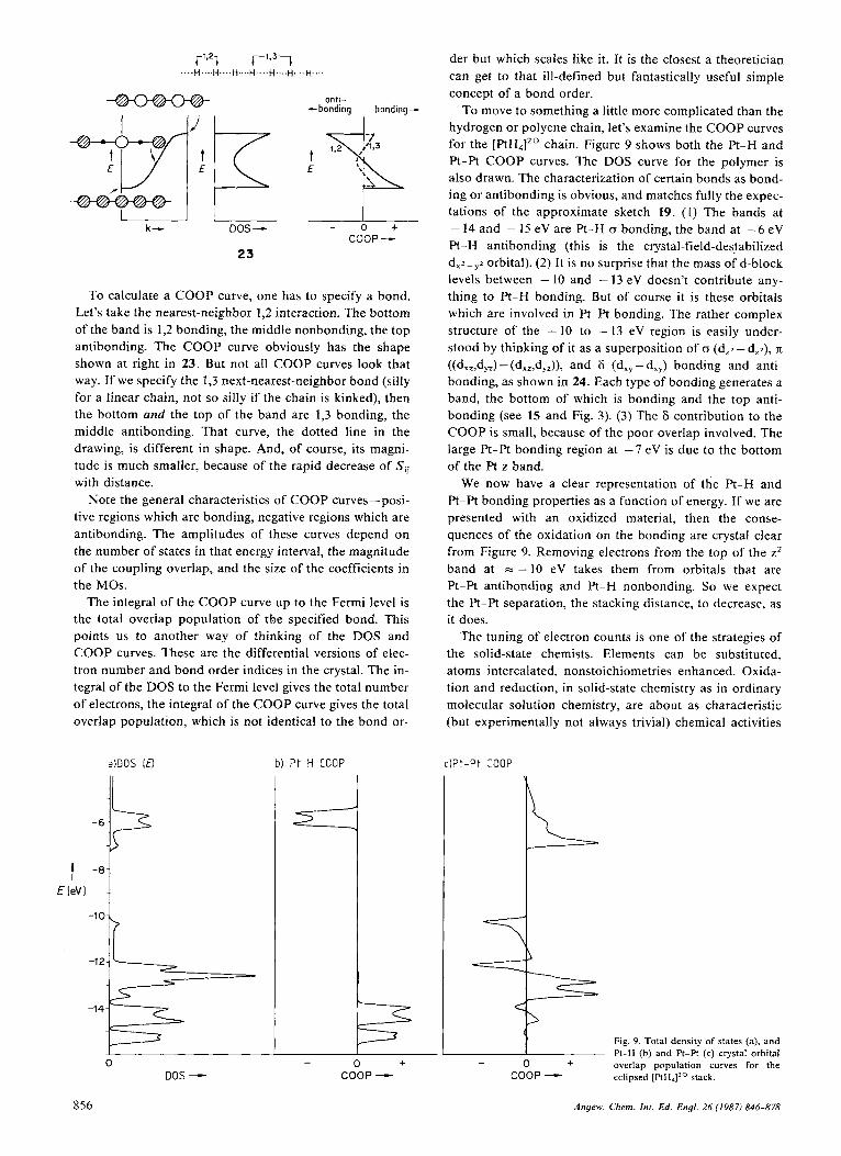
To move to something a little more complicated than the hydrogen or polyene chain, let’s examine the COOP curves for the [RH,]” chain. Figure 9 shows both the R-H and R-Pt COOP curves. The DOS curve for the polymer is also drawn. The characterization of certain bonds as bonding or antibonding is obvious, and matches fully the expectations of the approximate sketch 19. (1) The bands at - 14 and - 15 eV are R-H cs bonding, the band at -6 eV R-H antibonding (this is the crystal-field-destabilized dX2-yZ orbital). (2) It is no surprise that the mass of d-block levels between - 10 and - 13 eV doesn’t contribute anything to Pt-H bonding. But of course it is these orbitals which are involved in R-Pt bonding. The rather complex structure of the - 10 to - 13 eV region is easily understood by thinking of it as a superposition of CT ( d , ~ - dZ2), n ((dxz,dyz) - (dxz,dyz)), and 6 (dxy - dxy) bonding and antibonding, as shown in 24. Each type of bonding generates a band, the bottom of which is bonding and the top antibonding (see 15 and Fig. 3) . ( 3 ) The 6 contribution to the COOP is small, because of the poor overlap involved. The large R-Pt bonding region at -7 eV is due to the bottom of the Pt z band.

We now have a clear representation of the R-H and Pt-Pt bonding properties as a function of energy. If we are presented with an oxidized material, then the consequences of the oxidation on the bonding are crystal clear from Figure 9. Removing electrons from the top of the zz band at = - 10 eV takes them from orbitals that are R-Pt antibonding and R-H nonbonding. So we expect the Pt-Pt separation, the stacking distance, to decrease, as it does.

The tuning of electron counts is one of the strategies of the solid-state chemists. Elements can be substituted, atoms intercalated, nonstoichiometries enhanced. Oxida- tion and reduction, in solid-state chemistry as in ordinary molecular solution chemistry, are about as characteristic (but experimentally not always trivial) chemical activities

C P - P t COOP

Fig. 9. Total density of states (a), and R-H (b) and pt-pt (c) crystal orbital overlap population curves for the eclipsed [PtH4]20 stack.

0 COOP -

856 Angew. Chem. ln l . Ed. Engl. 26 (1987) 846-878

I , - - o + - o +

-20 -

-25 -

-30 -,

c-2 COOP - ?r-xz,yz COOP - - o + - o +

8 - x y COOP - totalCOOP -

as one can conceive. The conclusions we reached for the pt-Pt chain were simple, easily anticipated. Other cases are guaranteed to be more complicated. The COOP curves allow one, at a glance, to reach conclusions about the local effects on bond length (will bonds be weaker, stronger) upon oxidation or reduction.

We showed earlier a band structure for rutile (Fig. 5b, repeated in Fig. 10a). The corresponding COOP curve for the Ti-0 bond (Fig. lob) is extremely simple. Note the bonding in the lower, oxygen bands, and antibonding in the eg crystal-field-destabilized orbital. The tZp is, as expected, Ti-0 “n-antibonding.”

Let’s try our hand at predicting the DOS for something quite different from [PtH,IZQ or Ti02, namely, a bulk transition metal, the face-centered cubic Ni structure. Each metal atom has as its valence orbitals 3d, 4s, and 4p, or- dered in energy approximately as at the left in 25. Each will spread out into a band. We can make some judgment as to the width of the bands from the overlap. The s,p orbitals are diffuse, their overlap will be large, and a wide band will result. They also mix with each other extensively. The d orbitals are contracted, and so will give rise to a relatively narrow band.

The computed DOS for bulk Ni (bypassing the actual band structure) is shown in Figure 1 1 , along with the Ni s and p contributions to that DOS. What is not s or p is d.

-5 ‘B t -lo B-

-35 L 00s -

The general features of 25 are reproduced. At the Fermi level, a substantial part of the s band is occupied, so that the c a l c ~ l a t e d ~ ” ~ Ni configuration is d9 ‘ss0.62p0.23.

1

DOS - What would one expect of the COOP curve for bulk Ni?

As a first approximation we could generate the COOP curve for each band separately (26a, b). Each band in 25 has a lower Ni-Ni bonding part, an upper Ni-Ni antibonding part. The composite is 26c. The computed COOP curve is in Figure 12. The expectations of 26c are met rea- sonably well.

A metal-metal COOP curve like that of 26c or Figure 12 is expected for any transition metal. The energy levels

4

L antibonding - 0 + bonding

COOP - Fig. 10. a) DOS and b) Ti-0 COOP for rutile.

857 Angew. Chem. lnt. Ed. Engl. 26 11987) 846-878

a ) I [ % I - b) I [ % I - 0 100 0 100

10 I I "

a b C

5

0

-5

-10

-15 . ' - 1 5 ' . ' . ' . ' 00s - 00s -

Fig. I I . Iota1 I)OS (dashed line) and 4, (a) and 4p (h) contrihutionr to it in bulk Ni. The dotted line is an integration of the occupation of a specified orbital, on a scale of 0 to 100% given at top.

might be shifted up, they might be shifted down, but their bonding characteristics are likely to be the same. If we assume that a similar band structure and COOP curve hold for all metals (in the solid-state trade this would be called the rigid band model), then Figure 12 gains tremendous power. It summarizes, simply, the cohesive energies of all metals. As one moves across the transition series, the M-M overlap population (which is clearly related to the binding or cohesive energy) will increase, peaking at about six electrons per metal (Cr, Mo, W). Then it will decrease toward the end of the transition series and rise again for small s,p electron counts. For more than I4 electrons, a metal is unlikely; the net overlap population for such high coordination becomes negative. Molecular allotropes with lower coordination are favored. There is much more to cohesive energies and the metal-nonmetal transition than this, but

a1

lo 1

- o + - o + - 0 + d COOP- s , p COOP- total COOP-

there is much physics and chemistry that flows from the simple construction of 26.

With a little effort, we have constructed the tools-density of states, its decompositions, the crystal orbital overlap population-which allow us to move from a complicated, completely delocalized set of crystal orbitals or Bloch functions to the localized, chemical description. There is no mystery in this motion. In fact, what I hope I have shown here is just how much power there is in the chemists' concepts. The construction of the approximate DOS and bonding characteristics of a [(PtH,)"], polymer, or rutile, or bulk Ni, is really easy.

Of course, there is much more to solid-state physics than band structures. The mechanism of conductivity, the remarkable phenomenon of superconductivity, the multitude of electric and magnetic phenomena that are special to the solid state, for these one needs the tools and ingenuity of physics.[61 But as for bonding in the solid state, I think (some will disagree) there is nothing new, only a different language.

More Than One Electronic Unit in the Unit Cell: Folding Bands

The oxidized cyanoplatinates are not eclipsed (27a), but staggered (27b). A polyene is not a simple linear chain, 28a, but, of course, at least s-trans or zigzag, 28b. Or it could be s-cis, 28c. And obviously that does not exhaust the possibility of arrangements. Nature always seems to

27

28 b

~ 1 5 J I 00s - antibonding - 0 +bonding

COOP - Fig. 12. a) The total DOS and h) nearest-neighbor N t - N i COOP in bulk Ni.

find one we haven't thought of. In 27a and 28a, the unit cell contains one basic electronic unit, [F'tH,]2e and a CH group, respectively. In 27b and 28b, the unit is doubled, approximately so in unit cell dimension, exactly so in

858 Angew. Chem. Int. Ed Engl 26 (1987) 846-878

chemical composition. In 28c, we have four C H units per unit cell. A purely physical approach might say each is a case unto itself. A chemist is likely to say that probably not much has changed on doubling or quadrupling or mul- tiplying by 17 the contents of a unit cell. If the geometrical distortions of the basic electronic unit that is being repeated are not large, it is likely that any electronic characteristics of that unit are preserved.

The number of bands in a band structure is equal to the number of molecular orbitals in the unit cell. So if the unit cell contains 17 times as many atoms as the basic unit, it will contain 17 times as many bands. The band structure may look messy. The chemist’s feeling that the “17-mer” is a small perturbation on the basic electronic unit can be used to simplify a complex calculation. Let’s see how this goes, first for the polyene chain, then for the [(PtH4JZQ], polymer.

28a, b, and c differ from each other not just in the number of C H entities in the unit cell, but also in their geometry. Let’s take these one at a time. First prepare for the distortion from 28a to 28b by doubling the unit cell, and then, subsequently, distorting. This sequence of actions is indicated in 29.

-0- . . . , . . . 0

.-20-: :

29 b

C

but they obviously have the same nodal structure-one node every two centers.

If we now detach ourselves from this viewpoint and go back and construct the orbitals of the one C H per unit cell linear chain 29a, we get 32. The Brillouin zone in 29b is half as long as it is here, because the unit cell is twice as long.

32

-a

At this point, the realization hits us that, of course, the orbitals of these polymers are the same. The polymers are identical, it is only some peculiar quirk that made us choose one C H unit as the unit cell in one case, two C H units in the other. I have presented the two constructions independently to make explicit the identity of the orbitals.

What we have is two ways of presenting the same orbitals. Band structure 31, with two bands, is identical to 32, with one band. All that has happened is that the band of the minimal polymer, one C H per unit cell, has been “folded back” in 32. The process is shown in 33.“’’

Suppose we construct the orbitals of 29b, the doubled unit cell polymer, by the standard prescription: ( I ) get MOs in unit cell, (2) form Bloch functions from them. Within the unit cell the MOs of the dimer are n and n*. 30.

- l 7

CZHB -lT

30

Each of these spreads out into a band, that of the n “running up,” that of n* “running down,” 31. The orbitals are written out explicitly at the zone boundaries in 31. This

31

allows one to see that the top of the n band and the bottom of the x* band, both at k = n /2a , are precisely degenerate. There is no bond alternation in this polyene (yet), and the two orbitals may have been constructed in a different way,

n ‘= 20

33

The process can be continued. If the unit cell is tripled, the band will fold as in Ma. If it is quadrupled, we get 34b, and so on. However, the point of all this is not just

a ’ = 30 a ‘ = 40

0 b 34

redundancy, seeing the same thing in different ways. There are two important consequences or utilizations of this folding. First, if a unit cell contains more than one electronic unit (and this happens often), then a realization of that fact, and the attendant multiplication of bands (remember

Angew. Chem. Int. Ed. Engl. 26 11987) 846-878 859

32- 31, 34a, or 34b), allows a chemist to simplify in his or her mind the analysis. The multiplicity of bands is a consequence of an enlargement of the unit cell. By reversing, in our minds in a model calculation, the folding process, by unfolding, we can go back to the most fundamental electronic act-the true monomer.

-1 5 L .- 0 k- R/0' 0 k - - c n/a'

Fig. 13. The band structure of a staggered [PtH41-'O stack (a), compared with the folded-back band structure of an eclipsed stack, two [PtH,]'' in a unit cell (b).

To illustrate this point, let me show the band structure of the staggered [PtH4]*0 chain, 27b. This is done in Figure 13a. There are twice as many bands in this region as there are in the case of the eclipsed monomer (the xy band is doubly degenerate). This is no surprise; the unit cell in the staggered polymer is [(PtH4)ZQ]2. But it's possible to understand Figure 13 as a small perturbation on the eclipsed polymer. Imagine the thought process 35a -+ 35b- 3512, i.e., doubling the unit cell in an eclipsed polymer and then ro- tating every other unit by 45" around the z axis. To go

from 35a to 35b is trivial, a simple folding back. The result is shown in Figure 13b. Figures 13a and 13b are nearly identical. There is a small difference in the xy band, which is doubled, nondegenerate, in the folded-back eclipsed po-

lymer (Fig. 13b), but degenerate in the staggered polymer. What happened here could be stated in two ways, both the consequence of the fact that a real rotation intervenes between 35b and 35c. From a group-theoretical point of view, the staggered polymer has a new, higher symmetry element, an eightfold rotation-reflection axis. Higher symmetry means more degeneracies. It is easy to see that the two combinations, 36, are degenerate.

Except for this minor wrinkle, the band structures of the folded-back eclipsed polymer and the staggered one are very, very similar. That allows us to reverse the argument, to understand the staggered one in terms of the eclipsed one plus the here minor perturbation of rotation of every second unit.

The chemist's intuition is that the eclipsed and staggered polymers can't be very different. At least until the ligands start bumping into each other, and for such steric effects there is, in turn, much further intuition. The band structures may look different, for one polymer has one, the other two basic electronic units in the cell. Chemically, however, they should be similar, and we can see this by returning from reciprocal space to real space. Figure 14, comparing the DOS of the staggered (Fig. 14a) and eclipsed (Fig. 14b) polymers, shows just how alike they are in their distribution of levels in energy.

a) staggered b) eclipsed

E LeVl ' b

DOS - DOS - Fig. 14. A comparison of the 110s of staggered ( d ) m d rcl~psed (b) 1PtH,jZQ stacks.

There is another reason for feeling at home with the folding process. The folding-back construction may be a prerequisite to understanding a chemically significant distortion of the polymer. To illustrate this point, we return to the polyene 29. To go from 29a to 29b involves no distortion. However, 29b i s a way point, a preparation for a real distortion to the more realistic "kinked" chain, 29c. It be- hooves us to analyze the process stepwise if we are to understand the levels of 29c.

Of course, nothing much happens to the n system of the polymer on going from 29a,b to 29c. If the nearest-neighbor distances are kept constant, then the first real change is

860 Angew. Chem. In!. Ed. Engl. 26 11987) 846-878

in the 1,3 interactions. These are unlikely to be large in a polyene, since the x overlap falls off very quickly past the bonding region. We can estimate what will happen by writing down some explicit points in the band, and deciding whether the 1,3 interaction that is turned on is stabilizing or destabilizing. This is done in 37. Of course, in a real CH

stabilized

37 destabilized

stabilized

polymer this kinking distortion is very much a real thing, but that has nothing to d o with the n system, it’s a result of strain.

However, there is another distortion which the polyene can and does undergo. This is double-bond localization, an example of the very important Peierls distortion, the solid-state analogue of the Jahn-Teller effect.

Making Bonds in a Crystal

When a chemist sees a molecular structure which contains several free radicals, orbitals with unpaired electrons, his inclination is to predict that such a structure will undergo a geometry change in which electrons will pair up, forming bonds. It is this reasoning, so obvious as to seem almost subconscious, which is behind the chemist’s intuition that a chain of hydrogen atoms will collapse into a chain of hydrogen molecules.

If we translate that intuition into a molecular orbital picture, we have 38a, a bunch (here six) of radicals forming bonds. That process of bond formation follows the Hz paradigm, 38b, i.e., in the process of making each bond a level goes down, a level goes up, and two electrons are stabilized by occupying the lower, bonding orbital.

In solid-state physics, bond formation has not stood at center stage, as it has in chemistry. The reasons for this are obvious: the most interesting developments in solid-state physics have been around metals and alloys, and in these

often close-packed or nearly close-packed substances, by and large localized chemical viewpoints have seemed irrel- evant. For another large group of materials, ionic solids, it also seemed useless to think of bonds. My contention is that there is a range of bonding, including what are usually called metallic, covalent, and ionic solids, and that there is, in fact, substantial overlap between seemingly divergent frameworks of describing the bonding in these three types of crystals. I will take the view that the covalent approach is central and look for bonds when others wouldn’t think they’re there. One reason for tolerating such foolhardiness might be that the other approaches (metallic, ionic) have had their day-why not give this one a chance? A second reason, one I’ve mentioned earlier, is that, in thinking and talking about bonds in the crystal, one makes a psycholog- ically valuable connection to molecular chemistry.

To return to our discussion of molecular and solid-state bond formation, let’s pursue the trivial chemical perspective of the beginning of this section. The guiding principle, implicit in 38, is: Maximize bonding. There may be impedi- ments to bonding: electron repulsions, steric effects, i.e., the impossibility of two radicals to reach within bonding distance of each other. Obviously, the stable state is a com- promise-some bonding may have to be weakened to strengthen some other bonding. But, in general, a system will distort so as to make bonds out of radical sites. Or to translate this into the language of densities of states: max- imizing bonding in the solid state is connected to lowering the DOS at the Ferrni level, moving bonding states to lower energy, antibonding ones to high energy.

The Peierls Distortion

In considerations of the solid state, a natural starting point is high symmetry-a linear chain, a cubic or close- packed three-dimensional lattice. The orbitals of the highly symmetrical, idealized structures are easy to obtain, but tbey often d o not correspond to situations of maximum bonding. These are less symmetrical, deformations of the simplest, archetype structure.

The chemist’s experience is usually the reverse, beginning from localized structures. However, there is one piece of experience we have that matches the way of thinking of the solid-state physicist. This is the Jahn-Teller effect,”91 and it’s worthwhile to show its working by a simple example.

The Huckel R MOs of a square-planar cyclobutadiene are well known. They are the one-below-two-below-one set shown in 39. a -

q4

We have a typical Jahn-Teller situation-two electrons in two degenerate orbitals. (Of course, we need worry

Angen’. Chem. In( . Ed. Engl. 26 (1987) 846-878 86 1

about the various states that arise from this occupation, and the Jahn-Teller theorem really applies to only one.”91) The Jahn-Teller theorem says that such a situation necessi- tates a large interaction of vibrational and electronic motion. It states that there must be at least one normal mode of vibration which will break the degeneracy and lower the energy of the system (and, of course, lower its symmetry). It even specifies which vibrations would accomplish this.

In the case at hand the most effective normal mode is illustrated in 40. It lowers the symmetry from D4,, to DZhr and, to use chemical language, localizes double bonds.

40

The orbital workings of this Jahn-Teller distortion are easy to see. 41 illustrates how the degeneracy of the e orbital is broken in the two phases of the vibration. On forming the rectangle as at right in 40 or 41, ryz is stabilized:

41

the 1-2 and 3-4 interactions, which were bonding in the square, are increased; the 1-4 and 2-3 interactions, which were antibonding, are decreased by the deformation. The reverse is true for ry3-it is destabilized by the distortion at right. If we follow the opposite phase of the vibration (to the left in 40 or 41), ry, is stabilized, ry2 destabilized.

The essence of the Jahn-Teller theorem is revealed here: a symmetry-lowering deformation breaks an orbital degeneracy, stabilizing one orbital, destabilizing another. Note the phenomenological correspondence to 38 in the previous section.

One doesn’t need a real degeneracy to benefit from this effect. Consider a nondegenerate two-level system, 42,

42 - A - C

+ 8 - C

with the two levels of different symmetry (here labeled A and B) in one geometry. If a vibration lowers the symmetry so that these two levels transform as the same irreducible representation (call it C), then they will interact, mix, repel each other. For two electrons, the system will be stabilized. The technical name of this effect is a second-order Jahn- Teller def~rmation.~”]

The essence of the Jahn-Teller effect, first or second order, is : a high-symmetry geometry generates a degeneracy or near degeneracy, which can be broken, with stabilization, by a symmetry-lowering deformation. Note a further point: the level ,degeneracy is not enough by itself-one needs the right electron count. The cyclobutadiene (or any square) situation of 39 will be stabilized by a DzI, deformation for three, four, or five electrons, but not for two or six (e.g., s:@).

This framework we can take over to the solid. There is degeneracy and near degeneracy for any partially filled band. The degeneracy is that already mentioned, for E(k) = E( - k) for any k in the zone. The near degeneracy is, of course, for k’s just above or just below the specified Fermi level. For any such partially filled band there is, in principle, available a deformation which will lower the energy of the system. In the jargon of the trade one says that the partial filling leads to an electron-phonon coupling which opens up a gap just at the Fermi level. This is the Peierls distortion,f201 the solid-state counterpart of the Jahn-Teller effect.

Let’s see how this works on a chain of hydrogen atoms (or a polyene). The original chain has one orbital per unit cell, 43a, and an associated simple band. We prepare it for

-:I / kEF a W I

deformation by doubling the unit cell, 43b. The band is typically folded. The Fermi level is halfway up the band- the band has room for two electrons per orbital, but for H or CH we have one electron per orbital.

44

The phonon or lattice vibration mode that couples most effectively with the electronic motions is the symmetric pairing vibration, 44. Let’s examine what it does to typical orbitals at the bottom, middle (Fermi level), and top of the band, 45.

-Y I . o k- r112ni


At the bottom and top of the band nothing happens. What is gained (lost) in increased 1-2, 3-4, 5-6, etc. bonding (antibonding) is lost (gained) in decreased 2-3, 4-5, 6- 7, etc. bonding (antibonding). But in the middle of the band, at the Fermi level, the effects are dramatic. One of the degenerate levels there is stabilized by the distortion, the other destabilized. Note the phenomenological similar- ity to what happened for cyclobutadiene.

The action does not take place just at the Fermi level, but in a second-order way the stabilization “penetrates” into the zone. It does fall off with k, a consequence of the way perturbation theory works. A schematic representation of what happens is shown in 46 ( I and I 1 represent the

I = - - * - = t t

11 -

chain before and after the distortion). A net stabilization of the system occurs for any Fermi level, but obviously it is maximal for the half-filled band, and it is a t the E~ that the band gap is opened up. If we were to summarize what happens in block form, we’d get 47. Note the resemblance to 38.

i:

The polyene case (today it would be called polyacetylene) is especially interesting, for some years ago it occa- sioned a great deal of discussion. Would an infinite polyene localize (48)? Eventually, Salem and Longuet-Hig-

m. 0 - 48

gins demonstrated that it would.“” Polyacetylenes are an exciting field of modern Pure polyacetylene is not a conductor. When it is doped, either partially filling the upper band in 45 or emptying the lower, it becomes a superb conductor.

There are many beautiful intricacies of the first- and second-order and low- or high-spin Peierls distortion, and for these the reader is referred to the very accessible review by

The Peierls distortion plays a crucial role in determining the structure of solids in general; the one-dimensional pairing distortion is only one simple example of its workings. Let’s move up in dimensionality.

Whangbo. f51

One ubiquitous ternary structure is that of PbFCl (ZrSiS, BiOCI, Co,Sb, FezAs).123.241 We’ll call it MAB here, because in the phases of interest to us the first element is often a transition metal, the other components, A, 9, often main-group elements. 49 shows one view of this structure, 50 another.

9 49 50

In this structure we see two associated square nets of M and B atoms, separated by a square-net layer of A’s. The A layer is twice as dense as the others, hence the MAB stoichiometry. Most interesting, from a Zintl viewpoint, is a consequence of that A layer density, a short A-A contact, typically 2.5 A for Si. This is definitely in the range of some bonding. There are no short 9 - B contacts.

Some compounds in this series in fact retain this structure. Others distort. It is easy to see why. Take GdPS. If we assign normal oxidation states of Gd3@ and S ’ O , we come to a formal charge of P” on the dense-packed P net. From a Zintl viewpoint, Po is like S and so should form two bonds per P. This is exactly what it does. The GdPS struc-

U

51

Angew. Chem. In,. Ed. Engl. 26 11987) 846-878 863

t ~ r e [ * ~ ] is shown in 51, which is drawn after the beautiful representation of HuNiger et al.'"] Note the P-P cis chains in this elegant structure.

From the point of view of a band structure calculation one might also expect bond formation, a distortion of the square net. 52 shows a qualitative DOS diagram for GdPS.

t E

I

I) Gd d

h P 3P

s 3 P

52

What goes into the construction of this diagram is a judgment as to the electronegativities ( G d < P<S). And the structural information that there are short P-P interactions in the undistorted square net, but no short S-S contacts. With the normal oxidation states of Gdse and SZQ one comes to Pe, as stated above. This means the P 3p band is 2/3 filled. The Fermi level is expected to fall in a region of a large DOS, as 52 shows. A distortion should follow.

The details of what actually happens are presented elsewhere.'241 The situation is intricate; the observed structure is only one likely way for the parent structure to stabilize- there are others. 53 shows some possibilities suggested by HulIiger et a1.[251 CeAsS chooses 5 3 ~ . ~ * ~ ] Nor is the range of geometrical possibilities of the MAB phases exhausted by these. Other deformations are possible; many of them can be rationalized in terms of second-order Peierls distortions in the

An interesting three-dimensional instance of a Peierls distortion at work (from one point of view) is the derivation of the observed structures of elemental arsenic and black phosphorus from a cubic lattice. This treatment is due to Burdett and c o - w o r k e r ~ . ~ ~ ~ ~ ~ ' The two structures are shown in their usual representation in 54. It turns out that they can be easily related to a simple cubic structure, 55.

The DOS associated with the band structure of 55, with one element of the fifth main group per lattice site must

0 0 0 0

54 55

have the block form 56. There are five electrons per atom, so if the s band is completely filled, we have a half-filled p band. The detailed DOS is given elsewhere.[271 What is significant here is what we see without calculations, namely, a half-filled band. This system is a good candidate for a Peierls distortion. One pairing up of all the atoms along the x, y, and z directions will provide the maximum stabilization, indicated schematically in 57.

ns

DOS -

P

56 57

Burdett, McLarnan, and Haaland~'7".cJ have shown that there are no less than 36 different ways to so distort. Two of these correspond to black phosphorus and arsenic, 58. There are other possibilities.

There is one aspect of the outcome of a Peierls distortion, the creation of a gap at the Fermi level, that might be taken from the last case as being typical, but which is not necessarily so. In one dimension one can always find a Peierls distortion to create a gap. In three dimensions, atoms are much more tightly linked together. In some cases a stabilizing deformation leads to the formation of a real band gap, to an insulator or semiconductor. In other cases, a deformation is effective in producing bonds, pull-

864 Angew. Chem. In[. Ed. Engl. 26 (1987) 846-878

60

ing some states down from the Fermi level region. But because of the three-dimensional linkage it may not be possible to remove all the states from the Fermi level region. Some DOS remains there; the material may still be a conductor.

The applications discussed in this section make it clear that one must know, at least approximately, the band structure (and the consequent DOS) of two- and three- dimensional materials before one can make sense of their marvelous geometrical richness. The band structures that we have discussed in detail have been one-dimensional. Now let’s look more carefully a t what happens as we increase dimensionality.

More Dimensions

Most materials are two- or three-dimensional, and while one dimension is fun, we must eventually leave it for higher dimensionality. Nothing much new happens, except that we must treat as a vector, with components in reciprocal space, and the Brillouin zone is now a two- or three- dimensional area or volume.[6. ‘’]

To introduce some of these ideas, let’s begin with a square lattice, 59, defined by the translation vectors 5, and

a,. Suppose there is a n H 1s orbital on each lattice site. It turns out that the Schrodinger equation in the crystal factors into separate wave equations along the x and y axes, each of them identical to the one-dimensional equation for a linear chain. There is a k, and a k,, the range of each is 0 I IkJ, Ik,l5 n/a (a = IG,] = I&/). Some typical solutions are shown in 60.

The construction of these is obvious. What the construction also shows, very clearly, is the vector nature of k. Con- sider the (kx, kY)=(n/2a, d 2 n ) and (rr/a,n/a) solutions. A look at them reveals that they are waves running along a direction which is the vector sum of k, and k,, i.e., on a diagonal. The wavelength is inversely proportional to the magnitude of that vector.

The space of k here is defined by two vectors 6! and 6;, and the range of allowed k, the Brillouin zone, is a square.

k,= r / a , k y = O

X

r k,=O, k ,=O

k,. k, = r / ( Z a )

k , , ky = r / a

M

k, = 0, k y = r / (Za l

k , = O , k y = r / a

X

Certain special values of k are given names: r=(O,O) is the zone center, X = ( d a , 0) = (0, d a ) , M = ( d a , d a ) . These are shown in 61, and the specific solutions for r, X, M were so labeled in 60.

It is difficult to show the energy levels, E ( l ) for all k: So what one typically does is to illustrate the evolution of E along certain lines in the Brillouin zone. Some obvious ones are T-+X, r + M , X-M. From 60 it is clear that M is the highest energy wave function, and that X is pretty much nonbonding, since it has as many bonding interactions (along y) as it does antibonding ones (along x). So we would expect the band structure to look like 62. A computed band structure and DOS for a hydrogen lattice with a=2.0 A (Fig. 15) confirms our expectations.

62 1 E

r x M r k -

The chemist would expect the chessboard of H atoms to distort into one of H2 molecules (an interesting problem is how many different ways there are to accomplish this). The large peak in the DOS for the half-filled H square- lattice band would make the physicist think of a lattice vibration that would create a gap at E ~ . Any pairwise deformation will d o that.

Angew. Chem. Int. Ed. Engl. 26 (1987) 846-878 865

r 00s - -20- ~ X M

Fig. 15. a) The band.structure and b) DOS of a square lattice of H atoms; H-H separation 2.0 A.

Let's now put some p orbitals on the square lattice, with the direction perpendicular to the lattice taken as z. The pz orbitals will be separated from pr and px by their symmetry. Reflection in the plane of the lattice remains a good symmetry operation at all k. The pz(z) orbitals will give a band structure similar to that of the s orbitals, for the topology of the interaction of these orbitals is similar. This is why in the one-dimensional case we could talk at one and the same time about chains of H atoms and polyenes.

The px and pr orbitals present a somewhat different problem. Shown in 63 are the symmetry-adapted combinations of each at r, X, Y, and M. (Y is by symmetry equiva-

ff,7r*

r

X

63

Y

M ff, 7r*

1

lent to X ; the difference is just in the propagation along x or y.) Each crystal orbital can be characterized by the p, p CJ or n bonding present. Thus at the x and y combinations are CJ antibonding and n bonding; at X they are o and n bonding (one of them), and and n antibonding (the other). At M they are both CJ bonding, n antibonding. It is also clear that the x,y combinations are degenerate at r and M (and it turns out along the line r-+ M, but for that one needs a little group and nondegenerate at X and Y (and everywhere else in the Brillouin zone).

Putting in the estimate that o bonding is more important than n bonding, one can order these special symmetry points of the Brillouin zone in energy, and draw a qualitative band structure (Fig. 16). The actual appearance of any

p+ r x k x

r X M r k-

Fig. 16. Schematic band structure of a planar square lattice of atoms bearing ns and rip orbitals. The s and p levels have a large enough separation that the s and p bands do not overlap.

real band structure (e.g., the P net in GdPS discussed in the last section) will depend on the lattice spacing. Band dis- persions will increase with short contacts, and complications due to s,p mixing will arise. Roughly, however, any square lattice, be it the P net in GdPS,'241 a square over- layer of S atoms adsorbed on Ni(100),[28"1 the oxygen and lead nets in litharge,'28b1 a Si layer in BaPdSij,[Zxcl will have these orbitals.

Three dimensions really introduce little new, except for the complexities of drawing and the wonders of group theory in the 230 space groups. The s, p, and d bands of a cubic lattice, or of face-centered or body-centered close- packed structures, are particularly easy to construct.

Let's look at a three-dimensional case of some complexity, the NiAs- MnP- NIP distortion.[291 First, the chemical


. V 0 s

motivation. The NiAs structure is one of the most common AB structures, with over a hundred well-characterized materials crystallizing in this type. The structure, shown in three different ways in 64, consists of hexagonal close- packed layers which alternate metal and non-metal atoms. To be specific, let’s discuss the VS representative. The structure contains a hexagonal layer of vanadium atoms at z = 0, then a layer of sulfur atoms at z= 1/4, then a second layer of metal atoms at z= 112, superimposable on the one at z = 0, and, finally, a second layer of main group atoms at z=3/4. The pattern is repeated along the c direction to generate a three-dimensional stacking of the type aBaCa- BaC. I t should not be imagined, however, that this is a layered compound; it is a tightly connected three-dimensional array. The axial V-V separation is 2.94 A; the V-V contacts within the hexagonal net are longer (3.33

In terms of local coordination, each sulfur sits a t the center of a trigonal prism of vanadiums, which in turn are octahedrally coordinated by six sulfurs. The V-S distances are typical of coordination compounds and, while there is no S-S bonding, the sulfurs are in contact with each other.

This is the structure of stoichiometric VS at high temper- atures (> 550°C). At room temperature, the structure is a lower symmetry, an orthorhombic MnP one. The same structural transition is triggered by a subtle change in stoichiometry in VS,, by lowering x from 1 a t room tempera- t u re.[”’]

The MnP structure is a small but significant perturbation on the NiAs type. Most (but not all) of the motion

a) vanadium sulfide (NiAs structure) b) sulfur sublattice in VS

64

0 v at z=0.0 0 V at 2.0.5 0 S at 2.0.25 @a S at z = 0.75

takes place in the plane perpendicular to the hexagonal axis. The net effect in each hexagonal net is to break it up into zigzag chains, as in 65. The isolation of the chains is

exaggerated: the short V-V contact emphasized in 65 changes from 3.33 A to 2.76 A, but the V-V distance perpendicular to the plane (not indicated in 65) is not much longer (2.94 A).

Still further distortions can take place. In NIP, the chains of Ni and P atoms discernible in the MnP structure break up into Ni, and P2 pairs. For phosphides, it is experimentally clear that the number of available electrons tunes the transition from one structural type to another. Nine or ten valence electrons favor the NiAs structure (for phosphides), 11 to 14 the MnP, and a greater number of electrons prefers the NIP alternative. For the arsenides this trend is less clear.

The details of these fascinating transformations are given elsewhere.f2Y1 It is clear that any discussion must begin with the band structure of the “aristotype,” NiAs (here computed for VS). This is presented in Figure 17.

A veritable spaghetti diagram this, seemingly beyond the powers of comprehension of any human being. Why not abdicate understanding, just let the computer spew these bands out and accept (or distrust) them? No, that’s too

-15

r M K M K r n

c ) vanadium sublattice in VS

k- k- k-

Angew. Chem. In l . Ed. Engl. 26 (1987) 846-878

Fig. 17. The band structure for VS in the NiAs structure (a), together with the band structures of its S (b) and V (c) sublattices.

867

easy a way out. We can understand much of this dia-

First, the general aspects. The hexagonal unit cell is shown in 66. It contains two formula units V2Sz. That tells us immediately that we should expect 4 x 2 = 8 sulfur bands, two 3s separated from six 3p. And 9 x 2 = 18 vanadium bands, of which 10, the 3d block, should be lowest.

gram.

Ak3

66 67

The Brillouin zone (67) has some special points labeled in it. There are conventions for this labeling.[6,'51 The zone is, of course, three-dimensional. The band structure (Fig. 17) shows the evolution of the levels along several directions in the zone. Count the levels in Figure 17a to confirm the presence of six low-lying bands (which a decomposition of the DOS shows to be mainly S 3p) and ten V 3d bands. The two S 3s bands are below the energy window of the drawing. At some special points in the Brillouin zone there are degeneracies, so one should pick a general point to count bands.

A feeling that this structure is made up of simpler components can be pursued by decomposing it into V and S sublattices (Fig. 17b,c). Note the relatively narrow V d bands around - 8 to - 9 eV. There is metal-metal bonding in the V sublattice; the widths of the V s,p bands show this. There are also changes in the V d bands on entering the composite VS lattice. A chemist would look for the local t2g-e, splitting, characteristic of vanadium's octahedral environment.

Each of these component band structures could be understood in further Take the S 3p substructure at r. The unit cell contains two S atoms, redrawn in a two-

68 x \ dimensional slice of the lattice in 68 to emphasize the in- version symmetry. 69-71 are representative x,y and z com-

69 70 71

binations of one S two-dimensional hexagonal layer at r. Obviously, x and y are degenerate, and the x,y combination should be above z-the former is locally a antibonding, the latter n bonding. Now combine two layers. The x,y layer Bloch functions will interact less (x overlap) than the z functions (a antibonding for the r point, 72). These

qualitative considerations (x,y above z, the z bands split more than the x,y bands) are clearly visible in the position- ing of the S 3p bands in Figures 17b and 17a.

With more, admittedly tedious, work, every aspect of these spaghetti diagrams can be understood. And, much more interestingly, so can the electronic tuning of the NiAs- MnP- NIP displacive transition.'291

A Sample Problem: The ThCr,Si, Structure

The preceding sections have outlined some of the theoretical tools for analysis of bonding in the solid state. To see how these ideas can be integrated, let's discuss a specific problem.

More than 400 compounds of AB2X2 stoichiometry adopt the ThCr2Si2 type structure,[3z1 but you are not likely to find any mention of these in any modern textbook of general inorganic chemistry, which just tells us something about the ascendancy of molecular inorganic chemistry, especially transition-metal organometallic chemistry, in the last three decades. However, these compounds are there, we know their structures and they have interesting properties. A is typically a rare-earth, alkaline-earth, or al- kali element, B is a transition metal or main-group element, and X comes from the fifth, fourth, and occasionally third main group. Since the synthesis of ABzX2 with A = a rare-earth element, by Parthh, Rossi, and their co-workers, the unusual physical properties exhibited by these solids have attracted much attention. Physicists speak with en- thusiasm of valence fluctuation, p-wave or heavy-fermion superconductivity and of many peculiar magnetic properties of these materials. The very structure of these materials carries much that is of interest to the chemist.

The ThCr2Si2 structure type for AB2X2 stoichiometry compounds is shown in 73. It consists of BzX2 layers inter- spersed with A layers. The bonding between A and B2X2 layers appears largely ionic, which is why we may write the charge partitioning as A'@ and B,X$". But in the B2Xz layer there is indication not only of covalent B-X bonding, but also some metal-metal B-B bonding. Typical metal- metal distances are in the range of 2.7-2.9 A.

A way to describe the B2Xz layers in these compounds is to imagine a perfect square-planar two-dimensional lattice of metal atoms B, above and below the fourfold hollows of which lie the main-group X atoms. This is shown in 74.

73 O X 0 5

74

868 Angew. Chem Int. Ed. Engl. 26 (1987) 846-878

The coordination environment of the metal atom B is approximately tetrahedral in the main-group elements X, with four additional square-planar near-neighbor metal atoms B. The coordination of the X atoms is much more unusual-they reside at the apex of a square pyramid.

It may be noted here that there are alternative ways to describe the layer structure. For instance, the B2X2 layer may be thought of as being built up by sharing four of the six edges of a BX, tetrahedron by infinite extension in two dimensions, as in 75. Such packing diagrams, or alterna-

X-fX

x---X -

7 5

tive ways of looking at the same structure, are inherently useful-a new view often leads to new insight. I would just introduce a very personal prejudice, voiced above, for views of structure that make as many connections as possible to other subfields of chemistry. On that basis, 1 would give a slight preference to 74 over 75 -the latter pulls one a little away from bonds.

There is a long X-X contact within the layer, but what becomes the main focus of this section is a remarkable tun- able X-X contact, dx_x, between all layers, along the edges (and across the top and bottom faces) of the tetragonal unit cell 73. This contact is the primary geometrical variable in these structures.

Table I . The X-X distances in some phosphide compounds of the ABzXz type.

CaCu, ,'P2 2.25 SrCu, 2.30 CaNizPz 2.30 CaColP2 2.45 SrCo2Pz 3.42 CaFe2P> 2.7 1 SrFelP2 3.43

Sometimes dx-x is long, sometimes it is short. In Table 1 are shown two series of compounds studied by M e w i ~ . [ ~ ~ ~ In these the cation is kept constant, and so is the main- group element, P. Only the metal varies. For reference the P-P distance in P4 is 2.21 A and 2.192 A in Me2P-PMe,. The P-P single-bond distance in many compounds is remarkably constant at 2.19-2.26 A. The P=P and PEP bond lengths are around 2.03 A and 1.87 A, respectively. It is clear that the short distances in the ThCr2Si2 type phosphides are characteristic of a full P-P single bond. The long contacts, such as 3.43 A, imply essentially no bonding at all. All the compounds known with a nonbonding X-X separation contain metals from the left-hand side of the periodic table. In fact, examination of all the structures reveals a trend. As one moves from left to right in the transition series, the P-P contact shortens. Clearly, there is an electronic effect a t work here-a P-P bond is made or broken in the solid state. We would like to understand how and why this happens.

Incidentally, let's see what happens if one takes a Zintl viewpoint of these structures. The long P-P contact would be associated with a filled octet, P3', the full P-P single bond with a P-P40 or Pze. For a divalent A'@ we would be left with a metal in oxidation state 11 for the case of no P-P bond, oxidation state I for a single P-P bond. One could make some sense of the trend in terms of the energetics of the various metal oxidation states, but one way or another the Zintl picture has a difficult time with intermediate distances. How does one describe a P-P bond length of 2.72 A? A delocalized approach has no problems with describing such partial bonding.

Chong Zheng and I[341 approached the AB2X2 structure, represented by a typical BaMn2P, compound, in stages. First, we looked at a single two-dimensional MnzPZo layer. Then, we formed a three-dimensional Mn2P$0 sublattice by bringing many such layers together in the third dimension.

Consider a single Mn2P:' layer, 74. The Mn-P distance is 2.455 A, and the Mn-Mn distance in the square metal lattice is 2.855 A. The latter is definitely in the metal-metal bonding range, so a wide-band, delocalized picture is inev- itable. But in some hierarchy or ranking of interactions, it is clear the Mn-P bonding is stronger than Mn-Mn, so let's construct this solid conceptually or think of it in terms of first turning on Mn-P bonding, and then Mn-Mn interaction.

The local coordination environment at each Mn is approximately tetrahedral. If we had a discrete tetrahedral Mn complex, e.g., [Mn(PR,),], we might expect a qualitative bonding picture such as 76. Four phosphane lone

\ >M-P antibonding

pairs, a , + tZ in symmetry, interact with their symmetry match, mainly Mn 4s and 4p, but also with the t2 component of the Mn 3d set. Four orbitals, mainly on P, P-Mn o bonding, go down. Four orbitals, mainly on Mn, P-Mn o antibonding, go up. The Mn d block splits in the expected two-below-three way.

Something like this must happen in the solid. In addi- tion, there are Mn-Mn bonding contacts in the layer, and these will lead to dispersion in those bands which are built u p from orbitals containing substantial metal character. The combined construction is shown in Figure 18.

Can we see this local, very chemical bonding construction in a delocalized band structure? Most certainly. The calculated (extended Hiickel) band structure and total den-

Angew. Chein. In[ . Ed. Engl. 26 (1987) 846-878 869

sity of states of a single Mn2Pt” layer is illustrated in Fig- ure 19.

The unit cell is a rhomboid of two Mn and two P atoms. P is clearly more electronegative than Mn, so we expect two mainly P 3s bands below six P 3p bands below 10 Mn 3d bands. The number of bands in Figure 19 checks. A decomposition of the DOS (Fig. 20) confirms the assign- ment.

b) C l a)

P 3 s 9,

\--=- P s bands atoms

Mn-P bonding extended interactions, turned on especially M n . . . Mn bonding,

turned on

Fig. 18. A schematic picture of the Mn2P<” layer band structure is derived by first turning on local Mn-P interactions and then the two-dimensional periodicity and Mn-Mn interactions. The unit cell contains two Mn and two P atoms, so in reality each of the levels in the first two columns should be doubled.

-7 -51 -9

t -11

E IeVl -1 3

-1 5 - - *

”1 I I -21 -“W -23

M r X DOS - k -

Fig. 19. a) Band structure and b) DOS of a single Mn,P:’ layer

What about the bonding characteristics predicted by the qualitative bonding scheme 76? This is where a COOP curve is useful (Fig. 21). Note that the two lower bands (at - 15 and - 19 ev), which by previous decomposition were seen to be mainly P, are Mn-P bonding, whereas the mainly metal bands around - 12 eV are Mn-P nonbonding. The bunch of levels a t = -9 eV is Mn-P antibond-

-6 -‘I

-181

00s - Fig. 20. Total DOS of the composite Mn2Piv layer lattice [dashed line) and the contributions of Mn orbitals to that DOS (solid line). What is not on Mn is on P.

-6 -‘i -Mn-Nn 0 4 . Mn-p M

-1 0

..... f -12 E [eVI

- 2 0 1 -1 8

-22

antibonding - 0 + bonding COOP -

Fig. 21. Crystal orbital overlap population curves for the Mn-Mn bonds (solid line) and Mn-P bonds (dotted line) in the Mn?Pio single layer.

ing-it corresponds to the crystal-field-destabilized tz level in 76. The bottom of the mainly metal band is Mn-Mn bonding, the top Mn-Mn antibonding. Everything is as expected.

An interesting, slightly different approach to the bonding in the layer is obtained if we, so to speak, turn on Mn- Mn bonding first, then Mn-P bonding by “inserting” or “intercalating” a P sublattice (Fig. 22). In Figure 22a is the P sublattice. We see P 3s (around -19 ev) and P 3p (around - 14 ev) bands. Both are narrow, because the P atoms are = 4 A apart. The Mn sublattice (Fig. 22b) shows a nicely dispersed density of states (DOS). The Mn-Mn separation is only 2.855 A. Thus we have a two-dimensional metal, with a familiar wide s,p plus narrow d band pattern. The bottom part of the DOS in Figure 22b is the 3d band, the top is the lower part of the 4s,4p band. Figure 22c shows the density of states of the composite Mn2P:’ layer. Note how the individual P and Mn bunches of states repel each other on forming the composite lattice. Note how part of the Mn d band stays where it is, part moves up. There is the memory, within this delocalized structure, of the local e-below-t2 crystal field splitting. There is no more graphic way of showing that what happens in the inorganic solid is similar to what happens in an isolated inorganic molecule.

870 Angew. Chem. In t . Ed. Engl. 26 (1987) 846-878

-16 4 I

-20

-22 -lap 00s - 00s - 00s -

Fig. 22 Total DOS of the P sublattice (a), the Mn sublattice (b), and the composite Mn2P:' layer lattice (c).

Still another, more chemical detail. Each phosphorus in the slab is in an unusual coordination environment, at the apex of a square pyramid of Mn atoms. A chemist looks for a lone pair, 77, pointing away from the ligands. We can

look for it, theoretically, by focusing on its directionality. P 3p, should contribute most to this lone pair, so we interro- gate the DOS for its z contribution (Fig. 23). The pz orbital is indeed well localized, 70% of it in a band at = - 15 eV. Here is the lone pair.

DOS - Fig. 23. Phosphorus 3p, orbital contribution (dark area) to the total DOS (dashed line) of the Mn,Pi" single layer. The dotted line is an integration of the dark line. on a scale of 0 to 100%.

A point that can be made here is that localization in energy space (such as we see for the P pz projection) implies localization in real space. The easiest way to think this through is to go back to the construction of bands at the beginning of this paper. The molecular orbitals of a crystal are always completely delocalized Bloch functions. But there is a difference between what we might call symmetry- enforced delocalization (formation of Bloch functions, little overlap) and real, chemical delocalization (overlap be-

tween unit cells). The former gives rise to narrow bands, the latter to highly dispersed ones. Turning the argument around, if one sees narrow bands, that's a sign of chemical localization, where as wide bands imply real delocalization.

On to the three-dimensional solid. When the two-dimensional Mn,P:O layers are brought together to form the three-dimensional solid Mn2P:" (still without the counter- ions), the P 3p, orbitals or lone pairs in one layer form bonding and antibonding combinations with the corresponding orbitals in the layers above or below. Figure 24

00s - Fig. 24. Phosphorus 3p, orbital contribution (dark area) to the total DOS (dashed line) of the three-dimensio.nal MnlPi" lattice. The phosphorus- phosphorus bond length here is 2.4 A. The dotted line is an integration (see Fig. 23).

shows the P 3p, density of states at an interlayer P-P distance of 2.4 A. The wide band at - 8 to - 12 eV is Mn 3d. Below and above this metal band are P bands, and in these, quite well localized, are P-P 0 and r ~ * combinations, 78. These bands are narrow, because the lateral P-P distance is long.

Perhaps it's appropriate to stop here and reflect on what has happened. There are N A levels per atomic orbital in the solid. It's all delocalized bonding, but with our theoretical tools we have been able to see, quite localized in energy, orbitals of a diatomic molecule. The localization in energy reflects the validity of a localization in space, i.e., a bond.

If the three-dimensional calculation is repeated at different interslab or P-P distances, all that happens is that the localized P-P cs and G* bands occur at different energies. Their splitting decreases with increasing P-P separation, as one would expect from their respective bonding and antibonding nature.

Anqew. Chem. Inr. Ed. Enql. 26 (1987) 846-878 87 1

We are now in a position to explain simply the effect of the transition metal on the P-P separation. What happens when the transition metal moves to the right-hand side of the periodic table? The increased nuclear charge will be more incompletely screened and the d electrons more tightly bound. As a result, the d band comes down in energy and becomes narrower. At the same time, the band filling increases as one moves to the right in the transition series. The balance is complicated, and it is important. 79 shows the result. For details the reader is referred to the definitive work of 0. K . Ander.sen.i'51

1 - d band

f 79 E

d band

Ti V Cr Mn Fe Co Ni

79 is the most important single graph of metal physics. It is analogous in its significance to the plot of the ionization potentials of atoms or diatomic molecules. At the right side of the transition series, the area of concern to us, the Fermi level falls as one moves to the right, the work function of the metal increases.

Now imagine superimposed on this variable-energy sea of electrons the P-P o and G* bands for some typical, moderately bonding P-P distance, 80. In the middle of the

+b #- - P-P u

Mn Fe Co Ni Cu

transition series, the metal Fermi level is above the P-P o*. Both o and G* are occupied; there is no resultant P-P bond. As P-P stretches in response, the G* only becomes more filled. On the right side of the transition series, the P-P o* is above the Fermi level of the metal, and so is unfilled. The filled P-P o makes a P-P bond. Making the P-P distance shorter only improves this situation.

The steady, gradual variation of the P-P distance would seem to be as inconsistent with the molecular orbital model shown here as it was with the Zintl concept. This is not so. If we turn on the interaction between the P atoms and the metal layer (and we have seen before that this interaction is substantial), we will get mixing of P and Mn orbitals. The discontinuity of the above picture will be re- placed by a continuous variation of the occupation of the P o and o* orbitals between two and zero.

The experimentally observed trend has been explained. There is much more to the AB2X2 structures than I have been able to present here,'341 of course. More important than the rationalizations and predictions of the experimental facts that one is able to make in this case, is the degree of understanding one can achieve and the facility of motion between chemical and physical perspectives.

One final comment on the ThCr2Si, structure. The reader will note that we did not use a Peierls distortion argument in the resolution of this problem. We could have done so, somewhat artificially, by choosing a structure in which the interlayer P-P separation was so large that the P-P o and G* DOS came right at the Fermi level. Then a pairing distortion could have been invoked, yielding the observed bond. That, however, would have been a somewhat artificial approach. Peierls distortions are ubiquitous and important, but they're not the only way to approach bonds in the solid.

Orbital Interactions in the Solid

I have made use of frontier orbitals and orbital interactions throughout this article-the construct of densities of states restored to us the possibility of utilizing this language. Perhaps it is appropriate to make these ideas explicit.

Consider the interaction of two molecules, A and B, not an extended solid. 81 indicates, schematically, three types of interaction. @ and @ are two-electron stabilizing inter-

81

A B

actions, @ is a four-electron destabilizing interaction. The lines are drawn to specific orbitals, the HOMOS and LU- MOs of each component. Some degree of frontier orbital control is implied here; in reality we know that all orbitals interact, and that their role is gauged by the overlap and energy factors in Equation (e).@l

In interaction @, A acts as a donor, B as an acceptor. In @, their roles are reversed. The balance of real charge transfer depends on the magnitude of the two interactions, as evaluated by the above-given perturbation expression. If the energy separation EP- EP were dominant, then, in 81, A would be a donor relative to B.

It should be realized that this description, while of im- mense interpretative power, is only a one-electron model. To analyze orbital interactions properly, in a many-electron way, is not easy. The simple picture of 81 seems to be lost; competing interaction or partition schemes have been

872 Angew. Chern. In(. Ed. Engl. 26 (1987) 846-878

suggested."6' One way to appreciate the problem a true many-electron theory has in analyzing interactions is to realize that the energy levels of A and B are not invariant to electron transfer. They change in energy depending on the charge on fragments A and B: a positive charge makes them go down, a negative charge go up. Actually realizing this, one has learned the most important correction to the simple one-electron picture.

The frontier orbital way of thinking, especially with respect to donor-acceptor interactions, is of substantial utility in the solid state. Let me give two examples here.

The Chevrel phases are a fascinating set of ternary molybdenum chalcogenide materials of varying dimensionality and interesting physical properties.[371 In the parent phase, epitomized by PbMo6S8, one has recognizable [Mo6S8] clusters. In these clusters, shown in three views in 82, sulfurs cap the eight faces of an octahedron of molyb-

b a C

82

denums. The (Mo6S8] clusters are then embedded in a substructure of lead cubes (this is a thought construction of the structure!), as in 83. But the structure doesn't remain here. In every cubical cell, the [Mo6S8] rotates by =26" around a cube diagonal to reach structure 84 (Pb's are missing in this drawing, for clarity).

Why? The answer is implicit in 84. A rotation of roughly this magnitude is required to give each Mo within one unit a fifth bonding interaction with a sulfur of a cluster in the

@ Pb

Mo 83 0 s

0 : X=S.Se,Te 84 . Mo

neighboring cube. If one does a molecular orbital calculation on the isolated cluster (Fig. 25), one finds that the five lowest empty orbitals of the cluster point out, away from the molybdenums, hungry for the electron density of a neighboring s u l f ~ r . ~ ~ " ~ ~ ~

t E IeV

*** t,"

C - % V

Fig. 25. The frontier orbitals of dn [Mo,,SXJiV cluster, with some selected orbitals sketched. The lowest a , , and the higher e, and t , , orbitals have substantial local z2 character, i.e., point "out."

The structure of this material is driven by donor-acceptor interactions. So it is for In3Mo,,Selg and K2M09Sl, , which contain [Mo,,X,,] and [Mo9XI,] clusters (85).[371 A molecular orbital calculation on each of these clusters shows prominent low-lying unfilled orbitals directed away from the terminal Mo's, just where the dashed lines are. That's how these clusters link and aggregate in their respective solid-state structures.

This donor-acceptor analysis of the crystal structure indicates that if one wants to "solubilize" these clusters as discrete molecular entities, one must provide an alternative, better base than the molecule itself. Only then will one get discrete [Mo,X8. L6jq complexes.

813 Angew Chem. Inl. Ed. Engl. 26 (1987) 846-878

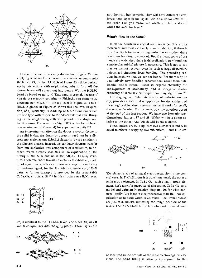
85

One more conclusion easily drawn from Figure 25, one applying what we know: when the clusters assemble into the lattice 83, the five LUMOs of Figure 25 will be pushed up by interactions with neighboring cube sulfurs. All the cluster levels will spread out into bands. Will the HOMO band be broad or narrow? That band is crucial, because if you d o the electron counting in PbMo6S8 you come to 22 electrons per [Mo6S8lZQ; the top level in Figure 25 is half- filled. A glance at Figure 25 shows that the level in question, of eg symmetry, is made up of Mo d functions which are of 6 type with respect to the Mo-S external axis. Bring- ing in the neighboring cells will provide little dispersion for this band. The result is a high DOS at the Fermi level, one requirement (of several) for s u p e r c o n d u ~ t i v i t y . ~ ~ ~ ~

An interesting variation on the donor-acceptor theme in the solid is that the donor or acceptor need not be a discrete molecule, as one [Mo6Ss] cluster is toward another in the Chevrel phases. Instead, we can have electron transfer from one sublattice, one component of a structure, to another. We’ve already seen this in the explanation of the tuning of the X-X contact in the AB2X2 ThCr2Si2 structure. There the entire transition metal or B sublattice, made up of square nets, acts as a donor or acceptor, a reducing or oxidizing agent, for the X sublattice, made up of X-X pairs. A further example is provided by the remarkable CaBezGe2 structure, 86.f411 In this structure one BzXz layer,

Ca 0 Be 0 86 Ge

87, is identical to the ThCr2Si2 layer. The other, 88, has B and X components interchanging places. These layers are

87

88

874

o x O B

o x 0 0

not identical, but isomeric. They will have different Fermi levels. One layer in the crystal will be a donor relative to the other. Can you reason out which will be the donor, which the acceptor layer?

What’s New in the Solid?

If all the bands in a crystal are narrow (as they are in molecular and most extremely ionic solids), i.e., if there is little overlap between repeating molecular units, then there is no new bonding to speak of. But if at least some of the bands are wide, then there is delocalization, new bonding; a molecular orbital picture is necessary. This is not to say that we cannot recover, even in such a large-dispersion, delocalized situation, local bonding. The preceding sections have shown that we can see bonds. But there may be qualitatively new bonding schemes that result from substantial delocalization. Recall in organic chemistry the consequences of aromaticity, and in inorganic cluster chemistry of skeletal electron-pair counting

The language of orbital interactions, of perturbation theory, provides a tool that is applicable for the analysis of these highly delocalized systems, just as it works for small, discrete, molecules. For instance, take the question posed at the end of the last section. We have two isomeric two- dimensional lattices, 87 and 88. Which will be a donor relative to the other? And which will be most stable?

These lattices are built up from two elements B and X in equal numbers, occupying two sublattices, I and I 1 in 89.

=I3 - - I

- E =

a b 09

The elements are of unequal electronegativity, in the general case. In ThCr,Si2, one is a transition metal, the other a main-group element, in CaBe2Ge2 each a main-group element. Let’s take, for purposes of discussion, CaBe2Ge2 as a model and write an interaction diagram, 90, for what happens locally (Ge is more electronegative than Be). No im- plication as to band width is yet made-the orbital blocks are just that, blocks, indicating the rough position of the levels. The lower block of levels is obviously derived from

90

0 M 0

Be BeGe@ GeQ

or localized in the orbitals of the more electronegative element. The band filling is actually appropriate to the

Angew. Chem. Int. Ed. Engl. 26 (1987) 846-878

CaBe,Ge-, structure, i.e., Be2Ge$', or BeGe', or seven electrons per two main-group atoms.

The orbitals develop into bands. The width of the bands depends on the inter-unit-cell overlap. The site I1 atoms are much farther apart from each other than the site I atoms (recall here the short metal-metal contacts in the ThCr2Si2 structure). We can say that sublattice I is more dispersive than sublattice 11. The orbitals of atoms placed in sublattice I will form wider bands than those in sublattice 11.

Now we have two choices: the more electronegative atoms can enter the less dispersive sites (lattice 11) or the more dispersive sites (lattice I). The consequences are shown in 91 and 92.

elements the binding energy gained in donor-acceptor in- teriuyer interactions overcomes the inherent stability of one isolated

At times the perturbation introduced by delocalization may be strong enough to upset the local, more "chemical" bonding schemes. Let me sketch two examples here.

Marcasites and arsenopyrites are a common structural choice for MAZ compounds, where M is a late transition metal and A an element of the fifth or sixth main group. The structure, 93, is related to the rutile one, in that one can easily perceive in the structure the octahedral coordination of the metal and one-dimensional chains of edge- sharing octahedra. The ligands are now interacting, however; not isolated 02' as in rutile, but S:" or P;" diatomic units in the m a r c a ~ i t e s . [ ~ ~ ]

A D

91 92

Which layer will be most stable and which will have the higher Fermi level depends on the electron filling. For a case such as CaBe,Ge,, or in general where the lower band is more than half-filled, the more electronegative atom will prefer the less dispersive site (91) and that layer will have a higher ionization potential, be a poorer donor.

The stability conclusion bears a little elaboration. It is based on the same "overlap repulsion" argument that was behind the asymmetric splitting of hydrogen chain bands (Fig. 1). When orbitals interact, the antibonding combinations are more antibonding than the bonding ones are bonding [cf. Eq. (a)]. Filling antibonding combinations, filling the tops of widely dispersed bands, is costly in energy. Conclusions on stability, as is the case in molecular chemistry, depend strongly on the electron count. In this particular case if the lower band were less than half-filled, the conclusion would be reversed, the more electronegative element should prefer the more dispersive site.

For ThCr2Siz AB2X2 structures the conclusion we reach, that the more electronegative element should enter the less dispersive site, implies that for most cases the main-group X component will prefer the less dispersive, square-pyra- midal, sublattice I1 positions. In CaBe2Ge2, G e is more electronegative than Be. That means the layer in which the G e enters the more dispersive sites (the bottom layer in 86) should be a donor relative to the upper layer.

A reasonable question to ask is the following. If one layer (the acceptor layer) in CaBe2Ge2 is more stable than the other, the donor layer, why does the CaBezGez structure form at all? Why doesn't it go into a ThCr2Siz structure based on the acceptor layer alone? The answer lies in the balance of covalent and dative interactions; for some

93

Low dimensionality characterizes another set of MS2 sublattices, now in ternary structures of the type of KFeS2 or Na3Fe2S4.[44.451 In these molecules one finds one-dimensional MS, chains, consisting of edge-sharing tetrahedra (94).

91

In both of these structural types, characterized by their simplicity, the metal-metal separations are in the range (2.6-3.1 A) where reasonable men, or women, might disagree whether there is much metal-metal bonding. Cases with bridging ligands are ones in which real metal-metal bonding is particularly difficult to sort out from bonding through the bridge. Certainly the metal-metal bonding doesn't look to be very strong, if it's there at all. So a chemist would certainly start out from the local metal site environment, which is strikingly simple.

One would then predict a three-below-two orbital splitting at each metal in the octahedral marcasites and a two- below-three splitting in the tetrahedral MS, chains. The magic electron counts for a closed-shell low-spin structure should be then d6 for the octahedral 93, d4 for the tetrahedral 94. Forming the one-dimensional chains and then the three-dimensional structure will introduce some dispersion into these bands, one might reason. But not much-appropriate electron counts for semiconducting or non-magnetic behavior should remain d6 for 93 and d4 for 94.

The experimental facts are as follows: the d 6 marcasites and arsenopyrites are semiconducting, but, surprisingly, so are the d4 ones. Most of the AMS2 structures synthesized to date feature the metal atom in configurations between

Angew. Chem in1 Ed Engl 26 (1987) 846-878 875

d5 and d”’. The measured magnetic moments are anoma-

When calculations on these chains are carried out, one finds, to one’s initial surprise, that the octahedral marca- site structure has a band gap at d 4 as well as d6, and that the tetrahedral chain has a band gap at d 5 5 and not d4. It seems that local crystal field considerations don’t work. What in fact happens (and here the reader is referred to the detailed explanation in our paper^[^^.^^]) is that the local field is a good starting point, but that further delocaliz- ing interactions (and these are ligand-ligand and metal- ligand, and not so much metal-metal in the distance range considered) must be taken into account. The extended interactions modify the magic or gap electron counts that might be expected from just looking at the metal site symmetry.

In the preceding section, I outlined the orbital interactions that are operative in the solid state. These were the same ones as those that govern molecular geometries and reactivity. There is an interesting new feature in some solids, however. This is an interaction-induced rearrangement of the DOS around the Fermi level.

Suppose that one of the interacting orbital components is localized, with narrow bands, but it is interacting with a metallic sublattice, characterized by a reasonable DOS at the Fermi level. This is indicated schematically in 95. Per-

lously low.

haps it’s best to have a real example to think about. Con- sider an acetylene chemisorbed in low coverage on a Pt( 1 1 1) surface, 96. Here the discrete, narrow-band orbitals are the four n and n* levels of a low-coverage acetylene layer, and the band is the Pt d band, nearly filled.[46.471

,,*y’ 96

The most important two-electron bonding interactions that take place are between two of the acetylene n orbitals, no and no- (see 97) and the d band. n, and 71,. “point”

& , & A & 97

/ /

toward the surface, have greater overlap with metal orbitals, and they interact preferentially with different parts of the band, picking out those metal surface orbitals which have similar nodal patterns as the adsorbate. 98 shows this-in the “parallel bridging” geometry at hand the n,

orbital interacts better with the bottom of the surface z 2 band and the n,. with the top of that band.

Both of these interactions are primarily of type @ and @ (see 81 or 95), four-electron repulsive or two-electron attractive interactions. Actually, the energetic and bonding consequences are a little complicated: the z2-no interaction would be destabilizing if the antibonding component of this interaction remained filled, below the Fermi level. In fact, many z2-n, antibonding states are pushed above the Fermi level, vacated. This converts a destabilizing, four- electron interaction into a stabilizing two-electron one.

A counterpart to this interaction is @ in 95. Normally we would not worry about zero-electron interactions, because there is no “power” in them if there are no electrons. However, in the case of a metal with a continuous band of states, some of these levels-these are bonding combinations of n,. with the top of the zz band, as indicated in 98- come below the Fermi level and are occupied. There- fore, they also contribute to bonding the adsorbate to the surface.

It should be noted that a consequence of all of these interactions is not only strengthening of metal-acetylene bonding, but also a weakening of bonding within the acetylene and within the metal. Interaction means delocalization, which in turn implies charge transfer. Interactions 0-0 operate to depopulate n,, populate n,., both actions weakening the acetylene n bond. Removing electrons from the bottom of the z2 band and filling better the top of that band both result in a weakening of the R-Pt bond.

Interaction @, peculiar to the solid, is a reorganization of the states around the Fermi level as a consequence of primary interactions 0-0. Consider, for instance, the levels that are pushed up above the Fermi level as a result of interaction 0, the four-electron repulsion. One way to think about this is the following: the electrons d o not, in fact, go up past the Fermi level (which remains approximately constant), but are dumped at the Fermi level into levels somewhere in the solid. This is shown schematically in 99.

But where is “somewhere”? The electrons that come in come largely from regions that are not directly involved in the bonding with the adsorbate. In the case at hand, they may come from Pt bulk levels, from Pt surface atoms not

876 Rngew Chern. lnf. Ed. Engl 26 (1987) 846-878

EF

bulk filled

99

adsorbate metal d states donor states

involved with the acetylene, from the Pt atoms binding the acetylene, but from orbitals of these atoms not used in that binding. While the metal surface is a nice reservoir of such electrons, these electrons are not innocent of bonding. They are near the top of their respective band (see W), and as such are metal-metal antibonding. Thus interaction @ weakens bonding in the surface. Together with the afore- mentioned electron transfer effects of interactions @-@ it is responsible for adsorbate-induced surface reconstruction.

In general, non-dissociative chemisorption is a delicate balance between attractive surface-molecule bonding and the consequences of the very same interactions, which weaken bonds in the adsorbed molecule and in the surface. Dissociative chemisorption and surface reconstruction are just two extremes of one and the same phenomenon.

I have discussed a n example here of a surface reaction. A more detailed analysis of the theoretical aspects of surface science will be given elsewhere.[481 I bring this example in, because I want to make the point that surface chemistry and physics is not a thing unto itself, but also part of the wondrous continuum of molecular bonding that is chemistry. Surface science, a discipline in an exciting, ex- plosive growth phase over the last decade, occasionally ne- glects its connections to solid-state chemistry. It shouldn’t. Solid-state chemists should also take more advantage of what surface scientists have learned. Rather interestingly, the intellectual connection between surface science and discrete molecular chemistry has remained strong, perhaps because one component of surface chemistry, the adsorbate, is patently a molecule. The cluster-surface analogy has also served to bring together the literatures of surface science and organometallic chemistry.

From the perspective of orbital interactions, surfaces by themselves, and surfaces interacting with molecules, fit perfectly into a continuum of dimensionality of solid-state chemistry and physics. They are two-dimensional, half-solid, half-molecule extended systems-the same tools of orbital analysis apply to surfaces as to other solids.

So what’s new in the solid? My straw-man physicist friend thinking of superconductivity, charge and spin density waves, heavy fermions, solitons, nonlinear optical phenomena, ferromagnetism in its various guises-all the fascinating things of interest to him and that I’ve neglected- he might say “everything.” An exaggeration of what I’ve said in this paper is “not much.” There are interesting,

novel consequences of delocalization and wide-band formation, but even these can be analyzed in the language of orbital interactions.

It would not surprise anyone if the truth were somewhere in between. It is certainly true that I’ve omitted, by and large, the origins of most of the physical properties of the solid, especially those like superconductivity and ferromagnetism that are peculiar to that state of matter. Chem- ists will have to learn much more solid-state physics than I’ve tried to teach here if they are to understand these ob- servables, and they must understand them if they are to make rational syntheses. I have concentrated on the most chemical notion of all-the solid is a molecule, a big one, to be sure, but just a molecule. Let’s try to extract from the perforce delocalized picture of Bloch functions the cherni- cal essence, the bonds that determine the structure and reactivity of this large molecule. The bonds must be there.

My graduate students, postdoctoral associates, and senior visitors to the group are responsible both for teaching me solid-state physics and for implementing the algorithms and computer programs that have made this work possible. While in my usual way I’ve suppressed the computations in favor of explanations, little understanding would have come without those computations. An early contribution to our work was made by Chien-Chuen Wan, but the real computational and interpretational advances came through the work of Myung- Hwan Whangbo, Charles Wilker, Miklos Kertesz, Tim Hughbanks, Sunil Wgeyesekera. and Chong Zheng. This paper owes much to their ingenuity and perseverance. Sev- eral crucial ideas were borrowed early on from Jeremy Bur- dett, such as using special k point sets for properties. Contri- butions were also made by Christian Minot. Jean- Yves Sail- lard, Denis Underwood, Georges Trinquier, Santiago Alvar- ez. Joel Bernstein, Jerome Silvestre, Marja Zonnevylle, Ralph Wheeler, Shen-shu Sung, Wolfgang Tremel. Douglas Keszler, and Jing Li.

In the early stages ofthis work, very important to me was a renewed collaboration with R. B. Woodward, prompted by our joint interest in organic conductors. It was unfortunately cut short by his death in 1979. Mike Sienko and his students offered gentle encouragement by showing us the interesting structures they worked on, as did Thor Rhodin on the surface science side. It was always instructive to try to provoke John Wilkins.

Over the years my research has been steadily supported by the National Science Foundation ’s Chemistry Division. I owe Bill Cramer and his fellow program directors thanks for their continued support. A special role in my group’s research on extended structures has been played by the Materials Science Center (MSC) at Cornell University, supported by the Mate- rials Research Division of the National Science Foundation. The MSC’s activities, especially the interdisciplinary semi- nars it has supported, and in general the opportunity is has offered for learning of work in other areas of science relevant to this topic, have been crucial in the development of my work. My recent surface work, briefly mentioned in the last section, has been generously supported by the OfJice of Naval Research.

One reason it is easy to cross disciplines at Cornell is the existence of the Physical Sciences Library, with its broad coverage of chemistry and physics. I would like to thank Ellen Thomas and her staff for her contributions here. Our draw- ings, a criticalpart of the way our research ispresenied, have

Angew. Chem. Inr. Ed. Engl. 26 (1987) 846-878 877

been beautifully made over the years by Jane Jorgensen and Elisabeth Fields. I‘d like to thank Eleanor Stagg for the typ- ing and secretarial assistance in the past, and Linda Kapi- tany for the present manuscript.

171is manuscript was written while I held the Tage Erlan- der Professorship of the Swedish Science Research Council NFR. The hospitality of Professor Per Siegbahn and the staff of the Institute of Theoretical Physics of the University of Stockholm is gratefully acknowledged, as well as the assistance of Ralph Wheeler, Jing Li, and Wolfgang Tremel in the writing and compulations. The comments of many people on this paper were also very useful, especially those of J . Dunitz and H.-G. von Schnering. I thank W . Tremel and H . Tremel for the German translation.

Received: March 5, 1987 [A 633 IE] German version: Angew. Chem. 99 (1987) 871

[I] a) E. Zintl, G. Woltersdorf, 2. Elektrochem. Angew. Phys. Chem. 41 (1935) 876; E. Zintl, Angew. Chem. 52 (1939) I ; b) W. Klemrn, E. Bus- mann, Z. Anorg. Allg. Chem. 319 (1963) 297; W. Klemrn, Proc. Chem. Sac. London 1958. 329; c) H. Schafer, B. Eisenmann, W. Muller, Angew. Chem. 85 (1973) 742; Angew. Chem. Int. Ed. Engl. 12 (1973) 694; d) H. Schafer, Annu. Rev. Mater. Sci. I S (1985) I , and references cited therein.

121 a) J. K. Burdett, NaturelLondon) 279 (1979) 121; b) in A. Navrotsky, M. OKeeffe (Eds.): Structure and Bonding in Crystals, Academic Press, New York 1981, p. 255; c) Acc. Chem. Res. I5 (1982) 34, and references cited therein.

131 J. K. Burdett, Prog. Solid State Chem. I5 (1984) 173. [4] a) M:H. Whangbo in J. S . Miller (ed.): Extended Linear Chain Com-

pounds, Plenum, New York 1982, p. 127; b) Acc. Chem. Res. 16 (1983) 95, and references cited therein.

151 M.-H. Whangbo in J. Rouxel (ed.): Crystal Chemistry and Properties of Materials with Quasi-One Dimensional Structures, Reidel, Dordrecht 1986, p- 27.

[6] The modern classic solid-state physics text is by N. W. Ashcroft and N. D. Mermin: “Solid State Physics,” Holt, Rinehart and Winston, New York, 1976. Three other introductions to the field, ones which I think are pedagogically effective and accessible to chemists are: W. A. Harrison: Solid State Theory, Dover, New York 1980; W. A. Harrison: Electronic Structure and the Properties of Solids, Freeman, San Francisco 1980; S . L. Altman: Band Theory oJMetals, Pergamon, New York 1970.

[7] Excellent introductions to this subject, written in the spirit of this article, and with a chemical audience in mind, are to be found in 13, 5, 8.1; M. Kertesz, Inf. Rev. Phys. Chem. 4 (1985) 125.

[8] T. A. Albright, J. K. Burdett, M.-H. Whangbo: Orbital Interactions in Chemistry. Wiley-Interscience, New York 1985, Chap. 20.

[9] For a review of this fascinating class of materials, see J. R. Williams, Ado. Inorg. Chem. Radiochem. 26 (1983) 235.

(101 F. A. Cotton, R. A. Walton: Multiple Bonds Between MetalAtoms. Wiley, New York 1982, and references cited therein.

[ I I ] For more information on the cyanoplatinates, see 14, 51. [I21 Fore more on the electronic structure of rutile and related compounds,

see: J. K. Burdett, T. Hughbanks, Inorg. Chem. 24 (1985) 1741; J . K. Burdett, ibid. 24 (1985) 2244; L. F. Mattheis, Phys. Reu. B: Solid State 13 (1976) 2433.

[ I ) ] J. B. Goodenough: Magnefrsm and the Chemical Bond, Krieger, New York 1976.

1141 R. S . Mulliken, J. Chem. Phys. 23 (1955) 1833, 2343. [IS] For this task, and for band structure calculation in general, a chemist

needs to learn group theory in the solid state. For a lucid introduction, see M. Tinkham: Group Theory and Quantum Mechanics. McGraw-Hill, New York 1964; G. Burns, A. M. Glazer: Space Groups.for Solid State Scientists, Academic Press, New York 1978; 0. Madelung: Introduction to Solid State Theory, Springer, Berlin 1978.

[16] The extension of overlap population considerations to the solid seems obvious, but 1 think we first introduced the formalism: a) T. Hughbanks, R. Hoffmann, J. Am. Chem. Sac. I05 (1983) 3528; b) S. D. Wijeyesekera, R. Hoffmann, Organometallics 3 (1984) 949; c) M. Kertesz, R. Hoff- mann, ibid. 3 (1984) 949; c) M. Kertesz, R. Hoffmann, J. Am. Chem. Sac. I06 (1984) 3453.

1171 This is from an extended Huckel calculation: J.-Y. Saillard, R. Hoff- mann, J. Am. Chem. Soc. 106 (1984) 2006 For better calculations, see 135).

[I81 This drawing was taken from [8]. [I91 Original reference: H. A. Jahn, E. Teller, Proc. R . Soc London Ser. A 161

(1937) 220: a discussion of the utility of this theorem in deriving molecular geometries is given by J. K. Burdett: Molecular Shapes, Wiley, New York 1980; Inorg. Chem. 20 (1981) 1959, and references cited therein; see also 13, 51 and R. G. Pearson: Symmetry Rulesfor Chemical Reac- tions. Wiley, New York 1976. The first application of the Jahn-Teller argument to stereochemical problems, and, incidentally, to condensed phases, was made by J. D. Dunitz, L. E. Orgel, J. Phys. Chem. So1id.s 3 (1957) 20, 318; Adv. Inorg. Chem. Rodiochem. 2 (1960) I ; L. E. Orgel, J . D. Dunitz, Nature (London) 179 (1957) 462. R. E. Peierls: Quantum 7heor.v of Solids. University Press, Oxford 1972. H. C. Longuet-Higgins, L. Salem, Proc. R. SOC. London Ser. A 251 (1959) 172. Review: M. Kertesz, Adu. Quantum Chem. 15 (1982) 161. W. B. Pearson, 2. Kristallogr. 171 (1985) 23, zit. Lit. For a theoretical analysis or this structural class, see: W. Trernel, R. Hoffmann, J. Am. Chem. Soc. 109 (1987) 124; Inorg. Chem. 26 (1987) 118; D. A. Keszler, R. Hoffmann, J. Am. Chem. Sac. I09 (1987) 118. F. Hulliger, R. Schmelczer, D. Schwarzenbach, J . Solid State Chem. 21 (1977) 371. R. Schmelczer, D. Schwarzenbach, F. Hulliger, Z . Naturforsch. 8 3 6 (1981) 463, and references cited therein. a) J. K. Burdett, P. Haaland, T. J. McLarnan, J. Cheni. Phys. 75 (1981) 5774; b) J. K . Burdett, S. Lee, J. Am. Chem. SOC. I05 (1983) 1079; c) J. K. Burdett, T. J. McLarnan, J. Chem. Phys. 75 (1981) 5764. a) M. C. Zonnevylle, R. Hoffmann, Langmuir 3 (1987). in press; b) G. Trinquier, R. Hoffmann, J. Phys. Chem. 88 (1984) 6696; c) J. Li. R. Hoff- mann, 2. Naturforsch. 8 4 1 (1986) 1399; d) P. B. Littlewood, CRC Crit. Rev. in Solid State Mat. Sci. I 1 (1984) 229. a) W. Tremel, R. Hoffmann, J. Am. Chem. SOC. I08 (1986) 5174, and references cited therein; b) J Silvestre, W. Tremel, R. Hoffmann, J. Less Common Met. 116(1986) 113. H. F. Franzen, T. 1. Burger, J. Chem. Phys. 49 (1968) 2268; H. F. Franz- en, G. A. Wiegers, J. Solid State Chem. 13 (1975) I 14. For further elaboration, see [16c, 291. W. B. Pearson, J . Solid State Chem. 56 (1985) 278, and references cited therein. A. Mewis, 2. Naturforsch. 8 3 5 (1980) 141. a ) C. Zhene. R. Hoffmann. J. Phvs. Chem 89 (19851 4175: bl Z . Natur- - . I ~, . , forsch. 8 4 1 (1986) 292; c) J. Am. Chem. Sac. 108 (1986) 3078.

[35] 0. K. Andersen in P. Phariseau, W. M. Ternrnerman (Eds.): The Elec- tronic Structure ofcomplex Systems. Plenum, New York 1984; in F. Bas- sani, F. Fumi, M. P. Tossi (Eds.): Highlights of Condensed Matter Phy- sics. North-Holland, New York 1985.

j361 J. N. Murrell, M. Randic, D. R. Williams, Proc. R Sac. London Ser. A284 (1965) 566; A. Devaquet, L. Salem, J. Am Chem. SOC. 91 (1969) 379; K. Fukui, H. Fujimoto, Bull. Chem. Sac. Jpn. 41 (1968) 1984; M. Baba, S. Suzuki, T. Takemura, J. Chem. Phys. 50 (1969) 2078; M.-H. Whangbo, S. Wolfe, Can. J. Chem. 54 (1976) 949; K . Morokuma, J. Chem. Phys. 55 (1971) 1236.

[37] Review: R. Chevrel in S. Foner, B. B. Schwartz (Eds.): Superconductor Materials Science: Metallurgy. Fabrication and Applications, Plenum, New York 1981, Chap. 10.

[38] L H . Lin, J. K. Burdett, Inorg. Chem. 21 (1982) 5. 1391 T. Hughbanks, R. Hoffmann, J. Am. Chem. Sac. 105 (1983) 1150. 1401 See also 0. K. Andersen, W. Klose, H. Nohl, Phys. Reu. 8: Solid State 17

(1977) 1760; H. Nohl, W. Klose, 0. K. Andersen in 0. Fisher, M. B. Maple (Eds.): Superconductivity in Ternary Compounds, Springer, Berlin 1981, Chap. 6 ; D. W. Bullett, Phys Rev. Lett. 44 (1980) 178.

[41] See [34c], and references cited therein. (421 K. Wade, Chem Commun. 1971. 792; Inorg. Nucl. Chem. Lett. 8 (1972)

559; Electron Deficient Compounds, Nelson, London 1971; D. M. P. Mingos, Nature (London) Phys. Sci. 236 (1972) 99.

1431 For references, see S. D. Wijeyesekera, R. Hoffmann, Inorg. Chem. 22 (1983) 3287.

[44] W. Bronger, Angew. Chem. 93 (1981) 12; Angew. Chem Int. Ed. Engl. 20 (198 I ) 52.

1451 J. Silvestre, R. Hoffmann, Inorg. Chem. 24 (1985) 4108. 1461 J . Silvestre, R. Hoffmann, Langmuir I (1985) 621. (471 The general principles underlying orbital interactions in chemisorption

were analyzed also in our earlier paper on C-H and H-H activation [171.

I481 R. Hoffmann, Rev. Mod. Phys.. in press.


How Chemistry and Physics Meet in the Solid State · How Chemistry and Physics Meet in the Solid State By Roald Hoffmann* To make sense of the marvelous electronic properties of the

Documents