Journal of Housing Economics 10, 335–362 (2001) doi:10.1006/jhec.2001.0294, available online at http://www.idealibrary.com on Housing and Labor Supply 1 Edwin Deutsch Institute for Econometrics, University of Technology—Vienna, Argentinierstrasse 8, A-1040 Vienna, Austria E-mail: [email protected] Website: www.eos.tuwien.ac.at/Oeko/EDeutsch/ Norbert Neuwirth OIF (Austrian Institute for Family Studies), Gonzagagasse 19, A-1010, Vienna, Austria E-mail: [email protected] and Askin Yurdakul Institute for Econometrics, University of Technology—Vienna, Argentinierstrasse 8, A-1040 Vienna, Austria Received January 31, 2001 Dedicated to the memory of Steve Mayo The types and risks of life-styles and their impact on labor and housing markets raise increasing attention. We address the question how people allocate their work effort under a given structure of incomes according to family status, skills, tenure, and cost. The interplay between work hours supply, income uncertainties, gender-specific skill levels, and spatial differentiation is investigated by means of econometric models that are parsimo- nious in structure. Up to certain limits the scale of income uncertainties explains work effort in partnerships and among singles. Mating of skills in partnerships likely plays a decisive role how incomes are pooled to cover housing costs. q 2001 Elsevier Science 1. INTRODUCTION The types and risks of life-styles and their impact on labor and housing markets raise increasing attention. This paper attempts to provide further empirical evidence. It addresses the question how people allocate their work effort in a given structure of incomes according to family status, skill, tenure, and housing cost. 1 A previous version of this paper was presented at the joint ENHR–AREUEA conference in Ga ¨vle, Sweden, June 2000. Financial support from the Austrian Jubila ¨ums-Fund (Project 6004) is gratefully acknowledged. Thanks go to the Austrian Statistical Institute for data support. Special thanks for valuable comments go to the anonymous referee. 335 1051-1377/01 $35.00 q 2001 Elsevier Science All rights reserved.

Welcome message from author
This document is posted to help you gain knowledge. Please leave a comment to let me know what you think about it! Share it to your friends and learn new things together.
Transcript
Journal of Housing Economics 10, 335–362 (2001)
doi:10.1006/jhec.2001.0294, available online at http://www.idealibrary.com on
Housing and Labor Supply1
Edwin Deutsch
Institute for Econometrics, University of Technology—Vienna,Argentinierstrasse 8, A-1040 Vienna, Austria
E-mail: [email protected]: www.eos.tuwien.ac.at/Oeko/EDeutsch/
Norbert Neuwirth
OIF (Austrian Institute for Family Studies), Gonzagagasse 19, A-1010, Vienna, AustriaE-mail: [email protected]
and
Askin Yurdakul
Institute for Econometrics, University of Technology—Vienna,Argentinierstrasse 8, A-1040 Vienna, Austria
Received January 31, 2001
Dedicated to the memory of Steve Mayo
The types and risks of life-styles and their impact on labor and housing markets raiseincreasing attention. We address the question how people allocate their work effort undera given structure of incomes according to family status, skills, tenure, and cost. Theinterplay between work hours supply, income uncertainties, gender-specific skill levels,and spatial differentiation is investigated by means of econometric models that are parsimo-nious in structure. Up to certain limits the scale of income uncertainties explains workeffort in partnerships and among singles. Mating of skills in partnerships likely plays adecisive role how incomes are pooled to cover housing costs. q 2001 Elsevier Science
1. INTRODUCTION
The types and risks of life-styles and their impact on labor and housingmarkets raise increasing attention. This paper attempts to provide further empiricalevidence. It addresses the question how people allocate their work effort in a givenstructure of incomes according to family status, skill, tenure, and housing cost.
1A previous version of this paper was presented at the joint ENHR–AREUEA conference in Gavle,Sweden, June 2000. Financial support from the Austrian Jubilaums-Fund (Project 6004) is gratefullyacknowledged. Thanks go to the Austrian Statistical Institute for data support. Special thanks forvaluable comments go to the anonymous referee.
335
1051-1377/01 $35.00q 2001 Elsevier Science
All rights reserved.
336 DEUTSCH, NEUWIRTH, AND YURDAKUL
The issue of tenure choice under income uncertainty is of course an old theme.The conventional wisdom is that individuals facing higher income uncertaintyare less likely to be or to become home owners. In the 1990s the hypothesis waschallenged by contradictory results. In order to shed light on the issue Robst etal. (1999) investigated several measures for income uncertainty. They foundsome evidence for lower ownership rates among movers with higher incomeuncertainty and pointed out that the uncertainty effects may even exceed theincome effects.
Although tenure choice as such will not be investigated here, the incomeuncertainties faced by genders will play a central role. Similar to wealth, humancapital endowments do not only enhance the ability for borrowing against future,they also affect locational choice. In that respect the recent literature offers avariety of interesting avenues.
One point of view is the mating process between genders of different skilllevels and local job opportunities, the so-called colocation problem. In a recentcontribution Costa and Kahn (2000) investigated the longer-term and dispropor-tionate increase in college-educated “power” couples living in U.S. metropolitanareas. Drawing from econometric estimates they argued that the skill upgradingis driven by job matching, which educated women find easier to solve in metropol-itan areas.
On similar lines we investigate the labor supply decisions in mating categoriesalong gender-specific skill levels. The estimates show that the effects muchdepend on the skill-mating categories; moreover they suggest that some part ofthe skill-upgrading process is driven by spatial differentiation. By augmentingdemographic traits with locational choice we follow the recommendations ofGabriel and Rosenthal (1999).
Some caution is necessary because our results cannot be viewed independentlyof the spatial organization of a society. As emphasized by van Ommeren et al.(1999) locational choice should be based on the geographical structure of aneconomy. They argue that in the Netherlands, being a small country, residentialand job mobility are rather independent conditions on commuting costs, gettingcorrelated only with larger distances when life-time utility is probably at stake.We want to add that locational choice should also be seen in conjunction withhousing politics; the Austrian housing policies favor home ownership formationin smaller settlements on a par with urban renewal where renting is dominant.This in turn contributes to city amenities which attract the higher skills.
Apart from interpretative issues the paper essentially centers upon modelingthe interplay between work hours supply, income uncertainties related to housinglife-styles, gender-specific skill levels, and spatial differentiation. Our approachis modest as we proceed by inductive logic from evidence to test. The econometricmodels offered below are explicitely simple and parsimonious in structure. Theonly implicit albeit not innocent assumption is separability between housing andother consumption, which means that for given wages any change in income
HOUSING AND LABOR SUPPLY 337
uncertainty does not affect the structure of housing through induced demand (forseparability concepts, see Deaton and Muellbauer (1980), among others).
The database is the Austrian census over subsequent years, restricted to theAustrian population in the work force, i.e., without non-Austrian permanentresidents and without householders in retirement. The database is rich both insample size and in characteristics about family status, work status, and tenure.Unfortunately, data about assets and mortgages in ownership are lacking andownership costs are rather qualitative. This restricts the scope of modeling aswe had to develop a concept of income uncertainty over low versus high housingcost categories. Instead the many informations on skill levels permit a thoroughanalysis of labor supply in partnerships and single-person households, in conjunc-tion with income levels and uncertainties.
The paper is organized as follows. Section 2 offers a summary of the methodput forward in this paper. The subsequent three sections describe the major piecesof empirical evidence: Section 3 decomposes the incomes into age-dependentpermanent profiles and residual income ratios which reveal the income uncertain-ties over the life-cycle; Section 4 discusses the distribution of hours of workand wages per hour, which conducts the subsequent tests for work sharing inpartnerships; and Section 5 derives a rank order of gender-specific income uncer-tainties related to housing. In Section 6 we estimates the probabilities for femalelabor market participation in conjunction with spatial differentiation, by applyingbivariate Probit. Section 7 turns to a 3SLS model, which estimates the simultane-ous choice of work hours in partnerships. Section 8 offers OLS estimates forsingles, a large population that appears somewhat neglected by econometricresearch. The paper ends with conclusions and references. The Appendix con-taining model formulas and estimates can be downloaded from www.eos.tuwien.ac.at/Oeko/EDeutsch/JHE.html/
2. A FRAMEWORK FOR MODELING AND ESTIMATION
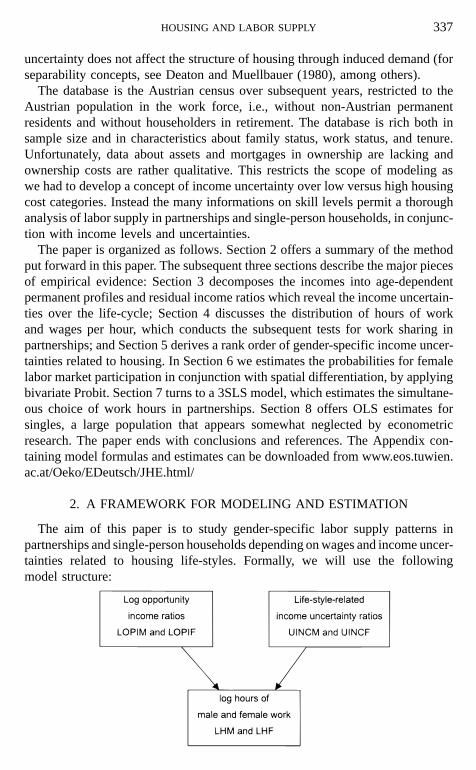
The aim of this paper is to study gender-specific labor supply patterns inpartnerships and single-person households depending on wages and income uncer-tainties related to housing life-styles. Formally, we will use the followingmodel structure:
338 DEUTSCH, NEUWIRTH, AND YURDAKUL
The log income ratios LOPIM and LOPIF are defined as the logs of the ratiosbetween actual and predicted incomes where the latter are drawn from agedependent income profiles; the income uncertainty ratios UINCM and UINCFare the spread between the 80% and the 20% income quantile in percentages ofthe median income within social groups. The hours of work are measured perweek. Together with informations on gender-specific labor participation we willestimate linear models of the type
LHM 5 b*LOPIM 1 p *UINCM 1 Xu 1 . . .(1)
LHF 5 c*LOPIF 1 q*UINCF 1 Xu 1 . . . ,
where b, c, p, and q are elasticities and X denotes the set of other explanatorieswith parameter vector u. The equations are estimated separately for male andfemale single-person households; for partnerships the equations are pooled intoa simultaneous two-equation system.
Although models of this type can be justified from adjustment costs andexpected utility analysis, we develop the basic ideas from available evidence.
One main tool of analysis is indeed the notion of housing life-style-relatedincome uncertainty, or income uncertainty for short. The social groups underconsideration are categorized by gender, family status, age, tenure, and low versushigh housing costs. As discussed below, the statistics on income uncertainty arederived from pooled cross-section surveys. Longitudinal data in a proper senseare unavailable in Austria. Thus the income uncertainty as used in this paper isno individual datum but rather some fundamental characteristic of the socialgroup to which a household belongs. Given an appropriate classification ofhouseholds this statistic can serve as a proxy for individual income volatility.Beyond that it may offer additional information about social group behavior. Tosee this, consider local traditions, habits, regional markets, local job-matchingopportunities, and unemployment rates, which all determine the local welfareconditions together with the level and the variability of household income overspace and time. In this sense the uncertainty statistic is drawn from the space offeasible earning states; these in turn widen or restrict the scope of individual laborsupply decisions, depending on risk attitudes and other household characteristics.
We are particularly interested to include housing characteristics into the set ofattributes. The life-styles we investigate manifest themselves in tenures, locations,and affordability conditions that categorize the social groups over which incomeuncertainty is evaluated. In exactly this sense we postulate housing lifestyles asa central factor that influences individual labor supply. Housing plays thereforea prominent role in our analysis, even if its characteristics remain somewhatconcealed in the income statistics we are going to use.
The basic hypothesis we put forward can be stated now. We claim that differentincome uncertainties permit or request higher or lower work efforts over the life
HOUSING AND LABOR SUPPLY 339
cycle; i.e., the work hours elasticities of uncertainty p and/or q are significant,given risk attitudes.
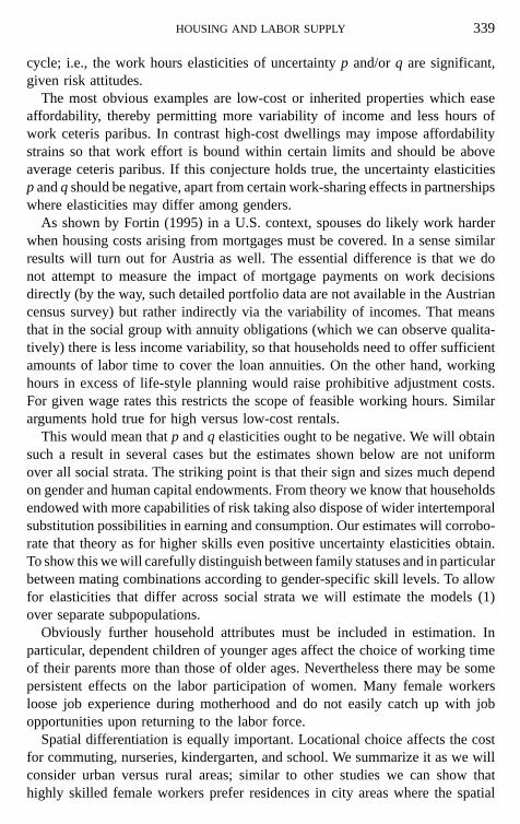
The most obvious examples are low-cost or inherited properties which easeaffordability, thereby permitting more variability of income and less hours ofwork ceteris paribus. In contrast high-cost dwellings may impose affordabilitystrains so that work effort is bound within certain limits and should be aboveaverage ceteris paribus. If this conjecture holds true, the uncertainty elasticitiesp and q should be negative, apart from certain work-sharing effects in partnershipswhere elasticities may differ among genders.
As shown by Fortin (1995) in a U.S. context, spouses do likely work harderwhen housing costs arising from mortgages must be covered. In a sense similarresults will turn out for Austria as well. The essential difference is that we donot attempt to measure the impact of mortgage payments on work decisionsdirectly (by the way, such detailed portfolio data are not available in the Austriancensus survey) but rather indirectly via the variability of incomes. That meansthat in the social group with annuity obligations (which we can observe qualita-tively) there is less income variability, so that households need to offer sufficientamounts of labor time to cover the loan annuities. On the other hand, workinghours in excess of life-style planning would raise prohibitive adjustment costs.For given wage rates this restricts the scope of feasible working hours. Similararguments hold true for high versus low-cost rentals.
This would mean that p and q elasticities ought to be negative. We will obtainsuch a result in several cases but the estimates shown below are not uniformover all social strata. The striking point is that their sign and sizes much dependon gender and human capital endowments. From theory we know that householdsendowed with more capabilities of risk taking also dispose of wider intertemporalsubstitution possibilities in earning and consumption. Our estimates will corrobo-rate that theory as for higher skills even positive uncertainty elasticities obtain.To show this we will carefully distinguish between family statuses and in particularbetween mating combinations according to gender-specific skill levels. To allowfor elasticities that differ across social strata we will estimate the models (1)over separate subpopulations.
Obviously further household attributes must be included in estimation. Inparticular, dependent children of younger ages affect the choice of working timeof their parents more than those of older ages. Nevertheless there may be somepersistent effects on the labor participation of women. Many female workersloose job experience during motherhood and do not easily catch up with jobopportunities upon returning to the labor force.
Spatial differentiation is equally important. Locational choice affects the costfor commuting, nurseries, kindergarten, and school. We summarize it as we willconsider urban versus rural areas; similar to other studies we can show thathighly skilled female workers prefer residences in city areas where the spatial
340 DEUTSCH, NEUWIRTH, AND YURDAKUL
residential–job matching problem can be solved easier than in remote parts ofthe country.
Given these preliminaries the empirical part of the paper starts with evidencedrawn from Austrian data. The basic evidence is offered in three steps.
The first piece of evidence concerns the personal and household income profilesover the life-cycle, see Section 3. Using a modified Mincer approach, the profilesare estimated for separate skill levels. Following the usual notation the predictedprofiles are labeled permanent income. The ratios between the observed and thepredicted incomes OPIM and OPIF are interpreted as opportunity income ratiosof male and female workers, respectively. Since their dispersion increases withage, this outcome mirrors the stylized fact that the job risks increase toward theage of retirement.
The second piece of evidence is statistics about gender-specific hours of workand wages per hour, see Section 4. We separate employed couples from single-person households, labeled singles for short, leaving other household types aside.The statistics of employed couples suggest that hours of work sharing in partner-ships is widespread, even in such a way that couples tend to optimize their totalworking time conditional upon gender-specific wage opportunities. It is alsonoted that female workers generally display more dispersion of hours of workeven if that effect is much weaker among singles than among married women.Thus also among female singles we should expect some impact of income uncer-tainty on hours of work.
The third piece of evidence is the cornerstone of analysis, i.e., the pattern ofincome levels and uncertainties across social groups. The sample of censusdata contains about 27,200 observations, which makes it possible to distinguishbetween 114 social categories altogether, see Section 5. Not surprisingly a positivecorrelation between housing cost and income level obtains. More interestinglyit turns out that the lower the housing cost the higher the income variability, upto certain limits. The negative correlation is significant for households (as units)but not so for individuals; while the income uncertainties of females UINCF canbe perfectly ranked according to the cost of housing life-styles, the effect is muchweaker for males. However, consistent with the income profiles the incomeuncertainties UINCM and UINCF increase with age.
Summing up these findings we maintain that income uncertainties do signifi-cantly influence the personal work effort needed to afford the chosen life-styles.The remainder of this paper is devoted to tests. Of course there are variousconceptual problems that cannot be addressed here, among others hours restric-tions set by labor demand. So we focus on the following questions: Is thesharing of work hours uniform over all skill levels? How does self-selection ofnonparticipating female workers (housewives) affect the labor supply of malepartners? Finally, to which extent (if at all) is the outcome influenced by spatialdifferentiation and income uncertainties?
HOUSING AND LABOR SUPPLY 341
The strategy is to evaluate the inverse Mills ratios, which correct the self-selection bias from nonparticipation, while for singles we do not consider choiceproblems of that sort. Then we use (1) to estimate labor supply over seven matingcategories over skill levels in partnerships as well as for three skill levels ofmale and female singles.
3. INDIVIDUAL AND HOUSEHOLD INCOME PROFILES
The first piece of evidence concerns the decomposition of individual incomedata into a permanent (strata-specific) and a transitory (individual) component.The permanent component will be called an age-dependent income profile. Theprofiles under consideration are evaluated for
• PINCM and PINCF: personal gender-specific monthly net incomes ofmale/female householders and their partners (without social transfers but withunemployment benefits whenever reported), and
• INCOME: monthly net household incomes totaling the personal incomesof the householder and his/her partner, including family support. Personal incomesof other household members remain unconsidered.
The database is the Austrian census, pooled over the surveys from 1991 until1997, restricted to the population in the labor force, with 27,200 observationsaltogether. Cyclical and trend effects are filtered out by suitable estimation, soa full account of structural profiles over the 1990s obtains. The basic model isa modified Mincer-type weighted OLS model that allows for concave profiles:
log (INC) 5 a1*AGE 1 a3*AGE3 /1000 1 KOHk 1 Xu 1 u (2)
The symbol INC denotes the income variables PINCM, PINCF, and INCOMErespectively. The age is measured in years from labor force entry with PAGEM(males), PAGEF (females), and AGE (households). In order to avoid confusionwe will speak of personal age when referring to the individual’s age from birth.The constant term is replaced by the explanatories KOHk, which are fixed dum-mies over the subsequent entry decades –1969, 1970–1979, 1980–1989, 1990–,estimating starting incomes under unchanged economic environments. The setof explanatory variables summarized in X consists of
• skill level (low, middle, high),• family status (single, lone parent with dependents, partnerships 5 couples),• number of dependents, classified as small (#2 children) and large ($3
children),• employment type (private or public sector),
342 DEUTSCH, NEUWIRTH, AND YURDAKUL
• employment status (employed, unemployed), and• location: Urban–nonurban, with
Urban: cities (.50,000 inhabitants) and their regional environment.
The term u is the error term. Some collinearity problems in profile estimationare apparent, but it can be shown that the cubic term AGE3 does not only fitbetter but does also attenuate the collinearity biases arising from quadratic AGEterms: for details see the Appendix. Note that labor time, tenures, and housingcost levels are not included in estimation but treated as separate variables insubsequent models.
From the predictors PRED* of the age-dependent permanent income profileswe get the individual income ratios
OPIM 5 PINCM/PREDPINCM and OPIF 5 PINCF/PREDPINCF. (3)
The ratios account for the (uncompensated) opportunity costs of leisure of malesand females. For that reason we term them opportunity income ratios.
All profiles were estimated on separate samples according to skill. Followingcommon standards we used three categories constructed as a mix between school-ing and job experience:
• low-skill work (primary school education and unskilled work),• middle-skill work (all workers who are neither low skilled nor highly
skilled),• high-skill professions (academics or high school-educated with profes-
sional positions).
The skill level of individuals originates from the census data; the householdskill levels are maximum levels over householder and partner when belongingto the labor force (see Table I).
About two-thirds of the Austrian labor force falls into the middle-skill category.The share of low skill declined by more than 2% over the 1990s while the share
TABLE ISkill Levels for Individuals and Households in 1997
1997 survey Austria, all Austria, all Cities, all Cities, all Austria, allpercentage males in females in males in females in households
shares labor force labor force labor force labor force in labor force
Low skill 16.0 29.3 12.0 19.7 14.0Middle skill 69.8 60.9 63.9 65.0 70.4High skill 14.1 9.8 24.1 15.2 15.6
Total 100.0 100.0 100.0 100.0 100.0
HOUSING AND LABOR SUPPLY 343
of highly skilled professions increased by about the same amount. Similar figuresand tendencies are found for German workers, compare Franz (2000). The upgrad-ing of the skill levels was partly due to the substantial increase in female schooling,where skilled professions are predominantly found in the cities. Outside the citiesa still high share of low-skill female is apparent. Similar observations obtainedfor the United States stimulated a debate of explaining spatial differentiationthrough skill levels and related mating opportunities, see Costa and Kahn (2000),a topic to be considered below.
A full account of the profile estimates cannot be given here but found in aprevious conference paper by the same authors, see Deutsch et al. (2000). Forthe remainder of this section we confine ourselves to the major topic of interest,i.e., the age-dependent income dispersions around the profiles.
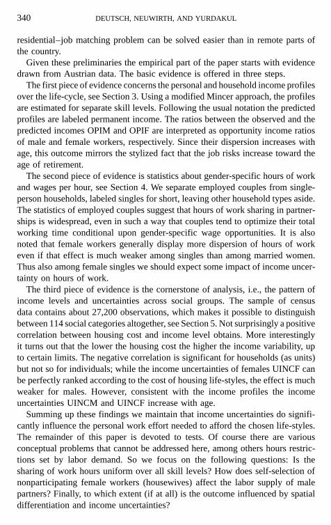
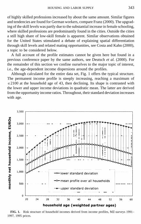
Although calculated for the entire data set, Fig. 1 offers the typical structure.The permanent income profile is steeply increasing, reaching a maximum ofP2100 at the household age of 43, then declining. Its shape is contrasted withthe lower and upper income deviations in quadratic mean. The latter are derivedfrom the opportunity income ratios. Throughout, their standard deviation increaseswith age.
FIG. 1. Risk structure of household incomes derived from income profiles, MZ-surveys 1991–1997, 1995 prices.

344 DEUTSCH, NEUWIRTH, AND YURDAKUL
There are various reasons for that. One source arises from unemployment. Byconstruction it is unemployment benefit divided by permanent income. Becauseunemployment rises with age it shows up in an increasing income dispersion.
Of course low-skill households are most affected by unemployment. In thisgroup the lower income deviations are relatively large. That low-cost housingmatters for them can be seen from their earnings profiles, which do not exceedP1600 per month; after the age of 40 they already start to decline. Instead theearnings of middle-skill households reach a maximum of P 2100 about 6 yearslater. Both profiles contrast with that of high-skill professions. The latter exerta real takeoff after the age of 35, reaching a maximum of P 3200 at the age of50 years. Unemployment among high skills is lower so that their asset planninghorizon—including intertemporal substitution of consumption through risk tak-ing—is likely more extended than that for lower skills.
Another factor of age-dependent income dispersions is the laborforce participa-tion of women. From the estimated cohort effects it can be deduced that thestarting wage differential between men and women has decreased over time. Forcomparable skills female starting wages were only 76% of their male counterpartsin the 1960s while reaching 84% in the 1990s. However, better starting conditionsdid not equally reduce the wage differentials. The main reasons are job interrup-tions and restricted career opportunities for women during and after motherhood.
4. MARKET WORK EFFORT AND WAGES
The second piece of evidence concerns the allocation of market work effortunder given market wages. At this point we must separate partnerships fromother types of households. Partners are in the position to share the risks of incomebetween themselves while lone householders—letting mixed housing groups withother income earners apart—do not have access to such an alternative.
Data mining in the Austrian census surveys yields the remarkable result thatin partnerships where both partners are employed there must be some tradeoffbetween male and female hours supplied per week.
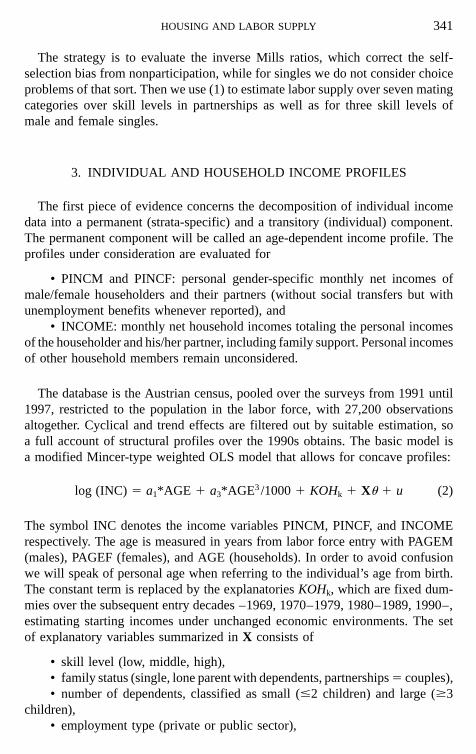
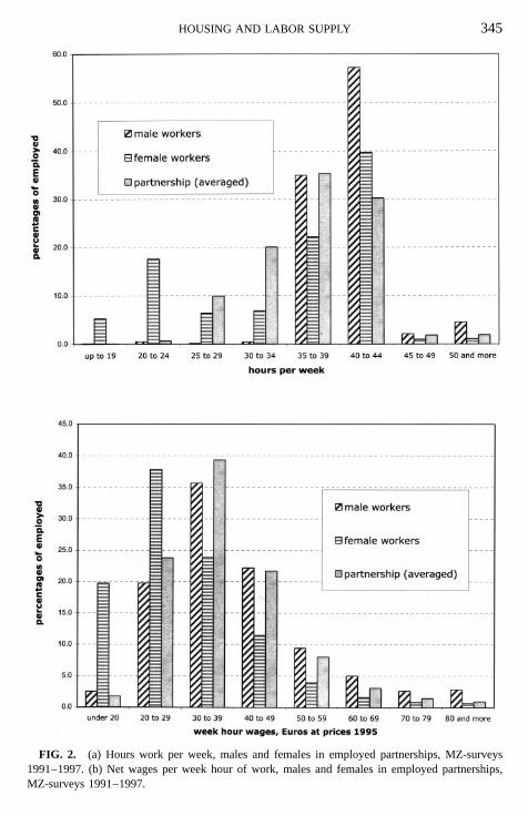
The statistics about the dispersion of work hours and wages are presented inFig. 2a and 2b, summary statistics following in Table II. Male and female workhours per week were retrieved from the original data set. Marginal employmentsof less than 9 h per week and inconsistent responses were removed from thesample. Work hours in partnerships were calculated by assigning the weight 1/2
to each partner. As a convenient measure we derived wages per week hour frommonthly net incomes divided by hours per week. The partnership wages perweek were defined as male plus female monthly income divided by male plusfemale work hours per week.
From Fig. 2a we see that hours per week of male workers perform an unimodaldistribution. No less than 92% of all men indicate a work load from 35 to 44 h
HOUSING AND LABOR SUPPLY 345
FIG. 2. (a) Hours work per week, males and females in employed partnerships, MZ-surveys1991–1997. (b) Net wages per week hour of work, males and females in employed partnerships,MZ-surveys 1991–1997.
346 DEUTSCH, NEUWIRTH, AND YURDAKUL
TABLE IIDistribution of Hours and Wage Rates among Employed Singles
Work hours Male Female Wages per Male Femaleper week workers workers weekly hours workers workers
up to 19 0.3 0.9 under 20 5.4 7.920 to 24 1.4 3.1 20 to 29 26.7 33.825 to 29 0.4 1.6 30 to 39 34.8 34.830 to 34 0.6 3.1 40 to 49 17.8 13.735 to 39 33.1 32.0 50 to 59 7.7 5.540 to 44 56.9 55.8 60 to 69 4.0 2.245 to 49 2.5 1.6 70 to 79 1.6 0.950 and more 4.8 1.9 80 and more 2.0 1.2
Total % 100.0 100.0 Total % 100.0 100.0Weighted mean 39.8 38.5 Weighted mean 37.7 34.4Standard deviation 5.3 5.7 Standard deviation 15.1 13.2
Partnerships, both employedWeighted mean 40.1 33.5 Weighted mean 41.0 30.4Standard deviation 4.2 9.2 Standard deviation 16.1 13.8
per week. In contrast the distribution for female workers is markedly bimodal.Only 61% of all women report work hours between 35 and 44 h. There is asecond peak with an 18% frequency of part-time work between 20 and 24 h.
The distribution of partnership work hours is unimodal. The frequency patternis a mix of the distributions of the genders, showing a dispersion in between thatof male and female partners. To generate such a shape there should be sufficientlymany partnerships combining 40 and 44 h male work with part-time work offemale partners, while sufficiently many females working above-average hoursshould combine their effort with male partners working below average.
Figure 2b shows the distribution of wages per weekly hours. The highestfrequency for female wage rates is observed over the interval [20,30) EUROs;for male wage rates it is [30,40) EUROs. The most interesting finding is themodal frequency of the partnership wage rates. A relative majority of 40% earns[30,40) EUROs. This frequency is higher than the modal frequencies for menand women separately. To generate such a shape there should be sufficientlymany partners combining above-average male wage rates with lower part-timefemale wage rates.
Loosely speaking the results suggest that work-hours sharing in partnershipsis widespread, even in such a way as couples tend to optimize total workingtime conditional upon available gender-specific wage opportunities.
To which extent does the gender-specific hours and wage pattern of singlesdiffer? Since the structure is much simpler, the distribution can be easily recog-nized from Table II. The distributions for singles are all unimodal. It is easily
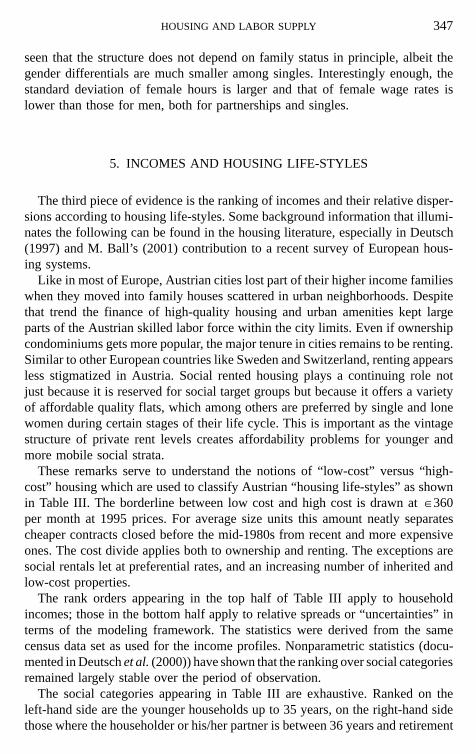
HOUSING AND LABOR SUPPLY 347
seen that the structure does not depend on family status in principle, albeit thegender differentials are much smaller among singles. Interestingly enough, thestandard deviation of female hours is larger and that of female wage rates islower than those for men, both for partnerships and singles.
5. INCOMES AND HOUSING LIFE-STYLES
The third piece of evidence is the ranking of incomes and their relative disper-sions according to housing life-styles. Some background information that illumi-nates the following can be found in the housing literature, especially in Deutsch(1997) and M. Ball’s (2001) contribution to a recent survey of European hous-ing systems.
Like in most of Europe, Austrian cities lost part of their higher income familieswhen they moved into family houses scattered in urban neighborhoods. Despitethat trend the finance of high-quality housing and urban amenities kept largeparts of the Austrian skilled labor force within the city limits. Even if ownershipcondominiums gets more popular, the major tenure in cities remains to be renting.Similar to other European countries like Sweden and Switzerland, renting appearsless stigmatized in Austria. Social rented housing plays a continuing role notjust because it is reserved for social target groups but because it offers a varietyof affordable quality flats, which among others are preferred by single and lonewomen during certain stages of their life cycle. This is important as the vintagestructure of private rent levels creates affordability problems for younger andmore mobile social strata.
These remarks serve to understand the notions of “low-cost” versus “high-cost” housing which are used to classify Austrian “housing life-styles” as shownin Table III. The borderline between low cost and high cost is drawn at P360per month at 1995 prices. For average size units this amount neatly separatescheaper contracts closed before the mid-1980s from recent and more expensiveones. The cost divide applies both to ownership and renting. The exceptions aresocial rentals let at preferential rates, and an increasing number of inherited andlow-cost properties.
The rank orders appearing in the top half of Table III apply to householdincomes; those in the bottom half apply to relative spreads or “uncertainties” interms of the modeling framework. The statistics were derived from the samecensus data set as used for the income profiles. Nonparametric statistics (docu-mented in Deutsch et al. (2000)) have shown that the ranking over social categoriesremained largely stable over the period of observation.
The social categories appearing in Table III are exhaustive. Ranked on theleft-hand side are the younger households up to 35 years, on the right-hand sidethose where the householder or his/her partner is between 36 years and retirement
348 DEUTSCH, NEUWIRTH, AND YURDAKUL
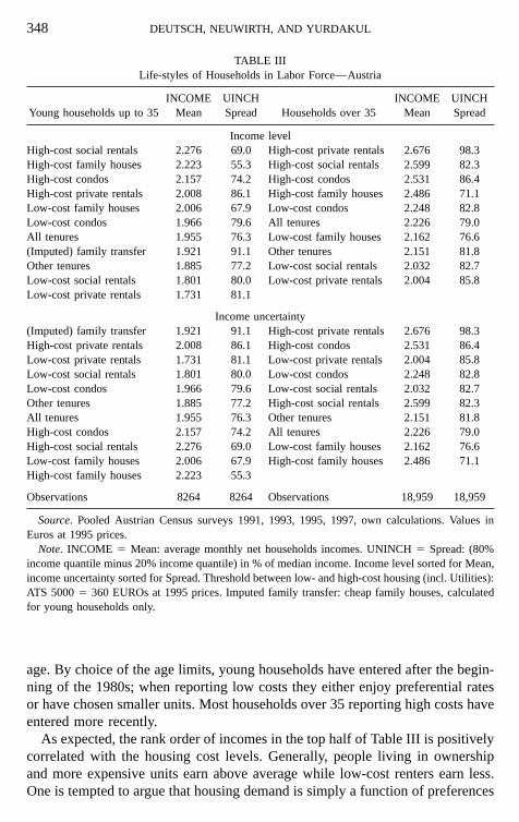
TABLE IIILife-styles of Households in Labor Force—Austria
INCOME UINCH INCOME UINCHYoung households up to 35 Mean Spread Households over 35 Mean Spread
Income levelHigh-cost social rentals 2.276 69.0 High-cost private rentals 2.676 98.3High-cost family houses 2.223 55.3 High-cost social rentals 2.599 82.3High-cost condos 2.157 74.2 High-cost condos 2.531 86.4High-cost private rentals 2.008 86.1 High-cost family houses 2.486 71.1Low-cost family houses 2.006 67.9 Low-cost condos 2.248 82.8Low-cost condos 1.966 79.6 All tenures 2.226 79.0All tenures 1.955 76.3 Low-cost family houses 2.162 76.6(Imputed) family transfer 1.921 91.1 Other tenures 2.151 81.8Other tenures 1.885 77.2 Low-cost social rentals 2.032 82.7Low-cost social rentals 1.801 80.0 Low-cost private rentals 2.004 85.8Low-cost private rentals 1.731 81.1
Income uncertainty(Imputed) family transfer 1.921 91.1 High-cost private rentals 2.676 98.3High-cost private rentals 2.008 86.1 High-cost condos 2.531 86.4Low-cost private rentals 1.731 81.1 Low-cost private rentals 2.004 85.8Low-cost social rentals 1.801 80.0 Low-cost condos 2.248 82.8Low-cost condos 1.966 79.6 Low-cost social rentals 2.032 82.7Other tenures 1.885 77.2 High-cost social rentals 2.599 82.3All tenures 1.955 76.3 Other tenures 2.151 81.8High-cost condos 2.157 74.2 All tenures 2.226 79.0High-cost social rentals 2.276 69.0 Low-cost family houses 2.162 76.6Low-cost family houses 2.006 67.9 High-cost family houses 2.486 71.1High-cost family houses 2.223 55.3
Observations 8264 8264 Observations 18,959 18,959
Source. Pooled Austrian Census surveys 1991, 1993, 1995, 1997, own calculations. Values inEuros at 1995 prices.
Note. INCOME 5 Mean: average monthly net households incomes. UNINCH 5 Spread: (80%income quantile minus 20% income quantile) in % of median income. Income level sorted for Mean,income uncertainty sorted for Spread. Threshold between low- and high-cost housing (incl. Utilities):ATS 5000 5 360 EUROs at 1995 prices. Imputed family transfer: cheap family houses, calculatedfor young households only.
age. By choice of the age limits, young households have entered after the begin-ning of the 1980s; when reporting low costs they either enjoy preferential ratesor have chosen smaller units. Most households over 35 reporting high costs haveentered more recently.
As expected, the rank order of incomes in the top half of Table III is positivelycorrelated with the housing cost levels. Generally, people living in ownershipand more expensive units earn above average while low-cost renters earn less.One is tempted to argue that housing demand is simply a function of preferences
HOUSING AND LABOR SUPPLY 349
and income, but this story appears too simple because it obscures how peopleallocate their work effort depending on preferred housing life-styles. In order todevelop the argument we turn to the pattern of income spreads as shown in thebottom half of Table III. The main findings are as follows:
The income uncertainty of households increase with age. The income spreadof all tenures rises from 76.3% among the young to 79.0% among the oldercohorts. To a great extent this follows from rising personal income risks overthe life-cycle, as shown before. The outcome is nevertheless astonishing becausewe should expect more income volatility among young owning families wherepart-time work of mothers is quite widespread. Thus we suspect that youngerhouseholds pool their income risks, a hypothesis which was already put forwardin the last section.
By and large, the income spreads are higher in renting than in owning. Tosome extent this results from spatial differentiation. Rentals are a predominantlyurban phenomenon where income spreads are larger in general. Partly it alsoresults from residential mobility rates which are larger in rentals than in ownership:the rental sector serves as a buffer stock for households who enter with lowincomes and switch to ownership whence their income has crossed some mortgageaffordability limit. Finally, the rental sector is a shelter for the poorer populationwhose income risk is higher. This can be seen from low cost social rentals withspreads of 80.0% and 82.7%, respectively.
There is some negative correlation between income levels and spreads. Forthe majority of the life-style groups, higher incomes are associated with lessuncertainty. The exception are high cost private rentals and condos occupied bya relatively small population of rich and mobile city inhabitants. Otherwise anegative correlation obtains. This suggests that lower housing costs permit morefreedom of choice of labour supply and income levels. Indeed, while spreads inowner occupancies are lower in general, we observe the highest spread amongthe young where family transfers are likely. The recipients earn somewhat belowaverage, either because they live in the countryside where the income level islower in general, or because they started a housing career in some transferredurban condominiums. With the increased wealth intergenerational risk provisionbecame widespread, compare Erreygers and Vandevelde (1997).
All figures shown in Table III refer to household incomes. Since we aim atstudying individual labor supply and participation rates, individual incomes areeven more important. For this purpose we calculated a comprehensive accountof 114 separate and exhaustive social groups, using the following characteristics:
• males and females, restricted to householders and partners;• three types of family status: singles (one-person households), core families
(all households with dependent children), and other households (mixed groupswithout dependent children);
• two age groups, up to 35 years and over 35 years;
350 DEUTSCH, NEUWIRTH, AND YURDAKUL
• five tenure types categorized into high- and low-cost dwellings (privaterentals, social rentals, condominiums, family houses, other tenures), and in addi-tion imputed family transfers for young owners.
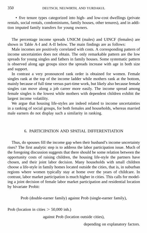
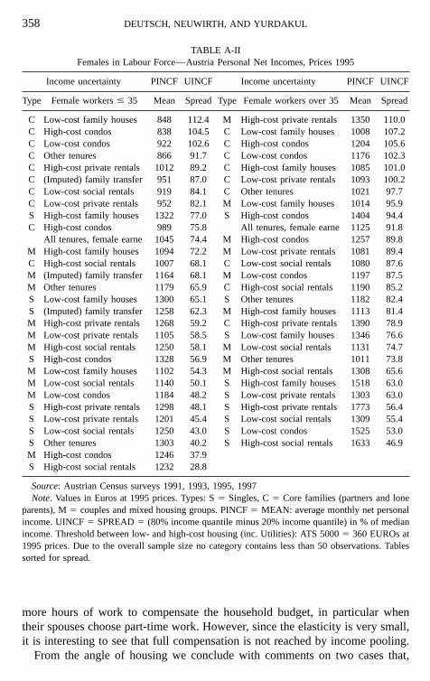
The percentage income spreads UNICM (males) and UINCF (females) areshown in Table A-I and A-II below. The main findings are as follows:
Male incomes are positively correlated with costs. A corresponding pattern ofincome uncertainties does not obtain. The only remarkable pattern are the lowspreads for young singles and fathers in family houses. Some systematic patternis observed along age groups since the spreads increase with age in both sizeand support.
In contrast a very pronounced rank order is obtained for women. Femalesingles rank at the top of the income ladder while mothers rank at the bottom,mainly because of full time versus part-time work, but likely also because femalesingles can move along a job career more easily. The income spread amongfemale singles is the lowest while mothers with dependent children exhibit thelargest income volatility.
We argue that housing life-styles are indeed related to income uncertaintiesin a ranking of social groups, for both females and households, whereas marriedmale earners do not display such a similarity in ranking.
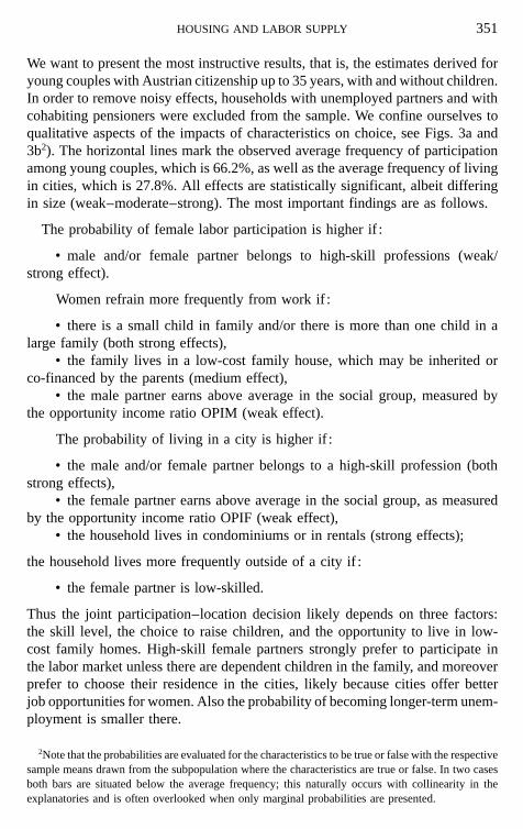
6. PARTICIPATION AND SPATIAL DIFFERENTIATION
Thus, do spouses fill the income gap when their husband’s income uncertaintyrises? The first analytic step is to address the labor participation issue. Much ofthe foregoing discussion suggests that there should be some relation between theopportunity costs of raising children, the housing life-style the partners havechosen, and their joint labor decision. Many households with small childrenchoose a life-style in family homes located outside the cities, that is, in suburbanregions where women typically stay at home over the years of childcare. Incontrast, labor market participation is much higher in cities. This calls for model-ing a joint decision of female labor market participation and residential locationby bivariate Probit:
Prob (double-earner family) against Prob (single-earner family),
Prob (location in cities . 50,000 inh.)
against Prob (location outside cities),
depending on explanatory factors.
HOUSING AND LABOR SUPPLY 351
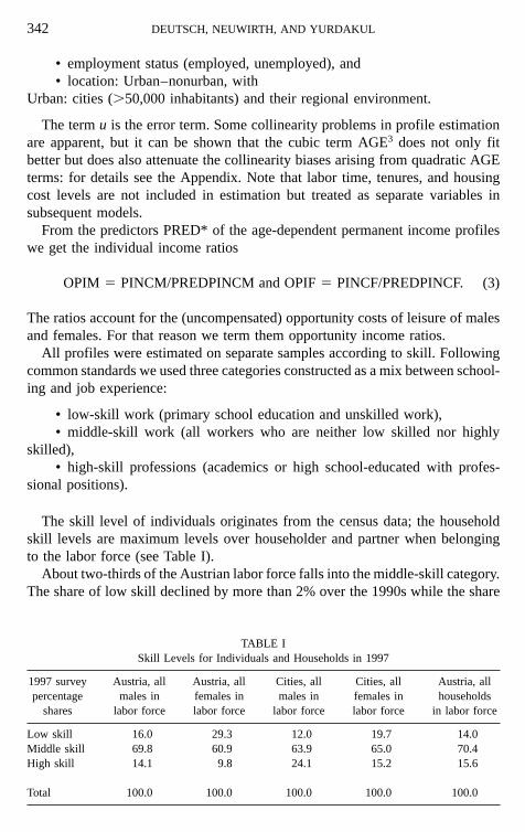
We want to present the most instructive results, that is, the estimates derived foryoung couples with Austrian citizenship up to 35 years, with and without children.In order to remove noisy effects, households with unemployed partners and withcohabiting pensioners were excluded from the sample. We confine ourselves toqualitative aspects of the impacts of characteristics on choice, see Figs. 3a and3b2). The horizontal lines mark the observed average frequency of participationamong young couples, which is 66.2%, as well as the average frequency of livingin cities, which is 27.8%. All effects are statistically significant, albeit differingin size (weak–moderate–strong). The most important findings are as follows.
The probability of female labor participation is higher if :
• male and/or female partner belongs to high-skill professions (weak/strong effect).
Women refrain more frequently from work if :
• there is a small child in family and/or there is more than one child in alarge family (both strong effects),
• the family lives in a low-cost family house, which may be inherited orco-financed by the parents (medium effect),
• the male partner earns above average in the social group, measured bythe opportunity income ratio OPIM (weak effect).
The probability of living in a city is higher if :
• the male and/or female partner belongs to a high-skill profession (bothstrong effects),
• the female partner earns above average in the social group, as measuredby the opportunity income ratio OPIF (weak effect),
• the household lives in condominiums or in rentals (strong effects);
the household lives more frequently outside of a city if :
• the female partner is low-skilled.
Thus the joint participation–location decision likely depends on three factors:the skill level, the choice to raise children, and the opportunity to live in low-cost family homes. High-skill female partners strongly prefer to participate inthe labor market unless there are dependent children in the family, and moreoverprefer to choose their residence in the cities, likely because cities offer betterjob opportunities for women. Also the probability of becoming longer-term unem-ployment is smaller there.
2Note that the probabilities are evaluated for the characteristics to be true or false with the respectivesample means drawn from the subpopulation where the characteristics are true or false. In two casesboth bars are situated below the average frequency; this naturally occurs with collinearity in theexplanatories and is often overlooked when only marginal probabilities are presented.

352 DEUTSCH, NEUWIRTH, AND YURDAKUL
FIG. 3. (a) Simulation of joint partner decisions: Female job participation. Bivariate probitestimates, couples in MZ-surveys 1991–1997. (b) Simulation of joint partner decisions: Location incities. Bivariate probit estimates from couples, MZ-surveys 1991–1997.

HOUSING AND LABOR SUPPLY 353
Parallel to the bivariate model we evaluated binomial probit models of femaleparticipation over all family compositions and age groups, i.e., over the agegroups up to 35 and over 35 years. Since the labor participation estimates wereclose to bivariate modeling, we used the inverse Mills ratios obtained frombinomial estimation as explanatories for the subsequent joint labor supply models.
7. WORK AND RISK SHARING IN EMPLOYED PARTNERSHIPS
This section offers a statistical model that corroborates the hypothesis raisedin Section 2. The starting point is the mating problem over skill levels, whichattracted considerable attention in the literature. There is a priori no reasonwhy labor supply effects should be independent of the combined skill levels inpartnerships. From the selected sample, Table IV lists the mating shares in theAustrian population of employed partnerships. Almost one-half of all partnershipsfall in the mating category M–M. Mating of lower skill women with higher skillmen is more likely than conversely, but mating of L–H or H–L is rare. Weexcluded the latter from consideration. There remain seven categories each ofwhich is estimated by the simultaneous equation system:
LHM 5 CONST1 1 a1*LHF 1 b1*LOPIM 1 c1*LOPIF
1 p 1*UINCM 1 q1*UINCF 1 Xu1 1 u1, (4)
LHF 5 CONST2 1 a2*LHM 1 b2*LOPIM 1 c2*LOPIF
1 p 2*UINCM 1 q2*UINCF 1 Xu2 1 m*IMR 1 u2.
The endogenous variables are male and female log weekly work hours LHMand LHF. The explanatories are used as instruments. These are the male andfemale opportunity log income ratios LOPIM and LOPIF, the income uncertaintypercentages UINCM and UINCF, and the remaining explanatories summarized
TABLE IVPercentage Shares of Skill Mating
Female workers employedMale workers
employed L: low skill M: middle skill H: high skill Row total
L: low skill 8.4 5.8 0.3 14.5M: middle skill 22.5 47.3 3.5 73.4H: high skill 0.6 6.3 5.2 12.1
Column total 31.5 59.4 9.0 100.0
Note. Total of employed partnerships 5 100%. Data drawn from weighted sample means.
354 DEUTSCH, NEUWIRTH, AND YURDAKUL
in the matrix X. It contains dummies for locational choice in cities and sectorsof employment, where services are chosen as sector of reference. For women,the matrix X includes also the inverse Mills ratios IMR, which are obtained fromthe model of female labor participation choice.
The system is estimated by 3SLS from survey data restricted to employedpartnerships from 1991 to 1997 over the seven mating categories separately.Calendar year dummies are used but excluded from discussion here. A fullaccount of estimation is given in Table A.2.1 of the Appendix. Two remarks onestimation are essential.
The first remark refers to the maintained hypothesis that the income uncertaintyvariables UINCM and UINCF properly account the ranking of housing costs.As we have seen this holds true for spouses but much less for husbands. Sincethe family status categories entered the calculation of these variables we excludedfamily characteristics from the explanatories in X. If labor supply is affected bydependent children this fact should show up in significant estimates for UINCMand UINCF.
The second remark refers to the opportunity income ratios LOPIM and LOPIF.They measure the individual incomes relative to their permanent component ina social group. Thus, even if the opportunity income variables are derived frominstrumental estimation of income profiles, they nevertheless include the numberof hours deviating from the work hours explained by the profile instruments.Therefore the wage income elasticities a1 and a2 w.r.t. work hours cannot beinterpreted as elasticities of work effort. A solution to the problem is discussedin the Appendix, see the remarks on estimation, yielding the so-called “modifiedreduced form coefficients,” which measure:
• the relative change of work hours DHM and DHF w.r.t. relative changesin hourly wages DWM and DWF;
• the relative change of hours of work DHM and DHF w.r.t. the deviationsDUINC and DUINCF of the income uncertainties from their group means.
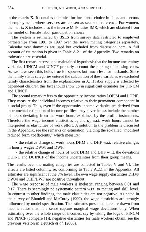
The results over the mating categories are collected in Tables V and VI. Theeffects are listed columnwise, conforming to Table A.2.1 in the Appendix. Allestimates are significant at the 5% level. The own wage supply elasticities DHM/DWM and DHF/DWF are positive throughout.
The wage response of male workers is inelastic, ranging between 0.01 and0.17. There is seemingly no systematic pattern w.r.t. to mating and skill level.In contrast to other findings, the male elasticities are not negative. As noted inthe survey of Blundell and MaCurdy (1999), the wage elasticities are stronglyinfluenced by model specification. The estimates presented here are drawn fromincome ratios that in a sense capture marginal wage deviations only. Whenestimating over the whole range of incomes, say by taking the logs of PINCMand PINCF (compare (1)), negative elasticities for male workers obtain, see theprevious version in Deutsch et al. (2000).
HOUSING AND LABOR SUPPLY 355
TABLE VWage Elasticities of Labor Supply, Employed Partnerships
Modified reduced formcoefficients Skill level of female partner
Low Middle HighExplanatory Skill level of
variable male partner DHM DHF DHM DHF DHM DHF
DWM Low 0.11 20.16 0.10 20.13DWF 20.01 0.97 0.00 0.60DWM Middle 0.01 20.19 0.03 20.10 0.10 0.00DWF 0.01 1.00 0.00 0.63 0.00 0.30DWM High 0.13 0.09 0.17 0.00DWF 0.00 0.50 0.00 0.46
The wage responses of female workers are somewhat more elastic, conformingto conventional wisdom, compare Blundell and Walker (1982) and Killingsworth(1983). Note also that the female own wage elasticities significantly decline withhigher skill levels. While lower skill women exhibit elastic responses in the rangeof 1.0, the own wage elasticity of highly skilled women is less than one-half.
By looking at the own wage elasticities columnwise it can be seen that theresponses of female workers of a given skill are only little affected by the skilllevel of their husbands. However there are negative cross-wage elasticities runningfrom male wages to the work effort response of spouses. Wage increases of low-and middle-skilled husbands permit their spouses to reduce their work effortslightly. Since family homes are strongly represented in these mating groups,
TABLE VIWork Hours and Income Uncertainty, Employed Partnerships
Modified reduced formcoefficients Skill level of female partner
Low Middle HighExplanatory Skill level of
variable male partner DHM DHF DHM DHF DHM DHF
DUINCM Low 0.00 0.00 0.10 20.13DUINCF 0.04 20.23 0.00 20.25(Group means) (56.1) (91.1) (54.4) (85.4)DUINCM Middle 0.00 0.00 0.00 0.25 0.00 0.00DUINCF 0.01 20.45 0.04 20.36 0.04 0.00(Group means) (56.0) (90.8) (55.3) (87.2) (56.0) (88.2)DUINCM High 0.00 0.00 0.00 0.00DUINCF 0.04 20.19 0.00 20.19(Group means) (58.1) (87.7) (59.5) (91.2)
356 DEUTSCH, NEUWIRTH, AND YURDAKUL
this supports the previous findings about household income pooling from theangle of housing life-styles, compare Section 4; in this sense, income poolingappears as a “middle class” phenomenon.
Indeed, for high skills the estimates reveal some different behavior. Wageincreases of high-skill husbands exert a slightly positive effect on middle-skillspouses. A possible reason is that higher incomes of male partners permit higherbudgets for organizing the household so that women can participate more activelyin the labor market. This interpretation is supported by the zero cross-wageelasticities among high-skill female partners; due to higher incomes they canprobably act more independently.
Most importantly, from the reduced form we obtain a substantial amplifiereffect. The structural elasticities obtained for the system (4) reappear in TableV magnified by factors between 1.5 and 2. Most part of that amplification resultsfrom income pooling within partnerships; for a simple proof see the Appendix.
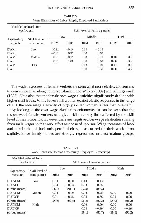
Now we turn to the responses of work hours to changes in income uncertaintiesUINCM and UINCF. The idea is that the income spread in a social group increasesby 1% over its initial size, which is given in the rows “group means,” see TableVI. The elasticities measure how individual work hours likely react in sucha situation.
Firstly, changing income uncertainties faced by husbands leaves their individualwork effort unaffected up to random responses. Almost alll male coefficientsw.r.t. DUINCM are zero. Since the rank order of male income spreads in TableA-I is only weakly correlated with the affordability of life-styles, some gender-specific differences in attitudes toward income uncertainty may answer why theissue of household income uncertainty on tenure choice remained inconclusive,compare Robst et al. (1999).
Instead there is some effect across genders: income uncertainties faced by low-and middle-skill males do influence female work effort albeit the sign is notuniform. In the mating category L–M there is a sort of negative risk synergy: ifhusbands are faced with greater uncertainty, women will reduce their work effort.Since the size of that effect is small we abstain from speculating about possiblereasons. A much larger effect is observed for the category M–M, which coversno less than 47% of all partnerships. Here we observe a marked risk shiftingeffect from men to women: a 10% increase in male income uncertainty yields aconsiderable 2.5% increase of female work hours. For an average female worktime of 34 h per week this amounts to almost one hour per week. The interpretationfollows the lines of risk pooling in the middle class.
The most systematic effects on female work hours are observed when femaleincome uncertainty increases itself. In six out of seven cases the response issignificant and negative. In the middle class it is 20.4 in magnitude. Lookingat the rank order of income spreads in Table A-II we can deduce that much ofthis result arises from motherhood. With dependent children in the householdthe impact amounts to 3 work hours less per week. This result is consistent with
HOUSING AND LABOR SUPPLY 357
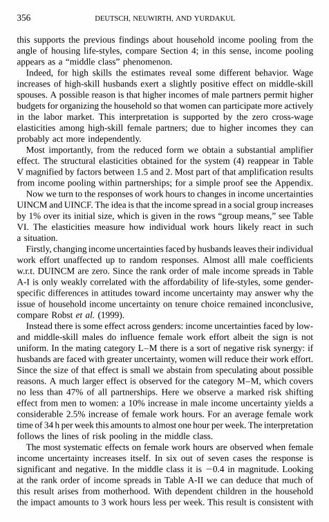
TABLE A-IMales in Labor Force—Austria: Personal Net Incomes, 1995 Prices
Income uncertainty PINCM UINCM Income uncertainty PINCM UINCM
Type Male workers # 35 Mean Spread Type Male workers over 35 Mean Spread
M High-cost condos 1534 69.2 M High-cost private rentals 2205 115.0C High-cost rentals 1695 64.7 M High-cost social rentals 1959 80.0C High-cost social rentals 1700 59.3 C High-cost private rentals 2251 79.9S Low-cost condos 1536 57.0 S High-cost condos 1963 78.5M High-cost family houses 1495 56.4 C High-cost social rentals 1973 72.4S High-cost private rentals 1480 55.6 S Low-cost family houses 1565 70.1C (Imputed) family transfer 1522 54.8 S Other tenures 1514 68.6M Low-cost condos 1571 54.7 C Low-cost condos 1986 67.0S Low-cost private rentals 1412 53.4 M High-cost condos 2106 66.9C High-cost condos 1724 51.3 C Low-cost private rentals 1716 66.1
All tenures, male earners 1514 51.1 S High-cost social rentals 1853 65.5C High-cost family houses 1615 50.1 All tenures, male earners 1598 65.3S Low-cost social rentals 1356 49.7 S Low-cost condos 1813 64.5S Other tenures 1325 49.6 C High-cost condos 2018 63.7C Other tenures 1516 48.7 S High-cost family houses 1640 61.3M High-cost social rentals 1590 48.4 S Low-cost private rentals 1525 61.3M Low-cost family houses 1424 48.2 M High-cost family houses 1744 60.9M Low-cost social rentals 1395 47.3 M Low-cost condos 1722 60.2C Low-cost family houses 1512 46.3 C Low-cost family houses 1734 60.0S High-cost condos 1643 45.7 C High-cost family houses 1791 59.4C Low-cost condos 1639 42.9 M Low-cost private rentals 1669 59.0C Low-cost private rentals 1526 42.8 S High-cost private rentals 2009 58.5S (Imputed) family transfer 1345 42.8 C Other tenures 1757 58.4M Low-cost private rentals 1429 42.7 M Low-cost family houses 1579 55.9C Low-cost social rentals 1520 41.9 M Low-cost social rentals 1589 55.5M Other tenures 1467 41.5 C Low-cost social rentals 1688 53.9S High-cost family houses 1385 40.0 S Low-cost social rentals 1479 51.1M (Imputed) family transfer 1384 36.3 M Other tenures 1572 45.8S High-cost social rentals 1552 34.6M High-cost private rentals 1568 34.5S Low-cost family houses 1299 31.9
Source: Austrian Census surveys 1991, 1993, 1995, 1997.Note. Values in Euros at 1995 prices. Types: S 5 Singles, C 5 Core families (partners and lone
parents), M 5 couples and mixed housing groups. PINCM 5 MEAN: average monthly net personalincome. UNICM 5 SPREAD 5 (80% income quantile minus 20% income quantile) in % of medianincome. Threshold between low- and high-cost housing (incl. Utilities): ATS 5000 5 360 EUROsat 1995 prices. Due to the overall sample size no category contains less than 50 observations. Tablessorted for Spread.
common sense because we know that mothers like to withdraw to part-time workof under 30 h per week.
In the categories of middle-skill husbands, increasing income uncertainty ofspouses raises male work effort slightly: The husbands tend to supply slightly
358 DEUTSCH, NEUWIRTH, AND YURDAKUL
TABLE A-IIFemales in Labour Force—Austria Personal Net Incomes, Prices 1995
Income uncertainty PINCF UINCF Income uncertainty PINCF UINCF
Type Female workers # 35 Mean Spread Type Female workers over 35 Mean Spread
C Low-cost family houses 848 112.4 M High-cost private rentals 1350 110.0C High-cost condos 838 104.5 C Low-cost family houses 1008 107.2C Low-cost condos 922 102.6 C High-cost condos 1204 105.6C Other tenures 866 91.7 C Low-cost condos 1176 102.3C High-cost private rentals 1012 89.2 C High-cost family houses 1085 101.0C (Imputed) family transfer 951 87.0 C Low-cost private rentals 1093 100.2C Low-cost social rentals 919 84.1 C Other tenures 1021 97.7C Low-cost private rentals 952 82.1 M Low-cost family houses 1014 95.9S High-cost family houses 1322 77.0 S High-cost condos 1404 94.4C High-cost condos 989 75.8 All tenures, female earne 1125 91.8
All tenures, female earne 1045 74.4 M High-cost condos 1257 89.8M High-cost family houses 1094 72.2 M Low-cost private rentals 1081 89.4C High-cost social rentals 1007 68.1 C Low-cost social rentals 1080 87.6M (Imputed) family transfer 1164 68.1 M Low-cost condos 1197 87.5M Other tenures 1179 65.9 C High-cost social rentals 1190 85.2S Low-cost family houses 1300 65.1 S Other tenures 1182 82.4S (Imputed) family transfer 1258 62.3 M High-cost family houses 1113 81.4M High-cost private rentals 1268 59.2 C High-cost private rentals 1390 78.9M Low-cost private rentals 1105 58.5 S Low-cost family houses 1346 76.6M High-cost social rentals 1250 58.1 M Low-cost social rentals 1131 74.7S High-cost condos 1328 56.9 M Other tenures 1011 73.8M Low-cost family houses 1102 54.3 M High-cost social rentals 1308 65.6M Low-cost social rentals 1140 50.1 S High-cost family houses 1518 63.0M Low-cost condos 1184 48.2 S Low-cost private rentals 1303 63.0S High-cost private rentals 1298 48.1 S High-cost private rentals 1773 56.4S Low-cost private rentals 1201 45.4 S Low-cost social rentals 1309 55.4S Low-cost social rentals 1250 43.0 S Low-cost condos 1525 53.0S Other tenures 1303 40.2 S High-cost social rentals 1633 46.9M High-cost condos 1246 37.9S High-cost social rentals 1232 28.8
Source: Austrian Census surveys 1991, 1993, 1995, 1997Note. Values in Euros at 1995 prices. Types: S 5 Singles, C 5 Core families (partners and lone
parents), M 5 couples and mixed housing groups. PINCF 5 MEAN: average monthly net personalincome. UINCF 5 SPREAD 5 (80% income quantile minus 20% income quantile) in % of medianincome. Threshold between low- and high-cost housing (inc. Utilities): ATS 5000 5 360 EUROs at1995 prices. Due to the overall sample size no category contains less than 50 observations. Tablessorted for spread.
more hours of work to compensate the household budget, in particular whentheir spouses choose part-time work. However, since the elasticity is very small,it is interesting to see that full compensation is not reached by income pooling.
From the angle of housing we conclude with comments on two cases that,
HOUSING AND LABOR SUPPLY 359
according to the estimates, deviate from middle-class behavior. Much of whatfollows is argued on similar lines as that in Costa and Kahn (2000).
The first case is the low-skill mating category L–L, which contributes 8.4%to all employed partnerships. Within that category, more than 60% of all house-holds live in smaller communities while 28% are found in cities with over 50,000inhabitants. Regarding tenures some 43% of all low-skill households own afamily home, for the most part located in smaller communities. The share oflow-skill owners in cities is negligible; most low-skill city inhabitants are privateor social renters. From Table V we have seen that the own wage elasticities inthe low-skill category are positive and elastic for female workers. Thus we cannotinfer about possible hour restrictions from the labor demand side. Althoughthe outcome is highly relevant for spatial differentiation: after many years ofsuburbanization there is now some self-enforcing trend to move back into metro-politan areas. Since lower-skill households react elastically to wage signals theywill likely move to a search for better job opportunities. If higher skills get rarein the countryside the lower-skill population sitting there may likely be facedwith higher risks of income and unemployment.
The second case is the mating categories with high-skill spouses. Among themating groups with high-skills income pooling appears less likely. The matingcategory H–H shows no risk sharing at all; high-skill partners seemingly actindependently from each other. From the bivariate Probit model we have alreadyseen that high-skill women prefer to live in city areas. The major motives arejob opportunities, better care services for dependent children, and certainly alsovarious amenities of urban life. This makes it possible to speculate that highlyeducated women exercise an option for city locations while middle-class couplesof comparable skills wish to live in family homes outside the city limits.
8. SINGLES
Single-person households deserve more attention than often attributed in theliterature. Certainly the limited statistical information about risk perception amongsingles makes econometric model building difficult. Additional barriers stemfrom the definition of singles because surveys—among them the Austrian cen-sus—do not reveal whether (mostly male) divorced singles pay or care fordependent children outside the own household. Moreover, in the larger citiessome 40–45% of all adults under 50 years are singles but only a minority liveas solitaires; most singles share stable or fluctuating partnerships in separatedhouseholds. Some degree of income pooling is therefore likely but impossibleto infer from household data.
Despite these possibly severe restrictions we try to characterize the labor supplybehavior of singles based on OLS equations of type (1) over separate skill levels.
360 DEUTSCH, NEUWIRTH, AND YURDAKUL
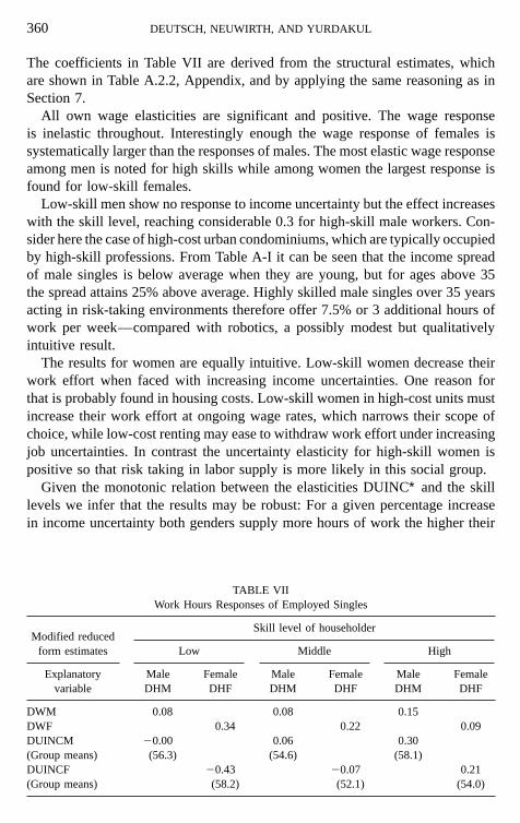
The coefficients in Table VII are derived from the structural estimates, whichare shown in Table A.2.2, Appendix, and by applying the same reasoning as inSection 7.
All own wage elasticities are significant and positive. The wage responseis inelastic throughout. Interestingly enough the wage response of females issystematically larger than the responses of males. The most elastic wage responseamong men is noted for high skills while among women the largest response isfound for low-skill females.
Low-skill men show no response to income uncertainty but the effect increaseswith the skill level, reaching considerable 0.3 for high-skill male workers. Con-sider here the case of high-cost urban condominiums, which are typically occupiedby high-skill professions. From Table A-I it can be seen that the income spreadof male singles is below average when they are young, but for ages above 35the spread attains 25% above average. Highly skilled male singles over 35 yearsacting in risk-taking environments therefore offer 7.5% or 3 additional hours ofwork per week—compared with robotics, a possibly modest but qualitativelyintuitive result.
The results for women are equally intuitive. Low-skill women decrease theirwork effort when faced with increasing income uncertainties. One reason forthat is probably found in housing costs. Low-skill women in high-cost units mustincrease their work effort at ongoing wage rates, which narrows their scope ofchoice, while low-cost renting may ease to withdraw work effort under increasingjob uncertainties. In contrast the uncertainty elasticity for high-skill women ispositive so that risk taking in labor supply is more likely in this social group.
Given the monotonic relation between the elasticities DUINC∗ and the skilllevels we infer that the results may be robust: For a given percentage increasein income uncertainty both genders supply more hours of work the higher their
TABLE VIIWork Hours Responses of Employed Singles
Skill level of householderModified reduced
form estimates Low Middle High
Explanatory Male Female Male Female Male Femalevariable DHM DHF DHM DHF DHM DHF
DWM 0.08 0.08 0.15DWF 0.34 0.22 0.09DUINCM 20.00 0.06 0.30(Group means) (56.3) (54.6) (58.1)DUINCF 20.43 20.07 0.21(Group means) (58.2) (52.1) (54.0)
HOUSING AND LABOR SUPPLY 361
skill level. In other words, low-skill singles appear rather risk averse whilehigh-skill singles can take more risk to afford their preferred life-styles underuncertainty.
9. CONCLUSIONS
This study has offered empirical evidence on housing life-styles and laborchoice. The main objective of this paper was to condense available evidence intoa hypothesis about the impact of life-style-related income uncertainties on hoursof work supplied. Up to certain limits the scale of income uncertainties seemsto explain work effort in partnerships and among singles. In particular, femalelabor market participation and the choice of hours is controlled by partners wagesand life-style costs, but the effects get weaker with rising female skill levels.High-skill female workers do not refrain from full-time work unless there aresmall children in the family. The outcome points to possible conflicts in locationalchoice when women prefer city areas while men tend to family homes in suburbanregions. The process of skill upgrading may get additional momentum whencities succeed in attracting a highly skilled female labor force.
REFERENCES
Ball, M. (2000). Annual Review of European Housing Markets. European Society of CharteredSurveyors, Rics.
Blundell, R., and Walker, I. (1982). “Modelling the joint determination of household labour suppliesand commodity demands,” Econ. J. 92, 351–364.
Blundell, R., and MaCurdy, Th. (1999). “Labor Supply—A review of alternative approaches,” inHandbook of Labor Economics (O. Ashenfelter and D. Card, Eds.), Vol. 3A, Chap. 25, pp.1559–1695. Amsterdam: Elsevier.
Costa, D., and Kahn, M. (2000). “Power Couples: Changes in the Locational Choice of the CollegeEducated, 1940–1990,” Quart. J. Econ. 114, 1287–1312.
Deaton, A., and Muellbauer, J. (1980). Economics and Consumer Behaviour. Cambridge, UK: Cam-bridge Univ. Press.
Deutsch, E. (1997). “Indicators of Housing Finance and Intergenerational Wealth Transfers,” RealEstate Econ. 25, 131–174.
Erreygers, G., and Vandevelde, T. (1997). Is Inheritance Legitimate? Ethical and Economic Aspectsof Wealth Transfers. New York: Springer-Verlag.
Fortin, N. (1995). “Allocation Inflexibilities, Female Labor Supply, and Housing Asset Accumulation:Are Women Working to Pay the Mortgage?” J. Labor Econ. 13, 524–557.
Franz, W. (2000). “Real and monetary challenges to wage policy in Germany at the turn of themillenium: Technical progress, globalisation and European Monetary Union,” CES ifo Forum,Spring 12–14.
Gabriel, S., and Rosenthal, S. (1999). “Location and the effect of demographic traits on earnings.”Regional Sci. Urban Econ. 29, 445–461.

362 DEUTSCH, NEUWIRTH, AND YURDAKUL
Killingsworth, M. R. (1983). Labor Supply. Cambridge, UK: Cambridge Univ. Press.
Robst, J., Deitz, R., and McGoldrick, K. (1999). “Income variability, uncertainty and housing tenurechoice,” Regional Sci. Urban Econ. 29, 219–229.
van Ommeren, J., Rietveld, P., and Nijkamp, P. (1999). “Job Moving, Residential Moving, andCommuting: A Search Perspective,” J. Urban Econ. 46, 230–253.
Related Documents