Housewife, “Gold Miss,” and Equal: The Evolution of Educated Women’s Role in Asia and the U.S. Jisoo Hwang ∗ November 10, 2012 JOB MARKET PAPER Abstract The fraction of U.S. college graduate women who ever marry has increased rela- tive to less educated women since the mid-1970s. In contrast, college graduate women in developed Asian countries have had decreased rates of marriage, so much so that the term “Gold Misses” has been coined to describe them. This paper argues that the interaction of rapid economic growth in Asia combined with the intergenerational trans- mission of gender attitudes causes the “Gold Miss” phenomenon. Economic growth has increased the supply of college graduate women, but men’s preference for their wives’ household services has diminished less rapidly and is slowed by women’s role in their mothers’ generation. Using a dynamic model, I show that a large positive wage shock produces a greater mismatch between educated women and men in the marriage market than would gradual wage growth. I test the implications of the model using three data sets: the Japanese General Social Survey, the American Time Use Survey, and the U.S. Census and American Community Survey. Using the Japanese data, I find a positive relationship between a mother’s education (and employment) and her son’s gender attitudes. In the U.S., time spent on household chores among Asian women is inversely related to the female labor force participation rate in husband’s country of origin. Lastly, college graduate Korean and Japanese women in the U.S. have greater options in the marriage market. They are more likely to marry Americans than Korean and Japanese men do, and this gender gap is larger among the foreign born than the U.S. born. * Department of Economics, Harvard University ([email protected]) I am grateful to Alberto Alesina, Raj Chetty, Claudia Goldin, and Lawrence Katz for their guidance and feedback throughout this project. I would also like to thank Wenxin Du, John Friedman, Paola Giuliano, Edward Glaeser, Seok Ki Kim, Joana Naritomi, Claudia Olivetti, Amanda Pallais, Dana Rotz, L´ aszl´oS´ andor, Anitha Sivasankaran, and seminar participants at Harvard University for helpful comments and discussions. This project received financial support from the Lab for Economic Applications and Policy at Harvard University. All remaining errors are my own. 1

Welcome message from author
This document is posted to help you gain knowledge. Please leave a comment to let me know what you think about it! Share it to your friends and learn new things together.
Transcript
Housewife, “Gold Miss,” and Equal: The Evolution of
Educated Women’s Role in Asia and the U.S.
Jisoo Hwang∗
November 10, 2012
JOB MARKET PAPER
Abstract
The fraction of U.S. college graduate women who ever marry has increased rela-tive to less educated women since the mid-1970s. In contrast, college graduate womenin developed Asian countries have had decreased rates of marriage, so much so thatthe term “Gold Misses” has been coined to describe them. This paper argues that theinteraction of rapid economic growth in Asia combined with the intergenerational trans-mission of gender attitudes causes the “Gold Miss” phenomenon. Economic growthhas increased the supply of college graduate women, but men’s preference for theirwives’ household services has diminished less rapidly and is slowed by women’s role intheir mothers’ generation. Using a dynamic model, I show that a large positive wageshock produces a greater mismatch between educated women and men in the marriagemarket than would gradual wage growth. I test the implications of the model usingthree data sets: the Japanese General Social Survey, the American Time Use Survey,and the U.S. Census and American Community Survey. Using the Japanese data, I finda positive relationship between a mother’s education (and employment) and her son’sgender attitudes. In the U.S., time spent on household chores among Asian women isinversely related to the female labor force participation rate in husband’s country oforigin. Lastly, college graduate Korean and Japanese women in the U.S. have greateroptions in the marriage market. They are more likely to marry Americans than Koreanand Japanese men do, and this gender gap is larger among the foreign born than theU.S. born.
∗Department of Economics, Harvard University ([email protected])I am grateful to Alberto Alesina, Raj Chetty, Claudia Goldin, and Lawrence Katz for their guidance and
feedback throughout this project. I would also like to thank Wenxin Du, John Friedman, Paola Giuliano,Edward Glaeser, Seok Ki Kim, Joana Naritomi, Claudia Olivetti, Amanda Pallais, Dana Rotz, Laszlo Sandor,Anitha Sivasankaran, and seminar participants at Harvard University for helpful comments and discussions.This project received financial support from the Lab for Economic Applications and Policy at HarvardUniversity. All remaining errors are my own.
1
1 Introduction
Marriage rates have decreased among women in Japan, South Korea (hereafter Korea),
Taiwan, Singapore, and Hong Kong during the past several decades. As covered in a recent
article in The Economist, “The Asian avoidance of marriage is new, and striking. ... In
South Korea, young men complain that women are on marriage strike.”1 The majority of
women on this “marriage strike” are highly educated, four-year college graduates. Koreans
call this growing group of educated single women “Gold Misses.”2
Later marriages are common among the educated worldwide. What is striking about the
phenomenon in Asia, however, is that Gold Misses are not merely delaying marriage. Rather,
they are remaining single and at a much higher cost than in the West. Cohabitation is rare
and out-of-wedlock childbirths make up less than 2 percent of total childbirths in Korea
and Japan.3 Moreover, the gap in marriage rates between college graduate and non-college
graduate women has not diminished in Asia—it has grown. In the U.S., in contrast, the gap
narrowed and reversed in the mid-1970s.4
Why are there Gold Misses and why are they increasing in developed Asia? This paper
argues that the interaction of Asia’s rapid economic growth combined with the intergener-
ational transmission of gender attitudes causes the Gold Miss phenomenon. Wage growth
creates incentives for more women to become educated and to participate in the labor mar-
ket. However, gender norms do not shift at once; they are passed from one generation to the
next. Men are still accustomed to women being housewives as in their mothers’ generation
and have preference for wives’ household services. Thus, some educated women choose to
remain single rather than marry “traditional” men.
The story sketched above emerges from a simple dynamic model of intergenerational
transmission of gender attitudes, in which the fraction of men with preference for wives’
household time decreases with the fraction of educated women in the previous generation.
Women’s education, marriage, and household time allocation decisions are functions of the
endogenously evolving preferences within the male population.5 The model predicts that
Gold Misses are more likely to arise in economies that experience rapid, rather than gradual,
1The Economist, “The flight from marriage,” August 20th 2011.2Terms have been coined in each region to refer to this group—in Korean Gold Miss (because they are
“old misses” but highly educated and financially independent), in Japanese Hanako-zoku (literally “Hanakotribe,” named after the readers of the consumer magazine Hanako, which targets young single women) orWagamama (translated as “single parasites” because most unmarried adults live with their parents), andin Chinese Shengu (translated as “leftover women”). Among these, I choose to use the term Gold Missthroughout this paper.
3Korea and Japan are ranked the two lowest among OECD countries in out-of-wedlock childbirths. 38percent of births are out-of-wedlock in the U.S. (OECD Family Database, 2011)
4See Figure 4. For references on the trends of U.S. college graduate women’s marriage and fertility, seefor example, Kalmijn (1991), Goldin (2004), Schwartz and Mare (2005), Stevenson and Wolfers (2007) andShang and Weinberg (2012).
5c.f., Fernandez, Fogli and Olivetti (2004).
2
growth in women’s wages.
To empirically evaluate this hypothesis, I use three different datasets. First, I use the
Japanese General Social Survey to explore the gender attitudes and marriage patterns of
Japanese men. Second, I use the American Time Use Survey to study time allocation at
home among married couples in the U.S. by their country of origin and generation since
migrating to the U.S. Lastly, I use the U.S. census data to analyze marriage patterns of men
and women from two major Gold Miss countries—Korea and Japan.
I find evidence consistent with the implications of my model. First, men’s gender attitudes
are affected by the economic status of women in their parents’ generation. Men in Japan
who had working or college graduate mothers during childhood have more egalitarian views
regarding gender roles, and are more likely to have working wives. Among U.S. immigrants
from countries with low female labor force participation (LFP) rates, U.S. born men spend
about 1 hour per week more on housework relative to foreign born men, and reduce their
wives’ time spent on housework by 4 hours per week.
Second, women marry “less traditional” men (rather than “traditional”) when they are
available. In Japan, the probability that a college graduate man ever marries is positively
correlated with his mother’s LFP. Among Koreans and Japanese residing in the U.S., foreign
born women are 20 percentage points more likely than their male peers to marry a non-
Korean or non-Japanese. I exploit regional variation in the composition of male population
to show that Korean and Japanese women are more likely to marry out of their ethnic group
when the foreign born share is higher among Korean and Japanese men.
Third, the increase in Gold Misses is less severe when the fraction of “less traditional”
men in the marriage market is larger. In contrast to Korea and Japan, I find that college
graduate Korean and Japanese women in the U.S. are as likely to be married as the non-
college graduates.
The results indicate that educated women’s marriage prospects are better when the
generation gap in women’s educational attainment (and LFP) is smaller. This offers new
insight into the forces underlying the evolution of educated women’s role. Previous studies
have focused on the supply-side determinants such as the introduction of the pill, the opening
up of co-ed universities, and the advancements in household appliances technology.6 These
changes enabled the supply of educated and working women to increase in the marriage
market. However, this paper demonstrates that an equally important determinant is the
demand-side—whether men want educated and working wives who outsource housework—
and thereby shows how women’s role may not transition smoothly from housewife to equal
even with economic growth.7 I also add to the line of research on cultural norms by providing
6See for example, Goldin and Katz (2002), Goldin and Katz (2011), Greenwood, Seshadri and Yorukoglu(2005), and Greenwood and Guner (2009).
7Feyrer, Sacerdote and Stern (2008) share similar intuitions, although they do not present a formal model.Looking at cross-country differences in fertility rates, they argue that countries where women’s household
3

an example of how rigid gender roles may weaken in response to changes in women’s relative
wages, and research on the assimilation of immigrants by explaining why there may be
significant gender gaps in marital assimilation.8
The remainder of the paper is organized as follows. Section 2 provides an overview of the
Gold Miss phenomenon with statistics from developed Asian countries. Section 3 presents
the dynamic model. Section 4 lays out the empirical results. Section 5 concludes.
2 Background: The Gold Miss Phenomenon in Asia
Gold Miss (and analogous terms used in Asia, see footnote 2) colloquially means a never
married woman in her thirties or older who has received at least a four-year college education,
has her own career, and earns a higher-than-average yearly income. She is not just a “Miss,”
she is a rich one. In order to use one general standard for different countries, in this paper I
define Gold Miss as a four-year college graduate woman over age 35 who has never married.9
The Gold Miss phenomenon then refers to the increase in the share of college graduate
women who have never married relative to that of non-college graduate women.
The Gold Miss countries are the East Asian “tiger economies” that achieved economic
miracles over the past half-century. Figure 1 depicts the historical trend of GDP per capita
in Hong Kong, Japan, Korea, Singapore, and Taiwan in comparison to the U.S. and the
world average from 1900 to present. The growth trajectories of the Asian economies share
a common pattern—rapid economic development from the 1960s onward (with growth rates
in excess of 7 percent a year). The U.S. has had a higher GDP per capita than Asia since
the early 20th century and follows a more gradual growth path throughout.
Industrialization opened up (and benefited from) new opportunities for women. Accord-
ing to the United Nations statistics for 1985–2006 on labor force participation (LFP) rates of
women in the age group 25–34, the U.S. begins at around 70 percent. Rates in Japan, Korea,
and Singapore begin much lower (56.6 percent, 39.2 percent, and 58.3 percent, respectively).
The Asian rates then increased by more than 17 percentage points from 1985 to 2006; the
U.S. rates increased by 5 percentage points.
Educational attainment shows a similar pattern. There were virtually no college graduate
status lags behind their labor market opportunities experience the lowest fertility rates.8See for example, Giuliano (2007), Fernandez and Fogli (2009), Alesina and Giuliano (2010), Alesina,
Nunn and Guiliano (2011) for discussions on the persistence of family culture. Regarding assimilation profilesby gender, Blau and Kahn (2007) study Mexican immigrants in the U.S. and find dramatic assimilation inlabor supply for female immigrants.
9Age thirty-five is young enough to capture recent developments and old enough to distinguish between“marriage delayed” and “marriage forgone” among women in Asia. Despite the rise in women’s age at firstmarriage—29 in Japan and Korea, 28 in Taiwan, 30 in Hong Kong, and 28 in Singapore (Jones and Gubhaju(2009))—marriage rates fall starkly once women reach their late thirties. The age-specific marriage rate forbrides in age group 35–39 is only 12.2 (per thousand) in Korea and 9.2 (per thousand) in Japan (StatisticsKorea, 2010 and Vital Statistics of Japan, 2009). The peak is at ages 25–29 for brides in both countries.
4
women in East Asia before World War II. However, with economic growth and education
reforms, tertiary enrollments greatly increased.10 Figure 2 shows college enrollment rates
in Japan and Korea by sex. In Japan, although the college gender gap persists, women’s
college enrollment rates rose from near zero in 1955 to 41 percent in 2007. In Korea, women’s
enrollment rates increased from 20 percent to 55 percent in just 18 years and the college
gender gap has disappeared.
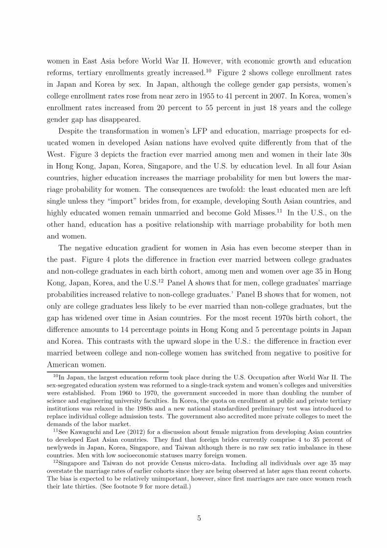
Despite the transformation in women’s LFP and education, marriage prospects for ed-
ucated women in developed Asian nations have evolved quite differently from that of the
West. Figure 3 depicts the fraction ever married among men and women in their late 30s
in Hong Kong, Japan, Korea, Singapore, and the U.S. by education level. In all four Asian
countries, higher education increases the marriage probability for men but lowers the mar-
riage probability for women. The consequences are twofold: the least educated men are left
single unless they “import” brides from, for example, developing South Asian countries, and
highly educated women remain unmarried and become Gold Misses.11 In the U.S., on the
other hand, education has a positive relationship with marriage probability for both men
and women.
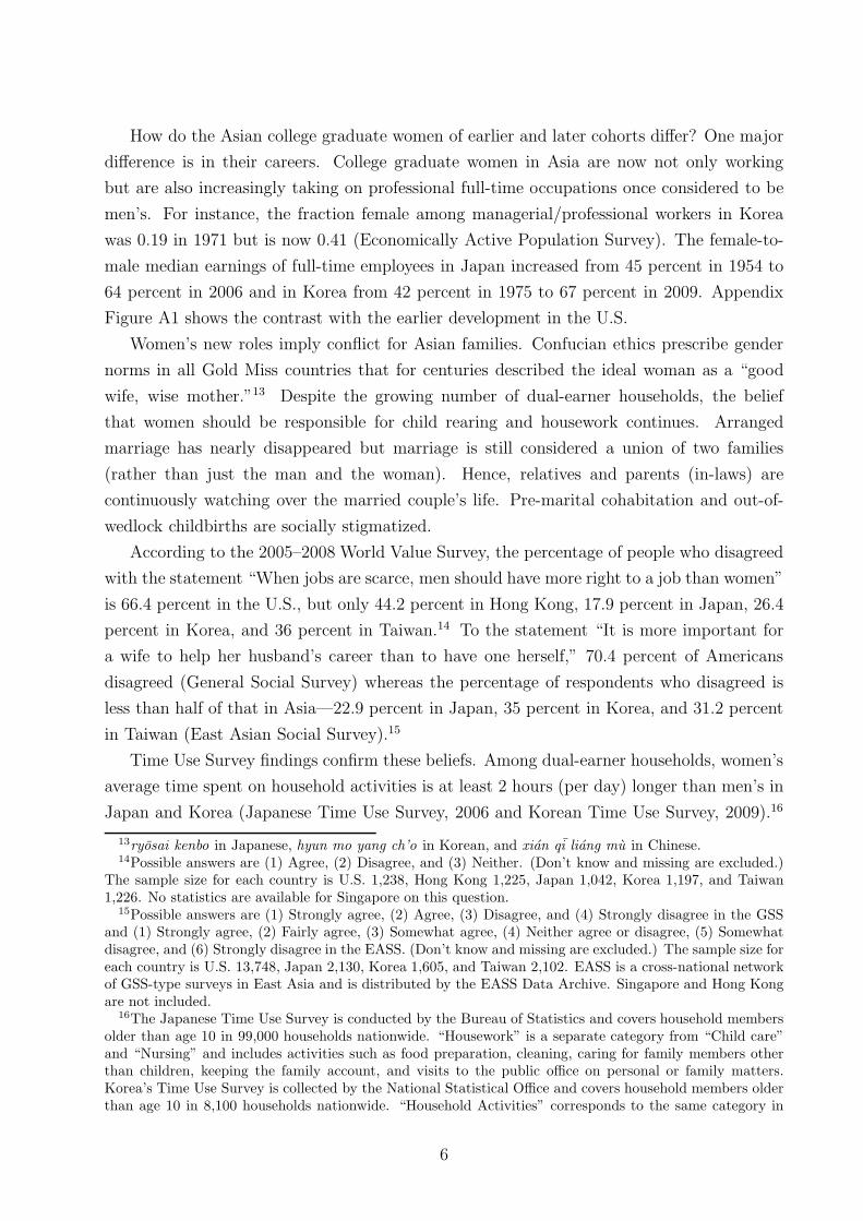
The negative education gradient for women in Asia has even become steeper than in
the past. Figure 4 plots the difference in fraction ever married between college graduates
and non-college graduates in each birth cohort, among men and women over age 35 in Hong
Kong, Japan, Korea, and the U.S.12 Panel A shows that for men, college graduates’ marriage
probabilities increased relative to non-college graduates.’ Panel B shows that for women, not
only are college graduates less likely to be ever married than non-college graduates, but the
gap has widened over time in Asian countries. For the most recent 1970s birth cohort, the
difference amounts to 14 percentage points in Hong Kong and 5 percentage points in Japan
and Korea. This contrasts with the upward slope in the U.S.: the difference in fraction ever
married between college and non-college women has switched from negative to positive for
American women.
10In Japan, the largest education reform took place during the U.S. Occupation after World War II. Thesex-segregated education system was reformed to a single-track system and women’s colleges and universitieswere established. From 1960 to 1970, the government succeeded in more than doubling the number ofscience and engineering university faculties. In Korea, the quota on enrollment at public and private tertiaryinstitutions was relaxed in the 1980s and a new national standardized preliminary test was introduced toreplace individual college admission tests. The government also accredited more private colleges to meet thedemands of the labor market.
11See Kawaguchi and Lee (2012) for a discussion about female migration from developing Asian countriesto developed East Asian countries. They find that foreign brides currently comprise 4 to 35 percent ofnewlyweds in Japan, Korea, Singapore, and Taiwan although there is no raw sex ratio imbalance in thesecountries. Men with low socioeconomic statuses marry foreign women.
12Singapore and Taiwan do not provide Census micro-data. Including all individuals over age 35 mayoverstate the marriage rates of earlier cohorts since they are being observed at later ages than recent cohorts.The bias is expected to be relatively unimportant, however, since first marriages are rare once women reachtheir late thirties. (See footnote 9 for more detail.)
5
How do the Asian college graduate women of earlier and later cohorts differ? One major
difference is in their careers. College graduate women in Asia are now not only working
but are also increasingly taking on professional full-time occupations once considered to be
men’s. For instance, the fraction female among managerial/professional workers in Korea
was 0.19 in 1971 but is now 0.41 (Economically Active Population Survey). The female-to-
male median earnings of full-time employees in Japan increased from 45 percent in 1954 to
64 percent in 2006 and in Korea from 42 percent in 1975 to 67 percent in 2009. Appendix
Figure A1 shows the contrast with the earlier development in the U.S.
Women’s new roles imply conflict for Asian families. Confucian ethics prescribe gender
norms in all Gold Miss countries that for centuries described the ideal woman as a “good
wife, wise mother.”13 Despite the growing number of dual-earner households, the belief
that women should be responsible for child rearing and housework continues. Arranged
marriage has nearly disappeared but marriage is still considered a union of two families
(rather than just the man and the woman). Hence, relatives and parents (in-laws) are
continuously watching over the married couple’s life. Pre-marital cohabitation and out-of-
wedlock childbirths are socially stigmatized.
According to the 2005–2008 World Value Survey, the percentage of people who disagreed
with the statement “When jobs are scarce, men should have more right to a job than women”
is 66.4 percent in the U.S., but only 44.2 percent in Hong Kong, 17.9 percent in Japan, 26.4
percent in Korea, and 36 percent in Taiwan.14 To the statement “It is more important for
a wife to help her husband’s career than to have one herself,” 70.4 percent of Americans
disagreed (General Social Survey) whereas the percentage of respondents who disagreed is
less than half of that in Asia—22.9 percent in Japan, 35 percent in Korea, and 31.2 percent
in Taiwan (East Asian Social Survey).15
Time Use Survey findings confirm these beliefs. Among dual-earner households, women’s
average time spent on household activities is at least 2 hours (per day) longer than men’s in
Japan and Korea (Japanese Time Use Survey, 2006 and Korean Time Use Survey, 2009).16
13ryosai kenbo in Japanese, hyun mo yang ch’o in Korean, and xian qi liang mu in Chinese.14Possible answers are (1) Agree, (2) Disagree, and (3) Neither. (Don’t know and missing are excluded.)
The sample size for each country is U.S. 1,238, Hong Kong 1,225, Japan 1,042, Korea 1,197, and Taiwan1,226. No statistics are available for Singapore on this question.
15Possible answers are (1) Strongly agree, (2) Agree, (3) Disagree, and (4) Strongly disagree in the GSSand (1) Strongly agree, (2) Fairly agree, (3) Somewhat agree, (4) Neither agree or disagree, (5) Somewhatdisagree, and (6) Strongly disagree in the EASS. (Don’t know and missing are excluded.) The sample size foreach country is U.S. 13,748, Japan 2,130, Korea 1,605, and Taiwan 2,102. EASS is a cross-national networkof GSS-type surveys in East Asia and is distributed by the EASS Data Archive. Singapore and Hong Kongare not included.
16The Japanese Time Use Survey is conducted by the Bureau of Statistics and covers household membersolder than age 10 in 99,000 households nationwide. “Housework” is a separate category from “Child care”and “Nursing” and includes activities such as food preparation, cleaning, caring for family members otherthan children, keeping the family account, and visits to the public office on personal or family matters.Korea’s Time Use Survey is collected by the National Statistical Office and covers household members olderthan age 10 in 8,100 households nationwide. “Household Activities” corresponds to the same category in
6
Gender gap exists in the U.S. as well, but the magnitude is much smaller—50 minutes per
day (American Time Use Survey, 2003–2011).
There is virtually no difference in household appliances technology between the Gold
Miss countries and other developed countries. The relative price of hiring a live-in domestic
worker in the U.S. and in East Asia is also comparable, at about 40 percent of the mean
wage of native college graduate women. In fact, the price is lower in Taiwan and Singapore,
and particularly lower in Hong Kong, than in the U.S.17
Thus, although the Gold Miss phenomenon may look similar with what occurred in the
U.S. and elsewhere when women first began to graduate from college, there are important
differences. In the early twentieth century, women could not easily have both family and
career with the (lack of) contraceptive methods, household appliances technology, market
substitutes for household production, and labor market opportunities (Goldin (2004)). As
surveyed in this section, women in developed Asia today do not face these conditions. Rather,
the constraints of marriage derive from traditional household roles families expect from the
wife and daughter-in-law.
3 Model of the Intergenerational Transmission of
Gender Attitudes and of Marriage
Building on the framework of Fernandez, Fogli and Olivetti (2004), I develop a simple dy-
namic model where women’s education, marriage, and labor force participation decisions
are functions of wages and the endogenously evolving types within the male population—
“traditional” and “modern.” I define a man as traditional if he has preference for his wife’s
household services and modern if he is willing to substitute wife’s housework with his own
or with market goods and services. The fraction of modern men increases with the fraction
of educated women in the previous generation.
When women’s wages rise, more women choose to stay single than marry traditional
husbands. The key distinguishing prediction of this model is the path dependency of the
Gold Miss phenomenon. Given that men initially hold traditional values, economies where
women’s wages increased rapidly are more likely to experience the Gold Miss phenomenon
the Bureau of Labor Statistics time use data. Activities such as housework, food and drink preparation andclean-up, interior maintenance, exterior maintenance, vehicle maintenance, and household management areincluded. It does not include time spent on caring for children or other family members.
17Hong Kong has a foreign domestic worker (FDW) program and the government sets the minimum wagefor these workers. According to Cortes and Pan (forthcoming), the minimum wage is more than four timeslower than high skilled women’s wage. Though limited, Taiwan and Singapore have similar programs; theFDW’s wage is about 30–40 percent of native college graduate women’s. Japan and Korea have stricterimmigration policies. The relative price of live-in domestic workers is nearly half of native college graduatewomen’s wage, as in the U.S. (See Huang, Yeoh and Rahman (2005) for more information on foreign domesticworkers.)
7
compared with economies where women’s wages increased gradually over time. In the rapid
case, a large discrepancy appears between the women’s roles when men were growing up and
women’s roles in their own cohort. As a result, there are not enough modern men for the
newly educated women to marry.18
I make the following assumptions for tractability. Women differ in their effort costs of
becoming educated and can choose to invest in education (“educated,” E) or not (“uned-
ucated,” U). If a woman invests in her education, she gets wage wE in the labor market,
which is higher than the wage she would get if uneducated, wU . wE is randomly drawn from
a distribution that varies exogenously over time. Men, on the other hand, are assumed to
have homogeneous skill level and earn wm in the labor market.19 Men differ in their cultural
upbringing: those who grew up around educated women develop less traditional gender atti-
tudes (“modern,” M) compared with those who grew up around housewives (“traditional,”
T ). All agents are rational and forward-looking.
The timing in the model is as follows. In the first period, women decide whether or not to
become educated. In the second period, men and women are randomly matched and decide
whether to get married or remain single. In the third period, men and women decide on
a time allocation between market activity and household production. Below I describe the
intergenerational dynamics and then solve for each stage of the decision-making process.
3.1 Intergenerational Dynamics
Gender attitudes (or more specifically, men’s preferences for wives’ household services) are
transmitted from mother to son. Assuming, as is reasonable for Asia, that only married
women have children, the fraction of modern men (λM) in cohort t then depends on the
fraction of married educated women in the previous cohort. The dynamics of the system are
thus given by:
λMt+1(λMt) = pEt(λMt)λEt(λMt) (1)
18Standard models of household production can also show that growth in women’s earning power reducesthe gain from marriage or that positive assortative mating becomes optimal as technology advances (Becker(1991)). However, they cannot explain why marriage patterns would evolve differently across similarlydeveloped countries. Intra-household models also face this limitation if bargaining power is a function ofonly wages. (See Chiappori and Donni (2011) for a survey of this literature.) Assuming that the sharing ruleis affected by other “distribution factors,” in which gender attitudes can be a component, is an option. Thedifference with my model would then be that the husband’s type affects the wife’s utility via consumption.
19If men also differed in their educational attainment and wages, there would be four categories of men,with the modern and educated being the most attractive husband and the traditional and uneducated beingthe least attractive. Figure 3 Panel A and Kawaguchi and Lee (2012) address this outcome. Since mypaper’s focus is on the Gold Misses, I do not add the education dimension to men. But the traditional anduneducated men not being able to marry is a by-product of the Gold Miss phenomenon, and can thus beexplained by the same mechanisms.
8
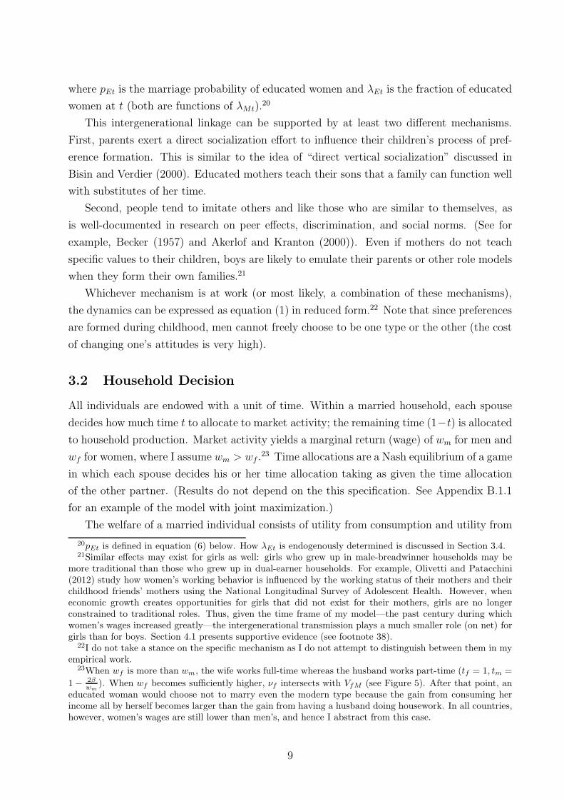
where pEt is the marriage probability of educated women and λEt is the fraction of educated
women at t (both are functions of λMt).20
This intergenerational linkage can be supported by at least two different mechanisms.
First, parents exert a direct socialization effort to influence their children’s process of pref-
erence formation. This is similar to the idea of “direct vertical socialization” discussed in
Bisin and Verdier (2000). Educated mothers teach their sons that a family can function well
with substitutes of her time.
Second, people tend to imitate others and like those who are similar to themselves, as
is well-documented in research on peer effects, discrimination, and social norms. (See for
example, Becker (1957) and Akerlof and Kranton (2000)). Even if mothers do not teach
specific values to their children, boys are likely to emulate their parents or other role models
when they form their own families.21
Whichever mechanism is at work (or most likely, a combination of these mechanisms),
the dynamics can be expressed as equation (1) in reduced form.22 Note that since preferences
are formed during childhood, men cannot freely choose to be one type or the other (the cost
of changing one’s attitudes is very high).
3.2 Household Decision
All individuals are endowed with a unit of time. Within a married household, each spouse
decides how much time t to allocate to market activity; the remaining time (1−t) is allocated
to household production. Market activity yields a marginal return (wage) of wm for men and
wf for women, where I assume wm > wf .23 Time allocations are a Nash equilibrium of a game
in which each spouse decides his or her time allocation taking as given the time allocation
of the other partner. (Results do not depend on the this specification. See Appendix B.1.1
for an example of the model with joint maximization.)
The welfare of a married individual consists of utility from consumption and utility from
20pEt is defined in equation (6) below. How λEt is endogenously determined is discussed in Section 3.4.21Similar effects may exist for girls as well: girls who grew up in male-breadwinner households may be
more traditional than those who grew up in dual-earner households. For example, Olivetti and Patacchini(2012) study how women’s working behavior is influenced by the working status of their mothers and theirchildhood friends’ mothers using the National Longitudinal Survey of Adolescent Health. However, wheneconomic growth creates opportunities for girls that did not exist for their mothers, girls are no longerconstrained to traditional roles. Thus, given the time frame of my model—the past century during whichwomen’s wages increased greatly—the intergenerational transmission plays a much smaller role (on net) forgirls than for boys. Section 4.1 presents supportive evidence (see footnote 38).
22I do not take a stance on the specific mechanism as I do not attempt to distinguish between them in myempirical work.
23When wf is more than wm, the wife works full-time whereas the husband works part-time (tf = 1, tm =
1− 2βwm
). When wf becomes sufficiently higher, νf intersects with VfM (see Figure 5). After that point, aneducated woman would choose not to marry even the modern type because the gain from consuming herincome all by herself becomes larger than the gain from having a husband doing housework. In all countries,however, women’s wages are still lower than men’s, and hence I abstract from this case.
9
household public goods. Consumption is derived from total household earnings, wmtm+wf tf ,
which is split equally between the couple. The household public good is a function of the
total time invested in household production, (1 − tm) + (1 − tf ), and β > 0 is the value of
the public good to each individual.
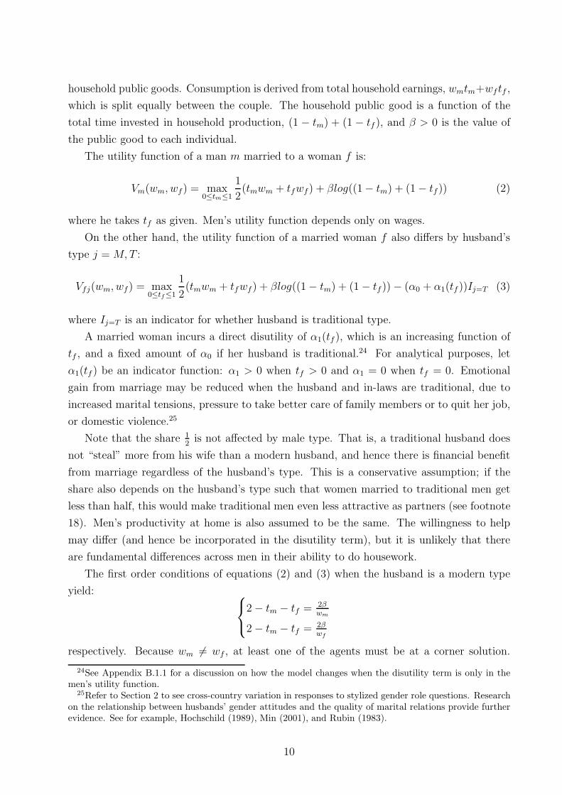
The utility function of a man m married to a woman f is:
Vm(wm, wf) = max0≤tm≤1
1
2(tmwm + tfwf) + βlog((1− tm) + (1− tf )) (2)
where he takes tf as given. Men’s utility function depends only on wages.
On the other hand, the utility function of a married woman f also differs by husband’s
type j = M,T :
Vfj(wm, wf) = max0≤tf≤1
1
2(tmwm + tfwf) + βlog((1− tm) + (1− tf ))− (α0 + α1(tf ))Ij=T (3)
where Ij=T is an indicator for whether husband is traditional type.
A married woman incurs a direct disutility of α1(tf ), which is an increasing function of
tf , and a fixed amount of α0 if her husband is traditional.24 For analytical purposes, let
α1(tf ) be an indicator function: α1 > 0 when tf > 0 and α1 = 0 when tf = 0. Emotional
gain from marriage may be reduced when the husband and in-laws are traditional, due to
increased marital tensions, pressure to take better care of family members or to quit her job,
or domestic violence.25
Note that the share 1
2is not affected by male type. That is, a traditional husband does
not “steal” more from his wife than a modern husband, and hence there is financial benefit
from marriage regardless of the husband’s type. This is a conservative assumption; if the
share also depends on the husband’s type such that women married to traditional men get
less than half, this would make traditional men even less attractive as partners (see footnote
18). Men’s productivity at home is also assumed to be the same. The willingness to help
may differ (and hence be incorporated in the disutility term), but it is unlikely that there
are fundamental differences across men in their ability to do housework.
The first order conditions of equations (2) and (3) when the husband is a modern type
yield: 2− tm − tf = 2β
wm
2− tm − tf = 2β
wf
respectively. Because wm 6= wf , at least one of the agents must be at a corner solution.
24See Appendix B.1.1 for a discussion on how the model changes when the disutility term is only in themen’s utility function.
25Refer to Section 2 to see cross-country variation in responses to stylized gender role questions. Researchon the relationship between husbands’ gender attitudes and the quality of marital relations provide furtherevidence. See for example, Hochschild (1989), Min (2001), and Rubin (1983).
10
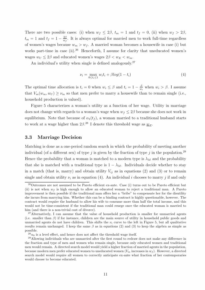
There are two possible cases: (i) when wf ≤ 2β, tm = 1 and tf = 0, (ii) when wf > 2β,
tm = 1 and tf = 1 − 2β
wf. It is always optimal for married men to work full-time regardless
of women’s wages because wm > wf . A married woman becomes a housewife in case (i) but
works part-time in case (ii).26 Henceforth, I assume for clarity that uneducated women’s
wages wU ≤ 2β and educated women’s wages 2β < wE < wm.
An individual’s utility when single is defined analogously.27
νi = max0≤ti≤1
witi + βlog(1− ti) (4)
The optimal time allocation is ti = 0 when wi ≤ β and ti = 1 − β
wiwhen wi > β. I assume
that Vm(wm, wU) ≥ νm so that men prefer to marry a housewife than to remain single (i.e.,
household production is valued).
Figure 5 characterizes a woman’s utility as a function of her wage. Utility in marriage
does not change with regards to a woman’s wage when wf ≤ 2β because she does not work in
equilibrium. Note that because of α1(tf ), a woman married to a traditional husband starts
to work at a wage higher than 2β.28 I denote this threshold wage as wE.
3.3 Marriage Decision
Matching is done as a one-period random search in which the probability of meeting another
individual (of a different sex) of type j is given by the fraction of type j in the population.29
Hence the probability that a woman is matched to a modern type is λM and the probability
that she is matched with a traditional type is 1 − λM . Individuals decide whether to stay
in a match (that is, marry) and obtain utility Vij as in equations (2) and (3) or to remain
single and obtain utility νi as in equation (4). An individual i chooses to marry j if and only
26Outcomes are not assumed to be Pareto efficient ex-ante. Case (i) turns out to be Pareto efficient but(ii) is not when wf is high enough to allow an educated woman to reject a traditional man. A Paretoimprovement is then possible if the traditional man offers her a “bribe” to compensate her for the disutilityshe incurs from marrying him. Whether this can be a binding contract is highly questionable, however. Thecontract would require the husband to allow his wife to consume more than half the total income, and thiswould not be time-consistent if the traditional man could renege once the educated woman is married tohim (and there is a non-trivial cost of divorce).
27Alternatively, I can assume that the value of household production is smaller for unmarried agents(i.e. smaller than β) if for instance, children are the main source of utility in household public goods andunmarried agents do not have children. This shifts the νi curve to the left in Figure 5, but all qualitativeresults remain unchanged. I keep the same β as in equations (2) and (3) to keep the algebra as simple aspossible.
28α0 is a level effect, and hence does not affect the threshold wage itself.29Allowing individuals who are unmarried after the first round to redraw does not make any difference in
the fraction and type of men and women who remain single, because only educated women and traditionalmen would remain. A directed search model would yield a higher fraction of married agents in the population,because modern men prefer educated women to uneducated women (Vm increases in wf ). However, a directedsearch model would require all women to correctly anticipate ex-ante what fraction of her contemporarieswould choose to become educated.
11
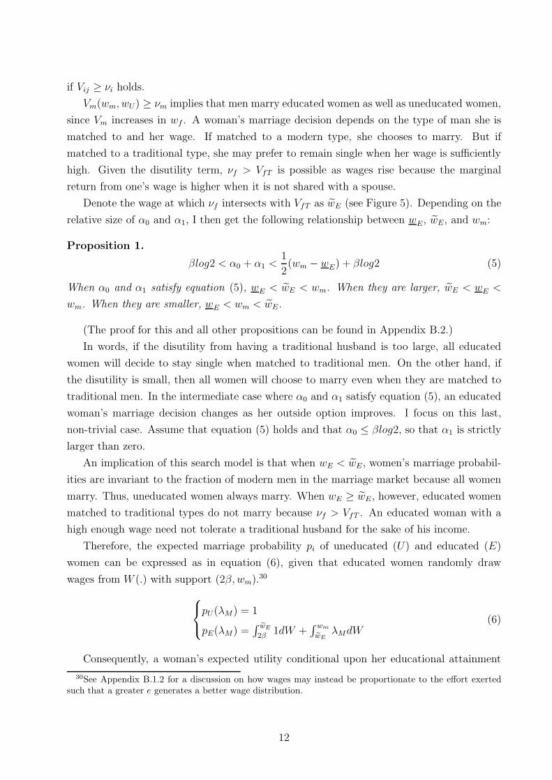
if Vij ≥ νi holds.
Vm(wm, wU) ≥ νm implies that men marry educated women as well as uneducated women,
since Vm increases in wf . A woman’s marriage decision depends on the type of man she is
matched to and her wage. If matched to a modern type, she chooses to marry. But if
matched to a traditional type, she may prefer to remain single when her wage is sufficiently
high. Given the disutility term, νf > VfT is possible as wages rise because the marginal
return from one’s wage is higher when it is not shared with a spouse.
Denote the wage at which νf intersects with VfT as wE (see Figure 5). Depending on the
relative size of α0 and α1, I then get the following relationship between wE, wE, and wm:
Proposition 1.
βlog2 < α0 + α1 <1
2(wm − wE) + βlog2 (5)
When α0 and α1 satisfy equation (5), wE < wE < wm. When they are larger, wE < wE <
wm. When they are smaller, wE < wm < wE.
(The proof for this and all other propositions can be found in Appendix B.2.)
In words, if the disutility from having a traditional husband is too large, all educated
women will decide to stay single when matched to traditional men. On the other hand, if
the disutility is small, then all women will choose to marry even when they are matched to
traditional men. In the intermediate case where α0 and α1 satisfy equation (5), an educated
woman’s marriage decision changes as her outside option improves. I focus on this last,
non-trivial case. Assume that equation (5) holds and that α0 ≤ βlog2, so that α1 is strictly
larger than zero.
An implication of this search model is that when wE < wE, women’s marriage probabil-
ities are invariant to the fraction of modern men in the marriage market because all women
marry. Thus, uneducated women always marry. When wE ≥ wE, however, educated women
matched to traditional types do not marry because νf > VfT . An educated woman with a
high enough wage need not tolerate a traditional husband for the sake of his income.
Therefore, the expected marriage probability pi of uneducated (U) and educated (E)
women can be expressed as in equation (6), given that educated women randomly draw
wages from W (.) with support (2β, wm).30
pU(λM) = 1
pE(λM) =∫ wE
2β1dW +
∫ wm
wEλMdW
(6)
Consequently, a woman’s expected utility conditional upon her educational attainment
30See Appendix B.1.2 for a discussion on how wages may instead be proportionate to the effort exertedsuch that a greater e generates a better wage distribution.
12
can be expressed as:
VU(λM) = λMVUM + (1− λM)VUT
VE(λM) =∫ wE
2β(λMVEM + (1− λM)VET )dW +
∫ wm
wE(λMVEM + (1− λM)νf)dW
(7)
where Vfj and νf are as defined in equations (3) and (4).
3.4 Education Decision
I assume that each woman faces an idiosyncratic effort cost e of becoming educated, where
e is an iid random draw from a continuous cumulative distribution function G(.). Let
e(λM) ≡ VE(λM)− VU(λM) (8)
be the expected utility differential between an educated and uneducated woman given the
fraction of modern men, λM . Because wages are exogenous, e(λM) is independent of the
fraction of women who decide to become educated.31
e(λM) has the following properties:
Proposition 2. e(λM) is an increasing function of λM , and e(λM) ≥ 0 always holds.
Since all women with effort cost e ≤ e(λM) decide to invest in education, the equilibrium
λE(λM)—fraction of educated women—at any point in time is:
λE(λM) = G(e(λM)) (9)
It follows directly from Proposition 2 that λE(λM) is also a continuous, increasing function
of λM on [0, 1). λE = 1 (and therefore λM = 1) is ruled out, because e can be unboundedly
large. In words, more women find it worthwhile to invest in education when there is a larger
fraction of modern men because marriage prospects are better. But it is never the case
that all women become educated because there are always a few whose cost of investing in
education is very high.
3.5 Shock to Women’s Wages and the Gold Miss Phenomenon
There are equal numbers of men and women in the society. Let the number of educated
women at period t be denoted as FEt:
FEt ≡ λEt(λMt)Ft (10)
31I abstract from general equilibrium effects on wages.
13
where Ft is the total number of women at t. The conditional probability of being unmarried
when educated (being a Gold Miss), is simply 1− pE(λMt) , where pE(λMt) is the marriage
probability of educated women as defined in equation (6).
Wt(.) is the continuous cumulative distribution function of educated women’s wages in
generation t over support (2β, wm). The following comparative statics can be made with
regards to contemporaneous wages:
Proposition 3. Given Wt−1(.) and λMt−1, if the distribution Wt1(.) first-order stochastically
dominates Wt2(.), FEt1 ≥ FEt2.
Proposition 4. Given Wt−1(.) and λMt−1, educated women’s marriage probability is an
increasing function of Wt(wE). Hence if the distribution Wt1(.) first-order stochastically
dominates Wt2(.), pEt1 ≤ pEt2.
That is, both the number of educated women and the probability that they remain un-
married are increasing in educated women’s current wages. Proposition 3 is straightforward;
more women are incentivized to invest in education when the returns to education are greater.
Proposition 4 results because women with wages higher than wE can afford to stay single
when matched to traditional men.32
More important, however, is whether the probability of becoming a Gold Miss increases
or decreases as wages rise over time, i.e. pEt − pEt−1.33
Proposition 5. Suppose Wt(.) first-order stochastically dominates Wt−1(.) at all t. The
decrease in pE from t− 1 to t is larger when (i) the drop in W (wE) from t− 1 to t is larger
and (ii) the shift in W (.) from t− 2 to t− 1 is smaller.
That is, the Gold Miss phenomenon is more likely to arise in economies where there was a
large, one-time shock to women’s wages than in those that had a more gradual wage growth.
To understand why this is so, notice that wage increase affects pE in two opposite di-
rections. First, there is the contemporaneous effect: higher wages allow educated women
to remain single when matched to traditional type and thus lowers marriage probability
(Proposition 4). On the other hand, more women have an incentive to become educated
when wages are high (Proposition 3) and this generates a larger fraction of modern males in
the next generation. This intergenerational effect raises educated women’s marriage prob-
ability by increasing the pool of marriageable men. The second effect, unlike the first, is
lagged.
32Comparative statistics of Proposition 4 cannot be summarized with just the mean of W (.). With first-order stochastic dominance, the mean increases with time. However, in the perverse case of the distributionchanging without affecting W (wE), an educated woman’s marriage probability would remain constant re-gardless of the change in means (since all women with wages below wE get married). In other words, growthin women’s wages “on average” is not a sufficient condition for a decrease in pE .
33Since uneducated women always marry, pUt − pUt−1 = 0.
14
Condition (i) in Proposition 5 enlarges the first effect whereas condition (ii) curtails the
second, resulting in the Gold Miss phenomenon. But if either of the conditions fail to hold,
the two opposing effects come into play and pEt may fall only slightly relative to pEt−1, or
may even increase.
In sum, the Gold Miss phenomenon should be best observed when there is a shock to
women’s wages in a country with a large fraction of traditional men. The key observation
is that the results do not depend on societies being endowed with different types of men.
Even if all countries had equally traditional men at t = 1 and the same wage level at t = T ,
mismatch in the marriage market would be a function of how rapidly the economy grew
between t = 1 and t = T . Therefore, similarly developed countries at t = T can have very
different gender norms, which in turn dictates the variation in the degree of mismatch we
observe in the marriage market.
Finally, it is worth noting that this path dependency feature may result in prolonged
repercussions, well beyond the arising of the Gold Miss phenomenon. Countries may become
“stuck” in the Gold Miss equilibrium because as long as the Gold Misses do not have children,
they cannot contribute to producing a new cohort of modern males. But if the fraction of
modern men depends on the fraction of all educated women in the previous cohort (regardless
of marital status), then the fraction of modern men would increase greatly after the Gold
Miss generation.
4 Evidence on the Effect of Cultural Transmission on
the Gold Miss Phenomenon
I focus my empirical exploration of the model on four testable implications. First, men who
grew up around highly educated women are less traditional than those who grew up around
less educated women. Second, husband’s type affects household time allocation; a woman is
more likely to work in the labor market when her husband is a modern type. Third, women
marry less traditional men (rather than traditional) when they are available. Fourth (and
as a consequence of the prior points), the Gold Miss phenomenon is less severe when there
is a larger fraction of modern men in the marriage market.
The ideal way to test these predictions would be to exogenously vary wage growth paths
or the composition of male types within an initially traditional country and then see how
the marriage market unfolds generations later. Because this is not feasible, I use three
different datasets—the Japanese General Social Survey, the U.S. Census and the American
Community Survey, and the American Time Use Survey—to test the four elements above.
15
4.1 Gender Attitudes and Marriage Patterns in Japan
I first analyze the Japanese General Social Survey (JGSS) to evaluate how a mother’s edu-
cation and employment affect her son’s gender attitudes and marriage patterns in one of the
Gold Miss countries—Japan.
4.1.1 Data
The JGSS is designed to solicit political, sociological, and economic information from men
and women living in Japan and has been conducted seven times during the 2000s.34 I pool
these years for the analyses. The sample size is about 3,500 per year. Observations are always
weighted to make the sample representative of the Japanese population.35 Respondents
younger than 25 or still attending school are excluded in order to obtain more accurate data
on final education.
Appendix Table A1 contains descriptive statistics of the key variables. Only 3 percent of
the respondents have college graduate mothers, because as mentioned in Section 2, not until
the education reform after World War II could women attend college and even then many
attended junior (two-year) colleges.
4.1.2 Results
My model rests on the notion that gender norms are subject to change and that men’s views
of gender roles are influenced by their mothers. I investigate this using individual’s responses
to five questions in the JGSS specifically designed to capture gender attitudes.
Respondents are asked whether they agree or disagree with the following statements: “If
a husband has sufficient income, it is better for his wife not to have a job,” “Men should
cook and look after themselves,” “A husband’s job is to earn money; a wife’s job is to look
after the home and family,” “A preschool child is likely to suffer if his/her mother works,”
and “It is more important for a wife to help her husband’s career than to have one herself.”
An individual can be defined as less traditional if he/she agrees with the second statement,
and disagrees with the other statements.
Figure 6 depicts the trend of the responses to these five statements across birth cohorts.
The “less traditional index” ranges from 0 to 5: it equals 5 if the individual responded
less traditionally to all five questions (whether that corresponds to agreeing or disagreeing
depends on the specific statement). Women are less traditional than men and the gap is
larger in recent cohorts. Also, there has been a significant evolution of beliefs for both men
and women over time. Those who were born after 1960 responded less traditionally to at
least one or two more statements compared with those born in the 1920s.
342000, 2001, 2002, 2003, 2005, 2006, and 2008.35See Appendix A.3 for how the weights are constructed.
16
To investigate whether the mother-to-son transmission exists, I estimate the following
linear probability model:
Yist = β0 + β1Xist + β2MomLFPist + β3MomCollist + γt + δs + εist (11)
where the dependent variable Yist is an indicator variable that equals 1 if the response to
the specific question (listed above) is less traditional for a man i who lives in region s and
belongs to cohort t. MomLFPist equals 1 if his mother had a paying job when he was about
15 years old, and MomCollist equals 1 if his mother is a college graduate.36 Xist represents
a set of demographic controls such as respondent’s age, education, and income. In addition
to regional and urban dummies δs, I include cohort fixed effects γt to take into account the
time trend observed in Figure 6.37
Table 1 contains the estimation results. The coefficients on having had a working and
college graduate mother are always positive, and are statistically significant in cols. 1, 3, and
4. The probability that a man disagrees with the statements “If a husband has sufficient
income, it is better for his wife not to have a job,” “A husband’s job is to earn money; a
wife’s job is to look after the home and family” and “A preschool child is likely to suffer if
his/her mother works” increases by about 5 percentage points if his mother worked relative
to if his mother did not work when he was young and by more than 10 percentage points if
his mother is a college graduate. These are comparable in magnitude to the marginal effect
of the respondent himself being college graduate. Father’s educational attainment, on the
other hand, has no statistically significant effect. The results are robust to restricting the
sample to currently married men.38
If men who had working and/or college graduate mothers are indeed less traditional, are
they more likely to be married than men who had housewife mothers? And are their wives
more likely to work after marriage?
To address the first question, I look at the correlation between a mother’s background and
her son’s marriage probability. Table 2 shows that there is a small but positive relationship
between a mother’s LFP and her son’s marriage probability (col. 1). To reduce the bias from
potential correlations between a mother’s work status and her son’s ability, and since the
36The JGSS asks “When you were about 15 years old, did your mother have any paying job? If so, whatdid she do?” MomLFPist is zero for those who answered “She was not working.” Respondents who “Don’tknow” or did not have a mother at that time are excluded. MomCollist equals 1 for four-year colleges (notjunior college or college of technology).
37There are 47 prefectures in Japan, which are governmental bodies larger than cities, towns, and villages.The prefectures are grouped into six regions (“blocks”) in the JGSS. Urban is a set of three dummies forthe size of municipality—largest cities, other cities, and town/village. Largest cities are the “Cabinet-Orderdesignated cities” that have more than 500,000 people.
38When I replicate this analysis for female respondents, I find that both mother’s LFP and mother beinga college graduate do not have statistically significant effects on women’s gender attitudes. Consistent withthe model’s assumption, the intergenerational transmission of gender attitudes matters more for men thanwomen.
17
model focuses on the case where men’s wages are higher than women’s, I run the regression
for just the college graduate men in col. 2. I find that mother’s LFP has a larger positive effect
than when all men are considered. As for mother’s educational attainment, the coefficient is
positive but statistically insignificant. Thus, a man’s likelihood of marriage is higher if his
mother worked or is a college graduate.
To address the second question, I estimate equation (11) with wife’s current labor force
participation (measured by whether she had any paying job in the last week) as the dependent
variable. Table 3 contains the results. Having a college graduate mother does not have a
statistically significant effect on wife’s probability of working. But a man having had a
working mother when he was young raises the probability that his wife works by about
6 percentage points. When the sample is restricted to college graduate men, the effect is
7.2 percentage points. This is more than a 10 percent increase since the mean of married
women’s LFP is about 50 percent.
Note that region, urban, and rural at age 15 dummies are included to control for regional
variation; places with female-dominated industries may bias the mere chance that both
mother and wife are employed. Wife’s LFP is negatively correlated with husband’s education,
income, and the total number of children in the household. It is positively correlated with
herself being college graduate. Using wife’s usual hours worked per week instead of her LFP
as the dependent variable yields similar results.39
Altogether, these results suggest that a mother’s work experience and educational attain-
ment affect her son’s gender attitudes and marriage. Consistent with the model’s assumption
on intergenerational transmission, men who had working and college graduate mothers are
more likely to have egalitarian gender attitudes. The probability that a man ever marries
and that he has a working wife also increases with his mother’s LFP and education.
4.2 Time Use of Married Immigrants in the U.S.
We have just seen that Asian men are tradition-bound but are less so when their mothers
are more educated and work more outside the home. The supply of modern men in Asia
is therefore limited. What happens when educated Asian women live in areas with more
modern men? In this section, I explore time use of married immigrants in the U.S. to see
whether a husband’s type—as proxied by his country of origin and U.S. nativity—affect his
and his wife’s time spent on household chores.
39The coefficient on mother’s LFP is 3.4 hours per week for all men and 4.1 hours per week when thesample is restricted to college graduate men. They are both statistically significant at the 1 percent level.
18

4.2.1 Data
I use the 2003–2011 waves of the American Time Use Survey (ATUS) to explore the time
spent by respondents (and their household members) on both market and non-market ac-
tivities. Because the survey is also linked to the Current Population Survey, which contains
information on father’s and mother’s birthplace for all respondents, I am able to identify
an individual’s country of origin. Because the sample size of those from Gold Miss coun-
tries (Hong Kong, Japan, Korea, Taiwan, and Singapore) is small, I expand my analyses to
those from “traditional” and “less traditional” countries in general. (Results for Gold Miss
countries only are reported in the Appendix.)
I use female labor force participation (FLFP) rates in father’s birthplace to divide coun-
tries into traditional and less traditional groups.40 The United Nations (UN) provides data
(from the International Labor Organization) on women’s share of labor force in 187 countries
starting from 1985. To focus on adult women’s LFP and to obtain statistics for as many
countries as possible, I use the FLFP rate of the 25–34 age group. I also use the oldest data
available, 1985, to better reflect the gender norms that immigrants were exposed to before
migrating to the U.S.
I define high (low) FLFP countries as countries where women’s LFP rates in 1985 were
higher (lower) than that of the U.S.—70.9 percent. U.S. is used as the standard since the
shift in gender norms that immigrants experience derives from the contrast between their
country of origin and the U.S. A total of 121 countries in the UN data are matched to
father’s birthplace in the ATUS sample, of which 42 countries are high FLFP and 79 are low
FLFP. (See Appendix Figure A2 for a map of the countries by category.)
For all analyses in this section, only married couples with spouse present are considered
since couples who are currently separated or divorced do not face the same constraints in
determining time allocation as couples living together. Couples with either respondent or
spouse under age 25 are excluded. In comparing across generations, I distinguish between for-
eign born, second generation, and third and higher generations. All foreign born immigrants
are categorized as foreign born regardless of their age at migration.41 Second generation is
U.S. born respondents whose fathers are foreign born. Third and higher generations are U.S.
born respondents whose fathers are also U.S. born.
Appendix Table A2 contains the summary statistics of my sample. Immigrants with
40I can alternatively use mother’s birthplace and the results are similar (95 percent of respondents haveparents born in the same country). FLFP is commonly used in the political economy literature as an indicatorof a country’s family culture and women’s economic status. See for example, Alesina and Giuliano (2010)and Fernandez and Fogli (2009). For my purposes, married women’s LFP rates would be ideal, but they arenot available in cross-country datasets.
41There are no respondents who are foreign born yet with a U.S. born father in the sample, reducing thepossibility of bias from adoptees. I also do not exclude those who have migrated to the U.S. as adults becauseunlike education and marriage decisions in Section 4.3 below, time use at home within married couples is aneveryday practice, and thus is not contingent on the decisions made back home.
19
low FLFP origin compose more than 80 percent of foreign born and 70 percent of second
generation men and women. By definition, the fraction is zero for third and higher genera-
tions. Among those with low FLFP origins, about 40 percent of them are from Mexico in
the foreign born group; hence, I include a dummy for Mexican origin in all my analyses.
4.2.2 Results
There are several ways to group non-market activities. I have chosen to use “core non-market
work” in Guryan, Hurst and Kearney (2008), which includes activities such as food prepa-
ration, indoor cleaning, and washing/drying clothes. Time spent on shopping, and other
home production such as home maintenance, outdoor cleaning, vehicle repair, gardening,
and pet care are excluded, as well as time spent on child care, medical care, education, and
restaurant meals. Throughout, I refer to “core non-market work” as housework.42
Figure 7 summarizes the time spent on housework by sex, generation, and country of
origin. Married men spend on average five hours or less on housework and married women’s
hours are about three times longer. For women from high FLFP countries, hours stay roughly
constant across generations. For women from low FLFP countries, there is a clear reduction
across generations: the mean of housework time falls by about six hours—from 21.8 hours per
week among the foreign born to 15.6 hours per week among the second generation. Variation
among married men is much smaller: there is less than an hour increase from foreign born
to U.S. born among those from low FLFP countries.
According to the model, men from countries where most women work (high FLFP origin
or U.S. born) are more likely to be the modern type than those who grew up in countries
where most women are housewives (foreign born from low FLFP countries). Since Figure 7
does not control for systematic differences that may exist between different groups, I estimate
the following equation to investigate the effect of cultural background on men’s housework
hours:
Yist = β0 + β1Xist + β2U.S.bornist + β3thirdist + γt + δs + εist (12)
where the Xist are demographic controls such as age, education, usual work hours, the
number of children in household, the age of the youngest child in household, and race, and
year (γt) and state (δs) fixed effects are included.43 The variable U.S.bornist equals 1 if the
respondent is U.S. born and 0 if foreign born. thirdist equals 1 if respondent is third or
higher generation and equals 0 otherwise; hence, together with U.S.bornist, I am able to
distinguish between foreign born, second, and third or higher generations. Standard errors
42All findings are robust to using a broader definition that includes other home production activities, suchas “total non-market work” in Guryan, Hurst and Kearney (2008).
43Usual work hours are only available for individuals who are employed. I recode the variable to zero forthose currently unemployed. Individuals who responded “hours vary” are excluded from the analyses. Racehas 21 categories and includes multiple-race in addition to all major single race classifications.
20
are clustered by father’s birthplace.
Table 4 shows the OLS regression results, separately for men from low FLFP countries
and high FLFP countries. For men from low FLFP countries (cols. 1 to 3), the key variable of
interest is U.S. born. (This refers strictly to second generation since, by definition, there is no
third or higher generation with low FLFP origin.) The coefficient is positive and statistically
significant. Taking into account working hours and family characteristics, a U.S. born man
with a low FLFP origin spends about 0.8 more hours on housework than a foreign born one,
a non-trivial difference considering that the mean housework time for men is 4.5 hours per
week.
Unsurprisingly, being U.S. born matters less for men from high FLFP countries (cols.
4 to 6). The marginal effect of being U.S. born and the additional effect of being third or
higher generation are both statistically insignificant when all the controls are included.44
To rule out the potential concern that the results are driven by ethnic composition ef-
fects, I repeat the analysis above for men from Gold Miss countries only. Of course, the
Gold Miss countries—Hong Kong, Japan, Korea, Singapore, and Taiwan—are all in the low
FLFP category. Table 5 presents the estimates from the OLS regression. Despite the small
sample size, the coefficient on U.S. born is large and highly significant. Relative to foreign
born, Asian American men spend about four hours more on housework when the couple’s
demographics and working hours are considered (cols. 1 and 2) and 2.5 hours more when the
number and age of children are considered as well (col. 3).
Thus, modern husbands—U.S. born and/or from high FLFP countries—spend more time
on housework than traditional husbands, taking into account couple’s demographics, working
hours, and children. However, the difference is much smaller than the variation in women’s
housework hours observed in Figure 7. In fact, given that men earn higher wages than women
in most families, the important distinction between modern and traditional type males may
not be in their own housework hours but in how much they desire the housework to be done
by their wives. The model predicts that a woman married to a traditional husband does
more housework than a woman married to a modern one, ceteris paribus.
I investigate the effect of husband’s cultural background on wife’s housework hours, and
I focus on women from low FLFP countries.45 The regression is similar to equation (12)
44These results are also robust to a more general definition of traditionality. In Appendix Table A3, Iuse the actual FLFP rate in the respondent’s father’s birthplace instead of the dichotomous distinction ofhigh and low FLFP origins. Consistent with the findings above, the marginal effect of being U.S. born andthe marginal effect of the FLFP rate are both positive while the interaction between FLFP rate in father’sbirthplace and U.S. born is negative. That is, the difference in housework time between U.S. born andforeign born is smaller among men from countries with higher FLFP rates.
45Women from high FLFP countries are rarely married to traditional men—both by origin and U.S.nativity standards. Among married women with high FLFP origins, only 4.7 percent have husbands withlow FLFP origins and only 4.6 percent have husbands who are foreign born. There is variation in husband’sbackground among married women with low FLFP origins, however. 27 percent of them have husbands withhigh FLFP origins and 37 percent of them have husbands who are U.S. born.
21
but with husband’s country of origin and generation since migrating to the U.S. as the key
covariates, and standard errors clustered by husband’s father’s birthplace.
Table 6 contains the estimation results. Col. 1 shows that having a husband from a low
FLFP country increases a woman’s housework time by about three hours per week compared
with having a husband from a high FLFP country. When only U.S. nativity is considered,
col. 2 indicates that husbands who are third generation show the opposite effect: they lower
wives’ housework time by three hours. When both husband’s country of origin and U.S.
nativity are included as covariates in col. 3, husband’s origin remains large and significant
(the magnitude is larger than the effect from the woman herself being U.S. born) whereas
the coefficient on husband’s U.S. nativity loses significance.
In Table 7, I repeat the exercise above with just the women from Gold Miss countries.
The sign of the coefficients on husband’s origin and U.S. nativity are the same as in Table
6 and the size of the coefficients are even larger: country of origin and husband being third
generation have marginal effects of about six hours per week when considered separately
(cols. 1 and 2). When both are included as covariates in col. 3, the average housework time
of Asian women married to third generation men is about 8.9 hours less than those married
to foreign born or second generation men. The magnitude translates into more than a 50
percent drop in married women’s housework time.
These results are consistent with the prediction that variation in housework hours of
married women can be partly attributed to husbands’ cultural backgrounds. The type of
the men matters not so much because men do the housework but because they do not mind
their wives’ doing less and outsourcing more.
Furthermore, the findings above imply that cross-country differences in family-friendly
environment or substitutability between household production and market goods cannot be
the main determinant of the Gold Miss phenomenon. As mentioned in Section 2, not only
are the relative prices of outsourcing housework in the U.S. and East Asia similar, but as
shown here, there is a wide cultural variation in household time allocations even among those
living in the same country.
4.3 Marriage Patterns of Koreans and Japanese in the U.S.
My research and others suggest that immigrants are culturally similar to those in their home
countries and U.S. born men are less traditional than Asian born men.46 Thus, immigration
from the Gold Miss countries to the U.S. can demonstrate how the marriage market equi-
librium would change when more modern males become available in Asia. I use the U.S.
census data to examine whether the Gold Miss phenomenon similarly exists among Koreans
and Japanese in the U.S., and if not, whom the women are marrying in the U.S.
46See footnote 8 for references on U.S. immigrants’ cultural and economic assimilation.
22
4.3.1 Data
I use the 1980, 1990, 2000 Census and the 2001 to 2010 American Community Survey (ACS)
IPUMS files.47 A respondent is defined as Korean or Japanese if categorized as “Korean” or
“Japanese” in the single race variable.48 (Hong Kong, Taiwan, or Singapore is not recognized
as single race categories. They are grouped as “Other Asian” or “Chinese.”) Individuals
younger than 25 or still attending school are excluded.
I distinguish between first and higher generations of immigrants. Because immigrants
may have chosen to come to the U.S. after completing their final education in their home
countries or getting married, bringing their spouses with them, I only use respondents who
immigrated to the U.S. when they were younger than 18 years old. I also exclude respondents
who migrated before three years old to limit the bias from including Korean and Japanese
adoptees.49 Foreign born in this section refers to immigrants who came to the U.S. between
ages 3 and 17. Second and higher generations are grouped as U.S. born.50
Appendix Table A4 reports the descriptive statistics of my sample. Foreign born are
comprised of fewer Japanese because the wave of immigration from Korea has been more
recent. Hence, I control for respondent’s ethnicity in all my analyses.
4.3.2 Results
Before moving to the main empirical tests, I examine the educational attainment of Koreans
and Japanese in the U.S. Figure 8 plots the fraction college graduate by sex, nativity, and
cohort. During the past 50 years, the percentage of four-year college graduates among Korean
and Japanese women increased from less than 20 percent to more than 60 percent. Although
there were more male college graduates in the early cohorts, the increase was more gradual
47The Census and the ACS are the only datasets that have sufficiently large sample size to study theKoreans and Japanese in the U.S.
48The Census and ACS collect parent’s birthplace only for respondents who live with their parents atthe time of the survey (less than 5 percent of the adult population). Single race is assigned accordingto respondent’s self-reported race in the survey and is comparable across all years and is available for allrespondents (including those with multiple-race). Individuals with multiple-race are assigned to the singlerace category deemed most likely. However, multiple-race is extremely rare among Koreans and Japanese:99 percent of Koreans and 98 percent of Japanese self-reported themselves as “Korean” or “Japanese” inthe detailed race question (and not “Korean and White” or “Japanese and White,” for instance).
49See Appendix A.5 for how age at migration is calculated. Adoptees may be identified as Korean orJapanese in the Census despite having been brought up by American parents and not having any culturalconnections to Korea or Japan. According to the Intercountry Adoption statistics from the U.S. Departmentof State, 99 percent of adoptees from Korea and Japan in 1999–2011 arrived in the U.S. when they wereyounger than three years old. The Holt International Children’s Services data in Sacerdote (2007) also showssimilar figures for Korean adoptees placed during 1964–1985: 91.4 percent of children arrived under the ageof three.
50It is impossible to distinguish between these generations without information on parent’s birthplace.Since the immigration wave from East Asia began in the 1960s (after the Immigration and Nationality ActAmendments of 1965), third or higher generations are expected to comprise a small fraction of my sample.Naturalized citizens are not categorized as U.S. born.
23
for men, resulting in a switch in the educational gender gap. The overall development across
time is similar for the foreign born and the U.S. born, with levels reaching about 60 percent
from the 1970s birth cohort for both men and women. Hence, the fraction college graduate
is larger among Koreans and Japanese in the U.S. than among white Americans (less than
40 percent).
The Gold Miss phenomenon among Koreans and Japanese who immigrated to the U.S.
may well be more severe because the sex ratio among college graduates in the U.S. is less
in favor of women than in Korea and Japan, where there are more male than female col-
lege graduates (see Figure 2). However, Figure 9 shows that college graduate Koreans and
Japanese are as likely to be married as the non-college graduates. For both sexes, the frac-
tion married among college graduates relative to non-college graduates has been increasing
across cohorts, and the difference switched from negative to positive for women. This con-
trasts starkly with the downward trend found in Asia and is instead similar to the trend
observed among Americans overall (see Figure 4). The Gold Miss phenomenon does not hold
in the U.S.
Because women’s educational attainment, labor force participation, and wages increased
decades earlier in the U.S. than in Asia, men who grew up in the U.S. have less traditional
gender attitudes than those who grew up in Korea and Japan. College graduate women
would then have greater options in the U.S. marriage market than in Korea or Japan.
This notion appears to have much validity. Among the college graduate and foreign born
Koreans and Japanese (Table 8 Panels A and B, row 1), women are much more likely than
men to have a spouse who is neither Korean nor Japanese. The gender gap is large: one third
of these women married U.S. born who are not Korean or Japanese while only 16 percent of
men did, and about half of the women married foreign born Korean or Japanese while more
than 70 percent of men did.
The gender gap in spouse’s ethnicity is smaller among the U.S. born Koreans and
Japanese (Panels A and B, row 2). The incidence of having a foreign born Korean or
Japanese spouse falls to 6 percent for women and 12.5 percent for men. The vast majority
of both sexes marry U.S. born—89 percent of women and 81 percent of men—although men
tend to marry Korean or Japanese Americans while women tend to marry Americans who
do not identify themselves as Korean or Japanese (mostly white). The differential mar-
riage pattern by respondent’s sex and U.S. nativity are robust to including respondent’s age,
education, ethnicity, and state and cohort fixed effects (see Appendix Table A5).
Thus, my findings suggest that Korean and Japanese men and women have different
preferences for their spouse’s ethnicity and U.S. nativity. Korean and Japanese men (par-
ticularly foreign born) usually marry Korean or Japanese immigrants whereas Korean and
Japanese women (even those who are foreign born) marry Americans.
To test whether women’s inclination to marry out of their ethnic group can be explained
24
by the Korean and Japanese men being more traditional than American men, I exploit
regional variation in the composition of the Korean and Japanese male population. That is,
for each state-cohort cell (six decennial birth cohorts and 51 states, including the District
of Columbia), I calculate the fraction foreign born among Korean and Japanese men—
number of foreign born Korean and Japanese men divided by the total number of Korean
and Japanese men. A larger share means that there are more foreign born than U.S. born
among the Korean and Japanese men in respondent’s state and cohort.51
The estimating equation is the following linear probability model:
Yist = β0 + β1Xist + β2fracfbst + β3totalst + γt + δs + εist (13)
where the dependent variable is an indicator variable that equals 1 if husband is not Korean
or Japanese and 0 otherwise. The key covariates fracfbst and totalst are, respectively, the
fraction foreign born among Koreans and Japanese men and the total number of Koreans and
Japanese men in the respondent’s state s and cohort t.52 The usual demographic controls
are included. Cohort fixed effects absorb common time trends that may exist with regards
to immigration from Asia or discrimination against interracial marriage. State fixed effects
control for differences across states such as the type of industries and racial composition.
Standard errors are clustered at the state-cohort level.
Table 9 presents the result of estimating equation (13) separately by education and U.S.
nativity of Korean and Japanese women. The positive coefficient on fraction foreign born
among Korean and Japanese men shows that the probability a Korean or Japanese woman
marries out of her ethnic group increases when there are fewer U.S. born among the Korean
and Japanese men in her state-cohort. Moreover, consistent with the model’s assumption
that the disutility from having a traditional husband is greater for educated women than for
uneducated women, the coefficient is larger in magnitude for college women (cols. 1 and 2)
than for non-college women (cols. 3 and 4).
The results are not driven by differences in the chance of meeting a Korean or Japanese
of the opposite sex or the competition between Koreans and Japanese of the same sex in
the marriage market; I control for both the total number of Korean and Japanese men and
women in the respondent’s state and cohort and also the fraction foreign born within the
female population. Therefore, the findings imply a causal relationship between a Korean or
Japanese woman’s decision to marry outside her ethnic group and the composition of men
in her own ethnic group.
Repeating the analysis for Korean and Japanese men shows that the fraction foreign born
51Pooling all state-cohort cells, the fraction foreign born among Korean and Japanese men ranges from 0to 1 and has mean of 0.51 and standard deviation of 0.29. Hawaii and Idaho have low fraction foreign bornwhereas New Jersey and New York have high fraction foreign born among Korean and Japanese men.
52State here refers to the state of current residence. Note that state of birth cannot be used because ofthe foreign born group.
25
among the Korean and Japanese women in respondent’s state and cohort does not have a
statistically significant effect. That is, Korean and Japanese men’s preference for Asian wives
do not respond sensitively to the composition of the female population (see Appendix Table
A6).
One potential concern with the interpretation that Korean and Japanese women marry
American men because they are modern is that white men might marry Korean and Japanese
women expecting them to be obedient housewives. Another is that Korean and Japanese
women might marry Americans to “marry-up” in socioeconomic status.
To address the first concern, I examine Korean and Japanese women’s LFP after mar-
riage. Table 10 contains OLS estimates from regressing Korean and Japanese women’s LFP
on own and spouse’s characteristics (including the husband’s income) and the number of
children in household. For foreign born Korean and Japanese women, having a husband
who is not Korean or Japanese increases the probability of working by 9.3 percentage points.
The coefficient on husband being U.S. born is statistically insignificant.53 As for U.S. born
Korean and Japanese women, both husband’s nativity and ethnicity do not have statistically
significant effects on women’s LFP though positive in sign. Using alternative definitions of
work status, such as usual hours worked per week, yields similar results.54 Thus, it does not
seem likely that Korean and Japanese women who are married to American men are very
traditional.
To address the second concern, I look at the relationship between husband’s ethnicity
(and U.S. nativity) and his education level relative to his wife’s.55 Table 11 presents the
estimates from regressing an indicator variable that equals 1 if the respondent’s husband
has higher educational attainment than herself (i.e., she is marrying-up). I run separate
regressions for foreign born and U.S. born Korean and Japanese women. The hypothesis
that an American husband has higher relative education can be rejected for both groups.
Chen and Takeuchi (2011) similarly find using the National Latino and Asian American
Survey that Asian women in the U.S. who marry non-Asians are not marrying-up in terms
of education or occupation status.
In summary, female Korean and Japanese college graduates in the U.S. are as likely to be
married as are non-college graduates. In terms of spouse’s type, Korean and Japanese women
in the U.S. are much more likely to marry Americans than their male peers, particularly
when the fraction of first generation immigrants is large within the Korean and Japanese
male population. Korean and Japanese women’s LFP after marriage and their education
53This is because as seen in Table 8, almost all foreign born women either marry a foreign born Koreanor Japanese or a U.S. born who is not Korean or Japanese, and hence the two covariates are collinear.
54When usual hours worked per week is the dependent variable, the coefficient on husband not beingKorean or Japanese is 2.5 and statistically significant at the 10% level.
55Education is used as a proxy for socioeconomic status because it is highly predictive of potential earningsand is also available for all sample (including the non-working) unlike income or occupation data.
26
levels relative to their husbands’ suggest that the observed marriage patterns are not driven
by the selection of American men who want housewives or the marrying-up of Asian women.
5 Conclusion
The “East Asian tigers” transformed into developed economies in less than 50 years. Today,
women’s educational attainment and labor market performance in this region have become
comparable to, or even surpassed those of other developed countries. In contrast to the
U.S., however, marriage rates of college graduate women in Asia have become lower relative
to that of non-college graduate women. The low marriage rates of college educated Asian
women has been termed the “Gold Miss” phenomenon.
I argue that the Gold Miss phenomenon arises in traditional societies that underwent
rapid growth in women’s wages. Rapid improvement in women’s economic status creates
a gap between the women’s role that men grew up observing and the role that the new
generation of educated women choose to take. I test my hypothesis using data from Japan
and the U.S. In Japan, I find that a mother’s working status and educational attainment are
positively correlated with her son’s gender attitudes and his likelihood of having a working
wife. In the U.S. time use data, I find that husbands from countries with low female labor
force participation rates, like the Gold Miss countries, increase wives’ housework burden. Fi-
nally, women from Korea and Japan—two major Gold Miss countries—have greater options
in the U.S. marriage market because they can marry American men instead of Korean and
Japanese men. Indeed, in the U.S., Korean and Japanese college women are as likely to be
married as non-college women.
Overall, this paper provides an explanation for why the Gold Miss phenomenon arose
in developed Asian countries and also identifies the driving forces behind the evolution of
educated women’s economic and household role.
27
A Data Appendix
A.1 Korean Data
The Korean Population Census is collected by the National Statistical Office every five yearsand are 2 percent samples of the population, excluding the institutionalized. Micro-data isavailable for years 1995, 2000, and 2005. The 2005 data does not distinguish between four-year colleges and less than four-year colleges, however, and hence I only use the 1995 and2000 samples (N = 1, 756, 493). For the most recent cohorts, I use the Korean EconomicallyActive Population Survey instead. It is collected monthly and covers individuals age 15 andolder (both in and out of labor force) in Korea. I pool all months of 2012 (N = 327, 865).
A.2 Hong Kong Data
The 2006 Hong Kong Population By-Census is collected by the Hong Kong Census andStatistics Department and is a 5 percent sample of the population (N = 460, 197). Edu-cational attainment is defined using the variable EDUCNH (highest level completed). Thefour groups corresponding to high school, junior college, college, and graduate school are:senior secondary, post-secondry (non-degree), post-secondary (degree), and graduate school.More specifically, senior secondary includes secondary forms 4 to 7; post-secondary (non-degree) includes various diploma courses and vocational training schools; post-secondary(degree) includes degree institutions; graduate level includes master degree, PhD, and otherpostgraduate courses.
A.3 JGSS
The JGSS has a variable WEIGHT to weight data for population estimates based on theJapanese Population Census. In the 2000–2005 datasets, this is produced by calculatingthe number of people which one respondent represents by taking into account sex (twocategories), 10–year age group (six categories), region (six categories), and city or not (twocategories). From 2006, the variable is produced by sex (two categories) and 10–year agegroups (seven categories). In order to attach weights across survey years, I harmonize thisvariable so that weight is constructed from sex (two categories) and 10–year age group (sixcategories) for all years in my sample.
Income (SZINCOMX, SSSZINCM) reports the total annual income during the previousyear (before taxes and other deductions) from main job. This is converted into 1999 yenusing the Consumer Price Index adjustment factors. All top-coded values in each year aremultiplied by 1.45.
In the 2008 survey, age is reported in intervals. I construct respondents’ exact age bysubtracting birth year (which is available across all years) from the year of the survey.Respondents under age 25 are excluded from the sample. However, birth year for spouse isnot provided. Hence, I take the midpoint of each 10–year age group for the spouse. Theintervals range from age group 20–29 to 90–99. Hence, spouses who are actually under age25 may be included in the analyses.
To control for the number of children when analyzing married women’s labor force par-ticipation, we need to know the number of children (under a certain age) who are currentlyliving with the respondent. Total number of children (CCNUMTTL) variable in the JGSS,however, counts both those who left home or are deceased. Hence, I construct a variable
28
that counts the number of children under 19 living with the respondent by compiling the ageof each child (CC01AGE, CC02AGE, etc.) as reported by the respondent. Because child’sage is categorical data in 10–year age groups, I use 19 as the cut-off (instead of 18, as inother datasets).
A.4 ATUS
I weigh all observations using the person weight (WT06) to make the sample representative.Family income (FAMINCOME) includes the income of all members of the household who are15 years of age or older. Income includes money from jobs, net income from business, pen-sions, dividends, interest, Social Security payments, and any other monetary income receivedby family members. This is the only earnings information available on the self-employed aswell. It is based on categorical data; I calculate the midpoint of the categorical variable.When top-coded ($75,000 from January to September in 2003 and $150,000 thereafter), itis multiplied by a factor of 1.45.
Individuals whose father’s birthplace (FBPL) is indicated as regions or continents, suchas “Central America n.s.’ and “Africa n.s.’ are excluded from the analyses. For the countriesthat are named or grouped differently in the ATUS from the United Nations dataset, thefollowing adjustments have been made (FBPL are assigned the LFP rate of the country inparenthesis): Czechoslovakia and Czech Republic (Czech Republic); Korea and South Korea(Republic of Korea); England, Scotland, Wales, United Kingdom, and United Kingdom n.s.(United Kingdom); Ireland and Northern Ireland (Ireland); Other USSR/Russia and USSRn.s. (Russian Federation).
A.5 U.S. Census and ACS
I weigh all observations using the IPUMS person weight (PERWT) to make the samplerepresentative. Age at migration is calculated by subtracting the respondent’s birthyearfrom the year of immigration variable. For cases when the year of immigration is givenas intervals, I take the most conservative approach by using the last year in the bracket(to ensure that I do not include any immigrants who came to the U.S. when older than17). Income (INCTOT) reports total pre-tax personal income or losses from all sourcesfor the previous year. This is converted into 1999 dollars using the Consumer Price Indexadjustment factors. All top-coded values in each year are multiplied by 1.45.
B Technical Appendix
B.1 Discussions
B.1.1 Disutility Term and Joint Maximization
Other things equal, assume that the disutility term is in men’s utility function instead ofwomen’s. Then the utility of a married man of type M,T is:
{VM(wm, wf) = max0≤tm≤1
1
2(tmwm + tfwf ) + βlog((1− tm) + (1− tf ))
VT (wm, wf) = max0≤tm≤11
2(tmwm + tfwf ) + βlog((1− tm) + (1− tf ))− (α0 + α1(tf))
29
whereas a married woman’s utility function is invariant to the type of husband.
Vf(wm, wf) = max0≤tf≤1
1
2(tmwm + tfwf) + βlog((1− tm) + (1− tf ))
Given wm > wf , a married man always works t∗m = 1. Unlike in Section 3.2, a woman’soptimal time allocation, t∗f , now does not depend on the type of husband: if wf > 2β, she
spends 1− 2β
wfof her time on market activities and if wf ≤ 2β, she stays at home.
Since t∗f is increasing in wf , and men’s disutility is also increasing in t∗f , there is athreshold wage wf where VT drops below νm.
56 Hence, Gold Misses arise when traditionalmen reject educated women with wages above this threshold. The expected utility frombecoming educated (VE(λM)) and the fraction of educated women (λE) decrease as women’swages rise over time.
Therefore, the model is not isomorphic to the case with the disutility term in men’s utilityfunction. In papers that study only married couples (and not whether to marry or not) orthat do not focus on changes in women’s wages over time (for example, Fernandez, Fogli andOlivetti (2004)) both setups may yield similar results.
Alternatively, the two cases can be isomorphic in a joint maximization framework. Forexample, let each married household maximize the following weighted average of husband’sand wife’s utility:
max0≤tm,tf≤1
θUm(cm, h, tm, tf) + (1− θ)Uf(cf , h, tm, tf) (14)
where 0 < θ < 1, ci is consumption, h is household public goods, and ti is defined as before.(Unmarried agent’s utility function is defined analogously.)
Assume that time spent on market activity enters directly into the utility function becausethe disutility from working is smaller than the disutility from doing household chores. Thatis, in addition to earning market wage wi, self-fulfillment, working conditions, and otherfringe benefits from a job are higher than from staying at home.57
Hence, some function of ti + γtj enters in the utility of agent i married to agent j, whereγ ≤ 1 is the relative weight on spouse’s time spent on market activity. For simplicity, assumeγ = 0 for all women and modern men. That is, apart from the utility gain from increase inhousehold income, there need not be any additional utility gain from one’s spouse workingversus staying at home.
Traditional men, however, are characterized by a large negative γ. They get disutilityfrom wife working. Thus, solving equation (14) given wages, a woman is more likely to be ahousewife when her husband is traditional.
Furthermore, since the disutility from working is smaller than that from housework,a woman with a sufficiently high wage would choose to remain single when matched to atraditional man. When single, she can optimally outsource housework whereas when marriedto a traditional man, she has to do the less enjoyable housework due to her husband’sdisutility. Men always prefer to marry since with wm > wf , they always work in equilibrium.
56I abstract from the trivial case where the disutility is so small that everybody marries.57Note that this does not imply that individuals enjoy working per se. In that case, wages would be
negative.
30

B.1.2 Effort and Wage Distributions
Wages may be proportionate to the effort exerted such that a greater e generates a betterwage distribution (in the sense of first-order stochastic dominance). That is, W (wf ; e) wouldbe a continuous cumulative distribution function with support [0, wm) where W (wf ; e2) ≤
W (wf ; e1) ∀wf if e2 > e1.Women differ in their costs of investing in education, C(e). Each woman chooses e to
maximize her expected utility:
maxe≥0
W (2β; e)VU(λM) + (1−W (2β; e))VE(λM)− C(e)
where VU(λM) and VE(λM) are defined analogously to equation (7). Once a woman choosesher optimal e∗, she draws her wage from W (wf ; e
∗). If her wage is higher than 2β, she worksin equilibrium. If her wage is lower, she becomes a full-time housewife.
The difference with the setup of my model is that by choosing e, each woman can directlyaffect the wage distribution from which she draws from. However, since the support ofW (wf ; e) is [0, wm), there is a probability that even an educated woman draws a wage lowerthan 2β. Thus, women would be distinguished by their revealed wages instead of theireducation investment per se. Consequently, equation (9) would also be redefined, such thatλE equals the fraction of women who draw wages above 2β. Marriage and household timeallocation decisions are unaffected since they are functions of wf , and not e.
This alternative setup would require one to define how e translates into different wagedistributions and how that also interacts with the wage distribution exogenously changingover time.
B.2 Proofs of Propositions
Proposition 1. When α0 and α1 satisfy equation (5), wE < wE < wm. When they arelarger, wE < wE < wm. When they are smaller, wE < wm < wE.
Proof. wE < wE holds if νf < VET at wf = wE. wE can be found from equating VUT withVET . Plug in the expression for wE to equations (3) and (4). The inequality with regards toα is: α0 + α1 <
1
2(wm − wE) + βlog2
wE < wm holds if νf > VET at wf = wm. Plug in wm to equations (3) and (4). Theinequality with regards to α is: α0 + α1 > βlog2.
When both inequalities above are satisfied, wE < wE < wm.
Proposition 2. e(λM) is an increasing function of λM , and e(λM) ≥ 0 always holds.
Proof. Since e(λM) is defined as in equation (8) and VU′(λM) = α0, we just need to show
that VE′(λM) > α0 holds.
VE′(λM) =
∫ wE
2β
(VEM − VET )dW +
∫ wE
wE
α0dW +
∫ wm
wE
(VEM − νf )dW
Plugging in the equations for VEM , VET , and νf from equations (3) and (4), the expressionbecomes:
VE′(λM) = α0 +
∫ wE
2β
(1
2wE − β + βlog(
2β
wE
))dW +
∫ wm
wE
(1
2(wm − wE) + βlog2− α0)dW
31
The first integral is non-negative when wE ≥ 2β. (It equals zero if wE are all higher thanwE .) By assumption (5) and that α0 ≤ βlog2, the second integral is positive. (It wouldequal zero if and only if α0 = βlog2 and there is a discrete jump at wE = wm such thatprob(wE ≤ wE < wm) = 0. Since W (wE) is a continuous cumulative function over (2β, wm),the latter condition cannot hold.) Hence VE
′(λM) > α0 and therefore VE′(λM)−VU
′(λM) > 0.Since e(λM) is an increasing function of λM , it is sufficient to show that e(0) > 0.
e(0) =∫ wE
2βVETdW +
∫ wm
wEνfdW − VUT . We know that VET = VUT when 2β < wE ≤ wE ,
VET > VUT when wE < wE ≤ wE , and νf > VET when wE > wE . Thus e(0) ≥ 0 alwaysholds.
Proposition 3. Given Wt−1(.) and λMt−1, if the distribution Wt1(.) first-order stochasticallydominates Wt2(.), FEt1 ≥ FEt2.
Proof. Given Wt−1(.) and λMt−1, λMt is determined regardless of Wt(.) (see equation (1)).e(λMt) = VE(λMt) − VU(λMt). VU(λMt) is invariant to changes in wE . So we just need toshow that
VE(λMt) =
∫ wE
2β
(λMtVEM + (1− λMt)VET )dWt +
∫ wm
wE
(λMtVEM + (1− λMt)νf)dWt
is larger under Wt1(.) than under Wt2(.).By definition of first-order stochastic dominance, Wt1(wE) ≤ Wt2(wE) and hence the
probability weight on the second integral is relatively larger under Wt1(.) than under Wt2(.).Since VEM is an increasing function of wE and VET < νf when wE > wE (by definition ofwE), (λMVEM + (1− λM)νf) is larger than (λMVEM + (1− λM)VET ). Hence the probabilityweight on the larger term is larger under Wt1(.) than under Wt2(.).
The comparative statics follows directly from equations (9) and (10).
Proposition 4. Given Wt−1(.) and λMt−1, educated women’s marriage probability is anincreasing function of Wt(wE). Hence if the distribution Wt1(.) first-order stochasticallydominates Wt2(.), pEt1 ≤ pEt2.
Proof. We need to show that pE(λMt) (as defined in equation (6)) is smaller under Wt1(.)than under Wt2(.). Given Wt−1(.) and λMt−1, λMt does not change with regards to Wt(.)(see equation (1)). pE(λMt) can be rewritten as Wt(wE)(1− λMt) + λMt. Since λMt < 1, pEt
is an increasing function of Wt(wE).
Proposition 5. Suppose Wt(.) first-order stochastically dominates Wt−1(.) at all t. Thedecrease in pE from t− 1 to t is larger when (i) the drop in W (wE) from t− 1 to t is largerand (ii) the shift in W (.) from t− 2 to t− 1 is smaller.
Proof. Condition (i): From Proposition 4, we know that pE(λMt) decreases in Wt(wE) givenλMt. Hence a drop in W (wE) from t − 1 to t helps decrease educated women’s marriageprobability.
Condition (ii): By Proposition 3 and equation (1), we know that the increase in λM fromt−1 to t is larger when the (first-order stochastically dominating) change in W (.) from t−2to t−1 is larger. Hence if there is a large positive shift in the wage distribution from t−2 tot−1, λMt would be much larger than λMt−1. This helps increase educated women’s marriageprobability since pE(λMt) increases in λMt (see equation (6)) given Wt(.).
32
Both (i) and (ii) are needed for the Gold Miss phenomenon to arise. If only condition (i)holds and there was a significant wage growth from t−2 to t−1, then even if there is a largedrop in W (wE) at t, pE may not fall because there is now a larger fraction of modern typein the marriage market than at t − 1. Conversely, if only condition (ii) holds and there isonly a trivial change in W (wE), pE would not fall since a woman (matched to a traditionaltype) does not forgo marriage unless her wage is higher than wE.
33
References
Akerlof, George A., and Rachel E. Kranton. 2000. “Economics and Identity.” QuarterlyJournal of Economics, 115(3): 715–753.
Alesina, Alberto, and Paola Giuliano. 2010. “The Power of the Family.” Journal ofEconomic Growth, 15(2): 93–125.
Alesina, Alberto, Nathan Nunn, and Paola Guiliano. 2011. “Fertility and thePlough.” American Economic Review Papers and Proceedings, 101(3): 499–503.
Becker, Gary S. 1957. The Economics of Discrimination. Chicago:University of ChicagoPress.
Becker, Gary S. 1991. A Treatise on the Family: Expanded Edition. Cambridge:HarvardUniversity Press.
Bisin, Alberto, and Thierry Verdier. 2000. “Beyond the Melting Pot: Cultural Trans-mission, Marriage, and the Evolution of Ethnic and Religious Traits.” Quarterly Journalof Economics, 115(3): 955–988.
Blau, Francine D., and Lawrence M. Kahn. 2007. “Gender and Assimilation AmongMexican Americans.” NBER Working Paper No. 11512.
Chen, Juan, and David T. Takeuchi. 2011. “Intermarriage, Ethnic Identicy, and Per-ceived Social Standing Among Asian Women in the United States.” Journal of Marriageand Family, 73(4): 876–888.
Chiappori, Pierre-Andre, and Oliver Donni. 2011. “Non-unitary Models of HouseholdBehavior: A Survey of the Literature.” In Household Economic Behaviors. , ed. Jose A.Molina, 1–40. Springer.
Cortes, Patricia, and Jessica Y. Pan. forthcoming. “Outsourcing Household Production:Foreign Domestic Helpers and Native Labor Supply in Hong Kong.” Journal of LaborEconomics.
Fernandez, Raquel, Alessandra Fogli, and Claudia Olivetti. 2004. “Mothers andSons: Preference Formation and Female Labor Force Dynamics.” Quarterly Journal ofEconomics, 119(4): 1249–1299.
Fernandez, Raquel, and Alessandra Fogli. 2009. “Culture: An Empirical Investigationof Beliefs, Work and Fertility.” American Economic Journal: Macroeconomics, 1(1): 146–177.
Feyrer, James, Bruce Sacerdote, and Ariel Dora Stern. 2008. “Will the Stork Returnto Europe and Japan? Understanding Fertility within Developed Nations.” Journal ofEconomic Perspectives, 22(3): 3–22.
Giuliano, Paola. 2007. “Living Arrangements in Western Europe: Does Cultural OriginMatter?” Journal of the European Economic Association, 5(5): 927–952.
34
Goldin, Claudia. 1990. Understanding the Gender Gap: An Economic History of AmericanWomen. New York:Oxford University Press.
Goldin, Claudia. 2004. “The Long Road to the Fast Track: Career and Family.” Annalsof the American Academy of Political and Social Science, 596: 20–35.
Goldin, Claudia, and Lawrence Katz. 2002. “The Power of the Pill: Oral Contraceptivesand Women’s Career and Marriage Decisions.” Journal of Political Economy, 110(4): 730–770.
Goldin, Claudia, and Lawrence Katz. 2011. “Putting the “Co” in Education: Timing,Reasons, and Consequences of College Coeducation from 1835 to the Present.” Journal ofHuman Capital, 5(4): 377–417.
Greenwood, Jeremy, Ananth Seshadri, and Mehmet Yorukoglu. 2005. “Engines ofLiberation.” Review of Economic Studies, 72(1): 109–133.
Greenwood, Jeremy, and Nezih Guner. 2009. “Marriage and Divorce since World WarII: Analyzing the Role of Technological Progress on the Formation of Households.” InNBER Macroeconomics Annual 2008. Vol. 23, 231–276. University of Chicago Press.
Guryan, Jonathan, Erik Hurst, and Melissa Kearney. 2008. “Parental Education andParental Time with Children.” Journal of Economic Perspectives, 22(3): 23–46.
Hochschild, Arlie R. (with Anne Machung). 1989. The Second Shift: Working Parentsand the Revolution at Home. New York:Viking.
Huang, Shirlena, Brenda S. A. Yeoh, and Noor A. Rahman, ed. 2005. AsianWomen as Transnational Domestic Workers. Singapore:Marshall Cavendish Academic.
Jones, Gavin W., and Bina Gubhaju. 2009. “Trends in Marriage in the Low FertilityCoutries of East and Southeast Asia.” Asian Population Studies, 5(3): 237–265.
Kalmijn, Matthijs. 1991. “Shifting Boundaries: Trends in Religious and Educational Ho-mogamy.” American Sociological Review, 56(6): 786–800.
Kawaguchi, Daiji, and Soohyung Lee. 2012. “Brides for Sale: Cross-Border Marriagesand Female Immigration.” HBS Working Paper No. 12–082.
Min, Pyong Gap. 2001. “Changes in Korean Immigrants’ Gender Role and Social Status,and Their Marital Conflicts.” Sociological Forum, 16(2): 301–320.
Olivetti, Claudia, and Eleonora Patacchini. 2012. “Mothers and Friends: Intergener-ational Preference Transimission and Women’s Work Choices.” Unpublished.
Rubin, Lillian. 1983. Intimate Strangers: Men and Women Together. New York:Harperand Row.
Sacerdote, Bruce. 2007. “How Large are the Effects from Changes in Family Envi-ronments? A Study of Korean American Adoptees.” Quarterly Journal of Economics,122(1): 119–157.
35
Schwartz, Christine R., and Robert D. Mare. 2005. “Trends in Educational AssortativeMarriage from 1940 to 2003.” Demography, 42(4): 621–646.
Shang, Qingyan, and Bruce A. Weinberg. 2012. “Opting for Families: Recent Trendsin the Fertility of Highly-Skilled Women.” Journal of Population Economics, 1–28.
Stevenson, Betsey, and Justin Wolfers. 2007. “Marriage and Divorce: Changes andTheir Driving Forces.” Journal of Economic Perspectives, 21(2): 27–52.
36
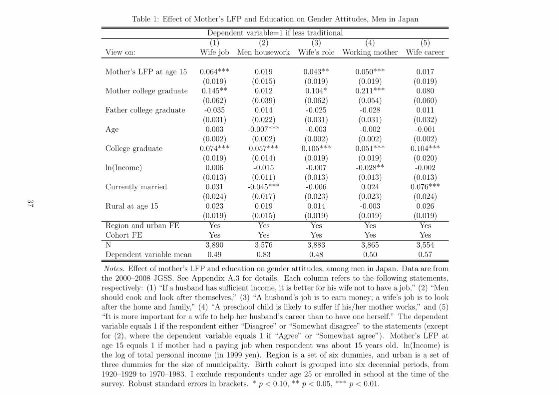
Table 1: Effect of Mother’s LFP and Education on Gender Attitudes, Men in Japan
Dependent variable=1 if less traditional(1) (2) (3) (4) (5)
View on: Wife job Men housework Wife’s role Working mother Wife career
Mother’s LFP at age 15 0.064*** 0.019 0.043** 0.050*** 0.017(0.019) (0.015) (0.019) (0.019) (0.019)
Mother college graduate 0.145** 0.012 0.104* 0.211*** 0.080(0.062) (0.039) (0.062) (0.054) (0.060)
Father college graduate -0.035 0.014 -0.025 -0.028 0.011(0.031) (0.022) (0.031) (0.031) (0.032)
Age 0.003 -0.007*** -0.003 -0.002 -0.001(0.002) (0.002) (0.002) (0.002) (0.002)
College graduate 0.074*** 0.057*** 0.105*** 0.051*** 0.104***(0.019) (0.014) (0.019) (0.019) (0.020)
ln(Income) 0.006 -0.015 -0.007 -0.028** -0.002(0.013) (0.011) (0.013) (0.013) (0.013)
Currently married 0.031 -0.045*** -0.006 0.024 0.076***(0.024) (0.017) (0.023) (0.023) (0.024)
Rural at age 15 0.023 0.019 0.014 -0.003 0.026(0.019) (0.015) (0.019) (0.019) (0.019)
Region and urban FE Yes Yes Yes Yes YesCohort FE Yes Yes Yes Yes YesN 3,890 3,576 3,883 3,865 3,554Dependent variable mean 0.49 0.83 0.48 0.50 0.57
Notes. Effect of mother’s LFP and education on gender attitudes, among men in Japan. Data are fromthe 2000–2008 JGSS. See Appendix A.3 for details. Each column refers to the following statements,respectively: (1) “If a husband has sufficient income, it is better for his wife not to have a job,” (2) “Menshould cook and look after themselves,” (3) “A husband’s job is to earn money; a wife’s job is to lookafter the home and family,” (4) “A preschool child is likely to suffer if his/her mother works,” and (5)“It is more important for a wife to help her husband’s career than to have one herself.” The dependentvariable equals 1 if the respondent either “Disagree” or “Somewhat disagree” to the statements (exceptfor (2), where the dependent variable equals 1 if “Agree” or “Somewhat agree”). Mother’s LFP atage 15 equals 1 if mother had a paying job when respondent was about 15 years old. ln(Income) isthe log of total personal income (in 1999 yen). Region is a set of six dummies, and urban is a set ofthree dummies for the size of municipality. Birth cohort is grouped into six decennial periods, from1920–1929 to 1970–1983. I exclude respondents under age 25 or enrolled in school at the time of thesurvey. Robust standard errors in brackets. * p < 0.10, ** p < 0.05, *** p < 0.01.
37
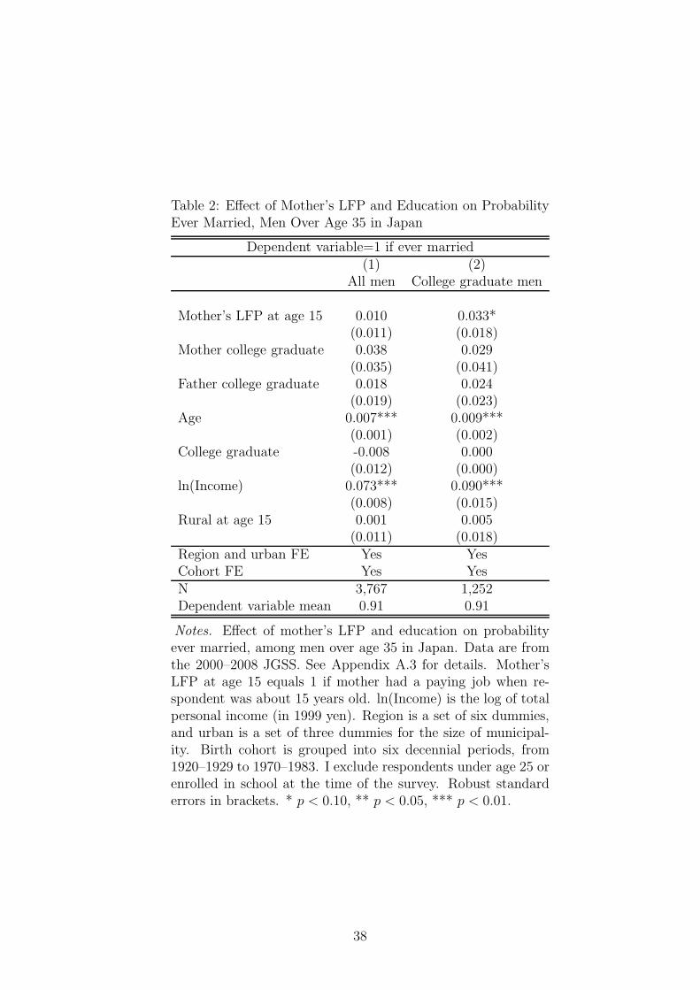
Table 2: Effect of Mother’s LFP and Education on ProbabilityEver Married, Men Over Age 35 in Japan
Dependent variable=1 if ever married(1) (2)
All men College graduate men
Mother’s LFP at age 15 0.010 0.033*(0.011) (0.018)
Mother college graduate 0.038 0.029(0.035) (0.041)
Father college graduate 0.018 0.024(0.019) (0.023)
Age 0.007*** 0.009***(0.001) (0.002)
College graduate -0.008 0.000(0.012) (0.000)
ln(Income) 0.073*** 0.090***(0.008) (0.015)
Rural at age 15 0.001 0.005(0.011) (0.018)
Region and urban FE Yes YesCohort FE Yes YesN 3,767 1,252Dependent variable mean 0.91 0.91
Notes. Effect of mother’s LFP and education on probabilityever married, among men over age 35 in Japan. Data are fromthe 2000–2008 JGSS. See Appendix A.3 for details. Mother’sLFP at age 15 equals 1 if mother had a paying job when re-spondent was about 15 years old. ln(Income) is the log of totalpersonal income (in 1999 yen). Region is a set of six dummies,and urban is a set of three dummies for the size of municipal-ity. Birth cohort is grouped into six decennial periods, from1920–1929 to 1970–1983. I exclude respondents under age 25 orenrolled in school at the time of the survey. Robust standarderrors in brackets. * p < 0.10, ** p < 0.05, *** p < 0.01.
38
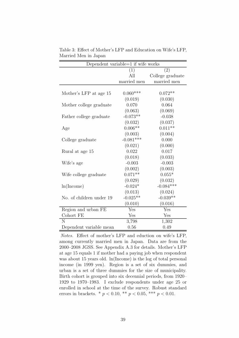
Table 3: Effect of Mother’s LFP and Education on Wife’s LFP,Married Men in Japan
Dependent variable=1 if wife works(1) (2)All College graduate
married men married men
Mother’s LFP at age 15 0.060*** 0.072**(0.019) (0.030)
Mother college graduate 0.070 0.064(0.063) (0.069)
Father college graduate -0.073** -0.038(0.032) (0.037)
Age 0.006** 0.011**(0.003) (0.004)
College graduate -0.081*** 0.000(0.021) (0.000)
Rural at age 15 0.022 0.017(0.018) (0.033)
Wife’s age -0.003 -0.003(0.002) (0.003)
Wife college graduate 0.071** 0.055*(0.029) (0.032)
ln(Income) -0.024* -0.084***(0.013) (0.024)
No. of children under 19 -0.025** -0.039**(0.010) (0.016)
Region and urban FE Yes YesCohort FE Yes YesN 3,798 1,302Dependent variable mean 0.56 0.49
Notes. Effect of mother’s LFP and eduction on wife’s LFP,among currently married men in Japan. Data are from the2000–2008 JGSS. See Appendix A.3 for details. Mother’s LFPat age 15 equals 1 if mother had a paying job when respondentwas about 15 years old. ln(Income) is the log of total personalincome (in 1999 yen). Region is a set of six dummies, andurban is a set of three dummies for the size of municipality.Birth cohort is grouped into six decennial periods, from 1920–1929 to 1970–1983. I exclude respondents under age 25 orenrolled in school at the time of the survey. Robust standarderrors in brackets. * p < 0.10, ** p < 0.05, *** p < 0.01.
39
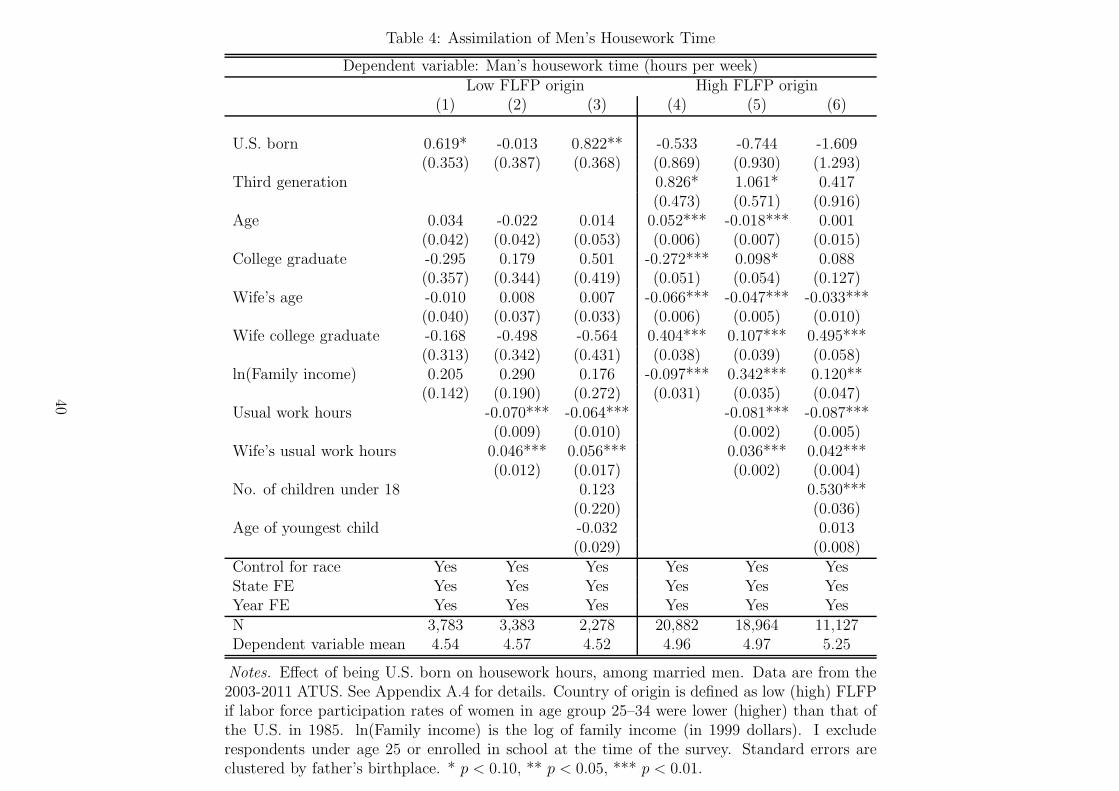
Table 4: Assimilation of Men’s Housework Time
Dependent variable: Man’s housework time (hours per week)Low FLFP origin High FLFP origin
(1) (2) (3) (4) (5) (6)
U.S. born 0.619* -0.013 0.822** -0.533 -0.744 -1.609(0.353) (0.387) (0.368) (0.869) (0.930) (1.293)
Third generation 0.826* 1.061* 0.417(0.473) (0.571) (0.916)
Age 0.034 -0.022 0.014 0.052*** -0.018*** 0.001(0.042) (0.042) (0.053) (0.006) (0.007) (0.015)
College graduate -0.295 0.179 0.501 -0.272*** 0.098* 0.088(0.357) (0.344) (0.419) (0.051) (0.054) (0.127)
Wife’s age -0.010 0.008 0.007 -0.066*** -0.047*** -0.033***(0.040) (0.037) (0.033) (0.006) (0.005) (0.010)
Wife college graduate -0.168 -0.498 -0.564 0.404*** 0.107*** 0.495***(0.313) (0.342) (0.431) (0.038) (0.039) (0.058)
ln(Family income) 0.205 0.290 0.176 -0.097*** 0.342*** 0.120**(0.142) (0.190) (0.272) (0.031) (0.035) (0.047)
Usual work hours -0.070*** -0.064*** -0.081*** -0.087***(0.009) (0.010) (0.002) (0.005)
Wife’s usual work hours 0.046*** 0.056*** 0.036*** 0.042***(0.012) (0.017) (0.002) (0.004)
No. of children under 18 0.123 0.530***(0.220) (0.036)
Age of youngest child -0.032 0.013(0.029) (0.008)
Control for race Yes Yes Yes Yes Yes YesState FE Yes Yes Yes Yes Yes YesYear FE Yes Yes Yes Yes Yes YesN 3,783 3,383 2,278 20,882 18,964 11,127Dependent variable mean 4.54 4.57 4.52 4.96 4.97 5.25
Notes. Effect of being U.S. born on housework hours, among married men. Data are from the2003-2011 ATUS. See Appendix A.4 for details. Country of origin is defined as low (high) FLFPif labor force participation rates of women in age group 25–34 were lower (higher) than that ofthe U.S. in 1985. ln(Family income) is the log of family income (in 1999 dollars). I excluderespondents under age 25 or enrolled in school at the time of the survey. Standard errors areclustered by father’s birthplace. * p < 0.10, ** p < 0.05, *** p < 0.01.
40
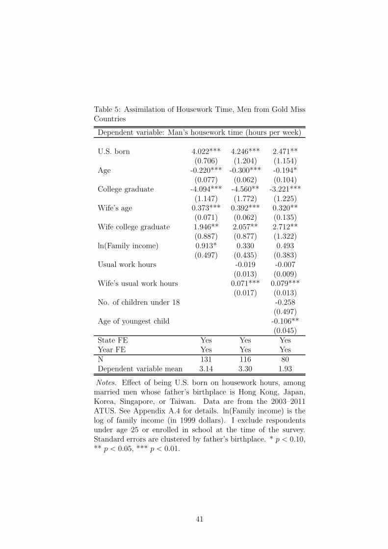
Table 5: Assimilation of Housework Time, Men from Gold MissCountries
Dependent variable: Man’s housework time (hours per week)
U.S. born 4.022*** 4.246*** 2.471**(0.706) (1.204) (1.154)
Age -0.220*** -0.300*** -0.194*(0.077) (0.062) (0.104)
College graduate -4.094*** -4.560** -3.221***(1.147) (1.772) (1.225)
Wife’s age 0.373*** 0.392*** 0.320**(0.071) (0.062) (0.135)
Wife college graduate 1.946** 2.057** 2.712**(0.887) (0.877) (1.322)
ln(Family income) 0.913* 0.330 0.493(0.497) (0.435) (0.383)
Usual work hours -0.019 -0.007(0.013) (0.009)
Wife’s usual work hours 0.071*** 0.079***(0.017) (0.013)
No. of children under 18 -0.258(0.497)
Age of youngest child -0.106**(0.045)
State FE Yes Yes YesYear FE Yes Yes YesN 131 116 80Dependent variable mean 3.14 3.30 1.93
Notes. Effect of being U.S. born on housework hours, amongmarried men whose father’s birthplace is Hong Kong, Japan,Korea, Singapore, or Taiwan. Data are from the 2003–2011ATUS. See Appendix A.4 for details. ln(Family income) is thelog of family income (in 1999 dollars). I exclude respondentsunder age 25 or enrolled in school at the time of the survey.Standard errors are clustered by father’s birthplace. * p < 0.10,** p < 0.05, *** p < 0.01.
41
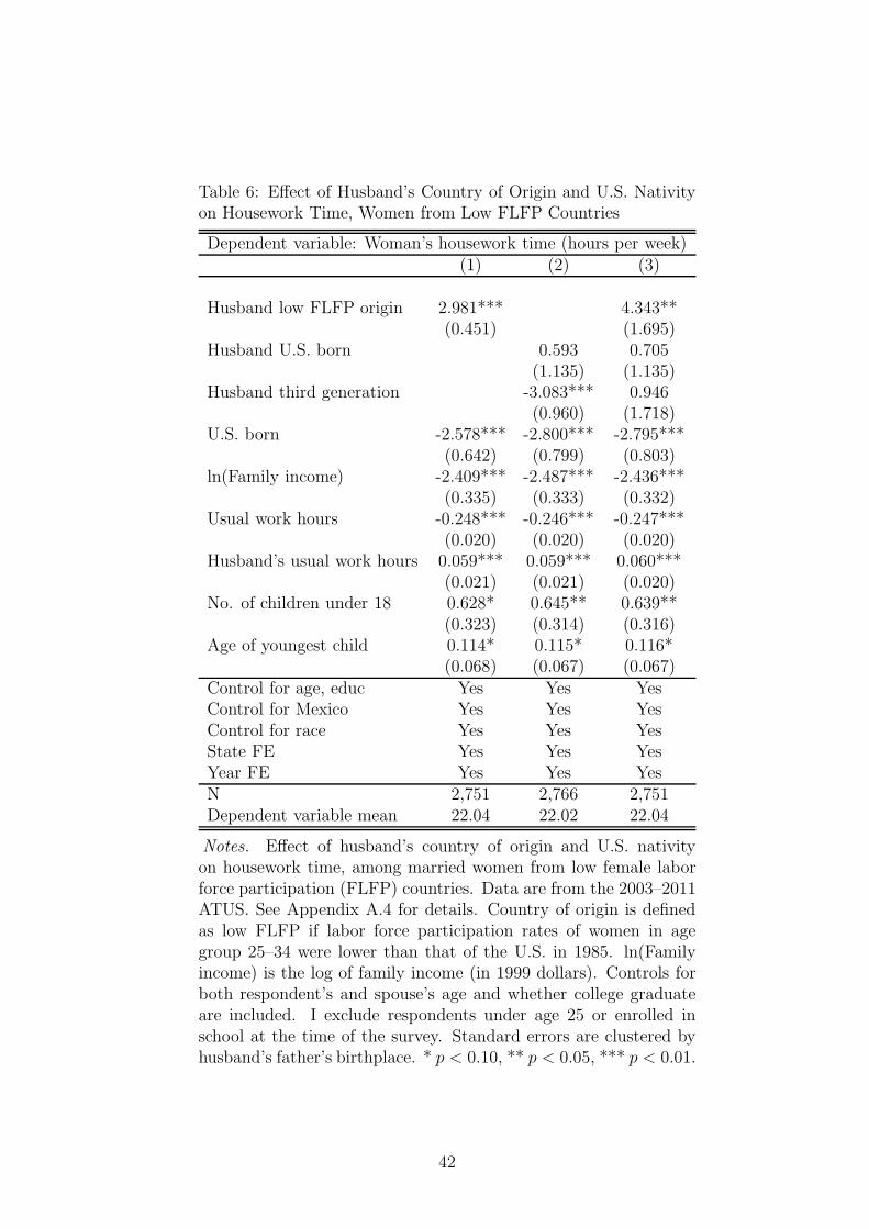
Table 6: Effect of Husband’s Country of Origin and U.S. Nativityon Housework Time, Women from Low FLFP Countries
Dependent variable: Woman’s housework time (hours per week)(1) (2) (3)
Husband low FLFP origin 2.981*** 4.343**(0.451) (1.695)
Husband U.S. born 0.593 0.705(1.135) (1.135)
Husband third generation -3.083*** 0.946(0.960) (1.718)
U.S. born -2.578*** -2.800*** -2.795***(0.642) (0.799) (0.803)
ln(Family income) -2.409*** -2.487*** -2.436***(0.335) (0.333) (0.332)
Usual work hours -0.248*** -0.246*** -0.247***(0.020) (0.020) (0.020)
Husband’s usual work hours 0.059*** 0.059*** 0.060***(0.021) (0.021) (0.020)
No. of children under 18 0.628* 0.645** 0.639**(0.323) (0.314) (0.316)
Age of youngest child 0.114* 0.115* 0.116*(0.068) (0.067) (0.067)
Control for age, educ Yes Yes YesControl for Mexico Yes Yes YesControl for race Yes Yes YesState FE Yes Yes YesYear FE Yes Yes YesN 2,751 2,766 2,751Dependent variable mean 22.04 22.02 22.04
Notes. Effect of husband’s country of origin and U.S. nativityon housework time, among married women from low female laborforce participation (FLFP) countries. Data are from the 2003–2011ATUS. See Appendix A.4 for details. Country of origin is definedas low FLFP if labor force participation rates of women in agegroup 25–34 were lower than that of the U.S. in 1985. ln(Familyincome) is the log of family income (in 1999 dollars). Controls forboth respondent’s and spouse’s age and whether college graduateare included. I exclude respondents under age 25 or enrolled inschool at the time of the survey. Standard errors are clustered byhusband’s father’s birthplace. * p < 0.10, ** p < 0.05, *** p < 0.01.
42
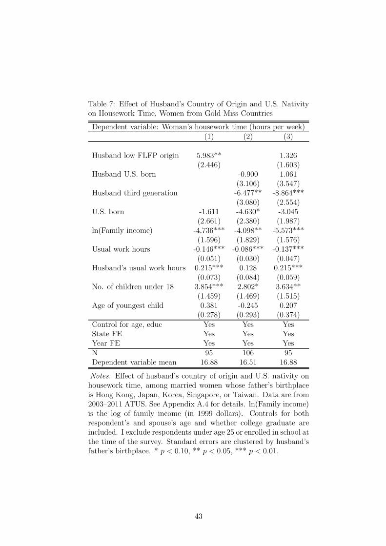
Table 7: Effect of Husband’s Country of Origin and U.S. Nativityon Housework Time, Women from Gold Miss Countries
Dependent variable: Woman’s housework time (hours per week)(1) (2) (3)
Husband low FLFP origin 5.983** 1.326(2.446) (1.603)
Husband U.S. born -0.900 1.061(3.106) (3.547)
Husband third generation -6.477** -8.864***(3.080) (2.554)
U.S. born -1.611 -4.630* -3.045(2.661) (2.380) (1.987)
ln(Family income) -4.736*** -4.098** -5.573***(1.596) (1.829) (1.576)
Usual work hours -0.146*** -0.086*** -0.137***(0.051) (0.030) (0.047)
Husband’s usual work hours 0.215*** 0.128 0.215***(0.073) (0.084) (0.059)
No. of children under 18 3.854*** 2.802* 3.634**(1.459) (1.469) (1.515)
Age of youngest child 0.381 -0.245 0.207(0.278) (0.293) (0.374)
Control for age, educ Yes Yes YesState FE Yes Yes YesYear FE Yes Yes YesN 95 106 95Dependent variable mean 16.88 16.51 16.88
Notes. Effect of husband’s country of origin and U.S. nativity onhousework time, among married women whose father’s birthplaceis Hong Kong, Japan, Korea, Singapore, or Taiwan. Data are from2003–2011 ATUS. See Appendix A.4 for details. ln(Family income)is the log of family income (in 1999 dollars). Controls for bothrespondent’s and spouse’s age and whether college graduate areincluded. I exclude respondents under age 25 or enrolled in school atthe time of the survey. Standard errors are clustered by husband’sfather’s birthplace. * p < 0.10, ** p < 0.05, *** p < 0.01.
43
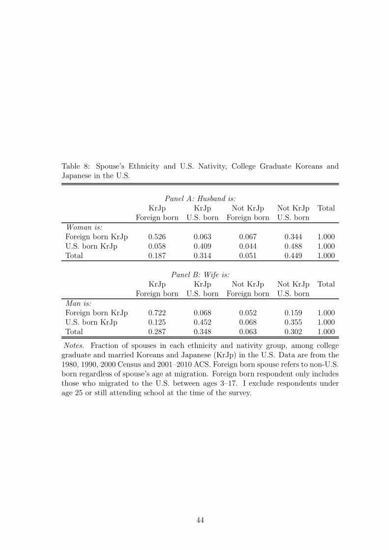
Table 8: Spouse’s Ethnicity and U.S. Nativity, College Graduate Koreans andJapanese in the U.S.
Panel A: Husband is:KrJp KrJp Not KrJp Not KrJp Total
Foreign born U.S. born Foreign born U.S. bornWoman is:Foreign born KrJp 0.526 0.063 0.067 0.344 1.000U.S. born KrJp 0.058 0.409 0.044 0.488 1.000Total 0.187 0.314 0.051 0.449 1.000
Panel B: Wife is:KrJp KrJp Not KrJp Not KrJp Total
Foreign born U.S. born Foreign born U.S. bornMan is:Foreign born KrJp 0.722 0.068 0.052 0.159 1.000U.S. born KrJp 0.125 0.452 0.068 0.355 1.000Total 0.287 0.348 0.063 0.302 1.000
Notes. Fraction of spouses in each ethnicity and nativity group, among collegegraduate and married Koreans and Japanese (KrJp) in the U.S. Data are from the1980, 1990, 2000 Census and 2001–2010 ACS. Foreign born spouse refers to non-U.S.born regardless of spouse’s age at migration. Foreign born respondent only includesthose who migrated to the U.S. between ages 3–17. I exclude respondents underage 25 or still attending school at the time of the survey.
44
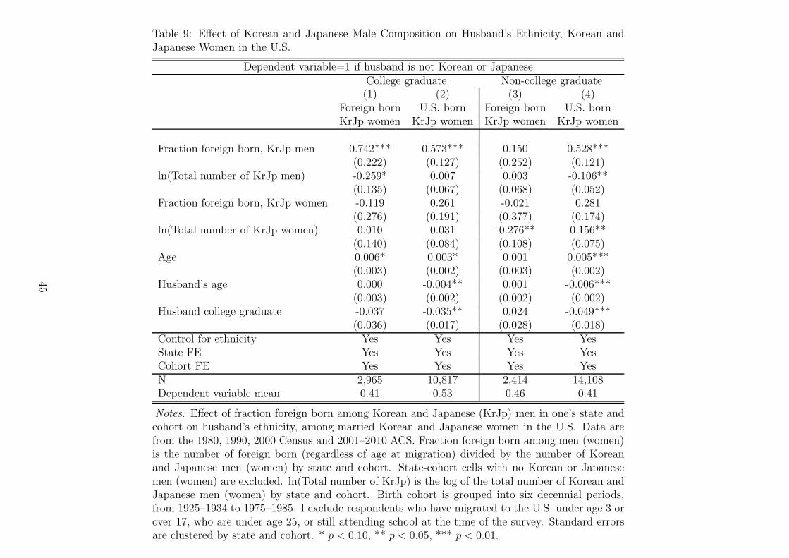
Table 9: Effect of Korean and Japanese Male Composition on Husband’s Ethnicity, Korean andJapanese Women in the U.S.
Dependent variable=1 if husband is not Korean or JapaneseCollege graduate Non-college graduate(1) (2) (3) (4)
Foreign born U.S. born Foreign born U.S. bornKrJp women KrJp women KrJp women KrJp women
Fraction foreign born, KrJp men 0.742*** 0.573*** 0.150 0.528***(0.222) (0.127) (0.252) (0.121)
ln(Total number of KrJp men) -0.259* 0.007 0.003 -0.106**(0.135) (0.067) (0.068) (0.052)
Fraction foreign born, KrJp women -0.119 0.261 -0.021 0.281(0.276) (0.191) (0.377) (0.174)
ln(Total number of KrJp women) 0.010 0.031 -0.276** 0.156**(0.140) (0.084) (0.108) (0.075)
Age 0.006* 0.003* 0.001 0.005***(0.003) (0.002) (0.003) (0.002)
Husband’s age 0.000 -0.004** 0.001 -0.006***(0.003) (0.002) (0.002) (0.002)
Husband college graduate -0.037 -0.035** 0.024 -0.049***(0.036) (0.017) (0.028) (0.018)
Control for ethnicity Yes Yes Yes YesState FE Yes Yes Yes YesCohort FE Yes Yes Yes YesN 2,965 10,817 2,414 14,108Dependent variable mean 0.41 0.53 0.46 0.41
Notes. Effect of fraction foreign born among Korean and Japanese (KrJp) men in one’s state andcohort on husband’s ethnicity, among married Korean and Japanese women in the U.S. Data arefrom the 1980, 1990, 2000 Census and 2001–2010 ACS. Fraction foreign born among men (women)is the number of foreign born (regardless of age at migration) divided by the number of Koreanand Japanese men (women) by state and cohort. State-cohort cells with no Korean or Japanesemen (women) are excluded. ln(Total number of KrJp) is the log of the total number of Korean andJapanese men (women) by state and cohort. Birth cohort is grouped into six decennial periods,from 1925–1934 to 1975–1985. I exclude respondents who have migrated to the U.S. under age 3 orover 17, who are under age 25, or still attending school at the time of the survey. Standard errorsare clustered by state and cohort. * p < 0.10, ** p < 0.05, *** p < 0.01.
45
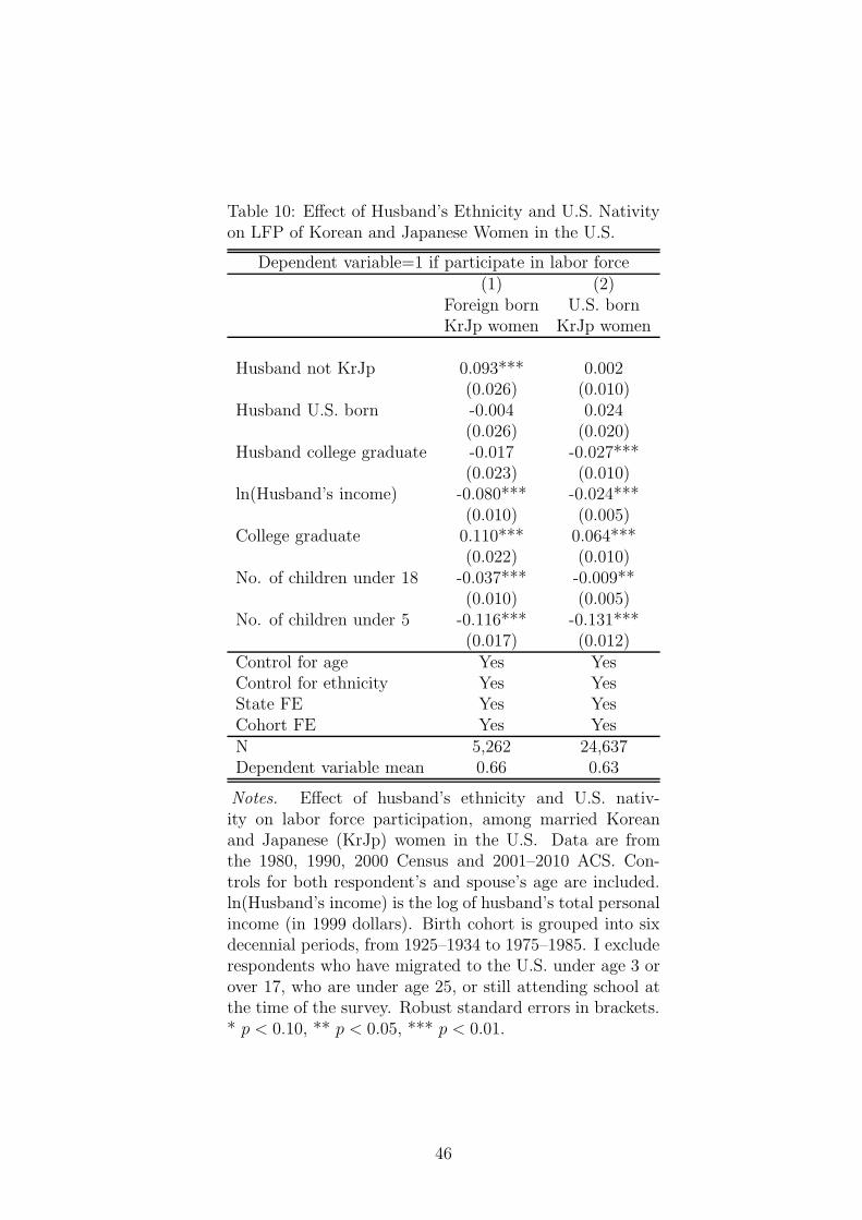
Table 10: Effect of Husband’s Ethnicity and U.S. Nativityon LFP of Korean and Japanese Women in the U.S.
Dependent variable=1 if participate in labor force(1) (2)
Foreign born U.S. bornKrJp women KrJp women
Husband not KrJp 0.093*** 0.002(0.026) (0.010)
Husband U.S. born -0.004 0.024(0.026) (0.020)
Husband college graduate -0.017 -0.027***(0.023) (0.010)
ln(Husband’s income) -0.080*** -0.024***(0.010) (0.005)
College graduate 0.110*** 0.064***(0.022) (0.010)
No. of children under 18 -0.037*** -0.009**(0.010) (0.005)
No. of children under 5 -0.116*** -0.131***(0.017) (0.012)
Control for age Yes YesControl for ethnicity Yes YesState FE Yes YesCohort FE Yes YesN 5,262 24,637Dependent variable mean 0.66 0.63
Notes. Effect of husband’s ethnicity and U.S. nativ-ity on labor force participation, among married Koreanand Japanese (KrJp) women in the U.S. Data are fromthe 1980, 1990, 2000 Census and 2001–2010 ACS. Con-trols for both respondent’s and spouse’s age are included.ln(Husband’s income) is the log of husband’s total personalincome (in 1999 dollars). Birth cohort is grouped into sixdecennial periods, from 1925–1934 to 1975–1985. I excluderespondents who have migrated to the U.S. under age 3 orover 17, who are under age 25, or still attending school atthe time of the survey. Robust standard errors in brackets.* p < 0.10, ** p < 0.05, *** p < 0.01.
46
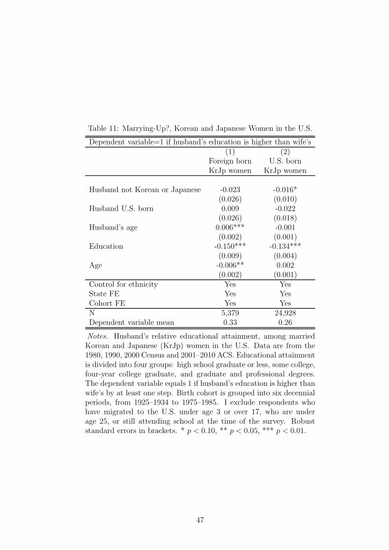
Table 11: Marrying-Up?, Korean and Japanese Women in the U.S.
Dependent variable=1 if husband’s education is higher than wife’s(1) (2)
Foreign born U.S. bornKrJp women KrJp women
Husband not Korean or Japanese -0.023 -0.016*(0.026) (0.010)
Husband U.S. born 0.009 -0.022(0.026) (0.018)
Husband’s age 0.006*** -0.001(0.002) (0.001)
Education -0.150*** -0.134***(0.009) (0.004)
Age -0.006** 0.002(0.002) (0.001)
Control for ethnicity Yes YesState FE Yes YesCohort FE Yes YesN 5,379 24,928Dependent variable mean 0.33 0.26
Notes. Husband’s relative educational attainment, among marriedKorean and Japanese (KrJp) women in the U.S. Data are from the1980, 1990, 2000 Census and 2001–2010 ACS. Educational attainmentis divided into four groups: high school graduate or less, some college,four-year college graduate, and graduate and professional degrees.The dependent variable equals 1 if husband’s education is higher thanwife’s by at least one step. Birth cohort is grouped into six decennialperiods, from 1925–1934 to 1975–1985. I exclude respondents whohave migrated to the U.S. under age 3 or over 17, who are underage 25, or still attending school at the time of the survey. Robuststandard errors in brackets. * p < 0.10, ** p < 0.05, *** p < 0.01.
47
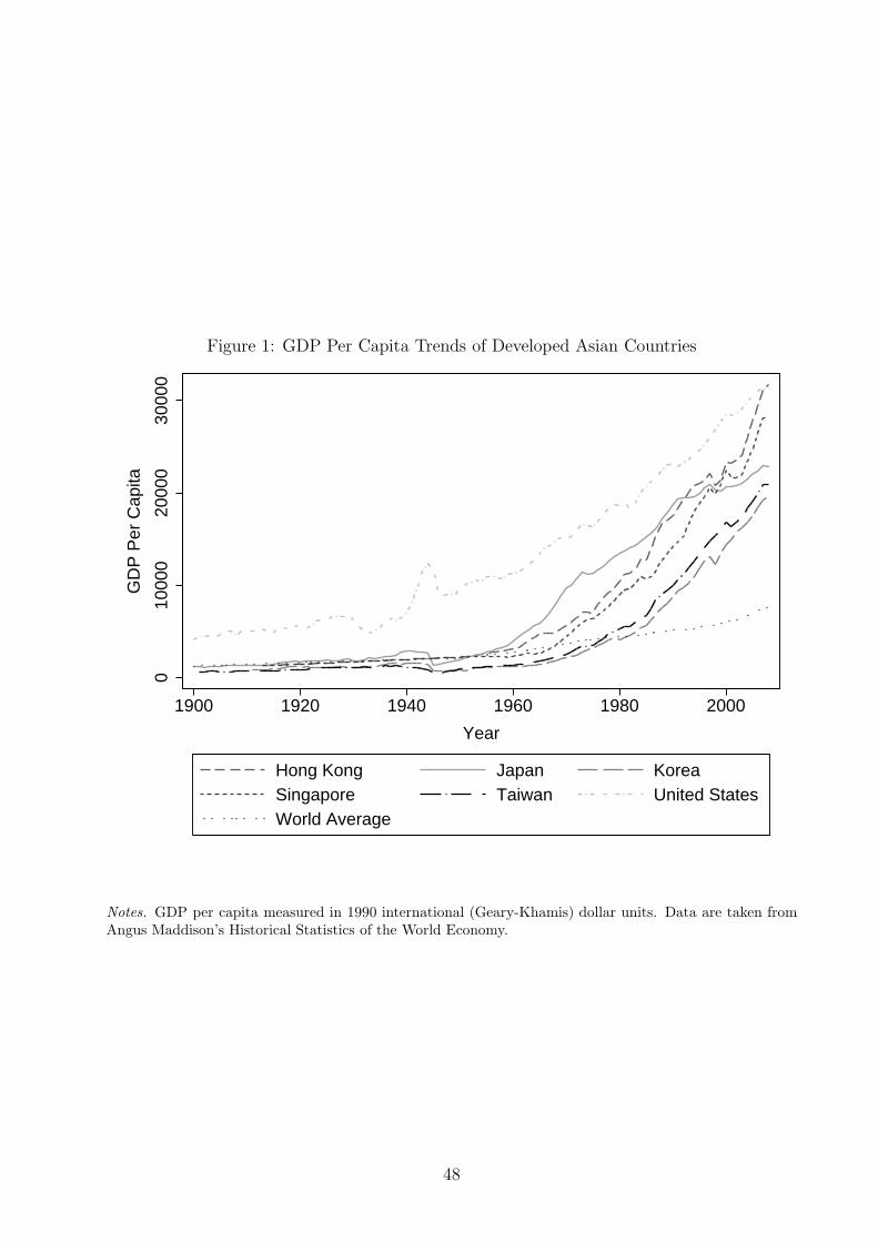
Figure 1: GDP Per Capita Trends of Developed Asian Countries
010
000
2000
030
000
GD
P P
er C
apita
1900 1920 1940 1960 1980 2000
Year
Hong Kong Japan KoreaSingapore Taiwan United StatesWorld Average
Notes. GDP per capita measured in 1990 international (Geary-Khamis) dollar units. Data are taken fromAngus Maddison’s Historical Statistics of the World Economy.
48
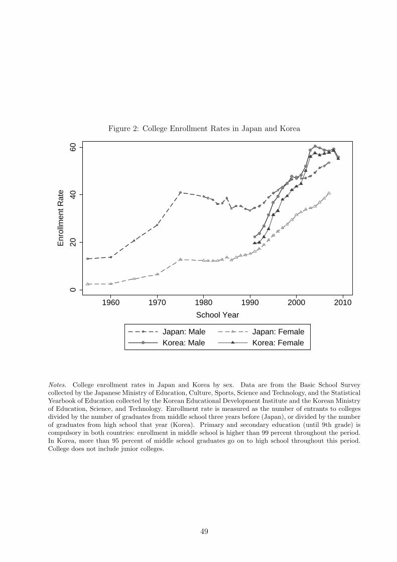
Figure 2: College Enrollment Rates in Japan and Korea
020
4060
Enr
ollm
ent R
ate
1960 1970 1980 1990 2000 2010
School Year
Japan: Male Japan: FemaleKorea: Male Korea: Female
Notes. College enrollment rates in Japan and Korea by sex. Data are from the Basic School Surveycollected by the Japanese Ministry of Education, Culture, Sports, Science and Technology, and the StatisticalYearbook of Education collected by the Korean Educational Development Institute and the Korean Ministryof Education, Science, and Technology. Enrollment rate is measured as the number of entrants to collegesdivided by the number of graduates from middle school three years before (Japan), or divided by the numberof graduates from high school that year (Korea). Primary and secondary education (until 9th grade) iscompulsory in both countries: enrollment in middle school is higher than 99 percent throughout the period.In Korea, more than 95 percent of middle school graduates go on to high school throughout this period.College does not include junior colleges.
49
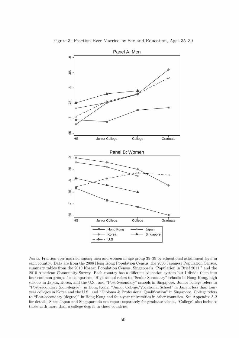
Figure 3: Fraction Ever Married by Sex and Education, Ages 35–39
.65
.7.7
5.8
.85
.9
HS Junior College College Graduate
Panel A: Men
.65
.7.7
5.8
.85
.9
HS Junior College College Graduate
Hong Kong Japan
Korea Singapore
U.S
Panel B: Women
Notes. Fraction ever married among men and women in age group 35–39 by educational attainment level ineach country. Data are from the 2006 Hong Kong Population Census, the 2000 Japanese Population Census,summary tables from the 2010 Korean Population Census, Singapore’s “Population in Brief 2011,” and the2010 American Community Survey. Each country has a different education system but I divide them intofour common groups for comparison. High school refers to “Senior Secondary” schools in Hong Kong, highschools in Japan, Korea, and the U.S., and “Post-Secondary” schools in Singapore. Junior college refers to“Post-secondary (non-degree)” in Hong Kong, “Junior College/Vocational School” in Japan, less than four-year colleges in Korea and the U.S., and “Diploma & Professional Qualification” in Singapore. College refersto “Post-secondary (degree)” in Hong Kong and four-year universities in other countries. See Appendix A.2for details. Since Japan and Singapore do not report separately for graduate school, “College” also includesthose with more than a college degree in these countries.
50
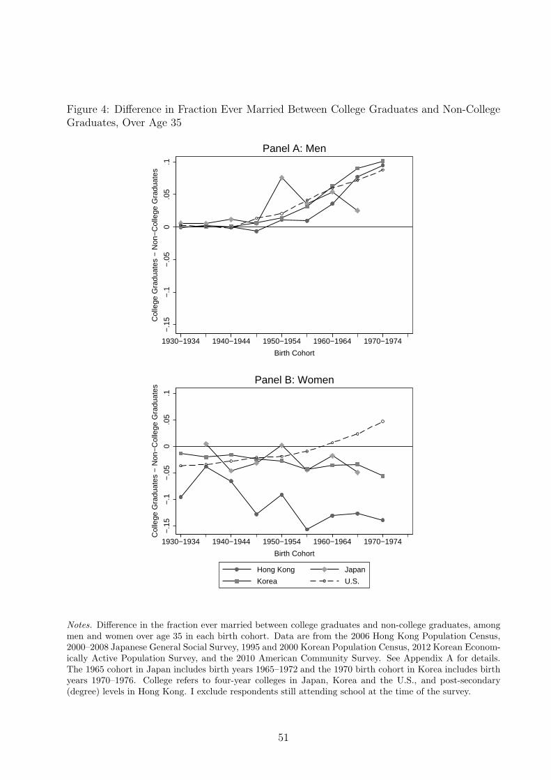
Figure 4: Difference in Fraction Ever Married Between College Graduates and Non-CollegeGraduates, Over Age 35
−.1
5−
.1−
.05
0.0
5.1
Col
lege
Gra
duat
es −
Non
−C
olle
ge G
radu
ates
1930−1934 1940−1944 1950−1954 1960−1964 1970−1974
Birth Cohort
Panel A: Men
−.1
5−
.1−
.05
0.0
5.1
Col
lege
Gra
duat
es −
Non
−C
olle
ge G
radu
ates
1930−1934 1940−1944 1950−1954 1960−1964 1970−1974
Birth Cohort
Hong Kong Japan
Korea U.S.
Panel B: Women
Notes. Difference in the fraction ever married between college graduates and non-college graduates, amongmen and women over age 35 in each birth cohort. Data are from the 2006 Hong Kong Population Census,2000–2008 Japanese General Social Survey, 1995 and 2000 Korean Population Census, 2012 Korean Econom-ically Active Population Survey, and the 2010 American Community Survey. See Appendix A for details.The 1965 cohort in Japan includes birth years 1965–1972 and the 1970 birth cohort in Korea includes birthyears 1970–1976. College refers to four-year colleges in Japan, Korea and the U.S., and post-secondary(degree) levels in Hong Kong. I exclude respondents still attending school at the time of the survey.
51
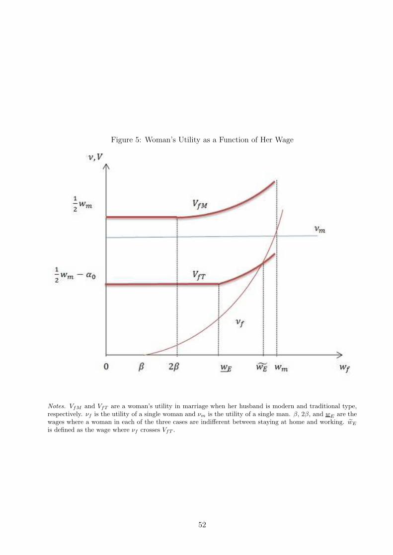
Figure 5: Woman’s Utility as a Function of Her Wage
Notes. VfM and VfT are a woman’s utility in marriage when her husband is modern and traditional type,respectively. νf is the utility of a single woman and νm is the utility of a single man. β, 2β, and wE are thewages where a woman in each of the three cases are indifferent between staying at home and working. wE
is defined as the wage where νf crosses VfT .
52
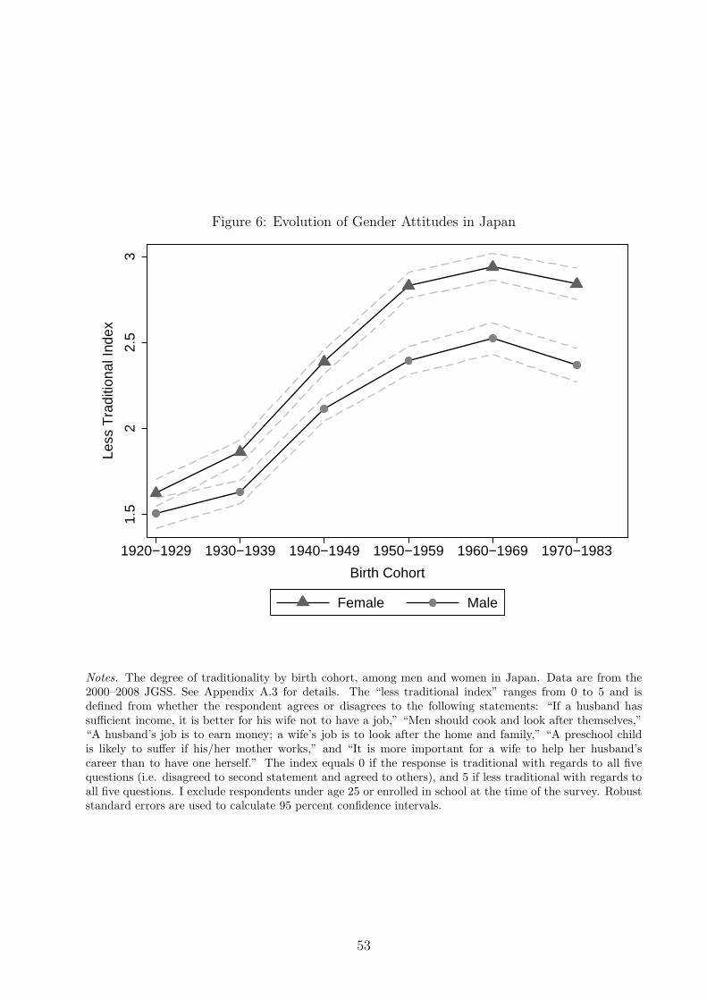
Figure 6: Evolution of Gender Attitudes in Japan
1.5
22.
53
Less
Tra
ditio
nal I
ndex
1920−1929 1930−1939 1940−1949 1950−1959 1960−1969 1970−1983
Birth Cohort
Female Male
Notes. The degree of traditionality by birth cohort, among men and women in Japan. Data are from the2000–2008 JGSS. See Appendix A.3 for details. The “less traditional index” ranges from 0 to 5 and isdefined from whether the respondent agrees or disagrees to the following statements: “If a husband hassufficient income, it is better for his wife not to have a job,” “Men should cook and look after themselves,”“A husband’s job is to earn money; a wife’s job is to look after the home and family,” “A preschool childis likely to suffer if his/her mother works,” and “It is more important for a wife to help her husband’scareer than to have one herself.” The index equals 0 if the response is traditional with regards to all fivequestions (i.e. disagreed to second statement and agreed to others), and 5 if less traditional with regards toall five questions. I exclude respondents under age 25 or enrolled in school at the time of the survey. Robuststandard errors are used to calculate 95 percent confidence intervals.
53
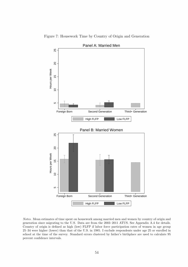
Figure 7: Housework Time by Country of Origin and Generation
510
1520
25
Hou
rs p
er W
eek
Foreign Born Second Generation Third+ Generation
High FLFP Low FLFP
Panel A: Married Men
510
1520
25
Hou
rs p
er W
eek
Foreign Born Second Generation Third+ Generation
High FLFP Low FLFP
Panel B: Married Women
Notes. Mean estimates of time spent on housework among married men and women by country of origin andgeneration since migrating to the U.S. Data are from the 2003–2011 ATUS. See Appendix A.4 for details.Country of origin is defined as high (low) FLFP if labor force participation rates of women in age group25–34 were higher (lower) than that of the U.S. in 1985. I exclude respondents under age 25 or enrolled inschool at the time of the survey. Standard errors clustered by father’s birthplace are used to calculate 95percent confidence intervals.
54
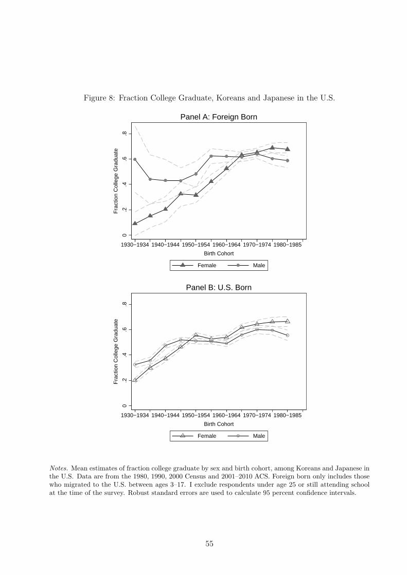
Figure 8: Fraction College Graduate, Koreans and Japanese in the U.S.
0.2
.4.6
.8
Fra
ctio
n C
olle
ge G
radu
ate
1930−1934 1940−1944 1950−1954 1960−1964 1970−1974 1980−1985
Birth Cohort
Female Male
Panel A: Foreign Born0
.2.4
.6.8
Fra
ctio
n C
olle
ge G
radu
ate
1930−1934 1940−1944 1950−1954 1960−1964 1970−1974 1980−1985
Birth Cohort
Female Male
Panel B: U.S. Born
Notes. Mean estimates of fraction college graduate by sex and birth cohort, among Koreans and Japanese inthe U.S. Data are from the 1980, 1990, 2000 Census and 2001–2010 ACS. Foreign born only includes thosewho migrated to the U.S. between ages 3–17. I exclude respondents under age 25 or still attending schoolat the time of the survey. Robust standard errors are used to calculate 95 percent confidence intervals.
55
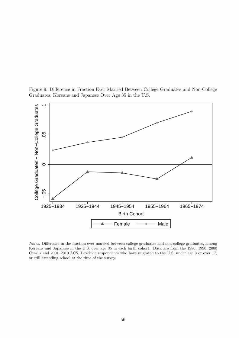
Figure 9: Difference in Fraction Ever Married Between College Graduates and Non-CollegeGraduates, Koreans and Japanese Over Age 35 in the U.S.
−.0
50
.05
.1
Col
lege
Gra
duat
es −
Non
−C
olle
ge G
radu
ates
1925−1934 1935−1944 1945−1954 1955−1964 1965−1974
Birth Cohort
Female Male
Notes. Difference in the fraction ever married between college graduates and non-college graduates, amongKoreans and Japanese in the U.S. over age 35 in each birth cohort. Data are from the 1980, 1990, 2000Census and 2001–2010 ACS. I exclude respondents who have migrated to the U.S. under age 3 or over 17,or still attending school at the time of the survey.
56
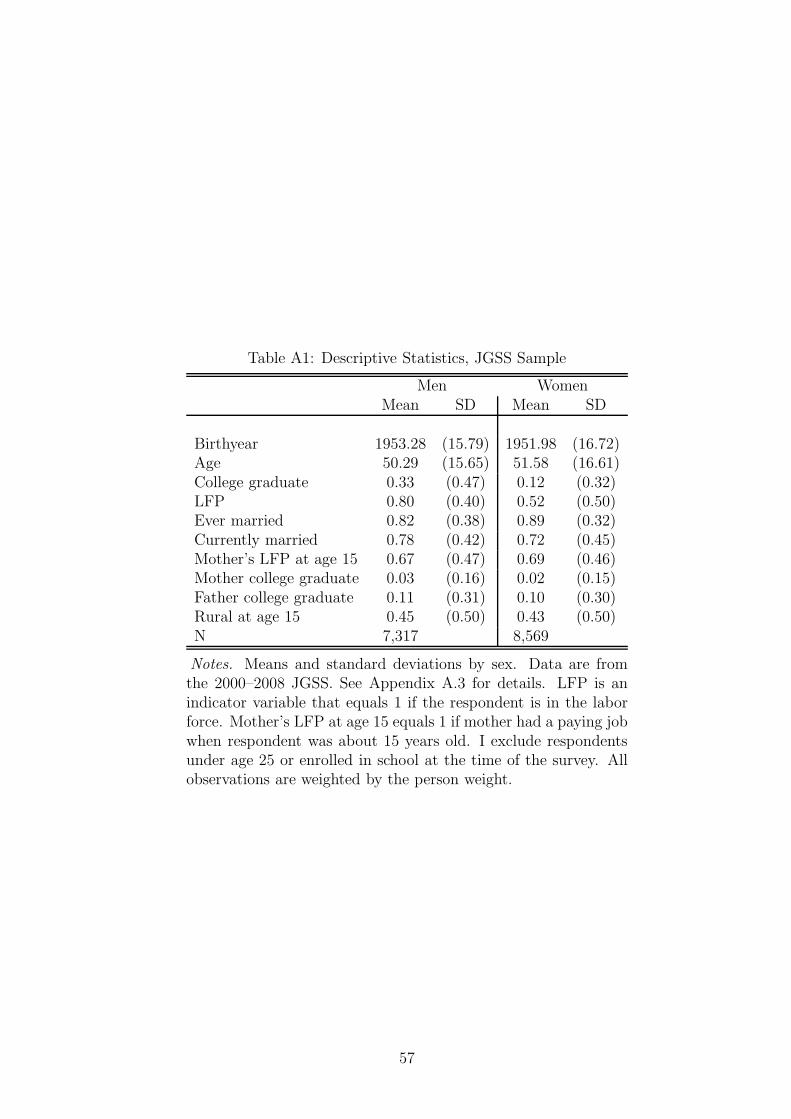
Table A1: Descriptive Statistics, JGSS Sample
Men WomenMean SD Mean SD
Birthyear 1953.28 (15.79) 1951.98 (16.72)Age 50.29 (15.65) 51.58 (16.61)College graduate 0.33 (0.47) 0.12 (0.32)LFP 0.80 (0.40) 0.52 (0.50)Ever married 0.82 (0.38) 0.89 (0.32)Currently married 0.78 (0.42) 0.72 (0.45)Mother’s LFP at age 15 0.67 (0.47) 0.69 (0.46)Mother college graduate 0.03 (0.16) 0.02 (0.15)Father college graduate 0.11 (0.31) 0.10 (0.30)Rural at age 15 0.45 (0.50) 0.43 (0.50)N 7,317 8,569
Notes. Means and standard deviations by sex. Data are fromthe 2000–2008 JGSS. See Appendix A.3 for details. LFP is anindicator variable that equals 1 if the respondent is in the laborforce. Mother’s LFP at age 15 equals 1 if mother had a paying jobwhen respondent was about 15 years old. I exclude respondentsunder age 25 or enrolled in school at the time of the survey. Allobservations are weighted by the person weight.
57
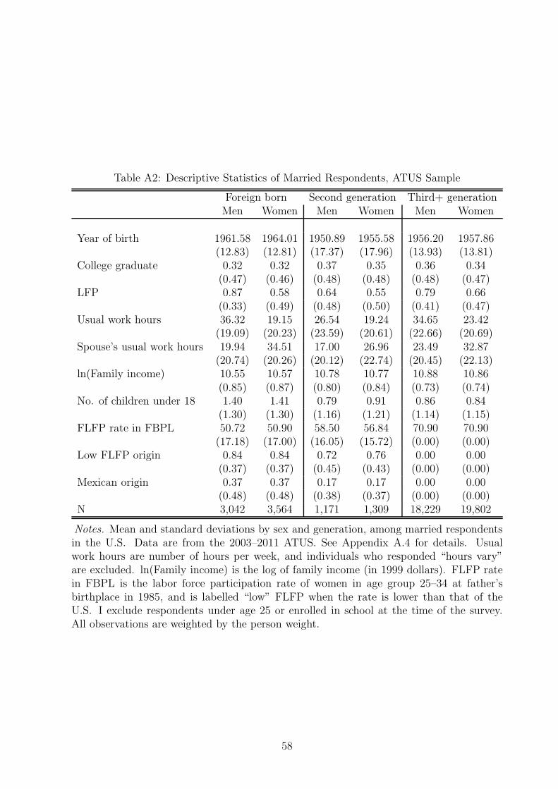
Table A2: Descriptive Statistics of Married Respondents, ATUS Sample
Foreign born Second generation Third+ generationMen Women Men Women Men Women
Year of birth 1961.58 1964.01 1950.89 1955.58 1956.20 1957.86(12.83) (12.81) (17.37) (17.96) (13.93) (13.81)
College graduate 0.32 0.32 0.37 0.35 0.36 0.34(0.47) (0.46) (0.48) (0.48) (0.48) (0.47)
LFP 0.87 0.58 0.64 0.55 0.79 0.66(0.33) (0.49) (0.48) (0.50) (0.41) (0.47)
Usual work hours 36.32 19.15 26.54 19.24 34.65 23.42(19.09) (20.23) (23.59) (20.61) (22.66) (20.69)
Spouse’s usual work hours 19.94 34.51 17.00 26.96 23.49 32.87(20.74) (20.26) (20.12) (22.74) (20.45) (22.13)
ln(Family income) 10.55 10.57 10.78 10.77 10.88 10.86(0.85) (0.87) (0.80) (0.84) (0.73) (0.74)
No. of children under 18 1.40 1.41 0.79 0.91 0.86 0.84(1.30) (1.30) (1.16) (1.21) (1.14) (1.15)
FLFP rate in FBPL 50.72 50.90 58.50 56.84 70.90 70.90(17.18) (17.00) (16.05) (15.72) (0.00) (0.00)
Low FLFP origin 0.84 0.84 0.72 0.76 0.00 0.00(0.37) (0.37) (0.45) (0.43) (0.00) (0.00)
Mexican origin 0.37 0.37 0.17 0.17 0.00 0.00(0.48) (0.48) (0.38) (0.37) (0.00) (0.00)
N 3,042 3,564 1,171 1,309 18,229 19,802
Notes. Mean and standard deviations by sex and generation, among married respondentsin the U.S. Data are from the 2003–2011 ATUS. See Appendix A.4 for details. Usualwork hours are number of hours per week, and individuals who responded “hours vary”are excluded. ln(Family income) is the log of family income (in 1999 dollars). FLFP ratein FBPL is the labor force participation rate of women in age group 25–34 at father’sbirthplace in 1985, and is labelled “low” FLFP when the rate is lower than that of theU.S. I exclude respondents under age 25 or enrolled in school at the time of the survey.All observations are weighted by the person weight.
58
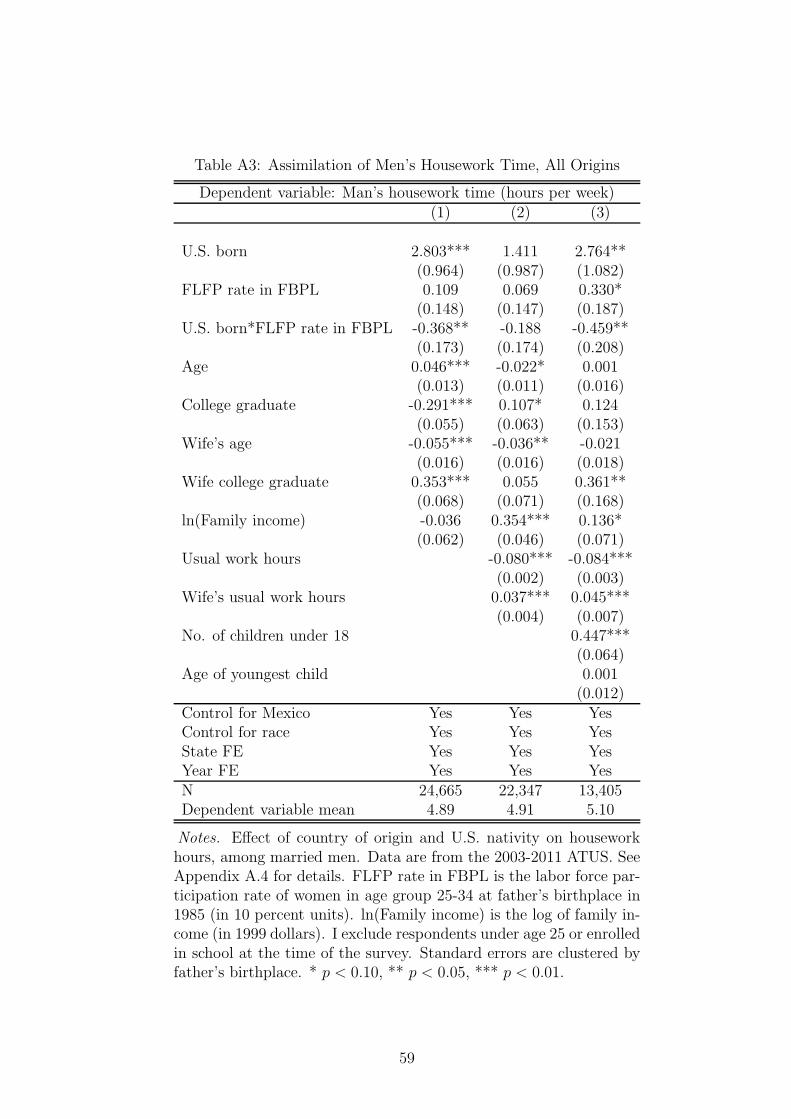
Table A3: Assimilation of Men’s Housework Time, All Origins
Dependent variable: Man’s housework time (hours per week)(1) (2) (3)
U.S. born 2.803*** 1.411 2.764**(0.964) (0.987) (1.082)
FLFP rate in FBPL 0.109 0.069 0.330*(0.148) (0.147) (0.187)
U.S. born*FLFP rate in FBPL -0.368** -0.188 -0.459**(0.173) (0.174) (0.208)
Age 0.046*** -0.022* 0.001(0.013) (0.011) (0.016)
College graduate -0.291*** 0.107* 0.124(0.055) (0.063) (0.153)
Wife’s age -0.055*** -0.036** -0.021(0.016) (0.016) (0.018)
Wife college graduate 0.353*** 0.055 0.361**(0.068) (0.071) (0.168)
ln(Family income) -0.036 0.354*** 0.136*(0.062) (0.046) (0.071)
Usual work hours -0.080*** -0.084***(0.002) (0.003)
Wife’s usual work hours 0.037*** 0.045***(0.004) (0.007)
No. of children under 18 0.447***(0.064)
Age of youngest child 0.001(0.012)
Control for Mexico Yes Yes YesControl for race Yes Yes YesState FE Yes Yes YesYear FE Yes Yes YesN 24,665 22,347 13,405Dependent variable mean 4.89 4.91 5.10
Notes. Effect of country of origin and U.S. nativity on houseworkhours, among married men. Data are from the 2003-2011 ATUS. SeeAppendix A.4 for details. FLFP rate in FBPL is the labor force par-ticipation rate of women in age group 25-34 at father’s birthplace in1985 (in 10 percent units). ln(Family income) is the log of family in-come (in 1999 dollars). I exclude respondents under age 25 or enrolledin school at the time of the survey. Standard errors are clustered byfather’s birthplace. * p < 0.10, ** p < 0.05, *** p < 0.01.
59
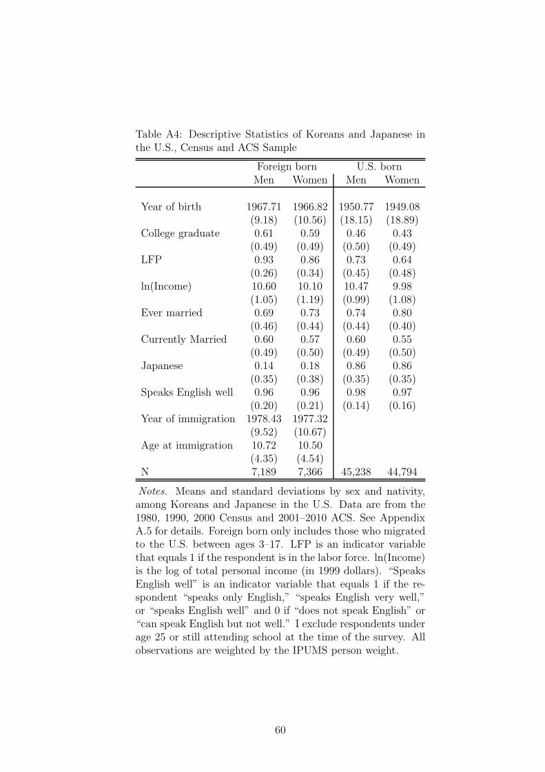
Table A4: Descriptive Statistics of Koreans and Japanese inthe U.S., Census and ACS Sample
Foreign born U.S. bornMen Women Men Women
Year of birth 1967.71 1966.82 1950.77 1949.08(9.18) (10.56) (18.15) (18.89)
College graduate 0.61 0.59 0.46 0.43(0.49) (0.49) (0.50) (0.49)
LFP 0.93 0.86 0.73 0.64(0.26) (0.34) (0.45) (0.48)
ln(Income) 10.60 10.10 10.47 9.98(1.05) (1.19) (0.99) (1.08)
Ever married 0.69 0.73 0.74 0.80(0.46) (0.44) (0.44) (0.40)
Currently Married 0.60 0.57 0.60 0.55(0.49) (0.50) (0.49) (0.50)
Japanese 0.14 0.18 0.86 0.86(0.35) (0.38) (0.35) (0.35)
Speaks English well 0.96 0.96 0.98 0.97(0.20) (0.21) (0.14) (0.16)
Year of immigration 1978.43 1977.32(9.52) (10.67)
Age at immigration 10.72 10.50(4.35) (4.54)
N 7,189 7,366 45,238 44,794
Notes. Means and standard deviations by sex and nativity,among Koreans and Japanese in the U.S. Data are from the1980, 1990, 2000 Census and 2001–2010 ACS. See AppendixA.5 for details. Foreign born only includes those who migratedto the U.S. between ages 3–17. LFP is an indicator variablethat equals 1 if the respondent is in the labor force. ln(Income)is the log of total personal income (in 1999 dollars). “SpeaksEnglish well” is an indicator variable that equals 1 if the re-spondent “speaks only English,” “speaks English very well,”or “speaks English well” and 0 if “does not speak English” or“can speak English but not well.” I exclude respondents underage 25 or still attending school at the time of the survey. Allobservations are weighted by the IPUMS person weight.
60
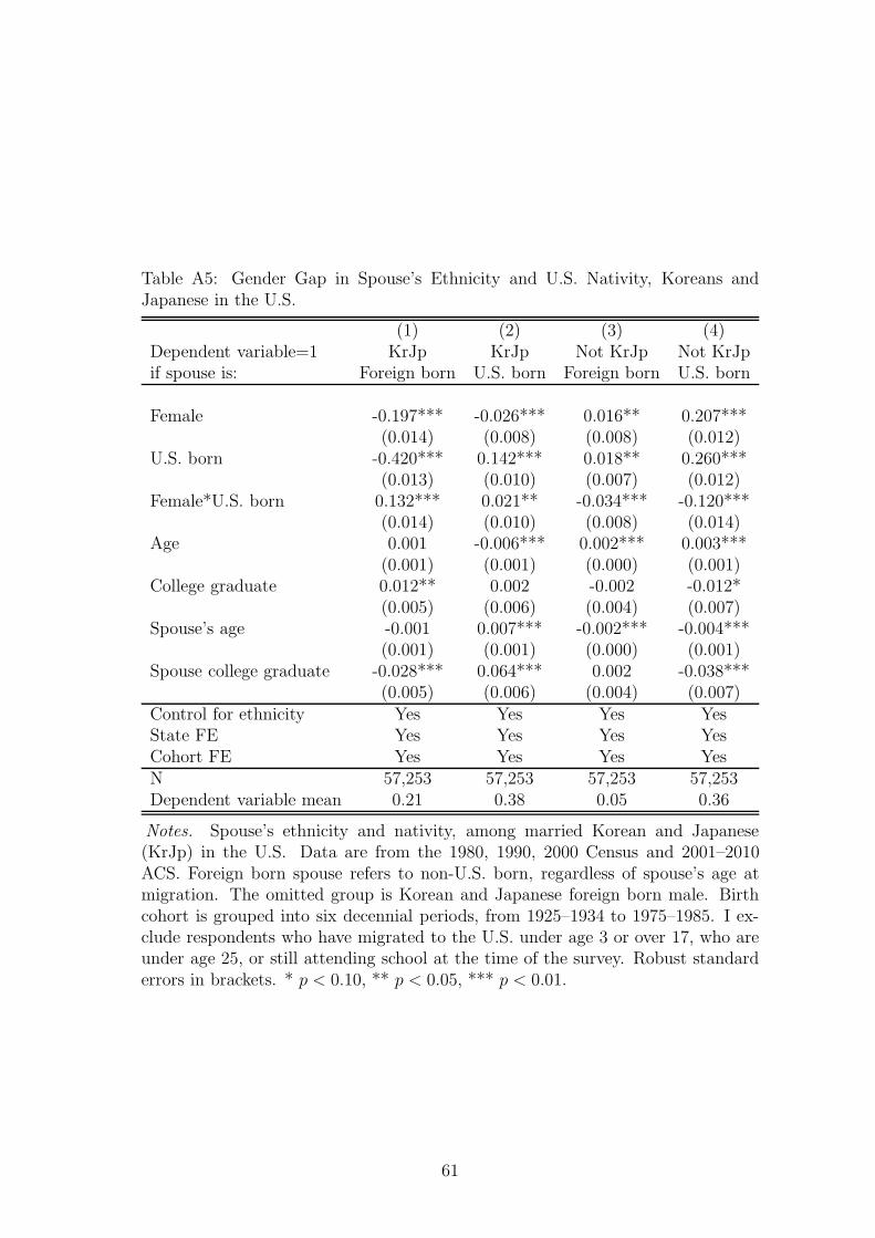
Table A5: Gender Gap in Spouse’s Ethnicity and U.S. Nativity, Koreans andJapanese in the U.S.
(1) (2) (3) (4)Dependent variable=1 KrJp KrJp Not KrJp Not KrJpif spouse is: Foreign born U.S. born Foreign born U.S. born
Female -0.197*** -0.026*** 0.016** 0.207***(0.014) (0.008) (0.008) (0.012)
U.S. born -0.420*** 0.142*** 0.018** 0.260***(0.013) (0.010) (0.007) (0.012)
Female*U.S. born 0.132*** 0.021** -0.034*** -0.120***(0.014) (0.010) (0.008) (0.014)
Age 0.001 -0.006*** 0.002*** 0.003***(0.001) (0.001) (0.000) (0.001)
College graduate 0.012** 0.002 -0.002 -0.012*(0.005) (0.006) (0.004) (0.007)
Spouse’s age -0.001 0.007*** -0.002*** -0.004***(0.001) (0.001) (0.000) (0.001)
Spouse college graduate -0.028*** 0.064*** 0.002 -0.038***(0.005) (0.006) (0.004) (0.007)
Control for ethnicity Yes Yes Yes YesState FE Yes Yes Yes YesCohort FE Yes Yes Yes YesN 57,253 57,253 57,253 57,253Dependent variable mean 0.21 0.38 0.05 0.36
Notes. Spouse’s ethnicity and nativity, among married Korean and Japanese(KrJp) in the U.S. Data are from the 1980, 1990, 2000 Census and 2001–2010ACS. Foreign born spouse refers to non-U.S. born, regardless of spouse’s age atmigration. The omitted group is Korean and Japanese foreign born male. Birthcohort is grouped into six decennial periods, from 1925–1934 to 1975–1985. I ex-clude respondents who have migrated to the U.S. under age 3 or over 17, who areunder age 25, or still attending school at the time of the survey. Robust standarderrors in brackets. * p < 0.10, ** p < 0.05, *** p < 0.01.
61
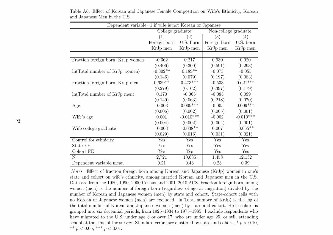
Table A6: Effect of Korean and Japanese Female Composition on Wife’s Ethnicity, Koreanand Japanese Men in the U.S.
Dependent variable=1 if wife is not Korean or JapaneseCollege graduate Non-college graduate(1) (2) (3) (4)
Foreign born U.S. born Foreign born U.S. bornKrJp men KrJp men KrJp men KrJp men
Fraction foreign born, KrJp women -0.362 0.217 0.930 0.020(0.406) (0.300) (0.591) (0.293)
ln(Total number of KrJp women) -0.302** 0.189** -0.073 -0.055(0.146) (0.079) (0.197) (0.083)
Fraction foreign born, KrJp men 0.639** 0.473*** -0.533 0.621***(0.279) (0.162) (0.397) (0.179)
ln(Total number of KrJp men) 0.170 -0.065 -0.085 0.099(0.149) (0.063) (0.218) (0.070)
Age -0.003 0.009*** -0.005 0.009***(0.006) (0.002) (0.005) (0.001)
Wife’s age 0.001 -0.010*** -0.002 -0.010***(0.004) (0.002) (0.004) (0.001)
Wife college graduate -0.003 -0.038** 0.007 -0.055**(0.029) (0.016) (0.031) (0.021)
Control for ethnicity Yes Yes Yes YesState FE Yes Yes Yes YesCohort FE Yes Yes Yes YesN 2,721 10,635 1,458 12,132Dependent variable mean 0.21 0.43 0.23 0.39
Notes. Effect of fraction foreign born among Korean and Japanese (KrJp) women in one’sstate and cohort on wife’s ethnicity, among married Korean and Japanese men in the U.S.Data are from the 1980, 1990, 2000 Census and 2001–2010 ACS. Fraction foreign born amongwomen (men) is the number of foreign born (regardless of age at migration) divided by thenumber of Korean and Japanese women (men) by state and cohort. State-cohort cells withno Korean or Japanese women (men) are excluded. ln(Total number of KrJp) is the log ofthe total number of Korean and Japanese women (men) by state and cohort. Birth cohort isgrouped into six decennial periods, from 1925–1934 to 1975–1985. I exclude respondents whohave migrated to the U.S. under age 3 or over 17, who are under age 25, or still attendingschool at the time of the survey. Standard errors are clustered by state and cohort. * p < 0.10,** p < 0.05, *** p < 0.01.
62
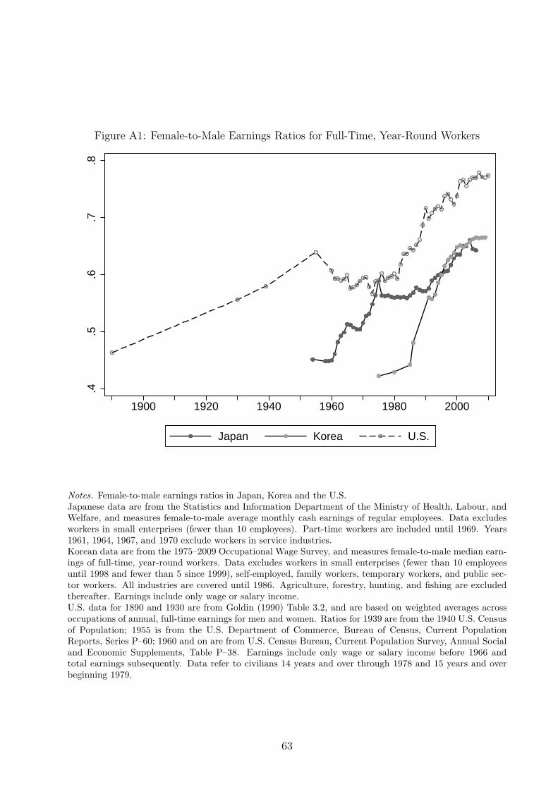
Figure A1: Female-to-Male Earnings Ratios for Full-Time, Year-Round Workers
.4.5
.6.7
.8
1900 1920 1940 1960 1980 2000
Japan Korea U.S.
Notes. Female-to-male earnings ratios in Japan, Korea and the U.S.Japanese data are from the Statistics and Information Department of the Ministry of Health, Labour, andWelfare, and measures female-to-male average monthly cash earnings of regular employees. Data excludesworkers in small enterprises (fewer than 10 employees). Part-time workers are included until 1969. Years1961, 1964, 1967, and 1970 exclude workers in service industries.Korean data are from the 1975–2009 Occupational Wage Survey, and measures female-to-male median earn-ings of full-time, year-round workers. Data excludes workers in small enterprises (fewer than 10 employeesuntil 1998 and fewer than 5 since 1999), self-employed, family workers, temporary workers, and public sec-tor workers. All industries are covered until 1986. Agriculture, forestry, hunting, and fishing are excludedthereafter. Earnings include only wage or salary income.U.S. data for 1890 and 1930 are from Goldin (1990) Table 3.2, and are based on weighted averages acrossoccupations of annual, full-time earnings for men and women. Ratios for 1939 are from the 1940 U.S. Censusof Population; 1955 is from the U.S. Department of Commerce, Bureau of Census, Current PopulationReports, Series P–60; 1960 and on are from U.S. Census Bureau, Current Population Survey, Annual Socialand Economic Supplements, Table P–38. Earnings include only wage or salary income before 1966 andtotal earnings subsequently. Data refer to civilians 14 years and over through 1978 and 15 years and overbeginning 1979.
63
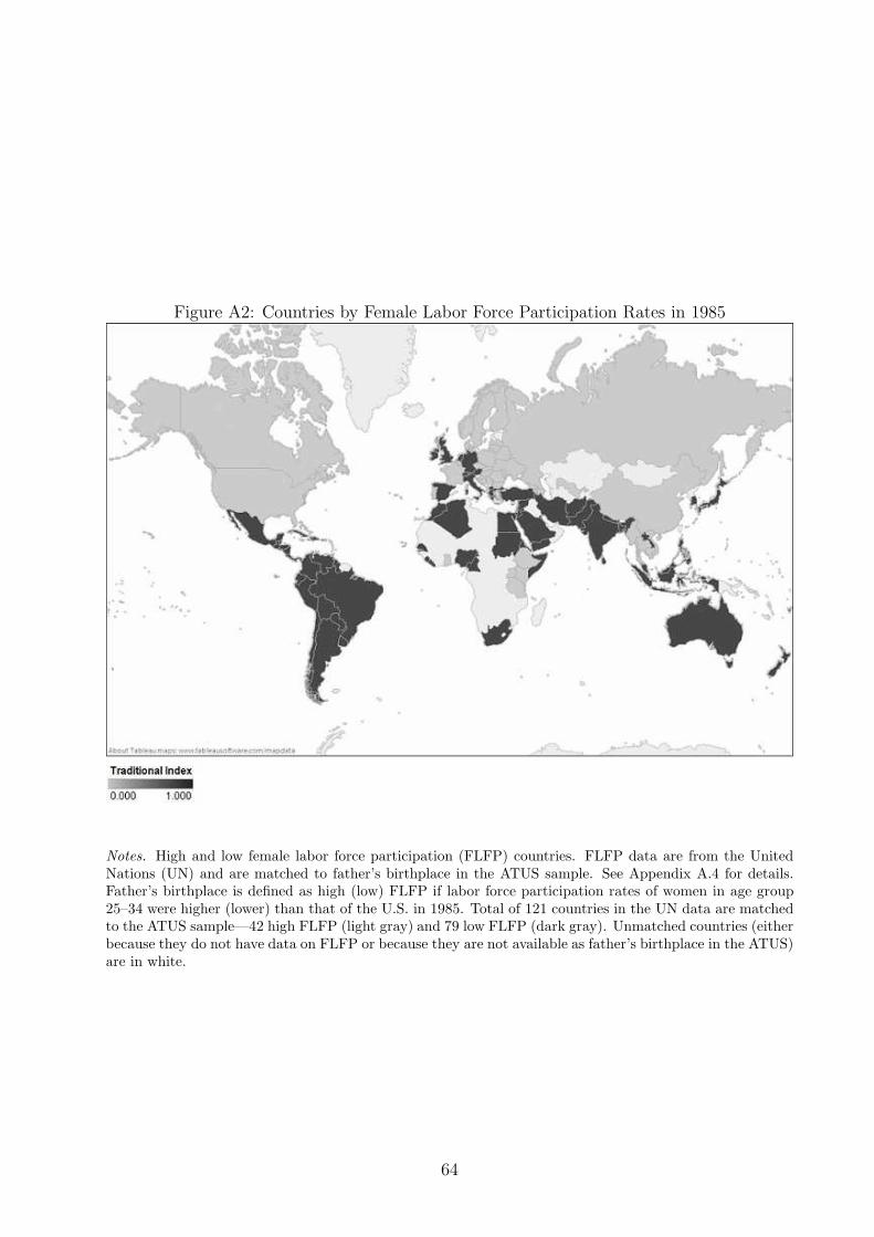
Figure A2: Countries by Female Labor Force Participation Rates in 1985
Notes. High and low female labor force participation (FLFP) countries. FLFP data are from the UnitedNations (UN) and are matched to father’s birthplace in the ATUS sample. See Appendix A.4 for details.Father’s birthplace is defined as high (low) FLFP if labor force participation rates of women in age group25–34 were higher (lower) than that of the U.S. in 1985. Total of 121 countries in the UN data are matchedto the ATUS sample—42 high FLFP (light gray) and 79 low FLFP (dark gray). Unmatched countries (eitherbecause they do not have data on FLFP or because they are not available as father’s birthplace in the ATUS)are in white.
64
Related Documents


![Annie May Housewife - Amazon S3€¦ · KERSEY Elgin Retired Mrs Housewife KERSEY John T. Retired Mailman KERSHAW [Jackson] Jackie Secretary / Typist KELLY Angus Electrician KELLY](https://static.cupdf.com/doc/110x72/5f2e8e5d92b86b002f473be0/annie-may-housewife-amazon-s3-kersey-elgin-retired-mrs-housewife-kersey-john-t.jpg)