Household Production and Life- Cycle and Labor Supply.

Household Production and Life-Cycle and Labor Supply

Household Production

• As in the study of labor demand, we can alter the variables to explore the impacts of utility maximization and the accompanying income and substitution effects of labor supply.

• In the previous analysis, we ignored household production. Household production of goods and services is an alternative to participation in the labor force and purchased goods and services that flow from that participation.

Assumptions

• Two alternatives: Purchased goods and services that come from working for pay and home produced goods and services that come from hours spent at home.

• Hours spent at home are directly related to home produced goods.

• Assume that leisure is zero• Single decision-maker• Household does not save or borrow

Graphical Model• Value of purchased goods and services on Y axis and hours spend

at home on the X axis (proxies value of home production)• Hours spent at home = 16 hours - Hours spent working for pay• Hh = 16 – H• Value of purchased goods and services is equal to Y = W x H• Constraint is similar to previous model with a slope of -W• Indifference curves or utility isoquants assume that home produced

goods (GS) and services and substitutes for purchased goods and services (Hh)

• The utility isoquants are convex reflecting that:– High GS and low Hh : ΔGS/ΔHh is high or isoquant is steeper– Low GS and high Hh : ΔGS/ΔHh is low or isoquant is flatter

• Ray from the origin reflects ration of GS to Hh

• If GS/Hh is high, ΔGS/ΔHh is also relatively high. When you an extra hour of Hh one has to give up a lot of purchased goods and services to remain equally well off. Why? At low levels of Hh time spend at home is more highly valued relative to GS.

• If GS/Hh is low, ΔGS/ΔHh is also relatively low. When you an extra hour of Hh one has to give up only a few purchased goods and services to remain equally well off. Why? At high levels of Hh time spend at home is less highly valued relative to GS.

• Work preferrer has a flatter isoquant.• Home preferrer has a steeper isoquant.

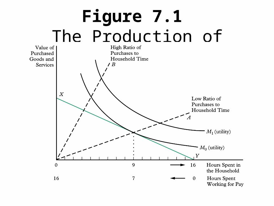
Figure 7.1 The Production of Child Care

Changes in Wages

• Changes in wages changes the “income/wage” constraint and produces income and substitution effects.

• The choice between time spent in the household and the time spent at work depends upon income and substitution effects

• The observed increases in participation rate of women and the convergence of participation rates with men indicates that the substitution effect has outweighed the income effect but the relatively strength of the substitution effect has been diminishing as participation rates approach those of men.

Tripartite Choice• The analysis can be expanded by including the labor-leisure

choice. Households must decide between time at work, time in household production and time spent in leisure.

• Two income and substitution effects as wages change. For example, as wages rise,– Substitute time in household for time at work

• Initially, time at household can more easily be given up through labor-saving devices and childcare. However, as participation rates and hours worked of breadwinners rises, this becomes more difficult.

– Substitute leisure for time at work• Leisure activities usually require time so it is more difficult to substitute for

them

• This may explain the initial rapid increase in participation and hours worked and why the trend is diminishing.

Figure 7.2 Large versus Small Substitution

Effects Attendant to a Wage Increase

Joint Labor Supply Decisions

• Dropping the assumption of one decision-maker, economists have looked at models of joint labor supply:– Retain single decision-maker either home

dictator or identical preferences.– Bargaining process with resources determining

bargaining power.– Act independently, but consider the impacts of

their actions on the other party.

Figure 7.3 Home versus Market

Productivities

• Specialization: household utility maximization with different productivities.– Productivity in work place– Productivity at home (household productivity and satisfaction from child-rearing).– Some studies demonstrate the division of housework depends on the relative wage

• Many households maximize utility with both individuals working. See graph.

• Cross effects: Spouse’s decision to work more for pay affects the other spouse household productivity in production or consumption.– If spouses are substitutes in household production, if one spouse works more the

other may become more productive and increase the amount of time they stay at home. If they are complements, the other may work more.

– If spouses are complements in consumption, the other may work more. Substitutes in consumption reflect a problematic marriage so…

Household Productivity in Recessions

• Recession causes spouse to become unemployed:– The unemployed workers productivity at work drops and

the opportunity cost of working at home goes down. – The relative productivity of the worker’s spouse rises if

their potential wages do not change.– Substitute unemployed worker for spouse’s participation

in household production and the spouse goes to work.– As family income falls, less goods and services and less

leisure time are demanded.– This creates an “additional worker” effect.

• On the other hand, the expected wage of either spouse may have also fallen.

• Decreases in expected wages create a substitution effect towards less work and more leisure.

• This would tend to create a “discouraged worker” effect.

• Discouraged and part-time workers are part of “hidden” unemployment.

Life Cycle Aspects

• Dynamic preferences or labor productivity at home and changing labor participation patterns– Presence of young children can make an

indifference curve steeper and the absence of younger children make the indifference curve flatter.

– Presence of a disabled child, parent or spouse could also have similar effects.

Figure 7.4 Household

Productivity Can Change over the Life

Cycle

Figure 7.5 Life-Cycle Allocation of Time

• An individual or household unit strives to maximize its present discounted wealth, which includes both wages from work and the value of household production.

• Individuals will work the most in those years with the greatest difference between wages and productivity at home.

• Scheduling vacations with market wage and household productivity. (e.g. Chile in the summer)

• Once time is considered, life-time wealth and the expected wage path that generates the life-time wealth may become more important that current wages.– If wage increase is expected, meaning that it follows the expected wage path, it will

not change life-time wealth. Therefore, the change in expected wages will create only a substitution effect.

– If the wage increases is unexpected, meaning the expected wage path changes, it will change life-time income. This will generate both a substitution and an income effect.

Choice of Retirement Age

• The budget constraint: See spreadsheet.• Increases in social security benefits:

– Increase in the fixed amount of benefits in each retirement year

• No substitution effect and retirement would be accelerated.

– Decrease in penalties from delaying retirement retirement (higher net wages in later years)

• Create a substitution effect towards later retirement• Create an income effect to retire earlier• If the decision is between participation and non-participation,

the substitution effect is likely to dominate

Figure 7.6 Choice of Optimum Retirement Age for Hypotheti

cal Worker

(based on data in

Table 7.2)

Child Care

• Forty percent of US families pay for child care and cost about 7% of family income.

• Child care costs involve fixed costs so that the average cost for limited child care is more than for full child care.

• Reducing the fixed costs of care:– Assume a level of non-earned income– Cover the fixed cost of child care

• Person not working chooses to work • Person not working chooses to continue not to work• Person working will choose to work less

Figure 7.7 Labor Supply and Fixed Child-Care

Costs: A Parent Initially out of the Labor

Force

Figure 7.8 Labor Supply and Fixed Child-Care

Costs: A Parent Initially Working for Pay

• Reducing the costs of hourly care– The hourly child care costs are like a tax rate on wages– A subsidy that reduces hourly wages would act like a wage

increase• Substitution effect towards more work

– A strong substitution effect for those out of the labor force and likely to increase participation rates

• Income effect towards more work

• Subsidy that reduce both the fixed and hourly costs increase participation rates but have an ambiguous effect on hours worked among those in the labor force.

Child Support Assurance• Many children in poverty live in single-parent households.

One persistent problem is that the absent parent often does not contribute to the children’s financial support.

• Programs that guarantee government support when private support is not forthcoming are likely to affect the labor supply decision of the single-parent.

• The budget constraint:– Work– Work and welfare guaranteeing a given income– Work and welfare and guaranteed child support regardless of

income.

Figure 7.10 A Single

Parent Who Joins the

Labor Force after Child

Support Assurance Program Adopted

Figure 7.9 Budget

Constraints Facing a

Single Parent before and after Child

Support Assurance Program Adopted