Household Bargaining and Portfolio Choice * Urvi Neelakantan † , Angela Lyons, and Carl Nelson University of Illinois at Urbana-Champaign December 2008 Preliminary Draft Abstract Differences in risk preferences may lead to spouses having different preferences over the allocation of their household portfolio. This pa- per examines how their problem is resolved using a simple collective model of household portfolio choice. The model predicts that the risk aversion of the spouse with more bargaining power determines house- hold portfolio allocation. The model also predicts that the share of risky assets in the household portfolio increases with wealth. Empir- ical support for the results is found using data from the Health and Retirement Study (HRS). 1 Introduction Households make financial decisions along two main dimensions. They decide how to allocate their income between consumption and savings and how to allocate their savings between risky and risk-free assets. The literature often * We thank Anna Paulson for numerous helpful comments. All remaining errors are ours. † Corresponding Author. Department of Agricultural and Consumer Economics, Uni- versity of Illinois at Urbana-Champaign, 1301 W. Gregory Dr., 421 Mumford Hall, Urbana, IL 61801, Ph: 217-333-0479, E-mail: [email protected]. 1

Welcome message from author
This document is posted to help you gain knowledge. Please leave a comment to let me know what you think about it! Share it to your friends and learn new things together.
Transcript
Household Bargaining and Portfolio Choice∗
Urvi Neelakantan†, Angela Lyons, and Carl Nelson
University of Illinois at Urbana-Champaign
December 2008Preliminary Draft
Abstract
Differences in risk preferences may lead to spouses having differentpreferences over the allocation of their household portfolio. This pa-per examines how their problem is resolved using a simple collectivemodel of household portfolio choice. The model predicts that the riskaversion of the spouse with more bargaining power determines house-hold portfolio allocation. The model also predicts that the share ofrisky assets in the household portfolio increases with wealth. Empir-ical support for the results is found using data from the Health andRetirement Study (HRS).
1 Introduction
Households make financial decisions along two main dimensions. They decide
how to allocate their income between consumption and savings and how to
allocate their savings between risky and risk-free assets. The literature often
∗We thank Anna Paulson for numerous helpful comments. All remaining errors areours.
†Corresponding Author. Department of Agricultural and Consumer Economics, Uni-versity of Illinois at Urbana-Champaign, 1301 W. Gregory Dr., 421 Mumford Hall, Urbana,IL 61801, Ph: 217-333-0479, E-mail: [email protected].
1
models such decisions using a unitary framework, which treats the house-
hold as a single decision-making unit with one utility function and pooled
income. A limitation of this approach is that it cannot analyze the influence
of individual household members with different preferences on household fi-
nancial decisions. Papers that do allow household members to have separate
preferences have shown that this is an important consideration. For exam-
ple, Browning (2000) and Mazzocco (2004) find that the allocation of re-
sources within the household affects the consumption-savings decision when
spouses differ in their preferences. Empirical estimates show that a majority
of spouses do indeed differ in risk preferences (Barsky, Juster, Kimball, and
Shapiro, 1997; Kimball, Sahm, and Shapiro, 2008).
This paper focuses on the household’s decision to allocate its savings
between risky and risk-free assets (hereafter household portfolio choice or
allocation). As economic changes place greater responsibility on households
to manage their own portfolios, it has become increasingly important for
economists and policy makers to understand how households make this de-
cision.
The literature on household portfolio choice is vast. The benchmark
model, which treats the household as a single agent with constant relative risk
aversion, predicts that household portfolio choice is independent of wealth.
Yet, empirical evidence suggests that the share of the household portfolio
allocated to risky assets increases with wealth (Bertaut and Starr-McCluer,
2002) and that the risk preferences of individual members are a significant
2

determinant of household portfolio choice (Charles and Hurst, 2003; Barsky,
Juster, Kimball, and Shapiro, 1997; Kimball, Sahm, and Shapiro, 2008). This
paper provides a model of household portfolio choice that is consistent with
this evidence. The model illustrates how intra-household differences in risk
aversion and bargaining power interact with wealth to determine household
portfolio choice. The model predicts that the risk aversion of the spouse
with more bargaining power determines household portfolio allocation. The
model also predicts that the share of risky assets in the household portfolio
increases with household wealth.
The predictions of the model are tested using data from the Health and
Retirement Study (HRS). The HRS is a longitudinal study that has surveyed
older Americans every other year since 1992.1 The HRS includes detailed
information on household portfolios and a series of questions that can be
used to infer respondents’ risk aversion.
Preliminary empirical evidence suggests that the predictions of the model
are consistent with the data.
2 Literature Review
The basic premise of this study is that marriage adds an additional layer of
complexity to household portfolio choice. In particular, household portfolio
decisions may be the outcome of bargaining because spouses may differ in
1The HRS is sponsored by the National Institute of Aging (grant number NIAU01AG009740) and is conducted by the University of Michigan.
3
risk aversion. Previous research supports the assumption that spouses differ
in risk aversion. For example, recent theoretical research finds that matching
among couples is negatively assortative on risk aversion (Legros and Newman,
2007; Chiappori and Reny, 2006). Empirical evidence supports the assump-
tion as well. Respondents to the HRS were asked a series of questions about
choosing between two jobs: one that paid their current income with certainty
and the other that had a 50-50 chance of doubling their income or reducing it
by a certain fraction. Based on their answers, respondents could be grouped
into four risk tolerance categories in the 1992 HRS. Mazzocco (2004) finds
that around 50% of respondents fall into a different risk tolerance category
from their spouses.
Most previous research on bargaining power and household financial deci-
sions has focused on the consumption-savings choice (Browning, 2000; Lund-
berg, Startz, and Stillman, 2003). The problem arises because wives, who are
on average younger and expected to live longer than their husbands, prefer
to save more than their husbands. Browning (2000) uses a noncooperative
bargaining model to show that the share of savings in the household portfolio
depends on the distribution of income between spouses. Lundberg, Startz,
and Stillman (2003) provide empirical support for this argument, showing
that household consumption falls after the husband retires (and presumably
loses bargaining power).
Two studies that utilize the HRS to study bargaining power are Elder
and Rudolph (2003) and Friedberg and Webb (2006). Elder and Rudolph
4

(2003) focus on the sources of bargaining power and find that decisions are
more likely to be made by the household member with more financial knowl-
edge, more education, and a higher wage, irrespective of gender. They do not
explore how the distribution of bargaining power affects financial outcomes.
Friedberg and Webb (2006), in addition to examining the sources of bargain-
ing power, investigate the consequences of bargaining power on household
portfolio choice. They find that households tend to invest more heavily in
stocks as the husband’s bargaining power increases.
Finally, largely absent in the literature is a link between household bar-
gaining theory and empirical models of household portfolio choice. This
study attempts to fill that gap.
3 Theoretical Framework
The theoretical framework is constructed under the assumption that house-
hold members cooperate and make efficient decisions. The economy consists
of households with two agents, a and b, who live for two periods. In the first
period, each member of the household is endowed with wealth wi0, i = a, b.
The household can save using a risk-free asset, m, that earns a certain re-
turn, rm, and a risky asset, s, that earns a stochastic return, r̃s(θ), where
θ denotes the state of nature. Agents derive utility from consuming out of
wealth a public good in periods 0 and 1, c0 and c̃1(θ). The utility function of
each agent, ui, is increasing, concave, and twice continuously differentiable.
5

Since the solution to the household problem is efficient, it can then be
obtained as the solution to the following Pareto problem. Given w0 = wa0+wb
0,
r̃s, and rm, the household chooses consumption, c0 and c̃1, savings in the risk-
free asset, m0, and savings in the risky asset, s0, to solve
maxc0,c̃1,m0,s0
λ [ua(c0) + βaEua(c̃1)] + (1 − λ)[
ub(c0) + βbEub(c̃1)]
subject to
c0 + m0 + s0 ≤ w0
c̃1 ≤ (1 + r̃s1)s0 + (1 + rm)m0 ∀θ.
Here λ denotes the Pareto weight or relative bargaining power of spouse a
and βi the discount factor for each spouse.
Let x0 = m0 + s0 denote total household savings and let ρ = s0
x0
be the
share of household savings invested in the risky asset. We can rewrite the
above problem as
maxx0,ρ
λ [ua(w0 − x0) + βaEua ((1 + r̃s1)ρx0 + (1 + rm)(1 − ρ)x0)]
+ (1 − λ)[
ub(w0 − x0) + βbEub ((1 + r̃s1)ρx0 + (1 + rm)(1 − ρ)x0)
]
.
Now assume that each agent has a constant relative risk aversion (CRRA)
6
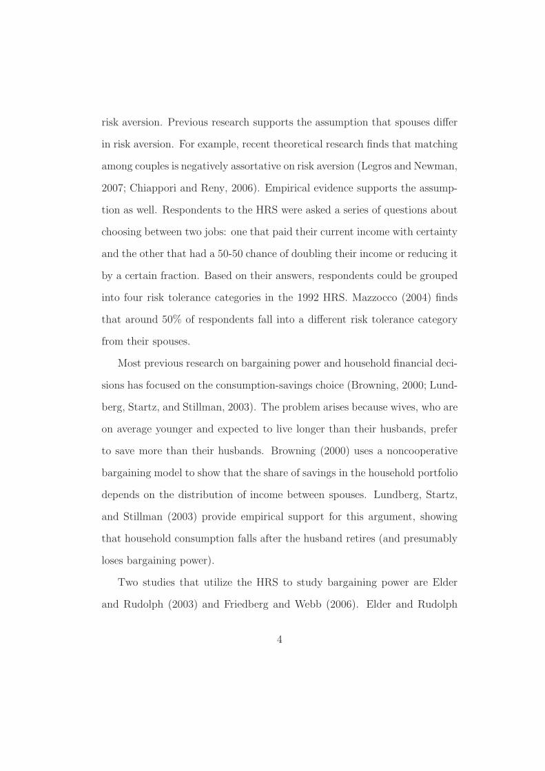
utility function of the form2
ua(ct) =c1−γa
t − 1
1 − γaand ub(ct) =
c1−γb
t − 1
δ(1 − γb).
The optimal choice of savings and portfolio allocation, x⋆0 and ρ⋆, are the
solution to the following first order conditions:
λδβax⋆γb
−γa
0
βb(1 − λ)
{
−(w0 − x⋆
0)−γa
βax⋆−γa
0
+ E [(1 + r̃s1)ρ
⋆ + (1 + rm)(1 − ρ⋆)]1−γa
}
+
{
−(w0 − x⋆
0)−γb
βbx⋆−γb
0
+ E [(1 + r̃s1)ρ
⋆ + (1 + rm)(1 − ρ⋆)]1−γb
}
= 0 (1)
λδβax⋆γb
−γa
0
βb(1 − λ)E
{
[(1 + r̃s1)ρ
⋆ + (1 + rm)(1 − ρ⋆)]−γa
(r̃s − rm)}
+
E{
[(1 + r̃s1)ρ
⋆ + (1 + rm)(1 − ρ⋆)]−γb
(r̃s − rm)}
= 0. (2)
Note that if δ = 1 and individual members of the household have equal Pareto
weights, identical discount factors, β, and identical coefficients of relative risk
aversion, γ, then (2) reduces to the following:
E{
[(1 + r̃s1)ρ
⋆ + (1 + rm)(1 − ρ⋆)]−γ (r̃s − rm)}
= 0. (3)
2The parameter δ is required for accurate numerical simulation. Assume that γa < γb.There is a threshold level of household wealth, w̄, above which “household risk aversion”is closer to γa and below which it is closer to γb. The threshold can be set at an arbitraryvalue by changing the value of δ. The details are described later.
7

Equation 3 represents the classic Merton-Samuelson result that the house-
hold’s choice of ρ is independent of its wealth.3
Before turning to the numerical solution to the problem, insights about
household portfolio choice can be gained by deriving the expression for house-
hold risk aversion. Define the instantaneous utility function of the represen-
tative agent as:4
V (w) = maxc
λc1−γa
1 − γa+ (1 − λ)
c1−γb
δ(1 − γb)
subject to
c ≤ w.
Household relative risk aversion is thus given by
γhh ≡ −wV ′′(w)
V ′(w)=
λδγaw−γa
+ (1 − λ)γbw−γb
λδw−γa + (1 − λ)w−γb
The main result can now be proved with the help of two lemmas.
Lemma 1. a) As the relative bargaining power of the more(less) risk-averse
spouse increases, household risk aversion increases(decreases).
b) An increase in wealth, w, reduces household relative risk aversion.
Lemma 2. As household risk aversion increases (decreases), the solution to
the household’s problem approaches the solution preferred by the more(less)
3Merton (1969); Samuelson (1969); also see Jagannathan and Kocherlakota (1996)4This is common in the literature on heterogeneous risk preferences. See, for example,
Dumas (1989) and Mazzocco (2003)
8

risk-averse spouse.
Proposition 1. As the relative bargaining power of a spouse increases, the
solution to the household’s problem approaches the solution most preferred by
that spouse.
Proof. In the Appendix
Finally, observe that if spouse i can dictate his or her preferences (i.e., if
λ = 0 or 1), the optimal share of the risky asset in the household portfolio is
the solution to
E{
[(1 + r̃s1)ρ
⋆ + (1 + rm)(1 − ρ⋆)]−γi
(r̃s − rm)}
= 0. (4)
where i = a if λ = 1 and i = b if λ = 0. We know from the numerical solution
to Equation (4) that as an individual’s risk aversion decreases, they prefer to
hold a greater share of their portfolio in the risky asset. Proposition 1 thus
implies that a greater share of the household’s portfolio will be invested in the
risky asset as the bargaining power of the less risk averse spouse increases.
This is shown in the numerical simulations below along with other properties
of the model.
3.1 Numerical Simulation
Since the theoretical model cannot be solved analytically, we describe the
properties of the model using numerical simulations. In particular, we are
9

interested in how risk aversion, bargaining power, and wealth interact to
determine optimal portfolio allocation, ρ⋆. To describe these relationships,
we numerically solve Equations (1) and (2) to calculate ρ⋆ for various values
of risk aversion, bargaining power, and wealth.
We assume throughout that the return on bonds, rm, is 1 percent and the
return on risky assets, rs1, is either 27.03 percent, 13 percent, or −15.25 per-
cent with equal probability.5 Numerically realistic simulations also require
choosing an appropriate value for δ. As mentioned earlier, given a threshold
level of household wealth, w̄, δ can be chosen such that household risk tol-
erance lies exactly between γa and γb at that level of wealth. The value of
δ for which this holds is δ = 1−λλ
w̄γa−γb
.6 To focus on gender differences in
risk preferences, we abstract from gender differences in time preferences for
the moment and assume that βa = βb = 0.95. Finally, we let γa = 4.8 and
γb = 8.2.7
3.1.1 Bargaining Power
To demonstrate the effect of bargaining power, we hold wealth constant and
show how the portfolio allocation changes with relative bargaining power.
5This yields a mean return of 8.26 percent with a standard deviation of 17.58 percent,which corresponds to the S&P 500 for 1871-2004. The return data is taken from http:
//www.econ.yale.edu/~shiller/data.htm.6This is obtained by solving γhh = γa
+γb
2. Alternately, δ can be chosen so that the
share of the household portfolio allocated to the risky asset lies exactly halfway betweenthe most preferred allocations of spouse a and b.
7These are the values estimated for risk category I and III in the HRS; see Barsky,Juster, Kimball, and Shapiro (1997).
10

Let w0 = $141, 200, which represents the mean financial assets of married
couples in the 2000 HRS.8 Let λ, which is spouse a’s relative bargaining power
within the household, vary from 0 to 1. Figure 1 shows the result. First,
note that if the relative bargaining power of spouse a equalled 1, then the
optimal portfolio allocation to the risky asset would be 48.4 percent. On the
other hand, if the relative bargaining power of spouse b was 1, the optimal
allocation would be 28.2 percent. The allocation lies somewhere between
these two values depending on the distribution of bargaining power within
the household.
Figure 1: Effect of relative bargaining power on portfolio allocation
30%
40%
50%
60%
Sh
are
of
Ris
ky
Ass
et
in H
ou
seh
old
Po
rtfo
lio
0%
10%
20%
0 0.2 0.4 0.6 0.8 1
Sh
are
of
Ris
ky
Ass
et
in H
ou
seh
old
Po
rtfo
lio
Bargaining Power of Spouse A
8Assets in Individual Retirement Accounts (IRAs) are excluded here and in the analysisbecause the HRS did not report what fraction of these were invested in risky assets.
11

3.1.2 Wealth
To demonstrate the effect of wealth, assume that the relative bargaining
power of both spouses is equal, that is, λ = 0.5. Let w0, wealth in period 1,
vary from $1,000 to $400,000. Figure 2 shows that the share of the household
portfolio allocated to the risky asset increases with wealth. When household
wealth is low, the allocation is closer to what the more risk averse spouse
prefers and when household wealth is high, the allocation is closer to what
the less risk averse spouse prefers.
Figure 2: Effect of Wealth on Portfolio Allocation
20%
25%
30%
35%
40%
45%
50%
Sh
are
of
Ris
ky
Ass
et
in H
ou
seh
old
Po
rtfo
lio
(ρ
)
0%
5%
10%
15%
20%
0 50000 100000 150000 200000 250000 300000 350000 400000
Sh
are
of
Ris
ky
Ass
et
in H
ou
seh
old
Po
rtfo
lio
(
Wealth (w0)
Finally, in Figure 3, both bargaining power and wealth are allowed to
vary. Each line represents a different level of wealth. The figure shows that
bargaining power matters most in the middle of the wealth distribution. For
low levels of wealth, the portfolio allocation remains close to the more risk
12

Figure 3: Interaction of Bargaining Power and Wealth
0.3
0.4
0.5
0.6
Sh
are
of
Ris
ky
Ass
et
in H
ou
seh
old
Po
rtfo
lio
(ρ
)
w0=50,000
w0=100,000
w0=150,000
w0=200,000
0
0.1
0.2
0 0.2 0.4 0.6 0.8 1
Sh
are
of
Ris
ky
Ass
et
in H
ou
seh
old
Po
rtfo
lio
(
Bargaining Power of Spouse A
w0=200,000
w0=250,000
w0=300,000
w0=350,000
averse spouse’s preferred choice while for high levels of wealth it remains
close to the less risk averse spouse’s preferred choice.
The theoretical model and simulations provide a number of empirically
testable predictions. The next section describes the data used to test these
predictions.
4 Data
The data comes from the 2000 wave of the HRS. The sample was restricted
to married (or partnered) couples with both spouses in the data set, which
yielded 6,279 married couples. Couples missing information about their years
of education were dropped, after which 6,239 couples remained. A further 602
13

observations for whom financial wealth was zero were dropped. Finally, those
for whom risk aversion data was missing were dropped, yielding a sample of
2,600 couples.
The risk tolerance data comes from Kimball, Sahm, and Shapiro (2008),
who constructed a cardinal measure of risk aversion using responses to a
series of questions in the HRS about choosing between two jobs: one that
paid the respondent their current income with certainty and the other that
had a 50-50 chance of doubling their income or reducing it by a certain
fraction. 9
Our variable of interest is the share of risky assets in household financial
wealth. We define household financial wealth as the sum of the net value of
assets in: 1) stocks, stock mutual funds, and investment trusts, 2) checking,
savings, and money market accounts, 3) certificates of deposit (CDs), savings
bonds, and Treasury bills, 4) bonds and bond funds and 5) other savings.
The first category, hereafter referred to as “stocks,” defines risky assets.
The characteristics of the sample are described in Table 1. Mean house-
hold financial wealth is $141,200. Over 42% of households hold some part of
this wealth in stocks. The average share of stocks is nearly 25%. The data
supports the premise of the paper that spouses differ in risk aversion; the
table shows that this is true of nearly 80% of couples in the sample. We use
years of education as our measure of bargaining power. The table shows that
9The data was downloaded from http://www-personal.umich.edu/~shapiro/data/
risk_preference/.
14
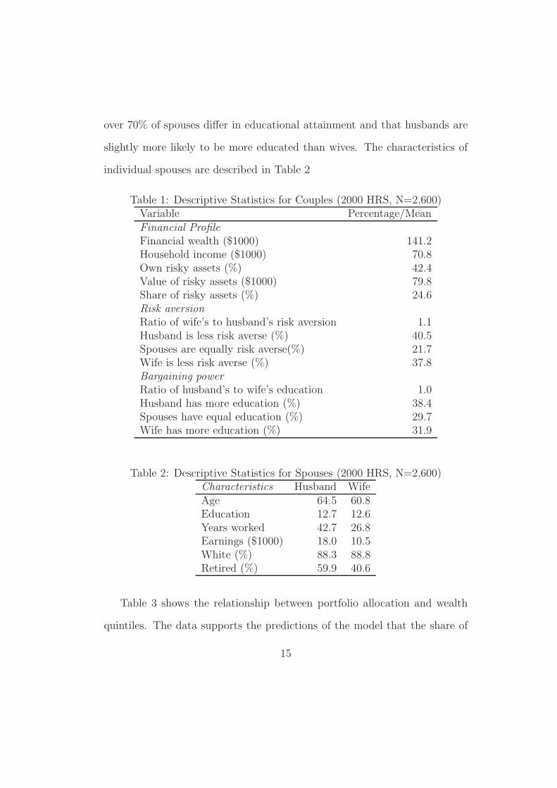
over 70% of spouses differ in educational attainment and that husbands are
slightly more likely to be more educated than wives. The characteristics of
individual spouses are described in Table 2
Table 1: Descriptive Statistics for Couples (2000 HRS, N=2,600)Variable Percentage/MeanFinancial ProfileFinancial wealth ($1000) 141.2Household income ($1000) 70.8Own risky assets (%) 42.4Value of risky assets ($1000) 79.8Share of risky assets (%) 24.6Risk aversionRatio of wife’s to husband’s risk aversion 1.1Husband is less risk averse (%) 40.5Spouses are equally risk averse(%) 21.7Wife is less risk averse (%) 37.8Bargaining powerRatio of husband’s to wife’s education 1.0Husband has more education (%) 38.4Spouses have equal education (%) 29.7Wife has more education (%) 31.9
Table 2: Descriptive Statistics for Spouses (2000 HRS, N=2,600)Characteristics Husband WifeAge 64.5 60.8Education 12.7 12.6Years worked 42.7 26.8Earnings ($1000) 18.0 10.5White (%) 88.3 88.8Retired (%) 59.9 40.6
Table 3 shows the relationship between portfolio allocation and wealth
quintiles. The data supports the predictions of the model that the share of
15

risky assets in the household portfolio increases with wealth.
Table 3: Shares of Risky Assets by Financial Wealth Quintiles (2000 HRS,N=2,600)Financial Wealth Quintile Share of Risky Asset (%)
1 1.92 7.73 23.14 35.65 55.8
5 Empirical Evidence
To test the predictions of the theoretical model, we define a variable
zi =λ
1 − λ
γa
γb
that is the product of relative bargaining power and relative risk aversion.
The variable z increases with the relative bargaining power of spouse a and
with his or her risk aversion. We hypothesize, controlling for wealth and
levels of risk aversion in the household, that ρi as a function of zi will have an
inverted-U shape. The argument goes as follows. When zi is small, it means
that spouse b is more risk averse and has more bargaining power relative to
spouse a. Thus the share of risky assets in the household portfolio, ρi, will
be small. When zi is large, it means that it means that spouse a is more risk
averse and has more bargaining power relative to spouse b. Again, ρi will be
16
small. The value of zi will fall between these two extremes when spouse a
has relatively more bargaining power and is less risk averse (λ large and γa
small) or when spouse b has relatively more bargaining power and is less risk
averse (1 − λ large and γb small). In either case, the share of risky assets in
the household portfolio will be large.
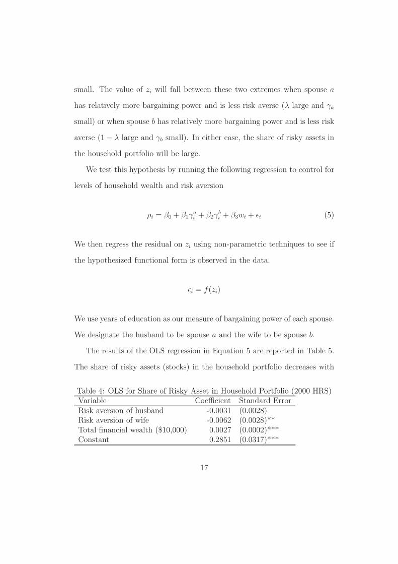
We test this hypothesis by running the following regression to control for
levels of household wealth and risk aversion
ρi = β0 + β1γai + β2γ
bi + β3wi + ǫi (5)
We then regress the residual on zi using non-parametric techniques to see if
the hypothesized functional form is observed in the data.
ǫi = f(zi)
We use years of education as our measure of bargaining power of each spouse.
We designate the husband to be spouse a and the wife to be spouse b.
The results of the OLS regression in Equation 5 are reported in Table 5.
The share of risky assets (stocks) in the household portfolio decreases with
Table 4: OLS for Share of Risky Asset in Household Portfolio (2000 HRS)Variable Coefficient Standard ErrorRisk aversion of husband -0.0031 (0.0028)Risk aversion of wife -0.0062 (0.0028)**Total financial wealth ($10,000) 0.0027 (0.0002)***Constant 0.2851 (0.0317)***
17
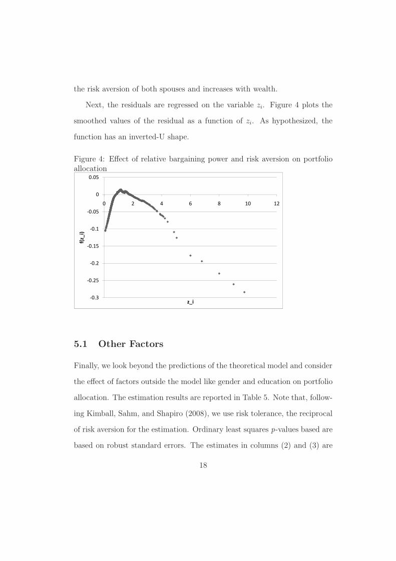
the risk aversion of both spouses and increases with wealth.
Next, the residuals are regressed on the variable zi. Figure 4 plots the
smoothed values of the residual as a function of zi. As hypothesized, the
function has an inverted-U shape.
Figure 4: Effect of relative bargaining power and risk aversion on portfolioallocation
-0.1
-0.05
0
0.05
0 2 4 6 8 10 12
f(z_i)
-0.3
-0.25
-0.2
-0.15
f(z_i)
z_i
5.1 Other Factors
Finally, we look beyond the predictions of the theoretical model and consider
the effect of factors outside the model like gender and education on portfolio
allocation. The estimation results are reported in Table 5. Note that, follow-
ing Kimball, Sahm, and Shapiro (2008), we use risk tolerance, the reciprocal
of risk aversion for the estimation. Ordinary least squares p-values based are
based on robust standard errors. The estimates in columns (2) and (3) are
18

exactly identified generalized method of moment (gmm) estimates proposed
by Kimball, Sahm, and Shapiro (2008). The p-values are based on bootstrap
standard errors because the risk tolerance variable is a generated regressor.
Table 5: OLS and GMM for Share of Risky Asset in Household Portfolio
(1) (2) (3)ols gmm gmm
Wife’s risk tolerance -0.219794 0.000148 -0.001207(0.026) (0.029) (0.000)
Wealth ($100,000) 049041 0.049543 0.061610(0.000) (0.000) (0.000)
Wealth squared -0.000530 -5.34e-08 -6.77e-08(0.000) (0.262) (0.234)
Ratio of husband’s to wife’s education -0.124311 -0.0946 0.114603(0.000) (0.000) (0.000)
Husband’s education 0.022560 0.019703(0.000) (0.000)
Education ratio x wife’s risk tolerance 0.353003 0.163986 0.242011(0.006) (0.024) (0.030)
N 2600 2600 2600
t-test p-values in parentheses
The gmm estimate in column (2) show that a $20,000 increase in financial
wealth causes a 1% increase in the share of risky assets. There is a strong
partial effect from the education of the husband. Moving from high school
education to a college education causes a 7.7% increase in the share of risky
assets. Overall, the empirical results indicate a first order effect of increasing
exposure to risky assets as the husband becomes more educated, and house-
19

hold wealth increases. There is a second order effect of further increase in
exposure to risky assets as the risk tolerance of the wife increases.
Comparing the estimates in column (2) and (3), we see that the coeffi-
cient on wealth, the square of wealth and the interaction term are consistent
if husband’s education is included or excluded. The coefficient on the edu-
cation ratio changes sign from negative to positive when husband’s eduction
is dropped. This suggests that investment in risky assets increases with the
education of the husband but the effect is weakened the larger the education
difference between the husband and the wife.
The positive coefficients on the interaction term is consistent across spec-
ifications and implies that as the husband’s relative eduction increases and
the wife’s risk tolerance increases more wealth is invested in risky assets.
6 Conclusion
This paper builds upon previous research by constructing a basic theoretical
framework to describe household portfolio choice for married couples. The
model predicts that household portfolio allocation is determined by the risk
preference of the spouse with more bargaining power. It also predicts that
the share of risky assets in the household portfolio increases with wealth.
Empirical evidence from the 2000 HRS supports these predictions.
Policymakers can use the findings to evaluate the impact of policies that
shift investment responsibilities to individuals, especially married couples.
20
As this study has shown, bargaining power and individual characteristics of
couples can significantly affect household portfolio decisions.
For the purposes of this paper, we assumed a cooperative bargaining
model in which the Pareto optimal solution for the couple is always attained.
It might be interesting to consider a non-cooperative framework. It is also
important to note that we only used data from the 2000 HRS. However,
the HRS is a longitudinal data set that is rich in financial and demographic
information for both husbands and wives. It would be of interest to look at
the impact that a change in bargaining power (say as a result of retirement)
has on household portfolio allocation. Finally, it is important to acknowledge
that the HRS collects data from a representative sample of older Americans.
Thus, it may not be possible to generalize our findings to the U.S. population
as a whole. While the HRS has detailed information on household decision-
making and household portfolio composition, it may be worth analyzing other
data that is representative of the U.S. population as a whole. Research is
currently underway to examine all these issues.
21

References
Barsky, R. B., F. T. Juster, M. S. Kimball, and M. D. Shapiro
(1997): “Preference Parameters and Behavioral Heterogeneity: An Exper-
imental Approach in the Health and Retirement Study,” The Quarterly
Journal of Economics, 112(2), 537–579.
Bertaut, C., and M. Starr-McCluer (2002): Household Portfo-
lioschap. 5, pp. 181–218. The MIT Press.
Browning, M. (2000): “The saving behavior of a two-person household,”
Scandinavian Journal of Economics, 102(2), 235–51.
Charles, K. K., and E. Hurst (2003): “The Correlation of Wealth across
Generations.,” Journal of Political Economy, 111(6), 1155 – 1182.
Chiappori, P.-A., and P. Reny (2006): “Matching to Share Risk,” Un-
published Manuscript.
Dumas, B. (1989): “Two-Person Dynamic Equilibrium in the Capital Mar-
ket,” The Review of Financial Studies, 2(2), 157–188.
Elder, H. W., and P. M. Rudolph (2003): “Who makes the financial de-
cisions in the households of older Americans?,” Financial Services Review,
12(4), 293–308.
Friedberg, L., and A. Webb (2006): “Determinants and consequences
22

of bargaining power in households,” Boston College Center for Retirement
Research Working Paper.
Jagannathan, R., and N. R. Kocherlakota (1996): “Why Should
Older People Invest Less in Stocks Than Younger People?,” Federal Re-
serve Bank of Minneapolis Quarterly Review, 20(3), 1123.
Kimball, M. S., C. R. Sahm, and M. D. Shapiro (2008): “Imputing
Risk Tolerance from Survey Responses,” Journal of the American Statis-
tical Association, forthcoming.
Legros, P., and A. F. Newman (2007): “Beauty Is a Beast, Frog Is
a Prince: Assortative Matching with Nontransferabilities,” Econometrica,
75(4), 1073–1102.
Lundberg, S., R. Startz, and S. Stillman (2003): “The retirement-
consumption puzzle: a marital bargaining approach,” Journal of Public
Economics, 87(5-6), 1199–1218.
Mazzocco, M. (2003): “Saving, Risk Sharing and Preferences for Risk,”
Working Paper, University of Wisconsin.
Mazzocco, M. (2004): “Saving, Risk Sharing, and Preferences for Risk,”
The American Economic Review, 94(4), 1169–1182.
Merton, R. C. (1969): “Lifetime Portfolio Selection under Uncertainty:
The Continuous-Time Case,” The Review of Economics and Statistics,
51(3), 247–257.
23

Samuelson, P. A. (1969): “Lifetime Portfolio Selection By Dynamic
Stochastic Programming,” The Review of Economics and Statistics, 51(3),
239–246.
24

A Proofs
A.1 Proof of Lemma 1
Proof. a) Assume without loss of generality that spouse a is less risk averse
than spouse b, i.e., γa < γb. Then
∂γhh
∂λ=
δw−γa−γb
(γa − γb)
(λδw−γa + (1 − λ)w−γb)2< 0
Thus an increase in λ, the relative bargaining power of the less risk averse
spouse, leads to a decrease in household risk aversion. A decrease in λ, i.e.,
an increase in (1 − λ), the relative bargaining power of the more risk averse
spouse, leads to an increase in household risk aversion.
b) The derivative of household risk aversion, γhh, with respect to wealth,
w, is given by
∂γhh
∂w=
−λ(1 − λ)δ(γa − γb)2w−(γa+γb+1)
(
λδw−γa + (1 − λ)w−γb)2 < 0
Thus household relative risk aversion decreases as wealth increases.
25

A.2 Proof of Lemma 2
Proof. After algebraic manipulation, we can rewrite the first order conditions
for the solution to the household’s problem as
ZX(a) + X(b) = 0
ZY (a) + Y (b) = 0.
where
Z =βa
βb
γhh − γb
γa − γhh
X(i) =
{
−(w0 − x⋆
0)−γi
βix⋆−γi
0
+ E [(1 + r̃s1)ρ
⋆ + (1 + rm)(1 − ρ⋆)]1−γi
}
, i = a, b
Y (i) = E{
[(1 + r̃s1)ρ
⋆ + (1 + rm)(1 − ρ⋆)]−γi
(r̃s − rm)}
, i = a, b
Spouse a’s most preferred solution is chosen when λ = 1. If λ = 1, the first
order conditions for the solution to the household’s problem are X(a) = 0
and Y (a) = 0. Spouse b’s most preferred solution is chosen when λ = 0. If
λ = 0, the first order conditions for the solution to the household’s problem
are X(b) = 0 and Y (b) = 0.
Suppose γa < γb. Then
∂Z
∂γhh=
γa − γb
(γa − γhh)2< 0
26
Thus as γhh increases, Z decreases, and the solution to the household problem
gets closer to the preferred solution of spouse b, the more risk averse spouse.
Now suppose γa > γb. Then
∂Z
∂γhh=
γb − γa
(γa − γhh)2> 0
Thus as γhh increases, Z decreases, and the solution to the household problem
gets closer to the preferred solution of spouse a, the more risk averse spouse.
A.3 Proof of Proposition 1
Proof. The proof follows directly from Lemma 1a and Lemma 2.
27
Related Documents