Hourly ozone prediction for a 24-h horizon using neural networks

lable at ScienceDirect

Environmental Modelling & Software 23 (2008) 1407–1421

Contents lists avai

Environmental Modelling & Software

journal homepage: www.elsevier .com/locate/envsoft

Hourly ozone prediction for a 24-h horizon using neural networks

Adriana Coman*, Anda Ionescu, Yves CandauCERTES, University of Paris XII, 61 avenue du General de Gaulle, F-94 010 Creteil Cedex, France

a r t i c l e i n f o

Article history:Received 5 March 2008Accepted 7 April 2008Available online 20 May 2008

Keywords:OzoneShort-term predictionNon-linear dynamicsNeural networksMultilayer perceptronGreater Paris

* Corresponding author. Tel.: þ33 1 45 17 18 29; faE-mail address: [email protected] (A. Coman

1 APHEIS: Air Pollution and Health: an Europeanapheis.net.

2 ERPURS: Monitoring of Short-Term Health Effects3 www.debatdeplacements.paris.fr/arrondissemen

rendu_Sante.pdf.

1364-8152/$ – see front matter � 2008 Elsevier Ltd.doi:10.1016/j.envsoft.2008.04.004

a b s t r a c t

This study is an attempt to verify the presence of non-linear dynamics in the ozone time series by testinga ‘‘dynamic’’ model, evaluated versus a ‘‘static’’ one, in the context of predicting hourly ozone concen-trations, one-day ahead. The ‘‘dynamic’’ model uses a recursive structure involving a cascade of 24multilayer perceptrons (MLP) arranged so that each MLP feeds the next one. The ‘‘static’’ model isa classical single MLP with 24 outputs. For both models, the inputs consist of ozone and of exogenousvariables: past 24-h values of meteorological parameters and of NO2; concerning the ozone inputs, the‘‘static’’ model uses only the 24 past measurements, while the ‘‘dynamic’’ one uses, also, the previouslyforecast ozone concentrations, as soon as they are predicted by the model. The outputs are, for bothconfigurations, ozone concentrations for a 24-h horizon. The performance of the two models wasevaluated for an urban and a rural site, in the greater Paris. Globally, the results indicate a rather goodapplicability of these models for a short-term prediction of ozone. We notice that the results of therecursive model were comparable with those obtained via the ‘‘static’’ one; thus, we can conclude thatthere is no evidence of non-linear dynamics in the ozone time series under study.

� 2008 Elsevier Ltd. All rights reserved.

1. Introduction

Predicting atmospheric pollutant concentrations in the greaterParis is a true challenge but, at the same time, a necessary actionallowing local authorities to take preventive measures, such astraffic limitations or public information.

The strong relationship between atmospheric pollution andhuman health was emphasised by many studies conducted for ourarea of interest or for others, e.g. the European project APHEIS,1

which emphasised the pollution effects on human health in 26cities from 12 European countries. Another good example is theregional project ERPURS,2 conducted in the greater Paris, with twodeclared goals: firstly to characterise the short-term relationshipbetween air pollution and the population health; secondly, to de-termine the feasibility of obtaining, from multiple sources and ona regular basis, the data needed to create a surveillance system ableto monitor this relationship (Medina et al., 1997). According toGrimfeld,3 ‘‘there are enough studies revealing the relationshipbetween air pollution and health. It is known nowadays that airpollution increases asthma [.]. One must not focus only on the

x: þ33 1 45 17 65 51.).Information System, www.

of Urban Air Pollution.t/telechargement/Compte_

All rights reserved.

pollution exceedances, it is important to be concerned also aboutthe medium-level pollution’’.

Modelling the ozone’s fluctuations and providing a good pre-diction are two of the most important tasks for the researchers.Two types of models can be used: deterministic or statistical (blackboxes). The use of partial differential equations to construct a de-terministic model to forecast the ozone concentrations in a limiteddomain is a rather complex process, which has to take into accounta large number of physical and chemical interactions betweenpredictor variables, and requires numerous accurate input data (e.g.emissions, meteorology and land cover). These are the main rea-sons why the deterministic models are very expensive to developand maintain.

Vautard et al. (2001) developed a hybrid statistical-deterministic chemistry-transport model for the ozone predictionin the Paris area, during Summer 1999. The model uses real-timeweather forecasts, performing ozone prediction up to three daysahead. The chemistry-transport model (CHIMERE) is forced at theboundaries by a statistical back trajectory-based model predictingthe background concentrations of a few species on a grid of 6�6 km cells. In the urban area, ozone levels are fairly well forecast,with correlation coefficients between forecast and observationsabout 0.7–0.8, and RMSE (cf. Section 3.4) in the range 15–20 mg m�3

at short-lead times, and 20–30 mg m�3 at long-lead times.In contrast with the deterministic models, the statistical ones

are easier to implement. There are many different approachestrying to establish a mathematical relationship between thepredictors (input variables) and predictands (output variables).

4 www.harmo.org/kit/default.asp.

A. Coman et al. / Environmental Modelling & Software 23 (2008) 1407–14211408

Generally, the statistical models are based on the detection of somepatterns, which are used later to forecast the desired pollutantconcentrations.

Among the statistical approaches, the artificial neural networks(ANN), and in particular multilayer perceptrons (MLP), were largelyapplied in the last decade for short-term prediction of gas andparticulate matter pollution. A complete review on applications ofmultilayer neural networks in the atmospheric sciences was writ-ten by Gardner and Dorling (1998). They show that the MLP can betrained to approximate any smooth measurable function and itdoesn’t make any assumptions concerning the data distribution.Maier and Dandy (2000) tried to establish the general context andto develop some guidelines for the application of these models intovarious research areas, like water resources. They analysed 43papers dealing with neural networks and remarked ‘‘the tendencyamong researchers to apply ANNs to problems for which othermethods have been unsuccessful’’.

In the last 10 years, many researchers in the environmentalfield have tried to improve the quality of ozone prediction fora horizon varying from 1 to 24 h. Viotti et al. (2002) applied ANNto forecast several pollutants: particulate matter, sulphur dioxide,nitrogen oxides, ozone, carbon monoxide and benzene (short- andmiddle–long-term prediction) using a general form of the logisticactivation function with three adjustable parameters and theback-propagation training algorithm. The selected inputs wererelated to the meteorological conditions and to the traffic levels.Abdul-Wahab and Al-Alawi (2002) focused on the identification ofthe factors that regulate the ozone levels during daylight andexamined the relative contribution of meteorology on the ozoneconcentration, a contribution found to vary within the range 33–41%. They also found an important contribution of the tempera-ture, NO, SO2, relative humidity and NO2, but lower effect thanexpected for the solar radiation.

Balaguer Ballester et al. (2002) present a comparison of severalpredictive models used to forecast 24 h in advance the hourlyozone concentration: (i) autoregressive-moving average with ex-ogenous inputs (ARMAX); (ii) multilayer perceptrons (MLP) and(iii) finite impulse response (FIR) neural network. They focused onthe ozone summer peaks recorded by three Spanish monitoringstations situated in urban or rural environment, from 1996 to 1999.The five performance criteria calculated yield reasonably goodresults and indicated that the MLP neural networks were moreeffective than the linear ARMAX models, which performed betterthan the dynamic FIR neural networks.

Within an exhaustive study, Schlink et al. (2003) tested 15 dif-ferent statistical techniques (the persistence model, multivariatelinear regression, autoregression, neural networks and generalisedadditive models) for ozone forecasting, applied to 10 data setsrepresenting different meteorological and emission conditionsthroughout Europe, and compared their performance with a de-terministic chemical trajectory model. According to their results,they reject the hypothesis of non-linear ozone dynamics and revealthe existence of static non-linearities between ozone, meteoro-logical parameters and concentrations of other pollutants. For thecomparison of different models using different data sets they rec-ommended the index of agreement (d2) and the success index SI (cf.Section 3.4). They obtained limited success indices for linear fore-casting techniques and a better prediction performance for bothneural networks and generalised additive models, which are able tohandle static non-linearities.

Kukkonen et al. (2003) undertook a model inter-comparisonusing five neural network models, a linear statistical model anda deterministic one for the prediction of urban NO2 and PM10

concentrations at two stations in the central Helsinki. Their modelsused traffic flow and meteorological variables as input data toforecast the two pollutants on a 24-h horizon. To avoid overfitting,

the authors used a Bayesian regularisation scheme discussed inFoxall et al. (2002). The results showed that the non-linear ANNmodels performed slightly better than the deterministic model andthe statistical linear one.

Agirre-Basurko et al. (2006) present a real-time prediction ap-proach permitting to forecast ozone and nitrogen dioxide levelsfrom 1 to 8 h in advance using traffic variables, meteorologicalparameters, O3 and NO2. They tested three different models: MLP,linear regression and persistence using the criteria given by theModel Validation Kit4: the correlation coefficient (R), the Normal-ised Mean Square Error (NMSE), the factor FA2, the Fractional Bias(FB) and the Fractional Variance (FV) (cf. Section 3.4). The resultsindicated that the best model for prediction was the MLP, whichproved its ability to predict O3(tþ k) and NO2(tþ k) concentrations(k¼ 1, 2, ., 8) except in the cases of 2 and 3 h ahead.

Sousa et al. (2007) applied feedforward ANN using principalcomponents as inputs to obtain next-day hourly ozone concen-trations. They used as predictor variables hourly concentrations ofO3, NO, NO2, temperature, wind velocity and relative humidity. Theresults obtained using original variables were compared with thoseusing principal components (PC). The application of the PC in ANNwas considered to lead to better results than the use of original rawdata, because it reduces the number of inputs, therefore decreasingthe model complexity, but in practice, the performance indiceswere rather similar for the two approaches. The best indices ofperformance (using PC) show a correlation coefficient for thevalidation set of 0.73 and a RMSE of 21.78 mg m�3 (cf. Section 3.4).

Finally, Brunelli et al. (2007) present a recurrent Elman neuralnetwork for the prediction, two-days ahead, of daily maximumconcentrations of SO2, O3, PM10, NO2, CO in the Palermo city, usingas meteorological predictors: wind direction and speed, barometricpressure and ambient temperature. They obtained a correlationcoefficient ranging from 0.72 to 0.97, for the various forecastpollutants.

This brief state of the art shows that there is consensus for usingnon-linear models versus linear ones. Meanwhile, there is a topicwhich seems to be ignored: some authors used static models, someother dynamic ones, but the profitability of dynamic (more com-plex) architectures is not demonstrated.

There are some researchers who tried, by various methods, toverify the presence of non-linearity in the dynamics of ozone timeseries. Among them, Palus et al. (2001) used a technique of uni- andmultivariate surrogate data, as well as an information-theoreticfunctionals named redundancies. They concluded that there is noevidence of the non-linear dynamics in the ozone time seriesrecorded at the Czech Station Tusimice; the time series was foundrelated to the meteorological variables by the slowly decreasinglong-term linear dependence, in some cases enhanced by a short-lag non-linearity. Another remark made in the same study is thatthe neural networks can improve only the short-term (severalhours) ozone concentration forecast. The studies conducted byHaase and Schlink (2001) and by Schlink et al. (2003) led to thesame conclusion concerning the existence of non-linear dynamicsin the ozone time series under their study. Schlink et al. (2001)detected a very weak dynamic non-linearity in the ozone timeseries recorded in the urban area of Berlin, Germany. In conclusion,the previously cited studies sustain that there is no evidence of thenon-linear dynamics in the ozone time series, or it is very weak.

In this study, we focus on the local ozone prediction using ANNs.This simpler tool can provide complementary information forthe chemistry-transport models performing on large grid cells. Theselection of ANNs among the statistical models was based on theexperience achieved in the previously cited studies, which showed

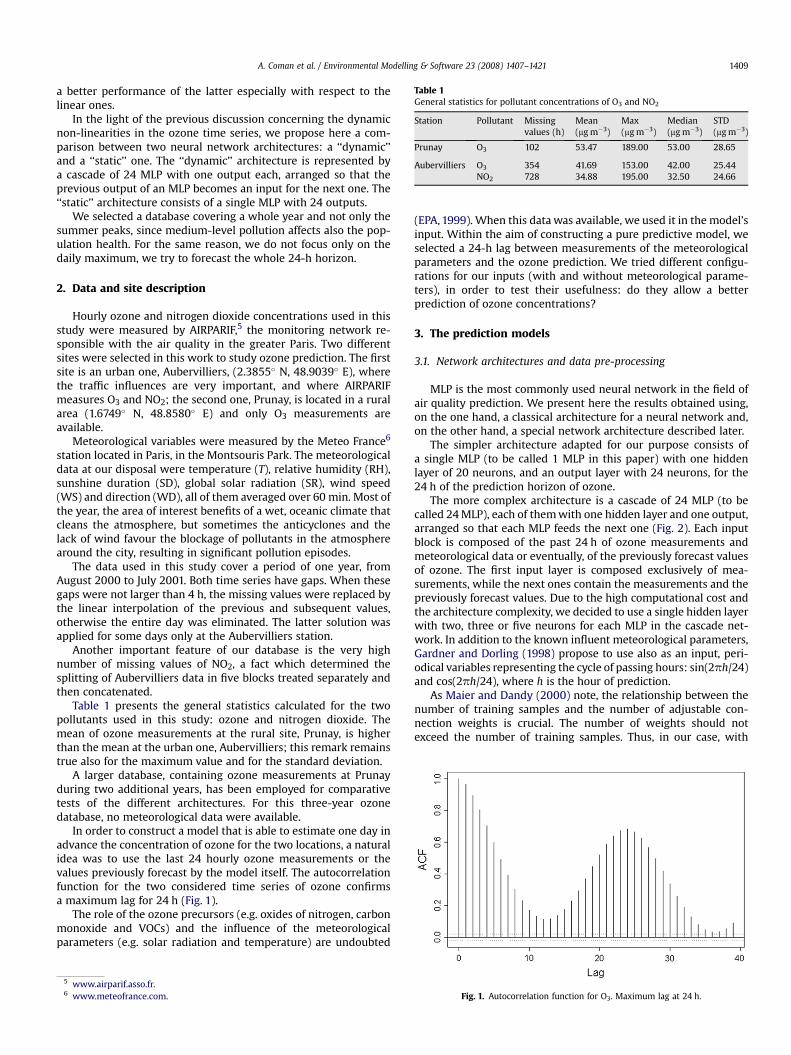
Table 1General statistics for pollutant concentrations of O3 and NO2

Station Pollutant Missingvalues (h)

Mean(mg m�3)

Max(mg m�3)

Median(mg m�3)

STD(mg m�3)

Prunay O3 102 53.47 189.00 53.00 28.65

Aubervilliers O3 354 41.69 153.00 42.00 25.44NO2 728 34.88 195.00 32.50 24.66

A. Coman et al. / Environmental Modelling & Software 23 (2008) 1407–1421 1409

a better performance of the latter especially with respect to thelinear ones.

In the light of the previous discussion concerning the dynamicnon-linearities in the ozone time series, we propose here a com-parison between two neural network architectures: a ‘‘dynamic’’and a ‘‘static’’ one. The ‘‘dynamic’’ architecture is represented bya cascade of 24 MLP with one output each, arranged so that theprevious output of an MLP becomes an input for the next one. The‘‘static’’ architecture consists of a single MLP with 24 outputs.

We selected a database covering a whole year and not only thesummer peaks, since medium-level pollution affects also the pop-ulation health. For the same reason, we do not focus only on thedaily maximum, we try to forecast the whole 24-h horizon.

2. Data and site description

Hourly ozone and nitrogen dioxide concentrations used in thisstudy were measured by AIRPARIF,5 the monitoring network re-sponsible with the air quality in the greater Paris. Two differentsites were selected in this work to study ozone prediction. The firstsite is an urban one, Aubervilliers, (2.3855� N, 48.9039� E), wherethe traffic influences are very important, and where AIRPARIFmeasures O3 and NO2; the second one, Prunay, is located in a ruralarea (1.6749� N, 48.8580� E) and only O3 measurements areavailable.

Meteorological variables were measured by the Meteo France6

station located in Paris, in the Montsouris Park. The meteorologicaldata at our disposal were temperature (T), relative humidity (RH),sunshine duration (SD), global solar radiation (SR), wind speed(WS) and direction (WD), all of them averaged over 60 min. Most ofthe year, the area of interest benefits of a wet, oceanic climate thatcleans the atmosphere, but sometimes the anticyclones and thelack of wind favour the blockage of pollutants in the atmospherearound the city, resulting in significant pollution episodes.

The data used in this study cover a period of one year, fromAugust 2000 to July 2001. Both time series have gaps. When thesegaps were not larger than 4 h, the missing values were replaced bythe linear interpolation of the previous and subsequent values,otherwise the entire day was eliminated. The latter solution wasapplied for some days only at the Aubervilliers station.

Another important feature of our database is the very highnumber of missing values of NO2, a fact which determined thesplitting of Aubervilliers data in five blocks treated separately andthen concatenated.

Table 1 presents the general statistics calculated for the twopollutants used in this study: ozone and nitrogen dioxide. Themean of ozone measurements at the rural site, Prunay, is higherthan the mean at the urban one, Aubervilliers; this remark remainstrue also for the maximum value and for the standard deviation.

A larger database, containing ozone measurements at Prunayduring two additional years, has been employed for comparativetests of the different architectures. For this three-year ozonedatabase, no meteorological data were available.

In order to construct a model that is able to estimate one day inadvance the concentration of ozone for the two locations, a naturalidea was to use the last 24 hourly ozone measurements or thevalues previously forecast by the model itself. The autocorrelationfunction for the two considered time series of ozone confirmsa maximum lag for 24 h (Fig. 1).

The role of the ozone precursors (e.g. oxides of nitrogen, carbonmonoxide and VOCs) and the influence of the meteorologicalparameters (e.g. solar radiation and temperature) are undoubted

5 www.airparif.asso.fr.6 www.meteofrance.com.

(EPA, 1999). When this data was available, we used it in the model’sinput. Within the aim of constructing a pure predictive model, weselected a 24-h lag between measurements of the meteorologicalparameters and the ozone prediction. We tried different configu-rations for our inputs (with and without meteorological parame-ters), in order to test their usefulness: do they allow a betterprediction of ozone concentrations?

3. The prediction models

3.1. Network architectures and data pre-processing

MLP is the most commonly used neural network in the field ofair quality prediction. We present here the results obtained using,on the one hand, a classical architecture for a neural network and,on the other hand, a special network architecture described later.

The simpler architecture adapted for our purpose consists ofa single MLP (to be called 1 MLP in this paper) with one hiddenlayer of 20 neurons, and an output layer with 24 neurons, for the24 h of the prediction horizon of ozone.

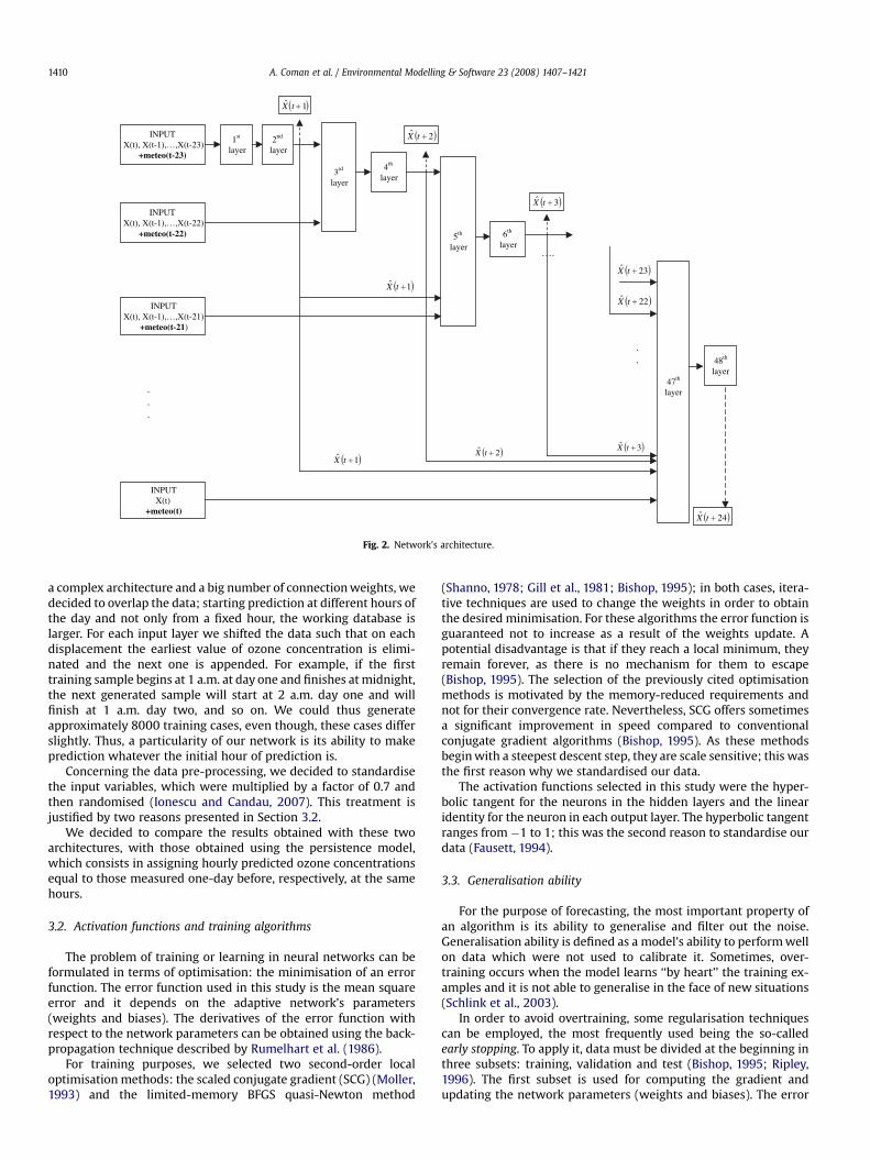
The more complex architecture is a cascade of 24 MLP (to becalled 24 MLP), each of them with one hidden layer and one output,arranged so that each MLP feeds the next one (Fig. 2). Each inputblock is composed of the past 24 h of ozone measurements andmeteorological data or eventually, of the previously forecast valuesof ozone. The first input layer is composed exclusively of mea-surements, while the next ones contain the measurements and thepreviously forecast values. Due to the high computational cost andthe architecture complexity, we decided to use a single hidden layerwith two, three or five neurons for each MLP in the cascade net-work. In addition to the known influent meteorological parameters,Gardner and Dorling (1998) propose to use also as an input, peri-odical variables representing the cycle of passing hours: sin(2ph/24)and cos(2ph/24), where h is the hour of prediction.

As Maier and Dandy (2000) note, the relationship between thenumber of training samples and the number of adjustable con-nection weights is crucial. The number of weights should notexceed the number of training samples. Thus, in our case, with

Fig. 1. Autocorrelation function for O3. Maximum lag at 24 h.

INPUT X(t), X(t-1),…,X(t-23)

+meteo(t-23)

1st

layer2nd

layer

3rd

layer

INPUT X(t), X(t-1),…,X(t-22)

+meteo(t-22)

4th

layer

2ˆ tX

INPUTX(t), X(t-1),…,X(t-21)

+meteo(t-21)

1ˆ tX

5th

layer

6th

layer

3ˆ tX

1ˆ tX

47th

layer

48th

layer

24ˆ tX

22ˆ tX

23ˆ tX

INPUTX(t)

+meteo(t)

.

.

.

.

.

….

1ˆ tX

3ˆ tX2ˆ tX

Fig. 2. Network’s architecture.

A. Coman et al. / Environmental Modelling & Software 23 (2008) 1407–14211410

a complex architecture and a big number of connection weights, wedecided to overlap the data; starting prediction at different hours ofthe day and not only from a fixed hour, the working database islarger. For each input layer we shifted the data such that on eachdisplacement the earliest value of ozone concentration is elimi-nated and the next one is appended. For example, if the firsttraining sample begins at 1 a.m. at day one and finishes at midnight,the next generated sample will start at 2 a.m. day one and willfinish at 1 a.m. day two, and so on. We could thus generateapproximately 8000 training cases, even though, these cases differslightly. Thus, a particularity of our network is its ability to makeprediction whatever the initial hour of prediction is.

Concerning the data pre-processing, we decided to standardisethe input variables, which were multiplied by a factor of 0.7 andthen randomised (Ionescu and Candau, 2007). This treatment isjustified by two reasons presented in Section 3.2.

We decided to compare the results obtained with these twoarchitectures, with those obtained using the persistence model,which consists in assigning hourly predicted ozone concentrationsequal to those measured one-day before, respectively, at the samehours.

3.2. Activation functions and training algorithms

The problem of training or learning in neural networks can beformulated in terms of optimisation: the minimisation of an errorfunction. The error function used in this study is the mean squareerror and it depends on the adaptive network’s parameters(weights and biases). The derivatives of the error function withrespect to the network parameters can be obtained using the back-propagation technique described by Rumelhart et al. (1986).

For training purposes, we selected two second-order localoptimisation methods: the scaled conjugate gradient (SCG) (Moller,1993) and the limited-memory BFGS quasi-Newton method

(Shanno, 1978; Gill et al., 1981; Bishop, 1995); in both cases, itera-tive techniques are used to change the weights in order to obtainthe desired minimisation. For these algorithms the error function isguaranteed not to increase as a result of the weights update. Apotential disadvantage is that if they reach a local minimum, theyremain forever, as there is no mechanism for them to escape(Bishop, 1995). The selection of the previously cited optimisationmethods is motivated by the memory-reduced requirements andnot for their convergence rate. Nevertheless, SCG offers sometimesa significant improvement in speed compared to conventionalconjugate gradient algorithms (Bishop, 1995). As these methodsbegin with a steepest descent step, they are scale sensitive; this wasthe first reason why we standardised our data.

The activation functions selected in this study were the hyper-bolic tangent for the neurons in the hidden layers and the linearidentity for the neuron in each output layer. The hyperbolic tangentranges from �1 to 1; this was the second reason to standardise ourdata (Fausett, 1994).

3.3. Generalisation ability

For the purpose of forecasting, the most important property ofan algorithm is its ability to generalise and filter out the noise.Generalisation ability is defined as a model’s ability to perform wellon data which were not used to calibrate it. Sometimes, over-training occurs when the model learns ‘‘by heart’’ the training ex-amples and it is not able to generalise in the face of new situations(Schlink et al., 2003).

In order to avoid overtraining, some regularisation techniquescan be employed, the most frequently used being the so-calledearly stopping. To apply it, data must be divided at the beginning inthree subsets: training, validation and test (Bishop, 1995; Ripley,1996). The first subset is used for computing the gradient andupdating the network parameters (weights and biases). The error

A. Coman et al. / Environmental Modelling & Software 23 (2008) 1407–1421 1411

calculated on the second one is monitored during the trainingprocess; when the network begins to overfit the data, the error onthe validation set begins to rise; this is the moment when trainingis stopped and the network parameters at the minimum of thevalidation error are returned. Finally, the third set (the test set) isused to evaluate the model performance (Nunnari et al., 2004).

In our study, the training set was fixed at 60% of all availabledata, while the validation and test sets, at 20% each one. Thissplitting was performed after the randomisation.

3.4. Performance indices

For a good evaluation of the results obtained with different ar-chitectures, we calculated different statistical parameters for eachhour of the prediction horizon, but also some global indices for theentire test set.

Among the classical statistical criteria, we evaluated the de-termination coefficient R2, the root mean square error RMSE,the mean absolute error MAE, and the mean bias error MBE; allthese indices measure residual errors and give a global idea of thedifference between observed and modelled values. Their formulasare reminded in Eqs. (1)–(4):

R ¼

ffiffiffiffiffiffiffiffiffiffiffiffiffiffiffiffiffiffiffiffiffiffiffiffiffiffiffiffiffiffiffiffiffiffiffiffiffiffiffiffiffiffiffiffiffiffiffiffiffiffiffiffiffiffiffiffiffiffiffiffiffiffiffiffiffiffiffiffiffiffiPni¼1ðOi � OÞ2�

Pni¼1ðOi � PiÞ2Pn

i¼1ðOi � OÞ2

vuut (1)

ffiffiffiffiffiffiffiffiffiffiffiffiffiffiffiffiffiffiffiffiffiffiffiffiffiffiffiffiffiffiffin

vu

n

Xi¼1

ðOi � PiÞ2ut (2)

1Xn

MAE ¼n

i¼1

jPi � Oij (3)

1Xn

MBE ¼n

i¼1

ðPi � OiÞ (4)

where Pi and Oi are the predicted and observed concentrations, and�O represents the observation mean.

In addition, we determined the index of agreement d2 (Will-mott, 1982), which is a relative measure expressing the degree towhich predictions are error-free (Gardner and Dorling, 2000), andwhich allows the comparison of different models using differentdata sets (Schlink et al., 2003):

d2 ¼ 1�Pn

i¼1jPi � Oij2Pni¼1ðjPi � Oj þ jOi � OjÞ2

(5)

Other indices mentioned in this study are the Normalised MeanSquare Error (NMSE):

Table 2Global indices calculated on the entire horizon (cf. Section 3.4) on the test set for the sim

Inputs (number): description Training algorithm Mean (mg m�3) STD (mg

(24): O3 BFGS 32.05 28.85SCG 31.41 27.80

(26): O3, T, NO2 BFGS 29.85 27.43SCG 30.84 27.71

(28): O3, T, RH, SR, NO2 BFGS 30.13 27.24SCG 30.81 27.84

(30): O3, T, RH, SR, SD, WS, NO2 BFGS 29.83 26.74SCG 30.50 26.90

Abbreviations: T – temperature, RH – relative humidity, SR – solar radiation, SD – sunshinprediction time; O3 – ozone concentrations during all the 24 h before the prediction time;Fletcher, Goldfarb and Shanno algorithm); SCG – scaled conjugate gradient.

NMSE ¼1nPn

i¼1ðOi � PiÞ2

O� P(6)

the factor FA2, which gives the percentage of forecast cases in whichthe values of the ratio O/P are in the range [0.5, 2], the FractionalBias (FB):

FB ¼ 2O� P

Oþ P(7)

and the Fractional Variance (FV):

FV ¼ 2s2

O � s2P

s2O þ s2

P

(8)

with the same meaning for O and P.For the prediction exceedances, Schlink et al. (2006) propose

three specific indices. The first one, the true positive rate (TPR),corresponds to the fraction of correctly predicted exceedances andit can be defined as

TPR ¼ A=M (9)

where A represents the correctly predicted exceedances and M allobserved exceedances, while the second one, the false positive rate(FPR), can be achieved according to the formula:

FPR ¼ ðF � AÞ=ðN �MÞ (10)

where N is the total number of days considered and F all the pre-dicted exceedances. Finally, the success index SI is obtained bycombining the previous rates:

SI ¼ TPR � FPR (11)

4. Results and discussion

4.1. Results at Aubervilliers

For the site of Aubervilliers we present eight ranges of statistics,for each simulation using the 24 MLP model, in terms of globalindices calculated on the test set (Table 2).

At this site we had a major problem with gaps in the NO2 timeseries. Although O3 gaps were not so big, we decided to eliminatemany days in order to obtain in this way a common base for the O3

measurements, NO2 concentrations and meteorological variables.We performed eight simulations using two training algorithms(BFGS and SCG), and different combinations of meteorologicalparameters together with the pollutant concentrations as inputs.

The first two simulations were performed using only O3 mea-surements or forecast values, but no meteorological predictors

ulations performed at Aubervilliers using the 24 MLP model

m�3) RMSE (mg m�3) MAE (mg m�3) MBE (mg m�3) d2 R2

19.55 14.87 0.46 0.83 0.5419.01 14.51 0.17 0.83 0.53

18.48 14.07 �0.05 0.84 0.5518.49 14.14 0.42 0.84 0.55

17.87 13.66 0.08 0.85 0.5718.32 13.90 0.25 0.85 0.57

17.62 13.54 �0.01 0.85 0.5718.00 13.87 0.03 0.85 0.55

e duration, WS – wind speed, NO2 – nitrogen dioxide, all of them at 24 h before thet is a function of the prediction hour (h) (t¼ 2ph/24); BFGS – quasi-Newton (Broyden,

A. Coman et al. / Environmental Modelling & Software 23 (2008) 1407–14211412

(24 inputs). For the next ones, we added at these 24 inputs, 1 andthen 3 meteorological parameters: temperature T, relative humid-ity RH, global solar radiation SR plus the NO2 measurements.Occasionally used predictors were sunshine duration SD and windspeed WS (30 inputs).

A good compromise between the network size and the selectedpredictors in the forecasting process shows that the best results interms of index of agreement and determination coefficient areobtained using the BFGS training algorithm and the following in-puts: 24 ozone concentrations, the 3 meteorological parametersearlier mentioned and the NO2 measurements (cf. Table 2).

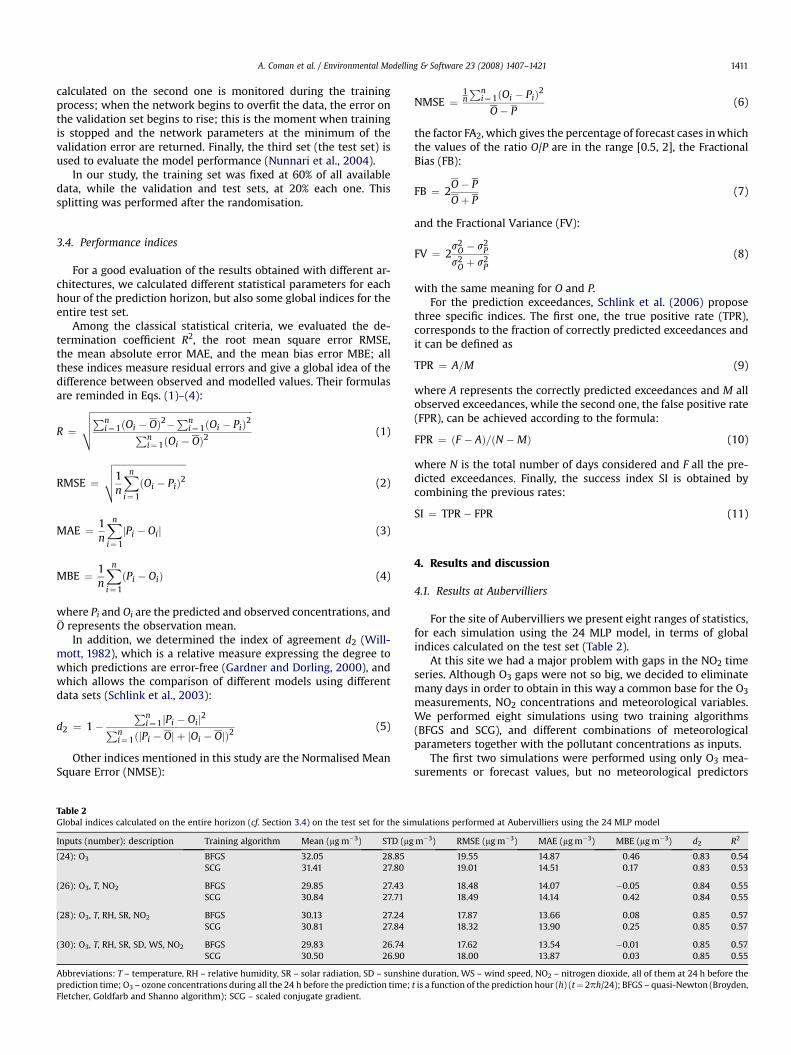
On the prediction horizon, the best results varied from R2¼ 0.89,RMSE¼ 9.03 mg m�3, d2¼ 0.97, MAE¼ 6.51 mg m�3 for 1 h ahead, upto R2¼ 0.54, RMSE¼ 18.95 mg m�3, d2¼ 0.84, MAE¼ 14.88 mg m�3

for 24 h ahead. These variations are illustrated for the RMSE and R2

statistics, on Fig. 3.Nevertheless, we can notice that the applied models exhibit

similar levels of performance. This is obvious if we analyse theFig. 3, where we represented two performance indices (R2 andRMSE) for the worst (24 inputs) and, respectively, best (28 inputs)

Fig. 3. Performance indices (cf. Section 3.4) on the test set for the worst (RMSE (a), R2 (a)) anentire prediction horizon using the 24 MLP model.

simulations performed at this station. We observed a normal evo-lution for R2 and RMSE, the two indices presented in Fig. 3: the firstone is decreasing and the second one is increasing gradually withthe prediction horizon.

The exogenous variables, i.e. meteorological parameters andNO2 concentration, do not increase sensibly the model perfor-mance. It is probably that their influence is not crucial for ozoneprediction when there is no high variation from one day to another;such strong variations appear usually in the case of importantpollution peaks, but there are very few such examples within ourdatabase. Another plausible explanation resides in the fact that themeteorological parameters are monitored by a station located inthe centre of Paris, while the Aubervilliers station is located in Parisoutskirts, rather far from it; thus the meteorological parametersused are not so representative as if they were measured at the samelocation or in its vicinity.

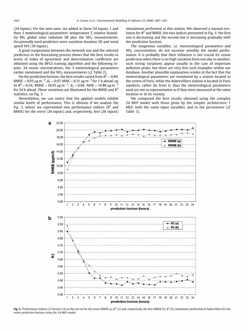
We compared the best results obtained using the complex24 MLP model with those given by the simpler architecture, 1MLP, with the same input variables, and to the persistence (cf.Table 3).

d, respectively, the best (RMSE (b), R2 (b)) simulations performed at Aubervilliers for the

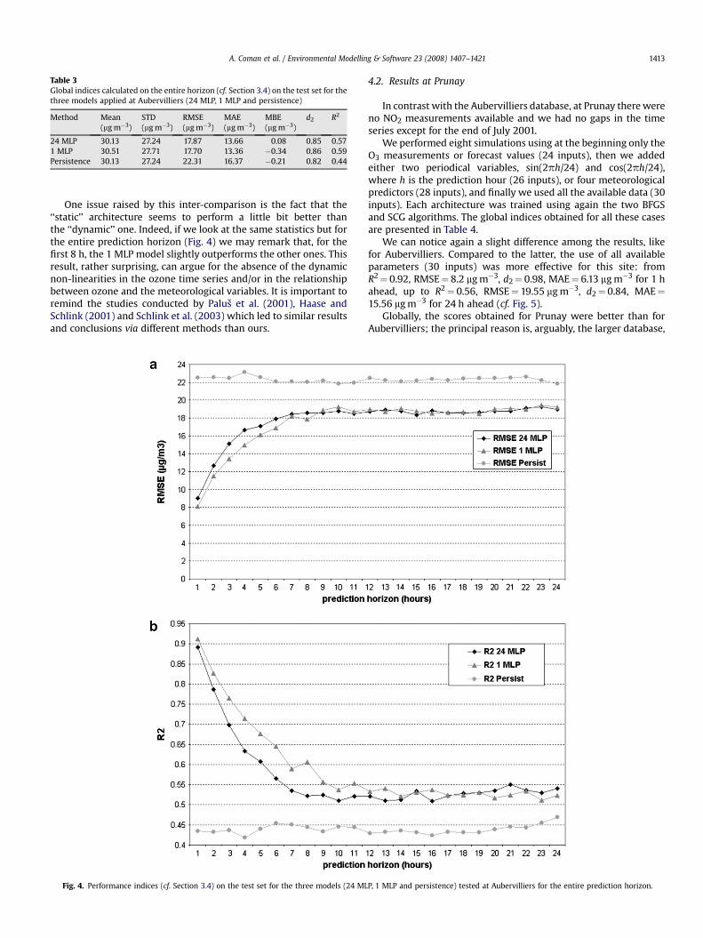
Table 3Global indices calculated on the entire horizon (cf. Section 3.4) on the test set for thethree models applied at Aubervilliers (24 MLP, 1 MLP and persistence)

Method Mean(mg m�3)

STD(mg m�3)

RMSE(mg m�3)

MAE(mg m�3)

MBE(mg m�3)

d2 R2

24 MLP 30.13 27.24 17.87 13.66 0.08 0.85 0.571 MLP 30.51 27.71 17.70 13.36 �0.34 0.86 0.59Persistence 30.13 27.24 22.31 16.37 �0.21 0.82 0.44

A. Coman et al. / Environmental Modelling & Software 23 (2008) 1407–1421 1413

One issue raised by this inter-comparison is the fact that the‘‘static’’ architecture seems to perform a little bit better thanthe ‘‘dynamic’’ one. Indeed, if we look at the same statistics but forthe entire prediction horizon (Fig. 4) we may remark that, for thefirst 8 h, the 1 MLP model slightly outperforms the other ones. Thisresult, rather surprising, can argue for the absence of the dynamicnon-linearities in the ozone time series and/or in the relationshipbetween ozone and the meteorological variables. It is important toremind the studies conducted by Palus et al. (2001), Haase andSchlink (2001) and Schlink et al. (2003) which led to similar resultsand conclusions via different methods than ours.

Fig. 4. Performance indices (cf. Section 3.4) on the test set for the three models (24 ML

4.2. Results at Prunay

In contrast with the Aubervilliers database, at Prunay there wereno NO2 measurements available and we had no gaps in the timeseries except for the end of July 2001.

We performed eight simulations using at the beginning only theO3 measurements or forecast values (24 inputs), then we addedeither two periodical variables, sin(2ph/24) and cos(2ph/24),where h is the prediction hour (26 inputs), or four meteorologicalpredictors (28 inputs), and finally we used all the available data (30inputs). Each architecture was trained using again the two BFGSand SCG algorithms. The global indices obtained for all these casesare presented in Table 4.

We can notice again a slight difference among the results, likefor Aubervilliers. Compared to the latter, the use of all availableparameters (30 inputs) was more effective for this site: fromR2¼ 0.92, RMSE¼ 8.2 mg m�3, d2¼ 0.98, MAE¼ 6.13 mg m�3 for 1 hahead, up to R2¼ 0.56, RMSE¼ 19.55 mg m�3, d2¼ 0.84, MAE¼15.56 mg m�3 for 24 h ahead (cf. Fig. 5).

Globally, the scores obtained for Prunay were better than forAubervilliers; the principal reason is, arguably, the larger database,

P, 1 MLP and persistence) tested at Aubervilliers for the entire prediction horizon.

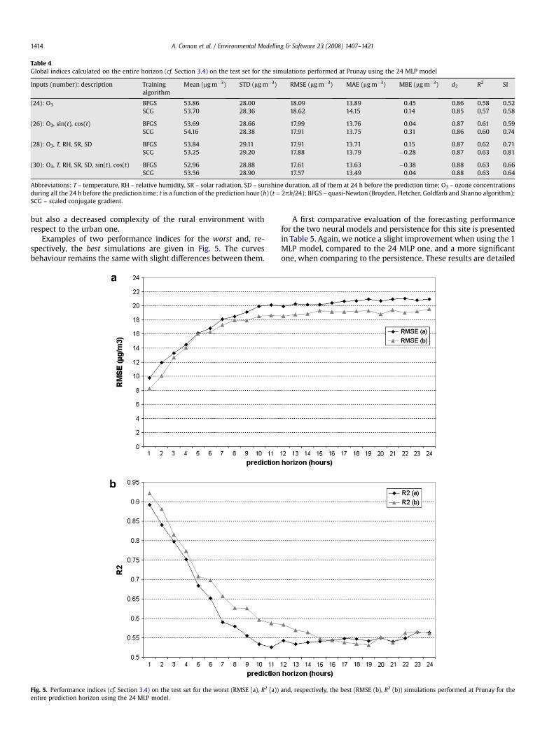
Table 4Global indices calculated on the entire horizon (cf. Section 3.4) on the test set for the simulations performed at Prunay using the 24 MLP model

Inputs (number): description Trainingalgorithm

Mean (mg m�3) STD (mg m�3) RMSE (mg m�3) MAE (mg m�3) MBE (mg m�3) d2 R2 SI

(24): O3 BFGS 53.86 28.00 18.09 13.89 0.45 0.86 0.58 0.52SCG 53.70 28.36 18.62 14.15 0.14 0.85 0.57 0.58

(26): O3, sin(t), cos(t) BFGS 53.69 28.66 17.99 13.76 0.04 0.87 0.61 0.59SCG 54.16 28.38 17.91 13.75 0.31 0.86 0.60 0.74

(28): O3, T, RH, SR, SD BFGS 53.84 29.11 17.91 13.71 0.15 0.87 0.62 0.71SCG 53.25 29.20 17.88 13.79 �0.28 0.87 0.63 0.81

(30): O3, T, RH, SR, SD, sin(t), cos(t) BFGS 52.96 28.88 17.61 13.63 �0.38 0.88 0.63 0.66SCG 53.56 28.90 17.57 13.49 0.04 0.88 0.63 0.64

Abbreviations: T – temperature, RH – relative humidity, SR – solar radiation, SD – sunshine duration, all of them at 24 h before the prediction time; O3 – ozone concentrationsduring all the 24 h before the prediction time; t is a function of the prediction hour (h) (t¼ 2ph/24); BFGS – quasi-Newton (Broyden, Fletcher, Goldfarb and Shanno algorithm);SCG – scaled conjugate gradient.

A. Coman et al. / Environmental Modelling & Software 23 (2008) 1407–14211414

but also a decreased complexity of the rural environment withrespect to the urban one.

Examples of two performance indices for the worst and, re-spectively, the best simulations are given in Fig. 5. The curvesbehaviour remains the same with slight differences between them.

Fig. 5. Performance indices (cf. Section 3.4) on the test set for the worst (RMSE (a), R2 (a))entire prediction horizon using the 24 MLP model.

A first comparative evaluation of the forecasting performancefor the two neural models and persistence for this site is presentedin Table 5. Again, we notice a slight improvement when using the 1MLP model, compared to the 24 MLP one, and a more significantone, when comparing to the persistence. These results are detailed

and, respectively, the best (RMSE (b), R2 (b)) simulations performed at Prunay for the

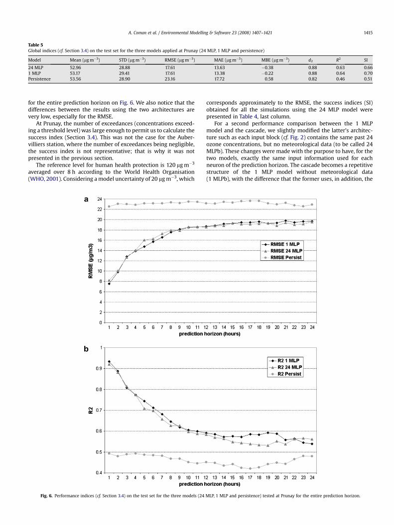
Table 5Global indices (cf. Section 3.4) on the test set for the three models applied at Prunay (24 MLP, 1 MLP and persistence)

Model Mean (mg m�3) STD (mg m�3) RMSE (mg m�3) MAE (mg m�3) MBE (mg m�3) d2 R2 SI

24 MLP 52.96 28.88 17.61 13.63 �0.38 0.88 0.63 0.661 MLP 53.17 29.41 17.61 13.38 �0.22 0.88 0.64 0.70Persistence 53.56 28.90 23.16 17.72 0.58 0.82 0.46 0.51

A. Coman et al. / Environmental Modelling & Software 23 (2008) 1407–1421 1415

for the entire prediction horizon on Fig. 6. We also notice that thedifferences between the results using the two architectures arevery low, especially for the RMSE.

At Prunay, the number of exceedances (concentrations exceed-ing a threshold level) was large enough to permit us to calculate thesuccess index (Section 3.4). This was not the case for the Auber-villiers station, where the number of exceedances being negligible,the success index is not representative; that is why it was notpresented in the previous section.

The reference level for human health protection is 120 mg m�3

averaged over 8 h according to the World Health Organisation(WHO, 2001). Considering a model uncertainty of 20 mg m�3, which

Fig. 6. Performance indices (cf. Section 3.4) on the test set for the three models (24

corresponds approximately to the RMSE, the success indices (SI)obtained for all the simulations using the 24 MLP model werepresented in Table 4, last column.

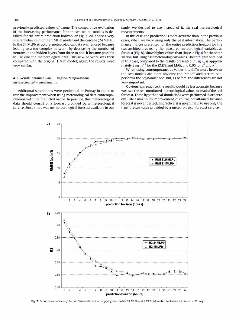
For a second performance comparison between the 1 MLPmodel and the cascade, we slightly modified the latter’s architec-ture such as each input block (cf. Fig. 2) contains the same past 24ozone concentrations, but no meteorological data (to be called 24MLPb). These changes were made with the purpose to have, for thetwo models, exactly the same input information used for eachneuron of the prediction horizon. The cascade becomes a repetitivestructure of the 1 MLP model without meteorological data(1 MLPb), with the difference that the former uses, in addition, the

MLP, 1 MLP and persistence) tested at Prunay for the entire prediction horizon.

A. Coman et al. / Environmental Modelling & Software 23 (2008) 1407–14211416

previously predicted values of ozone. The comparative evaluationof the forecasting performance for the two neural models is de-tailed, for the entire prediction horizon, on Fig. 7. We notice a verysimilar behaviour for the 1 MLPb model and the cascade (24 MLPb).In the 24 MLPb structure, meteorological data was ignored becauseleading to a too complex network; by decreasing the number ofneurons in the hidden layers from three to one, it became possibleto use also the meteorological data. This new network was thencompared with the original 1 MLP model; again, the results werevery similar.

4.3. Results obtained when using contemporaneousmeteorological measurements

Additional simulations were performed at Prunay in order totest the improvement when using meteorological data contempo-raneous with the predicted ozone. In practice, this meteorologicaldata should consist of a forecast provided by a meteorologicalservice. Since there was no meteorological forecast available in our

Fig. 7. Performance indices (cf. Section 3.4) on the test set applying two mo

study, we decided to use instead of it, the real meteorologicalmeasurements.

In this case, the prediction is more accurate than in the previouscases, when we were using only the past information. The perfor-mance indices presented for the entire prediction horizon for thetwo architectures using the measured meteorological variables asforecast (Fig. 8), show higher values than those in Fig. 6 for the samestation, but using past meteorological values. The total gain obtainedin this case, compared to the results presented in Fig. 6, is approxi-mately 2 mg m�3 for the RMSE and MAE, and 0.05 for d2 and R2.

When using contemporaneous values, the differences betweenthe two models are more obvious: the ‘‘static’’ architecture out-performs the ‘‘dynamic’’ one, but, as before, the differences are notvery important.

Obviously, in practice, the results would be less accurate, becausewe used the real monitored meteorological values instead of the realforecast. These hypothetical simulations were performed in order toevaluate a maximum improvement, of course, not attained, becauseforecast is never perfect. In practice, it is meaningful to use only thetrue forecast value provided by a meteorological forecast service.

dels 24 MLPb and 1 MLPb (described in Section 4.2) tested at Prunay.

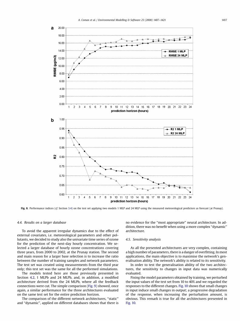
Fig. 8. Performance indices (cf. Section 3.4) on the test set applying two models 1 MLP and 24 MLP using the measured meteorological predictors as forecast (at Prunay).

A. Coman et al. / Environmental Modelling & Software 23 (2008) 1407–1421 1417

4.4. Results on a larger database

To avoid the apparent irregular dynamics due to the effect ofexternal covariates, i.e. meteorological parameters and other pol-lutants, we decided to study also the univariate time series of ozonefor the prediction of the next-day hourly concentration. We se-lected a larger database of hourly ozone concentrations coveringthree years, from 2000 to 2002, at the Prunay station. The secondand main reason for a larger base selection is to increase the ratiobetween the number of training samples and network parameters.The test set was created using measurements from the third yearonly; this test set was the same for all the performed simulations.

The models tested here are those previously presented inSection 4.2, 1 MLPb and 24 MLPb, and, in addition, a modifiedarchitecture derived from the 24 MLPb, where all the feedbackconnections were cut. The simple comparison (Fig. 9) showed, onceagain, a similar performance for the three architectures evaluatedon the same test set for the entire prediction horizon.

The comparison of the different network architectures, ‘‘static’’and ‘‘dynamic’’, applied on different databases shows that there is

no evidence for the ‘‘most appropriate’’ neural architecture. In ad-dition, there was no benefit when using a more complex ‘‘dynamic’’architecture.

4.5. Sensitivity analysis

As all the presented architectures are very complex, containinga high number of parameters, there is a danger of overfitting. In mostapplications, the main objective is to maximise the network’s gen-eralisation ability. The network’s ability is related to its sensitivity.

In order to test the generalisation ability of the two architec-tures, the sensitivity to changes in input data was numericallyevaluated.

Fixing the model parameters obtained by training, we perturbedthe input values of the test set from 10 to 40% and we regarded theresponses to the different changes. Fig. 10 shows that small changesin input induce small changes in output; a progressive degradationof the response, when increasing the perturbation amount, isobvious. This remark is true for all the architectures presented inFig. 10.

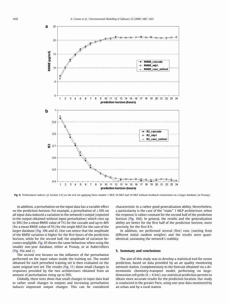
Fig. 9. Performance indices (cf. Section 3.4) on the test set applying three models 1 MLP, 24 MLP and 24 MLP without feedback connections on a larger database (at Prunay).

A. Coman et al. / Environmental Modelling & Software 23 (2008) 1407–14211418

In addition, a perturbation on the input data has a variable effecton the prediction horizon. For example, a perturbation of �10% onall input data induced a variation in the network’s output (reportedto the output obtained without input perturbation) which rises upto 30% (for a mean RMSE value of 7%) for the cascade and up to 40%(for a mean RMSE value of 5%) for the single MLP, for the case of thelarger database (Fig. 10b and d). One can notice that the amplitudeof the RMSE variation is higher for the first hours of the predictionhorizon, while for the second half, the amplitude of variation be-comes negligible. Fig. 10 shows the same behaviour when using thesmaller one-year database, either at Prunay, or at Aubervilliers(Fig. 10a and c).

The second test focuses on the influence of the perturbationperformed on the input values inside the training set. The modelobtained for each perturbed training set is then evaluated on thesame original test set. The results (Fig. 11) show small changes inresponses provided by the two architectures obtained from anamount of perturbation rising up to 50%.

Globally, these tests show that small changes in input data leadto rather small changes in outputs and increasing perturbationinduces important output changes. This can be considered

characteristic to a rather good generalisation ability. Nevertheless,a particularity is the case of the ‘‘static’’ 1 MLP architecture, whenthe response is rather constant for the second half of the predictionhorizon (Fig. 10d). In general, the results and the generalisationability are better for the first half of the prediction horizon, moreprecisely, for the first 8 h.

In addition, we performed several (five) runs (starting fromdifferent initial random weights) and the results were quasi-identical, sustaining the network’s stability.

5. Summary and conclusions

The aim of this study was to develop a statistical tool for ozoneprediction, based on data provided by an air quality monitoringnetwork station. Complementary to the forecast obtained via a de-terministic chemistry-transport model, performing on large-dimension cell grids (6� 6 km), our statistical prediction permits toobtain more accurate results for the prediction location. Our studyis conducted in the greater Paris, using one-year data monitored byan urban and by a rural station.

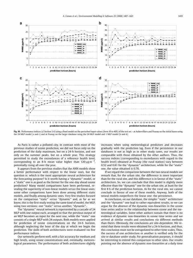
Fig. 10. Performance indices (cf. Section 3.4) using a fixed model on the perturbed input values (form 10 to 40%) of the test set – at Aubervilliers and Prunay on the initial bases usingthe 24 MLP model (a and c) and at Prunay on the larger database using the 24 MLP model and 1 MLP model (b and d).

A. Coman et al. / Environmental Modelling & Software 23 (2008) 1407–1421 1419

As Paris is rather a polluted city, in contrast with most of theprevious studies of ozone prediction, we did not focus only on theprediction of the daily maximum, but on a 24-h horizon, and notonly on the summer peaks, but on a whole year. This strategypermitted to study the exceedances of a reference health level,corresponding to an 8-h mean value higher than 120 mg m�3,potentially rising all over the year.

It appears from the previous studies that the ANN models showa better performance with respect to the linear ones, but thequestion is: which is the most appropriate neural architecture forthe forecasting purpose? Is it worth having a ‘‘dynamic’’ model, ora ‘‘static’’ one is as good as the former for the one-day ahead ozoneprediction? Many model comparisons have been performed, re-vealing the superiority of non-linear models versus the linear ones;some other comparisons have been done among different staticmodels, and finally among dynamic ones. Very few studies focusedon the comparison ‘‘static’’ versus ‘‘dynamic’’ and, as far as weknow, this is the first study testing the same kind of model, the MLP,using two versions: one ‘‘static’’ versus another, ‘‘dynamic’’.

The ‘‘dynamic’’ neural network is represented by a cascade of 24MLP with one output each, arranged so that the previous output ofan MLP becomes an input for the next one, while the ‘‘static’’ oneconsists of a single MLP with 24 outputs. Both models were appliedfor prediction of ozone concentrations on the 24-h horizon,although neglecting the hour of the day at which we begin theprediction. The skills of both architectures were evaluated via fiveperformance indices.

Our networks perform well, with a fair accuracy for medium andhigh levels, using ozone concentrations and, eventually, meteoro-logical parameters. The performance of both architectures slightly

increases when using meteorological predictors and decreasesgradually with the prediction lag. Even if the persistence in ourdatabases is not as high as in other study cases, our results arecomparable with those obtained by the other authors. Thus, thesuccess indices (corresponding to exceedances with regard to thehealth level) obtained at Prunay (the rural station) vary between0.52 and 0.81 for the ‘‘dynamic’’ architecture, while for the ‘‘static’’one, the value obtained is 0.70.

If we regard the comparison between the two neural models weremark that, for the urban site, the difference is more importantthan for the rural site, and this difference is in favour of the ‘‘static’’architecture. So, we can conclude that this model is slightly moreeffective than the ‘‘dynamic’’ one for the urban site, at least for thefirst 8 h of the prediction horizon. As for the rural site, we cannotconclude in favour of one of these models. Anyway, both of theneural models outperform the linear one: the persistence.

In conclusion, on our database, the simpler ‘‘static’’ architectureand the ‘‘dynamic’’ one lead to rather equivalent results, so we canargue for the absence of the dynamic non-linearities in the ozonetime series and/or in the relationship between ozone and the me-teorological variables. Some other authors sustain that there is noevidence of dynamic non-linearities in ozone time series and wearrived at similar results and conclusions via different methodsthan theirs. Obviously, the conclusions are site-dependent. We re-mind that these results were obtained for a 24-h horizon, and thus,this conclusion must not be extrapolated to other time scales. Thus,the success of one architecture or another is verified only for thesite or database under study. For generalisation purposes, it shouldbe interesting to extend this comparison to other sites. Our resultspointing out the absence of dynamic non-linearities at a daily time

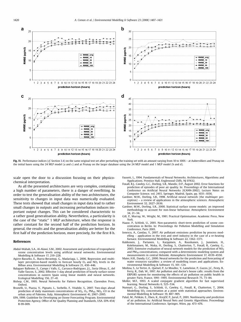
Fig. 11. Performance indices (cf. Section 3.4) on the same original test set after perturbing the training set with an amount varying from 10 to 100% – at Aubervilliers and Prunay onthe initial bases using the 24 MLP model (a and c) and at Prunay on the larger database using the 24 MLP model and 1 MLP model (b and d).

A. Coman et al. / Environmental Modelling & Software 23 (2008) 1407–14211420

scale open the door to a discussion focusing on their physico-chemical interpretation.

As all the presented architectures are very complex, containinga high number of parameters, there is a danger of overfitting. Inorder to test the generalisation ability of the two architectures, thesensitivity to changes in input data was numerically evaluated.These tests showed that small changes in input data lead to rathersmall changes in outputs and increasing perturbation induces im-portant output changes. This can be considered characteristic toa rather good generalisation ability. Nevertheless, a particularity isthe case of the ‘‘static’’ 1 MLP architecture, when the response israther constant for the second half of the prediction horizon. Ingeneral, the results and the generalisation ability are better for thefirst half of the prediction horizon, more precisely, for the first 8 h.

References

Abdul-Wahab, S.A., Al-Alawi, S.M., 2002. Assessment and prediction of troposphericozone concentration levels using artificial neural networks. EnvironmentalModelling & Software 17, 219–228.

Agirre-Basurko, E., Ibarra-Berastegi, G., Madariaga, I., 2006. Regression and multi-layer perceptron-based models to forecast hourly O3 and NO2 levels in theBilbao area. Environmental Modelling & Software 21, 430–446.

Balaguer Ballester, E., Camps i Valls, G., Carrasco-Rodriguez, J.L., Soria Olivas, E., delValle-Tascon, S., 2002. Effective 1-day ahead prediction of hourly surface ozoneconcentrations in eastern Spain using linear models and neural networks.Ecological Modelling 156, 27–41.

Bishop, C.M., 1995. Neural Networks for Pattern Recognition. Clarendon Press,Oxford.

Brunelli, U., Piazza, V., Pignato, L., Sorbello, F., Vitabile, S., 2007. Two-days aheadprediction of daily maximum concentrations of SO2, O3, PM10, NO2, CO in theurban area of Palermo, Italy. Atmospheric Environment 41, 2967–2995.

EPA, 1999. Guideline for Developing an Ozone Forecasting Program. EnvironmentalProtection Agency, Office of Air Quality Planning and Standards, USA. EPA-454/R-99-009.

Fausett, L., 1994. Fundamentals of Neural Networks. Architectures, Algorithms andApplications. Prentice Hall, Englewood Cliffs, NJ 07632.

Foxall, R.J., Cawley, G.C., Dorling, S.R., Mandic, D.P., August 2002. Error functions forprediction of episodes of poor air quality. In: Proceedings of the InternationalConference on Artificial Neural Networks (ICANN-2002). Lecture Notes onComputer Science, vol. 2415. Springer, Madrid, Spain, pp. 1031–1036.

Gardner, M.W., Dorling, S.R., 1998. Artificial neural network (the multilayer per-ceptron) – a review of applications in the atmospheric sciences. AtmosphericEnvironment 32, 2627–2636.

Gardner, M.W., Dorling, S.R., 2000. Statistical surface ozone models: an improvedmethodology to account for non-linear behaviour. Atmospheric Environment34, 21–34.

Gill, P., Murray, W., Wright, M., 1981. Practical Optimisation. Academic Press, NewYork.

Haase, P., Schlink, U., 2001. Non-parametric short-term prediction of ozone con-centration in Berlin. In: Proceedings Air Pollution Modelling and SimulationConference, Paris 2001.

Ionescu, A., Candau, Y., 2007. Air pollutant emissions prediction by process mod-elling – application in the iron and steel industry in the case of a re-heatingfurnace. Environmental Modelling & Software 22, 1362–1371.

Kukkonen, J., Partanen, L., Karppinen, A., Ruuskanen, J., Junninen, H.,Kolehmainen, M., Niska, H., Dorling, S., Chatterton, T., Foxall, R., Cawley, G.,2003. Extensive evaluation of neural network models for the prediction of NO2and PM10 concentrations, compared with a deterministic modeling system andmeasurements in central Helsinki. Atmospheric Environment 37, 4539–4550.

Maier, H.R., Dandy, G.C., 2000. Neural networks for the prediction and forecasting ofwater resources variables: a review of modelling issues and applications. En-vironmental Modelling & Software 15, 101–124.

Medina, S., Le Tertre, A., Quenel, P., Le Moullec, Y., Lameloise, P., Guzzo, J.C., Festy, B.,Ferry, R., Dab, W., 1997. Air pollution and doctor’s house calls: results from theERPURS system for monitoring the effects of air pollution on public health ingreater Paris, France, 1991–1995. Environmental Research 75, 73–84.

Moller, M.F., 1993. A scaled conjugate gradient algorithm for fast supervisedlearning. Neural Networks 6, 525–534.

Nunnari, G., Dorling, S., Schlink, U., Cawley, G., Foxall, R., Chatterton, T., 2004.Modelling SO2 concentration at a point with statistical approaches. Environ-mental Modelling & Software 19, 887–905.

Palus, M., Pelikan, E., Eben, K., Krejcır, P., Jurus, P., 2001. Nonlinearity and predictionof air pollution. In: Artificial Neural Nets and Genetic Algorithms. Proceedingsof the International Conference. Springer, Wien, pp. 473–476.

A. Coman et al. / Environmental Modelling & Software 23 (2008) 1407–1421 1421

Ripley, B.D., 1996. Pattern Recognition and Neural Networks. Cambridge UniversityPress.

Rumelhart, D.E., Hinton, G.E., Williams, R.J., 1986. Learning internal representationsby error propagation. In: Parallel Distributed Processing: Explorations in theMicrostructure of Cognition, vol. 1. MIT Press, Cambridge, MA, pp. 318–362.

Schlink, U., John, S., Herbarth, O., 2001. Transfer-Function Models Predicting Ozonein Urban Air, Contribution to the SATURN Project, Annual Report 2001.

Schlink, U., Dorling, S., Pelikan, E., Nunnari, G., Cawley, G., Junninen, H., Greig, A.,Foxall, R., Eben, K., Chatterton, T., Vondracek, J., Richter, M., Dostal, M.,Bertucco, L., Kolehmainen, M., Doyle, M., 2003. A rigorous inter-comparison ofground-level ozone predictions. Atmospheric Environment 37, 3237–3253.

Schlink, U., Herbarth, O., Richter, M., Dorling, S., Nunnari, G., Cawley, G., Pelikan, E.,2006. Statistical models to assess the health effects and to forecast ground-levelozone. Environmental Modelling & Software 21, 547–558.

Shanno, D.F., 1978. Conjugate gradient methods with inexact line searches. Math-ematics of Operations Research 3, 244–256.

Sousa, S.I.V., Martins, F.G., Alvim-Ferraz, M.C.M., Pereira, M.C., 2007. Multiple linearregression and artificial neural networks based on principal components topredict ozone concentrations. Environmental Modelling & Software 22, 97–103.

Vautard, R., Beekmann, M., Roux, J., Gombert, D., 2001. Validation of a hybridforecasting system for the ozone concentrations over the Paris area. Atmo-spheric Environment 35, 2449–2461.

Viotti, P., Liuti, G., Di Genova, P., 2002. Atmospheric urban pollution: applications ofan artificial neural network (ANN) to the city of Perugia. Ecological Modelling148, 27–46.

WHO, 2001. Air Quality Guidelines for Europe, second ed.Willmott, C.J., 1982. Some comments on the evaluation of model performance.

Bulletin of the American Meteorological Society 63 (11), 1309–1313.