Host-Country Financial Development and Multinational Activity › file › Davin Chor_GPN2016_011.pdf · 2016-10-25 · Host-Country Financial Development and Multinational Activity

GPN2016-011

GPN Working Paper Series

Host-Country Financial Development and Multinational Activity

L. Kamran Bilir, Davin Chor & Kalina Manova

Oct 2016

Host-Country Financial Development and Multinational Activity

L. Kamran Biliry

University of Wisconsin MadisonDavin Chor

National University of Singapore

Kalina ManovaUniversity of Oxford,NBER and CEPR

October 14, 2016

Abstract

This paper evaluates the inuence of host-country nancial development on the global operationsof multinational rms. Using detailed U.S. data, we provide evidence that host-country nancial de-velopment increases entry by multinational a¢ liates, while also decreasing a¢ liate sales in the localmarket relative to the parent country and third-country destinations. These e¤ects are more pro-nounced in industries that depend more on external sources of nancing. The patterns are consistentwith the combination of two e¤ects of nancial development: 1) a competition e¤ect that reducesa¢ liate revenues in the host market due to increased entry by domestic rms, and 2) a nancing e¤ectthat encourages a¢ liate entry and activity in the host country due to a¢ liates improved access toexternal nance.

Keywords: Financial development, multinational activity, FDI, heterogeneous rms, credit constraints.

JEL Classication: F12, F23, F36, G20

We thank Pol Antràs, Bruce Blonigen, Elhanan Helpman, Beata Javorcik, Catherine Mann, Marc Melitz, Daniel Treer,Jonathan Vogel, David Weinstein, Daniel Xu, Stephen Yeaple and Bill Zeile for their valuable feedback. Thanks also toaudiences at Georgetown, Harvard, LMU Munich, Toronto, the World Bank, CUHK, HKPU, UIBE, the 2008 CESifo-NORFACE Seminar, the 2009 Asia Pacic Trade Seminars, the 2009 Midwest International Economics Group Meeting, the2012 AEA Annual Meeting, the 2013 West Coast Trade Workshop, the 2013 Princeton IES Workshop, the 2013 NBER ITISummer Institute, the 2013 Brandeis Summer Workshop, and ERWIT 2014. We acknowledge C. Fritz Foley and StanleyWatt, who contributed to earlier versions of this paper. Mari Tanaka provided excellent research assistance. The statisticalanalysis was conducted at the Bureau of Economic Analysis, U.S. Department of Commerce, under arrangements thatmaintain legal condentiality requirements. The views expressed are those of the authors and do not reect o¢ cial positionsof the U.S. Department of Commerce.

yL. Kamran Bilir: University of Wisconsin Madison, [email protected]. Davin Chor: National University of Singapore,[email protected]. Kalina Manova (corresponding author): Department of Economics, University of Oxford, ManorRoad Building, Manor Road, OX1 3UQ, UK, [email protected].

1 Introduction

Multinational rms (MNCs) account for two-thirds of international trade and provide a key channel

through which capital and technology ow across borders. These rms manage increasingly complex

operations, basing o¤shore a¢ liates in multiple countries and serving multiple markets from each location.

But, to an often surprising extent, a¢ liate operations are nanced by external entities located in the

a¢ liate country: among a¢ liates of U.S.-based multinationals, nearly two-thirds of a¢ liate debt is raised

in the host country, while U.S. headquarters hold only one-sixth of a¢ liate debt.1 This observation

strongly suggests that multinational rms may be responsive to changes in the e¢ ciency of capital markets

abroad, and importantly, raises the question of whether countries seeking to attract multinational activity

can expect nancial market reforms to inuence the local activity of foreign rms.

This paper provides evidence that nancial development in the a¢ liate host country indeed impacts

multinational activity. Using detailed data from the Bureau of Economic Analysis (BEA) on U.S.-based

multinational rms during 1989-2009, we establish three sets of empirical regularities. First, countries

with high levels of nancial development attract more subsidiaries from the United States. Second,

nancial development inuences the distribution of a¢ liate sales across destination markets. Stronger

nancial institutions in the host country raise aggregate a¢ liate sales to the local market, to the United

States, and to third-country destinations. At the level of the individual a¢ liate, by contrast, exports

to the United States and other markets increase, but local sales decline. Third, the share of a¢ liates

local sales in total sales declines with host-country nancial development, while the shares of return sales

to the United States and export-platform sales to other countries rise; these patterns hold at both the

aggregate and a¢ liate levels.

We rationalize these empirical regularities within a conceptual framework featuring two distinct e¤ects

of host-country nancial development. The rst is the competition e¤ect : In the presence of credit market

frictions, an improvement in host-country nancing encourages entry by domestic rms, raising local

competition for the a¢ liates of foreign multinationals. This reduces local sales by multinational a¢ liates

and, conditional on survival, implies increased a¢ liate exports to the home and third-country markets.

The second e¤ect that host-country nancial development exerts is the nancing e¤ect, which encourages

rmsuse of host-country nancing to support a¢ liate operations. By reducing borrowing costs, this

e¤ect stimulates entry by multinational a¢ liates, raising the aggregate volume of multinational activity

in the host country implementing nancial reforms. Importantly, these two e¤ects provide an explanation

for why aggregate measures of a¢ liate sales can rise with host-country nancial development, even while

surviving a¢ liates reduce sales to the local market.2

The data reveal impacts of host-country nancial development on multinational activity that are eco-

nomically signicant. Our results imply that improving a countrys nancial conditions by one standard

deviation is on average associated with a 10.6% increase in the number of foreign a¢ liates and a 17.4%

expansion in aggregate a¢ liate sales. Sales adjust di¤erentially across markets, however, so that the1See Feinberg and Phillips (2004) and related evidence in Section 2.2.2These mechanisms and predictions are formalized in a model presented in the Appendix.

1

share of a¢ liate sales to the host market falls by 2.5 percentage points, while the shares of exports to

the United States and to third-country destinations rise by 1 and 1.5 percentage points respectively.

These estimates result from specications that control for other determinants of multinational activity

including market size, factor costs, economic development, broad institutional quality, export-platform

market potential, as well as costs of domestic entry, of a¢ liate entry, and of exporting. Our primary

measure of nancial development is the amount of bank credit available to the private sector relative

to host-country GDP, a standard proxy in the literature which reects the strength of underlying nan-

cial institutions and their ability to support nancial contracting. We also report similar results using

alternative measures related to stock market capitalization and nancial reforms.

To address potential endogeneity in our measure of nancial development, we use variation in external

nance dependence across sectors, similar to Rajan and Zingales (1998). The premise of this identication

strategy is that technologically-determined reliance on outside capital denes rmssensitivity to credit

availability, but less so to general institutional or economic conditions. For example, we nd that in

response to the above one standard deviation improvement in nancial development, the number of foreign

a¢ liates and aggregate a¢ liate sales grow respectively 4.3% and 10.2% more in the industry at the 75th

percentile by external nance dependence relative to that at the 25th percentile. Additional robustness

checks conrm that these results are not driven by other industry characteristics that may be correlated

with nancial vulnerability. As a further test, we also allow for unobserved country or rm characteristics

by introducing country, country-year, or rm xed e¤ects in the sales-shares specications. The results

show that host-country nancial conditions contribute to the observed variation in multinational activity

across sectors and time within countries, as well as across countries and sectors within rms.

This paper contributes to a growing literature studying the impact of nancial frictions on rm oper-

ations. Existing evidence indicates that nancial development improves aggregate growth by increasing

entry by credit-constrained rms, as well as encouraging technology adoption and expansion along the

intensive margin (King and Levine 1993, Rajan and Zingales 1998, Beck 2003, Beck et al. 2005, Aghion

et al. 2007, Hsu et al. 2014). Financial reforms also raise rmsexport participation and aggregate export

volumes, with e¤ects concentrated among small rms and in sectors relatively reliant on external capital

(Manova 2008, Amiti and Weinstein 2011, Manova 2013).3 We incorporate these insights into our analy-

sis of nancial market imperfections, and consider their implications for the competitive environment

and multinational rmsactivity across countries at di¤erent levels of nancial development.

We also extend a separate line of research on the role of host-country nancial conditions for FDI.

MNC a¢ liates tend to be less constrained and thus more responsive to growth opportunities than domestic

rms (Desai et al. 2008, Manova et al. 2015), but nevertheless react to changes in local nancial conditions.

Multinationals are also known to use nancial markets opportunistically: They raise external nance in

the host economy when possible, and access capital markets abroad or obtain direct nancing from the

parent company otherwise. Parent funding, however, does not fully compensate for the shortfall in local

3Credit and collateral conditions moreover a¤ect the outward FDI decisions of rms, as seen for example from theexperience of Japanese rms in the 1990s (Ra¤ et al. 2016).

2

nancing in host countries with weak nancial systems (Desai et al. 2004).4 We build on these earlier

papers by considering not only MNCsnancing practices, but also their entry and sales decisions. We

suggest that credit conditions can forestall the entry of a margin of prospective multinationals who fall

just shy of the productivity cuto¤ to undertake FDI. Active multinationals, on the other hand, need not

be constrained in their access to local nancing, since they are productive enough to credibly commit to

repay their liabilities to host-country nancial institutions.5

Our paper adds to recent studies examining multinational rmscomplex global strategies. Ramondo

et al. (2016), for example, analyze the importance of horizontal, vertical and export-platform motives

for U.S. multinationals. This literature has developed models that accommodate these hybrid activities

and deliver predictions for trade ows and multinational operations that can be evaluated empirically

(Yeaple 2003a,b, Markusen and Venables 2007, Arkolakis et al. 2012, Ramondo and Rodriguez-Clare

2013, Irarrazabal et al. 2013, Tintelnot 2016).6 Our work indirectly speaks to the relative importance

of these three FDI motives: One interpretation of our ndings is that, ceteris paribus, stronger nancial

institutions in the host nation reduce the incentives to pursue FDI for horizontal motives, and instead

favor vertical and export-platform motives.7

Finally, the competition e¤ect we highlight relates to prior work on the interaction between foreign

a¢ liates and domestic rms in FDI host countries. Multinationals may crowd out local producers by

raising competition (Aitken and Harrison 1999, De Backer and Sleuwaegen 2003), but they can also

generate productivity spillovers and nudge indigenous companies to remove X-ine¢ ciencies, especially

when local nancial markets are strong (Alfaro et al. 2004, Haskel et al. 2007). For this, the literature has

identied several specic channels, including knowledge spillovers through labor turnover (Poole 2013)

and improvements in the provision of intermediate inputs (Javorcik 2004, Javorcik and Spatareanu 2009,

Arnold et al. 2011).8 Consistent with the idea that multinational a¢ liates generate positive spillovers

for the local economy, the data suggest host countries that experienced a larger increase in U.S. MNC

a¢ liate sales between 1989 and 2009 also recorded higher growth in GDP per capita over that period

(Appendix Figure 1).9 While the literature has primarily emphasized the implications of FDI for the

4Firms with the capacity to do so may in fact vertically integrate their suppliers located in nancially less-developedcountries, to alleviate the constraints that these suppliers face (Bustos 2007, Antràs et al. 2009, Carluccio and Fally 2012).See also Buch et al. (2009) who argue that nancially-constrained rms are less likely to choose horizontal FDI over directexporting because of the higher associated xed costs.

5Our analysis also contributes to research on the impact of broader institutional frictions on FDI. While we focus onnancial institutions, other recent studies have emphasized the e¤ects of contractual imperfections, investor protection laws,and intellectual property rights on multinational activity (Antràs 2003, Branstetter et al. 2006, Benassy-Quere et al. 2007,Bernard et al. 2010, Antràs and Chor 2013, Bilir 2014). Similar to Antràs and Caballero (2009), our approach emphasizesthe equilibrium interaction between FDI and trade ows in the presence of nancial frictions.

6Yeaple (2013), Chapter 3, provides a review of this growing literature on hybrid models of FDI. It is conceptuallychallenging to write down a tractable multi-country model that accommodates horizontal, vertical and export-platformmotives for FDI simultaneously, given the large number of combinatorial possibilities that a multinational rm would face insuch a general setting. In a world with N countries, the number of possible combinations of production locations is already2N , even before considering the sales and export destination decisions of each a¢ liate that is established.

7See also Fillat et al. (2015) who demonstrate that the spatial dimension of U.S. MNC a¢ liate activity is consistent withrisk diversication motives.

8See also Alviarez (2015), who indicates that multinational entry can directly increase aggregate productivity even inthe absence of technological spillovers to domestic rms, as the former are on average more productive than the latter.

9This positive association holds in a regression setting, even when controlling for initial GDP per capita or when consid-

3

host economy, we also highlight how local nancial development and increased competition by domestic

rms can a¤ect the activity of foreign multinationals.

The rest of the paper proceeds as follows. Section 2 develops a conceptual framework, to introduce

the intuition for the competition and nancing e¤ects, as well as to outline the predictions for the range

of outcome measures of MNC activity we consider. Section 3 then outlines the estimation strategy for

uncovering these e¤ects of host-country nancial development. Section 4 describes the data used, while

Sections 5 and 6 report the empirical ndings. The last section concludes. The formal model and other

appendix material are available in a supplementary online resource.

2 Conceptual Framework

We propose two mechanisms through which the nancial development of a host country can a¤ect rms

decision to locate a production a¢ liate there and, conditional on doing so, the distribution of the a¢ liates

sales across markets. We refer to these two mechanisms as the competition e¤ect and the nancing e¤ect.

Other forces may also be important, but for clarity, we emphasize these two channels, both of which work

through the entry of domestic and multinational rms in response to host-country nancial reform.

Suppose that rms operate in a multi-country world, each producing a di¤erentiated variety and

selling to consumers that view product varieties as imperfect substitutes. Suppose further that all rms

face common xed costs of entry, domestic production, exporting, and FDI, as well as iceberg trade

costs, but are heterogeneous in their exogenous productivity. Firms thus sort into di¤erent operation

modes, giving rise to productivity cuto¤s for domestic production, exporting, and FDI. The Appendix

provides an example of one such environment, formalizing the intuition using a three-country model with

heterogeneous rms that builds on Helpman et al. (2004) and Grossman et al. (2006).10

Two types of establishments may coexist in a given host economy: domestic rms and a¢ liates

of multinational companies headquartered in another (home) country. Each prospective multinational

(indexed by a) decides whether to enter and set up an a¢ liate in the host country. Conditional on

entry, the a¢ liates total output TOT (a) is determined through imperfect competition among rms in

each market. This total output is a combination of a¢ liate sales in the host country (horizontal sales)

HOR(a), exports to the headquarters country (return sales) RET (a), and exports to other markets

(platform sales) PLA(a), where TOT (a) HOR(a) + RET (a) + PLA(a); note that the framework

allows for the possibility that sales to some of these markets could be zero.11 Assume factor costs in the

ering non-overlapping ve-year intervals (Columns 1 and 3, Appendix Table 1). Of interest, the composition of a¢ liate salesalso appears to be correlated with economic growth. Host countries exhibit greater GDP per capita growth when there isa larger rise in the share of U.S. MNC a¢ liate sales destined for the local market (see Appendix Figure 1, and Columns 2and 4 of Appendix Table 1); this holds when controlling for the growth over the same period in aggregate a¢ liate sales.10As in Helpman et al. (2004), the industry equilibrium in the Appendix model features a sorting pattern in which the

most productive home-country rms conduct FDI, a relatively less productive set of rms opt instead to export, while aneven less productive margin of rms remains purely domestic or even exits. In addition to nancial considerations, themodel features standard determinants of MNC activity such as factor costs, market size, and various overhead costs.11For example, Fillat et al. (2015) report that a¢ liates with only horizontal sales, i.e., with HOR(a) > 0 and RET (a) =

PLA(a) = 0, are empirically relevant in the BEA data on U.S. multinational a¢ liate activity abroad. There are evena¢ liates that report only horizontal sales to local una¢ liated parties (Ramondo et al. 2016).

4

host country are low enough to ensure that some rms wish to establish a foreign a¢ liate, but that only

su¢ ciently productive rms do so, bearing the high xed a¢ liate set-up cost.

Suppose now that all rms require external capital to fund certain upfront costs that must be incurred

before manufacturing can commence and sales revenues can be generated. Such a need may arise even

among established rms when corporate governance frictions imply that they cannot retain su¢ cient

earnings to fund future activities and must instead distribute them as dividends or prots to stakeholders.

For concreteness, suppose that rms need external nance to cover their xed costs of production and

any xed costs of exporting or FDI should these additional activities be pursued.

To highlight the role of host-country credit market frictions, we assume that the headquarters country

has e¢ cient capital markets and no credit constraints. In other words, a multinational rm can access

nancing at its headquarters for any home-country production at an interest rate exogenously set on

international capital markets. However, home-country nanciers may or may not be willing to fund

a¢ liate operations abroad. We consider each of these two cases in turn. The nancing e¤ect we propose

will emerge precisely from comparing multinational activity across these two scenarios.

By contrast, assume that external nancing in the FDI host economy is subject to credit market

frictions.12 For host-country rms, these frictions generate a productivity cuto¤ for gaining access to

external nance: The most productive domestic rms succeed in securing credit to begin production,

since they earn su¢ ciently high prots to nd it individually rational to honor their debt repayment. On

the other hand, rms falling just below this cuto¤ are unable to obtain external nancing even though

they could generate a positive operating prot, due to their inability to commit against an opportunistic

default. The credit constraints that this margin of domestic rms face in the host country will generate

the competition e¤ect we identify.13

2.1 The Competition E¤ect

Consider the impact of a host-country nancial reform that raises rmspecuniary cost of default. Assume

rst that multinationals have access to e¢ cient capital markets at home and that nanciers there are

willing to fully fund their global operations. Multinationals thus choose to source a¢ liate nancing from

the home market, as less-e¢ cient host-country institutions imply a higher e¤ective cost of capital there.

By discouraging opportunistic default, host-country nancial reform thus lowers the productivity

cuto¤ required for domestic rms to obtain the external capital needed to commence production, as

a new margin of relatively less productive rms can now also credibly commit to repay their loans.

This promotes entry by domestic rms, raising competition in the host economy for both domestic and

12For example, the imperfect enforceability of nancial contracts or collateral claims may expose lenders to default risk ifdebtors can hide their nancial resources, as in Aghion et al. (2005). Firms would then be able to borrow only if they cancredibly commit to repay their loans.13Note that the nancing and competition e¤ects will remain operative under alternative assumptions about the micro-

foundations of nancial market imperfections or the degree of such imperfections across countries. For instance, they willobtain as long as nancial frictions are more severe in the FDI host country than in the multinationalshome country, evenif the latter too has an ine¢ cient nancial system. It is also not crucial whether credit under-provision is due to endogenousdefault risk, asymmetric information between borrowers and lenders, or some other form of credit market failure.

5

multinational rms. As a result, local demand for each di¤erentiated variety decreases.

Within this framework, host-country nancial development a¤ects three sets of multinational activity

outcomes that are observed in the data. First, facing increased competition from domestic rms, the

least productive multinational a¢ liates exit and the number N of a¢ liates in the host country thereby

declines. Note that for continuing a¢ liates, this decline in N also tends to reduce the competition they

face in the home and third-country markets.14

Second, conditional on survival, each a¢ liates sales HOR(a) to the now more competitive local

market fall, while its export sales RET (a) and PLA(a) rise to the now less competitive parent and

third-country destinations.15 The net e¤ect of these adjustments on the subsidiarys total sales TOT (a)

is ambiguous, but the predictions for the underlying sales ratios are not: the share of horizontal sales

HOR(a)=TOT (a) falls, while the shares of return RET (a)=TOT (a) and platform sales PLA(a)=TOT (a)

both rise.

Third, nancial reform has implications for aggregate a¢ liate sales across all active a¢ liates in the

host country. Denote by HOR, RET , PLA and TOT the aggregate counterparts of the above a¢ liate-

level sales variables. In the case of aggregate horizontal sales, both the intensive margin (the local

sales of each surviving a¢ liate) and the extensive margin (the number of a¢ liates) contracts, and HOR

consequently declines. In the case of aggregate return and platform sales, however, the increase on the

intensive margin moves in the opposite direction to the exit of a¢ liates on the extensive margin, so

that the implications for RET , PLA, and by extension TOT , are potentially ambiguous.16 As market

competition in the host country intensies relative to that in other markets, the composition of aggregate

a¢ liate sales nevertheless inherits the properties of the composition of individual a¢ liate sales: the

aggregate share of horizontal sales HOR=TOT falls, while the aggregate return and platform sales shares,

RET=TOT and PLA=TOT , both rise.

These outcome-specic e¤ects of host-country nancial development are summarized as empirical

hypotheses in the rst column of Table 1, under the Competition E¤ect with No/Weak Financing

E¤ectheading. Before proceeding further, it is worth noting one caveat: The entry of more domestic

rms in the host country would in principle raise the demand for factors of production, and hence

increase factor returns such as local wages. To the extent that this translates into higher local demand

for the varieties produced by multinational a¢ liates, this could dampen the observed decrease in the

horizontal sales share.17 It is thus important that our subsequent empirical analysis includes controls for

host-country factor costs throughout all specications to hold this e¤ect constant.

14This holds under the condition that domestic rms from the host country either do not export to the home and third-country markets or if they do, that these exports do not expand signicantly; see the Appendix model for a discussion ofthis issue.15 If one of these sales values were initially zero, these predictions would be replaced by a weak statement on the direction

of change instead of a strict fall or rise.16The three-country model in the Appendix is a case in which the contraction on the extensive margin dominates the

expansion on the intensive margin, such that RET , PLA and hence TOT all decline.17We further discuss how the endogenous response of local factor prices might mute the competition e¤ect in the context

of the three-country model that we develop in the Appendix. The numerical exercises there indicate that the labor forcein the host country would need to be considerably smaller than that in the multinationalshome country in order for thecompetition e¤ect to be reversed.

6

2.2 The Financing E¤ect

We next consider how host-country nancial development can a¤ect MNC activity not only through the

competition e¤ect, but also through a direct nancing channel.

This aspect of our framework builds on evidence indicating that low levels of nancial development

in a host economy pose a potentially signicant obstacle to rms seeking to establish an a¢ liate there.

As an example, a recent report on Japanese rms highlights the challenges they face in funding would-

be protable operations in emerging markets in Asia, especially when they are small or medium-sized

enterprises (Oba 2012).18 Firms prefer local nancing because home-country nancing exposes them to

exchange rate risk, while also tying up liquid funds and collateralizable assets that could be otherwise

deployed. However, accessing external capital in the host country is often di¢ cult and costly, especially

when local nancial institutions are underdeveloped and prospective MNCs have no pre-existing business

relationships. Japanese rms lament that they face strict collateral requirements from local banks, who

also insist on supporting guarantees from Japanese banks. These rms thus face limits on the quantum of

bank loans they can obtain, while also encountering di¢ culties in raising capital through other means such

as local bond or equity markets. This experience of Japanese rms has been echoed elsewhere. Financing

by local banks in emerging economies is often insu¢ cient, expensive, and of shorter duration. This can

altogether deter entry, as was the case for one U.S. telecommunications rm interested in Russia (Gordin

2011). Indeed, countries have implemented nancial sector reforms in part to stimulate FDI inows,

such as measures to tighten accounting standards, strenghten nancial contract enforcement, or relax

restrictions on foreign bank entry and cross-border bank alliances.19

Complementing the above, the recent academic literature has found systematic empirical evidence

that host-country conditions a¤ect MNCsnancing practices.20 A broad message from this work is that

multinational rms use both internal and external capital markets opportunistically to minimize their

cost of capital, in the presence of frictions that prevent them from perfectly arbitraging di¤erences in the

costs of external capital across countries. As a result, MNC a¢ liates often obtain signicant amounts

of external nance in their host country and are responsive to local nancing conditions. Among U.S.

multinational rms, for example, Feinberg and Phillips (2004) report that during 1983-1996, close to

two-thirds of the debt of their subsidiaries abroad was raised locally, while funding from the parent

company accounted for an additional 16%. These numbers have remained stable over time: using BEA

data corresponding to more recent years, we nd that the average share of host-country a¢ liate debt was

0.64 in 1999 and 0.66 in 2004, with a standard deviation of about 0:30 in both years (see Table 2).21

18This is consistent with evidence that smaller rms generally have less access to external nance than larger companies(Guiso et al. 2004).19Some examples: A 2002 OECD report on Russia identied banking sector reforms, improving nancial transparency,

and strengthening accounting standards as critical to increasing FDI inows (Ogutco 2002). Japanese MNCs often relyon the overseas network of Japans megabanks, and the alliances of regional Japanese banks with local lenders such asThailands Kasikorn Bank and Bangkok Bank (Oba 2012). Following the 1997-1998 Asian crisis, Korea experienced a largeFDI inow after lifting barriers on foreign ownership of land and real estate, these being key collateralizable assets for raisinglocal nancing (US Department of State 2015).20See Foley and Manova (2015) for a detailed review.21Detailed information on a¢ liate nancing practices was not collected by the BEA after the 2004 benchmark survey.

7

In addition, this use of local nancing is known to adjust when host-country nancial institutions

are more developed. Desai et al. (2004) and Antràs et al. (2009) show that U.S. MNC a¢ liates use less

external debt in host economies with lower levels of private credit and weaker creditor rights protection.

Conversely, in such host countries, U.S. MNC parents nance a bigger share of a¢ liate assets and hold

a higher share of a¢ liate equity. Local nancial conditions moreover appear to inuence the scale of

MNC operations, suggesting that MNC subsidiaries do not perfectly compensate for limited access to

capital in their host country with alternative sources of funding. For U.S. a¢ liates abroad, Desai et al.

(2004) estimate that greater borrowing from the parent substitutes for only three-quarters of the shortfall

in external borrowing induced by weak local credit markets.22 Although multinational subsidiaries are

likely to be less resource-constrained than domestic rms, this body of evidence nevertheless suggests

that various margins of multinational activity and sales would be responsive to changes in host-country

nancing conditions.23

Motivated by this evidence, we consider the implications of host-country nancial reform, allowing

multinationals to respond not only to competition from domestic rms, but also to the availability of

local nance. In particular, suppose that home-country nanciers are unwilling to fully nance a¢ liate

costs incurred abroad.24 In this environment, host-country nancial development exerts a nancing e¤ect

that signicantly alters the response of multinational activity as follows.

First, when multinational a¢ liates rely on host-country nancial markets for some of their nancing,

they can raise su¢ cient credit to operate only if they are productive and protable enough to commit to

repay their local debts. An improvement in host-country nancial development now lowers the produc-

tivity cuto¤ for pursuing FDI, and thereby facilitates entry not only by more domestic rms, but also

by more foreign subsidiaries. In particular, FDI becomes feasible for a margin of relatively smaller, less

productive multinational rms. If this e¤ect is su¢ ciently strong, it reverses the earlier prediction of a

decline in the extensive margin of MNC activity: the number of a¢ liates N would in fact increase.25

Second, the competition e¤ect remains active and may even be amplied. Host-country nancial22Along similar lines, Feinberg and Phillips (2004) argue that MNCs operating in countries with less developed capital

markets and greater restrictions on FDI are less able to reallocate activity across their a¢ liates in response to di¤erentialgrowth shocks. Note that the headline gures cited from Feinberg and Phillips (2004) and Desai et al. (2004) are notinconsistent with each other. The two-thirds gure from Feinberg and Phillips (2004) is a raw unconditional mean of theshare of a¢ liate nancing obtained from una¢ liated host-country sources. In contrast, Desai et al. (2004)s three-quartersgure is based on a multivariate regression that estimates the causal e¤ect of a reduction of a¢ liate nancing obtainedfrom non-parent sources on nancing obtained from the parent, where the former is instrumented by host-country creditconditions.23Unlike MNCs, domestic producers rely on both internal nance and external nance raised in their domestic capital

market, as imperfect contractibility and asymmetric information across borders make it di¢ cult for them to access externalcapital markets abroad. Domestic rms are thus more nancially constrained, more dependent on the availability of localnancing, and less responsive to growth opportunities than MNC subsidiaries (Desai et al. 2008, Manova et al. 2015).24This could be due to institutional frictions: A¢ liate assets might not be fully collateralizable, due to expropriation risk

or di¢ culties in enforcing cross-border claims; there might be asymmetric information when lenders do not observe howrms manage operations or customize production processes to local conditions; and local creditors could have an advantagein monitoring debtorsactivity relative to home-country nanciers. As a result, parent-country nanciers would either notfully supply the funding needs of MNC a¢ liates or would charge higher interest rates for MNC activities abroad than fortheir operations at home.25Note that these changes could also occur even when MNCs do not borrow in the host economy, if improvements in

nancial contractibility and the enforceability of collateral claims were to lead home-country creditors to reduce the interestrates they o¤er.

8

development intensifes competition in the local market and lowers demand more steeply for each va-

riety because of the increased entry of both domestic and foreign rms. This leads to a reduction

in the horizontal sales of individual MNC a¢ liates, both in levels, HOR(a), and as a share of to-

tal sales, HOR(a)=TOT (a). It correspondingly implies a rise in the platform and return sales shares,

PLA(a)=TOT (a) and RET (a)=TOT (a). However, the direction of change for the levels of PLA(a),

RET (a), and hence TOT (a), cannot be determined as precisely, since this depends on the extent to

which the entry of more MNC a¢ liates raises competition back in the home- and third-country markets.

Third, the expansion in MNC activity along the extensive margin can now be strong enough to

dominate any contractions along the intensive margin of individual a¢ liate sales. The aggregate sales

levels in any market, HOR, RET , PLA and TOT , can therefore all rise. At the same time though, the

overall composition of these aggregate sales is still governed by the competition e¤ect, so that HOR=TOT

falls, while RET=TOT and PLA=TOT both increase.

The above implications of host-country nancial development are summarized in the second column

of Table 1, under the Competition E¤ect with Strong Financing E¤ect case. This column lists the

combined impact of these two forces when the nancing e¤ect is su¢ ciently powerful to overturn the

competition e¤ect on the number of MNC a¢ liates and aggregate a¢ liate sales. Should the nancing

e¤ect be present but relatively weak, the implications would instead follow those described in column 1.

3 Empirical Strategy

The conceptual framework of Section 2 motivates our empirical analysis of the impact of host-country

nancial development on U.S. multinational activity abroad. This section describes the estimation frame-

work we use to evaluate it in the data.

3.1 First estimating equation

We examine the inuence of host-country nancial institutions on multinational activity using the fol-

lowing baseline specication:

MNCikt = + FDit + Xit + 'k + 't + ikt, (3.1)

whereMNCikt characterizes the activity of U.S.-based multinational rms in host country i and industry

k in year t, and FDit is the nancial development of country i in year t. The main coe¢ cient of interest,

, captures the impact of host-country nancial conditions on multinational activity.

We estimate equation (3.1) with three sets of outcome variables, MNCikt: 1) the number of foreign

a¢ liates, Nikt; 2) aggregate a¢ liate sales to each destination market, HORikt, PLAikt and RETikt, and

across all markets, TOTikt; and 3) the share of aggregate a¢ liate sales to each destination,HORiktTOTikt

,PLAiktTOTikt

and RETiktTOTikt

. We assess the implications for individual rms with an a¢ liate-level version of (3.1)

using two additional sets of outcomes: 4) a¢ liate-level sales by destination, HORikt(a), PLAikt(a) and

RETikt(a), and across all markets, TOTikt(a); and 5) the share of a¢ liate-level sales to each destination,HORikt(a)TOTikt(a)

, PLAikt(a)TOTikt(a)and RETikt(a)

TOTikt(a).

9

Based on the conceptual framework in Section 2, we expect host-country nancial development to have

distinct e¤ects across the di¤erent dimensions of multinational activity. These depend on the presence

and relative strength of the competition and nancing e¤ects. For clarity in the discussion below, we

label the coe¢ cient for regressions involving multinationalshorizontal, platform and return sales as

HOR, PLA and RET , respectively.

First, if active and dominant, the competition e¤ect arises as host-country nancial development

induces entry by domestic rms. The resulting increase in local competition then reduces a¢ liate-level

sales revenues in the host country HORikt(a), consistent with HOR < 0. Furthermore, the shares of

a¢ liate-level and aggregate sales to the host market, HORikt(a)TOTikt(a)and HORikt

TOTikt, both decline, while the shares

of export sales to the parent country and to third-country destinations, RETikt(a)TOTikt(a), RETiktTOTikt

, PLAikt(a)TOTikt(a)and

PLAiktTOTikt

all rise. These latter e¤ects would be consistent with HOR < 0, PLA > 0 and RET > 0 for the

regressions involving a¢ liate-level and aggregate sales shares.26

Second, if active and dominant, the nancing e¤ect implies that host-country nancial development

raises the aggregate level of MNC activity, as more multinational rms can access capital in the host

country when the nancing environment there improves. The number of o¤shore a¢ liates, Nikt, and

aggregate a¢ liate sales to each destination, HORikt, PLAikt, RETikt and TOTikt, would then all grow

with nancial development in i. Finding > 0 for each of these outcome variables would thus be

consistent with the presence of the nancing e¤ect, while < 0 would indicate that it is either moot or

small relative to the competition e¤ect.

The baseline specication (3.1) incorporates a number of important controls that account for the

role of other determinants of multinational activity. The formal model in the Appendix illustrates

the mechanisms through which these might operate, in terms of how they would inuence the export-

versus-FDI decision of prospective multinational rms. We thus include in Xit a series of host-country

covariates that reect local characteristics other than FDit that would a¤ect MNC decisions, such as

controls for aggregate demand, factor costs, and various costs of entry, production, trade and FDI. Since

our empirical analysis focuses on the global activity of U.S.-based rms, all relevant characteristics of

the parent country are subsumed by year xed e¤ects, 't; these also account for temporal changes in

global macroeconomic conditions. Finally, industry xed e¤ects, 'k, absorb cross-sector di¤erences in

parameters such as aggregate expenditure shares, demand elasticities, and production, trade and FDI

costs. The error term ikt captures any residual factors that shape MNC operations. We cluster standard

errors by host country, to allow for correlated shocks across observations at the country level.

26The a¢ liate-level and aggregate sales shares sum to 1 by denition. Accordingly, the coe¢ cients on any given right-handside variable sum to 0 across the specications for the three sales shares. However, each regression still delivers independentinformation, namely whether the e¤ect of nancial development on each outcome is signicantly di¤erent from 0. Note thatthere are no e¢ ciency gains from estimating the three equations simultaneously as seemingly unrelated regressions, sinceeach includes the same set of explanatory variables and is run on the same set of observations.

10

3.2 Second estimating equation

In equation (3.1), is identied from the variation in nancial institutions across host countries and over

time. The Xit controls absorb the role of country characteristics that a¤ect multinational activity and

that may be correlated with nancial development. If all such covariates are included in Xit, isolates

the independent e¤ect of FDit on MNCikt and is not subject to omitted variable bias. Separately,

reverse causality is less likely to be an empirical concern given the range of dependent variables MNCikt

we consider: Even should FDit respond to aggregate MNC activity (Nikt and TOTikt), it is less clear how

the shares of a¢ liate sales by destination market would a¤ect FDit. Moreover, host-country nancial

development is plausibly exogenous from the perspective of an individual multinational a¢ liate.

Nevertheless, a realistic concern is that countries strengthen nancial institutions while implementing

broader institutional or economic reforms that also a¤ect multinational rms. If the latter changes are

unobserved, the estimates of may reect the inuence of both nancial development and these omitted

country characteristics.27 To establish the causal e¤ect of nancial development on MNC activity, we

therefore introduce a second estimating equation that incorporates cross-industry variation in sensitivity

to nancial development:

MNCikt = + FDit + FDit EFDk + Xit + 'k + 't + ikt. (3.2)

Here, EFDk identies the external nance dependence of industry k, and the coe¢ cients and jointly

capture the impact of FDit on MNCikt. Following Rajan and Zingales (1998), this approach builds on

the premise that technological di¤erences across industries generate di¤erential requirements for outside

capital. Firms in sectors with high external nance dependence tend to face high upfront costs, which

impose liquidity constraints and raise the need for outside funding. As a result, improvements in host-

country nancial conditions would be expected to trigger systematically larger competition and nancing

e¤ects on multinational companies active in nancially more sensitive industries.28

We anticipate the coe¢ cients and to share the same sign for each respective outcome variable.

Importantly, has a clear interpretation even in the presence of omitted country characteristics. In

addition, in Section 6.5, we report results from estimating (3.2) with country-year xed e¤ects 'it, in

which isolates the impact of nancial development separately from that of both observed and unobserved

country-year covariates.

We view equations (3.1) and (3.2) as providing complementary evidence. Specication (3.1) estimates

the e¤ect of FDit on the average industry in an economy. This is relevant for aggregate welfare, but

potentially subject to estimation biases. Specication (3.2) by contrast o¤ers cleaner identication in

view of potential omitted variables and reverse causality, but is less relevant to aggregate outcomes since

it reects only di¤erential (i.e., reallocation) e¤ects across sectors. The empirical ndings described in

Section 5 below are summarized in the Datacolumn of Table 1.27Note however that Xit will include GDP per capita and rule of law, alleviating concerns that captures the e¤ect of

overall economic development and broader institutional reforms rather than that of nancial development.28This is formally established as a result in the Appendix model, where industries with higher xed costs of production

are considered more dependent on external sources for their nancing needs.

11

4 Data Description

Implementing the empirical framework in Section 3 requires measures of multinational activity, host-

country nancial institutions, and industriesexternal nance dependence. The data and measurement

approaches are described below.

4.1 U.S. multinational activity

We construct the dependent variables, MNCikt, in specications (3.1) and (3.2) using rm-level data on

the global operations of U.S.-based multinationals from the Bureau of Economic Analysis (BEA). The

BEA Survey of U.S. Direct Investment Abroad provides information on U.S. parent rms and their foreign

a¢ liates on an annual basis during our sample period, 1989-2009. The data are most comprehensive in

scope and coverage in benchmark years, namely 1989, 1994, 1999, 2004 and 2009.29 ;30 We therefore

compute aggregate outcome variables for benchmark years only, but study the entire panel in a¢ liate-

level regressions.31

An important element of this dataset is its detailed record of U.S. multinationalsa¢ liate sales. In

addition to each subsidiarys total revenues, TOT (a), the BEA reports: 1) local sales in the host country,

HOR(a), 2) exports to the United States, RET (a), and 3) exports to other destinations, PLA(a).32 We

use these as direct measures of horizontal, return and export-platform sales, as well as to calculate sales

shares. Because we observe the primary industry a¢ liation of each parent company, we are also able to

compute aggregate outcomes MNCikt by host country and year for 220 NAICS 4-digit industries.

Table 2 summarizes the pattern of a¢ liate sales as observed in this BEA data. In aggregate, the total

revenues of U.S. multinational a¢ liates amount to $561 million in the average country-industry-year

triplet. The typical a¢ liate sells primarily to its local market (75%), while earning a smaller share of

revenues from exports to the United States (7%) and to third countries (18%). This composition varies

substantially across a¢ liates and years: The standard deviations around these three means are 36%, 20%

and 31%, respectively. As illustrated in Figure 1, subsidiaries selling in only one of the three destinations

capture 22% of U.S. multinationalsglobal sales, while a¢ liates serving all three destinations contribute

29 In a typical benchmark year, the survey covers over 99% of a¢ liate activity by total assets, total sales, and total U.S.FDI. In case of missing survey responses, the BEA may report imputed values; these are agged and we exclude them fromthe analysis.30Any U.S. person having direct or indirect ownership or control of ten percent or more of the voting securities of an

incorporated foreign business enterprise or an equivalent interest in an unincorporated foreign business enterprise at anytime during a benchmark scal year is considered to have a foreign a¢ liate. However, for very small a¢ liates that do notown another a¢ liate, parents are exempt from reporting with the standard survey form. Foreign a¢ liates are requiredto report separately unless they are in both the same country and three-digit industry. Each a¢ liate is considered to beincorporated where its physical assets are located.31We have veried that the a¢ liate-level results also hold in the subsample restricted to benchmark years.32A¢ liate sales by destination are observed only for majority-owned a¢ liates. We therefore restrict the sample to a¢ liates

for which the U.S. parent rm has direct or indirect ownership or control of more than 50 percent of the voting securities.There are changes over time in the a¢ liate size thresholds above which sales by destination need to be reported, but wehave checked that our ndings hold when we run our analysis restricting to observations from each single benchmark year.The sum of the reported local, U.S. and third-country sales falls short of the total sales recorded for a handful of a¢ liates.To ensure that the sales shares described below sum to 1 across sales destinations, we calculate total sales by summing thethree sales components and use this sum in our analysis. All results are robust to instead using the raw data.

12

over 52%. Multinational rms also locate production facilities across a broad set of countries. In 2009

for example, 1,892 parent companies operated 14,804 a¢ liates in 142 countries. In an average year, there

are 1,465 U.S. parents each managing 4.18 foreign a¢ liates, with some large corporations maintaining

many more subsidiaries (standard deviation: 9.78).

4.2 Host-country nancial development

Our primary measure of host-country nancial development is the total amount of bank credit extended

to the private sector as a share of GDP, available from Beck et al. (2009). This is an outcome-based

measure that captures the actual availability of external capital in an economy, and also implicitly reects

the extent to which local institutions support formal lending activity and enforce nancial contracts. It is

arguably the most commonly-used indicator for this purpose in the trade, growth and nance literatures.33

We nevertheless demonstrate the robustness of our results to several alternative measures of nancial

development in Section 6.1.

Financial development varies signicantly across the 95 host countries and 21 years in our sample

(Table 2, Appendix Table 2). The mean value of FDit in the panel is 0.51, with a standard deviation

of 0.44. Notice that the cross-sectional dispersion of FDit exceeds its time-series variation: While the

standard deviation of private credit across countries was 0.62 in 2009, it was only 0.15 for the average

economy over the 1989-2009 period.

4.3 Industriesexternal nance dependence

Industriesexternal nance dependence, EFDk, is measured following Rajan and Zingales (1998). We

calculate EFDk as the share of capital expenditures not nanced with internal cash ows from operations

using data on all publicly-listed U.S. companies in sector k from Compustat North America.34 This aims

to capture industries inherent need for outside capital given technologically-determined cash ow and

investment structures. There is signicant variation in observed external nance dependence across the

220 industries in the sample (mean: 0.42, standard deviation: 2.74).

Constructing EFDk with U.S. data has three distinct advantages. First, the United States has a well-

developed nancial system; companiesobserved behavior thus plausibly approximates optimal nancing

practices. Second, industriesnancial sensitivity is not measured endogenously with respect to host-

country nancial conditions. Finally, estimating in (3.2) requires only that the true rank ordering of

external nance dependence remains relatively stable across countries. The level of EFDk may therefore

di¤er across countries without impacting the interpretation of , although measurement error could bias

our results downwards.33This measure is also well-grounded in the theoretical model in the Appendix. There, it is shown that the value of private

credit to GDP monotonically increases with the parameter in the model that governs the degree of nancial frictions in theFDI host country.34We rst compute the external nance dependence ratio for each rm over the 1996-2005 period. We calculate EFDk

as the median such ratio across all rms in sector k; sectors with fewer than ten rms are dropped.

13

4.4 An Illustrative Example

As a rst step towards examining the e¤ects of host-country nancial conditions on MNC activity, we

provide an illustrative example in Figure 2. We compare the pattern of U.S. multinational operations in

three host countries whose levels of nancial development correspond approximately to the 50th, 60th

and 75th percentiles in our 1989-2009 panel: Brazil in 1999, Chile in 1994, and Norway in 1989.

Figure 2 reveals two patterns. First, the value of aggregate MNC a¢ liate sales (scaled by host-country

market size) increases with host-country nancial development. Second, the share of MNC a¢ liate sales

going to the local economy declines steadily with host-country nancial development, while the shares of

MNC a¢ liate sales to the MNC parent country (the U.S.) and to third-country destinations both rise.

While only suggestive, this example indicates that host-country credit conditions might indeed inuence

the level and composition of FDI, and anticipates the results of our formal analysis below.

5 Main Results

5.1 A¢ liate presence and number of multinational a¢ liates

We rst examine how the nancial environment of the host country a¤ects the number of U.S. multi-

national a¢ liates. Columns 1 and 6 of Table 3 provide estimates of equations (3.1) and (3.2), in which

MNCikt is an indicator equal to one if at least one foreign subsidiary is active in country i and sector k

during year t.35 Economies with strong nancial institutions are signicantly more likely to attract multi-

national activity. Moreover, the e¤ect of nancial development is systematically stronger in industries

more reliant on external nance. We report OLS regressions, but the results are nearly identical if we

instead adopt a probit specication (available on request). We observe similar patterns in Columns 2 and

7, where the dependent variable is the log number of a¢ liates in country i, industry k and year t. Con-

ditional on multinational presence, nancially advanced countries thus host more a¢ liates, particularly

in nancially more dependent sectors.

Referring back to the empirical hypotheses set out in Table 1, these results are consistent with the

presence of a nancing e¤ect that is strong enough to overturn the competition e¤ect on the extensive

margin of multinational activity. Our ndings are also statistically and economically signicant. On

average, a one standard deviation increase in private credit generates a 10.6% increase in the number of

MNC subsidiaries. This impact is 4.3% higher in the industry at the 75th percentile by external nance

dependence relative to the industry at the 25th percentile.

The discussion of the competition and nancing e¤ects in Section 2 accommodates the possibility that

some MNC a¢ liates might serve all three markets of interest (host, home and third countries), while

others might not. Columns 3-5 and 8-10 conrm empirically that FDit and its interaction with EFDk

both have a similar positive association with the number of subsidiaries that sell to each of these three

35The regression sample in Columns 1 and 6 includes all country-sector-year triplets that host at least one MNC a¢ liatein at least one year in the panel. In all other columns, the sample includes all country-sector-year triplets with a positivenumber of MNC a¢ liates.

14

destinations.

5.2 Level of aggregate a¢ liate sales

We next evaluate the impact of host-country credit conditions on the scale of MNC operations at the

aggregate level. In Table 4, we estimate (3.1) and (3.2) deningMNCikt to be the combined log revenues

TOTikt of all foreign a¢ liates in country i and industry k during year t. We also consider log aggregate

sales separately by destination, HORikt, PLAikt and RETikt.

The patterns found once again fall in line with the strong nancing e¤ect case in Table 1: Aggregate

MNC sales increase with local nancial development, both in total and to each market. The economic

magnitudes of these relationships are substantial. A one-standard-deviation improvement in FDit ex-

pands total a¢ liate revenues by 17.4% in the average industry (Column 4). These e¤ects are magnied

in nancially dependent sectors, with an additional di¤erential increase of 10.2% between the 75th and

25th percentile industries based on EFDk (Column 8). Breaking down these aggregate revenues by des-

tination, we also observe positive coe¢ cients for local sales, third-country platform sales and return sales

to the United States. While the level e¤ect of FDit is precisely estimated only for return and total sales,

the interaction terms are highly signicant across all four aggregate sales measures (Columns 5-8).

5.3 Composition of aggregate a¢ liate sales

We also assess the inuence of host-country nancial development on the composition of aggregate MNC

sales across destinations. Should the competition e¤ect be present, subsidiaries would become more

export-oriented following improvements in host-country nancial development and sell a smaller share of

their output to the local market as competition there intensies. Importantly, this result is independent

of the nancing e¤ect and holds whether or not multinationals rely on local credit for their operations.

Table 5 provides the corresponding estimates.

The three dependent variables in Table 5 capture the fraction of aggregate a¢ liate sales destined for

the local market HORiktTOTikt, the United States RETiktTOTikt

, and third countries PLAiktTOTikt. We nd evidence strongly

consistent with the competition channel: MNC subsidiaries direct a smaller share of their sales to the

local economy when it has mature credit markets, while sending a larger share to the United States and

to third countries. These patterns are more pronounced in nancially more vulnerable sectors. As for

the magnitude of these e¤ects, consider a host nation where access to capital improves from the 10th to

the 90th percentile in the sample. Based on the point estimates from Columns 4-6, this change would be

associated with a decline in the share of horizontal sales by 5:5 percentage points in the typical industry,

with the impact 1.9 percentage points bigger for the industry at the 90th percentile by external nance

dependence relative to that at the 10th percentile. The corresponding increase in the shares of platform

and return sales to the U.S. would be 3.5 and 2.0 percentage points, with the e¤ects being 1.4 and

0.4 percentage points larger when comparing the 90th percentile industry by EFDk relative to the 10th

percentile industry.

15

5.4 Level of individual a¢ liate sales

We next examine the implications of host-country nancial development at the level of the individual

a¢ liate. We expect subsidiaries in nancially more advanced hosts to sell less locally due to the com-

petition mechanism. In the absence of the nancing e¤ect, such subsidiaries would also sell more to the

United States and to third countries. With local nancing, however, the latter two export ows would

move in the same direction, although they may either expand or decline (c.f., Table 1).

Table 6 shows that at the a¢ liate level, log local sales, HORikt(a), indeed decrease signicantly in

host-country nancial development (Columns 1 and 4). By contrast, log sales to the United States,

RETikt(a), and to third-country destinations, PLAikt(a), both rise with FDit, such that the overall

impact on log total sales, TOTikt(a), is indistinguishable from zero. These e¤ects appear to be more

intense in nancially more sensitive industries.

It is instructive to compare the pattern of response in a¢ liate-level sales in Table 6 against that for

aggregate sales in Table 4. Host-country nancial development is associated with a decline in horizontal

sales and an insignicant e¤ect on total sales at the intensive margin of a¢ liate level activity, which is

consistent with the competition e¤ect. At the aggregate level, however, Table 4 instead reveals a strong

positive e¤ect on both horizontal and total sales. These two sets of ndings can be jointly rationalized

if nancial development has a positive e¤ect on the extensive margin of FDI in the host country, as

would be the case if the nancing e¤ect on MNC entry were strong. This would moreover be in line with

the earlier evidence in Table 3 pointing to the positive e¤ect of nancial development on the number

of a¢ liates present in the host country. Taken together, these results are therefore consistent with the

presence of both the competition e¤ect and a strong nancing e¤ect on multinational activity.

5.5 Composition of individual a¢ liate sales

Finally, we study the composition of a¢ liate-level sales across destinations. In Table 7, we estimate (3.1)

and (3.2) setting the dependent variable to be the share of subsidiary revenues earned in the host countryHORikt(a)TOTikt(a)

, in the United States RETikt(a)TOTikt(a), and in third markets PLAikt(a)TOTikt(a)

. In line with the ndings in Table

5 for aggregate sales shares, the results point to the relevance of the competition e¤ect: A¢ liates based

in nancially more advanced countries sell a smaller fraction of output locally compared with a¢ liates

in nancially less developed economies. By contrast, a¢ liates export a higher proportion of output to

third-country destinations and to the United States, with platform sales responding slightly more than

return sales. These patterns are amplied in sectors with higher requirements for external capital.

The regressions also indicate that host-country nancial development exerts a similar marginal e¤ect

on aggregate MNC sales shares as on the sales shares of individual a¢ liates: The point estimates on

FDit in Table 7 are slightly smaller than those in Table 5, but the di¤erence is typically not statistically

signicant. In unreported results, we have conrmed that the e¤ect of nancial development is in fact

invariant across the rm size and productivity distributions. In other words, while MNC sales shares

might vary across a¢ liates in a given host country for reasons unrelated to nancial frictions, they exhibit

16

the same sensitivity to nancial conditions. While this need not be a general feature of the competition

e¤ect, the model in the Appendix shows that it can arise under standard assumptions about consumer

demand and rm heterogeneity.

5.6 Control variables

The results above obtain in the presence of an extensive set of controls, Xit. We briey discuss now the

estimated e¤ects that we nd for these controls.

Across Tables 3-7, we document a pervasive role for host-country aggregate demand as measured by

log GDP from the Penn World Tables (PWT) Version 7.0. Large economies attract more multinational

activity (Tables 3, 4 and 6) and capture a bigger share of foreign a¢ liatessales (Tables 5 and 7). This

is consistent with a market-size e¤ect that raises the propensity for horizontal FDI. The size of all third-

country markets potentially served by an a¢ liate in country i is indirectly covered by the combination

of is own GDP and year xed e¤ects that subsume global and U.S. GDP.

We proxy for factor costs in the recipient country with its log GDP per capita from the PWT, as well

as its stocks of physical and human capital per worker.36 We record positive coe¢ cients for income per

capita in the sales level regressions (Table 4), but little role for factor endowments. Of note, controlling

for GDP per capita helps ensure that we identify the impact of nancial development separately from

that of overall economic development.

We take into consideration the role of di¤erent xed costs of rm entry, exporting and FDI that

might impact MNC activity in general equilibrium. Year xed e¤ects implicitly account for the xed

costs of rm entry in the United States that indirectly inuences the number of U.S. multinationals. To

the extent that the xed costs of domestic rm entry and production in a host country are a function of

its factor costs and market size, these xed costs are also controlled for.

We recognize that trade costs might impact the choice between exporting and FDI. We control for the

distance between host country i and the U.S. with is log bilateral distance to the United States (from

CEPII) and a set of 11 time-varying dummy variables for regional trade agreements (RTAs) between the

U.S. and i, such as NAFTA.37 We proxy trade costs between the host country and potential third-country

markets with indicators for is membership in 8 major multilateral agreements, such as the E.U.38 The

estimates suggest that distance to the United States deters the level of multinational activity (Tables 3

and 4), but has only a limited impact on the composition of MNC sales (Table 5). Although we do not

report these in full, the RTA coe¢ cients tend to conform to expected patterns. For example, we nd a

36We construct these covariates following the methodology of Hall and Jones (1999). For physical capital, we apply theperpetual inventory method to data from the PWT, setting the initial capital stock equal to I0=(g+d), where I0 is investmentin the initial year, g is the average growth rate of investment over the rst ten years, and d = 0:06 is the assumed depreciationrate. For human capital, this is calculated as the average years of schooling from Barro and Lee (2010), weighted by theMincerian returns to education function adopted by Hall and Jones (1999).37The United States participates in 11 RTAs: US-Israel, NAFTA, US-Jordan, US-Singapore, US-Chile, US-Australia,

US-Morocco, CAFTA-DR (Dominican Republic-Central America), US-Bahrain, US-Peru, US-Oman.38The multilateral trade agreements included are: GATT/WTO, EU = European Union, EFTA = European Free Trade

Area, CARICOM = Caribbean Community, CACM = Central American Common Market, ASEAN = Association ofSoutheast Asian Nations, ASEAN-China, Mercosur. All information on membership in trade agreements is from Rose(2004), augmented with direct reference to the World Trade Organizations website.

17

positive and signicant e¤ect of E.U. membership on the export-platform share of a¢ liate revenues, with

a consequent decrease in the shares of both horizontal and return sales.39 By contrast, a¢ liates located

in NAFTA member countries report a signicantly higher share of return sales to the U.S.

Finally, we capture the role of FDI costs with two proxies at the host-country level: the average

corporate tax rate faced by foreign rms, computed using BEA data on observed tax incidence, and a

rule of law index from the International Country Risk Guide which gauges the security of foreign direct

investments. Consistent with prot-shifting motives, multinationals appear more likely to direct sales

away from host countries with high corporate taxes towards the United States instead. Similarly, rule of

law tends to be positively correlated with the share of local sales, but negatively associated with export

sales shares. Of note, controlling for rule of law allows us to isolate the e¤ect of nancial institutions

from that of the broader institutional context.

6 Alternative Specications and Robustness

The results described in Section 5 are robust to a wide set of alternative specications. In the inter-

est of space, we present in this section additional evidence using the aggregate and a¢ liate-level sales

shares only, as our conceptual framework in Section 2 has the sharpest predictions for these outcomes.

(Corresponding sensitivity analyses for a¢ liate presence and sales levels are available upon request.)

6.1 Alternative measures and specications

We rst demonstrate in Table 8 that the ndings are robust to alternative measures of host-country

nancial development. As a broader indicator of access to debt nancing, we use credit extended by

banks and other nancial institutions as a share of GDP (from Beck et al. 2009). Since equity nancing

provides an alternative source of capital, we also study stock market capitalization, dened as the total

value of publicly-listed shares normalized by GDP (from Beck et al. 2009). Finally, we exploit a binary

variable equal to one in all years after a country has undergone various nancial reforms deemed necessary

for a well-functioning nancial system, such as removing excessively high reserve requirements, interest

controls, and entry barriers in the banking sector (from Abiad et al. 2010). We nd reassuringly similar

results with each measure.

In Appendix Table 3, we address the fact that many a¢ liates report zero activity in one of the three

sales categories. Specically, we verify that our results hold under tobit estimation. We also conrm

that our ndings are not driven by the behavior of small rms contributing little to overall multinational

activity. We record comparable coe¢ cients in Appendix Table 4 when we adopt weighted least squares

estimation with log total a¢ liate sales as weights.

39Given the distinctiveness of the E.U. as an integrated economic region with low trade barriers, a natural concern isthat the E.U. host countries might be driving our results for the e¤ect of host-country nancial development on a¢ liatesexport-platform sales. Appendix Table 7 however conrms that this is not the case: Our ndings continue to hold when thesales-shares regressions are run using only the sub-sample of non-E.U. host countries.

18

6.2 Additional Controls

Table 9 further shows the results to be robust to introducing three country-level controls that augment

the set of variables in Xit. To capture the export-platform potential of country i, we construct the log

average GDP of all destinations excluding i and the United States, weighted by their inverse bilateral

distance from i (à la Blonigen et al. 2007). This measure of export-platform potential thus combines

elements of both the size of third-country markets and the cost of serving them from an a¢ liate in i. We

nd that a¢ liates in hosts with greater export-platform potential indeed sell a smaller share of output

locally and a larger share to third countries, with no corresponding e¤ect on the share of return sales to

the United States.

We also exploit information on barriers to rm entry in host nation i from the World Bank Doing

Business Report. We use the rst principal component of the log nominal cost (scaled by GDP per

capita), the log number of procedures and the log number of days required to establish a new business in

i as an additional control.40 These directly measure the cost of domestic rm entry in the FDI recipient

country, and are plausibly also correlated with the xed cost of FDI activity there. Similarly, we include

the rst principal component of the log nominal cost per shipping container, the log number of procedures

and the log number of days involved in exporting from country i.41 This provides another proxy for the

trade costs incurred by MNC a¢ liates located in i when selling to other markets. We nd no evidence

that these bureaucratic barriers shape the composition of MNC sales. Importantly, controlling for these

three additional country variables does not a¤ect our main results for host-country nancial development;

the estimated e¤ects on the sales shares to each destination market in fact remain relatively stable when

comparing Table 9 against Table 5.

In principle, the external nance dependence interactions help us to isolate the channel through

which nancial development inuences the pattern of multinational sales, but this interpretation can be

compromised if EFDk instead picked up the e¤ect of other pertinent sector characteristics. To allay this

concern, we show in Appendix Table 5 that the ndings from regression specication (3.2) are robust

to including a further interaction term between FDit and the capital or skill intensity of industry k.42

Along similar lines, using rm-level regressions based on (3.2), Appendix Table 6 veries that the main

ndings are intact even after controlling for the interaction between FDit and the log total sales of the

parent rm, the ratio of parent R&D expenditures to sales, or the a¢ liate average wage.43 In other

words, the results we have uncovered are robust to the possibility that larger, more research-intensive,

or more skill-intensive multinationals might also require more external nancing.

40These data are available for a subset of the countries in our sample starting in 2003. We use the average 2003-2009value for each country in our regressions for the full 1989-2009 panel of BEA data.41These data are available for a subset of the countries in our sample starting in 2006. We use the average 2006-2009

value for each country in our regressions for the full 1989-2009 panel of BEA data.42The measures of capital and skill intensity are computed from the NBER CES Manufacturing Dataset, as the log

real capital stock divided by total employment and log number of nonproduction workers divided by total employmentrespectively.43Each of these control variables is calculated directly from the BEA data, for each multinational parent or a¢ liate.

19

6.3 Alternative explanations: entry barriers and export nance

Economies with advanced nancial markets tend also to have low barriers to rm entry. The composition

of multinationalsa¢ liate sales across destinations may therefore respond to the degree of competition

that a¢ liates face from domestic producers due to these low entry costs. While still consistent with

the idea that competition in the host-country consumer market determines the nature of FDI activity,

such an e¤ect would be unrelated to credit conditions. The results in Table 9 above indicate that this

alternative mechanism is unlikely to explain our ndings, since we control directly for entry costs with

measures of the cost of doing business.44

Separately, the prior literature has documented that rms export activity is more dependent on

external capital than is production for the domestic market (Manova 2013). Moreover, our estimates

above (as well as Desai et al. 2004) suggest that multinationals rely in part on host-country capital to

nance foreign operations. Should nancial development in the host improve access to capital, a¢ liates

may be not only more likely to enter, but also more export-intensive conditional on entry. Importantly,

this would result from the higher sensitivity of exporting to nancial frictions, rather than from the

competition e¤ect per se.

Beyond the robust evidence we presented in Table 9 when conditioning on export costs from each

host country, we further consider the export-nance mechanism by controlling for multinational a¢ liates

nancing practices in equations (3.1) and (3.2). The BEA records each subsidiarys total current liabilities

and long-term debt, as well as the fraction of this debt held by the U.S. parent rm, by host-country

lenders, or by other entities. Should the credit environment in the host country determine a¢ liatesexport

intensity purely through the export-nance mechanism, controlling for a¢ liatesnancing structure would

turn the and coe¢ cients insignicant, particularly when the dependent variable is the share of sales

exported to the U.S. or to third-country markets. Contrary to this, the e¤ect of nancial development on

the market composition of a¢ liate sales remains qualitatively the same when we control for the fraction

of local borrowing in their debt in Table 10.45

6.4 Unobserved rm heterogeneity

A potentially important category of omitted variables pertains to unobserved parent-rm characteristics.

Multinational companies might di¤er in their productivity, and along other dimensions that a¤ect pro-

duction and sales decisions such as managerial practices, labor skill, R&D intensity or nancial health.

Such unobserved rm characteristics, as well as variation in a rms product appeal across countries,

may inuence the composition of a¢ liate sales across destinations.

To accommodate this possibility, Table 11 adds parent-rm xed e¤ects to our baseline specications.

44This is in the spirit of Nunn and Treer (2013) who advocate for distinguishing between the e¤ects of entry costs andnancial development in explaining country export patterns.45Specically, we control for the share of a¢ liate nancing obtained from non-a¢ liated entities in the host country, using

a one-year lag. We have veried that these results are robust to controlling instead for a¢ liatestotal leverage (scaled bytotal assets) or the share of loans provided by the parent company. The sample size in Table 10 is substantially reducedbecause only a¢ liates above a minimum size threshold report their nancing practices.

20

The role of nancial development is now identied from the variation in credit conditions across the

a¢ liates of the same multinational that are based in di¤erent countries and/or in di¤erent years. We

continue to observe coe¢ cients for the main e¤ect of FDit that are consistent with the earlier Table

7 results, although only the e¤ect on the local sales share is signicant at the 10% level, while that

for the platform and return sales shares is marginally insignicant (Columns 1-3). We obtain strongly

signicant results for all three sales shares when examining the di¤erential e¤ect across industries with

di¤erent degrees of external nancing needs (Columns 4-6).46 In other words, a given multinational

tends to orient its a¢ liates in nancially advanced economies towards return sales and export-platform

activities. By contrast, it uses subsidiaries in nancially less developed host countries to serve the local

market to a greater degree.

6.5 Cross-section vs time-series variation

We conclude by exploring the relative importance of the cross-country and time-series variation in nan-

cial development for observed FDI patterns. In Table 12, we add host-country xed e¤ects to baseline

specications (3.1) and (3.2). For the average industry, we nd that this leads to imprecise estimates for

the e¤ects on the local and third-country sales shares, while the e¤ect on the U.S. sales share remains

signicant (Columns 1-3). When we take into account the cross-industry variation in external nance

dependence, we document large and signicant impacts of FDit on all three sales shares that are in

line with the competition e¤ect (Columns 4-6). Moreover, the interaction terms retain their sign and

signicance when we include both industry dummies and country-year xed e¤ects (Columns 7-9), where

the latter subsume the main e¤ect of FDit.47

These ndings suggest that nancial market imperfections explain the pattern of multinational ac-

tivity across countries and industries, as well as across industries within a country over time or within

a country-year pair. Improvements in host-country nancial development are thus associated with re-

allocations in the composition of a¢ liate sales across industries, with the direct e¤ect on the average

industry being more moderate. The latter may, however, also be substantial if nancial reforms are more

dramatic than those typically seen in the data. This caveat is warranted since our identication power

hinges on the much larger variance in FDit across countries, compared to the average within-country

experience (Appendix Table 2).

7 Conclusion

This paper contributes to the literature examining how conditions in recipient countries a¤ect multina-

tional activity. Using comprehensive data on U.S. multinational activity abroad, we uncover several novel

e¤ects of nancial development in the host economy. Financially advanced countries attract more MNC

subsidiaries. Strong nancial institutions in the host country also raise aggregate a¢ liate sales to the

46We obtain similar results when restricting the sample to parent rms with ve or more a¢ liates.47We have also veried that consistent patterns obtain in the cross-section of countries within a given benchmark year,

as well as if we isolate the pure time-series dimension with country xed e¤ects but no time dummies.

21

local market, to the United States, and to third-country destinations. For individual a¢ liates, however,

exports to the United States and to other markets are increased, but local sales are reduced. Yet both

in the aggregate and at the a¢ liate levels, the share of local sales in total a¢ liate sales falls with host-

country nancial development, while the shares of U.S. and third-country sales increase. This suggests

that nancial development in the host country is a key institutional characteristic that dampens the hor-

izontal motive for undertaking FDI, while favoring vertical and export-platform forms of multinational

activity instead.

We propose that these empirical regularities are consistent with two e¤ects of nancial development

on multinational activity in the presence of capital market imperfections: 1) a competition e¤ect that

reduces a¢ liate revenues in the local market due to increased entry by domestic rms; and 2) a nancing

e¤ect that encourages MNC entry and activity in the host country due to improved access to external

nancing for MNC a¢ liates. These e¤ects point to important factors governing MNCsglobal operations,

and have policy implications for developing countries seeking to attract FDI as a means to technology

transfer and foreign capital inows.

There remains much scope for further research. While we have focused on the e¤ects of local credit

conditions on FDI patterns, more work is needed to understand how foreign a¢ liates and domestic rms

interact in capital markets. Our ndings also suggest that the state of the nancial system in di¤erent

countries might a¤ect the organizational and operational structure of global supply chains. A promising

direction for future work is to examine the e¤ects of local economic conditions and nancial policy on

multinational rm behavior, taking into account these rmsglobal a¢ liate network.

22

8 References

Abiad, Abdul, Enrica Detragiache, and Thierry Tressel, (2010), A New Database of Financial Reforms,IMF Sta¤ Papers 57(2): 281-302.

Aghion, Philippe, Thibault Fally, and Stefano Scarpetta, (2007), Credit Constraints as a Barrier tothe Entry and Post-Entry Growth of Firms, Economic Policy 22(52): 731-779.

Aghion, Philippe, Peter Howitt, and David Mayer-Foulkes, (2005), The E¤ect of Financial Developmenton Convergence: Theory and Evidence,Quarterly Journal of Economics 120(1): 173-222.

Aitken, Brian J., and Ann E. Harrison, (1999), Do Domestic Firms Benet from Foreign Direct In-vestment? Evidence from Venezuela,American Economic Review 89(3): 605-618.

Alfaro, Laura, Areendam Chanda, Sebnem Kalemli-Ozcan, and Selin Sayek, (2004),FDI and EconomicGrowth: The Role of Local Financial Markets,Journal of International Economics 64(1): 89-112.

Amiti, Mary, and David Weinstein, (2011), Exports and Financial Shocks, Quarterly Journal ofEconomics 126(4): 1841-1877.

Antràs, Pol, (2003), Firms, Contracts, and Trade Structure,Quarterly Journal of Economics 118(4):1375-1418.

Antràs, Pol, and Ricardo Caballero, (2009), Trade and Capital Flows: A Financial Frictions Perspec-tive,Journal of Political Economy 117(4): 701-744.

Antras, Pol, and Davin Chor, (2013), Organizing the Global Value Chain,Econometrica 81(6): 2127-2204.

Antras, Pol, Mihir Desai, and C. Fritz Foley, (2009), Multinational Firms, FDI Flows and ImperfectCapital Markets,Quarterly Journal of Economics 124(3): 1171-1219.

Arkolakis, Costas, Natalia Ramondo, Andrés Rodríguez-Clare, and Stephen Yeaple, (2013), Innovationand Production in the Global Economy,NBER Working Paper #18972.

Arnold, Jens M., Beata S. Javorcik, and Aaditya Mattoo, (2011), Does Services Liberalization BenetManufacturing Firms? Evidence from the Czech Republic, Journal of International Economics85(1): 136-146.

Barro, Robert, and Jong-Wha Lee, (2010), A New Data Set of Educational Attainment in the World,1950-2010,NBER Working Paper #15902.

Beck, Thorsten, (2003), Financial Dependence and International Trade,Review of International Eco-nomics 11(2): 296-316.

Beck, Thorsten, Asli Demirguç-Kunt, and Ross Levine, (2009), Financial Institutions and Marketsacross Countries and over Time Data and Analysis,World Bank Policy Research Working Paper#4943.

Beck, Thorsten, Asli Demirgüç-Kunt, and Vojislav Maksimovic, (2005), Financial and Legal Con-straints to Firm Growth: Does Size Matter?Journal of Finance 60(1): 137-177.

Benassy-Quere, Agnes, Maylis Coupet, Thierry Mayer, (2007), Institutional Determinants of ForeignDirect Investment,World Economy 30(5): 764-782.

Bernard, Andrew, J. Bradford Jensen, Stephen J. Redding, and Peter K. Schott, (2010), IntrarmTrade and Product Contractibility,American Economic Review: Papers and Proceedings 100(2):444-448.

Bilir, L. Kamran, (2014), Patent Laws, Product Lifecycle Lengths, and Multinational Activity,Amer-ican Economic Review 104(7): 1979-2013.

Blonigen, Bruce A., (2005), A Review of the Empirical Literature on FDI Determinants,AtlanticEconomic Journal 33(4): 383-403.

Blonigen, Bruce A., Ronald B. Davies, Glen R. Waddell, and Helen Naughton, (2007), FDI in Space:Spatial Autoregressive Relationships in Foreign Direct Investment, European Economic Review51(5): 1303-1325.

23

Branstetter, Lee, Raymond Fisman, and C. Fritz Foley, (2006), Do Stronger Intellectual PropertyRights Increase International Technology Transfer? Empirical Evidence from U.S. Firm-Level PanelData,Quarterly Journal of Economics 121(1): 321-349.

Buch, Claudia, Iris Kesternich, Alexander Lipponer, and Monika Schnitzer, (2009), Financial Con-straints and the Margins of FDI,CEPR Discussion Paper 7444.

Bustos, Paula, (2007), FDI as a Source of Finance in Imperfect Capital Markets: Firm-Level Evidencefrom Argentina,Pompeu Fabra University - CREI mimeo.

Carluccio, Juan, and Thibault Fally, (2012), Global Sourcing under Imperfect Capital Markets,Reviewof Economics and Statistics 94(3): 740-763.

De Backer, Koen, and Leo Sleuwaegen, (2003), Does Foreign Direct Investment Crowd Out DomesticEntrepreneurship?Review of Industrial Organization 22(1): 67-84.

Desai, Mihir A., C. Fritz Foley, and Kristin J. Forbes, (2008), Financial Constraints and Growth:Multinational and Local Firm Responses to Currency Depreciations,Review of Financial Studies21(6): 2857-2888.

Desai, Mihir A., C. Fritz Foley, and James R. Hines Jr., (2004), A Multinational Perspective on CapitalStructure Choice and Internal Capital Markets,Journal of Finance 59(6): 2451-2487.

Feinberg, Susan, and Gordon Phillips, (2004), Growth, Capital Market Development and Competitionfor Resources within MNCs,NBER Working Paper #9252.

Fillat, Jose L., Stefania Garetto, and Lindsay Oldenski, (2015), Diversication, Cost Structure, and theRisk Premium of Multinational Corporations,Journal of International Economics 96(1): 37-54.

Gordin, Alexander, (2011), How to Find Financing for an Overseas Venture,Business Finance, busi-nessnancemag.com.

Grossman, Gene, Elhanan Helpman, and Adam Szeidl, (2006), Optimal Integration Strategies for theMultinational Firm,Journal of International Economics 70(1): 216-238.

Guiso, Luigi, Paola Sapienza, and Luigi Zingales, (2004), Does Local Financial Development Matter?Quarterly Journal of Economics 119(3): 929âe969.

Hall, Robert, and Charles Jones, (1999), Why Do Some Countries Produce So Much More Output PerWorker Than Others?Quarterly Journal of Economics 114(1): 83-116.

Helpman, Elhanan, Marc J. Melitz, and Stephen R. Yeaple, (2004), Exports Versus FDI with Hetero-geneous Firms,American Economic Review 94(1): 300-316.

Hsu, Po-Hsuan, Xuan Tian, and Yan Xu, (2014), Financial Development and Innovation: Cross-Country Evidence,Journal of Financial Economics 112(1): 116-135.

Irarrazabal, Alfonso, Andreas Moxnes, and Luca David Opromolla, (2013), The Margins of Multina-tional Production and the Role of Intra-rm Trade,Journal of Political Economy 121(1): 74-126.

Javorcik, Beata S., and Mariana Spatareanu, (2009), Tough Love: Do Czech Suppliers Learn fromTheir Relationships with Multinationals?Scandinavian Journal of Economics 111(4): 811-833.

King, Robert, and Ross Levine, (1993), Finance and Growth: Schumpeter Might Be Right,QuarterlyJournal of Economics 108(3): 717-737.

Manova, Kalina, (2008), Credit Constraints, Equity Market Liberalizations and International Trade,Journal of International Economics 76(1): 33-47.

Manova, Kalina, (2013), Credit Constraints, Heterogeneous Firms, and International Trade, Reviewof Economic Studies 80(2): 711-744.

Manova, Kalina, Shang-Jin Wei, and Zhiwei Zhang (2015), Firms Exports and Multinational Activityunder Credit Constraints,Review of Economics and Statistics 97(3): 574-588.

Markusen, James R., and Anthony Venables, (2007), Interacting Factor Endowments and Trade Costs:A Multi-Country, Multi-Good Approach to Trade Theory, Journal of International Economics73(2): 333-354.

Nunn, Nathan and Daniel Treer (2013), Domestic Institutions as a Source of Comparative Advan-

24

tage.NBER Working Paper #18851.Oba, Yoshiyuki, (2012), Japanese SMEsAsian Dreams: The Bottleneck is Financing,Japan Business

Press, jbpress.ismedia.jp/articles/-/36011.Ogutcu, Mehmet, (2002), Attracting Foreign Direct Investment for Russias Modernization: Batting

Against the Odds,OECD.Poole, Jennifer P., (2013), Knowledge Transfers from Multinational to Domestic Firms: Evidence from

Worker Mobility,Review of Economics and Statistics 95(2): 393-406.Ra¤, Horst, Michael Ryan, and Frank Stahler, (2016), Financial Frictions and Foreign Direct Invest-

ment: Evidence from Japanese Microdata,mimeo.Rajan, Raghuram, and Luigi Zingales, (1998), Financial Dependence and Growth,American Eco-

nomic Review 88(3): 559-586.Ramondo, Natalia, Veronica Rappoport, and Kim Ruhl, (2016), Intra-rm Trade and Vertical Frag-

mentation in U.S. Multinational CorporationsJournal of International Economics 98(1): 51-59.Ramondo, Natalia, and Andrés Rodríguez-Clare, (2013), Trade, Multinational Production, and the

Gains from Openness,Journal of Political Economy 121(2): 273-322.Rose, Andrew, (2004), Do We Really Know that the WTO Increases Trade?American Economic

Review 94(1): 98-114.Tintelnot, Felix, (2016), Global Production with Export Platforms,Quarterly Journal of Economics,

forthcoming.U.S. Department of State, (2015), Investment Climate Statements 2015.Yeaple, Stephen R., (2003a), The Role of Skill Endowments in the Structure of U.S. Outward Foreign

Direct Investment,Review of Economics and Statistics 85(3): 726-734.Yeaple, Stephen R., (2003b), The Complex Integration Strategies of Multinationals and Cross Country

Dependencies in the Structure of Foreign Direct Investment,Journal of International Economics60(2): 293-314.

Yeaple, Stephen R., (2013), The Multinational Firm,Annual Review of Economics 5: 193-217.

25

Competition Effect + No/Weak

Financing Effect

Competition Effect + Strong

Financing EffectData

Aggregate Affiliate Activity

Number of MNC Affiliates, N Total Sales, TOT Local Sales, HOR US Sales, RET 3rd Country Sales, PLA Local Sales / Total Sales, HOR/TOT US Sales / Total Sales, RET/TOT 3rd Country Sales / Total Sales, PLA/TOT

Individual Affiliates

Total Sales, TOT(a) Local Sales, HOR(a) US Sales, RET(a) 3rd Country Sales, PLA(a) Local Sales / Total Sales, HOR(a)/TOT(a) US Sales / Total Sales, RET(a)/TOT(a) 3rd Country Sales / Total Sales, PLA(a)/TOT(a)

Table 1. Empirical Hypotheses and Results Overview

Notes: This table summarizes the hypothesized and observed effects of host-country financial development onmultinational activity there. Column 1 presents the empirical hypotheses for the case where the financing effect is eitherabsent or weak (so that the competition effect dominates), while Column 2 presents the analogous hypotheses for thecase where the financing effect is sufficiently strong. For comparison, Column 3 reports the sign of the effects actuallyobtained in our empirical analysis.

N Mean Standard Deviation

Country-Industry-Year Level

Total Affiliate Sales (thousand USD) 17,811 561,256 2,450,158Local Affiliate Sales (thousand USD) 17,811 363,112 1,502,9953rd country Affiliate Sales (thousand USD) 17,811 147,074 1,009,672US Affiliate Sales (thousand USD) 17,811 51,070 626,707Local / Total sales 17,811 0.78 0.323rd country / Total sales 17,811 0.16 0.27US / Total sales 17,811 0.06 0.17Number of Affiliates 17,811 4.08 6.56

Affiliate-Year Level

Total Affiliate Sales (thousand USD) 227,089 192,812 845,844Local Affiliate Sales (thousand USD) 227,089 121,663 532,5963rd country Affiliate Sales (thousand USD) 227,089 52,490 421,167US Affiliate Sales (thousand USD) 227,089 18,659 228,768Local / Total sales 227,089 0.75 0.363rd country / Total sales 227,089 0.18 0.31US / Total sales 227,089 0.07 0.20Debt from parent / Total Debt 195,949 0.16 0.24Debt from host country source / Total Debt 195,949 0.65 0.30

Industry Level

External Finance Dependence 220 0.42 2.74

Country-Year Level

Private Credit / GDP 1,794 0.51 0.44Private Credit (bank & other) / GDP 1,800 0.55 0.46Stock Market Capitalization / GDP 1,442 0.56 0.68Financial Reform Indicator 1,114 14.56 4.66Log GDP 1,923 25.27 1.63Log GDP per Capita 1,923 8.98 1.19Log Distance 1,923 8.90 0.53Corporate Tax Rate 1,923 0.18 0.15Log K/L 1,855 10.73 1.25Log H/L 1,882 0.84 0.25

General

Number of Parent Companies per Year 21 1,465 304Number of Affiliates per Parent-Year 4,724 4.18 9.78

Notes: This table summarizes multinational activity, host-country institutions, and industry characteristics across95 countries and 220 industries for 1989-2009. External finance dependence follows the methodology of Rajanand Zingales (1998). Financial development measures are from Beck et al. (2009) and Abiad et al. (2010). GDPand GDP per capita are from the Penn World Tables, Version 7.0. Log distance between the United States andeach host country is from CEPII and is time invariant. Log physical and human capital per worker (K/L and H/L)are based on the Penn World Tables and Barro and Lee (2010). All other variables are from the Bureau ofEconomic Analysis Survey of U.S. Direct Investment Abroad. The corporate tax rate is constructed usinginformation on the actual tax incidence of US multinational affiliates observed in the BEA data.

Table 2: Summary Statistics

Dependent variable: Indicator N > 0 Log N Log N,

local salesLog N, 3rd ctry sales

Log N, US sales

Indicator N > 0 Log N Log N,

local salesLog N, 3rd ctry sales

Log N, US sales

(1) (2) (3) (4) (5) (6) (7) (8) (9) (10)

Fin Development 0.101 0.220 0.191 0.130 0.149 0.122 0.223 0.191 0.117 0.129(3.11)*** (2.28)** (2.01)** (1.53) (2.00)** (3.19)*** (2.19)** (1.90)* (1.23) (1.51)

Fin Development × 0.007 0.039 0.033 0.036 0.038 Ext Fin Dependence (2.62)** (3.90)*** (2.92)*** (3.09)*** (4.23)***Log GDP 0.073 0.272 0.279 0.227 0.214 0.093 0.306 0.314 0.260 0.258

(7.93)*** (7.37)*** (7.64)*** (6.29)*** (6.07)*** (8.93)*** (7.67)*** (7.84)*** (6.54)*** (6.55)***Log GDP per capita 0.080 0.589 0.605 0.599 0.512 0.090 0.620 0.653 0.615 0.547

(1.69)* (2.89)*** (2.94)*** (2.92)*** (2.30)** (1.60) (2.69)*** (2.82)*** (2.58)** (2.02)**Log Distance to US -0.090 -0.125 -0.127 -0.024 -0.153 -0.102 -0.121 -0.128 -0.043 -0.186

(-2.63)*** (-2.33)** (-2.40)** (-0.60) (-3.38)*** (-2.61)** (-2.14)* (-2.37)** (-1.00) (-3.63)***

Controls

# Obs 78,916 15,531 14,991 8,845 6,896 41,630 10,435 10,109 6,565 5,049R2 0.44 0.53 0.53 0.47 0.44 0.48 0.56 0.56 0.50 0.47

Table 3: Number of Multinational Affiliates

Log K/L, Log H/L, Rule of Law, Tax Rate, RTA Dummies, Industry FE, Year FE

Notes: * p<0.10, ** p<0.05, *** p<0.01; t-statistics based on robust standard errors clustered by country appear in parentheses. OLS estimates of equations (3.1)and (3.2) are reported. The unit of observation is the country-industry-year triplet and the sample includes all benchmark years during 1989-2009. The dependentvariable in columns 1 and 6 is a binary indicator equal to 1 if there is at least one US multinational affiliate present. The dependent variables in columns 2-5 and 7-10are the log number of US multinational affiliates that are present, selling locally, exporting to third countries, or exporting to the United States respectively. FinancialDevelopment is measured by the ratio of private credit to GDP. All regressions control for log(K/L), log(H/L), Rule of Law, corporate Tax Rate, and Regional TradeAgreement (RTA) dummies. Rule of Law is from the International Country Risk Guide. The RTA dummies are from Rose (2004) and WTO. All other variables are asdescribed in the notes to Table 2. All regressions also include industry and year fixed effects.

Dependent variable: Local sales

3rd ctry sales

US sales

Total sales

Local sales

3rd ctry sales

US sales

Total sales

(1) (2) (3) (4) (5) (6) (7) (8)

Fin Development 0.233 0.376 0.756 0.350 0.148 0.403 0.684 0.298(1.49) (1.51) (3.20)*** (2.30)** (0.95) (1.50) (2.61)** (1.92)*

Fin Development × 0.058 0.103 0.188 0.089 Ext Fin Dependence (2.70)*** (4.16)*** (6.47)*** (4.78)***Log GDP 0.716 0.337 0.324 0.601 0.769 0.387 0.419 0.646

(10.33)*** (3.58)*** (3.54)*** (9.02)*** (11.18)*** (3.99)*** (4.46)*** (9.69)***Log GDP per capita 1.120 1.520 1.240 1.046 1.275 1.335 1.116 1.058

(2.96)*** (3.16)*** (2.41)** (2.87)*** (3.03)*** (2.57)** (2.01)** (2.60)**Log Distance -0.265 0.169 -0.508 -0.259 -0.278 0.152 -0.531 -0.233

(-2.71)*** (1.22) (-3.34)*** (-2.93)*** (-2.90)*** (1.14) (-2.90)*** (-2.52)**

Controls

# Obs 14,991 8,845 6,896 15,531 10,109 6,565 5,049 10,435R2 0.44 0.33 0.26 0.42 0.47 0.35 0.28 0.45

Table 4: Level of Multinational Affiliate Sales, Aggregate Level

Log K/L, Log H/L, Rule of Law, Tax Rate, RTA Dummies, Industry FE, Year FE

Notes: * p<0.10, ** p<0.05, *** p<0.01; t-statistics based on robust standard errors clustered by country appear in parentheses.OLS estimates of equations (3.1) and (3.2) are reported. The unit of observation is the country-industry-year triplet and the sampleincludes all benchmark years during 1989-2009. The dependent variables are the log of local sales, 3rd-country sales, US sales,and total sales by all US multinational affiliates. All regressions include the full set of controls described in Table 3, as well asindustry and year fixed effects.

Local sales 3rd ctry sales US sales Local sales 3rd ctry sales US salesTotal sales Total sales Total sales Total sales Total sales Total sales

(1) (2) (3) (4) (5) (6)

Fin Development -0.057 0.033 0.023 -0.058 0.037 0.021(-2.81)*** (1.88)* (3.53)*** (-2.87)*** (1.99)** (3.27)***

Fin Development × -0.013 0.010 0.003 Ext Fin Dependence (-3.67)*** (3.02)*** (2.28)**Log GDP 0.033 -0.027 -0.007 0.035 -0.030 -0.005

(4.50)*** (-4.31)*** (-2.97)*** (4.15)*** (-4.27)*** (-2.05)**Log GDP per capita -0.005 0.012 -0.008 0.028 -0.011 -0.017

(-0.14) (0.37) (-0.58) (0.70) (-0.31) (-1.28)Log Distance -0.011 0.020 -0.009 -0.017 0.025 -0.008

(-0.70) (1.98)* (-0.95) (-1.05) (2.10)** (-0.96)

Controls

# Obs 15,531 15,531 15,531 10,435 10,435 10,435R2 0.22 0.23 0.13 0.24 0.24 0.15

Log K/L, Log H/L, Rule of Law, Tax Rate, RTA Dummies, Industry FE, Year FE

Table 5: Composition of Multinational Affiliate Sales, Aggregate Level

Notes: * p<0.10, ** p<0.05, *** p<0.01; t-statistics based on robust standard errors clustered by country appear in parentheses.OLS estimates of equations (3.1) and (3.2) are reported. The unit of observation is the country-industry-year triplet and thesample includes all benchmark years during 1989-2009. The dependent variables are the ratio of local sales, 3rd-country salesand US sales to total sales, after the numerator and the denominator have been summed across all US multinational affiliates.All regressions include the full set of controls described in Table 3, as well as industry and year fixed effects.

Dependent variable:

Dependent variable: Local sales

3rd ctry sales

US sales

Total sales

Local sales

3rd ctry sales

US sales

Total sales

(1) (2) (3) (4) (5) (6) (7) (8)

Fin Development -0.153 0.237 0.470 -0.033 -0.231 0.215 0.419 -0.092(-2.27)** (1.84)* (2.95)*** (-0.64) (-3.13)*** (1.58) (2.51)** (-1.69)*

Fin Development × -0.001 0.044 0.126 0.014 Ext Fin Dependence (-0.07) (2.69)*** (4.35)*** (1.38)Log GDP 0.301 -0.088 -0.080 0.143 0.363 -0.100 -0.073 0.181

(7.66)*** (-1.46) (-1.21) (4.96)*** (9.45)*** (-1.67)* (-1.07) (7.51)***Log GDP per capita 0.048 0.520 0.421 -0.017 0.122 0.445 0.180 -0.014

(0.29) (1.86)* (1.41) (-0.11) (0.78) (1.56) (0.58) (-0.11)Log Distance -0.149 0.189 -0.184 -0.087 -0.141 0.144 -0.224 -0.077

(-3.73)*** (1.71)* (-1.56) (-2.35)** (-3.42)*** (1.21) (-1.63) (-2.65)***

Controls

# Obs 198,154 103,908 71,160 215,173 148,575 85,349 58,439 161,423R2 0.12 0.18 0.16 0.11 0.13 0.18 0.16 0.11

Log K/L, Log H/L, Rule of Law, Tax Rate, RTA Dummies, Industry FE, Year FE

Table 6: Level of Multinational Affiliate Sales, Affiliate Level

Notes: * p<0.10, ** p<0.05, *** p<0.01; t-statistics based on robust standard errors clustered by country appear in parentheses. OLSestimates of equations (3.1) and (3.2) are reported. The unit of observation is the affiliate-year and the sample includes all yearsduring 1989-2009. The dependent variables are the log of local sales, 3rd-country sales, US sales, and total sales of each USmultinational affiliate. All regressions include the full set of controls described in Table 3, as well as industry and year fixed effects.

Local sales 3rd ctry sales US sales Local sales 3rd ctry sales US salesTotal sales Total sales Total sales Total sales Total sales Total sales

(1) (2) (3) (4) (5) (6)

Fin Development -0.047 0.030 0.018 -0.040 0.030 0.010(-2.46)** (1.86)* (2.20)** (-1.90)* (1.69)* (1.10)

Fin Development × -0.007 0.004 0.003 Ext Fin Dependence (-3.87)*** (2.39)** (1.98)*Log GDP 0.048 -0.041 -0.008 0.050 -0.044 -0.006

(5.35)*** (-5.78)*** (-2.52)** (5.13)*** (-5.68)*** (-2.03)**Log GDP per capita -0.013 0.001 0.013 0.007 -0.011 0.004

(-0.35) (0.03) (1.11) (0.17) (-0.31) (0.39)Log Distance -0.021 0.015 0.006 -0.014 0.010 0.004

(-1.38) (1.45) (0.56) (-0.82) (0.77) (0.32)

Controls

# Obs 215,178 215,178 215,178 161,427 161,427 161,427R2 0.14 0.16 0.08 0.15 0.17 0.10

Log K/L, Log H/L, Rule of Law, Tax Rate, RTA Dummies, Industry FE, Year FE

Table 7: Composition of Multinational Affiliate Sales, Affiliate Level

Notes: * p<0.10, ** p<0.05, *** p<0.01; t-statistics based on robust standard errors clustered by country appear in parentheses.OLS estimates of equations (3.1) and (3.2) are reported. The unit of observation is the affiliate-year and the sample includes allyears during 1989-2009. The dependent variables are the ratio of local sales, 3rd-country sales and US sales to total sales foreach US multinational affiliate. All regressions include the full set of controls described in Table 3, as well as industry and yearfixed effects.

Dependent variable:

Local sales 3rd ctry sales US sales Local sales 3rd ctry sales US salesTotal sales Total sales Total sales Total sales Total sales Total sales

(1) (2) (3) (4) (5) (6)

Panel A: Private credit by banks and other financial institutions / GDP

Fin Development -0.056 0.036 0.020 -0.059 0.041 0.018(-2.63)*** (1.94)* (2.80)*** (-2.71)*** (2.09)** (2.49)**

Fin Development × -0.013 0.010 0.003 Ext Fin Dependence (-3.65)*** (3.01)*** (2.13)**

Controls

# Obs 15,673 15,673 15,673 10,530 10,530 10,530R2 0.22 0.23 0.13 0.24 0.24 0.15

Panel B: Stock market capitalization / GDP

Fin Development -0.038 0.024 0.014 -0.037 0.027 0.011(-2.64)*** (2.02)** (3.17)*** (-2.67)*** (2.29)** (2.61)**

Fin Development × -0.009 0.008 0.002 Ext Fin Dependence (-5.41)*** (4.04)*** (2.45)**

Controls

# Obs 15,480 15,480 15,480 10,476 10,476 10,476R2 0.22 0.24 0.13 0.24 0.25 0.16

Panel C: Financial reform indicator

Fin Development -0.006 0.006 0.001 -0.006 0.006 -0.000(-2.10)** (2.41)** (0.42) (-1.95)* (2.31)** (-0.11)

Fin Development × -0.001 0.001 0.001 Ext Fin Dependence (-3.24)*** (2.02)** (3.46)***

Controls

# Obs 13,323 13,323 13,323 8,985 8,985 8,985R2 0.22 0.23 0.14 0.23 0.24 0.15

Notes: * p<0.10, ** p<0.05, *** p<0.01; t-statistics based on robust standard errors clustered by country appear inparentheses. The regressions replicate Table 5 using three alternative measures of financial development: the ratio of privatecredit by banks and other financial institutions to GDP, the ratio of stock market capitalization to GDP from Beck et al. (2009),and an indicator variable equal to 1 in all years after a country undergoes financial reform from Abiad et al. (2010). Allregressions include the full set of controls described in Table 3, as well as industry and year fixed effects.

Dependent variable:

Table 8: Alternative Measures of Financial Development, Aggregate Level

Log GDP, Log GDP per capita, Log Distance, Log K/L, Log H/L, Rule of Law, Tax Rate, RTA Dummies, Industry FE, Year FE

Log GDP, Log GDP per capita, Log Distance, Log K/L, Log H/L, Rule of Law, Tax Rate, RTA Dummies, Industry FE, Year FE

Log GDP, Log GDP per capita, Log Distance, Log K/L, Log H/L, Rule of Law, Tax Rate, RTA Dummies, Industry FE, Year FE

Local sales 3rd ctry sales US sales Local sales 3rd ctry sales US salesTotal sales Total sales Total sales Total sales Total sales Total sales

(1) (2) (3) (4) (5) (6)

Fin Development -0.056 0.031 0.025 -0.060 0.036 0.024(-3.50)*** (2.28)** (3.99)*** (-4.04)*** (2.90)*** (3.75)***

Fin Development × -0.014 0.010 0.003 Ext Fin Dependence (-3.73)*** (3.15)*** (2.19)**Entry Cost 0.006 -0.004 -0.002 0.010 -0.007 -0.004

(0.62) (-0.51) (-0.69) (0.99) (-0.76) (-1.40)Export Cost -0.022 0.031 -0.008 -0.035 0.041 -0.006

(-0.81) (1.25) (-0.95) (-1.24) (1.69) (-0.62)Export Platform -0.111 0.112 -0.000 -0.120 0.126 -0.006

Potential (-4.16)*** (5.49)*** (-0.02) (-4.47)*** (6.17)*** (-0.59)

Controls

# Obs 15,182 15,182 15,182 10,190 10,190 10,190R2 0.23 0.25 0.13 0.26 0.27 0.15

Table 9: Cost of Entry, Cost of Exporting and

Dependent variable:

Export Platform Potential in Host Country, Aggregate Level

Log GDP, Log GDP per capita, Log Distance, Log K/L, Log H/L, Rule of Law, Tax Rate, RTA Dummies, Industry FE, Year FE

Notes: * p<0.10, ** p<0.05, *** p<0.01; t-statistics based on robust standard errors clustered by country appear inparentheses. The regressions replicate Table 5 adding three more controls: measures of the cost of firm entry in the hostcountry and for the cost of exporting from the host country constructed from the World Bank Doing Business Report, as well asa measure of the host country's export-platform potential calculated using GDP and bilateral distance data from the PennWorld Table and CEPII respectively. All regressions include the full set of controls described in Table 3, as well as industry andyear fixed effects.

Local sales 3rd ctry sales US sales Local sales 3rd ctry sales US salesTotal sales Total sales Total sales Total sales Total sales Total sales

(1) (2) (3) (4) (5) (6)

Fin Development -0.061 0.039 0.022 -0.054 0.038 0.017(-2.63)** (1.82)* (2.81)*** (-2.13)** (1.56) (2.27)**

Fin Development × -0.008 0.005 0.002 Ext Fin Dependence (-3.13)*** (2.23)** (1.37)Lagged Share of 0.103 -0.084 -0.019 0.084 -0.073 -0.010

Local Financing (4.42)*** (-4.11)*** (-2.71)*** (3.78)*** (-3.69)*** (-1.46)

Controls

# observations 22,199 22,199 22,199 16,566 16,566 16,566R-squared 0.18 0.19 0.11 0.18 0.19 0.13

Local sales 3rd ctry sales US sales Local sales 3rd ctry sales US salesTotal sales Total sales Total sales Total sales Total sales Total sales

(1) (2) (3) (4) (5) (6)

Fin Development -0.033 0.023 0.010 -0.026 0.022 0.004(-1.94)* (1.56) (1.59) (-1.44) (1.39) (0.58)

Fin Development × -0.009 0.006 0.003 Ext Fin Dependence (-5.03)*** (3.65)*** (1.99)**

Controls

# observations 215,181 215,181 215,181 161,427 161,427 161,427R-squared 0.27 0.27 0.24 0.28 0.27 0.24

Table 10: Use of Host-Country Financing, Affiliate Level

Log GDP, Log GDP per capita, Log Distance, Log K/L, Log H/L, Rule of Law, Tax Rate, RTA Dummies, Industry FE, Year FE

Notes: * p<0.10, ** p<0.05, *** p<0.01; t-statistics based on robust standard errors clustered by country appear inparentheses. The regressions add one more control to the Table 7 specifications: the lagged share of affiliate financing raisedin the host country from the BEA data. Only benchmark years in 1989-2009 are included. All regressions include the full set ofcontrols described in Table 3, as well as industry and year fixed effects.

Table 11: Parent-Firm Fixed Effects, Affiliate Level

Dependent variable:

Log GDP, Log GDP per capita, Log Distance, Log K/L, Log H/L, Rule of Law, Tax Rate, RTA Dummies, Industry FE, Year FE

Notes: * p<0.10, ** p<0.05, *** p<0.01; t-statistics based on robust standard errors clustered by country appear inparentheses. The regressions replicate Table 7 using parent firm and year fixed effects in place of industry and year fixedeffects. All regressions include the full set of controls described in Table 3.

Dependent variable:

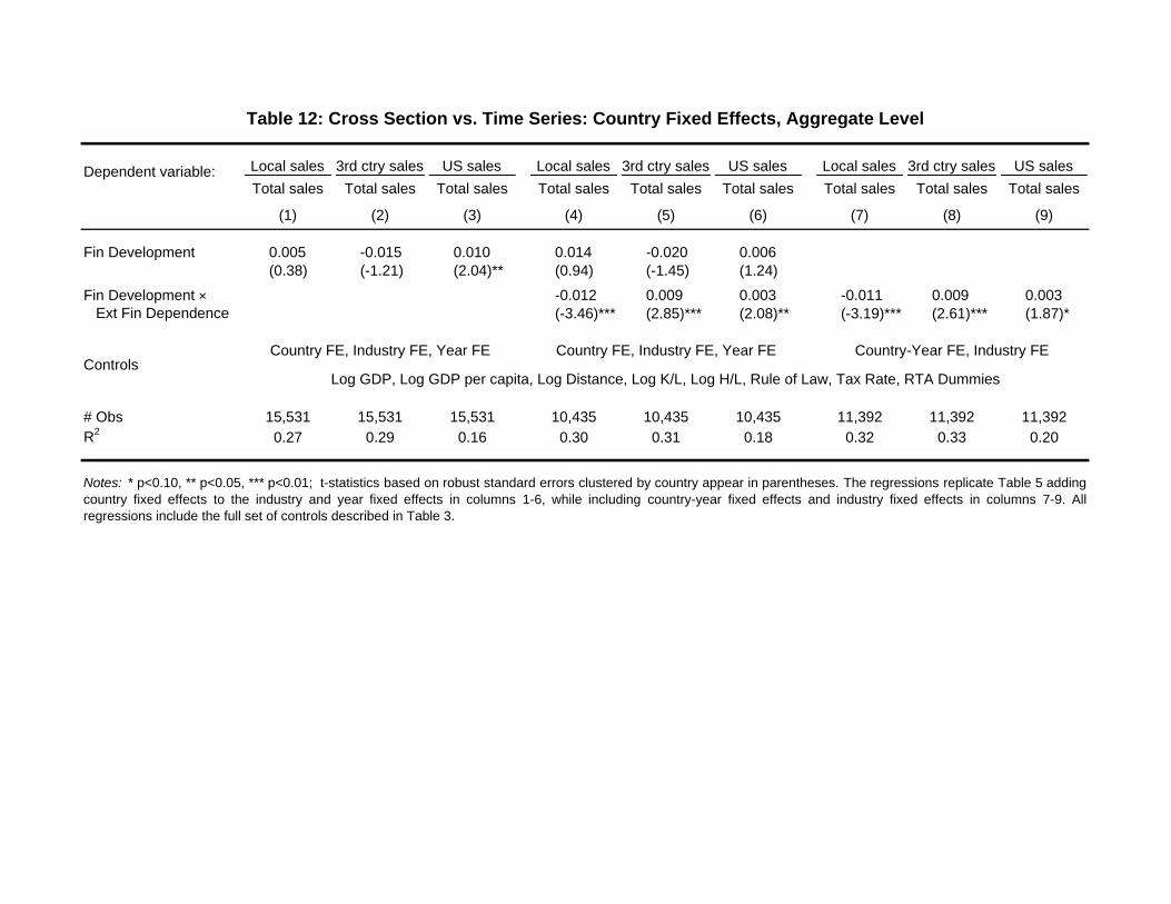
Local sales 3rd ctry sales US sales Local sales 3rd ctry sales US sales Local sales 3rd ctry sales US salesTotal sales Total sales Total sales Total sales Total sales Total sales Total sales Total sales Total sales

(1) (2) (3) (4) (5) (6) (7) (8) (9)

Fin Development 0.005 -0.015 0.010 0.014 -0.020 0.006(0.38) (-1.21) (2.04)** (0.94) (-1.45) (1.24)

Fin Development × -0.012 0.009 0.003 -0.011 0.009 0.003 Ext Fin Dependence (-3.46)*** (2.85)*** (2.08)** (-3.19)*** (2.61)*** (1.87)*

# Obs 15,531 15,531 15,531 10,435 10,435 10,435 11,392 11,392 11,392R2 0.27 0.29 0.16 0.30 0.31 0.18 0.32 0.33 0.20

Table 12: Cross Section vs. Time Series: Country Fixed Effects, Aggregate Level

Dependent variable:

Log GDP, Log GDP per capita, Log Distance, Log K/L, Log H/L, Rule of Law, Tax Rate, RTA Dummies

Notes: * p<0.10, ** p<0.05, *** p<0.01; t-statistics based on robust standard errors clustered by country appear in parentheses. The regressions replicate Table 5 addingcountry fixed effects to the industry and year fixed effects in columns 1-6, while including country-year fixed effects and industry fixed effects in columns 7-9. Allregressions include the full set of controls described in Table 3.

Country-Year FE, Industry FECountry FE, Industry FE, Year FE Country FE, Industry FE, Year FEControls

Dependent variable: GDP per capita growth

Time horizon:

(1) (2) (3) (4)

Aggregate MNC Sales Growth 0.165*** 0.189*** 0.107*** 0.137***(0.0322) (0.0283) (0.0295) (0.0202)

Growth in Share Local MNC Sales 0.618* 0.193**(0.324) (0.0820)

Growth in Share US MNC Sales 0.479 -0.131(0.349) (0.0865)

Initial log GDP per capita -0.053 -0.0576 -0.015* -0.020**(0.0374) (0.0385) (0.00783) (0.00895)

# Obs 44 38 204 164R2 0.549 0.593 0.199 0.325

Appendix Table 1: Economic Growth and Multinational Activity

Notes: * p<0.10, ** p<0.05, *** p<0.01; t-statistics based on robust standard errors in Columns 1-2 andclustered by country in Columns 3-4 appear in parentheses. The unit of observation is the country in columns1-2 and the country-period in columns 3-4, where a period is a 5-year interval between benchmark years in1989-2009. The dependent variable is the cumulative growth in GDP per capita over the period indicated inthe row heading. The right-hand side variables are cumulative growth rates in aggregate MNC sales or in thecomposition of aggregate MNC sales over the concurrent period.

1989-2009 5-Year Periods in 1989-2009

Country Mean St Dev Country Mean St Dev Country Mean St Dev

Algeria 0.15 0.16 Guatemala 0.21 0.08 Peru 0.17 0.08Argentina 0.16 0.05 Guyana 0.43 0.08 Philippines 0.29 0.10Australia 0.82 0.23 Haiti 0.13 0.02 Poland 0.25 0.09Austria 0.99 0.10 Honduras 0.35 0.10 Portugal 1.05 0.45Bahrain 0.41 0.07 Hong Kong 1.43 0.14 Qatar 0.29 0.04Bangladesh 0.28 0.06 Hungary 0.38 0.14 Russia 0.19 0.12Belgium 0.71 0.18 Iceland 0.88 0.76 Saudi Arabia 0.26 0.07Bolivia 0.41 0.13 India 0.30 0.09 Senegal 0.20 0.04Botswana 0.14 0.04 Indonesia 0.33 0.13 Singapore 0.92 0.12Brazil 0.35 0.08 Iran 0.21 0.04 Slovakia 0.41 0.07Bulgaria 0.34 0.22 Ireland 1.01 0.59 Slovenia 0.44 0.22Cameroon 0.12 0.07 Israel 0.71 0.14 South Africa 0.63 0.10Canada 0.96 0.24 Italy 0.71 0.18 Spain 1.05 0.42Chile 0.55 0.12 Jamaica 0.22 0.05 Sri Lanka 0.23 0.08Colombia 0.30 0.07 Japan 1.49 0.41 Sudan 0.04 0.02Congo 0.06 0.05 Jordan 0.71 0.12 Sweden 0.69 0.35Costa Rica 0.22 0.12 Kenya 0.22 0.02 Switzerland 1.61 0.07Cote D'Ivoire 0.20 0.09 Kuwait 0.47 0.19 Syria 0.09 0.01Croatia 0.61 0.13 Luxembourg 1.24 0.47 Tanzania 0.09 0.05Cyprus 1.42 0.36 Malawi 0.07 0.02 Thailand 1.03 0.28Czech Republic 0.49 0.14 Malaysia 1.09 0.22 Trinidad & Tobago 0.30 0.03Denmark 0.97 0.70 Malta 0.97 0.15 Tunisia 0.54 0.04Dominican Rep 0.21 0.05 Mexico 0.19 0.06 Turkey 0.17 0.07Ecuador 0.23 0.06 Morocco 0.43 0.17 Uganda 0.05 0.02Egypt 0.38 0.12 Netherlands 1.24 0.43 United Kingdom 1.31 0.30El Salvador 0.35 0.09 New Zealand 1.05 0.25 Uruguay 0.32 0.15Finland 0.69 0.14 Norway 0.64 0.09 Venezuela 0.13 0.07France 0.91 0.09 Oman 0.34 0.04 Vietnam 0.51 0.28Gabon 0.11 0.04 Pakistan 0.24 0.02 Yemen 0.06 0.01Germany 1.05 0.10 Panama 0.69 0.18 Zambia 0.07 0.03Ghana 0.08 0.04 Papua New Guinea 0.18 0.05Greece 0.50 0.24 Paraguay 0.22 0.05

Panel Variation: 0.51 0.44

Notes: This table summarizes the variation in financial development in the panel, as measured by private credit normalizedby GDP. Lebanon is further included in our sample in Table 8, Panel B, where financial development is measured insteadby stock market capitalization normalized by GDP.

Appendix Table 2: Host-Country Financial Development

Local sales 3rd ctry sales US sales Local sales 3rd ctry sales US salesTotal sales Total sales Total sales Total sales Total sales Total sales

(1) (2) (3) (4) (5) (6)

Fin Development -0.058 0.057 0.060 -0.060 0.055 0.052(-2.88)*** (2.15)** (3.42)*** (-2.92)*** (2.11)** (3.37)***

Fin Development × -0.013 0.008 0.007 Ext Fin Dependence (-3.71)*** (2.13)** (2.95)***

Controls

# observations 15,531 15,531 15,531 10,435 10,435 10,435R-squared 0.37 0.30 0.27 0.42 0.31 0.38

Local sales 3rd ctry sales US sales Local sales 3rd ctry sales US salesTotal sales Total sales Total sales Total sales Total sales Total sales

(1) (2) (3) (4) (5) (6)

Fin Development -0.051 0.032 0.019 -0.046 0.034 0.012(-2.56)** (1.89)* (2.40)** (-2.10)** (1.80)* (1.34)

Fin Development × -0.008 0.004 0.004 Ext Fin Dependence (-3.86)*** (2.39)** (2.06)**

Controls

# observations 210,852 210,852 210,852 159,137 159,137 159,137R-squared 0.16 0.18 0.09 0.16 0.18 0.11

Dependent variable:

Dependent variable:

Appendix Table 3: Tobit, Aggregate Level

Log GDP, Log GDP per capita, Log Distance, Log K/L, Log H/L, Rule of Law, Tax Rate, RTA Dummies, Industry FE, Year FE

Log GDP, Log GDP per capita, Log Distance, Log K/L, Log H/L, Rule of Law, Tax Rate, RTA Dummies, Industry FE, Year FE

Notes: * p<0.10, ** p<0.05, *** p<0.01; t-statistics based on robust standard errors clustered by country appear inparentheses. The regressions replicate Table 5, but apply Weighted Least Squares instead of OLS estimation, using log totalaffiliate sales as weights. All regressions include the full set of controls described in Table 3, as well as industry and year fixedeffects.

Notes: * p<0.10, ** p<0.05, *** p<0.01; t-statistics based on robust standard errors clustered by country appear inparentheses. The regressions replicate Table 5, but apply Tobit instead of OLS estimation. All regressions include the full setof controls described in Table 3, as well as industry and year fixed effects.

Appendix Table 4: Weighted Least Squares, Affiliate Level

Local sales 3rd ctry sales US sales Local sales 3rd ctry sales US salesTotal sales Total sales Total sales Total sales Total sales Total sales

(1) (2) (3) (4) (5) (6)

Fin Development 0.782 -0.702 -0.080 0.088 -0.079 -0.009(2.31)** (-2.41)** (-0.67) (0.65) (-0.73) (-0.17)

Fin Development × -0.013 0.010 0.003 -0.013 0.010 0.003 Ext Fin Dependence (-3.72)*** (3.07)*** (2.29)** (-3.70)*** (3.05)*** (2.29)**Fin Development × -0.071 0.062 0.009 Industry Capital Intensity (-2.47)** (2.51)** (0.87)Fin Development × -0.140 0.111 0.029 Industry Skill Intensity (-1.12) (1.10) (0.59)

Controls

# Obs 10,435 10,435 10,435 10,435 10,435 10,435R2 0.24 0.25 0.15 0.24 0.25 0.15

Dependent variable:

Notes: * p<0.10, ** p<0.05, *** p<0.01; t-statistics based on robust standard errors clustered by country appear in parentheses.The regressions replicate columns 4-6 of Table 5 adding: financial development interacted with industry capital intensity, andfinancial development interacted with industry skill intensity. The measures of capital and skill intensity are computed from theNBER CES Manufacturing Dataset, as the log real capital stock divided by total employment, and log nonproduction workersdivided by total employment respectively. All regressions include the full set of controls described in Table 3, as well as industryand year fixed effects.

Appendix Table 5: Interacting Financial Development with

Log GDP, Log GDP per capita, Log Distance, Log K/L, Log H/L, Rule of Law, Tax Rate, RTA Dummies, Industry FE, Year FE

Other Industry Variables, Aggregate Level

Local sales 3rd ctry sales US sales Local sales 3rd ctry sales US sales Local sales 3rd ctry sales US salesTotal sales Total sales Total sales Total sales Total sales Total sales Total sales Total sales Total sales

(1) (2) (3) (4) (5) (6) (7) (8) (9)

Fin Development -0.066 0.020 0.045 -0.048 0.033 0.015 -0.025 0.025 -0.000(-0.96) (0.39) (1.26) (-1.96)* (1.57) (1.24) (-0.97) (1.46) (-0.02)

Fin Development × -0.007 0.003 0.004 -0.007 0.002 0.004 -0.007 0.003 0.003 Ext Fin Dependence (-3.21)*** (1.87)* (1.90)* (-2.86)*** (1.77)* (1.99)** (-3.22)*** (1.81)* (1.84)*Log Parent Sales 0.012 -0.011 -0.000

(2.26)** (-3.07)*** (-0.13)Fin Development × 0.001 0.001 -0.002 Log Parent Sales (0.26) (0.30) (-0.83)Parent R&D / Sales -0.017 -0.038 0.055

(-0.24) (-0.62) (2.41)**Fin Development × -0.019 0.057 -0.038 Parent R&D / Sales (-0.27) (1.01) (-1.82)**Affiliate Wage 0.000 -0.000 -0.000

(1.57) (-1.23) (-1.23)Fin Development × -0.000 0.000 0.000 Affiliate Wage (-1.62) (1.19) (1.33)

Controls

# Obs 120,447 120,447 120,447 120,448 120,448 120,448 149,089 149,089 149,089R2 0.15 0.17 0.10 0.15 0.17 0.10 0.16 0.18 0.12

Dependent variable:

Log GDP, Log GDP per capita, Log Distance, Log K/L, Log H/L, Rule of Law, Tax Rate, RTA Dummies, Industry FE, Year FE

Appendix Table 6: Interacting Financial Development with Other Firm Variables, Affiliate Level

Notes: * p<0.10, ** p<0.05, *** p<0.01; t-statistics based on robust standard errors clustered by country appear in parentheses. The regressions replicate columns 4-6 of Table 7adding: financial development interacted with log parent sales, financial development interacted with parent R&D divided by sales, and financial development interacted with theaffiliate average wage compensation per worker. All firm-level variables are calculated from the Bureau of Economic Analysis Survey of U.S. Direct Investment Abroad. Allregressions include the full set of controls described in Table 3, as well as industry and year fixed effects.

Local sales 3rd ctry sales US sales Local sales 3rd ctry sales US salesTotal sales Total sales Total sales Total sales Total sales Total sales

(1) (2) (3) (4) (5) (6)

Panel A: EU host countries

Fin Development 0.006 -0.014 0.008 0.013 -0.018 0.005(0.21) (-0.54) (1.40) (0.45) (-0.61) (0.83)

Fin Development × -0.015 0.012 0.003 Ext Fin Dependence (-2.92)*** (2.18)** (1.52)

Controls

# Obs 6,098 6,098 6,098 4,191 4,191 4,191R2 0.32 0.30 0.14 0.31 0.29 0.11

Panel B: Non-EU host countries

Fin Development -0.097 0.066 0.030 -0.098 0.071 0.027(-3.53)*** (2.60)** (3.68)*** (-3.58)*** (2.65)*** (3.63)***

Fin Development × -0.009 0.007 0.002 Ext Fin Dependence (-2.14)** (1.87)* (1.11)

Controls

# Obs 9,433 9,433 9,433 6,244 6,244 6,244R2 0.22 0.21 0.16 0.16 0.22 0.19

Appendix Table 7: EU vs non-EU Host Countries, Aggregate Level

Dependent variable:

Log GDP, Log GDP per capita, Log Distance, Log K/L, Log H/L, Rule of Law, Tax Rate, RTA Dummies, Industry FE, Year FE

Notes: * p<0.10, ** p<0.05, *** p<0.01; t-statistics based on robust standard errors clustered by country appear inparentheses. The regressions replicate columns 4-6 of Table 5 for the EU and non-EU host country sub-samples respectively.All regressions include the full set of controls described in Table 3, as well as industry and year fixed effects.

Log GDP, Log GDP per capita, Log Distance, Log K/L, Log H/L, Rule of Law, Tax Rate, RTA Dummies, Industry FE, Year FE

Notes: This figure summarizes the breakdown of multinational firms' affiliate activity by market destination in 1989. Affiliates in the red circleare engaged in horizontal sales; in the blue circle - in return sales to the US; and in the yellow circle - in export-platform sales to third-countries. Affiliates in overlapping segments of the three circles pursue multiple sales destinations. The percentages reported sum to 100%.Each segment reports the percentage share of affiliates active in a given set of destinations (Figure 1a) or the percentage share of totalaffiliate sales captured by affiliates in that segment (Figure 1b).

Figure 1a

The Distribution of MNC Affiliate Sales across Destinations

The Distribution of MNC Affiliates by Active Sales Destinations

Figure 1b

Return Sales

21.6%

44.3%

2.0% 3.0%

5.6% 21.6%

1.7%

Horizontal Sales

Platform Sales

Return Sales

52.3%

19.8%

0.6% 1.7%

6.0% 17.5%

2.1%

Horizontal Sales

Platform Sales

Figure 2: An ExampleMNC Sales Shares in Host Countries at Different Levels of Financial Development

Brazil, 1999 Chile, 1994 Norway, 1989Fin Devt: 0.29 Fin Devt: 0.43 Fin Devt: 0.61

MNC Sales/GDP: 0.042 MNC Sales/GDP: 0.048 MNC Sales/GDP: 0.057

Notes: This figure illustrates how the level and composition of aggregate MNC affiliate sales vary across three host countriesat the 50th, 60th and 75th percentiles of the distribution of financial development. Financial Development is measured by theratio of private credit to GDP.

0

0.1

0.2

0.3

0.4

0.5

0.6

0.7

0.8

0.9

Local MNC Sales US MNC Sales 3rd Country MNC Sales

Appendix Figure 1: Economic Growth and Multinational Activity, 1989-2009

Figure 1a: Growth in Total MNC Sales Figure 1b: Growth in the Share of Local MNC Sales

Notes: This figure illustrates the relationship between economic growth and growth in aggregate multinational activity from 1989 to 2009 across 44 host countries.Observations are labeled by their country ISO code. Plotted on the vertical axis of each figure is the cumulative growth in GDP per capita. Plotted on the horizontal axis isthe cumulative growth in aggregate MNC sales (Figure 1a), as well as the cumulative growth in the shares of aggregate MNC sales sold in the host-country market(Figure 1b), in the US (Figure 1c), and in third-country markets (Figure 1d).

Figure 1c: Growth in the Share of US MNC Sales Figure 1d: Growth in the Share of 3-rd Country MNC Sales

ARE

ARG

AUS

AUTBELBMU

BRA

BRB

CAN

CHE

CHL

COL

DEU DNK

DOM

ECU

ESP

FINFRA

GBR

GRC

HKG

IDN

IND

IRL

ISR

ITAJPN

KOR

LUX

MEX

NLDNOR

NZL

PAN

PHLPRT

SGP

SWE

TUR

TWN

VEN

ZAF

-.50

.51

1 2 3 4 5Total MNC sales growth 1989-2009

GDP per capita growth from 1989-2009 Fitted values

ARE

ARG

AUS

AUT BELBMU

BRA

BRB

CAN

CHE

CHL

COL

DEUDNK

DOM

ECU

ESP

FINFRA

GBR

GRC

HKG

IDN

IRL

ITAJPN

KOR

LUX

MEX

NLDNOR

NZL

PAN

PHL PRT

SGP

SWE

TUR

TWN

VEN

ZAF

-.50

.51

-.4 -.2 0 .2 .4 .6Growth in fraction local sales 1989-2009

GDP per capita growth from 1989-2009 Fitted linear line

ARE

ARG

AUS

AUTBELBMU

BRA

BRB

CAN

CHE

CHL

COL

DEUDNK

DOM

ECU

ESP

FRA

GBR

GRC

HKG

IDN

IRL

ISR

ITAJPN

KOR

MEX

NLDNOR

NZL

PAN

PHL

SGP

TUR

TWN

VEN

ZAF

-.50

.51

-.6 -.4 -.2 0 .2Growth in fraction US sales 1989-2009

GDP per capita growth from 1989-2009 Fitted linear line

ARE

ARG

AUS

AUTBELBMU

BRA

BRB

CAN

CHE

CHL

COL

DEU DNK

DOM

ECU

ESP

FRA

GBR

GRC

HKG

IDN

IND

IRL

ITAJPN

KOR

MEX

NLDNOR

NZL

PAN

PHL

SGP

TUR

TWN

VEN

ZAF

-.50

.51

-.2 0 .2 .4 .6Growth in fraction third-country sales 1989-2009

GDP per capita growth from 1989-2009 Fitted linear line

Host-Country Financial Development and Multinational Activity:

Model Appendix

L. Kamran Bilir∗

University of Wisconsin – Madison

Davin Chor

National University of Singapore

Kalina Manova

University of Oxford,

NBER and CEPR

October 15, 2016

Abstract

This Model Appendix develops a three-country model with heterogeneous firms, to formally demonstrate

the competition effect and the financing effect of host-country financial development. The predictions of the

model for various dimensions of multinational activity are derived, both at the level of the individual affiliate,

as well as at the aggregate level (i.e., summing across all affiliates in the host country). Several extensions

to more general modeling setups are discussed; these incorporate: (i) home-bias in consumption; (ii) exports

of host-country varieties; (iii) endogenous host-country wages; and (iv) multiple FDI host countries.

A Model Appendix: Preamble

In this Model Appendix, we develop in full a three-country model with heterogeneous firms to analyze how

host-country financial development affects the entry and sales decisions of multinational affiliates. The model

is in the spirit of Helpman, Melitz and Yeaple (2004) and Grossman, Helpman and Szeidl (2006): Firms obtain

a productivity draw, and subsequently sort themselves into different production modes (i.e., exports vs FDI)

for servicing each country market. We introduce into this setup financial frictions in the country that is the

potential FDI host, and then derive how improvements in host-country financial development would impact a

series of outcome variables related to affiliate entry and sales.

The model is relatively stylized, given that its purpose is to demonstrate in a parsimonious setting how the

competition and financing effects operate, and to show how these theoretical results then motivate the empirical

analysis conducted in the main paper. We describe the baseline three-country setup in Section A.1 below, this

being the simplest setting in which the concepts of local affiliate sales, return sales to the home country, and

third-country platform sales are well-defined. Only domestic firms in the FDI host country rely on host-country

financial institutions in this baseline, a setting which will isolate the competition effect from improvements in

host-country financial development (Section A.2). We then incorporate host-country borrowing on the part of

multinational affiliates, to demonstrate the richer predictions that this financing effect leads to (Section A.3).

∗L. Kamran Bilir: University of Wisconsin – Madison, [email protected]. Davin Chor: National University of Singapore,[email protected]. Kalina Manova (corresponding author): Department of Economics, University of Oxford, Manor RoadBuilding, Manor Road, OX1 3UQ, UK, [email protected].

1

Several extensions are also discussed, related to incorporating: (i) home-bias in consumption (Section A.4.1);

(ii) exports of host-country varieties (Section A.4.2); (iii) endogenous host-country wages (Section A.4.3); and

(iv) multiple FDI host countries (Section A.4.4). These extensions serve to illustrate how the two key effects

of host-country financial development extend to more general modeling setups. Last but not least, Section A.5

discusses how the predictions of the model translate into the empirical specification that we adopt in the main

paper. Detailed algebraic derivations are in the final section of this Appendix (Section B).

A.1 Baseline Model Setup

Consider a world with three countries, West, East, and South. There are two sectors in each country, one

producing a homogeneous good and the other featuring a continuum of differentiated varieties. Labor is the

only factor of production. The homogeneous good is manufactured under constant returns to scale. This good

is freely tradable across borders, and thus serves as the global numeraire. In each country, the labor force is

sufficiently large so that a strictly positive amount of the homogeneous good is produced in equilibrium. We

assume for simplicity that West and East are symmetric in their underlying economic structure. However,

South is less productive in the homogeneous good sector than West and East: While 1/ω workers are needed

to make each unit of the numeraire in South (where ω < 1), only one worker is required in West and East.

The nominal wage in West and East is thus 1, while the wage in South is ω. Firms manufacturing in South

therefore face lower production costs.1

The utility function of a representative consumer in West and East (subscript n = w, e) is given by:

Un = y1−µn

∑j∈e,w

∫Ωnj

xnj(a)α dGj(a)

µα

, (A.1)

while the utility function for Southern consumers (subscript s) is:

Us = y1−µs

∑j∈e,w,s

∫Ωsj

xsj(a)α dGj(a)

µα

, 0 < α, µ < 1. (A.2)

Utility in country i (i ∈ w, e, s) is thus a Cobb-Douglas aggregate over consumption of the homogeneous

good (yi) and differentiated varieties (xij(a)), where the expenditure share of the latter is equal to µ. The sub-

utility derived from differentiated varieties is a Dixit-Stiglitz aggregate with a constant elasticity of substitution

ε = 11−α > 1.2

Let xij(a) denote the quantity of a country-j differentiated variety that is consumed in country i, and label

the set of such varieties Ωij . When i 6= j, this set consists of all varieties exported by country j’s firms to i, as

well as any varieties produced and sold locally by country j’s multinational affiliates in i. Analogously, when

i = j, Ωii represents all indigenous varieties produced domestically, and all varieties produced by country i’s

multinational affiliates abroad that are then exported back to the home market. Notice that South demands

varieties from all three countries, while Southern varieties do not enter the utility function of West and East.

This assumption simplifies our analysis but does not detract from our main results (see Section A.4.2, which

1In principle, many factors influence the relative profitability of manufacturing across locations, including not only factor prices,but also institutions, trade costs, and coordination costs. We focus on a model with wage differences for simplicity, and assume thatthese differences are exogenous as a baseline. We have evaluated numerically a more general setting in which the homogeneous goodsector is absent and ω therefore adjusts endogenously, in order to verify the extent to which the competition effect we emphasizeremains active even when Southern wages adjust; see Appendix A.4.3.

2For now, this elasticity is the same regardless of varieties’ country of origin, but we discuss in Section A.4.1 a more flexiblespecification in which varieties from the same country are closer substitutes than varieties from different countries.

2

features exports of Southern varieties to West and East).

Consumer preferences (A.1) and (A.2) imply that demand in country i for each country-j variety is xij(a) =

Aijpij(a)−ε, where pij(a) denotes the price of that variety in i. Given the symmetric economic structures of

West and East, the aggregate demand levels, Aij , in country i for varieties from j are:

Aww = Aee = Aew = Awe =µEn

P 1−εww + P 1−ε

we

, and (A.3)

Asw = Ase = Ass =µEs

P 1−εss + 2P 1−ε

sw

, (A.4)

where P 1−εij =

∫Ωij

pij(a)1−εdGj(a) is the ideal price index for country-j varieties in i. Note in particular

that P 1−εww = P 1−ε

ee , P 1−εew = P 1−ε

we and P 1−εsw = P 1−ε

se , given the underlying assumption of symmetry between

West and East. In the above, Ei denotes the total expenditure of consumers in i and Ew = Ee = En. These

expenditure levels are exogenous and equal to aggregate labor income in each country.

We proceed next to describe the structure of production in each country’s differentiated varieties sector.

There is a continuum of firms in each country that can engage in the production of differentiated varieties.

Upon paying a fixed entry cost, each such firm in country j draws a unit labor requirement a for producing its

distinct variety from a distribution Gj(a) that represents the technological possibilities in j. The productivity

level of firm a is therefore 1/a.

A.1.1 Financially unconstrained firms in West and East

Consider the differentiated varieties sector in West; conditions are symmetric in East.3 After observing its unit

cost draw a, each entrant in West decides whether to commence production or exit. Should the firm choose to

remain active, production for the home economy incurs a per-period fixed cost of fD units of Western labor.

One can interpret this as the recurring cost of operating a manufacturing plant in West. Firms need to pay fD

upfront at the beginning of each period, but they cannot use retained earnings from previous periods because

management has no control rights over these revenues and must transfer them as dividends or profits to the

firm’s owners. Firms therefore raise external finance by borrowing at a (gross) interest rate of R > 1, which

is set exogenously in an international capital market. However, there are no financial frictions and hence no

credit rationing in West and East.

Firms charge a constant markup over marginal costs, with the home price for a Western variety being

pww(a) = aα . Individual producers take the aggregate demand levels in each country as given. Profits from

domestic sales in West thus equal:

πD(a) = (1− α)Aww

( aα

)1−ε−RfD. (A.5)

The export decision: Western firms may export to East or South (or both). Exporting to a foreign

market incurs a per-period fixed cost of fX units of Western labor (for maintaining an overseas distribution

network) and a variable iceberg transport cost, τ > 1. Profits from exporting to East and South are thus

respectively:

πXN (a) = (1− α)Aew

(τaα

)1−ε−RfX , and (A.6)

πXS(a) = (1− α)Asw

(τaα

)1−ε−RfX . (A.7)

3The corresponding equations for East can be obtained by replacing the subscript ‘w’ with ‘e’, and vice versa.

3

The FDI decision: Western firms may also choose to become multinationals by locating production

abroad. A multinational firm would save on shipping costs on its sales in the host-country market, and would

moreover lower its wage bill if it locates an affiliate in South. Such a firm could use its foreign subsidiary not

only to supply the host economy, but also to export back to its parent country (West) or to the third-country

market (East); we refer to these as local, return and platform sales, respectively. Should the affiliate export

to either East or West, this would incur fixed and variable trade costs, fX and τ (as in “The export decision”

above), for each destination market.

Establishing a foreign subsidiary requires an upfront per-period fixed cost of fI units of Western labor, in

order to set up and maintain production facilities, as well as to manage operations remotely. While financial

conditions are identical in West and East, there are financial frictions in South and the implied cost of capital

there (weakly) exceeds R, in the sense that not all firms that seek financing in South will successfully obtain it.

A multinational company thus has no incentive to raise capital abroad as long as Western financiers are willing

to fully fund fI . (This assumption will be relaxed in Section A.3 when we introduce the financing effect.)

A Western multinational faces in principle a wide array of options for its export-versus-FDI decision over

the three markets. For this reason, multi-country models of FDI with export platforms are analytically complex

(Yeaple 2003a,b, 2013, Tintelnot 2016). To illustrate the competition effect as transparently as possible, we

therefore focus here on the case where: (i) Western multinationals locate affiliates only in South; and (ii)

Western multinationals use the Southern plant as a global production center to serve all three markets. For

this case, we derive testable implications with a clear mapping between theoretical expressions and observable

data. We show in the detailed derivations in Section B.1 that two conditions on parameters guarantee that the

FDI pattern we consider is indeed the optimal strategy for Western multinationals: τω < 1 and fX < fD < fI .

Intuitively, the fixed export cost (fX) and the Southern wage after adjusting for transport costs (τω) must both

be low for MNCs to optimally use South as their global production center.

Under these parameter assumptions, and taking into account revenues from all three markets, profits from

FDI in South for a firm with productivity 1/a are therefore:

πI(a) = (1− α)Asw

(aωα

)1−ε+ (1− α)(Aww +Aew)

(τaωα

)1−ε−R(fI + 2fX). (A.8)

Patterns of production: Each firm’s productivity level determines where it manufactures and in which

markets it sells its goods. Firms produce at home for the domestic market if profits from (A.5) are positive.

Solving πD(a) = 0 pins down aD, the maximum labor input requirement at which domestic production is

profitable. Similarly, setting πXN (a) = 0 yields a cutoff level, aXN , below which exporting to East is profitable.

Solving πXS(a) = 0 delivers the analogous cutoff, aXS , for exporting to South. The expression for these three

thresholds are:

a1−εD =

RfD(1− α)Aww(1/α)1−ε , (A.9)

a1−εXN =

RfX(1− α)Aew(τ/α)1−ε , and (A.10)

a1−εXS =

RfX(1− α)Asw(τ/α)1−ε . (A.11)

A fourth cutoff, aI , delineates when FDI is feasible. Becoming a multinational is more profitable than basing

production in West when πI(a) > πD(a) + πXN (a) + πXS(a). Solving this as an equality delivers the following

expression for aI :

4

a1−εI =R(fI − fD)

(1− α)[Aww(( τωα

)1−ε − ( 1α

)1−ε) +Aew(( τωα

)1−ε − ( τα

)1−ε) +Asw((ωα

)1−ε − ( τα

)1−ε)]. (A.12)

Note that the conditions fI > fD, τω < 1, ω < 1 < τ and ε > 1 ensure that aI > 0.

Following common practice in the literature, we consider industry equilibria in which 0 < a1−εD < a1−ε

XN <

a1−εXS < a1−ε

I , using a1−ε as a proxy for firm productivity. This describes a sorting of Western firms across

production modes that is in line with prior evidence that exporting firms tend to be more productive than

non-exporters, while multinationals are on average more productive than exporters (e.g., Helpman et al. 2004).

The least efficient firms with a1−ε < a1−εD have labor input requirements that are too high and exit the

industry upon observing their productivity draw. Firms with productivity levels between a1−εD and a1−ε

XN supply

only the domestic Western market. Using (A.9) and (A.10), the assumption that a1−εD < a1−ε

XN reduces to

τε−1(fXAew

)> fD

Aww, so that export costs must be sufficiently bigger than the fixed cost of domestic production.4

Next, those firms that are even more productive, with a1−εXN < a1−ε < a1−ε

XS , are able to overcome the additional

costs of exporting to East, but not to South; based on (A.10) and (A.11), this simply requires that market

demand for Western varieties be greater in East than in South, Aew > Asw. Firms with a1−εXS < a1−ε < a1−ε

I can

further export to the smaller Southern market.5 Finally, the most productive firms with a1−ε > a1−εI conduct

FDI in South. Figure A.1 provides an illustration of this industry structure that focuses on the economic

relations in our three-country world. Firms with a1−ε < a1−εI base their production activity in West, and

export to East and possibly also to South if they are productive enough (upper panel). On the other hand,

the most efficient firms with a1−ε > a1−εI become multinationals. While these firms are still headquartered in

West, their production is located in South, from where they service all three markets (lower panel).

A.1.2 Credit-constrained firms in South

The structure of South’s differentiated varieties sector is simpler, with Southern firms producing only for

domestic consumption in this baseline model. The fixed cost of domestic production is fS units of Southern

labor, and we assume as above that Southern firms borrow at the start of each period to finance these fixed

costs.

However, Southern firms face credit constraints, arising from institutional weaknesses that lead to imperfect

protection for lenders against default risk. Following Aghion et al. (2005), we model this moral hazard problem

by assuming that firms lose a fraction η ∈ [0, 1] of their appropriable profits if they choose to default. For

simplicity, we take these appropriable profits to be the revenues of the firm less the variable costs that it must

pay to its production workers. Thus, while it is tempting to default to avoid loan repayment, the act of hiding

the firm’s financial resources from lenders incurs a pecuniary cost that is increasing in the parameter η. We

therefore interpret η as capturing the degree of financial development in South: When credit institutions are

stronger, η is higher and it is more costly for firms to opt for default. A Southern firm with input coefficient a

would default if and only if the associated profit loss is smaller than the cost of repaying the loan:

η(1− α)Ass

(aωα

)1−ε< RfSω.

The above condition yields a productivity threshold above which firms have access to credit:

a1−εS =

1

η

RfSω

(1− α)Ass(ω/α)1−ε . (A.13)

4Under the utility specification in (A.1) and (A.2) with a single elasticity of substitution, we have Aww = Aew, so this conditionsimplifies further to τε−1fX > fD. Note that this is not inconsistent with the earlier requirement that fX < fD.

5The parameter restriction that guarantees that a1−εXS < a1−εI does not simplify neatly. Intuitively, it requires that the fixedcost of FDI, fI , be sufficiently large so that FDI is only undertaken by the most productive firms.

5

Figure 1 Modes of Operation (illustrated for Western firms)

If a1-aI

1-No FDI):

If a1-aI 1-FDI in South):

West

South

East

Return exports to West: RET(a)

Platform exports to East: PLA(a)

Local market sales: HOR(a)

West

South

East

Export to East if:

aXN 1-< a1-

Export to South if:

aXS1-< a1-

Produce for Home if:

aD 1-a1-

Figure 1: Modes of Operation (illustrated for Western firms)

6

We assume that lenders can observe a, and hence only Southern firms with a1−ε > a1−εS are able to commence

production. When η = 1, a1−εS is the cutoff for domestic entry that would prevail in the absence of credit

market imperfections. When η < 1, however, the cutoff is higher, as some firms with productivity below a1−εS

would earn positive profits following entry, but are prevented from doing so because they are unable to credibly

commit to repaying their loans. As η increases toward 1, this distortion from credit constraints vanishes.

A.1.3 Industry equilibrium

The model is closed by specifying the conditions that govern firm entry in each country. Prospective entrants

in country i’s differentiated varieties sector incur an upfront entry cost equal to fEi units of country i labor.

This is a once-off cost that firms pay before they can obtain their productivity draw.6 On the exit side, firms

face an exogenous probability, δ ∈ (0, 1), of “dying” and leaving the industry in each period. For an equilibrium

with a constant measure of firms in each country, the cost of entry must equal expected profits. Using the

profit functions (A.5)-(A.8) and the cutoffs (A.9)-(A.12), and integrating the expressions for expected profits

over the distribution Gi(a), one can write down the free-entry conditions for Western/Eastern (n = w, e) and

Southern firms as:

δfEn = (1− α)Aww

(1

α

)1−ε

(Vn(aD)− Vn(aI))−RfD(Gn(aD)−Gn(aI)) (A.14)

+(1− α)Aew( τα

)1−ε(Vn(aXN )− Vn(aI))−RfX(Gn(aXN )−Gn(aI))

+(1− α)Asw( τα

)1−ε(Vn(aXS)− Vn(aI))−RfX(Gn(aXS)−Gn(aI))

+(1− α)

(Aww

(τωα

)1−ε+Aew

(τωα

)1−ε+Asw

(ωα

)1−ε)Vn(aI)−R(fI + 2fX)Gn(aI), and

δfEsω = (1− α)Ass(ωα

)1−εVs(aS)−RfSωGs(aS). (A.15)

Note that Vi(a) is defined by Vi(a) =∫ a

0a1−εdGi(a) for i ∈ n, s.

Finally, we denote the measure of firms in country i’s differentiated varieties sector by Ni.7 The definition

of the ideal price index then implies:

P 1−εww = Nn

[(1

α

)1−ε

(Vn(aD)− Vn(aI)) +(τωα

)1−εVn(aI)

], (A.16)

P 1−εew = Nn

[( τα

)1−ε(Vn(aXN )− Vn(aI)) +

(τωα

)1−εVn(aI)

], (A.17)

P 1−εsw = Nn

[( τα

)1−ε(Vn(aXS)− Vn(aI)) +

(ωα

)1−εVn(aI)

], and (A.18)

P 1−εss = Ns

[(ωα

)1−εVs(aS)

]. (A.19)

The equilibrium of the model is thus pinned down by the system of equations (A.3)-(A.4) and (A.9)-(A.19)

in the 15 unknowns, Aww, Aew, Asw, Ass, aD, aXN , aXS , aI , aS , Nn, Ns, Pww, Pew, Psw and Pss. Although

not all of these variables can be solved for in closed form, comparative statics results can still be derived

that directly inform our empirical analysis. As is common in this literature, we assume that productivity 1/a

6Our results are robust to subjecting the fixed cost of entry in South, fEs, to borrowing constraints too. Intuitively, animprovement in financial development in South would still spur more entry by Southern firms, which works in the same directionas the effects in our baseline model.

7Following Melitz (2003), for Ni to be constant, the expected mass of successful entrants, Nenti , needs to equal the mass of

firms that dies exogenously in each period, namely: Nenti = δNi, for i = w, e, s.

7

follows a Pareto distribution with shape parameter k and support [1/ai,∞) for each country i.8 With this

distribution, the associated expressions for Gi and Vi are: Gi(a) =(aai

)kand Vi(a) = k

k−ε+1

(ak−ε+1

aki

). We

adopt the assumption that k > ε− 1, which ensures that the distribution of firm sales has a finite mean.

A.2 The Competition Effect

We can now derive how financing conditions in the host country affect various dimensions of multinational

activity, by establishing how an improvement in η systematically shifts the productivity cutoffs and aggregate

demand levels in each market. In the baseline where only Southern firms rely on host-country financial institu-

tions, we will see that an increase in η promotes entry by more Southern firms, which leads to the competition

effect vis-a-vis multinational affiliates.

A.2.1 Impact on industry cutoffs and market demand levels

Equations (A.13) and (A.15) pin down Ass and aS for the industry equilibrium in South. By totally differen-

tiating these two equations, we obtain:

Lemma 1: (i) daSdη > 0; and (ii) dAss

dη < 0.

We relegate all detailed proofs to Section B.1, and focus instead on conveying the intuition here. When η

rises, the higher cost of default in South helps to alleviate the moral hazard problem, and hence more Southern

firms gain access to credit. This lowers the productivity cutoff, a1−εS , for entry into the Southern differentiated

varieties sector, as illustrated in the bottom panel of Figure A.2. However, the free-entry condition (A.15)

requires that the expected profitability of a Southern firm remain constant. Average demand for each Southern

product, Ass, must subsequently fall.

Since Western, Eastern and Southern varieties are substitutes in consumption in South, the entry of more

domestic firms in South will affect the differentiated varieties sector in West and East. The consequent effects

on the productivity cutoffs and demand levels relevant to Western firms are described in the following lemma;

by symmetry, these comparative statics also apply to Eastern firms:

Lemma 2: When MNCs do not require host-country financing, (i) 1aXS

daXSdη < 1

aIdaIdη < 0; (ii) 1

aXNdaXNdη =

1aD

daDdη > 0; (iii) 1

AswdAswdη < 0; and (iv) 1

AewdAewdη = 1

AwwdAwwdη > 0.

The key shifts in Lemma 2 are illustrated in the upper panel of Figure A.2. An improvement in host-country

financial development leads to the entry of more Southern varieties, and the resulting tougher competition

decreases demand in South for each Western variety, Asw. This raises the productivity cutoffs, a1−εXS and a1−ε

I ,

for Western firms seeking to penetrate the Southern market either through exports or FDI. However, since the

fixed cost of entry, fEn, remains constant, the free-entry condition (A.14) implies that total profits from sales in

West and East must increase. This tilts Western firms toward serving those markets: The productivity cutoffs,

a1−εD and a1−ε

XN , both fall, while aggregate demand levels in West and East, Aww and Aew, both rise.9

8We require that as and an both be sufficiently large, so that all relevant cutoffs lie within the interior of the support of thedistributions that they are drawn from. Also, our proofs do not require the same shape parameter in West and South, but we haveassumed this to simplify notation.

9That the proportional shifts in Aww and Aew are equal is a feature that is relaxed in the extension in Section A.4.1.

8

Figure 2 Response of Cutoffs to an Improvement in Southern Financial Development:

Baseline Model

In West:

In South:

aS 1-

Firm Exits Production for South only

a1-

Cutoff for entry in South, in the absence of credit constraints

aD 1- aXN

1- aI 1-

Firm Exits

Production for Home only

Export to East

FDI in South

Export to East and South

aXS 1-

a1-

Figure 2: Response of Cutoffs to an Increase in η: Baseline Model

9

A.2.2 Impact on multinational affiliate sales

These shifts in the productivity cutoffs and aggregate demand levels in turn determine the impact of host-

country financial development on affiliate sales. We define several sales variables of interest that are observable

in the data, and which were also illustrated earlier in the lower panel of Figure A.1. For a given MNC affiliate

in South with productivity 1/a, its sales to the local market are: HOR(a) ≡ Asw(aωα

)1−ε. We refer to these as

horizontal sales, since they allow the multinational to avoid transport costs while servicing the Southern market.

Export-platform sales to third-country destinations (in our case, East) are defined as: PLA(a) ≡ Aew(τaωα

)1−ε.

Finally, return sales back to the Western home market are: RET (a) ≡ Aww(τaωα

)1−ε. The affiliate’s total sales

are: TOT (a) ≡ HOR(a) + PLA(a) +RET (a).

Integrating these firm-level sales over the set of Western multinationals (with a1−ε > a1−εI ) delivers the

following expressions for the aggregate levels of horizontal, platform and return sales (n = w, e):

HOR ≡ Nn

∫ aI

0

HOR(a)dGn(a) = NnAsw

(ωα

)1−εVn(aI), (A.20)

PLA ≡ Nn

∫ aI

0

PLA(a)dGn(a) = NnAew

(τωα

)1−εVn(aI), and (A.21)

RET ≡ Nn

∫ aI

0

RET (a)dGn(a) = NnAww

(τωα

)1−εVn(aI). (A.22)

The measure of multinational firms is in turn given by: Nn∫ aI

0dGn(a) = NnGn(aI).

Using these definitions, we construct three sales shares that describe the breakdown of affiliate sales by

destination:

HOR(a)

TOT (a)=HOR

TOT=

(1 + τ1−εAew

Asw+ τ1−εAww

Asw

)−1

, (A.23)

PLA(a)

TOT (a)=PLA

TOT=

(1 + τε−1Asw

Aew+AwwAew

)−1

, and (A.24)

RET (a)

TOT (a)=RET

TOT=

(1 + τε−1 Asw

Aww+AewAww

)−1

. (A.25)

Note that these sales shares depend crucially on the pairwise ratios of the aggregate demand levels for Western

varieties across the three different markets.

The following result states the effect of host-country financial development on each of the above measures

of multinational activity.10

Proposition 1 When MNCs do not require host-country financing, in response to a small improvement in

financial development, η, in South:

(i) HOR(a) decreases, while both PLA(a) and RET (a) increase;

(ii) HOR(a)TOT (a) = HOR

TOT decreases, while both PLA(a)TOT (a) = PLA

TOT and RET (a)TOT (a) = RET

TOT increase; and

(iii) Nn, NnGn(aI), HOR, PLA and RET all decrease.

Proposition 1 builds directly on the logic of Lemma 2. When credit constraints are eased, the demand

in South for Western goods drops due to the competition effect following the entry of more local firms. For

each affiliate, this leads horizontal sales to South, as well as their share in total sales, to decline. At the same

time, demand levels in East and West rise in equilibrium, so that each affiliate re-directs its sales toward those

10All results regarding affiliate-level sales pertain to firms that remain multinationals after the change in η.

10

markets. This prompts an increase in platform and return sales, both in absolute levels and relative to total

sales.

In the absence of other countervailing forces, the competition effect alone would reduce the ex ante expected

profits of Western firms. This leads to a decrease in both the measure of these firms, Nn, and the measure of

multinationals, NnGn(aI), as stated in part (iii) of the proposition. To see how this in turn affects aggregate

sales levels, we refer back to equations (A.20)-(A.22). On the extensive margin, a higher η lowers HOR, PLA

and RET , by reducing Nn and raising the productivity cutoff for FDI so that VN (aI) drops; both of these shifts

reflect the exit of Western MNCs from South. In the case of horizontal sales, this negative effect is reinforced

by the reduction in Asw, and HOR clearly falls. As for the platform and return sales, one can see that the

decline on the extensive margin can in principle be counteracted by the increase on the intensive margin in Aew

and Aww. In more general settings, this could lead to an ambiguous prediction for the effect of host-country

financial development on PLA, RET and hence TOT . In the context of our three-country model though, one

can explicitly prove that the decline on the extensive margin is the dominant effect; this three-country model

therefore provides an example of a setting in which PLA, RET and TOT do indeed all decrease in response to

a rise in η (see Section B.1).

As we will see below, this feature of a negative extensive margin adjustment in response to improvements

of host-country financial development can be relaxed by considering affiliate financing practices more closely.

We consider this issue next.

A.3 The Financing Effect

In our baseline setup, Western and Eastern firms are able to secure all the outside finance they need from

their home country. We now examine what happens when we consider multinationals that use some Southern

financing to cover their FDI costs, so that host-country financial development can now affect MNC activity not

only through the competition effect, but also through a direct financing channel. As argued in the main paper,

multinational affiliates are indeed commonly observed to obtain at least some financing from host-country

financing institutions (Desai et al. 2004, Feinberg and Phillips 2004). The literature has moreover reported

evidence that affiliate financing practices do indeed respond by shifting towards obtaining more host-country

financing when financial development in the FDI host improves (Desai et al. 2004, Antras et al. 2009).

These patterns suggest that while MNCs can use internal capital markets to some degree, there exist market

or institutional frictions that prevent them from doing so perfectly. First, fixed assets in a Southern plant might

not be fully collateralizable, due to expropriation risk or difficulties in enforcing cross-border claims. Second,

there might be asymmetric information between lenders and borrowers because lenders do not observe how

firms manage operations or customize production processes to local conditions. If creditors can more effectively

monitor debtors’ activities at home than across borders, Western financiers would be at a disadvantage when

assessing the value of multinationals’ assets in South compared to Southern financiers. In both cases, Western

financiers would either not be willing to fund all MNC operations in South or would seek higher interest rates

for the financing of production in South than in West.

To incorporate this feature, we assume Western financiers are willing to fully fund the domestic and export

activities of Western firms, but only a fraction fD/fI of their fixed FDI costs. What will be important is

that the multinational must raise funding for part of fI from South; that this amount equals fI − fD is

convenient, but not material for the financing effect to operate.11 In this environment, MNCs will optimally

raise the maximum possible amount of external finance fD in West, and borrow the shortfall fI −fD in South’s

11Our results would be reinforced if the fraction of financing raised in South, fD/fI , were to plausibly increase with the level ofSouthern financial development.

11

imperfect capital markets. As in Section A.1.2, defaulting on Southern debt obligations incurs a cost equal to

a fraction η ∈ [0, 1] of appropriable profits. Since the firm’s outside option is to move production back to West,

we assume appropriable profits from the perspective of Southern lenders are simply operating profits from FDI

less operating profits from manufacturing in West.12 A multinational with productivity a1−ε would therefore

default on its Southern loan if:

η(1 − α)

[Aww

(( τaωα

)1−ε−( aα

)1−ε)+Aew

(( τaωα

)1−ε−( τaα

)1−ε)+Asw

((aωα

)1−ε−( τaα

)1−ε)]< R(fI − fD),

namely when the cost of default on the left-hand side is less than the cost of repaying creditors. Setting the

above as an equality and rearranging, one obtains a modified FDI cutoff, a1−εI , given by:

a1−εI =

1

ηa1−εI , (A.26)

where a1−εI is the FDI threshold from (A.12) in the baseline model. Since η ∈ [0, 1], credit market imperfections

in the host country (weakly) raise the productivity cutoff that Western firms need to clear before FDI becomes

feasible.13 Western firms with a1−ε > a1−εI are able to obtain local financing, and hence undertake FDI. But

there is a margin of prospective MNCs – firms with productivity between a1−εI < a1−ε < a1−ε

I – who are

unable to raise the necessary funds from Southern lenders to set up an affiliate. Note that this formulation

represents one particular way to model why MNC financing practices would respond to host-country financial

conditions, and there are potentially other ways to approach this. What is key is that even if host-country

financing does not operate in the particular way described above, the composition of affiliates’ total financing

could still shift towards the host country when local financial conditions there improve. This would be the case,

for example, if multinationals arbitrage differences in the cost of capital across countries, subject to information

and contractual frictions between lenders and borrowers across borders. This would generate similar theoretical

predictions as Proposition 2 below.

A.3.1 Impact on industry cutoffs and market demand levels

In this setting, an increase in η continues to facilitate entry by Southern firms, but it also has further implications

for the Western industry:

Lemma 3: When MNC affiliates require host-country financing, (i) 1aI

daIdη > 0; (ii) 1

aXSdaXSdη < 0; (iii)

1aXN

daXNdη = 1

aDdaDdη > 1

aXSdaXSdη ; (iv) 1

AswdAswdη < 0; and (v) 1

AewdAewdη = 1

AwwdAwwdη > 1

AswdAswdη .

Compared with Lemma 2, a key difference is that an improvement in host-country financial development

now leads instead to a leftward shift in the FDI cutoff, a1−εI , as illustrated in Figure A.3. This occurs because

an increase in η has a financing effect that makes credit accessible and FDI feasible for a larger margin of

Western firms. It is nevertheless still the case that daXSdη < 0 and dAsw

dη < 0: Overall, the Southern market does

become more competitive, not only because of the entry of more local firms, but also because there are now a

larger margin of MNC affiliates present there.14 The productivity cutoff for Western firms exporting to South,

12While there are alternative ways of defining what constitutes appropriable profits, our general insights would hold so long asthe productivity cutoff for FDI by Western firms is higher the more severe financial constraints in South are.

13We therefore maintain our assumption on the ordering of the productivity cutoffs: 0 < a1−εD < a1−εXN < a1−εXS < a1−εI .14Holding all other parameters of the model constant, and starting with the same initial η, both daXS

dηand dAsw

dηwould in fact

be larger in magnitude in the presence of the financing effect, when compared against the baseline case with only the competitioneffect. The reason is intuitive: With the financing effect, host-country financial development induces more entry not just of domesticfirms, but also of MNC affiliates, so that the aggregate demand faced by any Western firm in South falls further. As a result, theproductivity cutoff that must be surpassed before exporting to South can occur rises more than it would in the absence of the

12

Figure 3 Response of Cutoffs to an Improvement in Southern Financial Development:

With Host-Country Borrowing by MNCs

In West:

aD 1- aXN

1- ãI 1-

Firm Exits

Production for Home only

Export to East

FDI in South

Export to East and South

aXS 1-

a1-

Figure 3: Response of Cutoffs to an Increase in η: With Host-Country Borrowing by MNCs

a1−εXS , thus shifts to the right, while the market demand level faced by each Western firm in South falls. While

the direction of change for a1−εD and a1−ε

XN depends on parameter values, it can be shown that the impact on aD

and aXN is less negative than that on aXS .15 This in turn allows us to compare the proportional changes in

Aww, Aew and Asw. Intuitively, the response of the a1−εD and a1−ε

XN cutoffs is muted compared to that of a1−εXS ,

as the former two correspond to Western firms that are less directly affected by the degree of competition in

South.

A.3.2 Impact on multinational affiliate sales

We now consider the implications for the pattern of affiliate sales. Referring back to the expressions in (A.23)-

(A.25) and applying Lemma 3, one can see that the relative shifts in Aww, Aew and Asw induced by an

improvement in η once again lead to a decrease in the horizontal sales share, HOR(a)TOT (a) , as well as an increase

in the platform and return sales shares, PLA(a)TOT (a) and RET (a)

TOT (a) . These responses are aligned with the baseline

model and indicative of the competition effect. While the increase in η clearly lowers the horizontal sales

levels, HOR(a), of individual affiliates, the model does not deliver a similarly sharp prediction for the effects

on platform sales PLA(a) or return sales RET (a). The reason for this latter ambiguity is as follows. Whether

PLA(a) and RET (a) increase or decrease is pinned down by whether the corresponding market demand levels

in West and East, Aww and Aew, rise or fall. (Bear in mind that Aww = Aew due to the symmetry between

West and East.) On the one hand, the fact that each Western firm experiences a decline in the aggregate

demand level Asw it faces from South would suggest that the demand level it faces in West and East would

have to rise, in order to satisfy the free-entry condition. (This would in fact necessarily be the case if there

were no adjustment in the FDI cutoff, aI .) On the other hand, the fact that there are now potentially more

Western firms that can tap into the lower production wages in South means that West and East could also

become more competitive markets for affiliates seeking to export back to the home or third-country markets.

The net effect on the platform and return sales of a given affiliate, and hence also on the total sales TOT (a) at

the affiliate level, is thus in principle ambiguous.

Importantly, the financing effect alters the behavior of aggregate multinational activity from the baseline

model in Section A.2. An improvement in host-country financial development now facilitates the entry of more

MNC affiliates into South, as indicated by the leftward shift in the a1−εI cutoff described in Lemma 3. This

increase in multinational activity on the extensive margin can in fact be large enough to dominate any shifts

financing effect.15For example, setting R = 1.07, ε = 3.8, Ln = Ls = 1, fD = 0.2, fX = 0.15, fI = 4, fS = 0.1, fEn = fEs = 1, τ = 1.4, ω = 0.6,

aN = aS = 25, k = 4, δ = 0.1, µ = 0.5 and η = 0.5 delivers an equilibrium with the desired sorting pattern of the productivity

cutoffs (aD = 13.42, aXN = 10.62, aXS = 6.30 and aI = 5.25), in which: 1aD

daDdη

= 1aXN

daXNdη

= −4.34 < 0. However, when we

raise ω to 0.8 and lower τ to 1.2 (holding the other parameter values constant), we obtain aD = 13.57, aXN = 12.53, aXS = 10.87,

aI = 4.27, and 1aD

daDdη

= 1aXN

daXNdη

= 0.83 > 0. The Matlab code for computing the equilibrium is available on request.

13

in the respective market demand levels, Asw, Aew and Aww, in the expressions for HOR, PLA and RET in

(A.20)-(A.22), so that the net effect is an increase in all three aggregate sales levels. In particular, this will

always turn out to be the case when the initial level of financial development in the host country is sufficiently

high. (See Section B.1 for the proof.) This stands in direct contrast to the earlier predictions in part (iii) of

Proposition 1 of the baseline model; there, with only the competition effect operative, an increase in η could

only result in the exit of Western MNCs on the extensive margin and hence a decline in the aggregate level of

multinational activity.

We summarize the predictions in the presence of host-country borrowing as follows:

Proposition 2 When MNC affiliates require host-country financing, in response to a small improvement in

financial development, η, in South:

(i) HOR(a) decreases, while the effects on both PLA(a) and RET (a) are ambiguous;

(ii) HOR(a)TOT (a) = HOR

TOT decreases, while both PLA(a)TOT (a) = PLA

TOT and RET (a)TOT (a) = RET

TOT increase; and

(iii) if the initial level of host-country financial development is sufficiently high, NnGn(aI), HOR, PLA and

RET all increase.

The sufficient condition specified in part (iii) of this proposition warrants some discussion. Intuitively, when

the initial level of η is high, improvements in host-country financial development trigger a modest amount

of entry by Southern firms, as the initial distortion imposed by financial frictions is small. The decline in

Southern demand for Western varieties, Asw, is in turn too small to counteract the tendency for more Western

multinationals to locate in South as credit there becomes more accessible. The competition effect will then be

dominated by the financing effect, so that aggregate levels of multinational activity increase. Note that this

sufficient condition is very mild in practice. In footnote 15, we have already provided an example of a valid

parametrization of the model with η = 0.5 (much below the upper bound of 1), in which NnGn(aI), HOR,

PLA and RET all rise with small increases in η.16 Our extensive quantitative explorations indicate that η

needs to be even lower and one of the other parameters has to lie far outside of conventional ranges in order to

generate a numerical counter-example in which part (iii) of Proposition 2 does not hold (see Section B.1 for a

more detailed discussion).

A.4 Four Extensions

We briefly explore four extensions of the model in this subsection. These allow us to discuss the robustness

of the competition and financing effects, when plausible modifications are made to certain key features of the

setup.

A.4.1 The home-bias effect

In the model presented earlier, platform and return sales respond identically to host-country financial develop-

ment, even though this does not hold strictly in the data. While there are various ways to relax this from a

modeling perspective, one approach that is analytically tractable (and which preserves much of the underlying

symmetry in our framework) is to introduce home bias in consumer preferences. Specifically, assume the utility

16For the first parametrization in footnote 15, we get: ddηNnGn(aI) = 0.57, d

dηHOR = 0.72 and d

dηPLA = d

dηRET = 2.06.

14

functions in each country (n = w, e) are now:

Un = y1−µn

∑j∈e,w

(∫Ωnj

xnj(a)α dGj(a)

) βα

µβ

, and (A.27)

Us = y1−µs

∑j∈e,w,s

(∫Ωsj

xsj(a)α dGj(a)

) βα

µβ

. (A.28)

In contrast to (A.1) and (A.2), the sub-utility derived from differentiated varieties is now a two-tiered CES

function. We assume that the elasticity of substitution for varieties from the same country exceeds the elasticity

of substitution for varieties from different countries, (ε = 11−α > φ = 1

1−β > 1). This translates into home

bias, as varieties are closer substitutes if they bear the same nationality/country-of-origin. (This identity of

the variety travels with the firm regardless of the location where the variety is produced, through its product

design and attributes.)

Under this richer utility specification, an improvement in Southern financial development once again spurs

entry by domestic firms and increases competition for Western varieties. However, we can show that demand

for Western products now increases proportionally more in East than in West ( 1Aew

dAewdη > 1

AwwdAwwdη > 0),

while the a1−εXN cutoff falls proportionally more than the a1−ε

D cutoff ( 1aXN

daXNdη > 1

aDdaDdη > 0). In the detailed

derivations in Section B.2, we prove that Proposition 1 remains true in its entirety. However, a further prediction

can now be added:

Proposition 3 With home bias in consumer preferences, (i) ddηPLA(a) > d

dηRET (a); (ii) ddη

PLA(a)TOT (a) =

ddη

PLATOT > d

dηRET (a)TOT (a) = d

dηRETTOT ; and (iii) d

dηPLA > ddηRET .

The increase in multinational affiliates’ export-platform sales now exceeds that of their return sales to West.

Intuitively, a Western MNC faces tougher competition in its own home market than in East. This occurs

because other Western varieties are closer substitutes in consumption than Eastern varieties, and a margin of

Western firms (with productivity a1−εD < a1−ε < a1−ε

XN ) sell only at home but not in East.

A.4.2 Southern exports

We next extend the model to allow Western and Eastern consumers to demand Southern varieties. With this

feature, Southern firms can now exert competitive pressure on Western and Eastern manufacturers not only

in South, but also in their respective home markets. Below, we briefly sketch how we incorporate Southern

exporting, and discuss how this qualifies some of the previous predictions; a detailed exposition is in Section

B.3.

Assume that Southern firms can export by incurring the iceberg trade cost, τ > 1, as well as an upfront fixed

cost of fX,ws units of Southern labor to serve each of the markets West and East. Southern firms that export

require external finance for fX,ws, and face credit constraints in raising this capital just as they do for their

domestic operations. Financial development in South thus increases domestic firm entry, and also enables more

Southern firms to export. This raises competition in the goods markets in all three countries, but to different

degrees. Because the equilibrium in South’s differentiated varieties sector now includes a feedback effect from

demand in West and East, we analyze this case through computational examples.17

In the baseline where multinationals do not use host-country finance, the presence of Southern exports may

weaken but in general preserves the results described in Proposition 1. Improving financial institutions in South

17We build these examples using the parameterizations in footnote 15. In particular, we examine values of fX,ws that lie betweenthe fixed cost of exporting for Western firms (fX) and the fixed cost of FDI (fI).

15

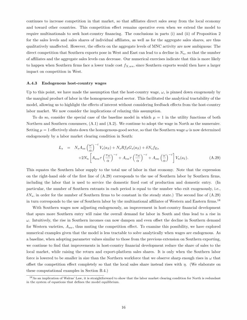
continues to increase competition in that market, so that affiliates direct sales away from the local economy

and toward other countries. This competition effect remains operative even when we extend the model to

require multinationals to seek host-country financing. The conclusions in parts (i) and (ii) of Proposition 2

for the sales levels and sales shares of individual affiliates, as well as for the aggregate sales shares, are thus

qualitatively unaffected. However, the effects on the aggregate levels of MNC activity are now ambiguous: The

direct competition that Southern exports pose in West and East can lead to a decline in Nn, so that the number

of affiliates and the aggregate sales levels can decrease. Our numerical exercises indicate that this is more likely

to happen when Southern firms face a lower trade cost fX,ws, since Southern exports would then have a larger

impact on competition in West.

A.4.3 Endogenous host-country wages

Up to this point, we have made the assumption that the host-country wage, ω, is pinned down exogenously by

the marginal product of labor in the homogeneous-good sector. This facilitated the analytical tractability of the

model, allowing us to highlight the effects of interest without considering feedback effects from the host-country

labor market. We now consider the implications of relaxing this assumption.

To do so, consider the special case of the baseline model in which µ = 1 in the utility functions of both

Northern and Southern consumers, (A.1) and (A.2). We continue to adopt the wage in North as the numeraire.

Setting µ = 1 effectively shuts down the homogenous-good sector, so that the Southern wage ω is now determined

endogenously by a labor market clearing condition in South:

Ls = NsAss

(ωα

)−εVs(aS) +NsRfSGs(aS) + δNsfEs

+2Nn

[Awwτ

(τωα

)−ε+Aewτ

(τωα

)−ε+Asw

(ωα

)−ε]Vn(aI). (A.29)

This equates the Southern labor supply to the total use of labor in that economy. Note that the expression

on the right-hand side of the first line of (A.29) corresponds to the use of Southern labor by Southern firms,

including the labor that is used to service the domestic fixed cost of production and domestic entry. (In

particular, the number of Southern entrants in each period is equal to the number who exit exogenously, i.e.,

δNs, in order for the number of Southern firms to be constant in the steady state.) The second line of (A.29)

in turn corresponds to the use of Southern labor by the multinational affiliates of Western and Eastern firms.18

With Southern wages now adjusting endogenously, an improvement in host-country financial development

that spurs more Southern entry will raise the overall demand for labor in South and thus lead to a rise in

ω. Intuitively, the rise in Southern incomes can now dampen and even offset the decline in Southern demand

for Western varieties, Asw, thus muting the competition effect. To examine this possibility, we have explored

numerical examples given that the model is less tractable to solve analytically when wages are endogenous. As

a baseline, when adopting parameter values similar to those from the previous extension on Southern exporting,

we continue to find that improvements in host-country financial development reduce the share of sales to the

local market, while raising the return and export-platform sales shares. It is only when the Southern labor

force is lowered to be smaller in size than the Northern workforce that we observe sharp enough rises in ω that

offset the competition effect completely so that the local sales share instead rises with η. (We elaborate on

these computational examples in Section B.4.)

18As an implication of Walras’ Law, it is straightforward to show that the labor market clearing condition for North is redundantin the system of equations that defines the model equilibrium.

16

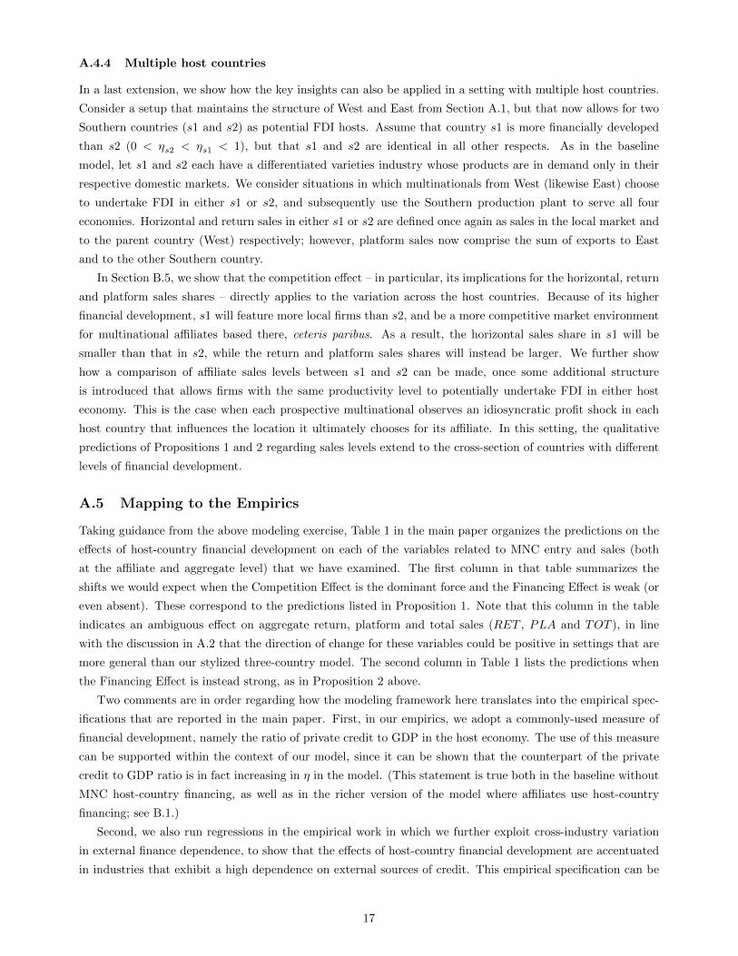
A.4.4 Multiple host countries

In a last extension, we show how the key insights can also be applied in a setting with multiple host countries.

Consider a setup that maintains the structure of West and East from Section A.1, but that now allows for two

Southern countries (s1 and s2) as potential FDI hosts. Assume that country s1 is more financially developed

than s2 (0 < ηs2 < ηs1 < 1), but that s1 and s2 are identical in all other respects. As in the baseline

model, let s1 and s2 each have a differentiated varieties industry whose products are in demand only in their

respective domestic markets. We consider situations in which multinationals from West (likewise East) choose

to undertake FDI in either s1 or s2, and subsequently use the Southern production plant to serve all four

economies. Horizontal and return sales in either s1 or s2 are defined once again as sales in the local market and

to the parent country (West) respectively; however, platform sales now comprise the sum of exports to East

and to the other Southern country.

In Section B.5, we show that the competition effect – in particular, its implications for the horizontal, return

and platform sales shares – directly applies to the variation across the host countries. Because of its higher

financial development, s1 will feature more local firms than s2, and be a more competitive market environment

for multinational affiliates based there, ceteris paribus. As a result, the horizontal sales share in s1 will be

smaller than that in s2, while the return and platform sales shares will instead be larger. We further show

how a comparison of affiliate sales levels between s1 and s2 can be made, once some additional structure

is introduced that allows firms with the same productivity level to potentially undertake FDI in either host

economy. This is the case when each prospective multinational observes an idiosyncratic profit shock in each

host country that influences the location it ultimately chooses for its affiliate. In this setting, the qualitative

predictions of Propositions 1 and 2 regarding sales levels extend to the cross-section of countries with different

levels of financial development.

A.5 Mapping to the Empirics

Taking guidance from the above modeling exercise, Table 1 in the main paper organizes the predictions on the

effects of host-country financial development on each of the variables related to MNC entry and sales (both

at the affiliate and aggregate level) that we have examined. The first column in that table summarizes the

shifts we would expect when the Competition Effect is the dominant force and the Financing Effect is weak (or

even absent). These correspond to the predictions listed in Proposition 1. Note that this column in the table

indicates an ambiguous effect on aggregate return, platform and total sales (RET , PLA and TOT ), in line

with the discussion in A.2 that the direction of change for these variables could be positive in settings that are

more general than our stylized three-country model. The second column in Table 1 lists the predictions when

the Financing Effect is instead strong, as in Proposition 2 above.

Two comments are in order regarding how the modeling framework here translates into the empirical spec-

ifications that are reported in the main paper. First, in our empirics, we adopt a commonly-used measure of

financial development, namely the ratio of private credit to GDP in the host economy. The use of this measure

can be supported within the context of our model, since it can be shown that the counterpart of the private

credit to GDP ratio is in fact increasing in η in the model. (This statement is true both in the baseline without

MNC host-country financing, as well as in the richer version of the model where affiliates use host-country

financing; see B.1.)

Second, we also run regressions in the empirical work in which we further exploit cross-industry variation

in external finance dependence, to show that the effects of host-country financial development are accentuated

in industries that exhibit a high dependence on external sources of credit. This empirical specification can be

17

justified within the context of the above modeling framework, if we view fS as capturing the degree of external

finance dependence of a particular industry: It can be shown that the cross-partial of each outcome variable of

interest with respect to η and fS will inherit the same sign as its partial derivative with respect to η. (See B.1

for the derivation of this property.)

B Detailed Derivations

B.1 Proofs for the Baseline Model

The FDI decision. We show that the two conditions, τω < 1 and fX < fD < fI , are sufficient to guarantee

that the optimal strategy for Western multinationals will be as follows: (i) highly productive Western firms

conduct FDI only in South but not in East; and (ii) Western multinationals use their Southern plant as a global

production center to serve all three markets.

Consider first a Western firm that already operates a multinational affiliate in South. It is then automatically

more profitable to use this affiliate as an export platform to East, rather than servicing East via direct exports

from West, or via direct FDI in East. This follows from the inequality:

(1− α)Aew

(τaωα

)1−ε−RfX > max

(1− α)Aew

(τaα

)1−ε−RfX , (1− α)Aew

( aα

)1−ε−RfI

,

which holds since τω < 1 < τ and fX < fI (bearing in mind that 1 − ε < 0). In particular, this rules out the

possibility of the MNC establishing affiliates in both South and East.

Next, conditional on setting up a Southern affiliate, we can further deduce that it is optimal to use this

affiliate to supply even the firm’s home market. This follows from:

(1− α)Aww

(τaωα

)1−ε−RfX > (1− α)Aww

( aα

)1−ε−RfD,

which holds since τω < 1 and fX < fD. Thus, it is more profitable to produce in South and export to West

than to incur the higher fixed cost and wages of production at home.

It remains to check that the optimal decision for a Western firm that becomes a multinational is to locate

its overseas affiliate in South, rather than in East. For this, we compare the total profits from servicing all

three countries out of an affiliate in South versus an affiliate in East:

(1− α)Aww

(τaωα

)1−ε−RfX + (1− α)Aew

(τaωα

)1−ε−RfX + (1− α)Asw

(aωα

)1−ε−RfI

> max

(1− α)Aww

( aα

)1−ε−RfD, (1− α)Aww

(τaα

)1−ε−RfX

+ (1− α)Aew

( aα

)1−ε−RfI + (1− α)Asw

(τaα

)1−ε−RfX .

Note that if FDI is undertaken in East, the home market (West) can be supplied either through domestic

production or exports from East, while South would be serviced by exports from either West or East. The

expression on the right-hand side of the above inequality captures total profits from this alternative production

mode. It is straightforward to check that the above inequality holds when τω < 1, ω < 1, ω < τ and fX < fD.

It is thus not optimal for a Western firm to conduct FDI in East.

In sum, the conditions τω < 1 and fX < fD < fI guarantee that the FDI decision is in effect a decision

over whether to relocate the firm’s global production center to South, with only headquarter activities retained

in West.

18

Proof of Lemma 1. Log-differentiating (A.13) and (A.15), one obtains:

(ε− 1)daSaS

=dη

η+dAssAss

, and

0 = aε−1S Vs(aS)

dAssAss

+ [aε−1S V ′s (aS)− ηG′s(aS)]daS .

To derive the second equation above, we used the fact that (1−α)Ass(ω/α)1−ε = (1/η)aε−1S RfSω, which holds

from the expression for a1−εS in (A.13). Solving these two equations simultaneously yields:

daSdη

=1

η

aε−1S Vs(aS)

(ε− 1)aε−2S Vs(aS) + [aε−1

S V ′s (aS)− ηG′s(aS)], and

dAssdη

= −Assη

aε−1S V ′s (aS)− ηG′s(aS)

(ε− 1)aε−2S Vs(aS) + [aε−1

S V ′s (aS)− ηG′s(aS)].

Applying Leibniz’s rule to Vs(aS) =∫ aS

0a1−εdGs(a), we have: aε−1

S V ′s (aS) = G′s(aS). Hence, aε−1S V ′s (aS) −

ηG′s(aS) = (1−η)G′s(aS) > 0, since η ∈ (0, 1) and G′s(a) > 0. Since ε > 1, it follows that daSdη > 0 and dAss

dη < 0.

While the above proof holds for any cdf Gs(a), it is straightforward to show for the case of the Pareto

distribution, Gs(a) = (a/as)k, that the above derivatives can be written more simply as:

daSdη

=aSη

1− ρSε− 1

, and (B.1)

dAssdη

= −AssηρS . (B.2)

Here, ρS is a constant that depends only on parameter values: ρS ≡(1−η) k−ε+1

ε−1

1+(1−η) k−ε+1ε−1

∈ (0, 1). These are convenient

expressions that we use frequently in the rest of the proofs.

Proof of Lemma 2. We take the remaining equations that define the industry equilibrium in West – (A.3)-

(A.4), (A.9)-(A.12), (A.14) and (A.16)-(A.19) – and differentiate them. First, log-differentiating (A.9)-(A.11)

yields:

(ε− 1)daDaD

=dAwwAww

, (B.3)

(ε− 1)daXNaXN

=dAewAew

, and (B.4)

(ε− 1)daXSaXS

=dAswAsw

. (B.5)

Since Asw = Ass, it immediately follows from (B.2) and (B.5) that dAswdη = dAss

dη < 0, and hence that:

1

aXS

daXSdη

= −1

η

ρSε− 1

< 0. (B.6)

This establishes part (iii) of the lemma.

We next differentiate the free-entry condition for West, (A.14):

19

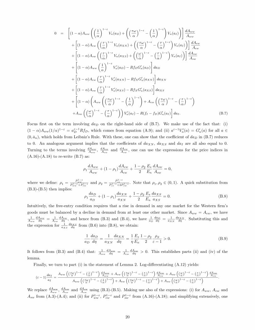
0 =

[(1− α)Aww

((1

α

)1−ε

Vn(aD) +

((τωα

)1−ε−(

1

α

)1−ε)Vn(aI)

)]dAwwAww

+

[(1− α)Aew

(( τα

)1−εVn(aXN ) +

((τωα

)1−ε−( τα

)1−ε)Vn(aI)

)]dAewAew

+

[(1− α)Asw

(( τα

)1−εVn(aXS) +

((ωα

)1−ε−( τα

)1−ε)Vn(aI)

)]dAswAsw

+

[(1− α)Aww

(1

α

)1−ε

V ′n(aD)−RfDG′n(aD)

]daD

+

[(1− α)Aew

( τα

)1−εV ′n(aXN )−RfXG′n(aXN )

]daXN

+

[(1− α)Asw

( τα

)1−εV ′n(aXS)−RfXG′n(aXS)

]daXS

+

[(1− α)

(Aww

((τωα

)1−ε−(

1

α

)1−ε)

+Aew

((τωα

)1−ε−( τα

)1−ε)+Asw

((ωα

)1−ε−( τα

)1−ε))V ′n(aI)−R(fI − fD)G′n(aI)

]daI . (B.7)

Focus first on the term involving daD on the right-hand side of (B.7). We make use of the fact that: (i)

(1 − α)Aww(1/α)1−ε = aε−1D RfD, which comes from equation (A.9); and (ii) aε−1V ′n(a) = G′n(a) for all a ∈

(0, an), which holds from Leibniz’s Rule. With these, one can show that the coefficient of daD in (B.7) reduces

to 0. An analogous argument implies that the coefficients of daXN , daXS and daI are all also equal to 0.

Turning to the terms involving dAwwAww

, dAewAew

and dAswAsw

, one can use the expressions for the price indices in

(A.16)-(A.18) to re-write (B.7) as:

ρ1

dAwwAww

+ (1− ρ1)dAewAew

+1− ρ2

2

EsEn

dAswAsw

= 0,

where we define: ρ1 =P 1−εww

P 1−εww +P 1−ε

ewand ρ2 =

P 1−εss

P 1−εss +2P 1−ε

sw. Note that ρ1, ρ2 ∈ (0, 1). A quick substitution from

(B.3)-(B.5) then implies:

ρ1

daDaD

+ (1− ρ1)daXNaXN

+1− ρ2

2

EsEn

daXSaXS

= 0. (B.8)

Intuitively, the free-entry condition requires that a rise in demand in any one market for the Western firm’s

goods must be balanced by a decline in demand from at least one other market. Since Aww = Aew, we have1

AwwdAwwdη = 1

AewdAewdη , and hence from (B.3) and (B.4), we have 1

aDdaDdη = 1

aXNdaXNdη . Substituting this and

the expression for 1aXS

daXSdη from (B.6) into (B.8), we obtain:

1

aD

daDdη

=1

aXN

daXNdη

=1

η

EsEn

1− ρ2

2

ρSε− 1

> 0. (B.9)

It follows from (B.3) and (B.4) that: 1Aww

dAwwdη = 1

AewdAewdη > 0. This establishes parts (ii) and (iv) of the

lemma.

Finally, we turn to part (i) in the statement of Lemma 2. Log-differentiating (A.12) yields:

(ε− 1)daI

aI=Aww

((τωα

)1−ε − ( 1α

)1−ε) dAwwAww

+Aew((

τωα

)1−ε − ( τα

)1−ε) dAewAew

+Asw((

ωα

)1−ε − ( τα

)1−ε) dAswAsw

Aww((

τωα

)1−ε − ( 1α

)1−ε)+Aew

((τωα

)1−ε − ( τα

)1−ε)+Asw

((ωα

)1−ε − ( τα

)1−ε) .

We replace dAwwAww

, dAewAewand dAsw

Aswusing (B.3)-(B.5). Making use also of the expressions: (i) for Aww, Aew and

Asw from (A.3)-(A.4); and (ii) for P 1−εww , P 1−ε

ew and P 1−εsw from (A.16)-(A.18); and simplifying extensively, one

20

can show that:

daIaI

=ρ1(1−∆1)daDaD + (1− ρ1)(1−∆2)daXNaXN

+ 1−ρ22

EsEn

(1−∆3)daXSaXS

ρ1(1−∆1) + (1− ρ1)(1−∆2) + 1−ρ22

EsEn

(1−∆3), (B.10)

where we define:

∆1 =

(1α

)1−εVn(aD)(

1α

)1−εVn(aD) + (

(τωα

)1−ε − ( 1α

)1−ε)Vn(aI)

,

∆2 =

(τα

)1−εVn(aXN )(

τα

)1−εVn(aXN ) + (

(τωα

)1−ε − ( τα)1−ε)Vn(aI), and

∆3 =

(τα

)1−εVn(aXS)(

τα

)1−εVn(aXS) + (

(ωα

)1−ε − ( τα)1−ε)Vn(aI).

Thus, daIaI

is a weighted average of daDaD

, daXNaXN

and daXSaXS

. Note that ∆1,∆2,∆3 ∈ (0, 1). Moreover, using the

above definitions, we have: sign∆1 −∆2 = sign(ω1−ε − 1)VN (aD)− ((τω)1−ε − 1)VN (aXN ) > 0. This

inequality holds as: VN (aD) > VN (aXN ) > 0 (since aD > aXN ), and ω1−ε− 1 > (τω)1−ε− 1 > 0. Analogously,

we have: sign∆2 −∆3 = sign(ω1−ε − τ1−ε)VN (aXN ) − ((τω)1−ε − τ1−ε)VN (aXS) > 0. This is again

positive as: VN (aXN ) > VN (aXS) > 0 (since aXN > aXS), and ω1−ε − τ1−ε > (τω)1−ε − τ1−ε > 0. In sum, we

have: 1 > ∆1 > ∆2 > ∆3 > 0. We further define: ∆d = ρ1(1−∆1) + (1− ρ1)(1−∆2) + 1−ρ22

EsEn

(1−∆3) > 0,

which is the denominator in (B.10). We now substitute into (B.10) the expressions for 1aXS

daXSdη , 1

aDdaDdη and

1aXN

daXNdη from (B.6) and (B.9). After simplifying, one obtains:

1

aI

daIdη

=1

η

1

∆d

EsEn

1− ρ2

2

ρSε− 1

[∆3 − ρ1∆1 − (1− ρ1)∆2] < 0. (B.11)

That this last expression is negative follows from the fact that ρ1, ρ2,∆1,∆2,∆3 ∈ (0, 1), and that ∆1 > ∆2 >

∆3. Moreover, (B.6) and (B.11) imply:

1

aI

daIdη− 1

aXS

daXSdη

=1

η

1

∆d

ρSε− 1

[EsEn

1− ρ2

2(∆3 − 1) + ∆d

]=

1

η

1

∆d

ρSε− 1

[ρ1(1−∆1) + (1− ρ1)(1−∆2)]

> 0.

Thus, 1aXS

daXSdη < 1

aIdaIdη < 0, which completes the proof of the lemma.

Proof of Proposition 1. Recall the definitions of HOR(a), PLA(a) and RET (a) from Section A.2. Lemma

2 then implies that when η improves, HOR(a) falls (since dAswdη < 0), PLA(a) increases (since dAew

dη > 0), and

RET (a) increases (since dAwwdη > 0). This establishes part (i) of the proposition.

For part (ii), from (A.23), one can see that ddη

HOR(a)TOT (a) < 0, since both Aww

Aswand Aew

Aswincrease with η. On

the other hand, from (A.24) and (A.25), we have ddη

PLA(a)TOT (a) = d

dηRET (a)TOT (a) > 0, since Asw

Aewis decreasing in η and

AwwAew

= 1.

For part (iii), we first need an expression for 1Nn

dNndη . Start by log-differentiating (A.3):

dAwwAww

= −ρ1

dP 1−εww

P 1−εww

− (1− ρ1)dP 1−ε

ew

P 1−εew

. (B.12)

21

Equations (A.16) and (A.17) in turn provide us with the log-derivatives of the two price indices that appear on

the right-hand side of (B.12):

dP 1−εww

P 1−εww

=dNnNn

+ (k − ε+ 1)

(∆1

daDaD

+ (1−∆1)daIaI

), and (B.13)

dP 1−εew

P 1−εew

=dNnNn

+ (k − ε+ 1)

(∆2

daXNaXN

+ (1−∆2)daIaI

). (B.14)

We now substitute: (i) from (B.13) and (B.14) into (B.12); (ii) from (B.3) into the left-hand side of (B.12); and

(iii) the expressions for 1aXS

daXSdη , 1

aDdaDdη and 1

aXNdaXNdη from (B.6) and (B.9) into (B.12). After some algebra,

this yields:

1

Nn

dNndη

=1

η

1

∆d

EsEn

1− ρ22

ρSε− 1

[−(ε− 1)∆d

−(k − ε+ 1)

(∆3(ρ1(1−∆1) + (1− ρ1)(1−∆2)) +

EsEn

1− ρ22

(1−∆3)(ρ1∆1 + (1− ρ1)∆2

)]< 0.

Note that we make use here of the fact that k−ε+1 > 0. As aI also decreases in response to an increase in η, it

follows that an improvement in Southern financial development decreases both the measure of Western/Eastern

firms, Nn, and the “number” of multinationals, NnGn(aI). The further effect that this has on aggregate platform

sales in (A.21) can be computed from:

d

dηlnPLA =

1

Nn

dNndη

+ (ε− 1)1

aXN

daXNdη

+ (k − ε+ 1)1

aI

daIdη

=1

η

1

∆d

EsEn

1− ρ22

ρSε− 1

(k − ε+ 1)[(∆3 − ρ1∆1 − (1− ρ1)∆2)

−(

∆3(ρ1(1−∆1) + (1− ρ1)(1−∆2)) +EsEn

1− ρ22

(1−∆3)(ρ1∆1 + (1− ρ1)∆2

)]< 0,

where recall from equation (B.11) that ∆3−ρ1∆1−(1−ρ1)∆2 is indeed negative. Looking back at the definitions

in (A.20)-(A.22), and making use of parts (iii) and (iv) of Lemma 2, we then have: ddη lnPLA = d

dη lnRET >ddη lnHOR. Hence, the aggregate sales levels HOR, PLA and RET all decrease in response to an improvement

in η.

Proof of Lemma 3. First, observe that the equilibrium for South’s differentiated varieties industry is still

determined by (A.13) and (A.15) as in the baseline model. Thus, Lemma 1 holds and the expressions for daSdη

and dAssdη from (B.1) and (B.2) still apply. As for the Western industry, only two equations are affected relative

to the baseline model when we differentiate the equilibrium system. The first of these is the equation obtained

from log-differentiating the new FDI cutoff, (A.26):

∆ddaIaI

=∆d

ε− 1

dη

η+ ρ1(1−∆1)

daDaD

+ (1− ρ1)(1−∆2)daXNaXN

+1− ρ2

2

EsEn

(1−∆3)daXSaXS

. (B.15)

The additional term, ∆d

ε−1dηη , on the right-hand side captures the direct effect that Southern financial develop-

ment has on Western firms. The second equation that is affected is the free-entry condition. In the manipulation

of (B.7), we now need to bear in mind that the coefficient of the term in daI is no longer equal to 0. This is

because:

22

(1 − α)

[Aww

(( τωα

)1−ε−(

1

α

)1−ε)

+Aew

(( τωα

)1−ε−( τα

)1−ε)+Asw

((ωα

)1−ε−( τα

)1−ε)]V ′n(aI)

−R(fI − fD)G′n(aI)

= (1 − α)(1 − η)

[Aww

(( τωα

)1−ε−(

1

α

)1−ε)

+Aew

(( τωα

)1−ε−( τα

)1−ε)+Asw

((ωα

)1−ε)]V ′n(aI)

where the last step follows from using the definition of a1−εI from (A.26) to substitute out for R(fI − fD), as

well as from using Leibniz’s rule to replace G′n(aI) with aε−1I V ′n(aI). We now follow analogous algebraic steps

as in the proof of Lemma 2, in particular, substituting in the definitions of the price indices (A.16)-(A.18), as

well as the definitions of ρ1 and ∆d. This allows us to rewrite the derivative of the free-entry condition as:

ρ1

daDaD

+ (1− ρ1)daXNaXN

+1− ρ2

2

EsEn

daXSaXS

+ (1− η)k − ε+ 1

ε− 1∆d

daIaI

= 0. (B.16)

Since the expression for a1−εXS in (A.11) remains unchanged, one can quickly see from the proof of Lemma 2

that we still have 1aXS

daXSdη = − 1

ηρSε−1 as in equation (B.6). Likewise, the same argument in the proof of Lemma

2 implies that 1aD

daDdη = 1

aXNdaXNdη . Substituting these two properties into (B.15) and (B.16), this leaves us

with a system of two linear equations in the two unknowns, 1aD

daDdη and 1

aIdaIdη . Solving these two equations

simultaneously then yields:

1

aI

daIdη

=1

η

1− ρTε− 1

[1− ρS

EsEn

1− ρ2

2

ρ1∆1 + (1− ρ1)∆2 −∆3

∆d

](B.17)

1

aD

daDdη

=1

η

[−ρT +

EsEn

1− ρ2

2(1− ρT )

(ρS − (1− ρS)(1− η)

k − ε+ 1

ε− 1(1−∆3)

)](B.18)

where ρT is defined by: ρT ≡(1−η) k−ε+1

ε−1 (ρ1(1−∆1)+(1−ρ1)(1−∆2))

1+(1−η) k−ε+1ε−1 (ρ1(1−∆1)+(1−ρ1)(1−∆2))

∈ (0, 1).

Examining (B.17), note that: (i) ρ1∆1 + (1 − ρ1)∆2 − ∆3 > 0, since ∆1,∆2 > ∆3; and moreover (ii)EsEn

1−ρ22 (ρ1∆1 + (1− ρ1)∆2 −∆3) < Es

En

1−ρ22 (1 − ∆3) < ∆d, since ∆1,∆2 < 1. These two facts imply that:

EsEn

1−ρ22

ρ1∆1+(1−ρ1)∆2−∆3

∆d∈ (0, 1). Since we also have ρS ∈ (0, 1), it follows from (B.17) that 1

aIdaIdη > 0, as

claimed in part (i) of Lemma 3. We have also already seen that: 1aXS

daXSdη = − 1

ηρSε−1 < 0, which is part (ii) of

the lemma.

As for (B.18), the sign of 1aD

daDdη = 1

aXNdaXNdη is in principle ambiguous: The two numerical examples in

footnote 15 illustrate that this derivative can be either positive or negative. We can nevertheless evaluate the

following:1

aD

daDdη− 1

aXS

daXSdη

=1

η

[ρS − ρT +

EsEn

1− ρ2

2(1−∆3)ρS(1− ρT )∆3

]. (B.19)

Using the definitions of ρS and ρT , we have: ρS − ρT = ρS(1 − ρT ) [1− ρ1(1−∆1)− (1− ρ1)(1−∆2)] > 0,

since: ρ1(1 − ∆1) + (1 − ρ1)(1 − ∆2) < ρ1 + (1 − ρ1) = 1, and ρS , ρT ∈ (0, 1). Inspecting (B.19), we have1aD

daDdη −

1aXS

daXSdη > 0, which establishes part (iii) of Lemma 3. As for parts (iv) and (v) of the lemma, these

follow immediately from applying (B.3)-(B.5).

Proof of Proposition 2. As in the proof of Proposition 1, ddηHOR(a), d

dηPLA(a) and ddηRET (a) respectively

inherit the signs of dAswdη , dAewdη and dAww

dη . Lemma 3 then implies that dAswdη > 0, but also that dAew

dη and dAwwdη

cannot be conclusively signed. This establishes part (i) of this proposition.

Furthermore, part (v) of Lemma 3 implies that AwwAsw

and AewAsw

are both increasing in η. Referring back

to the definitions of the sales shares in (A.23)-(A.25), we immediately have ddη

HOR(a)TOT (a) < 0 and d

dηPLA(a)TOT (a) =

23

ddη

RET (a)TOT (a) > 0. This pins down part (ii) of the proposition.

For part (iii), we first write down the derivatives of the aggregate variables of interest. Observe that the

expressions for the log-derivatives of Aww, P 1−εww and P 1−ε

ew in equations (B.12)-(B.14) remain valid in the model

with host-country financing. EliminatingdP 1−εww

P 1−εww

anddP 1−εew

P 1−εew

from these equations and using (B.3), we have:

1

Nn

dNndη

= −(ε− 1)daDaD− (k − ε+ 1)

[ρ1

(∆1

1

aD

daDdη

+ (1−∆1)1

aI

daIdη

)+(1− ρ1)

(∆2

1

aXN

daXNdη

+ (1−∆2)1

aI

daIdη

)]. (B.20)

In turn, how the number of multinationals, NnGn(aI), responds to η is given by: ddη logNnGn(aI) = 1

NndNndη +

G′n(aI)aIGn(aI)

1aI

daIdη = 1

NndNndη + k 1

aIdaIdη , where

G′n(a)aGn(a) = k for the Pareto distribution. Using (B.20), together with

the fact that 1aD

daDdη = 1

aXNdaXNdη , this yields:

1

Nn

dNndη

+ k1

aI

daIdη

= [−(ε− 1)− (k − ε+ 1) (ρ1∆1 + (1− ρ1)∆2)]1

aD

daDdη

+ [k − (k − ε+ 1) (ρ(1−∆1) + (1− ρ1)(1−∆2))]1

aI

daIdη

= [(ε− 1) + (k − ε+ 1) (ρ1∆1 + (1− ρ1)∆2)]

(1

aI

daIdη− 1

aD

daDdη

). (B.21)

Note that it is straightforward to verify that: (ε − 1) + (k − ε + 1) (ρ1∆1 + (1− ρ1)∆2) = k − (k − ε +

1) (ρ(1−∆1) + (1− ρ1)(1−∆2)) > 0. It thus suffices to determine the sign of 1aI

daIdη −

1aD

daDdη . For this,

substitute in the expressions for these derivatives from (B.17) and (B.18). Some algebra leads to:

1

aI

daIdη− 1

aD

daDdη

=1

η

1

ε− 1

[1− ρS(1− ρT )

EsEn

1−ρ22

(1−∆3)

∆d

(ρ1∆1 + (1− ρ1)∆2 +

EsEn

1− ρ22

∆3

)]. (B.22)

As for the effect on aggregate horizontal sales, we differentiate (A.20) with respect to η. Making use of

(B.5), we have:

d

dηlnHOR =

1

Nn

dNndη

+ (ε− 1)1

aXS

daXSdη

+ (k − ε+ 1)1

aI

daIdη

=1

Nn

dNndη

+ k1

aI

daIdη− (ε− 1)

(1

aD

daDdη− 1

aXS

daXSdη

)− (ε− 1)

(1

aI

daIdη− 1

aD

daDdη

)=

1

η

[1− ρS(1− ρT )

EsEn

1−ρ22

(1−∆3)

∆d

(ρ1∆1 + (1− ρ1)∆2 +

EsEn

1− ρ22

∆3

)

−ρS(1− ρT )ρ1∆1 + (1− ρ1)∆2 + Es

En

1−ρ22

∆3

k−ε+1ε−1

(ρ1∆1 + (1− ρ1)∆2)

]. (B.23)

Note that in the penultimate step, we substituted in for 1Nn

dNndη + k 1

aIdaIdη using (B.21), for 1

aDdaDdη −

1aXS

daXSdη

using (B.19), for 1aI

daIdη −

1aD

daDdη using (B.22), and then simplified extensively.

Likewise, differentiating (A.21) with respect to η and using (B.3), we have:

d

dηlnPLA =

d

dηlnRET =

1

Nn

dNndη

+ (ε− 1)1

aD

daDdη

+ (k − ε+ 1)1

aI

daIdη

=1

Nn

dNndη

+ k1

aI

daIdη− (ε− 1)

(1

aI

daIdη− 1

aD

daDdη

)= (k − ε+ 1) (ρ1∆1 + (1− ρ1)∆2)

(1

aI

daIdη− 1

aD

daDdη

). (B.24)

Once again, we have made use of the expression for 1Nn

dNndη +k 1

aIdaIdη in (B.21) to arrive at (B.24). In particular,

observe from (B.21) and (B.24) that the measure of multinationals, aggregate platform sales and aggregate

24

return sales all move in the same direction when η changes.

It remains for us to analyze the sign of the derivatives in (B.21), (B.23) and (B.24). Recall the definition:

ρS ≡(1−η) k−ε+1

ε−1

1+(1−η) k−ε+1ε−1

. When η = 1, we thus have ρS = 0, in which case it quickly follows from (B.22) that

1aI

daIdη −

1aD

daDdη > 0, and hence that d

dη lnNnGn(aI),ddη lnPLA, ddη lnRET > 0. Moreover, inspecting (B.23),

we would also have ddη lnHOR > 0. By continuity, it follows that d

dη lnNnGn(aI),ddη lnHOR, d

dη lnPLA andddη lnRET must all be positive in a neighborhood of η, so that NnGn(aI), HOR, PLA and RET are increasing

in host-country financial development if the initial level of η is sufficiently high. This establishes part (iii) of

the proposition.

It is useful to point out here that some form of a sufficient condition is indeed required in the statement of

part (iii) of the proposition. Examining the expression for 1aI

daIdη −

1aD

daDdη in (B.22) more closely, one can see

that ρS , 1−ρT , EsEn1−ρ2

2 (1−∆3)/∆d ∈ (0, 1), but that we cannot explicitly bound ρ1∆1+(1−ρ1)∆2+ EsEn

1−ρ22 ∆3

between 0 and 1, even though ∆1,∆2,∆3 ∈ (0, 1). That said, it is actually not easy to find parameter values

for which NnGn(aI), HOR, PLA or RET end up decreasing in η, even when we set the initial level of η to be

very small. As an example, consider the set of parameter values: R = 1.07, ε = 3.8, Ln = Ls = 1, fD = 0.2,

fX = 0.15, fS = 0.1, fEn = fEs = 1, τ = 1.3, ω = 0.7, aN = aS = 25, k = 4, δ = 0.1, µ = 0.5 and η = 0.01.

While this features a low η, it turns out that it is also necessary to set the remaining parameter fI to be very

high to generate a counter-example to part (iii) of the proposition. In particular, when fI = 1000, we have an

equilibrium with aD = 14.41, aXN = 12.28, aXS = 12.23 and aI = 0.20, in which ddηHOR = −0.89 < 0. This

value of fI is of course exceedingly large relative to the other fixed cost parameters. But attempting to reduce

the value of fI to 100 results in an equilibrium in which the order of two of the cutoffs gets reversed, specifically

aXN = 12.18 and aXS = 12.23.

The relationship between private credit and η. Consider first the baseline model where MNCs do not

require host-country financing. The model counterpart of our empirical measure of private credit over GDP is:

NsG(aS)fSω/(ωL), this being the total amount borrowed by domestic firms, divided by the total labor income

in South. Since fS , ω, and L are fixed, our task is to show that NsGs(aS), the “number” of successful entrants

in the Southern industry, is increasing in η.

First, log-differentiate the ideal price index, P 1−εss , given by (A.19):

1

Ns

dNsdη

=1

P 1−εss

dP 1−εss

dη− (k − ε+ 1)

1

aS

daSdη

. (B.25)

We therefore have: ddη logNsGs(aS) = 1

NsdNSdη +

G′s(aS)aSGs(aS)

1aS

daSdη = 1

NsdNSdη +k 1

aSdaSdη = 1

P 1−εss

dP 1−εss

dη +(ε−1) 1aS

daSdη ,

where we have made use of (B.25) to obtain the last expression. We have seen from Lemma 1 that daSdη > 0.

As ε > 1, it will thus suffice to show that 1P 1−εss

dP 1−εss

dη > 0, in order to conclude that ddη logNsGs(aS) > 0.

For this, we log-differentiate (A.4) to obtain: dAswAsw

= −ρ2dP 1−εss

P 1−εss

− (1 − ρ2)dP 1−εsw

P 1−εsw

. Substituting in the

expression for dAswAsw

from (B.5) into this last equation, and rearranging, gives:

ρ2

1

P 1−εss

dP 1−εss

dη= −(ε− 1)

1

aXS

daXSdη

− (1− ρ2)1

P 1−εsw

dP 1−εsw

dη. (B.26)

Now, log-differentiating (A.18) yields:

1

P 1−εsw

dP 1−εsw

dη=

1

Nn

dNndη

+ (k − ε+ 1)

(∆3

1

aXS

daXSdη

+ (1−∆3)1

aI

daIdη

). (B.27)

25

Since 1aXS

daXSdη < 0 and 1

aIdaIdη < 0 from Lemma 2, and 1

NndNndη < 0 from Proposition 1, it follows that:

1P 1−εsw

dP 1−εsw

dη < 0. From (B.26), we immediately have: 1P 1−εss

dP 1−εss

dη > 0, so that ddη logNsGs(aS) > 0, and we

indeed have total private credit extended in South increasing with η in our baseline model.

As for the extension with local borrowing by MNCs, the private credit to GDP ratio in South is now given

instead by: [2NnGn(aI)(fI − fD) +NsGs(aS)fSω]/(ωL), where the numerator takes into account total lending

to multinational affiliates from both East and West, as well as to Southern domestic firms. Under the sufficient

condition assumed for part (iii) of Proposition 2 – that the initial level of host-country financial development be

sufficiently high – we have already seen that the “number” of multinational affiliates NnG(aI) will be increasing

in η. We now show that when the initial level of η is sufficiently high, this increase in 2NnGn(aI) will dominate

any movements in NsGs(aS) in the numerator of the private credit to GDP ratio.

Log-differentiating the expression for the private credit to GDP ratio, we get:

2(dNndη

Gn(aI) +NnG′n(aI)

daIdη

)(fI − fD) +

(dNsdηGs(aS) +NsG

′s(aS) daS

dη

)fSω

2NnGn(aI)(fI − fD) +NsGs(aS)fSω

=2NnGn(aI)(fI − fD)

(1Nn

dNndη

+ k 1aI

daIdη

)+NsGs(aS)fSω

(1Ns

dNsdη

+ k 1aS

daSdη

)2NnGn(aI)(fI − fD) +NsGs(aS)fSω

∝(

1

Nn

dNndη

+ k1

aI

daIdη

)+

NsGs(aS)fSω

2NnGn(aI)(fI − fD)

(1

Ns

dNsdη

+ k1

aS

daSdη

), (B.28)

where ‘∝’ denotes equality up to a positive multiplicative term. We thus focus on pinning down the sign of

(B.28) in the neighborhood of η = 1. Using (B.21) and (B.22), and setting η = 1, we have: 1Nn

dNndη + k 1

aIdaIdη =

1 + k−ε+1ε−1 (ρ1∆1 + (1− ρ1)∆2). Next, since (A.4), (A.18) and (A.19) are unchanged in the extension with

host-country financing, equations (B.25), (B.26) and (B.27) remain valid, so that:

1

Ns

dNs

dη+ k

1

aS

daS

dη= −

ε− 1

ρ2

1

aXS

daXS

dη−

1 − ρ2ρ2

1

P 1−εsw

dP 1−εsw

dη+ (ε− 1)

1

aS

daS

dη

= −ε− 1

ρ2

1

aXS

daXS

dη+ (ε− 1)

1

aS

daS

dη

−1 − ρ2ρ2

(1

Nn

dNn

dη+ k

1

aI

daI

dη+ (k − ε+ 1)

(∆3

1

aXS

daXS

dη+ (1 − ∆3)

1

aI

daI

dη

)− k

1

aI

daI

dη

).

We now make use of the following properties: (i) 1−ρ2ρ2

=2P 1−εsw

P 1−εss

from the definition of ρ2; (ii) 1aS

daSdη = 1

η1−ρSε−1

from (B.1); (iii) 1aXS

daXSdη = − 1

ηρSε−1 from the proof of Lemma 3; (iv) the expression for 1

NndNndη + k 1

aIdaIdη in

(B.21); and (v) the expression for 1aI

daIdη in (B.17). Evaluating these at η = 1 and following some algebra, one

obtains: 1Ns

dNsdη + k 1

aSdaSdη = 1− 2P 1−ε

sw

P 1−εss

k−ε+1ε−1 (ρ1∆1 + (1− ρ1)∆2 −∆3). We further use the expressions for the

ideal price indices in (A.18) and (A.19) to simplify the following:

NsGs(aS)fSω

2NnGn(aI)(fI − fD)

2P 1−εsw

P 1−εss

=(Gs(aS)/Vs(aS))fSω

(Gn(aI)/Vn(aI))(fI − fD)

1

1−∆3

ω1−ε − τ1−ε

ω1−ε

=fSω/a

1−εS

(fI − fD)/a1−εI

1

1−∆3

ω1−ε − τ1−ε

ω1−ε

=Ass(ω

1−ε − τ1−ε)Aww((τω)1−ε − 1) +Aew((τω)1−ε − τ1−ε) +Asw(ω1−ε − τ1−ε)

1

1−∆3,

where we have substituted in the expressions for a1−εS in (A.13) and a1−ε

I in (A.26) for this last step. Since

Ass = Asw, we thus have: NsGs(aS)fSω2NnGn(aI)(fI−fD)

2P 1−εsw

P 1−εss

< 11−∆3

.

Applying the above properties to (B.28), we find that evaluated at η = 1:

26

(1

Nn

dNndη

+ k1

aI

daIdη

)+

NsGs(aS)fSω

2NnGn(aI)(fI − fD)

(1

Ns

dNsdη

+ k1

aS

daSdη

)= 1 +

k − ε+ 1

ε− 1(ρ1∆1 + (1− ρ1)∆2) +

NsGs(aS)fSω

2NnGn(aI)(fI − fD)

(1− 2P 1−ε

sw

P 1−εss

k − ε+ 1

ε− 1(ρ1∆1 + (1− ρ1)∆2 −∆3)

)>

k − ε+ 1

ε− 1(ρ1∆1 + (1− ρ1)∆2)− 1

1−∆3

k − ε+ 1

ε− 1(ρ1∆1 + (1− ρ1)∆2 −∆3)

∝ (ρ1∆1 + (1− ρ1)∆2) (1−∆3)− (ρ1∆1 + (1− ρ1)∆2 −∆3)

= ∆3 (1− ρ1∆1 − (1− ρ1)∆2) .

But this last expression is clearly positive, since ∆1,∆2 ∈ (0, 1). By a continuity argument, this allows us

to conclude that [2NnGn(aI)(fI − fD) + NsGs(aS)fSω]/(ωL) is increasing in η when the initial level of η is

sufficiently high.

Cross-industry heterogeneity. We show that the effects of host-country financial development in our

model will hold particularly for industries that have a higher financing requirement, as captured by fS . Under

the assumption that firm productivities within each industry follow a Pareto distribution, we have from (B.1)

and (B.2) that sign(d2aSdηdfS

)= sign

(daSdfS

)and sign

(d2AssdηdfS

)= −sign

(dAssdfS

). To pin down the signs of these

derivatives with respect to fS , we totally differentiate (A.13) and (A.15) to obtain:

(ε− 1)daSaS

= −dfSfS

+dAssAss

, and

0 = aε−1S Vs(aS)

dAssAss

+(aε−1S V ′s (aS)− ηG′s(aS)

)daS − ηGs(aS)

dfSfS

= aε−1S Vs(aS)

dAssAss

+ (1− η)aSG′s(aS)

daSaS− ηGs(aS)

dfSfS

.

Note that we have applied Leibniz’s rule to the definition of Vs(aS), as in the proof of Lemma 1, in the last

step above. Solving these two equations simultaneously yields:

1

aS

daSdfS

= − 1

fS

aε−1S Vs(aS)− ηGs(aS)

(ε− 1)aε−1S Vs(aS) + (1− η)aSG′s(aS)

, and

1

Ass

dAssdfS

=1

fS

[1−

(ε− 1)aε−1S Vs(aS)− (ε− 1)ηGs(aS)

(ε− 1)aε−1S Vs(aS) + (1− η)aSG′s(aS)

].

Looking at the numerator on the right-hand side of the above expression for 1aS

daSdfS

, observe that: aε−1S Vs(aS) =

aε−1S

∫ aS0

a1−εG′s(a)da = aε−1S

[a1−εS Gs(aS)−

∫ aS0

(1− ε)a−εGs(a)da]> ηGs(aS), which implies that 1

aSdaSdfS

<

0. Next, from the equation for 1Ass

dAssdfS

, we have: 0 < (ε−1)aε−1S Vs(aS)−(ε−1)ηGs(aS) < (ε−1)aε−1

S Vs(aS)+

(1− η)aSG′s(aS), which in turn means that 1

AssdAssdfS

> 0.

We can thus conclude that d2aSdηdfS

< 0 and d2AssdηdfS

< 0. In particular, the fact that d2AssdηdfS

inherits the same

negative sign as dAssdη is crucial, as it also means that sign

(d2AswdηdfS

)= sign

(dAswdη

). The effects of host-country

financial development on the market demand levels, and hence the respective sales shares in (A.23)-(A.25), are

therefore stronger in industries with a higher fS .

B.2 Model Extension: Home-bias in consumption

We establish that Proposition 1 in our baseline model continues to apply in this extension. We also provide

the proof of Proposition 3, which allows for a differential response of platform versus return sales to changes in

27

host-country financial development.

Model Setup. Recall that we modify the utility functions for n = w, e (West and East) and for s (South) to:

Un = y1−µn

∑j∈e,w

(∫Ωnj

xnj(a)α dGj(a)

) βα

µβ

, and (B.29)

Us = y1−µs

∑j∈e,w,s

(∫Ωsj

xsj(a)α dGj(a)

) βα

µβ

, (B.30)

where 0 < β < α < 1. We denote the elasticity of substitution for varieties from the same country by ε = 11−α ,

and the elasticity of substitution for varieties from different countries by φ = 11−β . Note that ε > φ > 1, so

that varieties from the same country are closer substitutes than varieties drawn from different countries.

Maximizing (B.29) and (B.30) subject to the standard budget constraints, one obtains that demand in

country i for a variety from country j is: xij(a) = Aijpij(a)−ε. The aggregate market demand levels are now

given by:

Aww = Aee =µEnP

ε−φww

P 1−φww + P 1−φ

ew

, (B.31)

Aew = Awe =µEnP

ε−φew

P 1−φww + P 1−φ

ew

, (B.32)

Asw = Ase =µEsP

ε−φsw

P 1−φss + 2P 1−φ

sw

, and (B.33)

Ass =µEsP

ε−φss

P 1−φss + 2P 1−φ

sw

. (B.34)

In contrast to the baseline model, we no longer have Aww = Aew and Asw = Ass. This is precisely due to the

introduction of the additional elasticity of substitution, φ. In particular, when ε = φ, the above collapses back

to the demand expressions from our baseline model.

The rest of the equations for the equilibrium system remain the same as in the baseline model. For com-

pleteness, we reproduce them below:

28

a1−εD =RfD

(1− α)Aww(1/α)1−ε(B.35)

a1−εXN =RfX

(1− α)Aew(τ/α)1−ε(B.36)

a1−εXS =RfX

(1− α)Asw(τ/α)1−ε(B.37)

a1−εI =R(fI − fD)

(1− α)[Aww(( τωα

)1−ε − ( 1α

)1−ε) +Aew(( τωα

)1−ε − ( τα

)1−ε) +Asw((ωα

)1−ε − ( τα

)1−ε)](B.38)

a1−εS =1

η

RfSω

(1− α)Ass(ω/α)1−ε(B.39)

δfEn = (1− α)Aww

(1

α

)1−ε

(Vn(aD)− Vn(aI))−RfD(Gn(aD)−Gn(aI))

+(1− α)Aew( τα

)1−ε(Vn(aXN )− Vn(aI))−RfX(Gn(aXN )−Gn(aI))

+(1− α)Asw( τα

)1−ε(Vn(aXS)− Vn(aI))−RfX(Gn(aXS)−Gn(aI))

+(1− α)

(Aww

(τωα

)1−ε+Aew

(τωα

)1−ε+Asw

(ωα

)1−ε)Vn(aI)−R(fI + 2fX)Gn(aI) (B.40)

δfEsω = (1− α)Ass(ωα

)1−εVs(aS)−RfSωGs(aS) (B.41)

P 1−εww = Nn

[(1

α

)1−ε

(Vn(aD)− Vn(aI)) +(τωα

)1−εVn(aI)

](B.42)

P 1−εew = Nn

[( τα

)1−ε(Vn(aXN )− Vn(aI)) +

(τωα

)1−εVn(aI)

](B.43)

P 1−εsw = Nn

[( τα

)1−ε(Vn(aXS)− Vn(aI)) +

(ωα

)1−εVn(aI)

](B.44)

P 1−εss = Ns

[(ωα

)1−εVs(aS)

](B.45)

The equilibrium is thus pinned down by the 15 equations (B.31)-(B.45) in the 15 endogeneous variables:

Aww, Aew, Asw, Ass, aD, aXN , aXS , aI , aS , Nn, Ns, Pww, Pew, Psw and Pss.

Proposition 1 continues to hold. It is clear that (B.39) and (B.41) once again pin down the equilibrium

for South’s differentiated varieties industry. Since these equations are unchanged from the baseline model, this

means that Lemma 1 holds, namely that daSdη > 0 and dAss

dη < 0.

We next show that a modified version of Lemma 2 now describes the subsequent impact on the industry

equilibrium in West (and East):

Lemma 2A: In the extended model with home-bias in consumption, (i) 1aXS

daXSdη < 1

aIdaIdη < 0; (ii)

1aXN

daXNdη > 1

aDdaDdη > 0; (iii) 1

AswdAswdη < 0; and (iv) 1

AewdAewdη > 1

AwwdAwwdη > 0.

In response to a small increase in η, we now have the proportional shift in the aXN cutoff exceeding that in the

aD cutoff, and hence the proportional increase in Aew exceeding that in Aww.

We proceed to prove this modified lemma. To provide a heuristic roadmap, we will take the remaining

13 equations that define the Western industry equilibrium – (B.31)-(B.33), (B.35)-(B.38), (B.40), and (B.42)-

(B.45) – and log-differentiate them. We then reduce the resulting system to a set of four equations in the four

unknowns, daDaD

, daXNaXN

, daXSaXS

and daIaI

. From this, we can determine the comparative statics with respect to η

for the Western industry cutoffs, and hence for the other endogenous variables as well.

29

First, log-differentiating (B.35), (B.36) and (B.37) yields:

(ε− 1)daDaD

=dAwwAww

, (B.46)

(ε− 1)daXNaXN

=dAewAew

, and (B.47)

(ε− 1)daXSaXS

=dAswAsw

. (B.48)

Since ε > 1, this implies: sign(daDdη ) = sign(dAwwdη ), sign(daXNdη ) = sign(dAewdη ), and sign(daXSdη ) = sign(dAswdη ).

Similarly, log-differentiating (B.38) yields:

(ε− 1)daI

aI=Aww

((τωα

)1−ε − ( 1α

)1−ε) dAwwAww

+Aew((

τωα

)1−ε − ( τα

)1−ε) dAewAew

+Asw((

ωα

)1−ε − ( τα

)1−ε) dAswAsw

Aww((

τωα

)1−ε − ( 1α

)1−ε)+Aew

((τωα

)1−ε − ( τα

)1−ε)+Asw

((ωα

)1−ε − ( τα

)1−ε) .

We replace dAwwAww

, dAewAew

and dAswAsw

by the expressions in (B.46)-(B.48). Making use also of the expressions for

Aww, Aew and Asw from (B.31)-(B.33), and for P 1−εww , P 1−ε

ew and P 1−εsw from (B.42)-(B.44), and simplifying

extensively, one can show that:

daIaI

=ρ1(1−∆1) daD

aD+ (1− ρ1)(1−∆2) daXN

aXN+ 1−ρ2

2EsEn

(1−∆3) daXSaXS

ρ1(1−∆1) + (1− ρ1)(1−∆2) + 1−ρ22

EsEn

(1−∆3), (B.49)

where we now define: ρ1 =P 1−φww

P 1−φww +P 1−φ

ewand ρ2 =

P 1−φss

P 1−φss +2P 1−φ

sw. Note that in contrast to the proof for the baseline

model, the definitions of ρ1 and ρ2 now involve φ, instead of ε. We nevertheless still have ρ1, ρ2 ∈ (0, 1). Recall

also the following definitions, which we retain from the proof for the baseline model:

∆1 =

(1α

)1−εVn(aD)(

1α

)1−εVn(aD) + (

(τωα

)1−ε − ( 1α

)1−ε)Vn(aI)

, (B.50)

∆2 =

(τα

)1−εVn(aXN )(

τα

)1−εVn(aXN ) + (

(τωα

)1−ε − ( τα

)1−ε)Vn(aI)

, and (B.51)

∆3 =

(τα

)1−εVn(aXS)(

τα

)1−εVn(aXS) + (

(ωα

)1−ε − ( τα

)1−ε)Vn(aI)

. (B.52)

Note that in the proof of Lemma 2, we showed that 1 > ∆1 > ∆2 > ∆3 > 0.

Next, we differentiate the free-entry condition for West, (B.40). Following the algebraic manipulations used

in the proof of Lemma 2, we once again obtain:

ρ1

daDaD

+ (1− ρ1)daXNaXN

+1− ρ2

2

EsEn

daXSaXS

= 0. (B.53)

A quick implication is that the three cutoffs aD, aXN and aXS cannot all move in the same direction.

We move on to log-differentiate the market demand expressions in (B.31)-(B.34):

dAwwAww

=

((1− ρ1)

φ− 1

ε− 1− 1

)dP 1−ε

ww

P 1−εww

− (1− ρ1)φ− 1

ε− 1

dP 1−εew

P 1−εew

, (B.54)

dAewAew

=

(ρ1φ− 1

ε− 1− 1

)dP 1−ε

ew

P 1−εew

− ρ1φ− 1

ε− 1

dP 1−εww

P 1−εww

, (B.55)

dAswAsw

=

(ρ2φ− 1

ε− 1− 1

)dP 1−ε

sw

P 1−εsw

− ρ2φ− 1

ε− 1

dP 1−εss

P 1−εss

, and (B.56)

dAssAss

=

((1− ρ2)

φ− 1

ε− 1− 1

)dP 1−ε

ss

P 1−εss

− (1− ρ2)φ− 1

ε− 1

dP 1−εsw

P 1−εsw

. (B.57)

Meanwhile, log-differentiating the ideal price indices (B.42)-(B.44) gives us:

30

dP 1−εww

P 1−εww

=dNnNn

+ (k − ε+ 1)

(∆1

daDaD

+ (1−∆1)daIaI

), (B.58)

dP 1−εew

P 1−εew

=dNnNn

+ (k − ε+ 1)

(∆2

daXNaXN

+ (1−∆2)daIaI

), and (B.59)

dP 1−εsw

P 1−εsw

=dNnNn

+ (k − ε+ 1)

(∆3

daXSaXS

+ (1−∆3)daIaI

), (B.60)

where we have made use of the fact thataV ′n(a)Vn(a) = k − ε+ 1 for the Pareto distribution.

Using Cramer’s Rule, we now invert (B.56) and (B.57) to obtain:

dP 1−εsw

P 1−εsw

=

(−ρ2

φ− 1

ε− φ − 1

)dAswAsw

+ ρ2φ− 1

ε− φdAssAss

, and (B.61)

dP 1−εss

P 1−εss

=

(−(1− ρ2)

φ− 1

ε− φ − 1

)dAssAss

+ (1− ρ2)φ− 1

ε− φdAswAsw

. (B.62)

Setting (B.60) equal to (B.61) then implies:

dNnNn

= ρ2φ− 1

ε− φdAssAss

−[(ε− 1)

(ρ2φ− 1

ε− φ + 1

)+ (k − ε+ 1)∆3

]daXSaXS

− (k − ε+ 1)(1−∆3)daIaI

. (B.63)

We now plug this expression for dNnNn

into (B.58) and (B.59), and substitute the subsequent expressions fordP 1−εww

P 1−εww

anddP 1−εew

P 1−εew

into (B.54) and (B.55). Finally, replacing dAwwAww

and dAewAew

with the expressions in terms ofdaDaD

and daXNaXN

from (B.46) and (B.47) respectively, one obtains after some rearrangement:

ρ2k − ε+ 1

φ− 1

ε− φdAssAss

=

[((1− ρ1)

φ− 1

ε− 1− 1

)∆1 −

ε− 1

k − ε+ 1

]daDaD− (1− ρ1)

φ− 1

ε− 1∆2

daXNaXN

+

[ε− 1

k − ε+ 1

(ρ2φ− 1

ε− φ + 1

)+ ∆3

]daXSaXS

+

[(∆1 −∆3)− (∆1 −∆2)(1− ρ1)

φ− 1

ε− 1

]daIaI

, and (B.64)

ρ2k − ε+ 1

φ− 1

ε− φdAssAss

= −ρ1φ− 1

ε− 1∆1

daDaD

+

[(ρ1φ− 1

ε− 1− 1

)∆2 −

ε− 1

k − ε+ 1

]daXNaXN

+

[ε− 1

k − ε+ 1

(ρ2φ− 1

ε− φ + 1

)+ ∆3

]daXSaXS

+

[(∆2 −∆3) + (∆1 −∆2)ρ1

φ− 1

ε− 1

]daIaI

. (B.65)

(B.49), (B.53), (B.64), and (B.65) give us four equations in the four unknowns, daDaD

, daXNaXN

, daXSaXS

and daIaI

.

To pin down the comparative statics explicitly, note that equating (B.65) and (B.64) implies:

daIaI

=1

∆1 −∆2

[(∆1 +

ε− 1

k − ε+ 1

ε− 1

ε− φ

)daDdD−(

∆2 +ε− 1

k − ε+ 1

ε− 1

ε− φ

)daXNdXN

]. (B.66)

Meanwhile, using (B.53) to eliminate daXSaXS

from (B.49) delivers:

daIaI

= −ρ1(∆1 −∆3)daDaD + (1− ρ1)(∆2 −∆3)daXNaXN

ρ1(1−∆1) + (1− ρ1)(1−∆2) + 1−ρ22

EsEn

(1−∆3). (B.67)

For convenience, let us define: ∆d = ρ1(1 − ∆1) + (1 − ρ1)(1 − ∆2) + 1−ρ22

EsEn

(1 − ∆3) > 0, which is the

denominator in (B.67). Then, setting (B.66) equal to (B.67) and rearranging, one obtains:

31

0 =

[ρ1(∆1 −∆3)(∆1 −∆2) + ∆d

(∆1 +

ε− 1

k − ε+ 1

ε− 1

ε− φ

)]daDaD

+

[(1− ρ1)(∆2 −∆3)(∆1 −∆2)−∆d

(∆2 +

ε− 1

k − ε+ 1

ε− 1

ε− φ

)]daXNaXN

. (B.68)

Since ∆1 − ∆2,∆1 − ∆3 > 0, it follows that the coefficient of daDaD

in (B.68) is positive. Moreover, using the

definition of ∆d, one can see that the coefficient of daXNaXNis strictly smaller than: (1−ρ1)(∆2−∆3)(∆1−∆2)−

(1 − ρ1)(1 −∆2)∆2, which itself is already negative, since: 1 −∆2 > ∆1 −∆2 > 0, and ∆2 > ∆2 −∆3 > 0.

Thus, the coefficient of daXNaXN

in (B.68) is negative. Since the linear combination in (B.68) is equal to 0, it

follows that sign(daDdη ) = sign(daXNdη ).

We require one more equation in daDaD

and daXNaXN

in order to pin down their common sign. For this, substitute

the expression for daIaI

from (B.67) and that for daXSaXS

from (B.53) into (B.64) to obtain:

ρ2k − ε+ 1

φ− 1

ε− φdAssAss

=

[((1− ρ1)

φ− 1

ε− 1− 1

)∆1 −

2ρ11− ρ2

EnEs

(ε− 1

k − ε+ 1

(ρ2φ− 1

ε− φ + 1

)+ ∆3

)− ε− 1

k − ε+ 1−(

(∆1 −∆3)− (∆1 −∆2)(1− ρ1)φ− 1

ε− 1

)ρ1(∆1 −∆3)

∆d

]daDaD

+

[−(1− ρ1)

φ− 1

ε− 1∆2 −

2(1− ρ1)

1− ρ2EnEs

(ε− 1

k − ε+ 1

(ρ2φ− 1

ε− φ + 1

)+ ∆3

)−(

(∆1 −∆3)− (∆1 −∆2)(1− ρ1)φ− 1

ε− 1

)(1− ρ1)(∆2 −∆3)

∆d

]daXNaXN

. (B.69)

Note that (∆1 − ∆3) − (∆1 − ∆2)(1 − ρ1)φ−1ε−1 > 0, since: ∆1 − ∆3 > ∆1 − ∆2 > 0, 1 − ρ1 ∈ (0, 1), and

φ−1ε−1 ∈ (0, 1). These conditions also imply that: (1− ρ1)φ−1

ε−1 − 1 < 0. It is then straightforward to see that the

coefficients of both daDaD

and daXNaXN

in (B.69) are negative. From Lemma 1, recall that dAssdη < 0. It follows then

from (B.69) that sign(daDdη ) = sign(daXNdη ) > 0.

Rearranging (B.68) now implies:

1aD

daDdη

1aXN

daXNdη

=−(1− ρ1)(∆2 −∆3)(∆1 −∆2) + ∆d

(∆2 + ε−1

k−ε+1ε−1ε−φ

)ρ1(∆1 −∆3)(∆1 −∆2) + ∆d

(∆1 + ε−1

k−ε+1ε−1ε−φ

) . (B.70)

It is easy to verify that the numerator of (B.70) is positive but smaller than the denominator; in particular,

this is a consequence of ∆1 > ∆2. It follows that 1aD

daDdη /

1aXN

daXNdη ∈ (0, 1), so that: 1

aXNdaXNdη > 1

aDdaDdη > 0,

as stated in part (i) of Lemma 2A. Part (iii) of the lemma then holds immediately from (B.46) and (B.47).

As for part (ii) of the lemma, observe that (B.53) implies:

daXSaXS

= − 2

1− ρ2

EnEs

(ρ1

daDaD

+ (1− ρ1)daXNaXN

)< 0. (B.71)

At the same time, it is clear from (B.67) that daIaI

< 0. Now, subtracting (B.71) from (B.67) yields:

daIaI− daXS

aXS=

(−∆1 −∆3

∆d+

2

1− ρ2

EnEs

)ρ1

daDaD

+

(−∆2 −∆3

∆d+

2

1− ρ2

EnEs

)(1− ρ1)

daXNaXN

. (B.72)

One can check directly that: 21−ρ2

EnEs

∆d > 1−∆3 > ∆1−∆3,∆2−∆3. The coefficients of daDaD

and daXNaXN

from

this last equation are thus both positive, from which we can conclude that: 1aXS

daXSdη < 1

aIdaIdη < 0. Finally,

part (iv) follows from the fact that daXSaXS

and dAswAsw

share the same sign (from (B.48)). This concludes the proof

of Lemma 2A.

32

We now proceed to establish that Proposition 1 continues to apply in the extended model with home-bias in

the utility specification. Recall the definitions of HOR(a), PLA(a) and RET (a) from Section A.2. From these,

it is clear that the effects of η on the affiliate-level sales values are pinned down respectively by the derivatives

of Asw, Aew and Aww with respect to η. Lemma 2A then implies that when Southern financial development

improves, HOR(a) falls (since dAswdη < 0), PLA(a) increases (since dAew

dη > 0), and RET (a) increases (sincedAwwdη > 0). This establishes part (i) of the proposition.

Next, recall the expressions for the sales shares by destination listed in equations (2.23)-(2.25). One can see

that ddη

HORI(a)TOT (a) < 0, since both Aww

Aswand Aew

Aswincrease with η. On the other hand, we have d

dηPLAT (a)TOT (a) > 0,

since both AswAew

and AwwAew

are decreasing in η. (That ddη

AwwAew

< 0 follows from 1Aew

dAewdη > 1

AwwdAwwdη > 0.) It

remains to show that ddη

RET (a)TOT (a) > 0 as well. From equation (2.25), it suffices to show that τε−1 Asw

Aww+ Aew

Aww

decreases with η:

d

dη

(τε−1 Asw

Aww+AewAww

)∝ τε−1Asw

(1

Asw

dAswdη

− 1

Aww

dAwwdη

)+Aew

(1

Aew

dAewdη

− 1

Aww

dAwwdη

)∝ τε−1Asw

Aew

(1

aXS

daXSdη

− 1

aD

daDdη

)+

(1

aXN

daXNdη

− 1

aD

daDdη

),

where ‘∝’ denotes equality up to a positive multiplicative term. Note that we have used (B.46)-(B.48) in the

last step above. We now replace daXSdη using the expression in (B.71). Also, based on the definitions from (B.31)

and (B.32), one can show that: AswAew

= EsEn

1−ρ22(1−ρ1)

P 1−εew

P 1−εsw

. Performing these substitutions and rearranging, we

obtain:

d

dη

(τε−1 Asw

Aww+AewAww

)∝ −

[1 + τε−1Asw

Aew

(EnEs

2ρ11− ρ2

+ 1

)]1

aD

daDdη

+

[1− τε−1P

1−εew

P 1−εsw

]1

aXN

daXNdη

.

In this last equation, the coefficient of 1aD

daDdη is clearly negative. As for the coefficient of 1

aXNdaXNdη , using the

expressions for P 1−εew and P 1−ε

sw from (B.43) and (B.44), we have:

1− τε−1P1−εew

P 1−εsw

= 1− τε−1

[τ1−εVN (aXN ) + ((τω)1−ε − τ1−ε)VN (aI)

τ1−εVN (aXS) + (ω1−ε − τ1−ε)VN (aI)

]=

τ1−ε(VN (aXS)− VN (aI))− (VN (aXN )− VN (aI))

τ1−εVN (aXS) + (ω1−ε − τ1−ε)VN (aI)

<(τ1−ε − 1)(VN (aXN )− VN (aI))

τ1−εVN (aXS) + (ω1−ε − τ1−ε)VN (aI)

< 0.

The second-to-last step relies on the fact that VN (aXN ) > VN (aXS) (since aXN > aXS), while the last step

follows from τ1−ε < 1 and VN (aXN ) > VN (aI) (since aXN > aI). The coefficient of 1aXN

daXNdη is thus negative

as well. Since daDdη ,

daXNdη > 0, this implies: d

dη

(τε−1 Asw

Aww+ Aew

Aww

)< 0. Hence, RET (a)

TOT (a) increases with η.

It remains for us to prove part (iii) of the proposition, which contains the implications of host-country

financial development for the various aggregate measures of multinational activity. To pin down the effect on

Nn, we solve for dNnNn

from (B.59). First, applying Cramer’s Rule to (B.54) and (B.55), we have:

dP 1−εew

P 1−εew

= ρ1

φ− 1

ε− φ

(dAwwAww

− dAewAew

)− dAew

Aew= (ε− 1)

[ρ1

φ− 1

ε− φ

(daDaD− daXN

aXN

)− daXN

aXN

]. (B.73)

Substituting from (B.73) into (B.59), replacing daIaI

with the expression from (B.66), and rearranging yields:

33

1

k − ε+ 1

dNnNn

=

[ρ1φ− 1

ε− φε− 1

k − ε+ 1− 1−∆2

∆1 −∆2

(∆1 +

ε− 1

k − ε+ 1

ε− 1

ε− φ

)]daDaD

+

[−(ρ1φ− 1

ε− φ + 1

)ε− 1

k − ε+ 1−∆2 +

1−∆2

∆1 −∆2

(∆2 +

ε− 1

k − ε+ 1

ε− 1

ε− φ

)]daXNaXN

.

To determine the sign of dNnNn, divide the right-hand side of the above by daXN

aXN, and substitute in the expression

for daDaD

/daXNdXNfrom (B.70). After some algebra, one can show that sign(dNndη ) is given by the sign of:

−(

∆2 +ε− 1

k − ε+ 1

)[∆d

(∆1 +

ε− 1

k − ε+ 1

ε− 1

ε− φ

)+ ρ1(∆1 − ∆2)(∆1 − ∆3)

]−ρ1

ε− 1

k − ε+ 1

φ− 1

ε− φ(∆1 − ∆2) [ρ1(∆1 − ∆3) + (1 − ρ1)(∆2 − ∆3) + ∆d]

+(1 − ∆2)

[(∆2 +

ε− 1

k − ε+ 1

ε− 1

ε− φ

)ρ1(∆1 − ∆3) +

(∆1 +

ε− 1

k − ε+ 1

ε− 1

ε− φ

)(1 − ρ1)(∆2 − ∆3)

]< −

(∆2 +

ε− 1

k − ε+ 1

)[(ρ1(1 − ∆1) + (1 − ρ1)(1 − ∆2))

(∆1 +

ε− 1

k − ε+ 1

ε− 1

ε− φ

)+ ρ1(∆1 − ∆2)(∆1 − ∆3)

]−ρ1

ε− 1

k − ε+ 1

φ− 1

ε− φ(∆1 − ∆2)(1 − ∆3)

+(1 − ∆2)

[(∆2 +

ε− 1

k − ε+ 1

ε− 1

ε− φ

)ρ1(∆1 − ∆3) +

(∆1 +

ε− 1

k − ε+ 1

ε− 1

ε− φ

)(1 − ρ1)(∆2 − ∆3)

], (B.74)

where the inequality comes from applying: ∆d > ρ1(1−∆1) + (1− ρ1)(1−∆2). We now collect all the terms

in (B.74) in which ε−1k−ε+1 does not appear. These are:

−∆2 [(ρ1(1 − ∆1) + (1 − ρ1)(1 − ∆2))∆1 + ρ1(∆1 − ∆2)(∆1 − ∆3)] + (1 − ∆2) [∆2ρ1(∆1 − ∆3) + ∆1(1 − ρ1)(∆2 − ∆3)]

= −∆3 [ρ1∆2(1 − ∆1) + (1 − ρ1)∆1(1 − ∆2)]

< 0.

This term is negative, since ρ1,∆1,∆2,∆3 ∈ (0, 1). Similarly, we collect the remaining terms in (B.74), all of

which involve ε−1k−ε+1 , as follows:

−ε− 1

k − ε+ 1

[(ρ1(1 − ∆1) + (1 − ρ1)(1 − ∆2))

(∆1 +

ε− 1

k − ε+ 1

ε− 1

ε− φ

)+ ρ1(∆1 − ∆2)(∆1 − ∆3)

+∆2(ρ1(1 − ∆1) + (1 − ρ1)(1 − ∆2))ε− 1

ε− φ

+ρ1φ− 1

ε− φ(∆1 − ∆2)(1 − ∆3) −

ε− 1

ε− φ(1 − ∆2)(ρ1(∆1 − ∆3) + (1 − ρ1)(∆2 − ∆3))

]< −

ε− 1

k − ε+ 1

[(ρ1(1 − ∆1) + (1 − ρ1)(1 − ∆2))∆1 + ρ1(∆1 − ∆2)(∆1 − ∆3) +

φ− 1

ε− φρ1(∆1 − ∆2)(1 − ∆3)

+∆2(ρ1(1 − ∆1) + (1 − ρ1)(1 − ∆2))ε− 1

ε− φ−ε− 1

ε− φ(1 − ∆2)(ρ1(∆1 − ∆3) + (1 − ρ1)(∆2 − ∆3))

]= −

ε− 1

k − ε+ 1

[ρ1(1 − ∆1)∆2 + (1 − ρ1)∆1(1 − ∆2) +

ε− 1

ε− φ∆3(ρ1(1 − ∆1) + (1 − ρ1)(1 − ∆2))

]< 0,

since ε−1k−ε+1 > 0. This completes the proof that dNn

dη < 0. As daIdη is also negative, we thus have 1

NndNndη +

k 1aI

daIdη < 0, so that d

dη logNnGn(aI) < 0.

Finally, we derive the effects of changes in η on the aggregate sales variables defined in equations (2.20)-

(2.22). Since Vn(a) is an increasing function for all a ∈ (0, an), an improvement in η leads to a decrease in aI ,

and hence in Vn(aI). Also, we have just seen that Nn decreases in η. To show that HOR, PLA and RET all

decline in η, it therefore suffices to prove that PLA is declining in η, since 1Aew

dAewdη > 1

AwwdAwwdη , 1

AswdAswdη .

From (2.21), we have:

34

d

dηln(PLA) =

1

Nn

dNn

dη+

1

Aew

dAew

dη+V ′N (aI)aI

VN (aI)

1

aI

daI

dη

= (ε− 1)

[ρ1φ− 1

ε− φ

(1

aXN

daXN

dη−

1

aD

daD

dη

)−

1

aXN

daXN

dη

]−(k − ε+ 1)

(∆2

1

aXN

daXN

dη+ (1 − ∆2)

1

aI

daI

dη

)+ (ε− 1)

1

aXN

daXN

dη+ (k − ε+ 1)

1

aI

daI

dη

= −(ε− 1)ρ1φ− 1

ε− φ

(1

aXN

daXN

dη−

1

aD

daD

dη

)− (k − ε+ 1)∆2

(1

aXN

daXN

dη−

1

aI

daI

dη

)< 0.

To get from the first line above to the second, we have used the expression for dNndη from (B.59), and substituted

fordP 1−εew

dη using (B.73). We have also used (B.46) and (B.47) to substitute for 1Aww

dAwwdη and 1

AewdAewdη wherever

these terms appear. Finally, we have used the fact thatV ′N (aI)aIVN (aI) = k − ε+ 1 for the Pareto distribution. The

last step establishing that ddη ln(PLA) < 0 follows from 1

aXNdaXNdη > 1

aDdaDdη > 1

aIdaIdη , bearing in mind that

φ− 1 > 0 and k − ε+ 1 > 0. Thus, when η increases, the contraction in the extensive margin captured by the

fall in Nn and VN (aI) is larger in magnitude than the increase in sales on the intensive margin due to the rise

in the demand level, Aew. This concludes our proof that Proposition 1 continues to hold in the extended model

with home-bias in consumption.

Proof of Proposition 3. For part (i) of the proposition, from the definitions of PLA(a) and RET (a), we

have:d

dη(PLA(a)−RET (a)) = (1− α)

(τaωα

)1−εAww

(AewAww

1

Aew

dAewdη

− 1

Aww

dAwwdη

).

We show first that AewAww

> 1. From (B.31) and (B.32), we have:

AewAww

=

[VN (aD) + ((τω)1−ε − 1)VN (aI)

τ1−εVN (aXN ) + ((τω)1−ε − τ1−ε)VN (aI)

] ε−φε−1

. (B.75)

Observe that:

VN (aD) + ((τω)1−ε − 1)VN (aI)−(τ1−εVN (aXN ) + ((τω)1−ε − τ1−ε)VN (aI)

)= VN (aD)− VN (aI)− τ1−ε(VN (aXN )− VN (aI))

> (1− τ1−ε)(VN (aXN )− VN (aI))

> 0,

where the second-to-last step uses the fact that VN (aD) > VN (aXN ) (since aD > aXN ), while the final step

holds because τ1−ε < 1. Since the exponent, ε−φε−1 , is positive (as ε > φ > 1), it follows that Aew

Aww> 1, as

claimed. We thus have:

d

dη(PLA(a)−RET (a)) > (1− α)

(τaωα

)1−εAww

(1

Aew

dAewdη

− 1

Aww

dAwwdη

)> 0,

since 1Aew

dAewdη > 1

AwwdAwwdη from Lemma 2A.

For part (ii) of the proposition, applying the quotient rule to the expressions for PLA(a)TOT (a) and RET (a)

TOT (a) from

35

(2.24) and (2.25) respectively, one obtains after some simplification that:

d

dη

[PLA(a)

TOT (a)− RET (a)

TOT (a)

]∝ τε−1Asw

Aew

(1− Aew

Aww

)1

Asw

dAswdη

+ 2

(1

Aew

dAewdη

− 1

Aww

dAwwdη

)+τε−1Asw

Aew

(AewAww

1

Aew

dAewdη

− 1

Aww

dAwwdη

)> 0,

where the last inequality follows from: 1Aew

dAewdη > 1

AwwdAwwdη > 0 > 1

AswdAswdη (Lemma 2A), and Aew

Aww> 1.

Finally, part (iii) of the proposition can be established using the definitions for PLA and RET in equations

(2.21) and (2.22), and following analogous steps to the proof used for part (i) above.

B.3 Model Extension: Exporting of Southern varieties

In the baseline model, producers of Southern differentiated varieties do not engage in sales to consumers in

either West or East. We now relax this assumption, and consider the implications of allowing Southern firms to

engage in exporting to these other markets. This introduces a new feedback effect: Southern varieties can now

compete directly not just in the host-country market, but in West and East’s home markets as well. Even with

this additional consideration, we show through a series of computational examples that many of the implications

of host-country financial development from our baseline model continue to be operative and relevant.

Model Setup. To incorporate Southern exporting into our model, consumers in West and East need to have

a positive demand level for Southern varieties. We therefore introduce Southern varieties (subscript s) into the

utility function for n = w, e (West and East) as follows:

Un = y1−µn

∑j∈e,w,s

∫Ωnj

xnj(a)α dGj(a)

µα

. (B.76)

The utility function for Southern consumers remains as in the baseline model, and is reproduced below:

Us = y1−µs

∑j∈e,w,s

∫Ωsj

xsj(a)α dGj(a)

µα

. (B.77)

Recall that 0 < α, µ < 1, and that ε = 11−α > 1.

Together with the standard budget constraints, (B.76) and (B.77) imply that the demand in country i for

a country-j variety is given by: xij(a) = Aijpij(a)−ε, where the aggregate market demand levels are:

Aww = Aee = Aew = Awe = Aws = Aes =µLn

P 1−εww + P 1−ε

we + P 1−εws

, and (B.78)

Asw = Ase = Ass =µωLs

P 1−εss + 2P 1−ε

sw

. (B.79)

Note that we have introduced the notation Aws and Aes to denote respectively the aggregate demand levels

in West and East for Southern varieties. We analogously define Pws = Pes to be the ideal price index for the

Southern varieties that are consumed in West and East respectively.

Turning to the structure of the differentiated varieties industry in West/East, we retain here the setup

from our baseline model. This means that the productivity cutoff expressions that were listed in equations

(A.9)-(A.12) earlier in Section A.1 continue to apply.

36

As for the differentiated varieties industry in South, firms can enter as before into production for the domestic

market by paying a fixed cost equal to fS units of local labor. These firms face financial constraints and the

corresponding no-default condition from Section A.1.2 of the baseline model implies that the productivity cutoff

for entering into production, a1−εS , is given once again by (A.13). Southern firms now have the further option

to export their output to West and East if they are sufficiently productive. We assume that this involves a

familiar iceberg trade cost, τ > 1, while also incurring a fixed cost of fX,ws units of Southern labor per market

to commence exporting. This Southern exporting activity is however affected by credit constraints, as South

is the less financially-developed country and prospective exporters need to raise the financing for fX,ws from

Southern financial markets. In the event of a default, we assume that Southern financiers are able to appropriate

only a fraction η ∈ (0, 1) of the operating profits from exporting (revenues less variable costs) from the firm.

The corresponding no-default condition is thus:

η(1− α)Aws(τω/α)1−ε < RfX,wsω.

A simple rearrangement of the above implies the following cutoff, a1−εX,ws, for exporting to commence:

a1−εX,ws =

1

η

RfX,wsω

(1− α)Aws(τω/α)1−ε . (B.80)

We adopt the natural ordering of productivity cutoffs, 0 < a1−εD < a1−ε

X,ws, so that only the most productive

Southern firms are able to engage in direct exporting. Given the symmetry between West and East, firms with

a1−ε > a1−εX,ws will export to both of these countries.

We close the model by spelling out the free entry conditions and the expressions for the ideal price indices.

As the industry structure in West/East is unchanged, the free entry condition there continues to be given by

(A.14). On the other hand, the corresponding condition for South now needs to take into further account the

ex ante expected profits from exporting:

fEsω =1

δ

[(1− α)Ass

(ωα

)1−εVs(aS)−RfSωGs(aS)

. . .+ (1− α)(Aws +Aes)(τωα

)1−εVs(aX,ws)− 2RfXωGs(aX,ws)

]. (B.81)

For the ideal price indices, P 1−εww , P 1−ε

ew , P 1−εsw and P 1−ε

ss continue to be given by (A.16)-(A.19). There is one

additional index for the prices of Southern varieties that are exported in West/East, and this is given by:

P 1−εws = Ns

[(τωα

)1−εVs(aX,ws)

]. (B.82)

Bear in mind that Gi(a) =(aai

)kand Vi(a) = k

k−ε+1

(ak−ε+1

aki

), as these are from the Pareto distribution.

The equilibrium of the three-country model is now defined by equations (B.78), (B.79), (A.9)-(A.13), (B.80),

(A.14), (B.81), (A.16)-(A.19) and (B.82). There are altogether 15 endogenous variables: Aww, Ass, aD, aXN ,

aXS , aI , aS , aX,ws, Nn, Ns, Pww, Pew, Psw, Pss and Pws. Note that relative to our baseline model, we have

introduced only one new exogenous parameter, fX,ws, in this extension. Intuitively, fX,ws governs the extent

to which firms in West/East are shielded from the direct competition posed by Southern exporters.

Computational examples. The comparative statics of the above extension are cumbersome to study an-

alytically, in large part because the equilibrium for the Southern FDI host country cannot be solved for in

isolation from the feedback effect that arises from demand in West/East for South’s exports. (Previously, the

37

Southern equilibrium was pinned down by just two equations in Lemma 1.) We thus explore the behavior of the

model with Southern exporting computationally; the Matlab code used for this exercise is available on request.

We focus first on the following parametrization which is based on the numerical example we provided in

footnote 15 of this Appendix: R = 1.07, ε = 3.8, Ln = Ls = 1, fD = 0.2, fX = 0.15, fI = 4, fS = 0.1,

fEn = fEs = 1, τ = 1.4, ω = 0.6, aN = aS = 25, k = 4, δ = 0.1, µ = 0.5, η = 0.5 and fX,ws = 1.5. In

particular, fX,ws is set here at a value intermediate between the export fixed cost faced by firms headquartered

in West/East, fX , and the FDI fixed cost, fI . With these parameter values, we obtain aD = 14.20, aXN = 13.11,

aXS = 8.42 and aI = 4.98, as well as aS = 12.34 and aX,ws = 6.09. This clearly satisfies the desired ordering

of the productivity cutoffs in both West/East and South. Moreover, we obtain:

• ddη lnHOR(a) = −1.23 < 0, and d

dη lnPLA(a) = ddη lnRET (a) = 0.14 > 0;

• ddη ln HOR(a)

TOT (a) = ddη ln HOR

TOT = −1.10 < 0, and ddη ln PLA(a)

TOT (a) = ddη ln PLA

TOT = ddη ln RET (a)

TOT (a) = ddη ln RET

TOT =

0.27 > 0; and

• ddη lnNnGn(aI) = −5.46 < 0, d

dη lnHOR = −6.34 < 0, and ddη lnPLA = d

dη lnRET = −4.97 < 0.

Even with the introduction of Southern exporting, these comparative statics remain in line with the state-

ment of Proposition 1 of our baseline model (in the absence of host-country financing): An improvement in

host-country financial development leads to a decrease in affiliate sales to the local market, and an increase in

return sales to West and platform sales to East, both in terms of the level of an individual affiliate’s sales and in

their shares out of total sales. However, the competition effect in the host-country market leads to a decrease in

the number of affiliates on the extensive margin, and a reduction in the levels of aggregate horizontal, platform

and return sales.

It is worth pointing out that the above comparative statics are reinforced as we raise fX,ws, holding all

else constant (details available on request). This should not come as a surprise: When fX,ws −→ ∞, we have

aX,ws −→ 0, and the extension with Southern exporting reduces back to the baseline model. Intuitively, if

fX,ws is high, exporting from South to West/East is difficult except for the very most productive Southern

firms, and this limits the extent to which Southern varieties can compete in the markets in West/East. In such

a situation, the effects of host-country financial development would clearly be similar to what we have derived

for our baseline model.

We turn next to discuss the case where multinationals require host-country financing, as this serves to

further illustrate the role of fX,ws in governing the strength of the feedback effect from Southern exporting.

Recall that the expression for the FDI cutoff is now replaced by:

a1−εI =

1

ηa1−εI , (B.83)

where aI is given by (A.12). The extent of host-country financial development now has a direct effect on the

FDI cutoff, while all other equations in the equilibrium system remain unchanged.

We first retain the above parameterization with fX,ws = 1.5 and compute the equilibrium for the model with

host-country financing and Southern exporting. For this, we obtain: aD = 14.27, aXN = 13.18, aXS = 8.34

and aI = 3.88, as well as aS = 12.23 and aX,ws = 6.12, so that the ordering of the cutoffs is preserved. We also

have:

• ddη lnHOR(a) = −1.14 < 0, and d

dη lnPLA(a) = ddη lnRET (a) = 0.07 > 0;

• ddη ln HOR(a)

TOT (a) = ddη ln HOR

TOT = −0.98 < 0, and ddη ln PLA(a)

TOT (a) = ddη ln PLA

TOT = ddη ln RET (a)

TOT (a) = ddη ln RET

TOT =

0.23 > 0; and

38

• ddη lnNnGn(aI) = −2.97 < 0, d

dη lnHOR = −5.76 < 0, and ddη lnPLA = d

dη lnRET = −4.55 < 0.

Observe in particular that the competition effect is still relevant. An increase in η leads once again to the

host-country market becoming a more competitive environment, so that an individual affiliate’s sales to the

local market decline (both in levels and in shares), while its return and platform sales both increase. These

directions of change are consistent with the statement of parts (i) and (ii) of Proposition 2 (with host-country

financing) in Section A.3.

In contrast, we now observe that the number of multinationals, as well as the aggregate levels of horizontal,

platform and return sales all decrease, contrary to part (iii) of Proposition 2. This decrease is driven by the

fact that with Southern exporting, Southern firms now compete directly in the markets in West and East.

An improvement in η that leads to more entry of Southern firms can thus prompt the exit of firms from

West/East – in the above numerical example, we in fact have ddη lnNn = −5.32 < 0 – so that the various

aggregate dimensions of multinational activity conducted by firms from West/East all decline. Put otherwise,

the increased competition with Southern firms, if sufficiently intense, can result in a decrease in the extensive

margin of multinational activity that counteracts the financing effect.

As pointed out earlier however, raising fX,ws has the effect of moderating the extent to which the competition

from Southern exporters affects the equilibrium number of firms in West/East. For example, raising fX,ws to

5, one obtains: aD = 13.88, aXN = 12.82, aXS = 9.99 and aI = 4.13, as well as aS = 14.65 and aX,ws = 3.27.

Moreover, we have:

• ddη lnHOR(a) = −0.51 < 0, and d

dη lnPLA(a) = ddη lnRET (a) = 0.04 > 0;

• ddη ln HOR(a)

TOT (a) = ddη ln HOR

TOT = −0.39 < 0, and ddη ln PLA(a)

TOT (a) = ddη ln PLA

TOT = ddη ln RET (a)

TOT (a) = ddη ln RET

TOT =

0.16 > 0; and

• ddη lnNnGn(aI) = 2.29 > 0, d

dη lnHOR = 0.01 > 0, and ddη lnPLA = d

dη lnRET = 0.56 > 0.

In particular, we now find that the number of multinationals, as well as the aggregate sales levels all rise in

respond to a small increase in η, consistent with our original financing effect being stronger.

To sum up, in this extension with Southern exporters, we have continued to find through various compu-

tational examples that host-country financial development has a familiar competition effect. The host-country

market becomes a more competitive environment for those multinationals from West/East that remain present

there, and so the horizontal sales share of these affiliates decreases, while their platform and return sales shares

increase. In contrast with the baseline model, we do find that the added competition that Southern exporters

pose to Western/Eastern firms means that it is now possible for Nn to decrease when η increases even when

multinationals require host-country financing. A decrease in Nn would tend to diminish the effect that η has on

the extensive margin of multinational activity in South, as well as on the aggregate sales variables, HOR, PLA

and RET , thus counteracting the financing effect. That said, if such Southern exporting effects are strong,

then this should work against our finding the positive correlations between host-country financial development

and the aggregate measures of multinational activity which we report in the main paper.

B.4 Model Extension: Endogenous Wages

The extended model with endogenous Southern wages is the case where µ = 1 in our baseline model. The

equilibrium is then pinned down by the previous system of equations (A.3)-(A.4) and (A.9)-(A.19), together

with the additional labor market clearing condition (A.29). In particular, this last equation serves to pin down

the additional endogenous variable, i.e., the Southern wage ω, in the equilibrium system.

39

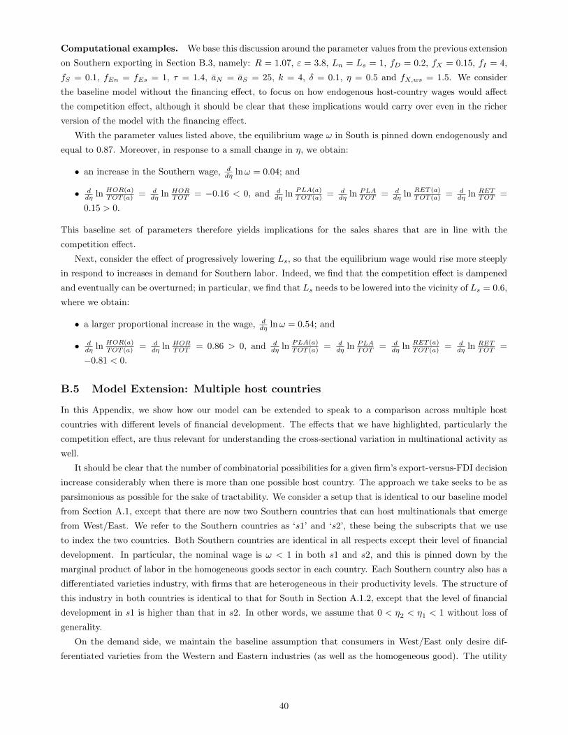
Computational examples. We base this discussion around the parameter values from the previous extension

on Southern exporting in Section B.3, namely: R = 1.07, ε = 3.8, Ln = Ls = 1, fD = 0.2, fX = 0.15, fI = 4,

fS = 0.1, fEn = fEs = 1, τ = 1.4, aN = aS = 25, k = 4, δ = 0.1, η = 0.5 and fX,ws = 1.5. We consider

the baseline model without the financing effect, to focus on how endogenous host-country wages would affect

the competition effect, although it should be clear that these implications would carry over even in the richer

version of the model with the financing effect.

With the parameter values listed above, the equilibrium wage ω in South is pinned down endogenously and

equal to 0.87. Moreover, in response to a small change in η, we obtain:

• an increase in the Southern wage, ddη lnω = 0.04; and

• ddη ln HOR(a)

TOT (a) = ddη ln HOR

TOT = −0.16 < 0, and ddη ln PLA(a)

TOT (a) = ddη ln PLA

TOT = ddη ln RET (a)

TOT (a) = ddη ln RET

TOT =

0.15 > 0.

This baseline set of parameters therefore yields implications for the sales shares that are in line with the

competition effect.

Next, consider the effect of progressively lowering Ls, so that the equilibrium wage would rise more steeply

in respond to increases in demand for Southern labor. Indeed, we find that the competition effect is dampened

and eventually can be overturned; in particular, we find that Ls needs to be lowered into the vicinity of Ls = 0.6,

where we obtain:

• a larger proportional increase in the wage, ddη lnω = 0.54; and

• ddη ln HOR(a)

TOT (a) = ddη ln HOR

TOT = 0.86 > 0, and ddη ln PLA(a)

TOT (a) = ddη ln PLA

TOT = ddη ln RET (a)

TOT (a) = ddη ln RET

TOT =

−0.81 < 0.

B.5 Model Extension: Multiple host countries

In this Appendix, we show how our model can be extended to speak to a comparison across multiple host

countries with different levels of financial development. The effects that we have highlighted, particularly the

competition effect, are thus relevant for understanding the cross-sectional variation in multinational activity as

well.

It should be clear that the number of combinatorial possibilities for a given firm’s export-versus-FDI decision

increase considerably when there is more than one possible host country. The approach we take seeks to be as

parsimonious as possible for the sake of tractability. We consider a setup that is identical to our baseline model

from Section A.1, except that there are now two Southern countries that can host multinationals that emerge

from West/East. We refer to the Southern countries as ‘s1’ and ‘s2’, these being the subscripts that we use

to index the two countries. Both Southern countries are identical in all respects except their level of financial

development. In particular, the nominal wage is ω < 1 in both s1 and s2, and this is pinned down by the

marginal product of labor in the homogeneous goods sector in each country. Each Southern country also has a

differentiated varieties industry, with firms that are heterogeneous in their productivity levels. The structure of

this industry in both countries is identical to that for South in Section A.1.2, except that the level of financial

development in s1 is higher than that in s2. In other words, we assume that 0 < η2 < η1 < 1 without loss of

generality.

On the demand side, we maintain the baseline assumption that consumers in West/East only desire dif-

ferentiated varieties from the Western and Eastern industries (as well as the homogeneous good). The utility

40

function for consumers from n = w, e is thus given once again by:

Un = y1−µn

∑j∈e,w

∫Ωnj

xnj(a)α dGj(a)

µα

, (B.84)

where 0 < α, µ < 1. On the other hand, consumers in each Southern country derive utility from West-

ern/Eastern varieties, as well as from the varieties of their respective domestic industries; for simplicity, they

do not consume the varieties made by the other Southern country. In other words, utility in each si, where

i = 1, 2, is given by:

Usi = y1−µsi

∑j∈e,w,si

∫Ωsi,j

xsi,j(a)α dGj(a)

µα

. (B.85)

Solving the standard utility maximization problem then implies the following expressions for the aggregate

market demand levels:

Aww = Aee = Aew = Awe =µLn

P 1−εww + P 1−ε

we

, and (B.86)

Asi,w = Asi,e = Asi,si =µωLs

P 1−εsi,si + 2P 1−ε

si,w

. (B.87)

Note that Asi,si is now the demand level in country si for its domestic differentiated varieties, while Asi,w and

Asi,e are the corresponding demand levels for the varieties from West and East respectively. From (B.87), these

are functions in particular of the ideal price indices for country-si varieties consumed domestically, Psi,si, and

for Western/Eastern varieties consumed in si, Psi,w.

We examine first the equilibria in the two Southern differentiated varieties industries. Following the industry

structure from our baseline model, the productivity cutoff for domestic entry in each Southern country, which

we denote by a1−εSi for i = 1, 2, is given by:

a1−εSi =

1

ηi

RfSω

(1− α)Asi,si(ω/α)1−ε . (B.88)

Analogously, we can write down the free entry condition in each country si (i = 1, 2) as:

fEsω =1

δ

[(1− α)Asi,si

(ωα

)1−εVs(aS,i)−RfSωGs(aS,i)

]. (B.89)

Inspecting (B.88) and (B.89), it follows as a quick corollary of Lemma 1 that when η1 > η2, we must have

As1,s1 < As2,s2. This is intuitive since ceteris paribus, the country with the higher level of financial development

would facilitate more entry by local firms, so that the aggregate demand level faced by each firm would be lower.

From (B.87), we thus have: As1,w < As2,w.

We turn next to the differentiated varieties sector in West/East. In keeping with the spirit of our baseline

model, we focus on situations in which if a firm from West (likewise East) decides to undertake FDI in either

one of the Southern countries, then that Southern facility will be used as the global production center for that

firm from which all four markets will be serviced, including the other Southern country. (In particular, we

assume that the fixed cost of FDI, fI , is sufficiently large so that the multinational will never seek to establish

more than one foreign affiliate.)

For ease of exposition, we adopt the perspective of a firm headquartered in West; the situation for a firm

from East is entirely symmetric. Suppose that this firm has productivity 1/a. If this Western firm undertakes

41

FDI in host country si, where i ∈ 1, 2, then the horizontal, platform and return sales of its affiliate in si are

given explicitly by:

HORsi(a) = Asi,w (aω/α)1−ε

, (B.90)

PLAsi(a) = (Ae,w +Asj,w) (τaω/α)1−ε

, and (B.91)

RETsi(a) = Aw,w (τaω/α)1−ε

, (B.92)

where j ∈ 1, 2 and j 6= i. (In other words, we use the subscript ‘sj’ to refer to variables relevant to the

Southern country where the firm does not undertake FDI.) From (B.97)-(B.99), the corresponding destination-

specific shares out of total sales are therefore:

HORsi(a)

TOTsi(a)=

(1 +

τ1−ε(Aww +Ae,w +Asj,w)

Asi,w

)−1

, (B.93)

PLAsi(a)

TOTsi(a)=

(1 +

Asi,w + τ1−εAw,wτ1−ε(Ae,w +Asj,w)

)−1

, and (B.94)

RETsi(a)

TOTsi(a)=

(1 +

Asi,w + τ1−ε(Ae,w +Asj,w)

τ1−εAw,w

)−1

. (B.95)

(Note that: TOTsi(a) = HORsi(a) + PLAsi(a) + RETsi(a).) Observe that these sales shares are identical

across all firms, as they do not depend on a. Hence, the expressions in (B.93)-(B.95) are also equal to the

horizontal, platform and return sales shares aggregating across all multinational affiliates from West that are

present in country si.

We now make use of the fact that As1,w < As2,w when η1 > η2. Also, bear in mind that each firm from West

takes the aggregate demand levels, Aw,w, Ae,w, As1,w and As2,w, as given. In particular, these demand levels are

unaffected by the decision of the firm to undertake FDI in either s1 or s2. Applying some straightforward algebra

on (B.93)-(B.95), it immediately follows that: HORs1(a)TOTs1(a) < HORs2(a)

TOTs2(a) , RETs1(a)TOTs1(a) > RETs2(a)

TOTs2(a) and PLAs1(a)TOTs1(a) >

PLAs2(a)TOTs2(a) . In words, we recover the essence of the competition effect in a cross-country comparison across host

countries. Where financial development is higher, the local market is a more competitive environment, so that

the share of horizontal sales is lower, while the return and platform sales shares are higher. With this multiple

host country setup, the implications of host-country financial development for the sales shares of MNC affiliates

thus continue to hold in the cross-section. (Incidentally, in this extension, we also break the symmetry in the

magnitudes of the return and platform sales shares, since platform sales would also include sales to the other

Southern country.)

We now turn to the task of comparing affiliate and aggregate sales levels across the different host countries.

As mentioned in Section A.4.4, this requires that we introduce more structure to the model: For the affiliate-

level comparison to be one that “holds all else constant”, the model should allow for different multinationals

with the same productivity level 1/a to potentially choose to locate in either s1 or s2. There are various

modeling strategies for achieving this, and we present one such possibility here based on allowing for idiosyncratic

realizations of profit shocks from locating in each respective host country.

Consider first an initial setting in which MNCs do not require host-country financing. Western firms that

are contemplating FDI now face both a systematic and a stochastic component to the profits they will earn

from locating in either host country. The systematic component is known in advance, and is equal to their sales

less variable and fixed costs from basing production in the host country in question. However, there is now an

additive stochastic component to these profits, denoted by νs1 and νs2 in the respective host countries; one

can view these as firm-specific idiosyncratic costs that are ex-ante uncertain, the precise values of which are

42

only revealed after the firm has made a decision to pursue FDI. To be clear on the timing of events, a Western

firm first obtains its productivity draw 1/a, on the basis of which it makes an irreversible decision whether or

not to become a multinational. If it should choose to pursue FDI, it then observes the stochastic draws of νs1

and νs2, from which it decides which of s1 or s2 to locate its affiliate in. Firms that choose not to engage in

FDI can either exit, remain purely domestic, or service the foreign markets through exporting, although for the

purposes of this extension, the details of these options are less important.19

For a firm that chooses FDI, the realized profits from locating its production affiliate in s1 and s2 are given

respectively by:

πI,s1(a) = (1− α)(As1,w + τ1−ε(Aw,w +Ae,w +As2,w)

) (aωα

)1−ε−RfI + νs1

πI,s2(a) = (1− α)(As2,w + τ1−ε(Aw,w +Ae,w +As1,w)

) (aωα

)1−ε−RfI + νs2.

In the above, we specify νs1 and νs2 to be iid shocks drawn from a standard Gumbel distribution. Using the

well known properties of the extreme-value distribution, some simple algebra leads to the following expression

for the probability, ps1, that πI,s1(a) > πI,s2(a) and hence that s1 will be chosen as the host country:

ps1 =exp(1− α)

(As1,w + τ1−εAs2,w

)(aω/α)

1−εexp(1− α) (As1,w + τ1−εAs2,w) (aω/α)

1−ε+ exp(1− α) (As2,w + τ1−εAs1,w) (aω/α)1−ε

. (B.96)

Since As1,w < As2,w, we can deduce that As1,w + τ1−εAs2,w < As2,w + τ1−εAs1,w, and hence that ps1 < 1−ps1.

There is thus a larger probability that the profits from locating in s2 will exceed the profits from locating in

s1, since s1 features a more competitive goods market by virtue of its higher level of financial development.

By the law of large numbers, a fraction ps1 (respectively, ps2 ≡ 1 − ps1) of Western firms with productivity

1/a will choose s1 (respectively, s2) as their host country. In turn, a Western firm with productivity 1/a

will choose to become a multinational if it finds that its expected profits from undertaking FDI, given by

E[maxπI,s1(a), πI,s2(a)], exceed that from instead retaining production at home and exporting from there to

all the other foreign markets. Note that the preceding expectation will have to be evaluated over the distribution

of the iid profit shocks, νs1 and νs2. We do not work out this expectation explicitly, as it suffices for our purposes

that this will yield a unique cutoff value which we call aI,twoS .20 In other words, the most productive Western

firms, with a productivity draw 1/a > 1/aI,twoS , will then venture into FDI, and will decide on either s1 or s2

for their host country after observing their realizations of νs1 and νs2.

We now compare the sales levels of two distinct affiliates with the same productivity 1/a that are nevertheless

located in different host countries. From equations (B.90)-(B.92), and the fact that As1,w < As2,w, it follows

immediately that: HORs1(a) < HORs2(a), PLAs1(a) > PLAs2(a) and RETs1(a) = RETs2(a). At the affiliate

level, we therefore recover the implication that the horizontal sales level will be lower and the platform sales

level higher in the host country where financial conditions are better. (Admittedly, the mapping of predictions

into the cross-section is not perfect, as we now have that the level of return sales to West would be identical

for the affiliates in the two host countries.)

The extra structure of the distributional assumption on the νsi’s further allows us to compare the sales

levels aggregated across multinational affiliates in the two host countries. Based on our discussion above, the

measure of affiliates in country si (i = 1, 2) is given precisely by: psiNnGn(aI,twoS). We can also write down

19The irreversibility of the FDI decision could be justified if there were a component of νs1 and νs2 that needs to be incurred asa cost when these stochastic shocks are first observed. For example, one could think of the νsi’s as a learning cost to discover one’strue profitability in each host country, and that a part of these costs becomes sunk once the realizations of νs1 and νs2 are learnt.

20To be fully precise, aI,twoS will be pinned down in conjunction with a free-entry condition for West.

43

the aggregate levels of horizontal, platform and return sales in each si as:

HORsi = psiAsi,w (ω/α)1−ε

Vn(aI,twoS), (B.97)

PLAsi = psi(Ae,w +Asj,w) (τω/α)1−ε

Vn(aI,twoS), and (B.98)

RETsi = psiAw,w (τω/α)1−ε

Vn(aI,twoS), (B.99)

Since ps1 < ps2, we immediately have that the measure of affiliates is lower in the more financially-developed

host, s1. Moreover, from (B.92), it is clear that RETs1 < RETs2. Next, using the additional fact that

As1,w < As2,w, we have from (B.90) that HORs1 < HORs2. Finally, to compare PLAs1 and PLAs2, observe

from (B.96) that:

ps1ps2

=exp(1− α)

(As1,w + τ1−εAs2,w

)(aω/α)

1−εexp(1− α) (As2,w + τ1−εAs1,w) (aω/α)

1−ε=

exp(1− α)As1,w(1− τ1−ε) (aω/α)1−ε

exp(1− α)As2,w(1− τ1−ε) (aω/α)1−ε

<As1,wAs2,w

,

where the last inequality comes from applying the fact that: (i) expx/x is an increasing function in x for

all x > 1; and (ii) As1,w < As2,w. (Note that we need to ensure through a suitable normalization that (1 −α)(As1,w + τ1−εAs2,w

)(aω/α)

1−εand (1− α)

(As2,w + τ1−εAs1,w

)(aω/α)

1−εboth exceed 1, so that property

(i) can be applied. This can be achieved by assuming that the labor endowment in each host country is

sufficiently big.) From the above, we have that: ps1As2,w < ps2As1,w, which together with (B.91) implies that

PLAs1 < PLAs2. In sum, we find that comparing the two FDI hosts, the country with the higher level of

financial development features fewer affiliates and lower aggregate sales levels; this provides the analogue to

part (iii) of Proposition 1.

Last but not least, we briefly discuss the case where multinationals require host country financing. Observe

that the expressions for the sales shares in (B.93)-(B.95) and for the sales levels of individual affiliates in (B.90)-

(B.92) remain valid even when MNCs seek local financing, as long as the affiliates being compared are both able

to secure this financing from the respective host country institutions. The same arguments as above can then

be applied to show that s1 will still be a more competitive market environment than s2, so that As1,w < As2,w.

One can then quickly see that the following comparisons still hold: HORs1(a)TOTs1(a) <

HORs2(a)TOTs2(a) , RETs1(a)

TOTs1(a) >RETs2(a)TOTs2(a) ,

PLAs1(a)TOTs1(a) >

PLAs2(a)TOTs2(a) and HORs1(a) < HORs2(a). These cross-sectional implications are consistent with parts

(i) and (ii) of Proposition 2.

With host-country financing, the analysis for aggregate measures of multinational activity is in general

more complicated in terms of the cases that would need to be enumerated. For example, it is possible that

some prospective multinationals would be productive enough to receive funding in country s1, but not in s2.

However, a clear comparison can nevertheless be made in the limiting case where η2 −→ 0. In this situation,

the cost of default would approach zero in s2. In the limit, there would therefore be no affiliates in s2, although

there would be a positive measure in s1. The number of multinational affiliates, as well as the aggregate levels

of horizontal, platform and return sales, would clearly be higher in the more financially-developed host country

s1 than in s2. In sum, when host-country financing is required, the qualitative prediction that the aggregate

level of multinational activity would be higher in s1 is preserved when financial development in s2 is sufficiently

low.

44