Hopf bifurcation control in the XCP for the Internet congestion control system

Nonlinear Analysis: Real World Applications 13 (2012) 1466–1479

Contents lists available at SciVerse ScienceDirect

Nonlinear Analysis: Real World Applications

journal homepage: www.elsevier.com/locate/nonrwa

Hopf bifurcation control in the XCP for the Internet congestioncontrol systemFeng Liu a,b,c, Hua O. Wang b, Zhi-Hong Guan c,∗

a Department of Electronic Information and Mechanics, China University of Geosciences, Wuhan 430074, Chinab Department of Mechanical Engineering, Boston University, Boston, MA 02215, USAc Department of Control Science and Engineering, Huazhong University of Science and Technology, Wuhan 430074, China

a r t i c l e i n f o

Article history:Received 12 April 2011Accepted 16 November 2011

Keywords:XCP systemHopf bifurcationBifurcation control

a b s t r a c t

In this paper, we investigated the Hopf bifurcation of the eXplicit Control Protocol(XCP) for the Internet congestion control system. These bifurcation behaviors may causeheavy oscillation of average queue length and induce network instability. A time-delayedfeedback control method was proposed for controlling Hopf bifurcation in the XCP system.Numerical simulation results are presented to show that the time-delayed feedbackcontroller is efficient in controlling Hopf bifurcation.

© 2011 Elsevier Ltd. All rights reserved.

1. Introduction

With an increasing number and variety of Internet applications, Internet congestion occurswhen the aggregated demandfor a resource exceeds the available capacity of the resource and the routers in the network receive more packets than theycan forward, which can cause dropping packets and increasing delays, the upper formation application system performancedrop, and can even break the whole system by causing congestion collapse. If the congestion control scheme is not welldesigned, the sources will try to push even more packets through the network in response to packet drops, thus worseningthe congestion [1]. The aim of congestion control is to regulate the sending rates of the sources such that high networkutilization, small amounts of queuing delay, and some degree of fairness among users are obtained. Over the past decade,congestion control in the Internet is an extremely important and challenging problem, which has been the main subject ofintensive studies. The research of network congestion control becomes a key issue.

The stability of the Internet is largely dependent on the congestion control and avoidance mechanisms implementedin its end-to-end transmission control protocol (TCP), developed by Jacobson in 1980s [1]. However, this implementingfrom the network edge control mechanism is extremely limited, it is not sufficient to provide good services with only theTCP congestion control on the Internet in all circumstances. Therefore, the network expert suggested using the strategy ofActive Queue Management (AQM) [2] in network routers. Active Queue Management (AQM) interacts with TCP congestioncontrol mechanisms [3], which plays an important role in meeting today’s increasing demand for quality of service.

There has beenmuch interest recently in fluid-flowmodels to analyze the stability of congestion control protocols [4–6].It has been observed that the congestion control algorithm TCP [2] is prone to instability as the bandwidth-delay product ofthe network grows [6,7]. Recently, some new congestion control algorithms, such as the eXplicit Control Protocol (XCP) [7]and the Rate Control Protocol (RCP) [8], have been proposed as modifications to TCP (such as HSTCP [9], FAST [10], andSTCP [11]).

∗ Corresponding author.E-mail addresses: [email protected] (F. Liu), [email protected] (Z.-H. Guan).

1468-1218/$ – see front matter© 2011 Elsevier Ltd. All rights reserved.doi:10.1016/j.nonrwa.2011.11.010

http://dx.doi.org/10.1016/j.nonrwa.2011.11.010

http://www.elsevier.com/locate/nonrwa

http://www.elsevier.com/locate/nonrwa

mailto:[email protected]

mailto:[email protected]

http://dx.doi.org/10.1016/j.nonrwa.2011.11.010

F. Liu et al. / Nonlinear Analysis: Real World Applications 13 (2012) 1466–1479 1467

Analysis and control of nonlinear dynamical models in Internet congestion control system have attracted manyresearchers in recent years. The nonlinear dynamics of congestion control system motivates researchers to improve theperformance of AQM schemes by existing bifurcation control methods. Subsequently, there have been many papers whichhave addressed nonlinear behavior such as bifurcation and chaos in models of network systems [12–44].

The rest of this paper is organized as follows. In Section 2, the linear stability and Hopf bifurcation analysis are studiedfor an XCP model. Section 3 is devoted to the direction and stability analysis of the Hopf bifurcation on normal form theoryand center manifold approach on time-delayed feedback controlled XCP system. Numerical simulations are given to verifythe theoretical results in Section 4. Finally conclusion is given in Section 5.

2. Linear stability and Hopf bifurcation analysis

For a single bottleneck link of capacity C traversed by N flows with equal round trip delays d, aggregate flow rate y(t),and queue length q(t), the system can be modeled by the following delay differential equations [7]

y(t) = −α

d(y(t − d)− C)−

β

d2q(t − d)

q(t) =

y(t)− C, q(t) > 0max [0, y(t)− C] , q(t) = 0

(1)

where q is the queue size and y is the aggregate traffic rate.

2.1. Linear stability analysis

We defined x(t) = y(t) − C for system (1). Substituting it into the differential equation (1), we obtain the followinglinearized equations:

x(t) = −α

dx(t − d)−

β

d2q(t − d), q > 0 or x ≥ 0

q(t) = x(t).(2)

The equilibrium point (x∗, q∗) of system (2) is given by

x∗= 0, q∗

= 0. (3)

Then the characteristic equation of system (2) is

λ2 +α

dλe−λd

+β

d2e−λd

= 0. (4)

Under the quadratic approximation e−λd≈ 1 − λd + λ2d2/2, the above equation becomes

αd2λ3 +

1 − α +

β

2

λ2 +

α − β

d

λ+

β

d2= 0. (5)

The system described by (2) is stable if and only if all the roots of the characteristic Eq. (5) are in the open left-half plane.Routh–Hurwitz stability criterion states that the closed-loop system is stable if and only if the values of the Routh table ofthe second column are all greater than zero, i.e., if it satisfies the following conditions,

αd2> 0,

1 − α +

β

2

> 0,

α − β + αβ − α2

−β2

2

> 0,

β

d2> 0 (6)

the XCP system (2) is considered to be stable.

2.2. Hopf bifurcation analysis

The characteristic equation of system (2) is

λ2 + ae−λdλ+ be−λd= 0 (7)

where a =αd > 0, b =

β

d2> 0.

For d > 0, let λ = ±iω,ω > 0. Then substituting λ = iω in Eq. (7) yieldsb − ω2 cosωd = 0aω − ω2 sinωd = 0.

(8)

1468 F. Liu et al. / Nonlinear Analysis: Real World Applications 13 (2012) 1466–1479

For ω > 0, from Eq. (8) we obtain,ω0 =

(a2 +

a4 + 4b2)/2

a0 = ω0 sin(ω0d).(9)

In order to conduct a Hopf bifurcation analysis we choose a parameter which induces the bifurcation. We consider α asthe bifurcation parameter of (2). As this parameter varies, it induces a Hopf bifurcation. Thus it follows from the coefficientsin Eqs. (7) and (9) that

α = ω0d sin(ω0d) (10)

where αc denotes the critical value of α at ω = ω0.Next we prove that λ = ±iω0 are simple roots of Eq. (7) when α = αc . Now defining

∆(λ, α) = eλdλ2 + (α/d)λ+ b (11)

we have

d∆(λ, α)dλ

= 2λeλd + (α/d)+ λ2deλd. (12)

Substituting λ = iω0 into (12), we get

d∆(λ, α)dλ

λ=iω0

= −2ω0 sinω0d + (α/d)− ω20 cosω0d + i(−ω2

0d sinω0d + 2ω0 cosω0d) = 0. (13)

Similarly, we obtain d∆(λ,α)dλ |λ=−iω0 = 0. Hence we get the following lemma.

Lemma 1. When α = αc , Eq. (7) has a pair of purely imaginary roots λ = ±iω0 which are simple.

We also need to satisfy the transversality condition of the Hopf spectrum.

Lemma 2. Let λ(α) = R(α)+ iω(α) be the root of Eq. (7) satisfying R(αc) = 0, ω(αc) = ω0, then

Redλ(α)dα

α=αc

> 0.

Proof. Differentiating Eq. (7) on α and applying the implicit function theorem, we obtain

dλdα

α=αc

=−λ

2λdeλd + α − αλd − β

α=αc

. (14)

Then dλdα

α=αc

−1

= αd − 2deλd + (β − α)/λ

= αd − 2deRd cosω0d + (β − α)R/(R2+ ω2

0)+ i−2deRd sinω0d − (β − α)ω0/

R2

+ ω20

dReλ(α)

dα

α=αc

−1

= αcd − 2deRd cosω0d + (β − αc) R/R2

+ ω20

.

(15)

From Eq. (8), we know 0 < ω0d < π/2.As we know, when d > 0, α > 0, 0 < cosω0d < 1, R(αc) = 0. Therefore, we obtain

Redλ(α)dα

α=αc

> 0. � (16)

From Lemma 2, and by using the lemma in [45], we can obtain the following lemma.

Lemma 3. When α > αc , Eq. (7) has at least one root with a strictly positive real part.

Based on the above lemmas, we obtain the following bifurcation theorem for Eq. (2) by applying the Hopf bifurcationtheorem [46–49] for delayed differential equations [50].


Theorem 1. For system (2), the following results hold.

(1) When α < αc , the equilibrium point is locally asymptotically stable.(2) When α > αc , the equilibrium point is unstable.(3) When α = αc , system (2) exhibits a Hopf bifurcation.

Remark 1. We know that system (2) is equivalent to the system (1). Theorem 1 shows that one can change the state of theoriginal equilibrium points by choosing an appropriate value of α. When the parameter α is smaller than the critical valueαc = ω0d sin(ω0d) the equilibrium point of system (1) is asymptotically stable. When the parameter α passes through αc ,there is a Hopf bifurcation of system (1) at its equilibrium point. When the parameter α is larger than the critical value αcthe equilibrium point of system (1) is unstable.

3. Hopf bifurcation control

In this section, we design a time-delayed feedback controller to the original model for controlling the Hopf bifurcationin XCP system. Following the idea of polynomial function controller [23], we get the following time-delayed feedbackcontrolled modelx(t) = −

α

dx(t − d)−

β

d2q(t − d)+ a1(x(t − d)− x∗)+ a2(x(t − d)− x∗)2 + a3(x(t − d)− x∗)3,

q(t) = x(t),(17)

where x∗ is the equilibrium point of system (2). a1, a2 and a3 are parameters, which can control the Hopf bifurcation todesired behaviors.

Using Taylor expansion to expand the right hand side of Eq. (17) at the equilibrium point, we havey1(t) = a11y1(t − d)+ a12y2(t − d)+ a13y21(t − d)+ a14y31(t − d),y2(t) = a21y1(t),

(18)

where a11 = a1 −αd , a12 = −

β

d2, a13 = a2, a14 = a3, a21 = 1.

From the linearized equation of (18), we havey1(t) = a11y1(t − d)+ a12y2(t − d),y2(t) = a21y1(t).

It is observed that the above equation is similar to Eq. (2). As the analysis method is similar to Section 2, we omit the linearstability and Hopf bifurcation analysis of Eq. (18).

In the following, we use the normal form and the center manifold theorem [46] to study the direction of Hopf bifurcationand the stability of bifurcating periodic solution of (18) at equilibrium when α passes through certain critical values.

Let α = α∗+ µ, u(t) = (y1(t), y2(t))T and ut(θ) = u(t + θ) for θ ∈ [−d, 0]. Then µ = 0 is a Hopf bifurcation value for

Eq. (2). For initial condition ϕ(θ) = (ϕ1(θ), ϕ2(θ))T

∈ C[−d, 0], we rewrite Eq. (18) as

u(t) = Lµut + F(ut , µ) (19)

with

Lµϕ = B1ϕ(0)+ B2ϕ(−d) (20)

and

F(ϕ, µ) =

a13ϕ2

1(t − d)+ a14ϕ31(t − d)

0

,

where Lµ is one parameter family of bounded linear operator in C [−d, 0] and

B1 =

0 0a21 0

, B2 =

a11 a120 0

.

By the Riesz representation theorem, there exists a 2 × 2 matrix-valued function

η(·, µ): [−d, 0] → R2×2

for ϕ ∈ C [−d, 0], such that

Lµϕ =

∫ 0

−ddη(θ, µ)ϕ(θ) (21)


where

η(θ, µ) = B1δ(θ)+ B2δ(θ + d), θ ∈ C[−d, 0] (22)

where δ(θ) is the Dirac delta function.For ϕ ∈ C [−d, 0], we define

A(µ)ϕ =

dϕdθ, θ ∈ [−d, 0),∫ 0

−ddη(θ, µ)ϕ(θ) = Lµϕ, θ = 0,

(23)

and

R(µ)ϕ =

0, θ ∈ [−d, 0),F(µ, ϕ), θ = 0.

Since dut/dθ = dut/dt , Eq. (19) can be rewritten as

ut = A(µ)ut + R(µ)ut (24)

where ut = u(t + θ) for θ ∈ [−d, 0).The bifurcation periodic solutions u(t, µ(ε)) of (17) (where ε ≥ 0 is a small parameter) have period T (ε) and a nonzero

Floquet exponent β(ε), where µ, T and β have the following expansions:

µ = µ2ε2+ µ4ε

4+ · · · ,

T =2πω0(1 + T2ε2 + T4ε4 + · · ·),

β = β2ε2+ β4ε

4+ · · · .

The sign of µ2 determines the direction of bifurcation while that of β2 determines the stability of u(t, µ(ε)). We onlyneed to compute the coefficients in these expansions at µ = 0.

For ψ ∈ C[0, d], the adjoint operator A∗ of A is defined as

A∗ψ(s) =

−

dψ(s)ds

, s ∈ (0, d],∫ 0

−ddηT (t, 0)ψ(−t), s = 0.

(25)

For ϕ ∈ C[−d, 0] and ψ ∈ C[0, d], we define a bilinear form by

⟨ψ, ϕ⟩ = ψT (0)ϕ(0)−

∫ 0

θ=−d

∫ θ

ξ=0ψT (ξ − θ) [dη(θ)]ϕ(ξ)dξ, (26)

where η(θ) = η(θ, 0).From the above analysis, we know that ±iω0 are the eigenvalues of A and A∗. Let q(θ) be the eigenvector of A associated

with eigenvalue iω0 and the eigenvector q∗(θ) of A∗ associated with eigenvalue −iω0. Then we have the following lemma.

Lemma 4. Let q(θ) = Deiω0θ be the eigenvector of A associated with eigenvalue iω0 and the eigenvector q∗(θ) = DV ∗eiω0θ bethe eigenvector of A∗ associated with eigenvalue −iω0. Then

q∗, q= 1,

q∗, q

= 0

where

V = (1, ρ1)T , ρ1 = a21/iω0

V ∗= (ρ2, 1)T , ρ2 = (iω0a11 − a12a21)/iω0a12

D =

V ∗

TV + d0e−iω0dV ∗

TB2V

−1.

Proof. Suppose q(θ) be the eigenvector of A(0) associatedwith iω0 and q∗(θ) the eigenvector of A∗(0) associatedwith−iω0.Then we have

A(0)q(θ) = iω0q(θ), A∗(0)q(θ) = −iω0q∗(θ). (27)


From (23), we can rewrite (27) asdq(θ)dθ

= iω0q(θ), θ ∈ [−d, 0),

L(0)q(0) = iω0q(0), θ = 0.(28)

Therefore, we can obtain

q(θ) = Veiω0θ , θ ∈ [−d, 0],

where V = (v1, v2)T

∈ C2 is a constant vector. Based on (20) and (28), we haveB1 − iω0I + B2e−iω0d

V = 0,

where I is identity matrix.Therefore

a11e−iω0d − iω0 a12e−iω0d

a21 −iω0

v1v2

= 0.

So, we can choose

V =

v1v2

=

1ρ1

=

1

a21/iω0

.

From (28), we can obtain

A∗ψ =

∫ 0

−ddηT (t, 0)ψ(−t) = BT

1ψ(0)+ BT2ψ(d).

Let

q∗(θ) = DV ∗eiω0θ , θ ∈ [0, d],

where D = (d1, d2)T , V ∗= (v∗

1 , v∗

2)T

∈ C2 are constant vectors.Similarly, we can get

V ∗=

v∗

1v∗

2

=

ρ21

=

(iω0a11 − a12a21)/iω0a12

1

.

Then we calculate the parameter B and normalize q and q∗ by the condition ⟨q∗, q⟩ = 1. From (26), we obtainq∗, q

= q∗

Tq(0)−

∫ 0

−d

∫ θ

ξ=0q∗

T(ξ − θ) [dη(θ)] q(ξ)dξ

= D[V ∗

TV −

∫ 0

−d

∫ θ

ξ=0V ∗

Te−iω0(ξ−θ)[dη(θ)]Veiω0ξdξ

]= D

[V ∗

TV −

∫ 0

−dV ∗

T[dη(θ)]eiω0θV

]= D

V ∗

TV + de−iω0dV ∗

TB2V

. (29)

So, let D =

V ∗

TV + de−iω0dV ∗

TB2V

−1, we can obtain ⟨q∗, q⟩ = 1.

Since ⟨ψ, Aϕ⟩ = ⟨A∗ψ, ϕ⟩, we have

−iω0q∗, q

=

q∗, Aq

=

A∗q∗, q

=

−iω0q∗, q

= iω0

q∗, q

.

Therefore ⟨q∗, q⟩ = 0. This completes the proof. �

Let ut be solution of Eq. (24) at µ = 0, we define

z =q∗, ut

and

w(t, θ) = ut − zq − zq = ut − 2 Re {z(t)q(θ)} . (30)

On the manifold C0, we have

w(t, θ) = w(z(t), z(t), θ),


where

w(z, z, θ) = w20(θ)12z2 + w11(θ)zz + w02(θ)

12z2 + · · · (31)

where z and z are local coordinates of center manifold C0 in the direction of q∗ and q∗. Note that w is real if ut is real. Weconsider only real solutions. From (30), it is easy to get

q∗, w=

q∗, ut − zq − zq

=

q∗, ut

− z(t)

q∗, q

− z(t)

q∗, q

= 0.

For solutions ut ∈ C0 of (24), from (23) and (30), since µ = 0, we have

z(t) =q∗, ut

=

q∗, A(0)ut + R(0)ut

=

A∗q∗, ut

+ q∗

T(0)F(ut , 0)

= iω0z(t)+ q∗T(0)f0(z, z)

which we can rewrite in abbreviated form as

z(t) = iω0z(t)+ g(z, z) (32)

where

g(z, z) = q∗T(0)f0(z, z)

= q∗T(0)F (w(z, z, θ)+ 2Re {z(t)q(θ)} , 0)

=12g20z2 + g11zz +

12g02z2 +

12g21z2z + · · · . (33)

By (24) and (32), we have

w = ut − zq − ˙zq

= Aut + Rut − iω0zq − q∗T(0)f0(z, z)q + iω0zq − q∗

T(0)f0(z, z)q

= Aut + Rut − Azq − Azq − 2Req∗

T(0)f0(z, z)q

= Aut + Rut − 2Re

q∗

T(0)f0(z, z)q

=

Aw − 2Re

q∗

T(0)f0(z, z)q

, θ ∈ [−d, 0),

Aw − 2Req∗

T(0)f0(z, z)q

+ f0(z, z), θ = 0.

(34)

We can rewrite (34) as

w = Aw + H(z, z, θ), (35)

where

H(z, z, θ) =12H20(θ)z2 + H11(θ)zz +

12H02(θ)z2 + · · · . (36)

On the other hand, on C0

w = wz z + wz ˙z. (37)

Substituting (31) and (32) into (37), we obtain

w = iω0w20(θ)z2 − iω0w02z2 + · · · .

Comparing the coefficients of the above equation with those of Eq. (35), we have

(A − i2ω0) w20(θ) = −H20(θ), Aw11(θ) = −H11(θ), (A + i2ω0) w02(θ) = −H02(θ). (38)

Since ut = u(t + θ) = w(z, z, θ)+ zq + zq, we have

ut =

y1 (t + θ)y2 (t + θ)

=

w(1)(z, z, θ)w(2)(z, z, θ)

+ z

1ρ1

eiω0θ + z

1ρ1

e−iω0θ .


Therefore, we can obtain

y1(t + θ) = w(1)(z, z, θ)+ zeiω0θ + ze−iω0θ

= zeiω0θ + ze−iω0θ +12w(1)20 (θ)z

2+ w

(1)11 (θ)zz +

12w(1)02 (θ)z

2+ · · ·

and

y2(t + θ) = w(2)(z, z, θ)+ zρ1eiω0θ + zρ1e−iω0θ

= zρ1eiω0θ + zρ1e−iω0θ +12w(2)20 (θ)z

2+ w

(2)11 (θ)zz +

12w(2)02 (θ)z

2+ · · · .

Therefore, we have

ϕ1(−d) = ze−iω0d + zeiω0d +12w(1)20 (−d)z2 + w

(1)11 (−d)zz +

12w(1)02 (−d)z2 + · · · ,

ϕ21(−d) = e−i2ω0dz2 + 2zz + ei2ω0dz2 +

eiω0dw

(1)20 (−d)+ 2e−iω0dw

(1)11 (−d)

z2z + · · · ,

ϕ31(−d) = 3e−iω0dz2z + · · · .

Then we have

f (z, z) =

a13ϕ2

1(t − d)+ a14ϕ31(t − d)

0

=

K1z2 + K2zz + K3z2 + K4z2z + · · ·

0

,

where

K1 = a13e−i2ω0d,

K2 = 2a13,K3 = a13ei2ω0d,

K4 = a132e−iω0dw

(1)11 (−d)+ eiω0dw

(1)20 (−d)

+ 3a14e−iω0d.

Since q∗(0) = D(ρ2, 1)T , we have

g(z, z) = q∗T(0)f0(z, z)

= D(ρ2, 1)K1z2 + K2zz + K3z2 + K4z2z

0

= Dρ2

K1z2 + K2zz + K3z2 + K4z2z

.

Comparing the coefficients of the above equation with those in (33), we have

g20 = 2Dρ2K1,

g11 = 2Dρ2K2,

g02 = 2Dρ2K3,

g21 = 2Dρ2K4.

(39)

We still need to computew20(θ) andw11(θ) for θ ∈ [−d, 0) for the expression of g21. From (34) to (35), we have

H(z, z, θ) = −2Req∗

T(0)f0(z, z)q(θ)

= −2Re {g(z, z)q(θ)}= −g(z, z)q(θ)− g(z, z)q(θ)

= −

12g20z2 + g11zz +

12g02z2 +

12g21z2z + · · ·

q(θ)

−

12g20z2 + g11zz +

12g02z2 +

12g21z2z + · · ·

q(θ).

Comparing the coefficients of the above equation with those in (36), it is obvious that

H20(θ) = −g20q(θ)− g02q(θ),H11(θ) = −g11q(θ)− g11q(θ).


It follows from (23) to (38) that

w20(θ) = Aw20(θ)

= i2ω0w20(θ)− H20(θ)

= i2ω0w20(θ)+ g20q(θ)+ g02q(θ)= i2ω0w20(θ)+ g20q(0)eiω0θ + g02q(0)e−iω0θ .

Solving forw20(θ), we obtain

w20(θ) = ig20ω0

q(0)eiω0θ + ig023ω0

q(0)e−iω0θ + E1ei2ω0θ . (40)

Similarly, from (38) to (40) we have

w11(θ) = −ig11ω0

q(0)eiω0θ + ig11ω0

q(0)e−iω0θ + E2 (41)

where E1 and E2 are both two-dimensional vectors. They can be determined by setting θ = 0 in H(z, z, θ). It is evident that

H(z, z, 0) = −2Req∗

T(0)f0(z, z)q(0)

+ f0(z, z)

= −

12g20z2 + g11zz +

12g02z2 +

12g21z2z + · · ·

q(0)

−

12g20z2 + g11zz +

12g02z2 +

12g21z2z + · · ·

q(0)+

K1z2 + K2zz + K3z2 + K4z2z

0

.

Comparing the coefficients of the above equation with those in (36), we obtain

H20(0) = −g20q(0)− g02q(0)+

K10

,

H11(0) = −g11q(0)− g11q(0)+

K20

.

By the definition of A and Eq. (38), we can get∫ 0

−ddη(θ)w20(θ) = Aw20(0) = i2ω0w20(0)− H20(0)∫ 0

−ddη(θ)w11(θ) = Aw11(0) = −H11(0).

(42)

Since q(θ) is the eigenvector for A corresponding to iω0, it satisfies∫ 0

−ddη(θ)q(θ) = iω0q(θ)I.

We obtainiω0I −

∫ 0

−deiω0θdη(θ)

q(0) = 0

−iω0I −

∫ 0

−de−iω0θdη(θ)

q(0) = 0.

Thus, we can obtaini2ω0I −

∫ 0

−dei2ω0θdη(θ)

E1 =

K10

∫ 0

−ddη(θ)

E2 = −

K20

where E1 =

E(1)1 E(2)1

T, E2 =

E(1)2 E(2)2

T.

Hence, it follows thati2ω0 − a11e−i2ω0d −a12e−i2ω0d

−a21 i2ω0

E(1)1E(2)1

=

K10

a11 a12a21 0

E(1)2E(2)2

= −

K20

.

(43)


From (43), we can obtain

E(1)1 =i2ω0K1

4ω20 + i2ω0a11e−i2ω0d + a12a21e−i2ω0d

,

E(2)1 =a21i2ω0

E(1)1 ,

(44)

and

E(1)2 = 0,

E(2)2 = −K2

a12.

(45)

Based on the above analysis, we can see that each gij in (39) is determined by parameters and delays in (17). Thus, we cancompute the following quantities:

C1(0) =i

2ω0

g20g11 − 2 |g11|2 −

13

|g02|2

+12g21, (46)

µ2 = −Re {C1(0)}Re {λ′(0)}

,

T2 = −Im {C1(0)} + µ2Im

λ′(α0)

ω0

,

β2 = 2Re {C1(0)}

where

λ′(0) =−a11d2 − 2d cos(ω0d)+ i

2d sin(ω0d)+ (a11d − a12d2)ω−1

0

−a11d2 − 2d cos(ω0d)

2+

2d sin(ω0d)+ (a11d − a12d2)ω−1

0

2 .From the discussion in this section, we have the following result:

Theorem 2. For system (17), when α = α0, the direction and stability of periodic solutions of the Hopf bifurcation is determinedby the formulas (44) and the following results hold.

(1) µ2 determines the direction of the Hopf bifurcation. If µ2 > 0(< 0), the Hopf bifurcation is supercritical (subcritical) andthe bifurcating periodic solutions exist.

(2) β2 determines the stability of the bifurcating periodic solutions. If β2 < 0 (> 0), the bifurcating periodic solutions areorbitally stable (unstable).

(3) T2 determines the period of the bifurcating periodic solutions. If T2 > 0 (< 0), the period increases (decreases).

4. Numerical simulation examples

In this section, we verify our theoretical analysis for the existence of Hopf bifurcation in Sections 2 and 3 and determinethe stability and direction of the bifurcating periodic solutions of system (17) with the parameters of the system as follows

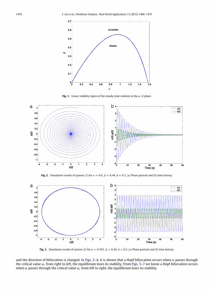
Let d = 0.2s, β = 0.44.From (8), we can plot the linear stability region of the steady state solution in the α–β plane in Fig. 1. From the figure,

we know that if the values α and β are in the region, the steady state solution of the system is stable and a Hopf bifurcationoccurs when the values α and β are a point on the curve.

From the analysis in Section 2, we have

x∗= 0, q∗

= 0, ω0 = 3.9256, αc = 0.555.

By choosing α = 0.54, 0.555 and 0.6, the dynamical behavior of XCP system (2) is illustrated in Figs. 2–4. From these figureswe know when α > αc , the system equilibrium point is asymptotically stable (see Fig. 2), when it is decreased to pass αc ,the system loses stability and a Hopf bifurcation occurs (see Figs. 3 and 4).

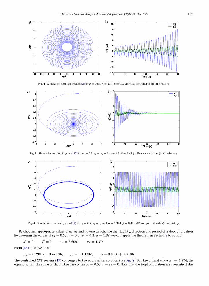
We choose the values of a1 = 0.5, a2 = a3 = 0 to control the Hopf bifurcation. From the analysis in Section 3, we obtain

x∗= 0, q∗

= 0, ω0 = 3.7136, αc = 1.374.

By choosing α = 1.3, 1.374 and 1.38, the dynamical behavior of the controlled XCP system (17) is illustrated in Figs. 5–7.From these figures we know when α < αc , the system equilibrium point is asymptotically stable (see Fig. 5), when it isincreased to pass αc , the system loses stability and a Hopf bifurcation occurs (see Figs. 6 and 7).

Comparing Figs. 2–4 with Figs. 5–7, it shows that the controlled XCP system (17) has the same equilibrium point as thatof the original XCP system (2), the onset of Hopf bifurcation is delayed, the critical value αc increases from 0.555 to 1.374,


ββ

α

Fig. 1. Linear stability region of the steady state solution in the α–β plane.

Fig. 2. Simulation results of system (2) for α = 0.6, β = 0.44, d = 0.2. (a) Phase portrait and (b) time history.


and the direction of bifurcation is changed. In Figs. 2–4, it is shown that a Hopf bifurcation occurs when α passes throughthe critical value αc from right to left, the equilibrium loses its stability. From Figs. 5–7 we know a Hopf bifurcation occurswhen α passes through the critical value αc from left to right, the equilibrium loses its stability.



Fig. 5. Simulation results of system (17) for a1 = 0.5, a2 = a3 = 0, α = 1.3, β = 0.44. (a) Phase portrait and (b) time history.


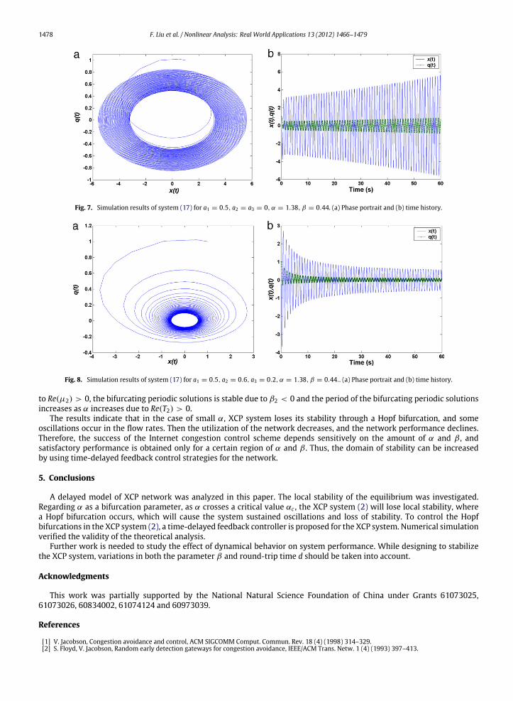
By choosing appropriate values of a1, a2 and a3, one can change the stability, direction and period of a Hopf bifurcation.By choosing the values of a1 = 0.5, a2 = 0.6, a3 = 0.2, α = 1.38, we can apply the theorem in Section 3 to obtain

x∗= 0, q∗

= 0, ω0 = 6.6091, αc = 1.374.

From (46), it shows that

µ2 = 0.29032 − 0.47938i, β2 = −1.1382, T2 = 0.0056 + 0.0630i.

The controlled XCP system (17) converges to the equilibrium solution (see Fig. 8). For the critical value αc = 1.374, theequilibrium is the same as that in the case when a1 = 0.5, a2 = a3 = 0. Note that the Hopf bifurcation is supercritical due



Fig. 8. Simulation results of system (17) for a1 = 0.5, a2 = 0.6, a3 = 0.2, α = 1.38, β = 0.44.. (a) Phase portrait and (b) time history.

to Re(µ2) > 0, the bifurcating periodic solutions is stable due to β2 < 0 and the period of the bifurcating periodic solutionsincreases as α increases due to Re(T2) > 0.

The results indicate that in the case of small α, XCP system loses its stability through a Hopf bifurcation, and someoscillations occur in the flow rates. Then the utilization of the network decreases, and the network performance declines.Therefore, the success of the Internet congestion control scheme depends sensitively on the amount of α and β , andsatisfactory performance is obtained only for a certain region of α and β . Thus, the domain of stability can be increasedby using time-delayed feedback control strategies for the network.

5. Conclusions

A delayed model of XCP network was analyzed in this paper. The local stability of the equilibrium was investigated.Regarding α as a bifurcation parameter, as α crosses a critical value αc , the XCP system (2) will lose local stability, wherea Hopf bifurcation occurs, which will cause the system sustained oscillations and loss of stability. To control the Hopfbifurcations in the XCP system (2), a time-delayed feedback controller is proposed for the XCP system. Numerical simulationverified the validity of the theoretical analysis.

Further work is needed to study the effect of dynamical behavior on system performance. While designing to stabilizethe XCP system, variations in both the parameter β and round-trip time d should be taken into account.

Acknowledgments

This work was partially supported by the National Natural Science Foundation of China under Grants 61073025,61073026, 60834002, 61074124 and 60973039.

References

[1] V. Jacobson, Congestion avoidance and control, ACM SIGCOMM Comput. Commun. Rev. 18 (4) (1998) 314–329.[2] S. Floyd, V. Jacobson, Random early detection gateways for congestion avoidance, IEEE/ACM Trans. Netw. 1 (4) (1993) 397–413.


[3] V. Misra, W.B. Gong, D. Towlsey, Fluid-based analysis of a network of AQM routers supporting TCP flows with an application to RED, Proc. ACMSIGCOMM (2000) 151–160.

[4] J.P. Hepanha, S. Bohacek, K. Obrxzka, J. Lee, Hybrid modeling of TCP congestion control, Lect. Notes Comput. Sci. 2034 (2001) 291–304.[5] C.V. Hollot, V. Misra, D. Towsley, W-B. Gong, A control theoretic analysis of RED, Proc. IEEE INFOCOM (2001).[6] S.H. Low, F. Paganini, J. Wang, S. Adlakha, J.C. Doyle, Dynamics of TCP/RED and a scalable control, Proc. IEEE INFOCOM (2002).[7] D. Katabi, M. Handley, C. Rohrs, Congestion control for high bandwidth-delay product networks, Proc. ACM SIGCOMM (2002).[8] N. Dukkipati, M. Kobayashi, R. Zhang-Shen, N. McKeown, Processor sharing flows in the internet, in: Thirteenth International Workshop on Quality of

Service, 2005.[9] S. Floyd, HighSpeed TCP for large congestion windows, (2003) RFC Editor 3649.

[10] C. Jin, D.X. Wei, S.H. Low, FAST TCP: motivation, architecture, algorithms, performance, Proc. IEEE INFOCOM (2004).[11] T. Kelly, Scalable TCP: improving performance in highspeed wide area networks, Comput. Commun. Rev. 32 (2) (2003).[12] A. Veres, M. Boda, The chaotic nature of TCP congestion control, Proc. IEEE INFOCOM 3 (2000) 1715–1723.[13] L. Massoulie, Stability of distributed congestion control with heterogeneous feedback delays, IEEE Trans. Automat. Control 47 (6) (2002) 895–902.[14] G. Walsh, H. Ye, L. Bushnell, Stability analysis of network control systems, IEEE Control Syst. Technol. 10 (3) (2002) 438–446.[15] F.P. Kelly, Fairness and stability of end-to-end congestion control, Eur. J. Cont. 9 (2003) 149–165.[16] R. Srikant, The Mathematics of Internet Congestion Control, Birkhauser, 2004.[17] P. Ranjan, E.H. Abed, Nonlinear instabilities in TCP-RED, IEEE/ACM Trans. Netw. 12 (6) (2004) 1079–1092.[18] R.J. La, Instability of a tandem network and its propagation under RED, IEEE Trans. Automat. Control 49 (6) (2004) 1006–1011.[19] C. Li, G. Chen, X. Liao, J. Yu, Hopf bifurcation in an internet congestion control model, Chaos Solitons Fractals 19 (4) (2004) 853–862.[20] P. Yu, Bifurcation dynamics in control systems, in: G. Chen, D.J. Hill, X. Yu (Eds.), Bifurcation Control: Theory and Applications, Springer-Verlag, New

York, 2003, pp. 99–126.[21] P. Yu, Bifurcation, limit cycle and chaos of nonlinear dynamical systems, in: J. Sun, A. Luo (Eds.), Bifurcation and Chaos in Complex Systems, vol. 1,

Elsevier, New York, 2006, pp. 1–125.[22] Z. Chen, P. Yu, Hopf bifurcation control for an internet congestion model, Int. J. Bifur. Chaos 15 (2005) 2643–2651.[23] P. Yu, G.R. Chen, Hopf bifurcation control using nonlinear feedback with polynomial functions, Int. J. Bifur. Chaos 14 (2004) 1683–1704.[24] J. Lü, X. Yu, G. Chen, D. Cheng, Characterizing the synchronization of small world dynamical networks, IEEE Trans. Circuits Syst. Part I 51 (4) (2004)

787–796.[25] H.Y. Yang, Y.P. Tian, Hopf bifurcation in REM algorithm with communication delay, Chaos Solitons Fractals 25 (5) (2005) 1093–1105.[26] G. Raina, Local bifurcation analysis for some dual congestion control algorithms, IEEE Trans. Automat. Control 50 (8) (2005) 1135–1146.[27] G. Raina, O. Heckmann, TCP: local stability and Hopf bifurcation, Perform. Eval. 64 (3) (2007) 266–275.[28] M. Liu, H. Zhang, Lj. Trajkovi’ c, Stroboscopic model and bifurcations in TCP/RED, Proc. IEEE ISCAS (2005) 2060–2063.[29] M. Liu, A. Marciello, M. di Bernardo, Lj. Trajkovi’ c, Discontinuity-induced bifurcations in TCP/RED communication algorithms, Proc. IEEE Int. Sym.

Circuits and Systems (2006) 2629–2632.[30] Z. Wang, T. Chu, Delay induced Hopf bifurcation in a simplified network congestion control model, Chaos Solitons Fractals 28 (1) (2006) 161–172.[31] S. Guo, X. Liao, C. Li, Stability and Hopf bifurcation analysis in a novel congestion control model with communication delay, Nonlinear Analysis: RWA

9 (2008) 1292–1309.[32] S. Guo, X. Liao, Q. Liu, C. Li, Necessary and sufficient conditions for Hopf bifurcation in an exponential RED algorithm with communication delay,

Nonlinear Analysis: RWA 9 (4) (2008) 1768–1793.[33] D. Ding, J. Zhu, X. Luo, Hopf bifurcation analysis in a fluid flow model of Internet congestion, Nonlinear Analysis: RWA 10 (2009) 824–839.[34] D. Ding, J. Zhu, X. Luo, Y. Liu, Delay induced Hopf bifurcation in a dual model of Internet congestion control algorithm, Nonlinear Analysis: RWA 10

(2009) 2873–2883.[35] F. Liu, Z.-H Guan, H.O. Wang, Controlling bifurcations and chaos in TCP-UDP-RED, Nonlinear Analysis: RWA 11 (2010) 1491–1501.[36] F. Liu, Z.-H Guan, H.O. Wang, Stability and Hopf bifurcation analysis in a TCP fluid model, Nonlinear Analysis: RWA 12 (2011) 353–363.[37] F. Liu, Z.-H. Guan, H.O. Wang, Controlling bifurcations and chaos in small-world networks, Chin. Phys. B 17 (2008) 2405–2411.[38] B. Rezaie, M.R. Jahed Motlagh, S. Khorsandi, M. Analoui, Hopf bifurcation analysis on an Internet congestion control system of arbitrary dimension

with communication delay, Nonlinear Analysis: RWA 11 (2010) 3842–3857.[39] R.R. Chen, K. Khorasani, A robust adaptive congestion control strategy for large scale networks with differentiated services traffic, Automatica 47

(2011) 26–38.[40] S. Guo, H. Zheng, Q. Liu, Hopf bifurcation analysis for congestion control with heterogeneous delays, Nonlinear Analysis: RWA 11 (2010) 3077–3090.[41] Y.G. Zheng, Z.H. Wang, Stability and Hopf bifurcation of a class of TCP/AQM networks, Nonlinear Analysis: RWA 11 (2010) 1552–1559.[42] L.J. Pei, X.W. Mu, R.M. Wang, J.P. Yang, Dynamics of the Internet TCPRED congestion control system, Nonlinear Analysis: RWA 12 (2011) 947–955.[43] Z.-K. Gao, N.-D. Jin, A directed weighted complex network for characterizing chaotic dynamics from time series, Nonlinear Analysis: RWA 13 (2012)

947–952.[44] Z.T. Huang, Q.-G. Yang, J.F. Cao, The stochastic stability and bifurcation behavior of an Internet congestion control model, Math. Comput. Model. 54

(2011) 1954–1965.[45] K. Cooke, Z. Grossman, Discrete delay, distributed delay and stability switches, J. Math. Anal. Appl. 86 (1982) 592–627.[46] B.D. Hassard, N.D. Kazarinoff, Y.-H. Wan, Theory and Applications of Hopf Bifurcation, Cambridge University Press, 1981.[47] J. Awrejcewicz, Bifurcation and Chaos in Simple Dynamical Systems, World Scientific, Singapore, 1989.[48] J. Awrejcewicz, Bifurcation and Chaos in Coupled Oscillators, World Scientific, Singapore, 1991.[49] J. Awrejcewicz, C.-H. Lamarque, Bifurcation and Chaos in Nonsmooth Mechanical Systems, World Scientific, Singapore, 2003.[50] J. Hale, Theory of Functional Differential Equations, Spring-Verlag, Berlin, 1977.

Hopf bifurcation control in the XCP for the Internet congestion control system

Documents