HONEY, WE SHRUNK THE INTERFEROGRAM MATRIX!

HONEY, WE SHRUNK THE INTERFEROGRAM MATRIX !

Alessio Rucci, Stefano Tebaldini, and Fabio Rocca

Politecnico di Milano, via Ponzio 34/5, 20133 Milan, Italy

ABSTRACT

Permanent Scatterer interferometry (PSInSAR) has rep-resented in the last ten years a widely used and powerfultool for surface deformation monitoring. Yet, it was soonhighlighted how the stability constraint required for a tar-get to be considered a PS could become too tight in caseof scenarios characterized by the presence of distributedtargets, which may easily happen not to be stable overthe entire observation period due to geometrical and tem-poral decorrelation. A viable approach to infer informa-tion in a distributed target environment is to exploit theknowledge about target statistics, and derive the optimalestimator on the basis of statistical considerations. As-suming the data to be distributed as a Circular NormalProcess, which makes sense in case of distributed targets,target statistics are entirely represented by the data Co-variance Matrix, or, in other words, by the matrix of allthe available interferograms. Although the Sample Co-variance Matrix is an unbiased and consistent estimatorof the true Covariance Matrix, its usage in the applica-tions is limited by the fact that it is often ill-conditioned.Accordingly, in many cases better results are obtained byshrinking the sample covariance matrix towards a morestructured model, in such a way as to represent the infor-mation by means of a reduced set of parameters.

Key words: Covariance Matrix; DInSAR; Bootstraping;Shrinkage.

1. INTRODUCTION

The physical properties that can be inferred from Radardata are strictly related to the kind of diversity that char-acterizes the data itself. Spatial (i.e.: baseline) diversityprovides information about target locations and temporaldiversity provides information about target displacement.In the presence of distributed scatterers, such as bare orrock surfaces, forested areas or ice shelves, thanks to thecovariance matrix it is possible to better estimate targetelevation and displacement information. That’s way thecovariance matrix estimation is a key issue in the frame-work of coherent SAR analysis and we want to estimateit as best as we can to improve reliability of our esti-mates. The standard statistical method is to gather statis-

tically homogenous samples and compute the sample co-variance matrix. Its advantages are ease of computationand the property of being unbiased: its expected value isequal to the true covariance matrix. Its main disadvan-tage is the fact that it contains a lot of statistical errorsand can be rank-deficient when the number of data sam-ples is comparable or even smaller than the number ofimages. This is a common situation in SAR analysis aswe do not want to lose to much spatial resolution aver-aging a large number of pixels, alternatively it is possibleto use a completely structured estimator for the covari-ance matrix in order to reduce the estimation error andto get a full-rank matrix. Unfortunately these estimatorstend to be misspecified and can be biased. What we pro-pose is a compromise by computing an optimal convexlinear combination between these two approaches. Thistechnique is called shrinkage since the sample covari-ance matrix is “shrunk” towards the structured estimator.For the considered application, the structured estimatoris based upon the hypothesis of separability of the coher-ence losses due to normal and temporal baselines. Thishypothesis leads to expressing the data covariance matrixas a Sum of Kronecker Products (SKP), for the estimationof which fast algebraic techniques exist.

2. STRUCTURED MODEL: SKP

A multi-image SAR data-set may be characterized by dif-ferent kinds of diversity, depending on the characteristicsof the acquisition system, each kind of diversity carryinginformation about certain properties of the targets. In thispaper we focus on the DInSAR framework, where spatial(i.e.: baseline) diversity provides information about tar-get locations and temporal diversity provides informationabout target displacement. For this reason the treatmentwill be provided with reference to the case of spatial andtemporal diversity. Nevertheless, the analysis within thispaper is valid for any combination of two diversities. Inparticular, the reader is referred to [5] for details aboutthe case of baseline and polarimetric diversity.

Consider the case where the same scene is imaged Mtimes with N different baselines each time, so that thefull data-set is constituted by NI = NM images. Lety (b; t) denote a complex valued pixel in the SAR imagecorresponding to baseline b and acquisition time t, the de-pendence on slant range and azimuth coordinates is made

_____________________________________________________ Proc. ‘Fringe 2009 Workshop’, Frascati, Italy, 30 November – 4 December 2009 (ESA SP-677, March 2010)

implicit in order to simplify the notation. The expressionof the expected value of each interferogram is then ob-tained as:

E [y (b1, t1) y∗ (b2, t2)] = (1)

σ (b1, t1) · σ (b2, t2) · γ (b1, t1, b2, t2)

where σ is the square root of the backscattered power andγ is the interferometric coherence. With reference to thecase where a single target contributes to the SAR signalwithin each resolution cell, the structured model here pro-posed is based upon the hypothesis that both the backscat-tered power and the interferometric coherence may beseparated into two terms, one depending on spatial di-versity solely and the other on temporal diversity solely.In formula:

σ2 (b, t) = σs (b) · σt (t) (2)γ (b1, t1, b2, t2) = γs (b1, b2) · γt (t1, t2)

Accordingly, the hypothesis of separability entails thattemporal decorrelation is independent on the choice ofthe baseline, and vice-versa that spatial decorrelation isindependent on the acquisition time. It follows that sepa-rability can sensibly be retained, provided that the spatialstructure of the scene does not radically change from anacquisition to another, as it could happen in cases of sud-den changes due to fires, frosts, deforestation, landslides.In that cases, the data should be partitioned in such a wayas to ensure homogeneity. Define now the NM × 1 vec-tor y as the stack of all images at a certain slant range,azimuth location. It follows after (2) that the data covari-ance matrix, namely the matrix of all available interfer-ograms, is obtained as the Kronecker Product (KP) be-tween two matrices, one associated with spatial diversity(N ×N ) and the other with temporal diversity (M ×M ). Namely:

W = E[yyH

]= T⊗B (3)

where the ij − th element of B is obtained as {B}ij =

σs (bi)σs (bj) γs (bi, bj) and the ij − th element of Tis obtained as {T}ij = σt (ti)σt (tj) γt (ti, tj). Finally,model (3) can be easily extended to the case of multipletargets in the SAR resolution cell under the hypothesis ofstatistical independence, resulting in the data covariancematrix to be structured as a Sum of Kronecker Products(SKP):

W = E[yyH

]=∑k

Tk ⊗Bk (4)

The importance of pointing out the SKP structure for thecovariance matrix is due to the existence of a fast tech-nique for the decomposition of any matrix into a weightedSKP, after which the best Least Square approximation ofthe data covariance matrix, given the hypothesis ofK KP,is simply obtained by taking the first K terms of its SKPDecomposition [6].

3. SHRINKAGE

The sample mean vector m and covariance matrix S aredefined by:

m =Y1

NL(5)

S =YY′

NL−mm′ =

1

NLY

(I− 1

NL11′)

Y′ (6)

where Y denotes a NI × NL matrix of NL samplesand NI acquired images, 1 is a conformable vector ofones and I a conformable identity matrix. Eq. 6 showsthat the sample covariance matrix is not invertible whenNI > NL, it means that the data does not contain enoughinformation to estimate the covariance matrix. This is thereason why it is necessary to find a better solution to esti-mate the covariance matrix especially when we have fewstatistically homogenous looks.

The aim of the shrinkage is to find the asymptotically op-timal convex linear combination of the sample covariancematrix S with the structured one ([2],[3]). In our case thestructured estimator M is obtained by truncating the SKPDecomposition of S according to the hypothesized num-ber of targets (then M is a function of the sample covari-ance and, as consequence, of the data-set M = =(Y)).

W = δM + (1− δ)S (7)

where δ is a number between 0 and 1, and it is calledshrinkage intensity. The optimal shrinkage intensity isthe one that minimize the Frobenius norm of the differ-ence between the shrinkage estimator and the true covari-ance matrix W

δ = argminδ

{‖δM + (1− δ)S−W‖2

}(8)

The only difficulty is that the true optimal weight dependson the true covariance matrix, which is unobservable. Wesolve this difficulty by finding a consistent estimator ofthe optimal weight which is asymptotically equivalent tothe optimal one.

δ =

∑∑var(sij)− cov(mij , sij)∑∑

var(mij − sij) + |E [mij ]− sij |2(9)

3.1. Data resampling methods

Eq. 9 provides an analytic formulation for the asymptot-ically optimal shrinkage intensity, the problem now is toestimate all the necessary statistical moments (variances,mean values, covariances). All this information has tobe provided having only a data-set of NL observations,Y = [y1,y2, ...,yNL

], assumed to be from an indepen-dent, identically distributed and unknown population. Weused a bootstrapping method to infer all the necessarystatistics. This method is used to estimate properties of

an estimator (such as its variance, bias...) by measuringthose properties when sampling from an approximatingdistribution, as the original population is unknown [4]. Inpractise the bootstrapping estimates the sampling distri-bution of an estimator by constructing a number of re-samples of the observed data-set (and of equal size, NL),each one obtained by random sampling with replacementfrom the original data-set.

From the observed data we generate, by random resam-pling, Nboot different data-set, Y1,Y2, ...,YNboot

, andfor each one we estimate the corresponding sample andstructured covariance matrices, in this way we have a setof Nboot sample and structured covariance matrices, gen-erated by i.i.d. observations, suitable to estimate the nec-essary statistics moments. For example:

cov(mij, sij) =1

Nboot − 1

Nboot∑k=1

Mk(i, j) −1

Nboot

Nboot∑k=1

Mk(i, j)

·

Sk(i, j) −1

Nboot

Nboot∑k=1

Sk(i, j)

∗

Looking at the denominator of Eq. 9 we have to face an-other important aspect related to the bias of our estimates,in fact the estimate for |E [mij ] − sij |2 is positively bi-ased, as the function | · |2 is convex, leading to an under-estimation of the shrinkage intensity. It is possible to usea Bootstrapping-Bias-Correction (BC) in order to reducethe bias and consequently the error on the optimal shrink-age intensity estimate [4]. The bootstrap bias-correctedestimator TBC is given by:

TBC = 2T (Y)− 1

Nboot

Nboot∑k=1

T (Yk) (10)

where T is the desired statistic computed from the avail-able data-set Y, for example |E [=(Y)] |2. The advan-tage is that the estimator TBC(Y) is less biased thanT (Y), but it could be dangerous because it may have alarger variance, due to a possibly higher variability in theestimate of the bias, particularly for small data-set.

4. NUMERIC RESULTS

The shrinkage represents an important tool to get the best(according to the Frobenius norm) covariance matrix es-timate even though the used structured model does notmatch completely the real model, all the more so if themodel used is correct.

To prove this statement we first construct a covariancematrix as one Kronecker Product (one matrix is [5 × 5]and the other one [3× 3]) and then we generate data withthe desired statistics; for each data realization we eval-uate the sample covariance matrix S and we constructthe structured covariance matrix with only one Kronecker

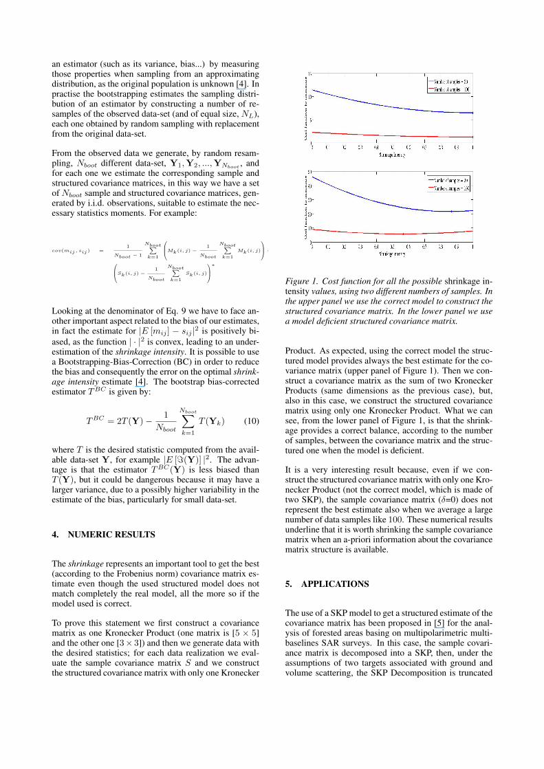
Figure 1. Cost function for all the possible shrinkage in-tensity values, using two different numbers of samples. Inthe upper panel we use the correct model to construct thestructured covariance matrix. In the lower panel we usea model deficient structured covariance matrix.

Product. As expected, using the correct model the struc-tured model provides always the best estimate for the co-variance matrix (upper panel of Figure 1). Then we con-struct a covariance matrix as the sum of two KroneckerProducts (same dimensions as the previous case), but,also in this case, we construct the structured covariancematrix using only one Kronecker Product. What we cansee, from the lower panel of Figure 1, is that the shrink-age provides a correct balance, according to the numberof samples, between the covariance matrix and the struc-tured one when the model is deficient.

It is a very interesting result because, even if we con-struct the structured covariance matrix with only one Kro-necker Product (not the correct model, which is made oftwo SKP), the sample covariance matrix (δ=0) does notrepresent the best estimate also when we average a largenumber of data samples like 100. These numerical resultsunderline that it is worth shrinking the sample covariancematrix when an a-priori information about the covariancematrix structure is available.

5. APPLICATIONS

The use of a SKP model to get a structured estimate of thecovariance matrix has been proposed in [5] for the anal-ysis of forested areas basing on multipolarimetric multi-baselines SAR surveys. In this case, the sample covari-ance matrix is decomposed into a SKP, then, under theassumptions of two targets associated with ground andvolume scattering, the SKP Decomposition is truncated

by retaining only the first two terms.

The multi-images DInSAR framework is slightly differ-ent from the polarimetric one. In this case the two kindsof diversities are time (temporal baselines) and space(normal baselines), and the structure of the covariancematrix is different. For this application we talk about co-herence matrix (Γ) as the covariance matrix is normal-ized by the signal energies in each image. This operationis performed in order to compensate for the backscatteredpower unbalances among all the images.

Consider a data vector y constituted of NI images, underthe same hypotheses previously introduced, the elementsof the coherence matrix can be expressed as:

Γ(n,m) = γSNRΓt(Btn, Btm)Γn(Bnn, Bnm)

n,m = 1 : NI(11)

where Btk and Bnk represent respectively the temporaland normal baselines of k − th image, Γt and Γn takeinto account the losses in coherence due to temporal andnormal baselines of the images used to construct the inter-ferogram and γSNR measures the random noise presentin the radar measurements. In matrix notation we get:

Γ = γSNRΓt ◦ Γn (12)

where ◦ is the Hadamard Product (HP). It is important topoint out this matrix notation as there is a strict relation-ship between the Hadamard and the Kronecker Product:the HP is a sub-matrix of the KP. One difference betweenPolInSAR and DInSAR is that the satellite does not ac-quire data from all the possible geometries (normal base-lines) every time: this is the reason we lose the Kroneckerstructure and we get the Hadamard one.

For this application we introduce another hypothesis, thatis also a constraint: spatial and temporal decorrelationmechanisms must change slowly with the change of thebaselines, in other words they must present a low-pass be-havior. This is a realistic and very common assumption inSAR interferometry: the spatial decorrelation decreaseslinearly with the normal baseline, the temporal one doesnot have a known shape but it is generally assumed tochange slowly in time [1]. In many cases for example anexponential decay model is used for the temporal lossesin coherence. In Figure 2 we present an example of spa-tial and temporal coherence matriciesx with a low-passbehavior, and in Figure 3 the coherence matrix obtainedas the HP of these two matrices (sorted respect to the tem-poral baselines).

Thanks to this assumption, we can interpolate the coher-ence in correspondence of all the possible combinationsamong temporal and spatial baseline, in this way we re-construct the KP as shown in Figure 4.

Then we use the SKP Decomposition and truncate the re-sult at the first KP as we assume only one target. Thanksto this algorithm, other than providing a structured co-variance matrix, we can estimate Γt and Γn, except for

(a) (b)

Figure 2. Right panel: Temporal coherence matrix, theimages are sorted according with the temporal baselines.Left panel: Spatial coherence matrix, the images aresorted according with the normal baselines

Figure 3. Coherence matrix obtained as the HP of thetwo matrices shown in Figure 2, sorted according withthe temporal baselines.

Figure 4. Matrix with KP structure, obtained interpolat-ing the data for all the possible combination of normaland temporal baselines.

(a) (b)

Figure 5. Temporal and spatial coherence matrices esti-mates.

a scaling factor [5], without any physical model for thetemporal decorrelation. In Figure 5 we show the esti-mates for the temporal and spatial coherence matricespresented in Figure 2. This decomposition can be veryuseful as it makes possible a separate analysis for the tar-get location and displacement, reducing the costs and theproblems of a joint analysis.

From the matrix built using the first term of the SKP De-composition, we select the sub-matrix corresponding tothe HP to get the structured coherence matrix, then theshrinkage is used to find the optimal coherence matrixestimate.

An experiment on synthetic data has been performed us-ing a data-set of 20 SAR images, we considered a modelfor the spatial decorrelation decreasing with the normalbaseline and a seasonal model for the temporal decorrela-tion (usually we find high coherence during summer andlow coherence during winter), both with a low-pass be-havior (Figure 2 and Figure 3). Then we generated data-set with different numbers of data samples and found theoptimal shrinkage intensity, knowing the real coherencematrix. From each data simulation we estimated the opti-mal shrinkage intensity, using Eq 9 and the bootstrappingto infer the necessary statistics moments, then we evalu-ated the mean value of the δ estimates. The results areplotted in Figure 6.

Figure 6. Shrinkage Intensity for different numbers ofdata samples.

Also in this case we can notice how the shrinkage pro-vides a better estimate for the coherence matrix, espe-cially when we have a small number of pixels for the esti-mate. It also worth noticing that the estimates for δ, fromthe data, are lightly underestimated respect to the effec-tive optimal shrinkage intensity due to the positive biasof the estimate of the denominator in Eq 9, as discussedin III.A. In particular the bias is more evident for smallnumber of samples, as the higher is the number of sam-ples the more reliable is the bias estimator. Notwithstand-ing the shrinkage intensity estimates are underestimated,the shrinkage estimator provides the same a better esti-mate for the coherence matrix than the sample estimatoras shown in Figure 7.

Figure 7. Frobenius norm of the estimation error (Eq. 8)using the optimal shrinkage intensity, using its estimateand using only the sample estimator.

6. CONCLUSION

In this work we proved how we should not trust blindlyin the observed data: in fact the sample covariance isthe best estimator when no other information is avail-able. The aim of the shrinkage is to find the right bal-ance between the sample and the a-priori information,by computing a convex linear combination between thesample and the structured covariance matrices. In par-ticular we focused on matrices based on SKP model, theadvantages are the velocity of the SKP Decompositionand the possibility to get a structured model without anyphysical assumption, using only statistical hypotheses. Inadd we proved that the SKP-shrinkage is suitable to im-prove the estimate for coherence matrices constructed asthe Hadamard Product of two matrices with a low-passbehavior. A semi-analytic formulation to estimate the op-timal shrinkage intensity from the observed data (withoutknowing the real covariance matrix: as in all the practicalcases) has been provided, keeping in mind that tends tobe underestimated due to bias problem.

REFERENCES

[1] A. Ferretti, A. Monti Guarnieri, C. Prati andF. Rocca, InSAR Principles: Guidelines for SAR In-

terferometry Processing and Interpretation, 1rd ed.ESA Pubblications, 2007.

[2] O. Ledoit, M. Wolf, Improved estimation of the co-variance matrix of stock returns with an applicationto portfolio selection, Journal of Empirical Finance,September 2002.

[3] O. Ledoit, M. Wolf, Honey I Shrunk the sample co-variance matrix, Journal of Portfolio Managment,Vol 30, Number 4, 2004.

[4] J. Shao and D. Tu, The Jackknife and Bootstrap,2rd ed. Springer, 1996.

[5] S. Tebaldini, Algebraic Synthesis of Forest ScenariosFrom Multibaseline PolInSAR Data, IEEE Transac-tions on Geoscience and Remote Sensing, to be pub-lished

[6] C. Van Loan and N. Pitsianis ”Approximation withKronecker Products” in Linear Algebra for LargeScale and Real Time Applications, M.S.Moonen,G.H. Golub, and B.L. R.De Moor, Eds. Norwell,MA:Kluwer, 1993, pp. 293-314.