1 23 Transport in Porous Media ISSN 0169-3913 Volume 87 Number 3 Transp Porous Med (2011) 87:717-737 DOI 10.1007/ s11242-010-9711-8 Homogenization of Hydraulic Conductivity for Hierarchical Sedimentary Deposits at Multiple Scales

Welcome message from author
This document is posted to help you gain knowledge. Please leave a comment to let me know what you think about it! Share it to your friends and learn new things together.
Transcript
1 23
Transport in Porous Media ISSN 0169-3913Volume 87Number 3 Transp Porous Med (2011)87:717-737DOI 10.1007/s11242-010-9711-8
Homogenization of HydraulicConductivity for Hierarchical SedimentaryDeposits at Multiple Scales

1 23
Your article is protected by copyright and
all rights are held exclusively by Springer
Science+Business Media B.V.. This e-offprint
is for personal use only and shall not be self-
archived in electronic repositories. If you
wish to self-archive your work, please use the
accepted author’s version for posting to your
own website or your institution’s repository.
You may further deposit the accepted author’s
version on a funder’s repository at a funder’s
request, provided it is not made publicly
available until 12 months after publication.

Transp Porous Med (2011) 87:717–737DOI 10.1007/s11242-010-9711-8
Homogenization of Hydraulic Conductivityfor Hierarchical Sedimentary Deposits at MultipleScales
Ye Zhang · Baozhong Liu · Carl W. Gable
Received: 18 May 2010 / Accepted: 30 December 2010 / Published online: 14 January 2011© Springer Science+Business Media B.V. 2011
Abstract Based on a three-dimensional heterogeneous aquifer model exhibitingnon-stationary, statistically anisotropic correlation, three hydrostratigraphic models (HSMs)are created within a sedimentary hierarchy. A geostatistical analysis of natural log conduc-tivity (lnK ) is conducted for the units of the HSMs. Hydraulic conductivity is then upscaledusing numerical and analytical methods. Increasing lnK variances are evaluated. Resultssuggest that for the aquifer model tested: (1) the numerical method is capable of upscalingirregular domains with reasonable accuracy for a lnK variance up to 7.0. (2) Accuracy ofthe upscaled equivalent conductivities (K∗) and associated performance of the HSMs aresensitive to homogenization level, heterogeneity variance, and boundary condition. Varianceis found to be the most significant factor impacting the accuracy of the HSMs. (3) Diagonaltensor appears a good approximation for the full-tensor K∗. (4) For the HSM units, when thevariance is low (less than 1.0), all analytical methods are nearly equally accurate; however,when variance becomes higher, analytical methods generally are less accurate.
Keywords Hydraulic conductivity · Heterogeneity · Upscaling ·Equivalent conductivity · Sedimentary hierarchy
1 Introduction
Environmental and petroleum studies have documented that spatial variation in hydraulicconductivity (K ), or conductivity heterogeneity, is the rule rather than exception in natural
Y. Zhang (B)University of Wyoming, 1000 University Ave., Laramie, WY 82071, USAe-mail: [email protected]
B. LiuUniversity of Wyoming, Laramie, WY 82071, USA
C. W. GableLos Alamos National Lab, Los Alamos, NM 87545, USA
123
Author's personal copy

718 Y. Zhang et al.
sedimentary rocks. In aquifers, conductivity heterogeneity is found to control the locationand pathway of groundwater flow (thus the movement of dissolved solutes in groundwater).In petroleum reservoirs, heterogeneity of permeability is of interest. Since the advent ofmodern computers, subsurface fluid processes are evaluated quantitatively using simulationmodels. Such models are commonly constructed with site geological and/or geophysical data,populated with appropriate parameters (e.g., conductivity and storage coefficient in aquifers,permeability and rock/fluid compressibility in reservoirs), calibrated based on observed fluidpotential and flow rate data, and then used for predictions for aquifer or reservoir manage-ment. However, detailed subsurface heterogeneity is rarely incorporated into the models,due to the prohibitive cost of conducting subsurface sampling over large spatial scales andcomputation limitation.
Because of the known impact of heterogeneity on subsurface fluid flow, some level ofK (or permeability) variation is incorporated in models, though most do not account forheterogeneity down to the smallest resolvable continuum scale (e.g., core measurements).For example, heterogeneity is sometimes populated throughout a model grid via geostatis-tical means, i.e., each grid cell is given a grid conductivity which accounts for bulk flowbehaviors arising out of the unresolved sub-grid heterogeneities. On the other hand, whenmultiple aquifer or reservoir layers exist, heterogeneity can be represented by a series ofinternally homogeneous units to represent important flow pathways or barriers. In petroleumstudies, using outcrop, well log, or high-resolution seismic data, facies or facies assemblagemodeling can identify zones of relative homogeneity at even finer scales. This second typeof heterogeneity representation, relevant in field- and larger scale modeling, is referred to asa hydrostratigraphic model (HSM).
In sedimentary rocks, depositional structures can exist at multiple scales which determinethe spatial variation of K . Division of HSM units is thus non-unique, their creation constrainedby model scale, processes of interest (e.g., fluid flow versus species transport), computingpower, or type and availability of site characterization data. Regardless of the simulationgoal, equivalent conductivity (or equivalent permeability) is required for the model units,to represent the effect of unresolved, sub-unit-scale heterogeneity on bulk flow prediction.This upscaling should be distinguished from the body of work conducted in coarse-grainingresearch (Sanchez-Vila et al. 1995, 1996; Wen and Gómez-Hernández 1996; Renard andde Marsily 1997; Durlofsky 2005; Sanchez-Vila et al. 2006). Typically, in such studies, ahigh-resolution geological model is upscaled to a coarsened flow simulation grid in order toachieve computation efficiency in flow modeling.
In this study, single-phase water flow is of interest, thus conductivity is the parameterevaluated. Based on a three-dimensional (3D) heterogeneous model exhibiting non-station-ary, statistically anisotropic correlation structure, a set of nested HSMs is created within asedimentary hierarchy. For units of these models, equivalent conductivity (K∗) are estimatedusing numerical and analytical upscaling methods. A sensitivity analysis is conducted byscaling the heterogeneous model to multiple natural log conductivity (lnK ) variances. Ateach variance, upscaling is repeated. Both variance and homogenization level are thus evalu-ated to understand their impact on K∗ and accuracy of the HSMs in single-phase predictions.Note that for two aquifer models, one with geometric connectivity and one without, an earlierstudy has compared their scaling characteristics using similar techniques (Zhang et al. 2010).The unique aspect of this study is the evaluation of sub-aquifer heterogeneities at multiplescales, which the earlier study did not address.
In the reminder of this article, creation of the models is described, followed by descriptionsof a geostatistical analysis and the numerical and analytical upscaling methods. Section 3presents the upscaled conductivities: those computed by the numerical method are verified
123
Author's personal copy

Homogenization of Hydraulic Conductivity 719
Fig. 1 a Heterogeneous model with local K in natural log scale (here, lnK variance=16); b DepositionalModel with 3 units: upper channel belt, upper sheetflow, and lower sheetflow. Unit ID is shown. c FaciesModel with 8 units. Unit ID is shown. d Visualization of units 1, 2, and 3 of the Facies Model
by conducting flow simulations in all models. Accuracy of the HSMs in predicting flow rateand fluid potential of the heterogeneous model is discussed. Prediction sensitivity to lnKvariance is highlighted. Linkage among conductivities homogenized at different scales isexplored. Conductivity upscaled by analytical methods is presented next, their limitationsdiscussed. Finally, results are summarized and directions for future research are presented.
2 Methods
2.1 Model Construction
Three HSMs are created from a heterogeneous model within a single grid structure: theheterogeneous model has spatially variable conductivities (Fig. 1a), the HSMs have homog-enized units with upscaled K∗ (Fig. 1b, c, d). Details on creating the heterogeneous model aredescribed elsewhere (Zhang et al. 2010). Below sections describe the creation of the HSMs.
The HSMs are created within a 3-tier sedimentary hierarchy: (1) a Full Aquifer Model(1-unit model); (2) a Depositional Model (3-unit model) (Fig. 1b); and (3) a Facies Model(8-unit model) (Fig. 1c). Identification number for each unit is labeled on the models. Inthe facies and depositional models, all units are irregular, created with the following steps.First, we start with the most refined model—the Facies Model. Delineation of units in this
123
Author's personal copy

720 Y. Zhang et al.
Fig. 2 Directional experimental variograms of lnK (circles) for the upper channel belt (unit 1 of the Depo-sitional Model). Three exponential models are fitted (curves). Global aquifer lnK variance is 0.1. Since theupper channel belt is only a part of the aquifer, its variance is lower (0.078)
model is based on visual inspection of stratigraphic contacts and/or changes in dominantheterogeneity style. Four steps are used: (1) the heterogeneous model is dissected into 26two-dimensional slices at x = 10, 100, 200, . . . , 2400, 2500 m; (2) correlatable stratigraphiccontacts are traced on each image, their coordinates (i.e., (y, z) values of points along thecontacts) recorded at each x . For the 8 units of the Facies Model, 12 curvilinear contacts aredefined on each image; (3) by pooling together all images, 12 correlated surfaces are createdusing Ordinary Kriging interpolation (for each surface, a global omnidirectional experimen-tal variogram of z is computed and fitted with a Gaussian model whose parameters are usedin kriging); (4) using the gridding toolbox lagrit (www.lagrit.lanl.gov), these surfaces areimported into the 3D grid and used to divide the model into different facies units.
Since the upper portion of the deposits appears more channelized than the lower portion,all cells of the Facies Model are recolored to assemble and regroup the units into 3 Deposi-tional Model units: Upper Channel Belt, Upper Sheetflow Belt, and Lower Sheetflow Belt(Fig. 1b). Units 1, 2, 3 of the Facies Model become channel facies of unit 1 of the Depositional
123
Author's personal copy

Homogenization of Hydraulic Conductivity 721
Model, while unit 4 becomes the background floodplain facies of unit 1 of the same model.Unit 5 of the Facies Model is now sheetflow facies of unit 2 of the Depositional Model, whileunit 6 is the background floodplain facies of the same unit. The Full Aquifer Model (notshown) incorporates all units of the Depositional Model. It has the highest level of hierarchyfor which a natural analog could be a geological formation. Since only one unit exists in thismodel, it also has the greatest volume for conductivity homogenization.
In the above analysis, a set of sedimentary criteria is used to correlate and map the sub-aquifer hierarchy. The division adopted, however, is non-unique. For example, by creatingmore stratigraphic contacts within facies, a HSM can be created at sub-facies scale, andaccordingly, units for homogenization will be more numerous. However, the current divisionreflects the current heterogeneity complexity in the aquifer. Since the mapping approach isflexible, as is the numerical upscaling method (presented next), the study methodology isapplicable to any dataset and any interpretation.
In this study, the heterogeneous model is first scaled to 4 global lnK variances: 0.1, 1.0,7.0, 16.0, spanning the full range of variability representing weakly to strongly heteroge-neous deposits (Gelhar 1993). During this scaling, the same mean lnK value (3.67 m/y) ismaintained. Thus, four populations of conductivity are created and subsequently upscaled.In a practical sense, this scaling reflects the certainty of heterogeneity pattern (e.g., fromseismic interpretations), but uncertainty of the level of variability of heterogeneity (Millikenet al. 2007).
2.2 Spatial Correlations
Geostatistical characteristics of each unit of the HSMs are evaluated by computing threedirectional experimental lnK variograms: two horizontal (one along x , one along y), onevertical. Given the cellwise coloring of unit IDs, variogram computation for the units isstraightforward, i.e., variogram pairs are selected not only based on separation vectors butalso based on unit IDs (more details can be found in Zhang 2008). Variograms of the FullAquifer model was presented in Zhang et al. (2010). Figure 2 presents the variograms of theUpper Channel Belt of the Depositional Model. In this figure, lnK variance is 0.1. Scalingof lnK variance will proportionally scale the variogram sill without affecting the correla-tion ranges. Similar variograms are computed for all the HSM units (not shown). With theexception of two lateral-direction periodic structures, all variograms exhibit exponential-likebehavior, thus exponential models are fitted to the experimental variograms and directionalintegral scales are estimated (Table 1).
From the variograms, we observe: (1) both the integral scales and associated statisticalanisotropy ratios (e.g., λx/λz, λy/λz) fall within the range found for natural fluvial deposits(Deutsch 2002), suggesting that the model grid cell size and aspect ratio are reasonable;(2) both horizontal integral scales are significantly larger than the vertical integral scale, lnKof all units is thus statistically anisotropic; (3) variogram spatial correlation is not axisym-metric, i.e., the two horizontal integral scales are not equal. For all units and at all scales,λy > λx
1; (4) correlation characteristics of the HSM units are similar at different scales.With few exceptions, lnK variograms exhibit exponential rises towards the sills, which canbe explained by the observed stratification (Fig. 1a). Detailed field mapping of conductivity
1 A plausible explanation for the larger length of continuity along y is that sediment transport in the physicalexperiment from which the heterogeneous model of this study is derived occurred along the y-axis (Zhang et al.2010). It is also possible that since the heterogeneous model is interpolated among 16 images perpendicularto y, y-directional continuity was enhanced by this procedure (Zhang et al. 2010).
123
Author's personal copy

722 Y. Zhang et al.
Tabl
e1
Stat
istic
alpa
ram
eter
sof
the
3hy
dros
trat
igra
phic
mod
els
Hyd
rost
ratig
raph
icm
odel
sU
nitI
DN
umbe
rof
grid
cells
Glo
ball
nKva
rian
cea
Fitte
din
tegr
alsc
ales
(m)
0.1
1.0
7.0
16.0
λx
λy
λz
E[l
nK]
Var
[lnK
]E
[lnK
]V
ar[l
nK]
E[l
nK]
Var
[lnK
]E
[lnK
]V
ar[l
nK]
Full
Aqu
ifer
Mod
el1
4182
413.
668
0.1
3.66
81.
03.
668
7.0
3.66
816
.015
5.0
690.
05.
0
Dep
ositi
onal
Mod
el1
2047
283.
496
0.07
83.
124
0.78
42.
229
5.48
71.
492
12.5
4315
5.0
610.
03.
8
299
669
3.86
10.
066
4.28
00.
662
5.28
84.
632
6.11
710
.586
140.
090
0.0
12.0
311
3844
3.80
70.
063
4.11
00.
629
4.83
74.
404
5.43
610
.066
200.
090
0.0
12.0
Faci
esM
odel
116
696
3.72
40.
046
3.84
60.
458
4 .14
03.
208
4.38
27.
333
155.
061
0.0
3.5
222
559
3.75
70.
048
3.94
90.
482
4.41
23.
373
4.79
37.
709
135.
032
0.0
3.0
328
221
3.77
10.
037
3.99
50.
373
4.53
42.
612
4.97
75.
971
135.
070
0.0
3.4
413
7252
3.36
80.
046
2.72
10.
464
1.16
33.
248
0.11
97.
423
155.
025
0.0
3.0
517
422
4.16
80.
027
5.25
00.
266
7.85
31.
859
9.99
54.
248
155.
027
5.0
7.5
682
247
3.79
60.
050
4.07
50.
504
4.74
43.
529
5.29
58.
067
155.
072
0.0
15.0
713
070
4.07
90.
044
4.96
70.
437
7.10
63.
056
8.86
56.
984
230.
030
0.0
3.0
810
0774
3.77
20.
055
3.99
80.
546
4.54
33.
825
4.99
18.
743
330.
035
0.0
16.0
a Hyd
raul
icco
nduc
tivity
(K)
isin
m/y
.Glo
ball
nKva
rian
ceis
the
vari
ance
ofln
Kfo
rth
efu
llaq
uife
rm
odel
.E[l
nK]
isth
em
ean
lnK
.Var
[lnK
]is
the
vari
ance
ofln
K
123
Author's personal copy

Homogenization of Hydraulic Conductivity 723
in channelized systems has linked such behaviors to multiple scales of juxtaposing units ofcontrasting conductivities (Ritzi and Allen-King 1986).
Correlation parameters for each unit, along with the mean and variance of lnK , will beused by select analytical methods to predict an equivalent or effective conductivity, to becompared to the results of numerical upscaling. Though not presented, histograms of lnK ofmost units are unimodal, with probability densities approaching normal distributions. Thus,though the conductivity field as a whole exhibits non-multiGaussian characteristics (e.g., dis-tinct existence of channel connectivity, heterogeneity non-stationarity ranging from channelto sheetflow dominated), its univariate and bivariate statistics closely satisfy most analyticaltheory requirements (Sect. 2.4). This is because bivariate correlation functions cannot distin-guish either the existence, or lack of existence, of important spatial connectivity as observedin natural heterogeneity (Knudby and Carrera 2005, 2006).
2.3 Numerical Upscaling
To calculate an equivalent conductivity (K∗), numerical upscaling is conducted by simulat-ing flow in the heterogeneous model, based on and in extension to earlier studies (Zhanget al. 2006, 2010). To find K∗ for a HSM unit, a series of single-phase, steady-state, andincompressible flow simulations are conducted in the heterogeneous model by varying theboundary condition along the model periphery. An equivalent K∗ is obtained by incorporat-ing results from all simulations. For each unit, a set of equations is assembled, consisting ofspatially averaged directional hydraulic gradients, Darcy fluxes, and equivalent conductivitytensor components:⎡⎢⎢⎢⎢⎢⎢⎢⎢⎢⎢⎢⎢⎢⎢⎢⎢⎢⎢⎢⎢⎣
〈∂h/∂x〉1 〈∂h/∂y〉1 〈∂h/∂z〉1 0 0 0 0 0 00 0 0 〈∂h/∂x〉1 〈∂h/∂y〉1 〈∂h/∂z〉1 0 0 00 0 0 0 0 0 〈∂h/∂x〉1 〈∂h/∂y〉1 〈∂h/∂z〉1
〈∂h/∂x〉2 〈∂h/∂y〉2 〈∂h/∂z〉2 0 0 0 0 0 00 0 0 〈∂h/∂x〉2 〈∂h/∂y〉2 〈∂h/∂z〉2 0 0 00 0 0 0 0 0 〈∂h/∂x〉2 〈∂h/∂y〉2 〈∂h/∂z〉2. . . . . . . . . . . . . . . . . . . . . . . . . . .
〈∂h/∂x〉m 〈∂h/∂y〉m 〈∂h/∂z〉m 0 0 0 0 0 00 0 0 〈∂h/∂x〉m 〈∂h/∂y〉m 〈∂h/∂z〉m 0 0 00 0 0 0 0 0 〈∂h/∂x〉m 〈∂h/∂y〉m 〈∂h/∂z〉m0 1 0 −1 0 0 0 0 00 0 1 0 0 0 −1 0 00 1 0 0 0 1 0 −1 0
⎤⎥⎥⎥⎥⎥⎥⎥⎥⎥⎥⎥⎥⎥⎥⎥⎥⎥⎥⎥⎥⎦
·
⎧⎪⎪⎪⎪⎪⎪⎪⎪⎪⎪⎪⎪⎨⎪⎪⎪⎪⎪⎪⎪⎪⎪⎪⎪⎪⎩
Kxx
Kxy
Kxz
Kyx
Kyy
Kyz
Kzx
Kzy
Kzz
⎫⎪⎪⎪⎪⎪⎪⎪⎪⎪⎪⎪⎪⎬⎪⎪⎪⎪⎪⎪⎪⎪⎪⎪⎪⎪⎭
= −
⎧⎪⎪⎪⎪⎪⎪⎪⎪⎪⎪⎪⎪⎪⎪⎪⎪⎪⎪⎪⎪⎨⎪⎪⎪⎪⎪⎪⎪⎪⎪⎪⎪⎪⎪⎪⎪⎪⎪⎪⎪⎪⎩
〈qx 〉1⟨qy
⟩1〈qz〉1
〈qx 〉2⟨qy
⟩2〈qz〉2
. . .
〈qx 〉m⟨qy
⟩m〈qz〉m
000
⎫⎪⎪⎪⎪⎪⎪⎪⎪⎪⎪⎪⎪⎪⎪⎪⎪⎪⎪⎪⎪⎬⎪⎪⎪⎪⎪⎪⎪⎪⎪⎪⎪⎪⎪⎪⎪⎪⎪⎪⎪⎪⎭
(1)
where 〈 〉 represents spatial averaging among grid cells of a HSM unit; qx , qy, qz are compo-nents of the Darcy flux; h is hydraulic head; subscripts 1, 2, . . . , m denote flow experiments
123
Author's personal copy

724 Y. Zhang et al.
driven by different global boundary conditions; Kxx , . . . , Kzz are components of the equiv-alent K∗. To obtain a unique solution, the total number of flow experiments m must be ≥3.For the above non-square system (e.g., Ax = b), Eq. 1 is solved via least square solution,i.e., x is determined by minimizing the 2-norm of the residual vector r = Ax − b, where
2-norm is defined as ||r||2 =√∑3m+3
i=1 (r2i ).
Within the context of the upscaling literature, the above method is global in nature: K∗ ofa particular upscaling domain (e.g., a HSM unit) is calculated using averages of head gra-dients and fluxes which are computed from global flow simulations that extend beyond theparticular domain. Further, symmetry in K∗ is ensured by adding 3 constraint equations onthe off-diagonal terms. This procedure is a more natural approach compared to those of ourearlier studies (symmetry is imposed after solving the off-diagonal components), althoughscaling of the constraint equations by a number consistent with the magnitude of the gra-dient components may be necessary to reduce numerical truncation error. As discussed byWen et al. (2003), positive-definiteness of K∗ cannot be assured by this procedure. Thus, foreach HSM unit, after K∗ is computed by Eq. 1, test is conducted to ensure that the result isphysically correct (e.g., eigen values of K∗ are positive).
The size of Eq. 1 is controlled by m which is ideally a large number simulating manyboundary conditions. The system is thus subjected to many types of flow stimulation so thata representative conductivity may be found that is less dependent on the boundary condition.In earlier studies, we found that when the upscaling domain was large compared to lnKintegral scales, K∗ became insensitive to boundary condition and the number of flow experi-ments, thus smaller m may be used (Zhang et al. 2006). However, the set of experiments mustbe carefully chosen so that each will result in a flow field that is distinct from the others. Thismeans that similar boundary condition will not be used, e.g., imposing a higher gradient todrive flow compared to a previous experiment using a lower gradient. Moreover, although theglobal method is computationally more expensive than the various local methods, they canbe more accurate since flow channeling due to conductivity connection outside the upscalingdomain can be accounted for in computing K∗. This is affirmed by observations that accuracyof a local method improves when the size of the upscaling region surrounding each grid cellincreases (Wen et al. 2003).
Numerical upscaling results are compared to the results of several analytical methodsdeveloped under mean uniform flow conditions, thus linear flood patterns are used in the flowexperiments (analytical expressions developed for radial flows with source or sink terms arenot investigated). For each HSM unit, Eq. 1 is assembled based on 3 sets of global boundaryconditions (m = 3): (1) x-flow (specified heads along the left and right faces of the model;no-flow on all other faces); (2) y-flow (specified heads along the front and back faces; no-flowon all other faces); (3) z-flow (specified heads along the top and bottom faces; no-flow on allother faces). More details on these experiments and the effort involved in code verificationcan be found in Zhang et al. (2010).
2.4 Analytical Upscaling
Several analytical methods exist that are applicable to upscaling statistically anisotropicmedia. For example, power law was proposed as an approach for equivalent conductivityestimation (Journel et al. 1986):
K j j =[
1
N
N∑i=1
Kp ji
]1/p j
( j = 1, . . . , 3) (2)
123
Author's personal copy

Homogenization of Hydraulic Conductivity 725
where N is number of local conductivities (Ki ), K j j is principal components of the equivalentconductivity, p j is the corresponding directional power-averaging exponent. −1 ≤ p j ≤ 1:when p j = −1, K j j is the harmonic mean (KH); when p j = 1, K j j is the arithmetic mean(KA); when p j → 0 in the limit, K j j becomes the geometric mean (KG). For statisticallyanisotropic media, p j is estimated by Ababou (1991) as:
p j = 1 − 2
3
λHarmo
λ j( j = 1, . . . , 3) (3)
where λ j is directional lnK integral scales, λHarmo is their harmonic mean estimated by:
λHarmo =⎡⎣1
3
3∑j=1
λ−1j
⎤⎦
−1
(4)
Equations 2–4 can be used to predict equivalent conductivity principal components, giventhe local conductivities and directional lnK integral scales.
For multiGaussian media, Desbarats (1992) also proposed a power law method, althoughthe power-averaging exponents were obtained from numerical upscaling:
ln(K j j ) = μ f + p j
2σ 2
f ( j = 1, . . . , 3) (5)
where μ f and σ 2f are expected value and variance of local point-scale lnK , respectively. In
this study, Eq. 5 is tested by applying the directional exponent (p j ) obtained from Eq. 2—p j
is calculated by equating Eq. 2 with the principal components of the upscaled K∗.Based on the Green’s function, another expression using p j was derived for a multiGaus-
sian medium of a large extent (i.e., domain length greater than lnK integral scales) (Noetingerand Haas 1996):
K j j = KG exp(p jσ2f /2) ( j = 1, . . . , 3) (6)
Equation 6 was numerically verified to be accurate for lnK variances up to 1.0.In a stationary medium with low variance, an effective conductivity expression was devel-
oped based on KG, σ 2f , and lnK integral scales (Gelhar and Axness 1983):
K j j = KG
[1 + σ 2
f
(1
2− g j j
)]( j = 1, . . . , 3) (7)
where g j j is a complex multidimensional integral. For an axisymmetrical medium (e.g.,λ1 = λ2 > λ3) with exponential correlation functions, g j j becomes:
g11 = g22 = 1
2
1
ρ2 − 1
[ρ2
√ρ2 − 1
tan−1(√
ρ2 − 1) − 1
]
g33 = ρ2
ρ2 − 1
[1 − 1√
ρ2 − 1tan−1(
√ρ2 − 1)
](8)
where ρ = λ1/λ3 > 1. This result was tested and expanded by prior authors, e.g., see reviewin Zhang (2002). For statistically anisotropic media, it was found accurate for low variances(e.g., less than 1.0). In this study, λx and λy are averaged to obtain a λ1, representing a hori-zontal integral scale from modeling an omnidirectional horizontal variogram. Further, basedon the Landau–Lifshitz conjecture, a high variance version of Eq. 7 is postulated, which treatsthe two terms within the brackets of Eq. 7 as part of a series expansion of an exponential
123
Author's personal copy

726 Y. Zhang et al.
function: K j j = KG exp[σ 2
f
( 12 − g j j
)](Gelhar and Axness 1983). This formulation has
not been tested extensively.Following the same arguments of Gelhar and Axness (1983), a simplified formula is
proposed and generalized to higher variances (Ababou 1996):
K j j = KG exp
[σ 2
f
(1
2− 1
3
λHarmo
λ j
)]( j = 1, . . . , 3) (9)
Among the formulations, those based on stochastic theories aim to predict an ensembleeffective conductivity of a random field, thus rigorous comparison between equivalent andeffective conductivity will require a stochastic Monte Carlo analysis. In this study, rather thanvalidating theories, we are interested in whether theories can be used to predict propertiesconsistent with upscaling results from a single realization, following Zhang et al. (2006),Desbarats and Srivastava (1991). Within the stochastic framework, an argument can alsobe made that in evaluating single realizations, if the domain size is large compared to lnKintegral scale (this has been assured by the geostatistical analysis; Table 1), an ergodic limitcan be reached whereby deterministic spatial average coincides with ensemble average.
3 Results and Discussions
3.1 Upscaled Conductivities
For each unit of the HSMs, K∗ is computed with Eq. 1, at 4 global lnK variances (σ 2f =
0.1, 1.0, 7.0, 16.0). Since conductivity must be positive definite, Cholesky factorization isused to test K∗. With four exceptions, the majority of K∗ (44 tensors) passes the test (Table 2lists the principal components). The four that fail the test belong to unit 3 of the Depositionalmodel and units 5, 7, and 8 of the Facies model, respectively, when σ 2
f = 16.0. A commoncharacteristics among them is an extremely small and negative K33 (principal component ofK∗ along z), compared to a positive and much larger K11 (principal component along x) andK22 (along y). Since 16 is considered a high variance, a likely cause for non-positive-defi-niteness is extreme flow channeling in the horizontal direction. In the aquifer model, a priorpercolation analysis has identified a high-K connected structure spanning the lower domainalong x—in the same region of the model containing these units (Zhang et al. 2010). At thesame high variance, however, eight other units pass the test—these are located outside thespanning cluster. It is likely that the upscaled K∗ is inaccurate when high variance coincideswith geometric connectivity. These four tensors are excluded in the following analysis.
For all units, at all variances, most K∗ are diagonally dominant reflecting horizontal stratifi-cation (Fig. 1a). Since diagonal dominance of upscaled K∗ is an indication that lnK statisticalaxes are aligned with the global coordinate axes (Gelhar 1993), geostatistical analysis of thisstudy is thus appropriate (it is carried out independently of the upscaling calculations). Sincemost analytical methods are based on the same assumption, diagonal dominance simplifiesthe comparison between numerical and analytical results.
K∗ computed for the Full Aquifer Model are compared to the diagonal tensors computedfor the same model using the Simple Laplacian (SL) method (Renard and de Marsily 1997).SL is a local method that is applicable to upscaling rectangular or box-shaped media. It isused to compute Kxx , Kyy , and Kzz of the Full Aquifer Model. Note that when applyingEq. 1 to the full aquifer, the global method is reduced to a local method. Due to diagonaldominance, Kxx , Kyy , and Kzz are comparable with K11, K22, and K33. For the Full Aquifer
123
Author's personal copy

Homogenization of Hydraulic Conductivity 727
Tabl
e2
Equ
ival
entc
ondu
ctiv
itypr
inci
palc
ompo
nent
sco
mpu
ted
with
Eq.
1fo
ral
lthe
HSM
units
Stra
tigra
phic
Mod
els
Uni
tID
Dep
ositi
onty
peG
loba
llnK
vari
ance
0.1
1.0
7.0
16.0
Ka 11
K22
K33
K11
K22
K33
K11
K22
K33
K11
K22
K33
Aqu
ifer
Eq.
1A
fluvi
alsy
stem
40.9
6840
.101
38.1
5360
.736
50.3
2033
.434
514.
172
185.
345
34.0
5252
01.0
0070
6.50
088
.800
Mod
elSL
b40
.981
40.1
4738
.434
60.7
4750
.432
34.2
9551
2.72
418
5.89
636
.176
5183
.03
713.
983
96.4
40
Dep
ositi
onal
Mod
el1
Cha
nnel
ized
34.1
3033
.318
42.7
8132
.556
26.0
4746
.955
93.4
0825
.750
65.3
4138
8.85
427
.024
179.
395
2Sh
eetfl
ow48
.970
47.1
5535
.105
96.5
4376
.127
22.7
6611
32.1
0034
5.00
05.
100
1390
3.00
014
13.0
04.
000
3Sh
eetfl
ow46
.266
46.0
7232
.477
80.1
5570
.930
18.2
8073
2.57
432
6.33
72.
579
6249
.800
1142
.600
−0.5
00
Faci
esM
odel
1C
hann
el42
.100
29.8
2336
.670
55.6
6118
.811
24.5
6720
2.01
115
.190
7.52
889
8.47
810
.120
18.0
68
2C
hann
el43
.657
33.9
1043
.457
63.8
7526
.218
47.8
8332
0.48
422
.310
67.9
3413
49.5
0023
.500
283.
800
3C
hann
el44
.035
34.8
4446
.651
62.6
7428
.861
61.9
2124
5.36
028
.183
97.3
4511
59.4
0037
.400
174.
400
4Fl
oodp
lain
29.5
9133
.336
42.6
2318
.656
26.3
3346
.513
12.9
8027
.221
65.8
677.
858
34.9
4818
6.59
2
5Sh
eetfl
ow65
.344
51.7
4233
.610
212.
079
96.2
6419
.762
4744
.400
457.
400
2.80
071
313.
000
1714
.000
−1.0
00
6B
ackg
roun
dc45
.547
46.1
8435
.422
72.9
9171
.816
23.4
0343
4.32
932
0.06
85.
545
2977
.700
1337
.700
4.20
0
7Sh
eetfl
ow59
.965
47.9
6132
.323
171.
447
80.8
7717
.988
3387
.100
460.
900
2.40
034
754.
000
1858
.000
−1.0
00
8B
ackg
roun
dc44
.485
45.8
4732
.497
68.3
3469
.900
18.3
1840
1.01
431
5.42
72.
595
2691
.200
1090
.200
−0.7
00
For
the
Full
Aqu
ifer
Mod
el,t
hepr
inci
palc
ompo
nent
sar
eal
soco
mpu
ted
with
the
Sim
ple
Lap
laci
anM
etho
d.Fo
urof
the
cond
uctiv
ityte
nsor
s,te
sted
tobe
non-
posi
tive-
defi
nite
,ar
eem
phaz
ised
inbo
lda
All
cond
uctiv
itypr
inci
palc
ompo
nent
sar
ein
units
ofm
/yr;
K11
,K
22,a
ndK
33ar
eal
igne
dap
prox
imat
ely
with
the
glob
alx,
y,an
dz
axes
,res
pect
ivel
yb
Sim
ple
Lap
laci
anM
etho
dof
Wen
and
Góm
ez-H
erná
ndez
(199
6)w
hich
com
pute
sa
diag
onal
tens
orfo
rre
ctan
gula
ror
box
shap
edm
edia
cB
ackg
roun
dfa
cies
with
low
erco
nduc
tivity
can
bedi
stin
guis
hed
from
the
high
-Ksh
eetfl
owde
posi
t
123
Author's personal copy

728 Y. Zhang et al.
model, at all variance levels, principal components of K∗ are very close to those computedby the SL method. This serves to verify Eq. 1 for this model.
Comparing the principal components of K∗ of the Full Aquifer Model with those of theDepositional and Facies models, their magnitudes are consistent across scales. Based onthe volumes of the units (i.e., number of grid cells within), weighted arithmetic averages ofappropriate sub-hierarchy conductivity components are calculated (Table 3). These weightedaverages are compared to the corresponding upscaled conductivities of the encompassingunit(s) of higher hierarchy. A set of percent relative errors (RE) is calculated. For example,at the same variance, K11 of the Full Aquifer Model is compared to a weighted average ofK11 of the 3 units of the Depositional Model and a weighted average of K11 of the 8 unitsof the Facies Model, respectively; K11 of unit 1 of the Depositional Model is compared to aweighted average of K11 of units 1, 2, 3, 4 of the Facies Model, etc.
Results suggest that for the given variance range (0.1–7.0), RE is extremely small (oftenless than 0.1%), thus equivalent conductivity principal components of the HSM units at dif-ferent scales are related by volume-weighted arithmetic means. To our knowledge, this isthe first time such a relationship is revealed among conductivities of irregular deposits. It isof interest to note that though harmonic averaging is a popular estimator to relate verticalconductivity at different scales, it is found inaccurate here, particularly when the systemvariance is high (both weighted harmonic mean and harmonic mean have been tested forwhich RE reaches 86% when σ 2
f = 7.0). However, whether this observation is generalizableto other heterogeneities requires additional studies. Since K∗ of the Full Aquifer model isverified by the SL method, this multiscale comparison serves to partially verify K∗ computedfor the facies and depositional models.
Finally, as part of the upscaling procedure, flow simulations are conducted in the heter-ogeneous model at increasing variances. When σ 2
f > 1.0, preferential flow is observed inthe lower portion of the model. In this region (i.e., units 2 and 3 of the Depositional Modeland units 5–8 of the Facies Model), K33 consistently decreases with variance while K11 andK22 consistently increases with variance. This results in an increasingly larger lateral:verticalanisotropy ratio with variance (Fig. 3). A prior percolation analysis identified these depositsas not only laterally extensive, but also domain-spanning. As variance increases, fluid flowbecomes increasingly channeled into the connected high-K cells, resulting in increasinglysignificant lateral flow while vertical flow is subdued. Preferential flow is thus characterizedby increasing anisotropy ratios of K∗, which exists in the domain-spanning deposits.
3.2 Flow Verification Tests
To assess the accuracy of the upscaled K∗ and associated HSMs to predict flow responses ofthe heterogeneous model, single-phase (water), steady-state, and incompressible flow simu-lations are conducted in all models, for variances up to 7.0. Boundary conditions used are thesame as those chosen for the upscaling analysis. In the HSMs, full tensor K∗ is assigned toeach unit. The tests are conducted with Eclipse 300 (2009 Version) (Schlumberger 2009), ageneral-purpose simulator. To create steady-state flow, the Fetkovich Aquifer Facility is usedto set up a Constant-Head Darcy test, by driving flow from two opposing sides of the model(each side is connected to an external aquifer of a fixed fluid potential,2) while all other sidesare no-flow boundaries.
2 Fluid potential (Φ) is related to the hydraulic head (Φ = ρgh). For a chosen set of reservoir depth anddatum, same fluid potentials are fixed at the external aquifers for all models. A potential gradient is thenestablished in the model which drives flow.
123
Author's personal copy

Homogenization of Hydraulic Conductivity 729
Tabl
e3
Equ
ival
entc
ondu
ctiv
ityof
the
Full
Aqu
ifer
Mod
elan
dun
itsof
the
Dep
ositi
onal
Mod
el,c
reat
edfr
omvo
lum
e-w
eigh
ted
arith
met
icav
erag
ing
ofsu
b-un
itco
nduc
tivity
com
pute
dw
ithE
q.1
Glo
ball
nKva
rian
ce
0.1
17
K11
K22
K33
K11
K22
K33
K11
K22
K33
Full
Aqu
ifer
Mod
elw
eigh
ted
byD
epos
ition
K∗ (
3un
its)
Wei
ghed
Ari
th.M
eana
40.9
7040
.087
38.1
4760
.761
50.1
9833
.385
514.
913
183.
648
33.9
02
Rel
ativ
eE
rror
(%)b
0.00
40.
035
0.01
60.
041
0.24
20.
145
0.14
40.
916
0.44
2
Full
Aqu
ifer
Mod
elw
eigh
ted
byFa
cies
K∗ (
8un
its)
Wei
ghed
Ari
th.M
ean
40.9
8940
.093
38.1
4961
.029
50.2
5633
.407
531.
676
185.
043
34.0
56
Rel
ativ
eE
rror
(%)
0.05
00.
019
0.01
10.
482
0.12
70.
082
3.40
40.
163
0.01
1
Uni
t1of
Dep
o.M
odel
wei
ghte
dby
Faci
esK
∗ (un
its1,
2,3,
4)
Wei
ghed
Ari
th.M
ean
34.1
5233
.321
42.7
8532
.724
26.0
5546
.998
94.3
1325
.831
65.6
76
Rel
ativ
eE
rror
(%)
0.06
50.
008
0.00
90.
517
0.03
20.
092
0.96
80.
316
0.51
3
Uni
t2of
Dep
o.M
odel
wei
ghte
dby
Faci
esK
∗ (un
its5,
6)
Wei
ghed
Ari
th.M
ean
49.0
0747
.156
35.1
0597
.303
76.0
8922
.767
1187
.723
344.
073
5.06
5
Rel
ativ
eE
rror
(%)
0.07
70.
001
0.00
10.
788
0.04
90.
002
4.91
30.
269
0.68
3
Uni
t3of
Dep
o.M
odel
wei
ghte
dby
Faci
esK
∗ (un
its7,
8)
Wei
ghed
Ari
th.M
ean
46.2
6246
.090
32.4
7780
.172
71.1
6018
.280
743.
835
332.
128
2.57
3
Rel
ativ
eE
rror
(%)
0.00
80.
038
0.00
00.
021
0.32
50.
001
1.53
71.
775
0.24
8
RE
grea
ter
than
1%ar
ehi
ghlig
hted
with
bold
lette
ra
Wei
ghte
dA
rith
met
icM
eans
ofsu
b-un
itco
nduc
tivity
com
pone
nts
wer
eba
sed
onvo
lum
ew
hich
was
repr
esen
ted
byth
enu
mbe
rof
grid
cells
map
ped
for
the
units
(Tab
le1)
bR
elat
ive
Err
or(%
)is
defin
edas
:|Kw
eigh
ted
−K
upsc
aled
|/Kup
scal
ed∗1
00%
123
Author's personal copy
730 Y. Zhang et al.
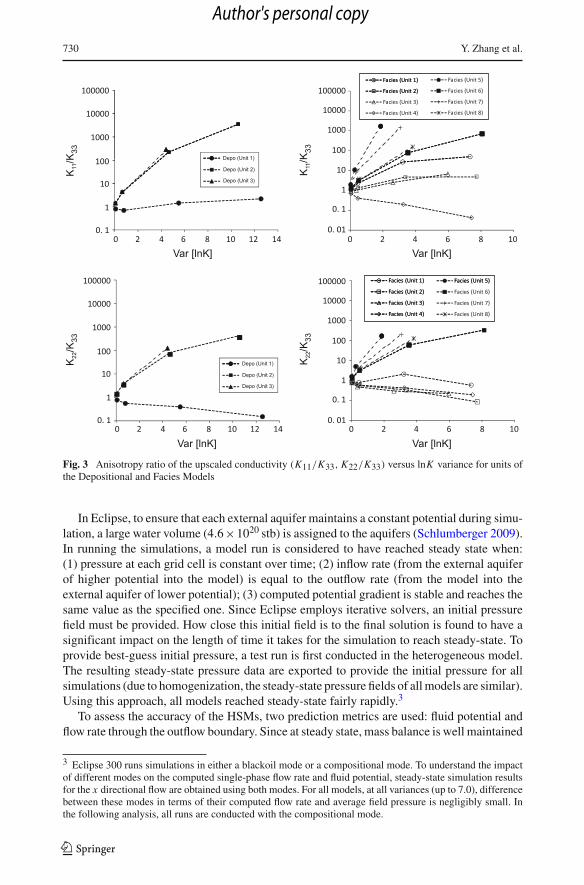
Fig. 3 Anisotropy ratio of the upscaled conductivity (K11/K33, K22/K33) versus lnK variance for units ofthe Depositional and Facies Models
In Eclipse, to ensure that each external aquifer maintains a constant potential during simu-lation, a large water volume (4.6×10²⁰ stb) is assigned to the aquifers (Schlumberger 2009).In running the simulations, a model run is considered to have reached steady state when:(1) pressure at each grid cell is constant over time; (2) inflow rate (from the external aquiferof higher potential into the model) is equal to the outflow rate (from the model into theexternal aquifer of lower potential); (3) computed potential gradient is stable and reaches thesame value as the specified one. Since Eclipse employs iterative solvers, an initial pressurefield must be provided. How close this initial field is to the final solution is found to have asignificant impact on the length of time it takes for the simulation to reach steady-state. Toprovide best-guess initial pressure, a test run is first conducted in the heterogeneous model.The resulting steady-state pressure data are exported to provide the initial pressure for allsimulations (due to homogenization, the steady-state pressure fields of all models are similar).Using this approach, all models reached steady-state fairly rapidly.3
To assess the accuracy of the HSMs, two prediction metrics are used: fluid potential andflow rate through the outflow boundary. Since at steady state, mass balance is well maintained
3 Eclipse 300 runs simulations in either a blackoil mode or a compositional mode. To understand the impactof different modes on the computed single-phase flow rate and fluid potential, steady-state simulation resultsfor the x directional flow are obtained using both modes. For all models, at all variances (up to 7.0), differencebetween these modes in terms of their computed flow rate and average field pressure is negligibly small. Inthe following analysis, all runs are conducted with the compositional mode.
123
Author's personal copy

Homogenization of Hydraulic Conductivity 731
(e.g., difference between inflow and outflow rates is typically less than 0.01 stb/day), onlythe outflow rate is used. In the following subsections, each prediction metric is presented.Impact of variance on the accuracy of the HSMs is discussed. Diagonal tensor approximationis also discussed.
3.2.1 Fluid Potential
Using results from all models, an absolute potential deviation (APD) can be computed foreach grid cell of the HSM: APD=|ΦHSM − Φref |, Φref is prediction by the heterogeneous(or reference) model. For each HSM, APD on the top surface of the grid is shown, onefor each flow direction (x-flow, y-flow, and z-flow) (Fig. 4; σ 2
f = 1.0). For each HSM (onecolumn), the pattern of APD is distinctly different from one another when flow directionvaries. When flow occurs in the same direction (one row), all HSMs display similar APDpatterns. APD is then checked layer by layer. Again, similar patterns persist among the HSMswhenever the boundary condition is the same. At this variance level, spatial distribution ofAPD appears sensitive to the boundary condition, but not to the homogenization level. Sameresult is observed for the low and high variance cases (not shown). However, in the highvariance case, though the APD pattern remains insensitive with the homogenization level,along any flow direction, magnitude of APD increases significantly with variance. Clearly,variance level is important to the accuracy of flow prediction.
When flow is lateral (x or y), APD map of a given HSM changes only slightly in thevertical direction. The map at the top surface closely resembles those at the other layers. Ata given layer, APD is observed to be relatively small near the inflow and outflow boundaries,but becomes larger in the central areas (Fig. 4). Thus, when flow is parallel to stratification,higher accuracy in fluid potential prediction appears to be associated with the two sides wherefluid potentials are fixed. The same result is observed when the system is at the lower andhigher variance levels, i.e., the same APD pattern persisting in the vertical direction andhigher accuracy near inflow/outflow boundaries. Clearly, variance has little influence on thepattern of APD.
When flow is vertical (perpendicular to stratification), the APD pattern on the top sur-face reflects the heterogeneity pattern at this location. For example, a lateral (along-x) APDzone exists, corresponding to the location of a high-K channel (Fig. 1). The APD also variessignificantly in the vertical direction, i.e., the surface feature no longer persists with depth.After layer-by-layer inspection, the APD pattern now reflects the geologic structure at thelayer depth. This result is also observed when the system is at lower and higher variances.Thus, when flow is perpendicular to stratification, APD pattern is dominated by geologicalstructure while variance impacts the accuracy (as discussed above).
To compare the accuracy of fluid potential prediction among experiments (i.e., differentboundary conditions), a global mean error (ME) in fluid potential is calculated:
ME = 1
n
n∑i=1
|ΦHSM − Φref | = 1
n
n∑i=1
APD (10)
where n is the number of grid cells. ME is normalized by the absolute potential drop acrossthe model in each experiment to compute a dimensionless mean relative error (MRE). MREis an unbiased indicator of the relative deviation in predicting fluid potential (Zhang et al.2006). For a given HSM, MRE can be used to compare among experiments. Results suggestthat for each HSM, MRE in predicting the fluid potential is consistently the largest when theflow is along the y direction (Fig. 5).
123
Author's personal copy

732 Y. Zhang et al.
Fig. 4 Absolute potential deviation visualized at the top model layer for each HSM (system lnK varianceis 1.0). From top to bottom: x-flow, y-flow, and z-flow, respectively; from left to right: 1-Unit, 3-Unit, and8-Unit, respectively
For a given HSM, when the magnitude of MRE is examined against variance, MREincreases with variance, for all flow directions (Fig. 5). At the variance of 0.1, MRE of allmodels ranges from 0.18% to 2.70%; at 1.0, 0.78% to 8.60%; at 7.0, 3.9% to 14.0%. Thissuggests that regardless of the type of the upscaled model used, fluid potential predictionbecomes less accurate when variance increases. Further, no single HSM appears to be con-sistently the most accurate, when all flow directions and all variances are considered. Forexample, for x-flow, the 8-unit model is always the most accurate; for y-flow, no model isconsistently the most accurate; for z-flow, the 1-unit model is the most accurate. In sum-mary, boundary condition, heterogeneity variance, and homogenization level all impact theaccuracy of the HSMs in predicting fluid potential.
3.2.2 Flow Rate
Table 4 presents the outflow rate computed by all models, for a variance up to 7.0. Figure 6presents the flow rate prediction error by the HSMs. Results suggest: (1) along a given flowdirection, prediction error in flow rate increases with variance, with one minor exception for
123
Author's personal copy

Homogenization of Hydraulic Conductivity 733
Fig. 5 Global MRE of the fluid potential predicted by the HSMs
y-flow (i.e., 3-unit model when σ 2f = 1.0). When σ 2
f ≤ 1.0, error in flow rate is around 1%
or smaller. When σ 2f = 7.0, error ranges from 7.2% to 31.6% for x-flow, 5.6% to 11.1% for
y-flow, and 6.9% to 20.6% for z-flow. (2) Along a given flow direction, error also increaseswith the level of homogenization (from the 8-unit to the 1-unit models), with the same minorexception as noted above. (3) At all variances, prediction accuracy is generally the highestfor y-flow, then z-flow, and x-flow. This is opposite of that found for MRE in fluid potentialprediction where y-flow yields the highest MRE. This discrepancy is not uncommon, how-ever, as past work indicates that the accuracy in fluid potential prediction does not alwayscorrespond to the accuracy in flow rate prediction.
123
Author's personal copy

734 Y. Zhang et al.
Table 4 Outflow rate predicted by all models. Based on results of the heterogeneous model (“Ref”),a relative error in flow rate prediction is computed for the HSMs
Variance of lnK Models x-flow y-flow z-flow
q (stb/day) (Errror/ref) % q (stb/day) (Errror/ref) % q (stb/day) (Errror/ref) %
0.1 Ref 17.214 − 16.904 − 11.458 −8-Unit 17.214 0.000 16.888 −0.095 11.460 0.017
3-Unit 17.231 0.099 16.885 −0.112 11.461 0.026
1-Unit 17.240 0.151 16.898 −0.035 11.465 0.061
1 Ref 24.249 20.736 11.314
8-Unit 24.352 0.425 20.758 0.106 11.357 0.380
3-Unit 24.678 1.769 20.735 −0.005 11.362 0.424
1-Unit 24.792 2.239 20.871 0.651 11.425 0.981
7 Ref 94.442 57.227 9.480
8-Unit 101.258 7.217 60.410 5.562 10.134 6.899
3-Unit 117.752 24.682 60.229 5.246 10.192 7.511
1-Unit 124.329 31.646 63.604 11.143 11.431 20.580
Fig. 6 Error in flow rate prediction by the HSMs. |Err| of Table 4 is plotted
Performance of the HSMs and the associated accuracy of the upscaled K∗ could be im-proved if the model sub-domains are alternatively defined. This, however, does not mean thatmore subdivisions are necessarily the better. Under certain conditions (e.g., x-flow) (Fig. 6),division of the 3-unit model into eight units significantly enhances the accuracy in flow rate
123
Author's personal copy

Homogenization of Hydraulic Conductivity 735
prediction; under other conditions (e.g., z-flow), subdivision does not enhance this accuracy.Still under other conditions (noted above for y-flow at low variance), non-linear effects mayoccur.
For the models investigated here, which homogenization level is optimal for fluid potentialor flow rate prediction depends on boundary condition and variance. In this study, the map-ping used to define the sub-domains is based on kriging which can only provide descriptionsof smoothed contacts, and sharp changes in material properties cannot be captured well.This limitation may have contributed to some aspects of the errors. Future work will con-sider using alternative approaches (e.g., percolation or connectivity analysis) to define theupscaling domains.
3.2.3 Diagonal Approximation
For efficiency, many flow simulators approximate conductivity full tensor with diagonal ten-sor. Frequently, full tensor information is either difficult to obtain, or if such informationis available, it is more convenient to rotate the model coordinate axes to be aligned withthe dominant K anisotropy axes. This approach, however, will not work well when differ-ent model sub-regions have different anisotropy directions. For the HSMs, errors in fluidpotential and flow rate predictions are assessed when diagonal tensors (listed in Table 2) areused. Single-phase verification tests are again conducted, with flow along the x direction(results for y-flow and z-flow are expected to be similar).4 For the models of this study,diagonal tensor approximation appears to give sufficiently accurate results in predicting bothfluid potential and flow rate. This observation holds true at variance levels up to 7.0. Futurework will assess other heterogeneities with significant dip angles.
3.3 Analytical Predictions
For the HSM units, principal components of the upscaled conductivity are compared to thosepredicted by analytical methods. Increasing variances are evaluated. Since theory by Gelhar(1993), as implemented in Eq. 7, is strictly valid for low variances, its predictions are madefor σ 2
f = 0.1 and 1.0 only. The high-variance version of Eq. 7 is also tested against the up-scaling results and is found inaccurate at higher variances. For the four non-positive-definitecases, the horizontal components are compared to the analytical predictions.
Results suggest: (1) with a few exceptions, all analytical methods are nearly equally accu-rate in capturing the principal components when the variance is low, i.e., σ 2
f ≤ 1.0; (2) inestimating K11 and K22, formulations proposed by Desbarats (1992) (Eq. 5) and Noetingerand Haas (1996) (Eq. 6) are consistently the most accurate at all variances;5 (3) most analyt-ical methods fail to capture K33 when variance is high. This suggests that estimation of theconductivity anisotropy ratio using analytical methods could be problematic. However, forthose few cases that analytical methods do capture K33, formulations of Desbarats (1992)and Noetinger and Haas (1996) are again the most accurate.
Analytical expressions of Desbarats (1992) and Noetinger and Haas (1996) are developedfor multiGaussian media at low variances. Herein, their accuracy is also demonstrated onnon-multiGaussian media while a full range of variance is tested. Since both formulations
4 To understand the impact of different simulator modules, diagonal-tensor simulations are conducted withEclipse 300 compositional mode, Eclipse 300 blackoil mode, and Eclipse 100. Different modules give con-sistent results.5 Results based on Eq. 6 vary from those of Eq. 5 by less than 1%. These two formulations are consideredidentical for the range of conductivity tested here.
123
Author's personal copy
736 Y. Zhang et al.
are based on power averaging, this suggests that power law may be a reliable tool for predict-ing conductivities of irregular deposits. However, models of this study have univariate andbivariate characteristics that closely match the requirements of the analytical methods. Thedensity function of lnK is unimodal, while the upscaling domains are large compared to thelnK integral scales (Table 1), satisfying theory requirement of an ergodic field for upscaling.Future work will evaluate the upscaling characteristics of deposits with multimodal densitiesas well as those that do not satisfy ergodicity.
4 Summary and Conclusion
Based on a synthetic aquifer exhibiting non-stationary, statistically anisotropic conductivitycorrelation, three HSMs are created: a Full Aquifer Model with a single unit, a DepositionalModel with 3 units, and a Facies Model with 8 units. These models are hierarchical, reflect-ing a non-unique division of space and different heterogeneity homogenization levels. Ageostatistical analysis of lnK is first conducted for the HSM units. Univariate and bivariateparameters such as mean and variance of lnK and directional integral scales are estimated.For these units, K is upscaled using numerical and analytical methods, for increasing lnKvariances. Impact of variance on the accuracy of the upscaled conductivity and associatedperformance of the HSMs is assessed. Results are summarized as follows:
(1) the numerical method is capable of upscaling irregular domains with reasonable accu-racy for a variance up to 7.0. For the models investigated, equivalent conductivity princi-pal components at different scales are related by weighted arithmetic means. Given theexistence of geometric connectivity, increasing variance can result in flow channelingin the lateral direction and increasing lateral:vertical anisotropy ratios of the equivalentconductivities.
(2) Accuracy of the upscaled conductivity and associated performance of the HSMs aresensitive to homogenization level, lnK variance, and boundary condition. At a fixedhomogenization level and boundary condition, variance strongly influences the accu-racy of the HSMs in predicting fluid potential and flow rate. The HSMs are more accuratewhen variance is low.In fluid potential prediction, spatial pattern of the prediction error is sensitive to bound-ary condition, but insensitive to homogenization level and variance (magnitude of sucherror is sensitive to variance). In flow rate prediction, besides variance, performance ofthe HSMs is affected by boundary condition. Under some conditions, the 3-unit modelappears optimal; under other conditions, the 8-unit model provides the optimal accuracy.
(3) At variance up to 7.0, HSM simulations conducted with full-tensor K∗ versus diago-nalized forms reveal little difference in flow rate and fluid potential predictions. For theheterogeneity evaluated here, diagonal tensor appears a good approximation.
(4) When the variance is low (less than 1.0), all analytical methods are found to be nearlyequally accurate. However, when variance becomes higher, analytical methods gener-ally become less accurate.The current study conducts stratigraphic mapping to identify a set of hierarchical depos-its. Hydrostratigraphic models of increasing complexity are then created. Units of thesemodels, most are of irregular shape, are subjected to an upscaling analysis. Since a singlegrid is used by all models, numerical discretization error due to grid coarsening is notintroduced into the upscaled models. The upscaled conductivity can thus be comparedacross scales. These models will be used in a future optimization analysis to understand
123
Author's personal copy

Homogenization of Hydraulic Conductivity 737
the effect of model complexity on prediction uncertainty. Though grid coarsening is notevaluated, this topic will be pursued in future work.
Acknowledgment Funding for this study was provided by a NSF grant EAR-0838250 awarded to the firstauthor. We acknowledge the insightful comments of the anonymous reviewers.
References
Ababou, R.: Identification of effective conductivity tensor in randomly heterogeneous and stratified aquifers.In: Proceedings of the 5th Canadian/American Conference on Hydrogeology: Parameter Idenfiticationand Estimation for Aquifer and Reservoir Characterization, pp. 155–157 (1991)
Ababou, R.: Random porous media flow on large 3-D grids: numerics, performance and application to homog-enization. In: Wheeler, M.F. (ed.) Mathematics and its Applications: Environmental Studies—Math,Comput and Statistical Analysis, IMA vol 79, Chapter 1, pp. 1–25. Springer, New York (1996)
Desbarats, A.J.: Spatial averaging of hydraulic conductivity in three-dimensional heterogeneous porousmedia. Math. Geol. 24(3), 249–267 (1992)
Desbarats, A.J., Srivastava, R.M.: Geostatistical analysis of groundwater flow parameters in a simulatedaquifer. Water Resour. Res. 27(5), 687–698 (1991)
Deutsch, C.V.: Geostatistical Reservoir Modeling. pp. 376 Oxford University Press, NY, USA (2002)Durlofsky, L.J.: Upscaling and gridding of fine scale geological models for flow simulation. In: Proceedings
of the 8th International Forum on Reservoir Simulation. Stresa, Italy, 20–25 June 2005Gelhar, L.W.: Stochastic Subsurface Hydrology. Prentice Hall, Englewood Cliffs, NJ, USA (1993)Gelhar, L.W., Axness, C.L.: Three-dimensional stochastic analysis of macrodispersion in aquifers. Water
Resour. Res. 19(1), 161–180 (1983)Journel, A.G., Deutsch, C., Desbarats, A.J.: Power averaging for block effective permeability. SPE Paper
15128 (1986)Knudby, C., Carrera, J.: On the relationship between indicators of geostatistical, flow and transport connec-
tivity. Adv. Water Resour. 28(4), 405–421 (2005)Knudby, C., Carrera, J.: On the use of apparent hydrauilc diffusivity as an indicator of connectivity.
J. Hydrol. 329(3–4), 377–389 (2006)Milliken, W., Levy, M., Strebelle, S., Zhang, Y.: The effect of geologic parameters and uncertainties on
subsurface flow: deepwater depositional systems. SPE Paper 109950 (2007)Noetinger, B., Haas, A.: Permeability averaging for well tests in 3D stochastic reservoir models. SPE
J. 36653, 919–925 (1996)Renard, P., de Marsily, G.: Calculating equivalent permeability: a review. Adv. Water Resour. 20(5-6),
253–278 (1997)Ritzi, R.W., Allen-King, R.M.: Why did Sudicky (1986) find an exponential-like spatial correlation struc-
ture for hydraulic conductivity at the Borden research site? Water Resour. Res. (2007). doi:10.1029/2006WR004935
Sanchez-Vila, X., Girardi, J.P., Carrera, J.: A synthesis of approaches to upscaling of hydraulic conductivi-ties. Water Resour. Res 31(4), 867–882 (1995)
Sanchez-Vila, X., Carrera, J., Girardi, J.P.: Scale effects in transimissivity. J. Hydrol. 183(1-2), 1–22 (1996)Sanchez-Vila, X., Guadagnini, A., Carrera, J.: Representative hydraulic conductivities in saturated groundwa-
ter flow. Rev. Geophys. (2006). doi:10.1029/2005RG000169Schlumberger: ECLIPSE, Technical Description 2009.2. Schlumberger (2009)Wen, X.-H., Gómez-Hernández, J.: Upscaling hydraulic conductivities in heterogeneous media: an overview.
J. Hydrol. (1996). doi:10.1016/S0022-1694(96)80030-8Wen, X.H., Durlofsky, L.J., Edwards, M.G.: Use of border regions for improved permeability upscaling. Math.
Geol. 35(5), 521–547 (2003)Zhang, D.: Stochastic methods for flow in porous media, coping with uncertainties. Academic Press, San
Diego, CA (2002)Zhang, Y.: Hierarchical geostatistical analysis of an experimental stratigraphy. Math. Geosci. (2008). doi:10.
1007/s11004-008-9180-6Zhang, Y., Gable, C.W., Person, M.: Equivalent hydraulic conductivity of an experimental stratigraphy—
implications for basin-scale flow simulations. Water Resour. Res. (2006). doi:10.1029/2005WR004720Zhang, Y., Gable, C. W., Sheets, B.: Equivalent hydraulic conductivity of three-dimensional heterogeneous
porous media: an upscaling study based on an experimental stratigraphy. J. Hydrol. 388, 304–320 (2010).doi:10.1016/j.jhydrol.2010.05.009
123
Author's personal copy
Related Documents