Homework 4, Problem 3 The Allee Effect. Homework 4, Problem 4a The Ricker Model.

Homework 4, Problem 3The Allee Effect

Homework 4, Problem 4aThe Ricker Model

Homework 4, Problem 4aThe Beverton-Holt Model

The Chemostat

Group Model Building Exercise

The Chemostat

• An apparatus for the continuous culture of bacterial populations in a steady state.

• Nutrients are supplied continuously to the culture vessel.

• The cells in the vessel grow continuously on these nutrients.

• Residual nutrients and cells are removed from the vessel at the same rate by an overflow, thus maintaining the culture at a constant volume.

The Chemostat

QuickTime™ and aTIFF (Uncompressed) decompressor

are needed to see this picture.

Your Task

• Derive a mathematical model of bacteria growth in a chemostat

• Use the model to design the system so that – The flow rate will not be so great as to

wash out the entire culture– The nutrient replenishment is sufficiently

rapid so the culture is able to grow normally

Building The Model

• Variables

Nutrient Concentration C(t) mass/vol

in growth chamber

Bacteria Density N(t) #/vol

in growth chamber

Building The Model• Parameters

Stock Nutrient C0 mass/volConcentration

Volume of growth V vol.Chamber

Inflow/Outflow Rate F vol/time

Bacteria growth rate k 1/time Yield constant 1/ #/mass

Assumptions

• Growth chamber is well mixed– No spatial variations

• There is a single, growth limiting nutrient

• Bacteria growth rate depend on nutrient availability, that is k = k(C)

• Nutrient depletion occurs continuously as result of reproduction

The Model

€

dN

dt= k(C)N −

F

VN

€

dC

dt= −αk(C)N −

F

VC +

F

VC0

reproduction outflow

consumption outflow inflow

What Should k(C) Be?

• Last time, when deriving logistic growth, we assumed k(C) = C– Bacteria growth increases linearly with

nutrient concentration

• Jacques Monod found that following function provided the best fit to data for bacteria feeding on a single nutrient:

Monod Function

€

k(C) =rC

a+C

The Monod Function

• This growth function is monotonically increasing with limit r as C → infinity.

• The parameter r is the maximum growth rate

• The parameter a is called that half-saturation constant

C

r/2

r

a

€

k(C) =rC

a+C

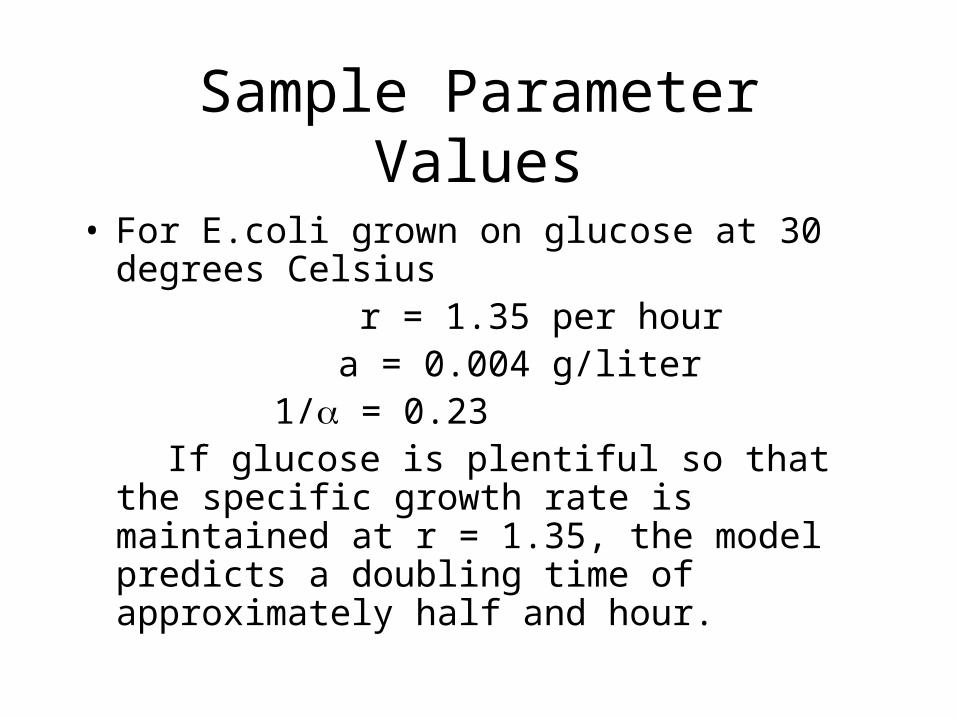
Sample Parameter Values

• For E.coli grown on glucose at 30 degrees Celsius

r = 1.35 per hour a = 0.004 g/liter 1/ = 0.23 If glucose is plentiful so that the specific

growth rate is maintained at r = 1.35, the model predicts a doubling time of approximately half and hour.

Bacteria Growth Without Maintenance

• The steady state for the bacteria depends on the initial conditions.

€

dN

dt=rC

a+CN

€

dC

dt= −α

rC

a+CN

Back to the Chemostat

• d = F/V is the dilution rate (1/time)• If the chemostat were filled it would take 1/d hours

to empty it. For this reason, 1/d is the mean residence time of bacteria cells in the chemostat

€

dN

dt=rC

a+CN − dN

€

dC

dt= −α

rC

a+CN − dC + dC0

Nondimensionalize

€

ATdn

dt=rBc

a+BcAn − dAn

€

BTdc

dt= −α

rBc

a+ BcAn − dBc + dC0

€

n =N

A

€

τ =Tt

Choose Arbitrary Scales:

Substitute in Model:

€

c =C

B

Nondimensionalize

€

dn

dt=r

T

ca

B+ cn −

d

Tn

€

dc

dt= −αAr

BT

ca

B+ cn −

d

Tc +dC0

BT

€

n =N

A

€

τ =Tt

Simplify€

c =C

B

Choices

€

T = r

€

T = d

€

B = a

€

B =dC0

T

€

A =BT

αr

Nondimensionalize

€

dn

dt=r

d

c

1+ cn − n

€

dc

dt= −

c

1+ cn − c +

C0

a

€

n =Nad

αr

€

τ =dt

€

c =C

a

Rename

€

a1 =r

d

€

a2 =C0

a

Only 2 parametergroupings governthe dynamics

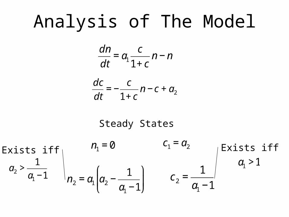
Analysis of The Model

€

dn

dt= a1

c

1+ cn − n

€

dc

dt= −

c

1+ cn − c + a2

Steady States

€

0 = a1

c

1+ cn − n

€

0 = −c

1+ cn − c + a2

€

€

n1 = 0

€

c1 = a2

€

n2 = a1 a2 −1

a1 −1

⎛

⎝ ⎜

⎞

⎠ ⎟

€

c2 =1

a1 −1

Analysis of The Model

€

dn

dt= a1

c

1+ cn − n

€

dc

dt= −

c

1+ cn − c + a2

Steady States

€

n1 = 0

€

c1 = a2

€

n2 = a1 a2 −1

a1 −1

⎛

⎝ ⎜

⎞

⎠ ⎟

€

c2 =1

a1 −1

Exists iff

€

a1 >1Exists iff

€

a2 >1

a1 −1

Stability

€

a11 =∂f

∂x(ne,ce )

€

a12 =∂f

∂y(ne,ce )

€

a21 =∂g

∂x(ne,ce )

€

a22 =∂g

∂y(ne,ce )

€

f (n,c) = a1

c

1+ cn − n

€

g(n,c) = −c

1+ cn − c + a2Let

Compute

€

λ1,2 =β ± β 2 − 4γ

2€

β =a11 + a22

€

γ=a11a22 − a12a21Let

Stability of Continuous Models

• In a continuous model, a steady state will be stable provided that eigenvalues are both negative (if real) or have negative real part (if complex).

• As with discrete models complex eigenvalues are associated with oscillatory solutions.

Necessary and Sufficient Conditions

• For a system of two equations, a steady state will be stable if:

€

β =a11 + a22 < 0

€

γ=a11a22 − a12a21 > 0

Stability of Chemostat

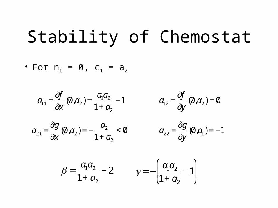
• For n1 = 0, c1 = a2

€

a11 =∂f

∂x(0,a2) =

a1a2

1+ a2

−1

€

a12 =∂f

∂y(0,a2) = 0

€

a21 =∂g

∂x(0,a2) = −

a2

1+ a2

< 0

€

a22 =∂g

∂y(0,a1) = −1

€

β =a1a2

1+ a2

− 2

€

γ=−a1a2

1+ a2

−1 ⎛

⎝ ⎜

⎞

⎠ ⎟

Stability of Chemostat• For n1 = 0, c1 = a2

€

β =a1a2

1+ a2

− 2 < 0

€

γ=−a1a2

1+ a2

−1 ⎛

⎝ ⎜

⎞

⎠ ⎟> 0

> 0 if:

€

a2 <1

1− a1

,a1 <1

So the elimination state is stable whenever the nontrivialsteady state does not exist.

< 0 if > 0

? ?

Stability of the Chemostat

• For n2, c2

€

a11 =∂f

∂x(n2,c2) = 0

€

a12 =∂f

∂y(n2,c2) =

a1n2

(1+ c2)2> 0

€

a21 =∂g

∂x(0,a2) = −

1

a1

< 0

€

a22 =∂g

∂y(0,a1) = −

n2

(1+ c2)2−1 < 0

€

β =−n2

(1+ c2)2+1

⎛

⎝ ⎜

⎞

⎠ ⎟< 0

€

γ= n2

(1+ c2)2> 0

Therefore the nontrivial steady state is stable whenever it exists.

Stability of the Chemostat

• Check for oscillations:

€

β =−n2

(1+ c2)2+1

⎛

⎝ ⎜

⎞

⎠ ⎟< 0

€

γ= n2

(1+ c2)2> 0

Therefore no oscillations are possible.

€

λ1,2 =β ± β 2 − 4γ

2

€

β 2 − 4γ < 0?

€

β 2 − 4γ =n2

(1+ c2)2+1

⎛

⎝ ⎜

⎞

⎠ ⎟

2

− 4n2

(1+ c2)2

⎛

⎝ ⎜

⎞

⎠ ⎟=

n2

(1+ c2)2−1

⎛

⎝ ⎜

⎞

⎠ ⎟

2

> 0

Is

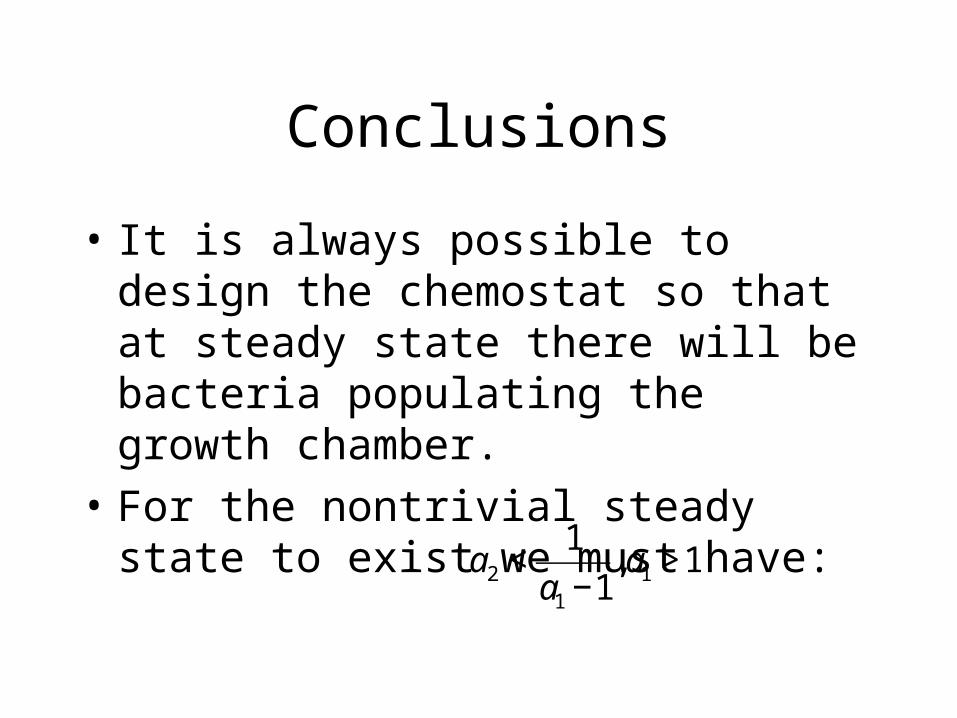
Conclusions

• It is always possible to design the chemostat so that at steady state there will be bacteria populating the growth chamber.

• For the nontrivial steady state to exist we must have:

€

a2 <1

a1 −1,a1 >1

Interpretation

What do these results mean in term of the original parameters?

That is what should the flow rate, the volume, and the stock nutrient concentration be in order to ensure continuous culture?

This is part of HW 5

Phase Portraits

• A graphical picture that summaries the behavior of a system of two ODEs.

• Example

€

dx

dt= xy − y

€

dy

dt= xy − x

Nullclines

• Nullclines are curves of zero slope– That is curves for which

– Therefore steady states are located at the intersection nullclines

€

dx

dt= 0 and

€

dy

dt= 0

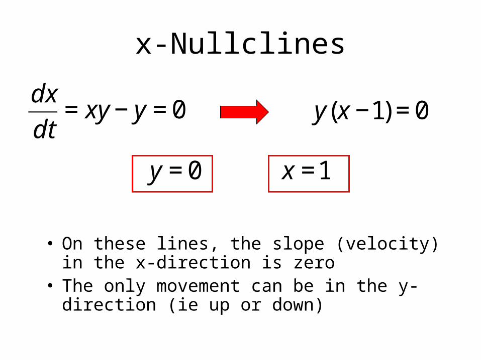
x-Nullclines

• On these lines, the slope (velocity) in the x-direction is zero

• The only movement can be in the y-direction (ie up or down)

€

dx

dt= xy − y = 0

€

y(x −1) = 0

€

y = 0

€

x =1

y-Nullclines

• On these curves, the slope (velocity) in the y-direction is zero

• The only movement can be in the x-direction (ie left or right)

€

dy

dt= xy − x = 0

€

x(y −1) = 0

€

x = 0

€

y =1

Graph the Nullclines

• Label the Steady States• Mark the Direction of Motion

x

y

1

1

€

x = 0

€

y =1

€

y = 0

€

x =1

x-nullclines

y-nullclines

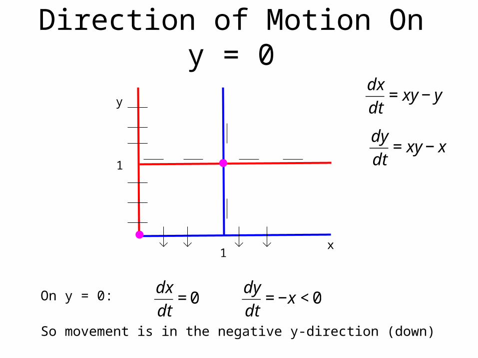
Direction of Motion On y = 0

On y = 0:

So movement is in the negative y-direction (down)

x

y

1

1

€

dx

dt= 0

€

dy

dt= −x < 0

€

dy

dt= xy − x

€

dx

dt= xy − y

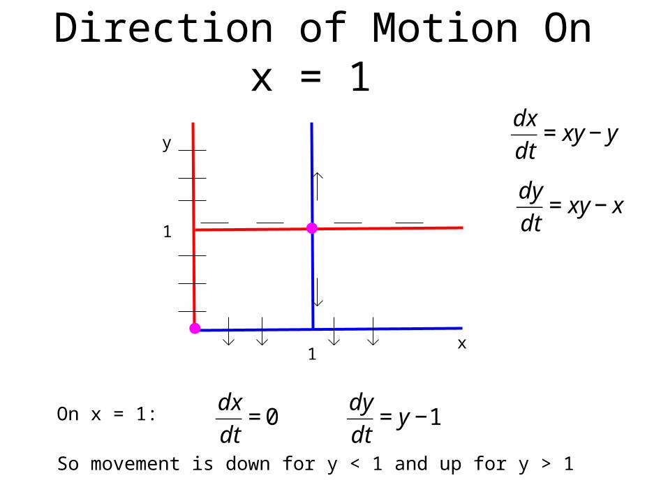
Direction of Motion On x = 1

On x = 1:

So movement is down for y < 1 and up for y > 1

x

y

1

1

€

dx

dt= 0

€

dy

dt= y −1

€

dy

dt= xy − x

€

dx

dt= xy − y

Direction of Motion On x = 0

On x = 0:

So movement is in the negative x-direction (left)

x

y

1

1

€

dx

dt= −y

€

dy

dt= 0

€

dy

dt= xy − x

€

dx

dt= xy − y

Direction of Motion On y = 1

On y = 1:

So movement is left for x < 1 and right for x > 1

x

y

1

1

€

dx

dt= x −1

€

dy

dt= 0

€

dy

dt= xy − x

€

dx

dt= xy − y

Fill in the Direction Field

All trajectories move away from the non-trivial steady state, thereforex = 1, y = 1 is unstable.Some trajectories move towards the origin, but some move away; therefore x = 0, y=0 is unstable.Note that arrows change direction across a steady state.

x

y

1

1

€

dy

dt= xy − x

€

dx

dt= xy − y

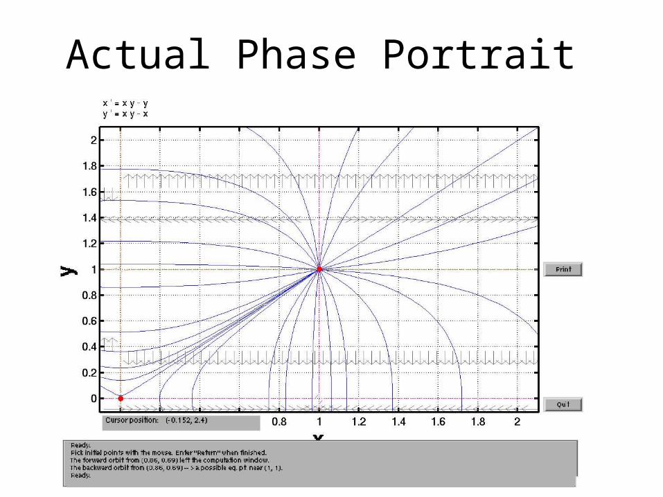
Actual Phase Portrait

Another Example

• Determine nullclines

– x-nullclines: • On this curve, slope (velocity) in the x-direction is zero• Trajectories can only move off of this curve in the y-direction (up or down)

– y-nullclines:• On this curve, slope (velocity) in the x-direction is zero• Trajectories can only move off of this curve in the y-direction (up or down)

€

dy

dt= x − y

€

dx

dt= x 2 − y

€

y = x 2

€

y = x

Graph the Nullclines

• Plot nullclines, label steady states, mark direction of motion

€

dy

dt= x − y

€

dx

dt= x 2 − y

€

y = x 2

€

y = x

x

y

1

1

x-nullclines

y-nullclines

Direction of Motion On y = x

On y = x:

So movement is left if x < 1 and right if x > 1

€

dy

dt= x − y

€

dx

dt= x 2 − y

€

y = x 2

€

y = x

x

y

1

1

€

dy

dt= 0

€

dx

dt= x 2 − x = x(x −1)

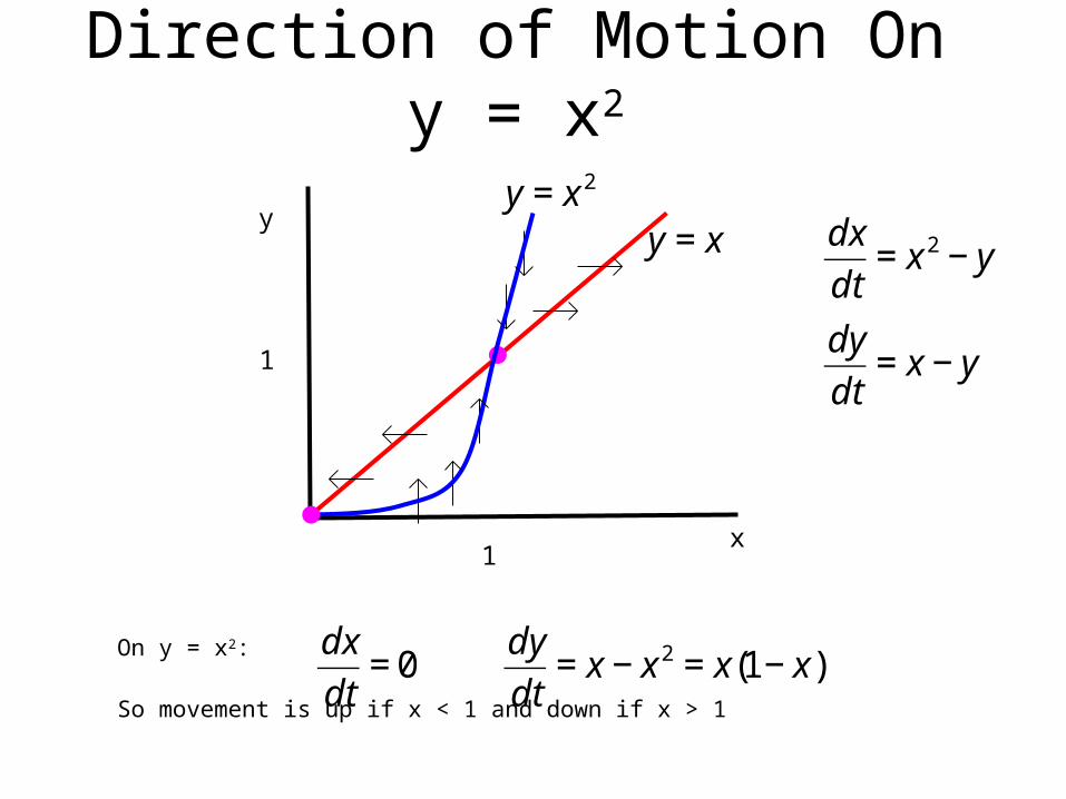
Direction of Motion On y = x2

On y = x2:

So movement is up if x < 1 and down if x > 1

€

dy

dt= x − y

€

dx

dt= x 2 − y

€

y = x 2

€

y = x

x

y

1

1

€

dx

dt= 0

€

dy

dt= x − x 2 = x(1− x)

Fill in the Direction Field

Some trajectories move towards the nontrivial steady state, but others move away; therefore x = 1, y = 1 is unstable.Trajectories seem to move toward the origin, therefore the origin could be stable.Note that arrows change direction across a steady state.

€

dy

dt= x − y

€

dx

dt= x 2 − y

€

y = x 2

€

y = x

x

y

1

1

Actual Phase Portrait

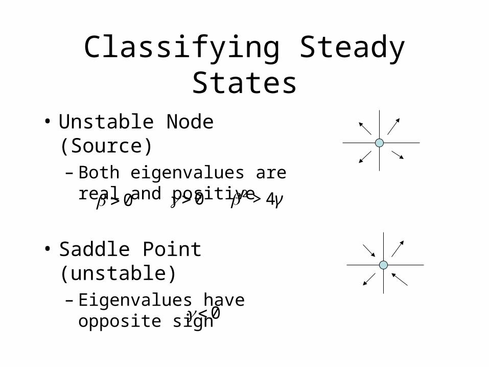
Classifying Steady States

• Unstable Node (Source)– Both eigenvalues are real

and positive

• Saddle Point (unstable)– Eigenvalues have opposite

sign€

γ> 0

€

β > 0

€

β 2 > 4γ

€

γ< 0

Classifying Steady States

• Unstable Spiral (Source)– Complex eigenvalues with

positive real part

• Neutral Center– Complex eigenvalues with zero

real part€

β > 0

€

β 2 < 4γ

€

β =0

€

β 2 < 4γ

Classifying Steady States

• Stable Spiral (Sink)– Complex eigenvalues with

negative real part

• Stable Node (Sink)– Eigenvalues are real and

negative€

β < 0

€

β 2 < 4γ

€

β < 0

€

γ> 0

Summary

• The local stability properties of steady states of a nonlinear system of two equations can be ascertained by determining b and g and noting the region of parameter space in which they lie.

€

λ1,2 =β ± β 2 − 4γ

2

€

β 2 − 4γ

€

β

€

γ

Global Behavior From Local Information

• For systems of 2 equations, local stability properties of steady states can be used to determine global behavior.

• There are a limited number of ways that trajectories can flow in the phase plane (due to continuity)

Properties of Trajectories in the Phase Plane

• Solution curves can only intersect at steady states

• If a solution curve is a closed loop, it must enclose at least one steady state.– That steady state cannot be a saddle point

Asymptotic Behavior of Trajectories

• Trajectories in the phase plane can– Approach a steady steady– Approach infinity– Approach a closed loop (a limit cycle)

• A trajectory itself may be a closed loop or else it may approach or recede from one

– Be a heteroclinic trajectory• Connects two different steady states

– Be a homoclinic trajectory• Returns to the the same steady state