Hog Production in China: Technological Bias and Factor Demand

Hog Production in China: Technological Bias and Factor Demand*

Hengyun Ma and Allan Rae

China Agriculture Working Paper 2/04

Centre for Applied Economics and Policy Studies,

Massey University, Palmerston North

New Zealand

* Financial support from FRST grant IERX0301is gratefully acknowledged.

Hog Production in China: Technological Bias and Factor Demand

Abstract

China’s agricultural output has expanded rapidly since the economic reforms of the late 1970s, reflecting both productivity growth and mobilization of inputs. Over the same period, increased consumption of livestock products has been a feature of China’s food consumption. Widely different projections of China’s demand for feedgrains to feed its expanding livestock sector have motivated this research. Productivity growth is an important component of such projections, but past estimates have been controversial, few focus on livestock, and we are aware of none that examine technological bias in China’s livestock production. For example, does the nature of technical progress lead to increased or reduced use of feedgrains relative to other inputs? A feature of China’s livestock sector is rapid structural change towards larger and more commercial and intensive production systems. As specialization has developed over the last two decades, the share of backyard livestock production has declined and the shares of specialized households and commercial enterprises have increased. We measure technological change and biases for each of these structures so that this information can be eventually combined with that on structural change when making feedgrain demand projections. Our commodity focus in this paper is on hog production, which is the major consumer of feedgrains in China. We use a translog cost function and adjusted livestock data to estimate technological change and biases. Technical change has not been neutral, and the bias towards feedgrain-saving was found to be statistically significant. We also find that the demand for feedgrains is elastic with respect to its own price and that strong substitution relationships exist with respect to some other inputs. Thus input price changes are important, along with technological biases, in changing the feedgrain input shares to hog production.

2

Hog Production in China: Technological Bias and Factor Demand

Introduction

China’s economic growth is driving rapid change in food consumption patterns,

including increased consumption of livestock products, which in turn is fuelling

China’s derived demand for feedgrains. A current concern is whether China’s grain

output expansion will be able to match its growth in demand from livestock producers

(Huang et al., 1999; Rutherford, 1999; Rae and Hertel, 2000; Simpson and Li, 2001;

Ianchovichina and Martin, 2003; Huang and Rozelle, 2003; Nin et al., 2004).

Nowadays, the question seems very clear - the concern has shifted from a very

general “who will feed China” to a very specific “who will feed China’s animals”

(Brown, 1995; Fuller et al. 2002; Simpson, 1997). Since pigmeat is still the major

meat consumed in China, and hog production accounts for over 55% of total feed

consumption by China’s livestock (feedgrain equivalent, authors’ calculations) hogs

will be the focus of this paper.

Answering the above questions will require a better understanding of

technological change and factor input relationships for China’s livestock sector.

Considerable variation exists between published estimates of technological change in

China’s agriculture, and very few estimates exist for livestock let alone for different

types of animal. Nin et al. (2004) estimated 3.0 percent annual growth in hog output

per head over 1991-97, Nin et al. (2003) reported growth in total factor productivity

(TFP) of 1.8 percent per year over 1965-94 for the aggregate livestock sector (but

around 6.5 percent over 1980-94), and Ludena (2004) estimated TFP annual growth

for non-ruminants of 4.33 percent over 1990-2001. None of these studies tests for

possible biases in technical progress, yet knowledge of whether such change is

feed-saving, feed-using, or neutral seems critical for projecting China’s feedgrain

demands. Nor do these studies differentiate between different production structures,

but this seems important for two reasons. First, feed-gain conversion coefficients vary

from approximately 2.0 in the backyard hog sector to around 2.5 for specialized

household and commercial hog production units.1 Second, structural change the

reduced the share of backyard hog production in total hog output from more than 90

percent in the early 1980s to only 71 percent in 2001.

1 Averages for 1999-2001 from State Development Planning Commission, “The Compiled Materials of Costs and Returns of Agricultural products of China.”

3

It is clear that differing assumptions about technical change in China’s livestock

production have contributed to the substantial variation in past projections of China’s

grain trade (Fan and Agcaiili-Sombilla 1997; Zhou 2004). Given the importance of

China’s livestock economy and inaccuracies of past feed grain projections, there is an

urgent need to study China’s feed grain demand so that more accurate projections of

China’s future grain trade can be made, and policy-makers can formulate improved

sectoral policies. We believe our paper makes a contribution by presenting an

improved understanding of technological change and factor demand in China’s hog

sector.

The paper is organized as follows. The next section will introduce our empirical

approach to measuring technological change and factor bias, conducting various

hypothesis tests, and deriving factor demand parameters. We then describe our data

sources including a detailed discussion of how we constructed our hog production and

factor demand data. In section four, we document the estimated econometric results

and major findings. The conclusions and implications will be presented in the final

section.

Methodology

The translog cost function is a convenient specification of duality theory that has

been favoured in empirical studies and as the second order approximation, its

application allows ones to avoid the need to specify a particular production function

(Stratopoulos et al., 2000). Nor is it necessary to assume constant or equal elasticities

of substitution (Woodland, 1975). We use a truncated third-order Taylor expansion in

this study instead of the usual second-order format for two reasons (Stevenson, 1980).

First, it allows all coefficients estimated from cross-sectional data to change from

time period t to jt + . Second, the truncated third-order form allows us to specify

certain tests not addressed under the second-order formulation, such as price-induced

technological factor bias. The third-order Taylor series expansion in time and the

logged input price and output can normally be expressed as:

4

ittiyTN

ijtitijTN

jN

i

TTyyTtyT

tyyitiTN

ititiyN

i

jtitijN

jN

iTtyitiN

it

PYTPPT

TYTYT

YPTYP

PPTYPC

lnlnlnln21

21)(ln

21ln

)(ln21lnlnln

lnln21lnlnln)1(

111

22

211

1110*

ββ

βββ

βββ

βββββ

∑∑∑

∑∑

∑∑∑

===

==

===

++

+++

+++

++++=

where ln indicates the natural logarithm; C* is the equilibrium total cost; Pjt (Pit)

denotes the price of input j (i) at time T; Yt is the level of output in period t and T

denotes a time trend reflecting biased technical change. With the proper set of

restrictions on its parameters, equation (1) can therefore be used to approximate any

of the unknown cost and production functions. The symmetry restrictions

(2) jiij ββ = and jiTijT ββ = for all ji ≠

imply equality of the cross-derivatives. Linear homogeneity in prices (when all factor

prices double, the total cost has to double) implies:

(3) , 11 =∑ = iN

i β 0111 === ∑∑∑ === iTN

iiyN

iijN

j βββ

and , 0111 === ∑∑∑ === iyTN

iijTN

jijTN

i βββ Ni ,,1L= .

By Shephard’s lemma, a firm’s system of cost minimizing demand functions (the

conditional factor demands) can be obtained by differentiating the total cost function

with respect to input prices to obtain the following system of factor input share

equations:

(4) TYTYPTPS iTiyTtiyjtijTN

jjtijN

jiTit ββββββ +++++= ∑∑ == lnlnlnln 11*

Measures of Technological Bias

Stevenson (1980) proposed several measures for technological bias. Given

factor-input prices and other state of nature constraints, technological change would

permit the firm to produce the same level of output at a lower level of expenditure.

Thus, on the cost side of the production dual, the rate of technological progress (TC)

can be measured as:

5

ittiyTN

ijtitijTN

jN

i

TTyyTtyTitiTN

iT

ZPY

t

PYPP

TYYP

TCTC

lnlnlnln21

)(ln21lnln

ln)5(

111

21

,,

*

ββ

βββββ

∑∑∑

∑

===

=

++

++++=

∂∂

=

where Z is a vector of “state of nature” variables.

Technological change may be biased both with regard to the factor inputs and

with regard to the scale characteristics of the production process. With regard to

technical change and factor input bias, Hicks’ definition of neutrality implied no

change in factor proportions or factor cost shares as technology progressed. Given the

existence of technological change, the following factor-share derivative with respect

to time can be used to measure factor input bias (FBi):

(6) iTtiyTjtijTN

jZPY

iti YP

TS

FB βββ ++=∂∂

= ∑ = lnln1,,

*

Technological change is factor i-using if , factor i-saving if and

neutral if .

0>iFB 0<iFB

0=iFB

Technological change may also be biased with respect to the return-to-scale

characteristics of the production process and such a factor bias would alter the range

over which returns to scale of a given degree could be realized, possibly altering the

output level at which minimum average costs could be attained. The scale measure

( ) can be expressed as: cS

itiyTN

ityyTyTtyyitiyN

iyt

tZPc PTYTTYP

YC

S lnlnlnlnlnln

)7( 11

*

,ββββββ ∑∑ == +++++=

∂∂

=

where implies the existence of economies of scale; 1<cS 1=cS means constant

return to scale, and indicates diseconomies of scale. The measure of

technological scale bias ( ) is expressed as:

1>cS

cTS

(8) itiyTN

ityyTyTZPY

cc PY

TS

TS lnln 1,,

βββ ∑ =++=∂∂

=

Assuming the sign of is the same over the output range, implies that

minimum efficient firm size is increased;

cTS 0<cTS

0=cTS indicates no change in minimum

6

efficient firm size; and signals minimum efficient firm size can be attained

at a lower level of output.

0>cTS

The extent to which factor-share bias is induced by factor-price shifts is given by:

(9) ijTj

iti PT

SPIB β=

∂∂∂

=*2

where ijTβ is expected to be positive for ji ≠ and negative for ji = .

Hypothesis Tests

Placing restrictions on the parameters of equations (1) and (4) permits

econometric testing of several economic hypotheses (Allen and Urga, 1999; Atkinson

and Halvorsen, 1998) as follows:

Constant return to scale (CRS):

(10) 1=yβ , 0=iyβ , ; Ni ,,2,1 L= 0== yTyy ββ , 0== iyTyyT ββ .

No overall technological change in China’s livestock production:

(11) 0==== TTyTiTT ββββ , 0=== yyTiyTijT βββ , Ni ,,2,1 L= .

No factor-input bias:

(12) 0=iTβ , 0== iyTijT ββ , .,,2,1, Nji L=

No price-induced factor input bias:

(13) 0=ijTβ , .,,2,1, Nji L=

No scale bias:

(14) 0=== iyTyyTyT βββ , .,,2,1 Ni L=

No scale-induced factor-share scale bias:

(15) 0== iyTyyT ββ , .,,2,1 Ni L=

Homothetic production technology not subject to technical progress growth bias:

(16) 0=iyβ , 0=iyTβ , .,,2,1 Ni L= 0=yTβ .

Allen Partial Elasticities of Substitution (AES)

Important economic information can be obtained in the form of elasticities of

substitution and factor demand elasticities. There are two commonly used summary

measurements of price responsiveness - the Allen-Uzawa partial elasticities of

substitution ( ijσ ) and the price elasticities of demand ( ijη ). Following Uzawa (1962)

7

and Binswanger (1974a), these (long run) elasticities for the translog cost function are

measured as:

iallforS

jijiallforSiallforSSST

jijiallforSST

iiiii

jijij

iiiiiTiiii

jiijTijij

ση

σηββσ

ββσ

=

≠=−++=

≠++=

;,/)(

;,/)(1)17(22

where is the share of ith factor, iS ijσ are the elasticities of substitution between

factors i and j, iiη are the own-price elasticities of demand for factors and ijη are

the cross-partial elasticities of demand for factors. A positive AES between factors i

and j indicates that they are substitutes, while a negative AES implies that the factors i

and j are complementary.

Data and Variable Construction

Cross-section and time-series data sets will be pooled in this study. Because of

the number of datasets to be used, we will clarify the data sources and discuss how

these datasets were constructed.

Hog Production Cost

Hog production cost data were obtained from “The Compiled Materials of Costs

and Returns of Agricultural Products of China.” These costs and returns were

originally collected from surveys of individual farms, but were then aggregated to the

provincial and national levels prior to publication by the State Development Planning

Commission. The cost surveys provide not only detailed factor expenditure but also

factor consumption for feed (in grain equivalents), labour and animal purchases.

The cost survey provides cost information on a ‘per unit animal’ basis so that we

can derive total costs by multiplying cost per animal by total numbers of the relevant

hog category. Labour includes the farmer and family labour and hired labour. Animal

purchases are the costs of young animals for hog production. All other inputs to

production were aggregated into an ‘other’ input category, which includes

non-livestock capital and fodder.2 No quantity data were available for these inputs.

Therefore, we have to set fodder and equipment capital into one input group.

2 Note that this input cost comprised 11 percent capital and 55 percent fodder for backyard hog farms, 22 percent capital and 35 percent fodder for specialized household hog farms, and 31 percent capital and 12 percent fodder for commercial hog farms on average in 1996-2001.

8

The hog production systems in China are complex, and include traditional

backyards units, specialized households and commercial hog operations. The cost

survey provides detailed cost data for these three types of production structure. When

used in conjunction with the production structure estimates (see below), they allow

model estimation by production structure, which is potentially valuable given the

substantial variation in production technologies (such as feeding practices) across the

three structures combined with rapid structural change in the hog sector.

Factor Prices

Factor prices for feed grain equivalent, labour and animal purchases were directly

derived from the cost survey data as total expenditure divided by quantity. However,

for the ‘other’ input category the cost survey provided only values and not volumes.

Therefore we used a general price index of agricultural production inputs.

Livestock Output

Traditionally, hog production data has been obtained directly from official

statistical yearbooks. However, many concerns have arisen over the quality of China’s

official livestock statistics and therefore some data adjustments may be prudent (ERS,

1998; Fuller et al. 2000). Taking the advantage of the First National Agricultural

Census of China (NACO), Ma et al. (2004) made comprehensive adjustments to

supply and demand data for China’s major livestock commodities and we use that

source’s adjusted livestock production data sets. A brief description of the adjustment

procedures is given below but the reader is referred to Ma et al. (2004).

Hog Production Structure

China’s livestock sector is experiencing a rapid evolution in production practices

that involve traditional backyard, specialized households and commercial enterprises.

There also appears to be considerable differences in production methods over the

three farm types. For example, traditional backyards make full use of readily available

low cost feedstuffs, while specialized households and commercial enterprises feed

their animals more grain and protein meal, implying that the shift from traditional

backyard to specialized household and commercial enterprises in livestock production

will increase feed grains consumption (Fuller, Tuan and Wailes, 2002). Surry (1990)

has pointed out the importance of such disaggregation by type of production since

9

most econometrically-estimated demand relations for feed inputs have been estimated

at a very aggregate level so failing to take into account the wide diversity of

production practices.

We constructed share sheets by hog production structure in order to disaggregate

total factor inputs by farm type. While estimation of output shares for each year is

impossible due to data unavailability, there exist a great variety of data sources that

allowed us to construct share sheets by hog production structure for various time

periods. Such data sources included the NACO (detailed data for 1996), Animal

Husbandry Statistics:1949-1988 (which give a picture of livestock structure in the

1980s), Agricultural Statistical Yearbooks, Animal Husbandry Yearbooks and a wide

variety of other materials (e.g., annual reports, authority speeches and specific

livestock surveys and websites) which allow estimation of production share for

various years. When all these data were combined with 1996 values from the census,

many missing values still existed. On the assumption that declining backyard

production and increasing shares of specialized and commercial operations were

gradual processes over the data period, linear interpolations were made to estimate all

missing values.

Empirical Results

Estimating Procedure and Hypothesis Tests

The full dual system of the total cost function and cost share equations was

estimated using Zellner’s seemingly unrelated regression technique. One share

equation had to be dropped since only N-1 share equations are linearly independent

due to the homogeneity restriction. As symmetry and homogeneity in input price have

to be satisfied theoretically, we always impose these two restrictions into our

estimation.

First, the cost and factor-share functions incorporating only the restrictions of

symmetry (equation 2) and homogeneity (equation 3) were estimated. Results are

given in Table 1. Several restricted versions of the model were next estimated to test

the various joint hypotheses concerning the nature of technical change and production

scale (equations 10 - 16). Estimates of the restricted models are not presented here,

but all null hypotheses were rejected at the 5 percent level for the national aggregate

hog cost function and the backyard cost function. The null hypotheses of no scale bias,

no scale-induced factor bias and homothetic technology could not be rejected in the

10

case of specialized household farms, nor could the latter with respect to commercial

farms.

Technological Change and Scale Bias

Given our final choice of models, we can measure the extent of technological

progress and any associated factor or scale biases (Table 2). By fixing factor prices

and output at their average 1991-2001 levels, we can calculate technological change

year by year for national aggregated hog production and the three types of hog farms

using equation (5). On average over this period, the effect of technological change has

been to reduce production costs by 3.2 percent per year in the aggregate.

Technological change was a little faster in backyard production (3.3 percent) and

therefore somewhat slower on specialized (2.1 percent) and commercial operations

(2.3 percent). In each case technological advancement was more rapid than during the

previous decade.

Factor biases were estimated with equation (6) by allowing factor prices and

output to change over time. At the national aggregate level, the effect of technological

change over 1991-2001 was to reduce the feed cost share from its average value of

44.9 percent in 1991 to 32.0 percent (i.e. the feed share was reduced due to

technological bias on average by 1.3 per year), and to increase the cost shares of

labour from 13.0 percent to 14.4 percent (but this bias was not statistically significant),

of animal purchases from 24.1 percent to 28.4 percent, and ‘other’ inputs from 18.1

percent to 25.2 percent. Thus technical change has been significantly feed-saving over

this period, and a similar result was obtained with respect to the feed input for each of

the three production types. Figure 1 shows how the trends in technological biases

shifted sharply between the 1980 and the 1990s. The feed-saving and ‘other’

input-using biases were stronger on the commercial farms, where technological biases

over the 1990s resulted in an average 2.1 percent reduction in the feed cost share.

During the 1980s, technological change was feed-using only on the specialized

household structure.

Explanation of the ‘other’ input bias is not straightforward since the ‘other’ input

includes fodder, capital and other miscellaneous inputs (see footnote 2). However,

after identifying the major reason for the sharp reduction of ‘other’ category in total

cost, we may conclude that in the 1980s ‘other’ saving bias is due to a sharp reduction

of fodder share in total cost, which implies that it is fodder-saving technological bias

11

in the 1980s. For example, the total cost share of ‘other’ category reduced by 16

percent in the 1980s (from 37 percent in 1980 to 21 percent in 1990) on backyard

farms, and the total cost share of fodder reduced by 11 percent (from 23 percent in

1980 to 12 percent in 1990) on backyard farms. Therefore, it can be calculated that

fodder accounts for two thirds of the total cost share reduction of ‘other’ input

category. Likewise, of the 28 percent reduction of ‘other’ input share in total cost on

specialized household farms, more than 80 percent was due to reduction in the share

of the fodder input in the 1980s. In other words, technologies adopted during the

1980s may have emphasized increased use of feed grains, but during the 1990s

technological biases may have been towards increased use of capital as well as use of

fodder as a feedstuff. In contrast, ‘other’ input-using technical bias in the 1990s most

likely implies fodder-using technical bias. For example, of the 25 percent total cost

share increase in the 1990s, nearly 80 percent is due to the share increase of the

fodder input on back yard farms. While the total cost share of the ‘other’ input on

specialized household and commercial farms apparently reduced in the 1990s (the

former reduced by 7 percent and the latter reduced by 4 percent), their total cost

shares of the capital input either significantly increased or were maintained (e.g.,

capital share in total cost increased by 57 percent on commercial farms), which likely

indicates ‘other’ input-using technical bias in the 1990s to have been capital-using

technical bias.

Technological change is significantly biased towards labour-using technology on

backyard production units. This finding is consistent with the reality of livestock

production in China. For example, it can be a good compromise for backyard hog

farms to adopt feed-saving and labour-using technologies, and to save feed grain,

backyard hog farms feed hogs more fodder that most likely also requires more labour.

Turning to the animal input, its cost share has generally been increased through

technological change, but there are differences among hog farms. For instance, though

commercial hog farms tended to animal-saving technology (insignificantly), only

backyard hog farms appear to adopt animal-using technology. Although we are not

sure, it is possibly due in part to the fact that backyard hog farms have to buy piglets

from markets, but commercial hog farms have adopted their own breeding systems

and can be self-sufficient in piglet supply.

Scale elasticities are estimated from equation (7). Averaged over 1991-2001,

these elasticities were 1.013 for both backyard operations and at the national

12

aggregate level, and 1.074 for specialized households. The elasticities for individual

years showed a declining trend over the entire data period for backyard operations and

in the aggregate, indicating that technological change was biased towards increasing

the minimum efficient firm size. The opposite bias was found for specialized

households, where technological change had the effect of reducing the efficient firm

size over time. The scale elasticities were less than one each year for the commercial

farms, indicating economies of scale. However, technological change did not appear

to exert a scale bias on these farms.

Factor Demand and Substitution

All own-price elasticities of factor demand have the expected sign (table 3). In

general, feed and ‘other’ input demands are elastic, but labour and animal demands

are inelastic. Similar patterns are found across the three production structures. The

cross-price elasticities of Table 4 are positive for all but one factor pair (feed and

labour on specialized farms) indicating that factor substitution is the norm. The

highest cross-elasticities are those that measure a strong substitution effect between

feed and ‘other’ inputs. For example, a one percent increase in feed prices gives rise

to an increase in the demand for ‘other’ inputs of three and six percent depending on

farm type. The demand for feed is also elastic with respect to the ‘other’ input price.

We believe this captures substitution between feedgrain and fodder, given the

inclusion of the latter in the definition of the ‘other’ input.

The Allen partial substitution elasticities (Table 5) show considerable variation

across input pairs. All are positive at the national level, indicating substitution

relationships. The strongest substitution effects are found for the feed - ‘other’ and

labour – ‘other’ pairs of inputs. Given that the ‘other’ input category necessarily

aggregated feed in the form of fodder, and non-livestock capital, it is possible that

these estimates are picking up substitution between feed grain and fodder inputs on

the one hand, and between labour and capital on the other.

All but one of the substitution elasticities are also positive across the three farm

types. The exception is the apparent complementary relationship between feed and

labour on specialized hog farms, suggesting that increased feed use could help absorb

surplus rural labour. There are also some differences in the trend and magnitudes of

the labour and ‘other’ input substitution elasticities across farm types. For the

backyard hog farms, the elasticity averaged less than one over the 1990s but showed a

13

rising trend. For the specialized and commercial hog farms, this substitution

relationship was stronger on average over the 1990s but decreased sharply over the

last two decades in the case of commercial farms but displayed a rising trend on

specialized farms.

Conclusion and Implication

Our empirical results suggest that technological change had been more rapid in

the 1990s than the previous decade, in both the aggregate and on each farm type.

During both decades, the rate of change was greatest on backyard farms. We found

evidence of scale economies only on commercial farms, but no evidence that these

farms are using technologies that encourage larger-scale operations. But we found

evidences of significant scale diseconomies on specialized household farms.

The nature of innovation indicates the technological advancement over the 1990s

has generally been feedgrain-saving and using of all other inputs. At constant input

prices, this would imply that cost-minimizing hog farms producing a given level of

output would be induced by technological change to substitute labour, animal and

‘other’ inputs for feed grain. These results may go some way to explain why China

has recently been exporting, rather than importing corn. The annual changes in cost

shares resulting from these biases appear to have been significant, in particular for the

changes in cost shares of feedgrain and ‘other’ inputs. There are some exceptions to

this pattern of biases with respect to commercial farms (where animal and

labour-saving biases are found) but the estimated biases in these cases are not

significant.

The demand for feed and ‘other’ inputs appears very elastic with respect to

own-price, but labour and animal input demands are inelastic. Thus changes in the

relative prices of grain, fodder and farm capital could significantly affect their

demands (given the dominance of the latter two in the ‘other’ input category). While

rising feedgrain prices may produce a policy challenge through benefiting crop

farmers at the expense of hog farmers, the ease with which feedgrain can be

substituted with fodder will have an ameliorating effect. The highest partial

substitution elasticies were between the feed-‘other’ input pair. As regards the feeding

regime, this might imply that either feedgrain intensive or fodder extensive practices

could be chosen especially for backyard hog farms since a substantial proportion of

the ‘other’ input comprised fodder (an average of 55 for 1996-2001). Labour-‘other’

14

substitution was also relatively strong. This could measure labour-capital substitution

on commercial farms in particular, where the ‘other’ input included a large proportion

of capital expenditure (31 percent on average over 1996-2001. Further disaggregation

of the ‘other’ input into fodder and capital may help strengthen this conclusion. This

would appear to require new farm survey work.

Our research found some evidence of complementarity between feed and labour,

but only for specialized household hog farms. While the relevant partial substitution

elasticity was significantly different from zero (Table 5) the cross-price elasticities

(Table 4) were not. Thus while our statistical evidence is not compellingly strong, the

finding does suggest another area for further study. If confirmed, it could suggest that

encouragement of feed use could also provide more opportunities for labour

employment on hog farms.

Due to the reality that backyard hogs were fed with a lot of fodder and given

backyard hog farmers are price takers, this suggests there is strong substitution

between fodder and something else. Unfortunately, due to the unavailability of either

quantity or price data, we could not disaggregate the fodder input in the model.

Therefore, more work on fodder needs to be done so as to identify the substitution

relation between fodder and other inputs.

It should be noted that the model used in this study is still a traditional translog

cost approach. Therefore the relative influences of particular investments or policy

actions on technological change were not identified in this paper. In addition, using a

time trend to measure technical change is an implicit acknowledgment that at least the

dependent variable is nonstationary. Thus, dynamic specifications of this translog cost

function may be more appropriate for empirical estimation.

15

References:

1. Allen, C. and G. Urga. “Interrelated Factor Demands from Dynamic Cost Functions: An Application to the Non-Energy Business Sector of UK Economy.” Economica. 66(May 1999):403-413.

2. Atkinson, S. E. and R. Halvorsen. “Parametric Tests for Static and Dynamic Equilibrium.” Journal of Econometrics. 85(January 1998):33-55.

3. Binswanger, H. “The Measurement of Technical Change Biases with Many factors of Production.” The American Economic Review. 64(December 1974b):964-976.

4. Brown, L.R. “Who Will Feed China? Wake-Up Call For A Small Planet.” The World Watch Environmental Alert Series. First Edition, Published by World Watch Institute, 1995.

5. ERS [Economic Research Service]. “Statistical Revision Significantly Alter China’s Livestock PS&D.” Livestock and Poultry: World Market and Trade, Foreign Agricultural Service, U.S. Department of Agriculture. Circular Series FL&P 2-98 Oct. 1998.

6. Fan, S. and M. Agcaoili-Sombilla. “Why Projection on China's Future Food Supply and Demand Differ.” Australian Journal of Agricultural and Resource Economics. 41(June 1997):169-90.

7. Fuller, F., D. Hayes, and D. Smith. “Reconciling Chinese Meat Production and Consumption Data.” Economic Development and Cultural Change 49(2000):23-43.

8. Fuller, F., F. Tuan and E. Wailes. “Rising Demand for Meat: Who Will Feed China’s Hogs.” China’s Food and Agriculture: Issues for the 21st Century / AIB 775. Economic Research Service/USDA. 2002.

9. Fuller, F., F. Tuan and E. Wailes. “Rising Demand for Meat: Who Will Feed China’s Hogs.” China’s Food and Agriculture: Issues for the 21st Century / AIB 775. Economic Research Service/USDA. 2002.

10. Huang, J., S. Rozelle, and M. W. Rosegrant. "China’s Food Economy to the 21st Century: Supply, Demand and Trade.” Economic Development and Cultural Change. 47(July 1999):737-766.

11. Ianchovichina, E. and W. Martin. Economic impacts of China’s accession to the World Trade Organisation. Policy Research Working Paper 3053, World Bank, Washington D.C. 2003. Huang, J. and S. Rozelle. "Trade Reform, WTO and China’s Food Economy in the 21st Century." Pacific Economic Review. 8(June 2003):143-156.

12. Ludena, C. “Impact of productivity growth in crops and livestock on world food trade patterns”. Presented to 7th Annual Conference on Global Economic Analysis, Washington D.C., USA, 17-19 June 2004.

13. Ma, H., J. Huang and S. Rozelle. “Reassessing China’s Livestock Statistics: Analyzing the Discrepancies and Creating New Data Series.” Economic Development and Cultural Change. 52 (January 2004):445-473.

14. Ministry of Agriculture. Livestock Statistics of China, 1949-1988. Beijing: China Economy Press, 1990.

15. Ministry of Agriculture. Statistical Yearbooks of Agriculture of China. Beijing: China’s Statistical Press, 1981-2002 (annual).

16. Ministry of Agriculture. Statistical Yearbooks of Animal Husbandry of China. Beijing: China’s Statistical Press, 1999-2002 (annual).

17. NACO [National Agricultural Census Office]. The First National Agricultural Census Data Collection of China. Beijing: China Statistics Press, 1999.

16

18. Nin, A., C. Arndt, T.W. Hertel and P.V. Preckel. “Bridging the gap between partial and total productivcity measures using directional distance functions”. American Journal of Agricultural Economics 85(4): 928-42, 2003.

19. Nin, A., T.W.Hertel, K. Foster and A.N. Rae. “Productivity growth, catching-up and uncertainty in China’s meat trade”. Agricultural Economics 31(1): 1-16, 2004.

20. Rae A. N., and T. Hertel. “Future Development in Global Livestock and Grains Markets: The Impact of Livestock Productivity Convergence in Asian-Pacific.” The Australian Journal of Agricultural and Resource Economics. 44(September 2000):393-422.

21. Rutherford, A.S. Meat and milk self-sufficiency in Asia: Forecasts, trends and implications. Agricultural Economics 21(August 1999):21-39.

22. Simpson, J. R. “China’s Ability to Feed its Livestock in the Next Century.” Asia Pacific Journal of Economics and Business. 1(December 1997):69-84.

23. Simpson, J. R. and O. Li. “Long-Term Projections of China’s Supply and Demand of Animal Feedstuffs.” International Agricultural Trade Research Consortium, 18-19 January 2001, Auckland, New Zealand.

24. State Development Planning Commission. National Agricultural Production Cost and Return Collection. Beijing, 1980-2002 (annual).

25. Stevenson, R. “Measuring Technological Bias.” American Economic Review. 70(March 1980):162-173.

26. Stratopoulos, T., E. Charos and K. Chaston. “A Translog Estimation of the Average Cost Function of the Steel Industry with Financial Accounting Data.” International Advances in Economic Research. 6(May 2000):271-286.

27. Surry, Y. “Econometric Modeling of the European Community Compound Feed Sectors: An Application to France.” Journal of Agricultural Economics. 41(1990):404-421.

28. Uzawa, H. “Production Functions With Constant Elasticities of Substitution.” Review of Economic Studies. 29(October 1962):291-299.

29. Woodland, A. D. “Substitution of Structure, Equipment and Labor in Canadian Production.” International Economic Review. 16(February 1975):171-187.

30. Zhou, Zhangyue. “Feed versus Food: The Future Challenge and Balance for Farming.” Australian Agribusiness Review. 12(June 2004).

17

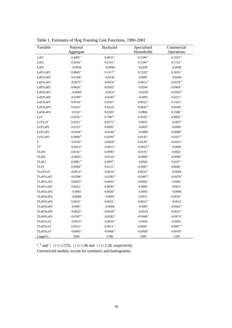
Table 1. Estimates of Hog Translog Cost Functions, 1980-2001

Variable National Aggregate

Backyard Specialised Households

Commercial Operations

LnP1 0.4405 a 0.4653 a 0.5290 a 0.5593 a

LnP2 0.2016 a 0.2161 a 0.1596 b 0.1722 a

LnP3 -0.0026 -0.0098 0.0259 -0.0658 LnP1LnP1 0.0845 a 0.1117 a 0.1320 a 0.2035 a

LnP1LnP2 -0.0168 c -0.0142 0.0087 -0.0204 LnP1LnP3 -0.0675 a -0.0676 a -0.0612 b -0.0570 b

LnP2LnP2 0.0626 a 0.0502 a 0.0244 0.0364 b

LnP2LnP3 -0.0068 -0.0115 -0.0239 -0.0383 b

LnP2LnP4 -0.0390 a -0.0245 b -0.0091 0.0223 c

LnP3LnP3 0.0518 a 0.0567 a 0.0832 b 0.1501 a

LnP3LnP4 0.0225 c 0.0224 c 0.0020 b -0.0548 c

LnP4LnP4 0.0167 0.0320 c 0.0866 0.1586 a

LnY 0.8331 a 0.7987 a 0.9556 a 0.9892 a

LnYLnY 0.0223 a 0.0272 a 0.0055 -0.0057 LnYLnP1 0.0123 a 0.0093 c -0.0037 0.0000 LnYLnP2 -0.0164 a -0.0146 a -0.0080 -0.0080 c

LnYLnP3 0.0099 b 0.0109 b 0.0143 c 0.0167 b

T -0.0542 a -0.0628 a 0.0238 c -0.0455 a

TT -0.0013 a -0.0012 a -0.0016 b -0.0005 TLnP1 0.0141 a 0.0096 a 0.0116 c 0.0032 TLnP2 -0.0093 a -0.0114 a -0.0068 c -0.0096 a

TLnP3 0.0081 b 0.0097 a 0.0066 0.0197 a

TLnY 0.0094 b 0.0121 a -0.0087 c 0.0066 c

TLnYLnY -0.0013 b -0.0016 a 0.0016 c -0.0004 TLnP1LnP1 -0.0296 a -0.0293 a -0.0407 a -0.0470 a

TLnP1LnP2 -0.0025 b -0.0033 a -0.0036 c 0.0001 TLnP1LnP3 0.0022 c 0.0030 a 0.0006 0.0015 TLnP2LnP2 -0.0001 0.0020 b 0.0003 -0.0006 TLnP2LnP3 -0.0006 -0.0001 0.0011 0.0016 c

TLnP2LnP4 0.0032 a 0.0015 c 0.0022 c -0.0012 TLnP3LnP3 0.0007 -0.0004 -0.0007 -0.0063 a

TLnP3LnP4 -0.0023 c -0.0026 b -0.0010 0.0032 c

TLnP4LnP4 -0.0307 a -0.0285 a -0.0449 a -0.0474 a

TLnP1LnY -0.0013 a -0.0010 a -0.0001 0.0003 TLnP2LnY 0.0013 a 0.0011 a 0.0006 c 0.0007 b

TLnP3LnY -0.0005 c -0.0006 b -0.0008 c -0.0018 a

Logged L 2940 2788 1369 1184

a, b and c: 2.576, 1.96 and 1.28, respectively. >|| t >|| t >|| tUnrestricted models, except for symmetry and homogeneity.

18

Table 2. Technological Change, Factor Input Bias, Scale Economies and Scale Bias Hog Farm Types 1980-1990 (S.E) 1991-2001 (S.E) Technical Change (TC):

National Aggregate -0.0185 (.0049)*** -0.0322 (.0045)***

Backyard Households -0.0195 (.0050)*** -0.0325 (.0047)***

Specialized Households -0.0042 (.0074) -0.0214 (.0061)***

Commercial Operations -0.0172 (.0082)** -0.0226 (.0065)***

Factor-Input Bias (FBi): Feed National Aggregate 0.0025 (.0014) -0.0129 (.0025)***

Backyard Households 0.0016 (.0015) -0.0128 (.0024)***

Specialized Households 0.0090 (.0021)*** -0.0180 (.0037)***

Commercial Operations 0.0028 (.0020) -0.0209 (.0042)***

Factor-Input Bias (FBi): Other National Aggregate -0.0083 (.0013)*** 0.0071 (.0024)***

Backyard Households -0.0068 (.0015)*** 0.0065 (.0024)***

Specialized Households -0.0110 (.0019)*** 0.0171 (.0035)***

Commercial Operations 0.0017 (.0019) 0.0256 (.0041)***

Factor-Input Bias (FBi): Labor National Aggregate 0.0019 (.0012) 0.0014 (.0013) Backyard Households 0.0033 (.0012)*** 0.0026 (.0013)**

Specialized Households 0.0006 (.0015) -0.0005 (.0019) Commercial Operations -0.0027 (.0012)** -0.0020 (.0015)

Factor-Input Bias (FBi): Animal National Aggregate 0.0039 (.0012)*** 0.0043 (.0013)***

Backyard Households 0.0036 (.0012)** 0.0038 (.0013)***

Specialized Households 0.0014 (.0016) 0.0014 (.0022) Commercial Operations -0.0017 (.0019) -0.0027 (.0024)

Scale Economies (Sc) b: National Aggregate 1.0305 (.0206) 1.0133 (.0202) Backyard Households 1.0403 (.0213) 1.0132 (.0201) Specialized Households 1.0191 (.0034)*** 1.0740 (.0254)***

Commercial Operations 0.9813 (.0329) 0.9860 (.0279) Scale Bias (TSc) c:

National Aggregate -0.0019 (.0020) -0.0022 (.0023) Backyard Households -0.0082 (.0021)*** -0.0031 (.0024) Specialized Households 0.0021 (.0030) 0.0029 (.0040) Commercial Operations 0.0015 (.0027) 0.0014 (.0039)

Note: Technical change was based on means of factor prices and output, while scale economies were based on means of factor prices over the relevant period. Factor bias and scale bias were calculated using actual prices and output levels since there is no time variable in their equations. a Standard errors are in parenthesis.b the null hypothesis of scale economies is Sc equal to one. c the null hypothesis of scale bias is TSc equal to zero. *** and ** stand for 1 percent and 5 percent significant levels, respectively.

19

Table 3. Own-Price Elasticities of Demand for Inputs for Hog Production (1991-2001)

Production Feed Labour Animal Other

National Aggregate

-1.4166

(.1627)

-0.4666

(.0618)

-0.4947

(.0447)

-3.8859

(.4688)

Backyard -1.4093

(.1749)

-0.3754

(.0575)

-0.5482

(.0450)

-3.4208

(.4524)

Specialized Households

-1.4462

(.1507)

-0.5616

(.1607)

-0.4658

(.0552)

-5.8484

(.6565)

Commercial Operation

-1.3904

(.1563)

-0.4777

(.1691)

-0.5487

(.0696)

-6.4890

(.8440)

Note: In parentheses are standard errors, which are estimated by: iiiTiiiiTiiii STTES /)],cov(2)var()[var()(. 5.02 ββββη ++=

20

Table 4. Cross-Partial Elasticities of Demand for Inputs in Hog Production (1991-2001)

Factor Feed Labor Animal Other

Aggregate: Feed -1.4166 (.1627) 0.0397 (.0213) 0.1577 (.0208) 1.2191 (.1604) Labour 0.1077 (.0576) -0.4666 (.0618) 0.1300 (.0455) 0.2288 (.0638) Animal 0.3088 (.0408) 0.0939 (.0329) -0.4947 (.0447) 0.0920 (.0435) Other 3.5078 (.4614) 0.2429 (.0678) 0.1352 (.0640) -3.8859 (.4688) Backyard: Feed -1.4093 (.1749) 0.0287 (.0216) 0.1773 (.0209) 1.2033 (.1716) Labour 0.0656 (.0493) -0.3754 (.0575) 0.1507 (.0403) 0.1590 (.0614) Animal 0.3405 (.0402) 0.1266 (.0339) -0.5482 (.0450) 0.0811 (.0468) Other 3.1301 (.4464) 0.1810 (.0699) 0.1098 (.0633) -3.4208 (.4524) Specialized: Feed -1.4462 (.1507) -0.0112 (.0232) 0.1647 (.0245) 1.2926 (.1513) Labour -0.0750 (.1553) -0.5616 (.1607) 0.1860 (.1211) 0.4506 (.1800) Animal 0.3341 (.0497) 0.0564 (.0367) -0.4658 (.0552) 0.0753 (.0506) Other 5.4109 (.6332) 0.2821 (.1127) 0.1554 (.1045) -5.8484 (.6565) Commercial: Feed -1.3904 (.1563) 0.0265 (.0177) 0.2055 (.0264) 1.1584 (.1541) Labour 0.2596 (.1733) -0.4777 (.1691) 0.0470 (.1588) 0.1711 (.2166) Animal 0.4456 (.0572) 0.0104 (.0352) -0.5487 (.0696) 0.0927 (.0577) Other 6.1683 (.8206) 0.0931 (.1178) 0.2276 (.1418) -6.4890 (.8440) Note: Each element in the table is the elasticity of demand for the input in the row after a price changeof the input in the column. These elasticities are not symmetric. In parentheses are standard errors, which are estimated by:

iijTijijTijij STTES /)],cov(2)var()[var()(. 5.02 ββββη ++=

21

Table 5. Elasticities of Substitution Between Pairs of Inputs for Hog Production, 1991-2001

Production Feed- Labour

Feed- Animal

Feed- Other

Labour- Animal

Labour- Other.

Animal- Other

National Aggregate

0.2399 (.0213)

0.6878 (.0208)

7.8130 (.1604)

0.5670 (.0455)

1.4665 (.0638)

0.5894 (.0435)

Backyard 0.1537 (.0216)

0.7977 (.0209)

7.3323 (.1716)

0.6781 (.0403)

0.9691 (.0614)

0.4940 (.0468)

Specialized Households

-0.1411 (.0232)

0.6286 (.0245)

10.1808 (.1513)

0.7098 (.1211)

3.5487 (.1800)

0.5929 (.0506)

Commercial Operation

0.4545 (.0177)

0.7803 (.0264)

10.8011 (.1541)

0.1785 (.1588)

1.5953 (.2166)

0.8645 (.0577)

Note: The elasticities of substitution are symmetric. Since the own elasticities of substitution have little economic meaning, we did not need to present them in this table (Binswanger, 1974b). In parenthesesare standard errors, which are estimated by:

jiijTijijTijij SSTTES /)],cov(2)var()[var()(. 5.02 ββββσ ++=

22

-0.025-0.020-0.015-0.010-0.0050.0000.0050.0100.0150.020

1980 1982 1984 1986 1988 1990 1992 1994 1996 1998 2000

Feed Labor Animal Others

Figure 1. Hog Production Input Biases at National Aggregate Level over time

23