History of Soil Geography in the Context of Scale - CORE

Agronomy Publications Agronomy

9-2015

History of Soil Geography in the Context of ScaleBradley Allen MillerIowa State University, [email protected]

R. J. SchaetzlMichigan State University

Follow this and additional works at: http://lib.dr.iastate.edu/agron_pubs

Part of the Agronomy and Crop Sciences Commons, and the Soil Science Commons

The complete bibliographic information for this item can be found at http://lib.dr.iastate.edu/agron_pubs/72. For information on how to cite this item, please visit http://lib.dr.iastate.edu/howtocite.html.

This Article is brought to you for free and open access by the Agronomy at Digital Repository @ Iowa State University. It has been accepted forinclusion in Agronomy Publications by an authorized administrator of Digital Repository @ Iowa State University. For more information, pleasecontact [email protected].

1

HISTORY OF SOIL GEOGRAPHY IN THE CONTEXT OF SCALE 1

B.A. Millera,b, R.J. Schaetzlc 2

aIowa State University, Department of Agronomy, Ames, Iowa 50011, USA 3

bLeibniz-Centre for Agricultural Landscape Research (ZALF) e.V., Institute of Soil Landscape Research, 4

Eberswalder Str. 84, 15374 Müncheberg, Germany 5

cMichigan State University, Dept. of Geography, 673 Auditorium Rd., East Lansing, Michigan 48912, USA 6

Email addresses: [email protected] (B.A. Miller), [email protected] (R.J. Schaetzl). 7

8

1. Introduction9

1.1 Influence of Scale on Soil Knowledge 10

This paper examines the co-evolving relationship between soil knowledge and soil maps. 11

Specifically, we evaluate changes in soil knowledge that coincide with changes in map scale. To analyze 12

this relationship, we first examine the nature of soil maps. 13

Soil maps, like all maps, are products of the mapper’s understanding of the phenomena being 14

mapped, the geographic technologies available at the time, and the map’s purpose (Brown, 1979; 15

Thrower, 2007). Reviews on the history of soil science have tended to focus on the evolving scientific 16

understanding of soil phenomena. This focus has led to the conclusion that soil knowledge and soil 17

classification systems have co-evolved over time (Cline, 1949; Simonson, 1962; Brevik and Hartemink, 18

2010). However, such an analysis should also consider the interactions between soil classification 19

systems and the maps for which they are designed. We suggest that shifts in dominant theories may be 20

This is a manuscript of an article in Geoderma in press (2015): 10.1016/j.geoderma.2015.08.041. Posted with permission.

2

as much a product of changes in geographic technology and purpose (i.e., scale), as actual 21

improvements in soil knowledge. 22

To separate the influences of soil knowledge and geographic technology on soil mapping, it 23

must be recognized that maps at certain cartographic scales were more common at different times in 24

the past, due to technological constraints (Figure 1). Base maps are a prerequisite for the production of 25

thematic maps, such as soil maps. Therefore, soil maps through time have been constrained by the 26

cartographic scales (and hence, level of detail) of the available base maps (Miller and Schaetzl, 2014). It 27

then follows that the development of geographic soil principles should be considered in the context of 28

map scale. This paper identifies the scale dependency of soil science concepts that at times in history 29

have been viewed as contradictory or of debated importance. 30

Soil science made a major advancement in 1883 when Vasily Dokuchaev (1846-1903) integrated 31

several theories of soil formation by describing soil as the product of the interactions between climate, 32

parent material, organisms, relief, and time (Dokuchaev, 1883/1967). The identification of these 33

multiple factors began a revolution in how soil is conceptualized, studied, and mapped (Huggett, 1975; 34

Hudson, 1991; Bockheim et al., 2005). However, an emphasis of one or more of these factors is typical, 35

as reflected in the design of early soil classification systems (e.g., Whitney, 1909; Marbut, 1928). These 36

ostensible conflicts in soil science appear less contradictory in the context of scale. 37

The purpose of this paper is to examine the predictor variables chosen by soil geographers 38

throughout the history of soil science. However, instead of analyzing events by time alone, we take a 39

geographical approach and analyze the events in terms of map scale. Because certain map scales have 40

dominated during different times in history, we also review the context of evolving geographic 41

technologies and map purposes that determined the focus on certain map scales at different times. We 42

have organized our analysis by grouping soil maps according to ranges in cartographic scale, with 43

3

minimal regard for when they were produced. This approach allows for the comparison of emphasized 44

predictor variables by the respective maps' cartographic scale, as opposed to simply a discussion of 45

scientific perspectives when the maps were made. Soil knowledge is always advancing, but soil spatial 46

knowledge has also been focused through the lens of the map scale used to depict the soil landscape. 47

Therefore, progress in soil geographic knowledge will be better understood in the context of map scale. 48

2. Methods for Analyzing Map Characteristics 49

2.1. Scale in Soil Geography 50

Our comparison of historical soil maps and classification systems requires, first, an explicit 51

definition of map characteristics. The term scale has had various meanings in scientific literature. We 52

apply the definitions of different types of scale as used in modern geography (Montello, 2001). 53

Cartographic scale is the relationship between distance on the map and distance on the Earth. In 54

contrast, analysis scale refers to the areal size of the map units, which reflects the level of detail or 55

generalization that the map displays. Natural phenomena commonly display geographic structure, which 56

makes a particular phenomenon more detectable or discernible at certain analysis scales. Therefore, 57

adjusting analysis scale to detect phenomenon scale has been a tool for identifying process scale. 58

When the primary mode of analyzing spatial patterns was paper maps, cartographic and analysis 59

scales were essentially linked (Miller and Schaetzl, 2014). Smaller cartographic scales necessitated larger 60

analysis scales. Use of broad extent maps, i.e., those with small cartographic and large analysis scales, 61

revealed only processes operating at large phenomenon scales, and vice versa. Although other factors 62

influence the cartographer's choice in map unit size, cartographic scale constrains that choice. For a 63

given cartographic scale, map units that are too large would be pointless, because too little geographic 64

pattern would be displayed. For the same cartographic scale, map units that are too small become 65

excessively tedious for the cartographer and less likely to be adequately supported by data available to 66

4

the cartographer. An example of this point is given by the U.S. Soil Survey, which sets minimum sizes for 67

map units, for soil maps of different cartographic scales (Soil Survey Staff, 1951; Soil Survey Staff, 1993; 68

Schoeneberger et al., 2012). Although this connection is no longer valid for digital maps (Goodchild and 69

Proctor, 1997), it does justify the use of cartographic scale as a proxy for analysis scale on paper maps. 70

Because geographic information systems (GIS) have decoupled cartographic scale from analysis scale, 71

lessons learned during the era of paper maps in terms of cartographic scale should now be applied in 72

terms of analysis scale. 73

2.2. Detecting Phenomena Scale 74

When modelling soil, it is important to select the most appropriate predictor variables 75

(covariates) for the scale of interest because phenomena governing soil formation and distribution 76

operate at different scales (Schoorl and Veldkamp, 2006). Patterns observed at one analysis scale are 77

often not observed at other analysis scales. This behavior is known as the scale effect of the modifiable 78

area unit problem (MAUP) (Armhein, 1995; Jelinski and Wu, 1996). Therefore, higher levels of 79

generalization can, in some cases, provide more explanation of a spatial variable than higher resolution 80

maps (Moellering and Tobler, 1972; Hupy et al., 2004). After scientific understanding reached the point 81

where soil geographers became aware of the major soil formation factors, they were free to choose the 82

environmental covariates that best explained soil variability at their respective cartographic scale. 83

Therefore, emphasis on different covariates as predictors at different cartographic scales reflects soil 84

geographers’ mental model of phenomenon scale for factors influencing the spatial soil distribution. 85

Although Curtis Marbut (1863-1935), director of the U.S. Soil Survey from 1913 until his death in 86

1935, may not have recognized the scale effect of MAUP per se, he described his encounter with this 87

problem in 1928, stating, “When we superpose over a soil map, maps of various kinds of climatic forces, 88

and the various kinds of natural vegetation, we find certain definite relationships. When, however, we 89

5

superpose a soil map of mature soils, a geological map, we find no relationship between the general 90

broad, predominant characteristics of the soils and the characteristics of the geologic formations. In the 91

same way when we superpose a topographic map over a map of mature soils we do not find a 92

relationship. When, however, we superpose a topographic map or a geological map over a soil map on 93

which all soils, both mature and immature, have been mapped, we find a clear relationship between 94

both” (Marbut, 1951, p. 19). Because “immature” soils were considered to be exceptions to the 95

“mature” or normal soils that were spatially predominant, Marbut’s observations illustrate how 96

different analysis scales show greater correlation with different soil formation factors. 97

The current U.S. Soil Survey Manual recognizes different phenomena scales for soil formation 98

factors by describing the distribution of soils as “the result of climate and living organisms acting on 99

parent material, with topography or local relief exerting a modifying influence and with time required 100

for soil forming processes to act” (Soil Survey Staff, 1993, p. 8). However, the respective phenomenon 101

scales for each soil formation factor has not been formally determined. To better understand the 102

development of soil geographers’ mental models of soil phenomena, we review the progress of soil 103

maps in the context of the geographic technology (i.e., base maps) available. We then examine the 104

resulting strategies for creating soil maps, in three major categories of cartographic scale. By utilizing 105

Keates’ (1989) principle that the cartographic art of generalization reflects the knowledge of the map 106

maker, we attempt to identify the phenomenon scale of the various soil forming factors as they have 107

been utilized throughout history. 108

3. Review of Soil Maps at Different Cartographic Scales 109

3.1. Small Cartographic Scale Maps (< 1:1 million) 110

3.1.1. Geographic Technology 111

6

One of the key services that geographic technology provides is positional reference. For this 112

reason, thematic maps (i.e., soil maps) created by traditional methods were commonly drawn onto 113

existing maps (Brown, 1979). The existing map served as a base for the mapper to plot their 114

observations and convey their understanding of the theme’s distribution (Thrower, 2007). This reliance 115

on the base map was caused by the time-consuming work of determining accurate locations. Until the 116

widespread availability of global positioning systems (GPS), soil mappers have greatly depended upon 117

base maps for positional reference (Miller and Schaetzl, 2014). As technology for accurately determining 118

location improved, and the availability of spatial information increased, the quality of base maps 119

available to soil mappers also improved. 120

The technology to geographically plot observations on accurate base maps, and to examine 121

generalized spatial patterns on these maps, was available by the beginning of the 18th century (Bennett, 122

1987). However, producing these scientific maps was very time consuming. The earliest base maps with 123

a reasonable amount of accuracy were outlines of land masses (i.e., continents and islands). Later, 124

national boundaries were mapped and then additional information was added within the outlines. 125

Eventually these base maps evolved into what we know as topographic maps (Harvey, 1980). 126

The first accurate outline map of a France, the first of its kind, took 70 years to complete 127

(Konvitz, 1987). Many countries followed France’s lead, by first accurately surveying national borders, 128

then by adding additional detail within those outlines. A scientific survey of France proceeded to fill in 129

the first outline map with locations of cities, rivers, forests, etc., and indications of areas with major 130

relief. This work resulted in a crude, but important, topographic map that was fully published in 1815 131

(Brown, 1979; Konvitz, 1987). This map is known as the Cassini map; it required four generations of that 132

family to supervise its progress. It was maps like these that soil geographers had available to them in the 133

19th century to spatially record their observations (Figure 2). Therefore, many of the soil maps of the 19th 134

7

century were drawn on basic topographic maps, at small cartographic scales and included only national 135

boundaries, major cities, roads, rivers, and little or no elevation information. 136

3.1.2. Purpose and Strategies of Soil Mapping 137

Alexander von Humboldt (1769-1859), considered to be one of the founders of geography 138

(Hartshorne, 1958), popularized thematic maps of the world. He chose to use small cartographic scales 139

and the corresponding generalization of details to identify the broad laws relating to the spatial 140

distribution of climate (Robinson and Wallis, 1967). This approach is equivalent to using large analysis 141

scales. He first introduced isothermal lines when he read his essay on the distribution of heat over the 142

globe before the Académie Royale des Sciences in 1817. Humboldt based his isotherms on quantitative 143

observations of temperature in the Americas and purposefully ignored small, local differences (Figure 3). 144

He then examined the geographic trends of climate and vegetative forms to delineate climate-145

vegetation zones (Brown, 2006). Wladimir Köppen (1846-1940) later defined climate classifications by 146

extending the work of Humboldt on climate-vegetation relationships (Köppen, 1884). 147

It is in this context that Vasily Dokuchaev published his landmark work on the Russian 148

Chernozem (Kovda and Dobrovolsky, 1974; Hartemink et al., 2013). A geologist by training, Dokuchaev 149

had initially focused on geologic properties to explain the origin and distribution of Chernozem soils. 150

When that approach proved unfruitful, he turned to soil humus data that had also been collected 151

(Krupenikov, 1993). It is useful to note that the humus data collected were at sites deemed typical for 152

the area. Selectively sampling ‘typical’ sites follows in the logic of Humboldt for ignoring local variation 153

for the purpose of finding the processes operating across broad extents. Dokuchaev categorized his data 154

points cartographically to derive “isohumus belts” for a map covering European Russia (Figure 4). In this 155

map, he observed a clear geographic pattern, with the highest humus content of the soils in a central 156

8

southwest to northeast belt, with belts of decreasing humus content to the north and south (Brown, 157

2006). 158

Dokuchaev later developed a soil classification system based on his understanding that 159

Chernozem zones corresponded to climatic belts. With an interest in developing explanatory 160

generalizations, classifying soils in a similar fashion as the Köppen-Geiger climate classification was a 161

logical strategy. In that spirit, Dokuchaev divided soils by normal, transitional, and abnormal 162

(Krupenikov, 1993). Then his classification system subdivided soils by “mode of origin,” ranging from 163

vegetative-normal to transported. The vegetative-normal category was split according to climate zones 164

and humus content. The first level of the classification system was a mechanism for dealing with scale. 165

Normal soils were comprised of predominant soils in a bioclimate zone. Abnormal soils were considered 166

exceptions to the generalized patterns. 167

Several versions of zonal soil classification systems have been used since Dokuchaev, each 168

adapting to local conditions and experimenting with appropriate subdivisions (Krupenikov, 1993). 169

However, all zonal classification systems have focused on climate-vegetation relationships, and then 170

have used the classification of intrazonal and azonal soils to accommodate the exceptions to the 171

broader soil regions (Baldwin et al., 1938; Duchaufour, 1982). Zonal classification systems identify the 172

corresponding pattern of climate-vegetation zones as the optimal predictor for the general character of 173

soils at large analysis scales. However, recognizing that local hydrologic and geologic phenomena can 174

result in exceptions to zonal generalizations, intrazonal soils became the inclusions that generally could 175

not be drawn on maps of small cartographic scale. Similarly, the exceptions of where the climate and 176

vegetation processes have not had time to alter the parent material are also allowed as exceptions, i.e., 177

azonal soils. 178

9

Utilizing the concepts of zonal soil classification, geographers began regularly producing soil 179

maps of countries and continents based on climate-vegetation zones. One of the early adopters was 180

Marbut, a student of the famous Harvard physical geographer William Morris Davis (1850-1934) (Davis, 181

1909; Holmes, 1955; Friend, 2000). While head of the U.S. Soil Survey, but before becoming chief of the 182

Bureau of Soils (Helms, 2002), Marbut produced a generalized soil map of Africa (Figure 5), based on soil 183

samples collected by botanist G.L. Shantz. The 1:10 million scale map contained 16 classes of zonal soils 184

(Shantz and Marbut, 1923). Marbut (1928) presented a soil classification system to the International 185

Congress of Soil Science in 1927 that included zonal soils (Bockheim et al., 2014). Marbut focused his 186

classification system on what he considered to be mature or normal soils. Classification of soils with 187

imperfectly developed profiles or those deemed abnormal due to topography were weakly defined. In 188

other words, undeveloped or abnormal soils were treated as exceptions to the more important, 189

generalized trends of normal soils. Even though Marbut used soil series as examples of different normal 190

soils, the undefined immature and abnormal soils left the generalized classification system disconnected 191

from the classification used for detailed soil maps (Baldwin et al., 1938). 192

The first two International Congresses of Soil Science (1927 and 1930) facilitated the widespread 193

use of bioclimatic-soil relationships for creating smaller cartographic scale soil maps. In the years 194

following these meetings, many countries established soil surveying agencies and began mapping soils 195

at such small cartographic scales, in the Dokuchaevan zonal style. Among those, J. Prescott (1933) 196

produced a map of Australia. In 1936, the Russian V. Agafonoff published a soil map of France at 1:2.5 197

million (Legros, 2006). At China’s invitation, the American James Thorp, with a team of young Chinese 198

pedologists, mapped the soil zones of China at 1:7.5 million (Thorp, 1936; Gong et al., 2010). In 1937, a 199

soil map of Europe was produced at a scale of 1:2.5 million (Stremme, 1997). The Great Soviet World 200

Atlas is noteworthy from this time period because of the combination of maps presented (Gorkin and 201

10

Schmidt, 1938). In addition to a 1:50 million soil map of the world, the atlas also included geologic, 202

climate, and botanical maps at the same scale, for comparison. 203

The early 20th century explosion in the production of small cartographic scale soil maps can be 204

considered an extension of the Age of Exploration. Of course, an underlying motivator of this movement 205

was the discovery, inventory, and planned exploitation of natural resources. However, it was also mixed 206

with the Humboldtian tradition of scientific interest in identifying generalized laws that enhanced 207

understanding of our world. Small cartographic scale maps using the zonal soil classifications satisfied 208

the purpose for both of these motivations, at least until greater spatial detail (resolution) was needed. 209

3.2. Medium Cartographic Scale Maps (1:1 million to 1:25,000) 210

3.2.1. Geographic Technology 211

Early soil mapping in the agrogeology tradition, with its emphasis on parent material, was 212

generally focused on producing more detailed maps than the deductive approach commonly used with 213

small cartographic scale maps. However, the limitation of available base maps on cartographic and 214

analysis scales remained. Although basic topographic maps - based on astronomic triangulation - began 215

to appear for Europe in the 18th century, most areas were not surveyed until the 19th century. Even 216

when early topographic maps became available, by today’s standards they were relatively small in 217

cartographic scale and contained little detail. For example, the Cassini map, described above, had a 218

cartographic scale of 1:86,400. Therefore, soil geographers who wanted to create more localized maps 219

could use larger cartographic scales than those mapping continental or national extents. However, the 220

available base maps still limited them to relatively small cartographic scales. 221

Although the U.S. Soil Survey has always been interested in producing maps specific enough to 222

provide guidance for agriculture (Whitney, 1900; Whitney, 1909), the coarse resolution of available base 223

11

maps prevented early detailed soil maps from using large cartographic scales (Simonson, 1952). When 224

the U.S. Soil Survey began in 1899, the U.S. Geological Survey had produced topographic maps for only a 225

small percentage of the USA, and they were usually not in areas for agricultural production (Brown, 226

1979). Where a topographic map wasn’t available, soil boundaries would be sketched on a blank plat 227

book (Lapham, 1949). Relying on property boundaries as spatial references, soil mappers in the early 228

U.S. Soil Survey used compasses, protractors and scales, as well as alidades and plane tables, to place 229

their observations within the spaces of the base map (Kellogg, 1937). Under the pressure to survey large 230

amounts of area in a short period of time, soil maps were limited by geographic technology for the level 231

of detail that could be included. Although these soil maps were considered to be detailed at the time, 232

they were drawn at what we have categorized as medium cartographic scales. 233

3.2.2. Purpose and Strategies for Soil Mapping 234

By the turn of the 20th century, countries like the USA and Britain had begun to map soils in 235

greater detail. Sir Edward Russell (1872-1965) and Sir A.D. Hall (1864-1942) acknowledged the Russian 236

climatic approach for describing soil variability at the continental scale by citing N. Tulaikoff’s 1909 237

paper. However, they considered the climate of England to be relatively uniform and believed the long 238

cropping history had obliterated native vegetation influences (Krupenikov, 1993). They considered that 239

at the scale of the soil map they were creating, “it was a matter of experience that within the district 240

there was a general correlation between soils and geological outcrop” (Hall and Russell, 1912, p. 186). 241

Recognizing that generalizations were still needed, Hall and Russell avoided sampling exceptions to 242

general trends such as soils on steep slopes, in hallows, and near stream beds. Also, they noted that 243

their map should be interpreted “in the light of local conditions, such as climate, water supply, and 244

drainage” (Hall and Russell, 1912, p. 185). 245

12

In the USA, the earliest known effort to map soil was in 1820, when the agricultural society of 246

Albany County, New York, sponsored a geological survey (Coffey, 1911). The classification system on the 247

resulting map divided soils into transported (alluvion) and untransported (geest) categories. 248

Untransported soils were then subdivided into five categories based on texture and relative landscape 249

position. 250

In 1882, Thomas Chamberlain (1843-1928) produced the first map in the USA with ‘soil’ 251

explicitly in the title. Chamberlain’s General Map of the Soils of Wisconsin shows a strong influence from 252

his geology training (Figure 6), with landscape cross-sections and eight soil classes, predominantly 253

based on texture (Tandarich, 2001; Hartemink et al., 2012). Although cartographic scales were not 254

provided for these maps, they covered smaller extents than the small cartographic scale soil maps of the 255

time. 256

Milton Whitney (1861-1928) was a strong advocate of agrogeology in the USA (Cline, 1977). 257

During his tenure as chief of the U.S. Bureau of Soils (1894-1913), he conducted extensive surveys at 258

cartographic scales of approximately 1:63,000 (Figure 7). These maps were done in the agrogeology 259

style of classifying soils by parent material, using data on soil physics and chemistry (Kellogg, 1974; 260

Brevik, 2002). Whitney implemented a system of grouping soils of similar geologic material, but with 261

different textures, into soil series. The series concept was modeled after geologists’ use of the term for 262

grouping a succession of beds in a sedimentary deposit with varying textures (Simonson, 1997). This 263

early series concept was analogous to soil associations in the U.S. Soil Survey today. Today’s statewide 264

maps of soil associations, or more generalized soil regions, resemble updated versions of early 265

agrogeology soil maps, and are popular tools for surface geology (Figure 8 and 9) (Lindholm, 1993; 266

Lindholm, 1994; Brevik and Fenton, 1999; Miller et al., 2008; Oehlke and Dolliver, 2011). Chamberlain’s 267

soil map of Wisconsin (Figure 6) primarily differs from the modern soil regions map of Wisconsin due to 268

13

more accurate spatial information in the modern soil regions map. Both maps display similar patterns 269

related to the spatial distribution of geologic/parent materials. 270

In the late 19th century, several countries began their soil mapping efforts using medium 271

cartographic scales and agrogeology style classifications (Krupenikov, 1993). For example, between 1870 272

and 1890, maps of parts of Prussia were produced at scales up to 1:25,000. In these Prussian soil maps, 273

“diluvium” (moraine soils) were commonly divided into 14 categories and alluvial soils into 32 geologic 274

formations (e.g., valley alluvial sand). The map units indicated color, texture, structure, and physical 275

condition of the soils. Similarly, the Netherlands produced national soil maps at 1:200,000 during this 276

time with legends connected to geologic formations (Hartemink and Sonneveld, 2013). Nonetheless, 277

schools of soil science that had begun at smaller cartographic scales did not remain static. After the 278

establishment of climate-vegetation based, small cartographic scale soil maps, Russian soil scientists 279

began to experiment with using other factors for differentiating soil groups for higher resolution soil 280

maps. For example, L. Prasolov (1922) subdivided previous soil zones of European Russia into 35 regions 281

based on the criteria of parent material and landscape relief. 282

3.2.3. Gradient between Phenomena Scales 283

The choice of emphasizing parent material or climate-vegetation relationships has been a 284

contentious debate within the history of soil science (Cline, 1977; Krupenikov, 1993). For the most part, 285

the two perspectives correspond to respective cartographic scales, which was also a function of map 286

purpose. However, the divide between maps emphasizing parent material and those emphasizing 287

climate-vegetation relationships is blurry. Although soil maps at medium cartographic scales have 288

mostly focused on parent material, vegetation influences are sometimes included. For example, in the 289

recent 1:710,000 scale, Soil Regions of Wisconsin map, a few map units are subdivided between soils 290

formed under forest vs. prairie (Figure 8). This map is at the smaller end of the medium cartographic 291

14

scale spectrum, covering an area large enough for part of the geographic structure of the bioclimatic 292

phenomenon to be observed. Therefore, while certain environmental factors may dominate the spatial 293

variation at respective scales, there is a gradient between phenomena scales where there can be a blend 294

between useful predictors. 295

3.3. Large Map Scales (1:25,000 and larger) 296

3.3.1. Geographic Technology 297

The ability to accurately and efficiently map soils at cartographic scales larger than 1:25,000 was 298

enabled by the advent of georectified aerial photography, which became available after World War I 299

(Smith, 1985). Aerial photography improved the U.S. Soil Survey products by facilitating greater detail, 300

precision, and accuracy in the maps (Bushnell, 1932). Although detailed Soil Survey work had already 301

begun to progress towards this finer resolution of soil mapping, the availability of these base maps 302

expedited the process (Miller and Schaetzl, 2014). Aerial photography was gradually integrated into the 303

mapping process of the U.S. Soil Survey in the 1930s. As a result, maps published by the U.S. Soil Survey 304

shifted from a cartographic scale of 1:63,360 to between 1:24,000 and 1:15,840, which changed the 305

analysis scale from about 15.8 ha to about 1 ha (Soil Survey Staff, 1993). 306

Simonson (1952) illustrated the progress of increasing soil map detail, using Tama County, Iowa, 307

USA as an example. Between 1904 and 1938, the number of map units for the 1,800 km2 county 308

increased from five to fifty. In 1904, a soil surveyor could map 13 km2/day. By the 1950s, a soil surveyor 309

would only map between one to three km2/day, but in much more detail. With the more detailed soil 310

maps, the rate of mapping depended on the complexity of the soil pattern and readily observable 311

features in the aerial photograph (e.g., topography). 312

3.3.2. Purpose and Strategies 313

15

Almost immediately after Dokuchaev published his small cartographic scale map of Chernozems, 314

Russian soil scientists began producing larger scale maps in select locations, to improve land assessment 315

and address local agricultural problems (Krupenikov, 1993). One of Dokuchaev's students, Nikolai 316

Sibirtsev (1860-1900), conducted detailed soil surveys and discovered the need to subdivide landscape 317

components at finer scales, using topographic features to draw soil boundaries (Sibirtsev, 1966). Since 318

that time, Russian scientists have continued to study the spatial patterns of soil with respect to elements 319

of relief, culminating in the concept of the elementary soil areal (Fridland, 1974). Vladimir Fridland 320

(1919-1983) observed that the repeating, geographic structure of elementary soil areals is only seen on 321

large cartographic scale maps. 322

Soil surveyors in the USA had a similar experience to the Russians, as they began to create maps 323

with increasing detail. Even before aerial photography was widely available, U.S. soil surveyors worked 324

to increase the level of detail in soil maps to provide support for land use and management. As early as 325

1902, U.S. soil scientists began observing topography-related soil patterns within parent material-based 326

map units (Marean, 1902; Bushnell, 1943). As the level of soil map detail increased, U.S. soil surveyors 327

began having problems with emphasizing parent material for explaining soil spatial variability 328

(Simonson, 1991). Encountering and solving these problems instigated a reevaluation of soil science 329

concepts. 330

A landmark in recognizing topographic differentia in soil survey was the establishment of the 331

catena concept. The term “catena” was introduced by Geoffrey Milne (1898-1942), who implemented it 332

while assigned the task of constructing two soil maps of east Africa, each for separate purposes: 1) a 333

detailed (large cartographic scale) map for agricultural management, and 2) a regional (small 334

cartographic scale) map for inclusion in a world soil map. To aid in production of the former map, Milne 335

devised a way to represent repeating patterns of soils on similar hillslope positions. Seeing the general 336

benefits to utilizing topographic soil cover patterns, Milne defined the concept of a catena as “a unit of 337

16

mapping convenience…, a grouping of soils which while they fall wide apart in a natural system of 338

classification on account of fundamental and morphological differences, are yet linked in their 339

occurrence by conditions of topography and are repeated in the same relationship to each other 340

wherever the same conditions are met with” (Milne, 1935a, p. 197). Milne’s original proposal of a 341

catena was for mapping soil complexes with repeating internal patterns. The limitation of mapping soil 342

complexes, instead of individual soils within the pattern, was probably due to the limitation in base 343

maps of sufficient resolution. When Milne learned of soil surveyors in the USA mapping the component 344

soils of a repeating pattern based on the catena concept, he thought it an appropriate extension of his 345

original proposal (Bushnell, 1943). 346

Early in the development of large cartographic scale soil maps, soil scientists began to focus on 347

pedogenic processes influenced by topography. Milne identified the process of erosion- deposition 348

(Milne, 1936) and changes in parent material at the surface corresponding with topography (Milne, 349

1935b). In Canada, John Ellis (1890-1973) then described the influence of topography on hydrologic flow 350

pathways, resulting in differences in drainage and corresponding soil properties (Ellis, 1938). These early 351

studies on topographic relationships to pedogenesis and resulting soil properties have since been 352

expanded upon and utilized by many researchers (e.g., Ruhe and Walker, 1968; Walker and Ruhe, 1968; 353

Kleiss, 1970; Furley, 1971; Malo et al., 1974; Hall, 1983; Gregorich and Anderson, 1985; Donald et al., 354

1993; Stolt et al., 1993; Schaetzl, 2013). 355

Taking advantage of improving aerial photographs as base maps, some countries have been 356

producing maps at larger cartographic scales. However, few countries have mapped soils at the level of 357

detail that the U.S. Soil Survey has, with field verification, and for such large extents. With the exception 358

of several countries in southeastern Europe, most European countries have only mapped select areas 359

with particular land use management needs at large cartographic scales (Bullock et al., 2005). Countries 360

that have mapped soil at cartographic scales greater than 1:65,000 have done so with soil series being 361

17

the lowest category of classification. That concept of soil series, like the USA concept, has evolved from 362

grouping soils with similar parent materials to subdividing by differences in profile characteristics caused 363

by relief or other external features (Hollis and Avery, 1997). 364

Hudson (1992) packaged together the concepts of soil mapping that had been developing and 365

put into practice during the 20th century. The name he gave to this collection of mapping strategies was 366

the soil-landscape paradigm. Building on the catena concept introduced by Milne (1935a) and expanded 367

upon by Bushnell (1943), one of the key points of this paradigm was the predictability of soil properties 368

for areas where the factors of soil formation were similar. This relationship corresponds to the term 369

'spatial association' in geography, which more broadly describes the degree to which things co-vary 370

across space. Hole and Campbell (1985) used the term 'spatial association' when describing the 371

prediction method used when producing soil survey maps with limited samples. Nonetheless, the 372

defining of the soil-landscape paradigm was a milestone for soil geography because it explicitly called on 373

the use of all five factors of soil formation for the prediction and delineation of similar soil map units. 374

3.3.3. Local Modification of Larger Scale Phenomenon 375

Larger scale phenomena, such as seen in climate-vegetation zones and physiographic regions, 376

are obviously greatly modified locally by topography. Topography modifies local climate and vegetation 377

communities by directing hydrologic flow (Ellis, 1938) and by influencing microclimate (Hunckler and 378

Schaetzl, 1997; Beaudette and O’Geen, 2009). Topography also influences the spatial pattern of surficial 379

geology by exposing different stratigraphic layers across hillslopes (Milne, 1935b; Ruhe et al., 1967) and 380

sorting of transported sediments (Milne, 1936; Paton et al., 1995; Schaetzl, 2013). Although variability of 381

soil properties influenced by topography can be greater than the variability found between bioclimate 382

regions, the range of variability related to topography is still constrained by the conditions provided by 383

the larger scale phenomena of parent material and climate. 384

18

Therefore, local exceptions do not invalidate generalizations. Rather, the purpose of 385

generalization is to provide the map user with the most important information that can be represented 386

at the given cartographic scale (Keates, 1989). In this context, it is important to distinguish the 387

summarizing of attribute variability (range) from summarizing a spatial analysis unit. The range of soil 388

attributes in a defined area may be large due to topographic effects, but when summarized by a single 389

number (e.g., the mean), the local variation is ignored and the pattern observed focuses on the 390

differences between the larger map units. This is the effect of increasing analysis scale. Generalization is 391

also a tool in the deductive approach of science, which identifies exceptions to broadly applicable 392

theories as areas requiring additional inquiry. Therefore, considering levels of generalization - 393

corresponding to phenomenon scale - help conceptualize complex spatial interactions and to discover 394

additional factors that can increase the spatial accuracy of our understanding about natural phenomena. 395

3.3.4. Untapped Potential 396

Under the theory that soil classification - and by association, soil maps - have evolved with 397

improved understanding of soils in general, the identification of topographic-soil relationships was in 398

itself an advancement of soil science. However, this advancement also coincided with increases in 399

cartographic scale and the availability of more accurate and precise base maps (Miller and Schaetzl, 400

2014). By the 1950s, the transition to aerial photographs as base maps allowed much of the USA to have 401

soil maps at a cartographic scale of 1:24,000 (Simonson, 1952). Today, many of the U.S. Soil Survey maps 402

are available at a cartographic scale of 1:15,840, but the corresponding minimum delineation size of one 403

hectare leaves many delineations as soil complexes (Soil Survey Division Staff, 1993). Complexes are 404

areas where there is known variation in important soil properties, but it is not practical to delineate 405

them separately. 406

19

Geomorphic studies of landscapes have demonstrated the predictable patterning of soil 407

distributions that exists due to the influence of of topography on surficial and pedogenic processes 408

(Milne, 1936; Ellis, 1938; Ruhe and Walker, 1968; Walker et al., 1968; Walker and Ruhe, 1968; Daniels et 409

al., 1971; Dixon, 1986; McFadden and Knuepfer, 1990; Gerrard, 1992; Steinwand and Fenton, 1995). For 410

this reason, dividing the landscape into toposequences or geomorphic components has become 411

standard practice in soil science research (cf., Sommer et al., 2000; Young and Hammer, 2000; Zebarth 412

et al., 2002; Martin and Timmer, 2006; Vanwalleghem et al., 2010). Although not perfectly suited for all 413

landscapes, the most commonly used descriptors of topographic process zones are the five hillslope 414

profile elements described in the Handbook of Soil Science (Wysocki et al., 2000) and the Field Book for 415

Describing and Sampling Soils (Schoeneberger et al., 2012). 416

Although the benefits of considering hillslope geomorphology for improving soil maps have long 417

been recognized (Swanson, 1990; Effland and Effland, 1992; Holliday, 2006), the resources for 418

delineating five hillslope profile elements on large cartographic scale maps (i.e., adequate base maps 419

and time) have not always been available. Instead, it is not uncommon to find delineations in the U.S. 420

Soil Survey maps that encompass entire hillslopes or at most divide them into only three parts. In closed 421

system landscapes, the light-dark patterns visible in aerial photographs are commonly used to delineate 422

topographic soil cover patterns, analogous to high ground – low ground landscape elements (Bushnell, 423

1943). In open system landscapes, entire slopes are often delineated as one map unit, particularly where 424

use and management needs are consistent across the area (Figure 10). However, for modern 425

environmental modelling requirements, the standards of differentiating use and management needs are 426

no longer sufficient. Topography, whether categorized - as supported by soil geomorphology research - 427

or applied as a continuous field, offers the next level of increasing resolution for modelling soil 428

variability. 429

20

This opportunity has already been identified by the experience of soil surveyors working at 430

larger and larger cartographic scales (Coffey, 1911; Bushnell, 1943). However, with respect to traditional 431

soil mapping, another limit has been reached for the level of detail that can be included in the map using 432

current methods. Soil surveyors are often aware of additional soil landscape features related to 433

topography or hydrology, but sometimes these known details need to be ignored due to the time 434

demands of surveying and delineating greater map complexity (Figure 11). 435

Although remote sensing technology has continued to improve the detail and availability of 436

high-quality base maps, the resources to manually enhance soil delineations are unlikely to be 437

forthcoming. The recent advent of high resolution digital elevation data combined with digital terrain 438

analysis provides an opportunity to complete the progression of applying observed process patterns to 439

improve soil maps (Moore et al., 1993; Florinsky et al., 2002; Libohova et al., 2010; Ziadat, 2010; Miller 440

and Schaetzl, 2015). The soil landscape can now be efficiently analyzed cell by cell or classified by the 441

necessary criteria. However, in terms of soil classification, definitions of soil series may need to be 442

updated to accommodate the higher spatial resolution. Therefore, soil classifications systems may once 443

again need to adapt to the spatial variability observed at newly mapped scales. 444

4. Joining Scales with Classification Systems 445

4.1. Early Struggles 446

Prior to the acceptance of the multi-factor approach to soil science, numerous soil classification 447

systems were proposed, each based on a favored theory of soil formation or the soil property believed 448

to be the most critical for plant growth (Krupenikov, 1993). The emphasis of particular soil properties 449

deemed important by the soil expert has remained a common theme for soil classification systems 450

(Krasilnikov and Arnold, 2009). When Dokuchaev’s zonal classification gained acceptance, most soil 451

geographers were using agrogeology style classification systems as a guide for creating their medium 452

21

cartographic scale soil maps. The climate-vegetation emphasis of Dokuchaev’s classification system was 453

welcomed by agronomists at the time, who had observed the important role of humus for plant growth 454

(Krupenikov, 1993). Conversely, many agrogeologists remained loyal to their observations of the mineral 455

component, particularly mineral weathering as it is related to nutrient supply, and soil texture as it 456

affects plant available water (Fallou, 1862; Whitney, 1892; Tisdale et al., 1993). These different views 457

created a dichotomy of soil science perspectives, which has often been described as a transition in soil 458

science understanding (e.g., Simonson, 1991; Brevik and Hartemink, 2010). However, the divide was not 459

only a contrast in different properties emphasized by different experts, but also represented a duality 460

between classification systems designed for small versus medium cartographic scale soil maps. 461

The reality of phenomena operating at different scales was a major reason for the difficulties in 462

deriving a universal soil classification system in the first half of the 20th century (Helms, 2002). Soil 463

classification systems designed for small cartographic scales seemed inadequate at larger cartographic 464

scales. Conversely, classification systems designed for larger cartographic scales contained too many 465

divisions to be represented on maps of large extent. Leading up to the development of the U.S. Soil 466

Taxonomy, the debate over fundamental theories of soil science and how to create a unified soil 467

classification system were regular discussion topics for soil scientists in the USA (Kellogg, 1974; Helms, 468

2002). 469

With the goal of creating a classification system that distinguished unique soils of uniform 470

agricultural value, Elmer Fippin (1879-1949) proposed a classification hierarchy that mirrors the 471

phenomena scale hierarchy observed in soil maps (Fippin, 1911). In his scheme, the emphasis was first 472

on the definition of series by properties, with further refinement of series to types by texture and 473

structure. After these soil individuals with uniform properties of agricultural interest were identified, 474

they were grouped by parent material and then by climate characteristics (Figure 12). This strategy was 475

an inductive (‘bottom-up’) approach, using observed properties to define the lowest order of the 476

22

classification scheme. A hierarchal system, based on the observed phenomena scales, was then used to 477

organize the identified individuals. Although not officially adopted, this proposed classification scheme 478

illustrates the early underpinning philosophy that would later shape the U.S. Soil Taxonomy (Soil Survey 479

Staff, 1975). 480

4.2. Adoption of a Multi-scale Classification System 481

In 1951, the task of a creating a new classification system for the USA was assigned to Guy Smith 482

(1907-1981) (Helms, 2002). Smith used a community review process to develop quantitative definitions 483

for grouping soils hierarchally (Simonson, 1991). These efforts resulted in the 7th approximation of the 484

U.S. Soil Taxonomy (Soil Survey Staff, 1960). Central to the differentia was the soil anatomy, which later 485

became termed diagnostic horizons. These horizons are layers that are quantitatively defined and 486

distinguishable from other layers by a set of properties, and formed by pedogenic processes (Soil Survey 487

Staff, 1993). Although Soil Taxonomy is often heralded for its use of quantified classification rules (Cline, 488

1977; Mermut and Eswaran, 2001), it also accomplished a great feat in joining classifications based on 489

small and large scale phenomena. 490

Although the quantification that permeates Soil Taxonomy had several benefits for the 491

utilization and management of soils, it was a step away from the traditional use of geographic attributes. 492

As Dick Arnold noted, “When soil series were redefined to be in compliance with the class limits 493

imposed by the hierarchy of Soil Taxonomy, they no longer were landscape map units. They assumed 494

the role of providing identity only to pedons” (Arnold, 2006, p. 56). However, that disconnect does not 495

mean that the system was constructed without the lessons learned from soil geography. Because of the 496

recognized importance of soil forming factors for producing the diagnostic horizons and in predictive 497

landscape models for soil mapping, the Soil Taxonomy hierarchy does, in many ways, reflect soil 498

formation factors (Smeck et al., 1983; Ahrens et al., 2002; Bockheim et al., 2014). In Smith’s words, 499

23

“Genesis does not appear in the definitions of the taxa but lies behind them” (Smith, 1983, p. 43). For 500

example, several of the soil orders correspond with broad vegetation communities, and most of the 501

suborders correspond with soil climate. Although no longer defined by environmental correlation, the 502

principles of scale that allowed zonal classification systems to be delineated on small cartographic scale 503

maps remained in Soil Taxonomy. For this reason, in theory, soil map units in large cartographic scale 504

maps can be classified using the lowest order of the hierarchy, while higher orders can be represented 505

on small cartographic scale maps (Figure 13). 506

Guy Smith did not use spatial variability as a constraining rationale for organizing Soil Taxonomy, 507

which allows for some classification differentia to be raised in the hierarchy level due to properties 508

considered to be of high importance. For example, in the controlling factors for the 12 Soil Taxonomy 509

orders, as summarized by Brevik (2002), seven are based on bioclimatic-soil relationships and two are 510

differentiated by the lack of time for bioclimatic processes to modify the parent material. The remaining 511

three orders are based on hydrologic or geologic phenomena, which result in soil properties important 512

to land management and still have large extents (see also Schaetzl and Thompson, 2015). Like zonal 513

classification systems, soil order concepts in Soil Taxonomy place greater emphasis on bioclimatic 514

differentia, with a few additional categories to allow for exceptions (Table 1). Therefore, even though 515

soil classifications systems have no obligation to be organized in a hierarchy of phenomena scales, as a 516

matter of mapping practicality, Soil Taxonomy still reflects soil geographers’ experience of shifting to 517

different soil forming factors at different analysis scales. 518

Although the main purpose of Soil Taxonomy was to be based on observable properties 519

considered important to use and management, the multi-level taxonomic hierarchy of the system was 520

organized to accommodate both small and large cartographic scale maps (Smith, 1986). Despite 521

criticisms that Soil Taxonomy is disconnected from pedogenesis (Bockheim and Gennadiyev, 2000), the 522

24

mirroring of phenomenon scale in the classification hierarchy is one of the threads that link classification 523

definitions back to processes. 524

5. Conclusions 525

Soil maps have evolved through and alongside advancements of soil knowledge and geographic 526

technology. Soil maps at different cartographic scales - and by association, different analysis scales - 527

have utilized the environmental predictor found best suited for explaining spatial variability at their 528

respective scales. After such time as soil knowledge was able to recognize the influence of multiple 529

environmental factors on resulting soil properties, ca. 1860-1880, soil scientists’ selection of 530

environmental predictors came to reflect the conceptual model best adapted to the respective map 531

scale. Comparisons of historical soil maps of varying cartographic scales reveals three distinct groups: 1) 532

small cartographic scale maps emphasizing bioclimatic relationships, 2) medium cartographic scale maps 533

emphasizing parent material relationships, and 3) large cartographic scale maps emphasizing 534

topographic and hydrologic relationships. 535

The correspondence between cartographic scale and soil scientists’ selection of a respective 536

environmental factor for predicting soil variability suggests that the process phenomena embodied in 537

Dokuchaev’s factors of soil formation are certainly operative, but are best expressed at different scales. 538

Over time, the experiences of soil geographers have been tuned to the environmental factor that best 539

explains the spatial variability of the soil at the operative or explanative scale of the map they are 540

producing. At times, this association has led to debates over which factor provides the best prediction of 541

geographic soil patterns. In some cases, not recognizing the scale effect of MAUP has led to outright 542

rejection of valid, large scale phenomena when local exceptions are found (e.g., Beadle, 1951). However, 543

debates over the most important soil forming factor are often moot, because the optimal predictor of 544

soil spatial variability is usually a function of analysis scale. 545

25

The potential for mapping soils at small analysis scales (large cartographic scales) has not yet 546

been fully utilized. Until recently, limitations in quality base maps (i.e., detailed representations of 547

topography) have made extending modern soil geomorphology principles across large extents 548

impractical. Technological advancements provide the opportunity to create better base maps and 549

automate their analysis, which in turn offers the ability to bring soil maps to the levels of process scale 550

studied in detailed soil geomorphic research. 551

The introduction of geographic information systems and digital mapping products to soil 552

mapping has largely decoupled cartographic scale from analysis scale (Goodchild and Proctor, 1997; 553

Miller and Schaetzl, 2014). To learn from the experience of past soil geographers, and to avoid repeating 554

mistakes, it is important to apply lessons learned by cartographic scale with paper maps to analysis 555

scales of digital maps. In this paper we have filtered out the influence of technological development 556

over time to provide a more clear comparison of traditional soil maps produced at different scales. This 557

evaluation demonstrated that past soil mapping approaches were based on conceptual models 558

calibrated to the cartographic/analysis scale of the map. The conceptual models were tuned to the 559

phenomena governing the spatial distribution of soils, which differed by map scale. Like traditional soil 560

modelers, it is important for digital soil modelers to select the appropriate environmental predictors for 561

the analysis scale of interest. Alternatively, digital soil modelers can use more multiscale approaches to 562

integrate phenomena scales. An approach to integrating phenomena scales to conceptualize soil 563

geography is to subdivide large scale phenomena by smaller scale phenomena, as is commonly done in 564

modern soil classification systems. This framework of layering soil formation factors by a hierarchy of 565

scale utilizes the experience of past soil geographers to form a holistic understanding of soil geography 566

and pattern. 567

Acknowledgments 568

26

We thank Ashton Shortridge, David Lusch, and Sasha Kravchenko for their comments on previous drafts. 569

Support for this work was provided by the Graduate College and the Department of Geography at 570

Michigan State University, the Soil Classifiers Association of Michigan, and the Association of American 571

Geographers. 572

27

References 573

Agafonoff, V., 1936. Les Sols de France au Point de vue Pédologique (avec carte 1:2,500,000). Paris. 574

Ahrens, R.J., Rice, T.J., Eswaran, H., 2002. Soil classification: Past and present. National Cooperative Soil 575

Survey Newsletter. 19, 1-5. 576

Andrews, W.F., Dideriksen, R.O., 1981. Soil Survey of Boone County, Iowa. U.S. Dept. of Agriculture, Soil 577

Conservation Service, Washington, D.C. 578

Armhein, C.G., 1995. Searching for the elusive aggregation effect: Evidence from statistical simulations. 579

Environment and Planning A. 27(1), 105-119. 580

Arnold, R.W., 2006. Soil survey and soil classification, in: Grunwald, S. (Ed.), Environmental Soil-581

Landscape Modeling: Geographic Information Technologies and Pedometrics. Taylor & Francis 582

Group, Boca Raton, pp. 37-60. 583

Baldwin, M., Kellogg, C.E., Thorp, J., 1938. Soil Classification, in: Soils and Men: Yearbook of Agriculture. 584

U.S. Dept. of Agriculture, Washington, D.C., pp. 979-1001. 585

Beadle, N.C.W., 1951. The misuse of climate as an indicator of vegetation and soils. Ecology 32(3), 343-586

345. 587

Beaudette, D.E., O’Geen, A.T., 2009. Quantifying the aspect affect: an application of solar radiation 588

modeling for soil survey. Soil Science Society of America Journal 73(4), 1345-1352. 589

Bennett, J.A., 1987. The Divided Circle: A History of Instruments for Astronomy, Navigation and 590

Surveying. Phaidon-Christie’s, Oxford. 591

Bockheim, J.G., Gennadiyev, A.N., 2000. The role of soil-forming processes in the definition of taxa in Soil 592

Taxonomy and the World Soil Reference Base. Geoderma 95, 53-72. 593

Bockheim, J.G., Gennadiyev, A.N., Hammer, R.D., Tandarich, J.P., 2005. Historical developments of key 594

concepts in pedology. Geoderma 124, 23-36. doi: 10.1016/j.geoderma.2004.03.004. 595

Bockheim, J.G., Gennadiyev, A.N., Hartemink, A.E., Brevik, E.C., 2014. Soil-forming factors and Soil 596

Taxonomy. Geoderma 226-227, 231-237. doi: 10.1016./j.geoderma.2014.02.016. 597

Brevik, E.C., 2002. Problems and suggestions related to soil classification as presented in introduction to 598

physical geology textbooks. Journal of Geoscience Education 50(5), 539-543. 599

Brevik, E.C., Fenton, T.E., 1999. Improved mapping of the lake Agassiz Herman strandline by integrating 600

geological and soil maps. Journal of Paleolimnology 22, 253-257. 601

Brevik, E.C., Hartemink, A.E., 2010. Early soil knowledge and the birth and development of soil science. 602

Catena 83, 23-33. doi: 10.1016./j.catena.2010.06.011. 603

28

Brevik, E.C., Hartemink, A.E., 2013. Soil maps of the United States of America. Soil Science Society of 604

America Journal 77, 1117-1132. doi: 10.2316/sssaj2012.0390. 605

Brown, D.J., 2006. A historical perspective on soil-landscape modeling, in: Grunwald, S. (Ed.), 606

Environmental Soil-Landscape Modeling: Geographic Information Technologies and Pedometrics. 607

Taylor & Francis Group, Boca Raton, pp. 61-104. 608

Brown, L.A., 1979. The Story of Maps. Dover Publications, Inc., New York. 609

Bullock, P., Jones, R.J.A., Houšková, B., Montanarella, L., 2005. Soil resources of Europe: an overview, in: 610

Jones, R.J.A., Houšková, B., Bullock, P., Montanarella, L. (Eds.), Soil Resources of Europe, second ed. 611

European Soil Bureau, Institute for Environment & Sustainability, pp. 15-34. 612

Bushnell, T.M., 1932. A new technique in soil mapping. American Soil Survey Association Bulletin 13, 74-613

81. 614

Bushnell, T.M., 1943. Some aspects of the soil catena concept. Soil Science Society Proceedings 7(C), 615

466-476. 616

Chamberlain, W.C., 1882. General Map of the Soils of Wisconsin, Plate IIB, in: Geology of Wisconsin: 617

Survey of 1873-1879 Atlas. Available online at: 618

http://digital.library.wisc.edu/1711.dl/EcoNatRes.GeoWIAtlas. Accessed [3/13/2014]. 619

Cline, M.G., 1949. Basic principles of soil classification. Soil Science 67(2), 81-91. 620

Cline, M.G., 1977. Historical highlights in soil genesis, morphology, and classification. Soil Science Society 621

of America Journal 41(2), 250-254. 622

Coffey, G.N., 1911. The development of soil survey work in the United States with a brief reference to 623

foreign countries. Proceedings of the American Society of Agronomy 3, 115-129. 624

Daniels, R.B., Gamble, E.E., Cady, J.G., 1971. The relation between geomorphology and soil morphology 625

and genesis. Advances in Agronomy 23, 51-88. 626

Davis, W.M., 1909. Geographical Essays. Ginn and Company, Boston. 627

Dixon, J.C., 1986. Soil geomorphology as an integrative approach in physical geography: A review of four 628

recent books. Physical Geography 7, 334-343. 629

Dokuchaev, V.V., 1883. Schematic Map of Humus Content in the Upper Horizon of Soils of the 630

Chernozemic Zone: Supplement to the Book “Russian Chernozem.” 631

Dokuchaev, V.V., 1883/1967. The Russian Chernozem (Kaner, N., Trans.). Israel Program for Scientific 632

Translations, Jerusalem. 633

29

Donald, R.G., Anderson, D.W., Stewart, J.W.B., 1993. The distribution of selected soil properties in 634

relation to landscape morphology in forested Gray Luvisol soils. Canadian Journal of Soil Science 73, 635

165-172. 636

Duchaufour, P., 1982. Pedology: Pedogenesis and Classification (Paton, T.R., Trans.). George Allen & 637

Unwin, London. 638

Effland, A.B.W., Effland, W.R., 1992. Soil geomorphology studies in the U.S. soil survey program. Agric. 639

Hist. 66, 189-212. 640

Ellis, J.H., 1938. The soils of Manitoba. Manitoba Economic Survey Board, Winnipeg, Manitoba. 641

Ely, C.W., Coffey, G.N., Griffin, A.M., 1904. Soil Map: Iowa, Tama County Sheet. U.S. Dept. of Agriculture, 642

Bureau of Soils, Washington, D.C. 643

Fallou, F.A., 1862. Pedology, or, General and Specific Soil Science [Pédologie oder allgemeine und 644

besondere Bodenkunde]. C.U. Werner, Dresden. 645

Fippin, E.O., 1911. The practical classification of soils. Agronomy Journal 3(1), 76-89. 646

Florinsky, I.V., Eilers, R.G., Manning, G.R., Fuller, L.G., 2002. Prediction of soil properties by digital terrain 647

modelling. Environmental Modelling & Software 17, 295-311. 648

Fridland, V.M., 1974. Structure of the soil mantle. Geoderma 12, 35-41. 649

Friend, D.A., 2000. Revisiting William Morris Davis and Walther Penck to propose a general model of 650

slope “evolution” in deserts. Professional Geographer 52, 164-178. 651

Furley, P.A., 1971. Relationships between slope form and soil properties developed over chalk parent 652

materials. Institute of British Geographers Special Publication 3, 141-163. 653

Gerrard, A.J., 1992. Soil Geomorphology: An Integration of Pedology and Geomorphology. Chapman and 654 Hall, New York. 655 656 Gong, Z., Darilek, J.L., Wang, Z., Huang, B., Zhang, G., 2010. American soil scientists’ contribution to 657 Chinese Pedology in the 20th century. Soil Survey Horizons 50, 3-9. 658 659 Goodchild, M.F., Proctor, J., 1997. Scale in a digital geographic world. Geographical and Environmental 660

Modelling 1, 5-23. 661

Gorkin, A.F., Schmidt, O.J., 1938. Great Soviet World Atlas (Cressey, G.B., Perejda, A., Washburne, V., 662

Trans.). Edwards Brothers, Inc., Ann Arbor, Michigan. 663

Gregorich, E.G., Anderson, D.W., 1985. Effects of cultivation and erosion on soils of four toposequences 664

in the Canadian prairies. Geoderma 36(3-4), 343-354. 665

30

Hall, G.F., 1983. Pedology and geomorphology, in: Wilding, L.P., Smeck, N.E., Hall, G.F. (Eds.), 666

Pedogenesis and Soil Taxonomy: I. Concepts and Interactions. Elsevier, Amsterdam, pp. 117-140. 667

Hall, A.D., Russell, E.J., 1912. On the causes of the high nutritive value and fertility of the fatting pastures 668

of Romney marsh and other marshes in the s.e. of England. The Journal of Agricultural Science 4(4), 669

339-370. 670

Hartemink, A.E., Sonneveld, M.P.W., 2013. Soil maps of the Netherlands. Geoderma 204-205, 1-9. doi: 671

10.1016/j.geoderma.2013.03.022. 672

Hartemink, A.E., Krasilnikov, P., Bockheim, J.G., 2013. Soil maps of the world. Geoderma 207-208, 256-673

267. doi: 10.1016/j.geoderma.2013.05.003. 674

Hartemink, A.E., Lowery, B., Wacker, C., 2012. Soil maps of Wisconsin. Geoderma 189-190, 451-461. doi: 675

10.1016/j.geoderma.2012.05.025. 676

Hartshorne, R., 1958. The concept of geography as a science of space, from Kant to Humboldt to 677

Hettner. Annals of the Association of American Geographers 48(2), 97-108. 678

Harvey, P.D.A., 1980. The History of Topographic Maps: Symbols, Pictures and Surveys. Thames & 679

Hudson, London. 680

Helms, D., 2002. Early leaders of the soil survey, in: Helms, D., Effland, A.B.W., Durana, P.J. (Eds.), 681

Profiles in the History of the U.S. Soil Survey. Iowa State Press, Ames, Iowa, pp. 19-64. 682

Hole, F.D. and Campbell, J.B., 1985. Soil Landscape Analysis. Rowman & Allanheld, Totowa. 683

Holliday, V.T., 2006. A history of soil geomorphology in the United States, in: Warkentin, B.P. (Ed.), 684

Footprints in the Soil: People and Ideas in Soil History. Elsevier Press, Amsterdam, pp. 187-254. 685

Hollis, J.M., Avery, B.W., 1997. History of soil survey and development of the soil series concept in the 686

U.K., in: Yaalon, D.H., Berkowicz, S. (Eds.), History of Soil Science: International Perspectives. 687

Advances in Geoecology, vol. 29. Catena-Verlag, Reiskirchen, Germany, pp. 109-144. 688

Holmes, C.D., 1955. Geomorphic development in humid and arid regions: A synthesis. American Journal 689

of Science 253, 377-390. 690

Hudson, B.D., 1991. Soil Survey as a paradigm-based science. Soil Science Society of America Journal 691

56:836-841. doi: 10.2136/sssaj1992.03615995005600030027x. 692

Huggett, R.J., 1975. Soil landscape systems: A model of soil genesis. Geoderma 13, 1-22. 693

Hunckler, R.V., Schaetzl, R.J., 1997. Spodosol development as affected by geomorphic aspect, Baraga 694

County, Michigan. Soil Science Society of America Journal 61(4), 1105-1115. 695

31

Hupy, C.M., Schaetzl, R.J., Messina, J.P., Hupy, J.P., Delamater, P., Enander, H., Hughey, B.D., Boehm, R., 696

Mitrok, M.J., Fashoway, M.T., 2004. Modeling the complexity of different, recently glaciated soil 697

landscapes as a function of map scale. Geoderma 123, 115-130. 698

Jelinski, D.E., Wu, J., 1996. The modifiable areal unit problem and implications for landscape ecology. 699

Landscape Ecology 11(3), 129-140. 700

Keates, J.S., 1989. Cartographic Design and Production. Wiley, New York. 701

Kellogg, C.E., 1937. Soil Survey Manual. U.S. Department of Agriculture Miscellaneous Publication 702

Number 274. U.S. Dept. of Agriculture, Washington, D.C. 703

Kellogg, C.E., 1974. Soil genesis, classification, and cartography: 1924-1974. Geoderma 12, 347-362. 704

Kleiss, H.J., 1970. Hillslope sedimentation and soil formation in northeastern Iowa. Soil Science Society 705

of America Proceedings 34, 287-290. 706

Konvitz, J., 1987. Cartography in France, 1660-1848: Science, Engineering, and Statecraft. The University 707

of Chicago Press, London. 708

Köppen, W., 1884. Die Wärmezonen der Erde, nach der Dauer der heissen, gemässigten und kalten Zeit 709

und nach der Wirkung der Wärme auf die organische Welt betrachtet (The thermal zones of the 710

earth according to the duration of hot, moderate and cold periods and to the impact of heat on the 711

organic world). Meteorol. Z. 1, 215–226. Translated and edited by: Volken, E., Bronnimann, S., 712

2011. Meteorol. Z. 220, 2351–2360. 713

Kovda, V.A., Dobrovolsky, G.V., 1974. Soviet pedology to the 10th International Congress of Soil Science 714

(the centenary of soil science in Russia). Geoderma 12, 1-16. 715

Krasilnikov, P., Arnold, R., 2009. Soil classifications and their correlations, in: Krasilnikov, P., Ibáñez 716

Martí, J., Arnold, R., Shoba, S. (Eds.), A Handbook of Soil Terminology, Correlation and 717

Classification. Earthscan, London, pp. 45-336. 718

Krupenikov, I.A., 1993. History of Soil Science (Dhote, A.K., Trans.). A.A. Balkema Publishers, Brookfield, 719

Vermont. 720

Lapham, M.H., 1949. Crisscross Trails: Narrative of a Soil Surveyor. W.E. Berg, Berkeley, California. 721

Legros, J., 2006. Classification systems: French, in: Lal, R. (Ed.), Encyclopedia of Soil Science. Taylor & 722

Francis, pp. 247-250. doi: 10.1081/E-ESS-120042644. 723

Libohova, Z., Winzeler, E.H., Owens, P.R., 2010. Developing methods for a terrain attribute derived soil 724

map. Soil Survey Horizons 51, 37-40. 725

Lindholm, R.C., 1993. Soil maps as an aid to making geologic maps with an example from the Culpeper 726

basin, Virginia. Journal of Geologic Education 41(4), 352-35. 727

32

Lindholm, R.C., 1994. Information derived from soil maps: areal distribution of bedrock landslide 728

distribution and slope steepness. Environmental Geology 23, 271-275. 729

Linstow, O.v., 1928. Geology and Agronomy edited by K. Keilhack 1900 [Geologisch und agronomisch 730

bearbeitet durch K. Keilhack 1900]. Prussian Land Survey. 731

Madison, F.W., Gundlach, H.F., 1993. Soil Regions of Wisconsin. Wisconsin Geological and Natural 732

History Survey, Madison, Wisconsin. 733

Malo, D.D., Worchester, B.K., Cassel, D.K., Matzdorf, K.D., 1974. Soil-landscape relationships in a closed 734

drainage system. Soil Science Society of America Proceedings 38, 813-818. 735

Marbut, C.F., 1928. A scheme for soil classification, in: Commission V, Proceedings and Papers, First 736

International Congress of Soil Science, June 13-22, 1927. Washington D.C., pp. 1-31. 737

Marbut, C.F., 1951. Soils: Their Genesis and Classification. A memorial volume of lectures given in the 738

Graduate School of the United States Department of Agriculture in 1928. Soil Science Society of 739

America, Madison, Wisconsin. 740

Marean, H.W., 1902. Soil Survey, Posey County, Indiana. U.S. Dept. of Agriculture, Bureau of Soils, 741

Washington, D.C. 742

Martin, W.K.E., Timmer, V.R., 2006. Capturing spatial variability of soil and litter properties in a forest 743

stand by landform segmentation procedures. Geoderma 132(1-2), 169-181. 744

McFadden, L.D., Knuepfer, P.L.K., 1990. Soil geomorphology - the linkage of pedology and surficial 745

processes. Geomorphology 3, 197-205. 746

Mermut, A.R., Eswaran, H., 2001. Some major developments in soil science since the mid-1960s. 747

Geoderma 100, 403-426. 748

749

Miller, B.A., Burras, C.L., Crumpton, W.G., 2008. Using soil surveys to map Quaternary parent materials 750

and landforms across the Des Moines Lobe of Iowa and Minnesota. Soil Survey Horizons 49(4), 91-751

95. 752

Miller, B.A., Schaetzl, R.J., 2014. The historical role of base maps in soil geography. Geoderma 230-753

231:329-339. doi:10.1016/j.geoderma.2014.04.020 754

Miller, B.A., Schaetzl, R.J., 2015. Digital classification of hillslope position. Soil Science Society of America 755

Journal 79(1):132-145. doi: 10.2136/sssaj2014.07.0287. 756

Milne, G., 1935a. Some suggested units of classification and mapping particularly for east African soils. 757

Soil Research 4(3), 183-198. 758

33

Milne, G., 1935b. Composite units for the mapping of complex soil associations. Transactions of the 3rd 759

International Congress of Soil Science 1, 345-347. 760

Milne, G., 1936. Normal erosion as a factor in soil profile development. Nature 138, 548-549. 761

Moellering, H., Tobler, W., 1972. Geographical variances. Geographical Analysis 4(1), 34-50. 762

Montello, D.R., 2001. Scale in geography, in: Smelser, N.J., Baltes, P.B. (Eds.), International Encyclopedia 763

of the Social & Behavioral Sciences. Pergamon Press, Oxford, pp. 13501-13504. 764

Moore, I.D., Gessler, P.E., Nielsen, G.A., Peterson, G.A., 1993. Soil attribute prediction using terrain 765

analysis. 57, 443-452. 766

National Cooperative Soil Survey, 1978. Iowa Soil Association Map. Iowa Agriculture and Home 767

Economics Experiment Station. 768

Oehlke, B.M., Dolliver, H.A.S., 2011. Quaternary glacial mapping in western Wisconsin using soil survey 769

information. Journal of Natural Resources and Life Science Education 40(1), 73-77. 770

Paton, T.R., Humphreys, G.S., Mitchell, P.B., 1995. Soils: A New Global View. Yale Univ. Press, New 771

Haven. 772

Prasolov, L.I., 1922. Soil Regions of the European Part of Russia [Pochvennye oblasti Evropeiskoi Rossii]. 773

Petrograd. 774

Prescott, J.A., 1933. The soil zones of Australia. Soil Resources 3, 133-145. 775

Robinson, A.H., Wallis, H.M., 1967. Humboldt’s map of isothermal lines: A milestone for thematic 776

cartography. The Cartographic Journal 4(2), 119-123. 777

Ruhe, R.V., Daniels, R.B., Cady, J.G., 1967. Landscape evolution and soil formation in southwestern Iowa, 778

Technical Bulletin 1349. U.S. Dept. of Agriculture, Soil Conservation Service, Washington, D.C. 779

Ruhe, R.V., Walker, P.H., 1968. Hillslope models and soil formation. I. Open systems. Transactions of the 780

9th International Congress of Soil Science 4, 551-560. 781

Schaetzl, R.J., 2013. Catenas and Soils, in: Shroder, J.F. (Ed.), Treatise on Geomorphology, Vol. 4. 782

Academic Press, San Diego, California, pp. 145-158. 783

Schaetzl, R.J., Thompson, M.L., 2015. Soils: Genesis and Geomorphology. 2nd ed. Cambridge Univ. Press, 784

Cambridge. 778 pp. 785

Schoeneberger, P.J., Wysocki, D.A., Benham, E.C., Soil Survey Staff, 2012. Field Book for Describing and 786

Sampling Soils, Version 3.0. U.S. Dept. of Agriculture, Natural Resource Conservation Service, 787

Lincoln, Nebraska. 788

34

Schoorl, J.M., Veldkamp, A., 2006. Multiscale soil-landscape process modeling, in: Grunwald, S. (Ed.), 789

Environmental Soil-Landscape Modeling: Geographic Information Technologies and Pedometrics. 790

Taylor & Francis Group, Boca Raton, pp. 417-436. 791

Shantz, H.L., Marbut, C.F., 1923. The Vegetation and Soils of Africa. National Research Council and 792

American Geographical Society, New York. 793

Sibirtsev, N.M., 1966. Selected Works (Kaner, N., Trans.). Israel Program for Scientific Translations, 794

Jerusalem. 795

Simonson, R.W., 1952. Lessons from the first half century of soil survey: II. mapping of soils. Soil Science 796

74, 323-330. 797

Simonson, R.W., 1962. Soil classification in the United States. Science 137(3535), 1027-1034. 798

Simonson, R.W., 1991. The U.S. soil survey – contributions to soil science and its application. Geoderma 799

48, 1-16. 800

Simonson, R.W., 1997. Evolution of soil series and type concepts in the United States, in: Yaalon, D.H., 801

Berkowicz, S. (Eds.), History of Soil Science: International Perspectives. Advances in Geoecology, 802

vol. 29. Catena-Verlag, Reiskirchen, Germany, pp. 79-108. 803

Smeck, N.E., Runge, E.C.A., MacKintosh, E.E., 1983. Dynamics and genetic modelling of soil systems, in: 804

Wilding, L.P., Smeck, N.E., Hall, G.F. (Eds.), Pedogenesis and Soil Taxonomy: I. Concepts and 805

Interactions. Elsevier, Amsterdam, pp. 51-81. 806

Smith, C.B., 1985. Air Spy. American Society for Photogrammetry Foundation, Falls Church, Virginia. 807

Smith, G.D., 1983. Historical development of soil taxonomy-background, in: Wilding, L.P., Smeck, N.E., 808

Hall, G.F. (Eds.), Pedogenesis and Soil Taxonomy: I. Concepts and Interactions. Elsevier, Amsterdam, 809

pp. 23-49. 810

Smith, G.D., 1986. The Guy Smith Interviews: Rationale for Concepts in Soil Taxonomy, SMSS Technical 811

Monograph No. 11. U.S. Dept. of Agriculture, Washington, D.C. 812

Soil Survey Staff, 1951. Soil Survey Manual, Handbook No. 18. U.S. Dept. of Agriculture, Washington, 813

D.C. 814

Soil Survey Staff, 1960. Soil Classification, a Comprehensive System, 7th Approximation. U.S. Government 815

Printing Office, Washington, D.C. 816

Soil Survey Staff, 1975. Soil Taxonomy: A Basic System of Soil Classification for Making and Interpreting 817

Soil Surveys, Agricultural Handbook No. 436. U.S. Government Printing Office, Washington, D.C. 818

Soil Survey Staff, 1993. Soil Survey Manual, Handbook No. 18, U.S. Dept. of Agriculture, Washington, 819

D.C. 820

35

Sommer, M., Halm, D., Weller, U., Zarei, M., Stahr, K., 2000. Lateral podzolization in a granite landscape. 821

Soil Science Society of America Journal 64(4), 1434-1442. doi: 10.2136/sssaj2000.6441434x. 822

Steinwand, A.L., Fenton, T.E., 1995. Landscape evolution and shallow groundwater hydrology of a till 823

landscape in central Iowa. Soil Science Society of America Journal. 59(5), 1370-1377. 824

Stolt, M.H., Baker, J.C., Simpson, T.W., 1993. Soil-landscape relationships in Virginia: II. reconstruction 825

analysis and soil genesis. Soil Science Society of America Journal. 57, 422-428. 826

Stremme, H.E., 1997. Preparation of the collaborative soil maps of Europe, 1927 and 1937, in: Yaalon, 827

D.H., Berkowicz, S. (Eds.), History of Soil Science: International Perspectives. Advances in 828

Geoecology, vol. 29. Catena-Verlag, Reiskirchen, Germany, pp. 145-158. 829

Swanson, D.K., 1990. Soil landform units for Soil Survey. Soil Survey Horizons 31, 17-21 830

Tandarich, J.P., 2001. Wisconsin agricultural geologists: ahead of their time. Geoscience Wisconsin 18, 831

21-26. 832

Thorp, J.A. (Ed.), 1936. Geography of the Soils in China. Special Soil Publ. B1, 1–244. 833

Thrower, N.J.W., 2007. Maps and Civilization: Cartography in Culture and Society, third ed. University of 834

Chicago Press, Chicago. 835

Tisdale, S.L., Nelson, W.L., Beaton, J.D., Havlin, J.L., 1993. Soil Fertility and Fertilizers, fifth ed. MacMillan 836

Publishing Company, New York. 837

Tulaikoff, N.M., 1909. The genetic classification of soil. Journal of Agricultural Science 3, 80-85. 838

USDA-NRCS, 2005. Global Soil Regions Map. U.S. Department of Agriculture, Natural Resource 839

Conservation Service. Available online at: 840

http://www.nrcs.usda.gov/wps/portal/nrcs/detail/national/home/?cid=nrcs142p2_054013. 841

Accessed [3/13/2014]. 842

Vanwalleghem, T., Poesen, J., McBratney, A., Deckers, J., 2010. Spatial variability of soil horizon depth in 843

natural loess-derived soils. Geoderma 157, 37-45. 844

Walker, P.H., Hall, G.F., Protz, R., 1968. Relation between landform parameters and soil properties. Soil 845

Science Society of America Proceedings 32, 101-104 846

Walker, P.H., Ruhe, R.V., 1968. Hillslope models and soil formation. II. Closed systems. Transactions of 847

the 9th International Congress of Soil Science 4, 561-568. 848

Whitney, M., 1892. Some Physical Properties of Soils in their Relation to Moisture and Crop Distribution, 849

Weather Bureau Bulletin No. 4. U.S. Dept. of Agriculture, Washington, D.C. 850

36

Whitney, M., 1900. Field Operations of the Division of Soils. U.S. Dept. of Agriculture, Bureau of Soils, 851

Washington, D.C. 852

Whitney, M., 1909. Field Operations of the Bureau of Soils. U.S. Dept. of Agriculture, Bureau of Soils, 853

Washington, D.C. 854

Woodbridge, W.C., 1823. Isotherm Chart, or, View of Climates & Productions, Drawn from the Accounts 855

of Humboldt & Others. New York Public Library. Available online: 856

http://digitalgallery.nypl.org/nypldigital/id?465012. Accessed [3/13/2014]. 857

Wysocki, D.A., Schoeneberger, P.J., LaGarry, H.E., 2000. Geomorphology of soil landscapes, in: Sumner, 858

M.E. (Ed.), Handbook of Soil Science. CRC Press, Boca Raton, pp. E5-E40. 859

Young, F.J., Hammer, R.D., 2000. Soil-landform relationships on a loess-mantled upland landscape in 860

Missouri. Soil Science Society of America Journal 64(4), 1443-1454. 861

Zebarth, B.J., Rees, H., Walsh, J., Chow, L., Pennock, D.J., 2002. Soil variation within a hummocky 862

podzolic landscape under intensive potato production. Geoderma 110(1), 19-23. 863

Ziadat, F.M., 2010. Prediction of soil depth from digital terrain data by integrated statistical and visual 864

approaches. Pedosphere 20(3), 361-367. 865

37

Figures and Tables 866

867

Figure 1. Timeline of important developments in the scientific sphere of soil geography. In all instances, 868

‘scale’ refers to cartographic scale. Soil maps (white) are a product of both the scientific understanding 869

of soil (light gray) and the geographic technologies available at the time (dark gray). Although soil 870

geography has been valued since early civilizations, actual soil maps could not be produced until the 871

appropriate base maps were available. Topographic maps at a medium cartographic scale were available 872

before small scale because of the time required to cover larger extents. Soil mapping with more detail 873

(large cartographic scale) was generally not practical until aerial photographs provided easier spatial 874

referencing and spatially exhaustive predictor variables (e.g., vegetation). 875

38

876

Figure 2. An excerpt from a soil map of an area near the modern day city of Frankfurt an der Oder, 877

Germany, produced by the Prussian Land Survey at a scale of 1:25,000. The base map, which consists of 878

the black lines showing locations of vegetation types, waterways, elevation contour lines, and man-879

made structures, was produced at least by 1894 and was exceptionally detailed for its time. The geologic 880

and agronomic properties shown in color were added later, for which this is the third update (Linstow, 881

1928). This map is an example of how early soil maps generally depended upon the available 882

topographic map as a base map. The mapper needed to relate what they observed in the field with the 883

information on the topographic map for spatial reference. 884

39

885

Figure 3. Isotherm map of the world, based on the work of Humboldt. Cartographic scale not provided. 886

(Woodbridge, 1823) 887

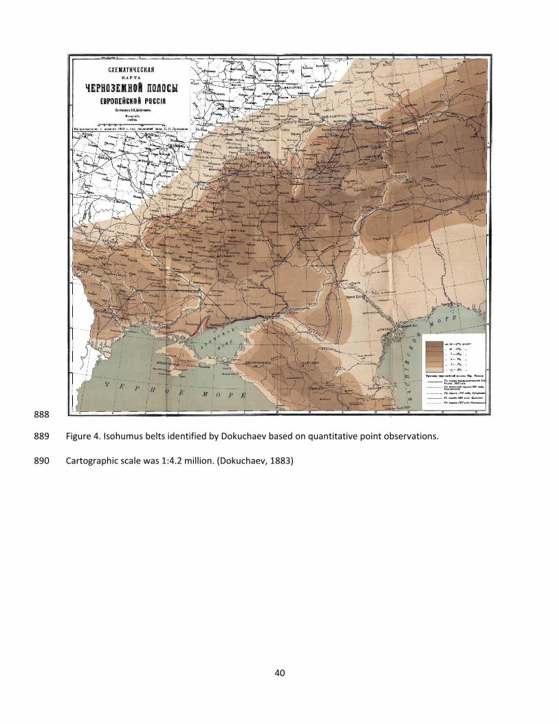
40

888

Figure 4. Isohumus belts identified by Dokuchaev based on quantitative point observations. 889

Cartographic scale was 1:4.2 million. (Dokuchaev, 1883) 890

41

891

Figure 5. Soil map of Africa based on zonal classification system. Cartographic scale was 1:10 million. 892

(Shantz and Marbut, 1923) 893

42

894

Figure 6. General soil map of Wisconsin produced in the agrogeology style by T.C. Chamberlain. 895

Cartographic scale not provided. (Chamberlain, 1882) 896

43

897

Figure 7. Soil map of Tama County, Iowa produced at a cartographic scale of 1:63,360 (Ely et al., 1904). 898

Only five map units are delineated, each of which primarily differ in parent material. Variation of soils 899

due to climate or relief is not included. 900

44

901

Figure 8. Soil regions of Wisconsin map published by the Wisconsin Geological and Natural History 902

Survey. Cartographic scale was 1:710,000 (Madison and Gundlach, 1993). The spatial patterns in this 903

map are very similar to the patterns in the earlier, agrogeology style soil map of Wisconsin. The two 904

maps primarily differ due to more accurate spatial information being available for the modern soil map. 905

45

906

Figure 9. Soil associations of Iowa map published by the Iowa Agriculture and Home Economics Station. 907

Cartographic scale was 1:506,880 (National Cooperative Soil Survey, 1978). This soil map has a level of 908

detail similar to the contemporary soil map of Wisconsin (Figure 7); both primarily represent the spatial 909

distribution of geologic/parent materials. 910

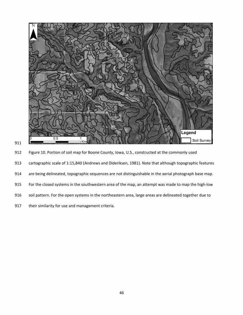
46

911

Figure 10. Portion of soil map for Boone County, Iowa, U.S., constructed at the commonly used 912

cartographic scale of 1:15,840 (Andrews and Dideriksen, 1981). Note that although topographic features 913

are being delineated, topographic sequences are not distinguishable in the aerial photograph base map. 914

For the closed systems in the southwestern area of the map, an attempt was made to map the high-low 915

soil pattern. For the open systems in the northeastern area, large areas are delineated together due to 916

their similarity for use and management criteria. 917

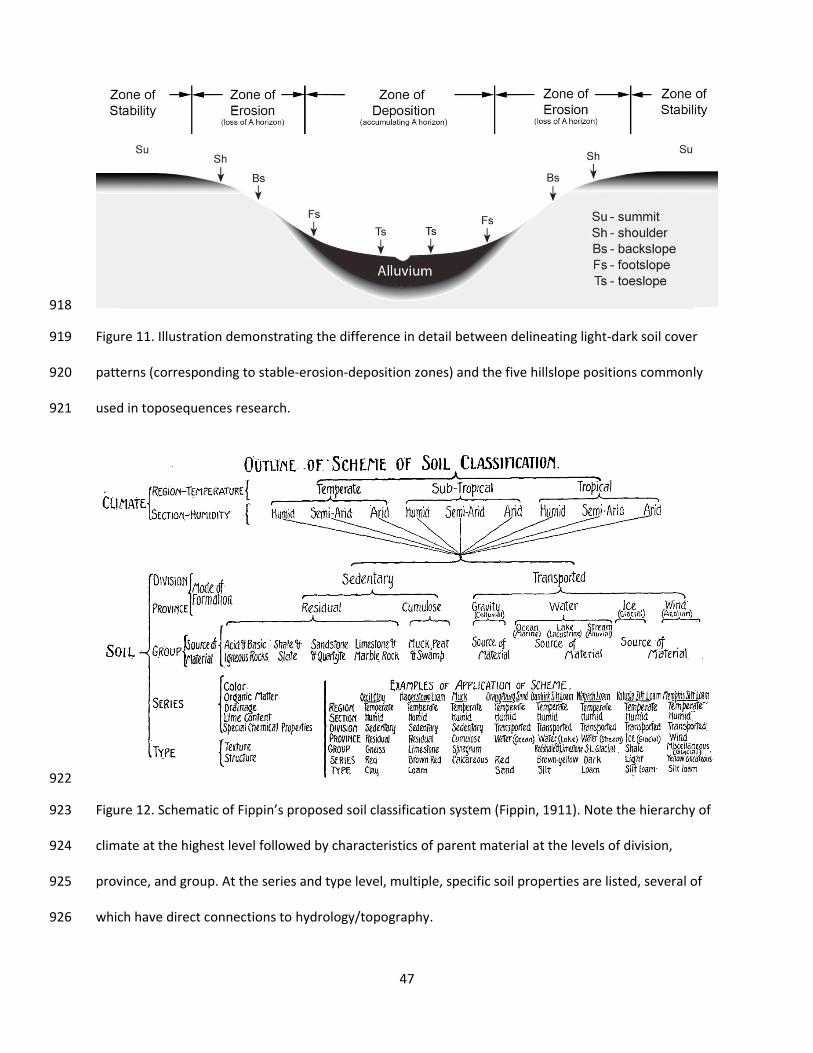
47

918

Figure 11. Illustration demonstrating the difference in detail between delineating light-dark soil cover 919

patterns (corresponding to stable-erosion-deposition zones) and the five hillslope positions commonly 920

used in toposequences research. 921

922

Figure 12. Schematic of Fippin’s proposed soil classification system (Fippin, 1911). Note the hierarchy of 923

climate at the highest level followed by characteristics of parent material at the levels of division, 924

province, and group. At the series and type level, multiple, specific soil properties are listed, several of 925

which have direct connections to hydrology/topography. 926

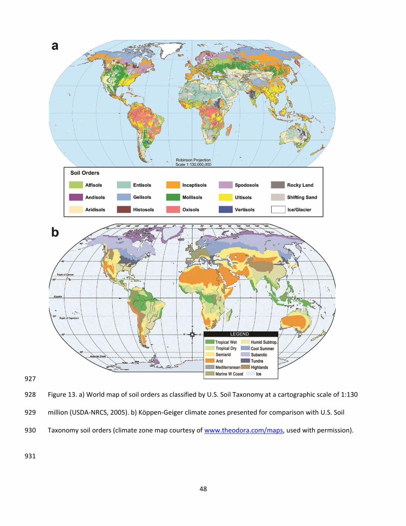
48

927

Figure 13. a) World map of soil orders as classified by U.S. Soil Taxonomy at a cartographic scale of 1:130 928

million (USDA-NRCS, 2005). b) Köppen-Geiger climate zones presented for comparison with U.S. Soil 929

Taxonomy soil orders (climate zone map courtesy of www.theodora.com/maps, used with permission). 930

931

49

Table 1. Relationship between the top levels of zonal classification and the current version of Soil 932 Taxonomy. 933 934

Zonal Intrazonal Azonal

Climate-Vegetation Exceptions based on geology or hydrology Exceptions based on time

Alfisols Histosols Entisols

Aridisols Andisols Inceptisols (some)

Gelisols Vertisols (some)

Mollisols

Oxisols

Spodosols Ultisols Vertisols (some)

Inceptisols (some)

935