RUSSIAN ACADEMY OF SCIENCES Keldysh Institute of Applied Mathematics INSTITUTE OF ORIENTAL STUDIES VOLGOGRAD CENTER FOR SOCIAL RESEARCH HISTORY & MATHEMATICS Trends and Cycles Edited by Leonid E. Grinin, and Andrey V. Korotayev ‘Uchitel’ Publishing House Volgograd

Welcome message from author
This document is posted to help you gain knowledge. Please leave a comment to let me know what you think about it! Share it to your friends and learn new things together.
Transcript

RUSSIAN ACADEMY OF SCIENCES Keldysh Institute of Applied Mathematics
INSTITUTE OF ORIENTAL STUDIES
VOLGOGRAD CENTER FOR SOCIAL RESEARCH
HISTORY & MATHEMATICS
Trends and Cycles
Edited by Leonid E. Grinin,
and Andrey V. Korotayev
‘Uchitel’ Publishing House
Volgograd
ББК 22.318 60.5 ‛History & Mathematics’ Yearbook
Editorial Council: Herbert Barry III (Pittsburgh University), Leonid Borodkin (Moscow State University; Cliometric Society), Robert Carneiro (American Museum of Natural History), Christopher Chase-Dunn (University of California, Riverside), Dmitry Chernavsky (Russian Academy of Sciences), Thessaleno Devezas (University of Beira Interior), Leonid Grinin (National Research Univer-sity Higher School of Economics), Antony Harper (New Trier College), Peter Herrmann (University College of Cork, Ireland), Andrey Korotayev (National Research University Higher School of Economics), Alexander Logunov (Rus-sian State University for the Humanities), Gregory Malinetsky (Russian Acad-emy of Sciences), Sergey Malkov (Russian Academy of Sciences), Charles Spencer (American Museum of Natural History), Rein Taagapera (University of California, Irvine), Arno Tausch (Innsbruck University), William Thompson (University of Indiana), Peter Turchin (University of Connecticut), Douglas White (University of California, Irvine), Yasuhide Yamanouchi (University of Tokyo). History & Mathematics: Trends and Cycles. Yearbook / Edited by Leonid E. Gri- nin and Andrey V. Korotayev. – Volgograd: ‘Uchitel’ Publishing House, 2014. – 328 pp.
The present yearbook (which is the fourth in the series) is subtitled Trends & Cycles. It is devoted to cyclical and trend dynamics in society and nature; special attention is paid to economic and demographic aspects, in particular to the mathematical modeling of the Malthusian and post-Malthusian traps' dynamics.
An increasingly important role is played by new directions in historical research that study long-term dynamic processes and quantitative changes. This kind of history can hardly develop without the application of mathematical methods. There is a tendency to study history as a system of various processes, within which one can detect waves and cycles of different lengths – from a few years to several centuries, or even millennia. The contributions to this yearbook present a qualitative and quantitative analysis of global historical, political, eco-nomic and demographic processes, as well as their mathematical models.
This issue of the yearbook consists of three main sections: (I) Long-Term Trends in Nature and Society; (II) Cyclical Processes in Pre-industrial Societies; (III) Contemporary History and Processes.
We hope that this issue of the yearbook will be interesting and useful both for histo-rians and mathematicians, as well as for all those dealing with various social and natural sciences.
The present research has been carried out in the framework of the project of the National Research University Higher School of Economics.
‛Uchitel’ Publishing House 143 Kirova St., 400079 Volgograd, Russia ISBN 978-5-7057-4223-3 © ‘Uchitel’ Publishing House, 2014 Volgograd 2014
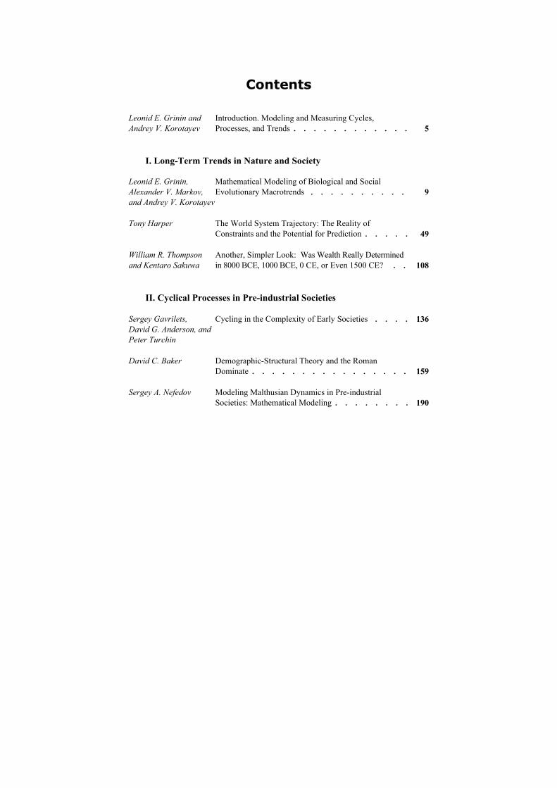
Contents Leonid E. Grinin and Andrey V. Korotayev
Introduction. Modeling and Measuring Cycles, Processes, and Trends . . . . . . . . . . . .
5
I. Long-Term Trends in Nature and Society
Leonid E. Grinin, Alexander V. Markov, and Andrey V. Korotayev
Mathematical Modeling of Biological and Social Evolutionary Macrotrends . . . . . . . . . .
9
Tony Harper The World System Trajectory: The Reality of Constraints and the Potential for Prediction . . . . .
49
William R. Thompson and Kentaro Sakuwa
Another, Simpler Look: Was Wealth Really Determined in 8000 BCE, 1000 BCE, 0 CE, or Even 1500 CE? . .
108
II. Cyclical Processes in Pre-industrial Societies Sergey Gavrilets, David G. Anderson, and Peter Turchin
Cycling in the Complexity of Early Societies . . . .
136
David C. Baker Demographic-Structural Theory and the Roman Dominate . . . . . . . . . . . . . . . .
159
Sergey A. Nefedov Modeling Malthusian Dynamics in Pre-industrial Societies: Mathematical Modeling . . . . . . . .
190
Сontents 4
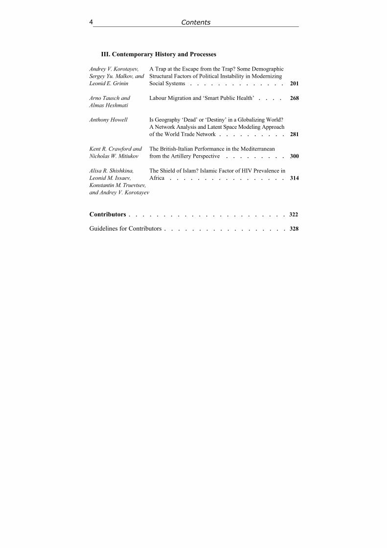
III. Contemporary History and Processes Andrey V. Korotayev, Sergey Yu. Malkov, and Leonid E. Grinin
A Trap at the Escape from the Trap? Some Demographic Structural Factors of Political Instability in Modernizing Social Systems . . . . . . . . . . . . . .
201
Arno Tausch and Almas Heshmati
Labour Migration and ‘Smart Public Health’ . . . .
268
Anthony Howell Is Geography ‘Dead’ or ‘Destiny’ in a Globalizing World? A Network Analysis and Latent Space Modeling Approach of the World Trade Network . . . . . . . . . .
281
Kent R. Crawford and Nicholas W. Mitiukov
The British-Italian Performance in the Mediterranean from the Artillery Perspective . . . . . . . . .
300
Alisa R. Shishkina, Leonid M. Issaev, Konstantin M. Truevtsev, and Andrey V. Korotayev
The Shield of Islam? Islamic Factor of HIV Prevalence in Africa . . . . . . . . . . . . . . . . .
314
Contributors . . . . . . . . . . . . . . . . . . . . . . . 322 Guidelines for Contributors . . . . . . . . . . . . . . . . . . 328
History & Mathematics: Trends and Cycles 2014 5–8
5
Introduction
Modeling and Measuring Cycles,
Processes, and Trends
Leonid E. Grinin and Andrey V. Korotayev The present Yearbook (which is the fourth in the series) is subtitled Trends & Cycles. Already ancient historians (see, e.g., the second Chapter of Book VI of Polybius' Histories) described rather well the cyclical component of historical dynamics, whereas new interesting analyses of such dynamics also appeared in the Medieval and Early Modern periods (see, e.g., Ibn Khaldūn 1958 [1377], or Machiavelli 1996 [1531] 1). This is not surprising as the cyclical dynamics was dominant in the agrarian social systems. With modernization, the trend dynam-ics became much more pronounced and these are trends to which the students of modern societies pay more attention. Note that the term trend – as regards its contents and application – is tightly connected with a formal mathematical analysis. Trends may be described by various equations – linear, exponential, power-law, etc. On the other hand, the cliodynamic research has demonstrated that the cyclical historical dynamics can be also modeled mathematically in a rather effective way (see, e.g., Usher 1989; Chu and Lee 1994; Turchin 2003, 2005a, 2005b; Turchin and Korotayev 2006; Turchin and Nefedov 2009; Nefe-dov 2004; Korotayev and Komarova 2004; Korotayev, Malkov, and Khal-tourina 2006; Korotayev and Khaltourina 2006; Korotayev 2007; Grinin 2007), whereas the trend and cycle components of historical dynamics turn out to be of equal importance.
It is obvious that the qualitative innovative motion toward new, unknown forms, levels, and volumes, etc. cannot continue endlessly, linearly and smoothly. It always has limitations, accompanied by the emergence of imbalances, increas-ing resistance to environmental constraints, competition for resources, etc. These endless attempts to overcome the resistance of the environment created conditions for a more or less noticeable advance in societies. However, relatively short peri-ods of rapid growth (which could be expressed as a linear, exponential or hyper-bolic trend) tended to be followed by stagnation, different types of crises and set-backs, which created complex patterns of historical dynamics, within which trend and cyclical components were usually interwoven in rather intricate ways (see, e.g., Grinin and Korotayev 2009; Grinin, Korotayev, and Malkov 2010).
1 For interpretations of their theories (in terms of cliodynamics, cyclical dynamics etc.) see, e.g.,
Turchin 2003; Korotayev and Khaltourina 2006; Grinin 2012a.
Introduction. Cycles, Processes, and Trends 6
Hence, in history we had a constant interaction of cyclical and trend dy-namics, including some very long-term trends that are analyzed in Section I of the present Yearbook which includes contributions by Leonid E. Grinin, Alexander V. Markov, and Andrey V. Korotayev (‘Mathematical Modeling of Biological and Social Evolutionary Macrotrends’), Tony Harper (‘The World System Trajectory: The Reality of Constraints and the Potential for Prediction’) and William R. Thompson and Kentaro Sakuwa (‘Another, Simpler Look: Was Wealth Really Determined in 8000 BCE, 1000 BCE, 0 CE, or Even 1500 CE?’).
If in a number of societies and for quite a long time we observe regular repetition of a cycle of the same type ending with grave crises and significant setbacks, this means that at a given level of development we confront such rigid and strong systemic and environmental constraints which the given soci-ety is unable to overcome.
Thus, the notion of cycle is closely related to the concept of the trap. In the language of nonlinear dynamics the concept of traps will more or less corre-spond to the term ‘attractor’. Continuing the comparison with nonlinear dy-namics, we should say that a steady escape from the trap will largely corre-spond to the concept of a phase transition.
In this Yearbook particular attention is paid, of course, to the Malthusian trap. The escape from the Malthusian trap in historical retrospect was incredi-bly difficult (see, e.g., Korotayev et al. 2011; Grinin 2012b). Periodically, at-tempts were made to get out of this trap. However, for many millennia no so-cieties managed to achieve a final steady escape from it, but those attempts in the long run led to a systematic increase in the level of technological develop-ment of the World System.
The problems of the mathematical modeling of the Malthusian trap dynam-ics are analyzed in the article by Sergey A. Nefedov (‘Modeling Malthusian Dynamics in Pre-Industrial Societies: Mathematical Modeling’) in Section II of the present issue of the Yearbook. This section also includes the article by Ser-gey Gavrilets, David G. Anderson, and Peter Turchin (‘Cycling in the Com-plexity of Early Societies’), as well as the one by David C. Baker (‘Demo-graphic-Structural Theory and the Roman Dominate’). These articles deal with various cycles in the historical dynamics of pre-Modern social systems that are rather tightly connected with demographic macroprocesses. The first arti-cle of the next section also deals with the problems of the escape from the Malthusian trap.
Section III deals with Modern history and contemporary processes and in-cludes the contribution by Andrey V. Korotayev, Sergey Yu. Malkov, and Leonid E. Grinin (‘A Trap at the Escape from the Trap? Some Demographic Structural Factors of Political Instability in Modernizing Social Systems’) con-tinuing the discussion on the issues of the Malthusian and post-Malthusian traps. This issue is also touched upon in the contributions by Arno Tausch
Leonid E. Grinin and Andrey V. Korotayev 7
and Almas Heshmati (‘Labour Migration and “Smart Public Health”’), An-thony Howell (‘Is Geography “Dead” or “Destiny” in a Globalizing World? A Network Analysis and Latent Space Modeling Approach of the World Trade Network’), Kent R. Crawford and Nicholas W. Mitiukov (‘The British-Italian Performance in the Mediterranean from the Artillery Perspective’), as well as Alisa R. Shishkina, Leonid M. Issaev, Konstan- tin M. Truevtsev, and Andrey V. Korotayev (‘The Shield of Islam? Islamic Factor of HIV Prevalence in Africa’).
Articles in this section are devoted to some rather interesting aspects and events from the Second World War to the prospects for change of the age com-position of the Earth's population in the coming decades. What appears valu-able is that the contributors have managed to somehow formalize these proc-esses, and to apply various mathematical techniques to the analysis of the re-cent historical processes.
References
Chu C. Y. C., and Lee R. D. 1994. Famine, Revolt, and the Dynastic Cycle: Population Dynamics in Historic China. Journal of Population Economics 7: 351–378.
Grinin L. E. 2007. The Correlation between the Size of Society and Evolutionary Type of Polity. History and Mathematics: The Analysis and Modeling of Socio-historical Proc-esses / Ed. by A. V. Korotayev, S. Yu. Malkov, and L. E. Grinin, pp. 263–303. Mos-cow: KomKniga/URSS. In Russian (Гринин Л. Е. Зависимость между размерами общества и эволюционным типом политии. История и математика: анализ и моделирование социально-исторических процессов / ред. А. В. Коротаев, С. Ю. Малков, Л. Е. Гринин, с. 263–303. М.: КомКнига).
Grinin L. E. 2012a. From Confucius to Comte. Formation of the Theory, Methodology and Philosophy of History / ed. by A. V. Korotayev. Moscow: LIBROKOM. In Rus-sian (Гринин. Л. Е. От Конфуция до Конта. Становление теории, методологии и философии истории / отв. ред. А. В. Коротаев. М.: ЛИБРОКОМ).
Grinin L. E. 2012b. State and Socio-Political Crises in the Process of Modernization. Cliodynamics 3: 124–157.
Grinin L. E., and Korotayev A. V. 2009. Social Macroevolution: Growth of the World System Integrity and a System of Phase Transitions. World Futures 65(7): 477–506.
Grinin L., Korotayev A., and Malkov S. 2010. A Mathematical Model of Juglar Cy-cles and the Current Global Crisis. History & Mathematics. Processes and Models of Global Dynamics / Ed. by L. Grinin, P. Herrmann, A. Korotayev, and A. Tausch, pp. 138–187. Volgograd: Uchitel.
Ibn Khaldūn `Abd al-Rahman. 1958 [1377]. The Muqaddimah: An Introduction to His-tory. New York, NY: Pantheon Books (Bollingen Series, 43).
Korotayev A. 2007. Secular Cycles and Millennial Trends: A Mathematical Model. Mathematical Modeling of Social and Economic Dynamics / Ed. by M. G. Dmitriev, A. P. Petrov, and N. P. Tretyakov, pp. 118–125. Moscow: RUDN.
Introduction. Cycles, Processes, and Trends 8
Korotayev A., and Khaltourina D. 2006. Introduction to Social Macrodynamics: Secu-lar Cycles and Millennial Trends in Africa. Moscow: KomKniga/URSS.
Korotayev A., and Komarova N. 2004. A New Mathematical Model of Pre-Industrial Demographic Cycle. Mathematical Modeling of Social and Economic Dynamics / Ed. by M. G. Dmitriev, and A. P. Petrov, pp. 157–163. Moscow: Russian State Social University.
Korotayev A., Malkov A., and Khaltourina D. 2006. Introduction to Social Macrody-namics: Secular Cycles and Millennial Trends. Moscow: KomKniga/URSS.
Korotayev A., Zinkina J., Kobzeva S., Bogevolnov J., Khaltourina D., Malkov A., and Malkov S. 2011. A Trap at the Escape from the Trap? Demographic-Structural Factors of Political Instability in Modern Africa and West Asia. Cliodynamics: The Journal of Theoretical and Mathematical History 2(2): 276–303.
Machiavelli N. 1996 [1531]. Discourses on Livy. Chicago, IL: University of Chicago Press.
Nefedov S. A. 2004. A Model of Demographic Cycles in Traditional Societies: The Case of Ancient China. Social Evolution & History 3(1): 69–80.
Turchin P. 2003. Historical Dynamics: Why States Rise and Fall. Princeton, NJ: Princeton University Press.
Turchin P. 2005a. Dynamical Feedbacks between Population Growth and Sociopoliti-cal Instability in Agrarian States. Structure and Dynamics 1: 1–19.
Turchin P. 2005b. War and Peace and War: Life Cycles of Imperial Nations. New York: Pi Press.
Turchin P., and Korotayev А. 2006. Population Density and Warfare: A Reconsidera-tion. Social Evolution & History 5(2): 121–158.
Turchin P., and Nefedov S. 2009. Secular Cycles. Princeton, NJ: Princeton University Press.
Usher D. 1989. The Dynastic Cycle and the Stationary State. The American Economic Review 79: 1031–1044.
History & Mathematics: Trends and Cycles 2014 9–48
9
I. LONG-TERM TRENDS IN NATURE AND SOCIETY
1
Mathematical Modeling of Biological and Social Evolutionary Macrotrends*
Leonid E. Grinin, Alexander V. Markov,
and Andrey V. Korotayev
Abstract
In the first part of this article we survey general similarities and differences between biological and social macroevolution. In the second (and main) part, we consider a concrete mathematical model capable of describing important features of both biological and social macroevolution. In mathematical models of historical macrodynamics, a hyperbolic pattern of world population growth arises from non-linear, second-order positive feedback between demographic growth and technological development. Based on diverse paleontological data and an analogy with macrosociological models, we suggest that the hyperbolic character of biodiversity growth can be similarly accounted for by non-linear, second-order positive feedback between diversity growth and the complexity of community structure. We discuss how such positive feedback mechanisms can be modelled mathematically.
Keywords: social evolution, biological evolution, mathematical model, bio-diversity, population growth, positive feedback, hyperbolic growth.
Introduction
The present article represents an attempt to move further in our research on the similarities and differences between social and biological evolution (see Grinin, Markov et al. 2008, 2009a, 2009b, 2011, 2012). We have endeavored to make a systematic comparison between biological and social evolution at different levels of analysis and in various aspects. We have formulated a considerable number of general principles and rules of evolution, and worked to develop a common terminology to describe some key processes in biological and social evolution. In particular, we have introduced the notion of ‘social aromorphosis’
* This research has been supported by the Russian Science Foundation (Project No 14-11-00634).
Modeling of Biological and Social Macrotrends 10
to describe the process of widely diffused social innovation that enhances the complexity, adaptability, integrity, and interconnectedness of a society or social system (Grinin, Markov et al. 2008, 2009a, 2009b). This work has convinced us that it might be possible to find mathematical models that can describe im-portant features of both biological and social macroevolution. In the first part of this article we survey general similarities and differences between the two types of macroevolution. In the second (and main) part, we consider a concrete math-ematical model that we deem capable of describing important features of both biological and social macroevolution.
The comparison of biological and social evolution is an important but (un-fortunately) understudied subject. Students of culture still vigorously debate the applicability of Darwinian evolutionary theory to social/cultural evolution. Un-fortunately, the result is largely a polarization of views. On the one hand, there is a total rejection of Darwin's theory of social evolution (see, e.g., Hallpike 1986). On the other hand, there are arguments that cultural evolution demon-strates all of the key characteristics of Darwinian evolution (Mesoudi et al. 2006).
We believe that, instead of following the outdated objectivist principle of ‘either – or’, we should concentrate on the search for methods that could allow us to apply the achievements of evolutionary biology to understanding social evolution and vice versa. In other words, we should search for productive gen-eralizations and analogies for the analysis of evolutionary mechanisms in both contexts. The Universal Evolution approach aims for the inclusion of all mega-evolution within a single paradigm (discussed in Grinin, Carneiro, et al. 2011). Thus, this approach provides an effective means by which to address the above-mentioned task.
It is not only systems that evolve, but also mechanisms of evolution (see Grinin, Markov, and Korotayev 2008). Each sequential phase of macroevolu-tion is accompanied by the emergence of new evolutionary mechanisms. Cer-tain prerequisites and preadaptations can, therefore, be detected within the pre-vious phase, and the development of new mechanisms does not invalidate the evolutionary mechanisms that were active during earlier phases. As a result, one can observe the emergence of a complex system of interaction composed of the forces and mechanisms that work together to shape the evolution of new forms.
Biological organisms operate in the framework of certain physical, chemi-cal and geological laws. Likewise, the behaviors of social systems and people have certain biological limitations (naturally, in addition to various social-structural, historical, and infrastructural limitations). From the standpoint of Universal Evolution, new forms of evolution that determine phase transitions may result from activities going in different directions. Some forms that are similar in principle may emerge at breakthrough points, but may also result in evolutionary dead-ends. For example, social forms of life emerged among
Leonid E. Grinin, Alexander V. Markov, and Andrey V. Korotayev 11
many biological phyla and classes, including bacteria, insects, birds, and mammals. Among insects, in particular, one finds rather highly developed forms of socialization (see, e.g., Robson and Traniello 2002; Ryabko and Rez-nikova 2009; Reznikova 2011). Yet, despite the seemingly common trajectory and interrelation of social behaviors among these various life forms, the im-pacts that each have had on the Earth are remarkably different.
Further, regarding information transmission mechanisms, it appears possi-ble to speak about certain ‘evolutionary freaks’. Some of these mechanisms were relatively widespread in the biological evolution of simple organisms, but later became less so. Consider, for example, the horizontal exchange of genetic information (genes) among microorganisms, which makes many useful genetic ‘inventions’ available in a sort of ‘commons’ for microbe communities. Among bacteria, the horizontal transmission of genes contributes to the rapid develop-ment of antibiotic resistance (e.g., Markov and Naymark 2009). By contrast, this mechanism of information transmission became obsolete or was trans-formed into highly specialized mechanisms (e.g., sexual reproduction) in the evolution of more complex organisms. Today, horizontal transmission is mostly confined to the simplest forms of life.
These examples suggest that an analysis of the similarities and differences between the mechanisms of biological and social evolution may help us to un-derstand the general principles of megaevolution1 in a much fuller way. These similarities and differences may also reveal the driving forces and supra-phase mechanisms (i.e., mechanisms that operate in two or more phases) of megaevo-lution. One of our previous articles was devoted to the analysis of one such mechanism: aromorphosis, the process of widely diffused social innovation that enhances the complexity, adaptability, integrity, and interconnectedness of a so-ciety or social system (Grinin, Markov, and Korotayev 2011; see also Grinin and Korotayev 2008, 2009a, 2009b; Grinin, Markov, and Korotayev 2009a, 2009b).
It is important to carefully compare the two types of macroevolution (i.e., biological and social) at various levels and in various aspects. This is necessary because such comparisons often tend to be incomplete and deformed by con-ceptual extremes. These limitations are evident, for example, in the above-referenced paper by Mesoudi et al. (2006), which attempts to apply a Darwin-ian method to the study of social evolution. Unfortunately, a failure to recog-nize or accept important differences between biological and social evolution reduces the overall value of the method that these authors propose. Christopher Hallpike's rather thorough monograph, Principles of Social Evolution (1986), provides another illustration of these limitations. Here, Hallpike offers a fairly complete analysis of the similarities and differences between social and bio- 1 We denote as megaevolution all the process of evolution throughout the whole of Big History,
whereas we denote as macroevolution the process of evolution during one of its particular phases.
Modeling of Biological and Social Macrotrends 12
logical organisms, but does not provide a clear and systematic comparison be-tween social and biological evolution. In what follows, we hope to avoid simi-lar pitfalls.
Biological and Social Evolution: A Comparison at Various Levels
There are a few important differences between biological and social macroevo-lution. Nonetheless, it is possible to identify a number of fundamental similari-ties, including at least three basic sets of shared factors. First, we are discussing very complex, non-equilibrium, but stable systems whose function and evolu-tion can be described by General Systems Theory, as well as by a number of cybernetic principles and laws. Second, we are not dealing with isolated sys-tems, but with the complex interactions between organisms and their external environments. As a result, the reactions of systems to ‘external’ challenges can be described in terms of general principles that express themselves within a biological reality and a social reality. Third (and finally), a direct ‘genetic’ link exists between the two types of macroevolution and their mutual influence.
We believe that the laws and forces driving the biological and social phas-es of Big History can be comprehended more effectively if we apply the con-cept of biological and social aromorphosis (Grinin, Markov, and Korotayev 2011). There are some important similarities between the evolutionary algo-rithms of biological and social aromorphoses. Thus, it has been noticed that the basis of biological aromorphosis
is usually formed by some partial evolutionary change that... creates sig-nificant advantages for an organism, puts it in more favorable conditions for reproduction, multiplies its numbers and its changeability..., thus ac-celerating the speed of its further evolution. In those favorable condi-tions, the total restructurization of the whole organization takes place af-terwards (Shmal'gauzen 1969: 410; see also Severtsov 1987: 64–76).
During the course of adaptive radiation, such changes in organization dif-fuse more or less widely (frequently with significant variations).
A similar pattern is observed within social macroevolution. An example is the invention and diffusion of iron metallurgy. Iron production was practiced sporadically in the 3rd millennium BCE, but regular production of low-grade steel did not begin until the mid-2nd millennium BCE in Asia Minor (see, e.g., Chubarov 1991: 109). At this point, the Hittite kingdom guarded its monopoly over the new technology. The diffusion of iron technology led to revolutionary changes in different spheres of life, including a significant advancement in plough agriculture and, consequently, in the agrarian system as a whole (Grinin and Korotayev 2006); an intensive development of crafts; an increase in urban-
Leonid E. Grinin, Alexander V. Markov, and Andrey V. Korotayev 13
ism; the formation of new types of militaries, armed with relatively cheap but effective iron weapons; and the emergence of significantly more developed systems of taxation, as well as information collection and processing systems, that were necessary to support these armies (e.g., Grinin and Korotayev 2007a, 2007b). Ironically, by introducing cheaply made weapons and other tools into the hands of people who might resist the Hittite state, this aromorphosis not only supported the growth of that kingdom, it also laid the groundwork for his-torical phase shifts.
Considering such cases through the lens of aromorphosis has helped us to detect a number of regularities and rules that appear to be common to biological and social evolution (Grinin, Markov, and Korotayev 2011). Such rules and regularities (e.g., payment for arogenic progress, special conditions for the emergence of aromorphosis, etc.) are similar for both biological and social macroevolution. It is important to emphasize, however, that similarity between the two types of macroevolution does not imply commonality. Rather, signifi-cant similarities are frequently accompanied by enormous differences. For ex-ample, the genomes of chimpanzees and the humans are 98 per cent similar, yet there are enormous intellectual and social differences between chimpanzees and humans that arise from the apparently ‘insignificant’ variations between the two genomes (see Markov and Naymark 2009).
Despite its aforementioned limitations, it appears reasonable to continue the comparison between the two types of macroevolution following the analysis offered by Hallpike (1986). Therefore, it may prove useful to revisit the perti-nent observations of this analysis here. Table 1 summarizes the similarities and differences that Hallpike (1986: 33–34) finds between social and biological organisms.
While we do not entirely agree with all of his observations – for example, the establishment of colonies could be seen as a kind of social reproduction akin to organic reproduction – we do feel that Hallpike comes to a sound con-clusion: that similarities between social and biological organisms are, in gen-eral, determined by similarities in organization and structure (we would say similarities between different types of systems). As a result, Hallpike believes that one can use certain analogies in which institutions are similar to some or-gans. In this way, cells may be regarded as similar to individuals, central gov-ernment similar to the brain, and so on. Examples of this kind of thinking can be found in the classic texts of social theory (see, e.g., Spencer 1898 and Durk-heim 1991 [1893]), as well as in more recent work (see, e.g., Heylighen 2011).

Modeling of Biological and Social Macrotrends 14
Table 1. Similarities and differences between social and biological organisms, as described by Hallpike (1986)
Similarities Differences
Social institutions are interrelated in a man-ner analogous to the organs of the body.
Individual societies do not have clear boundaries. For example, two societies may be distinct politically, but not cul-turally or religiously.
Despite changes in membership, social institutions maintain continuity, as do biological organs when individual cells are replaced.
Unlike organic cells, the individuals within a society have agency and are capable of learning from experience.
The social division of labor is analogous to the specialization of organic functions.
Social structure and function are far less closely related than in organic structure and function.
Self-maintenance and feedback processes characterize both kinds of system.
Societies do not reproduce. Cultural transmission between generations can-not be distinguished from the processes of system maintenance.
Adaptive responses to the physical envi-ronment characterize both kinds of sys-tem.
Societies are more mutable than organ-isms, displaying a capacity for meta-morphosis only seen in organic phylog-eny.
The trade, communication, and other transmission processes that characterize social systems are analogous to the proc-esses that transmit matter, energy, and information in biological organisms.
Societies are not physical entities, rather their individual members are linked by information bonds.
When comparing biological species and societies, Hallpike (1986: 34) sin-gles out the following similarities:
(1) that, like societies, species do not reproduce, (2) that both have phylogenies reflecting change over time, and (3) that both are made up of individuals who compete against one another. Importantly, he also indicates the following difference: ‘[S]ocieties are or-
ganized systems, whereas species are simply collections of individual organ-isms’ (Hallpike 1986: 34).
Hallpike tries to demonstrate that, because of the differences between bio-logical and social organisms, the very idea of natural selection does not appear to apply to social evolution. However, we do not find his proofs very convinc-ing on this account, although they do make sense in certain respects. Further,
Leonid E. Grinin, Alexander V. Markov, and Andrey V. Korotayev 15
his analysis is confined mainly to the level of the individual organism and the individual society. He rarely considers interactions at the supra-organism level (though he does, of course, discuss the evolution of species). His desire to dem-onstrate the sterility of Darwinian theory to discussions of social evolution not-withstanding, it seems that Hallpike involuntarily highlights the similarity be-tween biological and social evolution. As he, himself, admits, the analogy between the biological organism and society is quite noteworthy.
Just as he fails to discuss interactions and developments at the level of the supra-organism in great detail, Hallpike does not take into account the point in social evolution where new supra-societal developments emerge (up to the lev-el of the emergence of the World System [e.g., Korotayev 2005, 2007, 2008, 2012; Grinin and Korotayev 2009b]). We contend that it is very important to consider not only evolution at the level of a society but also at the level above individual societies, as well as the point at which both levels are interconnected. The supra-organism level is very important to understanding biological evolution, though the differences between organisms and societies make the importance of this supra-level to understanding social evolution unclear. Thus, it might be more productive to compare societies with ecosystems rather than with organisms or species. However, this would demand the development of special methods, as it would be necessary to consider the society not as a social organism, but as a part of a wider system, which includes the natural and social environment (cf., Leke-vičius 2009, 2011).
In our own analysis, we seek to build on the observations of Hallpike while, at the same time, providing a bit more nuance and different scales of analysis. Viewing each as a process involving selection (natural, social, or both), we identify the differences between social and biological evolution at the level of the individual biological organism and individual society, as well as at the supra-organismic and supra-societal level.
Natural and Social Selection Biological evolution is more additive (cumulative) than substitutive. Put an-other way: the new is added to the old. By contrast, social evolution (especially over the two recent centuries) is more substitutive than additive: the new re-places the old (Grinin, Markov et al. 2008, 2011).
Further, the mechanisms that control the emergence, fixation, and diffusion of evolutionary breakthroughs (aromorphoses) differ between biological and social evolution. These differences lead to long-term restructuring in the size and complexity of social organisms. Unlike biological evolution, where some growth of complexity is also observed, social reorganization becomes continu-ous. In recent decades, societies that do not experience a constant and signifi-cant evolution look inadequate and risk extinction.
Modeling of Biological and Social Macrotrends 16
In addition, the size of societies (and systems of societies) tends to grow constantly through more and more tightly integrative links (this trend has be-come especially salient in recent millennia), whereas the trend towards increase in the size of biological organisms in nature is rather limited and far from gen-eral. At another level of analysis, one can observe the formation of special su-prasocietal systems that also tend to grow in size. This is one of the results of social evolution and serves as a method of aromorphosis fixation and diffusion.
The Individual Biological Organism and the Individual Society It is very important to note that, although biological and social organisms are significantly (actually ‘systemically’) similar, they are radically different in their capacities to evolve. For example, as indicated by Hallpike (see above), societies are capable of rapid evolutionary metamorphoses that were not ob-served in the pre-human organic world. In biological evolution, the characteris-tics acquired by an individual are not inherited by its offspring; thus, they do not influence the very slow process of change.
There are critical differences in how biological and social information are transmitted during the process of evolution. Social systems are not only capable of rapid transformation, they are also able to borrow innovations and new ele-ments from other societies. Social systems may also be transformed con-sciously and with a certain purpose. Such characteristics are absent in natural biological evolution.
The biological organism does not evolve by itself: evolution may only take place at a higher level (e.g., population, species, etc.). By contrast, social evolu-tion can often be traced at the level of the individual social organism (i.e., soci-ety). Moreover, it is frequently possible to trace the evolution of particular in-stitutions and subsystems within a social organism. In the process of social evo-lution the same social organism or institution may experience radical transfor-mation more than once.
The Supra-organic and Supra-societal Level Given the above-mentioned differences, within the process of social evolution we observe the formation of two types of special supra-societal entity: (1) amalgamations of societies with varieties of complexity that have analogues in biological evolution, and (2) elements and systems that do not belong to any particular society and lack many analogues in biological evolution.
The first type of amalgamation is rather typical, not only in social but also in biological evolution. There is, however, a major difference between the two kinds of evolution. Any large society usually consists of a whole hierarchy of social systems. For example, a typical agrarian empire might include nuclear families, extended families, clan communities, village communities, primary districts, secondary districts, and provinces, each operating with their own rules
Leonid E. Grinin, Alexander V. Markov, and Andrey V. Korotayev 17
of interaction but at the same time interconnected. This kind of supra-societal amalgamation can hardly be compared with a single biological organism (though both systems can still be compared functionally, as is correctly noted by Hallpike [1986]). Within biological evolution, amalgamations of organisms with more than one level of organization (as found in a pack or herd) are usu-ally very unstable and are especially unstable among highly organized animals. Of course, analogues do exist within the communities of some social animals (e.g., social insects, primates). Neither should we forget that scale is important: while we might compare a society with an individual biological organism, we must also consider groups of organisms bound by cooperative relationships (see, e.g., Boyd and Richerson 1996; Reeve and Hölldobler 2007). Such groups are quite common among bacteria and even among viruses. These caveats aside, it remains the case that within social evolution, one observes the emer-gence of more and more levels: from groups of small sociums to humankind as a whole.
The multiplication of these levels rapidly produces the second kind of amalgamation. It is clear that the level of analysis is very important for com-parison of biological and social evolution. Which systems should be compared? Analogues appear to be more frequent when a society (a social organism) is compared to a biological organism or species. However, in many cases, it may turn out to be more productive to compare societies with other levels of the biota's systemic organization. This might entail comparisons with populations, ecosystems and communities; with particular structural elements or blocks of communities (e.g., with particular fragments of trophic networks or with par-ticular symbiotic complexes); with colonies; or with groups of highly organized animals (e.g., cetaceans, primates, and other social mammals or termites, ants, bees and other social insects).
Thus, here we confront a rather complex and rarely studied methodological problem: which levels of biological and social process are most congruent? What are the levels whose comparison could produce the most interesting re-sults? In general, it seems clear that such an approach should not be a mechani-cal equation of ‘social organism = biological organism’ at all times and in every situation. The comparisons should be operational and instrumental. This means that we should choose the scale and level of social and biological phenomena, forms, and processes that are adequate for and appropriate to our intended comparisons.
Again, it is sometimes more appropriate to compare a society with an indi-vidual biological organism, whereas in other cases it could well be more appro-priate to compare the society with a community, a colony, a population, or a species. At yet another scale, as we will see below, in some cases it appears rather fruitful to compare the evolution of the biosphere with the evolution of the anthroposphere.
Modeling of Biological and Social Macrotrends 18
Mathematical Modeling of Biological and Social Macroevolution
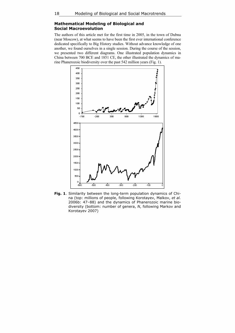
The authors of this article met for the first time in 2005, in the town of Dubna (near Moscow), at what seems to have been the first ever international conference dedicated specifically to Big History studies. Without advance knowledge of one another, we found ourselves in a single session. During the course of the session, we presented two different diagrams. One illustrated population dynamics in China between 700 BCE and 1851 CE, the other illustrated the dynamics of ma-rine Phanerozoic biodiversity over the past 542 million years (Fig. 1).
Fig. 1. Similarity between the long-term population dynamics of Chi-na (top: millions of people, following Korotayev, Malkov, et al. 2006b: 47–88) and the dynamics of Phanerozoic marine bio-diversity (bottom: number of genera, N, following Markov and Korotayev 2007)
Leonid E. Grinin, Alexander V. Markov, and Andrey V. Korotayev 19
The similarity between the two diagrams was striking. This, despite the fact that they depicted the development of very different systems (human popula-tion vs. biota) at different time scales (hundreds of years vs. millions of years), and had been generated using the methods of different sciences (historical de-mography vs. paleontology) with different sources (demographic estimates vs. paleontological data). What could have caused similarity of developmental dy-namics in very different systems?
* * * In 1960, von Foerster et al. published a striking discovery in the journal
Science. They showed that between 1 and 1958 CE, the world's population (N) dynamics could be described in an extremely accurate way with an astonish-ingly simple equation:2
)( 0 tt
CN t
, (Eq. 1)
where Nt is the world population at time t, and C and t0 are constants, with t0 corresponding to an absolute limit (‘singularity’ point) at which N would be-come infinite. Parameter t0 was estimated by von Foerster and his colleagues as 2026.87, which corresponds to November 13, 2026; this made it possible for them to supply their article with a title that was a public-relations masterpiece: ‘Doomsday: Friday, 13 November, A.D. 2026’.
Of course, von Foerster and his colleagues did not imply that the world population on that day could actually become infinite. The real implication was that the world population growth pattern that operated for many centuries prior to 1960 was about to end and be transformed into a radically different pattern. This prediction began to be fulfilled only a few years after the ‘Doomsday’ paper was published as World System growth (and world population growth in particular) began to diverge more and more from the previous blow-up regime. Now no longer hyperbolic, the world population growth pattern is closer to a logistic one (see, e.g., Korotayev, Malkov et al. 2006a; Korotayev 2009).
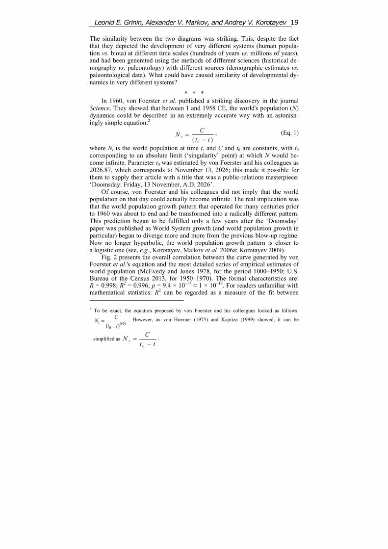
Fig. 2 presents the overall correlation between the curve generated by von Foerster et al.'s equation and the most detailed series of empirical estimates of world population (McEvedy and Jones 1978, for the period 1000–1950; U.S. Bureau of the Census 2013, for 1950–1970). The formal characteristics are: R = 0.998; R2 = 0.996; p = 9.4 × 10⁻¹⁷ ≈ 1 × 10–16. For readers unfamiliar with mathematical statistics: R2 can be regarded as a measure of the fit between 2 To be exact, the equation proposed by von Foerster and his colleagues looked as follows:
99.00 )( tt
CNt
. However, as von Hoerner (1975) and Kapitza (1999) showed, it can be
simplified as tt
CN t
0
.
Modeling of Biological and Social Macrotrends 20
the dynamics generated by a mathematical model and the empirically observed situation, and can be interpreted as the proportion of the variation accounted for by the respective equation. Note that 0.996 also can be expressed as 99.6 %.3 Thus, von Foerster et al.'s equation accounts for an astonishing 99.6 % of all the macrovariation in world population, from 1000 CE through 1970, as esti-mated by McEvedy and Jones (1978) and the U.S. Bureau of the Census (2013).4 Note also that the empirical estimates of world population find them-selves aligned in an extremely neat way along the hyperbolic curve, which con-vincingly justifies the designation of the pre-1970s world population growth pattern as ‘hyperbolic’.
Fig. 2. Correlation between empirical estimates of world population
(black, in millions of people, 1000–1970) and the curve gen-erated by von Foerster et al.'s equation (grey)
3 The second characteristic (p, standing for ‘probability’) is a measure of the correlation's statistical
significance. A bit counter-intuitively, the lower the value of p, the higher the statistical signifi-cance of the respective correlation. This is because p indicates the probability that the observed correlation could be accounted solely by chance. Thus, p = 0.99 indicates an extremely low statis-tical significance, as it means that there are 99 chances out of 100 that the observed correlation is the result of a coincidence, and, thus, we can be quite confident that there is no systematic rela-tionship (at least, of the kind that we study) between the two respective variables. On the other hand, p = 1 × 10–16 indicates an extremely high statistical significance for the correlation, as it means that there is only one chance out of 10,000,000,000,000,000 that the observed correlation is the result of pure coincidence (a correlation is usually considered statistically significant once p < 0.05).
4 In fact, with slightly different parameters (С = 164890.45; t0 = 2014) the fit (R2) between the dynamics generated by von Foerster's equation and the macrovariation of world population for 1000–1970 CE as estimated by McEvedy and Jones (1978) and the U.S. Bureau of the Census (2013) reaches 0.9992 (99.92 %); for 500 BCE – 1970 CE this fit increases to 0.9993 (99.93 %) with the following parameters: С = 171042.78; t0 = 2016.
Leonid E. Grinin, Alexander V. Markov, and Andrey V. Korotayev 21
The von Foerster et al.'s equation, tt
CN t
0
, is the solution for the fol-
lowing differential equation (see, e.g., Korotayev, Malkov et al. 2006a: 119–120):
C
N
dt
dN 2
. (Eq. 2)
This equation can be also written as:
2aNdt
dN ,
(Eq. 3)
where C
a1
.
What is the meaning of this mathematical expression? In our context, dN/dt denotes the absolute population growth rate at a certain moment in time. Hence, this equation states that the absolute population growth rate at any moment in time should be proportional to the square of world population at this moment. This significantly demystifies the problem of hyperbolic growth. To explain this hyperbolic growth, one need only explain why for many millennia the world population's absolute growth rate tended to be proportional to the square of the population.
The main mathematical models of hyperbolic growth in the world popula-tion (Taagapera 1976, 1979; Kremer 1993; Cohen 1995; Podlazov 2004; Tsirel 2004; Korotayev 2005, 2007, 2008, 2009, 2012; Korotayev, Malkov et al. 2006a: 21–36; Golosovsky 2010; Korotayev and Malkov 2012) are based on the following two assumptions:
(1) ‘the Malthusian (Malthus 1978 [1798]) assumption that population is limited by the available technology, so that the growth rate of population is proportional to the growth rate of technology’ (Kremer 1993: 681–682),5 and (2) the idea that ‘[h]igh population spurs technological change because it increases the number of potential inventors… In a larger population there will be proportionally more people lucky or smart enough to come up with new ideas’, thus, ‘the growth rate of technology is proportional to total population’(Kremer 1993: 685).6
Here Kremer uses the main assumption of Endogenous Technological Growth theory (see, e.g., Kuznets 1960; Grossman and Helpman 1991; Aghion
5 In addition to this, the absolute growth rate is proportional to the population itself. With a given
relative growth rate, a larger population will increase more in absolute number than a smaller one. 6 Note that ‘the growth rate of technology’ here means the relative growth rate (i.e., the level to
which technology will grow in a given unit of time in proportion to the level observed at the be-ginning of this period).
Modeling of Biological and Social Macrotrends 22
and Howitt 1998; Simon 1977, 2000; Komlos and Nefedov 2002; Jones 1995, 2005).
The first assumption looks quite convincing. Indeed, throughout most of human history the world population was limited by the technologically deter-mined ceiling of the carrying capacity of land. For example, with foraging sub-sistence technologies the Earth could not support more than 8 million people because the amount of naturally available useful biomass on this planet is lim-ited. The world population could only grow over this limit when people started to apply various means to artificially increase the amount of available biomass that is with the transition from foraging to food production. Extensive agricul-ture is also limited in terms of the number of people that it can support. Thus, further growth of the world population only became possible with the intensifi-cation of agriculture and other technological improvements (see, e.g., Turchin 2003; Korotayev, Malkov et al. 2006a, 2006b; Korotayev and Khaltourina 2006). However, as is well known, the technological level is not constant, but variable (see, e.g., Grinin 2007a, 2007b, 2012), and in order to describe its dy-namics the second basic assumption is employed.
As this second supposition was, to our knowledge, first proposed by Simon Kuznets (1960), we shall denote the corresponding type of dynamics as ‘Kuz-netsian’. (The systems in which the Kuznetsian population-technological dy-namics are combined with Malthusian demographic dynamics will be denoted as ‘Malthusian-Kuznetsian’.) In general, we find this assumption rather plausi-ble – in fact, it is quite probable that, other things being equal, within a given period of time, five million people will make approximately five times more inventions than one million people.
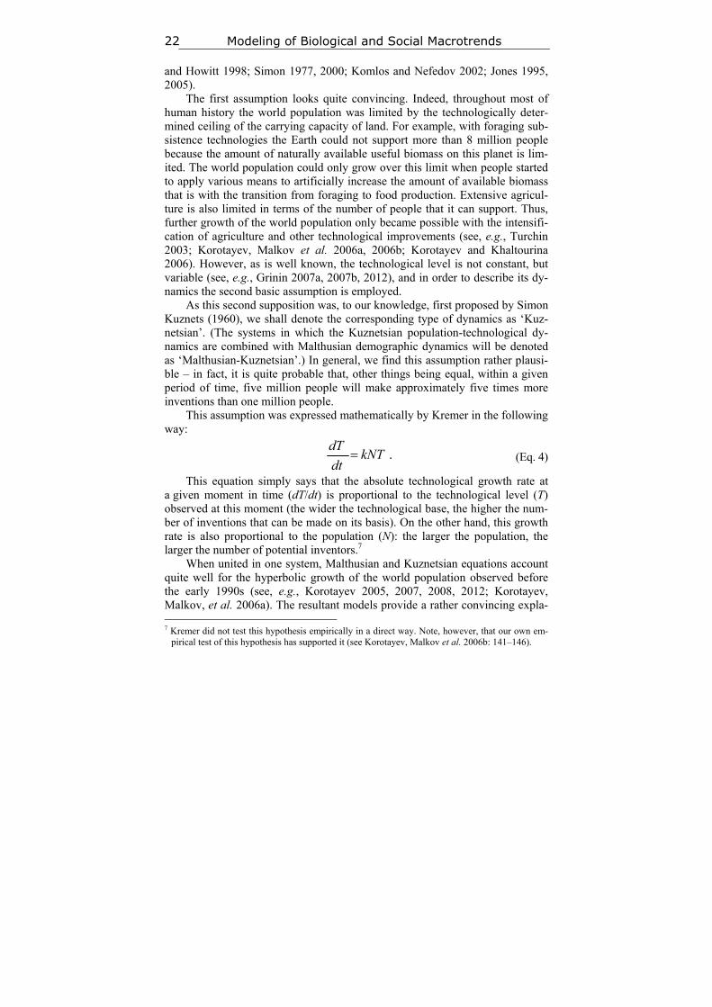
This assumption was expressed mathematically by Kremer in the following way:
.kNTdt
dT
(Eq. 4)
This equation simply says that the absolute technological growth rate at a given moment in time (dT/dt) is proportional to the technological level (T) observed at this moment (the wider the technological base, the higher the num-ber of inventions that can be made on its basis). On the other hand, this growth rate is also proportional to the population (N): the larger the population, the larger the number of potential inventors.7
When united in one system, Malthusian and Kuznetsian equations account quite well for the hyperbolic growth of the world population observed before the early 1990s (see, e.g., Korotayev 2005, 2007, 2008, 2012; Korotayev, Malkov, et al. 2006a). The resultant models provide a rather convincing expla- 7 Kremer did not test this hypothesis empirically in a direct way. Note, however, that our own em-
pirical test of this hypothesis has supported it (see Korotayev, Malkov et al. 2006b: 141–146).
Leonid E. Grinin, Alexander V. Markov, and Andrey V. Korotayev 23
nation of why, throughout most of human history, the world population fol-lowed the hyperbolic pattern with the absolute population growth rate tending to be proportional to N2. For example, why would the growth of population from, say, 10 million to 100 million, result in the growth of dN/dt 100 times? The above mentioned models explain this rather convincingly. The point is that the growth of world population from 10 to 100 million implies that human sub-sistence technologies also grew approximately 10 times (given that it will have proven, after all, to be able to support a population ten times larger). On the other hand, the tenfold population growth also implies a tenfold growth in the number of potential inventors, and, hence, a tenfold increase in the relative technological growth rate. Thus, the absolute technological growth rate would expand 10 × 10 = 100 times as, in accordance with Eq. 4, an order of magnitude higher number of people having at their disposal an order of magnitude wider technological base would tend to make two orders of magnitude more inven-tions. If, as throughout the Malthusian epoch, the world population (N) tended toward the technologically determined carrying capacity of the Earth, we have good reason to expect that dN/dt should also grow just by about 100 times.
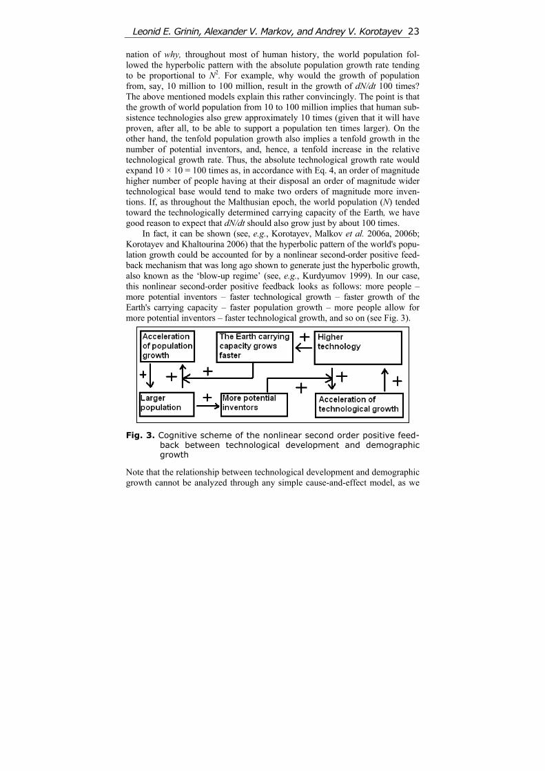
In fact, it can be shown (see, e.g., Korotayev, Malkov et al. 2006a, 2006b; Korotayev and Khaltourina 2006) that the hyperbolic pattern of the world's popu-lation growth could be accounted for by a nonlinear second-order positive feed-back mechanism that was long ago shown to generate just the hyperbolic growth, also known as the ‘blow-up regime’ (see, e.g., Kurdyumov 1999). In our case, this nonlinear second-order positive feedback looks as follows: more people – more potential inventors – faster technological growth – faster growth of the Earth's carrying capacity – faster population growth – more people allow for more potential inventors – faster technological growth, and so on (see Fig. 3).
Fig. 3. Cognitive scheme of the nonlinear second order positive feed-back between technological development and demographic growth
Note that the relationship between technological development and demographic growth cannot be analyzed through any simple cause-and-effect model, as we
Modeling of Biological and Social Macrotrends 24
observe a true dynamic relationship between these two processes – each of them is both the cause and the effect of the other.
The feedback system described here should be identified with the process of ‘collective learning’ described, principally, by Christian (2005: 146–148). The mathematical models of World System development discussed in this arti-cle can be interpreted as models of the influence that collective learning has on global social evolution (i.e., the evolution of the World System). Thus, the ra-ther peculiar hyperbolic shape of accelerated global development prior to the early 1970s may be regarded as a product of global collective learning. We have also shown (Korotayev, Malkov et al. 2006a: 34–66) that, for the period prior to the 1970s, World System economic and demographic macrodynamics, driven by the above-mentioned positive feedback loops, can simply and accu-rately be described with the following model:
,aSNdt
dN (Eq. 5)
.bNSdt
dS (Eq. 6)
The world GDP (G) can be calculated using the following equation: G = mN + SN, (Eq. 7)
where G is the world GDP, N is population, and S is the produced surplus per capita, over the subsistence amount (m) that is minimally necessary to repro-duce the population with a zero growth rate in a Malthusian system (thus, S = g – m, where g denotes per capita GDP); a and b are parameters.
The mathematical analysis of the basic model (not described here) suggests that up to the 1970s, the amount of S should be proportional, in the long run, to the World System's population: S = kN. Our statistical analysis of available empirical data has confirmed this theoretical proportionality (Korotayev, Malkov et al. 2006a: 49–50). Thus, in the right-hand side of Eq. 6, S can be replaced with kN, resulting in the following equation:
2kaNdt
dN .
Recall that the solution of this type of differential equations is:
)( 0 tt
CN t
,
which produces a simple hyperbolic curve. As, according to our model, S can be approximated as kN, its long-term
dynamics can be approximated with the following equation:
tt
kCS
0. (Eq. 8)
Leonid E. Grinin, Alexander V. Markov, and Andrey V. Korotayev 25
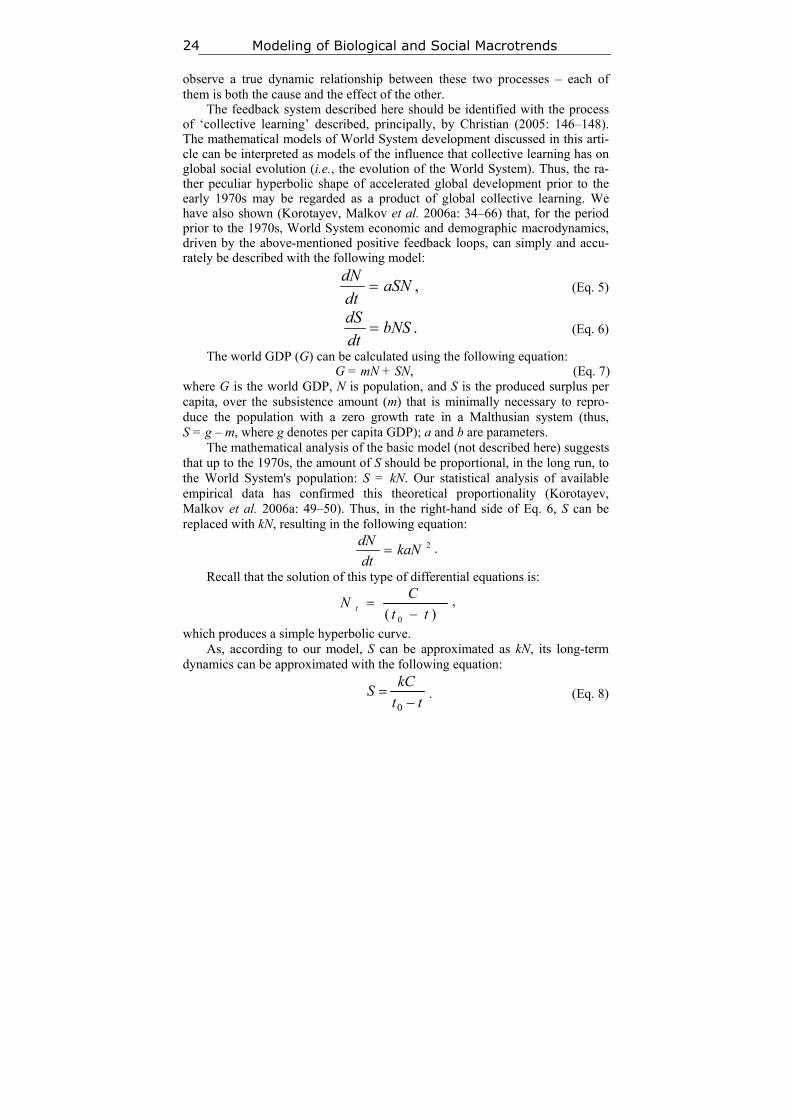
Thus, the long-term dynamics of the most dynamic component of the world GDP, SN, the ‘world surplus product’, can be approximated as follows:
20
2
tt
kCSN
. (Eq. 9)
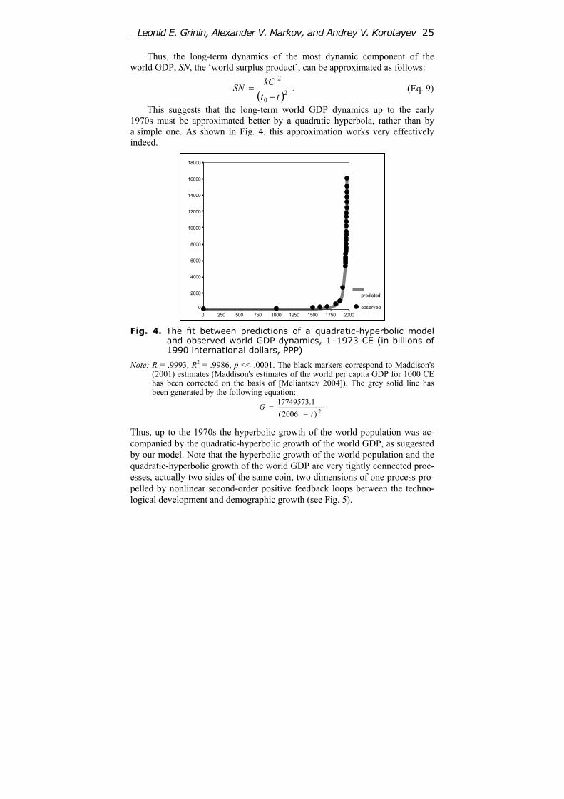
This suggests that the long-term world GDP dynamics up to the early 1970s must be approximated better by a quadratic hyperbola, rather than by a simple one. As shown in Fig. 4, this approximation works very effectively indeed.
Fig. 4. The fit between predictions of a quadratic-hyperbolic model and observed world GDP dynamics, 1–1973 CE (in billions of 1990 international dollars, PPP)
Note: R = .9993, R2 = .9986, p << .0001. The black markers correspond to Maddison's (2001) estimates (Maddison's estimates of the world per capita GDP for 1000 CE has been corrected on the basis of [Meliantsev 2004]). The grey solid line has been generated by the following equation:
2)2006(
17749573.1
tG
.
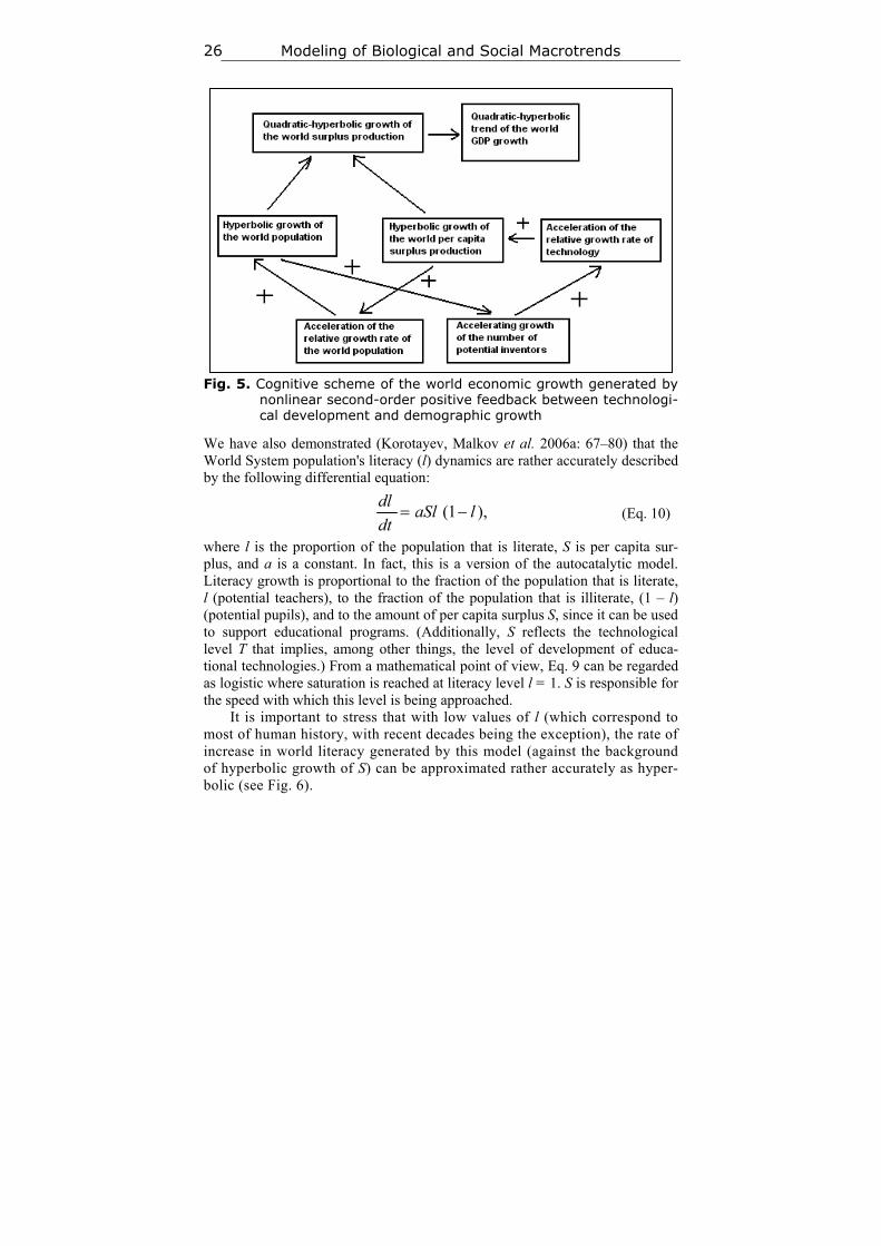
Thus, up to the 1970s the hyperbolic growth of the world population was ac-companied by the quadratic-hyperbolic growth of the world GDP, as suggested by our model. Note that the hyperbolic growth of the world population and the quadratic-hyperbolic growth of the world GDP are very tightly connected proc-esses, actually two sides of the same coin, two dimensions of one process pro-pelled by nonlinear second-order positive feedback loops between the techno-logical development and demographic growth (see Fig. 5).
200017501500125010007505002500
18000
16000
14000
12000
10000
8000
6000
4000
2000
0
predicted
observed
Modeling of Biological and Social Macrotrends 26
Fig. 5. Cognitive scheme of the world economic growth generated by nonlinear second-order positive feedback between technologi-cal development and demographic growth
We have also demonstrated (Korotayev, Malkov et al. 2006a: 67–80) that the World System population's literacy (l) dynamics are rather accurately described by the following differential equation:
),1( laSldt
dl (Eq. 10)
where l is the proportion of the population that is literate, S is per capita sur-plus, and a is a constant. In fact, this is a version of the autocatalytic model. Literacy growth is proportional to the fraction of the population that is literate, l (potential teachers), to the fraction of the population that is illiterate, (1 – l) (potential pupils), and to the amount of per capita surplus S, since it can be used to support educational programs. (Additionally, S reflects the technological level T that implies, among other things, the level of development of educa-tional technologies.) From a mathematical point of view, Eq. 9 can be regarded as logistic where saturation is reached at literacy level l = 1. S is responsible for the speed with which this level is being approached.
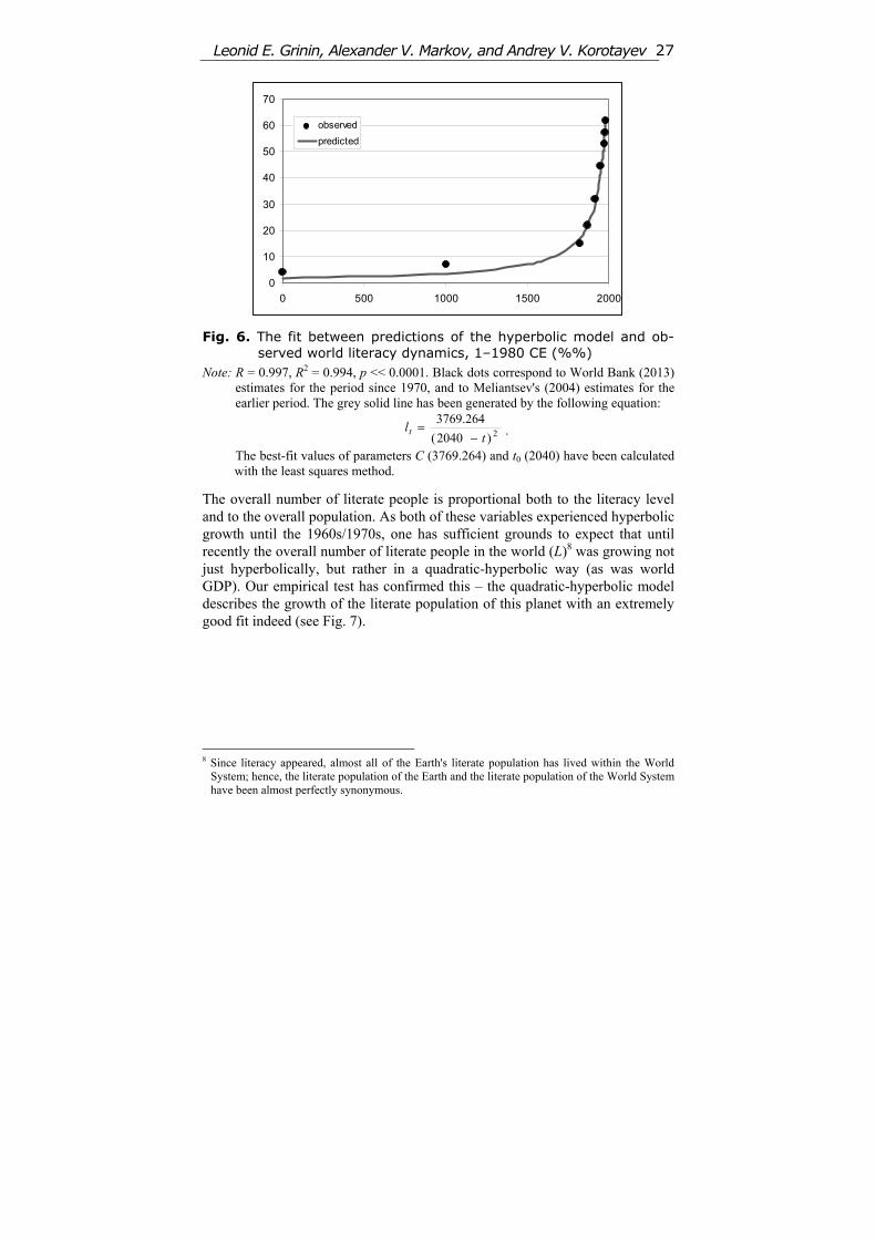
It is important to stress that with low values of l (which correspond to most of human history, with recent decades being the exception), the rate of increase in world literacy generated by this model (against the background of hyperbolic growth of S) can be approximated rather accurately as hyper-bolic (see Fig. 6).
Leonid E. Grinin, Alexander V. Markov, and Andrey V. Korotayev 27
Fig. 6. The fit between predictions of the hyperbolic model and ob-
served world literacy dynamics, 1–1980 CE (%%) Note: R = 0.997, R2 = 0.994, p << 0.0001. Black dots correspond to World Bank (2013)
estimates for the period since 1970, and to Meliantsev's (2004) estimates for the earlier period. The grey solid line has been generated by the following equation:
2)2040(
3769.264
tlt .
The best-fit values of parameters С (3769.264) and t0 (2040) have been calculated with the least squares method.
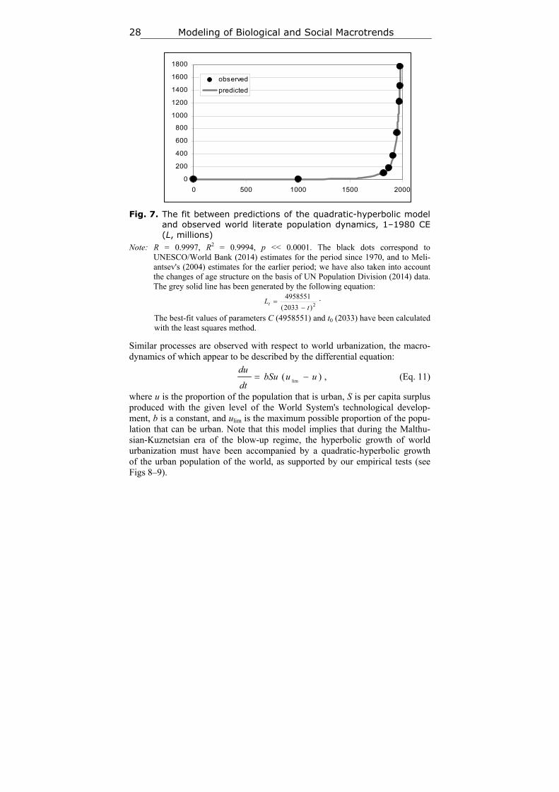
The overall number of literate people is proportional both to the literacy level and to the overall population. As both of these variables experienced hyperbolic growth until the 1960s/1970s, one has sufficient grounds to expect that until recently the overall number of literate people in the world (L)8 was growing not just hyperbolically, but rather in a quadratic-hyperbolic way (as was world GDP). Our empirical test has confirmed this – the quadratic-hyperbolic model describes the growth of the literate population of this planet with an extremely good fit indeed (see Fig. 7).
8 Since literacy appeared, almost all of the Earth's literate population has lived within the World
System; hence, the literate population of the Earth and the literate population of the World System have been almost perfectly synonymous.
0
10
20
30
40
50
60
70
0 500 1000 1500 2000
observed
predicted
Modeling of Biological and Social Macrotrends 28
Fig. 7. The fit between predictions of the quadratic-hyperbolic model
and observed world literate population dynamics, 1–1980 CE (L, millions)
Note: R = 0.9997, R2 = 0.9994, p << 0.0001. The black dots correspond to UNESCO/World Bank (2014) estimates for the period since 1970, and to Meli-antsev's (2004) estimates for the earlier period; we have also taken into account the changes of age structure on the basis of UN Population Division (2014) data. The grey solid line has been generated by the following equation:
2)2033(
4958551
tLt
.
The best-fit values of parameters С (4958551) and t0 (2033) have been calculated with the least squares method.
Similar processes are observed with respect to world urbanization, the macro-dynamics of which appear to be described by the differential equation:
)(lim
uubSudt
du , (Eq. 11)
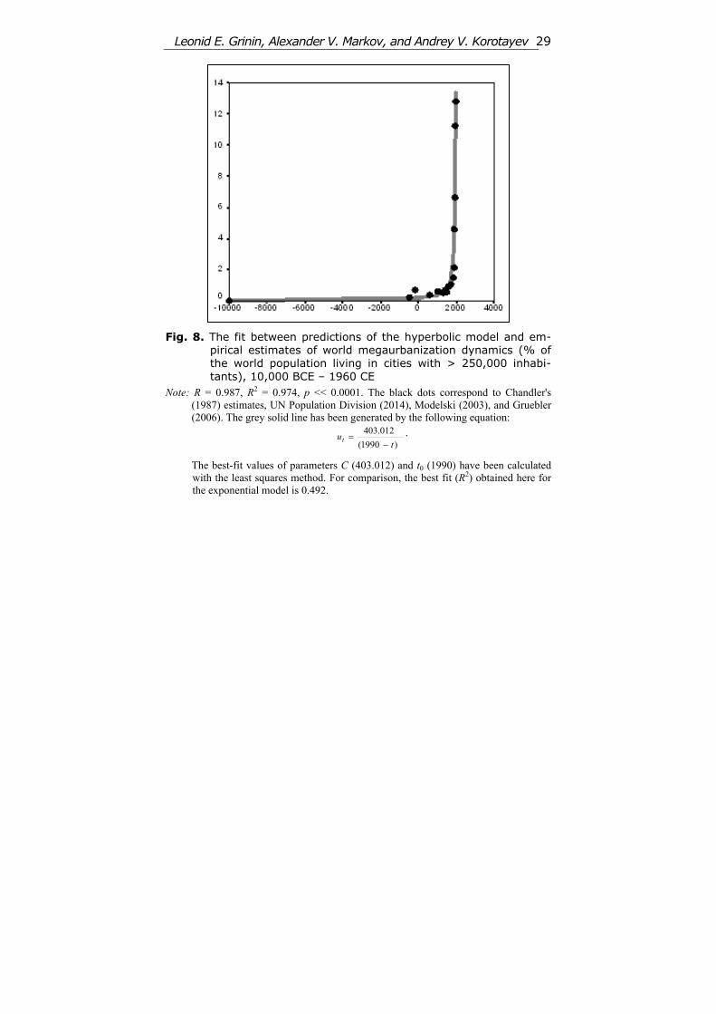
where u is the proportion of the population that is urban, S is per capita surplus produced with the given level of the World System's technological develop-ment, b is a constant, and ulim is the maximum possible proportion of the popu-lation that can be urban. Note that this model implies that during the Malthu-sian-Kuznetsian era of the blow-up regime, the hyperbolic growth of world urbanization must have been accompanied by a quadratic-hyperbolic growth of the urban population of the world, as supported by our empirical tests (see Figs 8–9).
0
200
400
600
800
1000
1200
1400
1600
1800
0 500 1000 1500 2000
observed
predicted
Leonid E. Grinin, Alexander V. Markov, and Andrey V. Korotayev 29
Fig. 8. The fit between predictions of the hyperbolic model and em-pirical estimates of world megaurbanization dynamics (% of the world population living in cities with > 250,000 inhabi-tants), 10,000 BCE – 1960 CE
Note: R = 0.987, R2 = 0.974, p << 0.0001. The black dots correspond to Chandler's (1987) estimates, UN Population Division (2014), Modelski (2003), and Gruebler (2006). The grey solid line has been generated by the following equation:
)1990(
403.012
tut
.
The best-fit values of parameters С (403.012) and t0 (1990) have been calculated with the least squares method. For comparison, the best fit (R2) obtained here for the exponential model is 0.492.
Modeling of Biological and Social Macrotrends 30
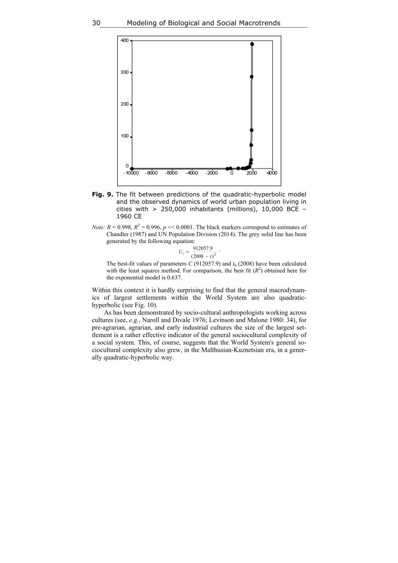
Fig. 9. The fit between predictions of the quadratic-hyperbolic model and the observed dynamics of world urban population living in cities with > 250,000 inhabitants (millions), 10,000 BCE – 1960 CE
Note: R = 0.998, R2 = 0.996, p << 0.0001. The black markers correspond to estimates of Chandler (1987) and UN Population Division (2014). The grey solid line has been generated by the following equation:
2)2008(
912057.9
tU t
.
The best-fit values of parameters С (912057.9) and t0 (2008) have been calculated with the least squares method. For comparison, the best fit (R2) obtained here for the exponential model is 0.637.
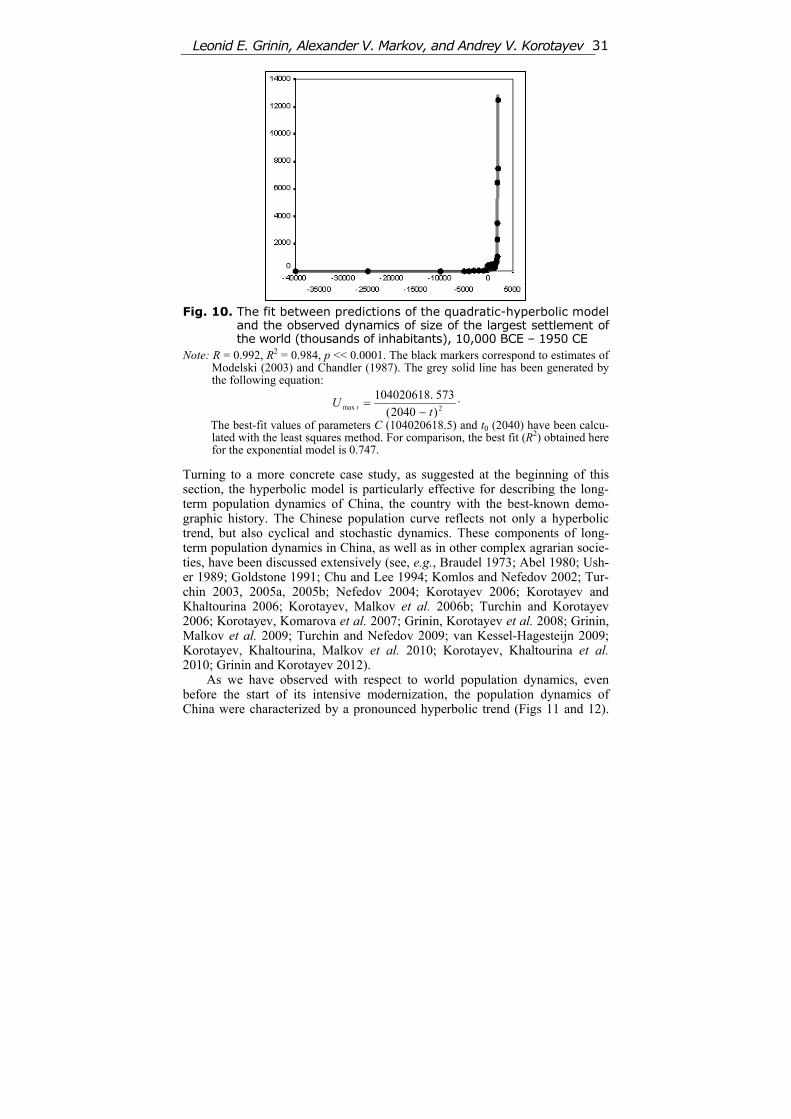
Within this context it is hardly surprising to find that the general macrodynam-ics of largest settlements within the World System are also quadratic-hyperbolic (see Fig. 10).
As has been demonstrated by socio-cultural anthropologists working across cultures (see, e.g., Naroll and Divale 1976; Levinson and Malone 1980: 34), for pre-agrarian, agrarian, and early industrial cultures the size of the largest set-tlement is a rather effective indicator of the general sociocultural complexity of a social system. This, of course, suggests that the World System's general so-ciocultural complexity also grew, in the Malthusian-Kuznetsian era, in a gener-ally quadratic-hyperbolic way.
Leonid E. Grinin, Alexander V. Markov, and Andrey V. Korotayev 31
Fig. 10. The fit between predictions of the quadratic-hyperbolic model
and the observed dynamics of size of the largest settlement of the world (thousands of inhabitants), 10,000 BCE – 1950 CE
Note: R = 0.992, R2 = 0.984, p << 0.0001. The black markers correspond to estimates of Modelski (2003) and Chandler (1987). The grey solid line has been generated by the following equation:
2max )2040(
573104020618.
tU t
.
The best-fit values of parameters С (104020618.5) and t0 (2040) have been calcu-lated with the least squares method. For comparison, the best fit (R2) obtained here for the exponential model is 0.747.
Turning to a more concrete case study, as suggested at the beginning of this section, the hyperbolic model is particularly effective for describing the long-term population dynamics of China, the country with the best-known demo-graphic history. The Chinese population curve reflects not only a hyperbolic trend, but also cyclical and stochastic dynamics. These components of long-term population dynamics in China, as well as in other complex agrarian socie-ties, have been discussed extensively (see, e.g., Braudel 1973; Abel 1980; Ush-er 1989; Goldstone 1991; Chu and Lee 1994; Komlos and Nefedov 2002; Tur-chin 2003, 2005a, 2005b; Nefedov 2004; Korotayev 2006; Korotayev and Khaltourina 2006; Korotayev, Malkov et al. 2006b; Turchin and Korotayev 2006; Korotayev, Komarova et al. 2007; Grinin, Korotayev et al. 2008; Grinin, Malkov et al. 2009; Turchin and Nefedov 2009; van Kessel-Hagesteijn 2009; Korotayev, Khaltourina, Malkov et al. 2010; Korotayev, Khaltourina et al. 2010; Grinin and Korotayev 2012).
As we have observed with respect to world population dynamics, even before the start of its intensive modernization, the population dynamics of China were characterized by a pronounced hyperbolic trend (Figs 11 and 12).
Modeling of Biological and Social Macrotrends 32
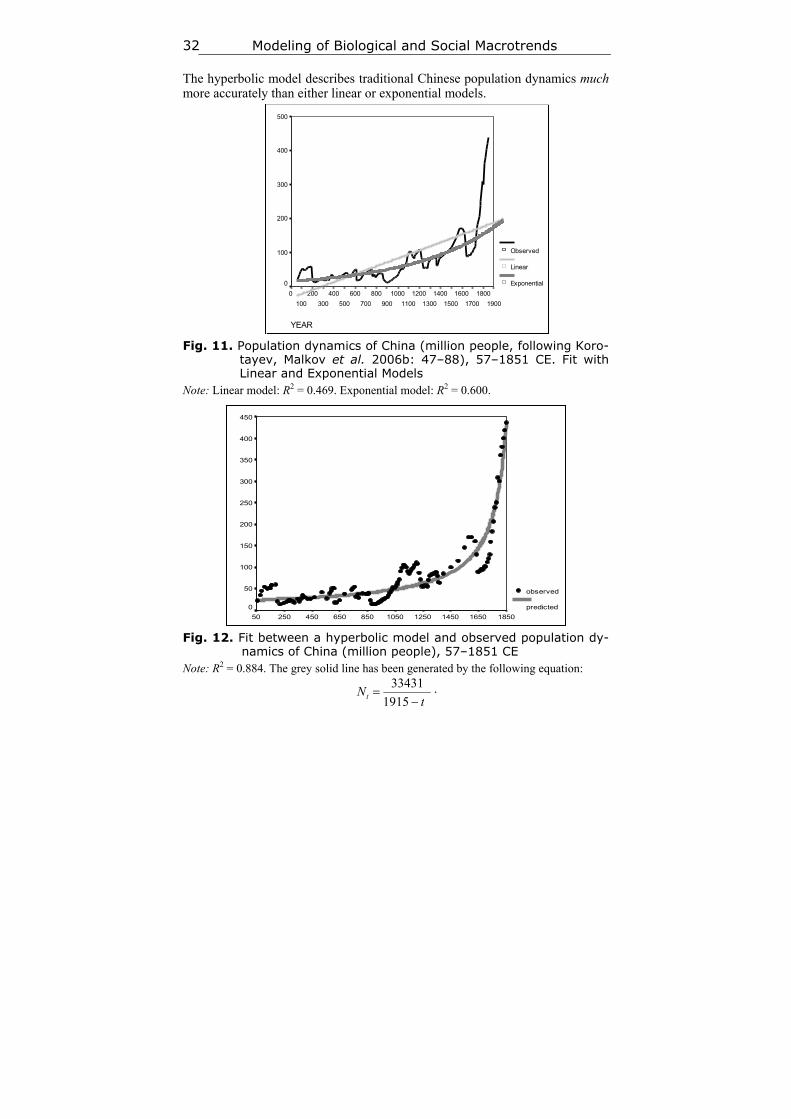
The hyperbolic model describes traditional Chinese population dynamics much more accurately than either linear or exponential models.
Fig. 11. Population dynamics of China (million people, following Koro-
tayev, Malkov et al. 2006b: 47–88), 57–1851 CE. Fit with Linear and Exponential Models
Note: Linear model: R2 = 0.469. Exponential model: R2 = 0.600.
Fig. 12. Fit between a hyperbolic model and observed population dy-
namics of China (million people), 57–1851 CE Note: R2 = 0.884. The grey solid line has been generated by the following equation:
tNt
1915
33431 .
YEAR
1900
1800
1700
1600
1500
1400
1300
1200
1100
1000
900
800
700
600
500
400
300
200
100
0
500
400
300
200
100
0
Observed
Linear
Exponential
1850165014501250105085065045025050
450
400
350
300
250
200
150
100
50
0
observed
predicted
Leonid E. Grinin, Alexander V. Markov, and Andrey V. Korotayev 33
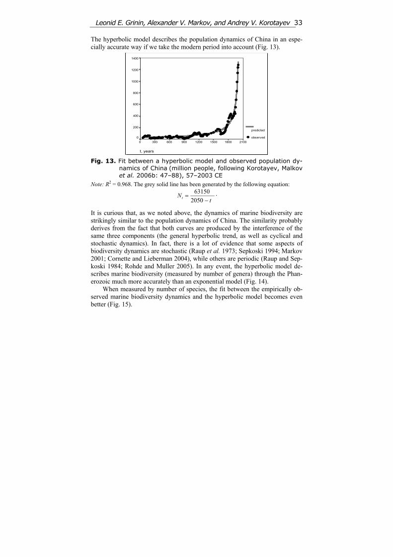
The hyperbolic model describes the population dynamics of China in an espe-cially accurate way if we take the modern period into account (Fig. 13).
Fig. 13. Fit between a hyperbolic model and observed population dy-
namics of China (million people, following Korotayev, Malkov et al. 2006b: 47–88), 57–2003 CE
Note: R2 = 0.968. The grey solid line has been generated by the following equation:
tNt
2050
63150 .
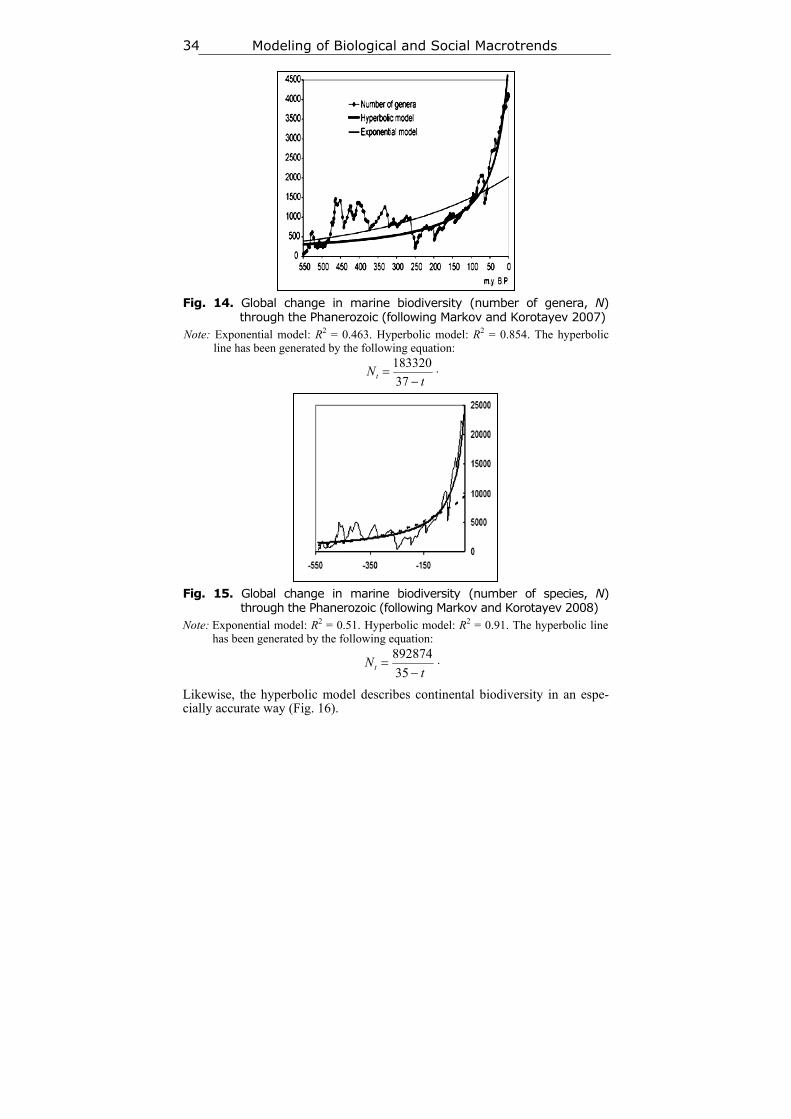
It is curious that, as we noted above, the dynamics of marine biodiversity are strikingly similar to the population dynamics of China. The similarity probably derives from the fact that both curves are produced by the interference of the same three components (the general hyperbolic trend, as well as cyclical and stochastic dynamics). In fact, there is a lot of evidence that some aspects of biodiversity dynamics are stochastic (Raup et al. 1973; Sepkoski 1994; Markov 2001; Cornette and Lieberman 2004), while others are periodic (Raup and Sep-koski 1984; Rohde and Muller 2005). In any event, the hyperbolic model de-scribes marine biodiversity (measured by number of genera) through the Phan-erozoic much more accurately than an exponential model (Fig. 14).
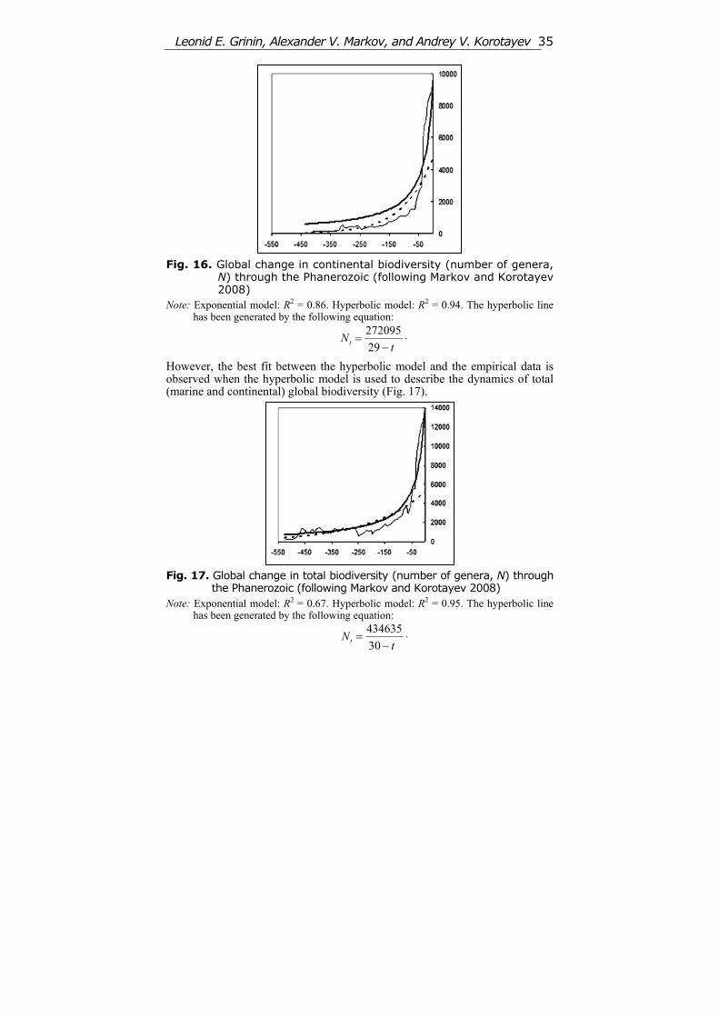
When measured by number of species, the fit between the empirically ob-served marine biodiversity dynamics and the hyperbolic model becomes even better (Fig. 15).
t, years
21001800150012009006003000
1400
1200
1000
800
600
400
200
0
predicted
observed
Modeling of Biological and Social Macrotrends 34
Fig. 14. Global change in marine biodiversity (number of genera, N)
through the Phanerozoic (following Markov and Korotayev 2007) Note: Exponential model: R2 = 0.463. Hyperbolic model: R2 = 0.854. The hyperbolic
line has been generated by the following equation:
tNt
37
183320 .
Fig. 15. Global change in marine biodiversity (number of species, N)
through the Phanerozoic (following Markov and Korotayev 2008) Note: Exponential model: R2 = 0.51. Hyperbolic model: R2 = 0.91. The hyperbolic line
has been generated by the following equation:
tNt
35
892874 .
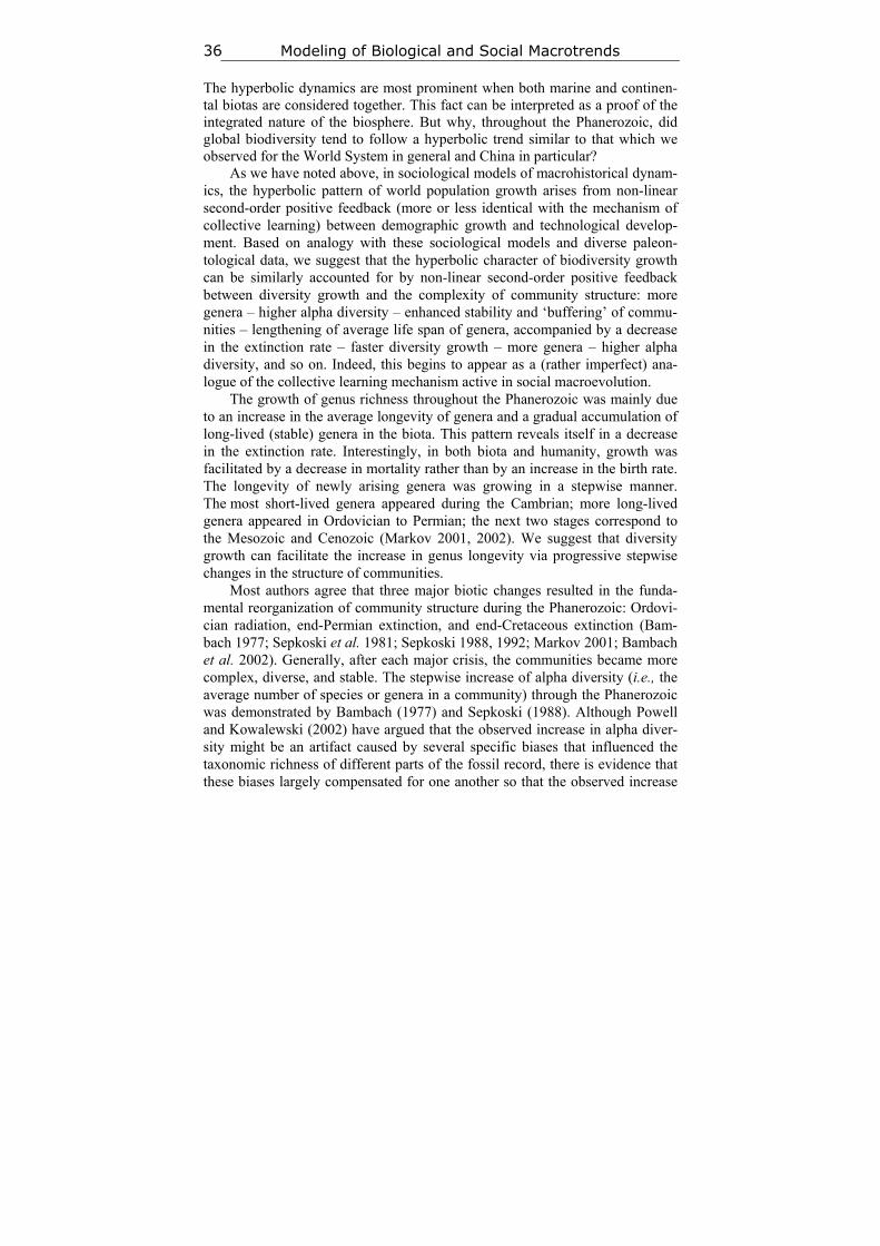
Likewise, the hyperbolic model describes continental biodiversity in an espe-cially accurate way (Fig. 16).
Leonid E. Grinin, Alexander V. Markov, and Andrey V. Korotayev 35
Fig. 16. Global change in continental biodiversity (number of genera,
N) through the Phanerozoic (following Markov and Korotayev 2008)
Note: Exponential model: R2 = 0.86. Hyperbolic model: R2 = 0.94. The hyperbolic line has been generated by the following equation:
tNt
29
272095 .
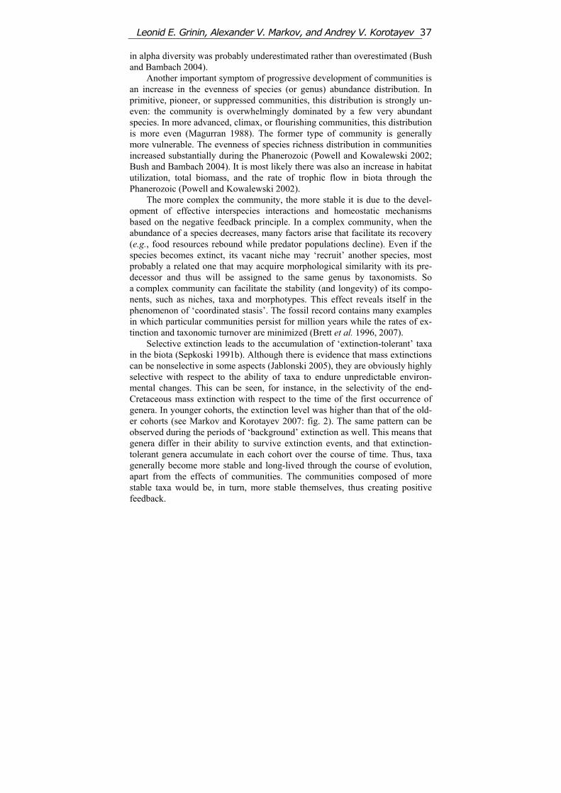
However, the best fit between the hyperbolic model and the empirical data is observed when the hyperbolic model is used to describe the dynamics of total (marine and continental) global biodiversity (Fig. 17).
Fig. 17. Global change in total biodiversity (number of genera, N) through
the Phanerozoic (following Markov and Korotayev 2008) Note: Exponential model: R2 = 0.67. Hyperbolic model: R2 = 0.95. The hyperbolic line
has been generated by the following equation:
tNt
30
434635 .
Modeling of Biological and Social Macrotrends 36
The hyperbolic dynamics are most prominent when both marine and continen-tal biotas are considered together. This fact can be interpreted as a proof of the integrated nature of the biosphere. But why, throughout the Phanerozoic, did global biodiversity tend to follow a hyperbolic trend similar to that which we observed for the World System in general and China in particular?
As we have noted above, in sociological models of macrohistorical dynam-ics, the hyperbolic pattern of world population growth arises from non-linear second-order positive feedback (more or less identical with the mechanism of collective learning) between demographic growth and technological develop-ment. Based on analogy with these sociological models and diverse paleon-tological data, we suggest that the hyperbolic character of biodiversity growth can be similarly accounted for by non-linear second-order positive feedback between diversity growth and the complexity of community structure: more genera – higher alpha diversity – enhanced stability and ‘buffering’ of commu-nities – lengthening of average life span of genera, accompanied by a decrease in the extinction rate – faster diversity growth – more genera – higher alpha diversity, and so on. Indeed, this begins to appear as a (rather imperfect) ana-logue of the collective learning mechanism active in social macroevolution.
The growth of genus richness throughout the Phanerozoic was mainly due to an increase in the average longevity of genera and a gradual accumulation of long-lived (stable) genera in the biota. This pattern reveals itself in a decrease in the extinction rate. Interestingly, in both biota and humanity, growth was facilitated by a decrease in mortality rather than by an increase in the birth rate. The longevity of newly arising genera was growing in a stepwise manner. The most short-lived genera appeared during the Cambrian; more long-lived genera appeared in Ordovician to Permian; the next two stages correspond to the Mesozoic and Cenozoic (Markov 2001, 2002). We suggest that diversity growth can facilitate the increase in genus longevity via progressive stepwise changes in the structure of communities.
Most authors agree that three major biotic changes resulted in the funda-mental reorganization of community structure during the Phanerozoic: Ordovi-cian radiation, end-Permian extinction, and end-Cretaceous extinction (Bam-bach 1977; Sepkoski et al. 1981; Sepkoski 1988, 1992; Markov 2001; Bambach et al. 2002). Generally, after each major crisis, the communities became more complex, diverse, and stable. The stepwise increase of alpha diversity (i.e., the average number of species or genera in a community) through the Phanerozoic was demonstrated by Bambach (1977) and Sepkoski (1988). Although Powell and Kowalewski (2002) have argued that the observed increase in alpha diver-sity might be an artifact caused by several specific biases that influenced the taxonomic richness of different parts of the fossil record, there is evidence that these biases largely compensated for one another so that the observed increase
Leonid E. Grinin, Alexander V. Markov, and Andrey V. Korotayev 37
in alpha diversity was probably underestimated rather than overestimated (Bush and Bambach 2004).
Another important symptom of progressive development of communities is an increase in the evenness of species (or genus) abundance distribution. In primitive, pioneer, or suppressed communities, this distribution is strongly un-even: the community is overwhelmingly dominated by a few very abundant species. In more advanced, climax, or flourishing communities, this distribution is more even (Magurran 1988). The former type of community is generally more vulnerable. The evenness of species richness distribution in communities increased substantially during the Phanerozoic (Powell and Kowalewski 2002; Bush and Bambach 2004). It is most likely there was also an increase in habitat utilization, total biomass, and the rate of trophic flow in biota through the Phanerozoic (Powell and Kowalewski 2002).
The more complex the community, the more stable it is due to the devel-opment of effective interspecies interactions and homeostatic mechanisms based on the negative feedback principle. In a complex community, when the abundance of a species decreases, many factors arise that facilitate its recovery (e.g., food resources rebound while predator populations decline). Even if the species becomes extinct, its vacant niche may ‘recruit’ another species, most probably a related one that may acquire morphological similarity with its pre-decessor and thus will be assigned to the same genus by taxonomists. So a complex community can facilitate the stability (and longevity) of its compo-nents, such as niches, taxa and morphotypes. This effect reveals itself in the phenomenon of ‘coordinated stasis’. The fossil record contains many examples in which particular communities persist for million years while the rates of ex-tinction and taxonomic turnover are minimized (Brett et al. 1996, 2007).
Selective extinction leads to the accumulation of ‘extinction-tolerant’ taxa in the biota (Sepkoski 1991b). Although there is evidence that mass extinctions can be nonselective in some aspects (Jablonski 2005), they are obviously highly selective with respect to the ability of taxa to endure unpredictable environ-mental changes. This can be seen, for instance, in the selectivity of the end-Cretaceous mass extinction with respect to the time of the first occurrence of genera. In younger cohorts, the extinction level was higher than that of the old-er cohorts (see Markov and Korotayev 2007: fig. 2). The same pattern can be observed during the periods of ‘background’ extinction as well. This means that genera differ in their ability to survive extinction events, and that extinction-tolerant genera accumulate in each cohort over the course of time. Thus, taxa generally become more stable and long-lived through the course of evolution, apart from the effects of communities. The communities composed of more stable taxa would be, in turn, more stable themselves, thus creating positive feedback.
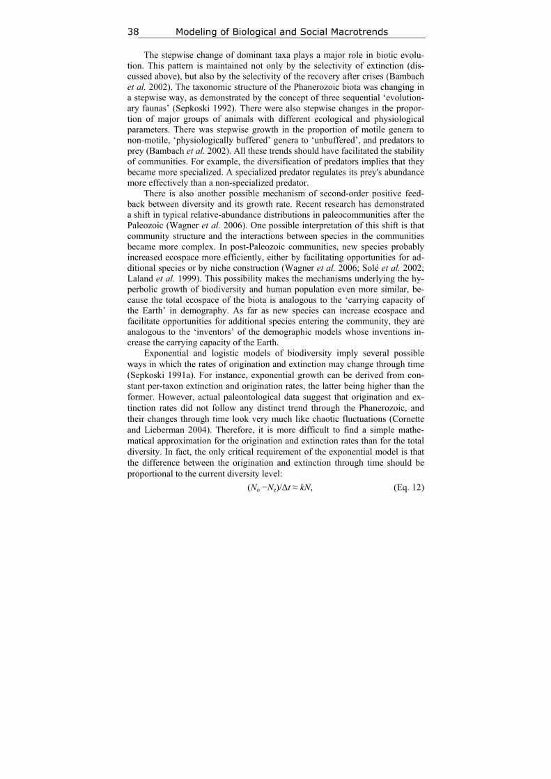
Modeling of Biological and Social Macrotrends 38
The stepwise change of dominant taxa plays a major role in biotic evolu-tion. This pattern is maintained not only by the selectivity of extinction (dis-cussed above), but also by the selectivity of the recovery after crises (Bambach et al. 2002). The taxonomic structure of the Phanerozoic biota was changing in a stepwise way, as demonstrated by the concept of three sequential ‘evolution-ary faunas’ (Sepkoski 1992). There were also stepwise changes in the propor-tion of major groups of animals with different ecological and physiological parameters. There was stepwise growth in the proportion of motile genera to non-motile, ‘physiologically buffered’ genera to ‘unbuffered’, and predators to prey (Bambach et al. 2002). All these trends should have facilitated the stability of communities. For example, the diversification of predators implies that they became more specialized. A specialized predator regulates its prey's abundance more effectively than a non-specialized predator.
There is also another possible mechanism of second-order positive feed-back between diversity and its growth rate. Recent research has demonstrated a shift in typical relative-abundance distributions in paleocommunities after the Paleozoic (Wagner et al. 2006). One possible interpretation of this shift is that community structure and the interactions between species in the communities became more complex. In post-Paleozoic communities, new species probably increased ecospace more efficiently, either by facilitating opportunities for ad-ditional species or by niche construction (Wagner et al. 2006; Solé et al. 2002; Laland et al. 1999). This possibility makes the mechanisms underlying the hy-perbolic growth of biodiversity and human population even more similar, be-cause the total ecospace of the biota is analogous to the ‘carrying capacity of the Earth’ in demography. As far as new species can increase ecospace and facilitate opportunities for additional species entering the community, they are analogous to the ‘inventors’ of the demographic models whose inventions in-crease the carrying capacity of the Earth.
Exponential and logistic models of biodiversity imply several possible ways in which the rates of origination and extinction may change through time (Sepkoski 1991a). For instance, exponential growth can be derived from con-stant per-taxon extinction and origination rates, the latter being higher than the former. However, actual paleontological data suggest that origination and ex-tinction rates did not follow any distinct trend through the Phanerozoic, and their changes through time look very much like chaotic fluctuations (Cornette and Lieberman 2004). Therefore, it is more difficult to find a simple mathe-matical approximation for the origination and extinction rates than for the total diversity. In fact, the only critical requirement of the exponential model is that the difference between the origination and extinction through time should be proportional to the current diversity level:
(No −Ne)/Δt ≈ kN, (Eq. 12)
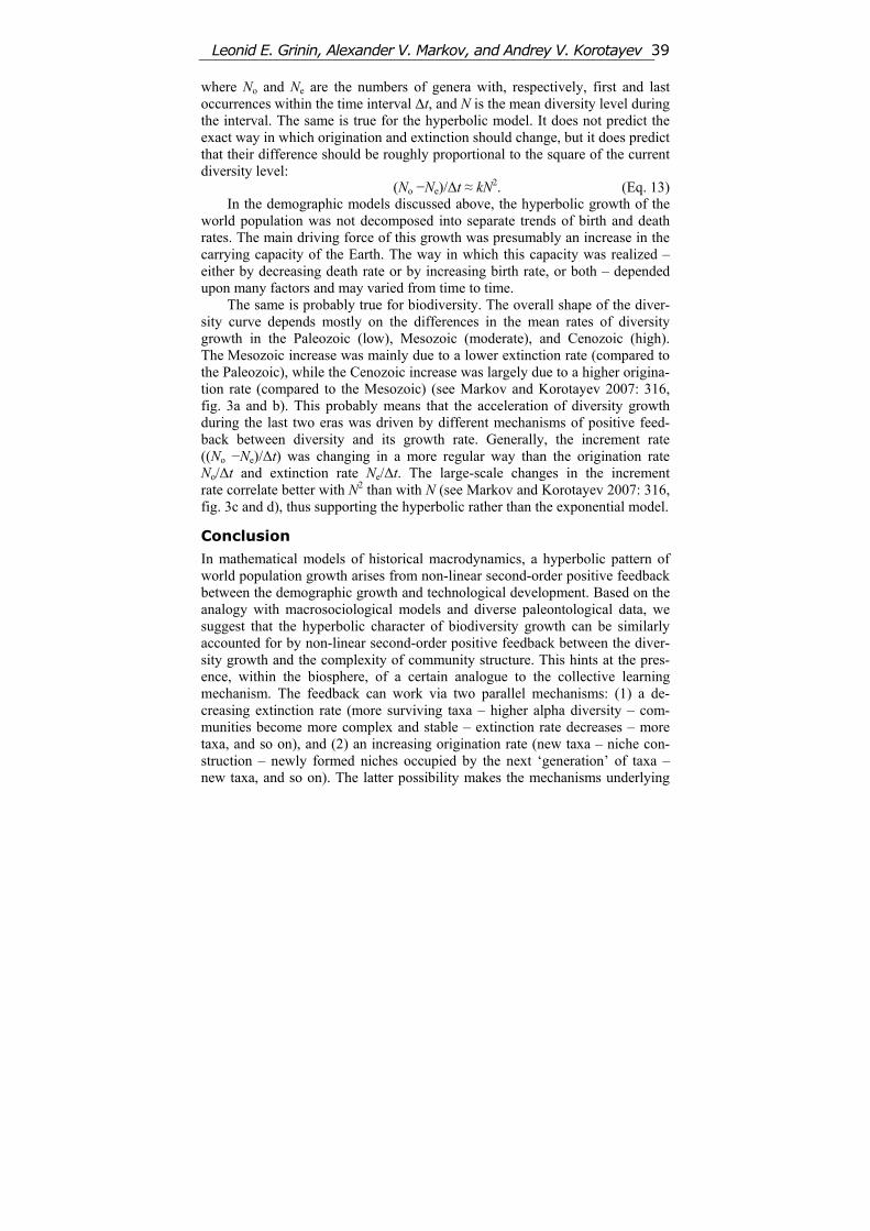
Leonid E. Grinin, Alexander V. Markov, and Andrey V. Korotayev 39
where No and Ne are the numbers of genera with, respectively, first and last occurrences within the time interval Δt, and N is the mean diversity level during the interval. The same is true for the hyperbolic model. It does not predict the exact way in which origination and extinction should change, but it does predict that their difference should be roughly proportional to the square of the current diversity level:
(No −Ne)/Δt ≈ kN2. (Eq. 13) In the demographic models discussed above, the hyperbolic growth of the
world population was not decomposed into separate trends of birth and death rates. The main driving force of this growth was presumably an increase in the carrying capacity of the Earth. The way in which this capacity was realized – either by decreasing death rate or by increasing birth rate, or both – depended upon many factors and may varied from time to time.
The same is probably true for biodiversity. The overall shape of the diver-sity curve depends mostly on the differences in the mean rates of diversity growth in the Paleozoic (low), Mesozoic (moderate), and Cenozoic (high). The Mesozoic increase was mainly due to a lower extinction rate (compared to the Paleozoic), while the Cenozoic increase was largely due to a higher origina-tion rate (compared to the Mesozoic) (see Markov and Korotayev 2007: 316, fig. 3a and b). This probably means that the acceleration of diversity growth during the last two eras was driven by different mechanisms of positive feed-back between diversity and its growth rate. Generally, the increment rate ((No −Ne)/Δt) was changing in a more regular way than the origination rate No/Δt and extinction rate Ne/Δt. The large-scale changes in the increment rate correlate better with N2 than with N (see Markov and Korotayev 2007: 316, fig. 3c and d), thus supporting the hyperbolic rather than the exponential model.
Conclusion
In mathematical models of historical macrodynamics, a hyperbolic pattern of world population growth arises from non-linear second-order positive feedback between the demographic growth and technological development. Based on the analogy with macrosociological models and diverse paleontological data, we suggest that the hyperbolic character of biodiversity growth can be similarly accounted for by non-linear second-order positive feedback between the diver-sity growth and the complexity of community structure. This hints at the pres-ence, within the biosphere, of a certain analogue to the collective learning mechanism. The feedback can work via two parallel mechanisms: (1) a de-creasing extinction rate (more surviving taxa – higher alpha diversity – com-munities become more complex and stable – extinction rate decreases – more taxa, and so on), and (2) an increasing origination rate (new taxa – niche con-struction – newly formed niches occupied by the next ‘generation’ of taxa – new taxa, and so on). The latter possibility makes the mechanisms underlying
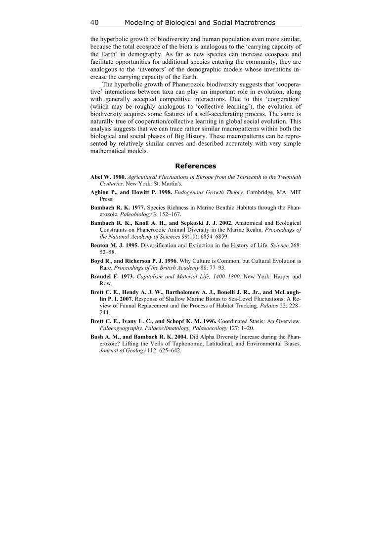
Modeling of Biological and Social Macrotrends 40
the hyperbolic growth of biodiversity and human population even more similar, because the total ecospace of the biota is analogous to the ‘carrying capacity of the Earth’ in demography. As far as new species can increase ecospace and facilitate opportunities for additional species entering the community, they are analogous to the ‘inventors’ of the demographic models whose inventions in-crease the carrying capacity of the Earth.
The hyperbolic growth of Phanerozoic biodiversity suggests that ‘coopera-tive’ interactions between taxa can play an important role in evolution, along with generally accepted competitive interactions. Due to this ‘cooperation’ (which may be roughly analogous to ‘collective learning’), the evolution of biodiversity acquires some features of a self-accelerating process. The same is naturally true of cooperation/collective learning in global social evolution. This analysis suggests that we can trace rather similar macropatterns within both the biological and social phases of Big History. These macropatterns can be repre-sented by relatively similar curves and described accurately with very simple mathematical models.
References
Abel W. 1980. Agricultural Fluctuations in Europe from the Thirteenth to the Twentieth Centuries. New York: St. Martin's.
Aghion P., and Howitt P. 1998. Endogenous Growth Theory. Cambridge, MA: MIT Press.
Bambach R. K. 1977. Species Richness in Marine Benthic Habitats through the Phan-erozoic. Paleobiology 3: 152–167.
Bambach R. K., Knoll A. H., and Sepkoski J. J. 2002. Anatomical and Ecological Constraints on Phanerozoic Animal Diversity in the Marine Realm. Proceedings of the National Academy of Sciences 99(10): 6854–6859.
Benton M. J. 1995. Diversification and Extinction in the History of Life. Science 268: 52–58.
Boyd R., and Richerson P. J. 1996. Why Culture is Common, but Cultural Evolution is Rare. Proceedings of the British Academy 88: 77–93.
Braudel F. 1973. Capitalism and Material Life, 1400–1800. New York: Harper and Row.
Brett C. E., Hendy A. J. W., Bartholomew A. J., Bonelli J. R., Jr., and McLaugh-lin P. I. 2007. Response of Shallow Marine Biotas to Sea-Level Fluctuations: A Re-view of Faunal Replacement and the Process of Habitat Tracking. Palaios 22: 228–244.
Brett C. E., Ivany L. C., and Schopf K. M. 1996. Coordinated Stasis: An Overview. Palaeogeography, Palaeoclimatology, Palaeoecology 127: 1–20.
Bush A. M., and Bambach R. K. 2004. Did Alpha Diversity Increase during the Phan-erozoic? Lifting the Veils of Taphonomic, Latitudinal, and Environmental Biases. Journal of Geology 112: 625–642.
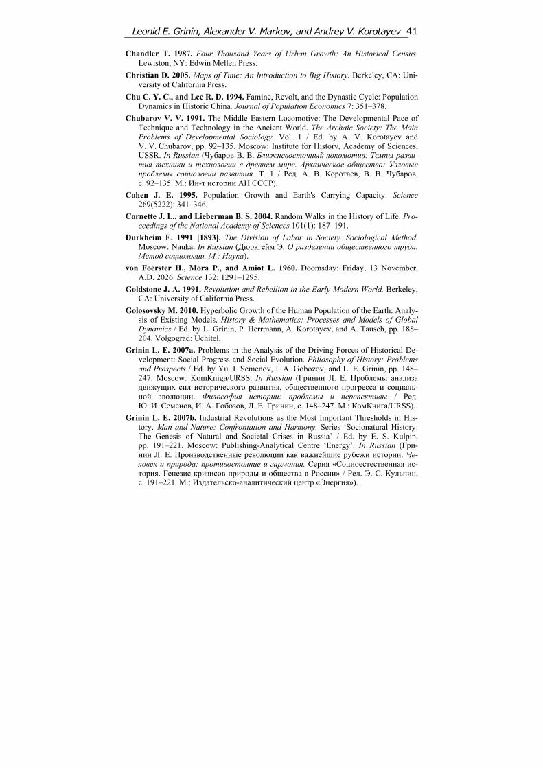
Leonid E. Grinin, Alexander V. Markov, and Andrey V. Korotayev 41
Chandler T. 1987. Four Thousand Years of Urban Growth: An Historical Census. Lewiston, NY: Edwin Mellen Press.
Christian D. 2005. Maps of Time: An Introduction to Big History. Berkeley, CA: Uni-versity of California Press.
Chu C. Y. C., and Lee R. D. 1994. Famine, Revolt, and the Dynastic Cycle: Population Dynamics in Historic China. Journal of Population Economics 7: 351–378.
Chubarov V. V. 1991. The Middle Eastern Locomotive: The Developmental Pace of Technique and Technology in the Ancient World. The Archaic Society: The Main Problems of Developmental Sociology. Vol. 1 / Ed. by A. V. Korotayev and V. V. Chubarov, pp. 92–135. Moscow: Institute for History, Academy of Sciences, USSR. In Russian (Чубаров В. В. Ближневосточный локомотив: Темпы разви-тия техники и технологии в древнем мире. Архаическое общество: Узловые проблемы социологии развития. Т. 1 / Ред. А. В. Коротаев, В. В. Чубаров, с. 92–135. М.: Ин-т истории АН СССР).
Cohen J. E. 1995. Population Growth and Earth's Carrying Capacity. Science 269(5222): 341–346.
Cornette J. L., and Lieberman B. S. 2004. Random Walks in the History of Life. Pro-ceedings of the National Academy of Sciences 101(1): 187–191.
Durkheim E. 1991 [1893]. The Division of Labor in Society. Sociological Method. Moscow: Nauka. In Russian (Дюркгейм Э. О разделении общественного труда. Метод социологии. М.: Наука).
von Foerster H., Mora P., and Amiot L. 1960. Doomsday: Friday, 13 November, A.D. 2026. Science 132: 1291–1295.
Goldstone J. A. 1991. Revolution and Rebellion in the Early Modern World. Berkeley, CA: University of California Press.
Golosovsky M. 2010. Hyperbolic Growth of the Human Population of the Earth: Analy-sis of Existing Models. History & Mathematics: Processes and Models of Global Dynamics / Ed. by L. Grinin, P. Herrmann, A. Korotayev, and A. Tausch, pp. 188–204. Volgograd: Uchitel.
Grinin L. E. 2007a. Problems in the Analysis of the Driving Forces of Historical De-velopment: Social Progress and Social Evolution. Philosophy of History: Problems and Prospects / Ed. by Yu. I. Semenov, I. A. Gobozov, and L. E. Grinin, pp. 148–247. Moscow: KomKniga/URSS. In Russian (Гринин Л. Е. Проблемы анализа движущих сил исторического развития, общественного прогресса и социаль-ной эволюции. Философия истории: проблемы и перспективы / Ред. Ю. И. Семенов, И. А. Гобозов, Л. Е. Гринин, с. 148–247. М.: КомКнига/URSS).
Grinin L. E. 2007b. Industrial Revolutions as the Most Important Thresholds in His-tory. Man and Nature: Confrontation and Harmony. Series ‘Socionatural History: The Genesis of Natural and Societal Crises in Russia’ / Ed. by E. S. Kulpin, pp. 191–221. Moscow: Publishing-Analytical Centre ‘Energy’. In Russian (Гри- нин Л. Е. Производственные революции как важнейшие рубежи истории. Че-ловек и природа: противостояние и гармония. Серия «Социоестественная ис-тория. Генезис кризисов природы и общества в России» / Ред. Э. С. Кульпин, с. 191–221. М.: Издательско-аналитический центр «Энергия»).
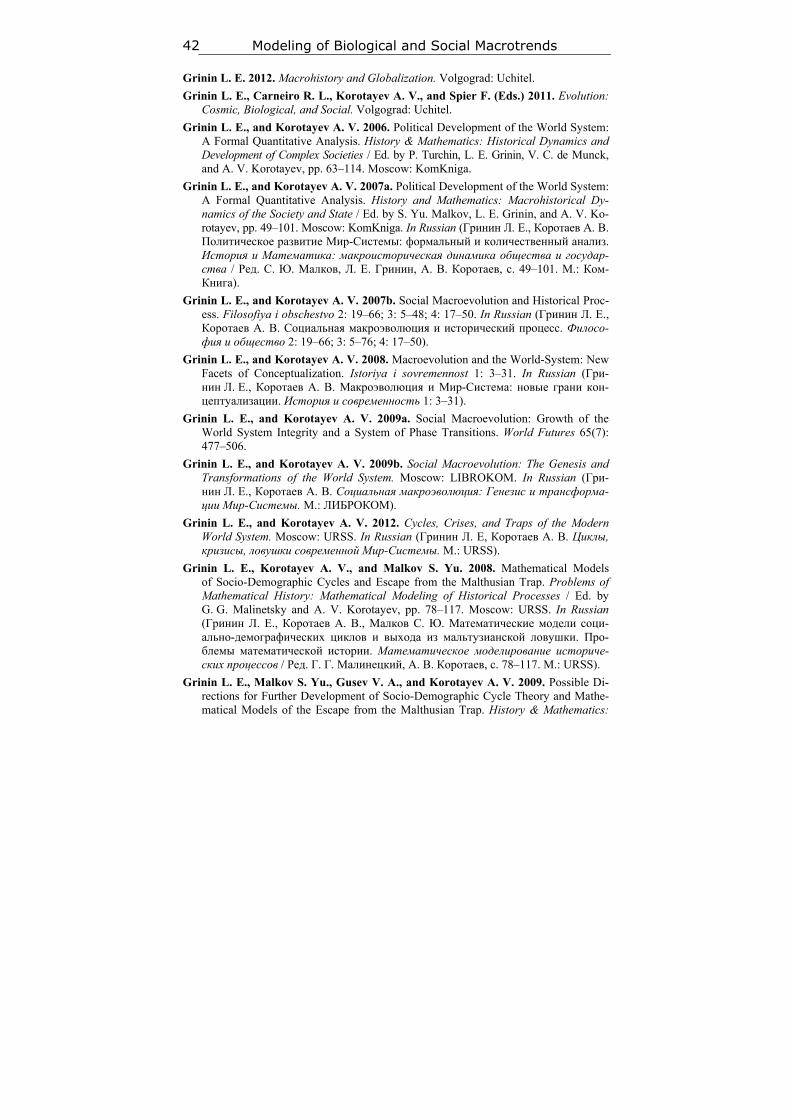
Modeling of Biological and Social Macrotrends 42
Grinin L. E. 2012. Macrohistory and Globalization. Volgograd: Uchitel.
Grinin L. E., Carneiro R. L., Korotayev A. V., and Spier F. (Eds.) 2011. Evolution: Cosmic, Biological, and Social. Volgograd: Uchitel.
Grinin L. E., and Korotayev A. V. 2006. Political Development of the World System: A Formal Quantitative Analysis. History & Mathematics: Historical Dynamics and Development of Complex Societies / Ed. by P. Turchin, L. E. Grinin, V. C. de Munck, and A. V. Korotayev, pp. 63–114. Moscow: KomKniga.
Grinin L. E., and Korotayev A. V. 2007a. Political Development of the World System: A Formal Quantitative Analysis. History and Mathematics: Macrohistorical Dy-namics of the Society and State / Ed. by S. Yu. Malkov, L. E. Grinin, and A. V. Ko-rotayev, pp. 49–101. Moscow: KomKniga. In Russian (Гринин Л. Е., Коротаев А. В. Политическое развитие Мир-Системы: формальный и количественный анализ. История и Математика: макроисторическая динамика общества и государ-ства / Ред. С. Ю. Малков, Л. Е. Гринин, А. В. Коротаев, с. 49–101. М.: Ком-Книга).
Grinin L. E., and Korotayev A. V. 2007b. Social Macroevolution and Historical Proc-ess. Filosofiya i obschestvo 2: 19–66; 3: 5–48; 4: 17–50. In Russian (Гринин Л. Е., Коротаев А. В. Социальная макроэволюция и исторический процесс. Филосо-фия и общество 2: 19–66; 3: 5–76; 4: 17–50).
Grinin L. E., and Korotayev A. V. 2008. Macroevolution and the World-System: New Facets of Conceptualization. Istoriya i sovremennost 1: 3–31. In Russian (Гри-нин Л. Е., Коротаев А. В. Макроэволюция и Мир-Система: новые грани кон-цептуализации. История и современность 1: 3–31).
Grinin L. E., and Korotayev A. V. 2009а. Social Macroevolution: Growth of the World System Integrity and a System of Phase Transitions. World Futures 65(7): 477–506.
Grinin L. E., and Korotayev A. V. 2009b. Social Macroevolution: The Genesis and Transformations of the World System. Moscow: LIBROKOM. In Russian (Гри-нин Л. Е., Коротаев А. В. Социальная макроэволюция: Генезис и трансформа-ции Мир-Системы. М.: ЛИБРОКОМ).
Grinin L. E., and Korotayev A. V. 2012. Cycles, Crises, and Traps of the Modern World System. Moscow: URSS. In Russian (Гринин Л. Е, Коротаев А. В. Циклы, кризисы, ловушки современной Мир-Системы. М.: URSS).
Grinin L. E., Korotayev A. V., and Malkov S. Yu. 2008. Mathematical Models of Socio-Demographic Cycles and Escape from the Malthusian Trap. Problems of Mathematical History: Mathematical Modeling of Historical Processes / Ed. by G. G. Malinetsky and A. V. Korotayev, pp. 78–117. Moscow: URSS. In Russian (Гринин Л. Е., Коротаев А. В., Малков С. Ю. Математические модели соци-ально-демографических циклов и выхода из мальтузианской ловушки. Про-блемы математической истории. Математическое моделирование историче-ских процессов / Ред. Г. Г. Малинецкий, А. В. Коротаев, с. 78–117. М.: URSS).
Grinin L. E., Malkov S. Yu., Gusev V. A., and Korotayev A. V. 2009. Possible Di-rections for Further Development of Socio-Demographic Cycle Theory and Mathe-matical Models of the Escape from the Malthusian Trap. History & Mathematics:
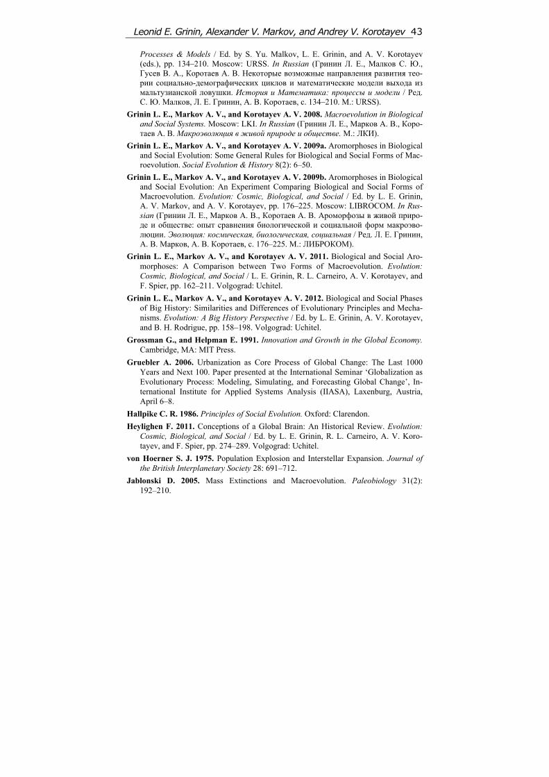
Leonid E. Grinin, Alexander V. Markov, and Andrey V. Korotayev 43
Processes & Models / Ed. by S. Yu. Malkov, L. E. Grinin, and A. V. Korotayev (eds.), pp. 134–210. Moscow: URSS. In Russian (Гринин Л. Е., Малков С. Ю., Гусев В. А., Коротаев А. В. Некоторые возможные направления развития тео-рии социально-демографических циклов и математические модели выхода из мальтузианской ловушки. История и Математика: процессы и модели / Ред. С. Ю. Малков, Л. Е. Гринин, А. В. Коротаев, с. 134–210. М.: URSS).
Grinin L. E., Markov A. V., and Korotayev A. V. 2008. Macroevolution in Biological and Social Systems. Мoscow: LKI. In Russian (Гринин Л. Е., Марков А. В., Коро-таев А. В. Макроэволюция в живой природе и обществе. М.: ЛКИ).
Grinin L. E., Markov A. V., and Korotayev A. V. 2009a. Aromorphoses in Biological and Social Evolution: Some General Rules for Biological and Social Forms of Mac-roevolution. Social Evolution & History 8(2): 6–50.
Grinin L. E., Markov A. V., and Korotayev A. V. 2009b. Aromorphoses in Biological and Social Evolution: An Experiment Comparing Biological and Social Forms of Macroevolution. Evolution: Cosmic, Biological, and Social / Ed. by L. E. Grinin, A. V. Markov, and A. V. Korotayev, pp. 176–225. Moscow: LIBROCOM. In Rus-sian (Гринин Л. Е., Марков А. В., Коротаев А. В. Ароморфозы в живой приро-де и обществе: опыт сравнения биологической и социальной форм макроэво-люции. Эволюция: космическая, биологическая, социальная / Ред. Л. Е. Гринин, А. В. Марков, А. В. Коротаев, с. 176–225. М.: ЛИБРОКОМ).
Grinin L. E., Markov A. V., and Korotayev A. V. 2011. Biological and Social Aro-morphoses: A Comparison between Two Forms of Macroevolution. Evolution: Cosmic, Biological, and Social / L. E. Grinin, R. L. Carneiro, A. V. Korotayev, and F. Spier, pp. 162–211. Volgograd: Uchitel.
Grinin L. E., Markov A. V., and Korotayev A. V. 2012. Biological and Social Phases of Big History: Similarities and Differences of Evolutionary Principles and Mecha-nisms. Evolution: A Big History Perspective / Ed. by L. E. Grinin, A. V. Korotayev, and B. H. Rodrigue, pp. 158–198. Volgograd: Uchitel.
Grossman G., and Helpman E. 1991. Innovation and Growth in the Global Economy. Cambridge, MA: MIT Press.
Gruebler A. 2006. Urbanization as Core Process of Global Change: The Last 1000 Years and Next 100. Paper presented at the International Seminar ‘Globalization as Evolutionary Process: Modeling, Simulating, and Forecasting Global Change’, In-ternational Institute for Applied Systems Analysis (IIASA), Laxenburg, Austria, April 6–8.
Hallpike C. R. 1986. Principles of Social Evolution. Oxford: Clarendon.
Heylighen F. 2011. Conceptions of a Global Brain: An Historical Review. Evolution: Cosmic, Biological, and Social / Ed. by L. E. Grinin, R. L. Carneiro, A. V. Koro-tayev, and F. Spier, pp. 274–289. Volgograd: Uchitel.
von Hoerner S. J. 1975. Population Explosion and Interstellar Expansion. Journal of the British Interplanetary Society 28: 691–712.
Jablonski D. 2005. Mass Extinctions and Macroevolution. Paleobiology 31(2): 192–210.
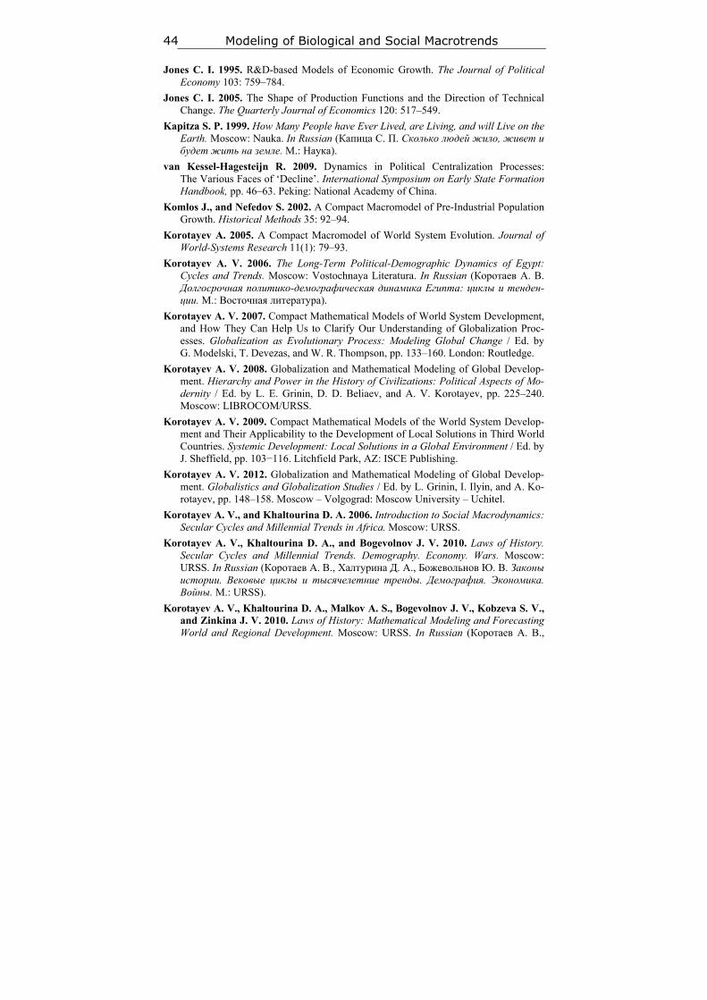
Modeling of Biological and Social Macrotrends 44
Jones C. I. 1995. R&D-based Models of Economic Growth. The Journal of Political Economy 103: 759–784.
Jones C. I. 2005. The Shape of Production Functions and the Direction of Technical Change. The Quarterly Journal of Economics 120: 517–549.
Kapitza S. P. 1999. How Many People have Ever Lived, are Living, and will Live on the Earth. Moscow: Nauka. In Russian (Капица С. П. Сколько людей жило, живет и будет жить на земле. М.: Наука).
van Kessel-Hagesteijn R. 2009. Dynamics in Political Centralization Processes: The Various Faces of ‘Decline’. International Symposium on Early State Formation Handbook, pp. 46–63. Peking: National Academy of China.
Komlos J., and Nefedov S. 2002. A Compact Macromodel of Pre-Industrial Population Growth. Historical Methods 35: 92–94.
Korotayev A. 2005. A Compact Macromodel of World System Evolution. Journal of World-Systems Research 11(1): 79–93.
Korotayev A. V. 2006. The Long-Term Political-Demographic Dynamics of Egypt: Cycles and Trends. Moscow: Vostochnaya Literatura. In Russian (Коротаев А. В. Долгосрочная политико-демографическая динамика Египта: циклы и тенден-ции. М.: Восточная литература).
Korotayev A. V. 2007. Compact Mathematical Models of World System Development, and How They Can Help Us to Clarify Our Understanding of Globalization Proc-esses. Globalization as Evolutionary Process: Modeling Global Change / Ed. by G. Modelski, T. Devezas, and W. R. Thompson, pp. 133–160. London: Routledge.
Korotayev A. V. 2008. Globalization and Mathematical Modeling of Global Develop-ment. Hierarchy and Power in the History of Civilizations: Political Aspects of Mo-dernity / Ed. by L. E. Grinin, D. D. Beliaev, and A. V. Korotayev, pp. 225–240. Moscow: LIBROCOM/URSS.
Korotayev A. V. 2009. Compact Mathematical Models of the World System Develop-ment and Their Applicability to the Development of Local Solutions in Third World Countries. Systemic Development: Local Solutions in a Global Environment / Ed. by J. Sheffield, pp. 103−116. Litchfield Park, AZ: ISCE Publishing.
Korotayev A. V. 2012. Globalization and Mathematical Modeling of Global Develop-ment. Globalistics and Globalization Studies / Ed. by L. Grinin, I. Ilyin, and A. Ko-rotayev, pp. 148–158. Moscow – Volgograd: Moscow University – Uchitel.
Korotayev A. V., and Khaltourina D. A. 2006. Introduction to Social Macrodynamics: Secular Cycles and Millennial Trends in Africa. Moscow: URSS.
Korotayev A. V., Khaltourina D. A., and Bogevolnov J. V. 2010. Laws of History. Secular Cycles and Millennial Trends. Demography. Economy. Wars. Moscow: URSS. In Russian (Коротаев А. В., Халтурина Д. А., Божевольнов Ю. В. Законы истории. Вековые циклы и тысячелетние тренды. Демография. Экономика. Войны. М.: URSS).
Korotayev A. V., Khaltourina D. A., Malkov A. S., Bogevolnov J. V., Kobzeva S. V., and Zinkina J. V. 2010. Laws of History: Mathematical Modeling and Forecasting World and Regional Development. Moscow: URSS. In Russian (Коротаев А. В.,
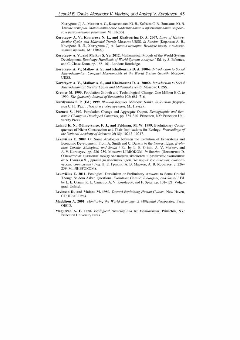
Leonid E. Grinin, Alexander V. Markov, and Andrey V. Korotayev 45
Халтурина Д. А., Малков А. С., Божевольнов Ю. В., Кобзева С. В., Зинькина Ю. В. Законы истории. Математическое моделирование и прогнозирование мирово-го и регионального развития. М.: URSS).
Korotayev A. V., Komarova N. L., and Khaltourina D. A. 2007. Laws of History: Secular Cycles and Millennial Trends. Moscow: URSS. In Russian (Коротаев А. В., Комарова Н. Л., Халтурина Д. А. Законы истории. Вековые циклы и тысяче-летние тренды. М.: URSS).
Korotayev A. V., and Malkov S. Yu. 2012. Mathematical Models of the World-System Development. Routledge Handbook of World-Systems Analysis / Ed. by S. Babones, and C. Chase-Dunn, pp. 158–161. London: Routledge.
Korotayev A. V., Malkov A. S., and Khaltourina D. A. 2006a. Introduction to Social Macrodynamics: Compact Macromodels of the World System Growth. Moscow: URSS.
Korotayev A. V., Malkov A. S., and Khaltourina D. A. 2006b. Introduction to Social Macrodynamics: Secular Cycles and Millennial Trends. Moscow: URSS.
Kremer M. 1993. Population Growth and Technological Change: One Million B.C. to 1990. The Quarterly Journal of Economics 108: 681–716.
Kurdyumov S. P. (Ed.) 1999. Blow-up Regimes. Moscow: Nauka. In Russian (Курдю-мов С. П. (Ред.). Режимы с обострением. М.: Наука).
Kuznets S. 1960. Population Change and Aggregate Output. Demographic and Eco-nomic Change in Developed Countries, pp. 324–340. Princeton, NY: Princeton Uni-versity Press.
Laland K. N., Odling-Smee, F. J., and Feldman, M. W. 1999. Evolutionary Conse-quences of Niche Construction and Their Implications for Ecology. Proceedings of the National Academy of Sciences 96(18): 10242–10247.
Lekevičius E. 2009. On Some Analogues between the Evolution of Ecosystems and Economic Development: From A. Smith and C. Darwin to the Newest Ideas. Evolu-tion: Cosmic, Biological, and Social / Ed. by L. E. Grinin, A. V. Markov, and A. V. Korotayev, pp. 226–259. Moscow: LIBROKOM. In Russian (Лекявичюс Э. О некоторых аналогиях между эволюцией экосистем и развитием экономики: от А. Смита и Ч. Дарвина до новейших идей. Эволюция: космическая, биологи-ческая, социальная / Ред. Л. Е. Гринин, А. В. Марков, А. В. Коротаев, с. 226–259. М.: ЛИБРОКОМ).
Lekevičius E. 2011. Ecological Darwinism or Preliminary Answers to Some Crucial Though Seldom Asked Questions. Evolution: Cosmic, Biological, and Social / Ed. by L. E. Grinin, R. L. Carneiro, A. V. Korotayev, and F. Spier, pp. 101–121. Volgo-grad: Uchitel.
Levinson D., and Malone M. 1980. Toward Explaining Human Culture. New Haven, CT: HRAF Press.
Maddison A. 2001. Monitoring the World Economy: A Millennial Perspective. Paris: OECD.
Magurran A. E. 1988. Ecological Diversity and Its Measurement. Princeton, NY: Princeton University Press.
Modeling of Biological and Social Macrotrends 46
Malthus T. 1978 [1798]. Population: The First Essay. Ann Arbor, MI: University of Michigan Press.
Markov A. V. 2001. Dynamics of the Marine Faunal Diversity in the Phanerozoic: A New Approach. Paleontological Journal 35: 1–9.
Markov A. V. 2002. Mechanisms Responsible for the Increase in the Taxonomic Diver-sity in the Phanerozoic Marine Biota. Paleontological Journal 36: 121–130.
Markov A. V., and Korotayev A. V. 2007. Phanerozoic Marine Biodiversity Follows a Hyperbolic Trend. Palaeoworld 16: 311–318.
Markov A. V., and Korotayev A. V. 2008. Hyperbolic Growth of Phanerozoic Marine and Continental Biodiversity. Zhurnal obshchey biologii 3: 175–194. In Russian (Марков А. В., Коротаев А. В. Гиперболический рост разнообразия морской и континентальной биот фанерозоя. Журнал общей биологии 3: 175–194).
Markov A. V., and Naymark E. B. 2009. On Some of the Newest Achievements in Evolutionary Biology. Evolution: Cosmic, Biological, and Social / Ed. by L. E. Gri- nin, A. V. Markov, and A. V. Korotayev, pp. 306–363. Moscow: LIBROCOM. In Russian (Марков А. В., Наймарк Е. Б. О некоторых новейших достижениях эволюционной биологии. Эволюция: космическая, биологическая, социальная / Ред. Л. Е. Гринин, А. В. Марков, А. В. Коротаев, с. 306–363. М.: ЛИБРОКОМ).
McEvedy C., and Jones R. 1978. Atlas of World Population History. New York: Facts on File.
Meliantsev V. A. 2004. Russia's Comparative Economic Development in the Long Run. Social Evolution & History 3(1): 106–136
Mesoudi A., Whiten A., and Laland K. 2006. Towards a Unified Science of Cultural Evolution. Behavioral and Brain Sciences 29: 329–383.
Modelski G. 2003. World Cities: –3000 to 2000. Washington: Faros2000.
Naroll R., and Divale W. T. 1976. Natural Selection in Cultural Evolution: Warfare versus Peaceful Diffusion. American Ethnologist 3: 97–128.
Nefedov S. A. 2004. A Model of Demographic Cycles in Traditional Societies: The Case of Ancient China. Social Evolution & History 3(1): 69–80.
Podlazov A. V. 2004. Theory of the Global Demographic Process. Mathematical Mod-eling of Social and Economic Dynamic / Ed. by M. G. Dmitriev, and A. P. Petrov, pp. 269–272. Moscow: Russian State Social University.
Powell M. G., and Kowalewski M. 2002. Increase in Evenness and Sampled Alpha Diversity through the Phanerozoic: Comparison of Early Paleozoic and Cenozoic Marine Fossil Assemblages. Geology 30(4): 331–334.
Raup D. M., Gould S. J., Schopf T. J. M., and Simberloff D. S. 1973. Stochastic Models of Phylogeny and the Evolution of Diversity. Journal of Geology 81(5): 525–542.
Raup D. M., and Sepkoski J. J. 1984. Periodicity of Extinctions in the Geologic Past. Proceedings of the National Academy of Sciences 81(3): 801–805.
Reeve H. K., and Hölldobler B. 2007. The Emergence of a Superorganism through Intergroup Competition. Proceedings of the National Academy of Sciences of the USA 104(23): 9736−9740.
Leonid E. Grinin, Alexander V. Markov, and Andrey V. Korotayev 47
Reznikova Zh. 2011. Evolutionary and Behavioural Aspects of Altruism in Animal Communities: Is There Room for Intelligence? Evolution: Cosmic, Biological, and Social / Ed. by L. E. Grinin, R. L. Carneiro, A. V. Korotayev, and F. Spier, pp. 162–211. Volgograd: Uchitel.
Robson S. K., and Traniello J. F. A. 2002. Transient Division of Labour and Behav-ioral Specialization in the Ant Formica Schaufussi. Naturwissenschaften 89: 128–131.
Rohde R. A., and Muller R. A. 2005. Cycles in Fossil Diversity. Nature 434(7030): 147–148.
Ryabko B., and Reznikova Zh. 2009. The Use of Ideas of Information Theory for Studying ‘Language’ and Intelligence in Ants. Entropy 11(4): 836–853.
Sepkoski J. J. 1988. Alpha, Beta or Gamma: Where Does All the Diversity Go? Paleo-biology 14: 221–234.
Sepkoski J. J. 1991a. Population Biology Models in Macroevolution. Analytical Paleo-biology. Short Courses in Paleontology. Vol. 4 / Ed. by N. L. Gilinsky, and P. W. Signor, pp. 136–156. Knoxville, TN: The Paleontological Society.
Sepkoski J. J. 1991b. Diversity in the Phanerozoic Oceans: A Partisan Review. The Unity of Evolutionary Biology / Ed. by E. C. Dudley, pp. 210–326. Portland, OR: Dioscorides Press.
Sepkoski J. J. 1992. Phylogenetic and Ecologic Patterns in the Phanerozoic History of Marine Biodiversity. Systematics, Ecology and the Biodiversity Crisis / Ed. by N. Eldredge, pp. 77–100. New York: Columbia University Press.
Sepkoski J. J. 1994. Limits to Randomness in Paleobiologic Models: The Case of Phanerozoic Species Diversity. Acta Palaeontologica Polonica 38(3–4): 174–198.
Sepkoski J. J., Bambach R. K., Raup D. M., and Valentine J. W. 1981. Phanerozoic Marine Diversity and the Fossil Record. Nature 293: 435–437.
Severtsov A. S. 1987. Criteria and Conditions for the Appearance of Aromorphic Or-ganization. Evolution and Biocenotic Crises / Ed. by L. P. Tatarinov, and A. P. Ras-nitsyn, pp. 64–76. Moscow: Nauka. In Russian (Северцов А. С. Критерии и усло-вия возникновения ароморфной организации. Эволюция и биоценотические кризисы / Ред. Л. П. Татаринов, А. П. Расницын, с. 64–76. М.: Наука).
Shmal'gauzen I. I. 1969. The Problems of Darwinism. Leningrad: Nauka. In Russian (Шмальгаузен И. И. Проблемы дарвинизма. Л.: Наука).
Simon J. 1977. The Economics of Population Growth. Princeton, NY: Princeton Uni-versity Press.
Simon J. 2000. The Great Breakthrough and Its Cause. Ann Arbor, MI: University of Michigan Press.
Solé R. V., Montoya J. M., and Erwin D. H. 2002. Recovery after Mass Extinction: Evolutionary Assembly in Large-Scale Biosphere Dynamics. Philosophical Trans-actions of the Royal Society of London, B 357: 697–707.
Spencer H. 1898. Principles of Sociology. Complete Work. Vol. 1. St. Petersburg: T-vo I. D. Sytina, Otd. N. A. Rubakina. In Russian (Спенсер Г. Основания социо-логии. Соч. Т. 1. СПб.: Т-во И. Д. Сытина, Отд. Н. А. Рубакина).
Modeling of Biological and Social Macrotrends 48
Taagapera R. 1976. Crisis around 2005 A.D.? A Technology-Population Interaction Model. General Systems 21: 137–138.
Taagapera R. 1979. People, Skills, and Resources: An Interaction Model for World Population Growth. Technological Forecasting and Social Change 13: 13–30.
Tsirel S. V. 2004. On the Possible Reasons for the Hyperexponential Growth of the Earth Population. Mathematical Modeling of Social and Economic Dynamics / Ed. by M. G. Dmitriev, and A. P. Petrov, pp. 367–369. Moscow: Russian State Social University.
Turchin P. 2003. Historical Dynamics: Why States Rise and Fall. Princeton, NY: Princeton University Press.
Turchin P. 2005a. Dynamical Feedbacks between Population Growth and Sociopoliti-cal Instability in Agrarian States. Structure and Dynamics 1(1). URL: http://eschol arship.org/uc/item/0d17g8g9.
Turchin P. 2005b. War and Peace and War: Life Cycles of Imperial Nations. New York: Pi Press.
Turchin P., and Korotayev A. 2006. Population Density and Warfare: A Reconsidera-tion. Social Evolution & History 5(2): 121–158.
Turchin P., and Nefedov S. 2009. Secular Cycles. Princeton, NY: Princeton University Press.
UN Population Division. 2014. United Nations Population Division database. URL: http://www.un.org/esa/population.
US Bureau of the Census. 2013. World Population Information. URL: http://www. census.gov/ipc /www/world.html.
Usher D. 1989. The Dynastic Cycle and the Stationary State. The American Economic Review 79: 1031–1044.
Wagner P. J., Kosnik M. A., and Lidgard S. 2006. Abundance Distributions Imply Elevated Complexity of Post-Paleozoic Marine Ecosystems. Science 314: 1289–1292.
World Bank. 2013. World Development Indicators Online. URL: http://data.world bank.org/indicator.
History & Mathematics: Trends and Cycles 2014 49–107
49
2
The World System Trajectory: The Reality of Constraints
and the Potential for Prediction
Tony Harper
Abstract
This paper discusses a number of constraints imposed on the trajectory of the World-System. Chief among these are the overall trend of the trajectory of the world system, the existence of lines of equal maximum urban area, that is iso-urban lines, constraints revealed by converting the trajectory to polar co-ordinates, periodic relationships within that representation, and the use of the ratio of observed maximum urban area to idealized maximum urban area to establish significant similarity with regard to two separate phases of urbaniza-tion including similarity in fractal dimensions of each phase. Beyond recogniz-ing this suite of constraints, their potential for prediction of the state or posi-tion of the world system is discussed.
Keywords: de-urbanization, fractal dimension, iso-urban lines, optimum urban area, parametric equation.
In the employing of mathematical methods, however, biological facts must be reduced to a mere abstract of their real complexity. It is im-portant to understand that this simplification is recognized for what it is: a working method. It does not mean to ignore the complexity and to-tality of biological relationships. These clearly remain the foundation upon which any mathe-matical model may be built.
C. C. Li, 1955
Acknowledgements
I wish to thank the following people for their comments and constructive criti-cisms: Andrey Korotayev, Sergey Tsirel, and Alexey Fomin. However, any errors or misinterpretations within the text of this paper are mine and mine alone. I wish to thank Kseniya Ukhova for her expert editorial hand.
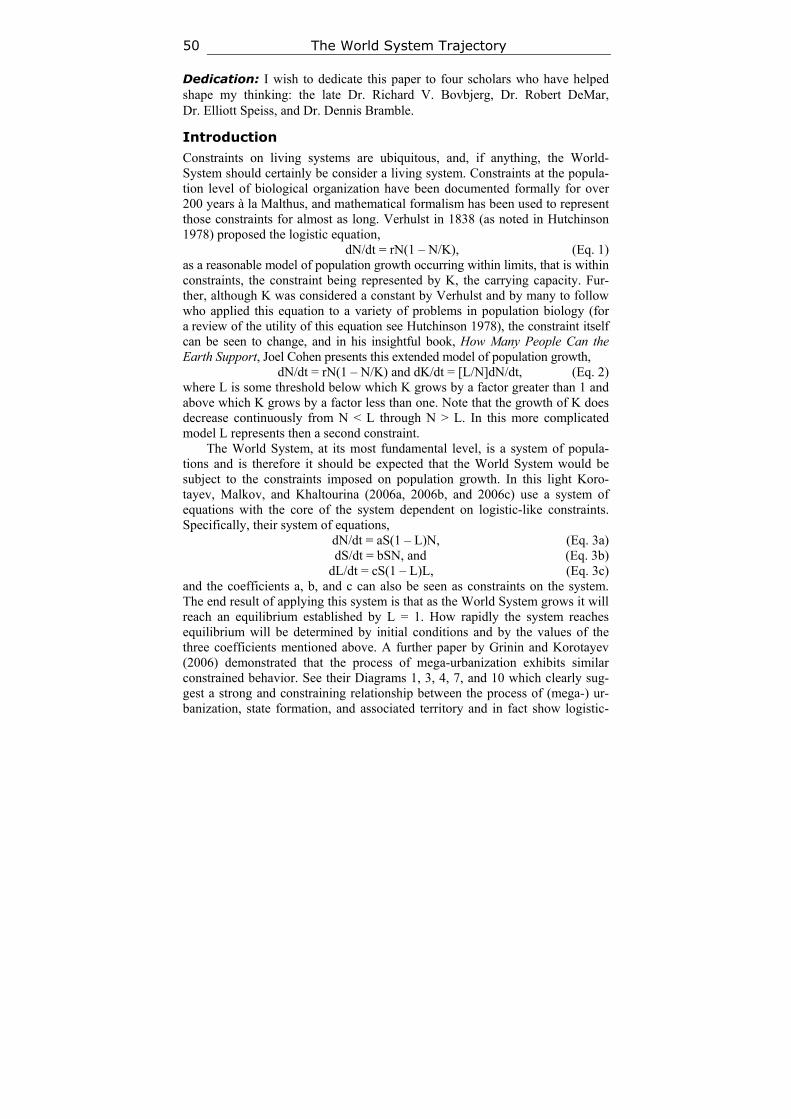
The World System Trajectory 50
Dedication: I wish to dedicate this paper to four scholars who have helped shape my thinking: the late Dr. Richard V. Bovbjerg, Dr. Robert DeMar, Dr. Elliott Speiss, and Dr. Dennis Bramble.
Introduction
Constraints on living systems are ubiquitous, and, if anything, the World-System should certainly be consider a living system. Constraints at the popula-tion level of biological organization have been documented formally for over 200 years à la Malthus, and mathematical formalism has been used to represent those constraints for almost as long. Verhulst in 1838 (as noted in Hutchinson 1978) proposed the logistic equation,
dN/dt = rN(1 – N/K), (Eq. 1) as a reasonable model of population growth occurring within limits, that is within constraints, the constraint being represented by K, the carrying capacity. Fur-ther, although K was considered a constant by Verhulst and by many to follow who applied this equation to a variety of problems in population biology (for a review of the utility of this equation see Hutchinson 1978), the constraint itself can be seen to change, and in his insightful book, How Many People Can the Earth Support, Joel Cohen presents this extended model of population growth,
dN/dt = rN(1 – N/K) and dK/dt = [L/N]dN/dt, (Eq. 2) where L is some threshold below which K grows by a factor greater than 1 and above which K grows by a factor less than one. Note that the growth of K does decrease continuously from N < L through N > L. In this more complicated model L represents then a second constraint.
The World System, at its most fundamental level, is a system of popula-tions and is therefore it should be expected that the World System would be subject to the constraints imposed on population growth. In this light Koro-tayev, Malkov, and Khaltourina (2006a, 2006b, and 2006c) use a system of equations with the core of the system dependent on logistic-like constraints. Specifically, their system of equations,
dN/dt = aS(1 – L)N, (Eq. 3a) dS/dt = bSN, and (Eq. 3b)
dL/dt = cS(1 – L)L, (Eq. 3c) and the coefficients a, b, and c can also be seen as constraints on the system. The end result of applying this system is that as the World System grows it will reach an equilibrium established by L = 1. How rapidly the system reaches equilibrium will be determined by initial conditions and by the values of the three coefficients mentioned above. A further paper by Grinin and Korotayev (2006) demonstrated that the process of mega-urbanization exhibits similar constrained behavior. See their Diagrams 1, 3, 4, 7, and 10 which clearly sug-gest a strong and constraining relationship between the process of (mega-) ur-banization, state formation, and associated territory and in fact show logistic-
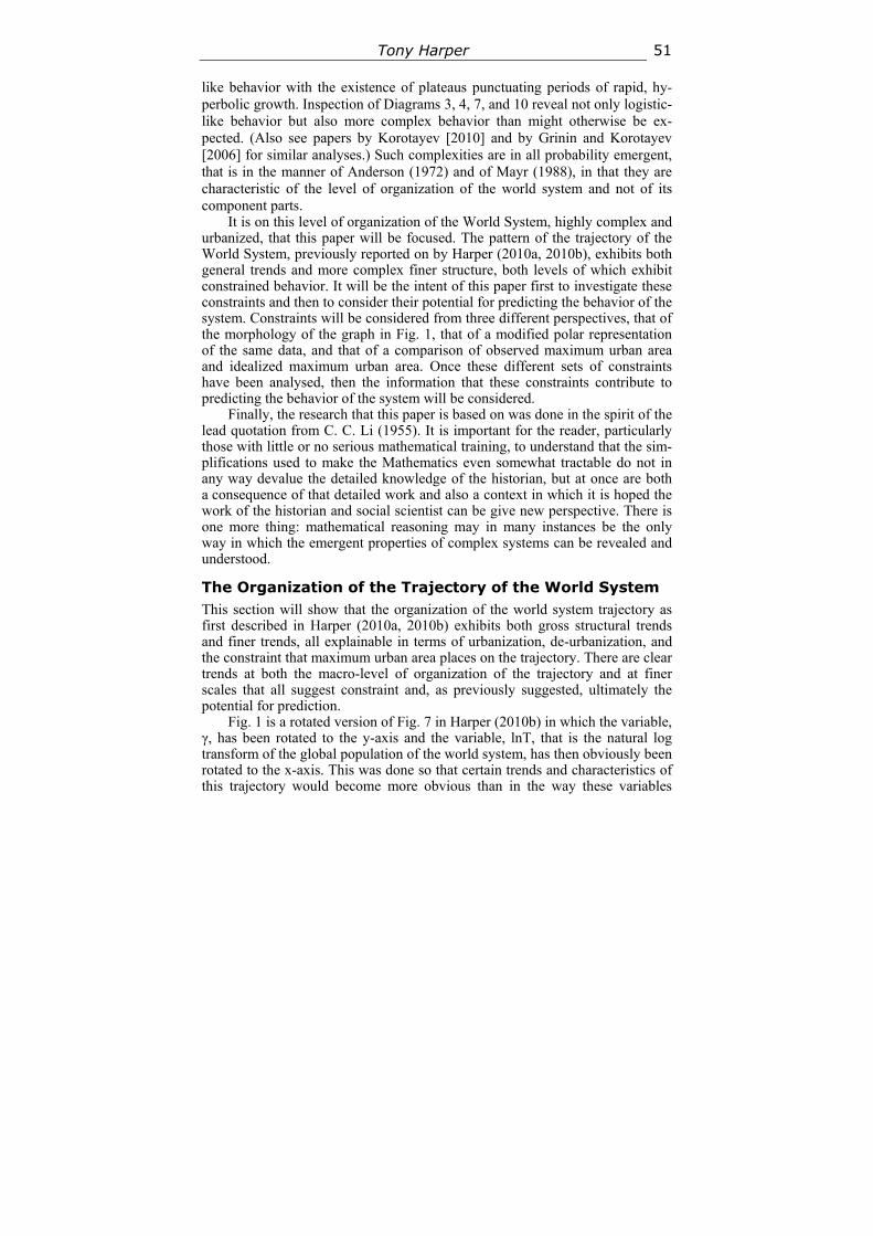
Tony Harper 51
like behavior with the existence of plateaus punctuating periods of rapid, hy-perbolic growth. Inspection of Diagrams 3, 4, 7, and 10 reveal not only logistic-like behavior but also more complex behavior than might otherwise be ex-pected. (Also see papers by Korotayev [2010] and by Grinin and Korotayev [2006] for similar analyses.) Such complexities are in all probability emergent, that is in the manner of Anderson (1972) and of Mayr (1988), in that they are characteristic of the level of organization of the world system and not of its component parts.
It is on this level of organization of the World System, highly complex and urbanized, that this paper will be focused. The pattern of the trajectory of the World System, previously reported on by Harper (2010a, 2010b), exhibits both general trends and more complex finer structure, both levels of which exhibit constrained behavior. It will be the intent of this paper first to investigate these constraints and then to consider their potential for predicting the behavior of the system. Constraints will be considered from three different perspectives, that of the morphology of the graph in Fig. 1, that of a modified polar representation of the same data, and that of a comparison of observed maximum urban area and idealized maximum urban area. Once these different sets of constraints have been analysed, then the information that these constraints contribute to predicting the behavior of the system will be considered.
Finally, the research that this paper is based on was done in the spirit of the lead quotation from C. C. Li (1955). It is important for the reader, particularly those with little or no serious mathematical training, to understand that the sim-plifications used to make the Mathematics even somewhat tractable do not in any way devalue the detailed knowledge of the historian, but at once are both a consequence of that detailed work and also a context in which it is hoped the work of the historian and social scientist can be give new perspective. There is one more thing: mathematical reasoning may in many instances be the only way in which the emergent properties of complex systems can be revealed and understood.
The Organization of the Trajectory of the World System This section will show that the organization of the world system trajectory as first described in Harper (2010a, 2010b) exhibits both gross structural trends and finer trends, all explainable in terms of urbanization, de-urbanization, and the constraint that maximum urban area places on the trajectory. There are clear trends at both the macro-level of organization of the trajectory and at finer scales that all suggest constraint and, as previously suggested, ultimately the potential for prediction.
Fig. 1 is a rotated version of Fig. 7 in Harper (2010b) in which the variable, γ, has been rotated to the y-axis and the variable, lnT, that is the natural log transform of the global population of the world system, has then obviously been rotated to the x-axis. This was done so that certain trends and characteristics of this trajectory would become more obvious than in the way these variables
The World System Trajectory 52
were originally displayed. In particular, some of the fine(r) scale characteristics are easier to understand, and this graphical representation also displays a non-obvious relationship between the two variables graphed and the natural log of maximum urban area size.
Fig. 1. lnT on the X-axis is graphed against γ on the y-axis
Fig. 2. The graph above is as in Fig. 1 but with a linear regression
imposed on the data. A linear regression of the data yields, γ = –.0465lnT + 2.2607, representing an inverse relationship between γ and lnT. R2 = .5225
It can be seen by inspection of Fig. 1 that there is an inverse relationship be-tween γ and lnT, since over the full range of lnT γ decreases from an initial value of 1.4851 to a final value of 1.2099, a difference of .2752 or a decrease of 18.53 % of the initial value of γ. Further, the largest values of γ occur with low values of lnT, for example, when γ = 1.5674, its largest value, the value of lnT
Tony Harper 53
is 17.1731, which is an increase of 4.37 % over the initial value of lnT, while the largest value of lnT, 22.5478, is an increase of 37.03 % of the initial value of lnT. Perhaps, an easier and more general method of demonstrating this trend of decreasing γ with respect to lnT would be to generate a linear regression of this data. This is done in Fig. 2, yielding the regression equation,
γ = 2.23 – .0449lnT, (Eq. 4) and the fit of this equation is quite good with r = –.708 and the RMSE = .0593. The fact that this equation has a negative slope clearly shows that the overall trend of the world system is one of decreasing γ with increasing lnT. What does this general trend imply?
Decreasing γ implies increasing urbanization. By establishing a fixed value of C, that is Ca, with respect to Cmax, a defined section of the triangular area bounded by the natural log transform of the equation,
F = αC–γ (Eq. 5) can be arbitrarily defined as a boundary between urbanized and non-urbanized regions of the world system at a given time. By then holding A, the area bound-ed by
lnF = lnα – γlnC, (Eq. 6) constant and reducing γ it can be shown that the subsection of A bounded by Ca is greater than the subsection bounded by the original value of γ, and conse-quently represents an increase in urbanization. Note, that for any given time it can be shown that the ratio of urbanized to non-urbanized portions of the world system is given by:
U = (lnCm + x – lnCc)2/(lnCm + x)2. (Eq. 7)
As γ decreases with increasing lnT as represented by Eq. 4, it then follows that urbanization increases with increasing lnT. Modelski (2003) and Koro-tayev and Grinin (2006) have shown that urbanization has increased over time with the increase being punctuated by plateau-like phases and these phases ap-pear to be synchronized with a similar pattern in global population, here labeled as T. It is a contention of this paper that the increasing population of the world system is dependent on increasing urbanization and would not occur without the process of urbanization and in turn its attendant process of technological progress.
Within this broad trend of decreasing gamma, increasing lnT and therefore T, and increasing urbanization are micro-trends only the average of which is reflected by these broad trends. While a detailed analysis, on a century by cen-tury basis, will not be entered into here, two significant micro-trends will be mentioned, the period from 400 BCE to 700 CE, essentially the formation, flo-rescence, and demise of Rome, of the Han Empires and the mosaic of empires to follow the Han through to the establishment of the Tang Empire, and the origination of the Islamic Caliphates, and then the 12th to the 14th centuries CE. These two periods of time are significant, because they represent periods of
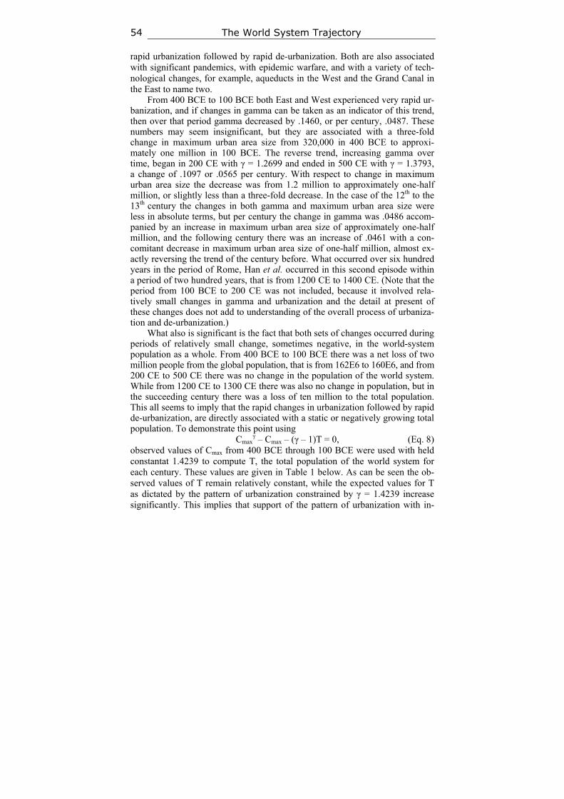
The World System Trajectory 54
rapid urbanization followed by rapid de-urbanization. Both are also associated with significant pandemics, with epidemic warfare, and with a variety of tech-nological changes, for example, aqueducts in the West and the Grand Canal in the East to name two.
From 400 BCE to 100 BCE both East and West experienced very rapid ur-banization, and if changes in gamma can be taken as an indicator of this trend, then over that period gamma decreased by .1460, or per century, .0487. These numbers may seem insignificant, but they are associated with a three-fold change in maximum urban area size from 320,000 in 400 BCE to approxi-mately one million in 100 BCE. The reverse trend, increasing gamma over time, began in 200 CE with γ = 1.2699 and ended in 500 CE with γ = 1.3793, a change of .1097 or .0565 per century. With respect to change in maximum urban area size the decrease was from 1.2 million to approximately one-half million, or slightly less than a three-fold decrease. In the case of the 12th to the 13th century the changes in both gamma and maximum urban area size were less in absolute terms, but per century the change in gamma was .0486 accom-panied by an increase in maximum urban area size of approximately one-half million, and the following century there was an increase of .0461 with a con-comitant decrease in maximum urban area size of one-half million, almost ex-actly reversing the trend of the century before. What occurred over six hundred years in the period of Rome, Han et al. occurred in this second episode within a period of two hundred years, that is from 1200 CE to 1400 CE. (Note that the period from 100 BCE to 200 CE was not included, because it involved rela-tively small changes in gamma and urbanization and the detail at present of these changes does not add to understanding of the overall process of urbaniza-tion and de-urbanization.)
What also is significant is the fact that both sets of changes occurred during periods of relatively small change, sometimes negative, in the world-system population as a whole. From 400 BCE to 100 BCE there was a net loss of two million people from the global population, that is from 162E6 to 160E6, and from 200 CE to 500 CE there was no change in the population of the world system. While from 1200 CE to 1300 CE there was also no change in population, but in the succeeding century there was a loss of ten million to the total population. This all seems to imply that the rapid changes in urbanization followed by rapid de-urbanization, are directly associated with a static or negatively growing total population. To demonstrate this point using
Cmaxγ – Cmax – (γ – 1)T = 0, (Eq. 8)
observed values of Cmax from 400 BCE through 100 BCE were used with held constantat 1.4239 to compute T, the total population of the world system for each century. These values are given in Table 1 below. As can be seen the ob-served values of T remain relatively constant, while the expected values for T as dictated by the pattern of urbanization constrained by γ = 1.4239 increase significantly. This implies that support of the pattern of urbanization with in-
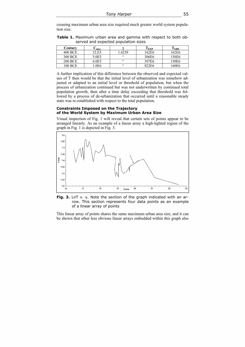
Tony Harper 55
creasing maximum urban area size required much greater world system popula-tion size.
Table 1. Maximum urban area and gamma with respect to both ob-served and expected population sizes
Century Cmax γ TEXP TOBS
400 BCE 32.E5 1.4239 162E6 162E6 300 BCE 5.0E5 “ 306E6 156E6 200 BCE 6.0E5 “ 397E6 150E6 100 BCE 1.0E6 “ 822E6 160E6
A further implication of this difference between the observed and expected val-ues of T then would be that the initial level of urbanization was somehow ad-justed or adapted to an initial level or threshold of population, but when the process of urbanization continued but was not underwritten by continued total population growth, then after a time delay exceeding that threshold was fol-lowed by a process of de-urbanization that occurred until a reasonable steady state was re-established with respect to the total population.
Constraints Imposed on the Trajectory of the World System by Maximum Urban Area Size
Visual inspection of Fig. 1 will reveal that certain sets of points appear to be arranged linearly. As an example of a linear array a high-lighted region of the graph in Fig. 1 is depicted in Fig. 3.
Fig. 3. LnT v. γ. Note the section of the graph indicated with an ar-
row. This section represents four data points as an example of a linear array of points
This linear array of points shares the same maximum urban area size, and it can be shown that other less obvious linear arrays embedded within this graph also
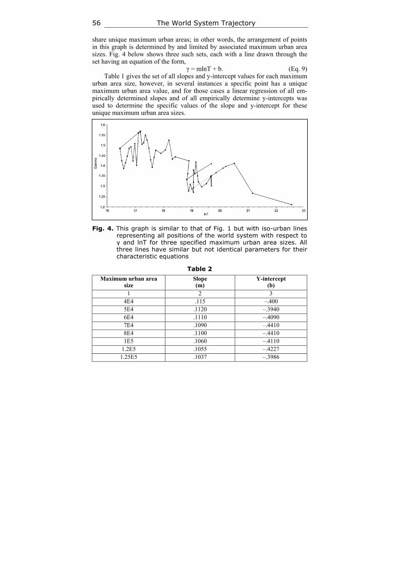
The World System Trajectory 56
share unique maximum urban areas; in other words, the arrangement of points in this graph is determined by and limited by associated maximum urban area sizes. Fig. 4 below shows three such sets, each with a line drawn through the set having an equation of the form,
γ = mlnT + b. (Eq. 9) Table 1 gives the set of all slopes and y-intercept values for each maximum
urban area size, however, in several instances a specific point has a unique maximum urban area value, and for those cases a linear regression of all em-pirically determined slopes and of all empirically determine y-intercepts was used to determine the specific values of the slope and y-intercept for these unique maximum urban area sizes.
Fig. 4. This graph is similar to that of Fig. 1 but with iso-urban lines
representing all positions of the world system with respect to γ and lnT for three specified maximum urban area sizes. All three lines have similar but not identical parameters for their characteristic equations
Table 2
Maximum urban area size
Slope (m)
Y-intercept (b)
1 2 3 4E4 .115 –.400 5E4 .1120 –.3940 6E4 .1110 –.4090 7E4 .1090 –.4410 8E4 .1100 –.4410 1E5 .1060 –.4110
1.2E5 .1055 –.4227 1.25E5 .1037 –.3986
Tony Harper 57
1 2 3 2E5 .1006 –.4104
3.2E5 .0980 –.4393 4E5 .0967 –.4440 5E5 .0948 –.4532 6E5 .0946 –.4532 7E5 .0938 –.4560 8E5 .0944 –.4801 9E5 .0927 –.4614 1E6 .0910 –.4430
1.1E6 .0918 –.4614 1.2E6 .0926 –.4946 1.5E6 .0906 –.4723 6.5E6 .0858 –.5037 35E6 .0828 –.5308
Note: Numbers in bold face type were produced by linear regression of empirically de-termined slopes and y-intercepts. All slope and intercept values can be substituted into an equation of the form, γ = mlnT + b.
There are several consequences of this finding. First, it is entirely possible to determine the position of an ordered pair of values of lnT and γ as the position of that point must lie on the appropriate linear array, here referred to as an iso-urban line, as determined by specific maximum urban area size. Second, the set of all linear arrays falls on a complex curved surface as determined by the range of values of both slope and y-intercept. Third, this surface must be undu-latory as slope and y-intercept values change with respect to maximum urban area size, while slope appears to decrease with respect to maximum urban area size, y-intercept values fluctuate, for example, the sequence from 4E4 through 2E5 exhibits continually decreasing slope values but decreasing then increasing then decreasing values of b. Fourth, the distance over which the world system moves is directly determined by maximum urban area. Fifth, since change in position of the world system from century to century can be represented by angular change with respect to a given iso-urban line and the actual distance moved, the world system trajectory can be represented by polar coordinates. This last aspect will investigated in the next section.
A Polar Plot Representation of the World System Trajectory
As was previously mentioned iso-urban lines can be used to generate a polar-plot of the world system trajectory. This was done in the following way. Local distance, defined as the distance from one point representing the position of the world system to a consecutive point was determined by the formula
d = [(γ1 – γ0 )2 + (lnT1 – lnT0)
2].5. (Eq. 10)
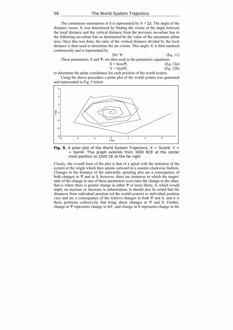
The World System Trajectory 58
The continuous summation of d is represented by S = Σd. The angle of the distance vector, θ, was determined by finding the cosine of the angle between the local distance and the vertical distance from the previous iso-urban line to the following iso-urban line as determined be the value of the maximum urban area. Once this was done, the ratio of the vertical distance divided by the local distance is then used to determine the arc cosine. This angle, θ, is then summed continuously and is represented by
Σθ= Ψ. (Eq. 11) These parameters, S and Ψ, are then used in the parametric equations:
X = ScosΨ, (Eq. 12a) Y = SsinΨ, (Eq. 12b)
to determine the polar coordinates for each position of the world system. Using the above procedure a polar plot of the world system was generated
and represented in Fig. 5 below.
Fig. 5. A polar plot of the World System Trajectory. X = ScosΨ. Y =
= SsinΨ. This graph extends from 3000 BCE at the center most position to 2000 CE at the far right
Clearly, the overall form of the plot is that of a spiral with the initiation of the system at the origin which then spirals outward in a counter-clockwise fashion. Changes in the distance of the outwardly spiraling plot are a consequence of both changes in Ψ and in S, however, there are instances in which the magni-tude of the change in one of these parameters over-rides the change in the other, that is where there is greater change in either Ψ or more likely, S, which would imply an increase or decrease in urbanization. It should also be noted that the distances from individual position (of the world-system) to individual position vary and are a consequence of the relative changes in both Ψ and S, and it is these positions collectively that bring about changes in Ψ and S. Further, change in Ψ represents change in lnT, and change in S represents change in the
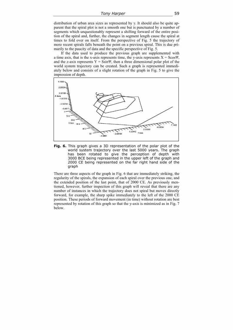
Tony Harper 59
distribution of urban area sizes as represented by γ. It should also be quite ap-parent that the spiral plot is not a smooth one but is punctuated by a number of segments which unquestionably represent a shifting forward of the entire posi-tion of the spiral and, further, the changes in segment length cause the spiral at times to fold over on itself. From the perspective of Fig. 5 the trajectory of more recent spirals falls beneath the point on a previous spiral. This is due pri-marily to the paucity of data and the specific perspective of Fig. 5.
If the data used to produce the previous graph are supplemented with a time axis, that is the x-axis represents time, the y-axis represents X = ScosΨ, and the z-axis represents Y = SsinΨ, then a three dimensional polar plot of the world system trajectory can be created. Such a graph is represented immedi-ately below and consists of a slight rotation of the graph in Fig. 5 to give the impression of depth.
Fig. 6. This graph gives a 3D representation of the polar plot of the world system trajectory over the last 5000 years. The graph has been rotated to give the perception of depth with 3000 BCE being represented in the upper left of the graph and 2000 CE being represented on the far right hand side of the graph
There are three aspects of the graph in Fig. 6 that are immediately striking, the regularity of the spirals, the expansion of each spiral over the previous one, and the extended position of the last point, that of 2000 CE. As previously men-tioned, however, further inspection of this graph will reveal that there are any number of instances in which the trajectory does not spiral but moves directly forward, for example, the sharp spike immediately to the left of the 2000 CE position. These periods of forward movement (in time) without rotation are best represented by rotation of this graph so that the y-axis is minimized as in Fig. 7 below.
Z Axis
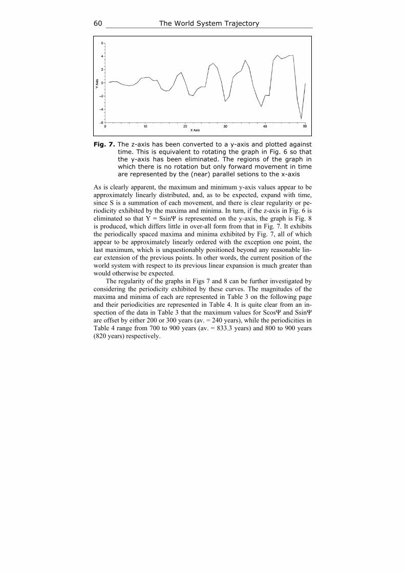
The World System Trajectory 60
Fig. 7. The z-axis has been converted to a y-axis and plotted against
time. This is equivalent to rotating the graph in Fig. 6 so that the y-axis has been eliminated. The regions of the graph in which there is no rotation but only forward movement in time are represented by the (near) parallel setions to the x-axis
As is clearly apparent, the maximum and minimum y-axis values appear to be approximately linearly distributed, and, as to be expected, expand with time, since S is a summation of each movement, and there is clear regularity or pe-riodicity exhibited by the maxima and minima. In turn, if the z-axis in Fig. 6 is eliminated so that Y = SsinΨ is represented on the y-axis, the graph is Fig. 8 is produced, which differs little in over-all form from that in Fig. 7. It exhibits the periodically spaced maxima and minima exhibited by Fig. 7, all of which appear to be approximately linearly ordered with the exception one point, the last maximum, which is unquestionably positioned beyond any reasonable lin-ear extension of the previous points. In other words, the current position of the world system with respect to its previous linear expansion is much greater than would otherwise be expected.
The regularity of the graphs in Figs 7 and 8 can be further investigated by considering the periodicity exhibited by these curves. The magnitudes of the maxima and minima of each are represented in Table 3 on the following page and their periodicities are represented in Table 4. It is quite clear from an in-spection of the data in Table 3 that the maximum values for ScosΨ and SsinΨ are offset by either 200 or 300 years (av. = 240 years), while the periodicities in Table 4 range from 700 to 900 years (av. = 833.3 years) and 800 to 900 years (820 years) respectively.
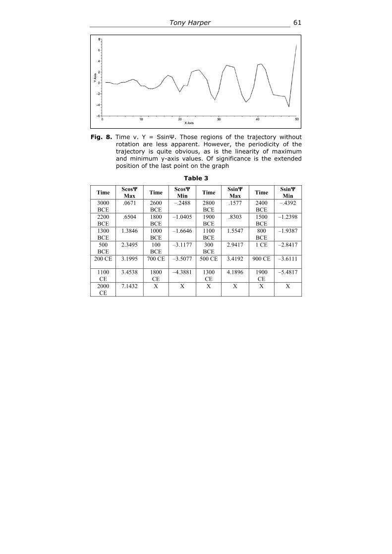
Tony Harper 61
Fig. 8. Time v. Y = SsinΨ. Those regions of the trajectory without
rotation are less apparent. However, the periodicity of the trajectory is quite obvious, as is the linearity of maximum and minimum y-axis values. Of significance is the extended position of the last point on the graph
Table 3
Time ScosΨ Max
Time ScosΨ Min
Time SsinΨ Max
Time SsinΨ Min
3000 BCE
.0671 2600 BCE
–.2488 2800 BCE
.1577 2400 BCE
–.4392
2200 BCE
.6504 1800 BCE
–1.0405 1900 BCE
.8303 1500 BCE
–1.2398
1300 BCE
1.3846 1000 BCE
–1.6646 1100 BCE
1.5547 800 BCE
–1.9387
500 BCE
2.3495 100 BCE
–3.1177 300 BCE
2.9417 1 CE –2.8417
200 CE 3.1995 700 CE –3.5077 500 CE 3.4192 900 CE –3.6111
1100 CE
3.4538 1800 CE
–4.3881 1300 CE
4.1896 1900 CE
–5.4817
2000 CE
7.1432 X X X X X X
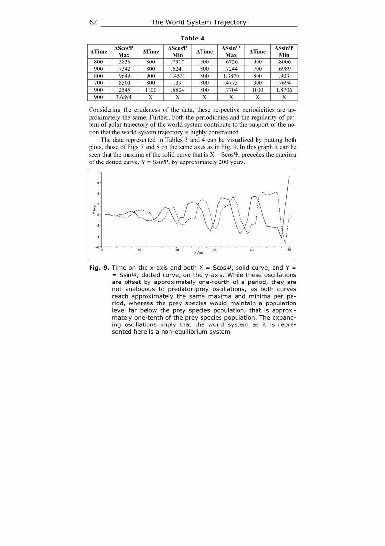
The World System Trajectory 62
Table 4
ΔTime ΔScosΨ
Max ΔTime
ΔScosΨ Min
ΔTime ΔSsinΨ
Max ΔTime
ΔSsinΨ Min
800 .5833 800 .7917 900 .6726 900 .8006 900 .7342 800 .6241 800 .7244 700 .6989 800 .9649 900 1.4531 800 1.3870 800 .903 700 .8500 800 .39 800 .4775 900 .7694 900 .2545 1100 .8804 800 .7704 1000 1.8706 900 3.6894 X X X X X X
Considering the crudeness of the data, these respective periodicities are ap-proximately the same. Further, both the periodicities and the regularity of pat-tern of polar trajectory of the world system contribute to the support of the no-tion that the world system trajectory is highly constrained.
The data represented in Tables 3 and 4 can be visualized by putting both plots, those of Figs 7 and 8 on the same axes as in Fig. 9. In this graph it can be seen that the maxima of the solid curve that is X = ScosΨ, precedes the maxima of the dotted curve, Y = SsinΨ, by approximately 200 years.
Fig. 9. Time on the x-axis and both X = ScosΨ, solid curve, and Y =
= SsinΨ, dotted curve, on the y-axis. While these oscillations are offset by approximately one-fourth of a period, they are not analogous to predator-prey oscillations, as both curves reach approximately the same maxima and minima per pe-riod, whereas the prey species would maintain a population level far below the prey species population, that is approxi-mately one-tenth of the prey species population. The expand-ing oscillations imply that the world system as it is repre-sented here is a non-equilibrium system
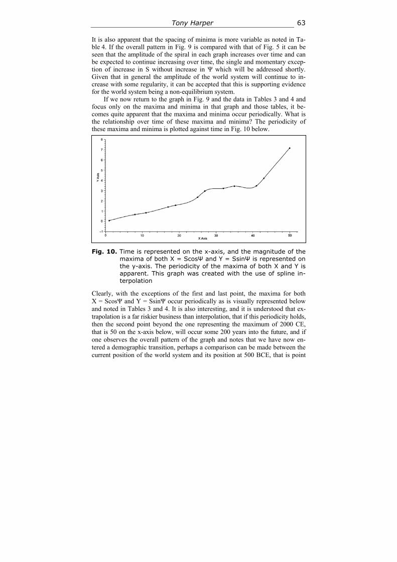
Tony Harper 63
It is also apparent that the spacing of minima is more variable as noted in Ta-ble 4. If the overall pattern in Fig. 9 is compared with that of Fig. 5 it can be seen that the amplitude of the spiral in each graph increases over time and can be expected to continue increasing over time, the single and momentary excep-tion of increase in S without increase in Ψ which will be addressed shortly. Given that in general the amplitude of the world system will continue to in-crease with some regularity, it can be accepted that this is supporting evidence for the world system being a non-equilibrium system.
If we now return to the graph in Fig. 9 and the data in Tables 3 and 4 and focus only on the maxima and minima in that graph and those tables, it be-comes quite apparent that the maxima and minima occur periodically. What is the relationship over time of these maxima and minima? The periodicity of these maxima and minima is plotted against time in Fig. 10 below.
Fig. 10. Time is represented on the x-axis, and the magnitude of the
maxima of both X = ScosΨ and Y = SsinΨ is represented on the y-axis. The periodicity of the maxima of both X and Y is apparent. This graph was created with the use of spline in-terpolation
Clearly, with the exceptions of the first and last point, the maxima for both X = ScosΨ and Y = SsinΨ occur periodically as is visually represented below and noted in Tables 3 and 4. It is also interesting, and it is understood that ex-trapolation is a far riskier business than interpolation, that if this periodicity holds, then the second point beyond the one representing the maximum of 2000 CE, that is 50 on the x-axis below, will occur some 200 years into the future, and if one observes the overall pattern of the graph and notes that we have now en-tered a demographic transition, perhaps a comparison can be made between the current position of the world system and its position at 500 BCE, that is point
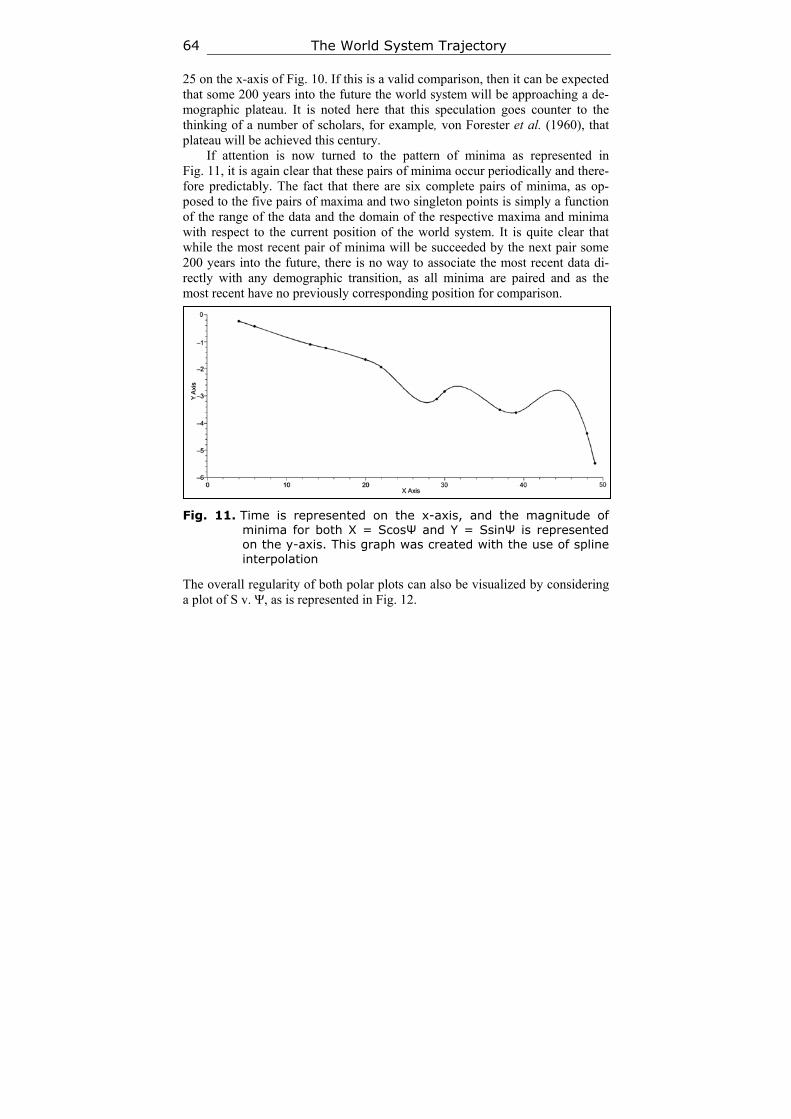
The World System Trajectory 64
25 on the x-axis of Fig. 10. If this is a valid comparison, then it can be expected that some 200 years into the future the world system will be approaching a de-mographic plateau. It is noted here that this speculation goes counter to the thinking of a number of scholars, for example, von Forester et al. (1960), that plateau will be achieved this century.
If attention is now turned to the pattern of minima as represented in Fig. 11, it is again clear that these pairs of minima occur periodically and there-fore predictably. The fact that there are six complete pairs of minima, as op-posed to the five pairs of maxima and two singleton points is simply a function of the range of the data and the domain of the respective maxima and minima with respect to the current position of the world system. It is quite clear that while the most recent pair of minima will be succeeded by the next pair some 200 years into the future, there is no way to associate the most recent data di-rectly with any demographic transition, as all minima are paired and as the most recent have no previously corresponding position for comparison.
Fig. 11. Time is represented on the x-axis, and the magnitude of
minima for both X = ScosΨ and Y = SsinΨ is represented on the y-axis. This graph was created with the use of spline interpolation
The overall regularity of both polar plots can also be visualized by considering a plot of S v. Ψ, as is represented in Fig. 12.
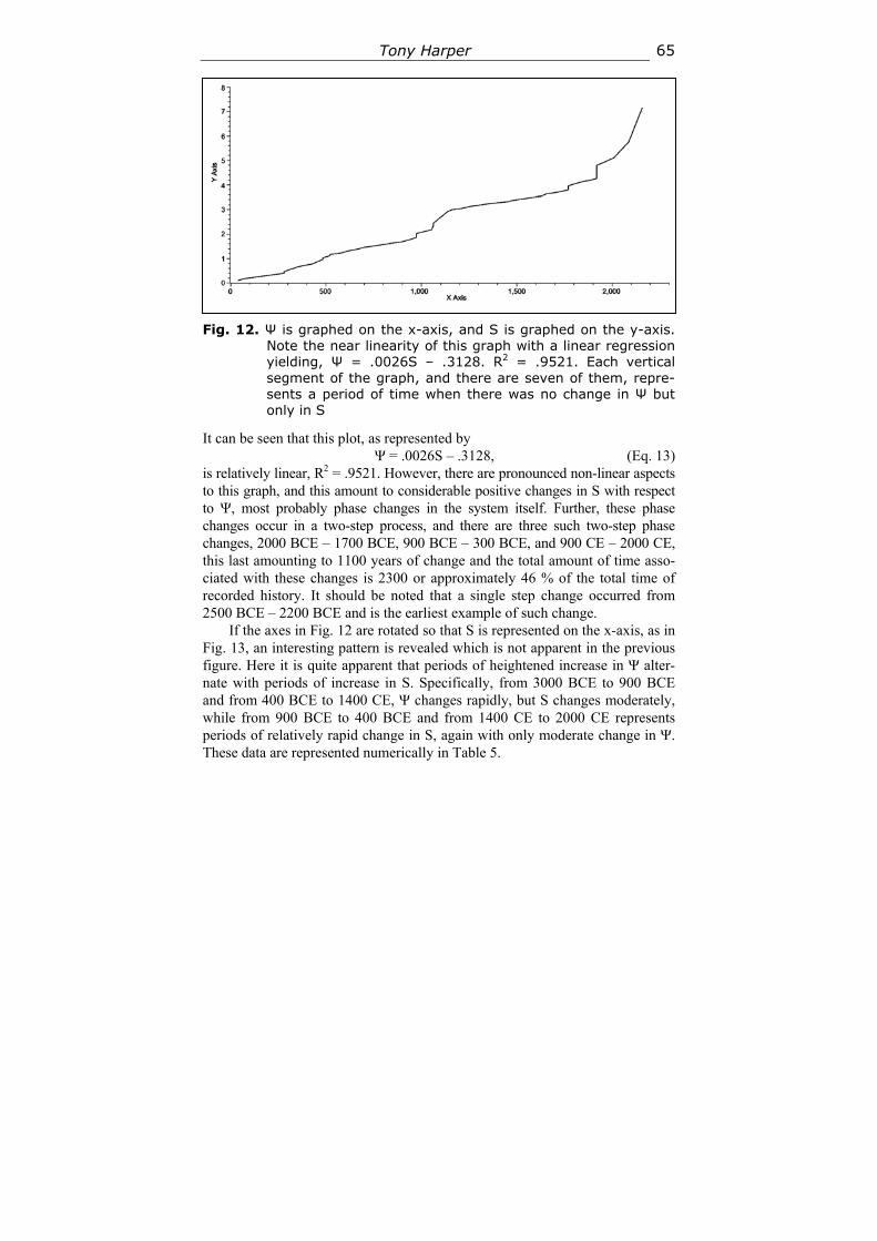
Tony Harper 65
Fig. 12. Ψ is graphed on the x-axis, and S is graphed on the y-axis.
Note the near linearity of this graph with a linear regression yielding, Ψ = .0026S – .3128. R2 = .9521. Each vertical segment of the graph, and there are seven of them, repre-sents a period of time when there was no change in Ψ but only in S
It can be seen that this plot, as represented by Ψ = .0026S – .3128, (Eq. 13)
is relatively linear, R2 = .9521. However, there are pronounced non-linear aspects to this graph, and this amount to considerable positive changes in S with respect to Ψ, most probably phase changes in the system itself. Further, these phase changes occur in a two-step process, and there are three such two-step phase changes, 2000 BCE – 1700 BCE, 900 BCE – 300 BCE, and 900 CE – 2000 CE, this last amounting to 1100 years of change and the total amount of time asso-ciated with these changes is 2300 or approximately 46 % of the total time of recorded history. It should be noted that a single step change occurred from 2500 BCE – 2200 BCE and is the earliest example of such change.
If the axes in Fig. 12 are rotated so that S is represented on the x-axis, as in Fig. 13, an interesting pattern is revealed which is not apparent in the previous figure. Here it is quite apparent that periods of heightened increase in Ψ alter-nate with periods of increase in S. Specifically, from 3000 BCE to 900 BCE and from 400 BCE to 1400 CE, Ψ changes rapidly, but S changes moderately, while from 900 BCE to 400 BCE and from 1400 CE to 2000 CE represents periods of relatively rapid change in S, again with only moderate change in Ψ. These data are represented numerically in Table 5.
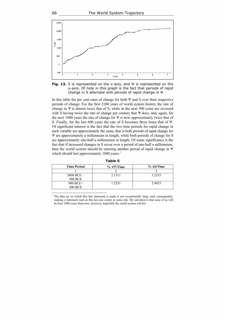
The World System Trajectory 66
Fig. 13. S is represented on the x-axis, and Ψ is represented on the y-axis. Of note in this graph is the fact that periods of rapid change in S alternate with periods of rapid change in Ψ
In this table the per cent rates of change for both Ψ and S over their respective periods of change. For the first 2100 years of world system history the rate of change in Ψ is almost twice that of S, while in the next 500 years are reversed with S having twice the rate of change per century that Ψ does, and, again, for the next 1000 years the rate of change for Ψ is now approximately twice that of S. Finally, for the last 600 years the rate of S becomes three times that of Ψ. Of significant interest is the fact that the two time periods for rapid change in each variable are approximately the same, that is both periods of rapid change for Ψ are approximately a millennium in length, while both periods of change for S are approximately one-half a millennium in length. Of some significance is the fact that if increased changes in S occur over a period of one-half a millennium, then the world system should be entering another period of rapid change in Ψ which should last approximately 1000 years.1
Table 5
Time Period % ΔΨ/Time % ΔS/Time 1 2 3
3000 BCE – 900 BCE
2.1511 1.2335
900 BCE– 400 BCE
1.5251 2.9833
1 The data set on which this last statement is made is not exceptionally large, and, consequently,
making a statement such as this last one comes at some risk. My salvation is that none of us will be here 1000 years from now, however, hopefully the world system will be!
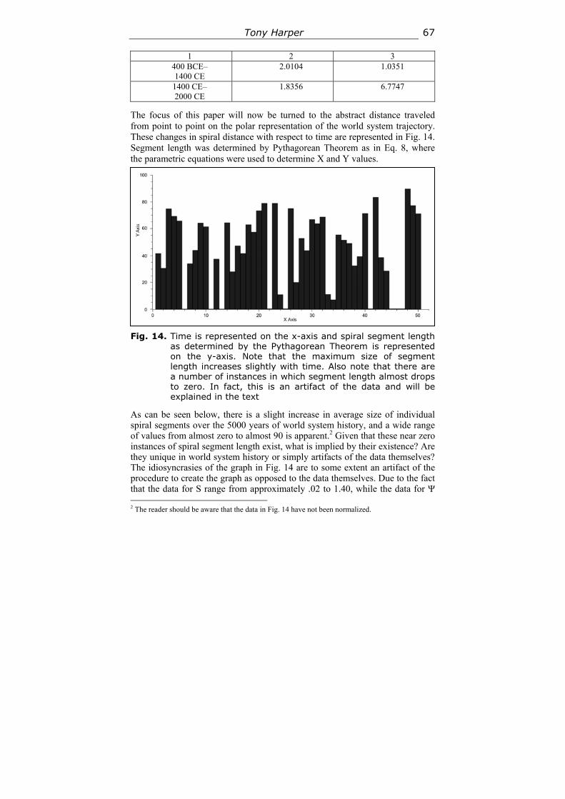
Tony Harper 67
1 2 3 400 BCE– 1400 CE
2.0104 1.0351
1400 CE– 2000 CE
1.8356 6.7747
The focus of this paper will now be turned to the abstract distance traveled from point to point on the polar representation of the world system trajectory. These changes in spiral distance with respect to time are represented in Fig. 14. Segment length was determined by Pythagorean Theorem as in Eq. 8, where the parametric equations were used to determine X and Y values.
Fig. 14. Time is represented on the x-axis and spiral segment length
as determined by the Pythagorean Theorem is represented on the y-axis. Note that the maximum size of segment length increases slightly with time. Also note that there are a number of instances in which segment length almost drops to zero. In fact, this is an artifact of the data and will be explained in the text
As can be seen below, there is a slight increase in average size of individual spiral segments over the 5000 years of world system history, and a wide range of values from almost zero to almost 90 is apparent.2 Given that these near zero instances of spiral segment length exist, what is implied by their existence? Are they unique in world system history or simply artifacts of the data themselves? The idiosyncrasies of the graph in Fig. 14 are to some extent an artifact of the procedure to create the graph as opposed to the data themselves. Due to the fact that the data for S range from approximately .02 to 1.40, while the data for Ψ 2 The reader should be aware that the data in Fig. 14 have not been normalized.
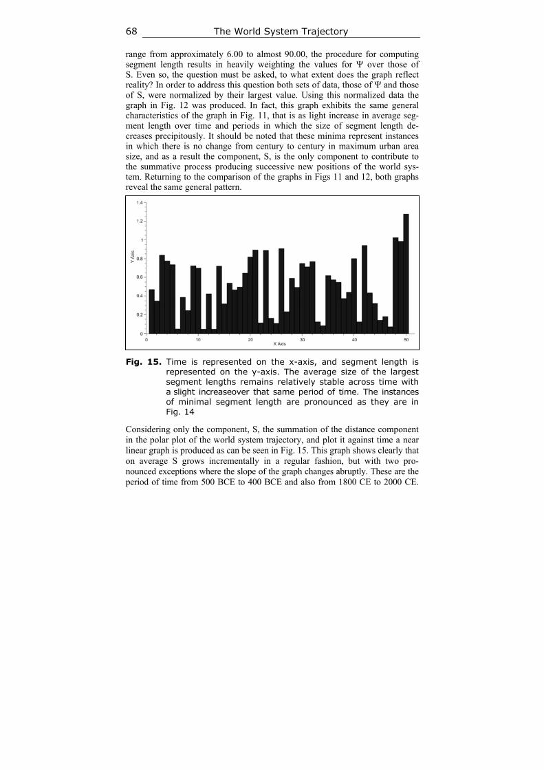
The World System Trajectory 68
range from approximately 6.00 to almost 90.00, the procedure for computing segment length results in heavily weighting the values for Ψ over those of S. Even so, the question must be asked, to what extent does the graph reflect reality? In order to address this question both sets of data, those of Ψ and those of S, were normalized by their largest value. Using this normalized data the graph in Fig. 12 was produced. In fact, this graph exhibits the same general characteristics of the graph in Fig. 11, that is as light increase in average seg-ment length over time and periods in which the size of segment length de-creases precipitously. It should be noted that these minima represent instances in which there is no change from century to century in maximum urban area size, and as a result the component, S, is the only component to contribute to the summative process producing successive new positions of the world sys-tem. Returning to the comparison of the graphs in Figs 11 and 12, both graphs reveal the same general pattern.
Fig. 15. Time is represented on the x-axis, and segment length is represented on the y-axis. The average size of the largest segment lengths remains relatively stable across time with a slight increaseover that same period of time. The instances of minimal segment length are pronounced as they are in Fig. 14
Considering only the component, S, the summation of the distance component in the polar plot of the world system trajectory, and plot it against time a near linear graph is produced as can be seen in Fig. 15. This graph shows clearly that on average S grows incrementally in a regular fashion, but with two pro-nounced exceptions where the slope of the graph changes abruptly. These are the period of time from 500 BCE to 400 BCE and also from 1800 CE to 2000 CE.
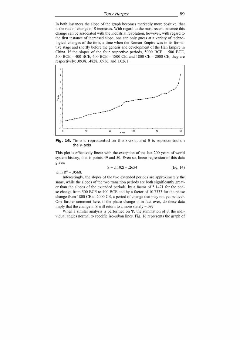
Tony Harper 69
In both instances the slope of the graph becomes markedly more positive, that is the rate of change of S increases. With regard to the most recent instance this change can be associated with the industrial revolution, however, with regard to the first instance of increased slope, one can only guess at a variety of techno-logical changes of the time, a time when the Roman Empire was in its forma-tive stage and shortly before the genesis and development of the Han Empire in China. If the slopes of the four respective periods, 5000 BCE – 500 BCE, 500 BCE – 400 BCE, 400 BCE – 1800 CE, and 1800 CE – 2000 CE, they are respectively: .0938, .4828, .0956, and 1.0261.
Fig. 16. Time is represented on the x-axis, and S is represented on the y-axis
This plot is effectively linear with the exception of the last 200 years of world system history, that is points 49 and 50. Even so, linear regression of this data gives:
S = .1102t – .2654 (Eq. 14) with R2 = .9568.
Interestingly, the slopes of the two extended periods are approximately the same, while the slopes of the two transition periods are both significantly great-er than the slopes of the extended periods, by a factor of 5.1471 for the pha- se change from 500 BCE to 400 BCE and by a factor of 10.7333 for the phase change from 1800 CE to 2000 CE, a period of change that may not yet be over. One further comment here, if the phase change is in fact over, do these data imply that the change in S will return to a more stately ~.09?
When a similar analysis is performed on Ψ, the summation of θ, the indi-vidual angles normal to specific iso-urban lines. Fig. 16 represents the graph of
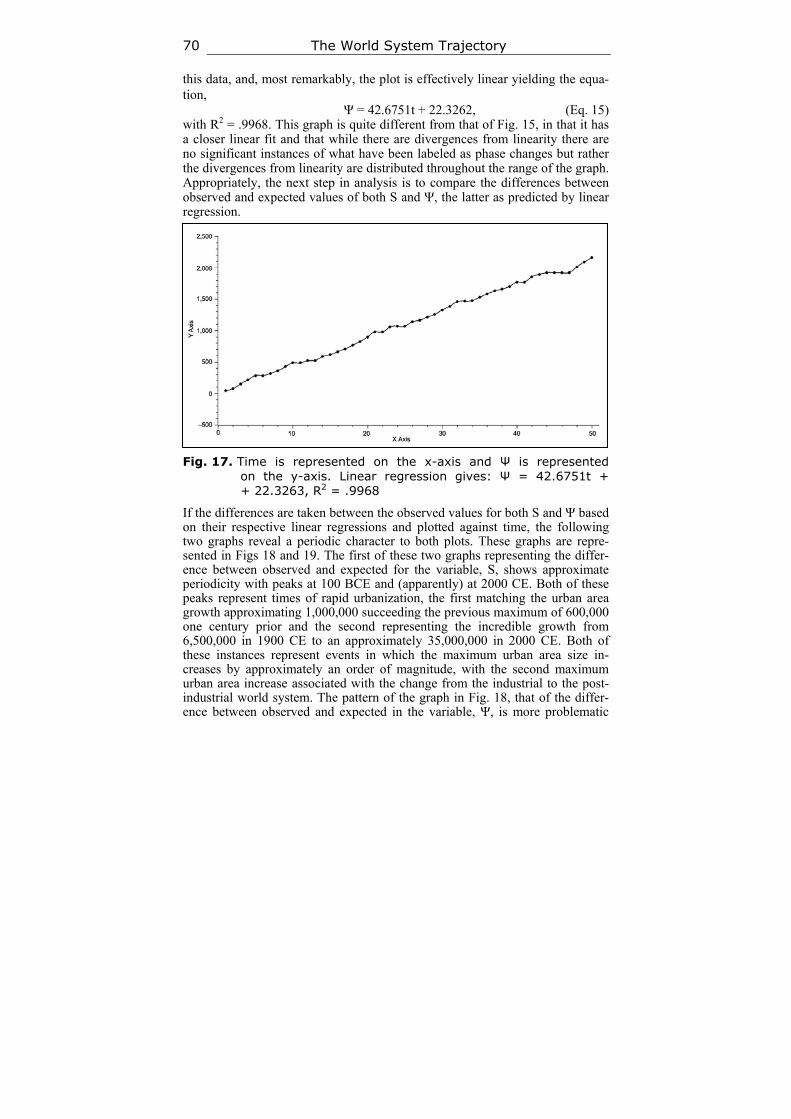
The World System Trajectory 70
this data, and, most remarkably, the plot is effectively linear yielding the equa-tion,
Ψ = 42.6751t + 22.3262, (Eq. 15) with R2 = .9968. This graph is quite different from that of Fig. 15, in that it has a closer linear fit and that while there are divergences from linearity there are no significant instances of what have been labeled as phase changes but rather the divergences from linearity are distributed throughout the range of the graph. Appropriately, the next step in analysis is to compare the differences between observed and expected values of both S and Ψ, the latter as predicted by linear regression.
Fig. 17. Time is represented on the x-axis and Ψ is represented
on the y-axis. Linear regression gives: Ψ = 42.6751t + + 22.3263, R2 = .9968
If the differences are taken between the observed values for both S and Ψ based on their respective linear regressions and plotted against time, the following two graphs reveal a periodic character to both plots. These graphs are repre-sented in Figs 18 and 19. The first of these two graphs representing the differ-ence between observed and expected for the variable, S, shows approximate periodicity with peaks at 100 BCE and (apparently) at 2000 CE. Both of these peaks represent times of rapid urbanization, the first matching the urban area growth approximating 1,000,000 succeeding the previous maximum of 600,000 one century prior and the second representing the incredible growth from 6,500,000 in 1900 CE to an approximately 35,000,000 in 2000 CE. Both of these instances represent events in which the maximum urban area size in-creases by approximately an order of magnitude, with the second maximum urban area increase associated with the change from the industrial to the post-industrial world system. The pattern of the graph in Fig. 18, that of the differ-ence between observed and expected in the variable, Ψ, is more problematic
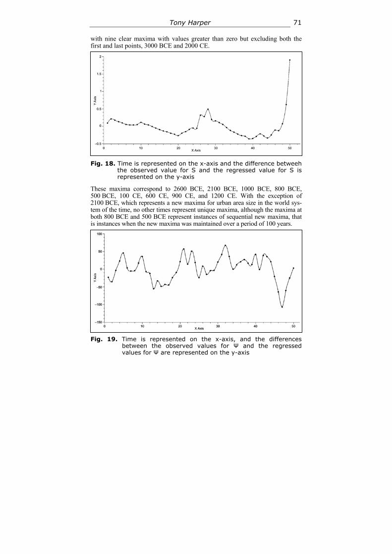
Tony Harper 71
with nine clear maxima with values greater than zero but excluding both the first and last points, 3000 BCE and 2000 CE.
Fig. 18. Time is represented on the x-axis and the difference betweeh the observed value for S and the regressed value for S is represented on the y-axis
These maxima correspond to 2600 BCE, 2100 BCE, 1000 BCE, 800 BCE, 500 BCE, 100 CE, 600 CE, 900 CE, and 1200 CE. With the exception of 2100 BCE, which represents a new maxima for urban area size in the world sys-tem of the time, no other times represent unique maxima, although the maxima at both 800 BCE and 500 BCE represent instances of sequential new maxima, that is instances when the new maxima was maintained over a period of 100 years.
Fig. 19. Time is represented on the x-axis, and the differences
between the observed values for Ψ and the regressed values for Ψ are represented on the y-axis
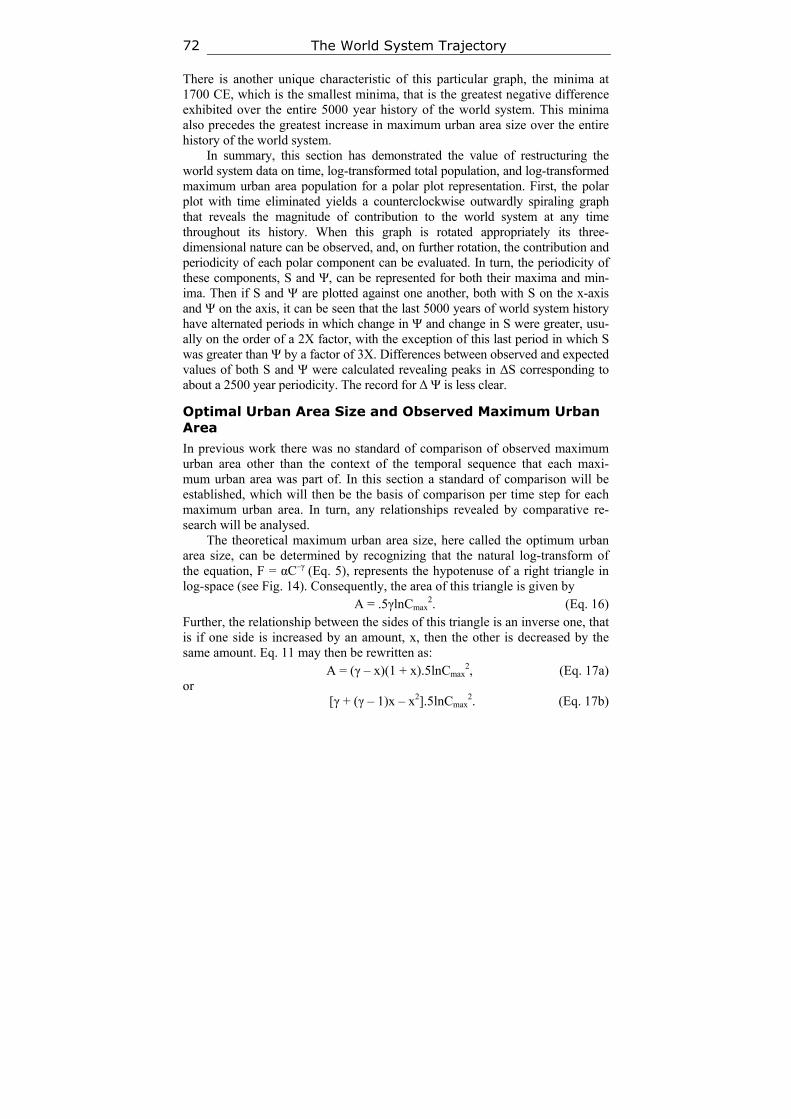
The World System Trajectory 72
There is another unique characteristic of this particular graph, the minima at 1700 CE, which is the smallest minima, that is the greatest negative difference exhibited over the entire 5000 year history of the world system. This minima also precedes the greatest increase in maximum urban area size over the entire history of the world system.
In summary, this section has demonstrated the value of restructuring the world system data on time, log-transformed total population, and log-transformed maximum urban area population for a polar plot representation. First, the polar plot with time eliminated yields a counterclockwise outwardly spiraling graph that reveals the magnitude of contribution to the world system at any time throughout its history. When this graph is rotated appropriately its three-dimensional nature can be observed, and, on further rotation, the contribution and periodicity of each polar component can be evaluated. In turn, the periodicity of these components, S and Ψ, can be represented for both their maxima and min-ima. Then if S and Ψ are plotted against one another, both with S on the x-axis and Ψ on the axis, it can be seen that the last 5000 years of world system history have alternated periods in which change in Ψ and change in S were greater, usu-ally on the order of a 2X factor, with the exception of this last period in which S was greater than Ψ by a factor of 3X. Differences between observed and expected values of both S and Ψ were calculated revealing peaks in ΔS corresponding to about a 2500 year periodicity. The record for Δ Ψ is less clear.
Optimal Urban Area Size аnd Observed Maximum Urban Area
In previous work there was no standard of comparison of observed maximum urban area other than the context of the temporal sequence that each maxi- mum urban area was part of. In this section a standard of comparison will be established, which will then be the basis of comparison per time step for each maximum urban area. In turn, any relationships revealed by comparative re-search will be analysed.
The theoretical maximum urban area size, here called the optimum urban area size, can be determined by recognizing that the natural log-transform of the equation, F = αC–γ (Eq. 5), represents the hypotenuse of a right triangle in log-space (see Fig. 14). Consequently, the area of this triangle is given by
A = .5γlnCmax2. (Eq. 16)
Further, the relationship between the sides of this triangle is an inverse one, that is if one side is increased by an amount, x, then the other is decreased by the same amount. Eq. 11 may then be rewritten as:
A = (γ – x)(1 + x).5lnCmax2, (Eq. 17a)
or [γ + (γ – 1)x – x2].5lnCmax
2. (Eq. 17b)
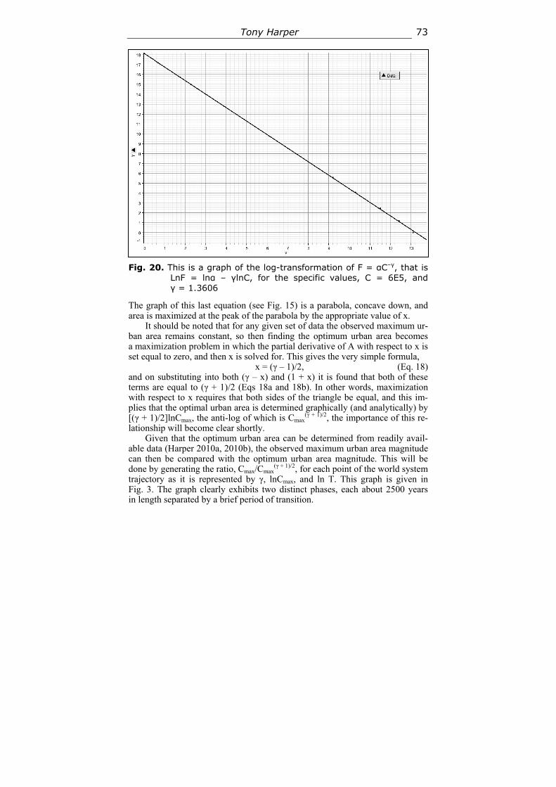
Tony Harper 73
Fig. 20. This is a graph of the log-transformation of F = αC–γ, that is
LnF = lnα – γlnC, for the specific values, C = 6E5, and γ = 1.3606
The graph of this last equation (see Fig. 15) is a parabola, concave down, and area is maximized at the peak of the parabola by the appropriate value of x.
It should be noted that for any given set of data the observed maximum ur-ban area remains constant, so then finding the optimum urban area becomes a maximization problem in which the partial derivative of A with respect to x is set equal to zero, and then x is solved for. This gives the very simple formula,
x = (γ – 1)/2, (Eq. 18) and on substituting into both (γ – x) and (1 + x) it is found that both of these terms are equal to (γ + 1)/2 (Eqs 18a and 18b). In other words, maximization with respect to x requires that both sides of the triangle be equal, and this im-plies that the optimal urban area is determined graphically (and analytically) by [(γ + 1)/2]lnCmax, the anti-log of which is Cmax
(γ + 1)/2, the importance of this re-lationship will become clear shortly.
Given that the optimum urban area can be determined from readily avail-able data (Harper 2010a, 2010b), the observed maximum urban area magnitude can then be compared with the optimum urban area magnitude. This will be done by generating the ratio, Cmax/Cmax
(γ + 1)/2, for each point of the world system trajectory as it is represented by γ, lnCmax, and ln T. This graph is given in Fig. 3. The graph clearly exhibits two distinct phases, each about 2500 years in length separated by a brief period of transition.
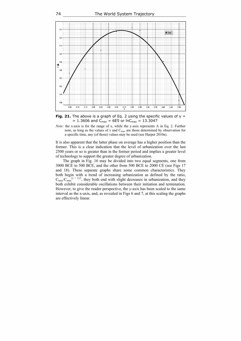
The World System Trajectory 74
Fig. 21. The above is a graph of Eq. 2 using the specific values of γ = = 1.3606 and Cmax = 6E5 or lnCmax = 13.3047
Note: the x-axis is for the range of x, while the y-axis represents A in Eq. 2. Further note, as long as the values of γ and Cmax are those determined by observation for a specific time, any (of those) values may be used (see Harper 2010a).
It is also apparent that the latter phase on average has a higher position than the former. This is a clear indication that the level of urbanization over the last 2500 years or so is greater than in the former period and implies a greater level of technology to support the greater degree of urbanization.
The graph in Fig. 16 may be divided into two equal segments, one from 3000 BCE to 500 BCE, and the other from 500 BCE to 2000 CE (see Figs 17 and 18). These separate graphs share some common characteristics. They both begin with a trend of increasing urbanization as defined by the ratio, Cmax/Cmax
(γ + 1)/2, they both end with slight decreases in urbanization, and they both exhibit considerable oscillations between their initiation and termination. However, to give the reader perspective, the y-axis has been scaled to the same interval as the x-axis, and, as revealed in Figs 6 and 7, at this scaling the graphs are effectively linear.
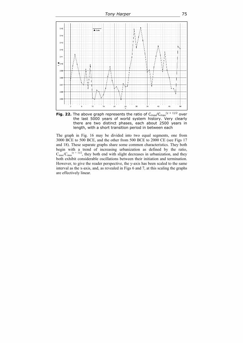
Tony Harper 75
Fig. 22. The above graph represents the ratio of Cmax/Cmax
(γ + 1)/2 over the last 5000 years of world system history. Very clearly there are two distinct phases, each about 2500 years in length, with a short transition period in between each
The graph in Fig. 16 may be divided into two equal segments, one from 3000 BCE to 500 BCE, and the other from 500 BCE to 2000 CE (see Figs 17 and 18). These separate graphs share some common characteristics. They both begin with a trend of increasing urbanization as defined by the ratio, Cmax/Cmax
(γ + 1)/2, they both end with slight decreases in urbanization, and they both exhibit considerable oscillations between their initiation and termination. However, to give the reader perspective, the y-axis has been scaled to the same interval as the x-axis, and, as revealed in Figs 6 and 7, at this scaling the graphs are effectively linear.
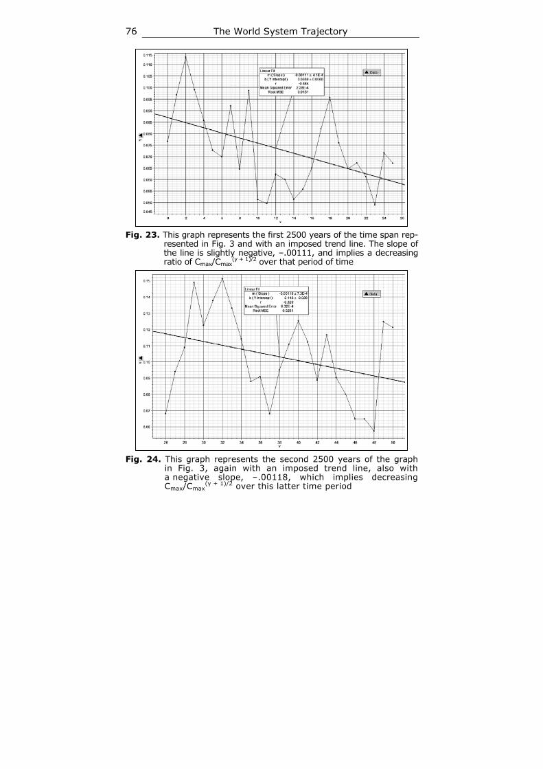
The World System Trajectory 76
Fig. 23. This graph represents the first 2500 years of the time span rep-
resented in Fig. 3 and with an imposed trend line. The slope of the line is slightly negative, –.00111, and implies a decreasing ratio of Cmax/Cmax
(γ + 1)/2 over that period of time
Fig. 24. This graph represents the second 2500 years of the graph
in Fig. 3, again with an imposed trend line, also with a negative slope, –.00118, which implies decreasing Cmax/Cmax
(γ + 1)/2 over this latter time period
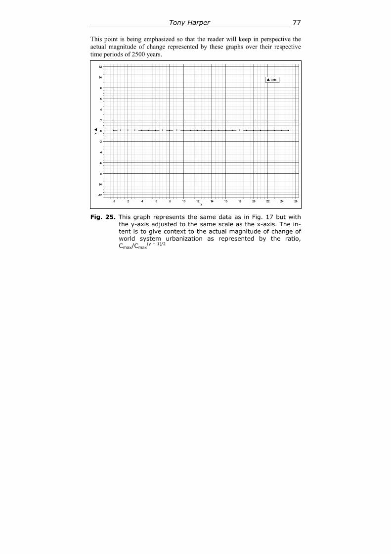
Tony Harper 77
This point is being emphasized so that the reader will keep in perspective the actual magnitude of change represented by these graphs over their respective time periods of 2500 years.
Fig. 25. This graph represents the same data as in Fig. 17 but with the y-axis adjusted to the same scale as the x-axis. The in-tent is to give context to the actual magnitude of change of world system urbanization as represented by the ratio, Cmax/Cmax
(γ + 1)/2

The World System Trajectory 78
Fig. 26. This graph is of the data represented in Fig. 18 but adjusted so
that both the x and y-axes are scaled the same as in Fig. 19
If linear regression is applied to both sets of data, that is data from both the first and second 2500 year periods, the respective linear equations,
CR = .0869 – .00111t, (Eq. 19) and
CR = .148 – .00118t, (Eq. 20), where CR represents the ratio, Cmax/Cmax
(γ + 1)/2, and t is time. The slopes of these regression equations are effectively the same, differing by only .00008, implying similar rates of average change with respect to the changing magnitude of Cmax/Cmax
(γ + 1)/2 over the two respective 2500 year periods. This can be more emphatically demonstrated by looking at a composite graph in Fig. 27 of both regression lines. In this graph the lower solid line represents the average change in the ratio, Cmax/Cmax
(γ + 1)/2, for the first 2500 years of world system history, and the higher solid line represents the same for the second 2500 years of world system history. Both lines have been extrapolated by a dashed line to represent the full extent of the trend had the trend been extended over the full 5000 years.
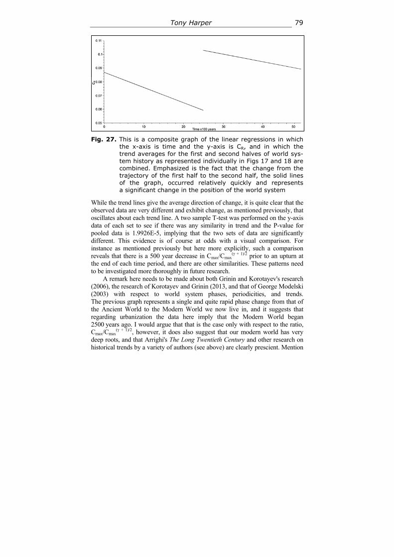
Tony Harper 79
Fig. 27. This is a composite graph of the linear regressions in which the x-axis is time and the y-axis is CR, and in which the trend averages for the first and second halves of world sys-tem history as represented individually in Figs 17 and 18 are combined. Emphasized is the fact that the change from the trajectory of the first half to the second half, the solid lines of the graph, occurred relatively quickly and represents a significant change in the position of the world system
While the trend lines give the average direction of change, it is quite clear that the observed data are very different and exhibit change, as mentioned previously, that oscillates about each trend line. A two sample T-test was performed on the y-axis data of each set to see if there was any similarity in trend and the P-value for pooled data is 1.9926E-5, implying that the two sets of data are significantly different. This evidence is of course at odds with a visual comparison. For instance as mentioned previously but here more explicitly, such a comparison reveals that there is a 500 year decrease in Cmax/Cmax
(γ + 1)/2 prior to an upturn at the end of each time period, and there are other similarities. These patterns need to be investigated more thoroughly in future research.
A remark here needs to be made about both Grinin and Korotayev's research (2006), the research of Korotayev and Grinin (2013, and that of George Modelski (2003) with respect to world system phases, periodicities, and trends. The previous graph represents a single and quite rapid phase change from that of the Ancient World to the Modern World we now live in, and it suggests that regarding urbanization the data here imply that the Modern World began 2500 years ago. I would argue that that is the case only with respect to the ratio, Cmax/Cmax
(γ + 1)/2, however, it does also suggest that our modern world has very deep roots, and that Arrighi's The Long Twentieth Century and other research on historical trends by a variety of authors (see above) are clearly prescient. Mention
CR
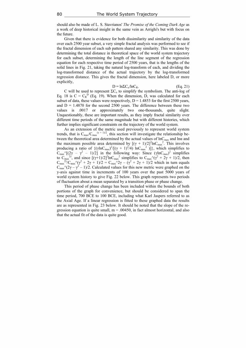
The World System Trajectory 80
should also be made of L. S. Stavrianos' The Promise of the Coming Dark Age as a work of deep historical insight in the same vein as Arrighi's but with focus on the future.
Given that there is evidence for both dissimilarity and similarity of the data over each 2500 year subset, a very simple fractal analysis was performed to see if the fractal dimension of each sub pattern shared any similarity. This was done by determining the total distance in theoretical space of the world system trajectory for each subset, determining the length of the line segment of the regression equation for each respective time period of 2500 years, that is the lengths of the solid lines in Fig. 21, taking the natural log-transform of each, and dividing the log-transformed distance of the actual trajectory by the log-transformed regression distance. This gives the fractal dimension, here labeled D, or more explicitly,
D = lnΣCo/lnCR. (Eq. 21) C will be used to represent ΣCo to simplify the symbolism. The anti-log of
Eq. 18 is C = CRD (Eq. 19). When the dimension, D, was calculated for each
subset of data, these values were respectively, D = 1.4853 for the first 2500 years, and D = 1.4870 for the second 2500 years. The difference between these two values is .0017 or approximately two one-thousands, quite slight. Unquestionably, these are important results, as they imply fractal similarity over different time periods of the same magnitude but with different histories, which further implies significant constraints on the trajectory of the world system.
As an extension of the metric used previously to represent world system trends, that is Cmax/Cmax
(γ + 1)/2, this section will investigate the relationship be-tween the theoretical area determined by the actual values of lnCmax and lnα and the maximum possible area determined by [(γ + 1)/2]2lnCmax
2. This involves producing a ratio of {(γlnCmax)
2/[(γ + 1)2/4) lnCmax2 )]}, which simplifies to
Cmax^[(2γ – γ2 – 1)/2] in the following way: Since (γlnCmax)2 simplifies
to Cmax2γ, and since [(γ+1)/2]2lnCmax
2 simplifies to Cmax^(γ2 + 2γ + 1)/2, then Cmax
2γ/Cmax^(γ2 + 2γ + 1)/2 = Cmax^2γ – (γ2 + 2γ + 1)/2 which in turn equals Cmax^(2γ – γ2 – 1)/2. Calculated values for this new metric were graphed on the y-axis against time in increments of 100 years over the past 5000 years of world system history to give Fig. 22 below. This graph represents two periods of fluctuation about a mean separated by a transition phase or phase change.
This period of phase change has been included within the bounds of both portions of the graph for convenience, but should be considered to span the time period, 700 BCE to 100 BCE, including what Karl Jaspers referred to as the Axial Age. If a linear regression is fitted to these graphed data the results are as represented in Fig. 23 below. It should be noted that the slope of the re-gression equation is quite small, m = .00450, in fact almost horizontal, and also that the actual fit of the data is quite good.
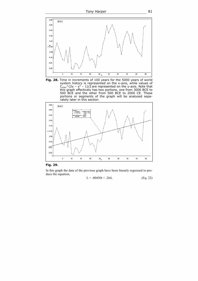
Tony Harper 81
Fig. 28. Time in increments of 100 years for the 5000 years of world
system history is represented on the x-axis, while values of Cmax^(2γ – γ2 – 1)/2are represented on the y-axis. Note that this graph effectively has two portions, one from 3000 BCE to 500 BCE and the other from 500 BCE to 2000 CE. These portions or segments of the graph will be analysed sepa-rately later in this section
Fig. 29.
In this graph the data of the previous graph have been linearly regressed to pro-duce the equation,
L = .00450t + .264, (Eq. 22)
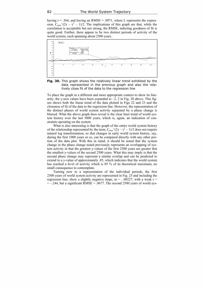
The World System Trajectory 82
having r = .564, and having an RMSE = .0971, where L represents the expres-sion, Cmax^(2γ – γ2 – 1)/2. The implications of this graph are that, while the correlation is acceptable but not strong, the RMSE, indicting goodness of fit is quite good. Further, there appear to be two distinct periods of activity of the world system, each spanning about 2500 years.
Fig. 30. This graph shows the relatively linear trend exhibited by the
data represented in the previous graph and also the rela-tively close fit of the data to the regression line
To place the graph in a different and more appropriate context to show its line-arity, the y-axis values have been expanded to –2, 2 in Fig. 30 above. This fig-ure shows both the linear trend of the data plotted in Figs 22 and 23 and the closeness of fit of the data to the regression line. However, the representation of the distinct phases of world system activity separated by a phase change is blurred. What the above graph does reveal is the clear liner trend of world sys-tem history over the last 5000 years, which is, again, an indication of con-straints operating on the system.
What is also interesting is that the graph of the entire world system history of the relationship represented by the term, Cmax^(2γ – γ2 – 1)/2 does not require natural log transformation, so that changes in early world system history, say, during the first 1000 years or so, can be compared directly with any other por-tion of the data plot. With this in mind, it should be noted that the system change in the phase change noted previously represents an overlapping of sys-tem activity in that the greatest y-values of the first 2500 years are greater that the smallest y-values of the second 2500 years. What this may imply is that the second phase change may represent a similar overlap and can be predicted to extend to a y-value of approximately .85, which indicates that the world system has reached a level of activity which is 85 % of its theoretical maximum, no small consequence to contemplate.
Turning now to a representation of the individual periods, the first 2500 years of world system activity are represented in Fig. 25 and including the regression line, show a slightly negative slope, m = –.00227, with a weak r = = –.244, but a significant RMSE = .0677. The second 2500 years of world sys-
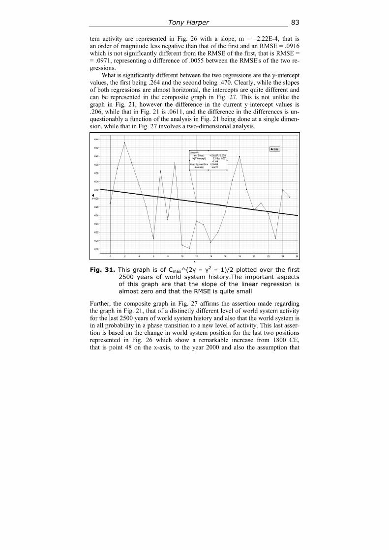
Tony Harper 83
tem activity are represented in Fig. 26 with a slope, m = –2.22E-4, that is an order of magnitude less negative than that of the first and an RMSE = .0916 which is not significantly different from the RMSE of the first, that is RMSE = = .0971, representing a difference of .0055 between the RMSE's of the two re-gressions.
What is significantly different between the two regressions are the y-intercept values, the first being .264 and the second being .470. Clearly, while the slopes of both regressions are almost horizontal, the intercepts are quite different and can be represented in the composite graph in Fig. 27. This is not unlike the graph in Fig. 21, however the difference in the current y-intercept values is .206, while that in Fig. 21 is .0611, and the difference in the differences is un-questionably a function of the analysis in Fig. 21 being done at a single dimen-sion, while that in Fig. 27 involves a two-dimensional analysis.
Х
Fig. 31. This graph is of Cmax^(2γ – γ2 – 1)/2 plotted over the first 2500 years of world system history.The important aspects of this graph are that the slope of the linear regression is almost zero and that the RMSE is quite small
Further, the composite graph in Fig. 27 affirms the assertion made regarding the graph in Fig. 21, that of a distinctly different level of world system activity for the last 2500 years of world system history and also that the world system is in all probability in a phase transition to a new level of activity. This last asser-tion is based on the change in world system position for the last two positions represented in Fig. 26 which show a remarkable increase from 1800 CE, that is point 48 on the x-axis, to the year 2000 and also the assumption that
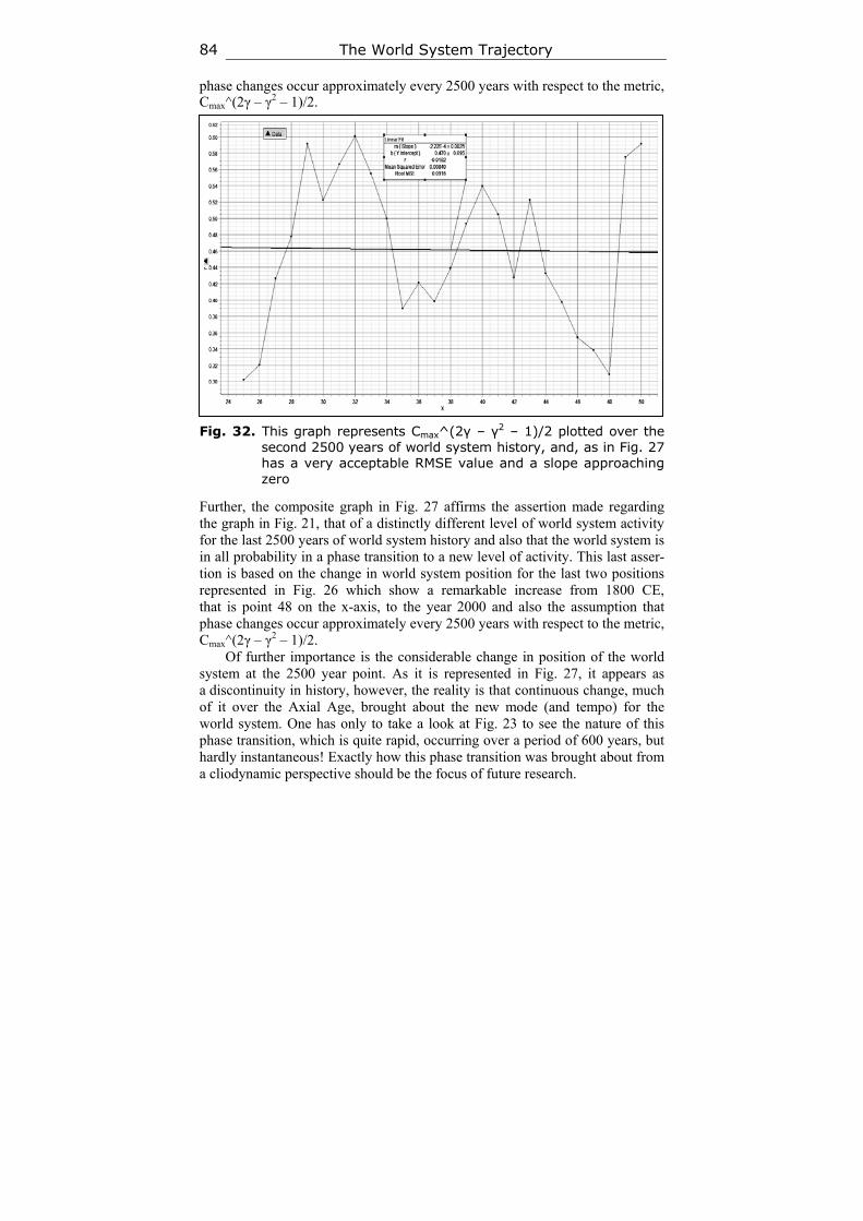
The World System Trajectory 84
phase changes occur approximately every 2500 years with respect to the metric, Cmax^(2γ – γ2 – 1)/2.
Fig. 32. This graph represents Cmax^(2γ – γ2 – 1)/2 plotted over the
second 2500 years of world system history, and, as in Fig. 27 has a very acceptable RMSE value and a slope approaching zero
Further, the composite graph in Fig. 27 affirms the assertion made regarding the graph in Fig. 21, that of a distinctly different level of world system activity for the last 2500 years of world system history and also that the world system is in all probability in a phase transition to a new level of activity. This last asser-tion is based on the change in world system position for the last two positions represented in Fig. 26 which show a remarkable increase from 1800 CE, that is point 48 on the x-axis, to the year 2000 and also the assumption that phase changes occur approximately every 2500 years with respect to the metric, Cmax^(2γ – γ2 – 1)/2.
Of further importance is the considerable change in position of the world system at the 2500 year point. As it is represented in Fig. 27, it appears as a discontinuity in history, however, the reality is that continuous change, much of it over the Axial Age, brought about the new mode (and tempo) for the world system. One has only to take a look at Fig. 23 to see the nature of this phase transition, which is quite rapid, occurring over a period of 600 years, but hardly instantaneous! Exactly how this phase transition was brought about from a cliodynamic perspective should be the focus of future research.
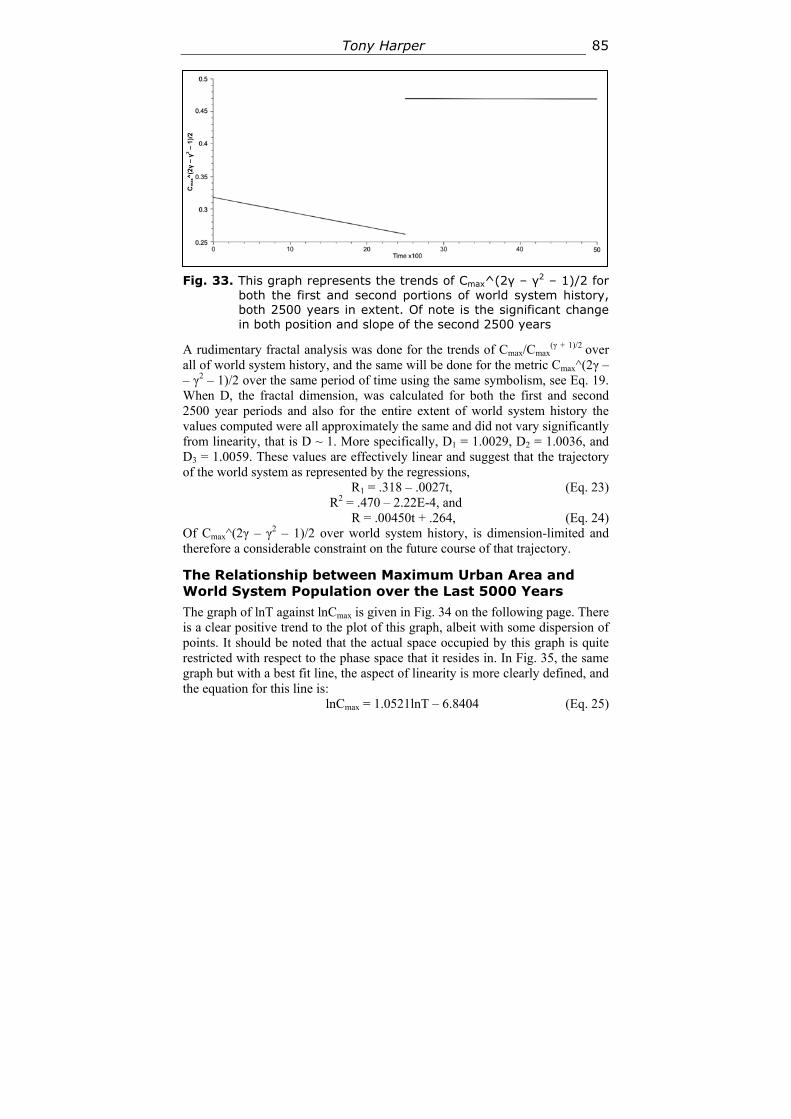
Tony Harper 85
Fig. 33. This graph represents the trends of Cmax^(2γ – γ2 – 1)/2 for
both the first and second portions of world system history, both 2500 years in extent. Of note is the significant change in both position and slope of the second 2500 years
A rudimentary fractal analysis was done for the trends of Cmax/Cmax(γ + 1)/2 over
all of world system history, and the same will be done for the metric Cmax^(2γ – – γ2 – 1)/2 over the same period of time using the same symbolism, see Eq. 19. When D, the fractal dimension, was calculated for both the first and second 2500 year periods and also for the entire extent of world system history the values computed were all approximately the same and did not vary significantly from linearity, that is D ~ 1. More specifically, D1 = 1.0029, D2 = 1.0036, and D3 = 1.0059. These values are effectively linear and suggest that the trajectory of the world system as represented by the regressions,
R1 = .318 – .0027t, (Eq. 23) R2 = .470 – 2.22E-4, and
R = .00450t + .264, (Eq. 24) Of Cmax^(2γ – γ2 – 1)/2 over world system history, is dimension-limited and therefore a considerable constraint on the future course of that trajectory.
The Relationship between Maximum Urban Area and World System Population over the Last 5000 Years
The graph of lnT against lnCmax is given in Fig. 34 on the following page. There is a clear positive trend to the plot of this graph, albeit with some dispersion of points. It should be noted that the actual space occupied by this graph is quite restricted with respect to the phase space that it resides in. In Fig. 35, the same graph but with a best fit line, the aspect of linearity is more clearly defined, and the equation for this line is:
lnCmax = 1.0521lnT – 6.8404 (Eq. 25)
Cm
ax^
(2γ
– γ2
– 1
)/2
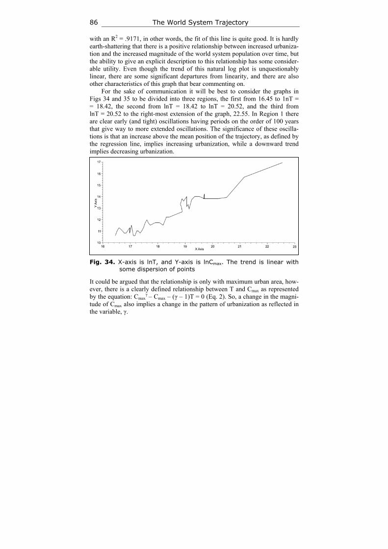
The World System Trajectory 86
with an R2 = .9171, in other words, the fit of this line is quite good. It is hardly earth-shattering that there is a positive relationship between increased urbaniza-tion and the increased magnitude of the world system population over time, but the ability to give an explicit description to this relationship has some consider-able utility. Even though the trend of this natural log plot is unquestionably linear, there are some significant departures from linearity, and there are also other characteristics of this graph that bear commenting on.
For the sake of communication it will be best to consider the graphs in Figs 34 and 35 to be divided into three regions, the first from 16.45 to 1nT = = 18.42, the second from lnT = 18.42 to lnT = 20.52, and the third from lnT = 20.52 to the right-most extension of the graph, 22.55. In Region 1 there are clear early (and tight) oscillations having periods on the order of 100 years that give way to more extended oscillations. The significance of these oscilla-tions is that an increase above the mean position of the trajectory, as defined by the regression line, implies increasing urbanization, while a downward trend implies decreasing urbanization.
Fig. 34. X-axis is lnT, and Y-axis is lnCmax. The trend is linear with
some dispersion of points
It could be argued that the relationship is only with maximum urban area, how-ever, there is a clearly defined relationship between T and Cmax as represented by the equation: Cmax
γ – Cmax – (γ – 1)T = 0 (Eq. 2). So, a change in the magni-tude of Cmax also implies a change in the pattern of urbanization as reflected in the variable, γ.
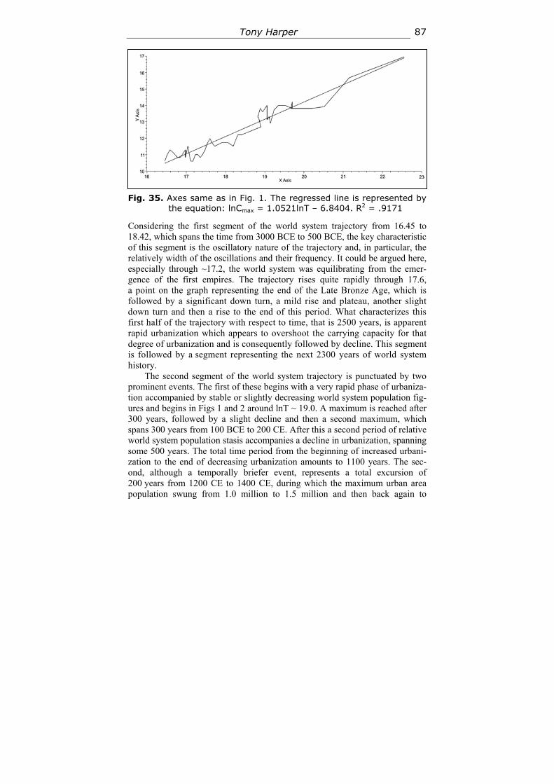
Tony Harper 87
Fig. 35. Axes same as in Fig. 1. The regressed line is represented by
the equation: lnCmax = 1.0521lnT – 6.8404. R2 = .9171
Considering the first segment of the world system trajectory from 16.45 to 18.42, which spans the time from 3000 BCE to 500 BCE, the key characteristic of this segment is the oscillatory nature of the trajectory and, in particular, the relatively width of the oscillations and their frequency. It could be argued here, especially through ~17.2, the world system was equilibrating from the emer-gence of the first empires. The trajectory rises quite rapidly through 17.6, a point on the graph representing the end of the Late Bronze Age, which is followed by a significant down turn, a mild rise and plateau, another slight down turn and then a rise to the end of this period. What characterizes this first half of the trajectory with respect to time, that is 2500 years, is apparent rapid urbanization which appears to overshoot the carrying capacity for that degree of urbanization and is consequently followed by decline. This segment is followed by a segment representing the next 2300 years of world system history.
The second segment of the world system trajectory is punctuated by two prominent events. The first of these begins with a very rapid phase of urbaniza-tion accompanied by stable or slightly decreasing world system population fig-ures and begins in Figs 1 and 2 around lnT ~ 19.0. A maximum is reached after 300 years, followed by a slight decline and then a second maximum, which spans 300 years from 100 BCE to 200 CE. After this a second period of relative world system population stasis accompanies a decline in urbanization, spanning some 500 years. The total time period from the beginning of increased urbani-zation to the end of decreasing urbanization amounts to 1100 years. The sec-ond, although a temporally briefer event, represents a total excursion of 200 years from 1200 CE to 1400 CE, during which the maximum urban area population swung from 1.0 million to 1.5 million and then back again to
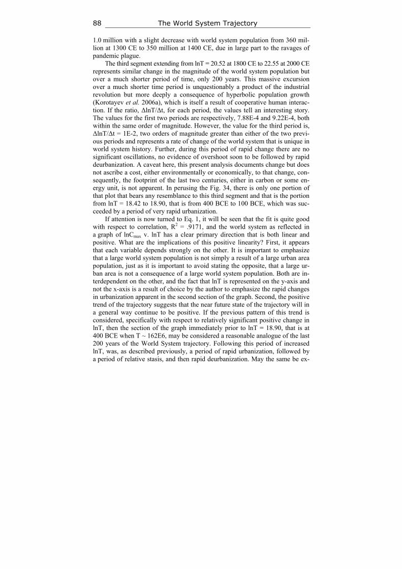
The World System Trajectory 88
1.0 million with a slight decrease with world system population from 360 mil-lion at 1300 CE to 350 million at 1400 CE, due in large part to the ravages of pandemic plague.
The third segment extending from lnT = 20.52 at 1800 CE to 22.55 at 2000 CE represents similar change in the magnitude of the world system population but over a much shorter period of time, only 200 years. This massive excursion over a much shorter time period is unquestionably a product of the industrial revolution but more deeply a consequence of hyperbolic population growth (Korotayev et al. 2006a), which is itself a result of cooperative human interac-tion. If the ratio, ΔlnT/Δt, for each period, the values tell an interesting story. The values for the first two periods are respectively, 7.88E-4 and 9.22E-4, both within the same order of magnitude. However, the value for the third period is, ΔlnT/Δt = 1E-2, two orders of magnitude greater than either of the two previ-ous periods and represents a rate of change of the world system that is unique in world system history. Further, during this period of rapid change there are no significant oscillations, no evidence of overshoot soon to be followed by rapid deurbanization. A caveat here, this present analysis documents change but does not ascribe a cost, either environmentally or economically, to that change, con-sequently, the footprint of the last two centuries, either in carbon or some en-ergy unit, is not apparent. In perusing the Fig. 34, there is only one portion of that plot that bears any resemblance to this third segment and that is the portion from lnT = 18.42 to 18.90, that is from 400 BCE to 100 BCE, which was suc-ceeded by a period of very rapid urbanization.
If attention is now turned to Eq. 1, it will be seen that the fit is quite good with respect to correlation, R2 = .9171, and the world system as reflected in a graph of lnCmax v. lnT has a clear primary direction that is both linear and positive. What are the implications of this positive linearity? First, it appears that each variable depends strongly on the other. It is important to emphasize that a large world system population is not simply a result of a large urban area population, just as it is important to avoid stating the opposite, that a large ur-ban area is not a consequence of a large world system population. Both are in-terdependent on the other, and the fact that lnT is represented on the y-axis and not the x-axis is a result of choice by the author to emphasize the rapid changes in urbanization apparent in the second section of the graph. Second, the positive trend of the trajectory suggests that the near future state of the trajectory will in a general way continue to be positive. If the previous pattern of this trend is considered, specifically with respect to relatively significant positive change in lnT, then the section of the graph immediately prior to lnT = 18.90, that is at 400 BCE when T ~ 162E6, may be considered a reasonable analogue of the last 200 years of the World System trajectory. Following this period of increased lnT, was, as described previously, a period of rapid urbanization, followed by a period of relative stasis, and then rapid deurbanization. May the same be ex-
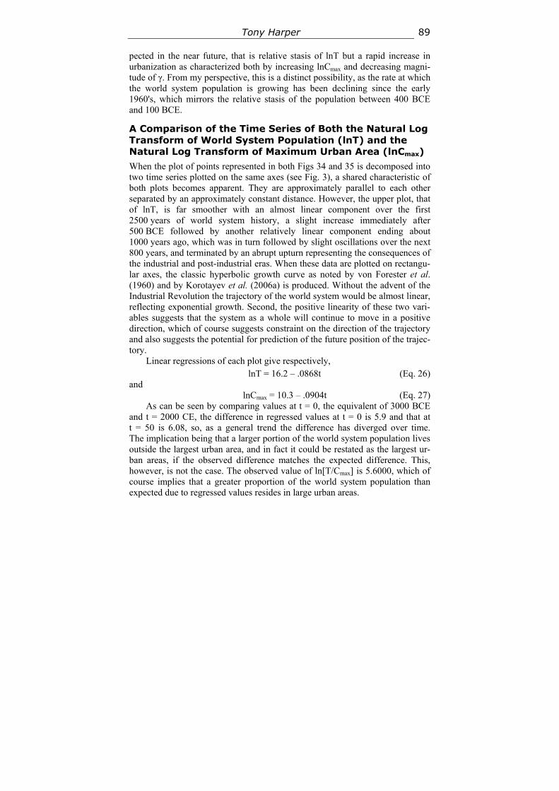
Tony Harper 89
pected in the near future, that is relative stasis of lnT but a rapid increase in urbanization as characterized both by increasing lnCmax and decreasing magni-tude of γ. From my perspective, this is a distinct possibility, as the rate at which the world system population is growing has been declining since the early 1960's, which mirrors the relative stasis of the population between 400 BCE and 100 BCE.
A Comparison of the Time Series of Both the Natural Log Transform of World System Population (lnT) and the Natural Log Transform of Maximum Urban Area (lnCmax)
When the plot of points represented in both Figs 34 and 35 is decomposed into two time series plotted on the same axes (see Fig. 3), a shared characteristic of both plots becomes apparent. They are approximately parallel to each other separated by an approximately constant distance. However, the upper plot, that of lnT, is far smoother with an almost linear component over the first 2500 years of world system history, a slight increase immediately after 500 BCE followed by another relatively linear component ending about 1000 years ago, which was in turn followed by slight oscillations over the next 800 years, and terminated by an abrupt upturn representing the consequences of the industrial and post-industrial eras. When these data are plotted on rectangu-lar axes, the classic hyperbolic growth curve as noted by von Forester et al. (1960) and by Korotayev et al. (2006a) is produced. Without the advent of the Industrial Revolution the trajectory of the world system would be almost linear, reflecting exponential growth. Second, the positive linearity of these two vari-ables suggests that the system as a whole will continue to move in a positive direction, which of course suggests constraint on the direction of the trajectory and also suggests the potential for prediction of the future position of the trajec-tory.
Linear regressions of each plot give respectively, lnT = 16.2 – .0868t (Eq. 26)
and lnCmax = 10.3 – .0904t (Eq. 27)
As can be seen by comparing values at t = 0, the equivalent of 3000 BCE and t = 2000 CE, the difference in regressed values at t = 0 is 5.9 and that at t = 50 is 6.08, so, as a general trend the difference has diverged over time. The implication being that a larger portion of the world system population lives outside the largest urban area, and in fact it could be restated as the largest ur-ban areas, if the observed difference matches the expected difference. This, however, is not the case. The observed value of ln[T/Cmax] is 5.6000, which of course implies that a greater proportion of the world system population than expected due to regressed values resides in large urban areas.
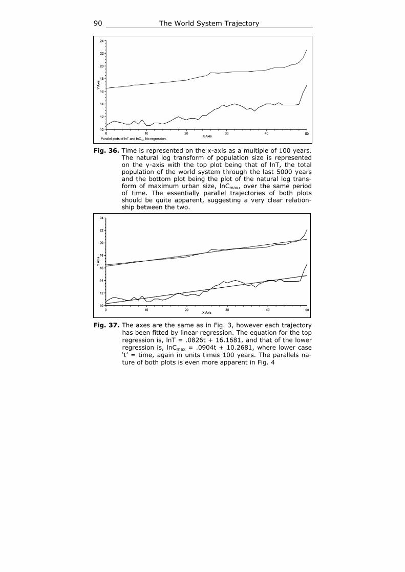
The World System Trajectory 90
Fig. 36. Time is represented on the x-axis as a multiple of 100 years.
The natural log transform of population size is represented on the y-axis with the top plot being that of lnT, the total population of the world system through the last 5000 years and the bottom plot being the plot of the natural log trans-form of maximum urban size, lnCmax, over the same period of time. The essentially parallel trajectories of both plots should be quite apparent, suggesting a very clear relation-ship between the two.
Fig. 37. The axes are the same as in Fig. 3, however each trajectory
has been fitted by linear regression. The equation for the top regression is, lnT = .0826t + 16.1681, and that of the lower regression is, lnCmax = .0904t + 10.2681, where lower case ‘t’ = time, again in units times 100 years. The parallels na-ture of both plots is even more apparent in Fig. 4
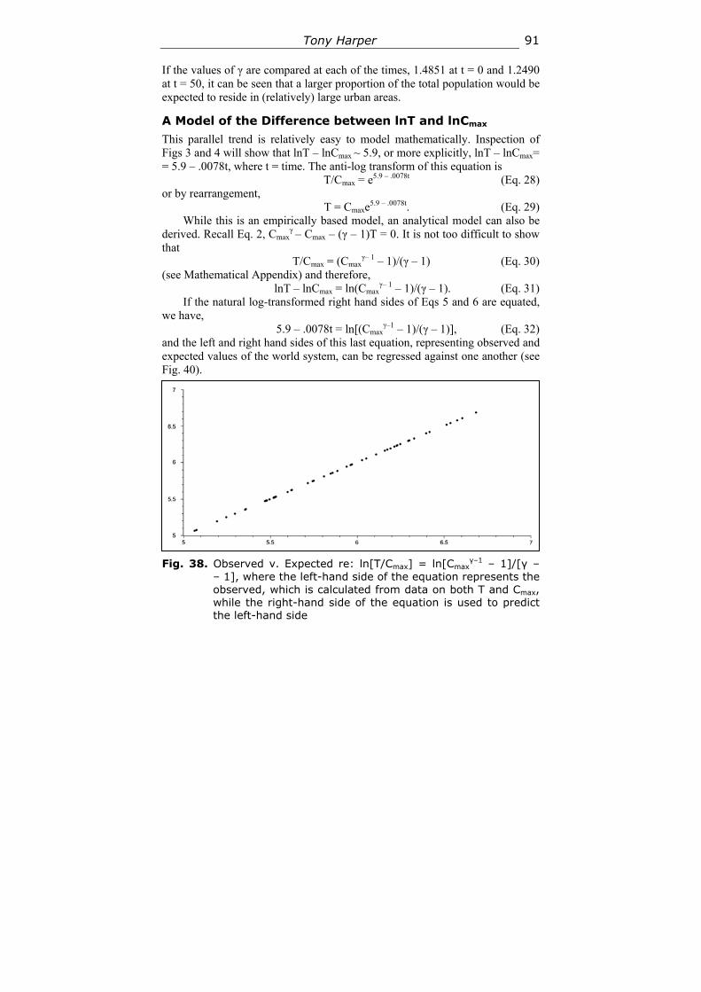
Tony Harper 91
If the values of γ are compared at each of the times, 1.4851 at t = 0 and 1.2490 at t = 50, it can be seen that a larger proportion of the total population would be expected to reside in (relatively) large urban areas.
A Model of the Difference between lnT and lnСmax
This parallel trend is relatively easy to model mathematically. Inspection of Figs 3 and 4 will show that lnT – lnCmax ~ 5.9, or more explicitly, lnT – lnCmax= = 5.9 – .0078t, where t = time. The anti-log transform of this equation is
T/Cmax = e5.9 – .0078t (Eq. 28) or by rearrangement,
T = Cmaxe5.9 – .0078t. (Eq. 29)
While this is an empirically based model, an analytical model can also be derived. Recall Eq. 2, Cmax
γ – Cmax – (γ – 1)T = 0. It is not too difficult to show that
T/Cmax = (Cmaxγ– 1 – 1)/(γ – 1) (Eq. 30)
(see Mathematical Appendix) and therefore, lnT – lnCmax = ln(Cmax
γ– 1 – 1)/(γ – 1). (Eq. 31) If the natural log-transformed right hand sides of Eqs 5 and 6 are equated,
we have, 5.9 – .0078t = ln[(Cmax
γ–1 – 1)/(γ – 1)], (Eq. 32) and the left and right hand sides of this last equation, representing observed and expected values of the world system, can be regressed against one another (see Fig. 40).
Fig. 38. Observed v. Expected re: ln[T/Cmax] = ln[Cmax
γ–1 – 1]/[γ – – 1], where the left-hand side of the equation represents the observed, which is calculated from data on both T and Cmax, while the right-hand side of the equation is used to predict the left-hand side
The World System Trajectory 92
It should be noted here that the above relationship is not unexpected, as Eq. 2 was used to generate values of γ with observed values of both lnT and lnCmax. However, it should also be noted that the left-hand side of Eq. 32 represents an alternative way of finding ln[T/Cmax], one in which the fit is quite good.
Interestingly, the essentially parallel trend of lnT and lnCmax over the last 5000 years suggests that there is a clear link between urbanization and total population growth. This in one sense is unsurprising, however, the contention here and in previous research is that link is in fact γ, the exponent characteriz-ing the distribution of urban size given maximum urban size and total world system population.
The Potential for Prediction
The previous four sections of this paper have addressed the notion of con-straints imposed on the trajectory, the historical trajectory, of the world system over the last 5000 years. A clear general trend with respect to the relationship between γ and lnT has been demonstrated, one that shows a decrease in γ and therefore an increase in the total distribution of the urban population, here de-fined as N ≥ 100, as the natural logarithm of the world system population and therefore the population itself increases. It has been shown that there are spe-cific instances of change in the world system position in reaction to previous system change, e.g., the rapid urbanization of the world system from 400 BCE to 100 BCE followed by a rapid de-urbanization from 200 CE to 500 CE, that suggest that the system is being returned to some steady-state level. The exis-tence of iso-urban lines has been established, lines of similar maximum urban area magnitude with respect to both γ and lnT, and the polar plot of the world system trajectory, the rather tight linearity between H and Ψ, H and time and Ψ and time, the periodicity between the observed and expected of the last two linear relationships, and the ratio of the observed maximum urban area value and the idealized one determined by maximizing Eq. 12a, A = (γ – x)(1 + x). 5lnCmax
2, which reveals that the urbanization of the world system appears to have occurred in two specific regimes, each with a similar rate of occurrence but with differing points of initiation, and which also demonstrates a fractal relationship for the two regimes that is effectively identical. All of these in-stances suggest that the world system is highly constrained, and, in turn, if this is in fact the case, that the behavior of the system, at least at the level of organi-zation implied by the equation, Cmax
γ – Cmax – (γ – 1)T = 0 (Harper 2010b), is (potentially) predictable.
Each of the above constraints will now be given more detailed analysis and explanation and then some discussion will follow with respect to the potential for prediction both in the past, that is retroactively, and for the system as a whole.
To begin, the fact that the linear relationship between γ and lnT has a nega-tive slope suggests in general that for any given position of the world system
Tony Harper 93
future positions from that point on will involve both a decrease in γ and an in-crease in lnT, and over an extended period of time this is unquestionably the case. For example, the position of the world system in 200 CE is one in which the value of γ has decreased as lnT has increased with respect to the world sys-tem position of, say, 2000 BCE. However, if the position of the world system from 200 CE to 300 CE is considered, this is not the case, as there the change involves an increase in γ with no attendant decrease in lnT. In Table 6 below are documented all the changes in both γ and lnT and what this data reveals is that while two relationships predominate, there are several other arrangements between γ and lnT.
Table 6
γ/lnT +/+ +/0 +/– –/– –/0 –/+ Number 22 3 1 2 1 21
As is represented above on a century by century basis then depending where one starts the actual trend of change in γ with respect to lnT may fall into one of six categories.
What is to be made then of the negative slope of the equation γ = 2.23 – .0449lnT? (Eq. 33)
This unquestionably has to be an emergent property of the system itself and as such is only of general predictive value. Of more importance is the fact that the dispersion of points about the trend line is that the greatest variance is approximated by ~.1γ. This fact along with the negative slope have some pre-dictive worth in that bounds are placed on future changes in position of the world system from any previous point. A note of caution here: There are at least two instances in which lnT, and therefore T, the population itself, de-crease, the first during the period of intense urbanization from 300 BCE to 200 BCE and the second from 1300 CE to 1400 CE, the (calamitous) 14th cen-tury, and these population deficits were quite small.
It is to these two specific instances, the period of rapid urbanization at the end of the first millennium BCE and the 14th century and the periods of adjust-ment that followed them, that attention will now be given. Both of these periods of time share the same pattern of development and response, that is both repre-sent periods of intense urbanization directly associated with little or no negative change in total population followed by rapid de-urbanization, in the case of the first period, punctuated by a brief period of de-urbanization followed by a short period of urbanization. It appears then that rapid urbanization constrained by zero world system population growth results in equally rapid de-urbanization, either directly or followed by some relatively short period of time.
To give a numerical explanation for the above phenomenon Eq. 23 from Harper (2010b) was used to calculate the ratio of urbanized population to that of the rural population for the total population. The data are given in Table 7 below.
The World System Trajectory 94
Table 7
γ Cmax Tu/Tr
1.1 2.9E6 1.2803 1.2 1.3E6 .6197 1.3 5.7E5 .3301 1.4 2.7E5 .1876 1.5 1.4E5 .1110 1.6 7.3E4 .0673
Note: The values of Tu/Tr were calculated by Eq. 23 from Harper (2010b): Tu/Tr = = (a(1 – γ) – 1)/(1 – C0
(γ – 1)), where a = Cmax/C0, and C0 = 100.
It can be seen that as γ decreases the proportion of the urbanized population increases. Note that Cmax had to be computed for each γ, and note also that the above table is meant to be a numerical example in which γ was varied over its observed range. This is further represented in Fig. 28 in which γ is plotted against Tu/Tr shows a rapid decline of the urbanized population with respect to increasing γ.
However, the reverse of this trend should actually be considered, as the ur-banization process is associated with decreasing γ. The non-linearity of this process implies a very rapid increase in the proportion of the urbanized popula-tion as suggested by the power relation,
Tu/Tr = 2.81γ–8.41, (Eq. 34) where very rapid urbanization can be expected with smaller and smaller γ. It is my contention that both instances of rapid urbanization followed shortly by rapid de-urbanization, that of the latter part of the last millennium BCE and the 300 years represented by the period of time from 200 CE to 500 CE and also the 13th and 14th centuries CE, are consequences not only of this rapid urbaniza-tion but of the consequences of that urbanization process exceeding some as yet to be defined threshold regarding system wide sustainability. This may well be the process of overshoot and its consequences referred to in the book of the same title Overshoot: The Ecological Basis of Revolutionary Change by Wil-liam R. Catton, Jr.
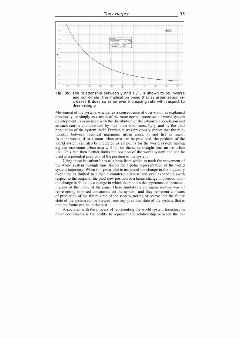
Tony Harper 95
Fig. 39. The relationship between γ and Tu/Tr is shown to be inverse
and non-linear, the implication being that as urbanization in-creases it does so at an ever increasing rate with respect to decreasing γ
Movement of the system, whether as a consequence of over-shoot, as explained previously, or simply as a result of the more normal processes of world system development, is associated with the distribution of the urbanized population and as such can be characterized by maximum urban area, by γ, and by the total population of the system itself. Further, it was previously shown that the rela-tionship between identical maximum urban areas, γ, and lnT is linear. In other words, if maximum urban area can be predicted, the position of the world system can also be predicted as all points for the world system having a given maximum urban area will fall on the same straight line, an iso-urban line. This fact then further limits the position of the world system and can be used as a potential predictor of the position of the system.
Using these iso-urban lines as a base from which to track the movement of the world system through time allows for a polar representation of the world system trajectory. When this polar plot is inspected the change in the trajectory over time is limited to either a counter-clockwise and ever expanding (with respect to the origin of the plot) new position or a linear change in position with-out change in Ψ, that is a change in which the plot has the appearance of proceed-ing out of the plane of the page. These limitations are again another way of representing imposed constraints on the system, and they represent a means of prediction of the future state of the system, noting of course that the future state of the system can be viewed from any previous state of the system, that is that the future can be in the past.
Associated with the process of representing the world system trajectory in polar coordinates is the ability to represent the relationship between the pa-
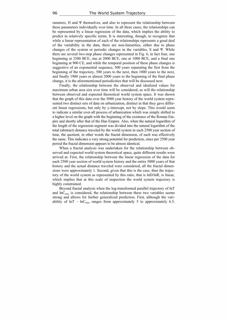
The World System Trajectory 96
rameters, H and Ψ themselves, and also to represent the relationship between these parameters individually over time. In all three cases, the relationships can be represented by a linear regression of the data, which implies the ability to predict in relatively specific terms. It is interesting, though, to recognize that while a linear representation of each of the relationships represents a good deal of the variability in the data, there are non-linearities, either due to phase changes of the system or periodic changes in the variables, S and Ψ. While there are several two-step phase changes represented in Fig. 6, in fact four, one beginning at 2500 BCE, one at 2000 BCE, one at 1000 BCE, and a final one beginning at 900 CE, and while the temporal position of these phase changes is suggestive of an exponential sequence, 500 years separating the first from the beginning of the trajectory, 500 years to the next, then 1000 years to the next, and finally 1900 years or almost 2000 years to the beginning of the final phase change, it is the aforementioned periodicities that will be discussed next.
Finally, the relationship between the observed and idealized values for maximum urban area size over time will be considered, as will the relationship between observed and expected theoretical world system space. It was shown that the graph of this data over the 5000 year history of the world system repre-sented two distinct sets of data on urbanization, distinct in that they gave differ-ent linear regressions, but only by y-intercept, not by slope. This would seem to indicate a similar over-all process of urbanization which was simply shifted to a higher level on the graph with the beginning of the existence of the Roman Em-pire and shortly after that of the Han Empire. Also, when the natural logarithm of the length of the regression segment was divided into the natural logarithm of the total (abstract) distance traveled by the world system in each 2500 year section of time, the quotient, in other words the fractal dimension, of each was effectively the same. This indicates a very strong potential for prediction, since per 2500 year period the fractal dimension appears to be almost identical.
When a fractal analysis was undertaken for the relationship between ob-served and expected world system theoretical space, quite different results were arrived at. First, the relationship between the linear regression of the data for each 2500 year section of world system history and the entire 5000 years of that history and the actual distance traveled were considered, all the fractal dimen-sions were approximately 1. Second, given that this is the case, then the trajec-tory of the world system as represented by this ratio, that is lnD/lnR, is linear, which implies that at this scale of inspection the world system trajectory is highly constrained.
Beyond fractal analysis when the log-transformed parallel trajectory of lnT and lnCmax is considered, the relationship between these two variables seems strong and allows for further generalized prediction. First, although the vari-ability of lnT – lnCmax ranges from approximately 5 to approximately 6.5,
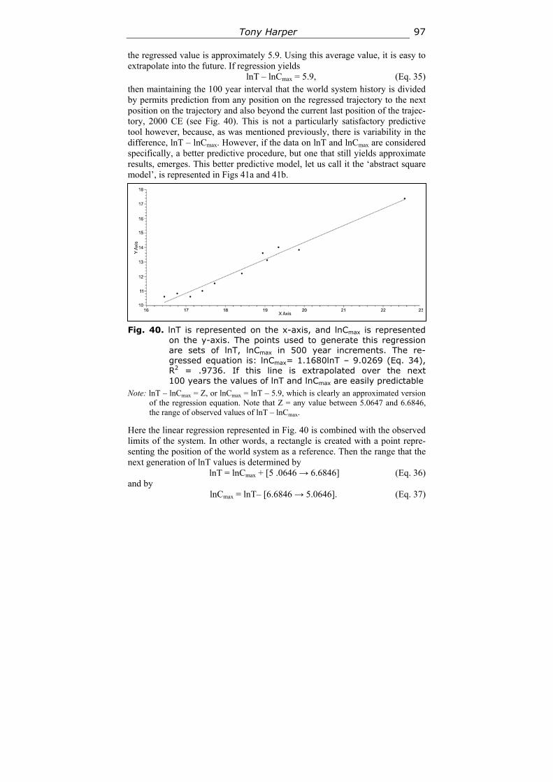
Tony Harper 97
the regressed value is approximately 5.9. Using this average value, it is easy to extrapolate into the future. If regression yields
lnT – lnCmax = 5.9, (Eq. 35) then maintaining the 100 year interval that the world system history is divided by permits prediction from any position on the regressed trajectory to the next position on the trajectory and also beyond the current last position of the trajec-tory, 2000 CE (see Fig. 40). This is not a particularly satisfactory predictive tool however, because, as was mentioned previously, there is variability in the difference, lnT – lnCmax. However, if the data on lnT and lnCmax are considered specifically, a better predictive procedure, but one that still yields approximate results, emerges. This better predictive model, let us call it the ‘abstract square model’, is represented in Figs 41a and 41b.
Fig. 40. lnT is represented on the x-axis, and lnCmax is represented
on the y-axis. The points used to generate this regression are sets of lnT, lnCmax in 500 year increments. The re-gressed equation is: lnCmax= 1.1680lnT – 9.0269 (Eq. 34), R2 = .9736. If this line is extrapolated over the next 100 years the values of lnT and lnCmax are easily predictable
Note: lnT – lnCmax = Z, or lnCmax = lnT – 5.9, which is clearly an approximated version of the regression equation. Note that Z = any value between 5.0647 and 6.6846, the range of observed values of lnT – lnCmax.
Here the linear regression represented in Fig. 40 is combined with the observed limits of the system. In other words, a rectangle is created with a point repre-senting the position of the world system as a reference. Then the range that the next generation of lnT values is determined by
lnT = lnCmax + [5 .0646 → 6.6846] (Eq. 36) and by
lnCmax = lnT– [6.6846 → 5.0646]. (Eq. 37)
The World System Trajectory 98
This gives a square with the dimensions, 1.6199 × 1.6199, in which it is predicted the next generation's world system position can potentially be found. Sadly, this square has within an infinite number of points, which is hardly help-ful. Can probability be used to reduce the possible number of points? Possibly. Note that this square can be subdivided into four different sections, and the sections vary in area suggesting that the probability of the position of the world system falling in any of the subsections is proportional to the area of the sub-section. This is helpful but only in a general way, since each of these rectangu-lar figures has within it an infinite number of points. If the position of the world system is calculated per century with respect to the context of this square, the position of the world system is observed to change, and since this change falls within the zero sum limits of the value, 1.6199, for both axes, then only one variable is necessary to characterize the position of the world system. Specifi-cally, the reference of a zero sum relationship between the position of the world system within the boundaries of the square model imply that if the difference between the position of the world system and the maximum boundary of the square is known, then the other three differences between the other three boundaries are explicitly predictable, because all relationships are dependent on lnT – lnCmax = [6.6846 – 5.0647].
Fig. 41a. This is a simple representation of the general trend of the world system with respect to lnT on the x-axis and lnCmax on the y-axis. In broad terms, the predictability of the future state of the system is simply a matter of following the trend of the line. However, when the range of values between lnT and lnCmax are imposed the number of future positions of the world system becomes more varied as will be seen in Fig. 41b.
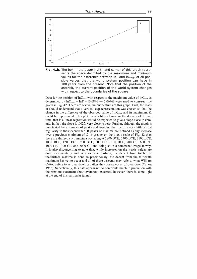
Tony Harper 99
Fig. 41b. The box in the upper right hand corner of this graph repre-
sents the space delimited by the maximum and minimum values for the difference between lnT and lnCmax of all pos-sible values that the world system position can have in 100 years from the present. Note that the position of the asterisk, the current position of the world system changes with respect to the boundaries of the square
Data for the position of lnCmax with respect to the maximum value of lnCmax as determined by lnCmax = lnT – [6.6846 → 5.0646] were used to construct the graph in Fig. 42. There are several unique features of this graph. First, the read-er should understand that a vertical step representation was chosen so that the change in the difference of the observed value of lnCmax and its maximum, Z, could be represented. This plot reveals little change in the domain of Z over time, that is a linear regression would be expected to give a slope close to zero, and, in fact, the slope is .0027, very close to zero. Further, although the graph is punctuated by a number of peaks and troughs, that there is very little visual regularity to their occurrence. If peaks or maxima are defined as any increase over a previous minimum of .2 or greater on the y-axis scale of Fig. 42 then there are thirteen such maxima occurring at 2800 BCE, 2300 BCE, 2100 BCE, 1800 BCE, 1200 BCE, 900 BCE, 600 BCE, 100 BCE, 200 CE, 600 CE, 1000 CE, 1300 CE, and 2000 CE and doing so in a somewhat irregular way. It is also disconcerting to note that, while increases on the y-axis values are done incrementally and in a stepwise fashion, the decent from twelve of the thirteen maxima is done so precipitously; the decent from the thirteenth maximum has yet to occur and all of these descents may refer to what William Catton refers to as overshoot, or rather the consequences of overshoot (Catton 1982). Superficially, this data appear not to contribute much to prediction with the previous statement about overshoot excepted, however, there is some light at the end of this particular tunnel.
*
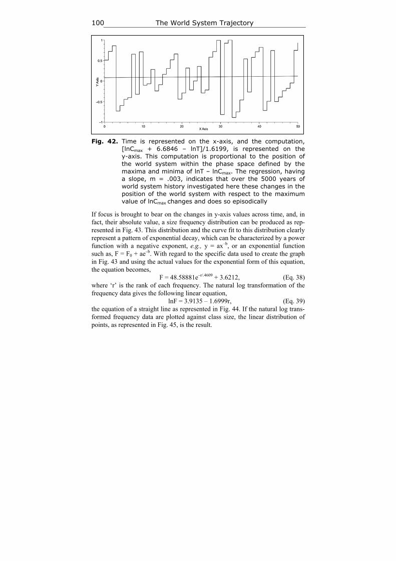
The World System Trajectory 100
Fig. 42. Time is represented on the x-axis, and the computation,
[lnCmax + 6.6846 – lnT]/1.6199, is represented on the y-axis. This computation is proportional to the position of the world system within the phase space defined by the maxima and minima of lnT – lnCmax. The regression, having a slope, m = .003, indicates that over the 5000 years of world system history investigated here these changes in the position of the world system with respect to the maximum value of lnCmax changes and does so episodically
If focus is brought to bear on the changes in y-axis values across time, and, in fact, their absolute value, a size frequency distribution can be produced as rep-resented in Fig. 43. This distribution and the curve fit to this distribution clearly represent a pattern of exponential decay, which can be characterized by a power function with a negative exponent, e.g., y = ax–b, or an exponential function such as, F = F0 + ae–b. With regard to the specific data used to create the graph in Fig. 43 and using the actual values for the exponential form of this equation, the equation becomes,
F = 48.58881e–r/.4609 + 3.6212, (Eq. 38) where ‘r’ is the rank of each frequency. The natural log transformation of the frequency data gives the following linear equation,
lnF = 3.9135 – 1.6999r, (Eq. 39) the equation of a straight line as represented in Fig. 44. If the natural log trans-formed frequency data are plotted against class size, the linear distribution of points, as represented in Fig. 45, is the result.
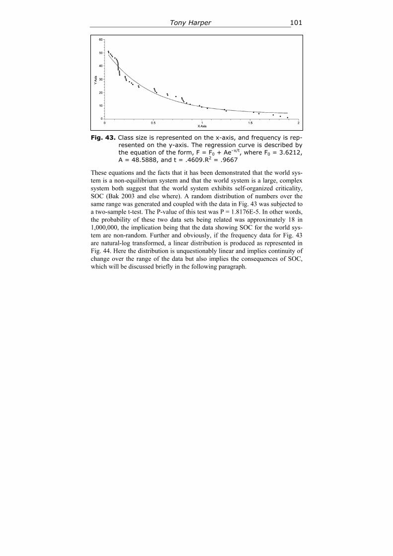
Tony Harper 101
Fig. 43. Class size is represented on the x-axis, and frequency is rep-
resented on the y-axis. The regression curve is described by the equation of the form, F = F0 + Ae–x/t, where F0 = 3.6212, A = 48.5888, and t = .4609.R2 = .9667
These equations and the facts that it has been demonstrated that the world sys-tem is a non-equilibrium system and that the world system is a large, complex system both suggest that the world system exhibits self-organized criticality, SOC (Bak 2003 and else where). A random distribution of numbers over the same range was generated and coupled with the data in Fig. 43 was subjected to a two-sample t-test. The P-value of this test was P = 1.8176E-5. In other words, the probability of these two data sets being related was approximately 18 in 1,000,000, the implication being that the data showing SOC for the world sys-tem are non-random. Further and obviously, if the frequency data for Fig. 43 are natural-log transformed, a linear distribution is produced as represented in Fig. 44. Here the distribution is unquestionably linear and implies continuity of change over the range of the data but also implies the consequences of SOC, which will be discussed briefly in the following paragraph.
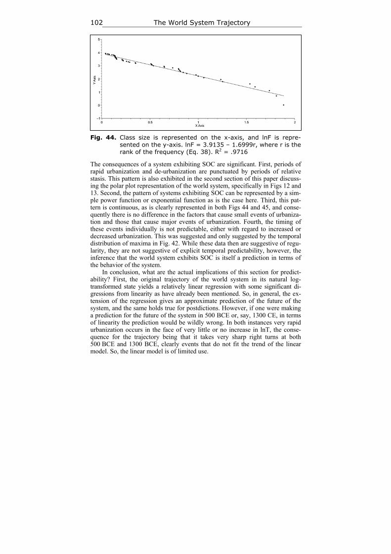
The World System Trajectory 102
Fig. 44. Class size is represented on the x-axis, and lnF is repre-
sented on the y-axis. lnF = 3.9135 – 1.6999r, where r is the rank of the frequency (Eq. 38). R2 = .9716
The consequences of a system exhibiting SOC are significant. First, periods of rapid urbanization and de-urbanization are punctuated by periods of relative stasis. This pattern is also exhibited in the second section of this paper discuss-ing the polar plot representation of the world system, specifically in Figs 12 and 13. Second, the pattern of systems exhibiting SOC can be represented by a sim-ple power function or exponential function as is the case here. Third, this pat-tern is continuous, as is clearly represented in both Figs 44 and 45, and conse-quently there is no difference in the factors that cause small events of urbaniza-tion and those that cause major events of urbanization. Fourth, the timing of these events individually is not predictable, either with regard to increased or decreased urbanization. This was suggested and only suggested by the temporal distribution of maxima in Fig. 42. While these data then are suggestive of regu-larity, they are not suggestive of explicit temporal predictability, however, the inference that the world system exhibits SOC is itself a prediction in terms of the behavior of the system.
In conclusion, what are the actual implications of this section for predict-ability? First, the original trajectory of the world system in its natural log-transformed state yields a relatively linear regression with some significant di-gressions from linearity as have already been mentioned. So, in general, the ex-tension of the regression gives an approximate prediction of the future of the system, and the same holds true for postdictions. However, if one were making a prediction for the future of the system in 500 BCE or, say, 1300 CE, in terms of linearity the prediction would be wildly wrong. In both instances very rapid urbanization occurs in the face of very little or no increase in lnT, the conse-quence for the trajectory being that it takes very sharp right turns at both 500 BCE and 1300 BCE, clearly events that do not fit the trend of the linear model. So, the linear model is of limited use.
Tony Harper 103
A more detailed study of the trajectory reveals that iso-urban lines exist, in other words, that regarding the graph of γ v. lnT points of identical maximum urban area magnitude align linearly. This in itself is of course a prediction. If the current state of the system were to revert to a maximum urban area size of 1,000,000, then the position of the system would fall somewhere on the iso-urban line with m = .0910 and b = –.4430. Consulting Fig. 4 will allow the reader to estimate the current position of the world system if this reversion in maximum urban area size were to occur with no change in lnT. Again, any pre-diction using iso-urban lines would be far from explicit.
In turn, the iso-urban lines were used as a basis for constructing a polar plot of the world system trajectory, an ever expanding spiral subject to the changes in both X = ScosΨ and Y = SsinΨ, the parametric equations for the plot. A three dimensional polar plot reveals a relative degree of regularity in the sys-tem. Given a couple of two-dimensional perspectives, it is quite clear that a rela-tively linear increase in maxima occurs, and the same may be stated for min-ima. Further, when both X and Y are plotted against time their maxima occur in a predictable fashion and, in general, so do the minima. If S and Ψ are plotted against one another, a near-linear plot is achieved, however, there are clear punctuations in this graph in which S changes rapidly while Ψ does not change at all. This behavior of the world system represents punctuations in change al-ternating with relative stasis and is characteristic of a number of biological sys-tems. In itself, this characteristic of the world system is predictive of general, over-all prediction but not explicit prediction.
When maximum urban area size is compared with optimal urban area size a clear trend is revealed with decreasing γ, in that the two values approach one another. The ratio of these two values, Cmax/Cmax
(γ + 1)/2, when plotted against time clearly reveals a disjunct graph, one in which the Ancient World is sepa-rated by a phase change in maximum urban area magnitude from the Classical and Modern Worlds. This phase change occurs during a period of time that roughly coincides with Karl Jasper's Axial Age, but the graph and the data be-hind the graph do not explain why this phase change occurred when it did. It is interesting to note here that the world system may be entering another period of phase change, however, aside from the periodicity of these two events being approximately 2500 years in length, there is little reliance at present that can be placed on a data set of only two events. It is interesting, however, that when a simple fractal analysis is applied to this data that the fractal dimensions of both are nearly identical. This is, in one sense, intellectually comforting, but again does not lend itself to explicit prediction.
When the separate trajectories of both lnT and lnCmax are compared they appear nearly linear and parallel to one another. This is confirmed by calculat-ing the differences between the linear regressions of both trajectories. However, the observed data vary in the difference of their magnitude by 1.6199, a signifi-
The World System Trajectory 104
cant variance when one deals with log-transformed data. While the general re-lationship between lnT and lnCmax is linear, when the variability between lnT and lnCmax makes the prediction within that range of variability for both lnT and lnCmax less possible (see Fig. 41b). Over time the position of the world system varies with respect to the boundaries of the variability. This variability opens the door to a new perspective on the behavior of the world system and the predictability of that behavior.
When this variance in position of the world system with respect to the boundaries of the variance in the difference between lnT and lnCmax is plotted against time and is represented as a vertical series of steps, it is quite clear that the average slope of this graph (Fig. 42.) is nearly zero. But, when a size fre-quency distribution of the absolute values of the vertical steps is constructed, the result is a curve exhibiting decay, which can be represented by either a power function or an exponential function. Given that the world system is a large, com-plex, non-equilibrium system, this result implies that the world system exhibits self-organized criticality. There are three important consequences of this impli-cation. First, the factors that both increase and decrease rates of urbanization are similar for all magnitudes of urbanization. Second, it should be expected that periods of urbanization are episodic. Third, these periods of episodic ur-banization appear not to be temporally predictable.
This research paper closes with two concerns: First, somewhat conflicting data have been presented with regard to the predictability of the world system trajectory as it is understood over the last 5000 years of its history. Unques-tionably, much more research is required to resolve this disparity, however, personally my intuition tells me that further study of the potential for the world system to exhibit SOC, self-organized critically, will be quite productive. Sec-ond, Fig. 43 reveals a pattern of change in which increase in urbanization with respect to the total population of the world system is for the most part done incrementally. However, change in the opposite direction is not, it occurs pre-cipitously. If these data are correct there are two further consequences, that the timing of these down turns is episodic and may not be predictable, and that the magnitudes of the down turns is quite large.
Summary
1. The intent of this paper is to show, first, that the trajectory of the world sys-tem is highly constrained, and, second, that these constraints lead to the possibility of prediction, that is that the position of the world system at any point on its trajec-tory is potentially predictable based on the nature of the constraints analysed.
2. The organization of the world system was described in terms of the rela-tionship between γ, a parameter that generalizes the distribution of urban areas for any given maximum urban area and the total population of the system.
Tony Harper 105
3. Several types of constraint on the world system trajectory were recog-nized. Specifically, the overall trend of the system and the existence of iso-urban lines were discussed.
4. The trajectory of the world system was reconfigured in polar dimensions, the morphology of this plot was described, and the changes over time with re-spect to the polar parameters were noted, and any non-linearities, either of a punctuated or periodic nature were analysed.
5. A standard, the idealized maximum urban area, was established and a ra-tio was generated with the observed maximum urban area divided by the stan-dard. This allowed the recognition of two distinct phases of urbanization and, further, on generating separate regressions for each phase of urbanization it was shown that the fractal dimension of each was essentially the same.
6. As in #5 a standard was established for total potential area of the world system and the actual potential area of the system at each point in time could then be used to generate a ratio of the standard to the actual so that any significant trends in world system activity could be represented. Fractal analysis was per-formed, and it was shown that the fractal dimension for both the 2500 year peri-ods and the entire extent of world system history did not vary significantly from unity. This fact has significance with regard to prediction of the world system trajectory into the future.
7. The parallel trajectories of the world system population as a whole and that of maximum urban areas of that system was analysed, and it was shown that the difference between the natural log-transformed values for both variables falls within a range of values the difference of which is 1.6199.
8. The data on the parallel trajectories of both the natural log-transformed world system population and maximum urban area sizes exhibit properties of self-organized criticality. The consequences of complex systems exhibiting SOC are discussed.
9. The potential of using these constraints and conditions to predict past, present, and future positions of the world system was noted in terms of each of the constraints analysed and each constraint was assessed for its particular contri-bution to understanding the (future) state of the system.
References
Anderson P. W. 1972. More is Different. Science 177: 393–396.
Arrighi G. 1994. The Long Twentieth Century: Money, Power, and the Origins of Our Times. New York: Verso.
Bak P. 1996. How Nature Works. New York: Copernicus Springer-Verlag.
Bak P., Tang C., and Wiesenfeld K. 1987. Self-Organized Criticality: An Explanation of 1/f Noise. Physical Review Letters 59: 381–384.
Catton W. R. Jr. 1982. Overshoot: The Ecological Basis of Revolutionary Change. Chicago, IL: University of Illinois Press.
The World System Trajectory 106
Cohen J. 1995. How Many People Can the Earth Support? New York: W. W. Norton and Company.
von Forester H., Mora P. M., and Amiot L. W. 1960. Doomsday: Friday 13th, No-vember, A.D. 2026. Science 134(3436): 1291–1295.
Grinin L. 2012. Macrohistory and Globalization. Volgograd: Uchitel Publishing House.
Grinin L., and Korotayev A. 2006. Political Development of the World System: A Formal Quantitative Analysis. History and Mathematics. Historical Dynamics and Development of Complex Societies / Ed. by P. Turchin, L. Grinin, A. Korotayev, V. de Munck, pp. 115–153. Moscow: KomKniga/URSS.
Harper T. 2010a. The Macropattern of Urbanization over the Course of the Last 5000 Years of World-System History. Social Evolution & History 9(1): 115–133.
Harper T. 2010b. The Trajectory of the World System over the Last 5000 Years. His-tory and Mathematics: Processes and Models of Global Dynamics / Ed. by L. Grinin, P. Herrmann, A. Korotayev, and A. Tausch, pp. 13–63. Volgograd: Uchitel.
Hutchinson G. E. 1978. An Introduction to Population Ecology. New Haven, CT: Yale University Press.
Korotayev A. 2010. Globalization and Mathematical Modeling of Global Development. Hierarchy and Power: Political Aspects of Modernity / Ed. by L. Grinin, D. Beliaev, and A. Korotayev, pp. 225–240. Moscow: LIBROCOM/URSS.
Korotayev A., and Grinin L. 2006. Urbanization and Political Development of the World System: A Comparative Quantitative Analysis. History and Mathematics: Historical Dynamics and Development of Complex Societies / Ed. by P. Turchin, L. Grinin, V. de Munck, and A. Korotayev, pp. 115–153. Moscow: KomKniga.
Korotayev A., and Grinin L. 2013. Urbanization and Political Development of the World System. Entelequia 5: 197–254.
Korotayev A., Malkov A., and Khaltourina D. 2006a. Introduction to Social Macro-dynamics: Compact Macromodels of the World System Growth. Moscow: URSS.
Korotayev A., Malkov A., and Khaltourina D. 2006b. Introduction to Social Macro-dynamics: Secular Cycles and Millennial Trends. Moscow: URSS.
Korotayev A., Malkov A., and Khaltourina D. 2006c. Introduction to Social Macro-dynamics: Secular Cycles and Millennial Trends in Africa. Moscow: URSS.
Li C. C. 1955. Population Genetics. Chicago, IL: University of Chicago Press.
Malthus T. H. 1798. An Essay on the Principle of Population. The Project Gutenberg. URL: http://www.gutenberg.org/.
Mayr E. 1988. Toward a New Philosophy of Biology: Observations of an Evolutionist. Cambridge: Belknap Press of Harvard University Press.
Modelski G. 2003. World Cities: –3000 to 2000. Cheshire, CT: Faros 2000.
Stavrianos L. S. 1976. The Promise of the Coming Dark Age. San Francisco: W. H. Freeman and Company.

Tony Harper 107
Mathematical Appendix
The Derivation of T/Cmax = (Cmaxγ– 1 – 1)/(γ – 1).
From Eq. 2, Cmaxγ – Cmax – (γ – 1)T = 0, it can be seen that Cmax
γ – Cmax = = (γ – 1)T, and that T = (Cmax
γ – Cmax)/(γ – 1). If Cmax is factored out of the nu-merator and both sides of the equation are divided by Cmax, this will yield: T/Cmax = (Cmax
γ– 1 – 1)/(γ – 1). The Derivation of [e5.9 – .0078t – 1]/[γ e5.9 – .0078t – Cmax
γ – 1] = 1. The linear regressions of lnT and lnCmax yield respectively, lnT = 16.1681 –
– .0826t and lnCmax = 10.2681 – .0904t. Consequently, lnT – lnCmax = 5.9 – – .0078t, and, further, T/Cmax = e5.9 – .0078t. As a result e5.9 – .0078t = [Cmax
γ – 1 – 1]/ [γ – 1] and [γ – 1]e5.9 – .0078t = [Cmax
γ – 1 – 1]. Rearrangement gives: γ e5.9 – .0078t– – Cmax
γ – 1 = e5.9 – .0078t – 1, and dividing both sides by γ e5.9 – .0078t – Cmaxγ – 1
yields: [e5.9 – .0078t – 1]/[γ e5.9 – .0078t – Cmaxγ – 1] = 1.The expected value of this
ratio is clearly 1.0, and the observed value at each 100 year increment can be calculated using appropriate values substituted for each variable of the ratio.
History & Mathematics: Trends and Cycles 2014 108–135
108
3
Another, Simpler Look: Was Wealth Really Determined in 8000 BCE, 1000 BCE, 0 CE,
or Even 1500 CE?
William R. Thompson and Kentaro Sakuwa
Abstract Olsson and Hibbs (2005) and Comin, Easterly, and Gong (2010) make persua-sive theoretical and empirical cases for the persistence of early biogeographi-cal and technological advantages in predicting the distribution of national eco-nomic wealth. However, these results are challenged with an examination of sixteen observations on economic complexity, GDP per capita, and city size spanning as much as ten millennia and eight to eleven regions. The regional complexity / wealth hierarchies are relatively stable only for finite intervals. Early advantages, thus, have some persistence but do not linger indefinitely. The rich do not always get richer or even stay rich, and the poor sometimes improve their standings in the world pecking order dramatically. Early advan-tages are important but need to be balanced with the periodic potential for overriding them.
Keywords: economic growth, early advantage, biogeographical advantage, technological advantage, city size, societal complexity.
Introduction We live in an era fraught with the potential for tectonic changes in relative eco-nomic positioning. The United States, long the leader in technological innova-tion and economic growth, is combating symptoms of relative decline and an increasingly visible challenge from China, a state emerging rapidly from a long period of relative underdevelopment. Japan, thought to be the most like-ly economic challenger to the United States less than two decades ago, is mired in relative stagnant growth and facing a serious population aging problem. Rus-sia, once a challenger to the United States, experienced an economic meltdown when the Soviet Union fragmented. But Russia is re-emerging as an economic competitor of sorts by exploiting the sale of raw materials. A state adjacent to China, India, equally populous, seeks to catch up and surpass China. The region that the United States once overtook, Western Europe, remains affluent but is
William R. Thompson and Kentaro Sakuwa 109
confronted currently with the prospect of the world's one successful regional integration experiment breaking up. Throughout all of these potential changes in the making, a large number of states remain poor and have few prospects for any change in the near, or perhaps distant, future.
It is hardly surprising, then, that the question of how economies grow fast and slow and why some economies get ahead of others while others fall back is popular.1 Many of the arguments that have surfaced focus on more recent de-velopments and yet many of these remain untested empirically. Olsson and Hibbs (2005) and Comin, Easterly, and Gong (2010) are remarkable exceptions to these generalizations. Not only do their studies encompass thousands of years, they go to some lengths to test their perspective on long-term economic growth. Olsson and Hibbs find that Diamond's (1997) argument, predicated on the technological advantages associated with diffusion possibilities linked to continental axes and the distribution of edible plants and large mammals prior to the advent of agriculture, predict well to current national incomes. The strong implication is that the world's distribution of income was deter-mined even before the advent of agriculture. Comin, Easterly, and Gong find that technological adoption in 1500 CE predicts well to national income in the current period and that knowing about the distribution of technology in 1000 BCE and 0 CE predict respectively to technological distributions in 0 CE and 1500 CE. They conclude that the world's distribution of technology has been quite persistent. Wealth distributions, to the extent that they are predicated on technological attainments, were not strictly determined in 1000 BCE but the extent of path dependency is quite strong. Areas that have been technologically ahead in the past tend to continue to be technologically ahead in the present.
Ambitious and largely unprecedented analyses, however, are likely to be characterized by various empirical and design problems. Attempting to capture changes in economic development over thousands of years is never easy or straightforward. Assuming then that there will always be some problems, the question is whether the problems appear to strongly influence the outcome. In this case, the answer is that assumptions made in the research design appear to have biased the conclusions significantly. We do not dispute Olsson and Hibbs (2005) and Comin et al.'s (2010) specific findings as much as what we should make of them. If the central question is whether technological differences per-sist over long periods and the answer lies in the affirmative, there are at least several major caveats that need to be advanced based on the long-term analysis of uneven economic development. By more than tripling the length of the Comin et al.'s examination (from three millennia to ten millennia), expanding the number of observations (to sixteen across the ten millennia), changing the unit of analysis (from contemporary states to regions), and simplifying the indi- 1 In the past decade or so, Diamond (1997), Wong (1997), Frank (1998), Landes (1998), Pomeranz
(2000), Maddison (2001), Clark (2007), Findlay and O'Rourke (2007), Morris (2010, 2013), Ga-lor (2011), Parthasarathi (2011), Rosenthal and Wong (2011), among others, have appeared.
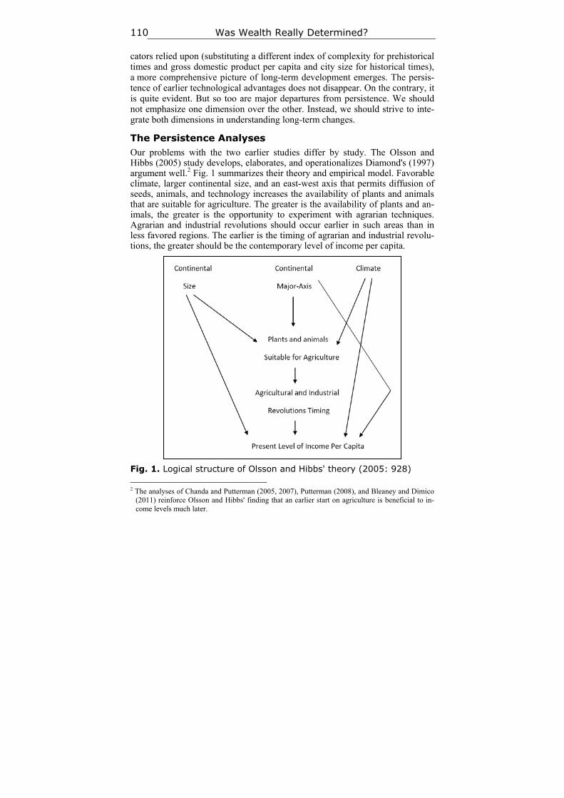
Was Wealth Really Determined? 110
cators relied upon (substituting a different index of complexity for prehistorical times and gross domestic product per capita and city size for historical times), a more comprehensive picture of long-term development emerges. The persis-tence of earlier technological advantages does not disappear. On the contrary, it is quite evident. But so too are major departures from persistence. We should not emphasize one dimension over the other. Instead, we should strive to inte-grate both dimensions in understanding long-term changes.
The Persistence Analyses Our problems with the two earlier studies differ by study. The Olsson and Hibbs (2005) study develops, elaborates, and operationalizes Diamond's (1997) argument well.2 Fig. 1 summarizes their theory and empirical model. Favorable climate, larger continental size, and an east-west axis that permits diffusion of seeds, animals, and technology increases the availability of plants and animals that are suitable for agriculture. The greater is the availability of plants and an-imals, the greater is the opportunity to experiment with agrarian techniques. Agrarian and industrial revolutions should occur earlier in such areas than in less favored regions. The earlier is the timing of agrarian and industrial revolu-tions, the greater should be the contemporary level of income per capita.
Fig. 1. Logical structure of Olsson and Hibbs' theory (2005: 928) 2 The analyses of Chanda and Putterman (2005, 2007), Putterman (2008), and Bleaney and Dimico
(2011) reinforce Olsson and Hibbs' finding that an earlier start on agriculture is beneficial to in-come levels much later.
William R. Thompson and Kentaro Sakuwa 111
One can balk at various aspects of the Diamond argument or not but our main criticism of the Olsson and Hibbs examination is that the tested argument relies on one set of observations.3 Areas favored by geographical size, climate, conti-nental axes that do not block pan-continental diffusion, more large mammals that can be domesticated, and more plants that can be cultivated and consumed will develop earlier. This argument implies that Eurasia will be favored over Africa, Australia, and the Americas – a quite reasonable starting point for eco-nomic growth analyses.4 It helps to explain, for instance and with some sub-stantial help from the spread of European diseases to the Americas, why Span-ish conquistadors could defeat the Aztecs and Incas.5 It does not really specify why different parts of Eurasia have fared much differently on economic devel-opment criteria – a topic on which Diamond (1997) waffles.6 Nor does it ex-plain why Eurasia writ large has not linearly developed faster than Africa, Aus-tralia, and the Americas. Thus, if we use observations based on ten thousand years ago to predict to the present, we skip much of what happened (or may have happened) in between.7
The Comin et al.'s analysis (2010) looks at some of the things that hap-pened in between the advent of agriculture and the contemporary period but there are at least six problematic sources of bias. The first problem is ignored almost entirely by the 2010 analysis. From the most macroscopic vantage point conceivable, economic development was first manifested most spectacularly in Sumer, and, later, Egypt and the eastern Mediterranean. The structural axis of Eurasian growth then was transformed into a ‘dumb-bell’ shape with the Medi-terranean on one end and China on the other. Both dumb-bell ends went into
3 See Acemoglu and Johnson (2012: 51–56), among others, for a critique of the Diamond argument.
Olsson and Paik (2012) develop and test a very interesting argument about the timing of agricul-ture that substantially modifies the idea of early biogeographical advantages. Basically, the idea is that the earliest adopters of agriculture tended also to adopt highly autocratic political systems which subsequently led to poor or poorer than might otherwise have been anticipated economic performance. Later adopters tended to develop different, less extractive, institutions and, there-fore, enjoyed better economic development.
4 See Turchin and Hall (2006) for an extension of the argument to imperial development. 5 There is no question that Eurasia is the largest populated continent and that it encompasses more
plants and large mammals that can be used for economic development purposes. Unlike the north-south alignment of Americas and Africa with major, mid-continental blockages to diffusion, it is not only possible for plants, animals, and technological innovations in one end of Eurasia to travel to the other; it is difficult to account for Eurasian development without tracking the diffusions. Parts of Eurasia certainly experienced earlier agricultural and industrial revolutions than else-where.
6 At one point, Diamond (1997) suggests that any part of Eurasia might have seized the develop-ment lead but later suggests that western Eurasia was favored over eastern Eurasia.
7 Actually, Olsson and Hibbs (2005) say that their initial observations are based on 11,000 BCE because it is around this time that unequal levels of development began to emerge due to popula-tion migrations that had started in Africa some 70,000 years earlier and climate change that melt-ed glaciers thereby making agriculture possible in the northern hemisphere.
Was Wealth Really Determined? 112
decline around the same time but China re-emerged more strongly in the Sui/T'ang/Song era (roughly 8th–13th centuries CE) than did the Mediterranean, although the dumb-bell structure was initially rebuilt in terms of exchanges between the now-Islamic Middle East and China. China then stagnated, thanks in large part to the Mongol takeover, but its economic innovations were dif-fused across Eurasia to Europe thereby establishing a foundation for subsequent industrial revolutions that catapulted first Britain and then other parts of Europe into the economic lead after the 18th century CE. More recently, a few areas settled by British and European migrants in large numbers have moved ahead of Europe in terms of technological development and economic wealth.
Most of this story makes some tangential appearance in the Comin et al. discussion but it does not figure very prominently in the analysis or conclu-sions. If technology advantages are persistent, why did the Persian Gulf area (Sumer) not maintain its lead? Why did the Rome-Han exchange between the two most advanced parts of the world collapse? Why did China surge ahead only to stagnate in the same period Europe was catching up and forging ahead? Why was Europe the initial beneficiary of industrial revolution but later eclipsed by the United States? Put differently, why did some European colonies out-perform their one-time metropoles? We have various answers for these questions, although many remain contested areas of inquiry. Comin et al. (2010) concentrate primarily on the role of European migration in the post-1500 period which helps to answer one of the questions (the near-contemporary and highly selective, colonial catch up with the metropoles) but do not really address the earlier historical questions.
The problem here is that the European migration to less populated North America and Australia / New Zealand was a fairly unique phenomenon.8 We know a fair amount about how and why a few of the colonies attracted a dis-proportionate share of migrating labor and how that was then parlayed into dis-proportionate shares of international capital investment and global trade inte-gration, in conjunction with optimal locations (in terms of climate and oceans) and natural endowments.9 But while large-scale migrations did occur in earlier periods, they cannot explain the decline of Sumer, Egypt, Rome, Han China in ancient history or the fall of various empires in medieval history.10
8 Perhaps the main exceptions are the ‘out of Africa’ movements 50 to 100, 000 years ago in which
our species colonized the world and Greek and Phoenician colonization in the first millennium BCE.
9 See, for instance, the analyses reported in Acemoglu, Johnson, and Robinson (2001, 2002); Sachs, Mellinger, and Gallup (2001); and Krieckhaus (2006).
10 In some of these cases, migrations of ‘barbarian’ tribes are part of the decline explanations. How-ever, it is easier to argue that imperial decline or weaknesses attracted the migrations and that be-cause of the decline, the migrations were more difficult to manage than it is to contend that mi-grations were either the or a principal cause of the decline. Yet many of the countless tribal mi-grations did not involve individuals with technological skills moving into low-tech environments.
William R. Thompson and Kentaro Sakuwa 113
The second bias is that the analysis hinges on comparing observations at only three time points – 1000 BCE, 0, and 1500 CE. If the analysis is to be re-stricted to three observations, analysts need to be careful that the selected ob-servations are relatively neutral in their implications for economic growth as-sessments. The three chosen by Comin et al. are not exactly neutral. Towards the end of the second millennium BCE, the most economically advanced cen-ters in the world were located in the eastern Mediterranean littoral and China. The initial observation date, 1000 BCE, encompasses a period of ‘dark age’ depression in the Mediterranean area that had begun around 1200 BCE and lasted roughly through 800 BCE. The depression in economic and population growth had been brought on by a combination of extensive drought, massive migrations, urban destruction, and considerable conflict. China was not in much better shape. The Western Chou regime in this time period was retreating from tribal pressures in the west, becoming the Eastern Chou regime in the process, and initiating a period of fragmentation that led to the Warring States era in the second half of the first millennium BCE. The year 0 is a bit of a chronological contrivance but, in marked contrast to 1000 BCE, it captures the high points of the Roman and Han empires, ostensibly the economic growth leaders of the ancient world. The third observation point, 1500 CE, of course, passes over a millennium and a half of interesting developments vis-à-vis relative economic growth but it also marks more or less the starting point of European oceanic voyaging. If one of the main indicators of technological growth for this time period is ships with guns and only one small corner of the world has ships with guns in 1500, the observation point is hardly neutral.11 For example, if the same indicator had been used in, say, 1400 CE, merely a hundred years earlier, only China then possessed ships with guns. Europeans were still limited to firing arrows from their ships at that time.
A third problem is associated with the unit of analysis. Comin et al. (2010) carry out most of their analyses examining 104–130 current states and backdat-
It was often the other way around although tribal warriors did sometimes possess superior weap-onry technology – as illustrated by the Hyksos early second millennium BCE movement into Egypt with chariots and stronger bows. However, exceptions on the order of the Phoenician founding of Carthage certainly occurred.
11 One of the Comin et al. (2010) technology indicators for 1500 is ships with 180+ guns. It seems highly unlikely that any ship in the world carried (or could carry without sinking) 180 guns or cannon as early as 1500. At this time, Portuguese ships were armed with artillery that more close-ly resembled mortars more than cannons but the naos were fairly small and only a few pieces of artillery could be carried on board ship. On the other hand, if the opposition possessed no mari-time artillery, as in the Indian Ocean, a few guns often (but not always) sufficed. Henry VIII of England did have several very large ships constructed in the second decade of the 16th century and at least one (The Great Harry) carried 184 guns. But most of these guns were too small to do damage to ships and were used to repel boarders. The ships proved hard to sail, at least one cap-sized in part due to the heavy guns carried, and by the 1530s, the surviving ships were carrying fewer guns. See Hogg and Batchelor (1978: 11) and Archer et al. (2002: 262–263).
Was Wealth Really Determined? 114
ing their attributes based on geographic location. The awkwardness here is that earlier observations are based to some extent on prominent empires. All current states that were once located in the Roman Empire, for instance, receive the same score in the year 0. That means Libya, Syria, Romania, France, and the United Kingdom are scored exactly the same. More generally, empires tended to cover large territories in which some areas were more economically ad-vanced than were others. The Comin et al.'s approach treats imperial peripher-ies as equivalent to imperial centers. It also implies that imperial technologies persisted. In some senses, they did as exemplified by roads and canals that were modified over the years. In other respects, however, the technologies survive only in the form of scattered ruins that attract curious tourists.
Relying on the Peregrine (2003) Atlas of Cultural Evolution source for coding technology creates a fourth problem.12 The Atlas of Cultural Evolution (ACE), a database that provides systematic information on societal complexity in all prehistorical areas, is indispensable for places less well known. Yet once an area moves from prehistorical to historical, ACE ceases to code its complex-ity levels. If one begins an analysis in 1000 BCE, a respectable part of the an-cient world has already moved beyond the ACE codings which were designed mainly for earlier, less developed, pre-written history circumstances. Using ACE in the year 0 is even more difficult to defend.
All efforts to enumerate technology run into the problem of filtering what is included and excluded. For instance, more recent efforts to measure the pace of change in industrial innovation, on occasion, have given equal weight to ball point pens as they do to jet engines.13 Ball point pens and jet engines do not figure in the Comin et al.'s study but they do abandon ACE for the 1500 CE observation and apply a 24 item scale to measure technological development. However, a fifth source of problems concerns the fact that eight of the twenty-four indicators are military in nature. They include standing army, cavalry, fire-arms, muskets, field artillery, warfare capable ships, heavy naval guns, and ships with 180+ guns. Are these indicators of technology or military power? If the latter, the more straightforward interpretation, the explanation has been al-tered substantially. Is it military technology that predicts to contemporary eco-nomic wealth? It is not clear, moreover, why some things are double- or triple-counted (two measures of firearms and three measures of naval capability for instance).14 Another three indicators in the transportation category capture ships
12 ACE is based on the nine-volume Encyclopedia of Prehistory (Peregrine and Embers 2001). 13 See, for instance, the list of innovations examined in van Duijn (1983: 178). 14 While there is no reason to spend a great deal of time on a single indicator, the technological
significance of cavalry, at least on or after 1500, is questionable. At one point, the adoption of cavalry and, later, the stirrup, reflected significant changes in military technology but in places that had access to horses these changes long preceded 1500 CE. Central Eurasian nomads led the way but did not necessarily create standing cavalries. Assyrians began to emulate their practices
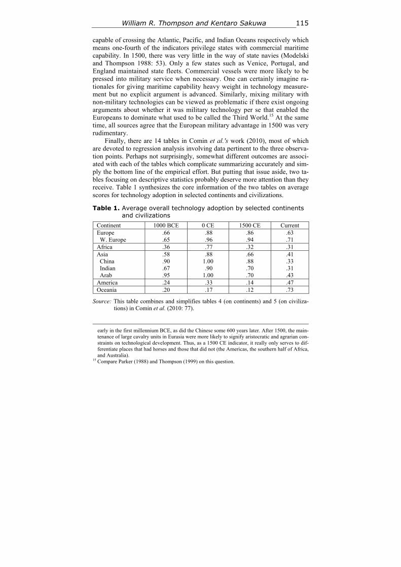
William R. Thompson and Kentaro Sakuwa 115
capable of crossing the Atlantic, Pacific, and Indian Oceans respectively which means one-fourth of the indicators privilege states with commercial maritime capability. In 1500, there was very little in the way of state navies (Modelski and Thompson 1988: 53). Only a few states such as Venice, Portugal, and England maintained state fleets. Commercial vessels were more likely to be pressed into military service when necessary. One can certainly imagine ra-tionales for giving maritime capability heavy weight in technology measure-ment but no explicit argument is advanced. Similarly, mixing military with non-military technologies can be viewed as problematic if there exist ongoing arguments about whether it was military technology per se that enabled the Europeans to dominate what used to be called the Third World.15 At the same time, all sources agree that the European military advantage in 1500 was very rudimentary.
Finally, there are 14 tables in Comin et al.'s work (2010), most of which are devoted to regression analysis involving data pertinent to the three observa-tion points. Perhaps not surprisingly, somewhat different outcomes are associ-ated with each of the tables which complicate summarizing accurately and sim-ply the bottom line of the empirical effort. But putting that issue aside, two ta-bles focusing on descriptive statistics probably deserve more attention than they receive. Table 1 synthesizes the core information of the two tables on average scores for technology adoption in selected continents and civilizations.
Table 1. Average overall technology adoption by selected continents and civilizations
Continent 1000 BCE 0 CE 1500 CE Current Europe W. Europe
.66
.65 .88 .96
.86
.94 .63 .71
Africa .36 .77 .32 .31 Asia China Indian Arab
.58
.90
.67
.95
.88 1.00 .90 1.00
.66
.88
.70
.70
.41
.33
.31
.43 America .24 .33 .14 .47 Oceania .20 .17 .12 .73
Source: This table combines and simplifies tables 4 (on continents) and 5 (on civiliza-tions) in Comin et al. (2010: 77).
early in the first millennium BCE, as did the Chinese some 600 years later. After 1500, the main-tenance of large cavalry units in Eurasia were more likely to signify aristocratic and agrarian con-straints on technological development. Thus, as a 1500 CE indicator, it really only serves to dif-ferentiate places that had horses and those that did not (the Americas, the southern half of Africa, and Australia).
15 Compare Parker (1988) and Thompson (1999) on this question.
Was Wealth Really Determined? 116
Table 1 demonstrates a simple pattern. All areas indicated a peak in the year 1 and then decline. The Europeans decline least. The Americans and Oce-anians make a comeback in the current time period while Africans and Asians are showing as continuing to decline. Whether or not this pattern makes histori-cal sense, it suggests that there are very real limits to the technological persis-tence argument. If the data are ‘right’, we need to explain what happened to China, India, and the Arabs, all of whom were technological leaders at one time and then far from it at other, later times, especially after 1500. Table 1 suggests that the question should not be one of asking whether technological advantages persist in general, but why are they sometimes lost and sometimes gained.
A Different Approach and Indices
We prefer to follow up on the tantalizing simplifications of Table 1. We first recreate a Diamond/Olsson-Hibbs index for a very early biogeographical ad-vantage. Using ACE data on development complexity for four observations: 4000 BCE, 3000 BCE, 2000 BCE and 1000 BCE, we then switch to Maddi-son's data on gross domestic product (GDP) per capita which begins in year 1 CE and continues through 1000 CE, 1500 CE, 1600 CE, 1700 CE, 1820 CE, 1870 CE, 1913 CE, 1950 CE, 1973 CE, and 2003 CE. Sixteen observations should be better than one or three. Rather than attempt to create a different technology scale for each observation, we rely primarily on summary bio-geographical and ACE indexes for the BCE period and a standardized index of economic development for the CE era.
Instead of looking at current countries, we use calculations for 8 ‘regions’ (Western Europe, Eastern Europe, the USSR, Asia, Japan, Latin America, Af-rica, and the Western Offshoots) that remain the same from 8000 BCE to 2003 CE. There is no claim made here that either regions in general or these particular regional identifications are ideal units of analysis. Maddison's aggre-gations are more than a bit idiosyncratic. Yet using his older data means using his choice of aggregations because dis-aggregated numbers are not made avail-able. They do offer, however, several advantages. Regions could be said to more closely approximate ancient empires than do countries, although there is distortion either way.16 Current regions do at least resemble ancient regions with little distortion. Maddison (2007: 382) makes regional GDP per capita data available back to the year 1. One can certainly argue that the data are fab-rications but an effort has been made to justify and standardize them as mean-ingful and systematic fabrications. Moreover, Maddison (1995: 21) raised a similar issue to the present concern by stressing that the regional hierarchy of
16 Switching from states to regions does not eliminate the center-periphery problem but there does
seem to be some tendency for regions to become more homogenous over time in terms of existing levels of economic development.
William R. Thompson and Kentaro Sakuwa 117
economic growth performance changed very little since 1820. The regions that were ahead in 1820 have remained ahead. Similarly, the regions in the hierar-chical cellar were still at the bottom nearly 200 years later. This affords us with the opportunity to not only re-address Comin et al.'s persistence question with Maddison's data but to also extend Maddison's version of the persistence question backwards in time to 8000 BCE. If the regional hierarchy has been sta-ble for the past two centuries, can we say the same for the past ten millennia? If the hierarchy is more stable in the ‘short-term’ (i.e., centuries) than it is in the long-term (millennia), what does that tell us about technological persistence?
One disadvantage of the Maddisonian regional approach is that it does dis-tort ancient history in the sense that the regions with which we are familiar to-day, and the ones Maddison relied on, were regions before but they were not as important as regions as they have since become. To give full justice to ancient history, we would prefer data on Sumer to the Middle East (also not in Maddi-son's geographical lexicon), Indus to India, or China to Asia.17 Maddison's re-gions become more awkward and heterogeneous the farther back in time we go but there is little choice once a decision has been made to utilize Maddison's GDP per capita constructions and wed them with ACE complexity scores in order to encompass ten millennia.18
Switching to GDP per capita also obscures the Comin et al.'s emphasis on technology somewhat.19 A more straightforward measure of technology across time would be preferable but hard to imagine. With sixteen observa-tions across ten millennia, one would have to create a new technological com-plexity scale for each observation. While it might be possible to do that, it seems preferable to simplify the task by relying on ACE indices for the BCE period and Maddison's index for the CE era. Relying on GDP per capita as a crude proxy for technological complexity is certainly not uncommon. Yet these indicator simpli-fications only suggest that our interpretation of the problem will not be the last word on the subject, any more than was Olsson and Hibbs' (2005) or Comin et al.'s (2010).20
At the same time, we can examine this question of path dependency in an entirely different way and one that avoids the problems associated with us-ing Maddison's data. If Maddison's regions are thought to be idiosyncratic and 17 Maddison seems to have preferred to ignore the Middle East as much as possible in his data
collection efforts. Presumably, that tendency reflects a desire to evade the problems associated with small, oil rich states and, perhaps, poor data for the poorer members of that region. To the extent that he dealt with this region, it is usually considered as a western extension of Asia. He classifies Egypt as an African state.
18 That is to say that Maddison's older data are not available independent of his regional aggrega-tions.
19 Yet consider Comin et al.'s (2010). 20 However, see as well the very strong correlations we find between regional GDP per capita and
regional technological standings and report in the Appendix.
Was Wealth Really Determined? 118
highly heterogeneous and his older GDP per capita estimates are difficult to verify, we can avoid these liabilities by examining city size data regionally ag-gregated in more discrete geographical aggregations. City size data (Chandler 1987 and Modelski 2003) are available back to the beginning of cities and the assertion that regions with more large cities are/were wealthier and more tech-nologically advanced than regions with fewer large cities seems easy to ad-vance. Networks of cities, after all, have provided the basic infrastructure of the world economy for millennia.21 All large cities do not work exactly the same. Some have served as agrarian hubs while others represent coastal, commercial nodes. But economic development historically has been manifested in the ur-banized centers of political-economic wealth and power ever since the rise of Sumer and extending to the Pax Britannica and Americana, centered on London and New York, respectively. The only caveat is that this argument can no long-er be sustained in the contemporary era due to the emergence of very large third world cities that confuse the issue of what large cities currently represent.
To operationalize this alternative, we isolate the 25 largest cities between 3700 BCE and 1950 CE at 23 points of observation.22 Each city is assigned to one of eleven regions; Mesopotamia/Iran, Southern Mediterranean (extending from Constantinople to Morocco), Northern Mediterranean / Western Europe (initially extending from Greece to Spain and later farther north), South Asia (primarily the areas that became Pakistan and India), Central Asia (encompass-ing states now designated as ‘stans’ except for Pakistan), Eastern Europe (east of Berlin and Vienna and including what became Russia), Southeast Asia (es-sentially the areas that became Burma/Myanmar to Vietnam and south), East Asia (encompassing China, Korea, and Japan), North America (basically the United States), Central America (basically Mexico), and South America (the continent south of what is now Panama).23
Once a city is assigned to a region, its population is aggregated with other cities in the same region.24 Each region's relative share of the total population of the top twenty-five cities then serves as an indicator of its relative regional standing. Initially, the Mesopotamian/Iranian region monopolizes the large cit-
21 On this subject, see Chase-Dunn and Willard (1994); Chase-Dunn, Manning, and Hall (2000);
Chase-Dunn and Manning (2002); Modelski (2003); and Chase-Dunn, Hall and Turchin (2007). 22 Choosing to look only at the top 25 is arbitrary but in older periods, cities tend to become fairly
small as one moves beyond the first 25. Restricting our focus to the top 25 thus reduces some of the noise that might be introduced by casting the net farther down the size line. It also helps that Chandler (1987) provides more locational information for the first 25. However, Chandler identi-fies sources of imperial control whereas we are focused on geographical location.
23 There are a small number of large cities that do not fit in any of these regions (for instance, a few cities rise to make the top twenty-five threshold in the Arabian Peninsula) but their relative prom-inence tends to be too short-lived to expand the number of regions.
24 Only one city changes its regional location. We code Constantinople as Northern Mediterranean prior to the arrival of the Ottoman Turks and Southern Mediterranean thereafter.
William R. Thompson and Kentaro Sakuwa 119
ies but urbanization gradually diffuses to the east and west. Some regions, such as East Asia, fluctuate in significance while others attain significance only early or late. Our question is whether knowing something about the relative standing of a region at one point in time is very useful in predicting its standing at suc-cessive points in time.
Creating a biogeographical index within the context of Maddison's regions requires some adjustments. To be faithful to the Diamond/Olsson and Hibbs argument, the maximal set of ingredients for such an index should include ob-servations for climate, continental size, continental axis direction, numbers of large mammals and plants that were domesticated, and the onset of agriculture. But if we are differentiating within continents (Maddison has five Eurasian regions: Western Europe, Eastern Europe, the former Soviet Union, Asia, and Japan), continental size is no longer an issue. Climate is another casualty be-cause most regions in our study are characterized by very different climate zones.25
Differentiating east-west axes (Eurasia) from north-south axes (Americas, Africa, and Australia) is not difficult.26 Olsson and Hibbs (2005) provide in-formation on plants and large mammals for most of the regions, as indicated in Table 2. Dates on the timing of agricultural revolutions in specific areas can be linked to regional locations without too much distortion. The dates in parenthe-ses are estimates based on discussion of the spread of agriculture to areas in which it did not originate (Smith 1995; Imamura 1996; Thomas 1996; Frachetti et al. 2010). To create a single biogeographical index, the binary axis informa-tion is scored as 5 points if a region is in the vicinity of the Eurasian east-west axis and 0 points if the region is not located within Eurasia. The distribution of plants and mammals is trichotomized as high (Western and Eastern Europe), medium (Asia and the former Soviet Union), and low (all other regions). High scores were assigned 10 points, the medium scores received 6 points, and low scores were turned into 2 points.27 For the agricultural revolution timing,
25 Another problem is that some regions have experienced climate changes over the last ten millen-
nia. See, e.g., Burroughs (2005). 26 A reviewer, contrary to Diamond, has argued that Africa has a long east-west axis stretching
across the Sahel to the Horn. We do not find this axis very compelling because of the difficulties in crossing (we know French soldiers had problems making the crossing to set up the 1898 Fa-shoda crisis) and the limited historical traffic actually traversing it (at best, presumably, small groups of desert nomads). More important, large and urbanized population centers at both ends, which may be the most critical factor in differentiating between east-west and north-south inter-actions even though it goes beyond the Diamond argument, are missing in the African case. Eur-asia's east-west axis was not all that easy to traverse but traders at least had strong profit incen-tives to make the effort. Just how important people were as carriers to the diffusion of seeds and animals across Eurasia is not entirely clear. Nonetheless, we will check our results to see how critical the presence or absence of an African east-west axis is to the outcome.
27 We did not give equal weight to the continental axis and plants/mammals indicators because Eurasia already scores relatively highly on the distribution of domesticated flora and fauna. In
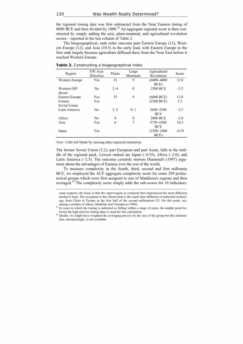
Was Wealth Really Determined? 120
the regional timing date was first subtracted from the Near Eastern timing of 8000 BCE and then divided by 1000.28 An aggregate regional score is then con-structed by simply adding the axis, plant-mammal, and agricultural revolution scores – reported in the last column of Table 2.
The biogeographical, rank order outcome puts Eastern Europe (13), West-ern Europe (12), and Asia (10.5) in the early lead, with Eastern Europe in the first rank largely because agriculture diffused there from the Near East before it reached Western Europe.
Table 2. Constructing a biogeographical index
Region EW Axis Direction
Plants Large
Mammals Agricultural Revolution
Score
Western Europe Yes 33 9 (6000–4000 BCE)
12.0
Western Off-shoots
No 2–4 0 2500 BCE –3.5
Eastern Europe Yes 33 9 (6000 BCE) 13.0 Former Soviet Union
Yes (2200 BCE) 5.2
Latin America No 2–5 0–1 2600–2500 BCE
–2.5
Africa No 4 0 2000 BCE –2.0 Asia Yes 6 7 5750–6500
BCE 10.5
Japan Yes (2500–2400 BCE)
–0.55
Note: Cells left blank by missing data required estimation.
The former Soviet Union (5.2), part European and part Asian, falls in the mid-dle of the regional pack. Lowest ranked are Japan (–0.55), Africa (–2.0), and Latin America (–2.5). The outcome certainly mirrors Diamond's (1997) argu-ment about the advantages of Eurasia over the rest of the world.
To measure complexity in the fourth, third, second and first millennia BCE, we employed the ACE aggregate complexity score for some 289 prehis-torical groups which were first assigned to one of Maddison's regions and then averaged.29 The complexity score simply adds the sub-scores for 10 indicators:
some respects, the irony is that the super-region or continent that experienced the most diffusion needed it least. The exception to this observation is the much later diffusion of industrial technol-ogy from China to Europe in the first half of the second millennium CE. On this point, see, among a number of others, Modelski and Thompson (1996).
28 In cases in which the timing is indicated as falling within a range of years, the middle point be-tween the high and low timing dates is used for this calculation.
29 Ideally, we might have weighted the averaging process by the size of the group but this informa-tion, unsurprisingly, is not available.
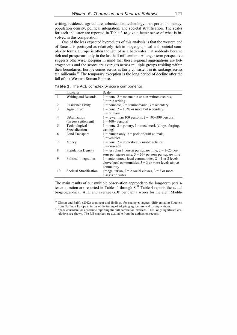
William R. Thompson and Kentaro Sakuwa 121
writing, residence, agriculture, urbanization, technology, transportation, money, population density, political integration, and societal stratification. The scales for each indicator are reported in Table 3 to give a better sense of what is in-volved in this computation.
One of the less expected byproducts of this analysis is that the western end of Eurasia is portrayed as relatively rich in biogeographical and societal com-plexity terms. Europe is often thought of as a backwater that suddenly became rich and prosperous only in the last half millennium. A longer term perspective suggests otherwise. Keeping in mind that these regional aggregations are het-erogeneous and the scores are averages across multiple groups residing within their boundaries, Europe comes across as fairly consistent in its rankings across ten millennia.30 The temporary exception is the long period of decline after the fall of the Western Roman Empire.
Table 3. The ACE complexity score components
Indicator Scale 1 Writing and Records 1 = none, 2 = mnemonic or non-written records,
3 = true writing 2 Residence Fixity 1 = nomadic, 2 = seminomadic, 3 = sedentary 3 Agriculture 1 = none, 2 = 10 % or more but secondary,
3 = primary 4 Urbanization
(largest settlement) 1 = fewer than 100 persons, 2 = 100–399 persons, 3 = 400+ persons
5 Technological Specialization
1 = none, 2 = pottery, 3 = metalwork (alloys, forging, casting)
6 Land Transport 1 = human only, 2 = pack or draft animals, 3 = vehicles
7 Money 1 = none, 2 = domestically usable articles, 3 = currency
8 Population Density 1 = less than 1 person per square mile, 2 = 1–25 per-sons per square mile, 3 = 26+ persons per square mile
9 Political Integration 1 = autonomous local communities, 2 = 1 or 2 levels above local communities, 3 = 3 or more levels above community
10 Societal Stratification 1= egalitarian, 2 = 2 social classes, 3 = 3 or more classes or castes
The main results of our multiple observation approach to the long-term persis-tence question are reported in Tables 4 through 8.31 Table 4 reports the actual biogeographical, ACE and average GDP per capita scores for the eight Maddi-
30 Olsson and Paik's (2012) argument and findings, for example, suggest differentiating Southern
from Northern Europe in terms of the timing of adopting agriculture and its implications. 31 Space considerations preclude reporting the full correlation matrices. Thus, only significant cor-
relations are shown. The full matrices are available from the authors on request.
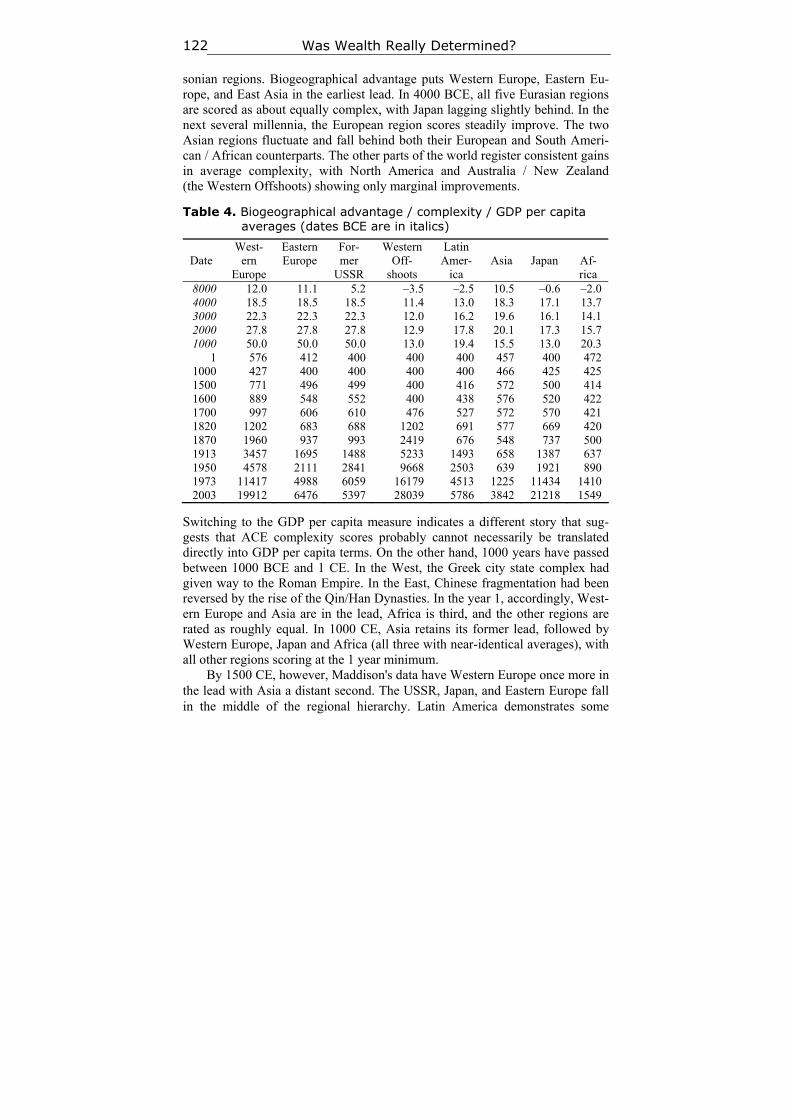
Was Wealth Really Determined? 122
sonian regions. Biogeographical advantage puts Western Europe, Eastern Eu-rope, and East Asia in the earliest lead. In 4000 BCE, all five Eurasian regions are scored as about equally complex, with Japan lagging slightly behind. In the next several millennia, the European region scores steadily improve. The two Asian regions fluctuate and fall behind both their European and South Ameri-can / African counterparts. The other parts of the world register consistent gains in average complexity, with North America and Australia / New Zealand (the Western Offshoots) showing only marginal improvements.
Table 4. Biogeographical advantage / complexity / GDP per capita averages (dates BCE are in italics)
Date
West-ern
Europe
Eastern Europe
For-mer
USSR
Western Off-
shoots
Latin Amer-
ica
Asia
Japan
Af-rica
8000 12.0 11.1 5.2 –3.5 –2.5 10.5 –0.6 –2.0 4000 18.5 18.5 18.5 11.4 13.0 18.3 17.1 13.7 3000 22.3 22.3 22.3 12.0 16.2 19.6 16.1 14.1 2000 27.8 27.8 27.8 12.9 17.8 20.1 17.3 15.7 1000 50.0 50.0 50.0 13.0 19.4 15.5 13.0 20.3
1 576 412 400 400 400 457 400 472 1000 427 400 400 400 400 466 425 425 1500 771 496 499 400 416 572 500 414 1600 889 548 552 400 438 576 520 422 1700 997 606 610 476 527 572 570 421 1820 1202 683 688 1202 691 577 669 420 1870 1960 937 993 2419 676 548 737 500 1913 3457 1695 1488 5233 1493 658 1387 637 1950 4578 2111 2841 9668 2503 639 1921 890 1973 11417 4988 6059 16179 4513 1225 11434 1410 2003 19912 6476 5397 28039 5786 3842 21218 1549
Switching to the GDP per capita measure indicates a different story that sug-gests that ACE complexity scores probably cannot necessarily be translated directly into GDP per capita terms. On the other hand, 1000 years have passed between 1000 BCE and 1 CE. In the West, the Greek city state complex had given way to the Roman Empire. In the East, Chinese fragmentation had been reversed by the rise of the Qin/Han Dynasties. In the year 1, accordingly, West-ern Europe and Asia are in the lead, Africa is third, and the other regions are rated as roughly equal. In 1000 CE, Asia retains its former lead, followed by Western Europe, Japan and Africa (all three with near-identical averages), with all other regions scoring at the 1 year minimum.
By 1500 CE, however, Maddison's data have Western Europe once more in the lead with Asia a distant second. The USSR, Japan, and Eastern Europe fall in the middle of the regional hierarchy. Latin America demonstrates some
William R. Thompson and Kentaro Sakuwa 123
slight gain while Africa manifests steady decline. North America and Austra-lia's position and wealth/technology level is shown as remaining unchanged for 1500 years. Then the scores change dramatically. The western European GDP per capita almost doubles by 1820. The Western Offshoots (North America and Australia / New Zealand) are not far behind. Eastern Europe, the USSR, and Latin America have made some progress with development levels that are about half those of the leaders. Average 1820 Asian and African GDP per cap-ita are little changed from their 1500 levels. By the end of the 20th century, the Western Offshoots, Western Europe, and Japan have created strong leads. Latin America and the USSR are in the middle of the hierarchy but considerably be-hind the leaders. Eastern Europe, Asia, and Africa occupy the bottom of the regional hierarchy.
Table 5 reports the same data in regional rank order. The long-term out-come encompasses several significant shifts in relative standing. Western Eu-rope is an early leader but falters in the Medieval Era before rising to the lead after the industrial revolution – a lead it does not maintain beyond the 19th cen-tury. The Western Offshoots remain in the technology/growth cellar throughout most of the ten millennia period studied before seizing the lead in the last cen-tury. Asia begins in the middle, rises to the lead in the first millennium CE, and then falls back toward the bottom. Japan's position oscillates – initially middle, then falling back to low, then to high, back to the middle, and then back to high. Eastern Europe and the USSR begin relatively high and decline to the middle. Latin America starts low and never exceeds a middle ranking. Africa tends to stay near the bottom except in the first millennium CE.
Scanning rank orders is one thing. We can improve on this form of data in-spection by calculating Spearman Rank Order coefficients from observation to observation, as is done in Tables 6 and 7. Table 6 reports significant coeffi-cients without any modification of the rank orders. Table 7 corrects for the more recent European migrations, following a technique utilized by Comin et al. (2010).32 In Table 6, there are basically four clusters of coefficients.
32 Comin et al. (2010) utilize Putterman and Weil's (2009) matrix on post-1500 migrations to cor-
rect 1500 and onward outcomes by the proportion of national population that has migrated into the country. We do the same for regional aggregations. Putterman and Weil's original migration matrix includes information of the migration from 1500 to 2000 for 165 countries. This state-level matrix was converted to a regional-level matrix, so that the modified matrix gives the pro-portions of each region's population in the year of 2000 that resided in its own and other regions in 1500. As in Comin et al., pre-1500 regional rankings were generated by pre-multiplying the ‘raw’ vectors of wealth/technology scores by the modified (regional) migration matrix. The re-sulting historical rankings thus reflect the post-1500 migration on the regional basis. For details of the migration matrix, see Putterman and Weil (2009, 2010).

Was Wealth Really Determined? 124
Table 5. Regional rank orders
Date West-
ern Europe
Eastern Europe
For-mer
USSR
Western Off-
shoots
Latin Amer-
ica Asia
Ja-pan
Af-rica
8000 2 1 4 8 7 3 5 6 4000 1 1 1 8 7 4 5 6 3000 1 1 1 8 5 4 6 7 2000 1 1 1 8 5 4 6 7 1000 1 1 1 7 5 6 7 4
1 1 4 5 5 5 3 5 2 1000 2 4 4 4 4 1 3 3 1500 1 5 4 8 6 2 3 7 1600 1 4 3 8 6 2 5 7 1700 1 3 2 7 6 4 5 8 1820 1 5 4 1 3 7 6 8 1870 2 4 3 1 6 7 5 8 1913 2 3 5 1 4 7 6 8 1950 2 5 3 1 4 8 6 7 1973 3 5 4 1 6 8 2 7 2003 3 4 6 1 5 7 2 8
Table 6. Significant Spearman rank order coefficients (only entries with P < 0.05 are shown; column numbers correspond to row numbers)
Date 1 2 3 4 – 8 9 – 11 12 13 14 15 8000 1 4000 2 .93 3000 3 .85 .93 2000 4 .85 .93 1.0 1000 5 .77 .81 .81
1 6 1000 7 1500 8 .71 1600 9 .85 .85 .85 .93 1700 10 .90 .93 .93 .79 .91 1820 11 1870 12 .85 1913 13 .92 .88 1950 14 .95 .91 .88 1973 15 .83 .74 2003 16 .76 .76 .91
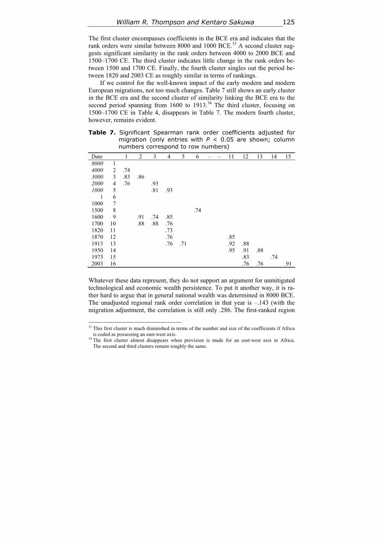
William R. Thompson and Kentaro Sakuwa 125
The first cluster encompasses coefficients in the BCE era and indicates that the rank orders were similar between 8000 and 1000 BCE.33 A second cluster sug-gests significant similarity in the rank orders between 4000 to 2000 BCE and 1500–1700 CE. The third cluster indicates little change in the rank orders be-tween 1500 and 1700 CE. Finally, the fourth cluster singles out the period be-tween 1820 and 2003 CE as roughly similar in terms of rankings.
If we control for the well-known impact of the early modern and modern European migrations, not too much changes. Table 7 still shows an early cluster in the BCE era and the second cluster of similarity linking the BCE era to the second period spanning from 1600 to 1913.34 The third cluster, focusing on 1500–1700 CE in Table 4, disappears in Table 7. The modern fourth cluster, however, remains evident.
Table 7. Significant Spearman rank order coefficients adjusted for migration (only entries with P < 0.05 are shown; column numbers correspond to row numbers)
Date 1 2 3 4 5 6 – – 11 12 13 14 15 8000 1 4000 2 .74 3000 3 .83 .86 2000 4 .76 .93 1000 5 .81 .93
1 6 1000 7 1500 8 .74 1600 9 .91 .74 .85 1700 10 .88 .88 .76 1820 11 .73 1870 12 .76 .85 1913 13 .76 .71 .92 .88 1950 14 .95 .91 .88 1973 15 .83 .74 2003 16 .76 .76 .91
Whatever these data represent, they do not support an argument for unmitigated technological and economic wealth persistence. To put it another way, it is ra-ther hard to argue that in general national wealth was determined in 8000 BCE. The unadjusted regional rank order correlation in that year is –.143 (with the migration adjustment, the correlation is still only .286. The first-ranked region
33 This first cluster is much diminished in terms of the number and size of the coefficients if Africa
is coded as possessing an east-west axis. 34 The first cluster almost disappears when provision is made for an east-west axis in Africa.
The second and third clusters remain roughly the same.
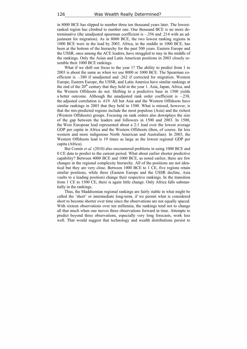
Was Wealth Really Determined? 126
in 8000 BCE has slipped to number three ten thousand years later. The lowest-ranked region has climbed to number one. One thousand BCE is no more de-terminative (the unadjusted spearman coefficient is –.356 and .214 with an ad-justment for migration). As in 8000 BCE, the two lowest ranking regions in 1000 BCE were in the lead by 2003. Africa, in the middle in 1000 BCE, has been at the bottom of the hierarchy for the past 500 years. Eastern Europe and the USSR, once among the ACE leaders, have struggled to stay in the middle of the rankings. Only the Asian and Latin American positions in 2003 closely re-semble their 1000 BCE rankings.
What if we shift our focus to the year 1? The ability to predict from 1 to 2003 is about the same as when we use 8000 or 1000 BCE. The Spearman co-efficient is –.380 if unadjusted and .262 if corrected for migration. Western Europe, Eastern Europe, the USSR, and Latin America have similar rankings at the end of the 20th century that they held in the year 1. Asia, Japan, Africa, and the Western Offshoots do not. Shifting to a predictive base in 1500 yields a better outcome. Although the unadjusted rank order coefficient is –.238, the adjusted correlation is .619. All but Asia and the Western Offshoots have similar rankings in 2003 that they held in 1500. What is missed, however, is that the mis-predicted regions include the most populous (Asia) and the richest (Western Offshoots) groups. Focusing on rank orders also downplays the size of the gap between the leaders and followers in 1500 and 2003. In 1500, the West European lead represented about a 2:1 lead over the lowest average GDP per capita in Africa and the Western Offshoots (then, of course, far less western and more indigenous North American and Australian). In 2003, the Western Offshoots lead is 19 times as large as the lowest regional GDP per capita (Africa).
But Comin et al. (2010) also encountered problems in using 1000 BCE and 0 CE data to predict to the current period. What about earlier shorter predictive capability? Between 4000 BCE and 1000 BCE, as noted earlier, there are few changes in the regional complexity hierarchy. All of the positions are not iden-tical but they are very close. Between 1000 BCE to 1 CE, five regions retain similar positions, while three (Eastern Europe and the USSR decline, Asia vaults to a leading position) change their respective rankings. In the transition from 1 CE to 1500 CE, there is again little change. Only Africa falls substan-tially in the rankings.
Thus, the Maddisonian regional rankings are fairly stable in what might be called the ‘short’ or intermediate long-term, if we permit what is considered short to become shorter over time since the observations are not equally spaced. With sixteen observations over ten millennia, the rankings tend not to change all that much when one moves three observations forward in time. Attempts to predict beyond three observations, especially very long forecasts, work less well. That would suggest that technology and wealth distributions persist to
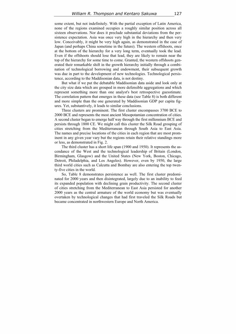
William R. Thompson and Kentaro Sakuwa 127
some extent, but not indefinitely. With the partial exception of Latin America, none of the regions examined occupies a roughly similar position across all sixteen observations. Nor does it preclude substantial deviations from the per-sistence expectation. Asia was once very high in the hierarchy and then very low. Conceivably, it might be very high again, as demonstrated in the case of Japan (and perhaps China sometime in the future). The western offshoots, once at the bottom of the hierarchy for a very long term, eventually took the lead. Even if the offshoots should lose that lead, they are likely to remain near the top of the hierarchy for some time to come. Granted, the western offshoots gen-erated their remarkable shift in the growth hierarchy initially through a combi-nation of technological borrowing and endowment, their subsequent growth was due in part to the development of new technologies. Technological persis-tence, according to the Maddisonian data, is not destiny.
But what if we put the debatable Maddisonian data aside and look only at the city size data which are grouped in more defensible aggregations and which represent something more than one analyst's best retrospective guesstimate. The correlation pattern that emerges in these data (see Table 8) is both different and more simple than the one generated by Maddisonian GDP per capita fig-ures. Yet, substantively, it leads to similar conclusions.
Three clusters are prominent. The first cluster encompasses 3700 BCE to 2000 BCE and represents the most ancient Mesopotamian concentration of cities. A second cluster began to emerge half way through the first millennium BCE and persists through 1800 CE. We might call this cluster the Silk Road grouping of cities stretching from the Mediterranean through South Asia to East Asia. The names and precise locations of the cities in each region that are most prom-inent in any given year vary but the regions retain their relative standings more or less, as demonstrated in Fig. 2.
The third cluster has a short life span (1900 and 1950). It represents the as-cendance of the West and the technological leadership of Britain (London, Birmingham, Glasgow) and the United States (New York, Boston, Chicago, Detroit, Philadelphia, and Los Angeles). However, even by 1950, the large third world cities such as Calcutta and Bombay are also entering the top twen-ty-five cities in the world.
So, Table 8 demonstrates persistence as well. The first cluster predomi-nated for 2000 years and then disintegrated, largely due to an inability to feed its expanded population with declining grain productivity. The second cluster of cities stretching from the Mediterranean to East Asia persisted for another 2000 years as the central armature of the world economy but was eventually overtaken by technological changes that had first traveled the Silk Roads but became concentrated in northwestern Europe and North America.
Was Wealth Really Determined? 128
Table 8. City size correlations across time
Note: Only entries with P < 0.05 are shown. Pairwise, year-to-year, correlation coeffi-cients are obtained based on the analysis of each region's share of city population. Years BCE in italics.
Fig. 2. Northern Mediterranean / West European and East Asian
regional city share scores
The third cluster seems unlikely to retain its prominence for another 2000 years. If nothing else, city size is no longer a reliable instrument for capturing wealth and technological leadership as it once was. But the diffusion of wealth and technology is taking place faster than it once did (Comin and Hobijn 2010). The persistence of relative regional standings, as a consequence, must also be expected to change to varying extents as some once low ranking areas rise in the rankings. Yet there is also no reason to assume that all low-ranking regions
William R. Thompson and Kentaro Sakuwa 129
will rise equally. In that respect, some mixture of persistence and change should be anticipated.
Since the patterns that emerge vary by indicator, do we need to pick and choose which one seems to have the greatest validity? The city size data dem-onstrate what we earlier described as largely missing from the earlier analyses of Olsson and Hibbs (2005) and Comin, Easterly, and Gong (2010). The city data isolate the Sumerian starting point for relatively large cities and underscore the ‘dumb-bell’ interaction between the Mediterranean and East Asia across Diamond's east-west axis. They also capture the post-1800 shift in cities due to industrialization. In these respects, the city size data most clearly conform to our understanding of the major shifts in, and evolution of, world history. Yet as long as all our indicators underline the limitations of persistence, there is really no reason to focus on one index alone. Multiple indicators show roughly similar mixtures of persistence and abrupt change.
Conclusion
Our point throughout has been that there are important limitations on path de-pendencies in historical economic growth patterns. Diamond's argument about east-west axis and the number of plants and large mammals certainly helps ex-plain Eurasia's advantages over Africa and the Americas. It does not tell us too much about what happened within Eurasia after the creation of the world's con-tinents. Whether we use biogeographical, societal complexity, GDP per capita, or city size indicators, there are very clear limits on the ability to predict in the long term who will be ahead in one year. Some places have been advantaged over others but not to the extent of predetermining economic growth well into the future. We cannot predict who precisely within Eurasia will get ahead based on Eurasia's initial advantage. Nor could we have predicted how long any Eura-sian advantage might persist, except to say that it did not last forever. Using our indicators, we cannot predict who will be on ‘first base’ in 1 CE based on in-formation in 1000 BCE. We cannot predict who will be ahead in 1950 or 1998 based on information in 1500. These prediction failures are not based on vola-tility in the data. There is substantial persistence across selected intervals. But there are also substantial shifts due ostensibly to leads and lags in technological leadership, demographic differentials, migration, climate change, disease, and warfare.
If we grant that human existence on planet Earth is characterized by some tendencies toward the stickiness of wealth and technological persistence subject to strong temporal limitations, the most interesting questions involve why these persistence tendencies fail to bar very substantial changes in regional and na-tional rankings in economic wealth. We probably understand the reasons for technological and wealth persistence best. We do less well explaining how these characteristics are overwhelmed or in predicting how they may change in
Was Wealth Really Determined? 130
the future. It is conceivable, but by no means guaranteed, that an emphasis on very long-term shifts in technology and wealth will give us a better perspective on why the rich do not always get richer (or even stay rich) and why the poor sometimes improve their standings in the world pecking order.
References
Acemoglu D., and Johnson S. 2012. Why Nations Fail: The Origins of Power, Pros-perity and Poverty. New York: Crown.
Acemoglu D., Johnson S., and Robinson J. A. 2001. The Colonial Origins of Com-parative Development: An Empirical Investigation. American Economic Review 91: 1369–1401.
Acemoglu D., Johnson S., and Robinson J. A. 2002. Reversal of Fortune: Geography and Institutions in the Making of the Modern World Income Distribution. Quarterly Journal of Economics 117: 1231–1294.
Archer C. I., Ferris J. R., Herwig H. H., and Travers T. H. E. 2002. World History of Warfare. Lincoln, NE: University of Nebraska Press.
Bleaney M., and Dimico A. 2011. Biogeographical Conditions, the Transition to Agri-culture, and Long-Run Growth. European Economic Review 55 (7): 943–954.
Burroughs W. J. 2005. Climate Change in Prehistory: The End of the Reign of Chaos. Cambridge: Cambridge University Press.
Chanda A., and Putterman L. 2005. State Effectiveness, Economic Growth, and the Age of States. States and Development: Historical Antecedents of Stagnation and Advance / Ed. by M. Lange, and D. Rueschemeyer, pp. 69–91. London: Palgrave Macmillan.
Chanda A., and Putterman L. 2007. Early States, Reversals and Catch-up in the Proc-ess of Economic Development. Scandinavian Journal of Economics 109: 387–413.
Chandler T. 1987. Four Thousand Years of Urban Growth: An Historical Census. Lewiston, NY – Queenston: St. David's University Press.
Chase-Dunn C., and Willard A. 1994. Cities in the Central Political-Military Network since CE 1200. Comparative Civilizations Review 30: 104–132.
Chase-Dunn C., Manning S., and Hall T. D. 2000. Rise and Fall: East-West Synchro-nicity and Indic Exceptionalism Reexamined. Social Science History 24(4): 721–748.
Chase-Dunn C., and Manning S. 2002. City Systems and World Systems: Four Mil-lennia of City Growth and Decline. Cross-Cultural Research 36(4): 379–398.
Chase-Dunn C., Hall T., and Turchin P. 2007. World-Systems in the Biogeosphere: Urbanized State Formation, and Climate Change since the Iron Age. The World Sys-tem and the Earth System: Global Socioenvironmental Change and Sustainability Since the Neolithic / Ed. by A. Hornbrog, and C. C. Crumley, pp. 132–148. Walnut Creek, CA: Left Coast Books.
Clark G. 2007. A Farewell to Alms: A Brief Economic History of the World. Princeton, NJ: Princeton University Press.
William R. Thompson and Kentaro Sakuwa 131
Comin D., Easterly W., and Gong E. 2010. Was the Wealth of Nations Determined in 1000 BC? American Economic Journal: Macroeconomics 2: 65–97.
Comin D., and Hobijn B. 2010. An Exploration of Technology Diffusion. American Economic Review 100: 2031–2059.
Diamond J. 1997. Guns, Germs and Steel: The Fate of Human Societies. New York: W.W. Norton.
Duijn J. J. van 1983. The Long Wave in Economic Life. London: George Allen and Unwin.
Findlay R., and O'Rourke K. H. 2007. Power and Plenty: Trade, War and the World Economy in the Second Millennium. Princeton, NJ: Princeton University Press.
Frachetti M. D., Spengler R. N., Fritz G. J., and Mar'yashev A. N. 2010. Earliest Direct Evidence for Broomcorn Millet and Wheat in the Central Eurasian Steppe Region. Antiquity 84: 993–1010.
Frank A. G. 1998. ReOrient: Global Economy in the Asian Age. Berkeley, CA: Univer-sity of California Press.
Galor O. 2011. Unified Growth Theory. Princeton, NJ: Princeton University Press.
Hogg I., and Batchelor J. 1978. Naval Gun. Poole: Blandford Press.
Imamura K. 1996. Jomon and Yayoi: The Transition to Agriculture in Japanese Prehis-tory. The Origins and Spread of Agriculture and Pastoralism in Eurasia / Ed. by D. R. Harris, pp. 442–464. Washington: Smithsonian Institution Press.
Krieckhaus J. 2006. Dictating Development: How Europe Shaped the Global Periph-ery. Pittsburgh, PA: University of Pittsburgh Press.
Landes D. S. 1998. The Wealth and Poverty of Nations: Why Some Are So Rich and Some Are So Poor. New York: W.W. Norton.
Maddison A. 1995. Monitoring the World Economy, 1820–1992. Paris: OECD.
Maddison A. 2001. The World Economy: A Millennial Perspective. Paris: OECD.
Maddison A. 2007. Contours of the World Economy, 1–2030 AD: Essays in Macro-Economic History. Oxford: Oxford University Press.
Modelski G. 2003. World Cities: –3000 to 2000. Washington: Faros 2000.
Modelski G., and Thompson W. R. 1988. Sea Power in Global Politics, 1494–1993. London: Macmillan.
Modelski G., and Thompson W. R. 1996. Leading Sectors and World Powers: The Coevolution of Global Politics and Economics. Columbia, SC: University of South Carolina Press.
Morris I. 2010. Why the West Rules – For Now: The Patterns of History, and What They Reveal about the Future. New York: Farrar, Straus and Giroux.
Morris I. 2013. The Measure of Civilization: How Social Development Decides the Fate of Nations. Princeton, NJ: Princeton University Press.
Olsson O., and Hibbs D. A. Jr. 2005. Biogeography and Long-Run Economic Devel-opment. European Economic Review 49: 909–938.
Was Wealth Really Determined? 132
Olsson O., and Paik C. 2013. A Western Reversal since the Neolithic? The Long-Run Impact of Early Agriculture. Working Papers in Economics 552, University of Gothenburg, Department of Economics. URL: https://gupea.ub.gu.se/bitstream/ 2077/32052/1/gupea_2077_32052.1.pdf.
Parker G. 1988. The Military Revolution: Military Innovation and the Rise of the West, 1500–1800. Cambridge: Cambridge University Press.
Parthasarathi P. 2011. Why Europe Grew Rich and Asia Did Not: Global Economic Divergence, 1600–1850. Cambridge: Cambridge University Press.
Peregrine P. N. 2003. Atlas of Cultural Evolution. World Cultures 14(1): 1–75.
Peregrine P. N., and Embers M. (Eds.) 2001. Encyclopedia of Prehistory. 9 vols. New York: Kluwer Academic/Plenum Publishers.
Pomeranz K. 2000. The Great Divergence: China, Europe and the Making of the Mod-ern World Economy. Princeton, NJ: Princeton University Press.
Putterman L. 2008. Agriculture, Diffusion and Development: Ripple Effects of the Neolithic Revolution. Economica 75: 729–748.
Putterman L., and Weil D. 2009. Main Appendix to World Migration Matrix, 1500–2000, version 1.1. Brown University Department of Economics. URL: http://www. econ.brown.edu/fac/louis_putterman/world%20migration%20matrix.htm.
Putterman L., and Weil D. 2010. Post-1500 Population Flows and the Long Run De-terminants of Economic Growth and Inequality. The Quarterly Journal of Econom-ics 125(4): 1627–1682.
Rosenthal J.-L., and Wong R. B. 2011. Before and Beyond Divergence: The Politics of Economic Change in China and Europe. Cambridge, MA: Harvard University Press.
Sachs J., Mellinger A. D., and Gallup J. L. 2001. The Geography of Poverty and Wealth. Scientific American 284(3): 71–75.
Singer J. D., Bremer S., and Stuckey J. 2010 [1972]. Capability Distribution, Uncer-tainty, and Major Power War, 1820–1965. Peace, War, and Numbers / Ed. by B. Russett, pp. 19–48. Beverly Hills, CA: Sage.
Smith B. D. 1995. The Emergence of Agriculture. New York: Scientific American Li-brary.
Thomas J. 1996. The Cultural Context of the First Use of Domesticates in Continental Central and Northwest Europe. The Origins and Spread of Agriculture and Pastoral-ism in Eurasia / Ed. by D. R. Harris, pp. 310–322. Washington: Smithsonian Institu-tion Press.
Thompson W. R. 1999. The Military Superiority Thesis and the Ascendancy of West-ern Eurasia in the World System. Journal of World History 10: 143–178.
Turchin P., Adams J. M., and Hall T. D. 2006. East-West Orientation of Historical Empires and Modern States. Journal of World-Systems Research 12(2): 218–229.
Wong R. B. 1997. China Transformed: Historical Change and the Limits of European Experience. Ithaca, NY: Cornell University Press.
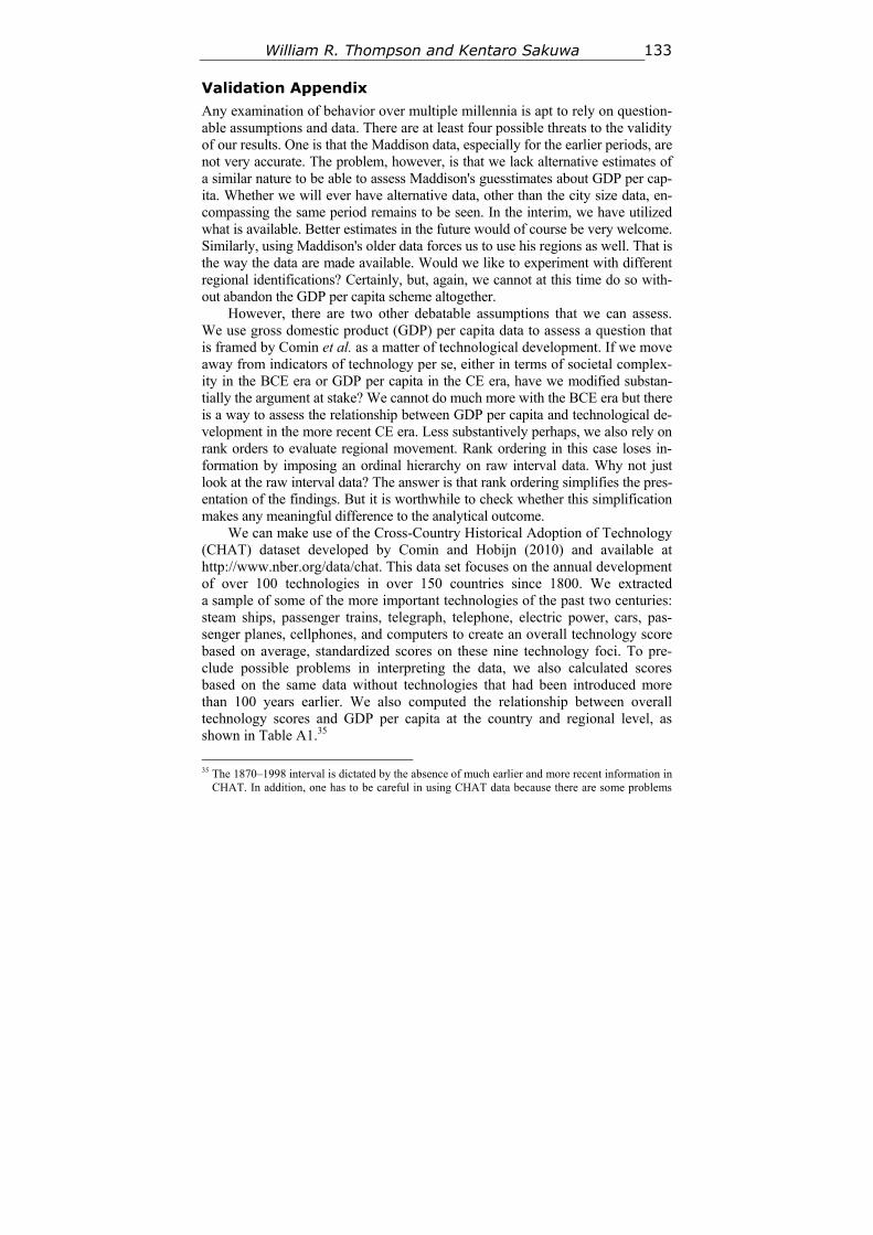
William R. Thompson and Kentaro Sakuwa 133
Validation Appendix
Any examination of behavior over multiple millennia is apt to rely on question-able assumptions and data. There are at least four possible threats to the validity of our results. One is that the Maddison data, especially for the earlier periods, are not very accurate. The problem, however, is that we lack alternative estimates of a similar nature to be able to assess Maddison's guesstimates about GDP per cap-ita. Whether we will ever have alternative data, other than the city size data, en-compassing the same period remains to be seen. In the interim, we have utilized what is available. Better estimates in the future would of course be very welcome. Similarly, using Maddison's older data forces us to use his regions as well. That is the way the data are made available. Would we like to experiment with different regional identifications? Certainly, but, again, we cannot at this time do so with-out abandon the GDP per capita scheme altogether.
However, there are two other debatable assumptions that we can assess. We use gross domestic product (GDP) per capita data to assess a question that is framed by Comin et al. as a matter of technological development. If we move away from indicators of technology per se, either in terms of societal complex-ity in the BCE era or GDP per capita in the CE era, have we modified substan-tially the argument at stake? We cannot do much more with the BCE era but there is a way to assess the relationship between GDP per capita and technological de-velopment in the more recent CE era. Less substantively perhaps, we also rely on rank orders to evaluate regional movement. Rank ordering in this case loses in-formation by imposing an ordinal hierarchy on raw interval data. Why not just look at the raw interval data? The answer is that rank ordering simplifies the pres-entation of the findings. But it is worthwhile to check whether this simplification makes any meaningful difference to the analytical outcome.
We can make use of the Cross-Country Historical Adoption of Technology (CHAT) dataset developed by Comin and Hobijn (2010) and available at http://www.nber.org/data/chat. This data set focuses on the annual development of over 100 technologies in over 150 countries since 1800. We extracted a sample of some of the more important technologies of the past two centuries: steam ships, passenger trains, telegraph, telephone, electric power, cars, pas-senger planes, cellphones, and computers to create an overall technology score based on average, standardized scores on these nine technology foci. To pre-clude possible problems in interpreting the data, we also calculated scores based on the same data without technologies that had been introduced more than 100 years earlier. We also computed the relationship between overall technology scores and GDP per capita at the country and regional level, as shown in Table A1.35
35 The 1870–1998 interval is dictated by the absence of much earlier and more recent information in
CHAT. In addition, one has to be careful in using CHAT data because there are some problems
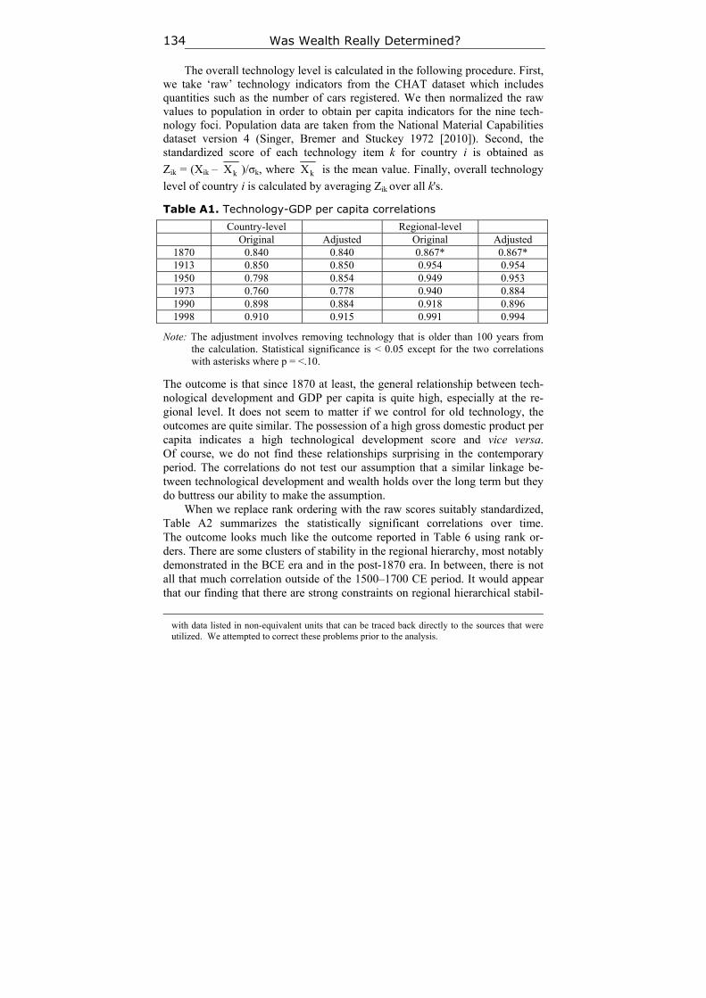
Was Wealth Really Determined? 134
The overall technology level is calculated in the following procedure. First, we take ‘raw’ technology indicators from the CHAT dataset which includes quantities such as the number of cars registered. We then normalized the raw values to population in order to obtain per capita indicators for the nine tech-nology foci. Population data are taken from the National Material Capabilities dataset version 4 (Singer, Bremer and Stuckey 1972 [2010]). Second, the standardized score of each technology item k for country i is obtained as
Zik = (Xik – kX )/σk, where kX is the mean value. Finally, overall technology
level of country i is calculated by averaging Zik over all k's.
Table A1. Technology-GDP per capita correlations
Country-level Regional-level Original Adjusted Original Adjusted
1870 0.840 0.840 0.867* 0.867* 1913 0.850 0.850 0.954 0.954 1950 0.798 0.854 0.949 0.953 1973 0.760 0.778 0.940 0.884 1990 0.898 0.884 0.918 0.896 1998 0.910 0.915 0.991 0.994
Note: The adjustment involves removing technology that is older than 100 years from the calculation. Statistical significance is < 0.05 except for the two correlations with asterisks where p = <.10.
The outcome is that since 1870 at least, the general relationship between tech-nological development and GDP per capita is quite high, especially at the re-gional level. It does not seem to matter if we control for old technology, the outcomes are quite similar. The possession of a high gross domestic product per capita indicates a high technological development score and vice versa. Of course, we do not find these relationships surprising in the contemporary period. The correlations do not test our assumption that a similar linkage be-tween technological development and wealth holds over the long term but they do buttress our ability to make the assumption.
When we replace rank ordering with the raw scores suitably standardized, Table A2 summarizes the statistically significant correlations over time. The outcome looks much like the outcome reported in Table 6 using rank or-ders. There are some clusters of stability in the regional hierarchy, most notably demonstrated in the BCE era and in the post-1870 era. In between, there is not all that much correlation outside of the 1500–1700 CE period. It would appear that our finding that there are strong constraints on regional hierarchical stabil-
with data listed in non-equivalent units that can be traced back directly to the sources that were utilized. We attempted to correct these problems prior to the analysis.

William R. Thompson and Kentaro Sakuwa 135
ity in the really long term is not due to using rank ordered data. Similar out-comes emerge from the raw data as well.
Table A2. Regional hierarchy correlations over time with adjustment –8
0 0 0
–4 0 0 0
–3 0 0 0
–2 0 0 0
–1 0 0 0
1 1 0 0 0
1 5 0 0
1 6 0 0
1 7 0 0
1 8 0 0
1 8 2 0
1 8 7 0
1 9 1 3
1 9 5 0
1 9 7 3
–8000 –4000 .853 –3000 .888 .903 –2000 .835 .835 .977 –1000 .695 .636 .849 .941
1 1000 1500 .743 .815 .989 1600 .741 .718 .707 .804 .947 .978 1700 .744 1800 1820 1870 .964 1913 .941 .984 1950 .875 .943 .980 1973 .845 .847 .873 .851 2003 .818 .811 .835 .796 .976
Note: Only correlations significant at the < .05 level are reported.
History & Mathematics: Trends and Cycles 2014 136–158
136
II. CYCLICAL PROCESSES IN PRE-INDUSTRIAL SOCIETIES
4
Cycling in the Complexity of Early Societies
Sergey Gavrilets, David G. Anderson,
and Peter Turchin
Abstract
Warfare is commonly viewed as a driving force of the process of aggregation of initially independent villages into larger and more complex political units that started several thousand years ago and quickly led to the appearance of chief-doms, states, and empires. Here we build on extensions and generalizations of Carneiro's (1970) argument to develop a spatially explicit agent-based model of the emergence of early complex societies via warfare. In our model polities are represented as hierarchically structured networks of villages whose size, power, and complexity change as a result of conquest, secession, internal reor-ganization (via promotion and linearization), and resource dynamics. A general prediction of our model is continuous stochastic cycling in which the growth of individual polities in size, wealth/power, and complexity is inter-rupted by their quick collapse. The model dynamics are mostly controlled by two parameters, one of which scales the relative advantage of wealthier polities in between- and within-polity conflicts, and the other is the chief's expected time in power. Our results demonstrate that the stability of large and complex polities is strongly promoted if the outcomes of the conflicts are mostly deter-mined by the polities' wealth/power, if there exist well-defined and accepted means of succession, and if control mechanisms are internally specialized.
Keywords: modeling, warfare, state, territory, rebellion.
Introduction
For most of humanity's existence people lived in small egalitarian bands or vil-lages that were politically autonomous. However, a qualitative change hap-pened roughly 10,000 years ago when villages began aggregating into larger and more complex, hierarchically-structured polities (a general term that in-cludes not only states and empires but also smaller-scale independent political
Sergey Gavrilets, David G. Anderson, and Peter Turchin 137
units, such as chiefdoms, acephalous tribes, and autonomous villages, see, e.g., Ferguson and Mansbach 1996). This process of aggregation first took place in Mesopotamia, East Asia, South America, and Mesoamerica, followed by sec-ondary developments elsewhere (Service 1975). The process of aggregation led, over time, to the emergence of chiefdoms, states, and empires. Once estab-lished, these complex societies rose and fell over time, with centers of power and authority shifting from one location to another over the landscape, a proc-ess that has been described as cycling (Wright 1977, 1984; Cordy 1981; Kirch 1984; Marcus 1992, 1998; Anderson 1994, 1996; Earle 1997; Cioffi-Revilla and Landman 1999; Junker 1999; Hall 2001). The causes of this process have fascinated scholars and been the subject of speculation for centuries (Engels 1884; Lenin 1918; Childe 1950; Wittfogel 1957; Adams 1966; Fried 1967; Flannery 1972; Webster 1975; Wright 1977, 1984, 1986; Service 1975, 1978; Ferguson and Mansbach 1996; Earle 1997; Trigger 2003; Cioffi-Revilla 2005; Drennan and Peterson 2006; Turchin and Gavrilets 2009; Spencer 2010).
Here we are concerned with a set of influential theories that put special emphasis on warfare between different polities (starting with villages). When warfare first occurred in human (pre)history is controversial, although it is as-sumed to have been relatively small in scale and consequence until complex and presumably multicommunity societies emerged (Ferguson 1984; Haas 2004; Trigger 2003; but see Keeley 1997; Cioffi-Revilla 2000). Besides war-fare, there are of course a number of additional prerequisites for the evolution of social complexity. One requirement, emphasized by Carneiro, is circum-scription (environmental, due to the resource concentration, or social, due to the presence of other human groups nearby; see Carneiro 1970, 1981). Circum-scription was the factor that precluded losing communities from moving away and thus separating themselves spatially and politically from victors. Other pre-requisites include existence of agricultural potential capable of generating sur-pluses and significant variation in productive and/or demographic potential among local communities (Webster 1975). Equally important was ability to delegate power and the invention of hierarchically structured control mecha-nisms in which each superior directly controlled only a limited number of sub-ordinates (Flannery 1972; Wright 1977, 1984; Turchin and Gavrilets 2009). The latter was also important for the subsequent growth of polities given what has been called ‘scalar stress’, a decrease in the ability of leaders to process information and maintain efficient control over subordinates as their number (herein, the number of subordinate villages) increased (Johnson 1982). The outcome of these processes and factors was the emergence of simple chief-doms (Steponaitis 1978, 1981; Wright 1984) in which one village controlled (and received tribute from) several subordinate villages. More complex polities were characterized by greater numbers of subordinate levels, with complex chiefdoms, paramount chiefdoms, and state societies typically defined as those
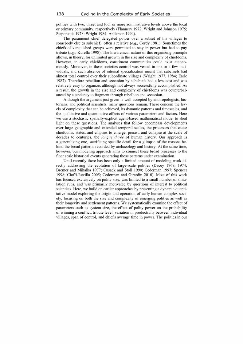
Cycling in the Complexity of Early Societies 138
polities with two, three, and four or more administrative levels above the local or primary community, respectively (Flannery 1972; Wright and Johnson 1975; Steponaitis 1978; Wright 1984; Anderson 1994).
The paramount chief delegated power over a subset of his villages to somebody else (a subchief), often a relative (e.g., Cordy 1981). Sometimes the chiefs of vanquished groups were permitted to stay in power but had to pay tribute (e.g., Kurella 1998). The hierarchical nature of this organizing principle allows, in theory, for unlimited growth in the size and complexity of chiefdoms. However, in early chiefdoms, constituent communities could exist autono-mously. Moreover, in these societies control was vested in one or a few indi-viduals, and such absence of internal specialization meant that subchiefs had almost total control over their subordinate villages (Wright 1977, 1984; Earle 1987). Therefore rebellion and secession by subchiefs had a low cost and was relatively easy to organize, although not always successfully accomplished. As a result, the growth in the size and complexity of chiefdoms was counterbal-anced by a tendency to fragment through rebellion and secession.
Although the argument just given is well accepted by anthropologists, his-torians, and political scientists, many questions remain. These concern the lev-els of complexity that can be achieved, its dynamic patterns and timescales, and the qualitative and quantitative effects of various parameters and factors. Here we use a stochastic spatially-explicit agent-based mathematical model to shed light on these questions. The analyses that follow encompass developments over large geographic and extended temporal scales, the processes that cause chiefdoms, states, and empires to emerge, persist, and collapse at the scale of decades to centuries, the longue durée of human history. Our approach is a generalizing one, sacrificing specific detail for a glimpse of the reasons be-hind the broad patterns recorded by archaeology and history. At the same time, however, our modeling approach aims to connect these broad processes to the finer scale historical events generating those patterns under examination.
Until recently there has been only a limited amount of modeling work di-rectly addressing the evolution of large-scale polities (Dacey 1969, 1974; Bremer and Mihalka 1977; Cusack and Stoll 1990; Cederman 1997; Spencer 1998; Cioffi-Revilla 2005; Cederman and Girardin 2010). Most of this work has focused exclusively on polity size, was limited to a small number of simu-lation runs, and was primarily motivated by questions of interest to political scientists. Here, we build on earlier approaches by presenting a dynamic quanti-tative model exploring the origin and operation of early human complex soci-ety, focusing on both the size and complexity of emerging polities as well as their longevity and settlement patterns. We systematically examine the effect of parameters such as system size, the effect of polity power on the probability of winning a conflict, tribute level, variation in productivity between individual villages, span of control, and chief's average time in power. The polities in our
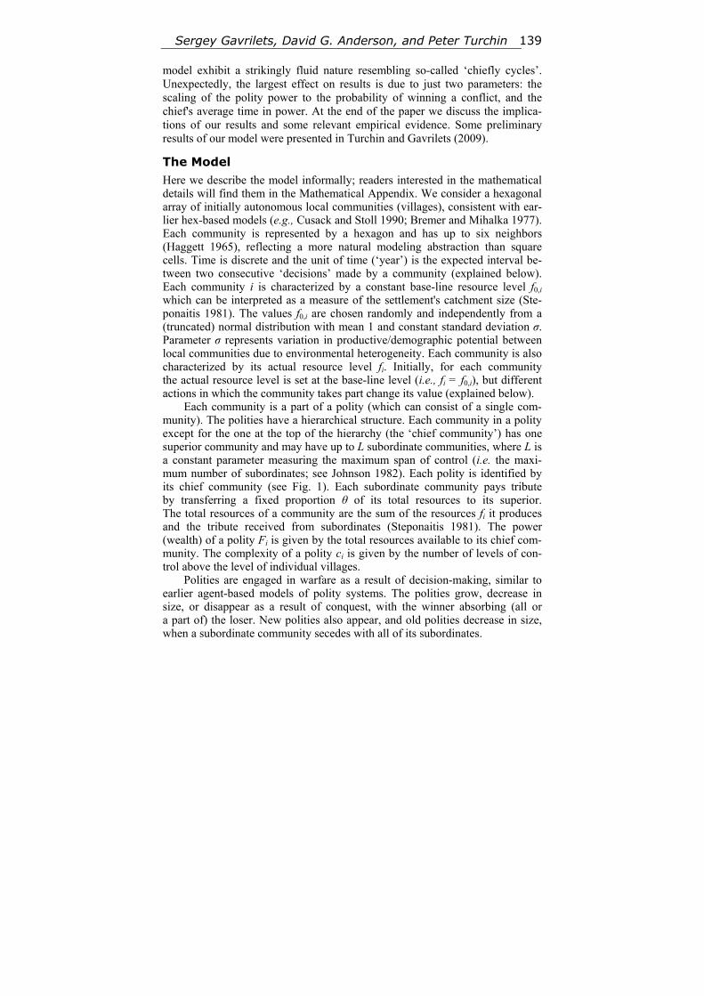
Sergey Gavrilets, David G. Anderson, and Peter Turchin 139
model exhibit a strikingly fluid nature resembling so-called ‘chiefly cycles’. Unexpectedly, the largest effect on results is due to just two parameters: the scaling of the polity power to the probability of winning a conflict, and the chief's average time in power. At the end of the paper we discuss the implica-tions of our results and some relevant empirical evidence. Some preliminary results of our model were presented in Turchin and Gavrilets (2009).
The Model Here we describe the model informally; readers interested in the mathematical details will find them in the Mathematical Appendix. We consider a hexagonal array of initially autonomous local communities (villages), consistent with ear-lier hex-based models (e.g., Cusack and Stoll 1990; Bremer and Mihalka 1977). Each community is represented by a hexagon and has up to six neighbors (Haggett 1965), reflecting a more natural modeling abstraction than square cells. Time is discrete and the unit of time (‘year’) is the expected interval be-tween two consecutive ‘decisions’ made by a community (explained below). Each community i is characterized by a constant base-line resource level f0,i which can be interpreted as a measure of the settlement's catchment size (Ste-ponaitis 1981). The values f0,i are chosen randomly and independently from a (truncated) normal distribution with mean 1 and constant standard deviation σ. Parameter σ represents variation in productive/demographic potential between local communities due to environmental heterogeneity. Each community is also characterized by its actual resource level fi. Initially, for each community the actual resource level is set at the base-line level (i.e., fi = f0,i), but different actions in which the community takes part change its value (explained below).
Each community is a part of a polity (which can consist of a single com-munity). The polities have a hierarchical structure. Each community in a polity except for the one at the top of the hierarchy (the ‘chief community’) has one superior community and may have up to L subordinate communities, where L is a constant parameter measuring the maximum span of control (i.e. the maxi-mum number of subordinates; see Johnson 1982). Each polity is identified by its chief community (see Fig. 1). Each subordinate community pays tribute by transferring a fixed proportion θ of its total resources to its superior. The total resources of a community are the sum of the resources fi it produces and the tribute received from subordinates (Steponaitis 1981). The power (wealth) of a polity Fi is given by the total resources available to its chief com-munity. The complexity of a polity ci is given by the number of levels of con-trol above the level of individual villages.
Polities are engaged in warfare as a result of decision-making, similar to earlier agent-based models of polity systems. The polities grow, decrease in size, or disappear as a result of conquest, with the winner absorbing (all or a part of) the loser. New polities also appear, and old polities decrease in size, when a subordinate community secedes with all of its subordinates.
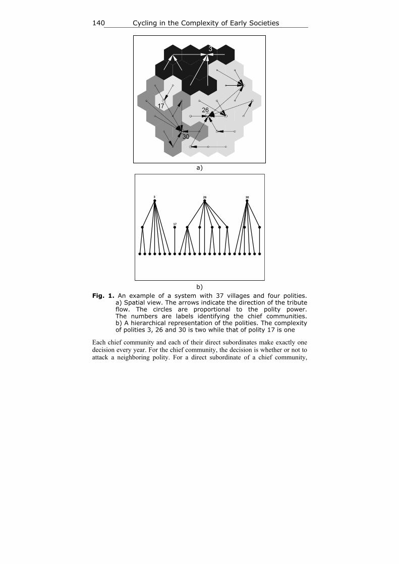
Cycling in the Complexity of Early Societies 140
a)
b)
Fig. 1. An example of a system with 37 villages and four polities. a) Spatial view. The arrows indicate the direction of the tribute flow. The circles are proportional to the polity power. The numbers are labels identifying the chief communities. b) A hierarchical representation of the polities. The complexity of polities 3, 26 and 30 is two while that of polity 17 is one
Each chief community and each of their direct subordinates make exactly one decision every year. For the chief community, the decision is whether or not to attack a neighboring polity. For a direct subordinate of a chief community,
3
17
26 30
3
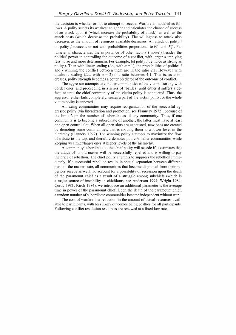
Sergey Gavrilets, David G. Anderson, and Peter Turchin 141
the decision is whether or not to attempt to secede. Warfare is modeled as fol-lows. A polity selects its weakest neighbor and calculates the chance of success of an attack upon it (which increase the probability of attack), as well as the attack costs (which decrease the probability). The willingness to attack also decreases as the amount of resources available decreases. An attack of polity i on polity j succeeds or not with probabilities proportional to iF and jF . Pa-
rameter α characterizes the importance of other factors (‘noise’) besides the polities' power in controlling the outcome of a conflict, with larger α implying less noise and more determinism. For example, let polity i be twice as strong as polity j. Then with linear scaling (i.e., with α = 1), the probabilities of polities i and j winning the conflict between them are in the ratio 2:1. However with quadratic scaling (i.e., with α = 2) this ratio becomes 4:1. That is, as α in-creases, polity strength becomes a better predictor of the outcome of conflict.
The aggressor attempts to conquer communities of the victim, starting with border ones, and proceeding in a series of ‘battles’ until either it suffers a de-feat, or until the chief community of the victim polity is conquered. Thus, the aggressor either fails completely, seizes a part of the victim polity, or the whole victim polity is annexed.
Annexing communities may require reorganization of the successful ag-gressor polity (via linearization and promotion, see Flannery 1972), because of the limit L on the number of subordinates of any community. Thus, if one community is to become a subordinate of another, the latter must have at least one open control slot. When all open slots are exhausted, new ones are created by demoting some communities, that is moving them to a lower level in the hierarchy (Flannery 1972). The winning polity attempts to maximize the flow of tribute to the top, and therefore demotes poorer/smaller communities while keeping wealthier/larger ones at higher levels of the hierarchy.
A community subordinate to the chief polity will secede if it estimates that the attack of its old master will be successfully repelled and is willing to pay the price of rebellion. The chief polity attempts to suppress the rebellion imme-diately. If a successful rebellion results in spatial separation between different parts of the master state, all communities that become disjointed from their su-periors secede as well. To account for a possibility of secession upon the death of the paramount chief as a result of a struggle among subchiefs (which is a major source of instability in chiefdoms, see Anderson 1994; Wright 1984; Cordy 1981; Kirch 1984), we introduce an additional parameter τ, the average time in power of the paramount chief. Upon the death of the paramount chief, a random number of subordinate communities become independent without war.
The cost of warfare is a reduction in the amount of actual resources avail-able to participants, with less likely outcomes being costlier for all participants. Following conflict resolution resources are renewed at a fixed low rate.
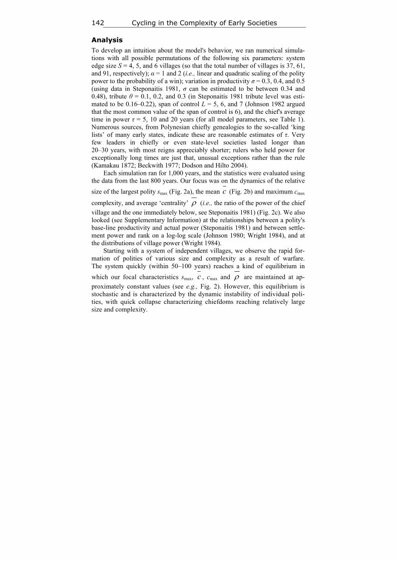
Cycling in the Complexity of Early Societies 142
Analysis
To develop an intuition about the model's behavior, we ran numerical simula-tions with all possible permutations of the following six parameters: system edge size S = 4, 5, and 6 villages (so that the total number of villages is 37, 61, and 91, respectively); α = 1 and 2 (i.e., linear and quadratic scaling of the polity power to the probability of a win); variation in productivity σ = 0.3, 0.4, and 0.5 (using data in Steponaitis 1981, σ can be estimated to be between 0.34 and 0.48), tribute θ = 0.1, 0.2, and 0.3 (in Steponaitis 1981 tribute level was esti-mated to be 0.16–0.22), span of control L = 5, 6, and 7 (Johnson 1982 argued that the most common value of the span of control is 6), and the chief's average time in power τ = 5, 10 and 20 years (for all model parameters, see Table 1). Numerous sources, from Polynesian chiefly genealogies to the so-called ‘king lists’ of many early states, indicate these are reasonable estimates of τ. Very few leaders in chiefly or even state-level societies lasted longer than 20–30 years, with most reigns appreciably shorter; rulers who held power for exceptionally long times are just that, unusual exceptions rather than the rule (Kamakau 1872; Beckwith 1977; Dodson and Hilto 2004).
Each simulation ran for 1,000 years, and the statistics were evaluated using the data from the last 800 years. Our focus was on the dynamics of the relative
size of the largest polity smax (Fig. 2a), the mean c (Fig. 2b) and maximum cmax
complexity, and average ‘centrality’ (i.e., the ratio of the power of the chief
village and the one immediately below, see Steponaitis 1981) (Fig. 2c). We also looked (see Supplementary Information) at the relationships between a polity's base-line productivity and actual power (Steponaitis 1981) and between settle-ment power and rank on a log-log scale (Johnson 1980; Wright 1984), and at the distributions of village power (Wright 1984).
Starting with a system of independent villages, we observe the rapid for-mation of polities of various size and complexity as a result of warfare. The system quickly (within 50–100 years) reaches a kind of equilibrium in
which our focal characteristics smax, c , cmax and are maintained at ap-
proximately constant values (see e.g., Fig. 2). However, this equilibrium is stochastic and is characterized by the dynamic instability of individual poli-ties, with quick collapse characterizing chiefdoms reaching relatively large size and complexity.
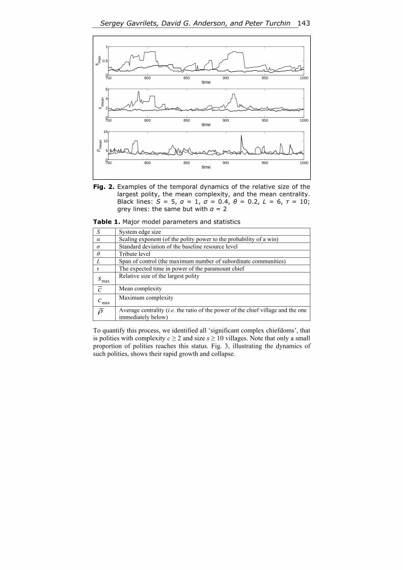
Sergey Gavrilets, David G. Anderson, and Peter Turchin 143
Fig. 2. Examples of the temporal dynamics of the relative size of the
largest polity, the mean complexity, and the mean centrality. Black lines: S = 5, α = 1, σ = 0.4, θ = 0.2, L = 6, τ = 10; grey lines: the same but with α = 2
Table 1. Major model parameters and statistics
S System edge size α Scaling exponent (of the polity power to the probability of a win) σ Standard deviation of the baseline resource level θ Tribute level L Span of control (the maximum number of subordinate communities) τ The expected time in power of the paramount chief
maxs Relative size of the largest polity
c Mean complexity
maxc Maximum complexity
Average centrality (i.e. the ratio of the power of the chief village and the one immediately below)
To quantify this process, we identified all ‘significant complex chiefdoms’, that is polities with complexity c ≥ 2 and size s ≥ 10 villages. Note that only a small proportion of polities reaches this status. Fig. 3, illustrating the dynamics of such polities, shows their rapid growth and collapse.
750 800 850 900 950 10000
0.5
1
time
s max
750 800 850 900 950 10000
2
4
6
time
c mea
n
750 800 850 900 950 10000
5
10
15
time
ρ mea
n

Cycling in the Complexity of Early Societies 144
a)
b)
Fig. 3. The dynamics of polities that have achieved a size of at least s = 10 and complexity c = 2. Different curves correspond to different chief villages: a) S = 5, α = 1, σ = 0.4, θ = 0.2, L = 6, τ = 10; b) the same but with α = 2
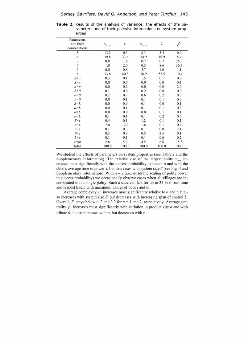
Sergey Gavrilets, David G. Anderson, and Peter Turchin 145
Table 2. Results of the analysis of variance: the effects of the pa-rameters and of their pairwise interactions on system prop-erties
Parameters and their
combinations maxs c maxc T
S 13.2 0.3 8.3 3.4 0.0 α 39.8 33.6 34.9 19.9 5.4 σ 0.8 1.6 0.7 0.7 25.0 θ 1.0 2.0 0.5 8.6 36.3 L 0.0 0.8 5.7 1.0 1.1 τ 33.8 40.8 38.9 55.5 10.4
S×α 0.3 0.1 1.5 0.1 0.0 S×σ 0.0 0.0 0.0 0.0 0.1 α×σ 0.0 0.2 0.0 0.0 2.0 S×θ 0.1 0.0 0.2 0.0 0.0 α×θ 0.2 0.7 0.6 0.2 0.0 σ×θ 0.0 0.1 0.1 0.1 0.3 S×L 0.0 0.0 0.1 0.0 0.1 α×L 0.0 0.1 0.1 0.1 0.3 σ×L 0.0 0.0 0.0 0.1 0.1 θ×L 0.1 0.1 0.1 0.2 0.5 S×τ 0.4 0.1 1.2 0.1 0.1 α×τ 7.0 12.9 1.8 0.1 0.4 σ×τ 0.1 0.3 0.1 0.0 2.1 θ×τ 0.3 0.9 0.5 2.5 0.1 L×τ 0.1 0.1 0.1 0.6 0.2 error 2.6 5.2 4.5 6.6 15.3 total 100.0 100.0 100.0 100.0 100.0
We studied the effects of parameters on system properties (see Table 2 and the Supplementary Information). The relative size of the largest polity smax in-creases most significantly with the success probability exponent α and with the chief's average time in power τ, but decreases with system size S (see Fig. 4 and Supplementary Information). With α = 2 (i.e., quadratic scaling of polity power to success probability) we occasionally observe cases when all villages are in-corporated into a single polity. Such a state can last for up to 35 % of run time and is most likely with maximum values of both τ and θ.
Average complexity c increases most significantly relative to α and τ. It al-so increases with system size S, but decreases with increasing span of control L. Overall, c stays below c. 2 and 3.3 for α = 1 and 2, respectively. Average cen-trality increases most significantly with variation in productivity σ and with
tribute θ; it also increases with α, but decreases with τ.
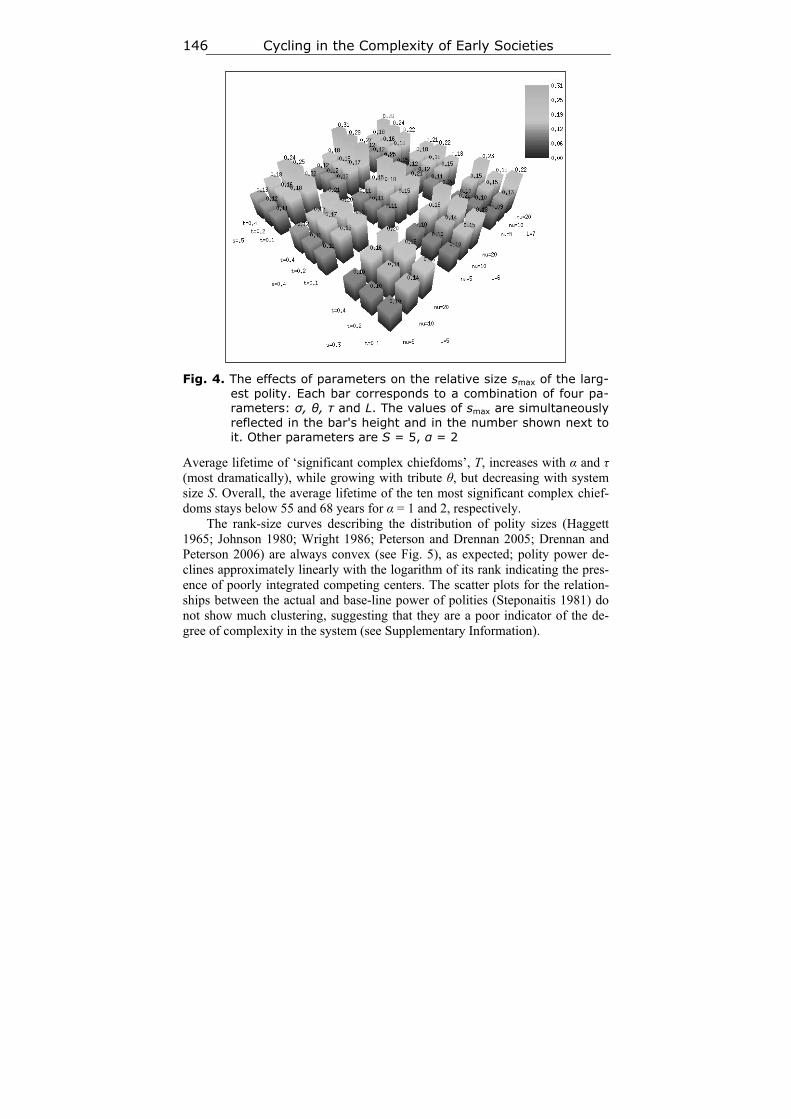
Cycling in the Complexity of Early Societies 146
Fig. 4. The effects of parameters on the relative size smax of the larg-est polity. Each bar corresponds to a combination of four pa-rameters: σ, θ, τ and L. The values of smax are simultaneously reflected in the bar's height and in the number shown next to it. Other parameters are S = 5, α = 2
Average lifetime of ‘significant complex chiefdoms’, T, increases with α and τ (most dramatically), while growing with tribute θ, but decreasing with system size S. Overall, the average lifetime of the ten most significant complex chief-doms stays below 55 and 68 years for α = 1 and 2, respectively.
The rank-size curves describing the distribution of polity sizes (Haggett 1965; Johnson 1980; Wright 1986; Peterson and Drennan 2005; Drennan and Peterson 2006) are always convex (see Fig. 5), as expected; polity power de-clines approximately linearly with the logarithm of its rank indicating the pres-ence of poorly integrated competing centers. The scatter plots for the relation-ships between the actual and base-line power of polities (Steponaitis 1981) do not show much clustering, suggesting that they are a poor indicator of the de-gree of complexity in the system (see Supplementary Information).
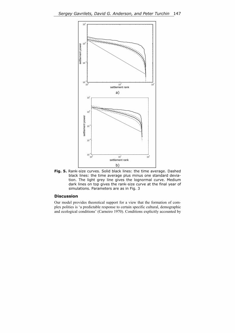
Sergey Gavrilets, David G. Anderson, and Peter Turchin 147
100
101
102
10−2
10−1
100
101
settlement rank
settl
emen
t pow
er
a)
100
101
102
10−3
10−2
10−1
100
101
settlement rank
settl
emen
t pow
er
b)
Fig. 5. Rank-size curves. Solid black lines: the time average. Dashed black lines: the time average plus minus one standard devia-tion. The light grey line gives the lognormal curve. Medium dark lines on top gives the rank-size curve at the final year of simulations. Parameters are as in Fig. 3
Discussion
Our model provides theoretical support for a view that the formation of com-plex polities is ‘a predictable response to certain specific cultural, demographic and ecological conditions’ (Carneiro 1970). Conditions explicitly accounted by
settl
emen
t pow
er
settl
em
ent
pow
er
settlement rank
settlement rank
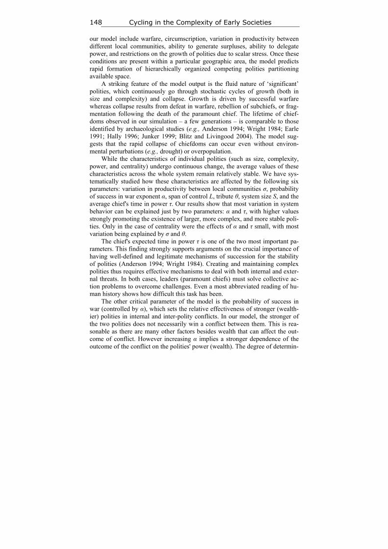
Cycling in the Complexity of Early Societies 148
our model include warfare, circumscription, variation in productivity between different local communities, ability to generate surpluses, ability to delegate power, and restrictions on the growth of polities due to scalar stress. Once these conditions are present within a particular geographic area, the model predicts rapid formation of hierarchically organized competing polities partitioning available space.
A striking feature of the model output is the fluid nature of ‘significant’ polities, which continuously go through stochastic cycles of growth (both in size and complexity) and collapse. Growth is driven by successful warfare whereas collapse results from defeat in warfare, rebellion of subchiefs, or frag-mentation following the death of the paramount chief. The lifetime of chief-doms observed in our simulation – a few generations – is comparable to those identified by archaeological studies (e.g., Anderson 1994; Wright 1984; Earle 1991; Hally 1996; Junker 1999; Blitz and Livingood 2004). The model sug-gests that the rapid collapse of chiefdoms can occur even without environ-mental perturbations (e.g., drought) or overpopulation.
While the characteristics of individual polities (such as size, complexity, power, and centrality) undergo continuous change, the average values of these characteristics across the whole system remain relatively stable. We have sys-tematically studied how these characteristics are affected by the following six parameters: variation in productivity between local communities σ, probability of success in war exponent α, span of control L, tribute θ, system size S, and the average chief's time in power τ. Our results show that most variation in system behavior can be explained just by two parameters: α and τ, with higher values strongly promoting the existence of larger, more complex, and more stable poli-ties. Only in the case of centrality were the effects of α and τ small, with most variation being explained by σ and θ.
The chief's expected time in power τ is one of the two most important pa-rameters. This finding strongly supports arguments on the crucial importance of having well-defined and legitimate mechanisms of succession for the stability of polities (Anderson 1994; Wright 1984). Creating and maintaining complex polities thus requires effective mechanisms to deal with both internal and exter-nal threats. In both cases, leaders (paramount chiefs) must solve collective ac-tion problems to overcome challenges. Even a most abbreviated reading of hu-man history shows how difficult this task has been.
The other critical parameter of the model is the probability of success in war (controlled by α), which sets the relative effectiveness of stronger (wealth-ier) polities in internal and inter-polity conflicts. In our model, the stronger of the two polities does not necessarily win a conflict between them. This is rea-sonable as there are many other factors besides wealth that can affect the out-come of conflict. However increasing α implies a stronger dependence of the outcome of the conflict on the polities' power (wealth). The degree of determin-
Sergey Gavrilets, David G. Anderson, and Peter Turchin 149
ism in the conflict resolution (and thus, parameter α) is expected to increase with economic and political development (Carneiro 1970, 1981; Collins 1986). Note that in our simulations, polities conquering the whole simulation domain are observed only with α = 2.
Our model shows no qualitative differences between polities with a single level of control above the level of individual villages (‘simple chiefdoms’) and polities with two or more levels of control (‘complex chiefdoms’ or ‘states’). During each individual run, the number of control levels is not stable but changes dynamically and therefore cannot by itself serve as an indicator of the presence of ‘true’ states. Our results support Carneiro's (1981: 38) insight that ‘the transcending of local sovereignty and the aggregation of previously auton-omous villages into chiefdoms was a critical step in political development – probably the most important one ever taken. It crossed a threshold, and once crossed, unlimited further advance in the same direction became possible. The emergence of chiefdoms was a qualitative step. Everything that followed, including the rise of states and empires, was, in a sense merely quantitative’.
In our simulations it was possible for polities to conquer the whole spatial domain, or a significant part of it. However, our analyses also show that such polities are relatively short-lived. A major reason for this is the relative ease of rebellion within larger polities. Additionally, our model explicitly assumes that any ‘internal specialization’ is absent and that all mechanisms for autonomous existence of a rebellious province are already in place. This model behavior thus further emphasizes, through the effect of its absence, the importance of ‘internal specialization’ for the emergence of large and stable polities (Flannery 1972; Wright 1977, 1984).
Implications for Archaeological Research
Due to temporal resolution limitations archaeological analyses of settlement hierarchies typically combine sites occupied over intervals of a half century to, sometimes, hundreds of years. The hierarchies reconstructed by archaeologists are commonly displayed as a series of maps showing site sizes during different periods, often separated by a century or more, or else histograms or rank size plots (Wright and Johnson 1975; Wright 1977, 1984, 1986; Johnson 1980; Hal-ly 1996; McAndrews et al. 1997; Spencer and Redmond 2001; Liu and Chen 2003; Peterson and Drennan 2005; Drennan and Peterson 2006). These recon-structions suggest rigid formal hierarchies and static political landscapes. Our analyses, in contrast, indicate that at a finer temporal scale the various factors that produce these archaeological signatures are much more dynamic. This re-sult is in agreement with written records of historical events (when available; e.g., Earle 1987, 1991).
Our estimates of chiefdom duration are comparable with those based on ar-chaeological evidence. In studying Southeastern Mississippian chiefdoms, Hal-
Cycling in the Complexity of Early Societies 150
ly (1993) examined the time periods when occupation and mound construc-tion occurred at 47 mound centers in central and northern Georgia. He con-cluded that ‘paramount chiefdoms must have been unstable and short lived’ while ‘simple and complex chiefdoms endured for as much as a century or more’ (Hally 1993). The actual duration of phases, or periods of occupation and construction in his analysis (Ibid.: 145), however, could not be resolved much below 75–100 years. Hally extended this analysis in a second paper (Hally 1996) examining 45 mound centers, and including episodes of mound stage construction. Where evidence for numbers of internal mound construc-tion stages was available, duration of occupation was estimated to be between 75 and 100 years, with the average number of years per stage ranging from 12 to 25 years at the best understood sites (Hally 1996). This span may represent the duration of a chiefly leader, or generation. At 29 of the 45 mound centers, only a single period of use is currently known, indicating most ‘chiefdoms’ locally lasted no more than 75–100 years, and perhaps appreciably less (Hally 1996).
In a follow up, Hally (2006: 27) argued that ‘as many as 47 distinct chief-doms rose and fell’ in 27 locations during the Mississippian period in northern Georgia (some locations were occupied repeatedly, often with gaps in occupa-tion of a century or more). The numbers of chiefdoms in his sample fluctuated between 8 and 17 during the period of 1000–1500 CE (Hally 2006). Many poli-ties in the sample were single-mound simple chiefdoms (Hally 2006).
Blitz and Livingood (2004) used mound volume as an alternate means of measuring regional settlement hierarchies, using a sample of sites from across the southeast USA. For a sample of 35 mounds they recorded a mound volume index (basal length × basal width × height / 1000), the number of major mound-construction stages, the duration of mound use in years, and the number of mounds at the site where the sample mound was found (Ibid.: 293). Their anal-ysis, while geographically broader than Hally's, yielded generally similar re-sults, noting average mound center ‘duration of use range is 100–450 years, with a mean of 183 years and a median of 150 years. Also, there appears to be a rough periodicity in mound construction: the average occupation span per construction layer is 25–50 years’ (Ibid.: 296). They were able to demonstrate that mound stage construction might fall into two cycles, one of c. 12–18 years, and another of c. 25–50 year spacing (Ibid.: 297).
Our finding that the duration of a chief's reign is a significant parameter parallels that in the literature on state fiscal organization. In this literature, the discount rate of rulers (that is, their expected time in office) is shown to be a major determinant of the kind of taxation system employed, which in turn has various implications for society, for example, for political stability of the Ro-man state and Ptolemaic Egypt (Kiser and Kane 2007; Levi 1988; Monson 2007).
Sergey Gavrilets, David G. Anderson, and Peter Turchin 151
In our model individual villages differ only in their base-line productivity and geographic location but otherwise have equal ability to form complex so-cieties. In human history some polities had a headstart, allowing them to achieve large size initially (e.g., San Miguel Mogote or El Mirador in Meso-america; Uruk and Susa in Mesopotamia; Aspero in South America; see Ser-vice 1975); but the strategies for complex polities buildup and maintenance would have spread quickly in a Darwinian fashion as a result of conquest and imitation. Therefore once chiefdoms appeared, their organizational form would itself have tended to spread, as neighboring societies adopted it for reasons ranging from emulation to self defense (Carneiro 1981; Anderson 1994).
Conclusion
The dynamics generated by our model, in which hierarchical societies tend to achieve at most medium levels of complexity, and only for relatively short pe-riods of time, resembles the chiefly cycles observed prior to sustained Western contact in eastern North America, southern Central America and northern South America, Oceania, southeast Asia and the Philippines, and across large parts of sub-Saharan Africa (e.g., Wright 1984; Marcus 1992; Earle 1991; Anderson 1994; Cordy 1981; Junker 1999; Drennan and Peterson 2006).
The model developed here can be extended in a number of ways. For ex-ample, instead of a simple conquest mechanism, one can consider a more nu-anced dynamic in which external threat of conquest (or raiding) induces a greater degree of cooperation between lower-level groups, which results in a more stable higher-level polity. According to Cioffi-Revilla's canonical the-ory (2005), such a (‘fast’) process is common for producing stronger institu-tions of government. One possible direction is to generalize the model to allow for the formation of coalitions between different polities (Carneiro 1998; see Gavrilets et al. 2008 for a possible dynamic approach). Also, to adapt the model for describing larger spatial scales (e.g., as necessary for modeling the origin of states and empires), changes in population densities need to be considered, as well as the propensity for cooperation (and, conversely, conflict) should be allowed to depend on cultural similarity/dissimilarity between the agents.
Over the past several decades mathematical methods and techniques have become very important in life sciences and social sciences (Spencer 1998; Ciof-fi-Revilla 2002; Bentley and Maschner 2008; Costopoulos 2008; Kohler et al. 2005). In particular, mathematical and computational modeling are powerful tools for better understanding the origins of new species (Gavrilets 2004) and of general rules of biological diversification (Gavrilets and Losos 2009). Agent-based simulation modeling efforts like those advanced here offer fruitful ave-nues for future research on general patterns in historical dynamics and on the emergence and diversification of human societies (Turchin 2003, 2006, 2009).
Cycling in the Complexity of Early Societies 152
References
Adams R. M. 1966. The Evolution of Urban Society. Chicago, IL: Aldine Press.
Anderson D. G. 1994. The Savannah River Chiefdoms: Political Change in the Late Prehistoric Southeast. Tuscaloosa, AL: University of Alabama Press.
Anderson D. G. 1996. Fluctuations between Simple and Complex Chiefdoms: Cycling in the Late Prehistoric Southeast. Political Structure and Change in the Prehistoric Southeastern United States / Ed. by J. F. Scarry, pp. 231–252. Gainesville, FL: University Press of Florida.
Beckwith M. W. 1977. Hawaiian Mythology. Honolulu, HI: University of Hawaii Press.
Bentley R. A., and Maschner H. D. G. 2008. Complexity Theory. Handbook of Archaeological Theories / Ed. by R. A. Bentley, H. D. G. Maschner, and C. Chippindale, pp. 245–270. Lanham, MD: AltaMira Press.
Blitz J., and Livingood P. 2004. Sociopolitical Implications of Mississippian Mound Volume. American Antiquity 69(2): 291–301.
Bremer S. A., and Mihalka M. 1977. Machiavelli in Machina: Or Politics Among Hexagons. Problems of the World Modeling: Political and Social Implications / Ed. by K. W. Deutsch, B. Fritsch, H. Jaquaribe, and A. S. Markovits, pp. 303–337. Cambridge: Ballinger Publishing.
Carneiro R. L. 1970. A Theory of the Origin of State. Science 169: 733–738.
Carneiro R. L. 1981. The Chiefdom: Precursor of State. The Transition to Statehood in the New World / Ed. by G. D. Jones, and R. R. Kautz, pp. 37–79. Cambridge: Cambridge University Press.
Carneiro R. 1998. What Happened at the Flashpoint? Conjectures on Chiefdom Formation at the Very Moment of Conception. Chiefdoms and Chieftaincy in the Americas / Ed. by E. M. Redmond, pp. 18–42. Gainesville, FL: University Press of Florida.
Cederman L.-E. 1997. Emergent Actors in World Politics. Princeton, NJ: Princeton University Press.
Cederman L.-E., and Girardin L. 2010. Growing Sovereignty: Modeling the Shift from Indirect to Direct Rule. International Studies Quarterly 48: 27–48.
Childe V. G. 1950. The Urban Revolution. The Town Planning Review 21: 3–17.
Cioffi-Revilla C. 2000. Ancient Warfare: Origins and Systems. Handbook of War Studies II / Ed. by M. I. Midlarsky, pp. 59–89. Ann Arbor, MI: University of Michigan Press.
Cioffi-Revilla C. 2002. Invariance and Universality in Social Agent-based Simulations. Proceedings of the National Academy of Sciences 99: 7314–7316.
Cioffi-Revilla C. 2005. A Canonical Theory of Origins and Development of Social Complexity. Journal of Mathematical Sociology 29: 133–153.
Cioffi-Revilla C., and Landman T. 1999. Evolution of Maya Polities in the Ancient Mesoamerican System. International Studies Quarterly 43: 559–598.
Collins R. 1986. Weberian Sociological Theory. New York: Cambridge University Press.
Sergey Gavrilets, David G. Anderson, and Peter Turchin 153
Cordy R. H. 1981. A Study of Prehistoric Social Change. The Developmnent of Complex Societies in the Hawaiian Islands. New York: Academic Press.
Costopoulos A. 2008. Simulating Society. Handbook of Archaeological Theories / Ed. by R. A. Bentley, H. D. G. Maschner, and C. Chippindale, pp. 273–281. Lanhan, MD: AltaMira Press.
Cusack T. R., and Stoll R. J. 1990. Exploring Realpolitik. Probing International Rela-tions Theory with Computer Simulation. Boulder, CO: Lynne Rienner Publishers.
Dacey M. F. 1969. A Probability Model for the Rise and Decline of States. Peace Re-search Society Papers 14: 147–153.
Dacey M. F. 1974. A Model of Political Integration and Its Use in the Reconstruction of a Historical Situation. Locational Approaches to Power and Conflict / Ed. by K. R. Cox, D. R. Reynolds, and S. Rokkan, pp. 213–230. New York: SAGE Publica-tions.
Dodson A., and Hilto D. 2004. The Complete Royal Families of Ancient Egypt: A Genealogical Sourcebook of the Pharaohs. New York: Thames and Hudson.
Drennan R. D., and Peterson C. E. 2006. Patterned Variation in Prehistoric Chief-doms. Proceedings of the National Academy of Sciences 103: 3960–3967.
Earle T. K. 1987. Chiefdoms in Archeological and Ethnohistorical Perspective. Annual Review of Anthropology 16: 279–308.
Earle T. K. 1991. Chiefdoms: Power, Economy and Ideology. New York: Cambridge University Press.
Earle T. K. 1997. How Chiefs Come to Power. Stanford, CA: Stanford University Press.
Engels F. 1884. Origins of the Family, Private Property, and the State. Selected Readings in Two Volumes. Vol. 2 / Ed. by K. Marx, and F. Engels, pp. 185–326. Moscow: Foreign Languages Press.
Ferguson R. B. 1984. Warfare, Culture, and Environment. Orlando, FL: Academic Press.
Ferguson Y. H., and Mansbach R. W. 1996. Polities: Authority, Identities, and Change. Columbia, SC: University of South Carolina Press.
Flannery K. V. 1972. The Cultural Evolution of Civilizations. Annual Review of Ecology and Systematics 3: 399–426.
Fried M. H. 1967. The Evolution of Political Society. New York: Random House.
Gavrilets S. 2004. Fitness Landscapes and the Origin of Species. Princeton, NJ: Princeton University Press.
Gavrilets S., Duenez-Guzman E. A., and Vose M. D. 2008. Dynamics of Alliance Formation and the Egalitarian Revolution. PLOS ONE 3(10): e3293.
Gavrilets S., and Losos J. 2009. Adaptive Radiation: Contrasting Theory with Data. Science 323: 732–737.
Haas J. 2004. The Anthropology of War. Cambridge: Cambridge University Press.
Haggett P. 1965. Locational Analysis in Human Geography. London: Edward Arnold.
Hall T. D. 2001. Chiefdoms, States, Cycling, and World-Systems Evolution: A Review Essay. Journal of World-Systems Research 7: 91–99.
Cycling in the Complexity of Early Societies 154
Hally D. J. 1993. The Territorial Size of Mississippian Chiefdoms. Archaeology of Eastern North America Papers in Honor of Stephen Williams. Archaeological Report No. 25 / Ed. by J. B. Stoltman, pp. 143–168. Jackson, MS: Mississippi Department of Archives and History.
Hally D. J. 1996. Platform Mound Construction and the Instability of Mississippian Chiefdoms. Political Structure and Change in the Prehistoric Southeastern United States / Ed. by J. F. Scarry, pp. 92–127. Gainesville, FL: University Press of Florida.
Hally D. J. 2006. The Nature of Mississippian Regional Systems. Light on the Path: The Anthropology and History of the Southeastern Indians / Ed. by T. J. Pluckhahn and R. Ethridge, pp. 26–42. Tuscaloosa, AL: University of Alabama Press.
Johnson G. A. 1980. Rank Size Convexity and System Integration. Economic Geography 56(3): 234–247.
Johnson G. A. 1982. Organizational Structure and Scalar Stress. Theory and Expla-nation in Archaeology / Ed. by C. Renfrew, M. Rowlands, and B. A. Segraves, pp. 389–421. New York: Academic Press.
Junker L. L. 1999. Raiding, Trading, and Feasting: The Political Economy of Philippine Chiefdoms. Honolulu: University of Hawaii Press.
Kamakau S. M. 1872. Ruling Chiefs of Hawaii. Honolulu: Kamehameha Schools Press.
Keely L. H. 1997. War before Civilization: The Myth of the Peaceful Savage. New York, NY: Oxford University Press.
Kirch P. V. 1984. The Evolution of the Polynesian Chiefdoms. Cambridge: Cambridge University Press.
Kiser E., and Kane D. 2007. The Perils of Privatization: How the Characteristics of Principals Affected Tax Farming in the Roman Republic and Empire. Social Science History 31(2): 191–212.
Kohler T., Gumerman G., and Reynolds R. 2005. Simulating Ancient Societies. Scientific American 293(1): 76–82.
Kurella D. 1998. The Muisca. Chiefdoms in Transition. Chiefdoms and Cieftaincy in the Americas / Ed. by E. M. Redmond, pp. 189–216. Gainsville, FL: University Press of Florida.
Lenin V. 1918. The State and Revolution. Collected Works. Vol. 25, pp. 381–492. Moscow: Progress Publishers.
Levi M. 1988. Of Rule and Revenue. Berkeley, CA: University of California Press.
Liu L., and Chen X. 2003. State Formation in Early China. London: Duckworth.
Marcus J. 1992. Political Fluctuations in Mesoamerica. National Geographic Research and Exploration 8(4): 392–411.
Marcus J. 1998. The Peaks and Valleys of Ancient States an Extension of the Dynamic Model. Archaic States / Ed. by G. Feinman and J. Marcus, pp. 59–94. Santa Fe, NM: SAR Press.
McAndrews T. L., Albarracin-Jordan J., and Bermann M. 1997. Regional Settlement Patterns in the Tiwanaku Valley of Bolivia. Journal of Field Archaeology 24: 67–83.
Sergey Gavrilets, David G. Anderson, and Peter Turchin 155
Monson A. 2007. Rule and Revenue in Egypt and Rome: Political Stability and Fiscal Institutions. Historical Social Research 32(4): 252–274.
Peterson C. E., and Drennan R. D. 2005. Communities, Settlements, Sites, and Sur-veys: Regional-scale Analysis of Prehistoric Human Interaction. American Antiquity 70(1): 5–30.
Service E. R. 1975. Origins of the State and Civilization. The Process of Cultural Evo-lution. New York: Norton and Company.
Service E. R. 1978. Classical Theories of the Origin of Government. Origins of the State / Ed. by R. Cohen, and E. R. Service, pp. 21–34. Philadelphia, PA: Institute for the Study of Human Issues.
Spencer C. S. 1998. A Mathematical Model of Primary State Formation. Cultural Dynamics 10(1): 5–20.
Spencer C. S. 2010. Territorial Expansion and Primary State Formation. Proceedings of the National Academy of Sciences of the United States of America 107(16): 7119–7126.
Spencer C. S., and Redmond E. M. 2001. Multilevel Selection and Political Evolution in the Valley of Oaxaca, 500–100 B.C. Journal of Anthropological Archaeology 20: 195–229.
Steponaitis V. P. 1978. Location Theory and Complex Chiefdoms: A Mississippian Example. Mississippian Settlement Patterns / Ed. by B. D. Smith, pp. 417–453. New York: Academic Press.
Steponaitis V. P. 1981. Settlement Hierarchies and Political Complexity in Nonmarket Societies: The Formative Period of the Valley of Mexico. American Anthropologist 83: 320–363.
Trigger B. G. 2003. Understanding Early Civilizations: A Comparative Study. Cambridge: Cambridge University Press.
Turchin P. 2003. Historical Dynamics: Why States Rise and Fall. Princeton, NJ: Princeton University Press.
Turchin P. 2006. War and Peace and War: The Life Cycles of Imperial Nations. New York: Pi Press.
Turchin P. 2009. A Theory for Formation of Large Empires. Journal of Global History 4: 191–207.
Turchin P., and Gavrilets S. 2009. Evolution of Complex Hierarchical Societies. So-cial Evolution and History 8(2): 167–198.
Webster D. 1975. Warfare and the Evolution of the State: A Reconsideration. American Antiquity 40: 464–470.
Wittfogel K. A. 1957. Oriental Despotism: A Comparative Study of Total Power. New Haven, CT: Yale University Press.
Wright H. T. 1977. Recent Research on the Origin of the State. Annual Reviews of Anthropology 6: 379–397.
Wright H. T. 1984. Prestate Political Formations. On the Evolution of Complex Societies. Essays in Honor of Harry Hoijer / Ed. by W. Sander, H. T. Wright, and R. M. Amams, pp. 41–77. Malibu, CA: Undena Press.
Cycling in the Complexity of Early Societies 156
Wright H. T. 1986. The Evolution of Civilizations. American Archeology Past and Future / Ed. by D. J. Meltzer, pp. 323–365. Washington: Smithsonian Institution Press.
Wright H. T., and Johnson G. A. 1975. Population, Exchange, and Early State Formation in Southwestern Iran. American Anthropology 77: 267–289.
Mathematical Appendix
Here we provide some additional details on the model and simulations. The model was implemented in the Matlab.
Attacks. A polity may attack only its weakest neighbor. The attack of pol-ity i on polity j is successful with probability
iij
i j
FP
F F
, (Eq. 1)
where Fi is the power of polity i, and α is the success probability exponent. Pol-ity i will attack polity j only if it estimates that the attack will be successful, is willing to pay the cost of warfare, and is not too devastated by previous war-fare. Specifically, the probability of attack is set to
,0
exp[ ] iij ij ij
i
FA P c
F . (Eq. 2)
Here the first term is the probability of winning (estimated by the potential aggressor via ‘scenario building’). The second term accounts for a negative effect of costs of warfare, cij (defined below), on the willingness to attack; β > 0 is a parameter. The third term accounts for a reduction in the willingness to attack caused by recent conflicts (and ensuing drop in available resources); Fi,0 is the maximum possible power of the i-th polity (observed at maximum possi-ble level of resources; i.e., if all fi = fi,0). If attack is not successful, a war ends in a draw.
We assume that attacks proceed through one or more stages. At the first stage, the target is the wealthiest border community of the weakest neighbor. The victim repels the attack successfully with probability Qij = 1 – Pij. If the attack was successful, the aggressor proceeds to attack the superior of the tar-get. Now the probability that the victim repels the attack successfully is reduced to (1 – γ)Qij, where 0 ≤ γ <1 is a parameter characterizing the ‘loser effect’ (e.g., due to demoralization). If the second attack is successful, the aggressor pro-ceeds to attack the superior of the superior of the target and so on. The process stops when an attack is repelled or when the chief community of the victim po-lity is conquered. In the former case, the aggressor seizes a part of the victim polity that was subordinate to the community attacked at the last successful attack. In the latter case, the whole victim's polity is seized.
Linearization and promotion. Polity i attempts to maximize the flow of tribute by the processes of linearization and promotion, after Flannery (1972),
Sergey Gavrilets, David G. Anderson, and Peter Turchin 157
subject to geographic restrictions and restrictions on the number of subordi-nates. If the chief community i has an open control slot, it will control polity j directly. If there are no open control slots, then the chief community will con-trol directly the L wealthiest communities chosen (i.e., promoted) from the set of its L subordinates and the newly conquered polity j. The remaining (i.e., the poorest) community will be demoted and reattached to its geographi-cally closest neighbor of the higher rank (i.e., by-passed in a process akin to linearization). If this neighbor has already filled all its control slots, further re-arrangements will follow according to the same strategy.
Costs. Different actions (i.e., attack, defense, rebellion, or suppression of rebellion) reduce the actual resource level for all participants by a factor (1 − c) where the cost c of an action is equal to a constant δ times the probability of loss for the winner (0 < δ ≤ 1). That is, if Pij is the probability that an attack of polity i on polity j is successful, then the cost of a successful attack is
(1 )ijc P , (Eq. 3a)
whereas the cost of an unsuccessful attack is
ijc P . (Eq. 3b)
This simple model captures the idea that more likely outcomes are less costly to all participants. For attacks involving several stages, costs are com-bined multiplicatively.
Resource dynamics. Each year the actual resource level fi grows towards its baseline level fi,0 at an exponential rate. Specifically, we define the half-life of resource recovery r measured in years so that it takes r peaceful years for the resource to grow from 1 − δ to 1 − δ/2.
Implementation rules. We use a ‘parallel’ implementation of the model in which different actions happen simultaneously rather then sequentially. To handle multiple events potentially involving the same polity we use the fol-lowing rules: 1) A polity that is subject to a rebellion does not attack other poli-ties. 2) A polity that is subject to a rebellion is not attacked by other polities. (The justification: since dealing with the rebellion will make the polity weaker, potential attackers would prefer to wait and attack later.) 3) If there are multiple rebellions within a polity, the polity's power is divided proportionally and mul-tiple suppression attempts occur simultaneously.
Supplementary Information
1. Sample movies with α = 1 and α = 2. Other parameters are at the mid-points of the ranges used (S = 6, σ = 0.3, θ = 0.2, L = 6, τ = 10).
The movies are currently available at http://neko.bio.utk.edu/~sergey/ chiefdoms/chiefdoms.html.
2. Detailed simulation results for S = 4, S = 5, S = 6.

Cycling in the Complexity of Early Societies 158
The files are currently available at http://neko.bio.utk.edu/~sergey/chief doms/chiefdoms.html.
3. Effects of parameters on the properties of the system. The files are currently available at http://neko.bio.utk.edu/~sergey/chief
doms/chiefdoms.html.
Acknowledgement
We thank the reviewers for valuable comments and suggestions. This research was supported by a Guggenheim Fellowship (SG) and by the National Science Foundation Grant NSF-HSD SES-0527720 (PT).
History & Mathematics: Trends and Cycles 2014 159–189
159
5
Demographic-Structural Theory and the Roman Dominate
David C. Baker
Abstract
This article uses the theory of secular cycles to examine the Eastern and West-ern Roman Empires in roughly 285–700 CE. The analysis suggests that the Eastern Empire conforms to an almost ‘standard’ cycle during that time. The Western Roman Empire, on the other hand, appears to expand until 350 CE and then decline again, long before the Germanic invasions of the fifth century. This decline may have been due to elite dynamics and the extremely top-heavy social pyramid in the fourth century West. Elite overproduction and infighting may have cut short the West's expansion phase and led to a prema-ture decline. If correct, it is possible that demographic-structural theory ex-plains the decline and fall of the Roman Empire.
Keywords: Cliodynamics, Roman Empire, Dominate, population, history.
Introduction
The work of Peter Turchin over the last decade has shown that population pres-sure exerts a powerful influence over socio-political instability, historical events, and the ebb and flow of state power (Turchin 2003, 2006; Turchin and Nefedov 2009). The dynamics can be identified in cycles of a few hundred years of expansion and contraction.1 One interesting test of theory has recently been done on Pueblo societies by Kohler et al. (2009: 290–291). Here is a rough overview of the theory. When a population is low, there is plenty of food and a labour shortage, and so food prices are low and wages are high. A population enjoys a decent standard of living. This dynamics translates into political stability. As a result, the population tends to grow. This is the expan-sion phase. Eventually a population approaches its carrying capacity resulting in shortages of food and an oversupply of labour. Prices rise, wages drop, and the standard of living declines. The average person is paid less and has to pay more for the basic essentials. Famines increase in severity, the susceptibility of
1 The average appears to be roughly 300 years for a full cycle, but depends greatly on specific con-
ditions.
The Roman Dominate 160
people to disease also increases, as does the possibility of widespread epidem-ics. At the same time, it is a ‘golden age’ for the elite. Landowners pay lower wages and charge higher rents. Middling landowners are forced off their farms and land is concentrated in the hands of the few. The inequality gap widens. Elite numbers and appetites grow. This is the ‘stagflation’ phase (Turchin and Nefedov 2009: 10–13).
Then a society hits a crisis. People starve, social cohesion collapses, the number of people living at subsistence level grows, grain reserves disappear, diseases ravage a malnourished population, there are rural and urban uprisings and, ultimately, the population declines. As the general population shrinks, the elites, cushioned by their status and their wealth, do not die at the same rate. The social pyramid becomes top-heavy. Elites begin to see their incomes shrink. The result is elite infighting and competition for the resources of the state. In this period faction and civil war are prevalent. Thus the first crisis, spurred mainly by demographic causes, is followed by a second crisis or ‘de-pression’ which is largely man-made. The man-made crisis holds recovery down, and this can last for decades. Eventually, however, a population does rebound. Elite numbers are reduced. Low numbers in the general population combined with high wages and low food prices lead to another period of expan-sion, peace, and stability.
In this paper I apply the demographic-structural theory to the period of the Roman Dominate. First I review the two secular cycles that were experienced by the Roman Republic and Empire before 285 CE. Next I consider the demo-graphic-structural trends in the Eastern Empire between 285 and 628 CE. Then I look at the divergent cycle in the West between 285 and 400 CE and possible demographic-structural explanations for the downfall of the Western Roman Empire.
The Republican Cycle (350–30 BCE) and Principate Cycle (30 BCE – 285 CE) Rome underwent two previous cycles that have been examined by Peter Tur-chin and Sergey Nefedov in Secular Cycles (2009). There is even a theoretical case to be made for an even earlier cycle spanning 650 to 350 BCE, seeing ex-pansion and stagflation for the first 150 years, and crisis and depression falling around the overthrow of Tarquin the Proud and the establishment of the Repub-lic. The Republican Cycle entered an expansion phase during which Rome es-tablished hegemony over the Italian peninsula from c. 350 onward. The popula-tion losses of the Second Punic War (218–201), an exogenous variable, might explain the elongated duration of the Republican cycle. Stagflation set in around 180, and a disintegrative trend began somewhere between 133 and 90, more likely the latter, and lasted through the wars of Sulla, Caesar, and the Tri-umvirate until around 30 BCE (Turchin and Nefedov 2009: 176–210). The following period, the Principate cycle (30 BCE – 285 CE), precedes
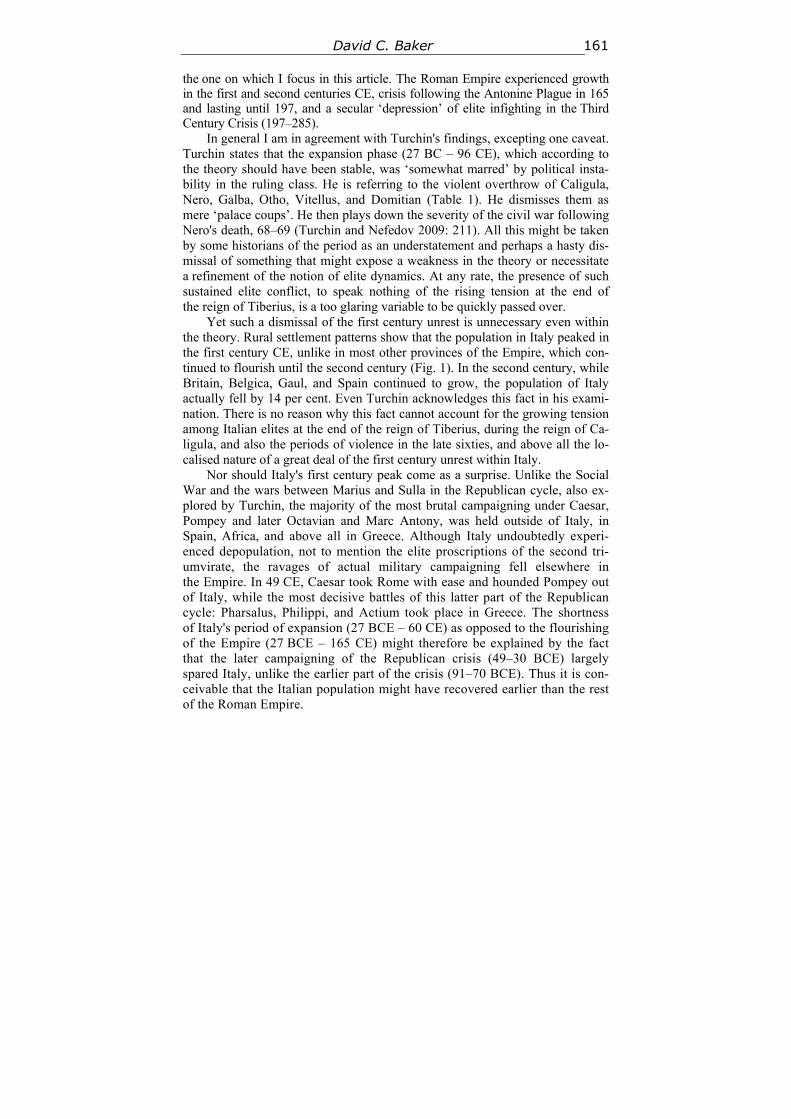
David C. Baker 161
the one on which I focus in this article. The Roman Empire experienced growth in the first and second centuries CE, crisis following the Antonine Plague in 165 and lasting until 197, and a secular ‘depression’ of elite infighting in the Third Century Crisis (197–285).
In general I am in agreement with Turchin's findings, excepting one caveat. Turchin states that the expansion phase (27 BC – 96 CE), which according to the theory should have been stable, was ‘somewhat marred’ by political insta-bility in the ruling class. He is referring to the violent overthrow of Caligula, Nero, Galba, Otho, Vitellus, and Domitian (Table 1). He dismisses them as mere ‘palace coups’. He then plays down the severity of the civil war following Nero's death, 68–69 (Turchin and Nefedov 2009: 211). All this might be taken by some historians of the period as an understatement and perhaps a hasty dis-missal of something that might expose a weakness in the theory or necessitate a refinement of the notion of elite dynamics. At any rate, the presence of such sustained elite conflict, to speak nothing of the rising tension at the end of the reign of Tiberius, is a too glaring variable to be quickly passed over.
Yet such a dismissal of the first century unrest is unnecessary even within the theory. Rural settlement patterns show that the population in Italy peaked in the first century CE, unlike in most other provinces of the Empire, which con-tinued to flourish until the second century (Fig. 1). In the second century, while Britain, Belgica, Gaul, and Spain continued to grow, the population of Italy actually fell by 14 per cent. Even Turchin acknowledges this fact in his exami-nation. There is no reason why this fact cannot account for the growing tension among Italian elites at the end of the reign of Tiberius, during the reign of Ca-ligula, and also the periods of violence in the late sixties, and above all the lo-calised nature of a great deal of the first century unrest within Italy.
Nor should Italy's first century peak come as a surprise. Unlike the Social War and the wars between Marius and Sulla in the Republican cycle, also ex-plored by Turchin, the majority of the most brutal campaigning under Caesar, Pompey and later Octavian and Marc Antony, was held outside of Italy, in Spain, Africa, and above all in Greece. Although Italy undoubtedly experi-enced depopulation, not to mention the elite proscriptions of the second tri-umvirate, the ravages of actual military campaigning fell elsewhere in the Empire. In 49 CE, Caesar took Rome with ease and hounded Pompey out of Italy, while the most decisive battles of this latter part of the Republican cycle: Pharsalus, Philippi, and Actium took place in Greece. The shortness of Italy's period of expansion (27 BCE – 60 CE) as opposed to the flourishing of the Empire (27 BCE – 165 CE) might therefore be explained by the fact that the later campaigning of the Republican crisis (49–30 BCE) largely spared Italy, unlike the earlier part of the crisis (91–70 BCE). Thus it is con-ceivable that the Italian population might have recovered earlier than the rest of the Roman Empire.
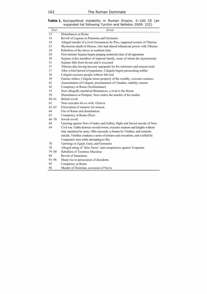
The Roman Dominate 162
Table 1. Sociopolitical instability in Roman Empire, 0–100 CE (an expanded list following Turchin and Nefedov 2009: 222)
Year Event 15 Disturbances at Rome 16 Revolt of Legions in Pannonia and Germania 19 Alleged murder of a rival Germanicus by Piso, supposed acolyte of Tiberius 23 Mysterious death of Drusus, who had shared tribunician power with Tiberius 24 Rebellion of the slaves in southern Italy 29 First minister Sejanus begins purging senatorial class of all opponents 30 Sejanus exiles members of imperial family, some of whom die mysteriously 31 Sejanus falls from favour and is executed 37 Tiberius dies having become unpopular for his informers and treason trials 37 After a brief period of popularity, Caligula begins persecuting nobles 38 Caligula executes people without full trial 39 Famine strikes, Caligula seizes property of the wealthy, executes senators 41 Assassination of Caligula; proclamation of Claudius, stability returns 42 Conspiracy at Rome (Scribonianus) 55 Nero allegedly murdered Britannicus, a rival to the throne 59 Disturbances at Pompeii, Nero orders the murder of his mother 60–61 British revolt 62 Nero executes his ex-wife, Octavia 62–63 Persecution of senators for treason 64 Fire of Rome and disturbances 65 Conspiracy at Rome (Piso) 66–70 Jewish revolt 68 Uprising against Nero (Vindex and Galba), flight and forced suicide of Nero 69 Civil war. Galba destroys several towns, executes senators and knights without
trial, murdered by army, Otho succeeds, is beaten by Vitellius, and commits suicide, Vitellius conducts a series of tortures and executions, and is killed by Vespasian's men while attempting to flee
70 Uprisings in Egypt, Gaul, and Germania 70 Alleged string of ‘false Neros’ and conspiracies against Vespasian 79–80 Rebellion of Terentius Maximus 89 Revolt of Saturninus 93–96 Sharp rise in persecution of dissidents 95 Conspiracy at Rome 96 Murder of Domitian, accession of Nerva
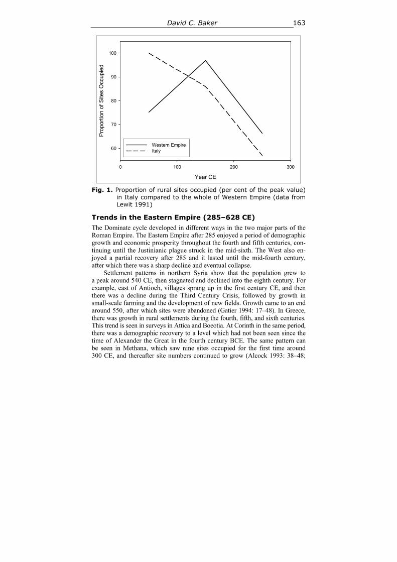
David C. Baker 163
Fig. 1. Proportion of rural sites occupied (per cent of the peak value)
in Italy compared to the whole of Western Empire (data from Lewit 1991)
Trends in the Eastern Empire (285–628 CE) The Dominate cycle developed in different ways in the two major parts of the Roman Empire. The Eastern Empire after 285 enjoyed a period of demographic growth and economic prosperity throughout the fourth and fifth centuries, con-tinuing until the Justinianic plague struck in the mid-sixth. The West also en-joyed a partial recovery after 285 and it lasted until the mid-fourth century, after which there was a sharp decline and eventual collapse.
Settlement patterns in northern Syria show that the population grew to a peak around 540 CE, then stagnated and declined into the eighth century. For example, east of Antioch, villages sprang up in the first century CE, and then there was a decline during the Third Century Crisis, followed by growth in small-scale farming and the development of new fields. Growth came to an end around 550, after which sites were abandoned (Gatier 1994: 17–48). In Greece, there was growth in rural settlements during the fourth, fifth, and sixth centuries. This trend is seen in surveys in Attica and Boeotia. At Corinth in the same period, there was a demographic recovery to a level which had not been seen since the time of Alexander the Great in the fourth century BCE. The same pattern can be seen in Methana, which saw nine sites occupied for the first time around 300 CE, and thereafter site numbers continued to grow (Alcock 1993: 38–48;
Year CE
0 100 200 300
Pro
port
ion
of S
ites
Occ
upie
d
60
70
80
90
100
Western EmpireItaly
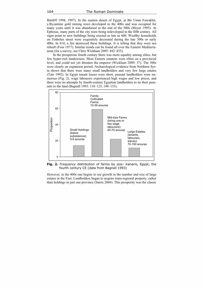
The Roman Dominate 164
Bintliff 1994, 1997). In the eastern desert of Egypt, at Bir Umm Fawakhir, a Byzantine gold mining town developed in the 400s and was occupied for many years until it was abandoned at the end of the 500s (Meyer 1995). At Ephesus, many parts of the city were being redeveloped in the fifth century. All signs point to new buildings being erected as late as 600. Wealthy households on Embolos street were exquisitely decorated during the late 300s or early 400s. In 614, a fire destroyed these buildings. It is telling that they were not rebuilt (Foss 1977). Similar trends can be found all over the Eastern Mediterra-nean (for a survey, see Chris Wickham 2005: 442–453).
In the prosperous fourth century there was more equality among elites, but few hyper-rich landowners. Most Eastern senators were elites on a provincial level, and could not yet threaten the emperor (Wickham 2009: 37). The 300s were clearly an expansion period. Archaeological evidence from Northern Syr-ia shows that there were many small landholders and very few large estates (Tate 1992). In Egypt tenant leases were short, peasant landholders were nu-merous (Fig. 2), wage labourers experienced high wages and low prices, and there were no attempts by fourth-century Egyptian landholders to tie their peas-ants to the land (Bagnall 1993: 110–123, 148–153).
Fig. 2. Frequency distribution of farms by size: Kanaris, Egypt, the
fourth century CE (data from Bagnall 1993)
However, in the 400s one begins to see growth in the number and size of large estates in the East. Landholders began to acquire trans-regional property, rather than holdings in just one province (Sarris 2004). This prosperity was the classic
Pro
por
tion
0
20
40
60
80
Small Holdings (below subsistence): 0-9 arouras
Family Cultivated Farms: 10-39 arouras
Mid-size Farms(hiring one or two wage labourers): 40-70 arouras
Large Estates(tenants, labourers, slaves): 70-150 arouras
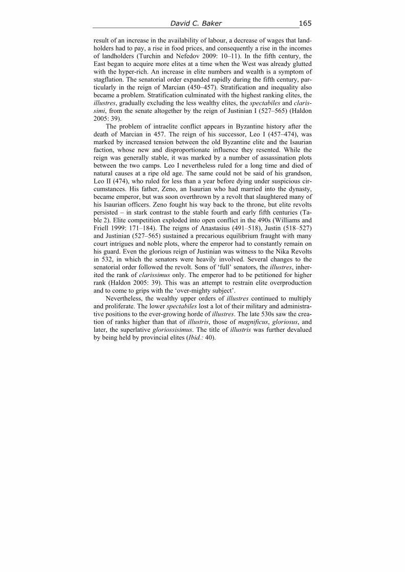
David C. Baker 165
result of an increase in the availability of labour, a decrease of wages that land-holders had to pay, a rise in food prices, and consequently a rise in the incomes of landholders (Turchin and Nefedov 2009: 10–11). In the fifth century, the East began to acquire more elites at a time when the West was already glutted with the hyper-rich. An increase in elite numbers and wealth is a symptom of stagflation. The senatorial order expanded rapidly during the fifth century, par-ticularly in the reign of Marcian (450–457). Stratification and inequality also became a problem. Stratification culminated with the highest ranking elites, the illustres, gradually excluding the less wealthy elites, the spectabiles and claris-simi, from the senate altogether by the reign of Justinian I (527–565) (Haldon 2005: 39).
The problem of intraelite conflict appears in Byzantine history after the death of Marcian in 457. The reign of his successor, Leo I (457–474), was marked by increased tension between the old Byzantine elite and the Isaurian faction, whose new and disproportionate influence they resented. While the reign was generally stable, it was marked by a number of assassination plots between the two camps. Leo I nevertheless ruled for a long time and died of natural causes at a ripe old age. The same could not be said of his grandson, Leo II (474), who ruled for less than a year before dying under suspicious cir-cumstances. His father, Zeno, an Isaurian who had married into the dynasty, became emperor, but was soon overthrown by a revolt that slaughtered many of his Isaurian officers. Zeno fought his way back to the throne, but elite revolts persisted – in stark contrast to the stable fourth and early fifth centuries (Ta-ble 2). Elite competition exploded into open conflict in the 490s (Williams and Friell 1999: 171–184). The reigns of Anastasius (491–518), Justin (518–527) and Justinian (527–565) sustained a precarious equilibrium fraught with many court intrigues and noble plots, where the emperor had to constantly remain on his guard. Even the glorious reign of Justinian was witness to the Nika Revolts in 532, in which the senators were heavily involved. Several changes to the senatorial order followed the revolt. Sons of ‘full’ senators, the illustres, inher-ited the rank of clarissimus only. The emperor had to be petitioned for higher rank (Haldon 2005: 39). This was an attempt to restrain elite overproduction and to come to grips with the ‘over-mighty subject’.
Nevertheless, the wealthy upper orders of illustres continued to multiply and proliferate. The lower spectabiles lost a lot of their military and administra-tive positions to the ever-growing horde of illustres. The late 530s saw the crea-tion of ranks higher than that of illustris, those of magnificus, gloriosus, and later, the superlative gloriossisimus. The title of illustris was further devalued by being held by provincial elites (Ibid.: 40).
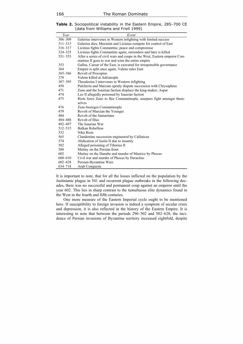
The Roman Dominate 166
Table 2. Sociopolitical instability in the Eastern Empire, 285–700 CE (data from Williams and Friell 1999)
Year Event 306–309 Galerius intervenes in Western infighting with limited success 311–313 Galerius dies, Maximin and Licinius compete for control of East 316–317 Licinius fights Constantine, peace and compromise 324–325 Licinius fights Constantine again, surrenders and later is killed 351–353 After a series of civil wars and coups in the West, Eastern emperor Con-
stantius II goes to war and wins the entire empire 353 Gallus, Caesar of the East, is executed for irresponsible governance 364 Empire is split once again, Valens rules East 365–366 Revolt of Procopius 378 Valens killed at Adrianople 387–395 Theodosius I intervenes in Western infighting 450 Pulcheria and Marcian openly dispute succession with Chrysaphius 471 Zeno and the Isaurian faction displace the king-maker, Aspar 474 Leo II allegedly poisoned by Isaurian faction 475 Riots force Zeno to flee Constantinople, usurpers fight amongst them-
selves 476 Zeno besieges Constantinople 479 Revolt of Marcian the Younger 484 Revolt of the Samaritans 484–488 Revolt of Illus 492–497 The Isaurian War 512–515 Balkan Rebellion 532 Nika Riots 565 Clandestine succession engineered by Callinicus 574 Abdication of Justin II due to insanity 582 Alleged poisoning of Tiberius II 588 Mutiny on the Persian front 602 Mutiny on the Danube and murder of Maurice by Phocas 608–610 Civil war and murder of Phocas by Heraclius 602–628 Persian-Byzantine Wars 634–718 Arab Conquests
It is important to note, that for all the losses inflicted on the population by the Justinianic plague in 541 and recurrent plague outbreaks in the following dec-ades, there was no successful and permanent coup against an emperor until the year 602. This lies in sharp contrast to the tumultuous elite dynamics found in the West in the fourth and fifth centuries.
One more measure of the Eastern Imperial cycle ought to be mentioned here. If susceptibility to foreign invasion is indeed a symptom of secular crisis and depression, it is also reflected in the history of the Eastern Empire. It is interesting to note that between the periods 296–502 and 502–628, the inci-dence of Persian invasions of Byzantine territory increased eightfold, despite
David C. Baker 167
the fact that the former period was nearly twice as long as the latter (Fig. 3). Afterward both the Eastern Empire and Persia collapsed from exhaustion and were overwhelmed by the Arab Conquests that soon burst upon the East.
Fig. 3. Persian incursions into Byzantine territory (data from Lee 1993)
One might ask whether the defeat in the Battle of Adrianople in 378, in which the Eastern emperor Valens was defeated and killed by the Goths, provides a counter-example. The incident is often treated as a milestone in accounts of the decline of the Roman Empire. Yet the year 378 falls within the Eastern ex-pansion phase. A simple explanation is that secular cycles do not dictate the outcome of individual battles, which are determined by a tangled web of vari-ables: tactics, supply, numerical strength, weather, topography, and countless others. The military defeat in 378 did not signal the secular decline of the East-ern Empire. It is testament to the high social cohesion of the region that after the Battle of Adrianople, despite the death of an emperor, Gothic forces were unable to take Constantinople, or indeed even the nearest town (Ward-Perkins 2005: 35).
In general, it appears that the Eastern Empire from 285–700 experienced a secular cycle that fits well with the basic model (except for its length – ap-proximately 400 years). To summarise, there was expansion in the fourth cen-tury, stagflation beginning somewhere in the fifth century, a crisis after the mid-sixth century, and depression in the upheavals of the seventh.
Year CE
200 250 300 350 400 450 500 550 600 650
Num
ber
of I
ncu
rsio
ns
pe
r H
alf-
Cen
tury
0
2
4
6
8
10
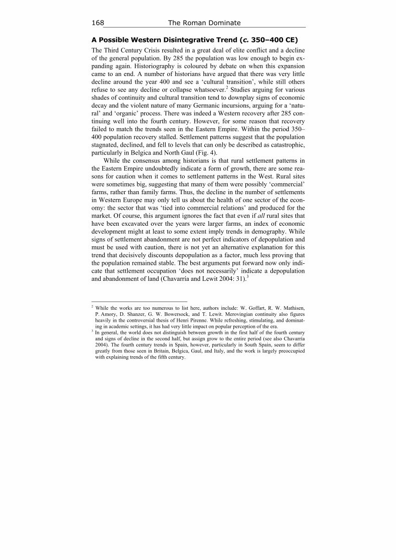
The Roman Dominate 168
A Possible Western Disintegrative Trend (c. 350–400 CE)
The Third Century Crisis resulted in a great deal of elite conflict and a decline of the general population. By 285 the population was low enough to begin ex-panding again. Historiography is coloured by debate on when this expansion came to an end. A number of historians have argued that there was very little decline around the year 400 and see a ‘cultural transition’, while still others refuse to see any decline or collapse whatsoever.2 Studies arguing for various shades of continuity and cultural transition tend to downplay signs of economic decay and the violent nature of many Germanic incursions, arguing for a ‘natu-ral’ and ‘organic’ process. There was indeed a Western recovery after 285 con-tinuing well into the fourth century. However, for some reason that recovery failed to match the trends seen in the Eastern Empire. Within the period 350–400 population recovery stalled. Settlement patterns suggest that the population stagnated, declined, and fell to levels that can only be described as catastrophic, particularly in Belgica and North Gaul (Fig. 4).
While the consensus among historians is that rural settlement patterns in the Eastern Empire undoubtedly indicate a form of growth, there are some rea-sons for caution when it comes to settlement patterns in the West. Rural sites were sometimes big, suggesting that many of them were possibly ‘commercial’ farms, rather than family farms. Thus, the decline in the number of settlements in Western Europe may only tell us about the health of one sector of the econ-omy: the sector that was ‘tied into commercial relations’ and produced for the market. Of course, this argument ignores the fact that even if all rural sites that have been excavated over the years were larger farms, an index of economic development might at least to some extent imply trends in demography. While signs of settlement abandonment are not perfect indicators of depopulation and must be used with caution, there is not yet an alternative explanation for this trend that decisively discounts depopulation as a factor, much less proving that the population remained stable. The best arguments put forward now only indi-cate that settlement occupation ‘does not necessarily’ indicate a depopulation and abandonment of land (Chavarría and Lewit 2004: 31).3
2 While the works are too numerous to list here, authors include: W. Goffart, R. W. Mathisen,
P. Amory, D. Shanzer, G. W. Bowersock, and T. Lewit. Merovingian continuity also figures heavily in the controversial thesis of Henri Pirenne. While refreshing, stimulating, and dominat-ing in academic settings, it has had very little impact on popular perception of the era.
3 In general, the world does not distinguish between growth in the first half of the fourth century and signs of decline in the second half, but assign grow to the entire period (see also Chavarría 2004). The fourth century trends in Spain, however, particularly in South Spain, seem to differ greatly from those seen in Britain, Belgica, Gaul, and Italy, and the work is largely preoccupied with explaining trends of the fifth century.
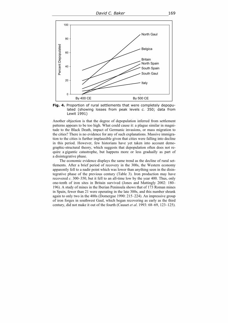
David C. Baker 169
Fig. 4. Proportion of rural settlements that were completely depopu-
lated (showing losses from peak levels c. 350; data from Lewit 1991)
Another objection is that the degree of depopulation inferred from settlement patterns appears to be too high. What could cause it: a plague similar in magni-tude to the Black Death, impact of Germanic invasions, or mass migration to the cities? There is no evidence for any of such explanations. Massive immigra-tion to the cities is further implausible given that cities were falling into decline in this period. However, few historians have yet taken into account demo-graphic-structural theory, which suggests that depopulation often does not re-quire a gigantic catastrophe, but happens more or less gradually as part of a disintegrative phase.
The economic evidence displays the same trend as the decline of rural set-tlements. After a brief period of recovery in the 300s, the Western economy apparently fell to a nadir point which was lower than anything seen in the disin-tegrative phase of the previous century (Table 3). Iron production may have recovered c. 300–350, but it fell to an all-time low by the year 400. Thus, only one-tenth of iron sites in Britain survived (Jones and Mattingly 2002: 180–196). A study of mines in the Iberian Peninsula shows that of 173 Roman mines in Spain, fewer than 21 were operating in the late 300s, and this number shrank again to only two in the 400s (Domergue 1990: 215–224). An impressive group of iron forges in southwest Gaul, which began recovering as early as the third century, did not make it out of the fourth (Cauuet et al. 1993: 68–69, 123–125).
Per
cent
Dep
opul
ated
0
20
40
60
80
100
By 400 CE By 500 CE
Italy
South Gaul
North SpainBritain
Belgica
North Gaul
South Spain
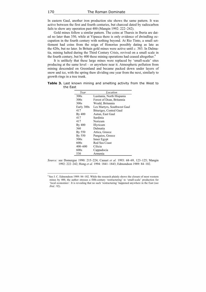
The Roman Dominate 170
In eastern Gaul, another iron production site shows the same pattern. It was active between the first and fourth centuries, but charcoal dated by radiocarbon fails to show any operation past 400 (Mangin 1992: 222–242).
Gold mines follow a similar pattern. The coins at Tharsis in Iberia are dat-ed no later than 350, while at Vipasca there is only evidence of dwindling oc-cupation in the fourth century with nothing beyond. At Rio Tinto, a small set-tlement had coins from the reign of Honorius possibly dating as late as the 420s, but no later. In Britain gold mines were active until c. 383. In Dalma-tia, mining halted during the Third Century Crisis, revived on a small scale in the fourth century, but by 400 these mining operations had ceased altogether.4
It is unlikely that these large mines were replaced by ‘small-scale’ sites producing at the same level – or anywhere near it. Atmospheric pollution from mining descended on Greenland and became packed down under layers of snow and ice, with the spring thaw dividing one year from the next, similarly to growth rings in a tree trunk.
Table 3. Last known mining and smelting activity from the West to the East
Year Location 300s Lusitania, North Hispania 300s Forest of Dean, Britannia 300s Weald, Britannia Early 300s Les Martyrs, Southwest Gaul 417 Bituriges, Central Gaul By 400 Autun, East Gaul 417 Sardinia 417 Noricum By 400 Illyricum 360 Dalmatia By 550 Attica, Greece By 550 Pangaios, Greece 500s Inner Egypt 600s Red Sea Coast 400–600 Cilicia 600s Cappadocia 530 Armenia
Source: see Domergue 1990: 215–224; Cauuet et al. 1993: 68–69, 123–125; Mangin 1992: 222–242; Hong et al. 1994: 1841–1843; Edmondson 1989: 84–102.
4 See J. C. Edmondson 1989: 84–102. While the research plainly shows the closure of most western
mines by 400, the author stresses a fifth-century ‘restructuring’ to ‘small-scale’ production for ‘local economies’. It is revealing that no such ‘restructuring’ happened anywhere in the East (see Ibid.: 92).
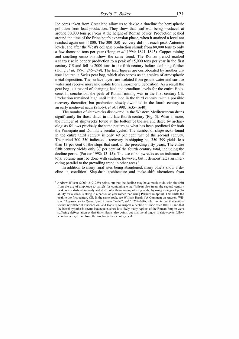
David C. Baker 171
Ice cores taken from Greenland allow us to devise a timeline for hemispheric pollution from lead production. They show that lead was being produced at around 80,000 tons per year at the height of Roman power. Production peaked around the time of the Principate's expansion phase, when it attained a level not reached again until 1800. The 300–350 recovery did not reach peak Antonine levels, and after the West's collapse production shrunk from 80,000 tons to only a few thousand tons per year (Hong et al. 1994: 1841–1843). Copper mining and smelting emissions show the same trend. The Roman period marked a sharp rise in copper production to a peak of 15,000 tons per year in the first century CE and fell to 2000 tons in the fifth century before declining further (Hong et al. 1996: 246–249). The lead figures are corroborated by another un-usual source, a Swiss peat bog, which also serves as an archive of atmospheric metal deposition. The surface layers are isolated from groundwater and surface water and receive inorganic solids from atmospheric deposition. As a result the peat bog is a record of changing lead and scandium levels for the entire Holo-cene. In conclusion, the peak of Roman mining was in the first century CE. Production remained high until it declined in the third century, with a possible recovery thereafter, but production slowly dwindled in the fourth century to an early medieval nadir (Shotyk et al. 1998: 1635–1640).
The number of shipwrecks discovered in the Western Mediterranean drops significantly for those dated in the late fourth century (Fig. 5). What is more, the number of shipwrecks found at the bottom of the sea and dated by archae-ologists follows precisely the same pattern as what has been predicted for both the Principate and Dominate secular cycles. The number of shipwrecks found in the entire third century is only 49 per cent that of the second century. The period 300–350 indicates a recovery in shipping but 350–399 yields less than 13 per cent of the ships that sunk in the preceding fifty years. The entire fifth century yields only 37 per cent of the fourth century total, including the decline period (Parker 1992: 13–15). The use of shipwrecks as an indicator of total volume must be done with caution, however, but it demonstrates an inter-esting parallel to the prevailing trend in other areas.5
In addition to many rural sites being abandoned, many others show a de-cline in condition. Slap-dash architecture and make-shift alterations from
5 Andrew Wilson (2009: 219–229) points out that the decline may have much to do with the shift
from the use of amphorae to barrels for containing wine. Wilson also treats the second century peak as a statistical anomaly and distributes them among other periods, by using a range of prob-ability for a wreck sinking in a particular year rather than using Parker's midpoint. This shifts the peak to the first century CE. In the same book, see William Harris (‘A Comment on Andrew Wil-son: “Approaches to Quantifying Roman Trade”’, Ibid.: 259–260), who points out that neither textual nor material evidence on land leads us to suspect a decline of trade after 100 CE and that the barrel hypothesis seems inadequate, since it is likely many regions of the Roman Empire were suffering deforestation at that time. Harris also points out that metal ingots in shipwrecks follow a contradictory trend from the amphorae first century peak.
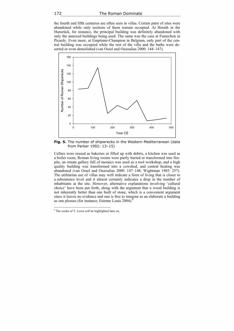
The Roman Dominate 172
the fourth and fifth centuries are often seen in villas. Certain parts of sites were abandoned while only sections of them remain occupied. At Horath in the Hunsrück, for instance, the principal building was definitely abandoned with only the annexed buildings being used. The same was the case at Famechon in Picardy. Even more, at Emptinne-Champion in Belgium, only part of the cen-tral building was occupied while the rest of the villa and the baths were de-serted or even demolished (van Ossel and Ouzoulias 2000: 144–147).
Fig. 5. The number of shipwrecks in the Western Mediterranean (data
from Parker 1992: 13–15)
Cellars were reused as bakeries or filled up with debris, a kitchen was used as a boiler room, Roman living rooms were partly buried or transformed into fire-pits, an ornate gallery full of mosaics was used as a tool workshop, and a high quality building was transformed into a cowshed, and central heating was abandoned (van Ossel and Ouzoulias 2000: 147–148; Wightman 1985: 257). The utilitarian use of villas may well indicate a form of living that is closer to a subsistence level and it almost certainly indicates a drop in the number of inhabitants at the site. However, alternative explanations involving ‘cultural choice’ have been put forth, along with the argument that a wood building is not inherently better than one built of stone, which is a convenient argument since it leaves no evidence and one is free to imagine as an elaborate a building as one pleases (for instance, Etienne Louis 2004).6
6 The works of T. Lewit will be highlighted later on.
Year CE
0 100 200 300 400 500
Num
ber
of R
oman
Shi
pwre
cks
0
20
40
60
80
100
120
140
160
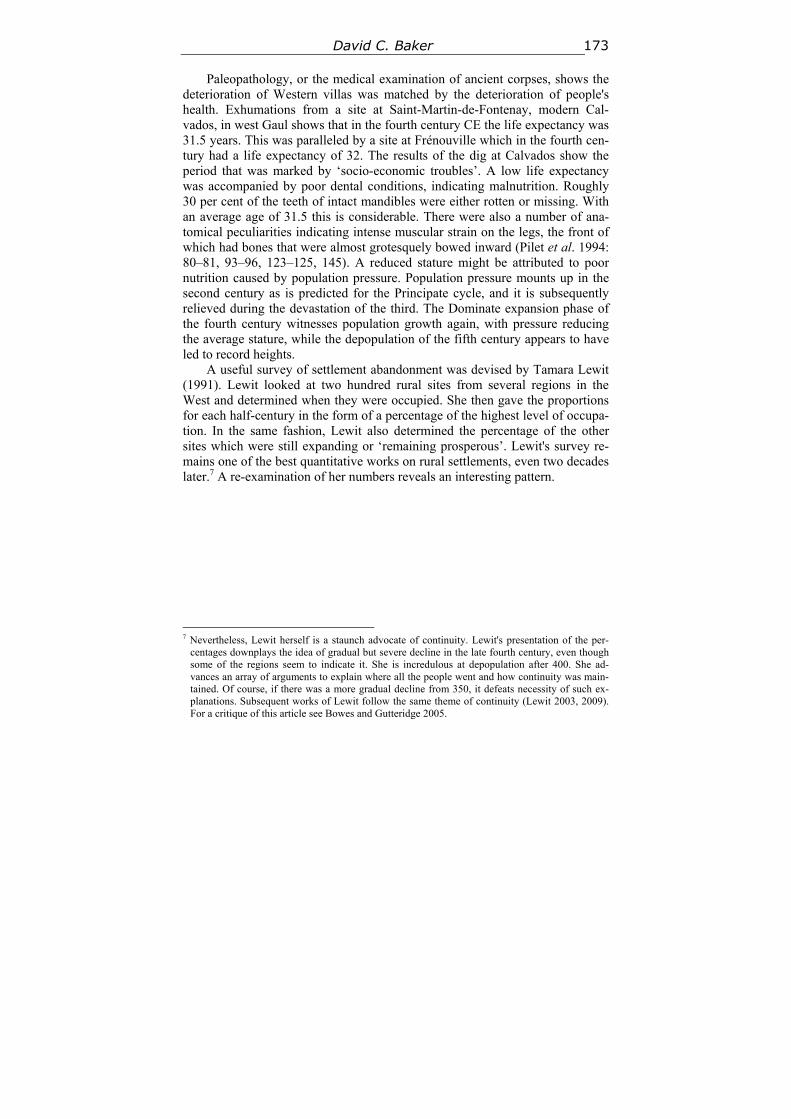
David C. Baker 173
Paleopathology, or the medical examination of ancient corpses, shows the deterioration of Western villas was matched by the deterioration of people's health. Exhumations from a site at Saint-Martin-de-Fontenay, modern Cal-vados, in west Gaul shows that in the fourth century CE the life expectancy was 31.5 years. This was paralleled by a site at Frénouville which in the fourth cen-tury had a life expectancy of 32. The results of the dig at Calvados show the period that was marked by ‘socio-economic troubles’. A low life expectancy was accompanied by poor dental conditions, indicating malnutrition. Roughly 30 per cent of the teeth of intact mandibles were either rotten or missing. With an average age of 31.5 this is considerable. There were also a number of ana-tomical peculiarities indicating intense muscular strain on the legs, the front of which had bones that were almost grotesquely bowed inward (Pilet et al. 1994: 80–81, 93–96, 123–125, 145). A reduced stature might be attributed to poor nutrition caused by population pressure. Population pressure mounts up in the second century as is predicted for the Principate cycle, and it is subsequently relieved during the devastation of the third. The Dominate expansion phase of the fourth century witnesses population growth again, with pressure reducing the average stature, while the depopulation of the fifth century appears to have led to record heights.
A useful survey of settlement abandonment was devised by Tamara Lewit (1991). Lewit looked at two hundred rural sites from several regions in the West and determined when they were occupied. She then gave the proportions for each half-century in the form of a percentage of the highest level of occupa-tion. In the same fashion, Lewit also determined the percentage of the other sites which were still expanding or ‘remaining prosperous’. Lewit's survey re-mains one of the best quantitative works on rural settlements, even two decades later.7 A re-examination of her numbers reveals an interesting pattern.
7 Nevertheless, Lewit herself is a staunch advocate of continuity. Lewit's presentation of the per-
centages downplays the idea of gradual but severe decline in the late fourth century, even though some of the regions seem to indicate it. She is incredulous at depopulation after 400. She ad-vances an array of arguments to explain where all the people went and how continuity was main-tained. Of course, if there was a more gradual decline from 350, it defeats necessity of such ex-planations. Subsequent works of Lewit follow the same theme of continuity (Lewit 2003, 2009). For a critique of this article see Bowes and Gutteridge 2005.
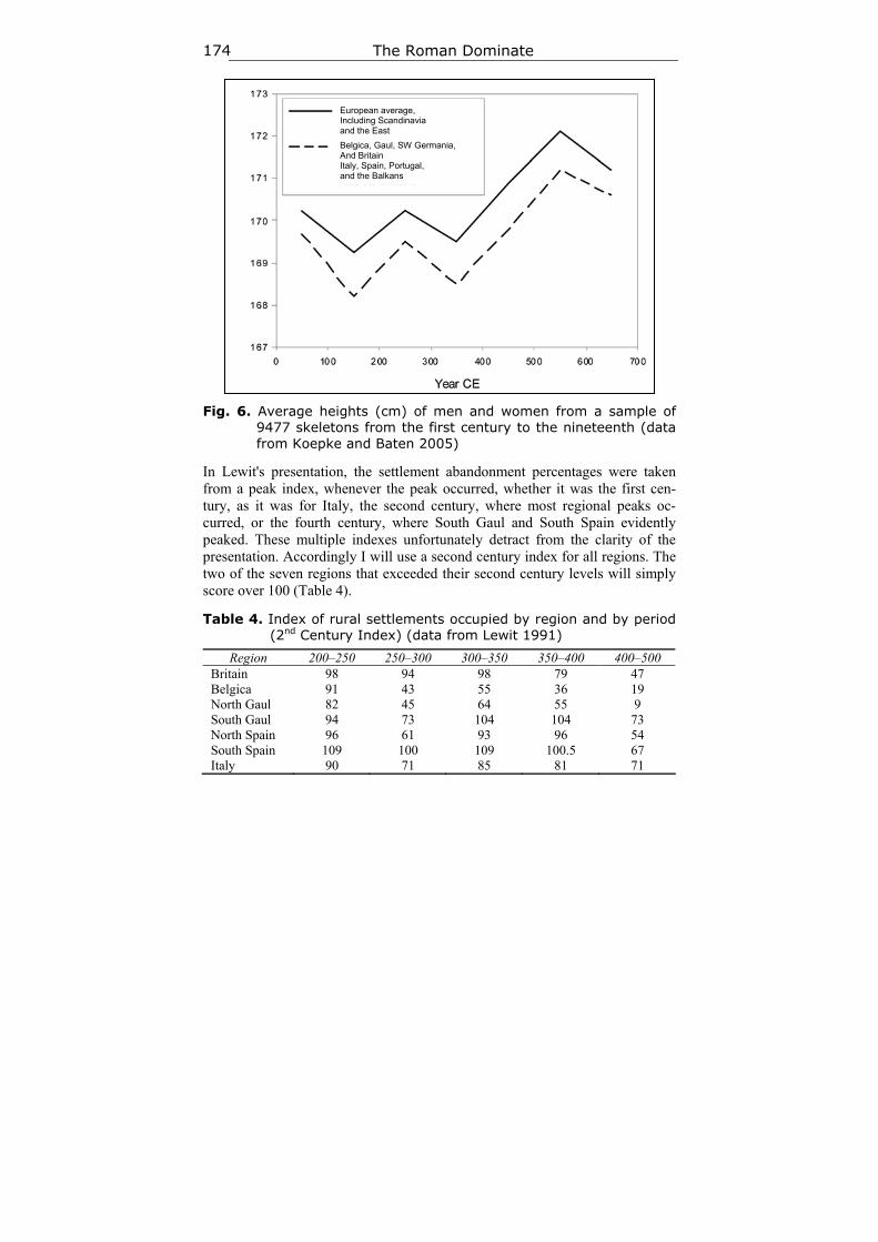
The Roman Dominate 174
Fig. 6. Average heights (cm) of men and women from a sample of 9477 skeletons from the first century to the nineteenth (data from Koepke and Baten 2005)
In Lewit's presentation, the settlement abandonment percentages were taken from a peak index, whenever the peak occurred, whether it was the first cen-tury, as it was for Italy, the second century, where most regional peaks oc-curred, or the fourth century, where South Gaul and South Spain evidently peaked. These multiple indexes unfortunately detract from the clarity of the presentation. Accordingly I will use a second century index for all regions. The two of the seven regions that exceeded their second century levels will simply score over 100 (Table 4).
Table 4. Index of rural settlements occupied by region and by period (2nd Century Index) (data from Lewit 1991)
Region 200–250 250–300 300–350 350–400 400–500 Britain 98 94 98 79 47 Belgica 91 43 55 36 19 North Gaul 82 45 64 55 9 South Gaul 94 73 104 104 73 North Spain 96 61 93 96 54 South Spain 109 100 109 100.5 67 Italy 90 71 85 81 71
European average, Including Scandinavia and the East
Belgica, Gaul, SW Germania, And Britain Italy, Spain, Portugal, and the Balkans
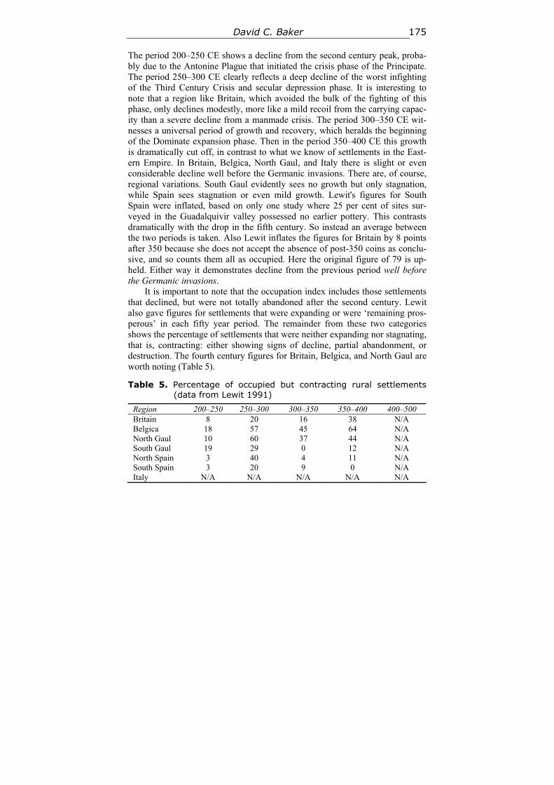
David C. Baker 175
The period 200–250 CE shows a decline from the second century peak, proba-bly due to the Antonine Plague that initiated the crisis phase of the Principate. The period 250–300 CE clearly reflects a deep decline of the worst infighting of the Third Century Crisis and secular depression phase. It is interesting to note that a region like Britain, which avoided the bulk of the fighting of this phase, only declines modestly, more like a mild recoil from the carrying capac-ity than a severe decline from a manmade crisis. The period 300–350 CE wit-nesses a universal period of growth and recovery, which heralds the beginning of the Dominate expansion phase. Then in the period 350–400 CE this growth is dramatically cut off, in contrast to what we know of settlements in the East-ern Empire. In Britain, Belgica, North Gaul, and Italy there is slight or even considerable decline well before the Germanic invasions. There are, of course, regional variations. South Gaul evidently sees no growth but only stagnation, while Spain sees stagnation or even mild growth. Lewit's figures for South Spain were inflated, based on only one study where 25 per cent of sites sur-veyed in the Guadalquivir valley possessed no earlier pottery. This contrasts dramatically with the drop in the fifth century. So instead an average between the two periods is taken. Also Lewit inflates the figures for Britain by 8 points after 350 because she does not accept the absence of post-350 coins as conclu-sive, and so counts them all as occupied. Here the original figure of 79 is up-held. Either way it demonstrates decline from the previous period well before the Germanic invasions.
It is important to note that the occupation index includes those settlements that declined, but were not totally abandoned after the second century. Lewit also gave figures for settlements that were expanding or were ‘remaining pros-perous’ in each fifty year period. The remainder from these two categories shows the percentage of settlements that were neither expanding nor stagnating, that is, contracting: either showing signs of decline, partial abandonment, or destruction. The fourth century figures for Britain, Belgica, and North Gaul are worth noting (Table 5).
Table 5. Percentage of occupied but contracting rural settlements (data from Lewit 1991)
Region 200–250 250–300 300–350 350–400 400–500 Britain 8 20 16 38 N/A Belgica 18 57 45 64 N/A North Gaul 10 60 37 44 N/A South Gaul 19 29 0 12 N/A North Spain 3 40 4 11 N/A South Spain 3 20 9 0 N/A Italy N/A N/A N/A N/A N/A
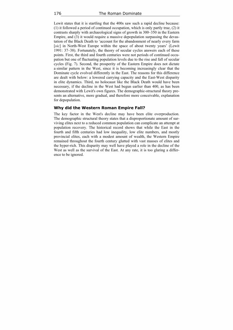
The Roman Dominate 176
Lewit states that it is startling that the 400s saw such a rapid decline because: (1) it followed a period of continued occupation, which is only partly true, (2) it contrasts sharply with archaeological signs of growth in 300–350 in the Eastern Empire, and (3) it would require a massive depopulation surpassing the devas-tation of the Black Death to ‘account for the abandonment of nearly every farm [sic] in North-West Europe within the space of about twenty years’ (Lewit 1991: 37–38). Fortunately, the theory of secular cycles answers each of these points. First, the third and fourth centuries were not periods of continued occu-pation but one of fluctuating population levels due to the rise and fall of secular cycles (Fig. 7). Second, the prosperity of the Eastern Empire does not dictate a similar pattern in the West, since it is becoming increasingly clear that the Dominate cycle evolved differently in the East. The reasons for this difference are dealt with below: a lowered carrying capacity and the East-West disparity in elite dynamics. Third, no holocaust like the Black Death would have been necessary, if the decline in the West had begun earlier than 400, as has been demonstrated with Lewit's own figures. The demographic-structural theory pre-sents an alternative, more gradual, and therefore more conceivable, explanation for depopulation.
Why did the Western Roman Empire Fall?
The key factor in the West's decline may have been elite overproduction. The demographic structural theory states that a disproportionate amount of sur-viving elites next to a reduced common population can complicate an attempt at population recovery. The historical record shows that while the East in the fourth and fifth centuries had low inequality, low elite numbers, and mostly provincial elites, each with a modest amount of wealth, the Western Empire remained throughout the fourth century glutted with vast masses of elites and the hyper-rich. This disparity may well have played a role in the decline of the West as well as the survival of the East. At any rate, it is too glaring a differ-ence to be ignored.
David C. Baker 177
Fig. 7. Dynamics of rural settlement occupation for each major region
in Western Europe (data from Lewit 1991)
Firstly, we do know that the early fourth century saw an impressive boom in large villa estates, which might indicate the concentration of land into the hands of the few. The standard explanation, the retreat of the aristocracy to the coun-tryside, is unlikely. Instead this pattern could be explained by an early fourth century stagflation dynamic (Chavarría and Lewit 2004: 26–29). We also know something about the immense inequality gap between elite and commoner at this time. The Late Antique historian, Olympiodorus (c. 380 – ? CE), tells us that the richest senators of the West had yearly incomes of four thousand pounds of gold a year, while mid-level senators had around one thousand pounds a year. A commoner, by comparison, could scratch together perhaps five solidi in a year's toil, or less than one-fourteenth of a pound of gold.8 It is interesting to note this disparity of wealth outstrips inequality ratios for the stagflation period of the Principate and also the most extravagant periods of later French or English history. Additionally, wealthy Roman nobleman Quin-tus Aurelius Symmachus (c. 340–405) spent around two thousand pounds of gold at one go, on the celebration of his son's praetorship, by personally financ-ing the games in Rome. This ritual was common among the Roman elite in Late
8 For senatorial incomes see Olympiodorus, in Photius, Bibliotheca (1920), frag. 44. For the esti-
mate for a peasant's income see Ward, Heichelheim, and Yeo 1999: 446. This astounding inequal-ity ratio and disparity of wealth is also dealt with in Turchin 2006: 160–161.
Year CE
200 250 300 350 400 450 500
Occ
upat
ion
Inde
x
40
60
80
100
ItalyGaulSpainBritain
The Roman Dominate 178
Antiquity whenever a family member achieved such a distinction, and it was a social obligation to match or even surpass the displays of splendour and con-sumption of a rival family (Olympiodorus 1920).
St. Melania the Younger (c. 383–439) came from a foremost senatorial family. She married her cousin, Pinian, around 399. After a miscarriage of two children they found religion, took vows of celibacy, and gave up their worldly possessions. Pinian is said to have held an annual income of 120,000 ‘pieces’ of gold, on top of his wife's income of about the same amount (Gerontius 1984: 15). ‘Pieces of gold’ has in the past been interpreted as either pounds or solidi. If more realistically interpreted as solidi, that amounts to 1666 pounds annually, and that roughly equates with what Olympiodorus tells us about the average senatorial income. If multiplied by two, for it appears Melania held a compara-ble income separate of Pinian, the total income comes to around 3332 pounds of gold annually. This point has been debated among historians. Whether or not Melania and Pinian held a mid-level or a combined upper level senatorial in-come, it nevertheless appears that when they sold their lands, the sale temporar-ily caused panic and a fiscal crisis in the property market (Wickham 2005: 29). Apparently one of the estates sold by Melania in North Africa was larger than the nearest town, Thagaste, birthplace of St. Augustine (Gerontius 1984: 21). The presence of such trans-regional hyper-rich is certainly at variance with what one would typically expect to see of elite dynamics in a supposedly inte-grative period.
The paucity of sources from this period makes it next to be impossible to find similar quantitative data for the late fourth century. However, various writ-ten testimonies confirm the income figures of Olympiodorus and those for Melania the Younger. For instance, Ammianus Marcellinus (c. 325–390), a prominent imperial official and the principal historian of the period, came to Rome from Antioch and was disgusted with the decadence he saw. He writes of a certain number of idle and frivolous senators, who gorged themselves with food at luxurious banquets. They spent large sums of money on exotic dancers and prostitutes.
During a food shortage in Rome, all foreigners were expelled from the city, while the senators lobbied for three thousand dancers and ladies of negotiable virtue to remain. The Roman elite gave hugely expensive shows featuring dra-matic actors. The elite were given to the habit of conspicuous consumption, and clothed themselves in effete, elaborately designed silk and dyed robes. They lined the streets with gold plated statues of themselves and their ancestors. At the baths, they were attended by as many as fifty servants. Now, some histo-rians have suggested that Ammianus was just ‘rephrasing late antique com-monplaces’ but that is precisely the point. They were commonplaces for a rea-son. Ammianus would hardly need to set up a stock figure to decry elite con-sumption unless there was something to decry. Furthermore, it is worthwhile
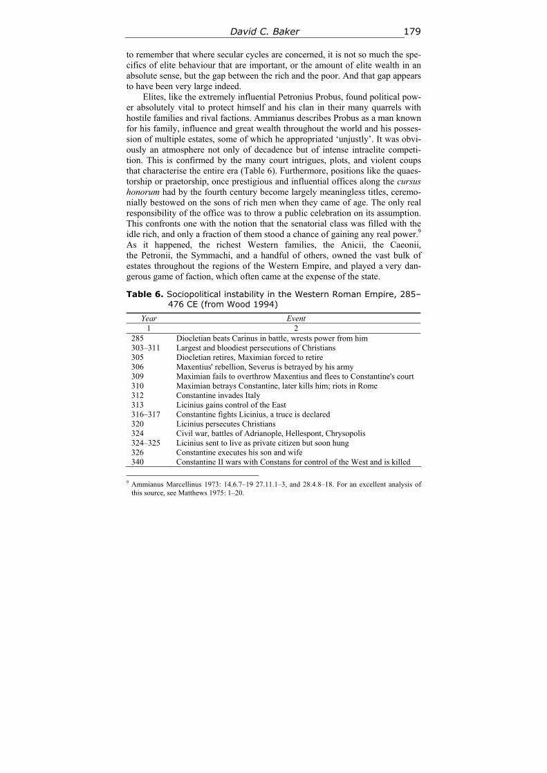
David C. Baker 179
to remember that where secular cycles are concerned, it is not so much the spe-cifics of elite behaviour that are important, or the amount of elite wealth in an absolute sense, but the gap between the rich and the poor. And that gap appears to have been very large indeed.
Elites, like the extremely influential Petronius Probus, found political pow-er absolutely vital to protect himself and his clan in their many quarrels with hostile families and rival factions. Ammianus describes Probus as a man known for his family, influence and great wealth throughout the world and his posses-sion of multiple estates, some of which he appropriated ‘unjustly’. It was obvi-ously an atmosphere not only of decadence but of intense intraelite competi-tion. This is confirmed by the many court intrigues, plots, and violent coups that characterise the entire era (Table 6). Furthermore, positions like the quaes-torship or praetorship, once prestigious and influential offices along the cursus honorum had by the fourth century become largely meaningless titles, ceremo-nially bestowed on the sons of rich men when they came of age. The only real responsibility of the office was to throw a public celebration on its assumption. This confronts one with the notion that the senatorial class was filled with the idle rich, and only a fraction of them stood a chance of gaining any real power.9 As it happened, the richest Western families, the Anicii, the Caeonii, the Petronii, the Symmachi, and a handful of others, owned the vast bulk of estates throughout the regions of the Western Empire, and played a very dan-gerous game of faction, which often came at the expense of the state.
Table 6. Sociopolitical instability in the Western Roman Empire, 285– 476 CE (from Wood 1994)
Year Event 1 2
285 Diocletian beats Carinus in battle, wrests power from him 303–311 Largest and bloodiest persecutions of Christians 305 Diocletian retires, Maximian forced to retire 306 Maxentius' rebellion, Severus is betrayed by his army 309 Maximian fails to overthrow Maxentius and flees to Constantine's court 310 Maximian betrays Constantine, later kills him; riots in Rome 312 Constantine invades Italy 313 Licinius gains control of the East 316–317 Constantine fights Licinius, a truce is declared 320 Licinius persecutes Christians 324 Civil war, battles of Adrianople, Hellespont, Chrysopolis 324–325 Licinius sent to live as private citizen but soon hung 326 Constantine executes his son and wife 340 Constantine II wars with Constans for control of the West and is killed
9 Ammianus Marcellinus 1973: 14.6.7–19 27.11.1–3, and 28.4.8–18. For an excellent analysis of
this source, see Matthews 1975: 1–20.
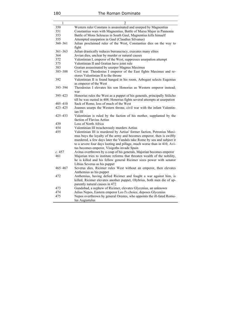
The Roman Dominate 180
1 2 350 Western ruler Constans is assassinated and usurped by Magnentius 351 Constantius wars with Magnentius, Battle of Mursa Major in Pannonia 353 Battle of Mons Seleucus in South Gaul, Magnentius kills himself 355 Attempted usurpation in Gaul (Claudius Silvanus) 360–361 Julian proclaimed ruler of the West, Constantius dies on the way to
fight 361–363 Julian drastically reduces bureaucracy, executes many elites 364 Jovian dies, unclear by murder or natural causes 372 Valentinian I, emperor of the West, suppresses usurpation attempt 375 Valentinian II and Gratian have joint rule 383 Gratian assassinated by usurper Magnus Maximus 383–388 Civil war. Theodosius I emperor of the East fights Maximus and re-
stores Valentinian II to the throne 392 Valentinian II is found hanged in his room, Arbogast selects Eugenius
as emperor of the West 393–394 Theodosius I elevates his son Honorius as Western emperor instead;
war 395–423 Honorius rules the West as a puppet of his generals, principally Stilicho
till he was ousted in 408; Honorius fights several attempts at usurpation 405–410 Sack of Rome, loss of much of the West 423–425 Joannes usurps the Western throne, civil war with the infant Valentin-
ian III 425–433 Valentinian is ruled by the faction of his mother, supplanted by the
faction of Flavius Aetius 439 Loss of North Africa 454 Valentinian III treacherously murders Aetius 455 Valentinian III is murdered by Aetius' former faction, Petronius Maxi-
mus buys the loyalty of the army and becomes emperor, then is swiftly murdered, a few days later the Vandals take Rome by sea and subject it to a severe four days looting and pillage, much worse than in 410, Avi-tus becomes emperor, Visigoths invade Spain
c. 457 Avitus overthrown by a coup of his generals, Majorian becomes emperor 461 Majorian tries to institute reforms that threaten wealth of the nobility,
he is killed and his fellow general Ricimer sizes power with senator Libius Severus as his puppet
465–467 Severus dies, Ricimer rules West without an emperor, then elevates Anthemius as his puppet
472 Anthemius, having defied Ricimer and fought a war against him, is killed, Ricimer elevates another puppet, Olybrius, both men die of ap-parently natural causes in 472
473 Gundobad, a nephew of Ricimer, elevates Glycenius, an unknown 474 Julius Nepos, Eastern emperor Leo I's choice, deposes Glycenius 475 Nepos overthrown by general Orestes, who appoints the ill-fated Romu-
lus Augustulus
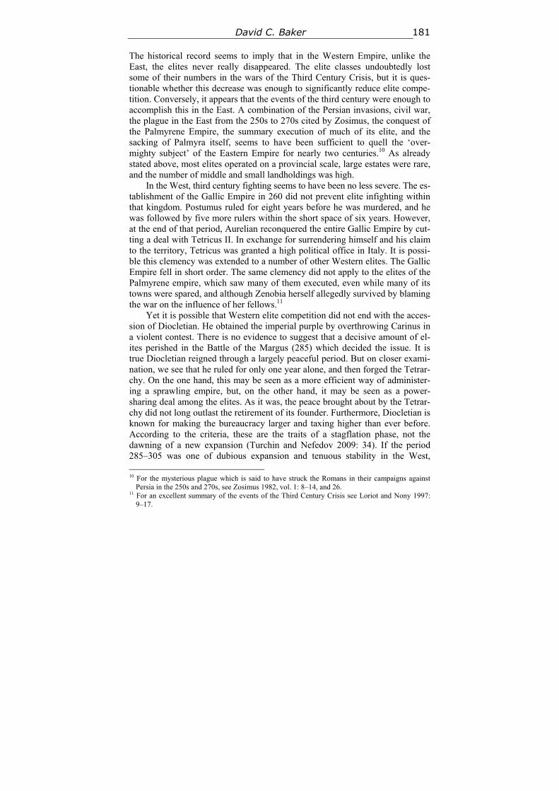
David C. Baker 181
The historical record seems to imply that in the Western Empire, unlike the East, the elites never really disappeared. The elite classes undoubtedly lost some of their numbers in the wars of the Third Century Crisis, but it is ques-tionable whether this decrease was enough to significantly reduce elite compe-tition. Conversely, it appears that the events of the third century were enough to accomplish this in the East. A combination of the Persian invasions, civil war, the plague in the East from the 250s to 270s cited by Zosimus, the conquest of the Palmyrene Empire, the summary execution of much of its elite, and the sacking of Palmyra itself, seems to have been sufficient to quell the ‘over-mighty subject’ of the Eastern Empire for nearly two centuries.10 As already stated above, most elites operated on a provincial scale, large estates were rare, and the number of middle and small landholdings was high.
In the West, third century fighting seems to have been no less severe. The es-tablishment of the Gallic Empire in 260 did not prevent elite infighting within that kingdom. Postumus ruled for eight years before he was murdered, and he was followed by five more rulers within the short space of six years. However, at the end of that period, Aurelian reconquered the entire Gallic Empire by cut-ting a deal with Tetricus II. In exchange for surrendering himself and his claim to the territory, Tetricus was granted a high political office in Italy. It is possi-ble this clemency was extended to a number of other Western elites. The Gallic Empire fell in short order. The same clemency did not apply to the elites of the Palmyrene empire, which saw many of them executed, even while many of its towns were spared, and although Zenobia herself allegedly survived by blaming the war on the influence of her fellows.11
Yet it is possible that Western elite competition did not end with the acces-sion of Diocletian. He obtained the imperial purple by overthrowing Carinus in a violent contest. There is no evidence to suggest that a decisive amount of el-ites perished in the Battle of the Margus (285) which decided the issue. It is true Diocletian reigned through a largely peaceful period. But on closer exami-nation, we see that he ruled for only one year alone, and then forged the Tetrar-chy. On the one hand, this may be seen as a more efficient way of administer-ing a sprawling empire, but, on the other hand, it may be seen as a power-sharing deal among the elites. As it was, the peace brought about by the Tetrar-chy did not long outlast the retirement of its founder. Furthermore, Diocletian is known for making the bureaucracy larger and taxing higher than ever before. According to the criteria, these are the traits of a stagflation phase, not the dawning of a new expansion (Turchin and Nefedov 2009: 34). If the period 285–305 was one of dubious expansion and tenuous stability in the West, 10 For the mysterious plague which is said to have struck the Romans in their campaigns against
Persia in the 250s and 270s, see Zosimus 1982, vol. 1: 8–14, and 26. 11 For an excellent summary of the events of the Third Century Crisis see Loriot and Nony 1997:
9–17.
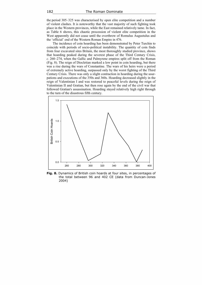
The Roman Dominate 182
the period 305–325 was characterised by open elite competition and a number of violent clashes. It is noteworthy that the vast majority of such fighting took place in the Western provinces, while the East remained relatively tame. In fact, as Table 6 shows, this chaotic procession of violent elite competition in the West apparently did not cease until the overthrow of Romulus Augustulus and the ‘official’ end of the Western Roman Empire in 476.
The incidence of coin hoarding has been demonstrated by Peter Turchin to coincide with periods of socio-political instability. The quantity of coin finds from four excavated sites Britain, the most thoroughly studied province, shows that hoarding peaked during the severest phase of the Third Century Crisis, c. 260–274, when the Gallic and Palmyrene empires split off from the Roman (Fig. 8). The reign of Diocletian marked a low point in coin hoarding, but there was a rise during the wars of Constantine. The wars of his heirs were a period of extremely active hoarding, surpassed only by the worst fighting of the Third Century Crisis. There was only a slight contraction in hoarding during the usur-pations and executions of the 350s and 360s. Hoarding decreased slightly in the reign of Valentinian I and was restored to peaceful levels during the reign of Valentinian II and Gratian, but then rose again by the end of the civil war that followed Gratian's assassination. Hoarding stayed relatively high right through to the turn of the disastrous fifth century.
Fig. 8. Dynamics of British coin hoards at four sites, in percentages of
the total between 96 and 402 CE (data from Duncan-Jones 2004)
260 280 300 320 340 360 380 400
Bri
tish
Coi
n H
oard
s
0.0
0.5
1.0
1.5
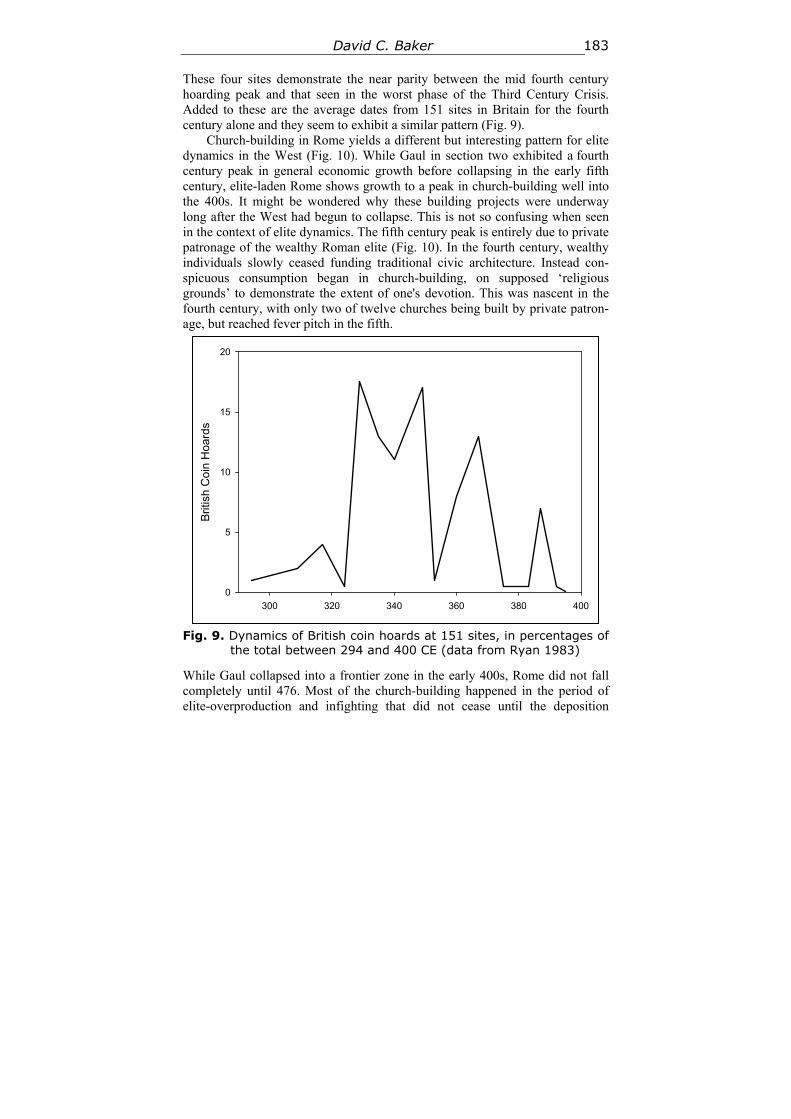
David C. Baker 183
These four sites demonstrate the near parity between the mid fourth century hoarding peak and that seen in the worst phase of the Third Century Crisis. Added to these are the average dates from 151 sites in Britain for the fourth century alone and they seem to exhibit a similar pattern (Fig. 9).
Church-building in Rome yields a different but interesting pattern for elite dynamics in the West (Fig. 10). While Gaul in section two exhibited a fourth century peak in general economic growth before collapsing in the early fifth century, elite-laden Rome shows growth to a peak in church-building well into the 400s. It might be wondered why these building projects were underway long after the West had begun to collapse. This is not so confusing when seen in the context of elite dynamics. The fifth century peak is entirely due to private patronage of the wealthy Roman elite (Fig. 10). In the fourth century, wealthy individuals slowly ceased funding traditional civic architecture. Instead con-spicuous consumption began in church-building, on supposed ‘religious grounds’ to demonstrate the extent of one's devotion. This was nascent in the fourth century, with only two of twelve churches being built by private patron-age, but reached fever pitch in the fifth.
Fig. 9. Dynamics of British coin hoards at 151 sites, in percentages of
the total between 294 and 400 CE (data from Ryan 1983)
While Gaul collapsed into a frontier zone in the early 400s, Rome did not fall completely until 476. Most of the church-building happened in the period of elite-overproduction and infighting that did not cease until the deposition
300 320 340 360 380 400
Brit
ish
Coi
n H
oard
s
0
5
10
15
20
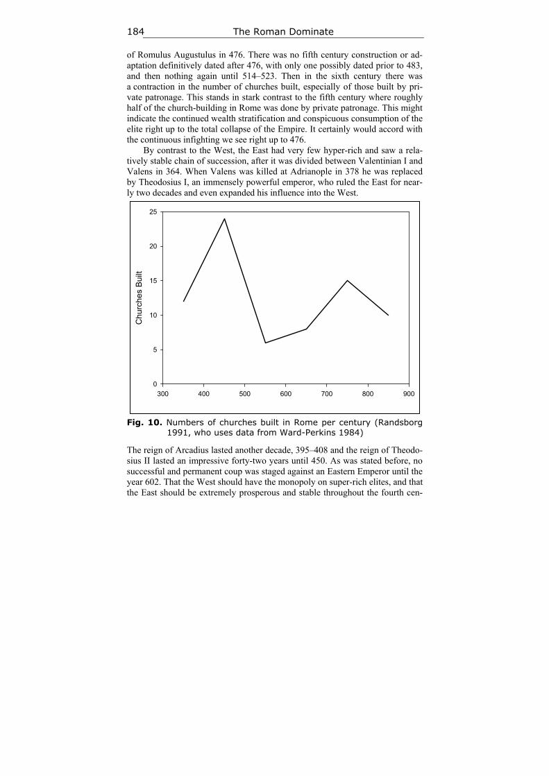
The Roman Dominate 184
of Romulus Augustulus in 476. There was no fifth century construction or ad-aptation definitively dated after 476, with only one possibly dated prior to 483, and then nothing again until 514–523. Then in the sixth century there was a contraction in the number of churches built, especially of those built by pri-vate patronage. This stands in stark contrast to the fifth century where roughly half of the church-building in Rome was done by private patronage. This might indicate the continued wealth stratification and conspicuous consumption of the elite right up to the total collapse of the Empire. It certainly would accord with the continuous infighting we see right up to 476.
By contrast to the West, the East had very few hyper-rich and saw a rela-tively stable chain of succession, after it was divided between Valentinian I and Valens in 364. When Valens was killed at Adrianople in 378 he was replaced by Theodosius I, an immensely powerful emperor, who ruled the East for near-ly two decades and even expanded his influence into the West.
Fig. 10. Numbers of churches built in Rome per century (Randsborg
1991, who uses data from Ward-Perkins 1984)
The reign of Arcadius lasted another decade, 395–408 and the reign of Theodo-sius II lasted an impressive forty-two years until 450. As was stated before, no successful and permanent coup was staged against an Eastern Emperor until the year 602. That the West should have the monopoly on super-rich elites, and that the East should be extremely prosperous and stable throughout the fourth cen-
300 400 500 600 700 800 900
Chu
rche
s B
uilt
0
5
10
15
20
25
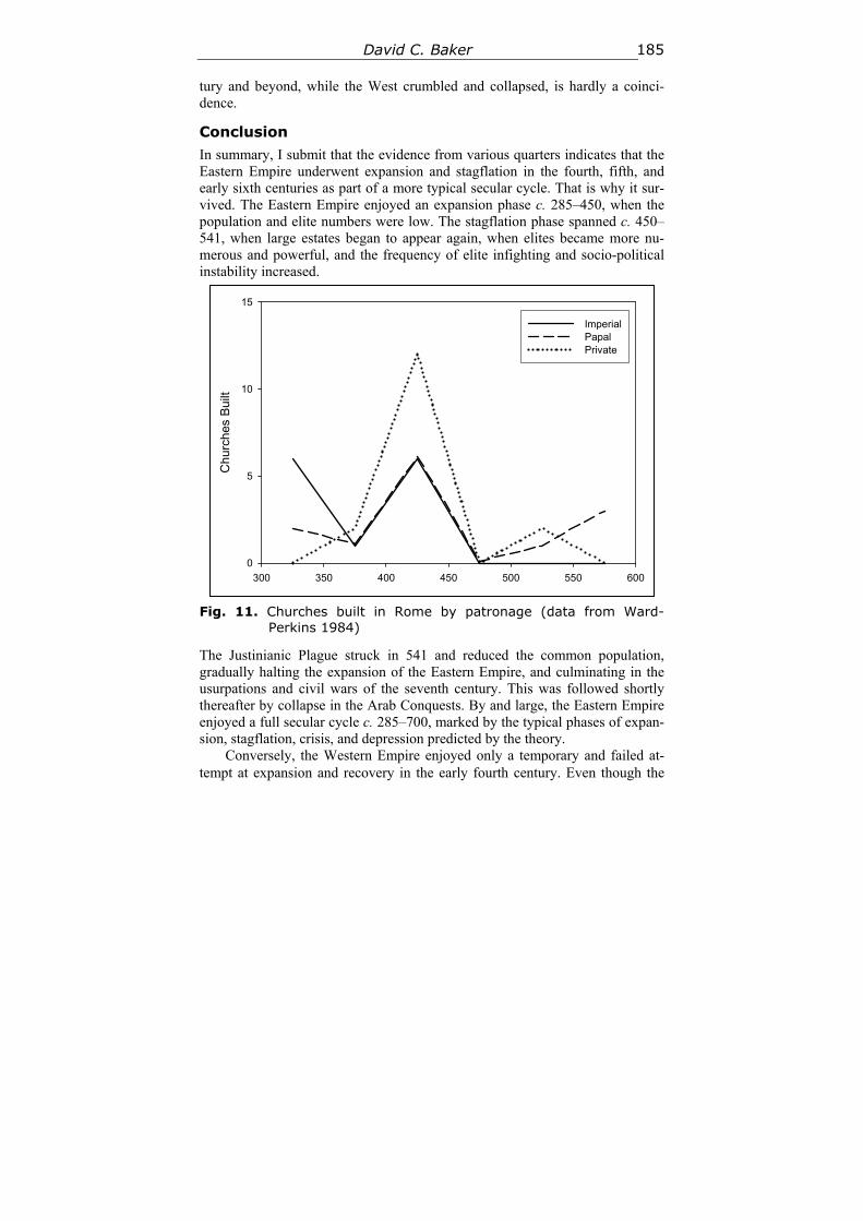
David C. Baker 185
tury and beyond, while the West crumbled and collapsed, is hardly a coinci-dence.
Conclusion
In summary, I submit that the evidence from various quarters indicates that the Eastern Empire underwent expansion and stagflation in the fourth, fifth, and early sixth centuries as part of a more typical secular cycle. That is why it sur-vived. The Eastern Empire enjoyed an expansion phase c. 285–450, when the population and elite numbers were low. The stagflation phase spanned c. 450–541, when large estates began to appear again, when elites became more nu-merous and powerful, and the frequency of elite infighting and socio-political instability increased.
Fig. 11. Churches built in Rome by patronage (data from Ward-
Perkins 1984)
The Justinianic Plague struck in 541 and reduced the common population, gradually halting the expansion of the Eastern Empire, and culminating in the usurpations and civil wars of the seventh century. This was followed shortly thereafter by collapse in the Arab Conquests. By and large, the Eastern Empire enjoyed a full secular cycle c. 285–700, marked by the typical phases of expan-sion, stagflation, crisis, and depression predicted by the theory.
Conversely, the Western Empire enjoyed only a temporary and failed at-tempt at expansion and recovery in the early fourth century. Even though the
300 350 400 450 500 550 600
Ch
urch
es B
uilt
0
5
10
15
ImperialPapalPrivate
The Roman Dominate 186
population in 285 was low enough to begin another integrative phase, and grew admirably c. 300–350, the same force that kept the West in secular depression in the Third Century Crisis still existed in the fourth century: elite dynamics. In fact the inequality ratio was on an unprecedented scale in human history. West-ern elite infighting raged continually throughout the fourth century, in stark contrast to the relative stability of the East. A recovery in the West seems likely after 285, but it probably did not last much after 350. What is more, elite in-fighting appears to have carried on throughout this period of recovery. This is significant since the most decisive variable which defines a period of secular ‘depression’ following a population crisis is the elite infighting which prevents a full demographic recovery.
Therefore, within the confines of the theory of secular cycles, the Domi-nate conforms to the predictions laid out for it. It exhibits a number of trends which perhaps explain the total collapse of the West and the survival of the East. In evaluating these trends, we explore in new ways the well-travelled evi-dence and the age-old question: what caused the decline and fall of the Roman Empire? Future studies along these lines may revolutionise the historiography of Late Antiquity and irrevocably alter the discussion of questions left unan-swered by older scholarship.
References Alcock S. 1993. Graecia Capta: The Landscapes of Roman Greece. Cambridge: Cam-
bridge University Press.
Ammianus Marcellinus 1973. Res Gestae Libri / Ed. by A. Selem. Torino: UTET.
Bagnall R. 1993. Egypt in Late Antiquity. Princeton, NY: Princeton University Press.
Bintliff J. 1994. Forest Cover, Agricultural Intensity and Population Density in Roman Imperial Boeotia, Central Greece. Evaluation of Land Surfaces Cleared from For-ests in the Mediterranean Region during the Time of the Roman Empire / Ed. by F. Burkhard et al., pp. 133–143. Stuttgart: G. Fischer Verlag.
Bintliff J. 1997. Regional Survey, Demography and the Rise of Complex Societies in the Aegean. Journal of Field Archaeology 24: 8–38.
Bowes A., and Gutteridge A. 2005. Debate: Rethinking the Later Roman Landscape. Journal of Roman Archaeology 18: 405–413.
Cauuet B. et al. 1993. Un centre sidérurgique romain de la montagne noire: le domaine des forges, Les Martys, Aude. Paris: CNRS Editions.
Chavarría A. 2004. Interpreting the Transformation of Late Roman Villas: The Case of Hispania. Landscapes of Change: Rural Evolutions in Late Antiquity and the Early Middle Ages / Ed. by N. Christie, pp. 67–102. Aldershot: Ashgate Publishing.
Chavarría A., and Lewit T. 2004. Archaeological Research on the Late Antique Coun-tryside: A Bibliographic Essay. Recent Research on the Late Antique Countryside / Ed. by W. Bowden, L. Lavan, and C. Machado, pp. 3–51. Leiden: Brill.
David C. Baker 187
Domergue C. 1990. Les Mines de la Péninsule Ibérique dans l’Antiquité Romaine. Par-is: École Française de Rome.
Duncan-Jones R. 2004. Economic Change and Transition to Late Antiquity. Approach-ing Late Antiquity: The Transformation of Early to Late Empire / Ed. by S. Swain, and M. Edwards, pp. 20–52. Oxford: Oxford University Press.
Edmondson J. C. 1989. Mining in the Later Roman Empire and Beyond: Continuity or Disruption? Journal of Roman Studies 79: 84–102.
Foss C. 1977. Archaeology and the ‘Twenty Cities’ of Byzantine Asia. American Jour-nal of Archaeology 81: 469–486.
Gatier P. 1994. Villages du Proche-Orient protobyzantin (4ème – 7ème s.) Etude région-ale. The Byzantine and Early Islamic Near East: Land Use and Settlement Patterns / Ed. by G. King, and A. Cameron, pp. 17–48. Princeton: Darwin Press.
Gerontius 1984. Life of Melania the Younger / trans. by E. Clark. Toronto: Edwin Mel-len Press.
Haldon J. 2005. Economy and Administration: How Did the Empire Work? The Cam-bridge Companion to the Age of Justinian / Ed. by M. Maas, pp. 28–59. Cambridge: Cambridge University Press.
Hong S. et al. 1994. Greenland Ice Evidence of Hemispheric Lead Pollution Two Mil-lennia Ago by Greek and Roman Civilizations. Science 5180: 1841–1843.
Hong S. et al. 1996. History of Ancient Copper Smelting Pollution During Roman and Medieval Times Recorded in Greenland Ice. Science 5259: 246–249.
Jones B., and Mattingly D. 2002. An Atlas of Roman Britain. 2nd ed. Oxford: Oxbow Books.
Koepke N., and Baten J. 2005. The Biological Standard of Living in Europe during the Last Two Millennia. European Review of Economic History 9: 61–95.
Kohler T., Cole S., and Ciupe S. 2009. Population and Warfare: A Test of the Turchin Model in Pueblo Societies. Pattern and Process in Cultural Evolution / Ed. by S. Shennan, pp. 290–291. Berkeley, CA: University of California Press.
Lee A. 1993. Information and Frontiers: Roman Foreign Relations in Late Antiquity. Cambridge: Cambridge University Press.
Lewit T. 1991. Agricultural Production in the Roman Economy AD 200–400. Oxford: Tempus Reparatum.
Lewit T. 2003. ‘Vanishing Villas’: What Happened to Elite Rural Habitation in the West in the Fifth and Sixth Centuries? Journal of Roman Archaeology 16: 260–274.
Lewit T. 2009. Pigs, Presses, and Pastoralism: Farming in the Fifth and Sixth Centuries AD. Early Medieval Europe 17: 77–91.
Loriot X., and Nony D. 1997. La crise de l'Empire romain: 235–285. Paris: Armand Colin.
Louis E. 2004. A De-Romanised Landscape in Northern Gaul: The Scarpe Valley from the Fourth to the Ninth Century AD. Late Antique Archaeology: Recent Research on the Late Antique Countryside / Ed. by W. Bowden, L. Lavan, C. Machado, pp. 479–504. Leiden: Koninklijke Brill.
The Roman Dominate 188
Mangin M. 1992. Mines et métallurgie chez les Éduens: le district sidérurgique antique et médiéval du Morvan-Auxois. Besançon: Université de Besançon.
Matthews J. 1975. Western Aristocracies and Imperial Court: AD 364–425. Oxford: Clarendon Press.
Meyer C. 1995. A Byzantine Gold-Mining Town in the Eastern Desert of Egypt: Bir Umm Fawakhir, 1992–1993. Journal of Roman Archaeology 8: 192–224.
Olympiodorus 1920. Frag. 44. In Photius. Bibliotheca. New York: Macmillan.
Ossel P. van, and Ouzoulias P. 2000. Rural Settlement Economy in Northern Gaul in the Late Empire: An Overview. Journal of Roman Archaeology 13: 133–160.
Parker A. 1992. Ancient Shipwrecks of the Mediterranean and the Roman Provinces. Oxford: Tempus Reparatum.
Pilet C. et al. 1994. La Nécropole de Saint-Martin-de-Fontenay (Calvados): Recherches sur le peuplement de la plaine de Caen du Ve s. avant J. C. au VIIe s. après J. C. Paris: CNRS Editions.
Randsborg K. 1991. The First Millennium AD in Europe and the Mediterranean: An Archaeological Essay. Cambridge: Cambridge University Press.
Ryan N. S. 1983. Fourth Century Coin Finds in Roman Britain: A Computer Analysis. Oxford: BAR British Series.
Sarris P. 2004. Rehabilitating the Great Estate: Aristocratic Property and Economic Growth in the Late Antique East. Late Antique Archaeology: Recent Research on the Late Antique Coutryside / Ed. by W. Bowden et al., pp. 55–72. Leiden: Koninklijke Brill.
Shotyk W. et al. 1998. History of Atmospheric Lead Deposition. Science 5383: 1635–1640.
Tate G. 1992. Les campagnes de la Syrie du Nord du IIe au VIIe siècle. Vol. I. Paris: Librarie orientaliste Paul Geuthner.
Turchin P. 2003. Historical Dynamics: Why States Rise and Fall. Princeton: Princeton University Press.
Turchin P. 2006. War and Peace and War: The Life Cycles of Imperial Nations. New York: Pi Press.
Turchin P., and Nefedov S. 2009. Secular Cycles. Princeton: Princeton University Press.
Ward A., Heichelheim F., and Yeo C. 1999. A History of the Roman People. 3rd ed. Upper Saddle River, NJ: Prentice-Hall.
Ward-Perkins B. 1984. From Classical Antiquity to the Middle Ages: Urban Public Building in Northern and Central Italy AD 300–850. Oxford: Oxford University Press.
Ward-Perkins B. 2005. The Fall of Rome and the End of Civilization. Oxford: Oxford University Press.
Wickham C. 2005. Framing the Early Middle Ages: Europe and the Mediterranean, 400–800. Oxford: Oxford University Press.

David C. Baker 189
Wickham C. 2009. The Inheritance of Rome: A History of Europe from 400 to 1000. London: Allen Lane.
Wightman E. 1985. Gallia Belgica. Berkeley, CA: University of California Press.
Williams S., and Friell G. 1999. The Rome that Did not Fall: The Survival of the East in the Fifth Century. London: Routledge.
Wilson A. 2009. Approaches to Quantifying Roman Trade. Quantifying the Roman Economy: Methods and Problems / Ed. by A. Bowman, and A. Wilson, pp. 219–229. Oxford: Oxford University Press.
Wood I. 1994. The Merovingian Kingdoms. London: Longman.
Zosimus 1982. New History / trans. by R. Ridley. Canberra: Australian Association for Byzantine Studies.
History & Mathematics: Trends and Cycles 2014 190–200
190
6
Modeling Malthusian Dynamics in Pre-industrial Societies:
Mathematical Modeling
Sergey A. Nefedov
Abstract
The discussion about the Malthusian character of pre-industrial economies that has arisen in the recent years extensively uses simple mathematical models. This article analyzes some of these models to determine their conformity with Malthusian postulates. The author suggests two models that are more adequate for the description of Malthusian patterns.
Keywords: Malthusianism, economic and mathematical models, population oscillations, population growth, consumption dynamics, demographic crisis, Cliodynamics.
Until recently, most economic historians have tended toward the opinion that medieval economies in Eurasia had a Malthusian nature (Allen 2008: 951). However, following the publication of Lee and Anderson's (2002) work, many came to dispute this opinion. A discussion has arisen about how the available data confirm the Malthusian relationship between demographic dynamics and consumption (i.e., real wages). This discussion has largely involved simple mathematical models of Malthusian economics.
In 1980, Lee published the first and most popular of these models. This model describes the relationship between the real wage, wt (consumption), and labor resources, Nt (population), using the following equation:
wt = exp(μ + ρt + εt) Nt–η. (Eq. 1)
Or, in logarithmic form: ln wt = μ + ρt – η ln Nt + εt. (Eq. 2)
Here, t is time; μ, ρ, η are some non-negative constants; and εt is a variable that takes into account the climatic effect and other exogenous parameters. The factor ρ describes capital increase and technological advances, thus Mal-thusian economics features ρ = 0. If we take into account that εt = 0 in the ideal case, the model can be expressed with quite a simple equation: wt = С Nt
–η, where С is some certain constant. The drawbacks of this equation are evident: a small population Nt results in a consumption rate close to infinity, while in
Sergey A. Nefedov 191
a large population the consumption becomes too small to ensure subsistence. Additionally, this equation only shows the relationship between population and consumption. The model contains no feedback to demonstrate how consump-tion influences population growth.
Wood (1998) has suggested one feedback option. Wood derives his equa-tion from the same Eq. 1 as Lee, but formulates it as follows:
wt = θ (St/Nt)η. (Eq. 1a)
Here, θ is the minimum per capita consumption rate, and St is the maxi-mum population that can subsist in the given territory when the consumption equals θ. St can grow through technological advances, but the Malthusian case features a constant St, St = S0. Wood believes that the birth rate bt and death rate dt can be described with the following equations:
bt = β0 + β1 ln wt + β2 dt , (Eq. 3) dt = δ0 + δ1 ln wt + δ2 bt , (Eq. 4)
where β0 , β1 , β2, δ0, δ1, and δ2 are certain constants. Thus, the equation below describes population growth:
dNt /dt = (bt – dt)Nt . (Eq. 5) Deriving bt and dt from the system of Eqs 3 and 4 and inserting them into
Eq. 5 yields: dNt /dt = (bt – dt)Nt = (с0 +с1 ln wt)Nt ,
where с0 and с1 are certain constants. Substituting Eq. 1a here produces: dNt /dt = (с2 + с3 ln Nt )Nt, (Eq. 6)
where с2 and с3 are certain constants. The differential Eq. 6 has the time-independent solution Nt = N0 = exp(–с2/с3); its chart will be a horizontal line. According to the theorem of the unique existence of the solution, no other solu-tions (integral curves) may cross this horizontal line. The derivative dNt /dt is positive below this line, in the area 0 < Nt < N0; the solutions monotonically increase and the integral curves approximate the horizontal line. The derivative dNt /dt is negative above this line; the solutions monotonically decrease and the integral curves approximate the horizontal line from above. Finally, the solu-tions cannot oscillate: the population cannot first feature growth and then loss due to ‘Malthusian crisis’. Wood justifies this behavior of his model stating that Malthusian crises ‘are not a necessary feature of Malthusian systems… This conclusion is contrary to the belief of many economic historians (e.g., Le Roy Ladurie 1974: passim; Postan and Hatcher 1985: 69) though not to anything that Malthus himself ever wrote’ (Wood 1998: 110).
Malthus did, however, write about population loss, depopulation:
The power of population is so superior to the power of the earth to produce subsistence for man, that premature death must in some shape or other visit the human race. The vices of mankind are active and able ministers of depopulation. They are the precursors in the great army of destruction, and often finish the dreadful work them-
Malthusian Dynamics in Pre-industrial Societies 192
selves. But should they fail in this war of extermination, sickly sea-sons, epidemics, pestilence, and plague advance in terrific array, and sweep off their thousands and tens of thousands. Should success be still incomplete, gigantic inevitable famine stalks in the rear, and with one mighty blow levels the population with the food of the world (Malthus 1798: 61).
Wood's model does not, therefore, describe the population dynamics envi-sioned by Malthus himself. It is nonetheless used in many studies dedicated to the analysis of the Malthusian economics in traditional societies.
Sometimes an iterative version of this model is used, implying calculations on an annual basis. Eq. 1a in the version put forth by Møller and Sharp (2009) has logarithmic form:
ln wt = c0 – c1 ln Nt + ln A. (Eq. 2a) Birth and death rates are calculated from the simplified equations:
bt = a0 + a1 ln wt , (Eq. 3a) dt = a2 – a3 ln wt . (Eq. 4a)
The population Nt is related to the population Nt–1 in the previous year through the following relationship:
ln Nt = ln Nt–1 +bt–1 – dt–1. (Eq. 7) Here, A, c0, c1, a0 … a3 are certain constants. Inserting Eqs 3a and 4a into Eq. 7 gives:
ln Nt = ln Nt–1 + (a1 + a3) ln Wt–1 + a0 – a2= = ln Nt–1 + (a1 + a3)(c0 – c1 ln Nt–1 + ln A) + a0 – a2 = u ln Nt–1 + ln v,
where u and v are certain constants. The resulting equation is: Nt = v(Nt–1)
u. (Eq. 8) This equation generates a series of population values. If the population at
the initial moment equals 1 million (i.e., N1 = 1), then N2 = v, N3 equals v raised to a power of 1 + u , N3 equals to v raised to a power of 1 + u + u2, etc. If ׀u1 < ׀, then Nt → ∞, which is impossible under the condition of limited resources in the Malthusian theory. If 0 < u < 1, then Nt monotonically tends to a finite bound. Finally, the case –1 < u < 0 produces a very specific series in which the population increases in even years and decreases in odd years (or vice versa). Thus, the Møller-Sharp model has the same drawback as Wood's initial model: it cannot describe long-term population oscillations.
Another iterative version of the model is that developed by Ashraf and Ga-lor (2011). Beginning with Eq. 1a, the authors of this model take into consid-eration the number of adults and children, and optimize expenses. They, never-theless, ultimately come to the same Eq. 8.
One more version of Wood's model is that of Voigtlander and Voth (2009). They use Eq. 1a, but replace Eqs 3 and 4 with Eqs 3a and 4a:
bt = b0 (wt / θ)m, (Eq. 3a) dt =d0 (wt / θ)n, (Eq. 4a)
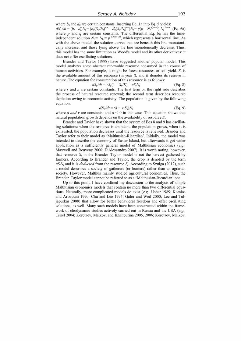
Sergey A. Nefedov 193
where b0 and d0 are certain constants. Inserting Eq. 1a into Eq. 5 yields: dNt /dt = (bt – dt)Nt = (b0(S0/Nt)
ηm – d0(S0/Nt)ηn)Nt = q(p – Nt
η(m–n)) Nt 1–ηm, (Eq. 6a)
where p and q are certain constants. The differential Eq. 6a has the time-independent solution Nt = N0 = p
1/η(m–n), which represents a horizontal line. As with the above model, the solution curves that are beneath this line monotoni-cally increase, and those lying above the line monotonically decrease. Thus, this model has the same limitation as Wood's model and its other derivatives: it does not offer oscillating solutions.
Brander and Taylor (1998) have suggested another popular model. This model analyzes some abstract renewable resource consumed in the course of human activities. For example, it might be forest resources or soil yield. St is the available amount of this resource (in year t), and K denotes its reserve in nature. The equation for consumption of this resource is as follows:
dSt /dt = rSt (1 – St /K) – uStNt, (Eq. 8) where r and u are certain constants. The first term on the right side describes the process of natural resource renewal; the second term describes resource depletion owing to economic activity. The population is given by the following equation:
dNt /dt = (d + v S t)Nt, (Eq. 9) where d and v are constants, and d < 0 in this case. This equation shows that natural population growth depends on the availability of resource St.
Brander and Taylor have shown that the system of Eqs 8 and 9 has oscillat-ing solutions: when the resource is abundant, the population grows, when it is exhausted, the population decreases until the resource is renewed. Brander and Taylor refer to their model as ‘Malthusian-Ricardian’. Initially, the model was intended to describe the economy of Easter Island, but afterwards it got wider application as a sufficiently general model of Malthusian economics (e.g., Maxwell and Reuveny 2000; D'Alessandro 2007). It is worth noting, however, that resource St in the Brander–Taylor model is not the harvest gathered by farmers. According to Brander and Taylor, the crop is denoted by the term uStNt and it is deducted from the resource St. According to Szulga (2012), such a model describes a society of gatherers (or hunters) rather than an agrarian society. However, Malthus mainly studied agricultural economies. Thus, the Brander–Taylor model cannot be referred to as a ‘Malthusian-Ricardian’ one.
Up to this point, I have confined my discussion to the analysis of simple Malthusian economics models that contain no more than two differential equa-tions. Naturally, more complicated models do exist (e.g., Usher 1989; Komlos and Artzrouni 1990; Chu and Lee 1994; Galor and Weil 2000; Lee and Tul-japurkar 2008) that allow for better behavioral freedom and offer oscillating solutions, as well. Many such models have been constructed within the frame-work of cliodynamic studies actively carried out in Russia and the USA (e.g., Tsirel 2004; Korotaev, Malkov, and Khaltourina 2005, 2006; Korotaev, Malkov,
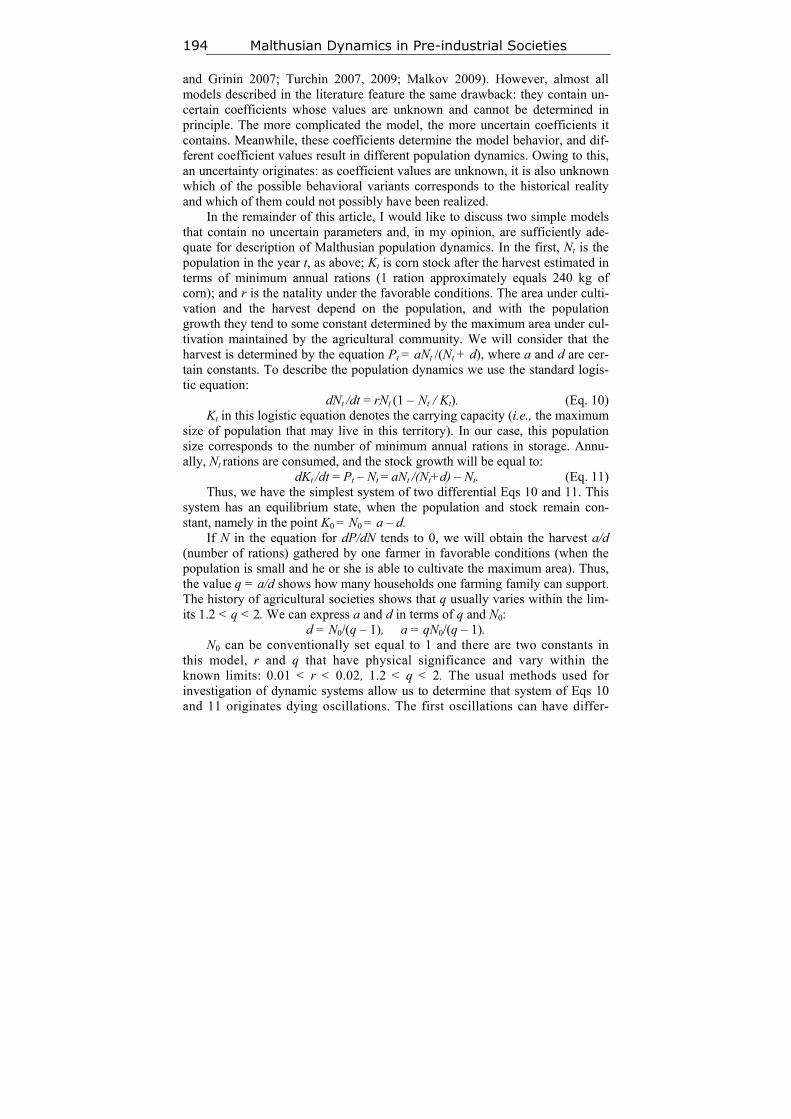
Malthusian Dynamics in Pre-industrial Societies 194
and Grinin 2007; Turchin 2007, 2009; Malkov 2009). However, almost all models described in the literature feature the same drawback: they contain un-certain coefficients whose values are unknown and cannot be determined in principle. The more complicated the model, the more uncertain coefficients it contains. Meanwhile, these coefficients determine the model behavior, and dif-ferent coefficient values result in different population dynamics. Owing to this, an uncertainty originates: as coefficient values are unknown, it is also unknown which of the possible behavioral variants corresponds to the historical reality and which of them could not possibly have been realized.
In the remainder of this article, I would like to discuss two simple models that contain no uncertain parameters and, in my opinion, are sufficiently ade-quate for description of Malthusian population dynamics. In the first, Nt is the population in the year t, as above; Kt is corn stock after the harvest estimated in terms of minimum annual rations (1 ration approximately equals 240 kg of corn); and r is the natality under the favorable conditions. The area under culti-vation and the harvest depend on the population, and with the population growth they tend to some constant determined by the maximum area under cul-tivation maintained by the agricultural community. We will consider that the harvest is determined by the equation Pt = aNt /(Nt + d), where a and d are cer-tain constants. To describe the population dynamics we use the standard logis-tic equation:
dNt /dt = rNt (1 – Nt / Kt). (Eq. 10) Kt in this logistic equation denotes the carrying capacity (i.e., the maximum
size of population that may live in this territory). In our case, this population size corresponds to the number of minimum annual rations in storage. Annu-ally, Nt rations are consumed, and the stock growth will be equal to:
dKt /dt = Pt – Nt = aNt /(Nt+d) – Nt. (Eq. 11) Thus, we have the simplest system of two differential Eqs 10 and 11. This
system has an equilibrium state, when the population and stock remain con-stant, namely in the point K0 = N0 = a – d.
If N in the equation for dP/dN tends to 0, we will obtain the harvest a/d (number of rations) gathered by one farmer in favorable conditions (when the population is small and he or she is able to cultivate the maximum area). Thus, the value q = a/d shows how many households one farming family can support. The history of agricultural societies shows that q usually varies within the lim-its 1.2 < q < 2. We can express a and d in terms of q and N0:
d = N0/(q – 1), a = qN0/(q – 1). N0 can be conventionally set equal to 1 and there are two constants in
this model, r and q that have physical significance and vary within the known limits: 0.01 < r < 0.02, 1.2 < q < 2. The usual methods used for investigation of dynamic systems allow us to determine that system of Eqs 10 and 11 originates dying oscillations. The first oscillations can have differ-
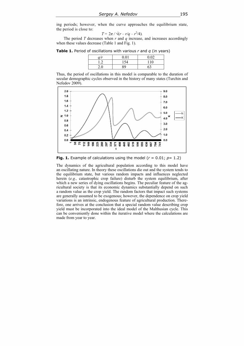
Sergey A. Nefedov 195
ing periods; however, when the curve approaches the equilibrium state, the period is close to:
T = 2π / √(r – r/q – r2/4). The period T decreases when r and q increase, and increases accordingly
when these values decrease (Table 1 and Fig. 1).
Table 1. Period of oscillations with various r and q (in years)
q/r 0.01 0.02 1.2 154 110 2.0 89 63
Thus, the period of oscillations in this model is comparable to the duration of secular demographic cycles observed in the history of many states (Turchin and Nefedov 2009).
Fig. 1. Example of calculations using the model (r = 0.01; p= 1.2)
The dynamics of the agricultural population according to this model have an oscillating nature. In theory these oscillations die out and the system tends to the equilibrium state, but various random impacts and influences neglected herein (e.g., catastrophic crop failure) disturb the system equilibrium, after which a new series of dying oscillations begins. The peculiar feature of the ag-ricultural society is that its economic dynamics substantially depend on such a random value as the crop yield. The random factors that impact such systems are generally assumed to be exogenous; however, the dependence on crop yield variations is an intrinsic, endogenous feature of agricultural production. There-fore, one arrives at the conclusion that a special random value describing crop yield must be incorporated into the ideal model of the Malthusian cycle. This can be conveniently done within the iterative model where the calculations are made from year to year.
Malthusian Dynamics in Pre-industrial Societies 196
For convenience, I consider production years that start with the harvest, not a specific calendar date. The population size Nt at the beginning of year t is expressed in terms of the number of households or families (conventionally assuming that a household population is 5 people). In theory (i.e., when there is enough land for cultivation), a farming household cultivates a standard parcel of land (e.g., a Middle Eastern ‘çiftlik’) and one can measure the maximum possible area of arable land in terms of standard parcels S. When the number of households Nt exceeds S, two families can live on some parcels.
Let at represent the annual crop yield t, expressed in terms of minimum family corn rations that can be gathered on a standard parcel. We will express the crop yield in the form at = a0 + dt, where a0 is the average crop yield, dt is a random value that accepts values from the segment (–а1, а1). The value а1 is less than a0 and the crop yield at varies within the interval of a0 – а1 to a0 + а1. With the units of measure that I have assumed, the harvest Yt (number of ra-tions) can be expressed in the following simple form:
Yt = atNt if Nt < S, and Yt = atS if Nt > S. If there is corn surplus in the year t, that is per-capita production yt = Yt/Nt
exceeds some value of ‘satisfactory consumption’ p1 (p1 > 1), then the farmers do not consume the entire corn produced, but lay up some surplus portion in store (for simplicity sake we will assume that they lay up half the surplus). However, it is worth noting that, owing to the storage conditions, the household stock Zt cannot grow to infinity and is limited by certain value Z0. If there are surpluses exceeding this value, they all are consumed. If the year is lean and the production yt falls below the level p1, the farmers take corn from the stock, in-creasing the consumption, if possible, up to the level p1. If the stock is not suf-ficient, it is consumed in full.
The population growth rate rt is determined as the ratio of the population Nt+1 in the following year to the population Nt in the previous year. The growth rate rt depends on the consumption pt. When the consumption is equal to the minimum normal rate (pt = 1), the population remains constant (rt = 1). I desig-nate the maximum natural growth r0, and the consumption rate needed to en-sure it – p0. I believe that r0 = 1.02, that the maximum population growth is 2 % yearly. When 1 < pt < p0, population growth is linearly dependent on con-sumption, and in the case when pt > p0, it does not increase (r = r0). For pt < 1, the dependence of rt on pt is taken as rt = pt (i.e., in case of crop failure the sur-viving population will be equal to the number of rations and all people that do not have a sufficient annual food reserve will perish from starvation). Conse-quently, the population in the following year will be Nt + 1 = rt Nt.
Considering the typical case from the Middle East or Russia in the six-teenth to eighteenth centuries, in which each family could obtain two minimal rations from one standard parcel, one can assume a0 = 2 for the numerical ex-periment. The scatter of crop yield (ratio а1 /a0) was large enough (e.g., it was about 60 % of average crop yield in Egypt). Hence, it appears that one can as-
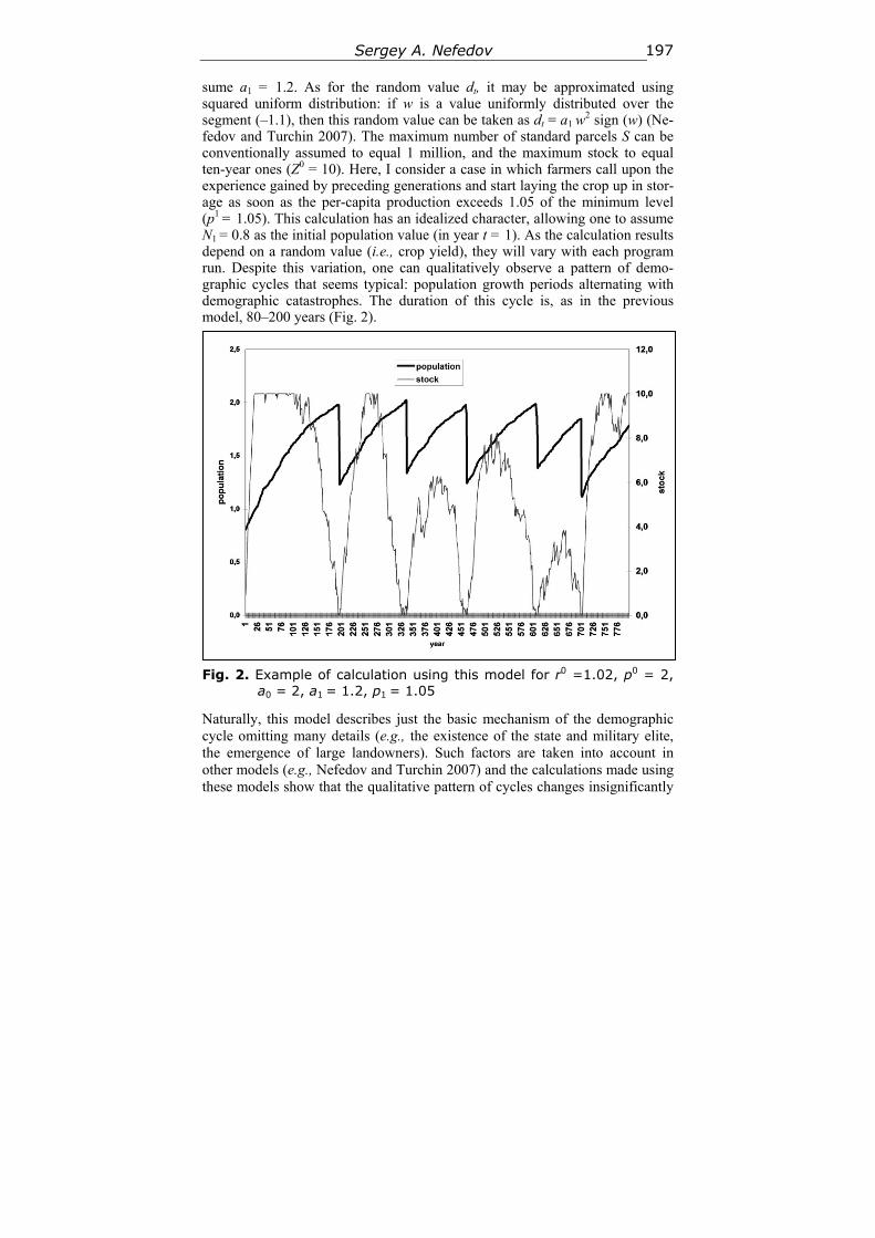
Sergey A. Nefedov 197
sume а1 = 1.2. As for the random value dt, it may be approximated using squared uniform distribution: if w is a value uniformly distributed over the segment (–1.1), then this random value can be taken as dt = а1 w
2 sign (w) (Ne-fedov and Turchin 2007). The maximum number of standard parcels S can be conventionally assumed to equal 1 million, and the maximum stock to equal ten-year ones (Z0 = 10). Here, I consider a case in which farmers call upon the experience gained by preceding generations and start laying the crop up in stor-age as soon as the per-capita production exceeds 1.05 of the minimum level (p1 = 1.05). This calculation has an idealized character, allowing one to assume N1 = 0.8 as the initial population value (in year t = 1). As the calculation results depend on a random value (i.e., crop yield), they will vary with each program run. Despite this variation, one can qualitatively observe a pattern of demo-graphic cycles that seems typical: population growth periods alternating with demographic catastrophes. The duration of this cycle is, as in the previous model, 80–200 years (Fig. 2).
Fig. 2. Example of calculation using this model for r0 =1.02, p0 = 2,
a0 = 2, а1 = 1.2, p1 = 1.05
Naturally, this model describes just the basic mechanism of the demographic cycle omitting many details (e.g., the existence of the state and military elite, the emergence of large landowners). Such factors are taken into account in other models (e.g., Nefedov and Turchin 2007) and the calculations made using these models show that the qualitative pattern of cycles changes insignificantly
Malthusian Dynamics in Pre-industrial Societies 198
compared to the suggested model. On the whole, it seems quite certain that the availability of corn stock in farms allows for long-term economic stabilization. Population growth results in stock depletion, however, and, sooner or later, major harvest failures provoke catastrophic starvations followed by events like epidemics, uprisings of starving people, and/or invasions by external enemies seeking to take advantage. As a result, the population size can decrease even by half and a new demographic cycle starts. While the model calculations suggest that this new cycle might start immediately after the catastrophe, in real life such crises as wars and uprisings have some inertia and impede economic re-vival. In such cases, stabilization is delayed.
Finally, it is worth noting that after the publication of Wood's model eco-nomic historians came to see Malthusian economics as a system wherein the population size cannot exceed the carrying capacity and, consequently, the ‘Malthusian crisis’ is not possible. For example, Read and LeBlanc (2003: 59) ‘… suggest that there is a standard model for the pattern of human population growth and its relationship to carrying capacity (K), namely, that most of the time human populations have low to nonexistent rates of growth… The model is often implicit and may simply assert that, until recently, population sizes have always been well below K and growth rates very low’. But Le Roy La-durie, Postan, Hatcher and many other economic historians insist that ‘Mal-thusian crises’ were quite common phenomena in lived history, a fact ac-knowledged by Wood himself. The models described in this article show that the inevitability of similar crises arises from the simple laws that govern the functioning of agrarian economies.
References
Allen R. 2008. A Review of Gregory Clark's a Farewell to Alms: A Brief Economic History of the World. Journal of Economic Literature 46: 946–973.
Ashraf Q., and Galor O. 2011. Dynamics and Stagnation in the Malthusian Epoch. American Economic Review 101(5): 2003–2041.
Brander J., and Taylor M. 1998. The Simple Economics of Easter Island: A Ricardo-Malthus Model of Renewable Resource Use. The American Economic Review 88: 119–138.
Chu C. Y. C., and Lee R. D. 1994. Famine, Revolt, and the Dynastic Cycle. Journal of Population Economics 7(4): 351–378.
D'Alessandro S. 2007. Non-Linear Dynamics of Population and Natural Resources: The Emergence of Different Patterns of Development. Ecological Economics 62: 473–481.
Galor O., and Weil D. N. 2000. Population, Technology, and Growth: From Malthu-sian Stagnation to the Demographic Transition and Beyond. The American Eco-nomic Review 90(4): 806–828.
Sergey A. Nefedov 199
Komlos J., and Artzrouni M. 1990. Mathematical Investigations of the Escape from the Malthusian Trap. Mathematical Population Studies 2: 269–287.
Korotaev A., Malkov S., and Grinin L. (Eds.) 2007. History and Mathematics: Analysis and Modeling of Socio-Historical Processes. Moscow: URSS. In Russian (Коротаев А., Малков С., Гринин Л. (ред.) История и Математика: Анализ и моделирование социально-исторических процессов. М.: УРСС).
Korotaev A., Malkov A., and Khaltourina D. 2005. Laws of History. Mathematical Modeling of Historical Macro-Processes: Demography, the Economy, Wars. Mos-cow: URSS. In Russian (Коротаев А. В., Малков А. С., Халтурина Д. А. Законы истории. Математическое моделирование исторических макропроцессов. Де-мография, экономика, войны. М.: УРСС).
Korotaev A., Malkov A., and Khaltourina D. 2006. Introduction to Social Macrody-namics: Secular Cycles and Millennial Trends. Moscow: Komkniga.
Le Roy Ladurie E. 1974. The Peasants of Languedoc. Urbana, IL: University of Illinois Press.
Lee R. 1980. A Historical Perspective on Economic Aspects of the Population Explo-sion: The Case of Preindustrial England. Population and Economic Change in De-veloping Countries / Ed. by R. A. Easterlin, pp. 517–566. Chicago, IL: University of Chicago Press.
Lee R., and Anderson M. 2002. Malthus in State Space: Macro Economic–Demographic Relations in English History, 1540–1870. Journal of Population Eco-nomics 15(2): 195–220.
Lee C. T., and Tuljapurkar S. 2008. Population and Prehistory I: Food-Dependent Population Growth in Constant Environments. Theoretical Population Biology 73: 473–482.
Malkov S. 2009. Social Self-Organization and the Historical Process: The Possibilities of Mathematical Modeling. Moscow: URSS. In Russian (Малков С. Ю. Социаль-ная самоорганизация и исторический процесс: Возможности математиче-ского моделирования. М.: УРСС).
Malthus T. R. 1798. An Essay on the Principle of Population. London: J. Johnson.
Maxwell J., and Reuveny R. 2000. Resource Scarcity and Conflict in Developing Countries. Journal of Peace Research 37(3): 301–322.
Møller N., and Sharp P. 2009. Malthus in Cointegration Space: A New Look at Living Standards and Population in Pre-Industrial England. Discussion Paper No. 08–16. Copenhagen: Department of Economics, University of Copenhagen.
Nefedov S. A., and Turchin P. 2007. Experience of Modeling Demographic and Struc-tural Cycles. History and Mathematics: Macro-Historical Dynamics of Society and the State / Ed. by S. Malkov, L. Grinin, and A. Korotaev, рр. 153–167. Moscow: URSS. In Russian (Нефедов С. А., Турчин П. В. Опыт моделирования демо-графически-структурных циклов. История и математика: Макроисториче-ская динамика общества и государства / Ред. С. Ю. Малков, Л. Е. Гринин, А. В. Коротаев, c. 153–167. М.: УРСС).
Malthusian Dynamics in Pre-industrial Societies 200
Postan M. M., and Hatcher J. 1985. Population and Class Relations in Feudal Society. The Brenner Debate: Agrarian Class Structure and Economic Development in Pre-Industrial Europe / Ed. by T. Aston, and C. H. E. Philpin, pp. 65–78. Cambridge: Cambridge University Press.
Read D. W., and LeBlanc S. A. 2003. Population Growth, Carrying Capacity, and Conflict. Current Anthropology 44(1): 59–85.
Szulga R. S. 2012. Endogenous Population and Resource Cycles in Historical Hunter-Gatherer Economies. Cliodynamics 3(2): 234–270.
Tsirel S. V. 2004. On the Possible Reasons for the Hyperexponential Growth of the Earth Population. Mathematical Modeling of Social and Economic Dynamics / Ed. by M. Dmitriev, and A. Petrov, pр. 367–369. Moscow: Russian State Social Univer-sity.
Turchin P. 2007. Historical Dynamics: Towards a Theoretical History. Moscow: LKI. In Russian (Турчин Р. Историческая динамика. На пути к теоретической ис-тории. М.: ЛКИ).
Turchin P. 2009. Long-Term Population Cycles in Human Societies. Annals of the New York Academy of Science 1162: 1–17.
Turchin P., and Nefedov S. A. 2009. Secular Cycles. Princeton, NY: Princeton Univer-sity Press.
Usher D. 1989. The Dynastic Cycle and the Stationary State. The American Economic Review 79(5): 1031–1044.
Voigtlander N., and Voth H. J. 2009. Malthusian Dynamism and the Rise of Europe: Make War, Not Love. American Economic Review: Papers & Proceedings 99(2): 248–254.
Wood J. W. 1998. A Theory of Preindustrial Population Dynamics, Demography, Economy, and Well-Being in Malthusian Systems. Current Anthropology 39: 99–135.
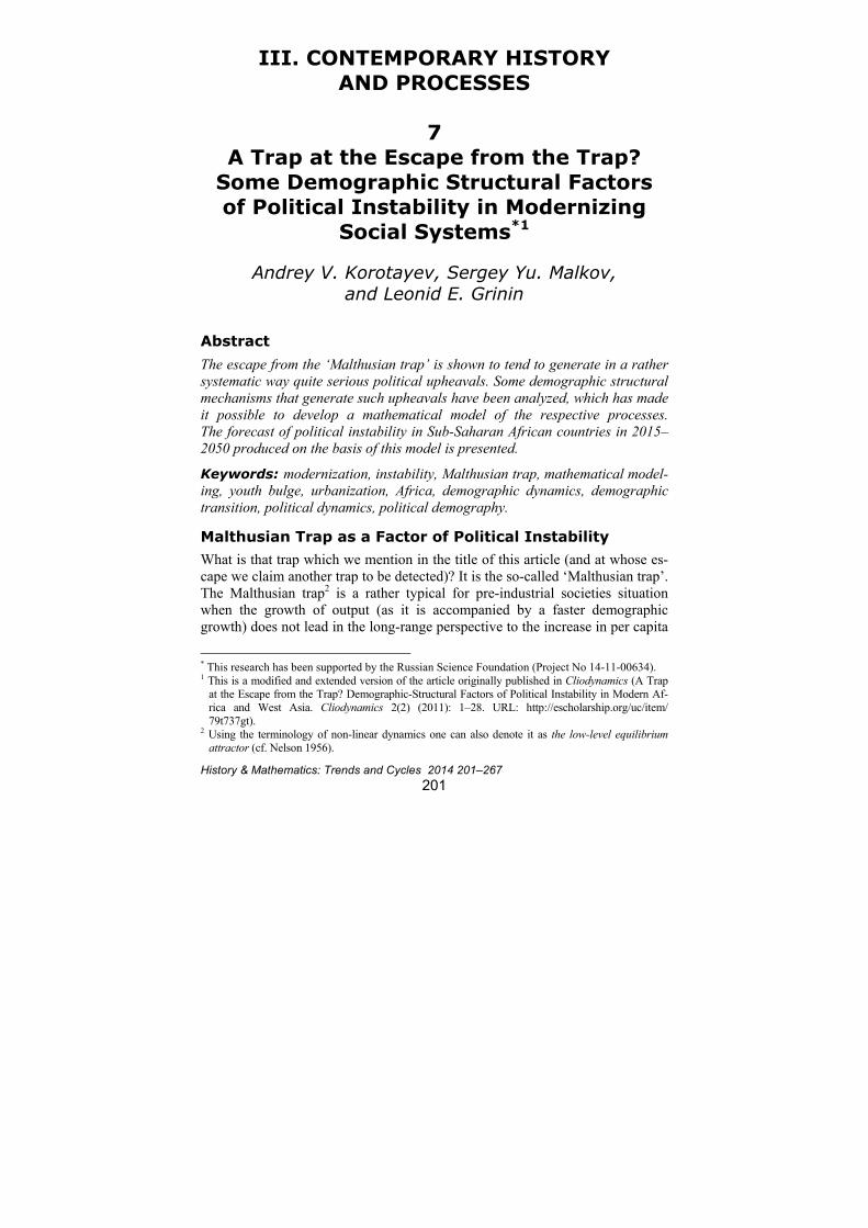
History & Mathematics: Trends and Cycles 2014 201–267
201
III. CONTEMPORARY HISTORY AND PROCESSES
7
A Trap at the Escape from the Trap? Some Demographic Structural Factors of Political Instability in Modernizing
Social Systems*1
Andrey V. Korotayev, Sergey Yu. Malkov,
and Leonid E. Grinin
Abstract
The escape from the ‘Malthusian trap’ is shown to tend to generate in a rather systematic way quite serious political upheavals. Some demographic structural mechanisms that generate such upheavals have been analyzed, which has made it possible to develop a mathematical model of the respective processes. The forecast of political instability in Sub-Saharan African countries in 2015–2050 produced on the basis of this model is presented.
Keywords: modernization, instability, Malthusian trap, mathematical model-ing, youth bulge, urbanization, Africa, demographic dynamics, demographic transition, political dynamics, political demography.
Malthusian Trap as a Factor of Political Instability
What is that trap which we mention in the title of this article (and at whose es-cape we claim another trap to be detected)? It is the so-called ‘Malthusian trap’. The Malthusian trap2 is a rather typical for pre-industrial societies situation when the growth of output (as it is accompanied by a faster demographic growth) does not lead in the long-range perspective to the increase in per capita
* This research has been supported by the Russian Science Foundation (Project No 14-11-00634). 1 This is a modified and extended version of the article originally published in Cliodynamics (A Trap
at the Escape from the Trap? Demographic-Structural Factors of Political Instability in Modern Af-rica and West Asia. Cliodynamics 2(2) (2011): 1–28. URL: http://escholarship.org/uc/item/ 79t737gt).
2 Using the terminology of non-linear dynamics one can also denote it as the low-level equilibrium attractor (cf. Nelson 1956).
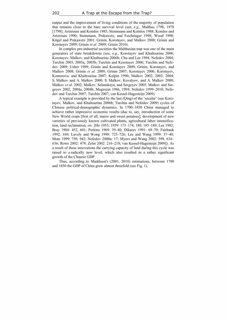
A Trap at the Escape from the Trap? 202
output and the improvement of living conditions of the majority of population that remains close to the bare survival level (see, e.g., Malthus 1798, 1978 [1798]; Artzrouni and Komlos 1985; Steinmann and Komlos 1988; Komlos and Artzrouni 1990; Steinmann, Prskawetz, and Feichtinger 1998; Wood 1998; Kögel and Prskawetz 2001; Grinin, Korotayev, and Malkov 2008; Grinin and Korotayev 2009; Grinin et al. 2009; Grinin 2010).
In complex pre-industrial societies the Malthusian trap was one of the main generators of state breakdowns (see, e.g., Korotayev and Khaltourina 2006; Korotayev, Malkov, and Khaltourina 2006b; Chu and Lee 1994; Nefedov 2004; Turchin 2003, 2005a, 2005b; Turchin and Korotayev 2006; Turchin and Nefe-dov 2009; Usher 1989; Grinin and Korotayev 2009; Grinin, Korotayev, and Malkov 2008; Grinin et al. 2009; Grinin 2007; Korotayev 2006; Korotayev, Komorova, and Khaltourina 2007; Kulpin 1990; Malkov 2002, 2003, 2004; S. Malkov and А. Malkov 2000; S. Malkov, Kovalyov, and А. Malkov 2000; Malkov et al. 2002; Malkov, Selunskaya, and Sergeyev 2005; Malkov and Ser-geyev 2002, 2004а, 2004b; Mugruzin 1986, 1994; Nefedov 1999–2010; Nefe-dov and Turchin 2007; Turchin 2007; van Kessel-Hagesteijn 2009).
A typical example is provided by the last (Qing) of the ‘secular’ (see Koro-tayev, Malkov, and Khaltourina 2006b; Turchin and Nefedov 2009) cycles of Chinese political-demographic dynamics. In 1700–1850 China managed to achieve rather impressive economic results (due to, say, introduction of some New World crops [first of all, maize and sweet potatoes], development of new varieties of previously known cultivated plants, agricultural labor intensifica-tion, land reclamation, etc. [Ho 1955; 1959: 173–174, 180, 185–189; Lee 1982; Bray 1984: 452, 601; Perkins 1969: 39–40; Dikarev 1991: 69–70; Fairbank 1992: 169; Lavely and Wong 1998: 725–726; Lee and Wang 1999: 37–40; Mote 1999: 750, 942; Nefedov 2000a: 17; Myers and Wang 2002: 599, 634–636; Rowe 2002: 479; Zelin 2002: 216–218; van Kessel-Hagesteijn 2009]). As a result of these innovations the carrying capacity of land during this cycle was raised to a radically new level, which also resulted in a rather significant growth of the Chinese GDP.
Thus, according to Maddison's (2001, 2010) estimations, between 1700 and 1850 the GDP of China grew almost threefold (see Fig. 1).
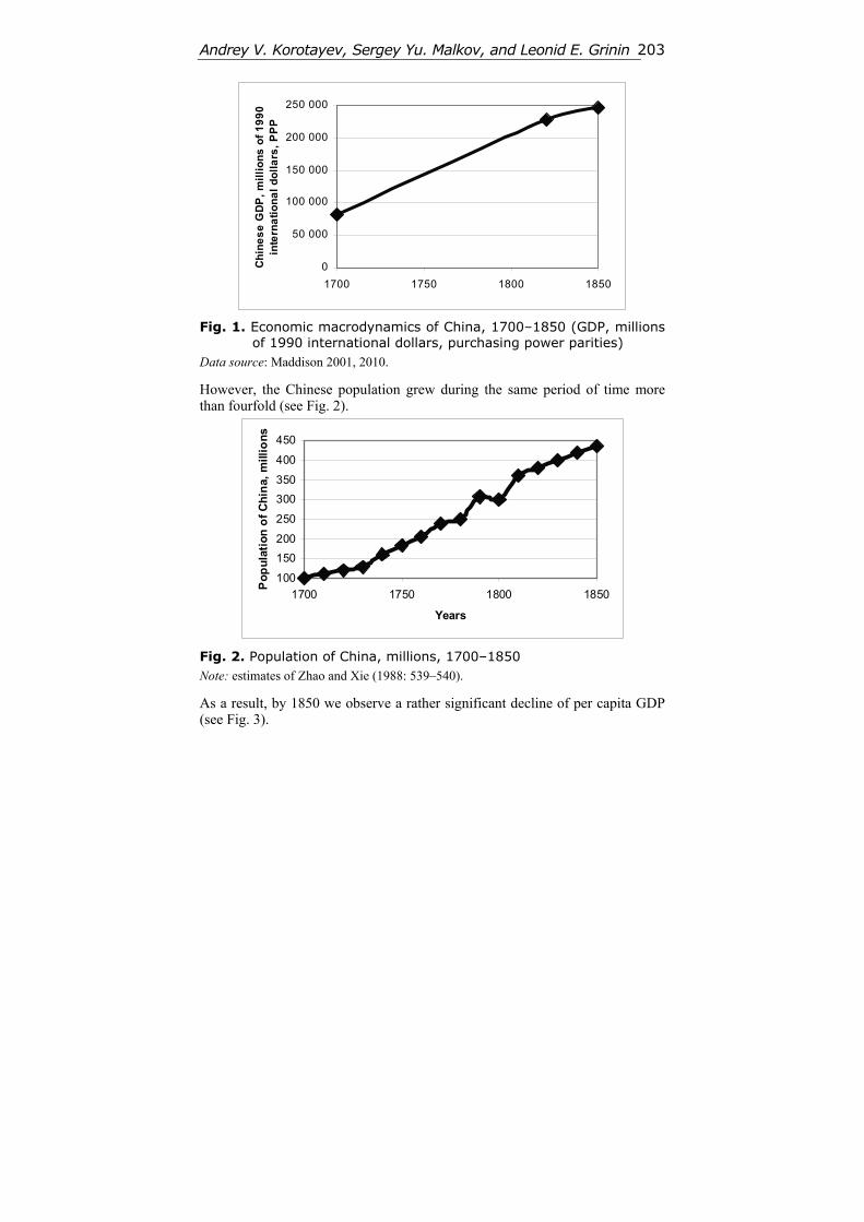
Andrey V. Korotayev, Sergey Yu. Malkov, and Leonid E. Grinin 203
0
50 000
100 000
150 000
200 000
250 000
1700 1750 1800 1850
Ch
ine
se
GD
P,
mil
lio
ns
of
19
90
in
tern
ati
on
al
do
lla
rs,
PP
P
Fig. 1. Economic macrodynamics of China, 1700–1850 (GDP, millions
of 1990 international dollars, purchasing power parities) Data source: Maddison 2001, 2010.
However, the Chinese population grew during the same period of time more than fourfold (see Fig. 2).
100
150
200
250
300
350
400
450
1700 1750 1800 1850
Years
Po
pu
lati
on
of
Ch
ina,
mill
ion
s
Fig. 2. Population of China, millions, 1700–1850 Note: estimates of Zhao and Xie (1988: 539–540).
As a result, by 1850 we observe a rather significant decline of per capita GDP (see Fig. 3).
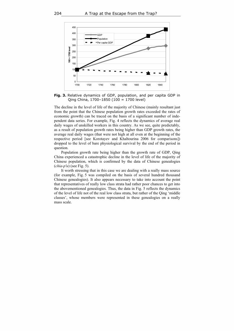
A Trap at the Escape from the Trap? 204
0
50
100
150
200
250
300
350
400
450
1700 1720 1740 1760 1780 1800 1820 1840
100
= 1
700
leve
l
GDP
Population
Per capita GDP
Fig. 3. Relative dynamics of GDP, population, and per capita GDP in
Qing China, 1700–1850 (100 = 1700 level)
The decline in the level of life of the majority of Chinese (mainly resultant just from the point that the Chinese population growth rates exceeded the rates of economic growth) can be traced on the basis of a significant number of inde-pendent data series. For example, Fig. 4 reflects the dynamics of average real daily wages of unskilled workers in this country. As we see, quite predictably, as a result of population growth rates being higher than GDP growth rates, the average real daily wages (that were not high at all even at the beginning of the respective period [see Korotayev and Khaltourina 2006 for comparisons]) dropped to the level of bare physiological survival by the end of the period in question.
Population growth rate being higher than the growth rate of GDP, Qing China experienced a catastrophic decline in the level of life of the majority of Chinese population, which is confirmed by the data of Chinese genealogies (chia-p'u) (see Fig. 5).
It worth stressing that in this case we are dealing with a really mass source (for example, Fig. 5 was compiled on the basis of several hundred thousand Chinese genealogies). It also appears necessary to take into account the point that representatives of really low class strata had rather poor chances to get into the abovementioned genealogies. Thus, the data in Fig. 5 reflects the dynamics of the level of life not of the real low class strata, but rather of the Qing ‘middle classes’, whose members were represented in these genealogies on a really mass scale.
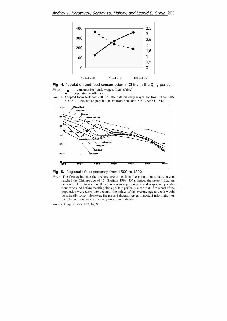
Andrey V. Korotayev, Sergey Yu. Malkov, and Leonid E. Grinin 205
0
100
200
300
400
0
0,5
1
1,5
2
2,5
3
3,5
1730–1750 1750–1800 1800–1820
Fig. 4. Population and food consumption in China in the Qing period Note: - - - ▄ - - – consumption (daily wages, liters of rice);
––♦–– – population (millions). Source: Adopted from Nefedov 2003: 5. The data on daily wages are from Chao 1986:
218–219. The data on population are from Zhao and Xie 1988: 541–542.
Fig. 5. Regional life expectancy from 1500 to 1800 Note: ‘The figures indicate the average age at death of the population already having
reached the Chinese age of 15’ (Heijdra 1998: 437); hence, the present diagram does not take into account those numerous representatives of respective popula-tions who died before reaching this age. It is perfectly clear that, if this part of the population were taken into account, the values of the average age at death would be radically lower. However, the present diagram gives important information on the relative dynamics of this very important indicator.
Source: Heijdra 1998: 437, fig. 9.3.
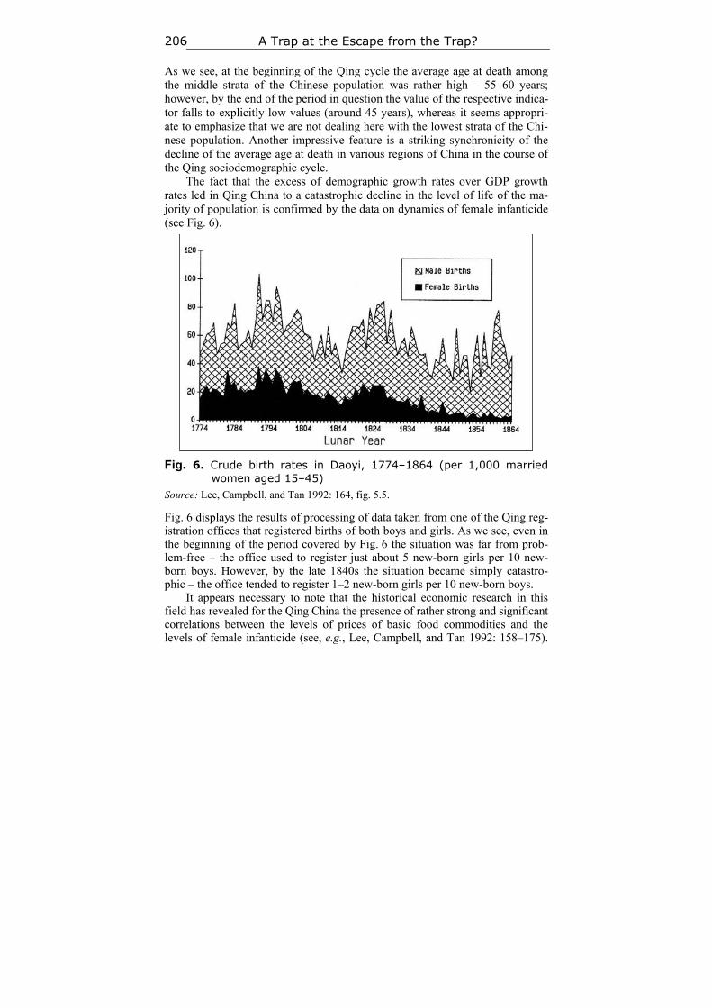
A Trap at the Escape from the Trap? 206
As we see, at the beginning of the Qing cycle the average age at death among the middle strata of the Chinese population was rather high – 55–60 years; however, by the end of the period in question the value of the respective indica-tor falls to explicitly low values (around 45 years), whereas it seems appropri-ate to emphasize that we are not dealing here with the lowest strata of the Chi-nese population. Another impressive feature is a striking synchronicity of the decline of the average age at death in various regions of China in the course of the Qing sociodemographic cycle.
The fact that the excess of demographic growth rates over GDP growth rates led in Qing China to a catastrophic decline in the level of life of the ma-jority of population is confirmed by the data on dynamics of female infanticide (see Fig. 6).
Fig. 6. Crude birth rates in Daoyi, 1774–1864 (per 1,000 married women aged 15–45)
Source: Lee, Campbell, and Tan 1992: 164, fig. 5.5.
Fig. 6 displays the results of processing of data taken from one of the Qing reg-istration offices that registered births of both boys and girls. As we see, even in the beginning of the period covered by Fig. 6 the situation was far from prob-lem-free – the office used to register just about 5 new-born girls per 10 new-born boys. However, by the late 1840s the situation became simply catastro-phic – the office tended to register 1–2 new-born girls per 10 new-born boys.
It appears necessary to note that the historical economic research in this field has revealed for the Qing China the presence of rather strong and significant correlations between the levels of prices of basic food commodities and the levels of female infanticide (see, e.g., Lee, Campbell, and Tan 1992: 158–175).
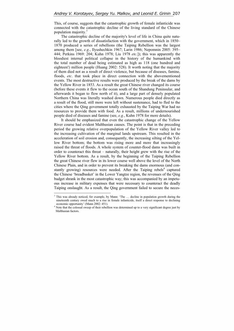
Andrey V. Korotayev, Sergey Yu. Malkov, and Leonid E. Grinin 207
This, of course, suggests that the catastrophic growth of female infanticide was connected with the catastrophic decline of the living standard of the Chinese population majority.3
The catastrophic decline of the majority's level of life in China quite natu-rally led to the growth of dissatisfaction with the government, which in 1850–1870 produced a series of rebellions (the Taiping Rebellion was the largest among them [see, e.g., Ilyushechkin 1967; Larin 1986; Nepomnin 2005: 395–444; Perkins 1969: 204; Kuhn 1978; Liu 1978 etc.]); this was apparently the bloodiest internal political collapse in the history of the humankind with the total number of dead being estimated as high as 118 (one hundred and eighteen!) million people (Huang 2002: 528). It worth noting that the majority of them died not as a result of direct violence, but because of diseases, famine, floods, etc. that took place in direct connection with the abovementioned events. The most destructive results were produced by the break of the dams by the Yellow River in 1853. As a result the great Chinese river changed its course (before these events it flew to the ocean south of the Shandung Peninsular, and afterwards it began to flow north of it), and a large part of densely populated Northern China was literally washed down. Numerous people died directly as a result of the flood, still more were left without sustenance, had to fled to the cities where the Qing government totally exhausted by the Taiping War had no resources to provide them with food. As a result, millions of undernourished people died of diseases and famine (see, e.g., Kuhn 1978 for more details).
It should be emphasized that even the catastrophic change of the Yellow River course had evident Malthusian causes. The point is that in the preceding period the growing relative overpopulation of the Yellow River valley led to the increasing cultivation of the marginal lands upstream. This resulted in the acceleration of soil erosion and, consequently, the increasing silting of the Yel-low River bottom; the bottom was rising more and more that increasingly raised the threat of floods. A whole system of counter-flood dams was built in order to counteract this threat – naturally, their height grew with the rise of the Yellow River bottom. As a result, by the beginning of the Taiping Rebellion the great Chinese river flew in its lower course well above the level of the North Chinese Plain, and in order to prevent its breaking the dams enormous (and con-stantly growing) resources were needed. After the Taiping rebels4 captured the Chinese ‘breadbasket’ in the Lower Yangtze region, the revenues of the Qing budget shrank in the most catastrophic way; this was accompanied by an impetu-ous increase in military expenses that were necessary to counteract the deadly Taiping onslaught. As a result, the Qing government failed to secure the neces- 3 This was already noticed, for example, by Mann: ‘The … decline in population growth during the
nineteenth century owed much to a rise in female infanticide, itself a direct response to declining economic opportunity’ (Mann 2002: 451).
4 Note that the colossal sweep of their rebellion was determined up to a very significant degree just by Malthusian factors.
A Trap at the Escape from the Trap? 208
sary (and very costly) support of the extremely complex counter-flood system, and the catastrophic break of the dams by the Yellow River became inevitable (see Korotayev, Malkov, and Khaltourina 2006b: ch. 2 for more details).
Note that Malthus himself considered warfare (including, naturally, inter-nal warfare) as one of the most important results of overpopulation (in addition to epidemics and famines). What is more, he regarded wars, epidemics, and famines (and all of these were observed in China in 1850–1870) as so-called ‘positive checks’ that checked overpopulation in pre-industrial systems (Mal-thus 1978 [1798]). Thus, in pre-industrial societies bloody political upheavals frequently turned out to be a result of the respective social systems being caught in the Malthusian trap.
By now the students of social systems entrapped in the Malthusian trap have a rather significant number of mathematical models of political-demographic dynamics of such social systems describing the development of bloody political upheavals at the phase of socio-demographic collapse of pre-industrial political-demographic cycles (see, e.g., Korotayev and Khaltourina 2006; Korotayev, Malkov, and Khaltourina 2006b; Usher 1989; Chu and Lee 1994; Malkov 2009; Komlos and Nefedov 2002; Turchin 2003, 2005a, 2005b; Nefedov 2004; Turchin and Nefedov 2009; Turchin and Korotayev 2006 etc.).
Demographic transition and the increase in agricultural productivity due to major technological advances in the recent centuries (see, e.g., Grinin 2006) allowed most states to escape the Malthusian trap. The first phase of the demo-graphic transition is characterized by a decline in mortality due to improved nutrition, sanitation, advancement and spread of modern medical technologies, etc. This leads to the acceleration of population growth. In the second phase of demographic transition, the development of medicine in combination with other processes (especially with mass education among women) leads to a wide-spread use of family planning technologies and, as a result, to a decrease of population growth rates (see, e.g., Chesnais 1992; Korotayev, Malkov, and Khaltourina 2006a).
However, these modernization processes started later in Sub-Saharan Af-rica than in the rest of the world; and even in the recent decades the Malthusian trap tended to produce state breakdowns in this region.
For example, in the period preceding the fall of Mengistu Haile Mariam's regime, from 1981 to 1991, Ethiopia's GDP grew by 12.5 %, but during the same period the population grew by 40 %. As a result, GDP per capita fell from very low $608 to catastrophic $500. Another dramatic fall occurred in per cap-ita calorie intake: 1831 kcal/day in 1981 was already very low, 1657 in 1991 was below physiological minimum (see Table 1).
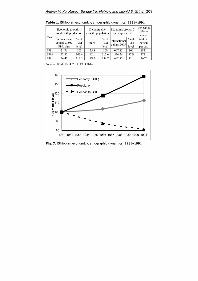
Andrey V. Korotayev, Sergey Yu. Malkov, and Leonid E. Grinin 209
Table 1. Ethiopian economic-demographic dynamics, 1981–1991
Economic growth 1: total GDP production
Demographic growth: population
Economic growth 2:per capita GDP
Per capita calorie intake
Year international dollars 2005,
PPP, blns
% of 1981 level
mlns % of 1981 level
internationaldollars 2005
% of 1981 level
kcal per person per day
1981 21.76 100 35.8 100 607.85 100 1831 1986 22.50 103.4 42.1 117.6 534.24 87.9 1711 1991 24.47 112.5 49.7 138.7 492.85 81.1 1657
Sources: World Bank 2014; FAO 2014.
80
90
100
110
120
130
140
1981 1982 1983 1984 1985 1986 1987 1988 1989 1990 1991
100
= 1
981
leve
l
Economy (GDP)
Population
Per capita GDP
Fig. 7. Ethiopian economic-demographic dynamics, 1981–1991
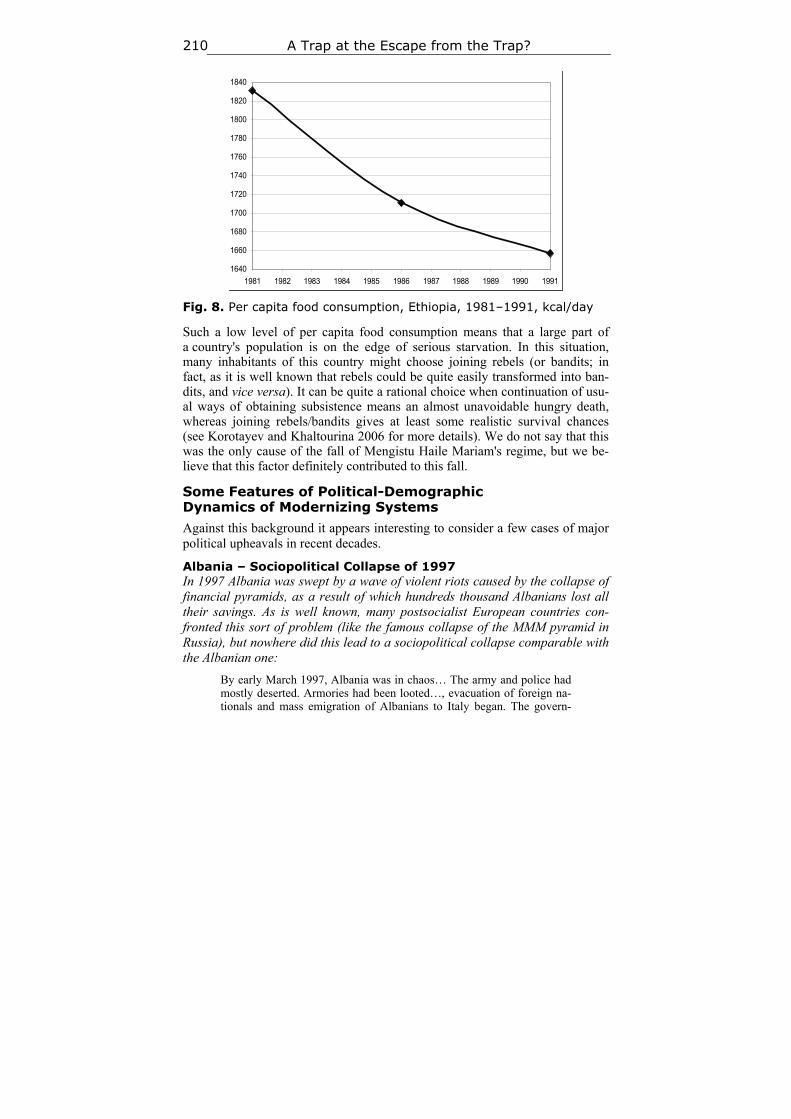
A Trap at the Escape from the Trap? 210
Fig. 8. Per capita food consumption, Ethiopia, 1981–1991, kcal/day
Such a low level of per capita food consumption means that a large part of a country's population is on the edge of serious starvation. In this situation, many inhabitants of this country might choose joining rebels (or bandits; in fact, as it is well known that rebels could be quite easily transformed into ban-dits, and vice versa). It can be quite a rational choice when continuation of usu-al ways of obtaining subsistence means an almost unavoidable hungry death, whereas joining rebels/bandits gives at least some realistic survival chances (see Korotayev and Khaltourina 2006 for more details). We do not say that this was the only cause of the fall of Mengistu Haile Mariam's regime, but we be-lieve that this factor definitely contributed to this fall.
Some Features of Political-Demographic Dynamics of Modernizing Systems
Against this background it appears interesting to consider a few cases of major political upheavals in recent decades.
Albania – Sociopolitical Collapse of 1997 In 1997 Albania was swept by a wave of violent riots caused by the collapse of financial pyramids, as a result of which hundreds thousand Albanians lost all their savings. As is well known, many postsocialist European countries con-fronted this sort of problem (like the famous collapse of the MMM pyramid in Russia), but nowhere did this lead to a sociopolitical collapse comparable with the Albanian one:
By early March 1997, Albania was in chaos… The army and police had mostly deserted. Armories had been looted…, evacuation of foreign na-tionals and mass emigration of Albanians to Italy began. The govern-
1640
1660
1680
1700
1720
1740
1760
1780
1800
1820
1840
1981 1982 1983 1984 1985 1986 1987 1988 1989 1990 1991
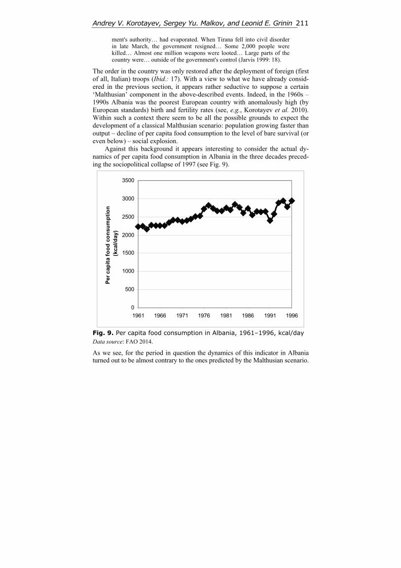
Andrey V. Korotayev, Sergey Yu. Malkov, and Leonid E. Grinin 211
ment's authority… had evaporated. When Tirana fell into civil disorder in late March, the government resigned… Some 2,000 people were killed… Almost one million weapons were looted… Large parts of the country were… outside of the government's control (Jarvis 1999: 18).
The order in the country was only restored after the deployment of foreign (first of all, Italian) troops (Ibid.: 17). With a view to what we have already consid-ered in the previous section, it appears rather seductive to suppose a certain ‘Malthusian’ component in the above-described events. Indeed, in the 1960s – 1990s Albania was the poorest European country with anomalously high (by European standards) birth and fertility rates (see, e.g., Korotayev et al. 2010). Within such a context there seem to be all the possible grounds to expect the development of a classical Malthusian scenario: population growing faster than output – decline of per capita food consumption to the level of bare survival (or even below) – social explosion.
Against this background it appears interesting to consider the actual dy-namics of per capita food consumption in Albania in the three decades preced-ing the sociopolitical collapse of 1997 (see Fig. 9).
0
500
1000
1500
2000
2500
3000
3500
1961 1966 1971 1976 1981 1986 1991 1996
Per
cap
ita
foo
d c
on
sum
pti
on
(
kcal
/day
)
Fig. 9. Per capita food consumption in Albania, 1961–1996, kcal/day
Data source: FAO 2014.
As we see, for the period in question the dynamics of this indicator in Albania turned out to be almost contrary to the ones predicted by the Malthusian scenario.
A Trap at the Escape from the Trap? 212
Still in the early 1960s in Albania the problem of malnutrition was very serious and the average per capita food consumption was below the norm of 2300–2400 kcal/day recommended by the WHO (see, e.g., Naiken 2002).
However, in the 1960s and 1970s Albania managed to achieve evident suc-cesses in the solution of the food problem; in the late 1960s – early 1970s in this country the per capita food consumption exceeded the norm recommended by the WHO – and afterwards it has never dropped below it. In the late 1970s and early 1980s the growth rate of this indicator slowed down, and in 1983–1991 a certain trend towards its decline was observed, which, of course, reflects very serious economic difficulties that were experienced by Albania in the last years of the ‘communist’ period of its history (see, e.g., Sandstrom and Sjöberg 1991). However, even in 1991 (the hardest year in Albania) per capita food consumption did not drop below the norm recommended by the WHO. On the other hand, after 1991 Albania managed to achieve new successes in solving the food problem, and in 1993–1996 per capita food consumption in Albania reached record values for the whole Albanian history; by 1997 it was closer to what would be more appropriately called ‘overeating’ rather than ‘undernour-ishment’ level.
In any case, we may maintain with a high degree of confidence that with respect to Albania in 1961–1997 it appear impossible to speak about anything like a drop of per capita food consumption to the level of bare survival as a result of the population growing faster than output. It appears much more appropriate to say that these were precisely those years when Albania managed to escape quite successfully from the Malthusian trap.5
South Korea – The 1980 Kwangju Uprising After the end of the Korean War the largest popular uprising in South Korea took place in 1980 in the city of Kwangju (with 300 thousand participants, about 2000 dead, 5 divisions of regular army taking part in the suppression of the rebellion, etc.). This uprising was accompanied by a series of popular riots in neighboring cities (Lewis 2002).
Against this background, the dynamics of per capita food consumption in South Korea in the two decades preceding the abovementioned popular rebel-lion looks rather noteworthy (see Fig. 10).
5 Naturally, the 1997 sociopolitical collapse led to a certain decline in the average per capita food
consumption (below 2700 kcal per day), which was still above the level recommended by the WHO; whereas later the growth of this indicator resumed (FAO 2014).
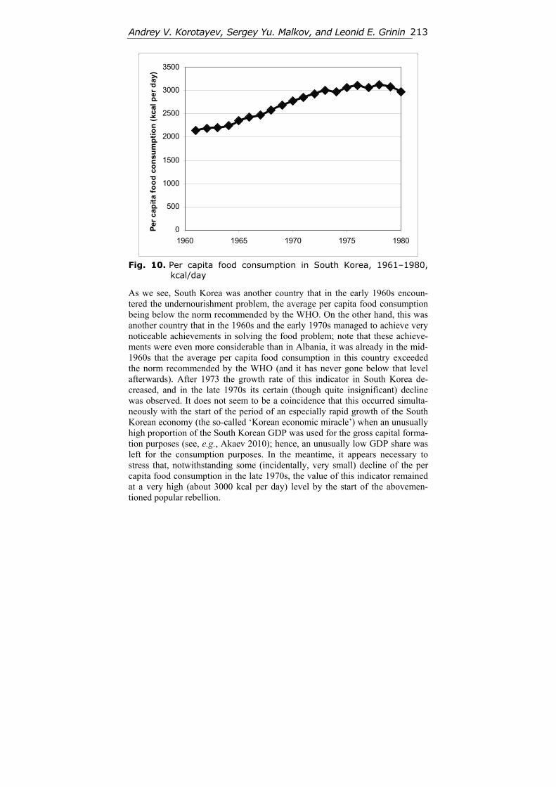
Andrey V. Korotayev, Sergey Yu. Malkov, and Leonid E. Grinin 213
0
500
1000
1500
2000
2500
3000
3500
1960 1965 1970 1975 1980
Per
cap
ita
foo
d c
on
sum
pti
on
(kc
al p
er d
ay)
Fig. 10. Per capita food consumption in South Korea, 1961–1980,
kcal/day
As we see, South Korea was another country that in the early 1960s encoun-tered the undernourishment problem, the average per capita food consumption being below the norm recommended by the WHO. On the other hand, this was another country that in the 1960s and the early 1970s managed to achieve very noticeable achievements in solving the food problem; note that these achieve-ments were even more considerable than in Albania, it was already in the mid-1960s that the average per capita food consumption in this country exceeded the norm recommended by the WHO (and it has never gone below that level afterwards). After 1973 the growth rate of this indicator in South Korea de-creased, and in the late 1970s its certain (though quite insignificant) decline was observed. It does not seem to be a coincidence that this occurred simulta-neously with the start of the period of an especially rapid growth of the South Korean economy (the so-called ‘Korean economic miracle’) when an unusually high proportion of the South Korean GDP was used for the gross capital forma-tion purposes (see, e.g., Akaev 2010); hence, an unusually low GDP share was left for the consumption purposes. In the meantime, it appears necessary to stress that, notwithstanding some (incidentally, very small) decline of the per capita food consumption in the late 1970s, the value of this indicator remained at a very high (about 3000 kcal per day) level by the start of the abovemen-tioned popular rebellion.
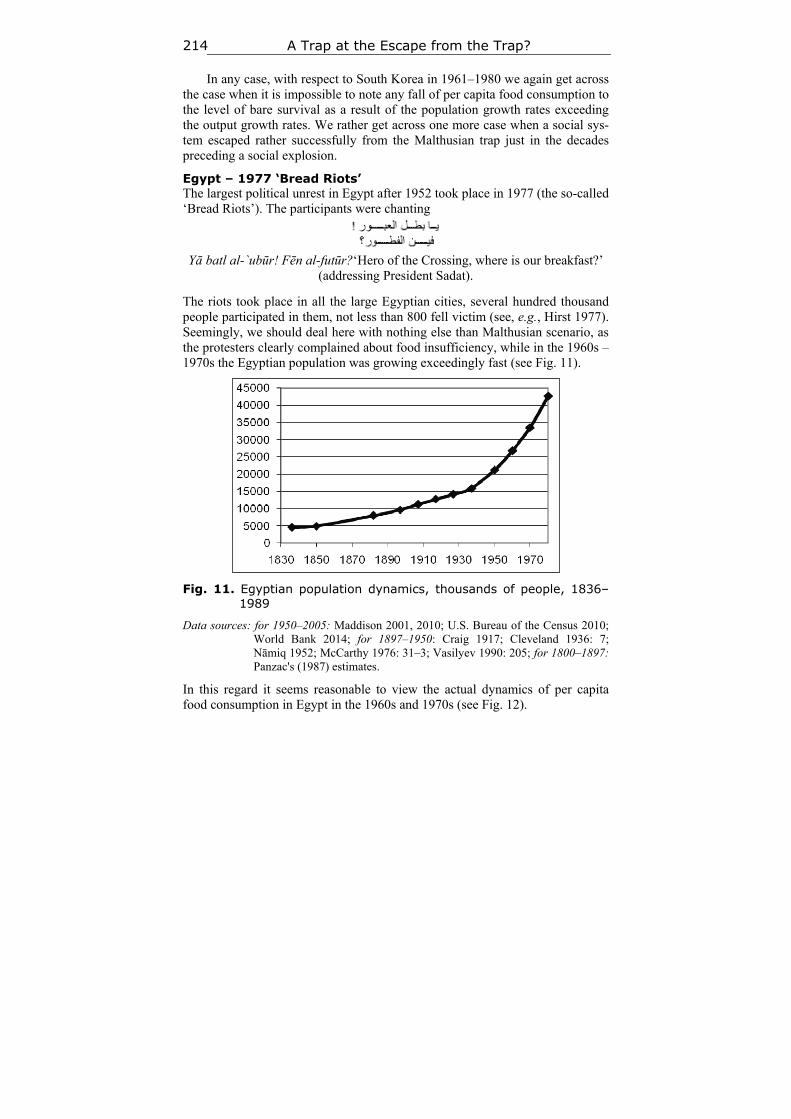
A Trap at the Escape from the Trap? 214
In any case, with respect to South Korea in 1961–1980 we again get across the case when it is impossible to note any fall of per capita food consumption to the level of bare survival as a result of the population growth rates exceeding the output growth rates. We rather get across one more case when a social sys-tem escaped rather successfully from the Malthusian trap just in the decades preceding a social explosion.
Egypt – 1977 ‘Bread Riots’ The largest political unrest in Egypt after 1952 took place in 1977 (the so-called ‘Bread Riots’). The participants were chanting
Yā batl al-`ubūr! Fēn al-futūr?‘Hero of the Crossing, where is our breakfast?’
(addressing President Sadat).
The riots took place in all the large Egyptian cities, several hundred thousand people participated in them, not less than 800 fell victim (see, e.g., Hirst 1977). Seemingly, we should deal here with nothing else than Malthusian scenario, as the protesters clearly complained about food insufficiency, while in the 1960s – 1970s the Egyptian population was growing exceedingly fast (see Fig. 11).
Fig. 11. Egyptian population dynamics, thousands of people, 1836–1989
Data sources: for 1950–2005: Maddison 2001, 2010; U.S. Bureau of the Census 2010; World Bank 2014; for 1897–1950: Craig 1917; Cleveland 1936: 7; Nāmiq 1952; McCarthy 1976: 31–3; Vasilyev 1990: 205; for 1800–1897: Panzac's (1987) estimates.
In this regard it seems reasonable to view the actual dynamics of per capita food consumption in Egypt in the 1960s and 1970s (see Fig. 12).
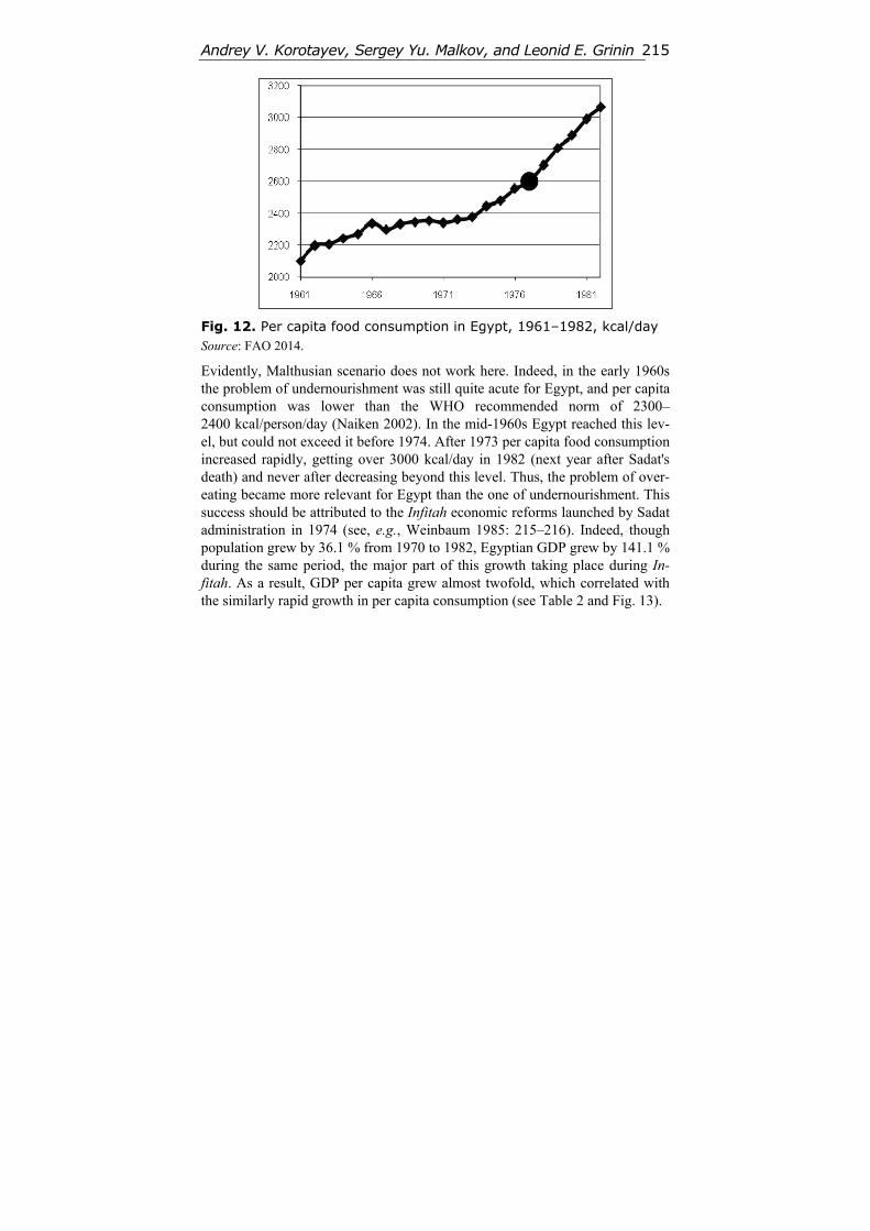
Andrey V. Korotayev, Sergey Yu. Malkov, and Leonid E. Grinin 215
Fig. 12. Per capita food consumption in Egypt, 1961–1982, kcal/day
Source: FAO 2014.
Evidently, Malthusian scenario does not work here. Indeed, in the early 1960s the problem of undernourishment was still quite acute for Egypt, and per capita consumption was lower than the WHO recommended norm of 2300– 2400 kcal/person/day (Naiken 2002). In the mid-1960s Egypt reached this lev-el, but could not exceed it before 1974. After 1973 per capita food consumption increased rapidly, getting over 3000 kcal/day in 1982 (next year after Sadat's death) and never after decreasing beyond this level. Thus, the problem of over-eating became more relevant for Egypt than the one of undernourishment. This success should be attributed to the Infitah economic reforms launched by Sadat administration in 1974 (see, e.g., Weinbaum 1985: 215–216). Indeed, though population grew by 36.1 % from 1970 to 1982, Egyptian GDP grew by 141.1 % during the same period, the major part of this growth taking place during In-fitah. As a result, GDP per capita grew almost twofold, which correlated with the similarly rapid growth in per capita consumption (see Table 2 and Fig. 13).
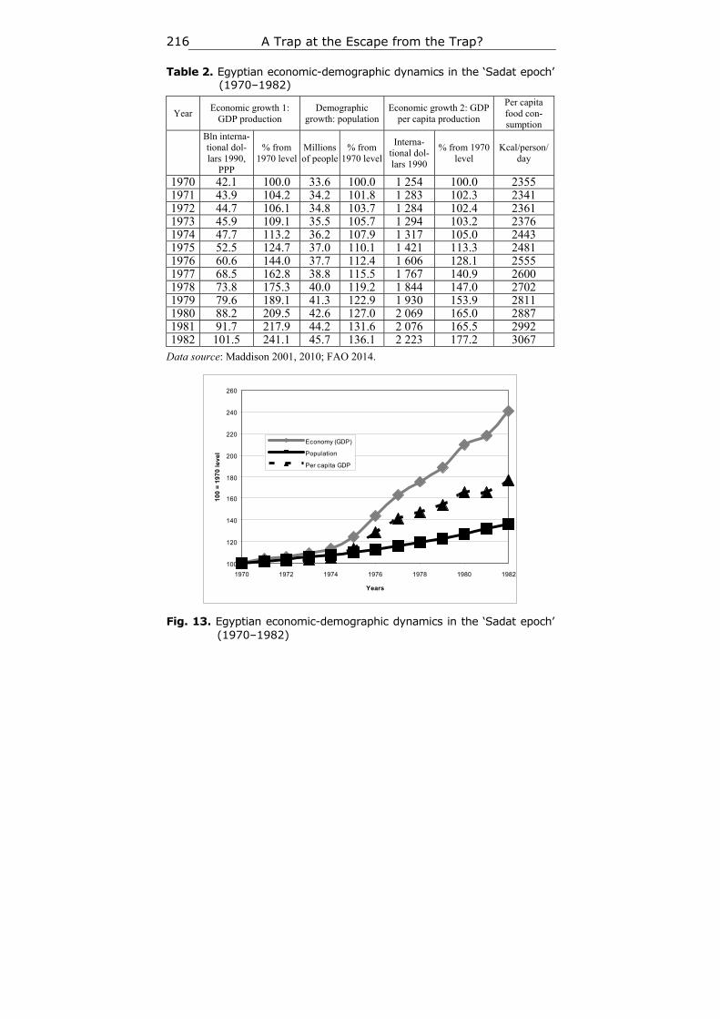
A Trap at the Escape from the Trap? 216
Table 2. Egyptian economic-demographic dynamics in the ‘Sadat epoch’ (1970–1982)
Year Economic growth 1:
GDP production Demographic
growth: populationEconomic growth 2: GDP
per capita production
Per capita food con-sumption
Bln interna-tional dol-lars 1990,
PPP
% from 1970 level
Millions of people
% from 1970 level
Interna-tional dol-lars 1990
% from 1970 level
Kcal/person/ day
1970 42.1 100.0 33.6 100.0 1 254 100.0 2355 1971 43.9 104.2 34.2 101.8 1 283 102.3 2341 1972 44.7 106.1 34.8 103.7 1 284 102.4 2361 1973 45.9 109.1 35.5 105.7 1 294 103.2 2376 1974 47.7 113.2 36.2 107.9 1 317 105.0 2443 1975 52.5 124.7 37.0 110.1 1 421 113.3 2481 1976 60.6 144.0 37.7 112.4 1 606 128.1 2555 1977 68.5 162.8 38.8 115.5 1 767 140.9 2600 1978 73.8 175.3 40.0 119.2 1 844 147.0 2702 1979 79.6 189.1 41.3 122.9 1 930 153.9 2811 1980 88.2 209.5 42.6 127.0 2 069 165.0 2887 1981 91.7 217.9 44.2 131.6 2 076 165.5 2992 1982 101.5 241.1 45.7 136.1 2 223 177.2 3067
Data source: Maddison 2001, 2010; FAO 2014.
100
120
140
160
180
200
220
240
260
1970 1972 1974 1976 1978 1980 1982
Years
10
0 =
19
70
le
ve
l
Economy (GDP)
Population
Per capita GDP
Fig. 13. Egyptian economic-demographic dynamics in the ‘Sadat epoch’ (1970–1982)
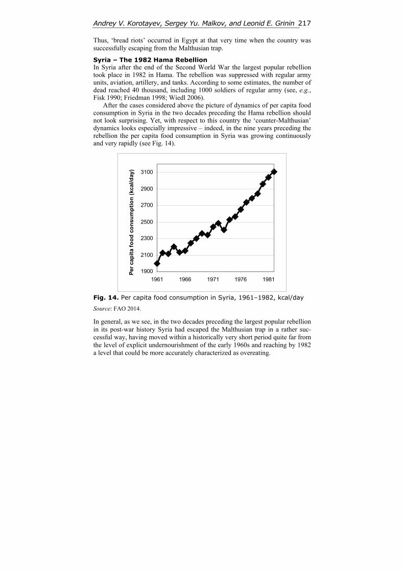
Andrey V. Korotayev, Sergey Yu. Malkov, and Leonid E. Grinin 217
Thus, ‘bread riots’ occurred in Egypt at that very time when the country was successfully escaping from the Malthusian trap.
Syria – The 1982 Hama Rebellion In Syria after the end of the Second World War the largest popular rebellion took place in 1982 in Hama. The rebellion was suppressed with regular army units, aviation, artillery, and tanks. According to some estimates, the number of dead reached 40 thousand, including 1000 soldiers of regular army (see, e.g., Fisk 1990; Friedman 1998; Wiedl 2006).
After the cases considered above the picture of dynamics of per capita food consumption in Syria in the two decades preceding the Hama rebellion should not look surprising. Yet, with respect to this country the ‘counter-Malthusian’ dynamics looks especially impressive – indeed, in the nine years preceding the rebellion the per capita food consumption in Syria was growing continuously and very rapidly (see Fig. 14).
1900
2100
2300
2500
2700
2900
3100
1961 1966 1971 1976 1981
Per
cap
ita
foo
d c
on
sum
pti
on
(kc
al/d
ay)
Fig. 14. Per capita food consumption in Syria, 1961–1982, kcal/day
Source: FAO 2014.
In general, as we see, in the two decades preceding the largest popular rebellion in its post-war history Syria had escaped the Malthusian trap in a rather suc-cessful way, having moved within a historically very short period quite far from the level of explicit undernourishment of the early 1960s and reaching by 1982 a level that could be more accurately characterized as overeating.
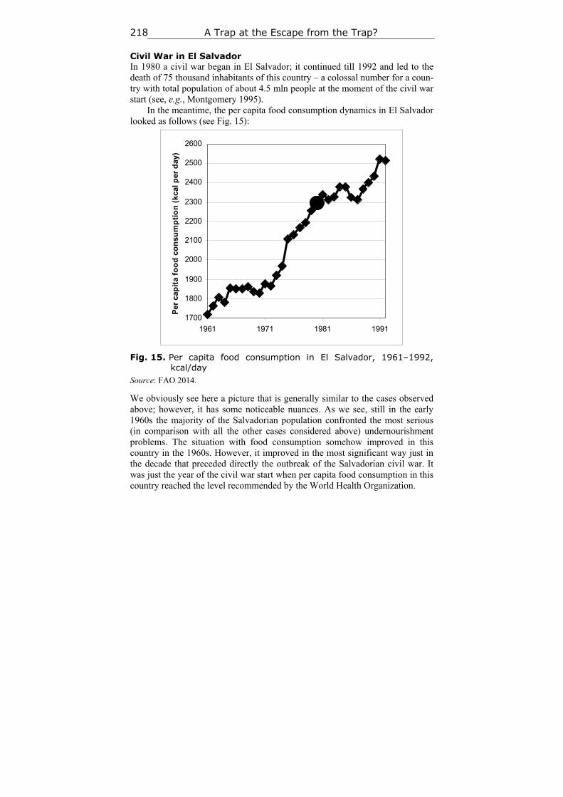
A Trap at the Escape from the Trap? 218
Civil War in El Salvador In 1980 a civil war began in El Salvador; it continued till 1992 and led to the death of 75 thousand inhabitants of this country – a colossal number for a coun-try with total population of about 4.5 mln people at the moment of the civil war start (see, e.g., Montgomery 1995).
In the meantime, the per capita food consumption dynamics in El Salvador looked as follows (see Fig. 15):
1700
1800
1900
2000
2100
2200
2300
2400
2500
2600
1961 1971 1981 1991
Per
cap
ita
foo
d c
on
sum
pti
on
(kc
al p
er d
ay)
Fig. 15. Per capita food consumption in El Salvador, 1961–1992,
kcal/day Source: FAO 2014.
We obviously see here a picture that is generally similar to the cases observed above; however, it has some noticeable nuances. As we see, still in the early 1960s the majority of the Salvadorian population confronted the most serious (in comparison with all the other cases considered above) undernourishment problems. The situation with food consumption somehow improved in this country in the 1960s. However, it improved in the most significant way just in the decade that preceded directly the outbreak of the Salvadorian civil war. It was just the year of the civil war start when per capita food consumption in this country reached the level recommended by the World Health Organization.
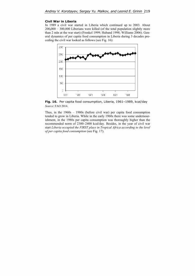
Andrey V. Korotayev, Sergey Yu. Malkov, and Leonid E. Grinin 219
Civil War in Liberia In 1989 a civil war started in Liberia which continued up to 2003. About 200,000 – 300,000 Liberians were killed (of the total population slightly more than 2 mln at the war start) (Frenkel 1999; Huband 1998; Williams 2006). Gen-eral dynamics of per capita food consumption in Liberia during 3 decades pre-ceding the civil war looked as follows (see Fig. 16):
Fig. 16. Per capita food consumption, Liberia, 1961–1989, kcal/day
Source: FAO 2014.
Thus, in the 1960s – 1980s (before civil war) per capita food consumption tended to grow in Liberia. While in the early 1960s there was some undernour-ishment, in the 1980s per capita consumption was thoroughly higher than the recommended norm of 2300–2400 kcal/day. Besides, in the year of civil war start Liberia occupied the FIRST place in Tropical Africa according to the level of per capita food consumption (see Fig. 17).
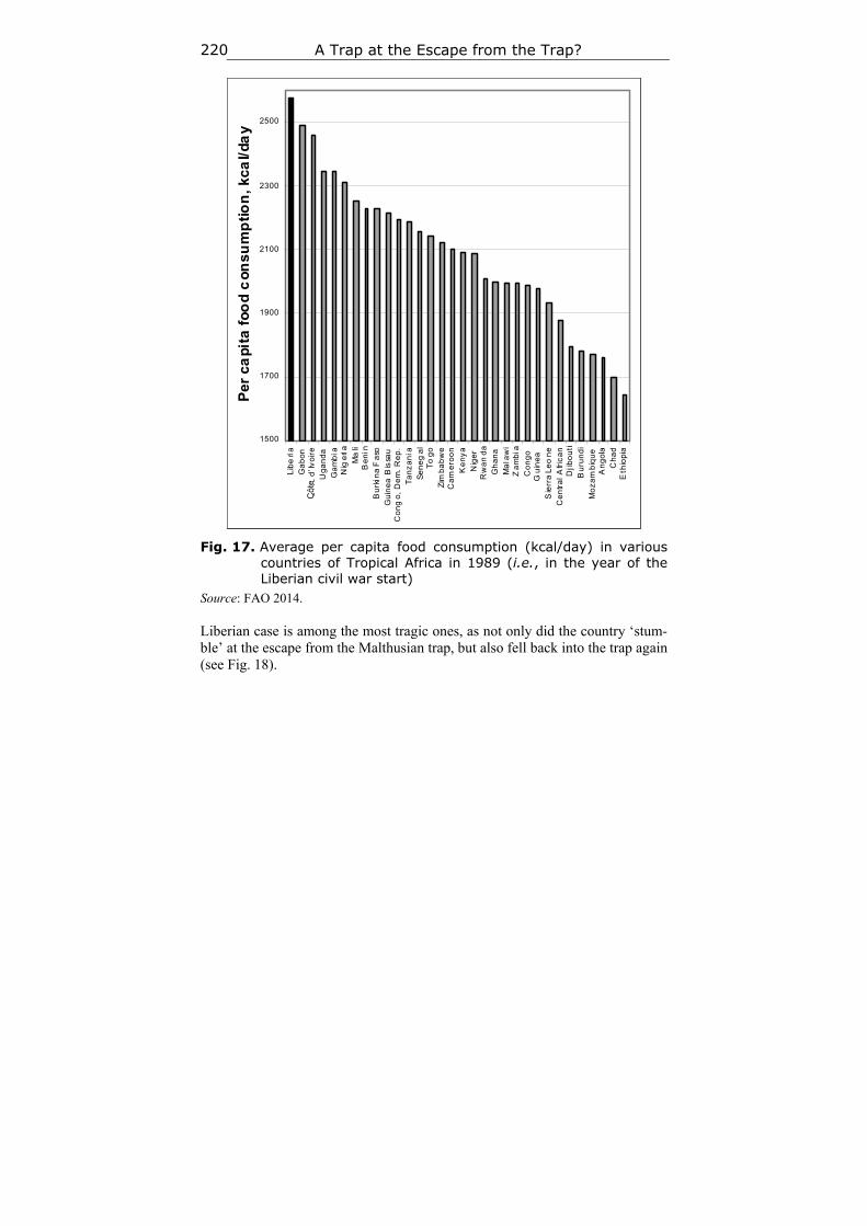
A Trap at the Escape from the Trap? 220
Fig. 17. Average per capita food consumption (kcal/day) in various countries of Tropical Africa in 1989 (i.e., in the year of the Liberian civil war start)
Source: FAO 2014. Liberian case is among the most tragic ones, as not only did the country ‘stum-ble’ at the escape from the Malthusian trap, but also fell back into the trap again (see Fig. 18).
1500
1700
1900
2100
2300
2500
Lib
eri
a
Ga
bo
nC
?te
d’I
vo
ire
Ug
an
da
Ga
mb
iaN
ige
ria
Ma
liB
en
in
Bu
rkin
a F
aso
Gu
ine
a B
issa
uC
on
go
, D
em
. R
ep
.
Ta
nz
an
ia
Se
ne
ga
lT
og
o
Zim
ba
bw
eC
am
ero
on
Ke
ny
a
Nig
er
Rw
an
da
Gh
an
a
Ma
law
iZ
am
bia
Co
ng
o
Gu
ine
a
Sie
rra
Le
on
e
Ce
ntr
al
Afr
ica
nD
jib
ou
ti
Bu
run
di
Mo
za
mb
iqu
eA
ng
ola
Ch
ad
Eth
iop
ia
Per
ca
pita
foo
d c
onsu
mp
tion
, kca
l/da
y
Cô
te
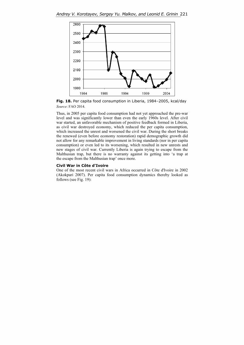
Andrey V. Korotayev, Sergey Yu. Malkov, and Leonid E. Grinin 221
Fig. 18. Per capita food consumption in Liberia, 1984–2005, kcal/day
Source: FAO 2014.
Thus, in 2005 per capita food consumption had not yet approached the pre-war level and was significantly lower than even the early 1960s level. After civil war started, an unfavorable mechanism of positive feedback formed in Liberia, as civil war destroyed economy, which reduced the per capita consumption, which increased the unrest and worsened the civil war. During the short breaks the renewed (even before economy restoration) rapid demographic growth did not allow for any remarkable improvement in living standards (nor in per capita consumption) or even led to its worsening, which resulted in new unrests and new stages of civil war. Currently Liberia is again trying to escape from the Malthusian trap, but there is no warranty against its getting into ‘a trap at the escape from the Malthusian trap’ once more.
Civil War in Côte d'Ivoire One of the most recent civil wars in Africa occurred in Côte d'Ivoire in 2002 (Akokpari 2007). Per capita food consumption dynamics thereby looked as follows (see Fig. 19):
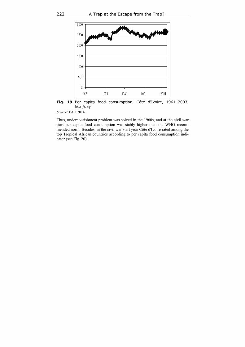
A Trap at the Escape from the Trap? 222
Fig. 19. Per capita food consumption, Côte d'Ivoire, 1961–2003, kcal/day
Source: FAO 2014.
Thus, undernourishment problem was solved in the 1960s, and at the civil war start per capita food consumption was stably higher than the WHO recom-mended norm. Besides, in the civil war start year Côte d'Ivoire rated among the top Tropical African countries according to per capita food consumption indi-cator (see Fig. 20).
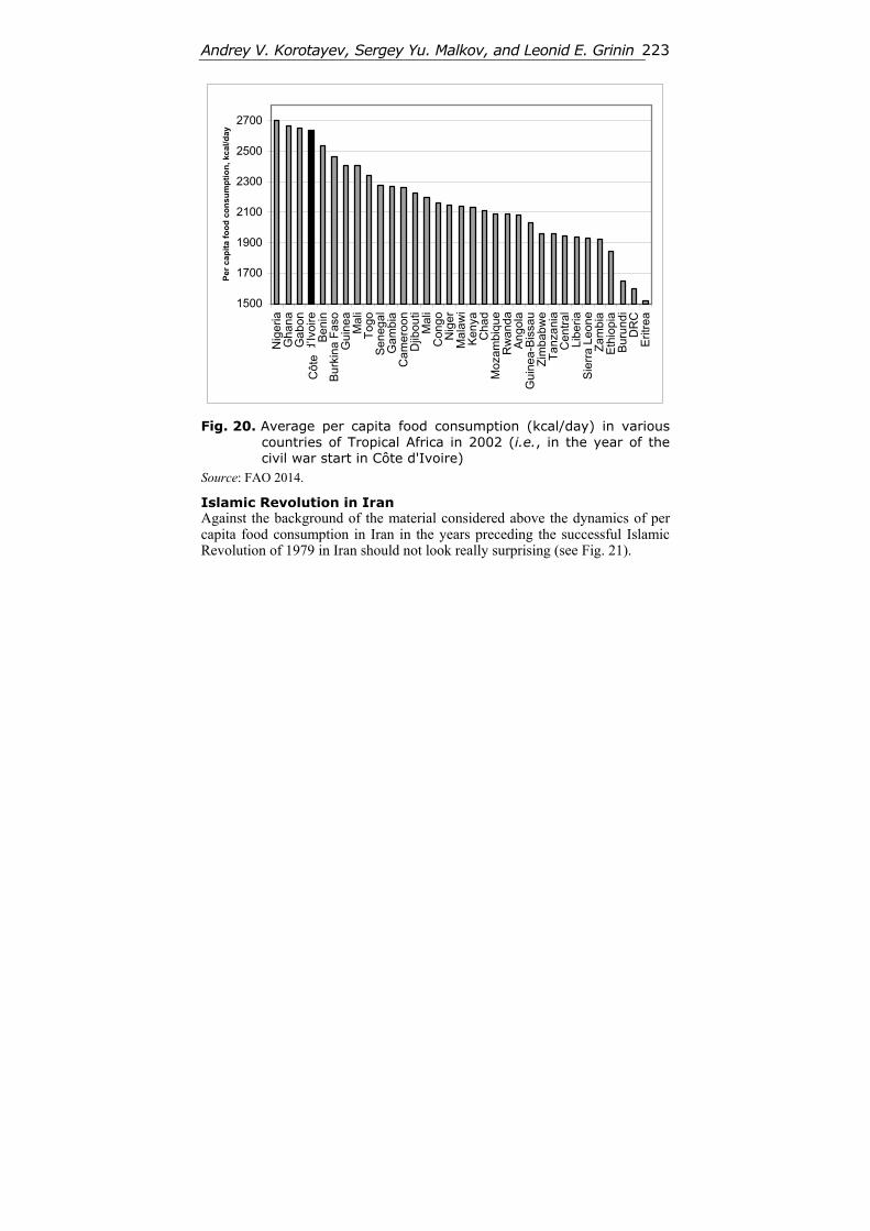
Andrey V. Korotayev, Sergey Yu. Malkov, and Leonid E. Grinin 223
1500
1700
1900
2100
2300
2500
2700
Nig
eri
aG
ha
na
Ga
bo
nC
ote
d’Iv
oire
Be
nin
Bu
rkin
a F
aso
Gu
ine
aM
ali
To
go
Se
ne
ga
lG
am
bia
Ca
me
roo
nD
jibo
uti
Ma
liC
on
go
Nig
er
Ma
law
iK
en
yaC
ha
dM
oza
mb
iqu
eR
wa
nd
aA
ng
ola
Gu
ine
a-B
issa
uZ
imb
ab
we
Ta
nza
nia
Ce
ntr
al
Lib
eri
aS
ierr
a L
eo
ne
Za
mb
iaE
thio
pia
Bu
run
di
DR
CE
ritre
a
Per
cap
ita
foo
d c
on
sum
pti
on
, kc
al/d
ay
Fig. 20. Average per capita food consumption (kcal/day) in various
countries of Tropical Africa in 2002 (i.e., in the year of the civil war start in Côte d'Ivoire)
Source: FAO 2014.
Islamic Revolution in Iran Against the background of the material considered above the dynamics of per capita food consumption in Iran in the years preceding the successful Islamic Revolution of 1979 in Iran should not look really surprising (see Fig. 21).
Côt
e
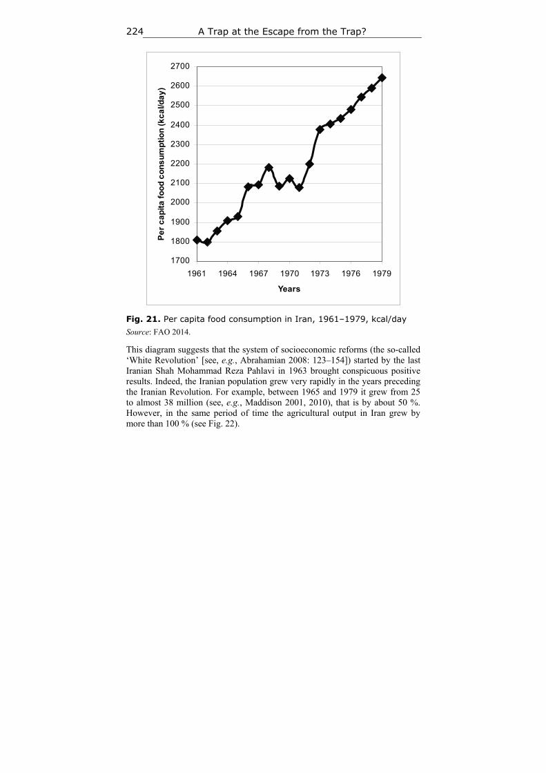
A Trap at the Escape from the Trap? 224
1700
1800
1900
2000
2100
2200
2300
2400
2500
2600
2700
1961 1964 1967 1970 1973 1976 1979
Years
Pe
r c
ap
ita
fo
od
co
ns
um
pti
on
(k
ca
l/da
y)
Fig. 21. Per capita food consumption in Iran, 1961–1979, kcal/day
Source: FAO 2014.
This diagram suggests that the system of socioeconomic reforms (the so-called ‘White Revolution’ [see, e.g., Abrahamian 2008: 123–154]) started by the last Iranian Shah Mohammad Reza Pahlavi in 1963 brought conspicuous positive results. Indeed, the Iranian population grew very rapidly in the years preceding the Iranian Revolution. For example, between 1965 and 1979 it grew from 25 to almost 38 million (see, e.g., Maddison 2001, 2010), that is by about 50 %. However, in the same period of time the agricultural output in Iran grew by more than 100 % (see Fig. 22).
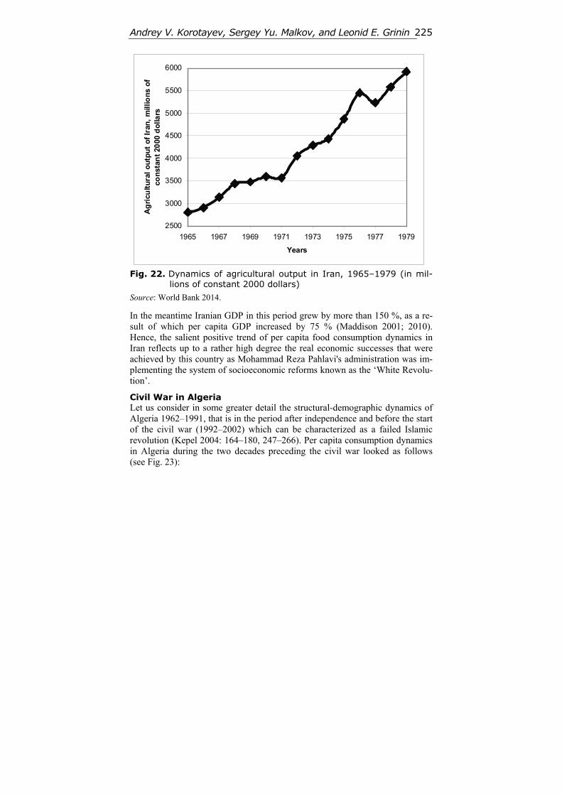
Andrey V. Korotayev, Sergey Yu. Malkov, and Leonid E. Grinin 225
2500
3000
3500
4000
4500
5000
5500
6000
1965 1967 1969 1971 1973 1975 1977 1979
Years
Ag
ricu
ltu
ral
ou
tpu
t o
f Ir
an,
mill
ion
s o
f co
nst
ant
2000
do
llars
Fig. 22. Dynamics of agricultural output in Iran, 1965–1979 (in mil-
lions of constant 2000 dollars)
Source: World Bank 2014.
In the meantime Iranian GDP in this period grew by more than 150 %, as a re-sult of which per capita GDP increased by 75 % (Maddison 2001; 2010). Hence, the salient positive trend of per capita food consumption dynamics in Iran reflects up to a rather high degree the real economic successes that were achieved by this country as Mohammad Reza Pahlavi's administration was im-plementing the system of socioeconomic reforms known as the ‘White Revolu-tion’.
Civil War in Algeria Let us consider in some greater detail the structural-demographic dynamics of Algeria 1962–1991, that is in the period after independence and before the start of the civil war (1992–2002) which can be characterized as a failed Islamic revolution (Kepel 2004: 164–180, 247–266). Per capita consumption dynamics in Algeria during the two decades preceding the civil war looked as follows (see Fig. 23):
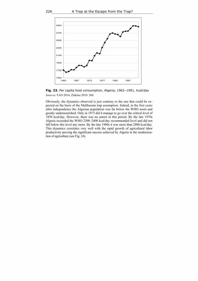
A Trap at the Escape from the Trap? 226
Fig. 23. Per capita food consumption, Algeria, 1962–1991, kcal/day
Sources: FAO 2014; Zinkina 2010: 260.
Obviously, the dynamics observed is just contrary to the one that could be ex-pected on the basis of the Malthusian trap assumption. Indeed, in the first years after independence the Algerian population was far below the WHO norm and greatly undernourished. Only in 1973 did it manage to go over the critical level of 1850 kcal/day. However, there was no unrest in this period. By the late 1970s Algeria exceeded the WHO 2300–2400 kcal/day recommended level and did not fall below this level any more. By the late 1980s it was more than 2800 kcal/day. This dynamics correlates very well with the rapid growth of agricultural labor productivity proving the significant success achieved by Algeria in the moderniza-tion of agriculture (see Fig. 24).
1500
1700
1900
2100
2300
2500
2700
2900
1962 1967 1972 1977 1982 1987
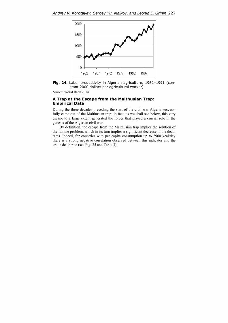
Andrey V. Korotayev, Sergey Yu. Malkov, and Leonid E. Grinin 227
Fig. 24. Labor productivity in Algerian agriculture, 1962–1991 (con-stant 2000 dollars per agricultural worker)
Source: World Bank 2014.
A Trap at the Escape from the Malthusian Trap: Empirical Data
During the three decades preceding the start of the civil war Algeria success-fully came out of the Malthusian trap; in fact, as we shall see below, this very escape to a large extent generated the forces that played a crucial role in the genesis of the Algerian civil war.
By definition, the escape from the Malthusian trap implies the solution of the famine problem, which in its turn implies a significant decrease in the death rates. Indeed, for countries with per capita consumption up to 2900 kcal/day there is a strong negative correlation observed between this indicator and the crude death rate (see Fig. 25 and Table 3).
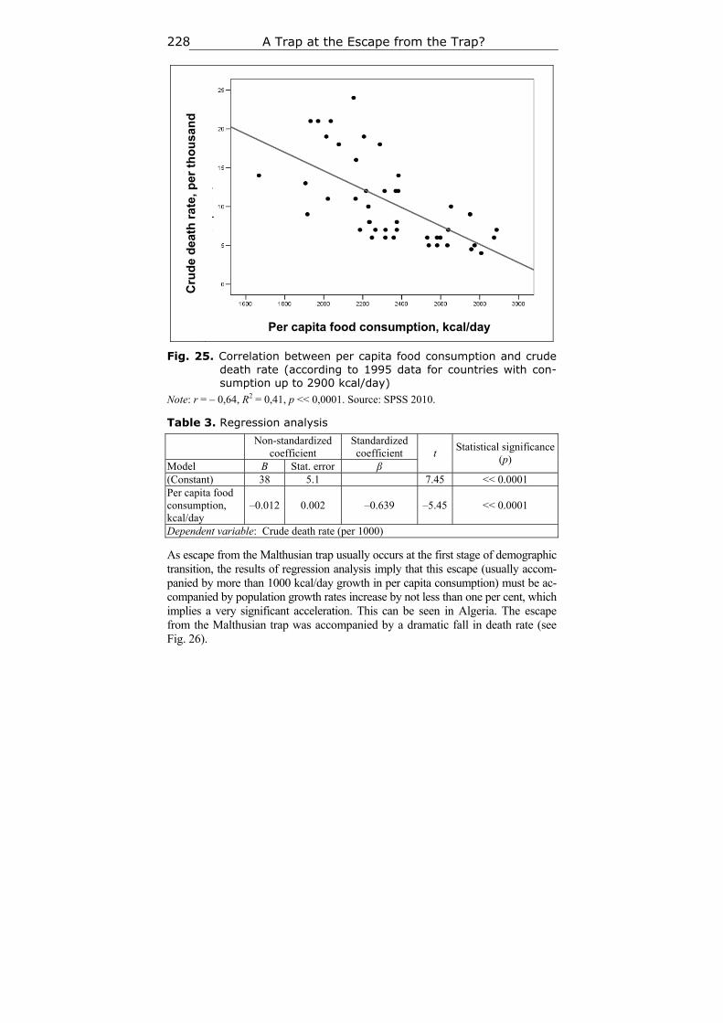
A Trap at the Escape from the Trap? 228
Cru
de
dea
th r
ate,
per
th
ou
san
d
Per capita food consumption, kcal/day
Fig. 25. Correlation between per capita food consumption and crude death rate (according to 1995 data for countries with con-sumption up to 2900 kcal/day)
Note: r = – 0,64, R2 = 0,41, p << 0,0001. Source: SPSS 2010.
Table 3. Regression analysis
Non-standardized coefficient
Standardized coefficient
Model B Stat. error β t
Statistical significance (p)
(Constant) 38 5.1 7.45 << 0.0001 Per capita food consumption, kcal/day
–0.012 0.002 –0.639 –5.45 << 0.0001
Dependent variable: Crude death rate (per 1000)
As escape from the Malthusian trap usually occurs at the first stage of demographic transition, the results of regression analysis imply that this escape (usually accom-panied by more than 1000 kcal/day growth in per capita consumption) must be ac-companied by population growth rates increase by not less than one per cent, which implies a very significant acceleration. This can be seen in Algeria. The escape from the Malthusian trap was accompanied by a dramatic fall in death rate (see Fig. 26).
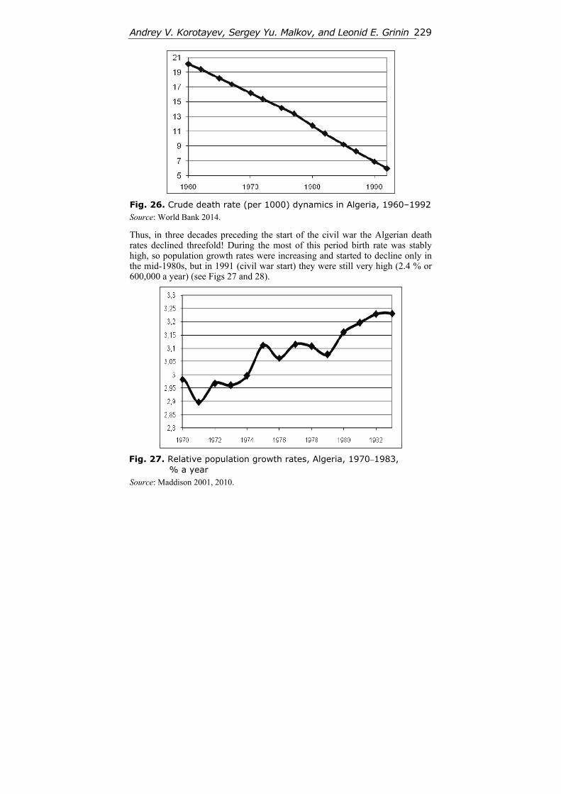
Andrey V. Korotayev, Sergey Yu. Malkov, and Leonid E. Grinin 229
Fig. 26. Crude death rate (per 1000) dynamics in Algeria, 1960–1992 Source: World Bank 2014.
Thus, in three decades preceding the start of the civil war the Algerian death rates declined threefold! During the most of this period birth rate was stably high, so population growth rates were increasing and started to decline only in the mid-1980s, but in 1991 (civil war start) they were still very high (2.4 % or 600,000 a year) (see Figs 27 and 28).
Fig. 27. Relative population growth rates, Algeria, 1970–1983, % a year
Source: Maddison 2001, 2010.
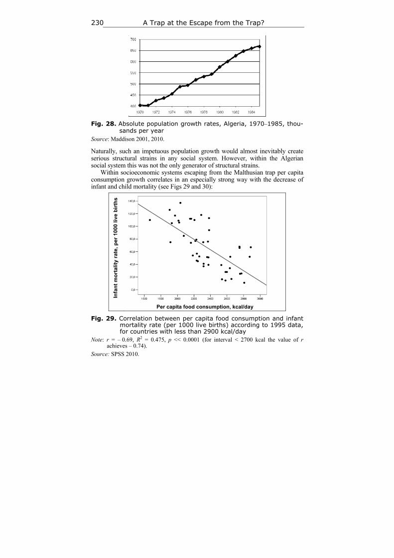
A Trap at the Escape from the Trap? 230
Fig. 28. Absolute population growth rates, Algeria, 1970–1985, thou-sands per year
Source: Maddison 2001, 2010.
Naturally, such an impetuous population growth would almost inevitably create serious structural strains in any social system. However, within the Algerian social system this was not the only generator of structural strains.
Within socioeconomic systems escaping from the Malthusian trap per capita consumption growth correlates in an especially strong way with the decrease of infant and child mortality (see Figs 29 and 30):
Infa
nt
mo
rtal
ity
rate
, per
10
00 li
ve b
irth
s
Per capita food consumption, kcal/day
Fig. 29. Correlation between per capita food consumption and infant mortality rate (per 1000 live births) according to 1995 data, for countries with less than 2900 kcal/day
Note: r = – 0.69, R2 = 0.475, p << 0.0001 (for interval < 2700 kcal the value of r achieves – 0.74).
Source: SPSS 2010.
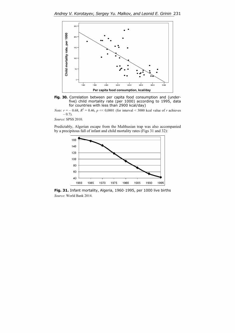
Andrey V. Korotayev, Sergey Yu. Malkov, and Leonid E. Grinin 231
Ch
ild m
ort
alit
y ra
te, p
er 1
000
Per capita food consumption, kcal/day
Fig. 30. Correlation between per capita food consumption and (under-five) child mortality rate (per 1000) according to 1995, data for countries with less than 2900 kcal/day)
Note: r = – 0.68, R2 = 0.46, p << 0,0001 (for interval < 3000 kcal value of r achieves – 0.7).
Source: SPSS 2010.
Predictably, Algerian escape from the Malthusian trap was also accompanied by a precipitous fall of infant and child mortality rates (Figs 31 and 32):
Fig. 31. Infant mortality, Algeria, 1960–1995, per 1000 live births Source: World Bank 2014.
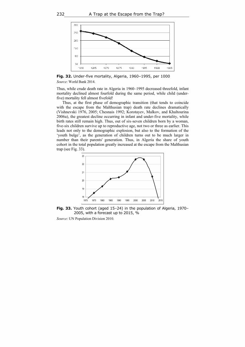
A Trap at the Escape from the Trap? 232
Fig. 32. Under-five mortality, Algeria, 1960–1995, per 1000 Source: World Bank 2014.
Thus, while crude death rate in Algeria in 1960–1995 decreased threefold, infant mortality declined almost fourfold during the same period, while child (under-five) mortality fell almost fivefold!
Thus, at the first phase of demographic transition (that tends to coincide with the escape from the Malthusian trap) death rate declines dramatically (Vishnevski 1976, 2005; Chesnais 1992; Korotayev, Malkov, and Khaltourina 2006a), the greatest decline occurring in infant and under-five mortality, while birth rates still remain high. Thus, out of six-seven children born by a woman, five-six children survive up to reproductive age, not two or three as earlier. This leads not only to the demographic explosion, but also to the formation of the ‘youth bulge’, as the generation of children turns out to be much larger in number than their parents' generation. Thus, in Algeria the share of youth cohort in the total population greatly increased at the escape from the Malthusian trap (see Fig. 33).
Fig. 33. Youth cohort (aged 15–24) in the population of Algeria, 1970–
2005, with a forecast up to 2015, %
Source: UN Population Division 2010.
18
19
20
21
22
23
1970 1975 1980 1985 1990 1995 2000 2005 2010 2015
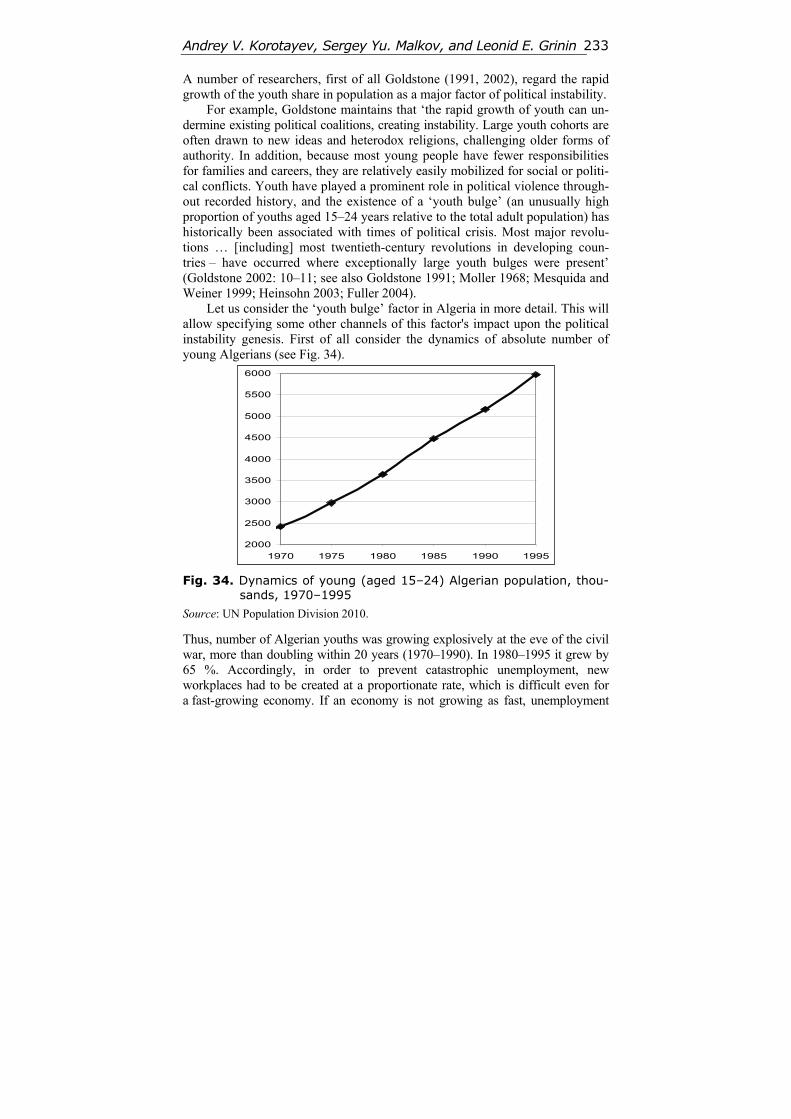
Andrey V. Korotayev, Sergey Yu. Malkov, and Leonid E. Grinin 233
A number of researchers, first of all Goldstone (1991, 2002), regard the rapid growth of the youth share in population as a major factor of political instability.
For example, Goldstone maintains that ‘the rapid growth of youth can un-dermine existing political coalitions, creating instability. Large youth cohorts are often drawn to new ideas and heterodox religions, challenging older forms of authority. In addition, because most young people have fewer responsibilities for families and careers, they are relatively easily mobilized for social or politi-cal conflicts. Youth have played a prominent role in political violence through-out recorded history, and the existence of a ‘youth bulge’ (an unusually high proportion of youths aged 15–24 years relative to the total adult population) has historically been associated with times of political crisis. Most major revolu-tions … [including] most twentieth-century revolutions in developing coun-tries – have occurred where exceptionally large youth bulges were present’ (Goldstone 2002: 10–11; see also Goldstone 1991; Moller 1968; Mesquida and Weiner 1999; Heinsohn 2003; Fuller 2004).
Let us consider the ‘youth bulge’ factor in Algeria in more detail. This will allow specifying some other channels of this factor's impact upon the political instability genesis. First of all consider the dynamics of absolute number of young Algerians (see Fig. 34).
Fig. 34. Dynamics of young (aged 15–24) Algerian population, thou-sands, 1970–1995
Source: UN Population Division 2010.
Thus, number of Algerian youths was growing explosively at the eve of the civil war, more than doubling within 20 years (1970–1990). In 1980–1995 it grew by 65 %. Accordingly, in order to prevent catastrophic unemployment, new workplaces had to be created at a proportionate rate, which is difficult even for a fast-growing economy. If an economy is not growing as fast, unemployment
2000
2500
3000
3500
4000
4500
5000
5500
6000
1970 1975 1980 1985 1990 1995
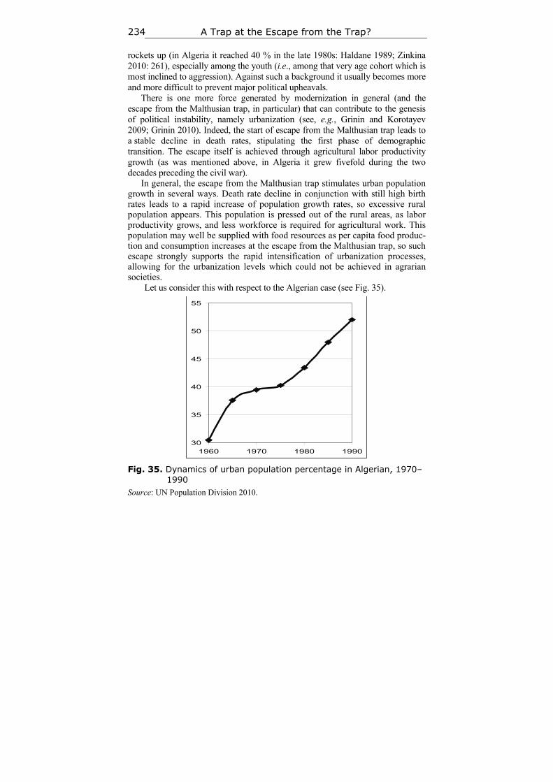
A Trap at the Escape from the Trap? 234
rockets up (in Algeria it reached 40 % in the late 1980s: Haldane 1989; Zinkina 2010: 261), especially among the youth (i.e., among that very age cohort which is most inclined to aggression). Against such a background it usually becomes more and more difficult to prevent major political upheavals.
There is one more force generated by modernization in general (and the escape from the Malthusian trap, in particular) that can contribute to the genesis of political instability, namely urbanization (see, e.g., Grinin and Korotayev 2009; Grinin 2010). Indeed, the start of escape from the Malthusian trap leads to a stable decline in death rates, stipulating the first phase of demographic transition. The escape itself is achieved through agricultural labor productivity growth (as was mentioned above, in Algeria it grew fivefold during the two decades preceding the civil war).
In general, the escape from the Malthusian trap stimulates urban population growth in several ways. Death rate decline in conjunction with still high birth rates leads to a rapid increase of population growth rates, so excessive rural population appears. This population is pressed out of the rural areas, as labor productivity grows, and less workforce is required for agricultural work. This population may well be supplied with food resources as per capita food produc-tion and consumption increases at the escape from the Malthusian trap, so such escape strongly supports the rapid intensification of urbanization processes, allowing for the urbanization levels which could not be achieved in agrarian societies.
Let us consider this with respect to the Algerian case (see Fig. 35).
Fig. 35. Dynamics of urban population percentage in Algerian, 1970–1990
Source: UN Population Division 2010.
30
35
40
45
50
55
1960 1970 1980 1990
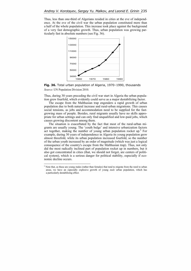
Andrey V. Korotayev, Sergey Yu. Malkov, and Leonid E. Grinin 235
Thus, less than one-third of Algerians resided in cities at the eve of independ-ence. At the eve of the civil war the urban population constituted more than a half of the whole population. This increase took place against the background of a very fast demographic growth. Thus, urban population was growing par-ticularly fast in absolute numbers (see Fig. 36).
Fig. 36. Total urban population of Algeria, 1970–1990, thousands
Source: UN Population Division 2010.
Thus, during 30 years preceding the civil war start in Algeria the urban popula-tion grew fourfold, which evidently could serve as a major destabilizing factor.
The escape from the Malthusian trap engenders a rapid growth of urban population due to both natural increase and rural-urban migrations. This causes social tensions, as jobs and accommodation need to be supplied for the fast-growing mass of people. Besides, rural migrants usually have no skills appro-priate for urban settings and can only find unqualified and low-paid jobs, which causes growing discontent among them.
The situation is exacerbated by the fact that most of the rural-urban mi-grants are usually young. The ‘youth bulge’ and intensive urbanization factors act together, making the number of young urban population rocket up.6 For example, during 30 years of independence in Algeria its young population grew almost threefold, while its urban population increased fourfold, so the number of the urban youth increased by an order of magnitude (which was just a logical consequence of the country's escape from the Malthusian trap). Thus, not only did the most radically inclined part of population rocket up in numbers, but it also got concentrated in cities (that, we should not forget, are centers of politi-cal system), which is a serious danger for political stability, especially if eco-nomic decline occurs. 6 Note that, as these are young males (rather than females) that tend to migrate from the rural to urban
areas, we have an especially explosive growth of young male urban population, which has a particularly destabilizing effect.
3000
5000
7000
9000
11000
13000
15000
1960 1970 1980 1990
A Trap at the Escape from the Trap? 236
It appears quite useful to consider the action of the above-described factors at the ‘grassroots’ level. For this we find it appropriate to reproduce Kepel's description of the events in Algeria that preceded the October riots of 1988, which served as an omen of the forthcoming civil war:
…A population explosion had thrust the children of the fellahs (farmers) into the cities and their outskirts, where conditions were precarious… In 1989, 40 percent of Algeria's population of 24 million were under 15 years of age; the urban population was in excess of 50 percent of the total population… The official unemployment rate was 18.1 percent of the working population, though in reality joblessness was much higher; in 1995 it rose – again officially – to 28 percent. The young urban poor of Algeria were mocked as hittistes – from the Arab word hit, ‘wall’. This jibe derived from the image of jobless young men with nothing to do all day but lean against a wall. The joke was that, in a socialist coun-try where in theory everyone was supposed to have a job, the profession of a hittiste consisted in propping up walls that would otherwise col-lapse. The hittistes were assumed to be passive – unlike the Iranian ones, who were glorified by religious movements and hailed as the messengers of history and the Revelation.
At the time of the October 1988 riots, oil and gas represented 95 percent of the nation's exports and supplied more than 60 percent of the government's yearly budget… The Algerian state was a kind of pop-ular democracy cum oil. The state used its oil revenues to buy social pacification… This balance of power, maintained by subsidies, social-ism, repression, and official ideology, was ultimately dependent on the fragile economic equilibrium created by the high price of oil. In 1986, when oil prices collapsed, half of Algeria's budget was wiped out and the whole structure fell down in ruins. Worse, the population explosion had created a demand for… urban infrastructure, housing, and employment that continued to increase… The construction industry in particular had failed spectacularly to keep pace with the housing demand; the result was the kind of slums and overcrowded urban conditions that invariably lead to social eruption.
It was in this deteriorating climate, punctuated by continual strikes, that riots broke out on October 4, 1988. Mobs of impoverished Algerian youths attacked such symbols of the state as buses, road signs, and Air Algeria agencies, along with any automobile that looked expensive… These days… marked the emergence of the young urban poor as a force to be reckoned with. The once ridiculed hittistes had shown that they could seize and hold power in the streets, shaking to its foundations a re-gime that had excluded them and whose legitimacy they scorned (Kepel 2006: 159–161).
A Trap at the Escape from the Malthusian Trap: Logical and Mathematical Models
Thus, the emergence of major sociopolitical upheavals at the escape from the Malthusian trap is not an abnormal, but a regular phenomenon. So, a special

Andrey V. Korotayev, Sergey Yu. Malkov, and Leonid E. Grinin 237
explanation is rather needed for exceptions, when social systems managed to avoid such shocks.
Why should such upheavals be treated as a regular phenomenon? The an-swer may be summarized as follows:
1) Start of the escape from the Malthusian trap tends to bring about a pre-cipitous death rate decline and, consequently, an explosive acceleration of the population growth rates (which in itself can lead to a certain increase in socio-political tensions).
2) The start of the escape is accompanied by especially strong decreases in infant and under-five mortality, which raises the proportion of the youth in the overall population (and especially in the adult population) – the so-called ‘youth bulge’.
3) This increases sharply the proportion of the part of population most in-clined to radicalism.
4) The impetuous growth of the young population requires the creation of enormous numbers of new jobs, which is a serious economic problem, while the youth unemployment growth can have a particularly strong destabilizing effect, creating an ‘army’ of potential participants for various political upheav-als, including civil wars, revolutions, and state breakdowns.
5) Escape from the Malthusian trap stimulates a vigorous growth of the ur-ban population. Besides, excessive population is pressed out from the country-side by the growth of agricultural labor productivity. Massive rural-urban mi-gration almost inevitably creates a significant number of those dissatisfied with their current position, as initially the rural-urban migrants mostly can only get unskilled low-paid jobs and low-quality accommodation.
6) Escape from the Malthusian trap is achieved through the development of new economic sectors and decline of the old ones. Such structural changes can-not proceed painlessly, as old qualification of workers loses its value and, not having necessary new skills, these workers are obliged to take up low-qualified jobs, which makes them socially discontent.
7) The young people make up the majority of rural-urban migrants, so the ‘youth bulge’ and intensive urbanization factors act together, producing a par-ticularly strong destabilizing effect. Not only does the most radically inclined part of population rocket up in numbers, but it also gets concentrated in major cities / political centers.
8) This can result in serious political destabilization even against the back-ground of a rather stable economic growth (see Fig. 37). The probability of political destabilization naturally increases dramatically if an economic crisis occurs, or if the government loses its legitimacy due to any other causes (such as military defeats), though the recent ‘Arab Spring’ events have demonstrated once again in a rather salient way that even this is not really necessary (see, e.g., Korotayev and Zinkina 2011).
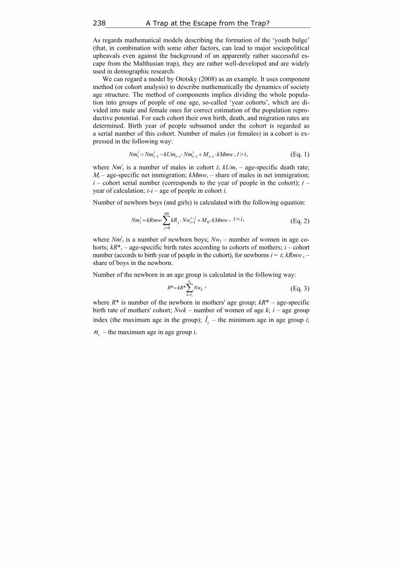
A Trap at the Escape from the Trap? 238
As regards mathematical models describing the formation of the ‘youth bulge’ (that, in combination with some other factors, can lead to major sociopolitical upheavals even against the background of an apparently rather successful es-cape from the Malthusian trap), they are rather well-developed and are widely used in demographic research.
We can regard a model by Ototsky (2008) as an example. It uses component method (or cohort analysis) to describe mathematically the dynamics of society age structure. The method of components implies dividing the whole popula-tion into groups of people of one age, so-called ‘year cohorts’, which are di-vided into male and female ones for correct estimation of the population repro-ductive potential. For each cohort their own birth, death, and migration rates are determined. Birth year of people subsumed under the cohort is regarded as a serial number of this cohort. Number of males (or females) in a cohort is ex-pressed in the following way:
kMmwMNmkUmNmNm ititit
it
it 11 , ,it (Eq. 1)
where Nmit is a number of males in cohort i; kUmt – age-specific death rate;
Mt – age-specific net immigration; kMmwt – share of males in net immigration; i – cohort serial number (corresponds to the year of people in the cohort); t – year of calculation; t-i – age of people in cohort i.
Number of newborn boys (and girls) is calculated with the following equation:
kMmwMNwkRkRmwNmj
jttj
it
0
60
01
, ,it (Eq. 2)
where Nmit is a number of newborn boys; Nwt – number of women in age co-
horts; kR*t – age-specific birth rates according to cohorts of mothers; i – cohort number (accords to birth year of people in the cohort), for newborns i = t; kRmw t – share of boys in the newborn.
Number of the newborn in an age group is calculated in the following way:
i
i
n
lkkNwkRR ** , (Eq. 3)
where R* is number of the newborn in mothers' age group; kR* – age-specific birth rate of mothers' cohort; Nwk – number of women of age k; i – age group
index (the maximum age in the group); il – the minimum age in age group i;
in – the maximum age in age group i.
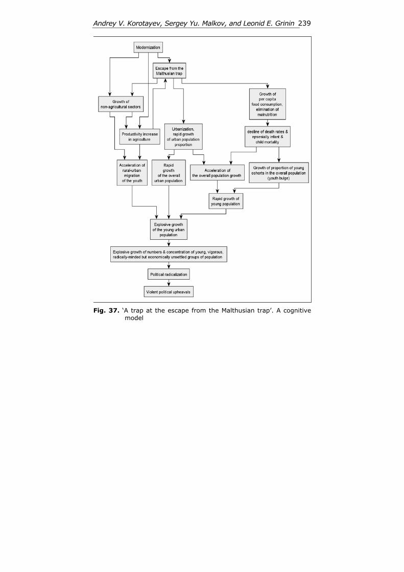
Andrey V. Korotayev, Sergey Yu. Malkov, and Leonid E. Grinin 239
Fig. 37. ‘A trap at the escape from the Malthusian trap’. A cognitive
model
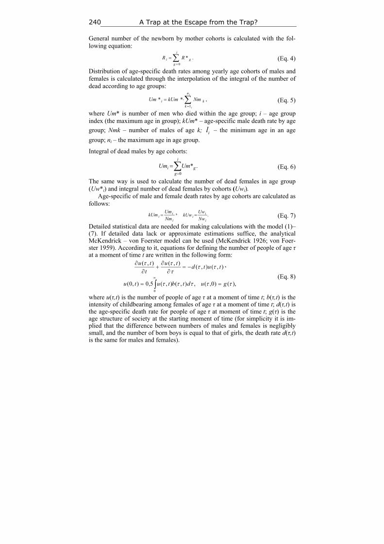
A Trap at the Escape from the Trap? 240
General number of the newborn by mother cohorts is calculated with the fol-lowing equation:
.*0
i
ggi RR
(Eq. 4)
Distribution of age-specific death rates among yearly age cohorts of males and females is calculated through the interpolation of the integral of the number of dead according to age groups:
,**1
i
i
n
kki NmkUmUm (Eq. 5)
where Um* is number of men who died within the age group; i – age group index (the maximum age in group); kUm* – age-specific male death rate by age
group; Nmk – number of males of age k; il – the minimum age in an age
group; ni – the maximum age in age group.
Integral of dead males by age cohorts:
.*0
i
ggi UmUm (Eq. 6)
The same way is used to calculate the number of dead females in age group (Uw*i) and integral number of dead females by cohorts (Uwi).
Age-specific of male and female death rates by age cohorts are calculated as follows:
i
ii Nm
UmkUm , .
i
ii Nw
UwkUw (Eq. 7)
Detailed statistical data are needed for making calculations with the model (1)–(7). If detailed data lack or approximate estimations suffice, the analytical McKendrick – von Foerster model can be used (McKendrick 1926; von Foer-ster 1959). According to it, equations for defining the number of people of age τ at a moment of time t are written in the following form:
),(),(),(),(
tutdtu
t
tu
,
),()0,(,),(),(5,0),0(0
gudtbtutu
(Eq. 8)
where u(τ,t) is the number of people of age τ at a moment of time t; b(τ,t) is the intensity of childbearing among females of age τ at a moment of time t; d(τ,t) is the age-specific death rate for people of age τ at moment of time t; g(τ) is the age structure of society at the starting moment of time (for simplicity it is im-plied that the difference between numbers of males and females is negligibly small, and the number of born boys is equal to that of girls, the death rate d(τ,t) is the same for males and females).
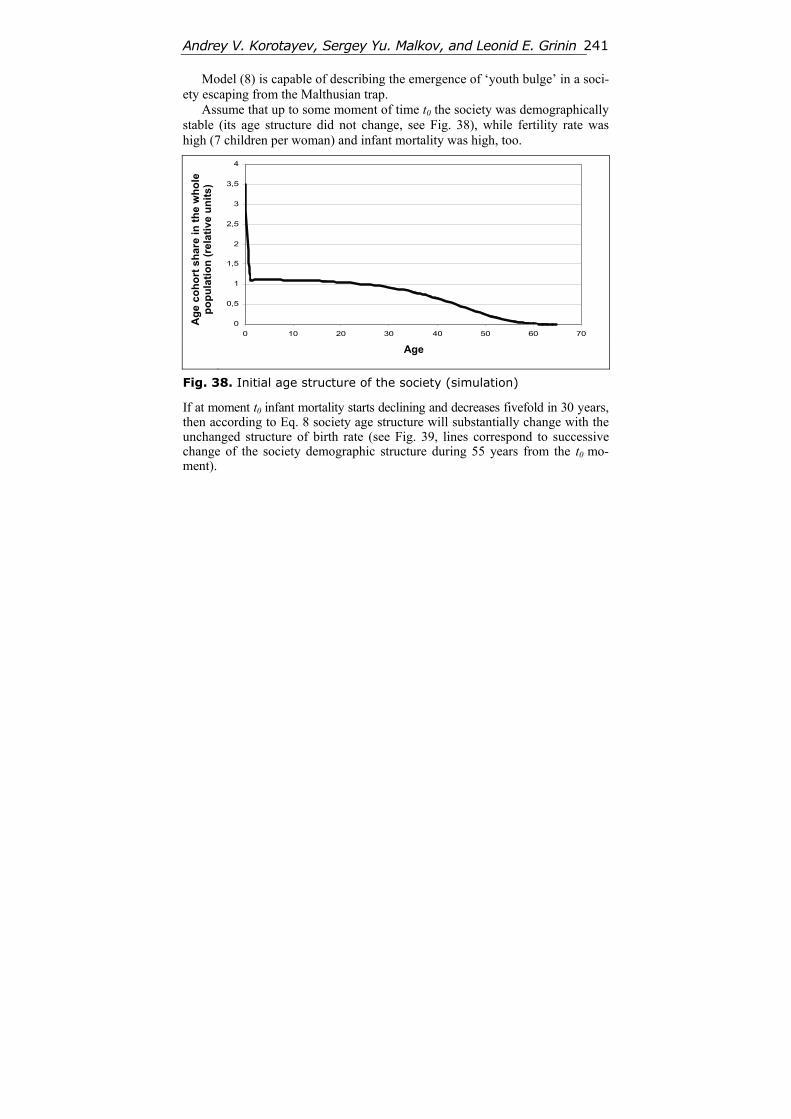
Andrey V. Korotayev, Sergey Yu. Malkov, and Leonid E. Grinin 241
Model (8) is capable of describing the emergence of ‘youth bulge’ in a soci-ety escaping from the Malthusian trap.
Assume that up to some moment of time t0 the society was demographically stable (its age structure did not change, see Fig. 38), while fertility rate was high (7 children per woman) and infant mortality was high, too.
Ag
e c
oh
ort
sh
are
in t
he
wh
ole
p
op
ula
tio
n (
rela
tive
un
its
)
0
0,5
1
1,5
2
2,5
3
3,5
4
0 10 20 30 40 50 60 70
Age
Fig. 38. Initial age structure of the society (simulation)
If at moment t0 infant mortality starts declining and decreases fivefold in 30 years, then according to Eq. 8 society age structure will substantially change with the unchanged structure of birth rate (see Fig. 39, lines correspond to successive change of the society demographic structure during 55 years from the t0 mo-ment).
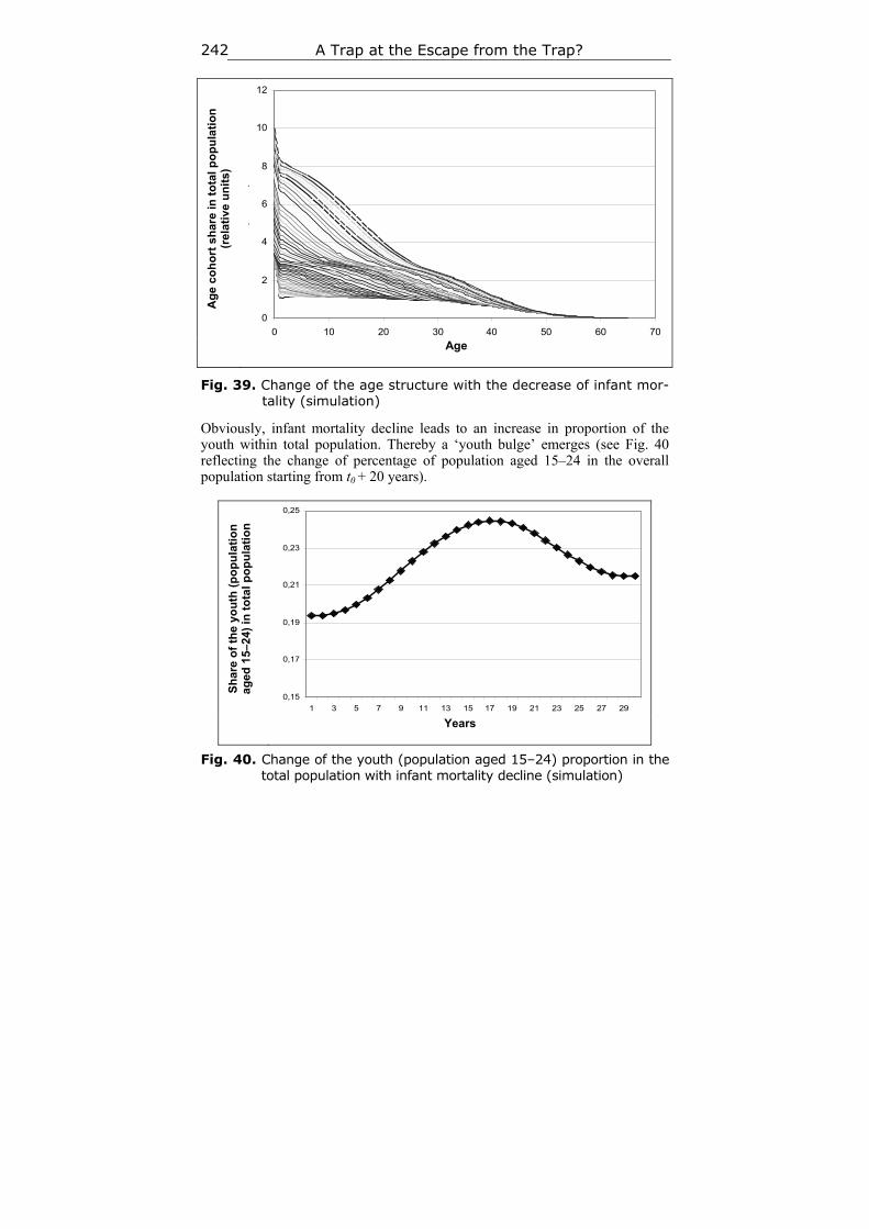
A Trap at the Escape from the Trap? 242
Ag
e c
oh
ort
sh
are
in t
ota
l p
op
ula
tio
n
(rel
ativ
e u
nit
s)
0
2
4
6
8
10
12
0 10 20 30 40 50 60 70
()
Age
Fig. 39. Change of the age structure with the decrease of infant mor-tality (simulation)
Obviously, infant mortality decline leads to an increase in proportion of the youth within total population. Thereby a ‘youth bulge’ emerges (see Fig. 40 reflecting the change of percentage of population aged 15–24 in the overall population starting from t0 + 20 years).
Sh
are
of
the
yo
uth
(p
op
ula
tio
n
aged
15–
24)
in t
ota
l p
op
ula
tio
n
0,15
0,17
0,19
0,21
0,23
0,25
1 3 5 7 9 11 13 15 17 19 21 23 25 27 29
Years
Fig. 40. Change of the youth (population aged 15–24) proportion in the total population with infant mortality decline (simulation)
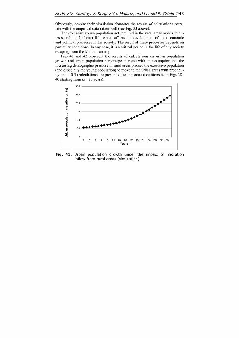
Andrey V. Korotayev, Sergey Yu. Malkov, and Leonid E. Grinin 243
Obviously, despite their simulation character the results of calculations corre-late with the empirical data rather well (see Fig. 33 above).
The excessive young population not required in the rural areas moves to cit-ies searching for better life, which affects the development of socioeconomic and political processes in the society. The result of these processes depends on particular conditions. In any case, it is a critical period in the life of any society escaping from the Malthusian trap.
Figs 41 and 42 represent the results of calculations on urban population growth and urban population percentage increase with an assumption that the increasing demographic pressure in rural areas presses the excessive population (and especially the young population) to move to the urban areas with probabil-ity about 0.5 (calculations are presented for the same conditions as in Figs 38–40 starting from t0 + 20 years).
Urb
an p
op
ula
tio
n (
rela
tive
un
its
)
0
50
100
150
200
250
300
1 3 5 7 9 11 13 15 17 19 21 23 25 27 29
Years
Fig. 41. Urban population growth under the impact of migration inflow from rural areas (simulation)
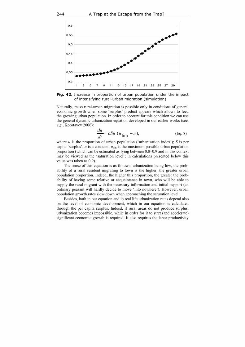
A Trap at the Escape from the Trap? 244
Fig. 42. Increase in proportion of urban population under the impact of intensifying rural-urban migration (simulation)
Naturally, mass rural-urban migration is possible only in conditions of general economic growth when some ‘surplus’ product appears which allows to feed the growing urban population. In order to account for this condition we can use the general dynamic urbanization equation developed in our earlier works (see, e.g., Korotayev 2006):
),lim( uuaSudt
du (Eq. 8)
where u is the proportion of urban population (‘urbanization index’); S is per capita ‘surplus’; а is a constant; ulim is the maximum possible urban population proportion (which can be estimated as lying between 0.8–0.9 and in this context may be viewed as the ‘saturation level’; in calculations presented below this value was taken as 0.9).
The sense of this equation is as follows: urbanization being low, the prob-ability of a rural resident migrating to town is the higher, the greater urban population proportion. Indeed, the higher this proportion, the greater the prob-ability of having some relative or acquaintance in town, who will be able to supply the rural migrant with the necessary information and initial support (an ordinary peasant will hardly decide to move ‘into nowhere’). However, urban population growth rates slow down when approaching the saturation level.
Besides, both in our equation and in real life urbanization rates depend also on the level of economic development, which in our equation is calculated through the per capita surplus. Indeed, if rural areas do not produce surplus, urbanization becomes impossible, while in order for it to start (and accelerate) significant economic growth is required. It also requires the labor productivity
0,3
0,35
0,4
0,45
0,5
0,55
0,6
1 3 5 7 9 11 13 15 17 19 21 23 25 27 29
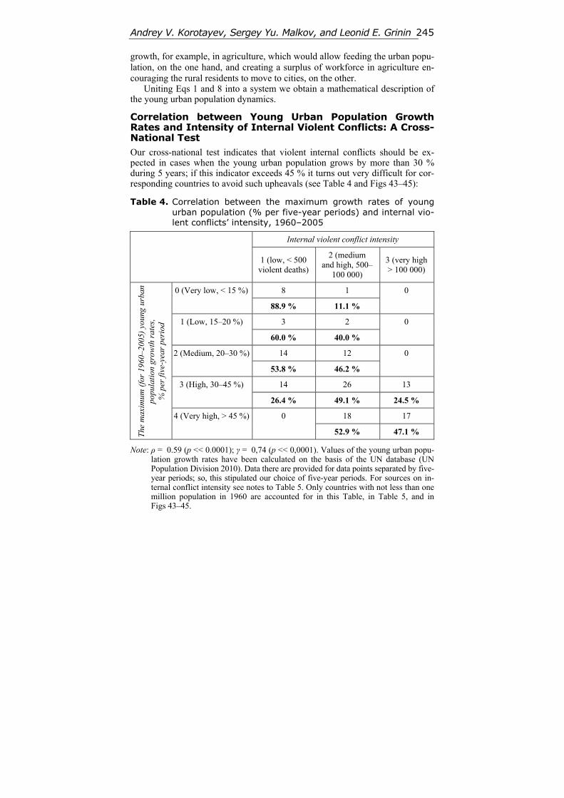
Andrey V. Korotayev, Sergey Yu. Malkov, and Leonid E. Grinin 245
growth, for example, in agriculture, which would allow feeding the urban popu-lation, on the one hand, and creating a surplus of workforce in agriculture en-couraging the rural residents to move to cities, on the other.
Uniting Eqs 1 and 8 into a system we obtain a mathematical description of the young urban population dynamics.
Correlation between Young Urban Population Growth Rates and Intensity of Internal Violent Conflicts: A Cross-National Test Our cross-national test indicates that violent internal conflicts should be ex-pected in cases when the young urban population grows by more than 30 % during 5 years; if this indicator exceeds 45 % it turns out very difficult for cor-responding countries to avoid such upheavals (see Table 4 and Figs 43–45):
Table 4. Correlation between the maximum growth rates of young urban population (% per five-year periods) and internal vio-lent conflicts’ intensity, 1960–2005
Internal violent conflict intensity
1 (low, < 500 violent deaths)
2 (medium and high, 500–
100 000)
3 (very high > 100 000)
8 1 0 (Very low, < 15 %)
88.9 % 11.1 %
0
3 2 1 (Low, 15–20 %)
60.0 % 40.0 %
0
14 12 2 (Medium, 20–30 %)
53.8 % 46.2 %
0
14 26 13 3 (High, 30–45 %)
26.4 % 49.1 % 24.5 %
18 17
The
max
imum
(fo
r 19
60–2
005)
you
ng u
rban
po
pula
tion
gro
wth
rat
es,
% p
er fi
ve-y
ear
peri
od
4 (Very high, > 45 %) 0
52.9 % 47.1 %
Note: ρ = 0.59 (p << 0.0001); γ = 0,74 (p << 0,0001). Values of the young urban popu-lation growth rates have been calculated on the basis of the UN database (UN Population Division 2010). Data there are provided for data points separated by five-year periods; so, this stipulated our choice of five-year periods. For sources on in-ternal conflict intensity see notes to Table 5. Only countries with not less than one million population in 1960 are accounted for in this Table, in Table 5, and in Figs 43–45.
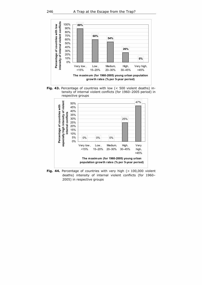
A Trap at the Escape from the Trap? 246
89%
60%54%
26%
0%0%
10%20%30%40%50%60%70%80%90%
100%
Very low ,<15%
Low ,15–20%
Medium,20–30%
High,30–45%
Very high,>45%
The maximum (for 1960-2005) young urban population growth rates (% per 5-year period)
Per
cen
tag
e o
f co
un
trie
s w
ith
low
in
ten
sity
of
inte
rnal
vio
len
t co
nfl
icts
Fig. 43. Percentage of countries with low (< 500 violent deaths) in-
tensity of internal violent conflicts (for 1960–2005 period) in respective groups
0% 0% 0%
25%
47%
0%5%
10%15%20%25%30%35%40%45%50%
Very low ,<15%
Low ,15–20%
Medium,20–30%
High,30–45%
Veryhigh,>45%
The maximum (for 1960-2005) young urban population growth rates (% per 5-year period)
Per
cen
tag
e o
f co
un
trie
s w
ith
es
pec
ially
hig
h in
ten
sity
of
vio
len
t in
tern
al c
on
flic
ts
Fig. 44. Percentage of countries with very high (> 100,000 violent
deaths) intensity of internal violent conflicts (for 1960–2005) in respective groups
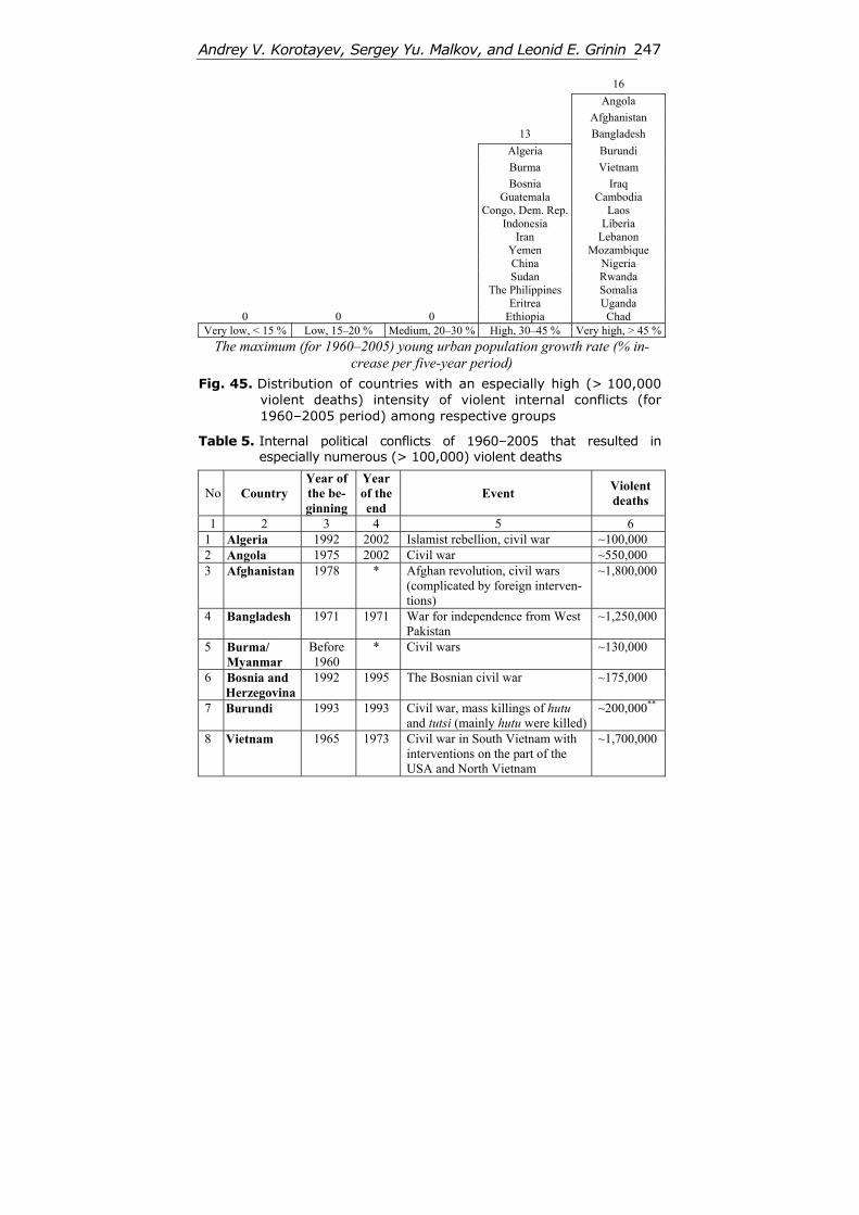
Andrey V. Korotayev, Sergey Yu. Malkov, and Leonid E. Grinin 247
16
Angola
Afghanistan
13 Bangladesh
Algeria Burundi
Burma Vietnam
Bosnia Iraq Guatemala Cambodia Congo, Dem. Rep. Laos Indonesia Liberia Iran Lebanon
Yemen Mozambique China Nigeria Sudan Rwanda The Philippines Somalia Eritrea Uganda
0 0 0 Ethiopia Chad Very low, < 15 % Low, 15–20 % Medium, 20–30 % High, 30–45 % Very high, > 45 %
The maximum (for 1960–2005) young urban population growth rate (% in-crease per five-year period)
Fig. 45. Distribution of countries with an especially high (> 100,000 violent deaths) intensity of violent internal conflicts (for 1960–2005 period) among respective groups
Table 5. Internal political conflicts of 1960–2005 that resulted in especially numerous (> 100,000) violent deaths
No Country Year of the be-ginning
Year of the end
Event Violent deaths
1 2 3 4 5 6 1 Algeria 1992 2002 Islamist rebellion, civil war ~100,000 2 Angola 1975 2002 Civil war ~550,000 3 Afghanistan 1978 * Afghan revolution, civil wars
(complicated by foreign interven-tions)
~1,800,000
4 Bangladesh 1971 1971 War for independence from West Pakistan
~1,250,000
5 Burma/ Myanmar
Before 1960
* Civil wars ~130,000
6 Bosnia and Herzegovina
1992 1995 The Bosnian civil war ~175,000
7 Burundi 1993 1993 Civil war, mass killings of hutu and tutsi (mainly hutu were killed)
~200,000**
8 Vietnam 1965 1973 Civil war in South Vietnam with interventions on the part of the USA and North Vietnam
~1,700,000

A Trap at the Escape from the Trap? 248
1 2 3 4 5 6 9 Guatemala 1960 1996 Civil war ~200,000
1960 1965 Congolese crisis ~100,000 10 Congo, Dem. Rep. (Zaire)
1998 2009 Civil wars ~3,800,000
11 Indonesia 1965 1966 Coup attempt, mass executions ~400,000 12 Iraq 1961 * Kurd upsurges in the north, Shia
insurrections in the south, political upheavals of the 2000s
~100,000
13 Iran 1978 1979 Islamic revolution ~100,000 14 Yemen 1962 1970 Revolution and civil war ~100,000 15 Cambodia 1970 1991 Civil wars and their consequences
(complicated by foreign interven-tions)
~2,500,000
16 China 1966 1969 ‘Cultural revolution’ From 2,000,000 to 7,000,000
17 Laos 1960 1973 Civil war within the Second Indo-china War
From 70,000 to 250,000
18 Liberia 1989 1997 Civil wars ~150,000 19 Lebanon 1975 1990 Civil war complicated by numer-
ous cases of foreign intervention ~150,000
20 Mozam-bique
1975 1992 Civil war ~1,000,000
21 Nigeria 1966 1970 Coup, civil war of Biafra From 600,000 to 1,000,000
22 Rwanda 1994 1994 Civil war, mass killings of the Tutsi
~937,000 **
23 Somalia 1991 * Civil war, state breakdown, chaos, anarchy
~400,000**
1955 1972 Civil war ~500,000 1983 * Civil war ~1,900,000
24 Sudan
2003 * Darfur conflict From 70,000 to more than 180,000
25 Uganda 1979 1986 Civil wars ~300,000**
26 The Philip-pines
Since 1972
* War against guerillas From 50,000 to 150,000
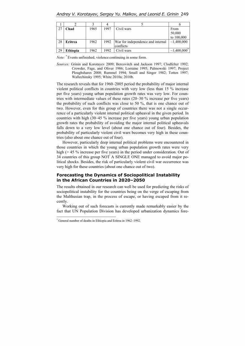
Andrey V. Korotayev, Sergey Yu. Malkov, and Leonid E. Grinin 249
1 2 3 4 5 6 27 Chad 1965 1997 Civil wars From
50,000 to 100,000
28 Eritrea 1962 1992 War for independence and internal conflicts
~1,400,000
29 Ethiopia 1962 1992 Civil wars ~1,400,0007
Note: * Events unfinished, violence continuing in some form.
Sources: Grinin and Korotayev 2009; Bercovitch and Jackson 1997; Clodfelter 1992; Crowder, Fage, and Oliver 1986; Lorraine 1995; Palmowski 1997; Project Ploughshares 2008; Rummel 1994; Small and Singer 1982; Totten 1997; Wallechinsky 1995; White 2010a; 2010b.
The research reveals that for 1960–2005 period the probability of major internal violent political conflicts in countries with very low (less than 15 % increase per five years) young urban population growth rates was very low. For coun-tries with intermediate values of these rates (20–30 % increase per five years) the probability of such conflicts was close to 50 %, that is one chance out of two. However, even for this group of countries there was not a single occur-rence of a particularly violent internal political upheaval in the given period. In countries with high (30–45 % increase per five years) young urban population growth rates the probability of avoiding the major internal political upheavals falls down to a very low level (about one chance out of four). Besides, the probability of particularly violent civil wars becomes very high in these coun-tries (also about one chance out of four).
However, particularly deep internal political problems were encountered in those countries in which the young urban population growth rates were very high (> 45 % increase per five years) in the period under consideration. Out of 34 countries of this group NOT A SINGLE ONE managed to avoid major po-litical shocks. Besides, the risk of particularly violent civil war occurrence was very high for these countries (about one chance out of two).
Forecasting the Dynamics of Sociopolitical Instability in the African Countries in 2020–2050
The results obtained in our research can well be used for predicting the risks of sociopolitical instability for the countries being on the verge of escaping from the Malthusian trap, in the process of escape, or having escaped from it re-cently.
Working out of such forecasts is currently made remarkably easier by the fact that UN Population Division has developed urbanization dynamics fore- 7 General number of deaths in Ethiopia and Eritrea in 1962–1992.
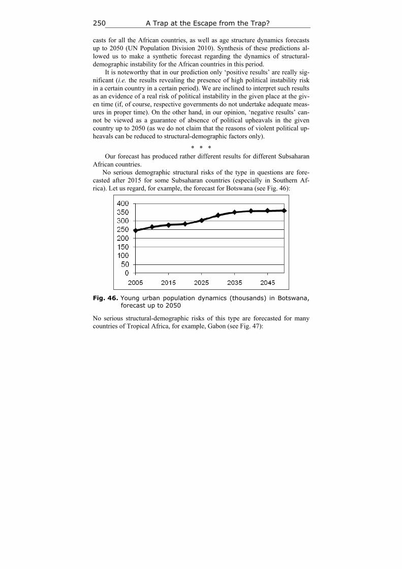
A Trap at the Escape from the Trap? 250
casts for all the African countries, as well as age structure dynamics forecasts up to 2050 (UN Population Division 2010). Synthesis of these predictions al-lowed us to make a synthetic forecast regarding the dynamics of structural-demographic instability for the African countries in this period.
It is noteworthy that in our prediction only ‘positive results’ are really sig-nificant (i.e. the results revealing the presence of high political instability risk in a certain country in a certain period). We are inclined to interpret such results as an evidence of a real risk of political instability in the given place at the giv-en time (if, of course, respective governments do not undertake adequate meas-ures in proper time). On the other hand, in our opinion, ‘negative results’ can-not be viewed as a guarantee of absence of political upheavals in the given country up to 2050 (as we do not claim that the reasons of violent political up-heavals can be reduced to structural-demographic factors only).
* * * Our forecast has produced rather different results for different Subsaharan
African countries. No serious demographic structural risks of the type in questions are fore-
casted after 2015 for some Subsaharan countries (especially in Southern Af-rica). Let us regard, for example, the forecast for Botswana (see Fig. 46):
Fig. 46. Young urban population dynamics (thousands) in Botswana, forecast up to 2050
No serious structural-demographic risks of this type are forecasted for many countries of Tropical Africa, for example, Gabon (see Fig. 47):
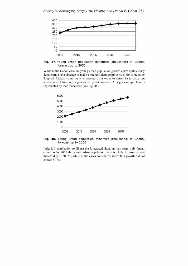
Andrey V. Korotayev, Sergey Yu. Malkov, and Leonid E. Grinin 251
Fig. 47. Young urban population dynamics (thousands) in Gabon,
forecast up to 2050
While in the Gabon case the young urban population growth curve quite clearly demonstrates the absence of major structural-demographic risks, for some other Tropical African countries it is necessary (in order to detect it) to carry out an analysis of time series generated by our forecast. A bright example here is represented by the Ghana case (see Fig. 48).
Fig. 48. Young urban population dynamics (thousands) in Ghana,
forecast up to 2050
Indeed, in application to Ghana the forecasted situation may seem truly threat-ening, as by 2050 the young urban population there is likely to grow almost threefold (i.e., 200 %; while in the cases considered above this growth did not exceed 50 %).
0
1000
2000
3000
4000
5000
6000
2005 2015 2025 2035 2045
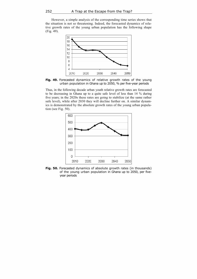
A Trap at the Escape from the Trap? 252
However, a simple analysis of the corresponding time series shows that the situation is not so threatening. Indeed, the forecasted dynamics of rela-tive growth rates of the young urban population has the following shape (Fig. 49).
Fig. 49. Forecasted dynamics of relative growth rates of the young urban population in Ghana up to 2050, % per five-year periods
Thus, in the following decade urban youth relative growth rates are forecasted to be decreasing in Ghana up to a quite safe level of less than 14 % during five years; in the 2020s these rates are going to stabilize (at the same rather safe level), while after 2030 they will decline further on. A similar dynam-ics is demonstrated by the absolute growth rates of the young urban popula-tion (see Fig. 50).
Fig. 50. Forecasted dynamics of absolute growth rates (in thousands) of the young urban population in Ghana up to 2050, per five-year periods
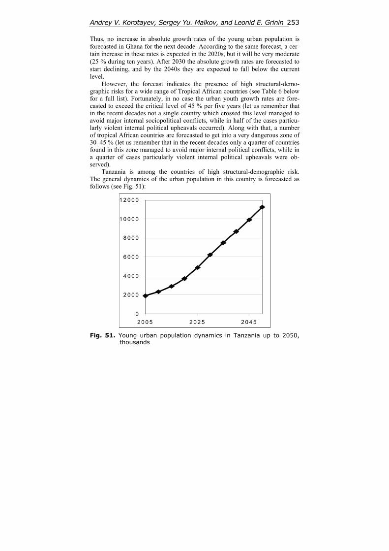
Andrey V. Korotayev, Sergey Yu. Malkov, and Leonid E. Grinin 253
Thus, no increase in absolute growth rates of the young urban population is forecasted in Ghana for the next decade. According to the same forecast, a cer-tain increase in these rates is expected in the 2020s, but it will be very moderate (25 % during ten years). After 2030 the absolute growth rates are forecasted to start declining, and by the 2040s they are expected to fall below the current level.
However, the forecast indicates the presence of high structural-demo-graphic risks for a wide range of Tropical African countries (see Table 6 below for a full list). Fortunately, in no case the urban youth growth rates are fore-casted to exceed the critical level of 45 % per five years (let us remember that in the recent decades not a single country which crossed this level managed to avoid major internal sociopolitical conflicts, while in half of the cases particu-larly violent internal political upheavals occurred). Along with that, a number of tropical African countries are forecasted to get into a very dangerous zone of 30–45 % (let us remember that in the recent decades only a quarter of countries found in this zone managed to avoid major internal political conflicts, while in a quarter of cases particularly violent internal political upheavals were ob-served).
Tanzania is among the countries of high structural-demographic risk. The general dynamics of the urban population in this country is forecasted as follows (see Fig. 51):
Fig. 51. Young urban population dynamics in Tanzania up to 2050, thousands
0
2 0 0 0
4 0 0 0
6 0 0 0
8 0 0 0
1 0 0 0 0
1 2 0 0 0
2 0 0 5 2 0 2 5 2 0 4 5
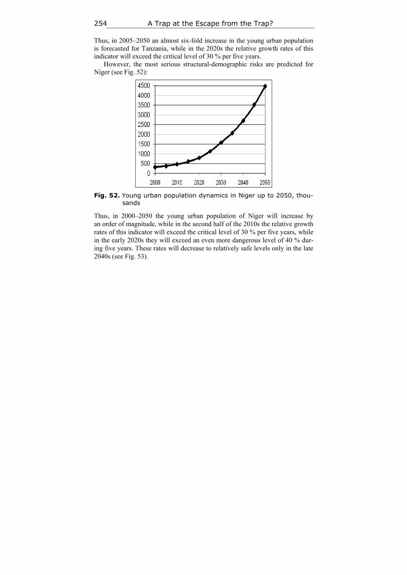
A Trap at the Escape from the Trap? 254
Thus, in 2005–2050 an almost six-fold increase in the young urban population is forecasted for Tanzania, while in the 2020s the relative growth rates of this indicator will exceed the critical level of 30 % per five years.
However, the most serious structural-demographic risks are predicted for Niger (see Fig. 52):
Fig. 52. Young urban population dynamics in Niger up to 2050, thou-sands
Thus, in 2000–2050 the young urban population of Niger will increase by an order of magnitude, while in the second half of the 2010s the relative growth rates of this indicator will exceed the critical level of 30 % per five years, while in the early 2020s they will exceed an even more dangerous level of 40 % dur-ing five years. These rates will decrease to relatively safe levels only in the late 2040s (see Fig. 53).
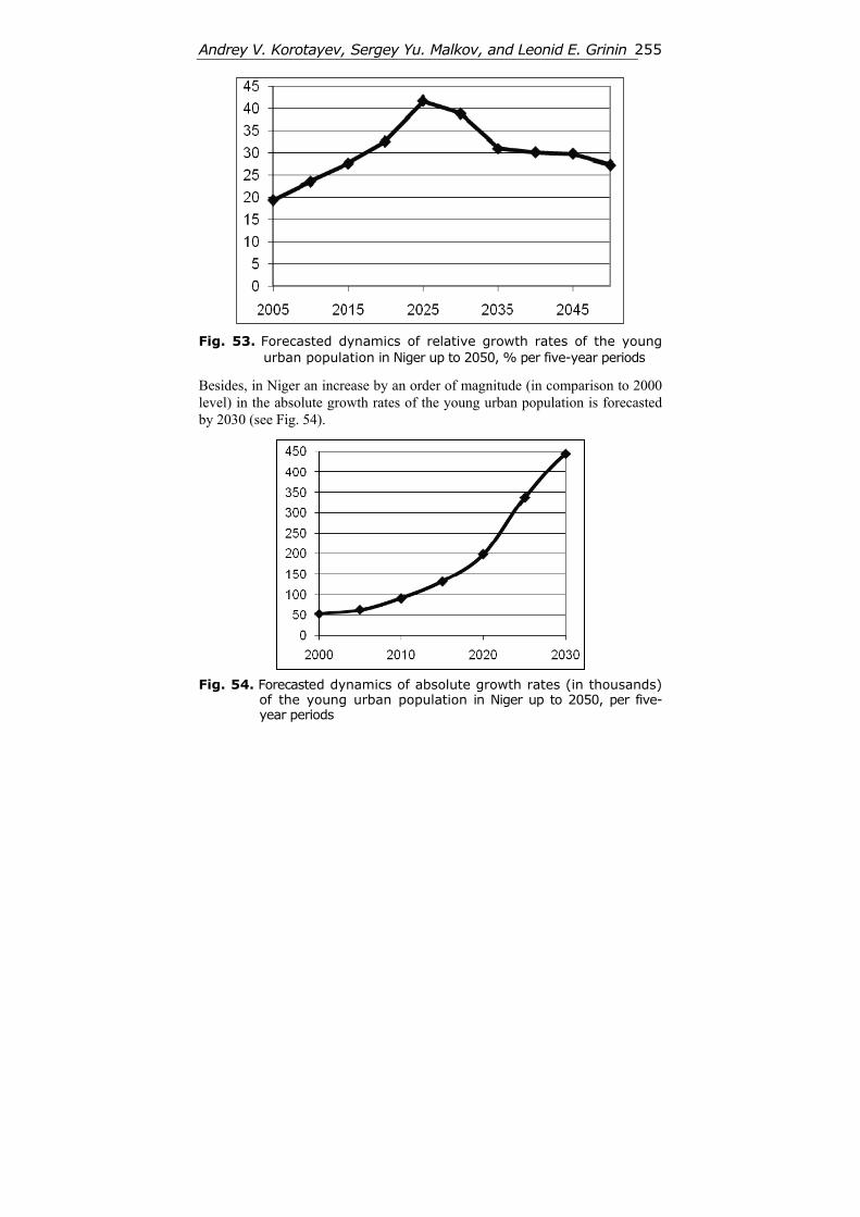
Andrey V. Korotayev, Sergey Yu. Malkov, and Leonid E. Grinin 255
Fig. 53. Forecasted dynamics of relative growth rates of the young
urban population in Niger up to 2050, % per five-year periods
Besides, in Niger an increase by an order of magnitude (in comparison to 2000 level) in the absolute growth rates of the young urban population is forecasted by 2030 (see Fig. 54).
Fig. 54. Forecasted dynamics of absolute growth rates (in thousands)
of the young urban population in Niger up to 2050, per five-year periods
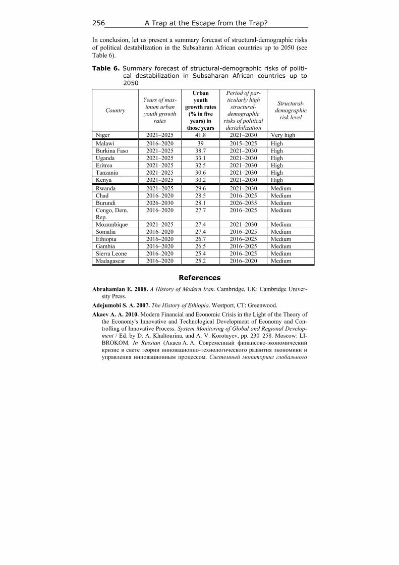
A Trap at the Escape from the Trap? 256
In conclusion, let us present a summary forecast of structural-demographic risks of political destabilization in the Subsaharan African countries up to 2050 (see Table 6).
Table 6. Summary forecast of structural-demographic risks of politi-cal destabilization in Subsaharan African countries up to 2050
Country
Years of max-imum urban youth growth
rates
Urban youth
growth rates (% in five years) in
those years
Period of par-ticularly high
structural-demographic
risks of political destabilization
Structural-demographic
risk level
Niger 2021–2025 41.8 2021–2030 Very high
Malawi 2016–2020 39 2015–2025 High Burkina Faso 2021–2025 38.7 2021–2030 High Uganda 2021–2025 33.1 2021–2030 High Eritrea 2021–2025 32.5 2021–2030 High Tanzania 2021–2025 30.6 2021–2030 High Kenya 2021–2025 30.2 2021–2030 High
Rwanda 2021–2025 29.6 2021–2030 Medium Chad 2016–2020 28.5 2016–2025 Medium Burundi 2026–2030 28.1 2026–2035 Medium Congo, Dem. Rep.
2016–2020 27.7 2016–2025 Medium
Mozambique 2021–2025 27.4 2021–2030 Medium Somalia 2016–2020 27.4 2016–2025 Medium Ethiopia 2016–2020 26.7 2016–2025 Medium Gambia 2016–2020 26.5 2016–2025 Medium Sierra Leone 2016–2020 25.4 2016–2025 Medium Madagascar 2016–2020 25.2 2016–2020 Medium
References
Abrahamian E. 2008. A History of Modern Iran. Cambridge, UK: Cambridge Univer-sity Press.
Adejumobi S. A. 2007. The History of Ethiopia. Westport, CT: Greenwood.
Akaev A. A. 2010. Modern Financial and Economic Crisis in the Light of the Theory of the Economy's Innovative and Technological Development of Economy and Con-trolling of Innovative Process. System Monitoring of Global and Regional Develop-ment / Ed. by D. A. Khaltourina, and A. V. Korotayev, pp. 230–258. Moscow: LI-BROKOM. In Russian (Акаев А. А. Современный финансово-экономический кризис в свете теории инновационно-технологического развития экономики и управления инновационным процессом. Системный мониторинг глобального
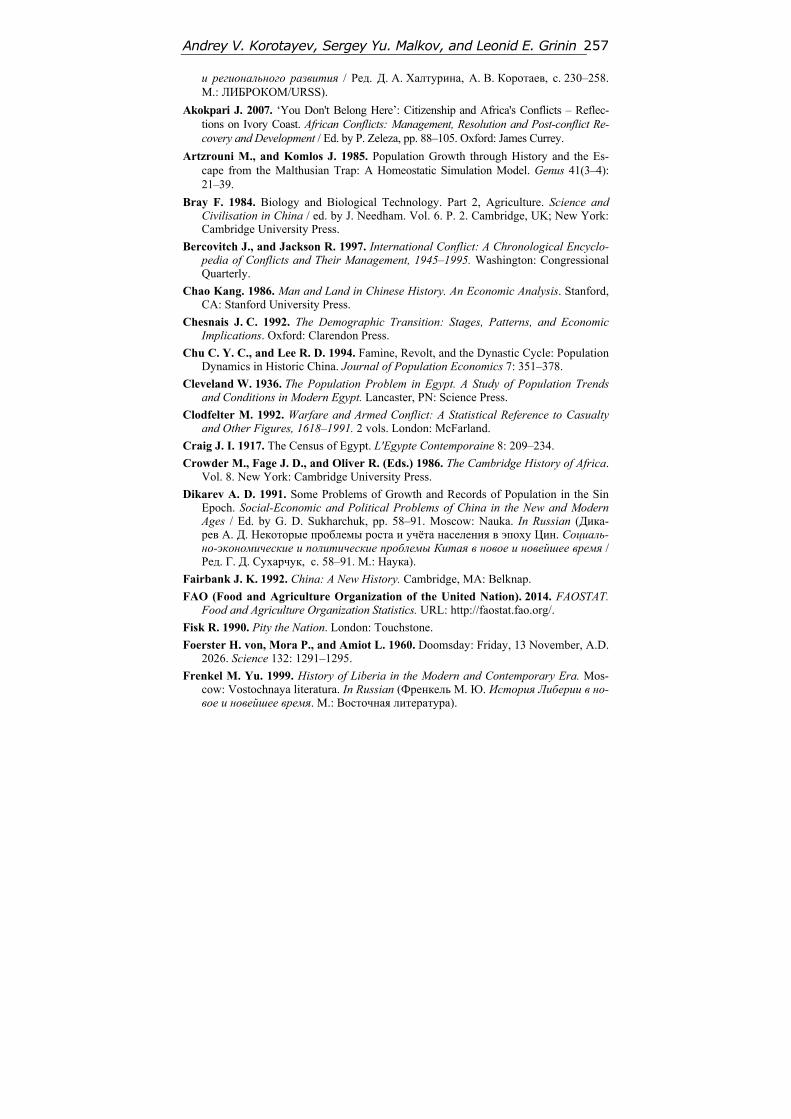
Andrey V. Korotayev, Sergey Yu. Malkov, and Leonid E. Grinin 257
и регионального развития / Ред. Д. А. Халтурина, А. В. Коротаев, с. 230–258. М.: ЛИБРОКОМ/URSS).
Akokpari J. 2007. ‘You Don't Belong Here’: Citizenship and Africa's Conflicts – Reflec-tions on Ivory Coast. African Conflicts: Management, Resolution and Post-conflict Re-covery and Development / Ed. by P. Zeleza, pp. 88–105. Oxford: James Currey.
Artzrouni M., and Komlos J. 1985. Population Growth through History and the Es-cape from the Malthusian Trap: A Homeostatic Simulation Model. Genus 41(3–4): 21–39.
Bray F. 1984. Biology and Biological Technology. Part 2, Agriculture. Science and Civilisation in China / ed. by J. Needham. Vol. 6. P. 2. Cambridge, UK; New York: Cambridge University Press.
Bercovitch J., and Jackson R. 1997. International Conflict: A Chronological Encyclo-pedia of Conflicts and Their Management, 1945–1995. Washington: Congressional Quarterly.
Chao Kang. 1986. Man and Land in Chinese History. An Economic Analysis. Stanford, CA: Stanford University Press.
Chesnais J. C. 1992. The Demographic Transition: Stages, Patterns, and Economic Implications. Oxford: Clarendon Press.
Chu C. Y. C., and Lee R. D. 1994. Famine, Revolt, and the Dynastic Cycle: Population Dynamics in Historic China. Journal of Population Economics 7: 351–378.
Cleveland W. 1936. The Population Problem in Egypt. A Study of Population Trends and Conditions in Modern Egypt. Lancaster, PN: Science Press.
Clodfelter M. 1992. Warfare and Armed Conflict: A Statistical Reference to Casualty and Other Figures, 1618–1991. 2 vols. London: McFarland.
Craig J. I. 1917. The Census of Egypt. L'Egypte Contemporaine 8: 209–234.
Crowder M., Fage J. D., and Oliver R. (Eds.) 1986. The Cambridge History of Africa. Vol. 8. New York: Cambridge University Press.
Dikarev A. D. 1991. Some Problems of Growth and Records of Population in the Sin Epoch. Social-Economic and Political Problems of China in the New and Modern Ages / Ed. by G. D. Sukharchuk, pp. 58–91. Moscow: Nauka. In Russian (Дика- рев А. Д. Некоторые проблемы роста и учёта населения в эпоху Цин. Социаль-но-экономические и политические проблемы Китая в новое и новейшее время / Ред. Г. Д. Сухарчук, с. 58–91. М.: Наука).
Fairbank J. K. 1992. China: A New History. Cambridge, MA: Belknap.
FAO (Food and Agriculture Organization of the United Nation). 2014. FAOSTAT. Food and Agriculture Organization Statistics. URL: http://faostat.fao.org/.
Fisk R. 1990. Pity the Nation. London: Touchstone.
Foerster H. von, Mora P., and Amiot L. 1960. Doomsday: Friday, 13 November, A.D. 2026. Science 132: 1291–1295.
Frenkel M. Yu. 1999. History of Liberia in the Modern and Contemporary Era. Mos-cow: Vostochnaya literatura. In Russian (Френкель М. Ю. История Либерии в но-вое и новейшее время. М.: Восточная литература).
A Trap at the Escape from the Trap? 258
Friedman T. 1998. From Beirut to Jerusalem. London: HarperCollins.
Fuller G. E. 2004. The Youth Crisis in Middle Eastern Society. Clinton Township, MI: Institute for Social Policy and Understanding.
Goldstone J. 1991. Revolution and Rebellion in the Early Modern World. Berkeley, CA: University of California Press.
Goldstone J. 2002. Population and Security: How Demographic Change Can Lead to Violent Conflict. Journal of International Affairs 56(1): 3–22.
Goldstone J. A., Gurr T. R., Harff B., Levy M. A., Marshall M. G., Bates R. H., Ep-stein D. L., Kahl C. H., Surko P. T., Ulfelder J. C., Unger Jr., and Unger A. N. 2000. State Failure Task Force Report: Phase III Findings. McLean, VA: Science Applications International Corporation (SAIC). URL: http://www.cidcm.umd.edu/ inscr/stfail/.
Grinin L. E. 2006. Productive Forces and Historical Process. 4th ed. Moscow: URSS. In Russian (Гринин Л. Е. Производительные силы и исторический процесс. 4-е изд. М.: УРСС).
Grinin L. E. 2007. Some Reflections Concerning the Nature of Laws Connected with Demographic Cycles (Raising the Question of Common Methodological Ap-proaches to the Analysis of Demographic Cycles). History and Mathematics: Con-ceptual Space and Courses of Search / P. V. Turchin, L. E. Grinin, S. Yu. Malkov, and A. V. Korotayev (eds.), pp. 219–246. Moscow: LKI/URSS. In Russian (Гри-нин Л. Е. Некоторые размышления по поводу природы законов, связанных с демографическими циклами (к постановке проблемы определения общих ме-тодологических подходов к анализу демографических циклов). История и математика: Концептуальное пространство и направления поиска / Ред. П. В. Турчин, Л. Е. Гринин, С. Ю. Малков, А. В. Коротаев, c. 219–246. М.: ЛКИ/URSS).
Grinin L. E. 2010. Malthusian-Marxian Trap and the Russian Revolutions. History and Mathematics. On the Causes of the Russian Revolution / Ed. by L. E. Grinin, A. V. Korotayev, S. Yu. Malkov, pp. 368–427. Moscow: LKI/URSS. In Russian. (Гринин Л. Е. Мальтузианско-марксова «ловушка» и русские революции. Ис-тория и математика. О причинах Русской революции / Ред. Л. Е. Гринин, А. В. Коротаев, С. Ю. Малков, c. 198–224. М.: ЛКИ/URSS).
Grinin L. E., and Korotayev A. V. 2009. Urbanization and Political Instability: Work-ing out Mathematical Models of Political Processes. Polis 4: 34–52. In Russian (Гринин Л. Е., Коротаев А. В. Урбанизация и политическая нестабильность: к разработке математических моделей политических процессов. Политические исследования 4: 34–52).
Grinin L., and Korotayev A. 2012. Does ‘Arab Spring’ Mean the Beginning of World System Reconfiguration? World Futures 68(7): 471–505.
Grinin L. E., Korotayev A. V., and Malkov S. Yu. 2008. Mathematical Models of Socio-Demographic Cycles and Escape from the Malthusian Trap. Problems of Mathematical History: Mathematical Modeling of Historical Processes / Ed. by G. G. Malinetsky and A. V. Korotayev, pp. 78–117. Moscow: URSS. In Russian (Гринин Л. Е., Коротаев А. В., Малков С. Ю. Математические модели соци-
Andrey V. Korotayev, Sergey Yu. Malkov, and Leonid E. Grinin 259
ально-демографических циклов и выхода из мальтузианской ловушки. Про-блемы математической истории. Математическое моделирование историче-ских процессов / Ред. Г. Г. Малинецкий, А. В. Коротаев, с. 78–117. М.: URSS).
Grinin L. E., Malkov S. Yu., Gusev V. A., and Korotayev A. V. 2009. Possible Di-rections for Further Development of Socio-Demographic Cycle Theory and Mathe-matical Models of the Escape from the Malthusian Trap. History & Mathematics: Processes & Models / Ed. by S. Yu. Malkov, L. E. Grinin, and A. V. Korotayev (eds.), pp. 134–210. Moscow: URSS. In Russian (Гринин Л. Е., Малков С. Ю., Гусев В. А., Коротаев А. В. Некоторые возможные направления развития тео-рии социально-демографических циклов и математические модели выхода из мальтузианской ловушки. История и Математика: процессы и модели / Ред. С. Ю. Малков, Л. Е. Гринин, А. В. Коротаев, с. 134–210. М.: URSS).
Haldane J. T. 1989. Weak Oil Market Hampering Arab Development Efforts. Washington Report on Middle East Affairs January: 39.
Heijdra M. 1998. The Socio-Economic Development of Rural China during the Ming. Twitchett, D., and Mote, F. W. (eds.), The Cambridge History of China. Vol. 8. The Ming Dynasty, 1368–1644. Part II, pp. 417–578. Cambridge: Cambridge Uni-versity Press.
Heinsohn G. 2003. Söhne und Weltmacht. Terror im Aufstieg und Fall der Nationen. Zürich: Orell Füssli Verlag.
Hirst D. 1977. How High Life and Scandal Rocked Sadat. MERIP Reports 54: 19–20.
Ho Ping-ti. 1955. The Introduction of American Food Plants into China. American An-thropologist 57: 191–201.
Ho Ping-ti. 1959. Studies on the Population of China, 1368–1953. Cambridge, MA: Harvard University Press.
Huang P. C. C. 2002. Development or Involution in Eighteenth-Century Britain and China? The Journal of Asian Studies 61: 501–538.
Huband M. 1998. The Liberian Civil War. London: Frank Cass.
Ilyushechkin V. P. 1967. The Taipings' Peasant War. Moscow: Nauka. In Russian (Илюшечкин В. П. Крестьянская война тайпинов. М.: Наука).
Jarvis C. 1999. The Rise and Fall of the Pyramid Schemes in Albania. IMF Working Paper 99/98.Washington: International Monetary Fund.
Jomard E. F. 1818. Mémoire sur la population contemporaine de l'Egypte ancienne et moderne. Description de l'Égypte, ou, Recueil de observations et des recherches qui ont été faites en Égypte pendant l'éxpédition de l'armée française / Ed. E. F. Jomard. Vol. II–1, pp. 87–142. Paris: Imprimerie impériale.
Kepel G. 2004. The Jihad. The Expansion and Decline of Islam. Moscow: Ladomir. In Russian (Кепель, Ж. Джихад. Экспансия и закат исламизма. М.: Ладомир).
Kepel G. 2006. Jihad: The Trail of Political Islam. 4th ed. London: Tauris.
van Kessel-Hagesteijn R. 2009. Dynamics in Political Centralization Processes – The Various Faces of ‘Decline’. International Symposium on Early State Formation Handbook, pp. 46–63. Peking: National Academy of China.
A Trap at the Escape from the Trap? 260
Kögel T., and Prskawetz A. 2001. Agricultural Productivity Growth and Escape from the Malthusian Trap. Journal of Economic Growth 6: 337–357.
Komlos J., and Artzrouni M. 1990. Mathematical Investigations of the Escape from the Malthusian Trap. Mathematical Population Studies 2: 269–287.
Komlos J., and Nefedov S. 2002. A Compact Macromodel of Pre-industrial Population Growth. Historical Methods 35: 92–94.
Korotayev A. 2006. The World System Urbanization Dynamics: A Quantitative Analy-sis. History & Mathematics: Historical Dynamics and Development of Complex Societies / Ed. by P. Turchin, L. Grinin, A. Korotayev, and V. C. de Munck, pp. 44–62. Moscow: KomKniga/URSS.
Korotayev A., and Khaltourina D. 2006. Introduction to Social Macrodynamics: Secu-lar Cycles and Millennial Trends in Africa. Moscow: KomKniga/URSS.
Korotayev A. V., Khaltourina D. A., Malkov A. S., Bogevolnov J. V., Kobzeva S. V., and Zinkina J. V. 2010. Laws of History: Mathematical Modeling and Forecasting World and Regional Development. Moscow: URSS. In Russian (Коротаев А. В., Халтурина Д. А., Малков А. С., Божевольнов Ю. В., Кобзева С. В., Зинькина Ю. В. Законы истории. Математическое моделирование и прогнозирование мирового и регионального развития. 3rd ed. М.: URSS).
Korotayev A., Malkov A., and Khaltourina D. 2006a. Introduction to Social Macrody-namics: Compact Macromodels of the World System Growth. Moscow: URSS.
Korotayev A., Malkov A., and Khaltourina D. 2006b. Introduction to Social Macro-dynamics: Secular Cycles and Millennial Trends. Moscow: KomKniga/URSS.
Korotayev A. V., Komarova N. L., and Khaltourina D. A. 2007. Laws of History: Secular Cycles and Millennial Trends. Moscow: URSS. In Russian (Коротаев А. В., Комарова Н. Л., Халтурина Д. А. Законы истории. Вековые циклы и тысяче-летние тренды. М.: URSS).
Korotayev A., and Zinkina J. 2011. Egyptian Revolution: A Demographic Structural Analysis. Entelequia. Revista Interdisciplinar 13: 139–169.
Kuhn P. A. 1978. The Taiping Rebellion. The Cambridge History of China. Vol. 1. Late Ch'ing, 1800 – 1911. Part 1 / Ed. by D. Twitchett, and J. K. Fairbank, pp. 264–317. Cambridge, UK: Cambridge University Press.
Kulpin E. S. 1990. Man and Nature in China. Moscow: Nauka. In Russian (Куль-пин Э. С. Человек и природа в Китае. М.: Наука).
Larin V. L. 1986. Rebellion of Peoples of Southwestern China in the 1850s – 1870s. Mos-cow: Nauka. In Russian (Ларин В. Л. Повстанческая борьба народов Юго-Западного Китая в 50–70-х годах XIX века. М.: Наука).
Lavely W., and Wong R. B. 1998. Revising the Malthusian Narrative: The Compara-tive Study of Population Dynamics in Late Imperial China. The Journal of Asian Studies 57: 714–748.
Lee J. 1982. Food Supply and Population Growth in South-West China, 1250–1850. Journal of Asian Studies 41: 711–746.
Lee J., Campbell C., and Guofu Tan. 1992. Infanticide and Family Planning in Late Imperial China: The Price and Population History of Rural Liaoning, 1774–1873.
Andrey V. Korotayev, Sergey Yu. Malkov, and Leonid E. Grinin 261
Chinese History in Economic Perspective / Ed. by T. G. Rawski, L. M. Li, pp. 145–176. Berkeley, CA: University of California Press.
Lee J., and Wang Feng. 1999. One Quarter of Humanity: Malthusian Mythology and Chinese Realities, 1700–2000. Cambridge, MA: Harvard University Press.
Lewis L. S. 2002. Laying Claim to the Memory of May: A Look Back at the 1980 Kwangju Uprising. Honolulu, HI: University of Hawaii Press.
Liu Kwang-Ching. 1978. The Ch'ing Restoration. The Cambridge History of China. Vol. 10. Part 1. Late Ch'ing, 1800 –1911 / Ed. by D. Twitchett, J. K. Fairbank, pp. 409–490. Cambridge, UK: Cambridge University Press.
Lorraine G. (Ed.) 1995. Our Times: The Illustrated History of the 20th Century. New York: Turner.
Maddison A. 2001. Monitoring the World Economy: A Millennial Perspective. Paris: OECD.
Maddison А. 2010. World Population, GDP and Per Capita GDP, A.D. 1–2003. URL: www.ggdc.net/maddison.
Malkov S. Yu. 2002. Mathematical Modeling of Historical Processes. The New Ideas in Synergetics. Vision of the Third Millennium / Ed. by G. G. Malinetsky, and S. P. Kurdyumov, pp. 291–323. Moscow: Nauka. In Russian (Малков С. Ю. Мате-матическое моделирование исторических процессов. Новое в синергетике. Взгляд в третье тысячелетие / Ред. Г. Г. Малинецкий, С. П. Курдюмов, с. 291–323. М.: Наука).
Malkov S. Yu. 2003. Mathematical Modeling of Social Processes Dynamics. Links of Times / Ed. by I. L. Zherebtsov. Vol. 2, pp. 190–214. Moscow: MGVP KOKS. In Russian (Малков С. Ю. Математическое моделирование динамики обществен-ных процессов. Связь времен / Ред. И. Л. Жеребцов. Т. 2, с. 190–214. М.: МГВП КОКС).
Malkov S. Yu. 2004. Mathematical Modeling of the Historical Dynamics: Approaches and Models. Modeling the Socio-Political and Economic Dynamics / Ed. by M. G. Dmitriyev, pp. 76–188. Moscow: Russian State University for Social Studies. In Russian (Малков С. Ю. Математическое моделирование исторической дина-мики: подходы и модели. Моделирование социально-политической и экономи-ческой динамики / Ред. М. Г. Дмитриев, с. 76–188. М.: РГСУ).
Malkov S. Yu. 2009. Social Self-Organization and Historical Process: Potentials of Mathematical Modelling. Moscow: Librokom/URSS. In Russian (Малков С. Ю. Социальная самоорганизация и исторический процесс: возможности мате-матического моделирования. М.: Либроком/URSS).
Malkov S. Yu., Kosse Yu. V., Bakulin V. N., and Sergeyev A. V. 2002. Social-Economic and Demographic Dynamics in Agrarian Societies. Matematicheskoye modelirovaniye 14(9): 103–108. In Russian (Малков С. Ю., Коссе Ю. В., Баку-лин В. Н., Сергеев А. В. Социально-экономическая и демографическая дина-мика в аграрных обществах. Математическое моделирование 14(9): 103–108).
Malkov S. Yu., Kovalyov V. I., and Malkov A. S. 2000. The History of Mankind and Stability (Mathematical Modelling). Strategicheskaya stabilnost 3: 53–66. In Rus-
A Trap at the Escape from the Trap? 262
sian (Малков С. Ю., Ковалев В. И., Малков А. С. История человечества и ста-бильность (опыт математического моделирования). Стратегическая стабиль-ность 3: 52–66).
Malkov S. Yu., and Malkov A. S. 2000. History in the Context of Mathematical Mod-elling. History For and Against History / Ed. by Yu. M. Osipov, I. V. Bestuzhev-Lada, E. S. Zotova, and G. R. Naumova. Vol. 2, pp. 54–76. Moscow: Centre for So-cial Sciences. In Russian (Малков С. Ю., Малков А. С. История в свете матема-тического моделирования. История за и против истории / Ред. Ю. М. Осипов, И. В. Бестужев-Лада, Е. С. Зотова, Г. Р. Наумова. Кн. 2, с. 54–76. М.: Центр об-щественных наук).
Malkov S. Yu., Selunskaya N. B., and Sergeyev A. V. 2005. Socioeconomic and De-mographic Processes in Agrarian Society as an Object of Mathematical Modeling. History and Synergetics: Mathematical Modeling of Social Dynamics / Ed. by S. Yu. Malkov, and A. V. Korotayev, pp. 70–87. Moscow: URSS. In Russian (Мал-ков С. Ю., Селунская Н. Б., Сергеев А. В. Социально-экономические и демо-графические процессы в аграрном обществе как объект математического мо-делирования. История и синергетика: Математическое моделирование соци-альной динамики / Ред. С. Ю. Малков, А. В. Коротаев, c. 70–87. М.: КомКнига/ URSS).
Malkov S. Yu., and Sergeyev A. V. 2002. Mathematical Modeling of Social Economic Stability of Developing Society. Strategucheskaya stabilnist 4: 54–61. In Russian (Малков С. Ю., Сергеев А. В. Математическое моделирование социально-экономической устойчивости развивающегося общества. Стратегическая стабильность 4: 54–61).
Malkov S. Yu., and Sergeyev A. V. 2004a. Mathematical Modeling of Economic and Demographic Processes in Agrarian Societies. Moscow: Keldysh Institute of Ap-plied Mathematics. In Russian (Малков С. Ю., Сергеев А. В. Математическое моделирование экономико-демографических процессов в аграрном обществе. М.: Институт прикладной математики им. М. В. Келдыша РАН).
Malkov S. Yu., and Sergeyev A. V. 2004b. Assessment of Stability of Social Systems Based on Economic-Demographical Modeling. The Problems of Complex Systems Safety Management / Ed. by N. I. Arkhipova, V. V. Kulba, pp. 356–359. Moscow: RGGU. In Russian (Малков С. Ю., Сергеев А. В. Оценка устойчивости соци-альных систем на основе экономико-демографического моделирования. Про-блемы управления безопасностью сложных систем / Ред. Н. И. Архипова, В. В. Кульба, c. 356–359. М.: РГГУ).
Malthus T. 1798. An Essay on the Principle of Population, as It Affects the Future Im-provement of Society, with Remarks on the Speculations of Mr Godwin, M. Condor-cet and Other Writers. London: J. Johnson.
Malthus T. 1978 [1798]. Population: The First Essay. Ann Arbor, MI: University of Michigan Press.
Mann S. 2002. Women, Families, and Gender Relations. The Cambridge History of China. Vol. 9. Part 1. The Ch'ing Empire to 1800 / Ed. by W. J. Peterson, pp. 428–472. Cambridge, UK: Cambridge University Press.
Andrey V. Korotayev, Sergey Yu. Malkov, and Leonid E. Grinin 263
McCarthy J. A. 1976. Nineteenth-Century Egyptian Population. Middle Eastern Stud-ies 12(3): 1–39.
McKendrick A. G. 1926. Applications of Mathematics to Medical Problems. Proceed-ings of the Edinburgh Mathematical Society 44: 98–130.
Mesquida C. G., and Weiner N. I. 1999. Male Age Composition and Severity of Con-flicts. Politics and the Life Sciences 18: 113–117.
Moller H. 1968. Youth as a Force in the Modern World. Comparative Studies in Society and History 10: 238–260.
Montgomery T. S. 1995. Revolution in El Salvador: From Civil Strife to Civil Peace. Boulder, CO: Westview Press.
Mote F. W. 1999. Imperial China 900–1800. Cambridge, MA: Harvard University Press.
Murguzin A. S. 1986. Role of Natural and Demographical Factors in Dynamics of Me-dieval China's Agrarian Sector (on the Problem of Cyclicity of Precapitalist Repro-duction). Historical Factors of Social Reproduction in the Eastern Countries / ed. by L. I. Reisner, B. I. Slavnyi, pp. 11–44. Moscow: Nauka. In Russian (Муг-рузин А. С. Роль природных и демографических факторов в динамике аграр-ного сектора средневекового Китая (к вопросу о цикличности докапиталисти-ческого воспроизводства). Исторические факторы общественного воспроиз-водства в странах Востока / Ред. Л. И. Рейснер, Б. И. Славный, c. 11–44. М.: Наука).
Murguzin A. S. 1994. The Agrarian-Peasant Problem in China. Moscow: Nauka. In Russian (Мугрузин А. С. Аграрно-крестьянская проблема в Китае. М.: Наука).
Myers R. H., and Wang Yeh-chien. 2002. Economic Developments, 1644–1800. The Cambridge History of China. Vol. 9. Part 1. The Ch'ing Empire to 1800 / Ed. by W. J. Peterson, pp. 563–645. Cambridge, UK: Cambridge University Press.
Naiken L. 2002. FAO Methodology for Estimating the Prevalence of Undernourishment. Paper Presented at International Scientific Symposium on Measurement and Assess-ment of Food Deprivation and Undernutrition, Rome, Italy. URL: www.fao.org.
Nāmiq Salāh al-Dīn. 1952. Mushkilat al-sukkān fī Misr: dirāsah ijtimā‘iyyah iqtisādiyyah. al-Qāhirah: Maktabat al-Nahdah al-Misriyyah.8
Nefedov S. A. 1999a. The Method of Demographic Cycles in Research of Socio-Economic History of Pre-industrial Society. PhD Thesis (history). Ekaterinburg: Ural State University. In Russian (Нефедов С. А. Метод демографических циклов в изучении социально-экономической истории допромышленного общества. Ав-тореферат дис. … канд. ист. наук. Екатеринбург: Уральский государственный университет).
Nefedov S. A. 1999b. On Demographic Cycles in Babylonia's History. Manuscript. Moscow. URL: http://www.hist1.narod.ru/ Science/ Babilon/Vavilon.html. In Rus-sian (Нефедов С. А. О демографических циклах в истории Вавилонии. Рукопись (#54930), депонированная в ИНИОН РАН, М. URL: http://www.hist1.narod.ru/ Science/ Babilon/Vavilon.html).
.1952 مكتبة النهضة المصرية، : القاهرة.تأليف صالح الدين نامق/ مشكلة السكان فى مصر، دراسة اجتماعية اقتصادية 8
A Trap at the Escape from the Trap? 264
Nefedov S. A. 1999c. On Demographic Cycles in Ancient Egypt's History. Manuscript. Moscow. URL: http://www.hist1.narod.ru/ Science/ Egipt/Egipt.html. In Russian (Нефедов С. А. О демографических циклах в истории Древнего Египта. Руко-пись (#54931), депонированная в ИНИОН РАН, М. URL: http://www.hist1. narod.ru/ Science/ Egipt/Egipt.html).
Nefedov S. A. 1999d. On Demographic Cycles in Medieval China's History. Manu-script. Moscow. URL: http://www.hist1.narod.ru/ Science/ China/China.html. In Russian (Нефедов С. А. О демографических циклах в средневековой истории Китая. Рукопись (#54932), депонированная в ИНИОН РАН, М. URL: http://www.hist1.narod.ru/ Science/ China/China.html).
Nefedov S. A. 1999e. An Attempt of Imitation Modeling Demographic Cycles. Manu-script. Moscow. URL: http://www.hist1.narod.ru/ Science/Cycle/Cycle.html. In Rus-sian (Нефедов С. А. Опыт имитационного моделирования демографического цикла. Рукопись (#54933), депонированная в ИНИОН РАН, М. URL: http://www.hist1.narod.ru/ Science/Cycle/Cycle.html).
Nefedov S. A. 2000a. On Demographic Cycles in China's History (XVI–XIX Centuries). Manuscript. Moscow. URL: http://www.hist1.narod.ru/ Science/China/China1.html. In Russian (Нефедов С. А. О демографических циклах в истории Китая (XIV–XIX вв.). Рукопись (#128367), депонированная в ИНИОН РАН, М. URL: http://www.hist1.narod.ru/ Science/China/China1.html).
Nefedov S. A. 2000b. On History Laws and Mathematical Models. Izvestiya Uralskogo gosudarstvennogo universiteta 15: 15–23. In Russian (Нефедов С. А. О законах истории и математических моделях. Известия Уральского государственного университета 15: 15–23).
Nefedov S. A. 2001a. Method of Demographic Cycles. Uralski istoricheski vestnik 7: 93–107. In Russian (Нефедов С. А. Метод демографических циклов. Уральский исторический вестник 7: 93–107).
Nefedov S. A. 2001b. On Demographic Cycles in India's History. Manuscript. Moscow. URL: http://www.hist1.narod.ru/Science/India/india.html. In Russian (Нефе-дов С. А. О демографических циклах в истории Индии. Рукопись (#556324), депонированная в ИНИОН РАН, М. URL: http://www.hist1.narod.ru/Science/ In-dia/india.html).
Nefedov S. A. 2002a. An attempt of Modeling a Demographic Cycle. Informatsionny byulleten assotsiatsii ‘Istoriya I kompyuter’ 29: 131–142. In Russian (Нефе-дов С. А. Опыт моделирования демографического цикла. Информационный бюллетень ассоциации ‘История и компьютер’ 29: 131–142).
Nefedov S. A. 2002b. On the Theory of Demographic Cycles. Ekonomicheskaya is-toriya 8: 116–121. In Russian (Нефедов С. А. О теории демографических циклов. Экономическая история 8: 116–121).
Nefedov S. A. 2003. The Theory of Demographic Cycles and Social Evolution of An-cient and Medieval Eastern Societies. Vostok 3: 5–22. In Russian (Нефе-дов С. А. Теория демографических циклов и социальная эволюция древних и средневековых обществ Востока. Восток 3: 5–22).
Andrey V. Korotayev, Sergey Yu. Malkov, and Leonid E. Grinin 265
Nefedov S. A. 2004. A Model of Demographic Cycles in Traditional Societies: The Case of Ancient China. Social Evolution & History 3(1): 69–80.
Nefedov S. A. 2005. Demographic-Structural Analysis of Socioeconomic History of Russia. The Late 15th – the Early 20th Centuries. Ekaterinburg: Izdatelstvo UGGU. In Russian (Нефедов С. А. Демографически-структурный анализ социально-экономической истории России. Конец XV – начало XX века. Екатеринбург: Издательство УГГУ).
Nefedov S. A. 2007. The Concept of Demographic Cycles. Ekaterinburg: Izdatelstvo UGGU. In Russian (Нефедов С. А. Концепция демографических циклов. Екате-ринбург: Издательство УГГУ).
Nefedov S. A. 2008. The Factor Analysis of the Historical Process. Moscow: Terri-toriya buduschego. In Russian (Нефедов С. А. Факторный анализ исторического процесса. М.: Территория будущего).
Nefedov S. A. 2010. On the Causes of the Russian Revolution. On the Causes of the Russian Revolution / ed. by L. E. Grinin, A. V. Korotayev, and S. Yu. Malkov, pp. 25–60. Moscow: LKI/URSS. In Russian (Нефедов С. А. О причинах Русской революции. О причинах Русской революции / Ред. Л. Е. Гринин, А. В. Коротаев, С. Ю. Малков, c. 25–60. М.: ЛКИ/URSS).
Nefedov S. A., and Turchin P. V. 2007. An Attempt of Modeling Demographic-Structural Cycles. History and Mathematics: Macrohistorical Dynamics of the Soci-ety and State / ed. by S. Yu. Malkov, L. E. Grinin, and A. V. Korotayev, pp. 153–167. Moscow: KomKniga/URSS. In Russian (Нефедов С. А., Турчин П. В. Опыт моделирования демографически-структурных циклов. История и Математи-ка: макроисторическая динамика общества и государства / Ред. С. Ю. Мал-ков, Л. Е. Гринин, А. В. Коротаев, c. 153–167. М.: КомКнига/URSS).
Nelson R. R. 1956. A Theory of the Low Level Equilibrium Trap in Underdeveloped Economies. American Economic Review 46: 894–908.
Nepomnin O. E. 2005. History of China: Qing Epoch. The XVII – Early XX Centuries. Moscow: Vostochnaya literatura. In Russian (Непомнин О. Е. История Китая: Эпоха Цин. XVII – начало XX века. М.: Восточная литература).
Ototsky P. L. 2008. A Mathematical Model of the Regional Socio-Economic System Based on External Disturbance Effects. PhD Dissertation (Physics and Mathematics). Moscow. In Russian (Отоцкий П. Л. Математическая модель со-циально-экономической системы региона с учетом внешних возмущающих воздействий: дис. … канд. физ.-мат. наук. М.).
Palmowski J. 1997. Dictionary of Twentieth Century World History. Oxford: Oxford University Press.
Panzac D. 1987. The Population of Egypt in the Nineteenth Century. Asian and African Studies 21: 11–32.
Perkins D. H. 1969. Agricultural Development in China 1368–1968. Chicago, IL: Al-dine.
Project Ploughshares. 2008. Armed Conflicts Report. URL: http://www.ploughshares. ca/ libraries/ ACRText/ACR-TitlePage.html.
A Trap at the Escape from the Trap? 266
Rowe W. T. 2002. Social Stability and Social Change. The Cambridge History of Chi-na. Vol. 9. Part 1. The Ch'ing Empire to 1800 / Ed. by W. J. Peterson, pp. 473–562. Cambridge, UK: Cambridge University Press.
Rummel R. J. 1994. Death by Government. New Brunswick, NJ: Transaction Publishers.
Sandstrom P., Sjöberg Ö. 1991. Albanian Economic Performance: Stagnation in the 1980s. Soviet Studies 43(5): 931–947.
Sarkees M. R. 1997. The ‘Correlates of War’ Data on War: An Update to 1997. Con-flict Management and Peace Science 18: 123–144.
Small M., and Singer J. D. 1982. Resort to Arms: International and Civil Wars 1816–1980. Beverly Hills, CA: Sage Publications.
SPSS. 2010. World95 Database. Chicago, IL: SPSS Inc.
Steinmann G., and Komlos J. 1988. Population Growth and Economic Development in the Very Long Run: A Simulation Model of Three Revolutions. Mathematical So-cial Sciences 16: 49–63.
Steinmann G., Prskawetz A., and Feichtinger G. 1998. A Model on the Escape from the Malthusian Trap. Journal of Population Economics 11: 535–550.
Turchin P. 2003. Historical Dynamics: Why States Rise and Fall. Princeton, NJ: Princeton University Press.
Turchin P. 2005a. Dynamical Feedbacks between Population Growth and Sociopoliti-cal Instability in Agrarian States. Structure and Dynamics 1.
Turchin P. 2005b. War and Peace and War: Life Cycles of Imperial Nations. New York: Pi Press.
Turchin P., and Korotayev А. 2006. Population Density and Warfare: A Reconsidera-tion. Social Evolution & History 5(2): 121–158.
Turchin P., and Nefedov S. 2009. Secular Cycles. Princeton, NJ: Princeton University Press.
U.S. Bureau of the Census. 2010. World Population Information. URL: http:// www.census.gov/ipc/www/idb/worldpopinfo.php.
Totten S. (Ed.) 1997. Century of Genocide: Eyewitness Accounts and Critical Views. New York: Garland Publishing.
Turchin P. V. 2007. Historical Dynamics. Towards Theoretical History. Moscow: LKI/URSS. In Russian (Турчин П. В. Историческая динамика. На пути к тео-ретической истории. М.: ЛКИ/УРСС).
United Nations. 2005. Statistic Division of the United Nations. Topic 3660, ‘Nutrition, Minimum Energy Requirement, Kcal per Capita, per Day’ (FAO/WHO Estimates). New York: UN.
UN Population Division. 2010. United Nations. Department of Economic and Social Affairs. Population Division Database. URL: http://www.un.org/esa/population.
Usher D. 1989. The Dynastic Cycle and the Stationary State. The American Economic Review 79: 1031–1044.
Vasilyev A. M. (Ed.) 1990. The Arab Republic of Egypt. Moscow: Nauka. In Russian (Васильев А. М. (Ред.) Арабская Республика Египет. М.: Наука).
Andrey V. Korotayev, Sergey Yu. Malkov, and Leonid E. Grinin 267
Vishnevski A. G. 1976. Demographic Revolution. Moscow: Statistika. In Russian (Вишневский А. Г. Демографическая революция. М.: Статистика).
Vishnevski A. G. 2005. Selected Works on Demography. Vol. 1. Demographic Theory and Demographic History. Moscow: Nauka. In Russian (Вишневский А. Г. Из-бранные демографические труды. Т. 1. Демографическая теория и демогра-фическая история. М.: Наука).
Wallechinsky D. 1995. Twentieth Century: History with the Boring Parts Left Out. New York: Little Brown.
Weinbaum M. G. 1985. Egypt's ‘Infitah’ and the Politics of US Economic Assistance. Middle Eastern Studies 21(2): 206–222.
White M. 2010a. Death Tolls for the Man-Made Megadeaths of the Twentieth Century. URL: http://users.erols.com/mwhite28/warstatx.htm.
White M. 2010b. Historical Atlas of the Twentieth Century. URL: http://users.erols. com/mwhite28/20century.htm.
Wiedl K. N. 2006. The Hama Massacre – Reasons, Supporters of the Rebellion, Consequences. München: GRIN Verlag.
Williams G. I. H. 2006. Liberia: The Heart of Darkness. Victoria: Trafford Publishing.
Wood J. W. 1998. A Theory of Preindustrial Population Dynamics: Demography, Econ-omy, and Well-Being in Malthusian Systems. Current Anthropology 39: 99–135.
World Bank. 2014. World Development Indicators Online. Washington: World Bank, Electronic version. URL: http://data.worldbank.org/indicator.
Zelin M. 2002. The Yung-cheng Reign. The Cambridge History of China. Vol. 9. Part 1. The Ch'ing Empire to 1800 / Ed. by W. J. Peterson, pp. 183–229. Cambridge, UK: Cambridge University Press.
Zhao Wenlin and Xie Shujun-zhu. 1988. History of Chinese Population. Peking: Peo-ple's Publisher (in Chinese).
Zinkina Yu. V. 2010. Trends of Political-Demographic Dynamics and Perspectives of Maintenance of Political Stability in the Countries of Near and Middle East and East Africa in the Context of Structural-Demographic Theory. Systemic Monitoring of Global and Regional Risks / Ed. by D. A. Khaltourina, A. V. Korotayev, Yu. V. Zinkina, pp. 141–283. Moscow: Librokom/URSS. In Russian (Зиньки-на Ю. В. Тенденции политико-демографической динамики и перспективы со-хранения политической стабильности в странах Ближнего и Среднего Востока и Восточной Африки с точки зрения структурно-демографической теории. Систем-ный мониторинг глобальных и региональных рисков / Ред. Д. А. Халтурина, А. В. Коротаев, Ю. В. Зинькина, c. 141–283. М.: Либроком/URSS).

History & Mathematics: Trends and Cycles 2014 268–280
268
8
Labour Migration and ‘Smart Public Health’
Arno Tausch and Almas Heshmati
Abstract
Public health research debates for two decades the effects of inequality on pub-lic health. More recent research also considered the additional effects of inter-national trade and world economic openness. These investigations analyse public health outcomes in such terms as infant mortality rates, life expectan-cies, etc. But with the growing environmental crisis, ideas to weigh economic or social or public health progress by the ‘environmental input’ necessary to achieve it are increasingly gaining acceptance. We might call such a weighting of infant mortality rates, or life expectancies by the ‘environmental input’ nec-essary to achieve them ‘smart public health’. Which factors of social organiza-tion now contribute then to a responsible use of the resources of our planet Earth to achieve ‘smart public health’?
We use standard OLS non-linear regressions of ecological footprints per capita and their square on combined public health performances. The residuals from this regression are our new measure of ‘smart public health’.
Our research results suggest that not inequality, but migration is a very important determinant of ‘smart public health’. Migration sending countries find it relatively easy to enjoy combined good public health performances at a relatively small environmental price. Other drivers of ‘smart public health’ are the share of a country's population in world population, and the UNDP education index. The main bottleneck of ‘smart public health’ is constituted by the crowding-out effect of public education expenditures on smart health per-formance.
In contrast to earlier research, we come to the conclusion that migration sending countries reap substantial benefits from receiving worker remittances, while inequality and globalization indicators hardly affect the smart public health performance of the sample countries (all countries with available data).
Keywords: Index Numbers and Aggregation, public health, infant mortality, female survival probability of surviving to age 65, UNDP human development index (HDI), average life expectancy (years), life satisfaction, international migration, remittances.
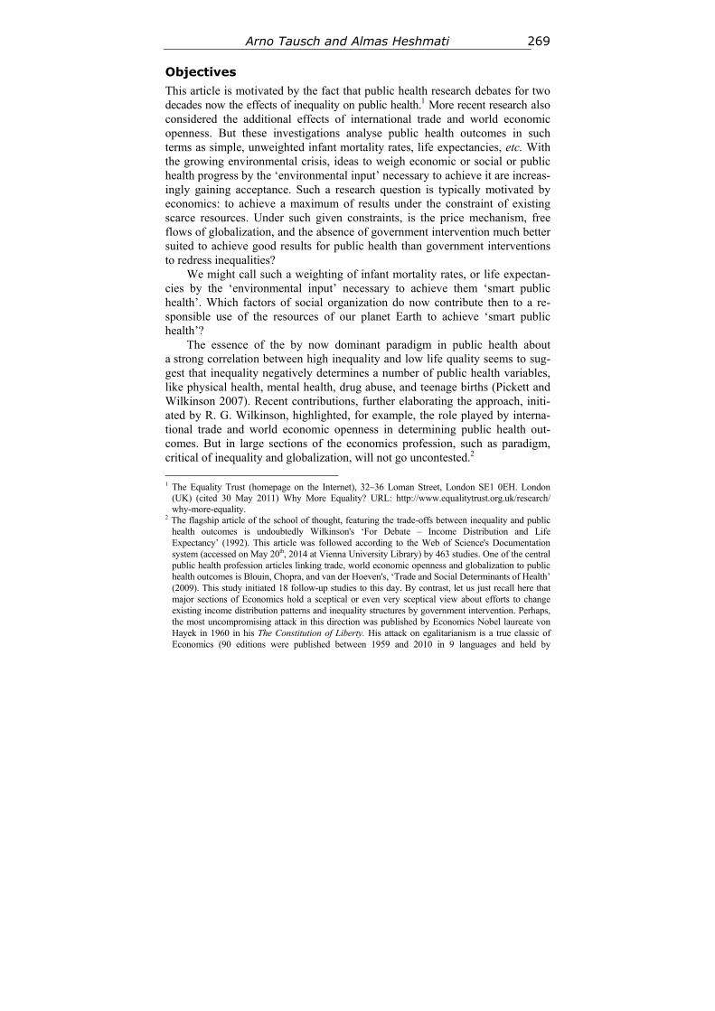
Arno Tausch and Almas Heshmati 269
Objectives
This article is motivated by the fact that public health research debates for two decades now the effects of inequality on public health.1 More recent research also considered the additional effects of international trade and world economic openness. But these investigations analyse public health outcomes in such terms as simple, unweighted infant mortality rates, life expectancies, etc. With the growing environmental crisis, ideas to weigh economic or social or public health progress by the ‘environmental input’ necessary to achieve it are increas-ingly gaining acceptance. Such a research question is typically motivated by economics: to achieve a maximum of results under the constraint of existing scarce resources. Under such given constraints, is the price mechanism, free flows of globalization, and the absence of government intervention much better suited to achieve good results for public health than government interventions to redress inequalities?
We might call such a weighting of infant mortality rates, or life expectan-cies by the ‘environmental input’ necessary to achieve them ‘smart public health’. Which factors of social organization do now contribute then to a re-sponsible use of the resources of our planet Earth to achieve ‘smart public health’?
The essence of the by now dominant paradigm in public health about a strong correlation between high inequality and low life quality seems to sug-gest that inequality negatively determines a number of public health variables, like physical health, mental health, drug abuse, and teenage births (Pickett and Wilkinson 2007). Recent contributions, further elaborating the approach, initi-ated by R. G. Wilkinson, highlighted, for example, the role played by interna-tional trade and world economic openness in determining public health out-comes. But in large sections of the economics profession, such as paradigm, critical of inequality and globalization, will not go uncontested.2
1 The Equality Trust (homepage on the Internet), 32–36 Loman Street, London SE1 0EH. London
(UK) (cited 30 May 2011) Why More Equality? URL: http://www.equalitytrust.org.uk/research/ why-more-equality.
2 The flagship article of the school of thought, featuring the trade-offs between inequality and public health outcomes is undoubtedly Wilkinson's ‘For Debate – Income Distribution and Life Expectancy’ (1992). This article was followed according to the Web of Science's Documentation system (accessed on May 20th, 2014 at Vienna University Library) by 463 studies. One of the central public health profession articles linking trade, world economic openness and globalization to public health outcomes is Blouin, Chopra, and van der Hoeven's, ‘Trade and Social Determinants of Health’ (2009). This study initiated 18 follow-up studies to this day. By contrast, let us just recall here that major sections of Economics hold a sceptical or even very sceptical view about efforts to change existing income distribution patterns and inequality structures by government intervention. Perhaps, the most uncompromising attack in this direction was published by Economics Nobel laureate von Hayek in 1960 in his The Constitution of Liberty. His attack on egalitarianism is a true classic of Economics (90 editions were published between 1959 and 2010 in 9 languages and held by
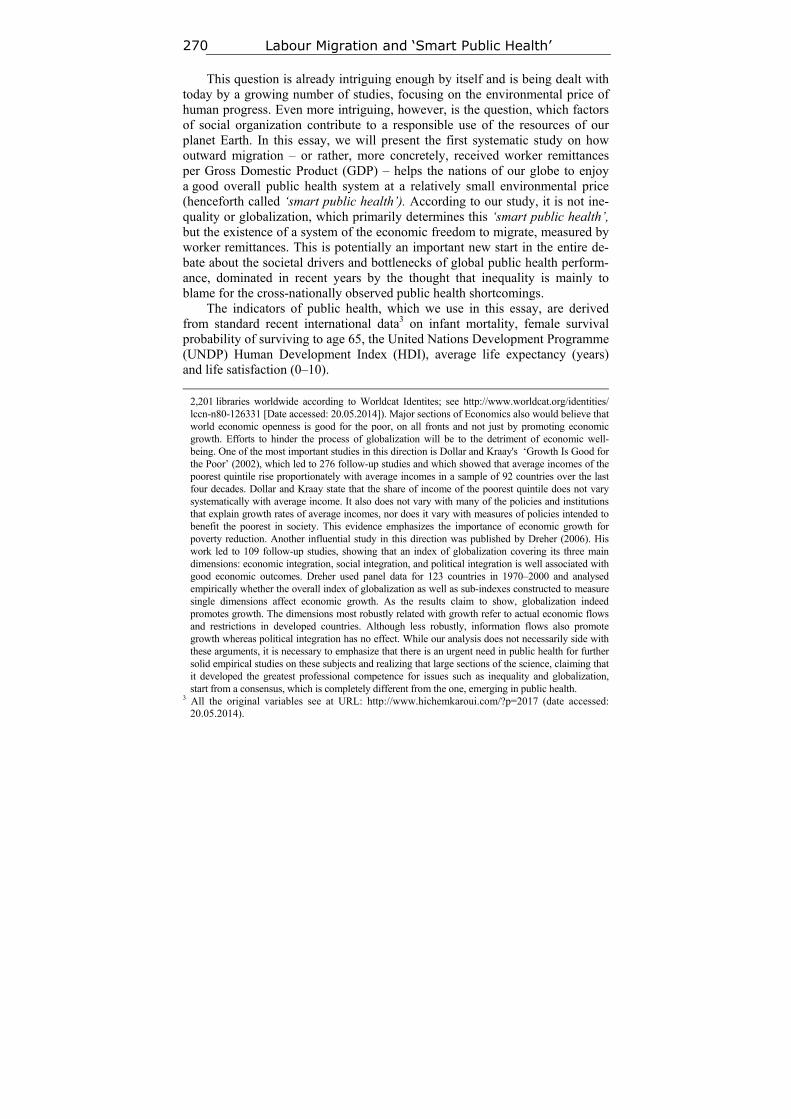
Labour Migration and ‘Smart Public Health’ 270
This question is already intriguing enough by itself and is being dealt with today by a growing number of studies, focusing on the environmental price of human progress. Even more intriguing, however, is the question, which factors of social organization contribute to a responsible use of the resources of our planet Earth. In this essay, we will present the first systematic study on how outward migration – or rather, more concretely, received worker remittances per Gross Domestic Product (GDP) – helps the nations of our globe to enjoy a good overall public health system at a relatively small environmental price (henceforth called ‘smart public health’). According to our study, it is not ine-quality or globalization, which primarily determines this ‘smart public health’, but the existence of a system of the economic freedom to migrate, measured by worker remittances. This is potentially an important new start in the entire de-bate about the societal drivers and bottlenecks of global public health perform-ance, dominated in recent years by the thought that inequality is mainly to blame for the cross-nationally observed public health shortcomings.
The indicators of public health, which we use in this essay, are derived from standard recent international data3 on infant mortality, female survival probability of surviving to age 65, the United Nations Development Programme (UNDP) Human Development Index (HDI), average life expectancy (years) and life satisfaction (0–10).
2,201 libraries worldwide according to Worldcat Identites; see http://www.worldcat.org/identities/ lccn-n80-126331 [Date accessed: 20.05.2014]). Major sections of Economics also would believe that world economic openness is good for the poor, on all fronts and not just by promoting economic growth. Efforts to hinder the process of globalization will be to the detriment of economic well-being. One of the most important studies in this direction is Dollar and Kraay's ‘Growth Is Good for the Poor’ (2002), which led to 276 follow-up studies and which showed that average incomes of the poorest quintile rise proportionately with average incomes in a sample of 92 countries over the last four decades. Dollar and Kraay state that the share of income of the poorest quintile does not vary systematically with average income. It also does not vary with many of the policies and institutions that explain growth rates of average incomes, nor does it vary with measures of policies intended to benefit the poorest in society. This evidence emphasizes the importance of economic growth for poverty reduction. Another influential study in this direction was published by Dreher (2006). His work led to 109 follow-up studies, showing that an index of globalization covering its three main dimensions: economic integration, social integration, and political integration is well associated with good economic outcomes. Dreher used panel data for 123 countries in 1970–2000 and analysed empirically whether the overall index of globalization as well as sub-indexes constructed to measure single dimensions affect economic growth. As the results claim to show, globalization indeed promotes growth. The dimensions most robustly related with growth refer to actual economic flows and restrictions in developed countries. Although less robustly, information flows also promote growth whereas political integration has no effect. While our analysis does not necessarily side with these arguments, it is necessary to emphasize that there is an urgent need in public health for further solid empirical studies on these subjects and realizing that large sections of the science, claiming that it developed the greatest professional competence for issues such as inequality and globalization, start from a consensus, which is completely different from the one, emerging in public health.
3 All the original variables see at URL: http://www.hichemkaroui.com/?p=2017 (date accessed: 20.05.2014).
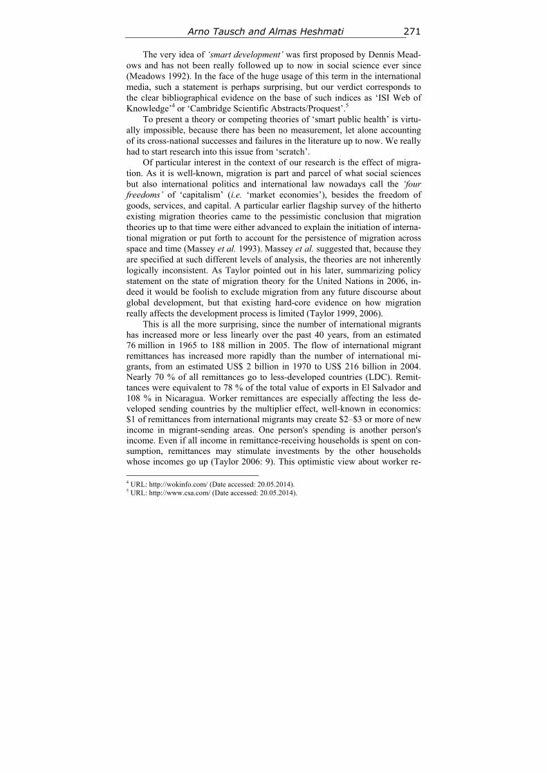
Arno Tausch and Almas Heshmati 271
The very idea of ‘smart development’ was first proposed by Dennis Mead-ows and has not been really followed up to now in social science ever since (Meadows 1992). In the face of the huge usage of this term in the international media, such a statement is perhaps surprising, but our verdict corresponds to the clear bibliographical evidence on the base of such indices as ‘ISI Web of Knowledge’4 or ‘Cambridge Scientific Abstracts/Proquest’.5
To present a theory or competing theories of ‘smart public health’ is virtu-ally impossible, because there has been no measurement, let alone accounting of its cross-national successes and failures in the literature up to now. We really had to start research into this issue from ‘scratch’.
Of particular interest in the context of our research is the effect of migra-tion. As it is well-known, migration is part and parcel of what social sciences but also international politics and international law nowadays call the ‘four freedoms’ of ‘capitalism’ (i.e. ‘market economies’), besides the freedom of goods, services, and capital. A particular earlier flagship survey of the hitherto existing migration theories came to the pessimistic conclusion that migration theories up to that time were either advanced to explain the initiation of interna-tional migration or put forth to account for the persistence of migration across space and time (Massey et al. 1993). Massey et al. suggested that, because they are specified at such different levels of analysis, the theories are not inherently logically inconsistent. As Taylor pointed out in his later, summarizing policy statement on the state of migration theory for the United Nations in 2006, in-deed it would be foolish to exclude migration from any future discourse about global development, but that existing hard-core evidence on how migration really affects the development process is limited (Taylor 1999, 2006).
This is all the more surprising, since the number of international migrants has increased more or less linearly over the past 40 years, from an estimated 76 million in 1965 to 188 million in 2005. The flow of international migrant remittances has increased more rapidly than the number of international mi-grants, from an estimated US$ 2 billion in 1970 to US$ 216 billion in 2004. Nearly 70 % of all remittances go to less-developed countries (LDC). Remit-tances were equivalent to 78 % of the total value of exports in El Salvador and 108 % in Nicaragua. Worker remittances are especially affecting the less de-veloped sending countries by the multiplier effect, well-known in economics: $1 of remittances from international migrants may create $2–$3 or more of new income in migrant-sending areas. One person's spending is another person's income. Even if all income in remittance-receiving households is spent on con-sumption, remittances may stimulate investments by the other households whose incomes go up (Taylor 2006: 9). This optimistic view about worker re-
4 URL: http://wokinfo.com/ (Date accessed: 20.05.2014). 5 URL: http://www.csa.com/ (Date accessed: 20.05.2014).
Labour Migration and ‘Smart Public Health’ 272
mittances is also supported in the well-received comparative international study by Ziesemer (2009).
Migration is thus seen in many social scientific approaches as a win-win situation (United Nations 2009; Williamson 2002). For several observers, among them Hatton and Williamson (2009), the ‘current hysteria’ about inward migration in many industrialized countries has no real basis. For them, the Third World has been undergoing an emigration life cycle since the 1960s, and, except for Africa, emigration rates have remained about equal or were even declining since a peak in the late 1980s and the early 1990s. The current economic crisis will serve only to accelerate those trends. Sanderson (2010) was one of the first consistent research attempts to bring in migration as a de-termining variable of social well-being. Contemporary levels of international migration in less-developed countries are raising new and important questions regarding the consequences of immigration for human welfare and well-being. However, there is little systematic cross-national evidence of how international migration affects human development levels in migrant-receiving countries in the less-developed world. The Sanderson paper addressed this gap in the litera-ture by assessing the impact of cumulative international migration flows on the human development index, the composite, well-known UNDP measure of ag-gregate well-being. A series of panel data models are estimated using a sample of less-developed countries for the period, 1970–2005. The results indicate that higher levels of international migration are associated with lower scores on the human development index, net of controls, but that the effect of international migration is relatively small.
Methods
To estimate the effects of migration on ‘smart public health’, we used a freely-available new cross-national comparative data set, which is publicly available on the Internet without any restrictions.6 This electronic data set offers Micro-soft EXCEL data and a list of the international standard sources, and a codebook in PDF format. It also offers an EXCEL file with the combined UNDP type development performance index, on which this study rests.
Each of these indicators (infant mortality, female survival probability of surviving to age 65, the United Nations Development Programme (UNDP) Human Development Index (HDI), average life expectancy (years) and life satisfaction (0–10) was standardized according to the well-known practice of the United Nations Human Development Programme on a scale, ranging from 0 (worst value) to 1 (best value) according to the formula:
),/()( minmaxminjjjijij XXXXZ (Eq. 1)
6 URL: http://www.hichemkaroui.com/?p=2017 (Date accessed: 20.05.2014).
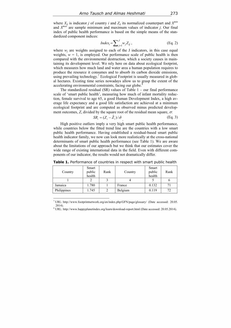
Arno Tausch and Almas Heshmati 273
where Xij is indicator j of country i and Zij its normalized counterpart and Xmin and Xmax are sample minimum and maximum values of indicator j. Our final index of public health performance is based on the simple means of the stan-dardized component indices:
ijJ
j ji ZwIndex
1, (Eq. 2)
where wj are weights assigned to each of the J indicators, in this case equal weights, w = 1, is employed. Our performance scale of public health is then compared with the environmental destruction, which a society causes in main-taining its development level. We rely here on data about ecological footprint, which measures how much land and water area a human population requires to produce the resource it consumes and to absorb its carbon dioxide emissions, using prevailing technology.7 Ecological Footprint is usually measured in glob-al hectares. Existing time series nowadays allow us to grasp the extent of the accelerating environmental constraints, facing our globe.8
The standardized residual (SR) values of Table 1 – our final performance scale of ‘smart public health’, measuring how much of infant mortality reduc-tion, female survival to age 65, a good Human Development Index, a high av-erage life expectancy and a good life satisfaction are achieved at a minimum ecological footprint and are computed as observed minus predicted develop-ment outcomes, Z, divided by the square root of the residual mean square, :
/)ˆ( iii ZZSR . (Eq. 3)
High positive outliers imply a very high smart public health performance, while countries below the fitted trend line are the countries with a low smart public health performance. Having established a residual-based smart public health indicator family, we now can look more realistically at the cross-national determinants of smart public health performance (see Table 1). We are aware about the limitations of our approach but we think that our estimates cover the wide range of existing international data in the field. Even with different com-ponents of our indicator, the results would not dramatically differ.
Table 1. Performance of countries in respect with smart public health
Country Smart public health
Rank Country Smart public health
Rank
1 2 3 4 5 6
Jamaica 1.780 1 France 0.132 71
Philippines 1.745 2 Belgium 0.119 72
7 URL: http://www.footprintnetwork.org/en/index.php/GFN/page/glossary/ (Date accessed: 20.05.
2014). 8 URL: http://www.happyplanetindex.org/learn/download-report.html (Date accessed: 20.05.2014).
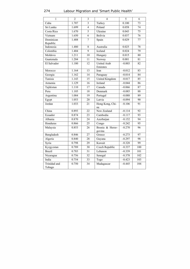
Labour Migration and ‘Smart Public Health’ 274
1 2 3 4 5 6
Cuba 1.707 3 Turkey 0.100 73
Sri Lanka 1.699 4 Poland 0.058 74
Costa Rica 1.670 5 Ukraine 0.043 75
Vietnam 1.650 6 Bolivia 0.037 76
Dominican Republic
1.488 7 Spain 0.029 77
Indonesia 1.480 8 Australia 0.025 78
Colombia 1.404 9 Iceland 0.024 79
Moldova 1.211 10 Hungary 0.015 80
Guatemala 1.204 11 Norway 0.001 81
El Salvador 1.180 12 United Arab Emirates
–0.003 82
Morocco 1.164 13 Iran –0.012 83
Georgia 1.162 14 Paraguay –0.014 84
Tunisia 1.143 15 United Kingdom –0.017 85
Armenia 1.129 16 Ireland –0.044 86
Tajikistan 1.110 17 Canada –0.066 87
Peru 1.105 18 Denmark –0.085 88
Argentina 1.084 19 Portugal –0.088 89
Egypt 1.053 20 Latvia –0.094 90
Jordan 1.033 21 Hong Kong, Chi-na
–0.106 91
China 0.893 22 New Zealand –0.114 92
Ecuador 0.874 23 Cambodia –0.117 93
Albania 0.870 24 Azerbaijan –0.152 94
Honduras 0.866 25 Congo –0.242 95
Malaysia 0.853 26 Bosnia & Herze-govina
–0.270 96
Bangladesh 0.846 27 Greece –0.273 97
Algeria 0.840 28 Guyana –0.297 98
Syria 0.798 29 Kuwait –0.328 99
Kyrgyzstan 0.789 30 Czech Republic –0.337 100
Brazil 0.783 31 Lebanon –0.339 101
Nicaragua 0.756 32 Senegal –0.378 102
India 0.754 33 Togo –0.423 103
Trinidad and Tobago
0.750 34 Madagascar –0.445 104
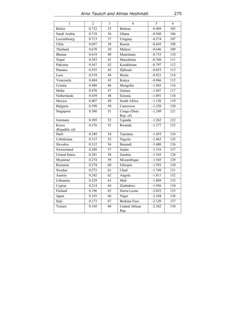
Arno Tausch and Almas Heshmati 275
1 2 3 4 5 6
Belize 0.732 35 Belarus –0.489 105
Saudi Arabia 0.718 36 Ghana –0.560 106
Luxembourg 0.713 37 Uruguay –0.574 107
Chile 0.697 38 Russia –0.645 108
Thailand 0.670 39 Malawi –0.646 109
Bhutan 0.619 40 Mauritania –0.733 110
Nepal 0.583 41 Macedonia –0.760 111
Pakistan 0.567 42 Kazakhstan –0.797 112
Panama 0.555 43 Djibouti –0.853 113
Laos 0.519 44 Benin –0.921 114
Venezuela 0.484 45 Kenya –0.966 115
Croatia 0.480 46 Mongolia –1.043 116
Malta 0.470 47 Guinea –1.047 117
Netherlands 0.439 48 Estonia –1.091 118
Mexico 0.407 49 South Africa –1.156 119
Bulgaria 0.398 50 Cameroon –1.220 120
Singapore 0.386 51 Congo (Dem. Rep. of)
–1.249 121
Germany 0.385 52 Uganda –1.262 122
Korea (Republic of)
0.376 53 Rwanda –1.277 123
Haiti 0.349 54 Tanzania –1.455 124
Uzbekistan 0.315 55 Nigeria –1.463 125
Slovakia 0.312 56 Burundi –1.480 126
Switzerland 0.288 57 Sudan –1.516 127
United States 0.281 58 Zambia –1.545 128
Myanmar 0.274 59 Mozambique –1.545 129
Romania 0.274 60 Ethiopia –1.593 130
Sweden 0.273 61 Chad –1.749 131
Austria 0.242 62 Angola –1.811 132
Lithuania 0.229 63 Mali –1.889 133
Cyprus 0.214 64 Zimbabwe –1.956 134
Finland 0.196 65 Sierra Leone –2.032 135
Japan 0.193 66 Niger –2.104 136
Italy 0.173 67 Burkina Faso –2.120 137
Yemen 0.145 68 Central African Rep.
–2.382 138
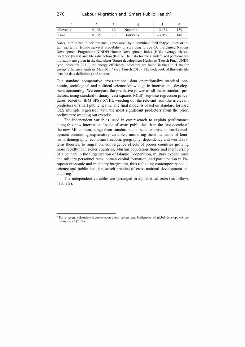
Labour Migration and ‘Smart Public Health’ 276
1 2 3 4 5 6 Slovenia 0.138 69 Namibia –2.457 139
Israel 0.135 70 Botswana –3.052 140
Notes: Public health performance is measured by a combined UNDP-type index of in-fant mortality, female survival probability of surviving to age 65, the United Nations Development Programme (UNDP) Human Development Index (HDI), average life ex-pectancy (years) and life satisfaction (0–10). The data for the standardized performance indicators are given in the data sheet ‘Smart development Heshmati Tausch Final UNDP type indicators 2011’, the energy efficiency indicators are found in the file ‘Data for energy efficiency analysis May 2011’ (see Tausch 2010). The codebook of this data file lists the data definitions and sources.
Our standard comparative cross-national data operationalize standard eco-nomic, sociological and political science knowledge in international develop-ment accounting. We compare the predictive power of all these standard pre-dictors, using standard ordinary least squares (OLS) stepwise regression proce-dures, based on IBM SPSS XVIII, weeding out the relevant from the irrelevant predictors of smart public health. The final model is based on standard forward OLS multiple regression with the most significant predictors from the prior, preliminary weeding out exercise.
The independent variables, used in our research to explain performance along this new international scale of smart public health in the first decade of the new Millennium, range from standard social science cross national devel-opment accounting explanatory variables, measuring the dimensions of femi-nism, demography, economic freedom, geography, dependency and world sys-tems theories, to migration, convergence effects of poorer countries growing more rapidly than richer countries, Muslim population shares and membership of a country in the Organization of Islamic Cooperation, military expenditures and military personnel rates, human capital formation, and participation in Eu-ropean economic and monetary integration, thus reflecting contemporary social science and public health research practice of cross-national development ac-counting.9
The independent variables are (arranged in alphabetical order) as follows (Table 2).
9 For a recent exhaustive argumentation about drivers and bottlenecks of global development see
Tausch et al. (2012).
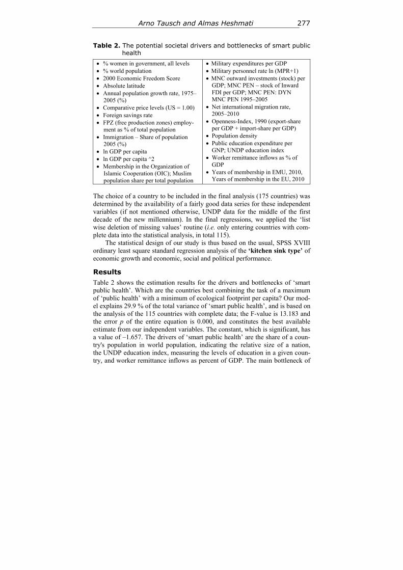
Arno Tausch and Almas Heshmati 277
Table 2. The potential societal drivers and bottlenecks of smart public health
% women in government, all levels % world population 2000 Economic Freedom Score Absolute latitude Annual population growth rate, 1975–
2005 (%) Comparative price levels (US = 1.00) Foreign savings rate FPZ (free production zones) employ-
ment as % of total population Immigration – Share of population
2005 (%) ln GDP per capita ln GDP per capita ^2 Membership in the Organization of
Islamic Cooperation (OIC); Muslim population share per total population
Military expenditures per GDP Military personnel rate ln (MPR+1) MNC outward investments (stock) per
GDP; MNC PEN – stock of Inward FDI per GDP; MNC PEN: DYN MNC PEN 1995–2005
Net international migration rate, 2005–2010
Openness-Index, 1990 (export-share per GDP + import-share per GDP)
Population density Public education expenditure per
GNP; UNDP education index Worker remittance inflows as % of
GDP Years of membership in EMU, 2010,
Years of membership in the EU, 2010
The choice of a country to be included in the final analysis (175 countries) was determined by the availability of a fairly good data series for these independent variables (if not mentioned otherwise, UNDP data for the middle of the first decade of the new millennium). In the final regressions, we applied the ‘list wise deletion of missing values’ routine (i.e. only entering countries with com-plete data into the statistical analysis, in total 115).
The statistical design of our study is thus based on the usual, SPSS XVIII ordinary least square standard regression analysis of the ‘kitchen sink type’ of economic growth and economic, social and political performance.
Results
Table 2 shows the estimation results for the drivers and bottlenecks of ‘smart public health’. Which are the countries best combining the task of a maximum of ‘public health’ with a minimum of ecological footprint per capita? Our mod-el explains 29.9 % of the total variance of ‘smart public health’, and is based on the analysis of the 115 countries with complete data; the F-value is 13.183 and the error p of the entire equation is 0.000, and constitutes the best available estimate from our independent variables. The constant, which is significant, has a value of –1.657. The drivers of ‘smart public health’ are the share of a coun-try's population in world population, indicating the relative size of a nation, the UNDP education index, measuring the levels of education in a given coun-try, and worker remittance inflows as percent of GDP. The main bottleneck of
Labour Migration and ‘Smart Public Health’ 278
‘smart public health’ is constituted by the crowding-out effect of public educa-tion expenditures on human development.
Table 3. OLS regression results of drivers and bottlenecks of smart public health (dependent variable is SR)
Independent Variable
B (un-standard-
ized regres-
sion coeffi-cient)
Standard error
Beta t-value
(Student's test)
Error probabil-
ity
Constant –1.657 0.348 –4.760 0.000
% world population 0.055 0.029 0.152 1.894 0.061
Public education expendi-ture per GNP
–0.097 0.042 –0.196 –2.283 0.024
UNDP education index 2.437 0.430 0.478 5.666 0.000
Worker remittance inflows as % of GDP
0.044 0.010 0.352 4.461 0.000
Memorandum item: statis-tical properties of the equation
Adj. R^2 Df. F Error prob. of the entire
equation
29.900 114 13.183 0.000
Conclusion
Our residuals-based reformulation of smart public health realistically captures the trade-off between Global Ecological Footprint per capita and development performance and offers us a better idea about smart public health performance at different stages of socio-economic development.10 Our results show that tra-ditional indicators of economic globalization and also inequality have little in-fluence on combined smart public health performance, but that hitherto ne-glected elements of social science theories, such as migration, gain in impor-tance. Also such factors as the demographic weight of a country and scale ef-fects of public health provision, and education cannot be overlooked. In con-trast to most of the current thinking on the issue, we can show that levels of public education expenditures crowd out health performance, while levels of achieved education, measured by the UNDP education index, have a beneficial
10 The inclusion of the UNDP-standardized equality score (= performance in avoiding a high ratio of
income differences between the richest 20 % and the poorest 20 %) only has a minor effect on our results: for the 106 countries with complete data. The equality score achieves an error probability of 13.5 %. As expected, equality has a positive effect on smart public health, but the effect is far smaller than existing approaches would suggest.
Arno Tausch and Almas Heshmati 279
effect on ‘smart public health’. True enough, we have to state that worker re-mittances redistribute global well-being and the achievement of good public health outcomes at relatively low ecological resource use to the countries of the ‘global South’ and away from the rich democracies of the OECD.
We are aware that our answers to the questions raised in this article might be incomplete. But we hope to have provided at least some preliminary guiding posts for further research on this important subject how the four economic free-doms affect smart public health and to have shown that primarily not inequal-ity, but migration matters for public health. If we have expressed this perspec-tive sufficiently clear, then our essay already achieved its aim. Further research might concentrate on such issues as ‘smart infant mortality reduction’ or ‘smart life expectancy’.
References
Blouin C., Chopra M., and van der Hoeven R. 2009. Trade and Social Determinants of Health. The Lancet 373(9662): 502–507.
Dollar D., and Kraay A. 2002. Growth is Good for the Poor. Journal of Economic Growth 7(3): 195–225.
Dreher A. 2006. Does Globalization Affect Growth? Evidence from a New Index of Globalization. Applied Economics 38(10): 1091–1110.
Hatton T. J., and Williamson J. A. Vanishing Third World Emigrants? Harvard Uni-versity, Department of Economics, 2009. URL: http://ideas.repec.org/p/auu/ dpa-per/606.html. Date accessed: 20.05. 2014.
von Hayek F. A. 1960. The Constitution of Liberty. Chicago, IL: University of Chicago Press.
Massey D. S et al. 1993. Theories of International Migration: A Review and Appraisal. Population and Development Review 19(3): 431–466.
Meadows D. H. 1992. Smart Development, Not Dumb Growth. Technology Review 95(6): 68–89.
Pickett K. E., and Wilkinson R. G. 2007. Child Wellbeing and Income Inequality in Rich Societies: Ecological Cross Sectional Study. BMJ 335. DOI: 10.1136/bmj. 39377.580162.55.
Sanderson M. 2010. International Migration and Human Development in Destination Countries: A Cross-National Analysis of Less-Developed Countries, 1970–2005. Social Indicators Research 96(1): 59–83.
Taylor J. E. 1999. The New Economics of Labour Migration and the Role of Remit-tances in the Migration Process. International Migration 37(1): 63–88.
Taylor J. E. 2006. International Migration and Economic Development. UN/POP/ MIG/SYMP/2006/09. International Symposium on International Migration and De-velopment, Population Division, Department of Economic and Social Affairs, Unit-ed Nations Secretariat, Turin, Italy, 28–30 June 2006. URL: http://www.ncbi. nlm.nih.gov/pubmed/12322077. Date accessed: 27.02.2012.

Labour Migration and ‘Smart Public Health’ 280
Tausch A. 2010. 41 Indicators of Development – A Public Access Codebook for the International Development Research Community. URL: http://www.hichemkaroui. com/?p=2017. Date accessed: 27.02.2012.
Tausch A., Heshmati A., and Brand U. 2012. Globalization, the Human Condition and Sustainable Development in the 21st Century. Cross-National Perspectives and European Implications. London – Delhi – New York: Anthem Press.
United Nations 2009. United Nations Human Development Report. New York – Ox-ford: Oxford University Press.
Williamson J. A. 2002. Is Protection Bad for Growth? Will Globalization Last? Look-ing for Answers in History. Presented at the 13th IEHA Congress, Buenos Aires, Au-gust 22–26, 2002. Draft Date: June 2002. URL: http://www.economics.harvard. edu/faculty/williamson/jwilliamworkingpapers. Date accessed: 20.05.2014.
Wilkinson R. G. 1992. For Debate – Income Distribution and Life Expectancy. British Medical Journal 304(6820): 165–168.
Ziesemer T. H. W. 2009. Worker Remittances and Growth: The Physical and Human Capital Channels. Jahrbücher für Nationalökonomie und Statistik 229(6): 743–773.
History & Mathematics: Trends and Cycles 281–299
281
9
Is Geography ‘Dead’ or ‘Destiny’ in a Globalizing World?
A Network Analysis and Latent Space Modeling Approach
of the World Trade Network
Anthony Howell
Abstract
Drawing on advancements made in network analysis, statistical modeling and computer science, this paper employs latent space modeling techniques to ex-plore the role of geography in the global trade economy. Latent space models postulate that the probability of a link between pairs of actors depends on the distance between them in unobserved Euclidean social space and on observed covariates. Using probabilistic models, I investigate the effect that distance has on influencing trade ties in social space, while also controlling for several co-variates, including region-based homophily (a proxy for regionalization), tran-sitivity and country wealth. The findings are posited within the ‘Geography is Dead’ thesis and reveal that the distance-destroying result attributed to global-ization may be over-estimated in the global trade economy.
Keywords: network analysis, latent space model, world trade network, geo-graphy, regionalization, globalization.
1. Introduction
Since Toffler (1970) first argued that place is no longer an important determi-nant due to the evolution of transport and communication systems, numerous scholars have speculated the ‘death of geography’, giving rise to a heated de-bate (Ohmae 1990, 1995; Friedmann 1995). O'Brien (1992) proclaimed that the globalization era equates to ‘the end of geography’, because geographical loca-tion no longer matters for economic development due to the increasing rate of globalization. In this context, globalization is defined as ‘the deepening integra-tion of global economic activity facilitated by the rapid development of infor-mation and communications technology and the underlying trend towards liber-alization in trade and investment’ (Staples 2007: 99).
Is Geography ‘Dead’ or ‘Destiny’ in a Globalizing World? 282
Despite the ‘geography is dead’ claims, many notable (economic) geogra-phers emphasize the critical role of geography in trade, as well as in innovation, knowledge and development (Krugman 1993; Yeung 1998; Massey 1984, 1999; Morgan 2004). It is well known that the effects of globalization are not distributed uniformly throughout the global economy, and there are place- and region-based variations that require a geographical lens in order to understand issues of unequal development (Warwick 2005). Moreover, the growing forms of regionalization shed further evidence that geography does matter for trade and economic development. Regionalization is defined here as a process, ‘whereby economic interaction, such as flows of goods and capital, increase faster among countries within a particular geographical area than between those countries and others outside the area’ (Moore 2007: 36).
In the present paper, I apply latent space modeling – developed by Hoff et al. (2002) – to test the ‘geography is dead’ thesis. Hoff et al. (2002) postulate that the probability of a link between pairs of actors depends on the distance between them in unobserved Euclidean social space and on observed covari-ates. Using the latent space modeling approach, I investigate the effect that dis-tance has on trade ties in latent space, while also controlling for several covari-ates, including region-based homophily (a proxy for regionalization), transitiv-ity and country wealth.
Stochastic models can be used to identify the specific processes that have led the network to its particular configuration. Both the gravity model and the exponential random graph model (ERGM) are possible approaches to test the relationship between geography and trade. Aside from weak theoretical backing, another main shortcoming with these approaches is that they assume independence among all trade linkages between country pairs. In reality, it is very likely that there is inherent dependency between ties (Shortreed et al. 2006). For example, if South Africa and Brazil are trade partners, and China and Brazil are trade partners, then it is more likely that South Africa and China are trade partners then it is if these previous trade relationships did not exist.
By implementing proxies to take into account second- and third-order de-pendences in the network, the latent space model is one method to deal with this dependency.
This paper attempts to add to the growing literature on the World Trade Network (WTN), as well as to test the ‘death of geography’ thesis, by statisti-cally analyzing the role of geography and trade integration using latent space stochastic models. To carry out these objectives, I estimate several simple latent space models to capture the relationship between distance and the likelihood of two countries establishing a trade partnership in the WTN, while also taking into account higher order dependencies in the network. Results from the analy-sis support regionalization, in favor of the ‘geography is destiny’ thesis (Dieter 2007), implying that proponents of the ‘geography is dead’ overestimate the distance-destroying effects of globalization on the global trade economy.
Anthony Howell 283
The outline of this paper is as follows. In the subsequent section, I provide a brief background on relevant network analysis studies. In Section 3, I discuss issues related to building, specifying and representing the trade network. In Section 4, I provide an overview of the main network statistics and network properties commonly used to infer patterns in the trade network. Specifically, I consider connectivity, centrality, clustering and hierarchy, as well as homo-phily and transitivity. In Section 5, I specify several latent space models and test the principles of propinquity, homophily and transitivity. Lastly, Section 6 concludes with some final remarks.
2. Background
Due to advancements in physics and computer science, network analysis is in-creasingly relied upon to study the world trade network and is a powerful tool that can be used to reveal topological properties, as well as the underlying structure of the trade network (Fagiolo et al. 2009; Reyes et al. 2007, 2010). For instance, network analysis applications of the world trade network (WTN) have most notably addressed two major questions: (1) does the trade network follow a core-periphery structure (Clark 2008, 2010; Kali and Reyes 2007); and (2) do global elites tend to trade among themselves and what are the effects of international trade on economic growth (Bhattacharya et al. 2008; Serrano 2008; Fagiolo et al. 2009).
Although comparatively underdeveloped, network analysis has also been employed to investigate the role of geography in the global trade economy. Kim and Shin (2002) argue that network analysis can naturally be extended from dependency/world-systems theory to test the globalization vs. regionaliza-tion thesis that indirectly tests the role of geography by determining whether countries in the network are globalizing or regionalizing (Aggarwal and Koo 2005; Kim and Shin 2002; He and Deem 2010).
Findings from network analysis contribute to the debate over whether re-gionalization is a stepping stone or stumbling block to globalization (Bhagwati et al. 1999). On the one hand, some scholars believe that regionalization is a transitory step that some countries pursue to become more competitive on the global market, eventually promoting globalization and rendering geography unimportant. On the other hand, other scholars suggest that regionalization im-pedes globalization by hurting the welfare of non-member countries and lead-ing to inefficient production strategies that may work at the regional scale but not at the global scale.
For instance, Kastelle et al. (2006) provides evidence that the ‘movement of trade, capital and people is a geographically heterogeneous and historically episodic process and can be interpreted to support regionalization rather than globalization’. The authors' finding is significant because it highlights the pow-er of geography to influence trade outcomes; even in an ever-increasing global-
Is Geography ‘Dead’ or ‘Destiny’ in a Globalizing World? 284
ized world, countries still pursue regional trade integration policies with nearby countries.
Conversely, Kim and Shin (2002) argue that globalization and regionaliza-tion are not necessarily competitive, but complementary processes. From 1959–1996, the authors show that the WTN became globalized (overall network den-sity increased significantly), while it also became regionalized (intraregional density also significantly increased). Based on their findings, the authors sug-gest that regionalization does not jeopardize globalization; rather the two proc-esses are complimentary and can coincide with one another.
While the authors' findings have far reaching implications into the effects of regionalization and globalization on the global economy, the findings are predi-cated merely on descriptive statistics, in this case, a network statistic called node degree. Node degree measures the probability of a randomly chosen vertex to have k-connections to other vertices and provides a summary of a node's overall activity.11 The problem with this network statistic, like any other descriptive statistic, is that no statistical model is used to control for other potential inter-mediating variables that may influence the outcome of a trade tie being estab-lished.
Most of the literature on the WTN only examines the network's summary statistics to track topological changes, and few attempts are made to statistically analyze the trade network using stochastic models (notable exceptions are Gar-laschelli and Loffredo 2005; Garlaschelli et al. 2007). Fitting statistical models to networks, in general, is still in its infancy stages due to the complexity of modeling networks and the high level of computation that is required (Hunter and Handcock 2005). It is not surprising, therefore, that the WTN literature has only recently begun to be modeled; despite the complicated nature of the WTN, pertinent topological properties of the global trade system can and should be extracted through modeling the system as a network (Serrano 2008).
3. The Network Data: Specification and Representation
Bilateral trade data are extracted from the United Nations COMTRADE data-base. Data for GDP per capita and the trade/GDP share are extracted from Penn World Table 6.2 (for a country listing, see Appendix). In the trade network, countries represent nodes and the links between two countries are their shared imports and exports. If a trade tie is not present, then yij = 0. The data offer in-formation on both exports and imports, however, I use only import data be-cause previous scholars suggest that these figures are more accurate than export figures (Kim and Shin 2002).
1 Node degree is discussed in greater detail in Section 4.
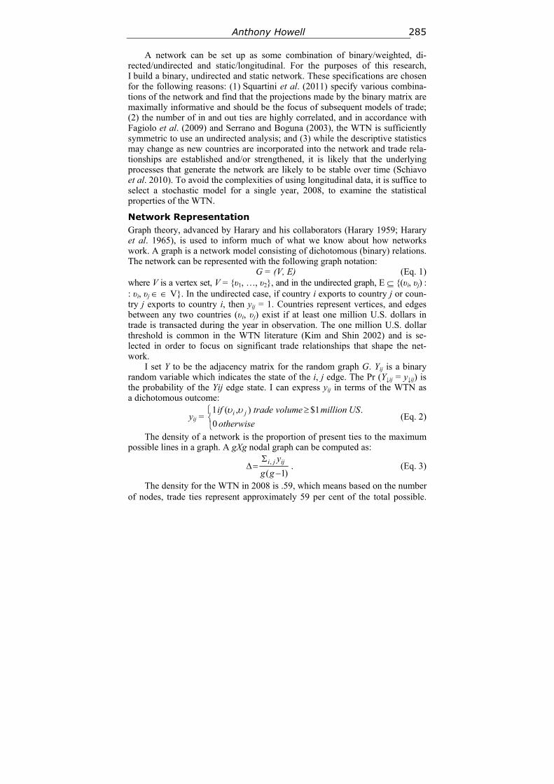
Anthony Howell 285
A network can be set up as some combination of binary/weighted, di-rected/undirected and static/longitudinal. For the purposes of this research, I build a binary, undirected and static network. These specifications are chosen for the following reasons: (1) Squartini et al. (2011) specify various combina-tions of the network and find that the projections made by the binary matrix are maximally informative and should be the focus of subsequent models of trade; (2) the number of in and out ties are highly correlated, and in accordance with Fagiolo et al. (2009) and Serrano and Boguna (2003), the WTN is sufficiently symmetric to use an undirected analysis; and (3) while the descriptive statistics may change as new countries are incorporated into the network and trade rela-tionships are established and/or strengthened, it is likely that the underlying processes that generate the network are likely to be stable over time (Schiavo et al. 2010). To avoid the complexities of using longitudinal data, it is suffice to select a stochastic model for a single year, 2008, to examine the statistical properties of the WTN.
Network Representation Graph theory, advanced by Harary and his collaborators (Harary 1959; Harary et al. 1965), is used to inform much of what we know about how networks work. A graph is a network model consisting of dichotomous (binary) relations. The network can be represented with the following graph notation:
G = (V, E) (Eq. 1) where V is a vertex set, V = {υ1, …, υ2}, and in the undirected graph, E {(υi, υj) : : υi, υj V}. In the undirected case, if country i exports to country j or coun-try j exports to country i, then yij = 1. Countries represent vertices, and edges between any two countries (υi, υj) exist if at least one million U.S. dollars in trade is transacted during the year in observation. The one million U.S. dollar threshold is common in the WTN literature (Kim and Shin 2002) and is se-lected in order to focus on significant trade relationships that shape the net-work.
I set Y to be the adjacency matrix for the random graph G. Yij is a binary random variable which indicates the state of the i, j edge. The Pr (Y↓ij = y↓ij) is the probability of the Yij edge state. I can express yij in terms of the WTN as a dichotomous outcome:
yij =
otherwise
USmillionvolumetradeif ji
0
.1$),(1 (Eq. 2)
The density of a network is the proportion of present ties to the maximum possible lines in a graph. A gXg nodal graph can be computed as:
)1(,
gg
yijji . (Eq. 3)
The density for the WTN in 2008 is .59, which means based on the number of nodes, trade ties represent approximately 59 per cent of the total possible.
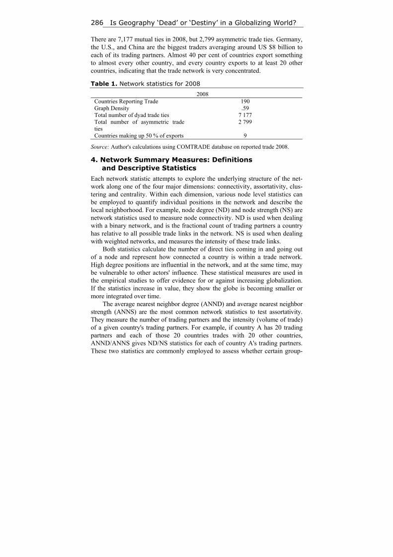
Is Geography ‘Dead’ or ‘Destiny’ in a Globalizing World? 286
There are 7,177 mutual ties in 2008, but 2,799 asymmetric trade ties. Germany, the U.S., and China are the biggest traders averaging around US $8 billion to each of its trading partners. Almost 40 per cent of countries export something to almost every other country, and every country exports to at least 20 other countries, indicating that the trade network is very concentrated.
Table 1. Network statistics for 2008
2008 Countries Reporting Trade 190 Graph Density .59 Total number of dyad trade ties 7 177 Total number of asymmetric trade ties
2 799
Countries making up 50 % of exports 9
Source: Author's calculations using COMTRADE database on reported trade 2008.
4. Network Summary Measures: Definitions and Descriptive Statistics
Each network statistic attempts to explore the underlying structure of the net-work along one of the four major dimensions: connectivity, assortativity, clus-tering and centrality. Within each dimension, various node level statistics can be employed to quantify individual positions in the network and describe the local neighborhood. For example, node degree (ND) and node strength (NS) are network statistics used to measure node connectivity. ND is used when dealing with a binary network, and is the fractional count of trading partners a country has relative to all possible trade links in the network. NS is used when dealing with weighted networks, and measures the intensity of these trade links.
Both statistics calculate the number of direct ties coming in and going out of a node and represent how connected a country is within a trade network. High degree positions are influential in the network, and at the same time, may be vulnerable to other actors' influence. These statistical measures are used in the empirical studies to offer evidence for or against increasing globalization. If the statistics increase in value, they show the globe is becoming smaller or more integrated over time.
The average nearest neighbor degree (ANND) and average nearest neighbor strength (ANNS) are the most common network statistics to test assortativity. They measure the number of trading partners and the intensity (volume of trade) of a given country's trading partners. For example, if country A has 20 trading partners and each of those 20 countries trades with 20 other countries, ANND/ANNS gives ND/NS statistics for each of country A's trading partners. These two statistics are commonly employed to assess whether certain group-
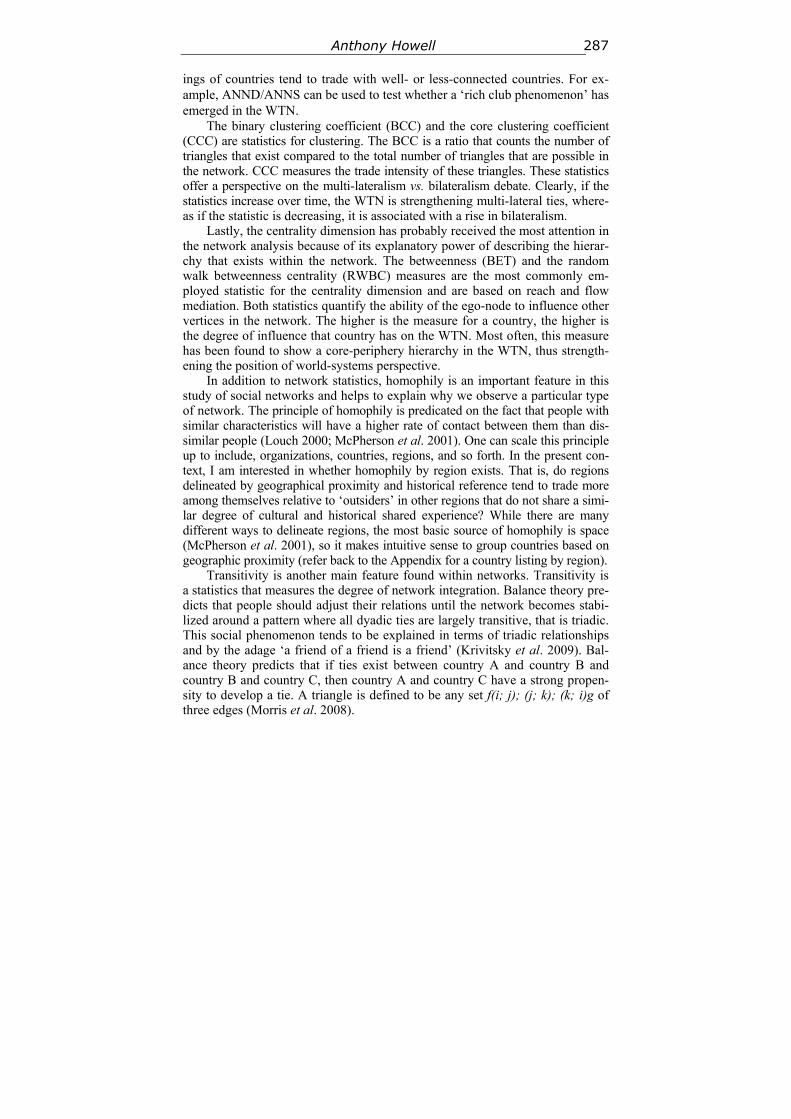
Anthony Howell 287
ings of countries tend to trade with well- or less-connected countries. For ex-ample, ANND/ANNS can be used to test whether a ‘rich club phenomenon’ has emerged in the WTN.
The binary clustering coefficient (BCC) and the core clustering coefficient (CCC) are statistics for clustering. The BCC is a ratio that counts the number of triangles that exist compared to the total number of triangles that are possible in the network. CCC measures the trade intensity of these triangles. These statistics offer a perspective on the multi-lateralism vs. bilateralism debate. Clearly, if the statistics increase over time, the WTN is strengthening multi-lateral ties, where-as if the statistic is decreasing, it is associated with a rise in bilateralism.
Lastly, the centrality dimension has probably received the most attention in the network analysis because of its explanatory power of describing the hierar-chy that exists within the network. The betweenness (BET) and the random walk betweenness centrality (RWBC) measures are the most commonly em-ployed statistic for the centrality dimension and are based on reach and flow mediation. Both statistics quantify the ability of the ego-node to influence other vertices in the network. The higher is the measure for a country, the higher is the degree of influence that country has on the WTN. Most often, this measure has been found to show a core-periphery hierarchy in the WTN, thus strength-ening the position of world-systems perspective.
In addition to network statistics, homophily is an important feature in this study of social networks and helps to explain why we observe a particular type of network. The principle of homophily is predicated on the fact that people with similar characteristics will have a higher rate of contact between them than dis-similar people (Louch 2000; McPherson et al. 2001). One can scale this principle up to include, organizations, countries, regions, and so forth. In the present con-text, I am interested in whether homophily by region exists. That is, do regions delineated by geographical proximity and historical reference tend to trade more among themselves relative to ‘outsiders’ in other regions that do not share a simi-lar degree of cultural and historical shared experience? While there are many different ways to delineate regions, the most basic source of homophily is space (McPherson et al. 2001), so it makes intuitive sense to group countries based on geographic proximity (refer back to the Appendix for a country listing by region).
Transitivity is another main feature found within networks. Transitivity is a statistics that measures the degree of network integration. Balance theory pre-dicts that people should adjust their relations until the network becomes stabi-lized around a pattern where all dyadic ties are largely transitive, that is triadic. This social phenomenon tends to be explained in terms of triadic relationships and by the adage ‘a friend of a friend is a friend’ (Krivitsky et al. 2009). Bal-ance theory predicts that if ties exist between country A and country B and country B and country C, then country A and country C have a strong propen-sity to develop a tie. A triangle is defined to be any set f(i; j); (j; k); (k; i)g of three edges (Morris et al. 2008).
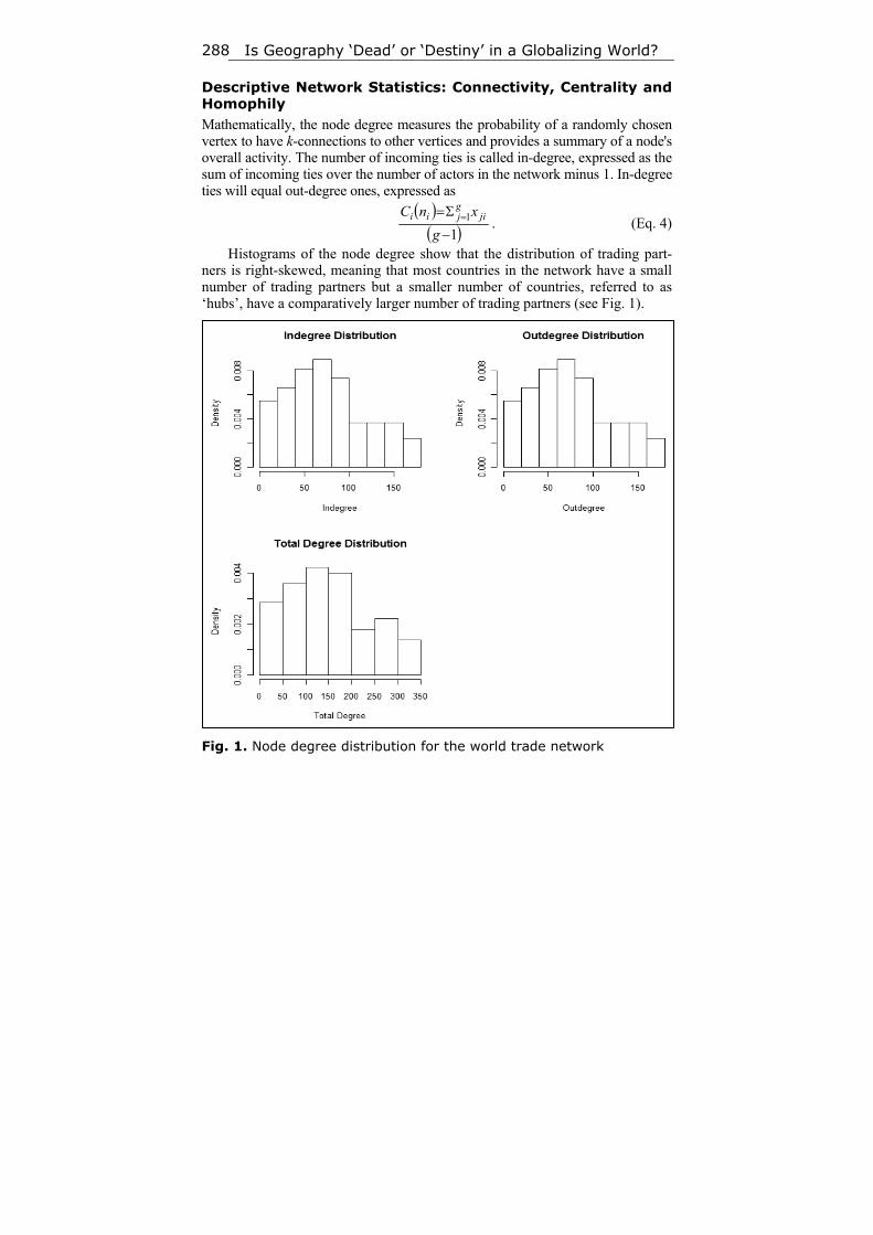
Is Geography ‘Dead’ or ‘Destiny’ in a Globalizing World? 288
Descriptive Network Statistics: Connectivity, Centrality and Homophily Mathematically, the node degree measures the probability of a randomly chosen vertex to have k-connections to other vertices and provides a summary of a node's overall activity. The number of incoming ties is called in-degree, expressed as the sum of incoming ties over the number of actors in the network minus 1. In-degree ties will equal out-degree ones, expressed as
1
1
g
xnC jigjii
. (Eq. 4)
Histograms of the node degree show that the distribution of trading part-ners is right-skewed, meaning that most countries in the network have a small number of trading partners but a smaller number of countries, referred to as ‘hubs’, have a comparatively larger number of trading partners (see Fig. 1).
Fig. 1. Node degree distribution for the world trade network
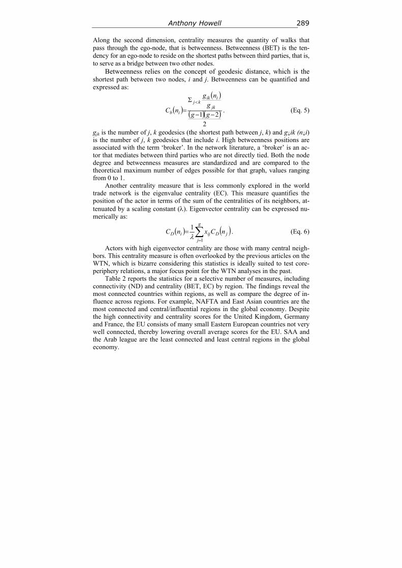
Anthony Howell 289
Along the second dimension, centrality measures the quantity of walks that pass through the ego-node, that is betweenness. Betweenness (BET) is the ten-dency for an ego-node to reside on the shortest paths between third parties, that is, to serve as a bridge between two other nodes.
Betweenness relies on the concept of geodesic distance, which is the shortest path between two nodes, i and j. Betweenness can be quantified and expressed as:
2
21
gg
g
ng
nC jk
iikkj
ib . (Eq. 5)
gjk is the number of j, k geodesics (the shortest path between j, k) and gik (ni) is the number of j, k geodesics that include i. High betweenness positions are associated with the term ‘broker’. In the network literature, a ‘broker’ is an ac-tor that mediates between third parties who are not directly tied. Both the node degree and betweenness measures are standardized and are compared to the theoretical maximum number of edges possible for that graph, values ranging from 0 to 1.
Another centrality measure that is less commonly explored in the world trade network is the eigenvalue centrality (EC). This measure quantifies the position of the actor in terms of the sum of the centralities of its neighbors, at-tenuated by a scaling constant (). Eigenvector centrality can be expressed nu-merically as:
jD
g
jijiD nCxnC
1
1
. (Eq. 6)
Actors with high eigenvector centrality are those with many central neigh-bors. This centrality measure is often overlooked by the previous articles on the WTN, which is bizarre considering this statistics is ideally suited to test core-periphery relations, a major focus point for the WTN analyses in the past.
Table 2 reports the statistics for a selective number of measures, including connectivity (ND) and centrality (BET, EC) by region. The findings reveal the most connected countries within regions, as well as compare the degree of in-fluence across regions. For example, NAFTA and East Asian countries are the most connected and central/influential regions in the global economy. Despite the high connectivity and centrality scores for the United Kingdom, Germany and France, the EU consists of many small Eastern European countries not very well connected, thereby lowering overall average scores for the EU. SAA and the Arab league are the least connected and least central regions in the global economy.

Is Geography ‘Dead’ or ‘Destiny’ in a Globalizing World? 290
Table 2. Connectivity and Centrality Measures by Region and Select Countries
Region ND BET EC 1 2 3 4
NAFTA (n = 3) 279.3 218.9 .107 USA 346 439.39 .121 CAN 284 186.2 .11 MEX 208 31.2 .09 EU 2 (n = 40) 210.3 103.8 .084 UKG 344 522.9 .12 GFR 340 376.9 .121 FRN 338 304.3 .11 East Asia (n = 5) 246 177.7 .094 JPN 342 477.7 .12 China 332 270.8 .121 ROK 310 177.21 .11 ECE (n = 11) 156.2 27.4 .079 RUS 278 104 .11 UKR 276 109 .12 BLR 194 39.5 .082 ASEAN (n = 10) 191.4 78.5 .079 THI 304 233.7 .113 MAL 298 170.4 .113 INS 292 144.4 .112 SAA (n = 9) 136.7 45.6 .058 IND 314 222.7 .116
PAK 262 107.6 .102 BNG 196 57.68 .082 Arab League (n = 17) 155.4 24.4 .068 SAU 234 90.2 .093 ISR 232 65.3 .095 UAE 218 62.1 .09 Pacific Islands (n = 13) 80 38.04 .033 AUL 294 246.7 .11 AUS 266 114.12 .106 NEW 220 120.7 .09 Latin America (31) 132.9 21.2 .059 BRA 294 175.2 .11 ARG 244 65.3 .101 RUM 242 69.4 .1 African Union (50) 106.3 11.2 .049 SAF 280 131.2 .109 EGY 228 49.5 .096
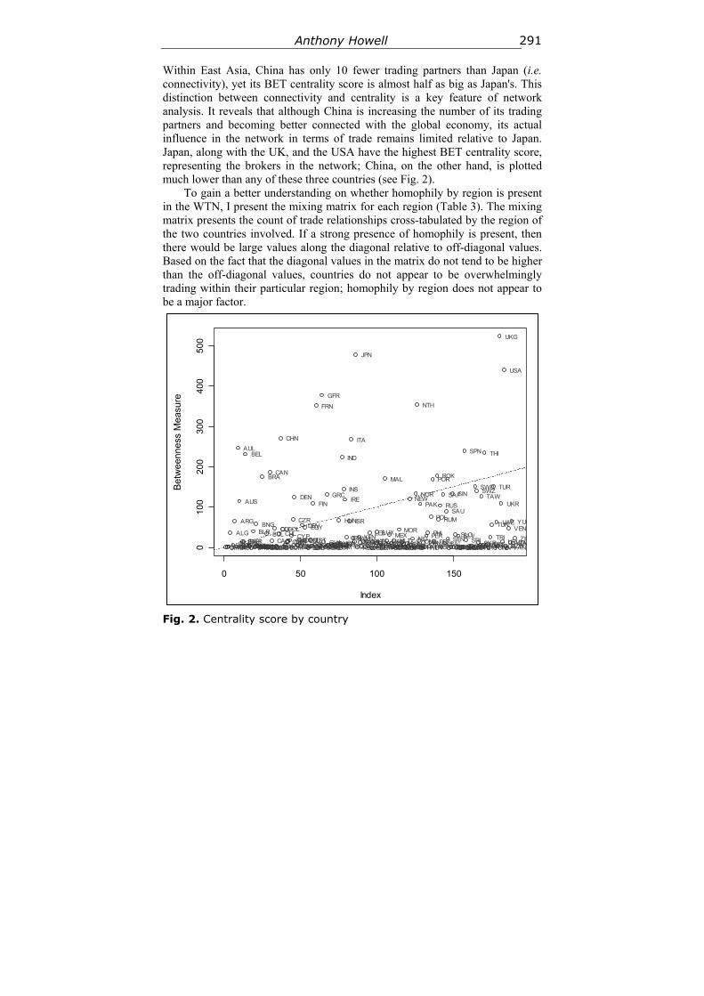
Anthony Howell 291
Within East Asia, China has only 10 fewer trading partners than Japan (i.e. connectivity), yet its BET centrality score is almost half as big as Japan's. This distinction between connectivity and centrality is a key feature of network analysis. It reveals that although China is increasing the number of its trading partners and becoming better connected with the global economy, its actual influence in the network in terms of trade remains limited relative to Japan. Japan, along with the UK, and the USA have the highest BET centrality score, representing the brokers in the network; China, on the other hand, is plotted much lower than any of these three countries (see Fig. 2).
To gain a better understanding on whether homophily by region is present in the WTN, I present the mixing matrix for each region (Table 3). The mixing matrix presents the count of trade relationships cross-tabulated by the region of the two countries involved. If a strong presence of homophily is present, then there would be large values along the diagonal relative to off-diagonal values. Based on the fact that the diagonal values in the matrix do not tend to be higher than the off-diagonal values, countries do not appear to be overwhelmingly trading within their particular region; homophily by region does not appear to be a major factor.
Fig. 2. Centrality score by country
0 50 100 150
01
00
20
03
00
40
05
00
Index
Be
twe
en
ess
Me
asu
re
AABAFGALB
ALG
ANDANG
ARG
ARM
AUL
AUS
AZEBAHBAR
BEL
BENBFOBHMBHU
BLR
BLZ
BNG
BOLBOSBOT
BRA
BRUBUI
BUL
CAM
CAN
CAOCAP
CDI
CENCHA
CHL
CHN
COL
COMCONCOSCROCUBCYP
CZR
DEN
DJIDMADOMDRC
DRV
ECU
EGY
EQGERIESTETH
FIN
FJI
FRN
FSMGABGAM
GFR
GHAGNB
GRC
GRGGRNGUAGUIGUYHAIHON
HUN
ICE
IND
INS
IRE
IRNIRQ
ISR
ITA
JAMJOR
JPN
KBI
KENKUWKYRKZKLAOLATLBR
LEB
LESLIBLIELIT
LUX
MAAMACMADMAG
MAL
MASMAW
MEXMLDMLIMLTMNCMON
MOR
MSIMYAMZMNAMNAUNEP
NEW
NICNIGNIR
NOR
NTH
OMA
PAK
PALPANPAR
PERPHI
PNG
POL
POR
PRKQAT
ROK
RUM
RUS
RWA
SAF
SAL
SAU
SENSEYSIE
SIN
SKN
SLO
SLU
SLV
SNMSOLSOM
SPN
SRISTPSUDSURSVGSWA
SWDSWZ
SYRTAJ
TAW
TAZ
THI
TKMTOGTON
TRI
TUN
TUR
TUV
UAE
UGA
UKG
UKR
URU
USA
UZBVAN
VEN
YEM
YUG
ZAZIM
Bet
wee
nnes
s M
eas
ure
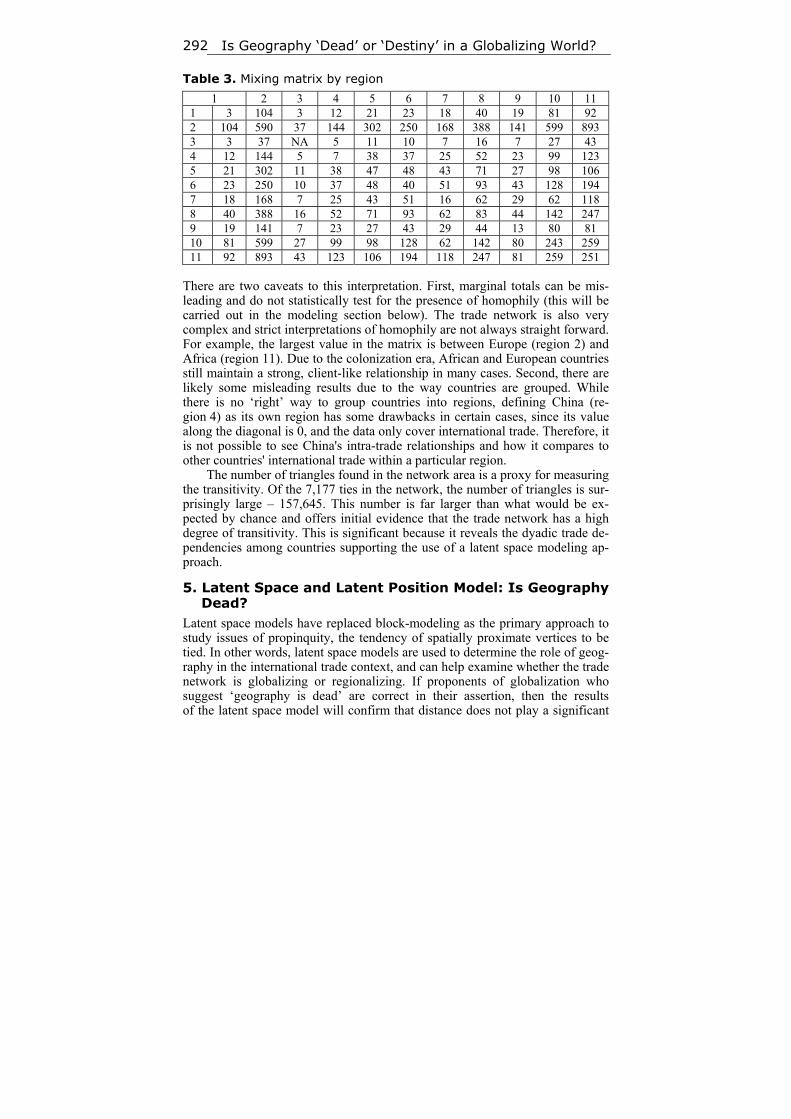
Is Geography ‘Dead’ or ‘Destiny’ in a Globalizing World? 292
Table 3. Mixing matrix by region
1 2 3 4 5 6 7 8 9 10 11 1 3 104 3 12 21 23 18 40 19 81 92 2 104 590 37 144 302 250 168 388 141 599 893 3 3 37 NA 5 11 10 7 16 7 27 43 4 12 144 5 7 38 37 25 52 23 99 123 5 21 302 11 38 47 48 43 71 27 98 106 6 23 250 10 37 48 40 51 93 43 128 194 7 18 168 7 25 43 51 16 62 29 62 118 8 40 388 16 52 71 93 62 83 44 142 247 9 19 141 7 23 27 43 29 44 13 80 81 10 81 599 27 99 98 128 62 142 80 243 259 11 92 893 43 123 106 194 118 247 81 259 251
There are two caveats to this interpretation. First, marginal totals can be mis-leading and do not statistically test for the presence of homophily (this will be carried out in the modeling section below). The trade network is also very complex and strict interpretations of homophily are not always straight forward. For example, the largest value in the matrix is between Europe (region 2) and Africa (region 11). Due to the colonization era, African and European countries still maintain a strong, client-like relationship in many cases. Second, there are likely some misleading results due to the way countries are grouped. While there is no ‘right’ way to group countries into regions, defining China (re-gion 4) as its own region has some drawbacks in certain cases, since its value along the diagonal is 0, and the data only cover international trade. Therefore, it is not possible to see China's intra-trade relationships and how it compares to other countries' international trade within a particular region.
The number of triangles found in the network area is a proxy for measuring the transitivity. Of the 7,177 ties in the network, the number of triangles is sur-prisingly large – 157,645. This number is far larger than what would be ex-pected by chance and offers initial evidence that the trade network has a high degree of transitivity. This is significant because it reveals the dyadic trade de-pendencies among countries supporting the use of a latent space modeling ap-proach.
5. Latent Space and Latent Position Model: Is Geography Dead?
Latent space models have replaced block-modeling as the primary approach to study issues of propinquity, the tendency of spatially proximate vertices to be tied. In other words, latent space models are used to determine the role of geog-raphy in the international trade context, and can help examine whether the trade network is globalizing or regionalizing. If proponents of globalization who suggest ‘geography is dead’ are correct in their assertion, then the results of the latent space model will confirm that distance does not play a significant
Anthony Howell 293
role in influencing the probability that a trade tie is established between country i and country j.
In order to test the role of geography in determining the probability two countries (i, j) form a trade relationship, I specify several latent space models. Based on the presence of homophily indicated by the descriptive statistics, there is evidence that propinquity – the probability of a link between two actors is a function of the distance between them in an unobserved latent space – ex-ists in the trade network.
The latent position model assumes a conditional independence approach to modeling. Let {zi} be the positions of the actors in the social space Rk and {xi, j} denote the observed characteristics that are dyad-specific. That is the presence or absence of a trade tie between two countries is independent of all other ties in the system, given the unobserved positions in social space of the two indi-viduals:
P(Y|Z, X, θ) = P(yi, j | zi, zj, xi, θ), (Eq. 7) where X and xi and xi, j are observed characteristics that are pair-specific and vector-valued and θ and Z are parameters and positions to be estimated (Hoff et al. 2002). I use logistic regression to parameterize Eq. 3.
,,,,1log ,,, jijijiji xzzyodds . (Eq. 8)
jijiji zzx ,, , (Eq. 9)
where the log odds ratio for two actors j and k, equidistant from i, is
kiji xxB ,,, . I estimate i, j using the log-likelihood of a conditional independ-
ence model, expressed as
ji
jijijieyYP ,1loglog ,,
, (Eq. 10)
where is a function of parameters and unknown positions. As such, I use maximum-likelihood to estimate . Model degeneracy is a serious problem that frequently occurs when dealing with networks. If a model is degenerate then the terms in the model are grossly unsuitable at describing the underlying proc-esses that form the observed network. That is, even under the maximum likeli-hood coefficients in the model, the observed network is so unlikely to occur that the model cannot even be properly estimated (Goodreau et al. 2008). To check for issues of degeneracy, I carry out an MCMC estimation procedure for each model that I estimate. The results show that the model statistics do not diverge from the mean, meaning that the models are not degenerate and the maximum likelihood estimates are reliable.
I specify several simple latent space models to test the role of distance and region-based homophily. Table 4 reports the coefficients generated from the latent space models. Model 1 only examines the role of distance in establishing a trade partner. The coefficient on EDGES is highly significant and positive, indicating that larger distances increase the likelihood of two countries estab-
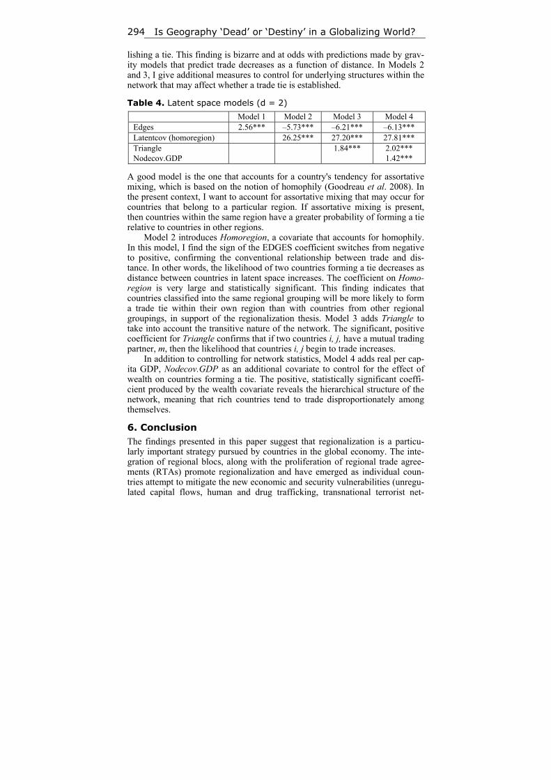
Is Geography ‘Dead’ or ‘Destiny’ in a Globalizing World? 294
lishing a tie. This finding is bizarre and at odds with predictions made by grav-ity models that predict trade decreases as a function of distance. In Models 2 and 3, I give additional measures to control for underlying structures within the network that may affect whether a trade tie is established.
Table 4. Latent space models (d = 2)
Model 1 Model 2 Model 3 Model 4 Edges 2.56*** –5.73*** –6.21*** –6.13*** Latentcov (homoregion) 26.25*** 27.20*** 27.81*** Triangle Nodecov.GDP
1.84*** 2.02*** 1.42***
A good model is the one that accounts for a country's tendency for assortative mixing, which is based on the notion of homophily (Goodreau et al. 2008). In the present context, I want to account for assortative mixing that may occur for countries that belong to a particular region. If assortative mixing is present, then countries within the same region have a greater probability of forming a tie relative to countries in other regions.
Model 2 introduces Homoregion, a covariate that accounts for homophily. In this model, I find the sign of the EDGES coefficient switches from negative to positive, confirming the conventional relationship between trade and dis-tance. In other words, the likelihood of two countries forming a tie decreases as distance between countries in latent space increases. The coefficient on Homo-region is very large and statistically significant. This finding indicates that countries classified into the same regional grouping will be more likely to form a trade tie within their own region than with countries from other regional groupings, in support of the regionalization thesis. Model 3 adds Triangle to take into account the transitive nature of the network. The significant, positive coefficient for Triangle confirms that if two countries i, j, have a mutual trading partner, m, then the likelihood that countries i, j begin to trade increases.
In addition to controlling for network statistics, Model 4 adds real per cap-ita GDP, Nodecov.GDP as an additional covariate to control for the effect of wealth on countries forming a tie. The positive, statistically significant coeffi-cient produced by the wealth covariate reveals the hierarchical structure of the network, meaning that rich countries tend to trade disproportionately among themselves.
6. Conclusion The findings presented in this paper suggest that regionalization is a particu-larly important strategy pursued by countries in the global economy. The inte-gration of regional blocs, along with the proliferation of regional trade agree-ments (RTAs) promote regionalization and have emerged as individual coun-tries attempt to mitigate the new economic and security vulnerabilities (unregu-lated capital flows, human and drug trafficking, transnational terrorist net-
Anthony Howell 295
works, disease, etc.) brought about by globalizing forces that undermine indi-vidual states' territorial sovereignty. The process of regionalization signals that ‘geography is destiny’ (Dieter 2007: 11), as opposed to ‘geography is dead’.
The results of the descriptive analyses in this report agree with other previ-ous works. The WTN network has a high density, the node degree has a high right-skew, trade partners of well-connected countries are less interconnected relative to those of poorly connected ones, and countries holding many trade partners are on average connected with countries holding relatively few coun-tries. The latent space model tests directly the role of space in determining the likelihood of whether or not a tie will be established. When controlling for re-gional homophily and other covariates, the Euclidean distance – calculated in social space – is returned negative, significant, and large in magnitude. This result supports findings in the gravitas literature on trade and reaffirms that the probability that trade ties are established decreases as distance increases. Last-ly, the latent space models add an additional dimension of analysis of the WTN by controlling for network dependencies, and reveals that region-based homo-phily – the proxy for regionalization – has a large and significant influence on trade outcomes, even more so than a country's wealth.
Despite the complicated nature of the WTN, pertinent topological proper-ties of the global trade system are extracted through modeling the system as a network, and are used to show the significance of geography in influencing trade outcomes. Understanding the structure of the global trade network has implications for research across numerous social science disciplines trying to examine the effects of geography on economic integration and internationaliza-tion. Future areas of research can extend the latent space model applied in this paper to examine the evolutionary role of geography over time. Although evi-dence reported in this paper suggests that geography maintains a crucial role in the trade network, it is indeterminate whether geography's impact on trade ties is increasing or decreasing over time.
References
Aggarwal V. K., and Koo M. G. 2005. Beyond Network Power? The Dynamics of Formal Economic Integration in Northeast Asia. The Pacific Review 18: 189–216.
Bhagwati J., Greenaway D., and Panagariya A. 1999. Trading Preferentially: Theory and Policy. The Economic Journal 108: 1128–1148.
Bhattacharya K., Mukherjee G., Saramaki J., Kaski K., and Manna S. 2008. The International Trade Network: Weighted Network Analysis and Modeling. Jour-nal of Statistical Mechanics: Theory and Experiment 2008(02): P02002. Doi:10.1088/1742-5468/2008/02/p02002.
Clark R. 2008. Dependency, Network Integration, and Development. Sociological Per-spectives 51: 629–648.
Clark R. 2010. World-System Mobility and Economic Growth, 1980–2000. Social Forces 88: 1123–1151.
Is Geography ‘Dead’ or ‘Destiny’ in a Globalizing World? 296
Dieter H. 2007. An Introduction. The Evolution of Regionalism in Asia: Economic and Security Issues / Ed. by H. Dieter, pp. 3–10. London: Routledge.
Fagiolo G., Reyes J., and Schiavo S. 2009. World-Trade Web: Topological Properties, Dynamics, and Evolution. Physical Review E Statistical 79: 1–36.
Friedmann J. 1995. Where We Stand: A Decade of World City Research. World Cities in a World-System / Ed. by P. Knox and P. Taylor, pp. 21–47. Cambridge: Cambridge University Press.
Garlaschelli D., and Loffredo M. 2005. Structure and Evolution of the World Trade Network. Physica A: Statistical Mechanics and Its Applications 355: 138–144.
Garlaschelli D., Di Matteo T., Aste T., Caldarelli G., and Loffredo M. 2007. Inter-play between Topology and Dynamics in the World Trade Web. The European Physical Journal B 57: 159–164.
Goodreau S. M., Handcock M. S., Hunter D. R., Butts C. T., and Morris M. 2008. A Statnet Tutorial. Journal of Statistical Software 24: 1–27.
Harary F. 1959. A Graph Theoretic Method for the Complete Reduction of a Matrix with a View Toward Finding its Eigenvalues. Journal of Math Physics 68: 104–111.
Harary F., Norman R., and Cartwright D. 1965. Structural Models: An Introduction to the Theory of Directed Graphs. New York: Wiley.
He J., and Deem M. 2010. Structure and Response in the World Trade Network. Physi-cal Review Letters 105: 1–4.
Hoff P. D., Raftery A. E., and Handcock M. S. 2002. Latent Space Approaches to Social Network Analysis. Journal of the American Statistical Association 9: 1090–1098.
Hunter D. R., and Handcock M. S. 2005. Inference in Curved Exponential Family Models for Networks. Journal of Computational and Graphical Statistics 15: 565–583.
Kali R., and Reyes J. 2007. The Architecture of Globalization: A Network Approach to International Economic Integration. Journal of International Business Studies 38: 595–620.
Kastelle T., Steen J., and Liesch P. 2006. Measuring Globalization: An Evolutionary Economic Approach to Tracking the Evolution of International Trade. DRUID Summer Conference, рр. 1–41. Copenhagen.
Kim S., and Shin E.-H. 2002. A Longitudinal Analysis of Globalization and Regionalization in International Trade: A Social Network Approach. Social Forces 81: 445–468.
Krivitsky P. N., Handcock M. S., Raftery A. E., and Hoff P. D. 2009. Representing Degree Distributions Clustering and Homophily in Social Networks with Latent Cluster Random Effects Models. Social Networks 31: 204–213.
Krugman P. 1993. Geography and Trade. Cambridge, MA: Cambridge University Press.
Louch H. 2000. Personal Network Integration: Transitivity and Homophily in Strong-Tie Relations. Social Networks 22: 45–64.
Massey D. 1984. Spatial Divisions of Labor: Social Structures and the Geography of Production. New York: Methuen.
Massey D. 1999. Imagining Globalization: Power-Geometries of Time-Space. Global Futures: Migration Environment and Globalization / Ed. by A. Brah, M. Hickman, and M. Mac an Ghaill, pp. 27–44. Basingstoke: Macmillan.
Anthony Howell 297
McPherson M., Smith-Lovin L., and Cook J. M. 2001. Birds of a Feather: Homophily in Social Networks. Annual Review of Sociology 27: 415–444.
Moore T. 2007. China's Rise in Asia: Regional Cooperation and Grand Strategy. Evolu-tion of Regionalism in Asia: Economic and Security Issues / Ed. by H. Dieter, pp. 34–56. London: Routledge.
Morgan K. 2004. The Exaggerated Death of Geography: Learning Proximity and Terri-torial Innovation Systems. Journal of Economic Geography 4: 3–21.
Morris M., Handcock M. S., and Hunter D. R. 2008. Specification of Exponential-Family Random Graph Models: Terms and Computational Aspects. Journal of Sta-tistical Software 24: 1548–7660.
Ohmae K. 1990. The Borderless World: Power and Strategy in the Interlinked Econ-omy. New York: Harper.
Ohmae K. 1995. The Evolving Global Economy: Making Sense of the New World Or-der. Boston, MA: Harvard Business Review Press.
O'Brien R. 1992. Global Financial Integration: The End of Geography. New York: Foreign Relations Press.
Reyes J., Schiavo S., and Fagiolo G. 2007. Using Complex Network Analysis to Assess the Evolution of International Economic Integration: The Cases of East Asia and Latin America. LEM Working Paper Series, No 25. Pisa: Laboratory of Economics and Management, Sant' Anna School of Advanced Studies.
Reyes J., Schiavo S., and Fagiolo G. 2010. Using Complex Networks Analysis to As-sess the Evolution of International Economic Integration: The Cases of East Asia and Latin America. The Journal of International Trade & Economic Development 19: 215–239.
Schiavo S., Reyes J., and Fagiolo G. 2010. International Trade and Financial Integra-tion: A Weighted Network Analysis. Quantitative Finance 10: 389–399.
Serrano M. 2008. Rich-Club vs Rich-Multipolarization Phenomena in Weighted Net-works. Physical Review E 78: 026101.
Serrano M. A., and Boguna M. 2003. Topology of the World Trade Web. Physical Review E 68: 015101.
Shortreed S., Handcock M. S., and Hoff P. D. 2006. Positional Estimation within the Latent Space Model for Networks. Methodology 2: 24–33.
Squartini T., Fagiolo G., and Garlaschelli D. 2011. Rewiring World Trade. Part I. A Binary Network Analysis. LEM Working Paper Series, No 8. Pisa: Laboratory of Economics and Management, Sant' Anna School of Advanced Studies. URL: http://www.lem.sssup.it/wplem.html.
Staples A. 2007. Responses to Regionalism: Corporate Strategy in East Asia. Evolution of Regionalism in Asia: Economic and Security Issues / Ed. by H. Dieter, pp. 99–122. London: Routledge.
Toffler A. 1970. Future Shock. New York: Bantam Books.
Warwick M. 2005. Geographies of Globalization. London – New York: Routledge.
Yeung H. 1998. Capital State and Space: Contesting the Borderless World. Transac-tions of the Institute of Brittish Geographers 23: 291–309.
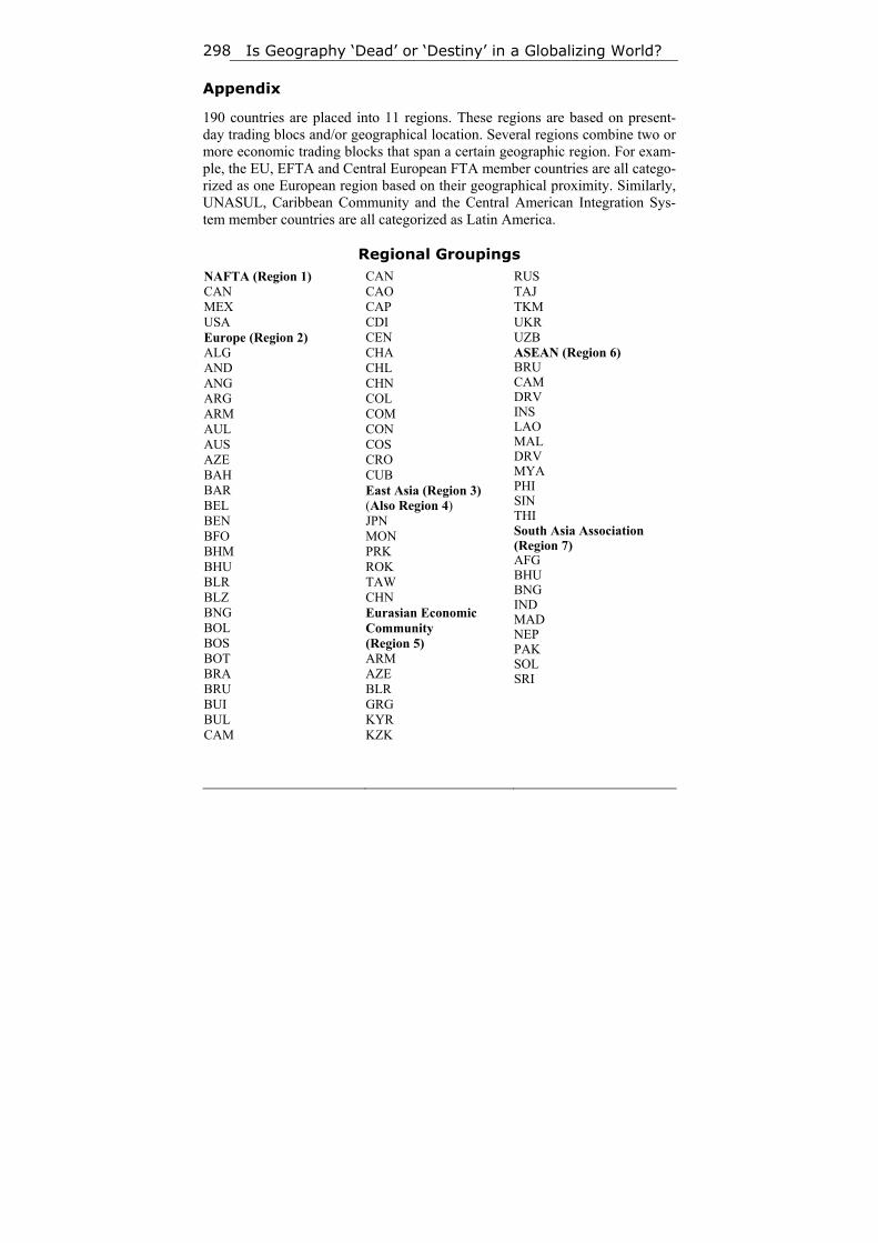
Is Geography ‘Dead’ or ‘Destiny’ in a Globalizing World? 298
Appendix
190 countries are placed into 11 regions. These regions are based on present-day trading blocs and/or geographical location. Several regions combine two or more economic trading blocks that span a certain geographic region. For exam-ple, the EU, EFTA and Central European FTA member countries are all catego-rized as one European region based on their geographical proximity. Similarly, UNASUL, Caribbean Community and the Central American Integration Sys-tem member countries are all categorized as Latin America.
Regional Groupings NAFTA (Region 1) CAN MEX USA Europe (Region 2) ALG AND ANG ARG ARM AUL AUS AZE BAH BAR BEL BEN BFO BHM BHU BLR BLZ BNG BOL BOS BOT BRA BRU BUI BUL CAM
CAN CAO CAP CDI CEN CHA CHL CHN COL COM CON COS CRO CUB East Asia (Region 3) (Also Region 4) JPN MON PRK ROK TAW CHN Eurasian Economic Community (Region 5) ARM AZE BLR GRG KYR KZK
RUS TAJ TKM UKR UZB ASEAN (Region 6) BRU CAM DRV INS LAO MAL DRV MYA PHI SIN THI South Asia Association (Region 7) AFG BHU BNG IND MAD NEP PAK SOL SRI
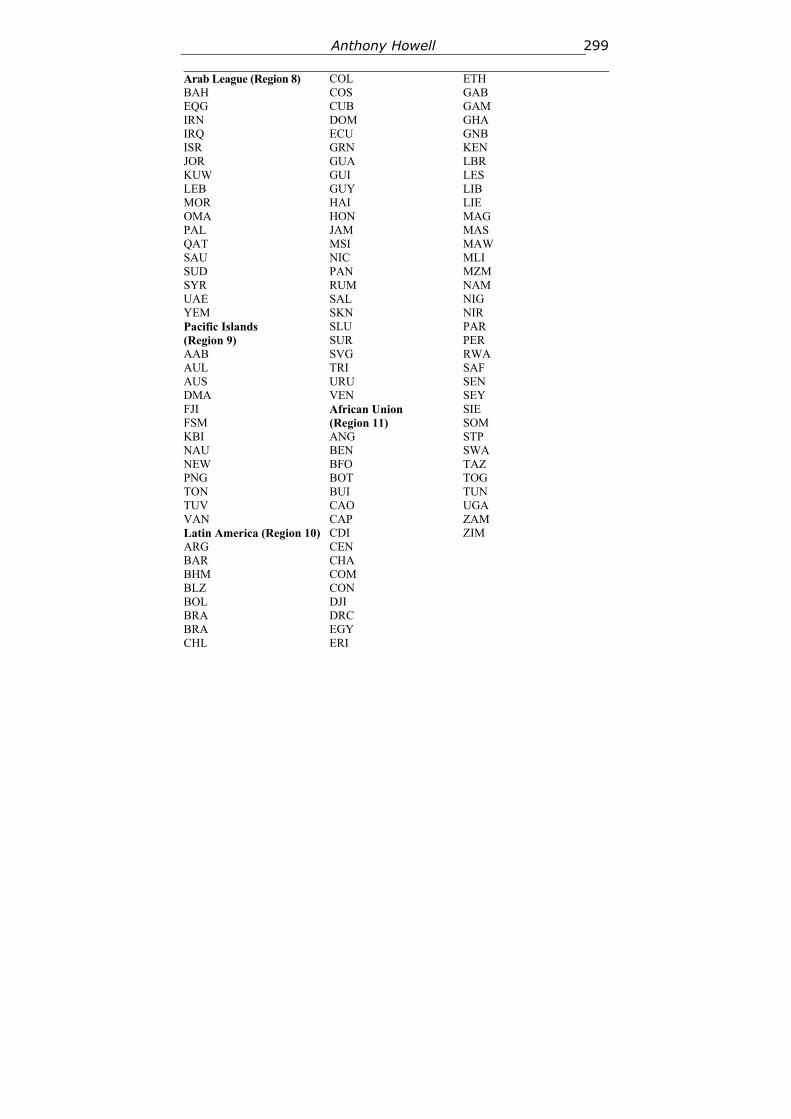
Anthony Howell 299
Arab League (Region 8) BAH EQG IRN IRQ ISR JOR KUW LEB MOR OMA PAL QAT SAU SUD SYR UAE YEM Pacific Islands (Region 9) AAB AUL AUS DMA FJI FSM KBI NAU NEW PNG TON TUV VAN Latin America (Region 10) ARG BAR BHM BLZ BOL BRA BRA CHL
COL COS CUB DOM ECU GRN GUA GUI GUY HAI HON JAM MSI NIC PAN RUM SAL SKN SLU SUR SVG TRI URU VEN African Union (Region 11) ANG BEN BFO BOT BUI CAO CAP CDI CEN CHA COM CON DJI DRC EGY ERI
ETH GAB GAM GHA GNB KEN LBR LES LIB LIE MAG MAS MAW MLI MZM NAM NIG NIR PAR PER RWA SAF SEN SEY SIE SOM STP SWA TAZ TOG TUN UGA ZAM ZIM
History & Mathematics: Trends and Cycles 2014 300–313
300
10
The British-Italian Performance in the Mediterranean from the Artillery
Perspective
Kent R. Crawford and Nicholas W. Mitiukov
Abstract
The Italian defeat in the Second World War was a consequence of its failure to dominate the central Mediterranean. In the numerous works that address the issue, scholars tend to see reasons of a political nature, shortcomings in the organization and planning by the Italian Navy, indecisive political leader-ship, and so on. But all agree that technically the Italian fleet was superior to British ships deployed in the Mediterranean area, and in this regard the defeat of the Italians is seen as paradoxical. In this paper, the authors explore the theory that the poor showing of the Italian navy may have resulted from the errors of the political, military and technical leadership in the prewar period, in particular in the performance of the Italian naval artillery.
Keywords: Mediterranean history, naval history, Italy, Great Britain, his-torical reconstruction.
Introduction
In recent years the phrase ‘technical innovation’ has been widely used in the literature or for various purposes. But nevertheless, there is an undeniable con-nection between social evolution and technical innovation. Probably, one can find the most original presentation of this relationship in Theory of Cultural Circles by Fritz Graebner (Methode der Ethnologie; see Graebner 1911). When analyzing ancient and medieval data, it is easy to notice that progress in techni-cal areas, especially in military technology, could give the possessors of these innovations a decisive advantage over other nations, contribute to the conquest and exploration of new territories, and insure a certain domestic tranquility. Also there is no doubt that the level of innovation is ‘cumulative’; each subse-quent military innovation is much more effective than the previous one. Nor is there any doubt that a continual innovation became the key to survival. For instance, in the twelfth century, Saladin's Moslems perfected the horse archer regarding it as the ultimate weapon. Thereafter, the innovation in the military
Kent R. Crawford and Nicholas W. Mitiukov 301
sphere virtually ceased, and the Muslim states thus missed out on the develop-ments in gunpowder weapons.
The twentieth-century data brought about some changes in this coherent theory. It turned out that the nature of technical innovations varies, which is most clearly demonstrated by the evolution of naval artillery. Because of the high cost, hardly anyone, even the richest state, could afford to evolve artillery by trial and error or aesthetics, but had to develop and strictly adhere to a cer-tain doctrine, referred to in the literature as ‘technology policy’. For example, advances in development of propellant powders and artillery materiel in the beginning of the twentieth century was applied to create a new generation of artillery for high muzzle velocities and therefore, better ballistic performance. And it became possible to design artillery with the performance of the previous generation, but much easier and simpler to produce, and hence less expensive. In this case, there seems to be a continuing conformity with the ‘cultural cir-cles’, though this is an illusion. It was just the high cost and complexity of the twentieth-century artillery technology that turned out to be a trap in innovation. If the underlying facts and theories for a particular technology policy decision subsequently prove to have been incorrect, the resulting material must still be used until it can be replaced, with corresponding performance issues. Making a wrong choice in policy has serious and costly consequences.
To illustrate the effect of such a highly subjective characteristic as ‘tech-nology policy’ at the macro-level, one needs merely to look at the combat op-erations in the Mediterranean theater of the Second World War. The most char-acteristic feature are the operation in 1940–1943, the period of active participa-tion in the war at sea in Italy. In the late 1920s and 1930s, Italy had been virtu-ally isolated from the influence of external military innovation, primarily Ger-man and American. And in point of fact, the Italian ordnance technology had its origins in the British firms such as Armstrong/Elswick and Vickers in the late nineteenth century, which continued through and immediately following the Great War, after which the source ‘dried up’ and left the Italians to their own devices. So, in a general sense, their ordnance of the Second World War pre-dominately reflected the Italian policy decisions.
Perhaps, more than any other form of combat, naval warfare is dominated by technology. For example, the naval engagements of the Russo-Japanese War (1904–1905) may be viewed in terms of French and French influenced technol-ogy versus British technology. In a like manner, the combat in the 1940–1943 period compares the products of Italian versus British technology. At stake was control of the central Mediterranean, necessary to provide the ability to supply and reinforce the military forces in North Africa.
Historical Note
The naval war in the Mediterranean Sea from 1940 to 1943 is still the subject of much controversy, revolved not so much about what actually happened, but
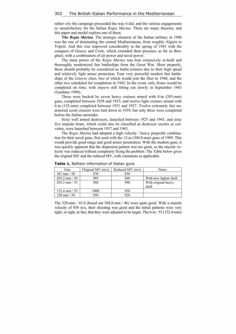
The British-Italian Performance in the Mediterranean 302
rather why the campaign proceeded the way it did, and the various engagements so unsatisfactory for the Italian Regia Marina. There are many theories, and this paper and model explore one of them.
The Regia Marina. The strategic situation of the Italian military in 1940 was the one of dominating the central Mediterranean, from roughly Algiers to Tripoli. And this was improved considerably in the spring of 1941 with the conquest of Greece and Crete, which extended their presence as far as Ben-ghazi, with a combination of air power and naval power.
The main power of the Regia Marina was four extensively re-built and thoroughly modernized fast battleships from the Great War. More properly, these should probably be considered as battle-cruisers due to their high speed and relatively light armor protection. Four very powerful modern fast battle-ships of the Littorio class, two of which would join the fleet in 1940, and the other two scheduled for completion in 1942. In the event, only Roma would be completed on time, with Impero still fitting out slowly in September 1943 (Gardiner 1980).
These were backed by seven heavy cruisers armed with 8-in (203-mm) guns, completed between 1928 and 1933, and twelve light cruisers armed with 6-in (152-mm) completed between 1931 and 1937. Twelve extremely fast un-armored scout cruisers were laid down in 1939, but only three were completed before the Italian surrender.
Sixty well armed destroyers, launched between 1925 and 1943, and sixty five torpedo boats, which could also be classified as destroyer escorts or cor-vettes, were launched between 1937 and 1943.
The Regia Marina had adopted a high velocity / heavy projectile combina-tion for their naval guns, first used with the 12-in (304.8-mm) guns of 1909. This would provide good range and good armor penetration. With the modern guns, it was quickly apparent that the dispersion pattern was too great, so the muzzle ve-locity was reduced without completely fixing the problem. The Table below gives the original MV and the reduced MV, with comments as applicable.
Table 1. Ballistic information of Italian guns
Gun Original MV (m/s) Reduced MV (m/s) Notes 381 mm / 50 870 850 203.2 mm / 50 905 840 With new lighter shell 203.2 mm / 53 960 900 With original heavy
shell 152.4 mm / 53 1000 850 120 mm / 50 950 920
The 320-mm / 43.8 (bored out 304.8-mm / 46) were quite good. With a muzzle velocity of 830 m/s, their shooting was good and the initial patterns were very tight; so tight, in fact, that they were adjusted to be larger. The 6-in / 55 (152.4-mm)
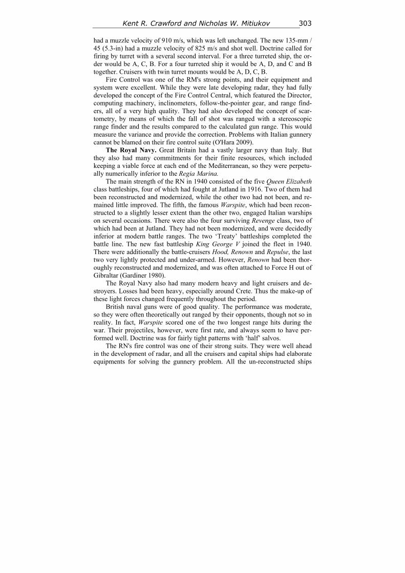
Kent R. Crawford and Nicholas W. Mitiukov 303
had a muzzle velocity of 910 m/s, which was left unchanged. The new 135-mm / 45 (5.3-in) had a muzzle velocity of 825 m/s and shot well. Doctrine called for firing by turret with a several second interval. For a three turreted ship, the or-der would be A, C, B. For a four turreted ship it would be A, D, and C and B together. Cruisers with twin turret mounts would be A, D, C, B.
Fire Control was one of the RM's strong points, and their equipment and system were excellent. While they were late developing radar, they had fully developed the concept of the Fire Control Central, which featured the Director, computing machinery, inclinometers, follow-the-pointer gear, and range find-ers, all of a very high quality. They had also developed the concept of scar-tometry, by means of which the fall of shot was ranged with a stereoscopic range finder and the results compared to the calculated gun range. This would measure the variance and provide the correction. Problems with Italian gunnery cannot be blamed on their fire control suite (O'Hara 2009).
The Royal Navy. Great Britain had a vastly larger navy than Italy. But they also had many commitments for their finite resources, which included keeping a viable force at each end of the Mediterranean, so they were perpetu-ally numerically inferior to the Regia Marina.
The main strength of the RN in 1940 consisted of the five Queen Elizabeth class battleships, four of which had fought at Jutland in 1916. Two of them had been reconstructed and modernized, while the other two had not been, and re-mained little improved. The fifth, the famous Warspite, which had been recon-structed to a slightly lesser extent than the other two, engaged Italian warships on several occasions. There were also the four surviving Revenge class, two of which had been at Jutland. They had not been modernized, and were decidedly inferior at modern battle ranges. The two ‘Treaty’ battleships completed the battle line. The new fast battleship King George V joined the fleet in 1940. There were additionally the battle-cruisers Hood, Renown and Repulse, the last two very lightly protected and under-armed. However, Renown had been thor-oughly reconstructed and modernized, and was often attached to Force H out of Gibraltar (Gardiner 1980).
The Royal Navy also had many modern heavy and light cruisers and de-stroyers. Losses had been heavy, especially around Crete. Thus the make-up of these light forces changed frequently throughout the period.
British naval guns were of good quality. The performance was moderate, so they were often theoretically out ranged by their opponents, though not so in reality. In fact, Warspite scored one of the two longest range hits during the war. Their projectiles, however, were first rate, and always seem to have per-formed well. Doctrine was for fairly tight patterns with ‘half’ salvos.
The RN's fire control was one of their strong suits. They were well ahead in the development of radar, and all the cruisers and capital ships had elaborate equipments for solving the gunnery problem. All the un-reconstructed ships
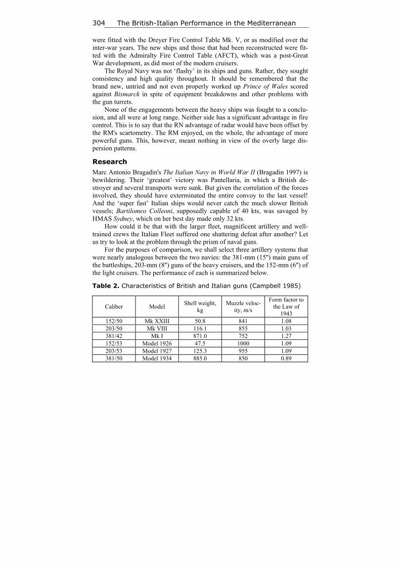
The British-Italian Performance in the Mediterranean 304
were fitted with the Dreyer Fire Control Table Mk. V, or as modified over the inter-war years. The new ships and those that had been reconstructed were fit-ted with the Admiralty Fire Control Table (AFCT), which was a post-Great War development, as did most of the modern cruisers.
The Royal Navy was not ‘flashy’ in its ships and guns. Rather, they sought consistency and high quality throughout. It should be remembered that the brand new, untried and not even properly worked up Prince of Wales scored against Bismarck in spite of equipment breakdowns and other problems with the gun turrets.
None of the engagements between the heavy ships was fought to a conclu-sion, and all were at long range. Neither side has a significant advantage in fire control. This is to say that the RN advantage of radar would have been offset by the RM's scartometry. The RM enjoyed, on the whole, the advantage of more powerful guns. This, however, meant nothing in view of the overly large dis-persion patterns.
Research
Marc Antonio Bragadin's The Italian Navy in World War II (Bragadin 1997) is bewildering. Their ‘greatest’ victory was Pantellaria, in which a British de-stroyer and several transports were sunk. But given the correlation of the forces involved, they should have exterminated the entire convoy to the last vessel! And the ‘super fast’ Italian ships would never catch the much slower British vessels; Bartilomeo Colleoni, supposedly capable of 40 kts, was savaged by HMAS Sydney, which on her best day made only 32 kts.
How could it be that with the larger fleet, magnificent artillery and well-trained crews the Italian Fleet suffered one shattering defeat after another? Let us try to look at the problem through the prism of naval guns.
For the purposes of comparison, we shall select three artillery systems that were nearly analogous between the two navies: the 381-mm (15'') main guns of the battleships, 203-mm (8'') guns of the heavy cruisers, and the 152-mm (6'') of the light cruisers. The performance of each is summarized below.
Table 2. Characteristics of British and Italian guns (Campbell 1985)
Caliber Model Shell weight,
kg Muzzle veloc-
ity, m/s
Form factor to the Law of
1943 152/50 Mk XXIII 50.8 841 1.08 203/50 Mk VIII 116.1 855 1.03 381/42 Mk I 871.0 752 1.27 152/53 Model 1926 47.5 1000 1.09 203/53 Model 1927 125.3 955 1.09 381/50 Model 1934 885.0 850 0.89
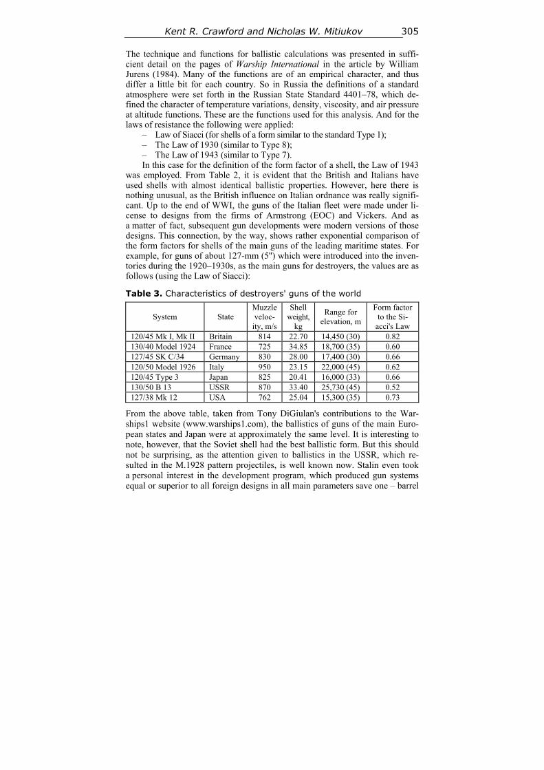
Kent R. Crawford and Nicholas W. Mitiukov 305
The technique and functions for ballistic calculations was presented in suffi-cient detail on the pages of Warship International in the article by William Jurens (1984). Many of the functions are of an empirical character, and thus differ a little bit for each country. So in Russia the definitions of a standard atmosphere were set forth in the Russian State Standard 4401–78, which de-fined the character of temperature variations, density, viscosity, and air pressure at altitude functions. These are the functions used for this analysis. And for the laws of resistance the following were applied:
– Law of Siacci (for shells of a form similar to the standard Type 1); – The Law of 1930 (similar to Type 8); – The Law of 1943 (similar to Type 7). In this case for the definition of the form factor of a shell, the Law of 1943
was employed. From Table 2, it is evident that the British and Italians have used shells with almost identical ballistic properties. However, here there is nothing unusual, as the British influence on Italian ordnance was really signifi-cant. Up to the end of WWI, the guns of the Italian fleet were made under li-cense to designs from the firms of Armstrong (EOC) and Vickers. And as a matter of fact, subsequent gun developments were modern versions of those designs. This connection, by the way, shows rather exponential comparison of the form factors for shells of the main guns of the leading maritime states. For example, for guns of about 127-mm (5'') which were introduced into the inven-tories during the 1920–1930s, as the main guns for destroyers, the values are as follows (using the Law of Siacci):
Table 3. Characteristics of destroyers' guns of the world
System State Muzzle veloc-ity, m/s
Shell weight,
kg
Range for elevation, m
Form factor to the Si-
acci's Law 120/45 Mk I, Mk II Britain 814 22.70 14,450 (30) 0.82 130/40 Model 1924 France 725 34.85 18,700 (35) 0.60 127/45 SK C/34 Germany 830 28.00 17,400 (30) 0.66 120/50 Model 1926 Italy 950 23.15 22,000 (45) 0.62 120/45 Type 3 Japan 825 20.41 16,000 (33) 0.66 130/50 B 13 USSR 870 33.40 25,730 (45) 0.52 127/38 Mk 12 USA 762 25.04 15,300 (35) 0.73
From the above table, taken from Tony DiGiulan's contributions to the War-ships1 website (www.warships1.com), the ballistics of guns of the main Euro-pean states and Japan were at approximately the same level. It is interesting to note, however, that the Soviet shell had the best ballistic form. But this should not be surprising, as the attention given to ballistics in the USSR, which re-sulted in the M.1928 pattern projectiles, is well known now. Stalin even took a personal interest in the development program, which produced gun systems equal or superior to all foreign designs in all main parameters save one – barrel
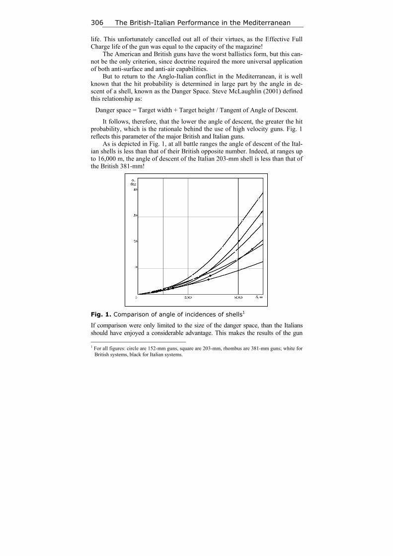
The British-Italian Performance in the Mediterranean 306
life. This unfortunately cancelled out all of their virtues, as the Effective Full Charge life of the gun was equal to the capacity of the magazine!
The American and British guns have the worst ballistics form, but this can-not be the only criterion, since doctrine required the more universal application of both anti-surface and anti-air capabilities.
But to return to the Anglo-Italian conflict in the Mediterranean, it is well known that the hit probability is determined in large part by the angle in de-scent of a shell, known as the Danger Space. Steve McLaughlin (2001) defined this relationship as:
Danger space = Target width + Target height / Tangent of Angle of Descent.
It follows, therefore, that the lower the angle of descent, the greater the hit probability, which is the rationale behind the use of high velocity guns. Fig. 1 reflects this parameter of the major British and Italian guns.
As is depicted in Fig. 1, at all battle ranges the angle of descent of the Ital-ian shells is less than that of their British opposite number. Indeed, at ranges up to 16,000 m, the angle of descent of the Italian 203-mm shell is less than that of the British 381-mm!
Fig. 1. Comparison of angle of incidences of shells1
If comparison were only limited to the size of the danger space, than the Italians should have enjoyed a considerable advantage. This makes the results of the gun 1 For all figures: circle are 152-mm guns, square are 203-mm, rhombus are 381-mm guns; white for
British systems, black for Italian systems.
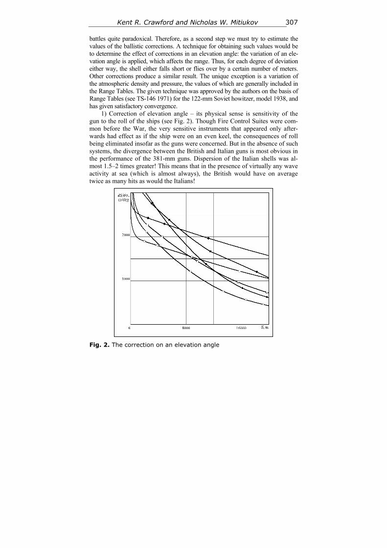
Kent R. Crawford and Nicholas W. Mitiukov 307
battles quite paradoxical. Therefore, as a second step we must try to estimate the values of the ballistic corrections. A technique for obtaining such values would be to determine the effect of corrections in an elevation angle: the variation of an ele-vation angle is applied, which affects the range. Thus, for each degree of deviation either way, the shell either falls short or flies over by a certain number of meters. Other corrections produce a similar result. The unique exception is a variation of the atmospheric density and pressure, the values of which are generally included in the Range Tables. The given technique was approved by the authors on the basis of Range Tables (see TS-146 1971) for the 122-mm Soviet howitzer, model 1938, and has given satisfactory convergence.
1) Correction of elevation angle – its physical sense is sensitivity of the gun to the roll of the ships (see Fig. 2). Though Fire Control Suites were com-mon before the War, the very sensitive instruments that appeared only after-wards had effect as if the ship were on an even keel, the consequences of roll being eliminated insofar as the guns were concerned. But in the absence of such systems, the divergence between the British and Italian guns is most obvious in the performance of the 381-mm guns. Dispersion of the Italian shells was al-most 1.5–2 times greater! This means that in the presence of virtually any wave activity at sea (which is almost always), the British would have on average twice as many hits as would the Italians!
Fig. 2. The correction on an elevation angle
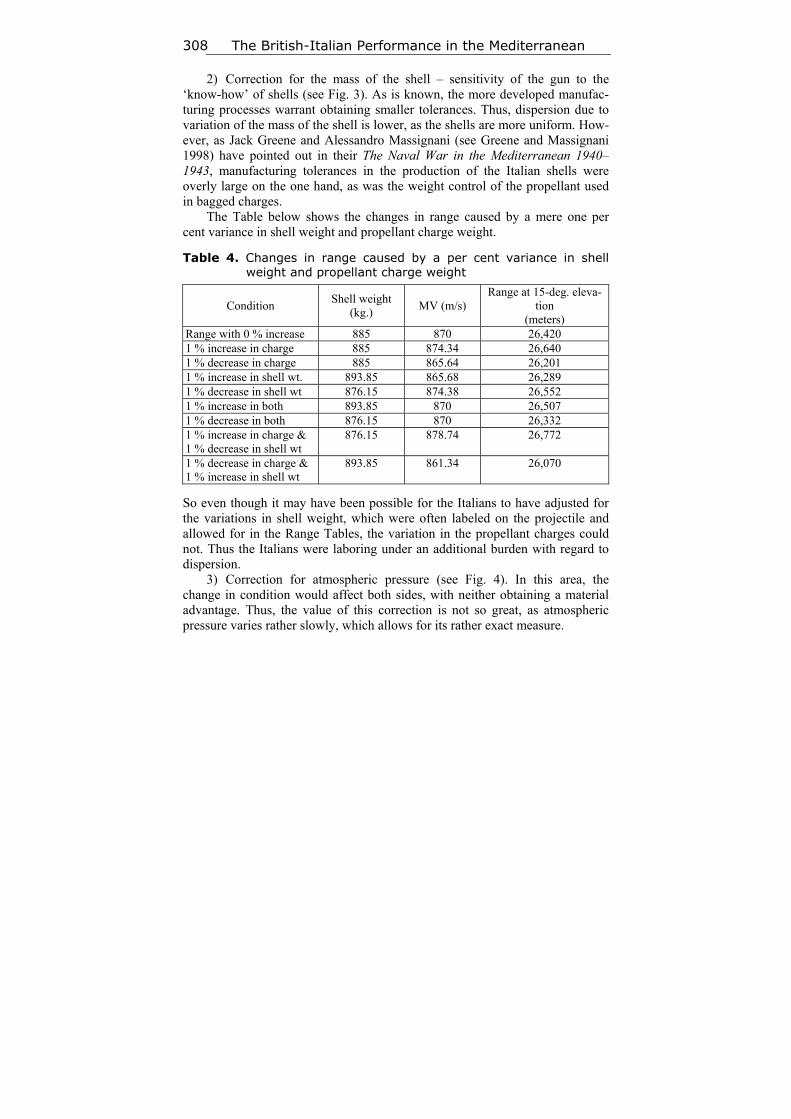
The British-Italian Performance in the Mediterranean 308
2) Correction for the mass of the shell – sensitivity of the gun to the ‘know-how’ of shells (see Fig. 3). As is known, the more developed manufac-turing processes warrant obtaining smaller tolerances. Thus, dispersion due to variation of the mass of the shell is lower, as the shells are more uniform. How-ever, as Jack Greene and Alessandro Massignani (see Greene and Massignani 1998) have pointed out in their The Naval War in the Mediterranean 1940–1943, manufacturing tolerances in the production of the Italian shells were overly large on the one hand, as was the weight control of the propellant used in bagged charges.
The Table below shows the changes in range caused by a mere one per cent variance in shell weight and propellant charge weight.
Table 4. Changes in range caused by a per cent variance in shell weight and propellant charge weight
Condition Shell weight
(kg.) MV (m/s)
Range at 15-deg. eleva-tion
(meters) Range with 0 % increase 885 870 26,420 1 % increase in charge 885 874.34 26,640 1 % decrease in charge 885 865.64 26,201 1 % increase in shell wt. 893.85 865.68 26,289 1 % decrease in shell wt 876.15 874.38 26,552 1 % increase in both 893.85 870 26,507 1 % decrease in both 876.15 870 26,332 1 % increase in charge & 1 % decrease in shell wt
876.15 878.74 26,772
1 % decrease in charge & 1 % increase in shell wt
893.85 861.34 26,070
So even though it may have been possible for the Italians to have adjusted for the variations in shell weight, which were often labeled on the projectile and allowed for in the Range Tables, the variation in the propellant charges could not. Thus the Italians were laboring under an additional burden with regard to dispersion.
3) Correction for atmospheric pressure (see Fig. 4). In this area, the change in condition would affect both sides, with neither obtaining a material advantage. Thus, the value of this correction is not so great, as atmospheric pressure varies rather slowly, which allows for its rather exact measure.
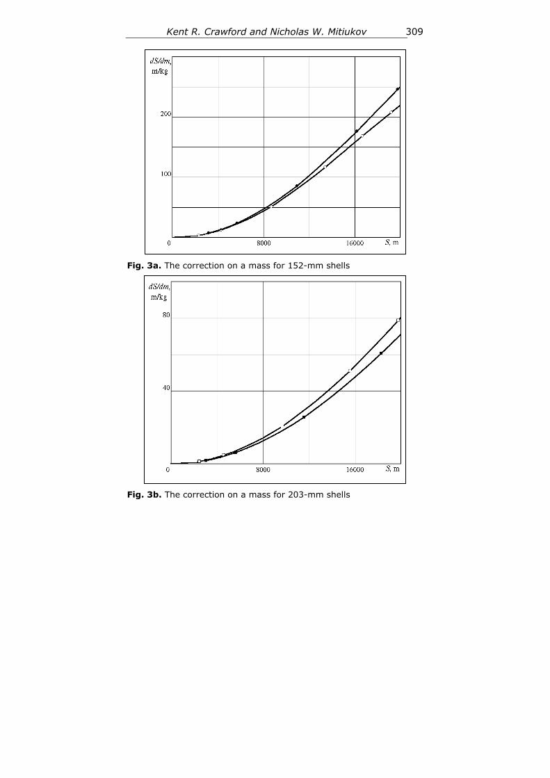
Kent R. Crawford and Nicholas W. Mitiukov 309
Fig. 3a. The correction on a mass for 152-mm shells
Fig. 3b. The correction on a mass for 203-mm shells
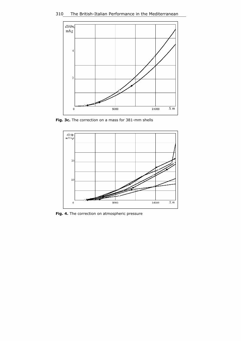
The British-Italian Performance in the Mediterranean 310
Fig. 3c. The correction on a mass for 381-mm shells
Fig. 4. The correction on atmospheric pressure
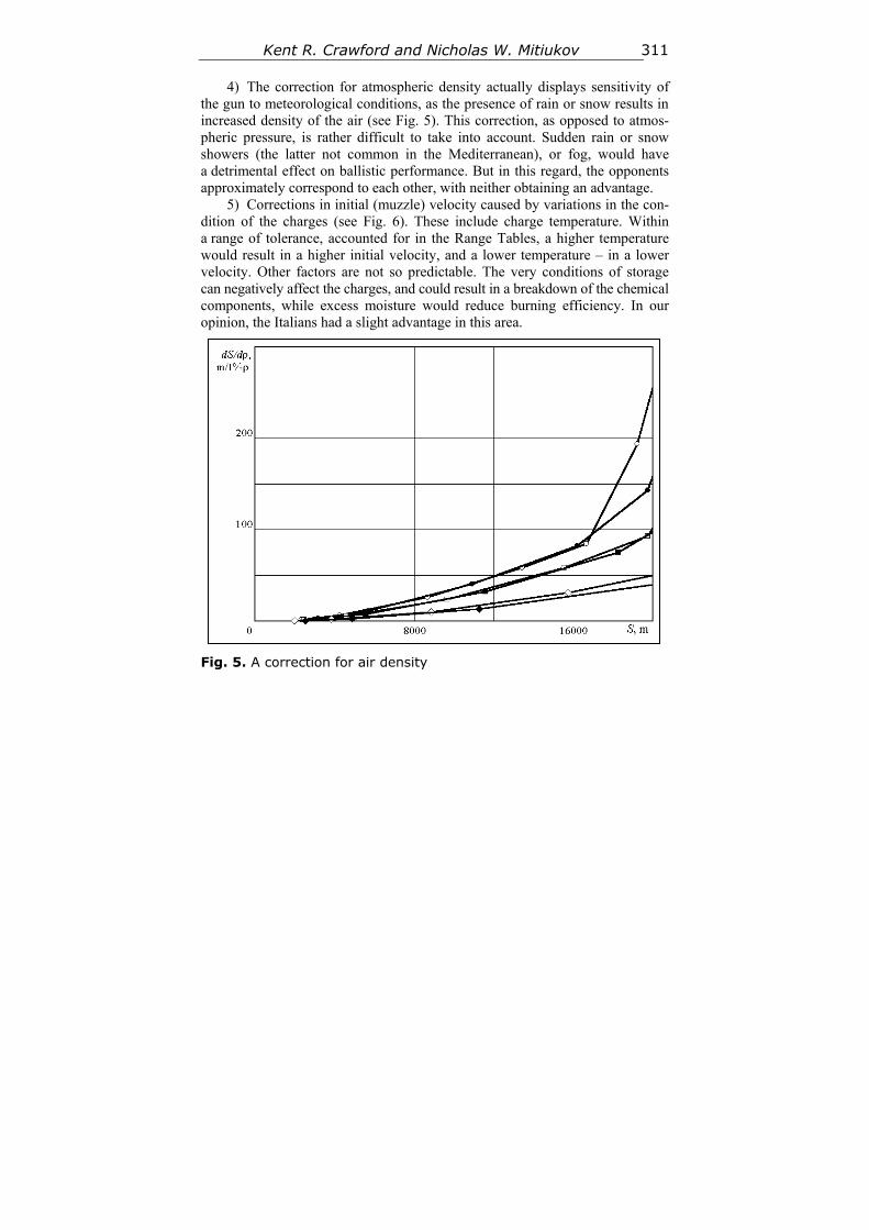
Kent R. Crawford and Nicholas W. Mitiukov 311
4) The correction for atmospheric density actually displays sensitivity of the gun to meteorological conditions, as the presence of rain or snow results in increased density of the air (see Fig. 5). This correction, as opposed to atmos-pheric pressure, is rather difficult to take into account. Sudden rain or snow showers (the latter not common in the Mediterranean), or fog, would have a detrimental effect on ballistic performance. But in this regard, the opponents approximately correspond to each other, with neither obtaining an advantage.
5) Corrections in initial (muzzle) velocity caused by variations in the con-dition of the charges (see Fig. 6). These include charge temperature. Within a range of tolerance, accounted for in the Range Tables, a higher temperature would result in a higher initial velocity, and a lower temperature – in a lower velocity. Other factors are not so predictable. The very conditions of storage can negatively affect the charges, and could result in a breakdown of the chemical components, while excess moisture would reduce burning efficiency. In our opinion, the Italians had a slight advantage in this area.
Fig. 5. A correction for air density
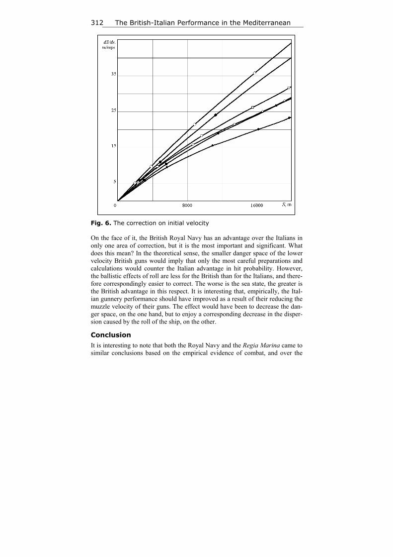
The British-Italian Performance in the Mediterranean 312
Fig. 6. The correction on initial velocity
On the face of it, the British Royal Navy has an advantage over the Italians in only one area of correction, but it is the most important and significant. What does this mean? In the theoretical sense, the smaller danger space of the lower velocity British guns would imply that only the most careful preparations and calculations would counter the Italian advantage in hit probability. However, the ballistic effects of roll are less for the British than for the Italians, and there-fore correspondingly easier to correct. The worse is the sea state, the greater is the British advantage in this respect. It is interesting that, empirically, the Ital-ian gunnery performance should have improved as a result of their reducing the muzzle velocity of their guns. The effect would have been to decrease the dan-ger space, on the one hand, but to enjoy a corresponding decrease in the disper-sion caused by the roll of the ship, on the other.
Conclusion
It is interesting to note that both the Royal Navy and the Regia Marina came to similar conclusions based on the empirical evidence of combat, and over the
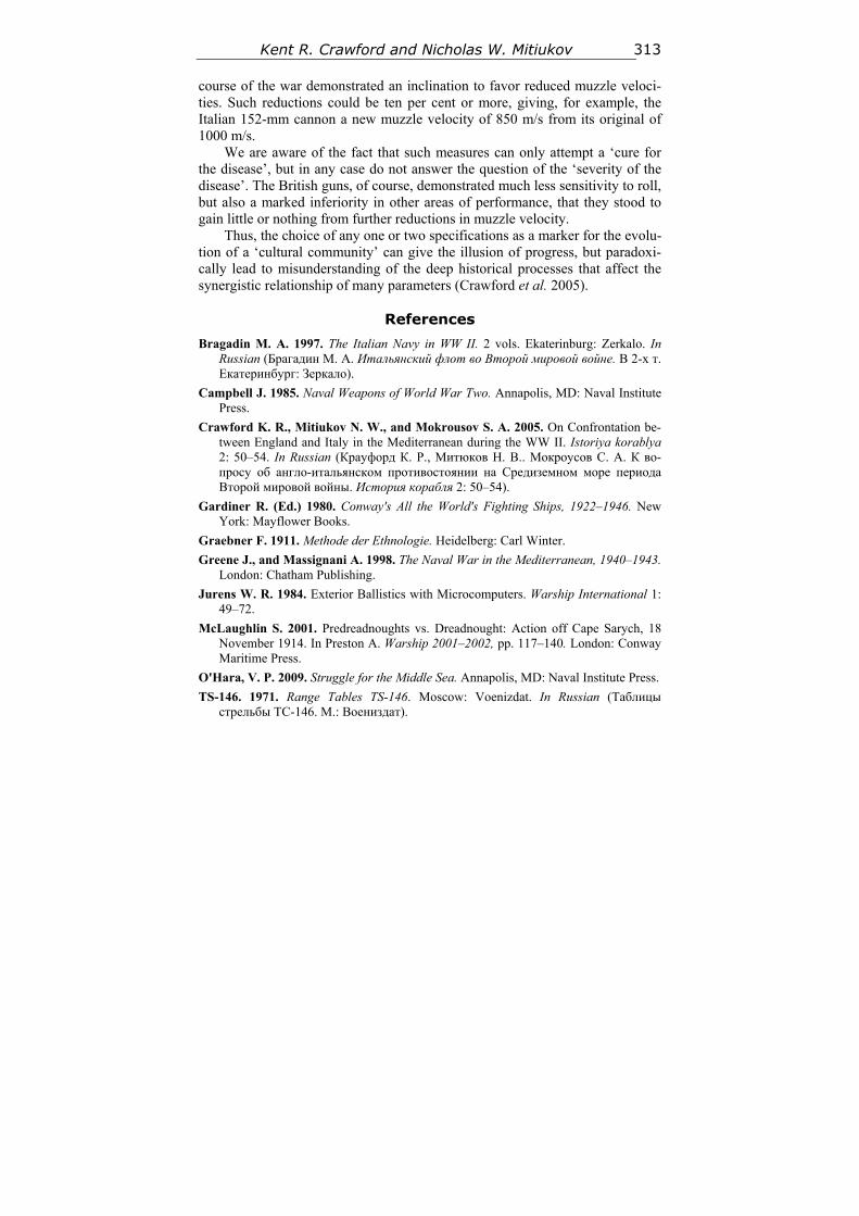
Kent R. Crawford and Nicholas W. Mitiukov 313
course of the war demonstrated an inclination to favor reduced muzzle veloci-ties. Such reductions could be ten per cent or more, giving, for example, the Italian 152-mm cannon a new muzzle velocity of 850 m/s from its original of 1000 m/s.
We are aware of the fact that such measures can only attempt a ‘cure for the disease’, but in any case do not answer the question of the ‘severity of the disease’. The British guns, of course, demonstrated much less sensitivity to roll, but also a marked inferiority in other areas of performance, that they stood to gain little or nothing from further reductions in muzzle velocity.
Thus, the choice of any one or two specifications as a marker for the evolu-tion of a ‘cultural community’ can give the illusion of progress, but paradoxi-cally lead to misunderstanding of the deep historical processes that affect the synergistic relationship of many parameters (Crawford et al. 2005).
References
Bragadin M. A. 1997. The Italian Navy in WW II. 2 vols. Ekaterinburg: Zerkalo. In Russian (Брагадин М. А. Итальянский флот во Второй мировой войне. В 2-х т. Екатеринбург: Зеркало).
Campbell J. 1985. Naval Weapons of World War Two. Annapolis, MD: Naval Institute Press.
Crawford K. R., Mitiukov N. W., and Mokrousov S. A. 2005. On Confrontation be-tween England and Italy in the Mediterranean during the WW II. Istoriya korablya 2: 50–54. In Russian (Крауфорд К. Р., Митюков Н. В.. Мокроусов С. А. К во-просу об англо-итальянском противостоянии на Средиземном море периода Второй мировой войны. История корабля 2: 50–54).
Gardiner R. (Ed.) 1980. Conway's All the World's Fighting Ships, 1922–1946. New York: Mayflower Books.
Graebner F. 1911. Methode der Ethnologie. Heidelberg: Carl Winter.
Greene J., and Massignani A. 1998. The Naval War in the Mediterranean, 1940–1943. London: Chatham Publishing.
Jurens W. R. 1984. Exterior Ballistics with Microcomputers. Warship International 1: 49–72.
McLaughlin S. 2001. Predreadnoughts vs. Dreadnought: Action off Cape Sarych, 18 November 1914. In Preston A. Warship 2001–2002, pp. 117–140. London: Conway Maritime Press.
O'Hara, V. P. 2009. Struggle for the Middle Sea. Annapolis, MD: Naval Institute Press.
ТS-146. 1971. Range Tables TS-146. Moscow: Voenizdat. In Russian (Таблицы стрельбы ТС-146. М.: Воениздат).
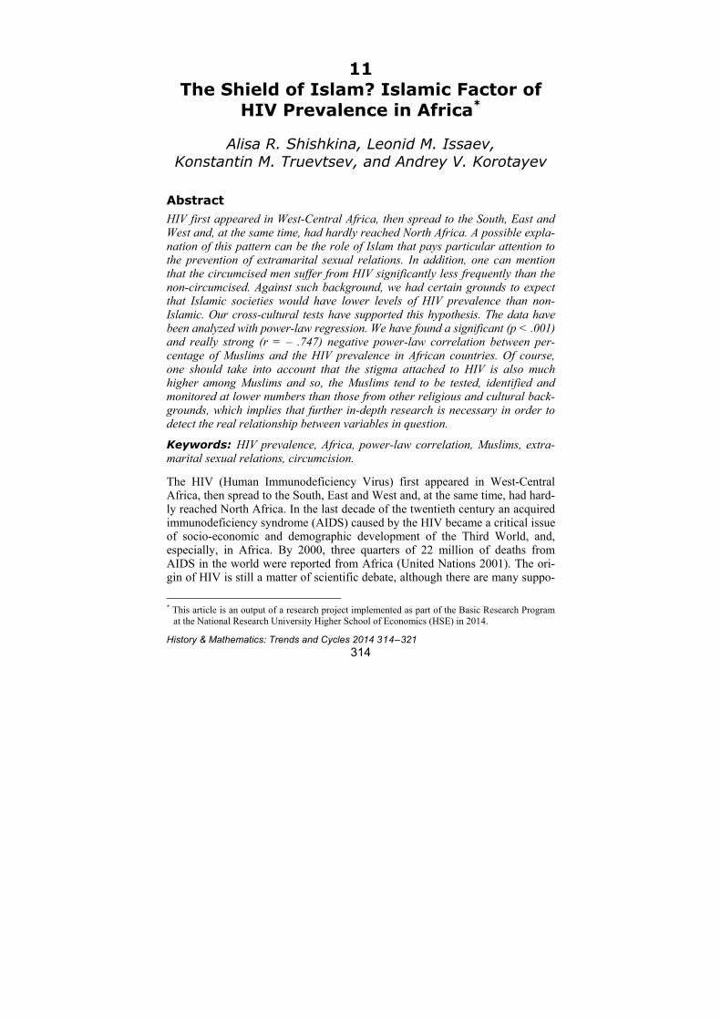
History & Mathematics: Trends and Cycles 2014 314–321
314
11
The Shield of Islam? Islamic Factor of HIV Prevalence in Africa*
Alisa R. Shishkina, Leonid M. Issaev,
Konstantin M. Truevtsev, and Andrey V. Korotayev
Abstract HIV first appeared in West-Central Africa, then spread to the South, East and West and, at the same time, had hardly reached North Africa. A possible expla-nation of this pattern can be the role of Islam that pays particular attention to the prevention of extramarital sexual relations. In addition, one can mention that the circumcised men suffer from HIV significantly less frequently than the non-circumcised. Against such background, we had certain grounds to expect that Islamic societies would have lower levels of HIV prevalence than non-Islamic. Our cross-cultural tests have supported this hypothesis. The data have been analyzed with power-law regression. We have found a significant (p < .001) and really strong (r = – .747) negative power-law correlation between per-centage of Muslims and the HIV prevalence in African countries. Of course, one should take into account that the stigma attached to HIV is also much higher among Muslims and so, the Muslims tend to be tested, identified and monitored at lower numbers than those from other religious and cultural back-grounds, which implies that further in-depth research is necessary in order to detect the real relationship between variables in question.
Keywords: HIV prevalence, Africa, power-law correlation, Muslims, extra-marital sexual relations, circumcision.
The HIV (Human Immunodeficiency Virus) first appeared in West-Central Africa, then spread to the South, East and West and, at the same time, had hard-ly reached North Africa. In the last decade of the twentieth century an acquired immunodeficiency syndrome (AIDS) caused by the HIV became a critical issue of socio-economic and demographic development of the Third World, and, especially, in Africa. By 2000, three quarters of 22 million of deaths from AIDS in the world were reported from Africa (United Nations 2001). The ori-gin of HIV is still a matter of scientific debate, although there are many suppo-
* This article is an output of a research project implemented as part of the Basic Research Program
at the National Research University Higher School of Economics (HSE) in 2014.
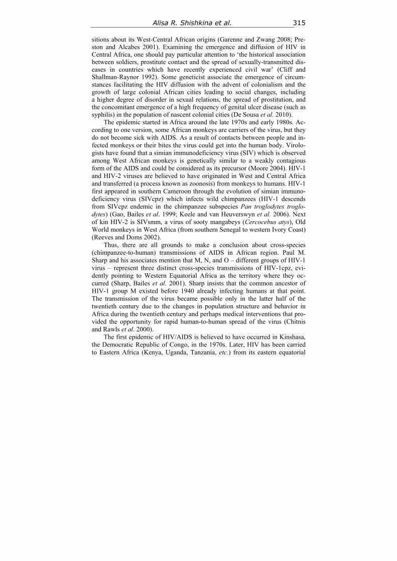
Alisa R. Shishkina et al. 315
sitions about its West-Central African origins (Garenne and Zwang 2008; Pre-ston and Alcabes 2001). Examining the emergence and diffusion of HIV in Central Africa, one should pay particular attention to ‘the historical association between soldiers, prostitute contact and the spread of sexually-transmitted dis-eases in countries which have recently experienced civil war’ (Cliff and Shallman-Raynor 1992). Some geneticist associate the emergence of circum-stances facilitating the HIV diffusion with the advent of colonialism and the growth of large colonial African cities leading to social changes, including a higher degree of disorder in sexual relations, the spread of prostitution, and the concomitant emergence of a high frequency of genital ulcer disease (such as syphilis) in the population of nascent colonial cities (De Sousa et al. 2010).
The epidemic started in Africa around the late 1970s and early 1980s. Ac-cording to one version, some African monkeys are carriers of the virus, but they do not become sick with AIDS. As a result of contacts between people and in-fected monkeys or their bites the virus could get into the human body. Virolo-gists have found that a simian immunodeficiency virus (SIV) which is observed among West African monkeys is genetically similar to a weakly contagious form of the AIDS and could be considered as its precursor (Moore 2004). HIV-1 and HIV-2 viruses are believed to have originated in West and Central Africa and transferred (a process known as zoonosis) from monkeys to humans. HIV-1 first appeared in southern Cameroon through the evolution of simian immuno-deficiency virus (SIVcpz) which infects wild chimpanzees (HIV-1 descends from SIVcpz endemic in the chimpanzee subspecies Pan troglodytes troglo-dytes) (Gao, Bailes et al. 1999; Keele and van Heuverswyn et al. 2006). Next of kin HIV-2 is SIVsmm, a virus of sooty mangabeys (Cercocebus atys), Old World monkeys in West Africa (from southern Senegal to western Ivory Coast) (Reeves and Doms 2002).
Thus, there are all grounds to make a conclusion about cross-species (chimpanzee-to-human) transmissions of AIDS in African region. Paul M. Sharp and his associates mention that M, N, and O – different groups of HIV-1 virus – represent three distinct cross-species transmissions of HIV-1cpz, evi-dently pointing to Western Equatorial Africa as the territory where they oc-curred (Sharp, Bailes et al. 2001). Sharp insists that the common ancestor of HIV-1 group M existed before 1940 already infecting humans at that point. The transmission of the virus became possible only in the latter half of the twentieth century due to the changes in population structure and behavior in Africa during the twentieth century and perhaps medical interventions that pro-vided the opportunity for rapid human-to-human spread of the virus (Chitnis and Rawls et al. 2000).
The first epidemic of HIV/AIDS is believed to have occurred in Kinshasa, the Democratic Republic of Congo, in the 1970s. Later, HIV has been carried to Eastern Africa (Kenya, Uganda, Tanzania, etc.) from its eastern equatorial
Islamic Factor of HIV Prevalence in Africa 316
origin and has gained rapid transmission rates due to labor migration, sexually transmitted diseases (Iliffe 2006) and the prevalence of sex workers as well (Piot et al. 1987). The spread of HIV into Western Equatorial Africa continued further in the 1980s, although it did not reach the proportions of East African states. In this decade HIV had been identified in all countries of West Africa. In the middle of the 1980s the virus spread into the rural areas of South Africa through traders, migrants, soldiers or mostly by truck drivers (New Scientist 1987). By the end of the decade Malawi, Zambia, Mozambique, Botswana and Zimbabwe were enveloped by the epidemic that acquired devastating nature in the general population. It is thought that HIV in South Africa had been mostly homosexually transmitted (Hiza 1988). HIV prevalence in South African states continued to increase in the 1990s at the same time as in some parts of East Africa it stabilized or even declined (Mayanja 1999). Note, however, that the HIV diffusion in the northern direction was much less successful. As a result the HIV diffusion pattern looks now as an inversed pattern of the diffusion of Islam in the African continent (see Figs 1 and 2).
Fig. 1. Share of Muslims in total population of African countries (%)
Alisa R. Shishkina et al. 317
Fig. 2. HIV prevalence in African countries in 2009
There are certain features in Islam (which we well spell out in the final part of the present article) that would inhibit the diffusion of the AIDS epidemic; hence, there are certain grounds to expect that Islamic societies would have lower levels of HIV prevalence than non-Islamic. Our cross-national tests have supported this hypothesis.
The data on prevalence of HIV have been taken from the World Develop-ment Indicators database (Washington: World Bank, 2012); the data on per-centage of Muslims in the population of respective countries are from the Pew Research Center (The Future of the Global Muslim Population. Pew Research Center, 2011. URL: http://pewresearch.org/pubs/1872/muslim-population-projec tions-worldwide-fast-growth). The data have been analyzed through a power- law regression analysis.
The cross-country association between share of Muslims in total popula-tion of African countries and HIV prevalence in 2009 is shown in Fig. 3.
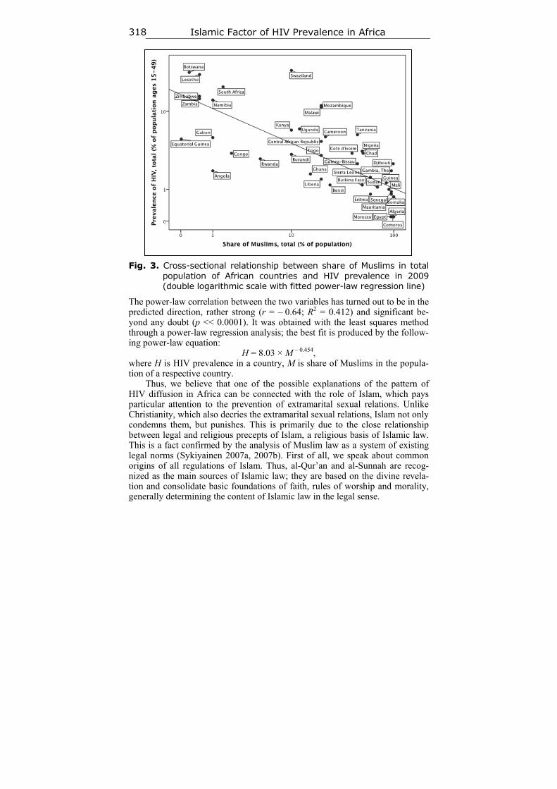
Islamic Factor of HIV Prevalence in Africa 318
Fig. 3. Cross-sectional relationship between share of Muslims in total
population of African countries and HIV prevalence in 2009 (double logarithmic scale with fitted power-law regression line)
The power-law correlation between the two variables has turned out to be in the predicted direction, rather strong (r = – 0.64; R2 = 0.412) and significant be-yond any doubt (p << 0.0001). It was obtained with the least squares method through a power-law regression analysis; the best fit is produced by the follow-ing power-law equation:
H = 8.03 × M – 0.454, where H is HIV prevalence in a country, M is share of Muslims in the popula-tion of a respective country.
Thus, we believe that one of the possible explanations of the pattern of HIV diffusion in Africa can be connected with the role of Islam, which pays particular attention to the prevention of extramarital sexual relations. Unlike Christianity, which also decries the extramarital sexual relations, Islam not only condemns them, but punishes. This is primarily due to the close relationship between legal and religious precepts of Islam, a religious basis of Islamic law. This is a fact confirmed by the analysis of Muslim law as a system of existing legal norms (Sykiyainen 2007a, 2007b). First of all, we speak about common origins of all regulations of Islam. Thus, al-Qur’an and al-Sunnah are recog-nized as the main sources of Islamic law; they are based on the divine revela-tion and consolidate basic foundations of faith, rules of worship and morality, generally determining the content of Islamic law in the legal sense.
Alisa R. Shishkina et al. 319
Its focus on the realization of the ideals of Islam as a religious system, the inclusion of a number of religious cult rules explain why Islamic law is often rightly called the quintessence, the main part of Islam, the most clear expres-sion of Muslim ideology (David 1967). In particular, the ‘concept of interest’ coming out of focus of law to defend the five core values, among which the first is given to religion, is important to understand not only the general ideo-logical framework, but also a number of legal features of Islamic law (Zayyed 1966–1967). Students of Islamic Law generally point its two characteristic and interdependent features: the religious origin (‘the divine nature’), and the close relationship of legal orders with Muslim dogma, morals and religious law of Islam in general. Famous modern specialists in the Islamic Law, such as Mu-hammad Moussa Youssuf and Subhi Mahmasani note that Islamic law is reli-gious in origin and faithful people consider it as a divine revelation (Moussa 1952). On the base of universal nature of Islam and its regulatory requirements, it is concluded that Islam is both ‘faith and state’, and Islamic Law (fiqh) is not only a law itself, but a religion as well (Mahmasani 1952). A similar point of view is expressed by many famous specialists in the Islamic Law. Thus, Joseph Schacht notes that Islamic law is characterized by the dualism of religion and state (Schacht 1966). According to R. Charle, Islamic law is primarily a religion, and then – a state and culture (Charle 1959). Islam is a religion of law, and Islamic law nature is not rational, but religious (divine), – emphasizes Rene David (David 1967). This is not applicable to Christianity where the Canon law could not be-come an imperative norm and, respectively, a part of current legislation.
Thus, we can summarize that the essential feature of Islamic law is in close dependence of its norms implementation on religious consciousness. At the same time, this approach helps to identify another important feature of socio-psychological mechanism of Islamic law implementation which explains the high efficiency of its regulatory effect on the behavior of Muslims who, in practice, in many cases refer to the norms of Islamic law as religious precepts. This is not typical for Canon law. As a consequence, Christian Canon law, in contrast to the Muslim law, could not be a part of the current legislation, in-cluding that in African countries.
Islam not only condemns extramarital sexual relations (zinā), but considers it as a serious crime (hadd) like, for example, crimes against the Ummah and infringement of the Allah rights (al-Qur’ān 4: 19–22; 7: 32; 25: 68–69; 17: 32; al-Bukhārī 2475, 6878; Muslim 57/100, 1676/25; Ibn Mājah 4019; al-Manhaj 2/40). This is due to the fact that this kind of law breaking impinges on the ba-sis of the Islamic Ummah – the family, and therefore should be punished to the fullest extent of the law. It is no accident that adultery and extramarital sexual relations are governed by the criminal law, not the Muslim family law in Africa (Al-Riahi 2011; Sykiyainen 2007a, 2007b).
Obviously, we should remember regarding this point that there exist some kind of disjuncture between religious law and beliefs and practices (see, e.g., Korotayev 2000, 2004). We can suppose that the Muslims who follow the reli-
Islamic Factor of HIV Prevalence in Africa 320
gious doctrine, and also pronouncedly worship and confirm to the rules actually have lower risk of HIV infection.
In addition, one can mention that the circumcised men suffer from HIV significantly less frequently than the non-circumcised, whereas the circumci-sion is practiced very consistently by the African Muslims (but, of course, not only African). Thus, some of epidemiological studies have shown that in high-risk sub-Saharan Africa the male circumcision that is performed for different reasons including religious, ritual, cultural, and medical, is often associated with a reduced risk of HIV infection (Bloemenkamp and Farley 2002). Although in some cases there in no sufficient evidence, the proposition about protective effect of male circumcision against HIV infection becomes more and more popular day by day, and it is regarded as one of the more powerful reducers of infection risk (Harmon 2011; Short 2006; Bonner 2007).
References
Al-Riahi N. 2011. Prostitution in the Arab World: A Legal Study of Arab Legislation. Working Paper prepared for the Middle East and North Africa Regional Consultation of the Global Commission on HIV and the Law. URL: http://www.witness-pioneer.org/vil/Books/Q_LP/.
Bloemenkamp K., and Farley T. 2002. HIV and Male Circumcision. World Health Organization International Document. Geneva: World Health Organization.
Bonner K. 2007. Male Circumcision as an HIV Control Strategy: Not a ‘Natural Condom’. Reproductive Health Matters 9(18): 143–155.
Charle R. 1959. Muslim Law. Moscow: Nauka. In Russian (Шарль Р. Мусульманское право. М.: Наука).
Chitnis A., Rawls D. et al. 2000. Origin of HIV Type 1 in Colonial French Equatorial Africa? AIDS Research and Human Retroviruses 16: 5–8.
Cliff A., and Shallman-Raynor M. 1992. The AIDS Pandemic: Global Geographical Patterns and Local Spatial Processes. The Geographical Journal 158(2): 182–198.
David R. 1967. The Main Legal Systems Today (Comparative Law). Moscow: Progress. In Russian (Давид Р. Основные правовые системы современности (сравни-тельное право). М.: Прогресс).
De Sousa D., Lemey P. et al. 2010. High GUD Incidence in the Early 20th Century Created a Particularly Permissive Time Window for the Origin and Initial Spread of Epidemic HIV Strains. PLoS ONE 5(4). URL: http://www.plosone.org/article/info% 3Adoi%2F10.1371%2Fjournal.pone.0009936.
Gao F., Bailes E. et al. 1999. Origin of HIV-1 in the Chimpanzee Pan Troglodytes Troglodytes. Nature 397(6718): 436–441.
Garenne M., and Zwang J. 2008. Premarital Fertility and HIV/AIDS in Sub-Saharan Africa. African Journal of Reproductive Health 12(2): 64–74.
Harmon K. 2011. Can Male Circumcision Stem the AIDS Epidemic in Africa? Scientific American. URL: http://www.nature.com/news/can-male-circumcision-stem-the-aids-epidemic-in-africa-1.9520.
Hiza P. 1988. International Co-operation in the National AIDS Control Programme. The Global Impact of AIDS. Proceedings of the First International Conference on the
Alisa R. Shishkina et al. 321
Global Impact of AIDS / Ed. by A. F. Fleming, et al. pp. 233–239. New York: Alan R. Liss.
Iliffe J. 2006. The African AIDS Epidemic: A History. Athens, OH: Ohio University Press.
Keele B., van Heuverswyn F., et al. 2006. Chimpanzee Reservoirs of Pandemic and Nonpandemic HIV-1. Science 313(5786): 523–526.
Korotayev A. 2000. Parallel Cousin (FBD) Marriage, Islamization, and Arabization. Ethnology 39(4): 395–407.
Korotayev A. 2004. World Religions and Social Evolution of the Old World Oikumene Civilizations: A Cross-cultural Perspective. Lewiston, NY: The Edwin Mellen Press.
Mahmasani S. 1952. Falsafat al-tashri‘ fī al-Islām. Beirut: Khayats.
Mayanja V. 1999. Openness about HIV/AIDS Slows Infection Rate in Uganda. Paris: Agency France Press.
Moore J. 2004. The Puzzling Origins of AIDS: Although No One Explanation has been Universally Accepted, Four Rival Theories Provide Some Important Lesson. American Scientist 92(6): 540–547.
Moussa M. 1952. Al-Islām wa-ḥājat al-insān ilay-hi. Falsafat al-tashrī‘ fī al-Islām / Ed. by Al-Qāhirah, Dār al-Ahrām, Maḥmāṣānī, Ṣ. Bayrūt: Khayat.
New Scientist (Ed.) 1987. Evidence for Origin is Weak. New Scientist 118(57): 27.
Piot P. et al. 1987. Retrospective Seroepidemiology of AIDS Virus Infection in Nairobi Populations. Journal of Infectious Diseases 155: 1108–1112.
Preston A., and Alcabes P. 2001. Serial Human Passage of Simian Immune Deficiency Virus by Unsterile Injections and the Emergence of Epidemic Human Immune Deficiency Virus in Africa. Philosophical Transactions of the Royal Society of London, Series B: Biological Sciences 356(1410): 911–920.
Reeves J., and Doms R. 2002. Human Immunodeficiency Virus Type 2. Journal of General Virology 83(6): 1253–1265.
Schacht J. 1966. An Introduction to Islamic Law. Oxford: Oxford University Press.
Sharp P., Bailes E, et al. 2001. The Origins of Acquired Immune Deficiency Syndrome Viruses: Where and When? Philosophical Transactions of the Royal Society of London, Series B: Biological Sciences 356(1410): 867–876.
Short R. 2006. New Ways of Preventing HIV Infection: Thinking Simply, Simply Thinking. Philosophical Transactions: Biological Sciences 361(1469): 811–820.
Sykiyainen L. 2007a. Islamic Criminal Law: From Traditional to Modern. Yearbook of Criminal Law 2: 571–596. In Russian (Сюкияйнен Л. Исламское уголовное право: От традиционного к современному. Российский ежегодник уголовного права 2: 571–596).
Sykiyainen L. 2007b. Muslim Сriminal Law: Theoretical Framework and Current Practice. Modern Criminal Law and Criminology. Moscow: INION RAN. In Russian (Сюкияйнен Л. Мусульманское уголовное право: теоретические основы и современная практика. Современное уголовное право и криминология. М.: ИНИОН РАН).
United Nations 2001. HIV/AIDS: Population Impact and Policies 2001. New York: United Nations.
Zayyed M. 1966–1967. Al-Maṣlaḥah fī al-tashrī‘ al-Islāmiyy. Al-Qāhirah, Dār al-Ahrām.
History & Mathematics: Trends and Cycles 2014 322–327
322
Contributors David G. Anderson is an archaeologist in the department of anthropology at the Uni-
versity of Tennessee, Knoxville, who specializes in Southeastern archaeology. His professional interests include exploring the development of cultural complexity in Eastern North America, maintaining and improving the nation's CRM program, teach-ing and writing about archaeology, and developing technical and popular syntheses of archaeological research. He is the project director of the on-line Paleoindian Database of the Americas. Anderson has conducted field work and led field projects in many locations in the Eastern United States, as well as projects in the Southwest and the Caribbean. His work is documented in over 200 publications, some 30 technical mon-ographs, and 7 books. Anderson has received a number of professional awards from his colleagues, including the Excellence in Cultural Resource Management Research Award from the Society for American Archaeology (1999), the Dissertation Prize from the Society for American Archaeology (1991), and the first C. B. Moore Award for Excellence in Southeastern Archaeological Studies by the Lower Mississippi Val-ley Survey / Southeastern Archaeological Conference (1990). In 2006 he was elected President-elect of the Southeastern Archaeological Conference and served as Presi-dent of that organization from 2008 to 2010. He has served as President of the South Carolina Council of Professional Archaeologists (1992–1993), The Tennessee Coun-cil for Professional Archaeology (2006–2007), and the Archaeological Society of South Carolina (1998–1999), and as an officer or board member in a number of state, regional, and national professional organizations.
David C. Baker is an Assistant Professor in Big History at the University of Amsterdam and an editor for the Paris Basin in the cliodynamics SESHAT project. He did his PhD under David Christian in Sydney, and works frequently on projects in population dynamics, cultural evolution, and the wider application of Universal Darwinism to complexity studies. He is currently script-writing for a Big History Youtube series that is funded by the Gates Big History Project and is going to be released on the channel Crashcourse later in 2014. E-mail: [email protected].
Kent Rand Crawford, Master in History, Doctor of Science, Professor of Natural His-tory. He educated in the United States, he spent much of the past ten years traveling and visiting colleagues in the United Kingdom, Spain and Russia. Now retired, he lives and works in Costa Rica, where he continues his forty plus years study of Naval Ordnance. He is the author about 50 scholarly publications, including such mono-graphs as Identification of the Parameters of Naval Artillery (in co-authorship with N. W. Mitiukov, Prague, 2013).
Sergey Gavrilets is a Distinguished Professor at the Department of Ecology and Evolu-tionary Biology and the Department of Mathematics at the University of Tennessee, Knoxville, as well as an Associate Director for Scientific Activities at the National In-stitute for Mathematical and Biological Synthesis (NIMBioS) in Knoxville. He ob-tained his PhD in Physics and Mathematics from the Moscow State University in the USSR in 1987. He subsequently worked at the Vavilov Institute of General Genet-
Contributors 323
ics in Moscow, the Institute National de la Recherche Agronomique in Toulouse, France, and the University of California at Davis, USA, before moving to Knoxville in 1995. He has received the President's Award from the American Society of Natu-ralists (1999) and the Guggenheim Fellowship (2008). He has published a monograph on the mathematical theory of speciation (in 2004) and over 100 papers. His current research interests are in speciation, human origins, and human social and societal evo-lution. E-mail: [email protected].
Leonid E. Grinin is Research Professor and the Director of the Volgograd Center for Social Research, as well as the Deputy Director of the Eurasian Center for Big History & System Forecasting, Senior Research Professor at the Institute for Oriental Studies of the Russian Academy of Sciences in Moscow and Leading Research Fellow of the Laboratory for Destabilization Risk Monitoring of the National Research University Higher School of Economics. He is the Editor-in-Chief of the journal Age of Global-ization (in Russian), as well as a co-editor of the international journals Social Evolu-tion & History and the Journal of Globalization Studies. Dr. Grinin is the author of more than 400 scholarly publications in Russian and English, including twenty six monographs. These monographs include Philosophy, Sociology, and the Theory of History (2007, in Russian); Productive Forces and Historical Process (2006, in Rus-sian); State and Historical Process (3 vols, 2009–2010, in Russian); Social Macroevo-lution: World System Transformations (2009, in Russian; with A. Korotayev); Macro-evolution in Biological and Social Systems (2008, in Russian; with A. Markov and A. Korotayev); Global Crisis in Retrospective: A Brief History of Upswings and Cri-ses (2010, in Russian; with A. Korotayev); The Evolution of Statehood: From Early State to Global Society (2011); The Cycles of Development of Modern World System (2011, in Russian; with A. Korotayev and S. Tsirel); From Confucius to Comte: The Formation of the Theory, Methodology and Philosophy of History (2012, in Rus-sian); Macrohistory and Globalization (2012); Cycles, Crises, and Traps of the Mod-ern World-System (2012, in Russian; with A. Korotayev).
Tony Harper is an independent researcher with interests in the pattern of urbanization over time and the implications of that pattern. He was a teacher at the faculty of New Trier High School for thirty-three years, during the last eleven of which he developed a strong interest in the application of math models to the study of human history. To-ny Harper was twice invited by Andrey Korotayev to take part in the conference ‘Hi-erarchy and Power in the History of Civilizations’, has recently presented at the Big History conference at Dominican University in San Rafael, California, and is continu-ing to do research in the relationship between urbanization and deurbanization. E-mail: [email protected].
Almas Heshmati is currently Professor of Economics at Jönköping University, Sweden, and Sogang University, South Korea. He held similar positions at the Korea Univer-sity, Seoul National University, and University of Kurdistan Hawler. His research in-terests include applied microeconomics, globalization, development strategy, effi-ciency, productivity and growth with application to manufacturing and services. In addition to more than 120 scientific journal articles he has published books on the EU Lisbon Process, global inequality, East Asian manufacturing, Chinese economy, tech-nology transfer, information technology, water resources, landmines, power genera-tion, development economics and economic growth. He is also Kurdish Board mem-
Contributors 324
ber of the World Kurdish Congress (South Korea). E-mail: almas.heshmati@ gmail.com.
Anthony Howell is currently a Doctoral Candidate at the Geography Department at UCLA and holds advanced degrees in both Statistics (UCLA – 2012) and Geography (Michigan State University – 2009). Trained as a statistician, urban-economic geogra-pher and China specialist, Anthony's research combines applied statistical approaches with the aid of GIS techniques and mapping of spatial relationships to develop new empirically-driven theoretical frameworks that are capable of informing social and economic policy. His dissertation research, supported by a 2012–2013 Fulbright scholarship, is a microeconomic analysis that presents new, critical information high-lighting the short- and long-run impacts of Chinese industrial policy on innovation, knowledge spillovers and firm performance. Prior to enrolling at UCLA, Anthony Howell attended Michigan State University for both undergraduate and graduate stud-ies. At MSU, he participated in 9 study/research abroad programs that provided di-verse opportunities to study Spanish and Chinese languages, volunteer with orphans and the disabled, intern, and carry out research projects in countries ranging from Mexico to Ireland, Czech Republic, United Arab Emirates and China. In summer 2006, Anthony Howell participated in an undergraduate research opportunity that took him for the first time to China, where he examined rural-urban migration patterns at the Chinese Academy of Sciences in Beijing. The culmination of his experiences in China were life-changing, both personally and professionally. Since 2006, Anthony has accumulated two-years of experience living in China, dedicating much of his time to language acquisition, and researching issues related to migration, inequality and re-gional growth.
Leonid M. Issaev is a Senior Lecturer of the General Politics Department at the Na-tional Research University Higher School of Economics, Researcher at the Laboratory for Sociopolitical Destabilization Risks Monitoring (National Research University Higher School of Economics), and Member of Scientific Council of the Russian As-sociation of Political Science. He graduated from the Faculty of Applied Political Sci-ence, the National Research University ‘Higher School of Economics’ and the Uni-versity of Cairo. He had internship at the headquarters of the League of Arab States in Cairo. He is an author of more than 60 scientific publications, including the mono-graph Egyptian Turmoil of the 21st Century (Moscow: Librokom, 2012, co-authored with A. R. Shishkina), Syria and Yemen: Unfinished Revolutions (Moscow: Libro-kom, 2012, in collaboration with A. R. Shishkina), System Monitoring of Global and Regional Risks: The Arab World After the Arab Spring (Moscow: Librokom/URSS, 2013; ed., together with A. V. Korotayev and A. R. Shishkina), and System Monitoring of Global and Regional Risks. Central Asia: New Challenges (Moscow: Librokom/ URSS, 2013, ed., together with B. A. Akayeva, A. V. Korotayev and A. R. Shishkina).
Andrey V. Korotayev is Head of the Laboratory for Destabilization Risk Monitoring of the National Research University Higher School of Economics, Senior Research Pro-fessor of the International Laboratory for Political Demography of the Russian Presi-dential Academy of National Economy and Public Administration, Senior Research Professor of the Oriental Institute and Institute for African Studies, Russian Academy of Sciences, as well as a Professor at the Faculty of Global Studies of the Moscow State University. He is the author of over 300 scholarly publications, including such
Contributors 325
monographs as Ancient Yemen (1995), World Religions and Social Evolution of the Old World Oikumene Civilizations: A Cross-Cultural Perspective (2004), Intro-duction to Social Macrodynamics: Compact Macromodels of the World System Growth (2006), and Introduction to Social Macrodynamics: Secular Cycles and Mil-lennial Trends (2006). At present, together with Askar Akaev and Sergey Malkov, he coordinates the Russian Academy of Sciences Presidium Project ‘Complex System Analysis and Mathematical Modeling of Global Dynamics’. He is a laureate of the Russian Science Support Foundation in ‘The Best Economists of the Russian Acad-emy of Sciences’ Nomination (2006).
Sergey Yu. Malkov is a Senior Research Fellow of the Institute of Economics of the Russian Academy of Sciences and a Professor of the Department of Applied Mathe-matics of the Russian State Social University. He is an author of more than 200 scien-tific publications, including such monographs as, for example, Modeling of Socio-Political and Economic Dynamics (Moscow: Russian State Social University, 2004) and Social Self-Organization and Historical Process. Possibilities of Mathematical Modeling (Moscow: Librokom/URSS, 2009). E-mail: [email protected].
Alexander V. Markov is Acting Head of the Department of Biological Evolution at Moscow State University and Senior Research Fellow of the Institute for Paleontol-ogy of the Russian Academy of Sciences. He is the author of more than 140 scientific publications in zoology, paleontology, evolution theory, historical dynamics of biodi-versity, and in other fields of evolutionary biology, including monographs: Morphol-ogy, Systematics and Phylogeny of Sea Urchins of the Schizasteridae Family (1994); Quantitative Laws of Macroevolution: Experience of Systematic Approach Use for the Analysis of Supraspecific Taxons (1998; with E. B. Neymark); Macroevolution in Bio-logical and Social Systems (2008; with Leonid Grinin, Andrey Korotayev), Hyper-bolic Growth in Biological and Social Systems (2009; with Andrey Korotayev). Dr. Markov is a member of the Editorial Board of Journal of General Biology, an au-thor of numerous popular science publications, the founder and author of the research and education portal ‘Problems of Evolution’. E-mail: http://www.evolbiol.ru.
Nicholas W. Mitiukov is Professor in Engineering, Docent, Corresponding Member of Real Academia de la Mar (Spain), Corresponding Member of the Academy of Mili-tary Science (Russia), Professor of Izhevsk State Technical University, Professor of Kama Institute of Humanitarian and Engineering Technologies. He is the author of over 500 academic publications, including such monographs as The Spanish-American War in the Pacific Ocean (in 3 volumes, St. Petersburg, 2005–2007), Simu-lation Modeling in Military History (Moscow, 2007, 2nd ed., Moscow, 2010), Ballis-tics of Arrows according to the Archeological Data (in co-authorship with A. V. Korobeinikov, Izhevsk, 2007, 2nd ed., Moscow, 2014), Identification of the Pa-rameters of Naval Artillery (in co-authorship with K. R. Crawford, Prague, 2013).
Sergey A. Nefedov is Senior Fellow at the Institute of History and Archaeology, Ural Branch of the Russian Academy of Sciences, Professor of Ural Federal University. He is the author of over 200 scholarly publications, including such monographs as De-mographic and Structural Analysis of the Socio-Economic History of Russia (2005), Factor Analysis of the Historical Process. History of the Orient (2008), Secular Cy-cles (2009, with P. Turchin), History of Russia. Factor Analysis (in 2 vols, 2010–2011). Sergey Nefedov is the winner of the ‘Social Thought’ (2008, 2011), besides he
Contributors 326
received the award named after the academician Rychkova (2011). In 2009–2011, he gave an interdisciplinary research program ‘Russian Historical Dynamics: Factors, Models, Predictions’. Е-mail: [email protected].
Arno Tausch is an Austrian citizen and in his academic functions he is Adjunct Profes-sor (Universitätsdozent) of Political Science at Innsbruck University, Department of Political Science. Currently, he is also Associate Professor of Economics, Corvinus University, Budapest, and Lecturer of International Development, Vienna University. He authored or co-authored 82 articles in peer-reviewed journals and 16 books in English, 2 in French, and 8 books in German. His publications include a number of essays for leading economic and foreign policy think tanks in nine countries, and for the Jean Monnet Institutes of the European Union in three European Union countries. E-mail: [email protected].
William R. Thompson is Distinguished Professor and Donald A. Rogers Professor of Political Science at Indiana University. His recent books include The Arc of War: Or-igins, Escalation and Transformation (2011, with Jack S. Levy), How Rivalries End (2013, with Karen Rasler and Sumit Ganguly), and Transition Scenarios: China and the United States in the Twenty-first Century (2013, with David P. Rapkin). E-mail: [email protected].
Konstantin M. Truevtsev, Associate Professor of the General Politics Department at the National Research University Higher School of Economics, Senior Fellow at the Laboratory for Sociopolitical Destabilization Risks Monitoring (National Research University Higher School of Economics). He is an author of more than 60 scientific publications, including the monographs Political System of Modern Russia (Moscow: HSE, 2004); 2011 – a New Wave of the Democratisation? (Moscow: HSE, 2011). E-mail: [email protected].
Kentaro Sakuwa is working on his PhD dissertation in the Political Science Depart-ment at Indiana University.
Alisa R. Shishkina is a Junior Research Fellow at the Laboratory for Sociopolitical Destabilization Risks Monitoring, National Research University Higher School of Economics. Alisa Shishkina is an author of more than 20 scientific works, including monographs Egyptian Turmoil of the XXI Century (Moscow: Librokom, 2012, co-authored with L. M. Issaev), Syria and Yemen: Unfinished Revolutions (Moscow: Li-brokom, 2012, in collaboration with L. M. Issaev), The Arab World in the Digital Age: Social Media as a Form of Political Activity (Moscow: Librokom/URSS, 2014, co-authored with L. M. Issaev), System Monitoring of Global and Regional Risks: The Arab World after the Arab Spring (Moscow: Librokom/URSS, 2013, ed., together with A. V. Korotayev and L. M. Issaev), and System Monitoring Global and Regional Risks. Central Asia: New Challenges (Moscow: Librokom/URSS, 2013, ed., together with B. A. Akayeva, A. V. Korotayev, and L. M. Issaev). Her sphere of scientific in-terests includes human rights, democratic transition, political processes in the modern world, sociocultural development, media studies, and the risks of social and political instability. E-mail: [email protected].
Peter Turchin was trained as a theoretical biologist, but during the last fifteen years he has been working in the field of historical social science that he and his colleagues call Cliodynamics (http://cliodynamics.info/). His research interests lie at the intersec-

Contributors 327
tion of sociocultural evolution, historical macrosociology, economic history and cli-ometrics, mathematical modeling of long-term social processes, and the construction and analysis of historical databases. More specifically, he investigates two broad and interrelated questions: What general mechanisms explain the collapse of historical empires? And how did large-scale states and empires evolve in the first place? What are the social forces that hold together huge human conglomerates, and under what conditions they fail? Turchin uses the theoretical framework of cultural multilevel se-lection to address these questions. Currently his main research effort is directed at co-ordinating SESHAT – a massive historical database of cultural evolution that will be used in empirical tests of theoretical predictions coming from various social evolution theories. Turchin has published over 100 articles in peer-reviewed journals, including over ten in Nature, Science, and PNAS. His publications are frequently cited and in 2004 he was designated as ‘Highly cited researcher’ by ISIHighlyCited.com. Turchin has authored five books. The most recent include Secular Cycles (with Sergey Nefe-dov, Princeton, 2009), War and Peace and War (Plume, 2005), and Historical Dy-namics: Why States Rise and Fall (Princeton 2003). Turchin is Editor-in-Chief of Cliodynamics: The Journal of Theoretical and Mathematical History. His blog is on the Social Evolution Forum. Web page (with a link to publications and CV): http://cliodynamics.info/Turchin.html.

History and Mathematics Guidelines for Contributors
Preparation of manuscripts. Articles should generally be no longer than 100,000 symbols. The paper's abstract should not exceed 150 words. A separate sheet should give the author's brief CV (up to 250 word). A list of keywords should be supplied. Fig-ures of good quality should be submitted as separate files.
Bibliographical references should be given in parentheses in standard author-date form in the body of the text: (Duffy, Morrison, and Macdonald 2002; Crumley 1987: 164–165; 1995: 4; 2001; Claessen 1985: 196–198, 201, 207; 2000, 2002; Chu et al. 2003: 29).
Examples of references in text: ‘In a larger population there will be proportionally more people lucky or smart
enough to come up with new ideas’ (Kremer 1993: 685); according to Rothmaler (1976: 127–129).
A complete list of references cited, arranged alphabetically by author's surname, should be typed at the end of the article along the following lines:
A) Journal articles: Schaffer W. M. 1985. Order and Chaos in Ecological Systems. Ecology 11(1): 103–109.
B) Edited volumes: Frank A. G., and Gills B. K. (Eds.) 1993. The World System: Five Hundred Years of
Five Thousand? London: Routledge.
C) Contributions to edited volumes: Humphrey N. K. 1976. The Social Function of Intellect. Growing Points in Ethology /
Ed. by P. P. G. Bateson and R. A. Hinde, pp. 303–317. Cambridge: Cambridge University Press.
D) Monographs: Berryman A. A. 1981. Population Systems: A General Introduction. New York, NY:
Plenum Press.
E) Internet resource: a) If the site does not mention the publication date:
Chase-Dunn C., and Hall T. D. 1999. The Chesapeake World-System. URL: http:// www.wsarch.ucr.edu/archive/papers/c-d&hall/asa99b/asa99b.htm. b) If possible, put the publication date:
U.S. Bureau of the Census. 2008. World Population Information. URL: http://www. census.gov/ipc/www/world.html. Date accessed: 24.02.2008.
Quotations. Single inverted commas should be used except for quotations within quotations, which should have double inverted commas. Quotations of more than 60 words should be set off from the text with an extra line of space above and below, and typed without inverted commas.
The articles are to be sent to the following email addresses: Leonid Grinin [email protected] Andrey Korotayev [email protected]
‘History and Mathematics’ homepage on our website: http://www.sociostudies. org/almanac/ham/
Related Documents