Historical (1850–2000) gridded anthropogenic and biomass ... · Received: 25 January 2010 – Published in Atmos. Chem. Phys. Discuss.: 19 February 2010 Revised: 7 July 2010 –

HAL Id: hal-00458149https://hal.archives-ouvertes.fr/hal-00458149

Submitted on 7 Jan 2016

HAL is a multi-disciplinary open accessarchive for the deposit and dissemination of sci-entific research documents, whether they are pub-lished or not. The documents may come fromteaching and research institutions in France orabroad, or from public or private research centers.

L’archive ouverte pluridisciplinaire HAL, estdestinée au dépôt et à la diffusion de documentsscientifiques de niveau recherche, publiés ou non,émanant des établissements d’enseignement et derecherche français ou étrangers, des laboratoirespublics ou privés.

Historical (1850–2000) gridded anthropogenic andbiomass burning emissions of reactive gases and

aerosols: methodology and applicationJ.-F. Lamarque, T. C. Bond, V. Eyring, Claire Granier, A. Heil, Z. Klimont,

D. Lee, C. Liousse, Aude Mieville, B. Owen, et al.

To cite this version:J.-F. Lamarque, T. C. Bond, V. Eyring, Claire Granier, A. Heil, et al.. Historical (1850–2000) griddedanthropogenic and biomass burning emissions of reactive gases and aerosols: methodology and applica-tion. Atmospheric Chemistry and Physics, European Geosciences Union, 2010, 10 (15), pp.7017-7039.�10.5194/acp-10-7017-2010�. �hal-00458149�

https://hal.archives-ouvertes.fr/hal-00458149

https://hal.archives-ouvertes.fr

Atmos. Chem. Phys., 10, 7017–7039, 2010www.atmos-chem-phys.net/10/7017/2010/doi:10.5194/acp-10-7017-2010© Author(s) 2010. CC Attribution 3.0 License.

AtmosphericChemistry

and Physics

Historical (1850–2000) gridded anthropogenic and biomass burningemissions of reactive gases and aerosols: methodology andapplication

J.-F. Lamarque1, T. C. Bond2, V. Eyring3, C. Granier4,5,6, A. Heil7, Z. Klimont 8, D. Lee9, C. Liousse10, A. Mieville6,B. Owen9, M. G. Schultz7, D. Shindell11, S. J. Smith12, E. Stehfest13, J. Van Aardenne14, O. R. Cooper4,M. Kainuma 15, N. Mahowald16, J. R. McConnell17, V. Naik18, K. Riahi8, and D. P. van Vuuren13

1National Center for Atmospheric Research, Boulder, USA2University of Illinois, Urbana-Champaign, IL, USA3Deutsches Zentrum fuer Luft- und Raumfahrt (DLR), Institut fur Physik der Atmosphare, Oberpfaffenhoffen, Germany4NOAA Earth System Research Laboratory, Chemical Sciences Division, Boulder, CO, USA5Cooperative Institute for Research in Environmental Sciences, University of Colorado, Boulder, Colorado, USA6UPMC Univ. Paris 06; CNRS/INSU, UMR 8190 LATMOS-IPSL, Paris, France, France7Forschungszentrum, Julich, Germany8International Institute for Applied Systems Analysis, Laxenburg, Austria9Manchester Metropolitan University, Manchester, UK10Laboratoire d’Aerologie, Toulouse, France11Goddard Institute for Space Studies, National Aeronautics and Space Agency, New York, NY, USA12Joint Global Change Research Institute, Pacific Northwest National Laboratory, College Park, MD, USA13Netherlands Environmental Assessment Agency, Bilthoven, The Netherlands14European Commission, DG, Joint Research Center, Ispra, Italy15National Institute of Environmental Studies, Tsukuba, Japan16Cornell University, Ithaca, New York, USA17Desert Research Institute, Reno, Nevada, USA18High Performance Technologies Inc./NOAA Geophysical Fluid Dynamics Laboratory, Princeton, NJ, USA

Received: 25 January 2010 – Published in Atmos. Chem. Phys. Discuss.: 19 February 2010Revised: 7 July 2010 – Accepted: 9 July 2010 – Published: 3 August 2010

Abstract. We present and discuss a new dataset of grid-ded emissions covering the historical period (1850–2000) indecadal increments at a horizontal resolution of 0.5◦ in lati-tude and longitude. The primary purpose of this inventory isto provide consistent gridded emissions of reactive gases andaerosols for use in chemistry model simulations needed byclimate models for the Climate Model Intercomparison Pro-gram #5 (CMIP5) in support of the Intergovernmental Panel

Correspondence to:J.-F. Lamarque([email protected])

on Climate Change (IPCC) Fifth Assessment report (AR5).Our best estimate for the year 2000 inventory represents acombination of existing regional and global inventories tocapture the best information available at this point; 40 re-gions and 12 sectors are used to combine the various sources.The historical reconstruction of each emitted compound, foreach region and sector, is then forced to agree with our 2000estimate, ensuring continuity between past and 2000 emis-sions. Simulations from two chemistry-climate models areused to test the ability of the emission dataset describedhere to capture long-term changes in atmospheric ozone,carbon monoxide and aerosol distributions. The simulated

Published by Copernicus Publications on behalf of the European Geosciences Union.

http://creativecommons.org/licenses/by/3.0/

7018 J.-F. Lamarque et al.: 1850–2000 gridded anthropogenic and biomass burning emissions

long-term change in the Northern mid-latitudes surface andmid-troposphere ozone is not quite as rapid as observed.However, stations outside this latitude band show much bet-ter agreement in both present-day and long-term trend. Themodel simulations indicate that the concentration of carbonmonoxide is underestimated at the Mace Head station; how-ever, the long-term trend over the limited observational pe-riod seems to be reasonably well captured. The simulatedsulfate and black carbon deposition over Greenland is in verygood agreement with the ice-core observations spanning thesimulation period. Finally, aerosol optical depth and addi-tional aerosol diagnostics are shown to be in good agreementwith previously published estimates and observations.

1 Introduction

In order to perform climate simulations over the historicalrecord, it is necessary to provide climate models with in-formation on the evolution of radiatively active gases andaerosols. In particular, tropospheric ozone and aerosols ofanthropogenic and biomass burning origins (sulfate, nitrate,black carbon and organic carbon) constitute the species of in-terest in our study. Climate models that will contribute to sce-nario analysis for IPCC AR5 report (Intergovernmental Panelon Climate Change; Fifth Assessment Report) usually starttheir model calculations in pre-industrial times, specified inthis case as being 1850 (Taylor et al., 2009). As will be iden-tified later in our study, it is however clear that anthropogenicemissions were already significantly present in 1850. In or-der to enable climate model simulations, knowledge of theevolution of the necessary emissions between 1850 and 2000is required. And it is the purpose of this study to discuss thedefinition of such an emission data set, based on the combi-nation of new and existing efforts. It is important to note thatthe data set discussed in this study is primarily developed fordefining the distribution and time evolution of short-lived cli-mate forcing agents and not for regional air quality models.

Examples of gridded emissions can be found at theGEIA/ACCENT emissions portal (available at:http://geiacenter.org). The determination of these emissions re-quire a variety of steps involving the knowledge of the sourceof emission (e.g. amount of fossil fuel combusted by powerplants), an emission factor (e.g. how much of a given chem-ical species is emitted for a specific mass of a given fuelburned in a specific technological process accounting forthe operation of abatement measures) and a procedure formapping onto a geographical grid (e.g. the location pointsources such as power plants). As discussed in Klimont andStreets (2007) the quality of available emission inventoriesvaries, between high quality inventories for point sources inEurope or North America (e.g. SO2 from power plants whichis based on emission monitoring) and inventories that areless reliable, especially in developing or industrializing coun-

tries due to incompleteness of activity data or lack of test-based emission factors. The resulting uncertainty leads to arange of possible emissions for a given process and base yearthat varies strongly between regions, sectors, and pollutants(e.g. Streets et al., 2006; Klimont and Streets, 2007; Bondet al., 2007). These uncertainties lead to a range of possibleemission outcomes for a given source. While this issue ap-plies to all types of emissions, we will focus in this paper onanthropogenic (defined here as originating from energy usein stationary and mobile sources, industrial processes, do-mestic and agricultural activities) and open biomass burningemissions. Our overall approach to building this new emis-sion dataset is to combine a variety of data sources to maxi-mize the information content; this is done through a combi-nation of (1) regional and global inventories in order to de-fine year 2000 emissions and (2) long-term global emissiondatasets to define historical changes in emissions.

In order to perform chemistry simulations with enoughresolution to resolve regional structures and their changes,our target is to provide monthly emissions at a horizontalresolution of 0.5◦ in latitude and longitude every 10 years.All anthropogenic and biomass burning emissions necessaryfor the simulation of tropospheric ozone and aerosols areprovided, including methane (CH4), carbon monoxide (CO),nitrogen oxides (NOx), total and speciated non-methanevolatile organic compounds (NMVOCs), ammonia (NH3),organic carbon (OC), black carbon (BC) and sulfur diox-ide (SO2). Compounds relevant for other issues (e.g. CFCs,HCFCs and HFCs, mercury, persistent organic pollutants)have not been included in this inventory as they were notnecessary for the stated goal of providing climate modelsdistributions of tropospheric ozone and aerosols for radia-tive forcing. While interannual changes may be importantfor the detailed analysis of past “rapid” (i.e. less than a fewyears) pollution changes, we decided that decadal data areoverall better suited to fulfill the needs of AR5 for the fol-lowing reasons: (1) annual data sets exist only for a limitedset of species (Smith et al., 2004) or only for the recent past– for example RETRO, available for the 1960–2000 period(Schultz et al., 2007, 2008) and REAS, which covers the1980–2003 (Ohara et al., 2007; Smith et al., 2004) and (2) fu-ture emissions generated by Integrated Assessment Models(IAMs) are usually available with time steps on the order of10 years.

Gridding follows the sectoral grids generated for EDGAR-v4 (EC-JRC/PBL, 2009), averaged from its original 0.1◦

resolution to our nominal 0.5◦ grid. While this is clearlyadequate for present-day, such gridding will not be rep-resentative of older emission distributions. We are there-fore performing two separate griddings: one from EDGAR-v4, the other based solely on population (Goldewijk, 2005).The final gridding is a linear combination of both, with theEDGAR-v4 component linearly increasing in time after 1900to 1980, after which the EDGAR-v4 grids are used.

Atmos. Chem. Phys., 10, 7017–7039, 2010 www.atmos-chem-phys.net/10/7017/2010/

http://geiacenter.org

http://geiacenter.org

J.-F. Lamarque et al.: 1850–2000 gridded anthropogenic and biomass burning emissions 7019

Table 1. List of multi-decadal inventories used in this study.

EDGAR-HYDE RETRO Smith et al. Bond et al. Junker andEDGAR Liousse

Species 1890–2000 1960–2000 1850–2000 1850–2000 1860–1997

CH4 XCO X XNOx X XNMVOC X XNH3 XSO2 XOC X XBC X X

Finally, we have decided to include seasonal variations (atthe monthly scale) for biomass burning, soil NOx, ship andaircraft emissions only. Other emissions, while gridded ona monthly basis, have constant values for each month. Wehave indeed considered that there as insufficient informationavailable (especially for past emissions) on the seasonality toimpose a temporal profile; we therefore prefer the end-userto assign such a seasonal variation if preferred.

The paper is organized as follows: in Sect. 2, we dis-cuss the land-based anthropogenic emissions, defined here asoriginating from industrial, domestic and agriculture activitysectors. Section 3 described the biomass burning emissions.In Sect. 4, we present our reconstruction of ship and air-craft emissions. Application of these emissions in chemistry-climate models and the analysis of the modeled concentra-tions of ozone carbon monoxide and aerosols are discussedin Sect. 5. Finally, discussion and conclusions are in Sect. 6.

2 Land-based anthropogenic emissions

In the case of land-based anthropogenic emissions (i.e., ex-cluding aircraft and ship emissions), two available datasetson historical emissions, RETRO (1960–2000; Schultz et al.,2007) and EDGAR-HYDE (1890–1990; van Aardenne et al.,2001), provide information on emission changes over thesecond half of the 20th century for a limited set of com-pounds (Table 1). As mentioned in the Introduction, our ap-proach consists of generating first our best estimate for 2000,based on the combination of global and regional datasets.This aggregation is performed using a set of 40 regions (Ta-ble 2) and 12 sectors (Table 3). Then, using a combination ofRETRO and EDGAR-HYDE, historical trends for each sec-tor in each region are generated. Finally, the historical emis-sions of reactive gases (ozone precursors only) are computedusing the historical trends applied to our 2000 emissions. Wediscuss those three steps in this section.

Table 2. List of regions.

Region number Name of Region

1 Canada2 USA3 Mexico4 Rest of Central America5 Brazil6 Venezuela7 Argentina8 Rest of South America9 Northern Africa10 Western Africa11 Eastern Africa12 Rest of Southern Africa13 South Africa14 France15 Germany16 Italy17 UK18 Rest of Western Europe19 Rest of Central Europe20 Baltic States (Estonia, Latvia, Lithuania)21 Turkey22 Ukraine23 Kazachstan region24 Russia25 Middle East26 India27 Rest of South Asia28 South Korea (Republic of Korea)29 North Korea (Democratic People’s Republic of Korea)30 China31 Taiwan32 Thailand33 Rest of Southeastern Asia34 Indonesia35 Japan36 Australia37 New Zealand38 Rest of Oceania39 Greenland40 Antarctica

www.atmos-chem-phys.net/10/7017/2010/ Atmos. Chem. Phys., 10, 7017–7039, 2010


Table 3. List of sectors.

Sector number Sector name

1 Energy production and distribution2 Industry (combustion and non-combustion)3 Land transport4 Maritime transport5 Aviation6 Residential and commercial7 Solvents8 Agriculture9 Agricultural waste burning on fields10 Waste11 Open vegetation fires in forests12 Open vegetation fires in savanna and grasslands

While several recent assessments have shown that re-gional emissions have experienced significant changes be-tween 2000 and present, especially in South Asia (e.g.,Richter et al., 2005; Zhang et al., 2009; Klimont et al., 2009),the necessity to rapidly generate an inventory that could beused as a basis for the future projections using Integrated As-sessment Models for the upcoming IPCC AR5 required thatthe latest year we felt we could confidently use (as of late2008) was the year 2000. The additional information fromthe references cited above are taken into account in the pro-jections for 2005 which will be discussed elsewhere.

2.1 Definition of year 2000 emission

Anthropogenic emissions of reactive gases in 2000 are de-fined in terms of a variety of global and regional inven-tories (Table 4). In generating our emission dataset, pub-lished or reviewed regional inventories have been given pref-erence over global inventories where these were available.This was the case for the EMEP (2006) inventory for Eu-rope, the REAS inventory for Asia and the EPA inventoryfor North America. In those regions we assume that these in-ventories more appropriately reflect regional circumstancesthan the global inventories. Furthermore, the inventories forNorth America and European countries within the EMEP do-main have been extensively evaluated through model and ob-servation studies. In addition, inventories reported as An-nex I inventories to the United Nations Framework Conven-tion on Climate Change (UNFCCC) are subject to expert re-view. The EDGARv32 FT2000 dataset (Van Aardenne et al.,2005; Olivier et al., 2005) and preliminary emissions fromEDGAR v4.0 for agriculture (EC-JRC/PBL, 2009) are usedwhere regional information is not available. A summary isgiven in Table 4. As the various inventories are combined atthe level of regional averages, no attempt is made at smooth-ing potential discontinuities across regional boundaries.

Following the new sectoral definition in EDGAR-v4, wehave included the contribution from biofuel combustion (forcooking and heating) in the residential sector (Table 3). Agri-cultural waste burning is therefore restricted to the burningof biomass left on the fields. Our global estimate for 2000of those latter emissions are in good agreement with the pub-lished estimate of Yevich and Logan (2002).

Although additional information is available in the litera-ture for several regions (e.g., Zhang et al., 2009; Streets etal., 2003, 2006; Klimont et al., 2009; Cofala et al., 2007;NARSTO, 2006; Garg et al., 2006), we did not attempt to in-clude those as they were already integrated into the datasetswe have used (e.g., for East Asia REAS includes resultsof several specific inventories) or, less frequently, were lesscomplete than the inventories applied in this study (e.g. onlycovering 1 country or did not extend to the year 2000).

The specific case of regional carbon monoxide emissionsis highlighted in Table 5. In this case, we see that the ouremission inventory is well within the range of published esti-mates at the regional and global scales. Agreement for otherspecies is found to be similar or better (not shown). Emis-sions of black carbon (BC) and organic carbon (OC) includedin the dataset presented here (Table 4) represent an update ofBond et al. (2007) and Junker and Liousse (2008) as harmo-nization of emission factors was performed for the year 2000from these papers and the studies they reference; more de-tails are presented in the next section.

Emissions from the UNFCCC Emissions of sulfur dioxidesubmissions and other regional inventories were used whereavailable (Table 4). Bottom-up estimates of emissions areused where inventory data were either unavailable or incon-sistent. Details are given in Smith et al. (2010).

For all species, gridding is performed using theEDGAR v4.0 spatial distribution maps specific for each sec-tor at a 0.1◦ resolution, and aggregated to a 0.5◦ grid (EC-JRC/PBL, 2009). The 2000 SO2 map used additional datafrom EDGARv32 FT2000 for smelting and fuel processingemissions.

2.2 Historical reconstruction

As we have two distinct long-term emission datasets forozone precursors (RETRO and EDGAR-HYDE) with dif-fering trends and there is no a priori reason to choose oneinventory over the other, we have devised an approach thatmaximizes the information from both datasets where applica-ble. Using the RETRO and EDGAR-HYDE historical trendsper region and per sector, we generate historical trends foreach sector in each region by defining the ratio of the emis-sions at a specific decade to its value in 2000 (our refer-ence data set). This ratio is a concise representation of thecombined changes in fuel use and emission factor over timeand its full history (1850–2000) that can be used to scaleour 2000 inventory to define emissions in previous decades.The scaling of the anthropogenic emissions for reactive gases



Table 4. Primary source of information for the various regional inventories used in the definition of the 2000 dataset.

Region Ozone prec. SO2 OC/BC NH3

Asia Cofala et al., 2007 Smith et al., 2010 Bond et al., 2007 EDGAR-v4Europe EMEP UNFCCC Bond et al., 2007 EDGAR-v4United States EPA EPA Bond et al., 2007 EDGAR-v4Japan, Australia, NZ UNFCCC UNFCCC Bond et al., 2007 EDGAR-v4Canada Env. Canada Env. Canada Bond et al., 2007 EDGAR-v4Latin America EDGAR-v4 Smith et al., 2010 Bond et al., 2007 EDGAR-v4South America EDGAR-v4 Smith et al., 2010 Bond et al., 2007 EDGAR-v4Other regions EDGAR-v4 Smith et al., 2010 Bond et al., 2007 EDGAR-v4

Table 5. Regional and global estimate of year 2000 CO anthropogenic and biomass burn-ing emissions (Tg(CO)/year). This table uses data from the following: EDGAR–FT2000:http://www.mnp.nl/edgar/model/v32ft2000edgar/docv32ft2000/;RETRO: http://retro.enes.org/pubreports.shtml; GAINS: Cofala etal., 2007; EPA–2006: http://www.epa.gov/airtrends/2006/emissionssummary2005.html; EMEP–2004: Vestreng et al., Technical ReportNSC–W 1/2004; TRACE–P: Streets et al., 2003; GFED–v2: Randerson et al., 2005; GICC: Mieville et al., 2010.

Anthro. EDGAR-FT2000 RETRO GAINS EPA-2006 EMEP-2004 TRACE-P This work

Global 548 476 542 N/A N/A N/A 611US 74 56 75 102 N/A N/A 93W. Europe 30 19 38 N/A 31 N/A 31China 98 95 128 N/A N/A 100 121

Bio. burn. GFED-v2 GICC This work

Global 427 467 459

(excluding SO2) using EDGAR-HYDE and RETRO relieson the assumption that each reconstruction provides a reason-able (albeit sometimes different) representation of the timeevolution of emissions; this can clearly only be applied tospecies available in both emission datasets, i.e. CO, NOx andNMVOCs. The main differences between the RETRO andEDGAR-HYDE datasets are in the emission factors varia-tions over time (with RETRO having more technology in-formation) and, to a lesser extent, the completeness of theinventory (e.g. no industrial process emissions in RETRO).Therefore, emissions for decades prior to 2000 can be calcu-lated through a direct scaling (per sector and region) of our2000 emissions, with a weighting factor defined as a linearcombination of the RETRO and EDGAR-HYDE scaling fac-tors, increasingly favoring EDGAR-HYDE when going fur-ther back in time (as RETRO is only available from 1960).To provide emissions back to 1850, EDGAR-HYDE emis-sions (which cover 1890 to 1990) are extrapolated to 1850using global fossil fuel consumption estimates from Andreset al. (1999) and regional scale data for population from theHYDE dataset (Goldewijk, 2005).

In summary, the scaling for each sector and region is com-puted using the following steps:

1. The 1990–2000 change is computed in RETRO only(since the year 2000 is not included in EDGAR-HYDE).

2. The decadal changes between 1960 and 1990 are a com-bination of RETRO and EDGAR-HYDE.

3. The decadal changes between 1890 and 1960 are com-puted from EDGAR-HYDE only (no RETRO estimatesprior to 1960).

4. The emissions between 1850 and 1890 are exactly ascomputed from EDGAR-HYDE and its extrapolation.

5. Smoothing is applied to scaling factors across 1960 and1990 to limit jumps in the scaling factor.

The advantage of using a scaling approach is that it only re-quires that the existing emission inventories provide a timehistory of the specific emission, without having to deal withemission biases between inventories. Clearly, such historyis meaningful only within a particular sector and for a spe-cific region as pollution controls vary; the scaling therefore



Table 6. Recent trend in US emissions (Tg(species)/year;NOx expressed as NO2). Data are available from: EPA–2003:http://www.epa.gov/oar/aqtrnd03/appenda.pdf;EPA--2006:http://www.epa.gov/airtrends/2006/emissionssummary2005.html;EDGAR–HYDE: van Aardenne et al. (2001); RETRO:http://retro.enes.org/pubreports.shtml.

1970 CO NOx Total VOCs SO2

EDGAR-HYDE 84.2 16.6 19.4 N/ARETRO 115.5 19.1 * N/AEPA-2003 N/A N/A N/A N/AEPA-2006 197.3 26.9 33.7 31.2This work 79.9 16.5 25.8 27.0

1980 CO NOx Total VOCs SO2EDGAR-HYDE 90.2 19.0 22.4 N/ARETRO 109.3 20.3 * N/AEPA-2003 105.7 22.0 23.7 23.3EPA-2006 177.8 27.1 30.1 25.9This work 118.8 19.8 25.4 22.2

1990 CO NOx Total VOCs SO2EDGAR-HYDE 95.1 21.8 24.2 N/ARETRO 96.4 19.1 * N/AEPA-2003 89.2 21.8 18.9 21.3EPA-2006 143.6 25.2 23.1 23.1This work 112.1 20.6 23.8 19.0

2000 CO NOx Total VOCs SO2EDGAR-HYDE N/A N/A N/A N/ARETRO 55.7 18.5 * N/AEPA-2003 98.4 22.4 18.3 16.2EPA-2006 102.4 22.3 16.9 16.3This work 93.0 19.6 15.2 14.8

captures the change in fuel amount (usually fairly well-constrained) and change in the emission factors. It also relieson the assumption of an unbiased 2000 estimate; however, ifsuch a bias were to be present, the methodology presentedhere could be applied to an updated set of 2000 estimates.

Results from this scaling process are illustrated in Table 6where the generated time evolution is compared with pre-visouly published estimates. Because of the completenessof data available from the US EPA and the importance ofthose emissions, we focus our analysis on those emissions.We see that, as discussed earlier, our estimates for 2000 arein good agreement with the EPA data. The largest discrep-ancy occurs with the CO emissions going back to 1970. Itis however critical to note that the EPA estimates, with emis-sions largely driven by the transportation sector, are poten-tially over-estimated, based on the independent analysis ofParrish (2006). Indeed, this paper shows that the use of sur-face observations of CO strongly suggests an overestimate(by a factor of 2) in the EPA-2004 data (and 2006) as far

back as 1970. In the Parrish paper, the CO observed trendsand values seem to be in better agreement with the EPA-2003(and older) data, and therefore in quite good agreement withour estimates. Other species have a smaller spread in their es-timated emissions and our inventory is consistent with those.

While there can be wide variations for a specific sectoror region, the global total amounts of anthropogenic emis-sions for each compound are actually quite similar to eitherRETRO or EDGAR-HYDE (Fig. 1 and Table 7), except forNMVOCs. The largest difference (in absolute amounts) is anincrease in CO emissions compared to the EDGAR-HYDEestimate. Emissions of nitrogen oxides are quite similar be-tween the two original inventories; in particular, the emis-sions between 1960 and 1980 are almost identical in RETROand EDGAR-HYDE. Our combined dataset ends up slightlyhigher over that time period because our 2000 NOx emis-sion estimate is larger than in RETRO. On the other hand,our 2000 NMVOC emissions are smaller than either RETROor EDGAR-HYDE, again with a peak in 1990, similar toRETRO.

For OC and BC, the inventory structure was based largelyon the structure presented in Bond et al. (2004) and the time-varying technology divisions in Bond et al. (2007). Newinformation on emission factors has become available sincethat time and these were incorporated. Several new studieson emission factors have become available in recent years:domestic coal burning emission factors were updated basedon an extensive study in China (Chen et al., 2005, 2006;Zhi et al., 2008). Domestic biofuel now includes the lab-oratory reports of Venkataraman et al. (2005) and Parasharet al. (2005) and field data from Roden et al. (2006, 2007),Johnson et al. (2008); ship emission factors are now takenfrom Sinha et al. (2003), Lack et al. (2008) and Petzold etal. (2008). Black carbon fractions for two-stroke enginesare from Volckens et al. (2008); emission factors for cementkilns are added based on the US EPA compilation of emis-sion factors (AP-42, 1996), and black and organic carbonfractions from US EPA’s SPECIATE database (2004).

We have performed a sector-by-sector comparison toresolve differences between the inventories of Bond etal. (2007) and Junker and Liousse (2008). Because of differ-ing treatments of emission factors, black carbon emissionsfrom fossil fuels are about twice as great in the latter inven-tory. The largest sectoral difference between the inventorieswas in power generation, where emission factors were twoorders of magnitude higher in Junker and Liousse (2008).Relevant measurements were compiled and the two groupsagreed on an intermediate emission factor. With the consen-sus emission factors, power generation contributes less than1% of total black carbon emissions.

In addition, for all decades, emissions of OC and BC fromagricultural waste burning were computed from the CO es-timate of agricultural waste burning at each decade scaledusing regional emission factor (OC/CO and BC/CO) basedon our 2000 emission estimates of OC, BC and CO.


http://www.epa.gov/oar/aqtrnd03/appenda.pdf; EPA--2006: http://www.epa.gov/airtrends/2006/emissions_summary_2005.html

http://www.epa.gov/oar/aqtrnd03/appenda.pdf; EPA--2006: http://www.epa.gov/airtrends/2006/emissions_summary_2005.html

http://retro.enes.org/pub_reports.shtml


CO NOx NMVOC

EDGAR

RETRO

This work

Fig. 1. Time evolution of the total (sum of all sectors but agricultural waste burning) land anthropogenic emissions for CO (Tg(CO)/year),NOx (Tg(NO2)/year) and total NMVOC (Tg(NMVOC)/year).

Table 7. Global amounts of emission from anthropogenic sourcesfor each species considered in this study

Year CO NOx VOC BC OC NH3 SO2

1850 63.04 1.24 10.16 1.05 4.63 6.55 2.021860 67.26 1.59 10.46 1.25 5.27 7.34 2.951870 76.60 2.23 12.15 1.49 5.83 7.40 4.621880 85.99 2.88 13.85 1.71 6.20 7.47 7.671890 95.66 3.55 15.62 1.99 6.51 7.54 12.611900 111.11 4.60 18.48 2.31 6.82 8.62 19.821910 132.79 6.24 20.99 2.79 7.50 9.20 30.091920 153.03 7.42 23.46 2.98 7.76 10.85 33.181930 182.76 9.18 27.41 2.81 8.07 12.20 41.291940 206.59 10.81 31.17 2.86 8.69 12.88 49.961950 277.91 17.24 43.35 2.91 8.78 16.97 56.961960 376.54 25.40 70.36 3.22 9.78 20.82 87.311970 474.43 36.49 101.16 3.34 10.25 26.48 117.651980 583.75 51.84 126.75 4.51 10.98 35.18 120.331990 626.76 59.24 137.50 4.81 11.91 42.61 116.112000 608.28 56.77 129.53 5.02 12.56 37.46 92.71

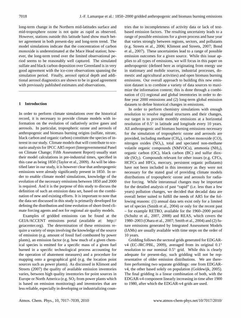
For NH3 we use the reconstruction by Beusen et al. (2008)while for CH4, since only one historical inventory (EDGAR-HYDE) exists, the only constraint to the present emissiondataset comes from our 2000 estimate.

Emissions of sulfur dioxide are an update of Smith etal. (2001, 2004), with emissions from the UNFCCC sub-missions and other regional inventories used where available.Bottom-up estimates of emissions are used where inventorydata was either unavailable or inconsistent. Details are givenin Smith et al. (2010).

Soil emissions of nitrogen oxides are clearly affected bythe use of fertilizers; it is therefore difficult to disentangle thenatural and anthropogenically-perturbed components to thisflux. In the present work, the 2000 anthropogenic portion (in-cluded in the agricultural sector) is estimated in EDGAR-v4.To extend this to prior decades, we have used the EDGAR-HYDE estimate of soil NOx emissions prior to 1950 (i.e. be-fore strong growth in man-made fertilizer use; Erisman etal., 2009) to define the natural component. The long-term

time evolution (applied to our 2000 estimate and correctedfor the natural contribution) is based on the results from Yanet al. (2005). In addition, the seasonal cycle (available ata monthly scale) is taken from the 2000 data from Yan etal. (2005) and applied to all decades.

For all ozone precursors and NH3 (OC/BC and SO2 aregridded separately based on their respective previous meth-ods), gridding of the emissions for the 1850–2000 period re-lies on a weighted mean of the distributions obtained usingeither population (from the HYDE dataset) or the year 2000gridded emissions provided by EDGAR-v4. It is applied sothat the weighting associated with the 2000 gridded distri-butions decreases when going back in time, with emissionsafter 1980 using the same grid as 2000; this is based on theassumption that, within a region, heavy infrastructure (suchas power plants) has a very long (decades) lifespan. Althoughthis approach might lead in few specific areas to shifts insource allocation (e.g., the collapse of several economies inEastern Europe in the 1990s “removed from the map” sev-eral industrial sources), we believe this has only limited im-pact on the simulations intended using these historical sets ofdata.

No vertical emission profile is provided; however, theavailability of sectoral emissions (energy, industry, domes-tic, etc.) in our emission files allows consistent assumptionsabout stack height to be applied if desired.

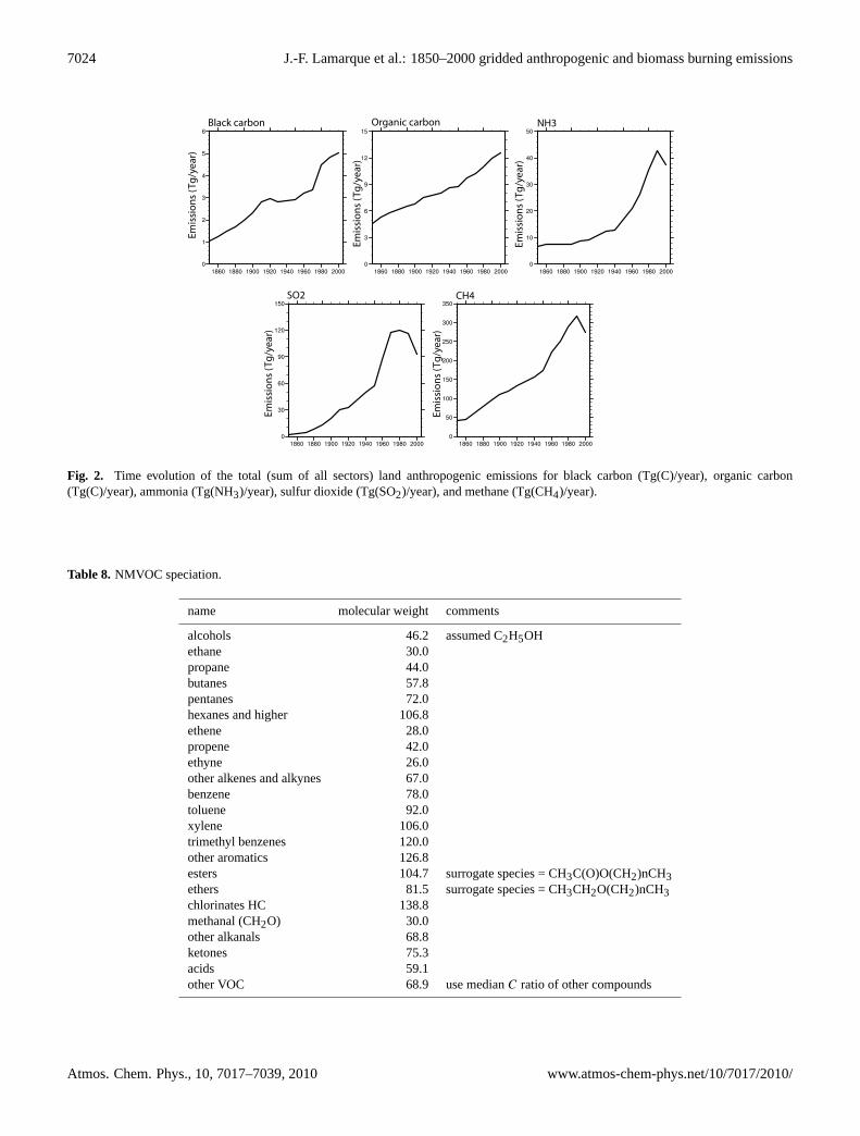
Speciation of NMVOC emissions is performed using theRETRO inventory. In this case, regional information for thesplit of the total NMVOC emitted into a set of specific hy-drocarbons (Table 8) is available for the year 2000. Becauseof the lack of additional information, the same ratio (specifichydrocarbon to total NMVOCs at each grid point) is keptconstant for the whole historical period.

3 Biomass burning emissions

Only a few inventories provide biomass burning emissionsfor the past decades (Ito and Penner, 2005; Schultz et al.,2008; Mieville et al., 2010). In this paper, we focus onthe following: (1) the RETRO inventory (Schultz et al.,



Black carbon Organic carbon NH3

SO2 CH4

Emis

sio

ns

(Tg

/yea

r)

Emis

sio

ns

(Tg

/yea

r)

Emis

sio

ns

(Tg

/yea

r)

Emis

sio

ns

(Tg

/yea

r)

Emis

sio

ns

(Tg

/yea

r)

Fig. 2. Time evolution of the total (sum of all sectors) land anthropogenic emissions for black carbon (Tg(C)/year), organic carbon(Tg(C)/year), ammonia (Tg(NH3)/year), sulfur dioxide (Tg(SO2)/year), and methane (Tg(CH4)/year).

Table 8. NMVOC speciation.

name molecular weight comments

alcohols 46.2 assumed C2H5OHethane 30.0propane 44.0butanes 57.8pentanes 72.0hexanes and higher 106.8ethene 28.0propene 42.0ethyne 26.0other alkenes and alkynes 67.0benzene 78.0toluene 92.0xylene 106.0trimethyl benzenes 120.0other aromatics 126.8esters 104.7 surrogate species = CH3C(O)O(CH2)nCH3ethers 81.5 surrogate species = CH3CH2O(CH2)nCH3chlorinates HC 138.8methanal (CH2O) 30.0other alkanals 68.8ketones 75.3acids 59.1other VOC 68.9 use medianC ratio of other compounds



2008) provides emissions from wildfires for each year dur-ing the 1960–2000 period, on a monthly basis; (2) theGICC inventory (Mieville et al., 2010) gives emissions fromopen biomass burning for the 20th century (1900–2000) ona decadal basis based on Mouillot et al. (2005); (3) theGFEDv2 inventory (van der Werf et al., 2006) covers emis-sions for the 1997–2006 period.

For our study, we have established a best estimate of his-toric biomass burning emissions from a combination of threedatasets: the GICC inventory is used as input data for theconstruction of the 1900–1950 dataset, the RETRO inven-tory for the 1960–1990 dataset and the GFEDv2 inventoryfor the 2000 estimate. The GFEDv2 inventory was favoredover the 2000 estimate from RETRO because it is one of themost state-of-the art global biomass burning dataset currentlyavailable that incorporates satellite-based burned area esti-mates and seasonality.

Given the substantial interannual variability of biomassburning on a global and regional scale (e.g., Duncan et al.,2003; Schultz et al., 2008), it is problematic to use a snap-shot dataset from an individual year for the development ofa dataset that is considered to be representative for a decade.We therefore decided to construct historic gridded biomassburning emissions from decadal means (years 0 to 9 of agiven decade), except for the 2000 estimate which is calcu-lated from the 1997–2006 average.

In order to enforce consistency of biomass burning emis-sions over the entire period, carbon emission fluxes from thethree datasets are first harmonized, taking the 2000 estimatefrom GFEDv2; emissions of trace gases and aerosols arethen re-calculated from the gridded carbon emission fluxesprovided in the three datasets by applying a single set ofvegetation-type specific emission factors. The vegetationcover map is derived from the MODIS predominant vege-tation cover map as provided with the GFEDv2 inventory(van der Werf et al., 2006). It contains a classification of theyear 2000 vegetation into the major vegetation classes sa-vanna/herbaceous vegetation, tropical forest and extratropi-cal forest. The emission factors for these classes were harmo-nized to those given by Andreae and Merlet (2001, with up-dates from M. O. Andreae, personal communication, 2008).

Emissions from burning of soil organic matter, notablypeat soil, which is ignited by fires in the overlying surfacevegetation, may strongly influence emission production insome boreal and tropical regions (Page et al., 2002; Kasis-chke et al., 2005). Therefore, peat fires are explicitly takeninto account in our inventory. We assumed that peat fires cancontribute up to 45% to the total carbon emissions releasedper grid cell if the fractional peat cover is 100%. If the frac-tional peat cover is lower, the relative contribution of carbonemissions from fires in surface vegetation increases accord-ingly. Note that this is an update from the original RETROinventory. Information on the fractional distribution of peatsoils is taken from the FAO (2003) WRB Map of World SoilResources. The assumed maximal contribution of peat fires

Table 9. Global amounts of emission from biomass burning foreach species considered in this study. Tg(species)/year except forNOx which is expressed as Tg(NO)/year.

Year CO NOx VOC BC OC NH3 SO2

1850 322.55 10.36 51.81 2.03 17.99 6.14 2.451860 322.55 10.36 51.81 2.03 17.99 6.14 2.451870 322.55 10.36 51.81 2.03 17.99 6.14 2.451880 322.55 10.36 51.81 2.03 17.99 6.14 2.451890 322.55 10.36 51.81 2.03 17.99 6.14 2.451900 322.44 10.36 51.81 2.03 17.99 5.80 2.441910 315.18 10.04 50.78 1.97 17.60 5.85 2.431920 277.97 9.05 44.52 1.78 15.14 4.84 2.061930 276.30 9.07 44.15 1.79 14.94 4.68 2.011940 267.19 8.86 42.57 1.75 14.25 4.37 1.901950 260.79 8.74 41.43 1.74 13.70 4.12 1.821960 286.46 8.12 47.54 1.81 14.57 4.81 2.031970 333.81 9.40 55.51 2.10 16.86 5.68 2.371980 383.22 10.28 64.54 2.31 19.13 7.53 2.931990 470.86 12.20 80.00 2.75 23.31 10.20 3.792000 459.11 11.70 78.28 2.61 23.25 10.51 3.84

to the total carbon emission production refers a lower boundestimates provided for boreal and tropical peats (Kasischkeet al. 2005; Heil, 2007). Emission factors for peat are takenfrom Christian et al. (2003) and Iinuma et al. (2007).

A monthly seasonality has been added to the originaldecadal GICC dataset; it is derived from the GFEDv2 sea-sonality (1997–2006) (van der Werf et al., 2006). TheGFEDv2 seasonality was also used to redistribute in spaceand time total carbon emissions of the following regionsin the attempt to improve the carbon emission patterns ofthe original RETRO data: Contiguous United States, Cen-tral America, South America, Northern Hemisphere Africa,Southern Hemisphere Africa, India, Continental SoutheastAsia and Australia (for region definition; see Schultz et al.,2008). For the RETRO region Siberia and Mongolia, theredistribution was done using combined information fromthe GFEDv2 seasonality and the monthly Fire Danger In-dex (FDI) (described in Schultz et al., 2008). The yearlyglobal total biomass burning carbon emissions of the origi-nal datasets remain unchanged from these corrections (devia-tions less than 1% from original value), while monthly totalsmay differ.

Biomass burning emissions are held constant between1850 and 1900, as no additional information on burned areareconstructions is available (Mouillot et al., 2005). Further-more, ice-core and charcoal records (McConnell et al., 2007;Marlon et al., 2008) indicate little variations during this timeperiod. The time evolution of biomass burning emissions forthe main compounds of interest is shown in Fig. 3. As dis-cussed in Mieville et al. (2010), there is a clear indication ofa decrease in global biomass burning emissions after 1900,a result of the decrease of forest clearing in the mid-latitude



Emis

sio

ns

(Tg

/yea

r)

Emis

sio

ns

(Tg

/yea

r)

Emis

sio

ns

(Tg

/yea

r)

Emis

sio

ns

(Tg

/yea

r)

Emis

sio

ns

(Tg

/yea

r)

Carbon monoxide Nitrogen oxides

Black carbon Organic carbon

NMVOCs

Fig. 3. Time evolution of the total open biomass burning (forest and grassland) emissions for carbon monoxide (Tg(CO)/year), NOx(Tg(NO2)/year), NMVOC (Tg(NMVOC)/year, black carbon (Tg(C)/year) and organic carbon (Tg(C)/year).

and boreal regions.In the distributed emission dataset, no information on ver-

tical distribution is provided. As the separate distribution ofgrassland and forest fires are provided, users can apply meth-ods similar to Lavoue et al. (2000) (for example) if deemednecessary.

Emissions from fuelwood burning and charcoal produc-tion, sometimes also labeled as biomass burning, are ac-counted for in anthropogenic residential sector emissions(see Sect. 2).

4 Ship and aircraft emissions

Total ship emissions, including international shipping, do-mestic shipping and fishing, but excluding military vessels,are taken from a recent assessment by Eyring et al. (2010)to reflect updated information on the fleet and emission fac-tors. In this latter study, estimates of fuel consumptionand CO2 in the year 2000 are based on the InternationalMaritime Organization (IMO) study discussed in Buhaug etal. (2008), while the best-estimate for non-CO2 emission to-tals is derived as a mean of previous studies (Corbett andKohler, 2003; Eyring et al., 2005; Endresen et al., 2003,2007). Ship emissions are distributed over the globe usingthe International Comprehensive Ocean-Atmosphere DataSet (ICOADS; Wang et al., 2007), which provides changingshipping patterns on a monthly basis. NMVOC emissionsfrom crude oil transport (evaporation during loading, trans-port, and unloading) from Endresen et al. (2003) were addedto the gridded ICOADS ship emission dataset. Consistent

with our treatment of other anthropogenic sources, ship emis-sion totals are spread onto the 0.5◦

×0.5◦ grid boxes with-out accounting for dispersion, chemical transformation andloss processes on the sub-grid scale. Neglecting the plumeprocesses in global models may lead to an overestimation ofozone formation (Franke et al., 2008; Charlton-Perez et al.,2009).

To extend the non-CO2 ship emissions backward in time,the 2000 emission totals from Eyring et al. (2010) are scaledwith the historical CO2 emission time series from Buhaug etal. (2008) back to 1870. Emissions for 1850 and 1860 areestimated by scaling changes in global ship tonnage as col-lated by Bond et al. (2007). For the historical geographicalship distribution we use ICOADS data back until 1950. Priorto 1950s there was much less activity by ships on Pacificroutes, with shipping concentrated on the North and SouthAtlantic oceans, Mediterranean, and Indian/Indonesian traderoutes (J. Corbett, personal communication, 2008). To mapemissions before 1950, the Pacific trade routes are thereforeconstrained to go to zero in 1900, forcing the emissions tobe concentrated in the remaining regions. Between 1900 and1950 a linear interpolation between these patterns is appliedto provide decadal gridded ship emissions.

Aircraft emissions of NOx and BC are calculated using theFAST model (Lee et al., 2005) for the European Quantifyproject (http://www.pa.op.dlr.de/quantify/). Global sched-uled and non-scheduled aircraft movements are taken fromthe AERO2K database (Eyers et al., 2005) for the year 2002.Fuel consumption is calculated using the industry-standardPIANO aircraft performance model (Simos, 2004) for all themain aircraft types including four categories of turbo-props.


http://www.pa.op.dlr.de/quantify/


Page 1/2

Copernicus Publications Bahnhofsallee 1e 37081 Göttingen Germany Martin Rasmussen (Managing Director) Nadine Deisel (Head of Production/Promotion)

Contact [email protected] http://publications.copernicus.org Phone +49-551-900339-50 Fax +49-551-900339-70

Legal Body Copernicus Gesellschaft mbH Based in Göttingen Registered in HRB 131 298 County Court Göttingen Tax Office FA Göttingen USt-IdNr. DE216566440

Fig. 4. Total annual emissions (anthropogenic, shipping and biomass burning) of NOx (Tg(N)/year) for 1850 (top left), 1900 (top right),1950 (bottom left) and 2000 (bottom right).

Fuel consumption is then assigned to the routes using a great-circle assumption and NOx emissions calculated with theDeutsches Zentrum fur Luft-und Raumfahrt fuel flow method(Lecht, 1999). BC emissions are calculated using the emis-sion factors developed from Eyers et al. (2005). Monthly dis-tributions were calculated and provided on a 3-D grid with anoriginal resolution of 1◦×1◦ latitude/longitude and verticaldiscretization of flight levels of 2000 feet, which correspondsto the actual (pressure) levels used by air traffic. The verti-cal distribution of traffic was parameterized from a statisticalanalysis of EUROCONTROL air traffic data that provideda relationship between mission distance, aircraft type andaverage cruise altitude (Lee et al., 2005). By convention, avi-ation “bottom up” inventories underestimate fuel and emis-sions for a variety of reasons (perfect routing, no stacking,limited data on non-scheduled traffic, military aircraft) whencompared with International Energy Agency (IEA) statisticsof kerosene sales, so that the three-dimensional inventorypresented here is scaled up to the IEA kerosene data to ensurethat the global and annual totals are the same.

Historical emissions from aviation are provided on an an-nual total basis. Data from 1940 to 1995 are taken fromSausen and Schumann (2000) and extended to 2000 usingIEA data (the basis of the time series of Sausen and Schu-mann, 2000). Emissions prior to 1940 are assumed to ex-ponentially decay such that the emissions by 1910 are zero.This is clearly of limited importance since emissions in 1940and before are believed to be quite small.

5 Application

We have described above (see Figs. 1–4) how changes inemissions at the global scale have been very significant be-tween 1850 and 2000. It is however important to remem-

ber that these changes have very different regional charac-teristics (Fig. 4 for the specific case of NOx emissions) andonly global three-dimensional chemistry-climate models canfully capture the implications. Therefore, in this section,we discuss the application of the emissions described aboveto the simulation of tropospheric composition changes be-tween 1850 and present by two chemistry-climate models:CAM-Chem and G-PUCCINI. Of those two models onlyCAM-chem includes an interactive representation of aerosols(i.e. G-PUCCINI reads in previously generated aerosol dis-tributions). Analysis of the modeled results against availableobservations provides an initial understanding of successesand limitations of the emissions described in this paper; notethat the results presented below include natural emissions notdiscussed in this paper.

5.1 Model description and simulation setup

5.1.1 CAM-Chem

We use the Community Atmosphere Model version 3.5(Gent et al., 2009) modified to include interactive chemistry(i.e. with feedback to the radiation calculation in the atmo-sphere) to calculate distributions of gases and aerosols. Themodel configuration used in this study includes a horizontalresolution of 1.9◦ (latitude) by 2.5◦ (longitude) and 26 hy-brid levels, from the surface to≈40 km with a timestep of30 min; the transient simulation was performed continuouslybetween 1850 and 2009. In order to simulate the evolution ofthe atmospheric composition over the recent past, the chem-ical mechanism used in this study is formulated to providean accurate representation of both tropospheric and strato-spheric chemistry (Lamarque et al., 2008). Specifically, tosuccessfully simulate the chemistry above 100 hPa, we in-clude a representation of stratospheric chemistry (including



polar ozone loss associated with stratospheric clouds) fromversion 3 of MOZART (MOZART-3; Kinnison et al., 2007).The tropospheric chemistry mechanism has a limited repre-sentation of non-methane hydrocarbon chemistry in additionto standard methane chemistry, extended from Houweling etal. (1998) with the inclusion of isoprene and terpene oxida-tion and updated to JPL-2006 (Sander et al., 2006). Thismodel has a representation of aerosols based on the work byTie et al. (2001, 2005), i.e. sulfate aerosol is formed by theoxidation of SO2 in the gas phase (by reaction with the hy-droxyl radical) and in the aqueous phase (by reaction withozone and hydrogen peroxide). Furthermore, the model in-cludes a representation of ammonium nitrate that is depen-dent on the amount of sulfate present in the air mass follow-ing the parameterization of gas/aerosol partitioning by Met-zger et al. (2002). Because only the bulk mass is calculated, alognormal distribution is assumed for all aerosols using dif-ferent mean radius and geometric standard deviation (Liaoet al., 2003). The conversion of carbonaceous aerosols (or-ganic and black) from hydrophobic to hydrophilic is assumedto occur within a fixed 1.6 days. Natural aerosols (desertdust and sea salt) are implemented following Mahowald etal. (2006a, b), and the sources of these aerosols are derivedbased on the model calculated wind speed and surface con-ditions.

At the lower boundary, the time-varying (monthly val-ues) zonal-averaged distributions of CO2, CH4, H2 and allthe halocarbons (CFC-11, CFC-12, CFC-113, HCFC-22, H-1211, H-1301, CCl4, CH3CCl3, CH3Cl and CH3Br) arespecified following the datasets used in Garcia et al. (2007).In addition, the monthly-mean time-varying sea-surface tem-peratures (SSTs) and sea-ice distributions are taken from a20th century CCSM-3 simulation (Meehl et al., 2008); asthis simulation only extended from 1870 to present, the sea-surface temperature and ice extent between 1850 and 1870are assumed to be the same as 1870.

5.1.2 G-PUCCINI

Simulations are performed with the Goddard Institute forSpace Studies (GISS) model for Physical Understand-ing of Composition-Climate INteractions and Impacts (G-PUCCINI) (Shindell et al., 2006b). Its behavior in the GISSAR4 version of the climate model has been documented andextensively compared with observations (e.g. Dentener et al.,2006; Shindell et al., 2006a, b; Stevenson et al., 2006). Tro-pospheric chemistry includes basic NOx-HOx-Ox-CO-CH4chemistry as well as peroxyacetylnitrates and the hydrocar-bons isoprene, alkyl nitrates, aldehydes, alkenes, and paraf-fins. The lumped hydrocarbon family scheme was derivedfrom the Carbon Bond Mechanism-4 (CBM-4) and fromthe more extensive Regional Atmospheric Chemistry Model(RACM), following Houweling et al. (1998). To representstratospheric chemistry, the model includes chlorine- andbromine-containing compounds, and CFC and N2O source

gases. The chemistry used here is quite similar to that doc-umented previously, with a few additions: acetone has beenadded to the hydrocarbons included in the model followingHouweling et al. (1998), polar stratospheric cloud forma-tion is now dependent upon the abundance of nitric acid, wa-ter vapor and temperature (Hanson and Mauersberger, 1988),and a reaction pathway for HO2+NO to yield HNO3 has beenadded (Butkovskaya et al., 2007). Chemical calculations areperformed seamlessly throughout the troposphere and strato-sphere. The full scheme includes 156 chemical reactionsamong 50 species with a time step of 20 min. Photolysis ratesare calculated using the Fast-J2 scheme (Bian and Prather,2002), whereas other chemical reaction rate coefficients arefrom JPL-2000 (Sander et al., 2000).

The chemistry model is fully embedded in the GISS mod-elE climate model (Schmidt et al., 2006). For the simula-tions described here, we have used the development versionof the model near its “frozen” state for AR5 simulations.This version of the model has an equilibrium climate sen-sitivity of 3.7◦C for a doubling of CO2. The model was runat 2◦ latitude by 2.5◦ longitude Cartesian horizontal resolu-tion, with increased effective resolution for tracers by carry-ing higher order moments at each grid box. This configu-ration had 40 vertical hybrid sigma layers from the surfaceto 0.01 hPa (≈80 km). Tracer transport uses a non-diffusivequadratic upstream scheme (Prather, 1986). Time-slice simu-lations were performed every 20 years during the 1850–1930time period, and every 10 years from 1930–2000. Valueswere then interpolated to give decadal means. Simulationswere carried out for 8 years, with the average of the lastfive used for analysis. The GCM was driven by observeddecadal mean sea-surface temperatures and sea-ice distribu-tion (Rayner et al., 2003) and prescribed abundances of long-lived greenhouse gases.

5.2 Evaluation of model results

In this section, we focus our evaluation on long-term trendsin surface and mid-troposphere ozone (both models), surfaceconcentration of carbon monoxide (both models) and aerosoloptical depth and aerosol deposition (CAM-chem only); in-deed, the main purpose for the emission dataset describedabove is to be used for studies of long-term changes in tro-pospheric composition of relevance to climate radiative forc-ing. Emissions and their applications beyond year 2000 willbe discussed elsewhere.

5.2.1 Surface ozone

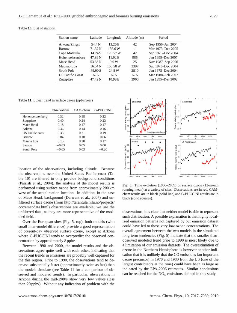
Observations of surface ozone over the last decades indi-cate a significant rise in the Northern Hemisphere (Parrishet al., 2004; Oltmans et al., 2006; Derwent et al., 2007).We focus here on stations with at least 20 years of observa-tions (Table 10), providing timeseries for comparison withmodel results. Model ozone fields are interpolated to the



Table 10.List of stations.

Station name Latitude Longitude Altitude (m) Period

Arkona/Zingst 54.4 N 13.26 E 42 Sep 1956–Jun 2004Barrow 71.32 N 156.6 W 11 Mar 1973–Dec 2005Cape Matatula 14.24 S 170.57 W 42 Sep 1975–Dec 2004Hohenpeissenberg 47.89 N 11.02 E 985 Jan 1995–Dec 2007Mace Head 53.33 N 9.9 W 25 Nov 1987–Sep 2006Maunao Loa 16.54 N 155.58 W 3397 Sep 1973–Dec 2004South Pole 89.90 S 24.8 W 2810 Jan 1975–Dec 2004US Pacific Coast N/A N/A N/A Mar 1988–Feb 2007Zugspitze 47.42 N 10.98 E 2960 Jan 1995–Dec 2002

Table 11.Linear trend in surface ozone (ppbv/year)

Observations CAM-chem G-PUCCINI

Hohenpeissenberg 0.32 0.18 0.22Zugspitze 0.40 0.24 0.23Mace Head 0.18 0.17 0.17Arkona 0.36 0.14 0.16US Pacific coast 0.33 0.21 0.19Barrow 0.04 0.10 0.06Mauna Loa 0.15 0.28 0.17Samoa −0.03 0.05 0.00South Pole −0.05 0.03 −0.20

location of the observations, including altitude. Becausethe observations over the United States Pacific coast (Ta-ble 10) are filtered to only provide background conditions(Parrish et al., 2004), the analysis of the model results isperformed using surface ozone from approximately 200 kmwest of the actual station location. In addition, in the caseof Mace Head, background (Derwent et al., 2007) and un-filtered surface ozone (fromhttp://tarantula.nilu.no/projects/ccc/emepdata.html) observations are available; we use theunfiltered data, as they are more representative of the mod-eled field.

Over the European sites (Fig. 5, top), both models (withsmall inter-model difference) provide a good representationof present-day observed surface ozone, except at Arkonawhere G-PUCCINI tends to overpredict the observed con-centration by approximately 8 ppbv.

Between 1990 and 2000, the model results and the ob-servations agree quite well with each other, indicating thatthe recent trends in emissions are probably well captured forthe this region. Prior to 1990, the observations tend to de-crease substantially faster (approximately twice as fast) thanthe models simulate (see Table 11 for a comparison of ob-served and modeled trends). In particular, observations inArkona during the mid-1980s show very low values (lessthan 20 ppbv). Without any indication of problem with the

Ozo

ne

mix

ing

rati

o (p

pb

v)O

zon

e m

ixin

g ra

tio

(pp

bv)

Ozo

ne

mix

ing

rati

o (p

pb

v)O

zon

e m

ixin

g ra

tio

(pp

bv)

Hohenpeissenberg

Zugspitze Mace Head

Arkona US Pacific coast

Fig. 5. Time evolution (1960–2009) of surface ozone (12-monthrunning mean) at a variety of sites. Observations are in red, CAM-chem results are in black (solid line) and G-PUCCINI results are inblack (solid squares).

observations, it is clear that neither model is able to representsuch distribution. A possible explanation is that highly local-ized emission patterns not captured by our emission datasetcould have led to those very low ozone concentrations. Theoverall agreement between the two models in the simulatedlong-term tendencies (Fig. 5) indicate that the smaller-than-observed modeled trend prior to 1990 is most likely due toa limitation of our emission datasets. The overestimation ofozone in the Northern Hemisphere is however another indi-cation that it is unlikely that the CO emissions (an importantozone precursor) in 1970 and 1980 from the US (one of thelargest contributors at the time) could have been as large asindicated by the EPA-2006 estimates. Similar conclusionscan be reached for the NOx emissions defined in this study.


http://tarantula.nilu.no/projects/ccc/emepdata.html


7030 J.-F. Lamarque et al.: 1850–2000 gridded anthropogenic and biomass burning emissionsO

zon

e m

ixin

g ra

tio

(pp

bv)

Barrow

Ozo

ne

mix

ing

rati

o (p

pb

v)

Mauna Loa

Ozo

ne

mix

ing

rati

o (p

pb

v)

Samoa South Pole

Ozo

ne

mix

ing

rati

o (p

pb

v)

Fig. 6. Time evolution (1970–2009) of surface ozone (12-monthrunning mean) at a variety of sites. Observations are in red, CAM-chem results are in black (solid line) and G-PUCCINI results are inblack (solid squares). A constant value of 6 ppbv was added to theBarrow observations to take into account model deficiencies; this isshown as green dots.

Over the US Pacific Coast, the models are again quite sim-ilar to one another, but neither matches the rapid increase insurface ozone seen in observations in recent years (Parrish etal., 2004).

However, additional long-term records of surface ozone(Barrow, Alaska; Mauna Loa, Hawaii; Cape Matatula, Amer-ican Samoa; South Pole, Antarctica, Fig. 6) show a differentpicture, in which changes in ozone in the 1980s are not in-creasing as rapidly, if at all. In particular, the record at Samoaactually indicates a long-term decrease in ozone, contrary tothe findings of Lelieved et al. (2004). In all those places,both models perform quite well in their capture of the long-term trends (note that, for visualization purposes, a constantbias of 6 ppbv was added to the observed record at Barrowto match the simulated levels; this is likely due to the spe-cific environment at Barrow, at the edge of the Arctic Ocean,which is difficult to capture with a coarse-grid global model).At Samoa, climate trends may have played a substantial rolein the apparent decrease between∼1990 and∼2000 in theobservations, as the models have rather different trends de-spite the same emissions data. The use of observed SSTs inthe G-PUCCINI simulations may have allowed it to capturelocal climate changes that could have contributed to the re-cent ozone decline seen in that remote Western Pacific lo-cation. At the South Pole, there is indication of the im-pact of stratospheric ozone depletion, bringing minimal lev-els during the mid-1990s, followed by a slight recovery andleveling-off since 2000 (Chipperfield et al., 2007). CAM-

chem is better able to capture this trend (Table 11), while G-PUCCINI tends to underestimate ozone in 2000, apparentlydue to an overestimate of downward transport of air havingexperienced Antarctic stratospheric ozone depletion (unlikethe surface, stratospheric ozone did not recover to the valuesseen in the 1970s and early 1980s by 2000; Chipperfield etal., 2007).

Neither model is capable of reproducing the Montsourisrecord (Volz and Kley, 1988), similar to the results of Lamar-que et al. (2005) and references therein. On the other hand,in terms of tropospheric ozone change (surface to 200 hPa),we find a very good agreement with the results of Gauss etal. (2006) with an increase of approximately 9 DU between1850 and 2000.

5.2.2 Surface carbon monoxide

Comparison (Fig. 7) of modeled and observed (averaged1990s conditions) surface carbon monoxide at Mace Head(a useful comparison since this station also provides sur-face ozone, Fig. 5) indicates a negative bias (approximately20 ppbv) and a somewhat reduced seasonal cycle, with alarger negative bias during winter. These features are presentin both simulations and are found at most of the NorthernHemisphere stations (not shown); agreement during summerconditions seems to always be slightly better than in the win-ter. Biases in the Southern Hemisphere are much smaller (es-pecially for CAM-chem, not shown). The overall NorthernHemisphere negative bias in both model simulations pointstowards an underestimation of the carbon monoxide (andpossibly NMVOCs) in our dataset; however, comparisonwith other published estimates (Table 5) does not indicate aclear negative bias in either anthropogenic or biomass burn-ing emissions of carbon monoxide. Owing to the long life-time of carbon monoxide during winter (up to a few months;Edwards et al., 2005), it is possible that biomass burningemissions in the latter part of the year over Russia are notwell enough characterized to provide the wintertime maxi-mum (Edwards et al., 2005). But, further analysis (beyondthe scope of this paper) is required to fully understand thereason for this low bias.

The long-term change (between 1990 and present, Fig. 8)in carbon monoxide at Mace Head (using unfiltered obser-vations, seehttp://tarantula.nilu.no/projects/ccc/emepdata.html) shows that the models capture the recent change rela-tively well; it is clear however that this analysis suffers fromthe lack of long-term (>10 years) records. Interestingly, thesimulated change in surface CO at Mace Head between 1960and 1990 is quite different between the two models, muchmore so than the ozone change over the same period.

The lifetimes of CO and CH4 can be used as global mea-sures of the OH content of the atmosphere. For the 2000 con-ditions, the methane chemical lifetime (i.e. not including thesmall deposition flux as the simulations were performed withspecified bottom layer methane concentration) is 8.9 years





Mace HeadC

O c

on

cen

trat

ion

(pp

bv)

Fig. 7. Seasonal cycle of carbon monoxide (ppbv) at Mace Head forthe 1990s. Observations (averaged 1991–1999) are in red, CAM-chem results are in black (solid line) and G-PUCCINI results are inblack (solid squares).

for CAM-chem and 8.6 years for G-PUCCINI, in excellentagreement with the IPCC AR-4 estimates of 8.7±1.3 years(Denman et al., 2007). For the same period, the CO life-time is 1.7 months for CAM-chem, in good agreement withHorowitz et al. (2003). There is therefore no indication that asignificant bias in OH in our model simulations could explainthe low bias in CO.

5.2.3 Mid- and upper-tropospheric ozone

A compilation of mid-tropospheric ozone observations froma variety of platforms (Cooper et al., 2010) indicates thatWestern United North America (25◦–55◦ N, 130◦–90◦ W,3–8 km) has experienced a recent (1995–2008) increase inozone concentration (Fig. 9), most likely associated withAsian emissions. The model results indicate again thatthey are performing very well in estimating the present-day(2000) ozone concentration. Evidently, they are not able toreproduce inter-annual variability but our 5- to 10-yr aver-ages are close to the observed values. Similarly to Fig. 5,the two models exhibit a consistent long-term evolution. Thsobservational dataset provides a much lower 1980s ozoneconcentration than the models indicate, similar to the surfaceozone analysis above.

5.2.4 Aerosol optical depth, burden and lifetime

A useful measure of the radiative impact of aerosols can beevaluated through the calculation of the aerosol optical depth(Schulz et al., 2006). We display in Fig. 10 the CAM-chemsimulated annual average total aerosol optical depth (AOD)at 550 nm for 1850 and 2000. The occurrence of widespreadpollution over the Northern Hemisphere is clearly identifi-able. In terms of the global average, the 2000 AOD sim-

CO

mix

ing

rati

o (p

pb

v)

Fig. 8. Time evolution (1960–2009) of surface CO (12-month run-ning mean) at Mace Head. Observations are in red, CAM-chemresults are in black (solid line) and GPUCCINI results are in black(solid squares). A constant value of 25 ppbv was subtracted from theobservations to take into account model deficiencies; this is shownas green dots.

ulated value is 0.12, which represents an increase of 0.033over the 1850 conditions (0.087). This anthropogenic in-crease is very much in agreement with the average AeroComresults (Schulz et al., 2006). We also compare our annualaverage aerosol optical depths to AERONET sun photome-ter site data at 173 sites globally (Holben, et al., 1998). Sunphotometry data represents some of the highest quality datafor assessing total aerosol optical depth. We include all sta-tions where monthly averages at 500 nm were available forall 12 months. The model is able to capture much of thevariability, but underestimates the aerosols optical depth athigh observed values (Fig. 11). The correlation coefficientbetween modeled values and observations is 0.67. In terms ofdust and sea-salt aerosols, comparison with surface observa-tions (using iron deposition as a proxy, see Fig. 12) indicatesa reasonable representation of present-day conditions.

An additional important evaluation for aerosol is theirglobal burden and lifetime. Results for the 2000 condi-tions are summarized in Table 6. Compared to the Aero-Com results (Schulz et al., 2006), the lifetime of carbona-ceous aerosols is approximately 2 days shorter (from approx-imately 7.5 days to 5.5 days), leading to a smaller burden. Onthe other hand, sulfate lifetime is almost exactly the same, asis the anthropogenic contribution (i.e. the difference between2000 and 1850 burdens).

5.2.5 Aerosol ice-core deposition

Ice core measurement of aerosol and gas content can provideinformation on long-term changes in deposition and con-centration. In particular, Greenland ice cores have been re-cently used to study the importance of black carbon in the



Ozo

ne

mix

ing

rati

o (p

pb

v)

Fig. 9. Time evolution (1970–2009) of mid-troposphere ozone(springtime mean) from Cooper et al. (2010). Observations are inred, CAM-chem results are in black (solid line) and G-PUCCINIresults are in black (solid squares).

1850

2000

Fig. 10. Total (natural and anthropogenic) CAM-chem simulatedaerosol optical depth at 550 nm (decadal average) for 1850 and2000.

Arctic (McConnell et al., 2007). The model results (wetand dry deposition of sulfate and black carbon) are inter-polated to the model grid point nearest to the D4 ice coresite (71.4◦ N, 44◦ W) with the closest model topography al-titude to D4 (approx. 100 km north of the actual D4 loca-

Fig. 11. Comparison between observed and modeled (present-day)annually aerosol optical depth at 500 nm. The observed values arebased on annually averaged AERONET optical depths (Holben etal., 1998).

tion); indeed, precipitation patterns (and therefore deposi-tion) exhibit a strongly decreasing latitudinal gradient acrossthe Greenland ice sheet. There is a remarkable agreement(Fig. 13, top) between the observations and the simulated de-position. In terms of sulfate, the maximum deposition rate(40 mg/m2/year in the observations) occurs in 1980, whenthe global emissions (but especially over the United Statesand Russia) peaked (Fig. 2). There is also indication of alocal maximum sulfate deposition at the beginning of the20th century in both the observations and the model field.

Similarly (Fig. 13, bottom), black carbon (hydrophiliconly) deposition at D4 has peaked in the early part of the20th century. We find that, using the same sampling proce-dure as for sulfate, the model captures that feature quite well(albeit not as strongly as the observations suggest), alongwith the overall changes over the simulated period. Thisis again indicative of adequate regional emission changes inNorth America as Greenland deposition is most strongly in-fluenced by emissions in that region (Shindell et al., 2008), inthis case related to changes (in both anthropogenic emissionsincreasing, see Fig. 2) and biomass burning (decreasing, seeFig. 3).

6 Discussion and conclusions

We have presented in this paper a dataset of historical an-thropogenic (defined here as originating from industrial, do-mestic and agriculture activity sectors) and biomass burn-ing emissions of reactive gases and aerosols covering 1850–2000. This dataset builds upon and complements previousinventories. In particular, our dataset represents a combi-nation of existing regional and global inventories (Table 4),



10-5 10-4 10-3 10-2 10-1 100 101 102

Obs g/m2/yr

10-5

10-4

10-3

10-2

10-1

100

101

102

Mod

el g

/m2/

yr

North AmericaNorth AtlanticSouth America, Africa and Atlantic

EuropeNorth Pacific/Asia/N. IndianS. Pacific/S. Indian

Fig. 12. Comparison between observed and modeled (present-day) iron concentration at a variety of sites (g/m2/year). The compiledobservations are available from Mahowald, et al. (2009).

Sulfa

te d

epo

siti

on

(mg

/m2/

year

)B

lack

car

bo

n d

epo

siti

on

(mg

/m2/

year

)

Fig. 13. Deposition (annual average) over Greenland (D4 site)of sulfate and black carbon. Ice-core observations are in red andCAM-chem results are in black.

and the combination of information was performed on aregional (40 regions) and sectoral (12 sectors) represen-tation (Tables 2 and 3). Of course, the use of a vari-ety of inventories precludes full consistency between car-

Table 12. Global burden and lifetime for anthropogenically-perturbed aerosols in 1850 and 2000 for the CAM-chem simulation.

1850 2000

Sulfate

Burden (mg(SO4)/m2) 1.55 3.65Lifetime (days) 3.4 3.6

Black carbon

Burden (mg(C)/m2) 0.09 0.24Lifetime (days) 5.6 5.8

Organic carbon

Burden (mg(C)/m2) 0.64 1.04Lifetime (days) 5.2 5.4

bon dioxide, reactive gases and aerosol emissions for an-thropogenic, biomass burning, land-use and natural emis-sions. It is unclear how important this lack of full con-sistency is, but it will be important to focus on this issuein future similar emission datasets. All data are publiclyavailable athttp://www.iiasa.ac.at/web-apps/tnt/RcpDbandftp://ftp-ipcc.fz-juelich.de/pub/emissions/.

The primary purpose of this inventory is to provideemissions for chemistry-climate simulations (with the Cli-mate Model Intercomparison Program #5 in support of theIPCC AR5 as the overall focus) for the study of long-termchanges in atmospheric composition. In particular, the emis-sions for year 2000 serve as an anchor point for historicalemissions (as discussed in this paper) and future emissions(as will be discussed in separate publications). This en-sures continuity in emission datasets throughout the periodof interest (1850–2100). Because of its focus on long-term


http://www.iiasa.ac.at/web-apps/tnt/RcpDb

ftp://ftp-ipcc.fz-juelich.de/pub/emissions/


changes, this dataset provides emissions every 10 years anddoes not attempt to reproduce interannual variability, whichcan be significant, particularly for biomass burning emis-sions.

Based on the recent studies by Bond et al. (2004, 2007)and Smith et al. (2010) uncertainties in regional emissionscan be expected to be as large as a factor of 2 (or even larger).The comparison of our year 2000 emissions with publishedestimates does not indicate significant biases (Table 5). How-ever, large differences with the EPA-2006 estimates of theUS. CO emissions for 1970 and 1980 are found (Table 6),with the possible explanation that those EPA estimates arethemselves strongly overestimated (Parrish, 2006). Otherspecies display a smaller spread amongst estimates and ourdataset tends to fall within the range of published estimates.

Using two chemistry-climate models, we have performed1850–2000 simulations (transient or time-slice experiments)in order to provide a first-order evaluation of the emissions.The focus of this evaluation is on long-term changes of tro-pospheric species relevant to climate forcing. In particular,we find that the model simulations for the 1990–2000 con-ditions represent quite well the observed surface and mid-troposphere ozone distributions. There is however indicationthat the modeled long-term increase since the early 1980s isnot as strong and rapid as recent publications indicate (Par-rish et al., 2004; Cooper et al., 2010), at least in the North-ern mid-latitudes. Indeed, comparison with other long-termozone records (Barrow, Mauna Loa, Samoa and South Pole)shows good agreement for the available period 1970–2000;there is therefore clearly a need for understanding ozonechanges at the regional scale. We found that, in our simu-lations, carbon monoxide is biased low in both models; thereason for this bias (present in many sites over the NorthernHemisphere but not so much in the Southern Hemisphere) isnot clear at this point.

Ice-core deposition of sulfate and black carbon overGreenland is well simulated (albeit only the CAM-chemmodel has simulated aerosols) in both amplitude and long-term trend. In particular, the black carbon maximum at theturn of the 20th century is a combination of increasing an-thropogenic and decreasing biomass burning emissions. Inaddition, global measures of aerosol content are inline withthe AeroCom estimates (Schulz et al., 2006) for present-dayburden and lifetime, especially for sulfate. Finally, aerosoloptical depth comparison with AERONET observations in-dicates a reasonably good simulation of present-day condi-tions.

The observations of long-term changes in atmosphericcomposition clearly indicate large regional variations. Asdiscussed in our paper, modeling these changes is a difficultchallenge that combines the role of changing emissions andchanging climate.

The dataset and simulations discussed here have in par-ticular shown the continuing underestimate of the long-termtrends in surface and mid-troposphere ozone, especially for

the continuous surface records from as early as the 1970sfor several stations. Similar to the Montsouris early 1900sobservations (Volz and Kley, 1988), the simulation of thefull amplitude of those observed trends remains problematic,possibly highlighting limits in our present understanding oftropospheric ozone.

Acknowledgements.The authors would like to thank the ACCENTEuropean Network, which provided funding for meetings todevelop the emissions dataset. Suvi Monni, Lorenzo Orlandiniand Valerio Pagliari are acknowledged for providing support in thegridding of emissions and making available official reported datafrom EMEP and UNFCCC inventories. O. Buhaug and J. Corbettprovided helpful comments on ship emissions. Z. K. would like toacknowledge the support received from the European Integratedproject on Aerosol Cloud Climate and Air Quality Interactions(EUCAARI), a project within EU’s Sixth Framework Program.A.H. acknowledges funding from the European Union’s CITYZENproject. Surface data was obtained from the World Data Centre forGreenhouse gases, maintained by the Japan Meteorological Agencyin cooperation with the World Meteorological Organization. Wewould like to thank D. Parrish and H.-E. Scheel for providingaccess to their ozone datasets. AERONET data was kindly madeavailable by the AERONET investigators and used for this study.The National Center for Atmospheric Research is operated bythe University Corporation for Atmospheric Research undersponsorship of the National Science Foundation. Any opinions,findings and conclusions or recommendations expressed in thepublication are those of the author(s) and do not necessarily reflectthe views of the National Science Foundation.

Edited by: R. Harley

References

Andreae, M. O. and Merlet, P.: Emission of trace gases and aerosolsfrom biomass burning, Global Biogeochem. Cy., 15, 955–966,2001.

Andres, R. J., Fielding, D. J., Marland, G., Boden, T. A., Kumar,N.: Carbon dioxide emissions from fossil-fuel use, 1751–1950,Tellus, 51, 759–765, 1999.

Beusen, A. H. W., Bouwman, A. F., Heuberger, P. S. C., Van Drecht,G., and Van Der Hoek, K. W.: Bottom-up uncertainty estimatesof global ammonia emissions from global agricultural productionsystems, Atmos. Environ., 42(24), 6067–6077, 2008.

Bian, H. and Prather, M.: Fast-j2: Accurate simulations of photol-ysis in global climate models, J. Atmos. Chem., 41, 281–296,2002.

Bond, T. C., Streets, D. G., Yarber, K. F., Nelson, S. M., Woo, J.-H.,Klimont, Z.: A Technology-Based Global Inventory of Black andOrganic Carbon Emissions from Combustion, J Geophys. Res.,109, D14203, doi:10.1029/2003JD003697, 2004.

Bond, T. C., Bhardwaj, E., Dong, R., Jogani, R., Jung, S., Ro-den, C., Streets, D. G., and Trautmann, N. M.: Historical emis-sions of black and organic carbon aerosol from energy-relatedcombustion, 1850–2000, Global Biogeochem. Cy., 21, GB2018,doi:10.1029/2006GB002840, 2007.

Buhaug, Ø., Corbett, J. J., Endresen, Ø., Eyring, V., Faber, J.,Hanayama, S., Lee, D. S., Lindstad, H., Mjelde, A., Palsson,



C., Wanquing, W., Winebrake, J. J., and Yoshida, K.: UpdatedStudy on Greenhouse Gas Emissions from Ships: Phase I Re-port; International Maritime Organization (IMO) London, UK,1 September 2008, p. 129, 2008.

Butkovskaya, N., Kukui, A., and Le Bras, G.: HNO3 forming chan-nel of the HO2+NO reaction as a function of pressure and tem-perature in the ranges of 72–600 torr and 223–323 k, J. Phys.Chem. A, 111, 9047–9053, 2007.

Chen, Y., Sheng, G., Bi, X., Feng, Y., Mai, B., and Fu, J.: Emissionfactors for carbonaceous particles and polycyclic aromatic hy-drocarbons from residential coal combustion in China, Environ.Sci. Tech., 39, 1861–1867, 2005.

Chen, Y., Zhi, G., Feng, Y., Fu, J., Feng, J., Sheng, G.,and Simoneit, B. R. T.: Measurements of emission fac-tors for primary carbonaceous particles from residential raw-coal combustion in China, Geophys. Res. Lett., 33, L20815,doi:10.1029/2006GL026966, 2006.

Charlton-Perez, C. L., Evans, M. J., Marsham, J. H., and Es-ler, J. G.: The impact of resolution on ship plume simula-tions with NOx chemistry, Atmos. Chem. Phys., 9, 7505–7518,doi:10.5194/acp-9-7505-2009, 2009.

Chipperfield, M. P., Fioletov, V. E., Bregman, B., Burrows, J., Con-nor, B. J., Haigh, J. D., Harris, N. R. P., Hauchecorne, A., Hood,L. L., Kawa, S. R., Krzy’scin, J. W., Logan, J. A., Muthama, N.J., Polvani, L., Randel, W. J., Sasaki, T., Stahelin, J., Stolarski, R.S., Thomason, L. W., and Zawodny, J. M.: Global Ozone, 2007:Past and Present, Chapter 3 in Scientific Assessment of OzoneDepletion: 2006, World Meteorological Organization, Geneva,Switzerland, Global Ozone Research and Monitoring Project –Report No. 50, 572 pp., 2006.

Christian, T. J., Kleiss, B., Yokelson, R. J., Holzinger, R., Crutzen,P. J., Hao, W. M., Saharjo, B. H., and Ward, D. E.: Compre-hensive laboratory measurements of biomass-burning emissions:1. Emissions from Indonesian, African, and other fuels, J. Geo-phys. Res., 108, 4719, doi:10.1029/2003JD003704, 2003.

Clarke, L., Edmonds, J., Jacoby, H., Pitcher, H., Reilly, J., andRichels, R.: Scenarios of Greenhouse Gas Emissions and At-mospheric Concentrations, Sub-report 2.1: A of Synthesis andAssessment Product 2.1 by the US Climate Change Science Pro-gram and the Subcommittee on Global Change Research. De-partment of Energy, Office of Biological & Environmental Re-search, Washington, DC., USA, 154 pp., 2007.

Cofala, J., Amann, M., Klimont, Z., Kupiainen, K., and Hoglund-Isaksson, L.: Scenarios of Global Anthropogenic Emissions ofAir Pollutants and Methane until 2030, Atmos. Environ., 41,8486–8499, doi:10.1016/j.atmosenv.2007.07.010, 2007.

Cooper, O. R., Parrish, D. D., Stohl, A., Trainer, M., Nedelec, P.,Thouret, V., Cammas, J. P., Oltmans, S. J., Johnson, B. J., Tara-sick, D., Leblanc, T., McDermid, I. S., Jaffe, D., Gao, R., Stith,J., Ryerson, T., Aikin, K., Campos, T., Weinheimer, A., and Av-ery, M. A.: Increasing springtime ozone mixing ratios in the freetroposphere over western North America, Nature, 463, 344–348,doi:10.1038/nature08708, 2010.

Corbett, J. J. and Kohler, H. W.: Updated emissionsfrom ocean shipping, J. Geophys. Res., 108, 4650,doi:10.1029/2003JD003751, 2003.

Dentener, F., Drevet, J., Lamarque, J.-F., et al.: Nitrogen andSulphur Deposition on regional and global scales: a multi-model evaluation, Global Biogeochem. Cy., 20, GB4003,

doi:10.1029/2005GB002672, 2006.Denman, K. L., Brasseur, G., Chidthaisong, A., Ciais, P., Cox, P.

M., Dickinson, R. E., Hauglustaine, D., Heinze, C., Holland, E.,Jacob, D., Lohmann, U., Ramachandran, S., da Silva Dias, P. L.,Wofsy, S. C., and Zhang, X.: Couplings Between Changes in theClimate System and Biogeochemistry, in: Climate Change 2007:The Physical Science Basis. Contribution of Working Group Ito the Fourth Assessment Report of the Intergovernmental Panelon Climate Change, edited by: Solomon, S., Qin, D., Manning,M., Chen, Z., Marquis, M., Averyt, K. B., Tignor, M., and Miller,H. L., Cambridge University Press, Cambridge, United Kingdomand New York, NY, USA, 2007.

Derwent, R. G., Simmonds, P. G., Manning, A. J., and Spain, T. G.:Trends over a 20-year period from 1987 to 2007 in surface ozoneat the atmospheric research station, Mace Head, Ireland, Atmos.Environ., 41, 9091–9098, 2007.

Duncan, B. N., Martin, R., Staudt, A., Yevich, R., and Logan, J.:Interannual and Seasonal Variability of Biomass Burning Emis-sions Constrained by Satellite Observations, J. Geophys. Res.,108(D2), 4100, doi:10.1029/2002JD002378, 2003.

EMEP: Inventory Review 2006: Emission data reported to the LR-TAP Convention and NEC Directive, Stage 1, 2 and 3 review,Evaluation of inventories of HMs and POPs, edited by: Vestreng,V., Rigler, E., Adams, M., et al., EMEP MSC-W, Oslo, Norway,2006.

Endresen, Ø., Sørgard, E., Sundet, J. K., Dalsøren, S. B., Isaksen, I.S. A., Berglen, T. F., and Gravir, G.: Emission from internationalsea transportation and environmental impact, J. Geophys. Res.,108, 4560, doi:10.1029/2002JD002898, 2003.

Endresen, Ø., Sørgard, E., Behrens, H. L., Brett, P. O., andIsaksen, I. S. A.: A historical reconstruction of ships’ fuelconsumption and emissions, J. Geophys. Res., 112, D12301,doi:10.1029/2006JD007630, 2007.

Erisman, J. W., Sutton, M. A., Galloway, J., Klimont, Z., and Wini-warter, W.: How a century of ammonia synthesis changed theworld, Nat. Geosci., 1(10), 636–639, 2009.

European Commission: Joint Research Centre (JRC)/NetherlandsEnvironmental Assessment Agency (PBL), Emission Databasefor Global Atmospheric Research (EDGAR), release version 4.0.http://edgar.jrc.ec.europa.eu(last access: 16 February 2010),2009.

Eyers, C. J., Addleton, D., Atkinson, K., Broomhead, M. J., Chris-tou, R., Elliff, T., Falk, R., Gee, I., Lee, D. S., Marizy, C., Michot,S., Middel, J., Newton, P., Norman, P., Plohr, M., Raper, D., andStanciou, N.: AERO2K global aviation emissions inventories for2002 and 2025, QINETIQ/04/01113, 2005.

Eyring, V., Kohler, H. W., van Aardenne, J., and Lauer, A.: Emis-sions from International Shipping: 1. The last 50 Years, J. Geo-phys. Res., 110, D17305, doi:10.1029/2004JD005619, 2005.

Eyring, V., Isaksen, I. S. A., Berntsen, T., Collins, W. J.,Corbett, J. J., Endresen, O., Grainger, R. G., Moldanova,J., Schlager, H., and Stevenson, D. S.: Transport im-pacts on atmosphere and climate: Shipping, Atmos. Environ.,doi:10.1016/j.atmosenv.2009.04.059, in press, 2010.

FAO (Food and Agriculture Organization): WRB (World ReferenceBase) Map of World Soil Resources. Land and Water Develop-ment Division AGL,http://www.fao.org/ag/agl/agll/wrb/soilres.stm, last access: 16 February 2010, Food and Agriculture Orga-nization of the United Nations, Rome, Italy, 2003.


http://edgar.jrc.ec.europa.eu

http://www.fao.org/ag/agl/agll/wrb/soilres.stm

http://www.fao.org/ag/agl/agll/wrb/soilres.stm


Fernandes, S. M., Trautmann, N. M., Streets, D. G., Roden, C. A.,and Bond, T. C.: Global biofuel use, 1850–2000, Global Bio-geochem. Cy., 21, GB2019, doi:10.1029/2006GB002836, 2007.

Franke, K., Eyring, V., Sander, R., Hendricks, J., Lauer, A., andSausen, R.: Toward Effective Emissions of Ships in Global Mod-els, Meteorol. Z., 17(2), 117–129, 2008.

Fujino, J., Nair, R., Kainuma, M., Masui, T., and Matsuoka, Y.:Multigas mitigation analysis on stabilization scenarios usingAIM global model, Multigas Mitigation and Climate Policy, TheEnergy Journal Special Issue, 343–354, 2006.

Garg, A., Shukla, P. R., and Kapshe, M.: The sectoral trendsof multigas emissions inventory of India, Atmos. Environ. 40,4608–4620, 2006.

Gauss, M., Myhre, G., Isaksen, I. S. A., Grewe, V., Pitari, G., Wild,O., Collins, W. J., Dentener, F. J., Ellingsen, K., Gohar, L. K.,Hauglustaine, D. A., Iachetti, D., Lamarque, F., Mancini, E.,Mickley, L. J., Prather, M. J., Pyle, J. A., Sanderson, M. G.,Shine, K. P., Stevenson, D. S., Sudo, K., Szopa, S., and Zeng, G.:Radiative forcing since preindustrial times due to ozone changein the troposphere and the lower stratosphere, Atmos. Chem.Phys., 6, 575–599, doi:10.5194/acp-6-575-2006, 2006.

Gent, P. R., Yeager, S. G., Neale, R. B., Levis, S., and Bailey, D.A.: Improvements in a half degree atmosphere/land version ofthe CCSM, Clim. Dynam., 79, 25–58, doi:10.1007/s00382-009-0614-8, 2009.

Goldewijk, K.: Three centuries of global population growth:A spatial referenced population density database for 1700–2000, available athttp://www.mnp.nl/edgar/model/edgarv32/v32ftmaps/(last access: 16 February 2010), Popul. Environ.,26(5), 343–367, 2005.

Hanson, D. and Mauersberger, K.: Laboratory studies of the ni-tric acid tridydrate: Implications for the south polar stratosphere,Geophys. Res. Lett., 15, 855–858, 1988.

Heil, A.: Indonesian Forest and Peat Fires: Emissions, Air Quality,and Human Health, Berichte zur Erdsystemforschung, 34, Max-Planck-Institute for Meteorology, Hamburg, Germany, 2007.

Hijioka, Y., Matsuoka, Y., Nishimoto, H., Masui, M., and Kainuma,M.: Global GHG emissions scenarios under GHG concentrationstabilization targets, J. Global Environ. Eng., 13, 97–108, 2008.

Holben, B. N., Eck, T. F., Slutsker, I., et al.: AERONET-A Feder-ated Instrument Network and Data Archive for Aerosol Charac-terization, 1998.

Horowitz, L. W., Walters, S., Mauzerall, D. L., Emmons, L. K.,Rasch, P. J., Granier, C., Tie, X. X., Lamarque, J.-F., Schultz, M.G., Tyndall, G. S., Orlando, J. J., and Brasseur, G. P.: A globalsimulation of tropospheric ozone and related tracers: Descrip-tion and evaluation of MOZART, version 2, J. Geophys. Res.,108(D24), 4784, doi:10.1029/2002JD002853, 2003.

Houweling, S., Dentener, F., and Lelieveld, J.: The im-pact of non-methane hydrocarbon compounds on tropo-spheric photochemistry, J. Geophys. Res., 103, 10673–10696,doi:10.1029/97JD03582, 1998.

Iinuma, Y., Brueggemann, E., Gnauk, T., Mueller, K., Andreae,M. O., Helas, G., Parmar, R., and Herrmann, H.: Source char-acterization of biomass burning particles: The combustion ofselected European conifers, African hardwood, savanna grass,and German and Indonesian peat, J. Geophys. Res., 112, 8209,doi:10.1029/2006JD007120, 2007.

Ito, A. and Penner, J. E.: Historical emissions of carbona-

ceous aerosols from biomass and fossil fuel burning for theperiod 1870–2000, Global Biogeochem. Cy., 19, GB2028,doi:10.1029/2004GB002374, 2005.

Johnson, M., Edwards, R., Frenk, C. A., and Masera, O.: In-field greenhouse gas emissions from cookstoves in rural Mexicanhouseholds, Atmos. Environ., 42, 1206–1222, 2008.

Junker, C. and Liousse, C.: A global emission inventory of car-bonaceous aerosol from historic records of fossil fuel and bio-fuel consumption for the period 18601997, Atmos. Chem. Phys.,8, 1195–1207, doi:10.5194/acp-8-1195-2008, 2008.

Kasischke, E. S., Hyer, E. J., Novelli, P. C., Bruhwiler, L. P., French,N. H. F., Sukhinin, A., Hewson, J. H., and Stocks, B. J.: Influ-ences of boreal fire emissions on Northern Hemisphere atmo-spheric carbon and carbon monoxide. Global Biogeochem. Cy.,19, GB1012, doi:10.1029/2004GB002300, 2005.

Kinnison, D. E., Brasseur, G. P., Walters, S., et al.: Sensitiv-ity of Chemical Tracers to Meteorological Parameters in theMOZART-3 Chemical Transport Model, J. Geophys. Res., 112,D20302, doi:10.1029/2006JD007879, 2007.

Klimont, Z., Cofala, J., Xing, J., Wei, W., Zhang, C., Wang, S.,Kejun, J., Bhandari, P., Mathura, R., Purohit, P., Rafaj, P., Cham-bers, A., Amann, M., and Hao, J.: Projections of SO2, NOx, andcarbonaceous aerosols emissions in Asia, Tellus, 61B, 602–617,doi:10.1111/j.1600-0889.2009.00428.x, 2009.

Klimont, Z. and Streets, D. G.: Emissions inventories and projec-tions for assessing hemispheric or intercontinental transport, in:Hemispheric transport of air pollution 2007, edited by: Keating,T. and Zuber, A., United Nations, Geneva, Atmospheric Pollu-tion Studies No. 16, ECE/EB.AIR/94, 2007.

Lack, D., Lerner, B., Granier, C., Baynard, T., Lovejoy, E., Massoli,P., Ravishankara, A. R., and Williams, E.: Light absorbing car-bon emissions from commercial shipping, Geophys. Res. Let.,35, L13815, doi:10.1029/2008GL033906, 2008.

Lamarque, J.-F., Hess, P., Emmons, L., Buja, L., Washing-ton, W., and Granier, C.: Tropospheric ozone evolution be-tween 1890 and 1990, J. Geophys. Res., 110(D8), D08304,doi:10.1029/2004JD005537, 2005.

Lamarque, J.-F., Kinnison, D. E., Hess, P. G., and Vitt, F.: Simu-lated lower stratospheric trends between 1970 and 2005: identi-fying the role of climate and composition changes, J. Geophys.Res., 113, D12301, doi:10.1029/2007JD009277, 2008.

Lavoue, D., Liousse, C., Cachier, H., and Goldammer, J.: Carbona-ceous aerosol source inventory for temperate and boreal fires, J.Geophys. Res., 105, 26871–26890, 2000.

Lecht, M.: Comparison of DLR Fuel Flow Method and the P3-T3Method for Cruise EINOX Prediction, ICAO/CAEP/WG3 Al-ternative Emissions Methodology Task Group, Boeing, Seattle,USA, 22–23 September, 1999.

Lee, D. S., Owen, B., Graham, A., Fichter, C., Lim, L. L., andDimitriu, D.: Allocation of International aviation emissions fromscheduled air traffic – present day and historical (Report 2 of 3),Manchester Metropolitan University, Centre for Air Transportand the Environment,http://www.cate.mmu.ac.uk/documents/projects/mmuallocationsreport2currentdayv15.pdf last access:(16 February 2010), Manchester, UK, CATE-2005-3(C)-2, 2005.

Lelieveld, J., van Aardenne, J., Fischer, H., de Reus, M., Williams,J., and Winkler, P: Increasing Ozone over the Atlantic Ocean,Science, 304, 1483, doi:10.1126/science.1096777, 2004.

Liao, H., Adams, P. J., Ching, S. H., et al.: Interactions be-


http://www.mnp.nl/edgar/model/edgarv32/v32ftmaps/

http://www.mnp.nl/edgar/model/edgarv32/v32ftmaps/

http://www.cate.mmu.ac.uk/ documents/projects/mmuallocationsreport2currentdayv1_5.pdf

http://www.cate.mmu.ac.uk/ documents/projects/mmuallocationsreport2currentdayv1_5.pdf


tween tropospheric chemistry and aerosols in a unified gen-eral circulation model, J. Geophys. Res., 108(D1), 4001,doi:10.1029/2001JD001260, 2003.

Mahowald, N., Muhs, D. R., Levis, S., et al.: Change in atmosphericmineral aerosols in response to climate: last glacial period, pre-industrial, modern and doubled-carbon dioxide climates, J. Geo-phys. Res., 111, D10202, doi:10210.11029/12005JD006653,2006a.

Mahowald, N., Lamarque, J.-F., Tie, X. X., and Wolff, E.: Seasalt aerosol response to climate change: last glacial maximum,pre-industrial,and doubled-carbon dioxide climates, J. Geophys.Res., 111, D05303, doi:10.1029/2005JD006459, 2006b.

Mahowald, N., Engelstaeder, S., Luo, C., et al.: Atmo-spheric Iron deposition: Global distribution, variability andhuman perturbations, Annu. Rev. Mar. Sci., 1, 245–278,doi:210.1146/annurev/marine.010908.163727, 2009.

Marlon, J. R., Bartlein, P. J., Carcaillet, C., Gavin, D. G., Har-rison, S. P., Higuera, P. E., Joss, F., Power, M. J., and Pren-tice, I. C.: Climate and human influences on global biomassburning over the past two millenia, Nat. Geosci., 1, 697–702,doi:10.1038/ngeo313, 2008.

McConnell, J. R., Edwards, R., Kok, G. L., Flanner, M. G., Zen-der, C. S., Saltzman, E. S., Banta, J. R., Pasteris, D. R., Carter,M. M., and Kahl, J. D. W.: 20th Century industrial black car-bon emissions altered Arctic climate forcing, Science, 317, 5843,doi:10.1126/science.1144856, 2007.

Meehl, G. A., Stocker, T. F., Collins, W. D., Friedlingstein, P., Gaye,A. T., Gregory, J. M., Kitoh, A., Knutti, R., Murphy, J. M., Noda,A., Raper, S. C. B., Watterson, I. G., Weaver, A. J., and Zhao,Z.-C.: Global Climate Projections, in: Climate Change 2007:The Physical Science Basis, Contribution of Working Group I tothe Fourth Assessment Report of the Intergovernmental Panel onClimate Change, edited by: Solomon, S., Qin, D., Manning, M.,Chen, Z., Marquis, M., Averyt, K. B., Tignor, M., and Miller, H.L., Cambridge University Press, Cambridge, UK and New York,NY, USA, 2007.

Metzger, S., Dentener, F., Pandis, S., and Lelieveld, J.: Gas/aerosolpartitioning: 1. A computationally efficient model, J. Geophys.Res., 107(D16), 4312, doi:10.1029/2001JD001102, 2002.

Mieville, A., Granier, C., Liousse, C., Guillaume, B., Mouillot, F.,Lamarque, J.-F., Gregoire, J.-M., and Petron, G.: Emissions ofgases and particles from biomass burning using satellite data andan historical reconstruction, Atmos. Environ., 44, 1469–1477,doi:10.1016/j.atmosenv.2010.01.011, 2010.

Moss, T., Babiker, M., Brinkman, S., Calvo, E., Carter, T., Ed-monds, J., Elgizouli, I., Emori, S., Erda, L., Hibbard, K., Jones,R., Kainuma, M., Kelleher, J., Lamarque, J.-F., Manning, M.,Matthews, B., Meehl, G., Meyer, L., Mitchell, J., Nakic’enovic’,N., O’Neill, B., Pichs, T., Riahi, K., Rose, S., Runci, P., Stouffer,R., van Vuuren, D., Weyant, J., Wilbanks, T., van Ypersele, J. P.,and Zurek, M.: Towards New Scenarios for Analysis of Emis-sions, Climate Change, Impacts, and Response Strategies, avail-able at:http://www.aimes.ucar.edu/docs/, last access: 16 Febru-ary 2010, Intergovernmental Panel on Climate Change, Geneva,132 pp., 2008.

Mouillot, F. and Field, C. B.: Fire history and the global car-bon budget: a 1◦×1◦ fire history reconstruction for the 20thcentury, Glob. Change Biol., 11, 398–420, doi:10.1111/j.1365-2486.2005.00920.x, 2005.

NARSTO: Improving emission inventories for effective air qual-ity management across North America, NARSTO,http://www.narsto.org/section.src?SID=8(last access: 16 Feburary 2010),2006.

Ohara, T., Akimoto, H., Kurokawa, J., Horii, N., Yamaji, K.,Yan, X., and Hayasaka, T.: An Asian emission inventory ofanthropogenic emission sources for the period 1980–2020, At-mos. Chem. Phys., 7, 4419–4444, doi:10.5194/acp-7-4419-2007,2007.

Olivier, J. G. J., Bouwman, A. F., Van der Maas, C. W. M.,Berdowski, J. J. M., Veldt, C., Bloos, J. P. J., Visschedijk, A.J. H., Zandveld, P. Y. J., and Haverlag, J. L.: Description ofEDGAR Version 2.0, A set of global emission inventories ofgreenhouse gases and ozone-depleting substances for all anthro-pogenic and most natural sources on a per country basis and on1×1 degree grid, RIVM/TNO report, 1996.

Olivier, J. G. J., Van Aardenne, J. A., Dentener, F., Ganzeveld, L.,Peters, J. A. H. W., et al.: Recent trends in global greenhouse gasemissions: regional trends and spatial distribution of key sources,in: Non-CO2 Greenhouse Gases (NCGG-4), coordinator: vanAmstel, A., Millpress, Rotterdam, ISBN 905966 043 9, 325–330,2005.

Oltmans, S. J., Lefohn, A. S., Harris, J. M., et al.: Long-termchanges in tropospheric ozone, Atmos. Environ., 40, 3156–3173,2006.

Page, S. E., Siegert, F., Rieley, J. O., Boehm, H.-D. V., Jaya, A., andLimin, S.: The amount of carbon release from peat and forestfires in Indonesia during 1997, Nature, 420, 61–65, 2002.

Parashar, D. C., Gadi, R., Mandal, T. K., and Mitra, A. P.: Car-bonaceous aerosol emissions from India, Atmos. Environ., 39,7861–7871, 2005.

Parrish, D. D.: Critical evaluation f US on-road vehicle emissioninventories, Atmos. Environ., 40, 2288–2300, 2006

Parrish, D. D., Dunlea, E. J., Atlas, E. L., et al.: Changes in thephotochemical environment of the temperate North Pacific tro-posphere in response to increased Asian emissions, J. Geophys.Res., 109, D23S18, doi:10.1029/2004JD004978, 2004.

Petzold, A., Hasselbach, J., Lauer, P., Baumann, R., Franke, K.,Gurk, C., Schlager, H., and Weingartner, E.: Experimental stud-ies on particle emissions from cruising ship, their characteris-tic properties, transformation and atmospheric lifetime in themarine boundary layer, Atmos. Chem. Phys., 8, 2387–2403,doi:10.5194/acp-8-2387-2008, 2008.

Prather, M. J.: Numerical advection by conservation of second-order moments, J. Geophys. Res., 91, 6671–6681, 1986.

Randerson, J. T., van der Werf, G. R., Collatz, G .J., Giglio, L.,Still, C. J., Kasibhatla, P., Miller, J. B., White, J. W. C., De-Fries, R. S., and Kasischke, E. S.: Fire emissions from C3 andC4 vegetation and their influence on interannual variability ofatmospheric CO2 and d13CO2, Global Biogeochem. Cy., 19,GB2019, doi:10.1029/2004GB002366, 2005.

Rayner, N. A., Parker, D. E., Horton, E. B., Folland, C. K., Alexan-der, L. V., Rowell, D. P., Kent, E. C., and Kaplan, A.: Globalanalyses of sea surface temperature, sea ice, and night marine airtemperature since the late nineteenth century, J. Geophys. Res.,108(D14), 4407, doi:10.1029/2002JD002670, 2003.

Riahi, K., Gruebler, A., and Nakicenovic, N.: Scenarios oflong-term socioeconomic and environmental development un-der climate stabilization. Greenhouse Gases – Integrated Assess-


http://www.aimes.ucar.edu/docs/

http://www.narsto.org/section.src?SID=8

http://www.narsto.org/section.src?SID=8


ment, Special Issue, Technol. Forecast. Soc., 74(7), 887–935,doi:10.1016/j.techfore.2006.05.026, 2007.

Richter, A., Burrows, J. P., Nuss, H., Granier, C., and Niemeier, U.:Increase in tropospheric nitrogen dioxide over China observedfrom space, Nature, 437(7055), 129–132, 2005.

Roden, C. A., Bond, T. C., Conway, S., and Pinel, A. B. O.: Emis-sion factors and real-time optical properties of particles emittedfrom traditional wood burning cookstoves, Environ. Sci. Tech-nol., 40, 6750–6757, 2006.

Roden, C. A., Bond, T. C., Conway, S., Pinel, A. B. O., MacCarty,N., and Still, D.: Laboratory and field investigations of partic-ulate and carbon monoxide emissions from traditional and im-proved cookstoves, Atmos. Environ., 43, 1170–1181, 2009.

Sander, S. P., Friedl, R. R., DeMore, W. B., et al: Chemical ki-netics and photochemical data for use in stratospheric modeling,eval. 13, JPL publ. 00-003, 2000.

Sander S. P., R. R. Friedl, A. R. Ravishankara, et al.: Chemical Ki-netics and Photochemical Data for Use in Atmospheric StudiesEvaluation Number 15, Publication 06-2, Jet Propulsion Labora-tory, Pasadena, CA, 2006.

Sausen, R. and Schumann, U.: Estimates of the climate response toaircraft CO2 and NOx emissions scenarios, Climatic Change, 44,27–58, 2000.

Schmidt, G. A., Ruedy, R., Hansen, J. E., Aleinov, I., Bell, N.,Bauer, M., Bauer, S., Cairns, B., Canuto, V., Cheng, Y., Del Ge-nio, A., Faluvegi, G., Friend, A. D., Hall, T. M., Hu, Y., Kelley,M., Kiang, N. Y., Koch, D., Lacis, A. A., Lerner, J., Lo, K. K.,Miller, R. L., Nazarenko, L., Oinas, V., Perlwitz, J., Perlwitz,J., Rind, D., Romanou, A., Russell, G. L., Sato, M., Shindell,D. T., Stone, P. H., Sun, S., Tausnev, N., Thresher, D., and Yao,M.-S.: Present day atmospheric simulations using giss modele:Comparison to in-situ, satellite and reanalysis data, J. Climate,19, 153–192, 2006.

Schultz, M. and Rast, S.: Emission datasets and methodologies forestimating emissions, available at:http://retro.enes.org(last ac-cess: 16 February 2010), RETRO Report D1-6,, 2007.

Schultz, M. G., Heil, A., Hoelzemann, J. J., Spessa, A.,Thonicke, K., Goldammer, J., Held, A. C., Pereira, J. M.,and van het Bolscher, M.: Global Wildland Fire Emissionsfrom 1960 to 2000, Global Biogeochem. Cyc., 22, GB2002,doi:10.1029/2007GB003031, 2008.

Shindell, D. T., Faluvegi, G., Stevenson, D. S., et al., Multi-modelsimulations of carbon monoxide: Comparison with observa-tions and projected near-future changes, J. Geophys. Res., 111,D19306, doi:10.1029/2006JD007100, 2006a.

Shindell, D. T., Faluvegi, G., Unger, N., Aguilar, E., Schmidt,G. A., Koch, D. M., Bauer, S. E., and Miller, R. L.: Simula-tions of preindustrial, present-day, and 2100 conditions in theNASA GISS composition and climate model G-PUCCINI, At-mos. Chem. Phys., 6, 4427–4459, doi:10.5194/acp-6-4427-2006,2006b.

Shindell, D. T., Chin, M., Dentener, F., Doherty, R. M., Faluvegi,G., Fiore, A. M., Hess, P., Koch, D. M., MacKenzie, I. A.,Sanderson, M. G., Schultz, M. G., Schulz, M., Stevenson, D.S., Teich, H., Textor, C., Wild, O., Bergmann, D. J., Bey, I.,Bian, H., Cuvelier, C., Duncan, B. N., Folberth, G., Horowitz, L.W., Jonson, J., Kaminski, J. W., Marmer, E., Park, R., Pringle,K. J., Schroeder, S., Szopa, S., Takemura, T., Zeng, G., Keat-ing, T. J., and Zuber, A.: A multi-model assessment of pollu-

tion transport to the Arctic, Atmos. Chem. Phys., 8, 5353–5372,doi:10.5194/acp-8-5353-2008, 2008.

Sinha, P., P.V. Hobbs, R.J. Yokelson, T.J. Christian, T.W. Kirchstet-ter, and R. Bruintjes, Emissions of trace gases and particles fromtwo ships in the southern Atlantic Ocean, Atmos. Environ., 37,2139–2148, 2003.

Simos, D.: PIANO: PIANO User’s Guide Version 4.0, Lissys Lim-ited, UK www.piano.aero(last access: 16 February 2010), 2004.

Smith, S. J., Steven, J., Pitcher, H., and Wigley, T. M. L.: Globaland Regional Anthropogenic Sulfur Dioxide Emissions, GlobalPlanet. Change, 29(1–2), 99–119, 2001.

Smith, S. J., Andres, R., Conception, E., and Lurz, J.: Histori-cal Sulfur Dioxide Emissions 1850–2000: Methods and Results,PNNL Research Report, Joint Global Change Research Institute,8400 Baltimore Avenue College park, Maryland, 20740, 2004.

Smith, S. J., van Aardenne, J., Klimont, Z., Andres, R., Volke,A., and Delgado Arias, S.: Anthropogenic sulfur dioxide emis-sions: 18502005, Atmos. Chem. Phys. Discuss., 10, 16111–16151, doi:10.5194/acpd-10-16111-2010, 2010.

Stevenson, D. S., Dentener, F. J., Schultz, M. G., et al.:Multi-model ensemble simulations of present-day and near-future tropospheric ozone, J. Geophys. Res., 111, D08301,doi:10.1029/2005JD006338, 2006.

Streets, D. G., Bond, T. M. L., Carmichael, G. R., Fernandes, S.,Fu, Q., He, D., Klimont, Z., Nelson, S. M., Tsai, N. Y., Wang, M.Q., Woo, J.-H., and Yarber, K. F.: An inventory of gaseous andprimary aerosol emissions in Asia in the year 2000. J. Geophys.Res., 108(D21), 8809, doi:10.1029/2002JD003093, 2003.

Streets, D. G., Zhang, Q., Wang, L., He, K., Hao, J., et al.: Re-visiting China’s CO emissions after the Transport and ChemicalEvolution over the Pacific (TRACE-P) mission: Synthesis of in-ventories, atmospheric modeling, and observations, J. Geophys.Res., 111, 1–16, 2006.

Taylor, K. E., Stouffer, R. J., and Meehl, G. A.: A Summary of theCMIP5 Experiment Design,https://cmip.llnl.gov/cmip5/docs/Taylor CMIP5 design.pdf(last access: 26 July 2010), 2009.

Tie, X. X., Brasseur, G. P., Emmons, L. K., et al.: Effects of aerosolson tropospheric oxidants: A global model study, J. Geophys.Res., 106, 2931–2964, 2001.

Tie, X. X., Madronich, S., Walters, S., et al.: Assessment of theglobal impact of aerosols on tropospheric oxidants, J. Geophys.Res., 110(D3), D03204, doi:10.1029/2004JD005359, 2005.

US Environmental Protection Agency: Compilation of air pollu-tant emission factors, US Environmental Protection Agency, Re-search Triangle Park, NC, 1996.

US Environmental Protection Agency: SPECIATE 4.0: Speciationdatabase development documentation, US Environmental Pro-tection Agency, Research Triangle Park, NC, 2006.

Van Aardenne, J. A., Dentener, F. J., Olivier, J. G. J., Klein Gold-ewijk, C. G. M., and Lelieveld, J.: A 1×1 degree resolutiondataset of historical anthropogenic trace gas emissions for theperiod 1890–1990, Global Biogeochem. Cy., 15(4), 909–928,2001.

Van Aardenne, J. A., Dentener, F., Olivier, J. G. J., and Pe-ters, J. A. H. W.: The EDGAR 3.2 Fast Track 2000 dataset(32FT2000), http://www.mnp.nl/edgar/model/v32ft2000edgar/docv32ft20(last access: 16 February 2010), 2005.

van der Werf, G. R., Randerson, J. T., Giglio, L., Collatz, G. J.,Kasibhatla, P. S., and Arellano Jr., A. F.: Interannual variabil-


http://retro.enes.org

www.piano.aero

https://cmip.llnl.gov/cmip5/docs/Taylor_CMIP5_design.pdf

https://cmip.llnl.gov/cmip5/docs/Taylor_CMIP5_design.pdf

http://www.mnp.nl/edgar/model/v32ft2000edgar/docv32ft20

http://www.mnp.nl/edgar/model/v32ft2000edgar/docv32ft20


ity in global biomass burning emissions from 1997 to 2004, At-mos. Chem. Phys., 6, 3423–3441, doi:10.5194/acp-6-3423-2006,2006.

Van Vuuren, D. P., Eickhout, B., Lucas, P. L., and den Elzen, M. G.J.: Long-term multi-gas scenarios to stabilise radiative forcing– Exploring costs and benefits within an integrated assessmentframework, Multigas Mitigation and Climate Policy, The EnergyJournal, Special Issue, 2006.

Van Vuuren, D. P., den Elzen, M. G. J., Lucas, P. L., Eickhout, B.,Strengers, B. J., van Ruijven, B., Wonink, S., and van Houdt,R.: Stabilizing greenhouse gas concentrations at low levels: anassessment of reduction strategies and costs, Climatic Change,81, 119–159, 2007.

Venkataraman, C., Habib, G., Eiguren-Fernandez, A., Miguel, A.H., and Friedlander, S. K.: Residential biofuels in South Asia:carbonaceous aerosol emissions and climate impacts, Science,307, 1454–1456, 2005.

Vestreng, V., Adams, M., and Goodwin, J.: Inventory review 2004,EMEP Techincal Report MSC-W1/2004, 2004.

Volckens, J., Olson, D. A., and Hays, M. D.: Carbonaceous speciesemitted from handheld two-stroke engines, Atmos. Environ., 42,1239–1248, 2008.

Volz, A. and Kley, D.: Ozone Measurements in the 19th Century:An Evaluation of the Montsouris Series, Nature, 332, 240–242,1988.

Wang, C., Corbett, J. J., and Firestone, J.: Improving Spatial Repre-sentation of Global Ship Emissions Inventories, ES&T, 42, 193–199, doi:10.1021/es0700799, 2007.

Yan, X., Akimoto, H., and Ohara, T.: Statistical modeling ofNOx emission from global soils, Global Biogeochem. Cy., 19,GB3019, doi:10.1029/2004GB002276, 2005.

Yevich, R. and J. A. Logan, An assesment of biofuel use and burn-ing of agricultural waste in the developing world, Global Bio-geochem. Cy., 17(4), 1095, doi:10.1029/2002GB001952, 2003.

Zhang, Q., Streets, D. G., Carmichael, G. R., He, K. B., Huo, H.,Kannari, A., Klimont, Z., Park, I. S., Reddy, S., Fu, J. S., Chen,D., Duan, L., Lei, Y., Wang, L. T., and Yao, Z. L.: Asian emis-sions in 2006 for the NASA INTEX-B mission, Atmos. Chem.Phys., 9, 5131–5153, doi:10.5194/acp-9-5131-2009, 2009.

Zhi, G., Chen, Y., Feng, Y., Xiong, S., Li, J., Zhang, G., Sheng,G., and Fu, J.: Emission characteristics of carbonaceous parti-cles from various residential coal-stoves in China, Environ. Sci.Technol., 42, 3310–3315, 2008.


Historical (1850–2000) gridded anthropogenic and biomass ... · Received: 25 January 2010 – Published in Atmos. Chem. Phys. Discuss.: 19 February 2010 Revised: 7 July 2010 –

Documents