HISTOGRAMS Representing Data Module S1. Why use a Histogram When there is a lot of data When data is Continuous a mass, height, volume, time etc Presented.

HISTOGRAMS

Representing Data

Module S1

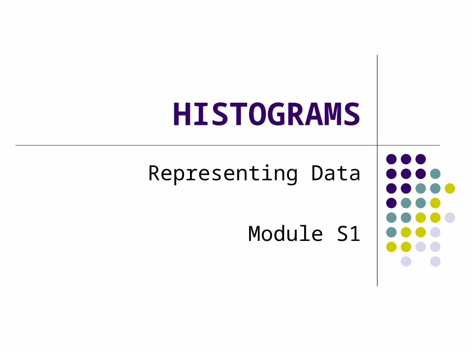
Why use a Histogram

When there is a lot of data When data is

Continuous a mass, height, volume, time etc

Presented in a Grouped Frequency Distribution usually in groups or classes that are UNEQUAL

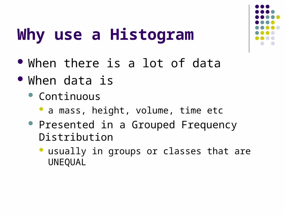
Continuous data

NO GAPS between Bars

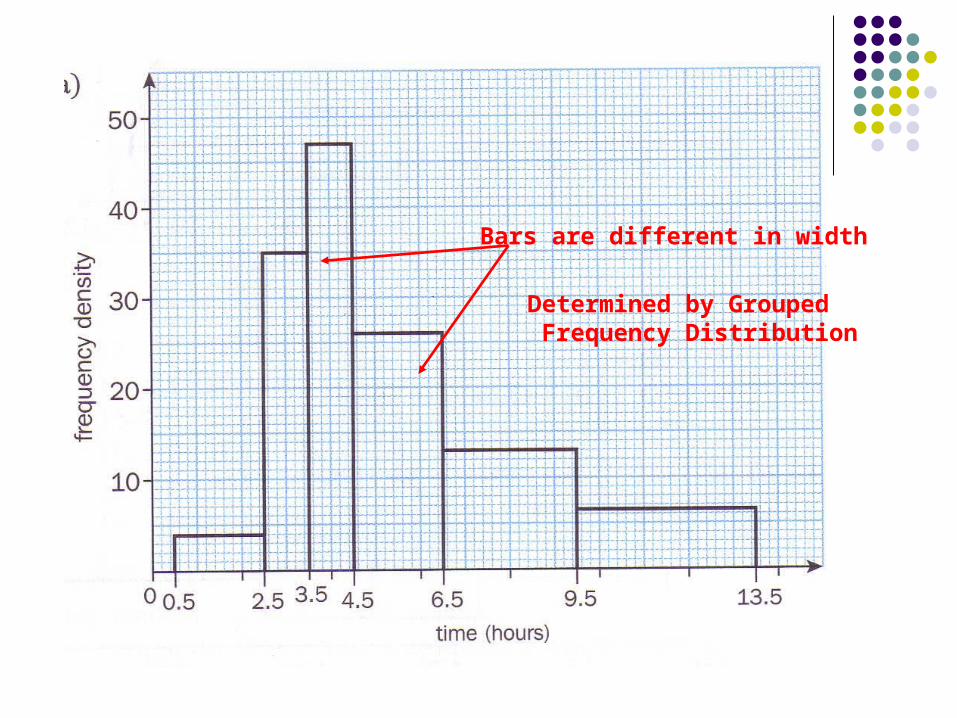
Bars are different in width

Determined by Grouped Frequency Distribution

AREA is proportional to FREQUENCY

NOT height, because of UNEQUAL classes!

So we use FREQUENCY DENSITY = Frequency Class width

Grouped Frequency Distribution

Time taken (nearest minute)

5-9 10-19 20-29 30-39 40-59

Freq 14 9 18 3 5

Speed, kph 0< v ≤40 40< v ≤50 50< v ≤60 60< v ≤90 90< v ≤110

Frequency 80 15 25 90 30

ClassesNo gaps

GAPS! Need to adjust to Continuous

Ready to graph

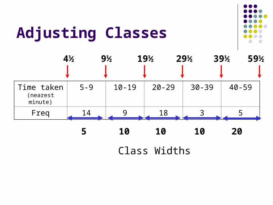
Adjusting Classes

Class Widths

Time taken (nearest minute)

5-9 10-19 20-29 30-39 40-59

Freq 14 9 18 3 5

9½4½ 19½ 29½ 39½ 59½

105 10 10 20

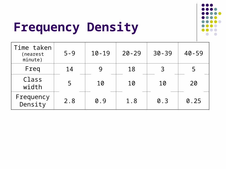
Frequency Density

Time taken (nearest minute) 5-9 10-19 20-29 30-39 40-59

Freq 14 9 18 3 5

Class width 5 10 10 10 20

Frequency Density 2.8 0.9 1.8 0.3 0.25

Drawing

Sensible Scales Bases correctly aligned

Plot the Class Boundaries Heights correct

Frequency Density

4.5 19.59.5 29.5 39.5 49.5 59.5

3.0

2.0

1.0

Fre

q D

en

s

Time (Mins)

Estimating a Frequency

Imagine we want to Estimate the number of people with a time between 12 and 25 mins

Because rounded to nearest minute Consider the interval 11.5 to 25.5

4.5 19.59.5 29.5 39.5 49.5 59.5

3.0

2.0

1.0

Fre

q D

en

s

Time (Mins)

11.5 25.5

Frequency = 0.9 x 8 = 7.2

Frequency = 1.8 x 6 = 10.8

Total Frequency = 18

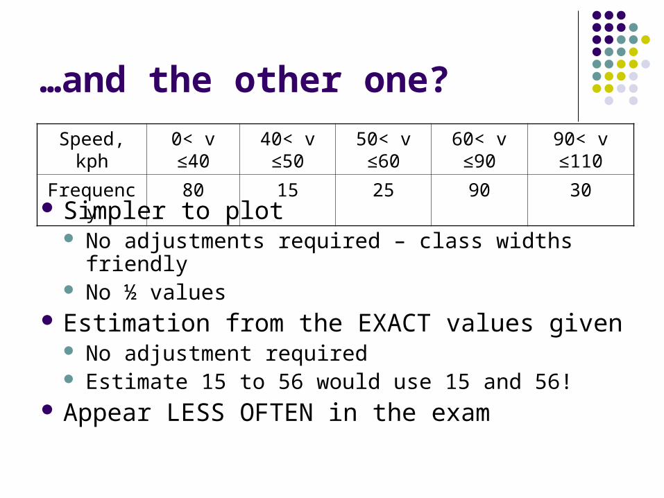
…and the other one?

Simpler to plot No adjustments required – class widths friendly No ½ values

Estimation from the EXACT values given No adjustment required Estimate 15 to 56 would use 15 and 56!

Appear LESS OFTEN in the exam

Speed, kph 0< v ≤40 40< v ≤50 50< v ≤60 60< v ≤90 90< v ≤110

Frequency 80 15 25 90 30