Hilton • Maher • Selto

Hilton Maher Selto. 12 Financial and Cost-Volume-Profit Models McGraw-Hill/Irwin © 2003 The McGraw-Hill Companies, Inc., All Rights Reserved.
Dec 21, 2015
Welcome message from author
This document is posted to help you gain knowledge. Please leave a comment to let me know what you think about it! Share it to your friends and learn new things together.
Transcript

Hilton • Maher • Selto

12Financial and Cost-Volume-Profit
Models
McGraw-Hill/Irwin © 2003 The McGraw-Hill Companies, Inc., All Rights Reserved.

12-3
Definition of Financial Models
Accurate, reliable Accurate, reliable simulations of simulations of
relations among relations among relevant costs, relevant costs,
benefits, value and benefits, value and risk that is useful for risk that is useful for supporting business supporting business
decisions.decisions.
Accurate, reliable Accurate, reliable simulations of simulations of
relations among relations among relevant costs, relevant costs,
benefits, value and benefits, value and risk that is useful for risk that is useful for supporting business supporting business
decisions.decisions.
Relationships between costs,
revenues, & income.
Relationships between costs,
revenues, & income.
Relationships between current
investments and value.
Relationships between current
investments and value.
Pro forma financial
statements.
Pro forma financial
statements.

12-4
Objectives of Financial Modeling

12-5
Basic Cost-Volume-Profit (CVP) Model
Profit = Revenue - Variable Cost - Fixed CostProfit = Revenue - Variable Cost - Fixed Cost
Makes the following assumptionsMakes the following assumptions::•Revenue can be estimated as:Revenue can be estimated as:Sales Price (SP) × Units SoldSales Price (SP) × Units Sold
•Variable Cost can be estimated as:Variable Cost can be estimated as:Variable Cost per unit (VC) × Units SoldVariable Cost per unit (VC) × Units Sold
•Fixed Cost (FC) will remain fixed over the relevant Fixed Cost (FC) will remain fixed over the relevant range.range.

12-6
CVP Model and the Break-Even Point
Profit = Revenue - Variable Cost - Fixed CostProfit = Revenue - Variable Cost - Fixed Cost
Use the above model, but assume that Profit = $0Use the above model, but assume that Profit = $0so that Break-Even is where:so that Break-Even is where:
Revenue = Variable Cost + Fixed CostRevenue = Variable Cost + Fixed Cost(SP × Sales Units) = (VC × Sales Units) + FC(SP × Sales Units) = (VC × Sales Units) + FC
Using the above relationship, we can identify the Using the above relationship, we can identify the number of units we need to sell in order to break number of units we need to sell in order to break
even.even.

12-7
Break-Even Model - Example
Planet, Inc. sells Model XT telescopes for $2,000 each. Fixed costs totaled $300,000,
variable costs were $800 per unit.How many units does Planet need to sell in
order to Break-Even?
Planet, Inc. sells Model XT telescopes for $2,000 each. Fixed costs totaled $300,000,
variable costs were $800 per unit.How many units does Planet need to sell in
order to Break-Even?
(SP × Sales Units) = (VC × Sales Units) + FC(SP × Sales Units) = (VC × Sales Units) + FC
??(SP × Sales Units) = (VC × Sales Units) + FC(SP × Sales Units) = (VC × Sales Units) + FC
??

12-8
Break-Even Model - Example
Planet, Inc. sells Model XT telescopes for $2,000 each. Fixed costs totaled $300,000,
variable costs were $800 per unit. How many units does Planet need to sell in
order to Break-Even?
Planet, Inc. sells Model XT telescopes for $2,000 each. Fixed costs totaled $300,000,
variable costs were $800 per unit. How many units does Planet need to sell in
order to Break-Even?
(SP × Sales Units) = (VC × Sales Units) + FC(SP × Sales Units) = (VC × Sales Units) + FCBreak Even Sales Units = FC ÷ (SP - VC)Break Even Sales Units = FC ÷ (SP - VC)
= $300,000 ÷ ($2,000 - $800)= $300,000 ÷ ($2,000 - $800)= $300,000 ÷ $1,200= $300,000 ÷ $1,200
= 250 Telescopes= 250 Telescopes
(SP × Sales Units) = (VC × Sales Units) + FC(SP × Sales Units) = (VC × Sales Units) + FCBreak Even Sales Units = FC ÷ (SP - VC)Break Even Sales Units = FC ÷ (SP - VC)
= $300,000 ÷ ($2,000 - $800)= $300,000 ÷ ($2,000 - $800)= $300,000 ÷ $1,200= $300,000 ÷ $1,200
= 250 Telescopes= 250 Telescopes

12-9
(SP - VC)(SP - VC)
is referred to as is referred to as Contribution Margin (CM)Contribution Margin (CM)
(SP - VC)(SP - VC)
is referred to as is referred to as Contribution Margin (CM)Contribution Margin (CM)
Contribution Margin Approach
In the previous In the previous example, we used:example, we used:
FC ÷ (SP - VC)FC ÷ (SP - VC)
to compute Break-to compute Break-Even Units.Even Units.
In the previous In the previous example, we used:example, we used:
FC ÷ (SP - VC)FC ÷ (SP - VC)
to compute Break-to compute Break-Even Units.Even Units.

12-10
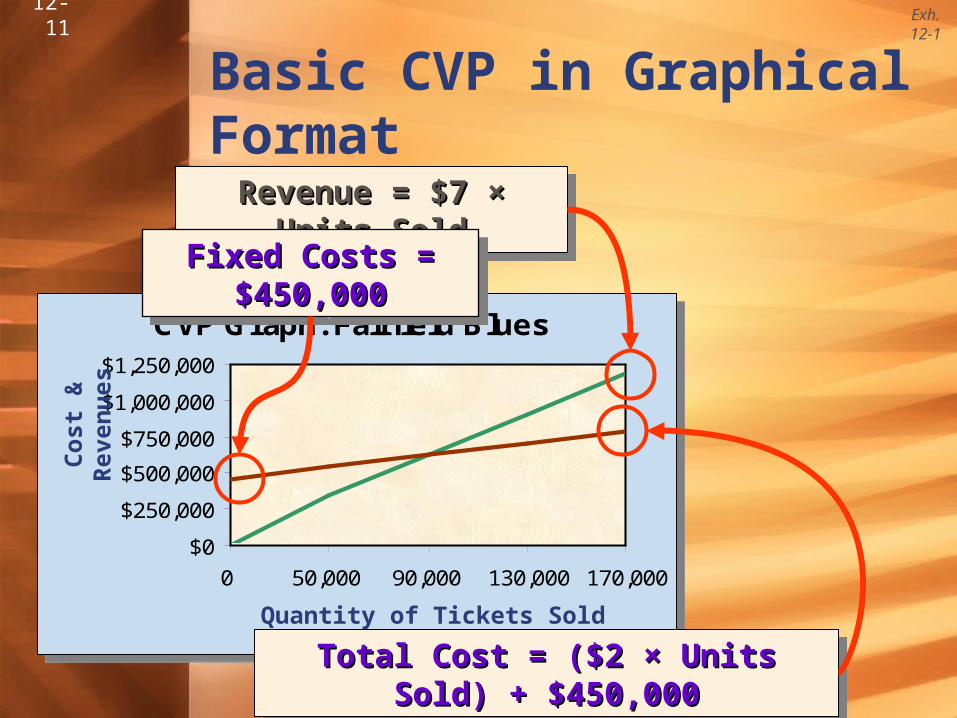
Basic CVP in Graphical Format
CVP Graph: Fairfield Blues
$0
$250,000
$500,000
$750,000
$1,000,000
$1,250,000
0 50,000 90,000 130,000 170,000
Quantity of Tickets Sold
Cos
t &
Rev
enu
es Fairfield Blues Fairfield Blues sells tickets for sells tickets for
$7. Fixed $7. Fixed Costs are Costs are
$450,000 and $450,000 and Variable Costs Variable Costs per unit are $2 per unit are $2
per ticket. per ticket.
The Revenue and Cost lines can be overlaid to get a picture The Revenue and Cost lines can be overlaid to get a picture of the CVP relationship.of the CVP relationship.
The Revenue and Cost lines can be overlaid to get a picture The Revenue and Cost lines can be overlaid to get a picture of the CVP relationship.of the CVP relationship.
Exh.12-1
12-11
CVP Graph: Fairfield Blues
$0
$250,000
$500,000
$750,000
$1,000,000
$1,250,000
0 50,000 90,000 130,000 170,000
Quantity of Tickets Sold
Cos
t &
Rev
enu
esBasic CVP in Graphical FormatRevenue = $7 × Units SoldRevenue = $7 × Units SoldRevenue = $7 × Units SoldRevenue = $7 × Units Sold
Total Cost = ($2 × Units Sold) + $450,000Total Cost = ($2 × Units Sold) + $450,000Total Cost = ($2 × Units Sold) + $450,000Total Cost = ($2 × Units Sold) + $450,000
Fixed Costs = $450,000Fixed Costs = $450,000Fixed Costs = $450,000Fixed Costs = $450,000
Exh.12-1

12-12
CVP Graph: Fairfield Blues
$0
$250,000
$500,000
$750,000
$1,000,000
$1,250,000
0 50,000 90,000 130,000 170,000
Quantity of Tickets Sold
Cos
t &
Rev
enu
esBasic CVP in Graphical Format
Profit Area is Profit Area is the amount by the amount by which revenue which revenue exceeds total exceeds total
cost.cost.
Profit Area is Profit Area is the amount by the amount by which revenue which revenue exceeds total exceeds total
cost.cost.
Loss Area is the amount by which Loss Area is the amount by which total cost exceeds revenue.total cost exceeds revenue.
Loss Area is the amount by which Loss Area is the amount by which total cost exceeds revenue.total cost exceeds revenue. Break-Even is Break-Even is
where the two where the two lines intersect.lines intersect.
Break-Even is Break-Even is where the two where the two lines intersect.lines intersect.
Exh.12-1

12-13
CVP and Target Income
Break-Even analysis uses $0 for profit. Target Profit Break-Even analysis uses $0 for profit. Target Profit analysis, puts a $ target in the profit variable, but uses the analysis, puts a $ target in the profit variable, but uses the
same model as Break-Even analysis.same model as Break-Even analysis.
Planet, Inc. sells Model XT telescopes for $2,000 each. Fixed costs are $300,000, variable costs are $800 per
unit.How many units does Planet need to sell in order to
have target profit of $120,000?
Planet, Inc. sells Model XT telescopes for $2,000 each. Fixed costs are $300,000, variable costs are $800 per
unit.How many units does Planet need to sell in order to
have target profit of $120,000?
Target Target = (SP - VC) × Sales Units - FC = (SP - VC) × Sales Units - FC
??Target Target = (SP - VC) × Sales Units - FC = (SP - VC) × Sales Units - FC
??Target Target = (SP - VC) × Sales Units - FC = (SP - VC) × Sales Units - FC
Sales Units = (Target Sales Units = (Target + FC) ÷ CM per unit + FC) ÷ CM per unit= ($120,000 + $300,000) ÷ $1,200= ($120,000 + $300,000) ÷ $1,200
= 350 Telescopes= 350 Telescopes
Target Target = (SP - VC) × Sales Units - FC = (SP - VC) × Sales Units - FCSales Units = (Target Sales Units = (Target + FC) ÷ CM per unit + FC) ÷ CM per unit
= ($120,000 + $300,000) ÷ $1,200= ($120,000 + $300,000) ÷ $1,200= 350 Telescopes= 350 Telescopes

12-14
Operating Leverage
Reflects the risk of missing sales targets.Reflects the risk of missing sales targets.
Measured as the ratio between contribution Measured as the ratio between contribution margin and operating income.margin and operating income.
Reflects the risk of missing sales targets.Reflects the risk of missing sales targets.
Measured as the ratio between contribution Measured as the ratio between contribution margin and operating income.margin and operating income.
A high operating leverage is indicative
of high committed costs (e.g. interest).
A relatively small change in sales can
lead to a loss.
A high operating leverage is indicative
of high committed costs (e.g. interest).
A relatively small change in sales can
lead to a loss.
A low operating leverage is indicative
of low committed costs (e.g. interest). More of the costs are
variable in nature.
A low operating leverage is indicative
of low committed costs (e.g. interest). More of the costs are
variable in nature.

12-15
Computer Spreadsheet Models
1. Gather all the facts,
assumptions, and estimates
for your model; i.e., parameters.
1. Gather all the facts,
assumptions, and estimates
for your model; i.e., parameters. 2. Describe the relations
between the parameters. This usually results in an
algebraic equation.
2. Describe the relations between the parameters. This usually results in an
algebraic equation.
3. Separate parameters and
formulas.
3. Separate parameters and
formulas.

12-16
Modeling Taxes
After-tax After-tax = Before-tax = Before-tax × (1 - Tax Rate) × (1 - Tax Rate)
Adding the tax rate to your profit model, will have no Adding the tax rate to your profit model, will have no effect on the computation of break-even.effect on the computation of break-even.
Adding the tax rate to your profit model will increase Adding the tax rate to your profit model will increase the number of sales units necessary to reach target the number of sales units necessary to reach target
profit.profit.
With careful planning, many investments and transactions can be structured to minimize the tax implications.
With careful planning, many investments and transactions can be structured to minimize the tax implications.

12-17
Modeling Multiple Products
When a company sells When a company sells multiple products, multiple products, modeling requires:modeling requires:
1. An estimate of the 1. An estimate of the relative proportion of relative proportion of
each product in the “each product in the “sales sales mixmix”. ”.
2. A computation of the 2. A computation of the Weighted Average Unit Weighted Average Unit
CM.CM.

12-18
Modeling Multiple Products
Planet plans to add two new telescopes to its line, The Earth II Model and the Junior Model. Relative sales and cost estimates are:
Planet plans to add two new telescopes to its line, The Earth II Model and the Junior Model. Relative sales and cost estimates are:
(CM(CM11 × Sales % × Sales %11) + (CM) + (CM22 × Sales % × Sales %22) + (CM) + (CM33 × Sales % × Sales %33))
??(CM(CM11 × Sales % × Sales %11) + (CM) + (CM22 × Sales % × Sales %22) + (CM) + (CM33 × Sales % × Sales %33))
??(CM(CM11 × Sales % × Sales %11) + (CM) + (CM22 × Sales % × Sales %22) + (CM) + (CM33 × Sales % × Sales %33))
= ($1,200 × 25%) + ($700 × 40%) + ($350 × 35%)= ($1,200 × 25%) + ($700 × 40%) + ($350 × 35%)= $300.00 + $280.00 + $122.50= $300.00 + $280.00 + $122.50
= $702.50= $702.50
(CM(CM11 × Sales % × Sales %11) + (CM) + (CM22 × Sales % × Sales %22) + (CM) + (CM33 × Sales % × Sales %33))
= ($1,200 × 25%) + ($700 × 40%) + ($350 × 35%)= ($1,200 × 25%) + ($700 × 40%) + ($350 × 35%)= $300.00 + $280.00 + $122.50= $300.00 + $280.00 + $122.50
= $702.50= $702.50

12-19
Limitations of Modeling

12-20
Modeling Multiple Cost Drivers
Cost drivers should be Cost drivers should be grouped based on their type. grouped based on their type. The cost model for multiple The cost model for multiple cost drivers would look like:cost drivers would look like:
Total Cost = (Unit variable cost × Sales Total Cost = (Unit variable cost × Sales units) + (Batch cost × Batch activity) + units) + (Batch cost × Batch activity) +
(Product cost × Product activity) + (Product cost × Product activity) + (Customer cost × Customer activity) + (Customer cost × Customer activity) +
(Facility cost × Facility activity)(Facility cost × Facility activity)
Note that Note that units sold is units sold is
no longer the no longer the sole cost sole cost driver.driver.

12-21
Theory of Constraints
5. Increase the bottleneck’s capacity
5. Increase the bottleneck’s capacity
1. Identify the appropriate
measures of value
1. Identify the appropriate
measures of value
4. Synchronize all other processes to
the bottlenecks
4. Synchronize all other processes to
the bottlenecks
6. Avoid inertia and return to Step #1
6. Avoid inertia and return to Step #1
2. Identify the bottlenecks
2. Identify the bottlenecks
3. Use bottlenecks properly
3. Use bottlenecks properly

12-22
End of Chapter 12
Yep! I’m Yep! I’m feeling feeling
constrained constrained NOW!NOW!
Related Documents