Hillslope scale soil moisture variability in a steep alpine terrain

Page 1

Journal of Hydrology 364 (2009) 311–327

Contents lists available at ScienceDirect

Journal of Hydrology

journal homepage: www.elsevier .com/locate / jhydrol

Hillslope scale soil moisture variability in a steep alpine terrain

Daniele Penna *, Marco Borga, Daniele Norbiato, Giancarlo Dalla FontanaDepartment of Land and Agroforest Environments, University of Padova, Agripolis, viale dell’Università, 16, Legnaro IT-35020, Italy

a r t i c l e i n f o

Article history:Received 11 April 2008Received in revised form 19 September2008Accepted 8 November 2008

Keywords:Soil moistureHillslope hydrologyScalingAlpine region

0022-1694/$ - see front matter � 2008 Elsevier B.V. Adoi:10.1016/j.jhydrol.2008.11.009

* Corresponding author. Tel.: +39 049 8272700; faxE-mail address: [email protected] (D. Penna)

s u m m a r y

In this study we analyse space–time variability of soil moisture data collected at 0–6, 0–12 and 0–20 cmdepth over three hillslopes with contrasting steep relief and shallow soil depth in the Dolomites (central-eastern Italian Alps). The data have been collected during two summer seasons (2005 and 2006) with dif-ferent precipitation distribution. Analysis of soil moisture data shows that different physical processescontrol the space–time distribution of soil moisture at the three soil depths, with a marked effect ofdew on the 0–6 cm soil depth layer. The range of skewness values decreases markedly from the surfaceto deeper layers. More symmetric distributions, characterised by relatively low skewness, are found formid-range soil moisture contents, while highly skewed distributions (generally with more log–normalshape) are found at dry and wet conditions. Scatter plots drawn for the whole data set and the analysisof the correlation coefficients suggest a good persistence of soil moisture with depth: the highest degreeof correlation was observed between data collected at 0–12 and 0–20 cm.

Examination of correlation between soil moisture fields and topographical attributes shows that, not-withstanding the steep relief and the humid conditions, terrain indices are relatively poor predictors ofsoil moisture spatial variability. The slope and the topographic wetness index, which are found herethe best univariate spatial predictors of soil moisture, explains up to 42% of the time-averaged moisturespatial variation.

A negative relationship between the soil moisture spatial mean and the corresponding spatial standarddeviation is found for mean water contents exceeding 25–30%, while a transition to a positive relation-ship is observed with drier conditions. Overall, soil moisture variability shows the highest values at mod-erate moisture conditions (23–29%) and reduced values for wetter and drier conditions for all depths. Anegative linear relationship between mean soil moisture content and the coefficient of variation wasobserved.

A soil moisture dynamics model proved to successfully capture the soil moisture variability at the hill-slope scale. The simulated time series of hillslope-averaged soil moisture are in good agreement with theobserved ones. Moreover, the model reproduces consistently the observed relationships between soilmoisture spatial mean and corresponding variability.

� 2008 Elsevier B.V. All rights reserved.

Introduction

Soil moisture plays a central role in the global water cycle bycontrolling the partitioning of water and energy fluxes at theearth’s surface and constitutes the physical linkage between soil,climate and vegetation (Albertson and Montaldo, 2003; Pan et al.,2003; Rodríguez-Iturbe and Porporato, 2004). At the point scalesoil moisture is crucial for the infiltration process (Bronstert andBárdossy, 1999; Raats, 2001) and plant dynamics (Porporatoet al., 2004). At the hillslope and catchment scale, the spatial andtemporal distribution of soil moisture controls the flood formationprocess (Borga et al., 2007). At the regional and continental scale,

ll rights reserved.

: +39 049 8272686..

soil moisture controls water distribution through land surfaceatmosphere feedback mechanisms (Koster et al., 2004).

Due to soil heterogeneity, atmospheric forcing, vegetation andtopography, soil moisture is variable in space and time. Under-standing and characterizing this variability is one of the majorchallenges within hydrological sciences. Information characteriz-ing space–time variability of soil moisture is important to under-stand the contribution of soil moisture variability at smallerscales towards the effective soil moisture observed at larger scalesor its role in the parametrization of, e.g., climate and watershedmodels (Famiglietti et al., 1999; Ryu and Famiglietti, 2005). Assuch, this information can provide guidelines for the design of fieldexperiments and for the efficient use of remote sensing estimates.

Characterization of space–time soil moisture variability hasbeen attempted by analysing the trends of spatial soil moisture

Page 2

312 D. Penna et al. / Journal of Hydrology 364 (2009) 311–327

variability with spatial mean moisture content. Empirical analysesfound that, generally, the standard deviation increases during dry-ing from a very wet stage, reaches a maximum value at a specific orcritical mean moisture content and then decreases during furtherdrying (Famiglietti et al., 2008). Western et al. (2003) provided aqualitative interpretation of why variance peaks at intermediatemoisture contents by making use of the combined results fromseveral field campaigns. In their interpretation, differences inbehaviour in humid and semiarid regions are related to differencesin the patterns of controlling processes. They found that the loca-tion and magnitude of the variance peak changed between catch-ments. Depth appeared to have only a small effect on therelationship. In the last 10 years, a number of studies have at-tempted to examine quantitatively how different processes act toeither increase or decrease the spatial variability of soil moisture.By using the similar media concept, Salvucci (1998) showed howvariability in soil texture leads to different soil moisture variabilitystates in different limiting cases. Albertson and Montaldo (2003)showed how covariances between soil moisture and fluxes, origi-nating from variability in soil moisture, forcing and/or land surfaceproperties, can lead to either an increase or decrease in soil mois-ture variability. Teuling et al. (2005) developed a simple soil mois-ture dynamics model and showed how vegetation, soil andtopography controls interact to either create or destroy spatialvariance. By accounting for effects of spatial variability in soiland vegetation characteristics, in combination with atmosphericforcing (precipitation and potential evapotranspiration), differentobserved relations between spatial mean soil moisture and its var-iability can be explained in this way. Using stochastic analysis ofthe unsaturated Brooks–Corey flow in heterogeneous soils, Vereec-ken et al. (2007) showed that parameters of the moisture retentioncharacteristic and their spatial variability determine to a large ex-tent the shape of the soil moisture variance–mean water contentrelationship. They found that the standard deviation of soil mois-ture peaked between 0.17% and 0.23% for most textural classesand that the peak value was controlled by the parameters whichdescribe the pore size distribution of soils. The theoretical resultsobtained by Vereecken et al. (2007) correspond well with Ryuand Famiglietti (2005) who experimentally found that the soilmoisture variance–mean water content relationship tends to peakaround a value of 0.2%.

These studies generally examined soil moisture variability forgentle topographies. Examples are provided by the Tarrawarraand Mahurangi experiments (Western and Grayson, 1998, 2000,

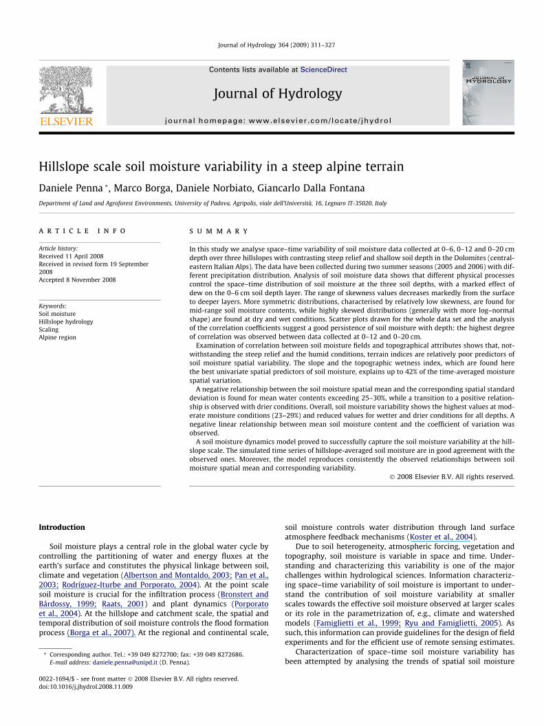
Figure 1. Rio Vauz catchment and

1999, 2004; Wilson et al., 2003, 2004) and SGP97, SGP99, SMEX02and SMEX03 (Famiglietti et al., 1999; Mohanty and Skaggs, 2001;Choi and Jacobs, 2007). Few field studies have examined variabilityof soil moisture patterns in steep terrain and high altitude (abovetree line) conditions (Grant et al., 2004). In general, the spatial var-iability of soil moisture in mountainous regions is expected to behigh relative to other landscapes due to heterogeneous conditionsof surface and bedrock topography, soil characteristics, wind pat-terns, interaction between evaporation, condensation and precipi-tation. Moreover, it is expected that the soil moisture spatialvariability in humid and steep conditions with shallow soils (morefavourable to lateral flow occurrence) exhibits a stronger relation-ship with topographic variables than in more gently sloping land-scape (Grayson and Western, 2001).

The main objective of this study is to characterise the variabilityof field scale soil moisture for three hillslopes characterised by con-trasting steep relief and shallow soil depth located in the highmountainous Vauz river basin (Dolomites, central eastern ItalianAlps). Soil moisture data were collected over three depths: 0–6,0–12 and 0–20 cm. The three hillslopes show marked differencesin topography, representing concave, planar and convex structure.Because of the relative small area, we do not expect significant dif-ferences in precipitation, relative air humidity, temperature andother climatic variables. This allows to isolate the effects of topog-raphy and soil depths on space–time variability of soil moisturefields. The hillslopes considered may be deemed representativeof pedological, topographic, climatic conditions frequently met inpasture areas of the Dolomites.

Based on these data, this study (1) characterises the statisticalproperties of the soil moisture measurements with varying soildepth and hillslope topography, and investigates the correlationbetween soil moisture measurements collected at various soildepths; (2) examines the influence of topographic variables on soilmoisture spatial variability; (3) investigates the relationship be-tween mean moisture content and spatial variability and (4) anal-yses the suitability of applying a soil moisture variability dynamicsmodel to reproduce the observed spatial mean moisture content –spatial variability relationship. The use of a water balance model tocharacterise the spatial and temporal organization of soil moisturefields is appealing, since this could reduce the need for groundbased measurements significantly in numerous applications. Themodel applied here (Teuling and Troch, 2005) accounts for varia-tions in soil and vegetation properties but not for redistributiondue to lateral flow. It is therefore interesting to evaluate the quality

location of the three hillslopes.

Page 3

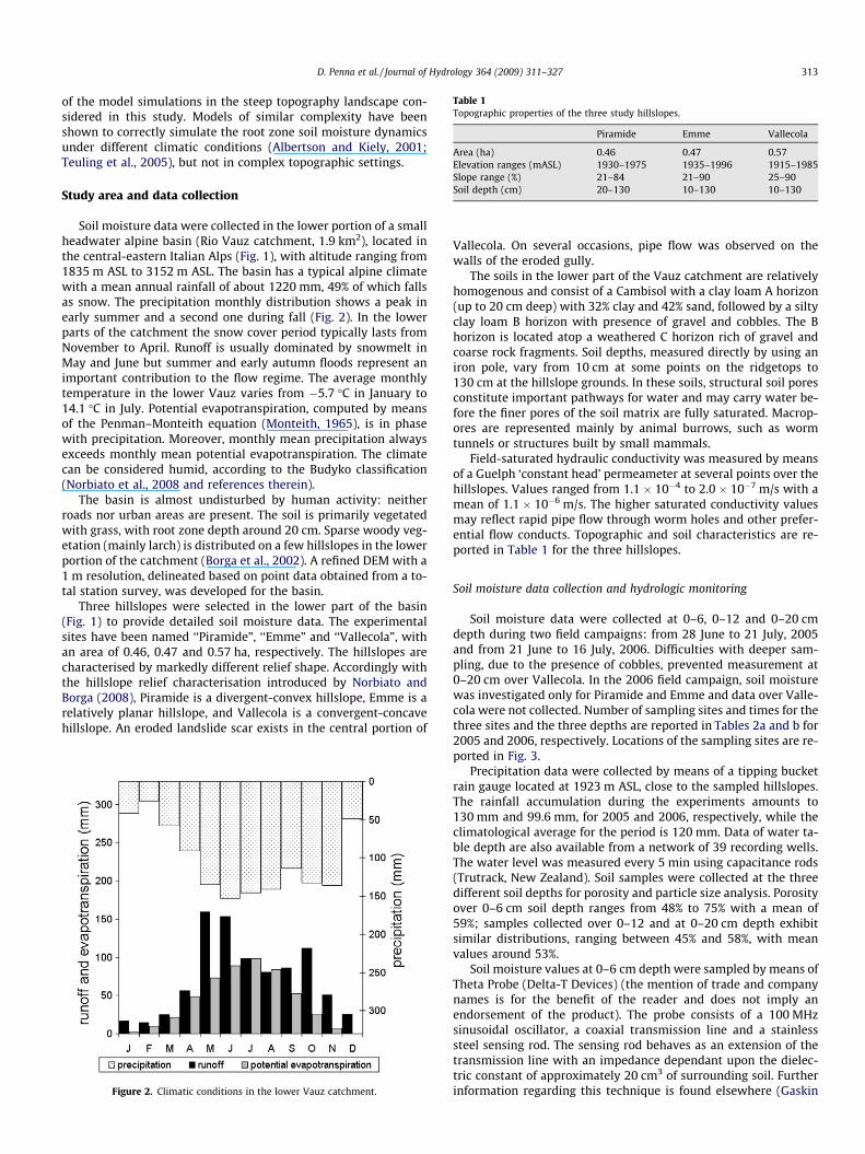
Table 1Topographic properties of the three study hillslopes.

Piramide Emme Vallecola

Area (ha) 0.46 0.47 0.57Elevation ranges (mASL) 1930–1975 1935–1996 1915–1985Slope range (%) 21–84 21–90 25–90Soil depth (cm) 20–130 10–130 10–130

D. Penna et al. / Journal of Hydrology 364 (2009) 311–327 313

of the model simulations in the steep topography landscape con-sidered in this study. Models of similar complexity have beenshown to correctly simulate the root zone soil moisture dynamicsunder different climatic conditions (Albertson and Kiely, 2001;Teuling et al., 2005), but not in complex topographic settings.

Study area and data collection

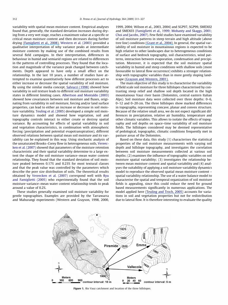
Soil moisture data were collected in the lower portion of a smallheadwater alpine basin (Rio Vauz catchment, 1.9 km2), located inthe central-eastern Italian Alps (Fig. 1), with altitude ranging from1835 m ASL to 3152 m ASL. The basin has a typical alpine climatewith a mean annual rainfall of about 1220 mm, 49% of which fallsas snow. The precipitation monthly distribution shows a peak inearly summer and a second one during fall (Fig. 2). In the lowerparts of the catchment the snow cover period typically lasts fromNovember to April. Runoff is usually dominated by snowmelt inMay and June but summer and early autumn floods represent animportant contribution to the flow regime. The average monthlytemperature in the lower Vauz varies from �5.7 �C in January to14.1 �C in July. Potential evapotranspiration, computed by meansof the Penman–Monteith equation (Monteith, 1965), is in phasewith precipitation. Moreover, monthly mean precipitation alwaysexceeds monthly mean potential evapotranspiration. The climatecan be considered humid, according to the Budyko classification(Norbiato et al., 2008 and references therein).

The basin is almost undisturbed by human activity: neitherroads nor urban areas are present. The soil is primarily vegetatedwith grass, with root zone depth around 20 cm. Sparse woody veg-etation (mainly larch) is distributed on a few hillslopes in the lowerportion of the catchment (Borga et al., 2002). A refined DEM with a1 m resolution, delineated based on point data obtained from a to-tal station survey, was developed for the basin.

Three hillslopes were selected in the lower part of the basin(Fig. 1) to provide detailed soil moisture data. The experimentalsites have been named ‘‘Piramide”, ‘‘Emme” and ‘‘Vallecola”, withan area of 0.46, 0.47 and 0.57 ha, respectively. The hillslopes arecharacterised by markedly different relief shape. Accordingly withthe hillslope relief characterisation introduced by Norbiato andBorga (2008), Piramide is a divergent-convex hillslope, Emme is arelatively planar hillslope, and Vallecola is a convergent-concavehillslope. An eroded landslide scar exists in the central portion of

Figure 2. Climatic conditions in the lower Vauz catchment.

Vallecola. On several occasions, pipe flow was observed on thewalls of the eroded gully.

The soils in the lower part of the Vauz catchment are relativelyhomogenous and consist of a Cambisol with a clay loam A horizon(up to 20 cm deep) with 32% clay and 42% sand, followed by a siltyclay loam B horizon with presence of gravel and cobbles. The Bhorizon is located atop a weathered C horizon rich of gravel andcoarse rock fragments. Soil depths, measured directly by using aniron pole, vary from 10 cm at some points on the ridgetops to130 cm at the hillslope grounds. In these soils, structural soil poresconstitute important pathways for water and may carry water be-fore the finer pores of the soil matrix are fully saturated. Macrop-ores are represented mainly by animal burrows, such as wormtunnels or structures built by small mammals.

Field-saturated hydraulic conductivity was measured by meansof a Guelph ‘constant head’ permeameter at several points over thehillslopes. Values ranged from 1.1 � 10�4 to 2.0 � 10�7 m/s with amean of 1.1 � 10�6 m/s. The higher saturated conductivity valuesmay reflect rapid pipe flow through worm holes and other prefer-ential flow conducts. Topographic and soil characteristics are re-ported in Table 1 for the three hillslopes.

Soil moisture data collection and hydrologic monitoring

Soil moisture data were collected at 0–6, 0–12 and 0–20 cmdepth during two field campaigns: from 28 June to 21 July, 2005and from 21 June to 16 July, 2006. Difficulties with deeper sam-pling, due to the presence of cobbles, prevented measurement at0–20 cm over Vallecola. In the 2006 field campaign, soil moisturewas investigated only for Piramide and Emme and data over Valle-cola were not collected. Number of sampling sites and times for thethree sites and the three depths are reported in Tables 2a and b for2005 and 2006, respectively. Locations of the sampling sites are re-ported in Fig. 3.

Precipitation data were collected by means of a tipping bucketrain gauge located at 1923 m ASL, close to the sampled hillslopes.The rainfall accumulation during the experiments amounts to130 mm and 99.6 mm, for 2005 and 2006, respectively, while theclimatological average for the period is 120 mm. Data of water ta-ble depth are also available from a network of 39 recording wells.The water level was measured every 5 min using capacitance rods(Trutrack, New Zealand). Soil samples were collected at the threedifferent soil depths for porosity and particle size analysis. Porosityover 0–6 cm soil depth ranges from 48% to 75% with a mean of59%; samples collected over 0–12 and at 0–20 cm depth exhibitsimilar distributions, ranging between 45% and 58%, with meanvalues around 53%.

Soil moisture values at 0–6 cm depth were sampled by means ofTheta Probe (Delta-T Devices) (the mention of trade and companynames is for the benefit of the reader and does not imply anendorsement of the product). The probe consists of a 100 MHzsinusoidal oscillator, a coaxial transmission line and a stainlesssteel sensing rod. The sensing rod behaves as an extension of thetransmission line with an impedance dependant upon the dielec-tric constant of approximately 20 cm3 of surrounding soil. Furtherinformation regarding this technique is found elsewhere (Gaskin

Page 4

Table 2aNumber of soil moisture measurements for 2005.

Piramide Emme Vallecola

0–6 cm 0–12 cm 0–20 cm 0–6 cm 0–12 cm 0–20 cm 0–6 cm 0–12 cm

No. of sampling points 26 26 26 26 26 26 16 16No. of sampling times 24 24 8 25 25 16 24 24Total no. of measures 624 624 208 650 650 416 384 384

Table 2bNumber of soil moisture measurements for 2006.

Piramide Emme Vallecola

0–6 cm 0–12 cm 0–20 cm 0–6 cm 0–12 cm 0–20 cm 0–6 cm 0–12 cm

No. of sampling points 26 26 26 26 26 26 0 0No. of sampling times 23 23 23 23 23 23 0 0Total no. of measures 598 598 598 598 598 598 0 0

314 D. Penna et al. / Journal of Hydrology 364 (2009) 311–327

and Miller, 1996; Miller et al., 1997). Soil moisture at 0–12 and 0–20 cm depth was evaluated by means of a TDR 300, a portableprobe manufactured by Spectrum Technologies Inc. (the mentionof trade and company names is for the benefit of the reader anddoes not imply an endorsement of the product) and operating onthe basis of time domain reflectometry technology. The TDR probeis provided with two pairs of interchangeable rods of 12 cm and20 cm length which allow to sample soil moisture over these dif-ferent depths.

Both Theta Probe and TDR 300 were gravimetrically calibratedfor the specific local soil conditions (Stenger et al., 2005; Walkeret al., 2004). A split tube soil sampler was used in the field to obtainundisturbed samples and 55, 45 and 40 soil cores were collected atthe three investigated depths (0–6, 0–12 and 0–20 cm), respec-tively. Sampling was carried out so that the collected cores werecharacterised by different water contents, necessary to calibrate

Figure 3. Position of sampling points ov

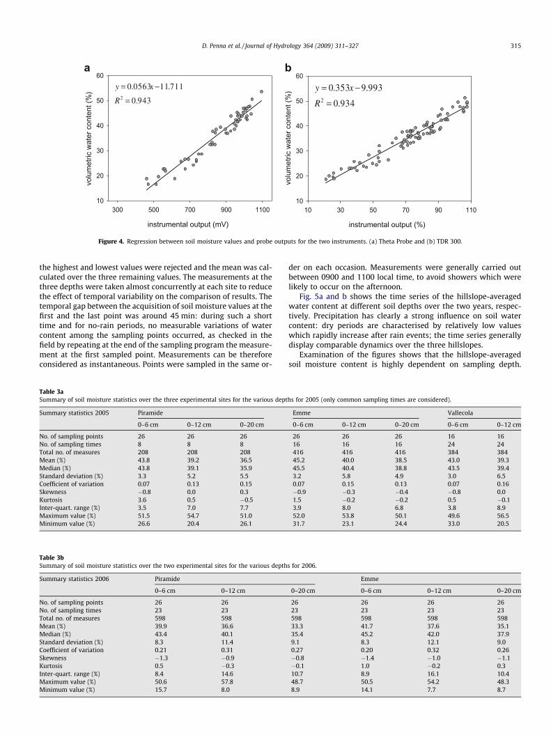
the instruments with soil conditions varying from a dry to a wetstatus (Kaleita et al., 2005). The soil samples were weighted,oven-dried at 105 �C for 24 h and weighted again and a calibrationcurve was obtained for each instrument plotting measured volu-metric versus probe-derived soil moisture values (Fig. 4). For TDR300, samples of both depths (12 and 20 cm) were used togethersince they appeared to fit the same relationship. Calibration curvesexhibit a root mean squared error (computed as in Cosh et al., 2005)of 2.35% and 2.09% for Theta Probe and TDR 300, respectively, withstandard deviations of errors equal to 2.37% for Theta Probe and2.1% for TDR 300. Bias is negligible. Note that throughout the papersoil water content is always reported as volumetric soil moisture.

Soil moisture was measured at 26 sites over Piramide andEmme, and at 16 sites over Vallecola (Tables 2 and 3; Fig. 3). Ateach measurement point, five measures were collected in orderto ascertain the repeatability of the results and instrument errors;

er the three experimental hillslopes.

Page 5

instrumental output (mV)

300 500 700 900 1100

volu

met

ric w

ater

con

tent

(%)

10

20

30

40

50

60

943.0

711.110563.02 =

−=

R

xy

instrumental output (%)

10 30 50 70 90 110

volu

met

ric w

ater

con

tent

(%)

10

20

30

40

50

60

934.0

993.9353.02 =

−=R

xy

a b

Figure 4. Regression between soil moisture values and probe outputs for the two instruments. (a) Theta Probe and (b) TDR 300.

D. Penna et al. / Journal of Hydrology 364 (2009) 311–327 315

the highest and lowest values were rejected and the mean was cal-culated over the three remaining values. The measurements at thethree depths were taken almost concurrently at each site to reducethe effect of temporal variability on the comparison of results. Thetemporal gap between the acquisition of soil moisture values at thefirst and the last point was around 45 min: during such a shorttime and for no-rain periods, no measurable variations of watercontent among the sampling points occurred, as checked in thefield by repeating at the end of the sampling program the measure-ment at the first sampled point. Measurements can be thereforeconsidered as instantaneous. Points were sampled in the same or-

Table 3aSummary of soil moisture statistics over the three experimental sites for the various dept

Summary statistics 2005 Piramide

0–6 cm 0–12 cm 0–20 cm

No. of sampling points 26 26 26No. of sampling times 8 8 8Total no. of measures 208 208 208Mean (%) 43.8 39.2 36.5Median (%) 43.8 39.1 35.9Standard deviation (%) 3.3 5.2 5.5Coefficient of variation 0.07 0.13 0.15Skewness �0.8 0.0 0.3Kurtosis 3.6 0.5 �0.5Inter-quart. range (%) 3.5 7.0 7.7Maximum value (%) 51.5 54.7 51.0Minimum value (%) 26.6 20.4 26.1

Table 3bSummary of soil moisture statistics over the two experimental sites for the various depth

Summary statistics 2006 Piramide

0–6 cm 0–12 cm

No. of sampling points 26 26No. of sampling times 23 23Total no. of measures 598 598Mean (%) 39.9 36.6Median (%) 43.4 40.1Standard deviation (%) 8.3 11.4Coefficient of variation 0.21 0.31Skewness �1.3 �0.9Kurtosis 0.5 �0.3Inter-quart. range (%) 8.4 14.6Maximum value (%) 50.6 57.8Minimum value (%) 15.7 8.0

der on each occasion. Measurements were generally carried outbetween 0900 and 1100 local time, to avoid showers which werelikely to occur on the afternoon.

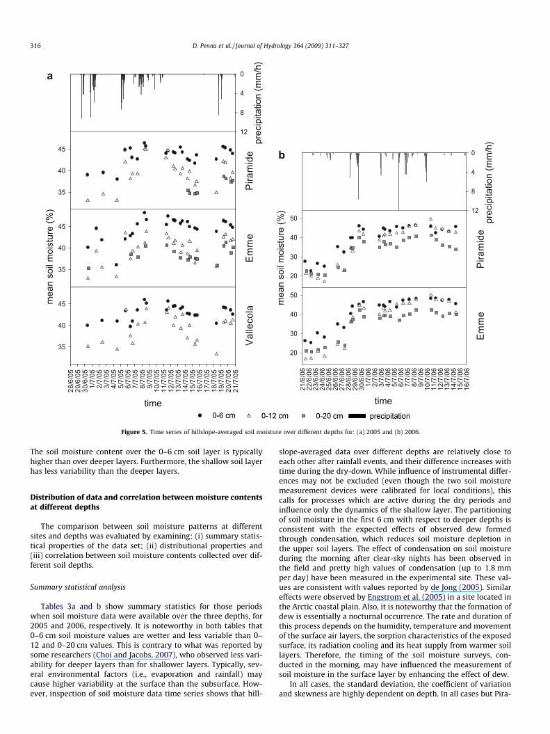
Fig. 5a and b shows the time series of the hillslope-averagedwater content at different soil depths over the two years, respec-tively. Precipitation has clearly a strong influence on soil watercontent: dry periods are characterised by relatively low valueswhich rapidly increase after rain events; the time series generallydisplay comparable dynamics over the three hillslopes.

Examination of the figures shows that the hillslope-averagedsoil moisture content is highly dependent on sampling depth.

hs for 2005 (only common sampling times are considered).

Emme Vallecola

0–6 cm 0–12 cm 0–20 cm 0–6 cm 0–12 cm

26 26 26 16 1616 16 16 24 24416 416 416 384 38445.2 40.0 38.5 43.0 39.345.5 40.4 38.8 43.5 39.43.2 5.8 4.9 3.0 6.50.07 0.15 0.13 0.07 0.16�0.9 �0.3 �0.4 �0.8 0.01.5 �0.2 �0.2 0.5 �0.13.9 8.0 6.8 3.8 8.952.0 53.8 50.1 49.6 56.531.7 23.1 24.4 33.0 20.5

s for 2006.

Emme

0–20 cm 0–6 cm 0–12 cm 0–20 cm

26 26 26 2623 23 23 23598 598 598 59833.3 41.7 37.6 35.135.4 45.2 42.0 37.99.1 8.3 12.1 9.00.27 0.20 0.32 0.26�0.8 �1.4 �1.0 �1.1�0.1 1.0 �0.2 0.310.7 8.9 16.1 10.448.7 50.5 54.2 48.38.9 14.1 7.7 8.7

Page 6

prec

ipita

tion

(mm

/h)

0

4

8

12

35

40

45

Pira

mid

e

mea

n so

il m

oist

ure

(%)

35

40

45

Emm

e

time

28/6

/05

29/6

/05

30/6

/05

1/7/

052/

7/05

3/7/

054/

7/05

5/7/

056/

7/05

7/7/

058/

7/05

9/7/

0510

/7/0

511

/7/0

512

/7/0

513

/7/0

514

/7/0

515

/7/0

516

/7/0

517

/7/0

518

/7/0

519

/7/0

520

/7/0

521

/7/0

5

35

40

45

Valle

cola

prec

ipita

tion

(mm

/h)

0

4

8

12

20

30

40

50

Pira

mid

e

time

21/6

/06

22/6

/06

23/6

/06

24/6

/06

25/6

/06

26/6

/06

27/6

/06

28/6

/06

29/6

/06

30/6

/06

1/7/

062/

7/06

3/7/

064/

7/06

5/7/

066/

7/06

7/7/

068/

7/06

9/7/

0610

/7/0

611

/7/0

612

/7/0

613

/7/0

614

/7/0

615

/7/0

616

/7/0

6

mea

n so

il m

oist

ure

(%)

20

30

40

50

Emm

e

a

b

Figure 5. Time series of hillslope-averaged soil moisture over different depths for: (a) 2005 and (b) 2006.

316 D. Penna et al. / Journal of Hydrology 364 (2009) 311–327

The soil moisture content over the 0–6 cm soil layer is typicallyhigher than over deeper layers. Furthermore, the shallow soil layerhas less variability than the deeper layers.

Distribution of data and correlation between moisture contentsat different depths

The comparison between soil moisture patterns at differentsites and depths was evaluated by examining: (i) summary statis-tical properties of the data set; (ii) distributional properties and(iii) correlation between soil moisture contents collected over dif-ferent soil depths.

Summary statistical analysis

Tables 3a and b show summary statistics for those periodswhen soil moisture data were available over the three depths, for2005 and 2006, respectively. It is noteworthy in both tables that0–6 cm soil moisture values are wetter and less variable than 0–12 and 0–20 cm values. This is contrary to what was reported bysome researchers (Choi and Jacobs, 2007), who observed less vari-ability for deeper layers than for shallower layers. Typically, sev-eral environmental factors (i.e., evaporation and rainfall) maycause higher variability at the surface than the subsurface. How-ever, inspection of soil moisture data time series shows that hill-

slope-averaged data over different depths are relatively close toeach other after rainfall events, and their difference increases withtime during the dry-down. While influence of instrumental differ-ences may not be excluded (even though the two soil moisturemeasurement devices were calibrated for local conditions), thiscalls for processes which are active during the dry periods andinfluence only the dynamics of the shallow layer. The partitioningof soil moisture in the first 6 cm with respect to deeper depths isconsistent with the expected effects of observed dew formedthrough condensation, which reduces soil moisture depletion inthe upper soil layers. The effect of condensation on soil moistureduring the morning after clear-sky nights has been observed inthe field and pretty high values of condensation (up to 1.8 mmper day) have been measured in the experimental site. These val-ues are consistent with values reported by de Jong (2005). Similareffects were observed by Engstrom et al. (2005) in a site located inthe Arctic coastal plain. Also, it is noteworthy that the formation ofdew is essentially a nocturnal occurrence. The rate and duration ofthis process depends on the humidity, temperature and movementof the surface air layers, the sorption characteristics of the exposedsurface, its radiation cooling and its heat supply from warmer soillayers. Therefore, the timing of the soil moisture surveys, con-ducted in the morning, may have influenced the measurement ofsoil moisture in the surface layer by enhancing the effect of dew.

In all cases, the standard deviation, the coefficient of variationand skewness are highly dependent on depth. In all cases but Pira-

Page 7

soil moisture (%)

0 10 20 30 40 50 60 70

frequ

ency

(%)

0

10

20

30

40

50 Piramide 0-6 cmEmme 0-6 cm

soil moisture (%)

0 10 20 30 40 50 60 70

frequ

ency

(%)

0

5

10

15

20

25

30Piramide 0-12 cmEmme 0-12 cm

soil moisture (%)

0 10 20 30 40 50 60 70

frequ

ency

(%)

0

10

20

30

40Piramide 0-20 cmEmme 0-20 cm

a b

c

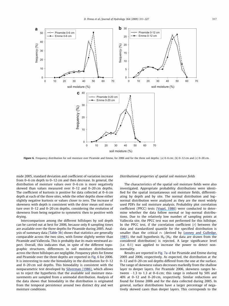
Figure 6. Frequency distribution for soil moisture over Piramide and Emme, for 2006 and for the three soil depths: (a) 0–6 cm; (b) 0–12 cm and (c) 0–20 cm.

D. Penna et al. / Journal of Hydrology 364 (2009) 311–327 317

mide 2005, standard deviation and coefficient of variation increasefrom 0–6 cm depth to 0–12 cm and then decrease. In general, thedistribution of moisture values over 0–6 cm is more negativelyskewed than values measured over 0–12 and 0–20 cm depths.The coefficient of kurtosis is positive for data collected at 0–6 cmdepth at each of the three sites, while the other depths show eitherslightly negative kurtosis or values closer to zero. The increase ofskewness with depth is consistent with the drier mean soil mois-ture over 0–12 and 0–20 cm depths, considering the evolution ofskewness from being negative to symmetric then to positive withdrying.

Intercomparison among the different hillslopes by soil depthcan be carried out at best for 2006, because only 8 sampling timesare available over the three depths for Piramide during 2005. Anal-ysis of summary data (Table 3b) shows that statistics are generallycomparable across the two sites, with Emme slightly wetter thanPiramide and Vallecola. This is probably due its main westward as-pect. Overall, this indicates that, in spite of the different topo-graphic structures, differences in soil moisture distributionsacross the three hillslopes are negligible. Frequency plots for Emmeand Piramide over the three depths are reported in Fig. 6 for 2006.It is interesting to note the bimodality in the distribution for 0–12and 0–20 cm soil depths. This bimodality is consistent with thenonparametric test developed by Silverman (1986), which allowsus to reject the hypothesis that the available soil moisture mea-surements are sampled from a unimodal distribution. Analysis ofthe data shows that bimodality in the distribution is originatedfrom the temporal persistence around two distinct dry and wetmoisture conditions.

Distributional properties of spatial soil moisture fields

The characteristics of the spatial soil moisture fields were alsoinvestigated. Appropriate probability distributions were identi-fied for the spatial instantaneous soil moisture fields, differenti-ating by depth and by site. The normal distribution and log–normal distribution were analyzed as they are the most widelyused PDFs for soil moisture analysis. Probability plot correlationcoefficient (PPCC) tests (Vogel, 1986) were conducted to deter-mine whether the data follow normal or log–normal distribu-tions. Due to the relatively low number of sampling points atVallecola site, the PPCC test was not performed for this hillslope.In the PPCC test, if the correlation coefficient (r) between thedata and standardized quantile for the specified distribution issmaller than the critical r� (derived by Looney and Gulledge,1985), the null hypothesis H0 (H0: the data are drawn from theconsidered distribution) is rejected. A large significance level(i.e. 0.1) was applied to increase the power to detect non-normality.

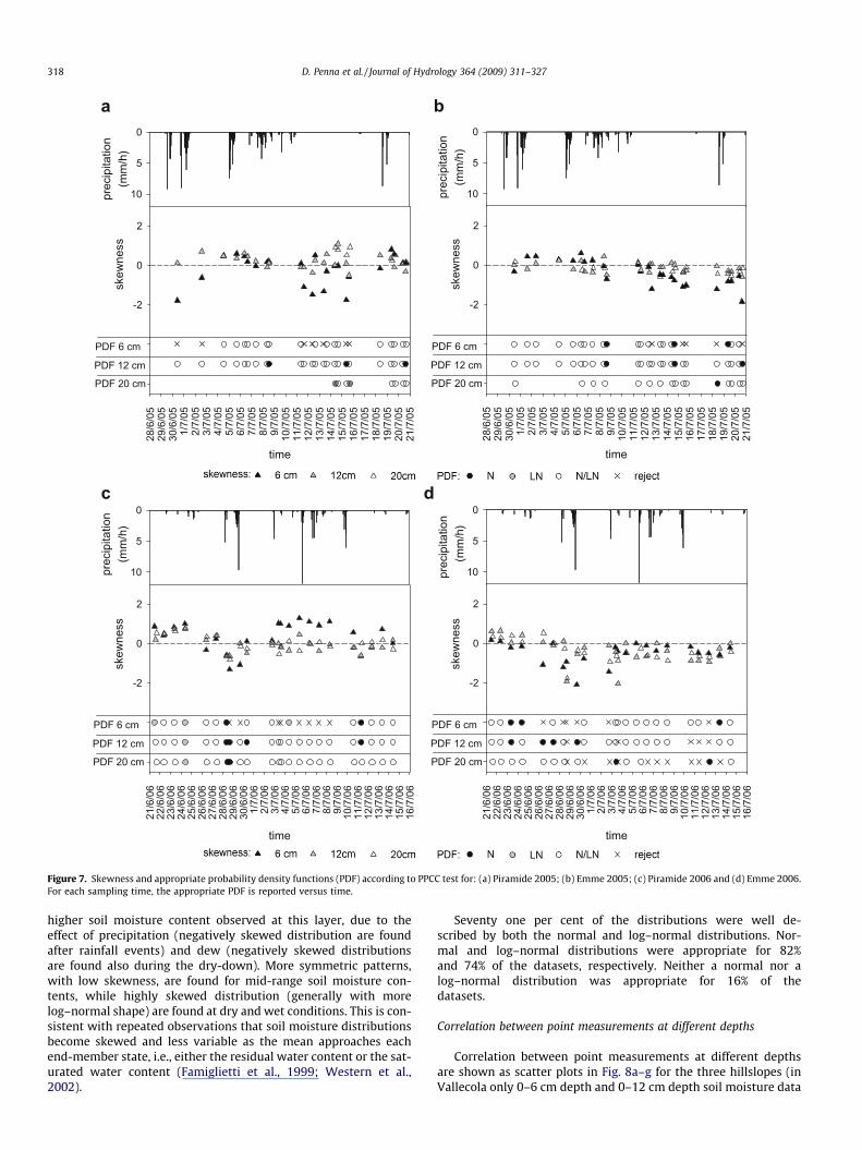
Results are reported in Fig. 7a–d for Piramide and Emme during2005 and 2006, respectively. As expected, the distribution at the0–12 and 0–20 cm soil depths differed from the one at the surface.The range of skewness values decreases markedly from the shallowlayer to deeper layers. For Piramide 2006, skewness ranges be-tween �1.3 to 1.3 at 0–6 cm; this range is reduced by 50% and40% at 0–12 and 0–20 cm, respectively. Similar reductions arefound for Emme 2006 and for the data collected during 2005. Ingeneral, surface distributions have a larger percentage of nega-tively skewed cases than deeper layers. This corresponds to the

Page 8

prec

ipita

tion

(m

m/h

)0

5

10

time

28/6

/05

29

/6/0

5

30/6

/05

1/

7/05

2/

7/05

3/

7/05

4/

7/05

5/

7/05

6/

7/05

7/

7/05

8/

7/05

9/

7/05

10

/7/0

5

11/7

/05

12

/7/0

5

13/7

/05

14

/7/0

5

15/7

/05

16

/7/0

5

17/7

/05

18

/7/0

5

19/7

/05

20

/7/0

5

21/7

/05

skew

ness

-2

0

2

PDF 6 cm

PDF 12 cm

PDF 20 cm

prec

ipita

tion

(m

m/h

)

0

5

10

time

28/6

/05

29

/6/0

5

30/6

/05

1/

7/05

2/

7/05

3/

7/05

4/

7/05

5/

7/05

6/

7/05

7/

7/05

8/

7/05

9/

7/05

10

/7/0

5

11/7

/05

12

/7/0

5

13/7

/05

14

/7/0

5

15/7

/05

16

/7/0

5

17/7

/05

18

/7/0

5

19/7

/05

20

/7/0

5

21/7

/05

skew

ness

-2

0

2

PDF 6 cm

PDF 12 cm

PDF 20 cm

prec

ipita

tion

(m

m/h

)

0

5

10

time

21/6

/06

22

/6/0

6

23/6

/06

24

/6/0

6

25/6

/06

26

/6/0

6

27/6

/06

28

/6/0

6

29/6

/06

30

/6/0

6

1/7/

06

2/7/

06

3/7/

06

4/7/

06

5/7/

06

6/7/

06

7/7/

06

8/7/

06

9/7/

06

10/7

/06

11

/7/0

6

12/7

/06

13

/7/0

6

14/7

/06

15

/7/0

6

16/7

/06

skew

ness

-2

0

2

PDF 6 cm

PDF 12 cm

PDF 20 cm

prec

ipita

tion

(mm

/h)

0

5

10

time

21/6

/06

22

/6/0

6

23/6

/06

24

/6/0

6

25/6

/06

26

/6/0

6

27/6

/06

28

/6/0

6

29/6

/06

30

/6/0

6

1/7/

06

2/7/

06

3/7/

06

4/7/

06

5/7/

06

6/7/

06

7/7/

06

8/7/

06

9/7/

06

10/7

/06

11

/7/0

6

12/7

/06

13

/7/0

6

14/7

/06

15

/7/0

6

16/7

/06

skew

ness

-2

0

2

PDF 6 cm

PDF 12 cm

PDF 20 cm

a b

c d

Figure 7. Skewness and appropriate probability density functions (PDF) according to PPCC test for: (a) Piramide 2005; (b) Emme 2005; (c) Piramide 2006 and (d) Emme 2006.For each sampling time, the appropriate PDF is reported versus time.

318 D. Penna et al. / Journal of Hydrology 364 (2009) 311–327

higher soil moisture content observed at this layer, due to theeffect of precipitation (negatively skewed distribution are foundafter rainfall events) and dew (negatively skewed distributionsare found also during the dry-down). More symmetric patterns,with low skewness, are found for mid-range soil moisture con-tents, while highly skewed distribution (generally with morelog–normal shape) are found at dry and wet conditions. This is con-sistent with repeated observations that soil moisture distributionsbecome skewed and less variable as the mean approaches eachend-member state, i.e., either the residual water content or the sat-urated water content (Famiglietti et al., 1999; Western et al.,2002).

Seventy one per cent of the distributions were well de-scribed by both the normal and log–normal distributions. Nor-mal and log–normal distributions were appropriate for 82%and 74% of the datasets, respectively. Neither a normal nor alog–normal distribution was appropriate for 16% of thedatasets.

Correlation between point measurements at different depths

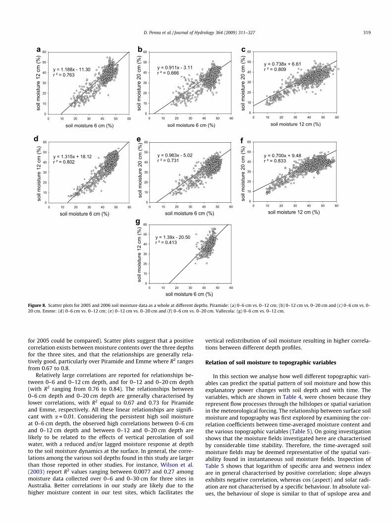
Correlation between point measurements at different depthsare shown as scatter plots in Fig. 8a–g for the three hillslopes (inVallecola only 0–6 cm depth and 0–12 cm depth soil moisture data

Page 9

soil moisture 6 cm (%)0 10 20 30 40 50 60

soil

moi

stur

e 12

cm

(%)

0

10

20

30

40

50

60

y = 1.188x - 11.30r ² = 0.763

soil moisture 6 cm (%)0 10 20 30 40 50 60

soil

moi

stur

e 20

cm

(%)

0

10

20

30

40

50

60

y = 0.911x - 3.11r ² = 0.666

soil moisture 12 cm (%)0 10 20 30 40 50 60

soil

moi

stur

e 20

cm

(%)

0

10

20

30

40

50

60

y = 0.738x + 6.61r ² = 0.809

soil moisture 6 cm (%)0 10 20 30 40 50 60

soil

moi

stur

e 12

cm

(%)

0

10

20

30

40

50

60

y = 1.315x + 18.12r ² = 0.802

soil moisture 6 cm (%)0 10 20 30 40 50 60

soil

moi

stur

e 20

cm

(%)

0

10

20

30

40

50

60

y = 0.963x - 5.02r ² = 0.731

soil moisture 12 cm (%)0 10 20 30 40 50 60

soil

moi

stur

e 20

cm

(%)

0

10

20

30

40

50

60

y = 0.700x + 9.48r ² = 0.833

soil moisture 6 cm (%)0 10 20 30 40 50 60

soil

moi

stur

e 12

cm

(%)

0

10

20

30

40

50

60

y = 1.39x - 20.50r ² = 0.413

a b c

d e f

g

Figure 8. Scatter plots for 2005 and 2006 soil moisture data as a whole at different depths. Piramide: (a) 0–6 cm vs. 0–12 cm; (b) 0–12 cm vs. 0–20 cm and (c) 0–6 cm vs. 0–20 cm. Emme: (d) 0–6 cm vs. 0–12 cm; (e) 0–12 cm vs. 0–20 cm and (f) 0–6 cm vs. 0–20 cm. Vallecola: (g) 0–6 cm vs. 0–12 cm.

D. Penna et al. / Journal of Hydrology 364 (2009) 311–327 319

for 2005 could be compared). Scatter plots suggest that a positivecorrelation exists between moisture contents over the three depthsfor the three sites, and that the relationships are generally rela-tively good, particularly over Piramide and Emme where R2 rangesfrom 0.67 to 0.8.

Relatively large correlations are reported for relationships be-tween 0–6 and 0–12 cm depth, and for 0–12 and 0–20 cm depth(with R2 ranging from 0.76 to 0.84). The relationships between0–6 cm depth and 0–20 cm depth are generally characterised bylower correlations, with R2 equal to 0.67 and 0.73 for Piramideand Emme, respectively. All these linear relationships are signifi-cant with a = 0.01. Considering the persistent high soil moistureat 0–6 cm depth, the observed high correlations between 0–6 cmand 0–12 cm depth and between 0–12 and 0–20 cm depth arelikely to be related to the effects of vertical percolation of soilwater, with a reduced and/or lagged moisture response at depthto the soil moisture dynamics at the surface. In general, the corre-lations among the various soil depths found in this study are largerthan those reported in other studies. For instance, Wilson et al.(2003) report R2 values ranging between 0.0077 and 0.27 amongmoisture data collected over 0–6 and 0–30 cm for three sites inAustralia. Better correlations in our study are likely due to thehigher moisture content in our test sites, which facilitates the

vertical redistribution of soil moisture resulting in higher correla-tions between different depth profiles.

Relation of soil moisture to topographic variables

In this section we analyse how well different topographic vari-ables can predict the spatial pattern of soil moisture and how thisexplanatory power changes with soil depth and with time. Thevariables, which are shown in Table 4, were chosen because theyrepresent flow processes through the hillslopes or spatial variationin the meteorological forcing. The relationship between surface soilmoisture and topography was first explored by examining the cor-relation coefficients between time-averaged moisture content andthe various topographic variables (Table 5). On going investigationshows that the moisture fields investigated here are characterisedby considerable time stability. Therefore, the time-averaged soilmoisture fields may be deemed representative of the spatial vari-ability found in instantaneous soil moisture fields. Inspection ofTable 5 shows that logarithm of specific area and wetness indexare in general characterised by positive correlation; slope alwaysexhibits negative correlation, whereas cos (aspect) and solar radi-ation are not characterised by a specific behaviour. In absolute val-ues, the behaviour of slope is similar to that of upslope area and

Page 10

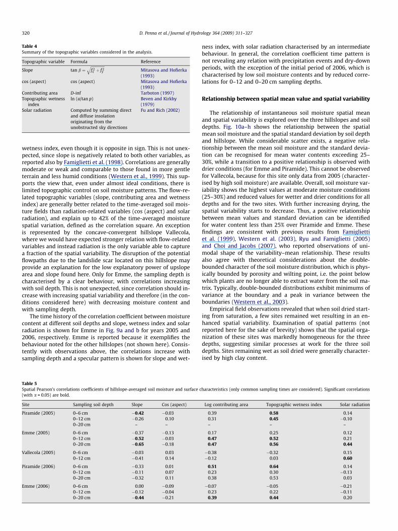
Table 4Summary of the topographic variables considered in the analysis.

Topographic variable Formula Reference

Slope tan b ¼ffiffiffiffiffiffiffiffiffiffiffiffiffiffiffif 2x þ f 2

y

qMitasova and Hofierka(1993)

cos (aspect) cos (aspect) Mitasova and Hofierka(1993)

Contributing area D-inf Tarboton (1997)Topographic wetness

indexln (a/tan p) Beven and Kirkby

(1979)Solar radiation Computed by summing direct

and diffuse insolationoriginating from theunobstructed sky directions

Fu and Rich (2002)

320 D. Penna et al. / Journal of Hydrology 364 (2009) 311–327

wetness index, even though it is opposite in sign. This is not unex-pected, since slope is negatively related to both other variables, asreported also by Famiglietti et al. (1998). Correlations are generallymoderate or weak and comparable to those found in more gentleterrain and less humid conditions (Western et al., 1999). This sup-ports the view that, even under almost ideal conditions, there islimited topographic control on soil moisture patterns. The flow-re-lated topographic variables (slope, contributing area and wetnessindex) are generally better related to the time-averaged soil mois-ture fields than radiation-related variables (cos (aspect) and solarradiation), and explain up to 42% of the time-averaged moisturespatial variation, defined as the correlation square. An exceptionis represented by the concave-convergent hillslope Vallecola,where we would have expected stronger relation with flow-relatedvariables and instead radiation is the only variable able to capturea fraction of the spatial variability. The disruption of the potentialflowpaths due to the landslide scar located on this hillslope mayprovide an explanation for the low explanatory power of upslopearea and slope found here. Only for Emme, the sampling depth ischaracterised by a clear behaviour, with correlations increasingwith soil depth. This is not unexpected, since correlation should in-crease with increasing spatial variability and therefore (in the con-ditions considered here) with decreasing moisture content andwith sampling depth.

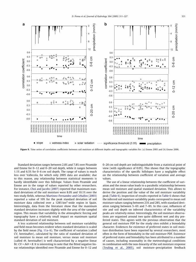
The time history of the correlation coefficient between moisturecontent at different soil depths and slope, wetness index and solarradiation is shown for Emme in Fig. 9a and b for years 2005 and2006, respectively. Emme is reported because it exemplifies thebehaviour noted for the other hillslopes (not shown here). Consis-tently with observations above, the correlations increase withsampling depth and a specular pattern is shown for slope and wet-

Table 5Spatial Pearson’s correlations coefficients of hillslope-averaged soil moisture and surface c(with a = 0.05) are bold.

Site Sampling soil depth Slope Cos (aspect)

Piramide (2005) 0–6 cm �0.42 �0.030–12 cm �0.26 0.100–20 cm – –

Emme (2005) 0–6 cm �0.37 �0.130–12 cm �0.52 �0.030–20 cm �0.65 �0.18

Vallecola (2005) 0–6 cm �0.03 0.030–12 cm �0.41 0.14

Piramide (2006) 0–6 cm �0.33 0.010–12 cm �0.11 0.070–20 cm �0.32 0.11

Emme (2006) 0–6 cm 0.00 �0.090–12 cm �0.12 �0.040–20 cm �0.44 �0.21

ness index, with solar radiation characterised by an intermediatebehaviour. In general, the correlation coefficient time pattern isnot revealing any relation with precipitation events and dry-downperiods, with the exception of the initial period of 2006, which ischaracterised by low soil moisture contents and by reduced corre-lations for 0–12 and 0–20 cm sampling depths.

Relationship between spatial mean value and spatial variability

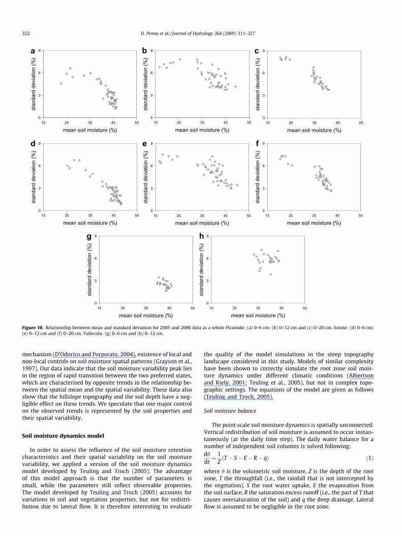
The relationship of instantaneous soil moisture spatial meanand spatial variability is explored over the three hillslopes and soildepths. Fig. 10a–h shows the relationship between the spatialmean soil moisture and the spatial standard deviation by soil depthand hillslope. While considerable scatter exists, a negative rela-tionship between the mean soil moisture and the standard devia-tion can be recognised for mean water contents exceeding 25–30%, while a transition to a positive relationship is observed withdrier conditions (for Emme and Piramide). This cannot be observedfor Vallecola, because for this site only data from 2005 (character-ised by high soil moisture) are available. Overall, soil moisture var-iability shows the highest values at moderate moisture conditions(25–30%) and reduced values for wetter and drier conditions for alldepths and for the two sites. With further increasing drying, thespatial variability starts to decrease. Thus, a positive relationshipbetween mean values and standard deviation can be identifiedfor water content less than 25% over Piramide and Emme. Thesefindings are consistent with previous results from Famigliettiet al. (1999), Western et al. (2003), Ryu and Famiglietti (2005)and Choi and Jacobs (2007), who reported observations of uni-modal shape of the variability–mean relationship. These resultsalso agree with theoretical considerations about the double-bounded character of the soil moisture distribution, which is phys-ically bounded by porosity and wilting point, i.e. the point belowwhich plants are no longer able to extract water from the soil ma-trix. Typically, double-bounded distributions exhibit minimums ofvariance at the boundary and a peak in variance between theboundaries (Western et al., 2003).

Empirical field observations revealed that when soil dried start-ing from saturation, a few sites remained wet resulting in an en-hanced spatial variability. Examination of spatial patterns (notreported here for the sake of brevity) shows that the spatial orga-nization of these sites was markedly homogeneous for the threedepths, suggesting similar processes at work for the three soildepths. Sites remaining wet as soil dried were generally character-ised by high clay content.

haracteristics (only common sampling times are considered). Significant correlations

Log contributing area Topographic wetness index Solar radiation

0.39 0.58 0.140.31 0.45 �0.10– – –

0.17 0.25 0.120.47 0.52 0.210.47 0.56 0.44

�0.38 �0.32 0.15�0.12 0.03 0.60

0.51 0.64 0.140.23 0.30 �0.130.38 0.53 0.03

�0.07 �0.05 �0.210.23 0.22 �0.110.39 0.44 0.20

Page 11

prec

ipita

tion

(mm

/h)

0

4

8

12

-0.6

-0.3

0.0

0.3

0.6

0-6

cm

corre

latio

n co

effic

ient

-0.6

-0.3

0.0

0.3

0.6

0-12

cm

time

28/0

6/05

29

/06/

05

30/0

6/05

01

/07/

05

02/0

7/05

03

/07/

05

04/0

7/05

05

/07/

05

06/0

7/05

07

/07/

05

08/0

7/05

09

/07/

05

10/0

7/05

11

/07/

05

12/0

7/05

13

/07/

05

14/0

7/05

15

/07/

05

16/0

7/05

17

/07/

05

18/0

7/05

19

/07/

05

20/0

7/05

21

/07/

05

-0.6

-0.3

0.0

0.3

0.6

0-20

cm

prec

ipita

tion

(mm

/h)

0

4

8

12

-0.6

-0.3

0.0

0.3

0.6

0-6

cm

corre

latio

n co

effic

ient

-0.6

-0.3

0.0

0.3

0.6

0-12

cm

time

21/0

6/06

22

/06/

06

23/0

6/06

24

/06/

06

25/0

6/06

26

/06/

06

27/0

6/06

28

/06/

06

29/0

6/06

30

/06/

06

01/0

7/06

02

/07/

06

03/0

7/06

04

/07/

06

05/0

7/06

06

/07/

06

07/0

7/06

08

/07/

06

09/0

7/06

10

/07/

06

11/0

7/06

12

/07/

06

13/0

7/06

14

/07/

06

15/0

7/06

16

/07/

06

-0.6

-0.3

0.0

0.3

0.6

0-20

cm

a b

Figure 9. Time series of correlation coefficients between soil moisture at different depths and topographic variables for: (a) Emme 2005 and (b) Emme 2006.

D. Penna et al. / Journal of Hydrology 364 (2009) 311–327 321

Standard deviation ranges between 2.8% and 7.8% over Piramideand Emme for 0–12 and 0–20 soil depth, while it ranges between1.1% and 6.5% for 0–6 cm soil depth. The range of values is muchless over Vallecola, for which only 2005 data are available; dueto this reason, any relationship between statistical moments ishardly identifiable over this hillslope. Values from Piramide andEmme are in the range of values reported by other researchers.For instance, Choi and Jacobs (2007) reported that maximum stan-dard deviations of the soil moisture were 8.0% and 10.1% over thetwo study fields, whereas Martinez-Fernandez and Ceballos (2003)reported a value of 10% for the peak standard deviation of soilmoisture data collected over a 1285 km2-wide region in Spain.Interestingly, data from the literature show that the maximumstandard deviation increases slightly with the area of the sampledregion. This means that variability in the atmospheric forcing andtopography have a relatively small impact on maximum spatialstandard deviation of soil moisture.

A less scattered relationship between soil moisture variabilityand field mean becomes evident when standard deviation is scaledby the field mean (Fig. 11a–h). The coefficient of variation (calledCV, hereinafter), calculated by the ratio of standard deviation ofsoil moisture to mean soil moisture, versus mean soil moisture(called H, hereinafter) is well characterised by a negative linearfit: CV = AH + B. It is interesting to note that the fitted negative lin-ear relationships identified over Piramide and Emme for 0–12 and

0–20 cm soil depth are indistinguishable from a statistical point ofview (with significance of 0.05). This shows that the topographiccharacteristics of the specific hillslopes have a negligible effecton the relationship between coefficient of variation and averagevalues.

The use of a linear relationship between the coefficient of vari-ation and the mean value leads to a parabolic relationship betweenmean soil moisture and spatial standard deviation. This allows toderive the position and the value of the soil moisture variabilitypeak (Table 6). Inspection of results reported in Table 6 shows thatthe inferred soil moisture variability peaks correspond to mean soilmoisture values ranging between 23% and 28%, with standard devi-ation ranging between 5–6% and 7–8%. In this case, influences ofsite and soil depth on inferred characteristics of the variabilitypeaks are relatively minor. Interestingly, the soil moisture observa-tions are organised around two quite different wet and dry pre-ferred states. This agrees with the previous observation that thegeneral soil moisture PDF for the study sites exhibit a bimodalitycharacter. Evidences for existence of preferred states in soil mois-ture distribution have been reported by several researchers, mostoften in the form of bimodality in the soil moisture PDF. Existenceof preferred states and bimodality has been attributed to a numberof causes, including seasonality in the meteorological conditionsin combination with the non-linearity of the soil moisture response(Teuling et al., 2005), soil moisture–precipitation feedback

Page 12

mean soil moisture (%)15 25 35 45 55

stan

dard

dev

iatio

n (%

)

0

3

6

9

mean soil moisture (%)15 25 35 45 55

stan

dard

dev

iatio

n (%

)

0

3

6

9

mean soil moisture (%)15 25 35 45 55

stan

dard

dev

iatio

n (%

)

0

3

6

9

mean soil moisture (%)15 25 35 45 55

stan

dard

dev

iatio

n (%

)

0

3

6

9

mean soil moisture (%)15 25 35 45 55

stan

dard

dev

iatio

n (%

)

0

3

6

9

mean soil moisture (%)15 25 35 45 55

stan

dard

dev

iatio

n (%

)

0

3

6

9

mean soil moisture (%)15 25 35 45 55

stan

dard

dev

iatio

n (%

)

0

3

6

9

mean soil moisture (%)15 25 35 45 55

stan

dard

dev

iatio

n (%

)

0

3

6

9

a b c

d e f

g h

Figure 10. Relationship between mean and standard deviation for 2005 and 2006 data as a whole Piramide: (a) 0–6 cm; (b) 0–12 cm and (c) 0–20 cm. Emme: (d) 0–6 cm;(e) 0–12 cm and (f) 0–20 cm. Vallecola: (g) 0–6 cm and (h) 0–12 cm.

322 D. Penna et al. / Journal of Hydrology 364 (2009) 311–327

mechanism (D’Odorico and Porporato, 2004), existence of local andnon-local controls on soil moisture spatial patterns (Grayson et al.,1997). Our data indicate that the soil moisture variability peak liesin the region of rapid transition between the two preferred states,which are characterised by opposite trends in the relationship be-tween the spatial mean and the spatial variability. These data alsoshow that the hillslope topography and the soil depth have a neg-ligible effect on these trends. We speculate that one major controlon the observed trends is represented by the soil properties andtheir spatial variability.

Soil moisture dynamics model

In order to assess the influence of the soil moisture retentioncharacteristics and their spatial variability on the soil moisturevariability, we applied a version of the soil moisture dynamicsmodel developed by Teuling and Troch (2005). The advantageof this model approach is that the number of parameters issmall, while the parameters still reflect observable properties.The model developed by Teuling and Troch (2005) accounts forvariations in soil and vegetation properties, but not for redistri-bution due to lateral flow. It is therefore interesting to evaluate

the quality of the model simulations in the steep topographylandscape considered in this study. Models of similar complexityhave been shown to correctly simulate the root zone soil mois-ture dynamics under different climatic conditions (Albertsonand Kiely, 2001; Teuling et al., 2005), but not in complex topo-graphic settings. The equations of the model are given as follows(Teuling and Troch, 2005).

Soil moisture balance

The point scale soil moisture dynamics is spatially unconnected.Vertical redistribution of soil moisture is assumed to occur instan-taneously (at the daily time step). The daily water balance for anumber of independent soil columns is solved following:dhdt¼ 1

ZðT � S� E� R� qÞ ð1Þ

where h is the volumetric soil moisture, Z is the depth of the rootzone, T the throughfall (i.e., the rainfall that is not intercepted bythe vegetation), S the root water uptake, E the evaporation fromthe soil surface, R the saturation excess runoff (i.e., the part of T thatcauses oversaturation of the soil) and q the deep drainage. Lateralflow is assumed to be negligible in the root zone.

Page 13

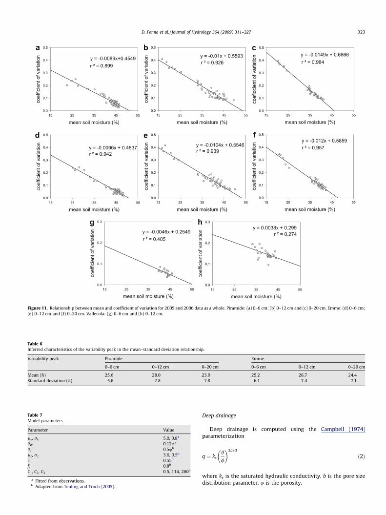
Table 7Model parameters.

Parameter Value

lk, rk 5.0, 0.8a

hW 0.12ua

hc 0.5ub

ln, rn 3.6, 0.5b

c 0.55b

fr 0.8b

C1, C2, C3 0.5, 114, 260b

a Fitted from observations.b Adapted from Teuling and Troch (2005).

mean soil moisture (%)15 25 35 45 55

coef

ficie

nt o

f var

iatio

n

0.0

0.1

0.2

0.3

0.4

0.5

r ² = 0.899y = -0.0089x+0.4549

mean soil moisture (%)15 25 35 45 55

coef

ficie

nt o

f var

iatio

n

0.0

0.1

0.2

0.3

0.4

0.5

r ² = 0.926y = -0.01x + 0.5593

mean soil moisture (%)15 25 35 45 55

coef

icci

ent o

f var

iatio

n

0.0

0.1

0.2

0.3

0.4

0.5

r ² = 0.984y = -0.0149x + 0.6866

mean soil moisture (%)15 25 35 45 55

coef

ficie

nt o

f var

iatio

n

0.0

0.1

0.2

0.3

0.4

0.5

r ² = 0.942y = -0.0096x + 0.4837

mean soil moisture (%)15 25 35 45 55

coef

ficie

nt o

f var

iatio

n

0.0

0.1

0.2

0.3

0.4

0.5

r ² = 0.939y = -0.0104x + 0.5546

mean soil moisture (%)15 25 35 45 55

coef

ficie

nt o

f var

iatio

n

0.0

0.1

0.2

0.3

0.4

0.5

r ² = 0.957y = -0.012x + 0.5859

mean soil moisture (%)15 25 35 45 55

coef

ficie

nt o

f var

iatio

n

0.0

0.1

0.2

0.3

r ² = 0.405y = -0.0046x + 0.2549

mean soil moisture (%)15 25 35 45 55

coef

ficie

nt o

f var

iatio

n

0.0

0.1

0.2

0.3

r ² = 0.274y = 0.0038x + 0.299

a b c

d e f

g h

Figure 11. Relationship between mean and coefficient of variation for 2005 and 2006 data as a whole. Piramide: (a) 0–6 cm; (b) 0–12 cm and (c) 0–20 cm. Emme: (d) 0–6 cm;(e) 0–12 cm and (f) 0–20 cm. Vallecola: (g) 0–6 cm and (h) 0–12 cm.

Table 6Inferred characteristics of the variability peak in the mean–standard deviation relationship.

Variability peak Piramide Emme

0–6 cm 0–12 cm 0–20 cm 0–6 cm 0–12 cm 0–20 cm

Mean (%) 25.6 28.0 23.0 25.2 26.7 24.4Standard deviation (%) 5.6 7.8 7.8 6.1 7.4 7.1

D. Penna et al. / Journal of Hydrology 364 (2009) 311–327 323

Deep drainage

Deep drainage is computed using the Campbell (1974)parameterization

q ¼ ksh/

� �2bþ3

ð2Þ

where ks is the saturated hydraulic conductivity, b is the pore sizedistribution parameter, u is the porosity.

Page 14

time

21/6

/06

22

/6/0

6

23/6

/06

24

/6/0

6

25/6

/06

26

/6/0

6

27/6

/06

28

/6/0

6

29/6

/06

30

/6/0

6

1/7/

06

2/7/

06

3/7/

06

4/7/

06

5/7/

06

6/7/

06

7/7/

06

8/7/

06

9/7/

06

10/7

/06

11

/7/0

6

12/7

/06

13

/7/0

6

14/7

/06

15

/7/0

6

16/7

/06

stan

dard

dev

iatio

n (%

) mea

n so

il m

oist

ure

(%)

2

4

6

8

observed SD simulated SD

20

30

40

50

60

prec

ipita

tion

(mm

/h)

0

5

10

15

20

observed meansimulated mean

time21

/6/0

6

22/6

/06

23

/6/0

6

24/6

/06

25

/6/0

6

26/6

/06

27

/6/0

6

28/6

/06

29

/6/0

6

30/6

/06

1/

7/06

2/

7/06

3/

7/06

4/

7/06

5/

7/06

6/

7/06

7/

7/06

8/

7/06

9/

7/06

10

/7/0

6

11/7

/06

12

/7/0

6

13/7

/06

14

/7/0

6

15/7

/06

16

/7/0

6

stan

dard

dev

iatio

n (%

) mea

n so

il m

oist

ure

(%)

2

4

6

8observed SD simulated SD

20

30

40

50

60

prec

ipita

tion

(mm

/h)

0

5

10

15

20

observed meansimulated mean

a b

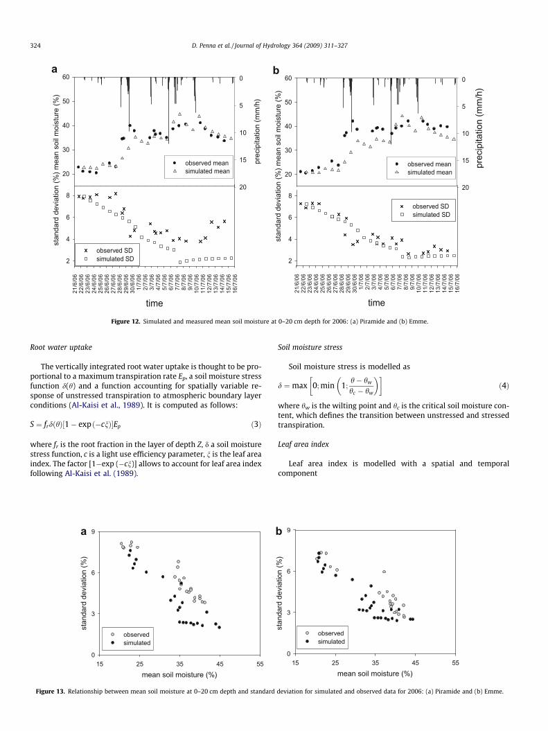
Figure 12. Simulated and measured mean soil moisture at 0–20 cm depth for 2006: (a) Piramide and (b) Emme.

324 D. Penna et al. / Journal of Hydrology 364 (2009) 311–327

Root water uptake

The vertically integrated root water uptake is thought to be pro-portional to a maximum transpiration rate Ep, a soil moisture stressfunction d(h) and a function accounting for spatially variable re-sponse of unstressed transpiration to atmospheric boundary layerconditions (Al-Kaisi et al., 1989). It is computed as follows:

S ¼ frdðhÞ½1� exp ð�cnÞ�Ep ð3Þ

where fr is the root fraction in the layer of depth Z, d a soil moisturestress function, c is a light use efficiency parameter, n is the leaf areaindex. The factor [1�exp (�cn)] allows to account for leaf area indexfollowing Al-Kaisi et al. (1989).

mean soil moisture (%)15 25 35 45 55

stan

dard

dev

iatio

n (%

)

0

3

6

9

observedsimulated

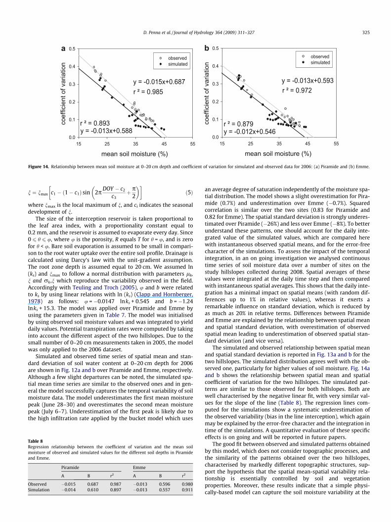
a b

Figure 13. Relationship between mean soil moisture at 0–20 cm depth and standard

Soil moisture stress

Soil moisture stress is modelled as

d ¼max 0; min 1;h� hw

hc � hw

� �� �ð4Þ

where hw is the wilting point and hc is the critical soil moisture con-tent, which defines the transition between unstressed and stressedtranspiration.

Leaf area index

Leaf area index is modelled with a spatial and temporalcomponent

mean soil moisture (%)15 25 35 45 55

stan

dard

dev

iatio

n (%

)

0

3

6

9

observedsimulated

deviation for simulated and observed data for 2006: (a) Piramide and (b) Emme.

Page 15

mean soil moisture (%)15 25 35 45 55

coef

ficie

nt o

f var

iatio

n

0.0

0.1

0.2

0.3

0.4

0.5

observedsimulated

r ² = 0.985y = -0.015x+0.687

y = -0.013x+0.588r ² = 0.893

mean soil moisture (%)15 25 35 45 55

coef

ficie

nt o

f var

iatio

n

0.0

0.1

0.2

0.3

0.4

0.5observedsimulated

y = -0.013x+0.593r ² = 0.972

r ² = 0.879y = -0.012x+0.546

a b

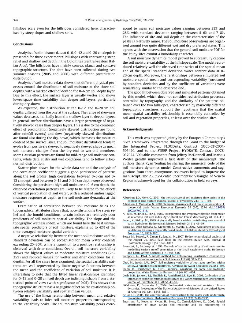
Figure 14. Relationship between mean soil moisture at 0–20 cm depth and coefficient of variation for simulated and observed data for 2006: (a) Piramide and (b) Emme.

D. Penna et al. / Journal of Hydrology 364 (2009) 311–327 325

n ¼ nmax c1 � 1� c1ð Þ sin 2pDOY � c2

c3þ p

2

� �� �ð5Þ

where nmax is the local maximum of n, and ci indicates the seasonaldevelopment of n.

The size of the interception reservoir is taken proportional tothe leaf area index, with a proportionality constant equal to0.2 mm, and the reservoir is assumed to evaporate every day. Since0 6 h 6 u, where u is the porosity, R equals T for h = u, and is zerofor h < u. Bare soil evaporation is assumed to be small in compari-son to the root water uptake over the entire soil profile. Drainage iscalculated using Darcy’s law with the unit-gradient assumption.The root zone depth is assumed equal to 20 cm. We assumed ln(ks) and nmax to follow a normal distribution with parameters lk,n and rk,n which reproduce the variability observed in the field.Accordingly with Teuling and Troch (2005), u and b were relatedto ks by using linear relations with ln (ks) (Clapp and Hornberger,1978) as follows: u = �0.0147 lnks + 0.545 and b = �1.24lnks + 15.3. The model was applied over Piramide and Emme byusing the parameters given in Table 7. The model was initialisedby using observed soil moisture values and was integrated to yielddaily values. Potential transpiration rates were computed by takinginto account the different aspect of the two hillslopes. Due to thesmall number of 0–20 cm measurements taken in 2005, the modelwas only applied to the 2006 dataset.

Simulated and observed time series of spatial mean and stan-dard deviation of soil water content at 0–20 cm depth for 2006are shown in Fig. 12a and b over Piramide and Emme, respectively.Although a few slight departures can be noted, the simulated spa-tial mean time series are similar to the observed ones and in gen-eral the model successfully captures the temporal variability of soilmoisture data. The model underestimates the first mean moisturepeak (June 28–30) and overestimates the second mean moisturepeak (July 6–7). Underestimation of the first peak is likely due tothe high infiltration rate applied by the bucket model which uses

Table 8Regression relationship between the coefficient of variation and the mean soilmoisture of observed and simulated values for the different soil depths in Piramideand Emme.

Piramide Emme

A B r2 A B r2

Observed �0.015 0.687 0.987 �0.013 0.596 0.980Simulation �0.014 0.610 0.897 �0.013 0.557 0.911

an average degree of saturation independently of the moisture spa-tial distribution. The model shows a slight overestimation for Pira-mide (0.7%) and underestimation over Emme (�0.7%). Squaredcorrelation is similar over the two sites (0.83 for Piramide and0.82 for Emme). The spatial standard deviation is strongly underes-timated over Piramide (�26%) and less over Emme (�8%). To betterunderstand these patterns, one should account for the daily inte-grated value of the simulated values, which are compared herewith instantaneous observed spatial means, and for the error-freecharacter of the simulations. To assess the impact of the temporalintegration, in an on going investigation we analysed continuoustime series of soil moisture data over a number of sites on thestudy hillslopes collected during 2008. Spatial averages of thesevalues were integrated at the daily time step and then comparedwith instantaneous spatial averages. This shows that the daily inte-gration has a minimal impact on spatial means (with random dif-ferences up to 1% in relative values), whereas it exerts aremarkable influence on standard deviation, which is reduced byas much as 20% in relative terms. Differences between Piramideand Emme are explained by the relationship between spatial meanand spatial standard deviation, with overestimation of observedspatial mean leading to underestimation of observed spatial stan-dard deviation (and vice versa).

The simulated and observed relationship between spatial meanand spatial standard deviation is reported in Fig. 13a and b for thetwo hillslopes. The simulated distribution agrees well with the ob-served one, particularly for higher values of soil moisture. Fig. 14aand b shows the relationship between spatial mean and spatialcoefficient of variation for the two hillslopes. The simulated pat-terns are similar to those observed for both hillslopes. Both arewell characterised by the negative linear fit, with very similar val-ues for the slope of the line (Table 8). The regression lines com-puted for the simulations show a systematic underestimation ofthe observed variability (bias in the line interception), which againmay be explained by the error-free character and the integration intime of the simulations. A quantitative evaluation of these specificeffects is on going and will be reported in future papers.

The good fit between observed and simulated patterns obtainedby this model, which does not consider topographic processes, andthe similarity of the patterns obtained over the two hillslopes,characterised by markedly different topographic structures, sup-port the hypothesis that the spatial mean-spatial variability rela-tionship is essentially controlled by soil and vegetationproperties. Moreover, these results indicate that a simple physi-cally-based model can capture the soil moisture variability at the

Page 16

326 D. Penna et al. / Journal of Hydrology 364 (2009) 311–327

hillslope scale even for the hillslopes considered here, character-ised by steep slopes and shallow soils.

Conclusions

Analysis of soil moisture data at 0–6, 0–12 and 0–20 cm depth ispresented for three experimental hillslopes with contrasting steeprelief and shallow soil depth in the Dolomites (central-eastern Ital-ian Alps). The hillslopes have mainly convex, planar and concavetopographic structure. The data have been collected during twosummer seasons (2005 and 2006) with different precipitationdistribution.

Analysis of soil moisture data shows that different physical pro-cesses control the distribution of soil moisture at the three soildepths, with a marked effect of dew on the 0–6 cm soil depth layer.Due to this effect, the surface layer is usually wetter and showslower space–time variability than deeper soil layers, particularlyduring dry-down.

As expected, the distribution at the 0–12 and 0–20 cm soildepths differed from the one at the surface. The range of skewnessvalues decreases markedly from the shallow layer to deeper layers.In general, surface distributions have a larger percentage of nega-tively skewed cases than deeper layers. This is due to the combinedeffect of precipitation (negatively skewed distribution are foundafter rainfall events) and dew (negatively skewed distributionsare found also during the dry-down) which increases the moisturecontent of the surface layer. The soil moisture distribution tends toevolve from positively skewed to negatively skewed shape as meansoil moisture changes from the dry-end to wet-end members.More Gaussian patterns are found for mid-range soil moisture con-tents, while data at dry and wet conditions tend to follow a log–normal distribution.

Scatter plots drawn for the whole data set and the analysis ofthe correlation coefficient suggest a good persistence of patternsalong the soil profile: high correlations between 0–6 cm and 0–12 cm depth and between 0–12 and 0–20 cm depth were observed.Considering the persistent high soil moisture at 0–6 cm depth, theobserved correlation patterns are likely to be related to the effectsof vertical percolation of soil water, with a reduced and/or laggedmoisture response at depth to the soil moisture dynamics at thesurface.

Examination of correlation between soil moisture fields andtopographical attributes shows that, notwithstanding the steep re-lief and the humid conditions, terrain indices are relatively poorpredictors of soil moisture spatial variability. The slope and thetopographic wetness index, which are found here the best univar-iate spatial predictors of soil moisture, explains up to 42% of thetime-averaged moisture spatial variation.

A negative relationship between the mean soil moisture and thestandard deviation can be recognised for mean water contentsexceeding 25–30%, while a transition to a positive relationship isobserved with drier conditions. Overall, soil moisture variabilityshows the highest values at moderate moisture conditions (25–35%) and reduced values for wetter and drier conditions for alldepths. For all the cases here examined, the spatial variability pat-terns are well represented by linear negative functions betweenthe mean and the coefficient of variation of soil moisture. It isinteresting to note that the fitted linear relationships identifiedfor 0–12 and 0–20 cm soil depth are indistinguishable from a sta-tistical point of view (with significance of 0.05). This shows thattopographic structure has a negligible effect on the relationship be-tween relative variability and spatial mean values.

The use of the linear relationship between mean and relativevariability leads to infer soil moisture properties correspondingto the variability peaks. The soil moisture variability peaks corre-

spond to mean soil moisture values ranging between 23% and28%, with standard deviation ranging between 5–6% and 7–8%.The influence of site and soil depth on the characteristics of thepeaks is relatively minor. The soil moisture observations are organ-ised around two quite different wet and dry preferred states. Thisagrees with the observation that the general soil moisture PDF forthe study sites exhibit a bimodality character.

A soil moisture dynamics model proved to successfully capturethe soil moisture variability at the hillslope scale. The model repro-duced relatively well the observed time series of the spatial meanand of the spatial standard deviation water content data at 0–20 cm depth. Moreover, the relationships between simulated soilmoisture spatial mean and corresponding variability (measuredby standard deviation and by the coefficient of variation) wereremarkably similar to the observed one.

The good fit between observed and simulated patterns obtainedby this model, which does not consider redistribution processescontrolled by topography, and the similarity of the patterns ob-tained over the two hillslopes, characterised by markedly differenttopographic structures, support the hypothesis that the spatialmean-spatial variability relationship is essentially controlled bysoil and vegetation properties, at least over the studied sites.

Acknowledgments

This work was supported jointly by the European Community’sSixth Framework Programme through the Grant to the budget ofthe Integrated Project FLOODsite, Contract GOCE-CT-2004-505420, and to the STREP Project HYDRATE, Contract GOCE-037024. Valuable comments from Jeffrey McDonnell and MarkusWeiler greatly improved a first draft of the manuscript. Theauthors thank Ryan Teuling for sharing the numerical code of thesoil moisture dynamics model. Constructive comments and sug-gestions from three anonymous reviewers helped to improve themanuscript. The ARPAV-Centro Sperimentale Valanghe of VenetoRegion is acknowledged for the collaboration in field surveys.

References

Albertson, J.D., Kiely, G., 2001. On the structure of soil moisture time series in thecontext of land surface models. Journal of Hydrology 243, 101–119.

Albertson, J., Montaldo, N., 2003. Temporal dynamics of soil moisture variability: 1.theoretical basis. Water Resources Research 39 (10), 1274. doi:10.1029/2002WR001616.

Al-Kaisi, M., Brun, L., Enz, J., 1989. Transpiration and evapotranspiration from maizeas related to leaf area index. Agricultural and Forest Meteorology 48, 111–116.

Beven, K., Kirkby, M., 1979. A physically based variable contributing area model ofbasin hydrology. Hydrological Sciences Bulletin 24 (1), 43–69.

Borga, M., Dalla Fontana, G., Gregoretti, C., Marchi, L., 2002. Assessment of shallowlandsliding by using a physically based model of hillslope stability. HydrologicalProcesses 16, 2833–2851.

Borga, M., Boscolo, P., Zanon, F., Sangati, M., 2007. Hydrometeorological analysis ofthe August 29, 2003 flash flood in the eastern Italian Alps. Journal ofHydrometeorology 8 (5), 1049–1067.

Bronstert, A., Bárdossy, A., 1999. The role of spatial variability of soil moisture formodelling surface runoff generation at the small catchment scale. Hydrologyand Earth System Sciences 3 (4), 505–516.

Campbell, G., 1974. A simple method for determining unsaturated conductivityfrom moisture retention data. Soil Science 117 (6), 311–314.

Choi, M., Jacobs, J.M., 2007. Soil moisture variability of root zone profiles withinSMEX02 remote sensing footprints. Advances in Water Resources 30, 883–896.

Clapp, R., Hornberger, G., 1978. Empirical equations for some soil hydraulicproperties. Water Resources Research 14 (4), 601–604.

Cosh, M.H., Jackson, T.J., Bindlish, R., Famiglietti, J.S., Ryu, D., 2005. Calibration of animpedance probe for estimation of surface soil water content over large regions.Journal of Hydrology 311 (2005), 49–58.

D’Odorico, P., Porporato, A., 2004. Preferential states in soil moisture climatedynamics. Proceeding of the National Academy of Sciences of the United Statesof America 101 (24), 8848–8851.

de Jong, C., 2005. The contribution of condensation to the water cycle under high-mountain conditions. Hydrological Processes 19 (12), 2419–2435.

Engstrom, R., Hope, A., Kwon, H., Stow, D., Zamolodchikov, D., 2005. Spatialdistribution of near surface soil moisture and its relationship to

Page 17

D. Penna et al. / Journal of Hydrology 364 (2009) 311–327 327

microtopography in the Alaskan Arctic coastal plain. Nordic Hydrology 36, 219–234.

Famiglietti, J.S., Rudnicki, J.W., Rodell, M., 1998. Variability in surface soil moisturecontent along a hillslope transect: Rattlesnake Hill, Texas. Journal of Hydrology210, 259–281.

Famiglietti, J.S., Devereaux, J.A., Laymon, C.A., Tsegaye, T., Houser, P.R., Jackson, T.J.,1999. Ground-based investigation of soil moisture variability within remotesensing footprints during the Southern Great Plains 1997 (SGP97) HydrologyExperiment. Water Resources Research 35 (6), 1839–1851.

Famiglietti, J.S., Ryu, D., Berg, A.A., Rodell, M., Jackson, T.J., 2008. Field observationsof soil moisture variability across scales. Water Resources Research 44,W01423. doi:10.1029/2006WR005804.

Fu, P., Rich, P.M., 2002. A geometric solar radiation model with applications inagriculture and forestry. Computers and Electronics in Agriculture 37, 25–35.

Gaskin, G.J., Miller, J.D., 1996. Measurement of soil water content using a simplifiedimpedance measuring technique. Journal of Agricultural Engineering Research63, 153–160.

Grant, L., Seyfried, M., McNamara, J., 2004. Spatial variation and temporal stabilityof soil water in a snow-dominated, mountain catchment. HydrologicalProcesses 18 (18), 3493–3511.

Grayson, R.B., Western, A.W., 2001. Terrain and the distribution of soil moisture.Hydrological Processes 15, 2689–2690.

Grayson, R.B., Western, A.W., Chiew, F.H.S., Blöschl, G., 1997. Preferred states inspatial soil moisture patterns: local and non local controls. Water ResourcesResearch 33 (12), 2897–2908.

Kaleita, A.L., Heitman, J.L., Logsdon, D.D., 2005. Field calibration of the Theta Probefor Des Moines Lobe soils. Applied Engineering in Agriculture 21 (5), 865–870.

Koster, R.D., Dirmeyer, P.A., Guo, Z., Bonan, G., Chan, E., Cox, P., Gordon, C.T., Kanae,S., Kowalczyk, E., Lawrence, D., Liu, P., Lu, C.-H., Malyshev, S., McAvaney, B.,Mitchell, K., Mocko, D., Oki, T., Oleson, K., Pitman, A., Sud, Y.C., Taylor, C.M.,Verseghy, D., Vasic, R., Xue, Y., Yamada, T., 2004. Regions of strong couplingbetween soil moisture and precipitation. Science 305, 1138–1140.

Looney, S.W., Gulledge, T.R., 1985. Probability plotting positions and goodness of fitfor the normal distribution. The Statistician 34, 297–303.

Martinez-Fernandez, J., Ceballos, A., 2003. Temporal stability of soil moisture in alarge-field experiment in Spain. Soil Science Society of America Journal 67,1647–1656.

Miller, J.D., Gaskin, G.J., Anderson, H., 1997. From drought to flood: catchmentresponses revealed using novel soil water probes. Hydrological Processes 11,533–541.

Mitasova, H., Hofierka, J., 1993. Interpolation by regularized spline with tension II,application to terrain modeling and surface geometry analysis. MathematicalGeology 25, 657–669.

Mohanty, B.P., Skaggs, T.H., 2001. Spatio–temporal evolution and time-stablecharacteristics of soil moisture within remote sensing footprints with varyingsoil, slope, and vegetation. Advances in Water Resources 24, 1051–1067.

Monteith, J.L., 1965. Evaporation and the environment. Symposia of the Society forExperimental Biology 19, 205–234.

Norbiato, D., Borga, M., 2008. Analysis of hysteretic behaviour of a hillslope-storagekinematic wave model for subsurface flow. Advances in Water Resources 31,118–131.

Norbiato, D., Borga, M., Merz, R., Blöschl, G., Carton, A., 2008. Flash flood warningbased on rainfall depth-duration thresholds and soil moisture conditions: anassessment for gauged and ungauged basins. Journal of Hydrology, 274–290.doi:10.1016/j.jhydrol.2008.08.023.

Pan, F., Peters-Lidard, C.D., Sale, M.J., 2003. An analytical method for predictingsurface soil moisture from rainfall observations. Water Resources Research 39(11), 1314. doi:10.1029/2003WR002142.

Porporato, A., Daly, E., Rodríguez-Iturbe, I., 2004. Soil water balance and ecosystemresponse to climate change. American Naturalist 164 (5), 625–633.

Raats, P.A.C., 2001. Developments in soil–water physics since the mid 1960s.Geoderma 100, 355–387.

Rodríguez-Iturbe, I., Porporato, A., 2004. Ecohydrology of Water-controlledEcosystems: Soil Moisture and Plant Dynamics. Cambridge University Press,Cambridge, UK.

Ryu, D.R., Famiglietti, J.S., 2005. Characterization of footprint-scale surface soilmoisture variability using gaussian and beta distribution function during theSouthern Great Plains 1997 (SGP97) hydrology experiment. Water ResourcesResearch 41 (12), W12433. doi:10.1029/2004WR003835.

Salvucci, G.D., 1998. Limiting relations between soil moisture and soil texture withimplications for measured, modeled and remotely sensed estimates.Geophysical Research Letters 25 (10), 1757–1760.

Silverman, B.W., 1986. Density Estimation for Statistics and Data Analysis. Chapman& Hall, London.

Stenger, R., Barkle, G., Burgess, C., 2005. Laboratory calibrations of water contentreflectometers and their in-situ verification. Australian Journal of Soil Research43 (5), 607–615.

Tarboton, D.G., 1997. A new method for the determination of flow directions andupslope area in grid digital elevation models. Water Resources Research 33 (2),309–319.

Teuling, A.J., Troch, P.A., 2005. Improved understanding of soil moisture variabilitydynamics. Geophysical Research Letters 32, L05404. doi:10.1029/2004GL021935.

Teuling, A.J., Uijlenhoet, R., Troch, P.A., 2005. On bimodality in warm season soilmoisture observations. Geophysical Research Letters 32, L13402. doi:10.1029/2005GL023223.

Vereecken, H., Kamai, T., Harter, T., Kasteel, R., Hopmans, J., Vanderborght, J., 2007.Explaining soil moisture variability as a function of mean soil moisture: astochastic unsaturated flow perspective. Geophysical Research Letters 34,L22402. doi:10.1029/2007GL031813.

Vogel, R.M., 1986. The probability plot correlation coefficient test for normal,lognormal, and Gumbel distributions. Water Resources Research 22, 587–590.

Walker, J.P., Willgoose, G.R., Kalma, J.D., 2004. In situ measurement of soil moisture:a comparison of techniques. Journal of Hydrology 293, 85–99.

Western, A.W., Grayson, R.B., 1998. The Tarrawarra data set: soil moisture patterns,soil characteristics and hydrological flux measurements. Water ResourcesResearch 34 (10), 2765–2768.

Western, A.W., Grayson, R.B., 2000. Soil moisture and runoff processes atTarrawarra. In: Grayson, R., Blöschl, G. (Eds.), Spatial Patterns in CatchmentHydrology: Observation and Modelling. Cambridge University Press,Cambridge.

Western, A.W., Grayson, R.B., Blöschl, G., Willgoose, G.R., McMahon, A., 1999.Observed spatial organization of soil moisture and its relation to terrain indices.Water Resources Research 35 (3), 797–810.

Western, A.W., Richter, H., Chiew, F.H.S., Young, R.I., Mills, G., Grayson, R.B., Manton,M., McMahon, T.A., 2002. Testing the Australian Bureau of Meteorology’s landsurface scheme using soil moisture observations from the Murrumbidgeecatchment. In: Hydrology and Water Resources Symposium, July, 2002.

Western, A.W., Grayson, R.B., Blöschl, G., Wilson, D.J., 2003. Spatial variability of soilmoisture and its implications for scaling. In: Perchepsky, Y., Selim, M., Radcliffe,A. (Eds.), Scaling Methods in Soil Physics. CRC Press, Boca Raton, pp. 119–142.

Western, A.W., Zhou, S., Grayson, R.B., McMahon, T.A., Blöschl, G., Wilson, D.J., 2004.Spatial correlation of soil moisture in small catchments and its relationship todominant spatial hydrological processes. Journal of Hydrology 286, 113–134.

Wilson, J.D., Western, A.W., Grayson, R.B., Berg, A.A., Lear, M.S., Rodell, M.,Famiglietti, J.S., Wood, R.A., McMahon, A.T., 2003. Spatial distribution of soilmoisture over 6 and 30 cm depth, Mahurangi river catchment, New Zealand.Journal of Hydrology 276, 254–274.

Wilson, J.D., Western, A.W., Grayson, R.B., 2004. Identifying and quantifying sourcesof variability in temporal and spatial soil moisture observations. WaterResources Research 40, W02507.