Hillslope hydrologic connectivity controls riparian groundwater turnover: Implications of catchment structure for riparian buffering and stream water sources

Hillslope hydrologic connectivity controls riparian groundwaterturnover: Implications of catchment structure for riparianbuffering and stream water sources

Kelsey G. Jencso,1 Brian L. McGlynn,1 Michael N. Gooseff,2 Kenneth E. Bencala,3

and Steven M. Wondzell4

Received 27 October 2009; revised 7 March 2010; accepted 18 May 2010; published 15 October 2010.

[1] Hydrologic connectivity between catchment upland and near stream areas is essentialfor the transmission of water, solutes, and nutrients to streams. However, our currentunderstanding of the role of riparian zones in mediating landscape hydrologic connectivityand the catchment scale export of water and solutes is limited. We tested therelationship between the duration of hillslope!riparian!stream (HRS) hydrologicconnectivity and the rate and degree of riparian shallow groundwater turnover along fourHRS well transects within a set of nested mountain catchments (Tenderfoot CreekExperimental Forest, MT). Transect HRSwater table connectivity ranged from 9 to 123 daysduring the annual snowmelt hydrograph. Hillslope water was always characterized bylow specific conductance (!27 mS cm"1). In transects with transient hillslope watertables, riparian groundwater specific conductance was elevated during base flowconditions (!127 mS cm"1) but shifted toward hillslope signatures once a HRSgroundwater connection was established. The degree of riparian groundwater turnoverwas proportional to the duration of HRS connectivity and inversely related to theriparian: hillslope area ratios (buffer ratio; r2 = 0.95). We applied this relationship to thestream network in seven subcatchments within the Tenderfoot Creek ExperimentalForest and compared their turnover distributions to source water contributions measuredat each catchment outlet. The amount of riparian groundwater exiting each of the sevencatchments was linearly related (r2 = 0.92) to their median riparian turnover time. Ourobservations suggest that the size and spatial arrangement of hillslope and riparian zonesalong a stream network and the timing and duration of groundwater connectivitybetween them is a first!order control on the magnitude and timing of water and solutesobserved at the catchment outlet.

Citation: Jencso, K. G., B. L. McGlynn, M. N. Gooseff, K. E. Bencala, and S. M. Wondzell (2010), Hillslope hydrologicconnectivity controls riparian groundwater turnover: Implications of catchment structure for riparian buffering and stream watersources, Water Resour. Res., 46, W10524, doi:10.1029/2009WR008818.

1. Introduction

[2] Hydrologic investigations have been conducted acrossa wide array of research catchments and have identifiednumerous controls on runoff generation, including topography[Anderson andBurt, 1978;Beven, 1978;McGuire et al., 2005],soil distributions [Buttle et al., 2004; Soulsby et al., 2004;Soulsby et al., 2006], and geology [Shaman et al., 2004;Uchida et al., 2005]. Landscape structure (topography and

topology) can be particularly important for spatial patternsof water and solute movement in catchments with shallowsoils. However, the relationship between variability in catch-ment structure and the timing, magnitude, and distribution ofrunoff and solute sources remains unclear. This lack of clarityis partially due to poor understanding of the role of riparianzones in mediating/buffering the upslope delivery of waterand solutes across stream networks. We suggest that ourunderstanding of catchment hydrology and biogeochemistrycan be advanced through assessment of the dominant con-trols on hydrological connectivity among hillslope!ripariansource areas and quantification of riparian buffering.[3] Hydrologic connectivity between hillslope and ripar-

ian zones is typically transient but can occur when saturationdevelops across their interfaces [Jencso et al., 2009]. Hill-slope hydrologic connections to riparian zones may belargely controlled by topography in catchments with shallowsoil and poorly permeable bedrock. Especially important isthe convergence and divergence of catchment topographywhich controls the size of upslope accumulated area (UAA)

1Department of Land Resources and Environmental Sciences,Montana State University, Bozeman, Montana, USA.

2Civil Environmental EngineeringDepartment, Penn State University,University Park, Pennsylvania, USA.

3U.S. Geological Survey, Menlo Park, California, USA.4U.S. Forest Service, Pacific Northwest Research Station Olympia

Forestry Sciences Lab, Olympia, Washington, USA.

Copyright 2010 by the American Geophysical Union.0043!1397/10/2009WR008818

WATER RESOURCES RESEARCH, VOL. 46, W10524, doi:10.1029/2009WR008818, 2010

W10524 1 of 18

[Anderson and Burt, 1977; Beven, 1978]. Because of vari-ability in topography within catchments, hillslope UAA sizesand therefore transient groundwater inputs to riparian zonescan be spatially variable throughout the stream network[Weyman, 1970].[4] Jencso et al. [2009] recently compared the duration of

hillslope!riparian!stream (HRS) water table connectivity tohillslope UAA size. They found that the size of hillslopeUAA was a first!order control on the duration of HRSshallow groundwater connectivity across 24 HRS landscapetransitions (r2 = 0.91). Larger hillslope sizes exhibited sus-tained connections to their riparian and stream zones,whereas more transient connections occurred across HRSsequences with smaller hillslope sizes. They applied thisrelationship to the entire stream network to quantify catch-ment scale hydrologic connectivity through time and foundthat the amount of the stream network’s riparian zones thatwere connected to the uplands varied from 4% to 67%during the year.[5] Because of their location between hillslopes and

streams, riparian zones can modulate or buffer the deliveryof water and solutes when hillslope connectivity is estab-lished across the stream network [Hill, 2000]. Research inheadwater catchments has emphasized the importance of theriparian zone as a relatively restricted part of the catchmentwhich can exert a disproportionately large influence onstream hydrologic and chemical response [Mulholland,1992; Brinson, 1993; Cirmo and McDonnell, 1997]. Thedefinitions of riparian buffering are diverse and often dependon the water quality or hydrologic process of interest. Oneuse of the term refers to biogeochemical transformations[Cirmo and McDonnell, 1997] that often occur in near streamzones (e.g., redox reactions and denitrification). Anothercommon use of the term refers to the volumetric bufferingof upslope runoff by resident near stream groundwater[McGlynn and McDonnell, 2003b]. In the context of thisstudy we focus on the volume buffering and source watermixing aspects of riparian function.[6] Identifying spatial and temporal hydrologic connec-

tivity among HRS zones can be an important step inunderstanding the evolution of stream solute and sourcewater signatures during storm events. When a HRS con-nection is established, hillslope groundwater moves from theslope down through the adjacent riparian zone. Plot scaleinvestigations have suggested that the mixing and dis-placement of riparian groundwater (turnover) by hillsloperunoff is a first!order control on hillslope water [McGlynnet al., 1999], solute [McGlynn and McDonnell, 2003b],and nutrient [Burt et al., 1999; Hill, 2000; Carlyle andHill, 2001; McGlynn and McDonnell, 2003a; Ocampoet al., 2006; Pacific et al., 2010] signatures expressed instreamflow. Source water separations at the catchment outlet[Hooper et al., 1997; Burns et al., 2001; McGlynn andMcDonnell, 2003b] and theoretical exercises [Chanat andHornberger, 2003; McGlynn and Seibert, 2003] have alsosuggested that the rate at which turnover occurs may beproportional to the size of the riparian zone and the timing,duration, or magnitude of hillslope hydrologic connectivityto the riparian zone.[7] Information gleaned from individual plot or catchment

scale tracer investigations have suggested hydrologic con-nectivity to the riparian zone as a factor in the timing ofwater and solute delivery to the stream. Despite these pre-

vious investigations a general conceptualization of how astream’s spatial sources of water change through an eventremains elusive. Little field research to date has exploredhow HRS hydrologic connectivity frequency and durationrelates to the turnover of water and solutes in the riparianzone, how riparian zones “buffer” hillslope connectivity,and how these dynamics are distributed across entire streamnetworks. This limits our ability to move forward and assessriparian buffering of hillslope groundwater connections in awhole catchment context.[8] In this paper we combine landscape analysis of HRS

connectivity [Jencso et al., 2009] and riparian buffering[McGlynn and Seibert, 2003] with high!frequency, spatiallydistributed observations of HRS shallow groundwater con-nectivity (24 well transects; 146 wells) and solute dynamics(4 hillslope!riparian!stream transitions). We extrapolate theseobservations across seven stream networks with contrastingcatchment structure and compare them with catchment!scalehillslope and riparian spatial source water separations duringthe annual snowmelt hydrograph to address the followingquestions:[9] 1. What is the effect of HRS connectivity duration on

the degree of turnover of water and solutes in riparianzones?[10] 2. How does landscape structure influence stream

network hydrologic dynamics and the timing and amount ofsource waters detected at the catchment outlet?[11] We utilize a landscape analysis!based framework to

link landscape!scale hydrologic and solute dynamics withtheir topographic/geomorphic controls and present a way totransfer these dynamics across stream networks and catch-ments of differing structure.

2. Site Description

[12] The Tenderfoot Creek Experimental Forest (TCEF)(latitude, 46°55"N, longitude, 110°52"W) is located in theLittle Belt Mountains of the Lewis and Clark NationalForest in Central Montana, USA (Figure 1). TenderfootCreek forms the headwaters of the Smith River, a tributaryof the Missouri. The TCEF is an ideal site for ascertainingrelationships between variability in landscape structure andcatchment hydrochemical response because it is composedof seven gauged catchments with a range of topographiccomplexity, watershed shapes, and hillslope and ripariansizes.[13] The seven TCEF subcatchments range in size from

3 to 22.8 km2. In general,the catchment headwaters possessmoderately sloping (average slope !8°) extensive (up to1200 m long) hillslopes and variable width riparian zones[Jencso et al., 2009]. Flathead Sandstone and Wolsey Shalecomprise the parent material in the upper portions of eachcatchment [Farnes et al., 1995]. Approaching the main stemof Tenderfoot Creek the streams become more incised,hillslopes become shorter (<500 m) and steeper (averageslope !20°), and riparian areas are narrower than in thecatchment headwaters [Jencso et al., 2009]. Basement rocksof granite gneiss occur at lower elevations [Farnes et al.,1995], and they are visible as exposed cliffs and talusslopes. All three rock strata in the TCEF are relativelyimpermeable with potential for deeper groundwater trans-mission along geologic contacts and fractures within theWolsey shale [Reynolds, 1995].

JENCSO ET AL.: GEOMORPHIC CONTROLS ON STREAM SOURCE WATER W10524W10524

2 of 18

[14] Soil depths are relatively consistent across hillslope(0.5–1.0 m) and riparian (1–2.0 m) zones with localizedupland areas of deeper soils. The most extensive soil typesin the TCEF are loamy skeletal, mixed Typic Cryochreptslocated along hillslope positions and clayey, mixed AquicCryoboralfs in riparian zones and parks [Holdorf, 1981].Riparian soils have high organic matter.[15] The TCEF is a snowmelt dominated catchment. The

1961–1990 average annual precipitation is 840 mm [Farneset al., 1995]. Monthly precipitation generally peaks inDecember or January (100–120 mm per month) and declinesto a late July through October dry period (45–55 mm permonth). Approximately 75% of the annual precipitation fallsduring November through May, primarily as snow. Snow-melt and peak runoff typically occur in late May or earlyJune. Lowest runoff occurs in the late summer through wintermonths.

3. Methods

3.1. Terrain Analysis[16] The TCEF stream network, riparian area, hillslope

area, and their buffer ratios were delineated using a 1 mAirborne Laser Swath Mapping digital elevation model(DEM) resampled to a 10 m grid cell size. Elevation mea-surements were achieved at a horizontal sampling interval ofthe order <1 m, with vertical accuracies of ±0.05 to ±0.15 m.

We used the 10 m DEM to quantify each catchment’shillslope and riparian UAA sizes following DEM landscapeanalysis methods outlined by McGlynn and Seibert [2003].[17] The area required for perennial stream flow (creek

threshold initiation area) was estimated as 40 ha for LowerTenderfoot Creek (LTC), Upper Tenderfoot Creek (UTC),Sun Creek (SUN), Spring Park Creek (SPC), Lower StringerCreek (LSC), and Middle Stringer Creek (MSC) and 120 hafor Bubbling Creek (BUB). Creek threshold initiation areaswere based on field surveys of channel initiation points inTCEF [Jencso et al., 2009]. Accumulated area entering thestream network was calculated using a triangular multipleflow!direction algorithm [Seibert and McGlynn, 2007].Once the accumulated area exceeded the creek thresholdvalue, it was routed downslope as stream area using a singledirection algorithm. To avoid instances where parallelstreams were computed, we used the iterative proceduresuggested byMcGlynn and Seibert [2003]. Any stream pixelwhere we derived more than one adjacent stream pixel in adownslope direction was in the next iteration forced to drainto the downslope stream pixel with the largest accumulatedarea. We repeated this procedure until a stream networkwithout parallel streams was obtained.[18] The TCEF riparian areas were mapped based on the

field relationship described in the study by Jencso et al.[2009]. Landscape analysis!derived riparian area was delin-eated as all areas less than 2 m in elevation above the stream

Figure 1. Site location and instrumentation of the TCEF catchment. (a) Catchment location in the RockyMountains, MT. (b) Catchment flumes, well transects, and SNOTEL instrumentation locations. Specifictransects highlighted in this study are filled in black and labeled T1–T4. Transect extents are not drawn toscale.

JENCSO ET AL.: GEOMORPHIC CONTROLS ON STREAM SOURCE WATER W10524W10524

3 of 18

network pixel into which they flow. To compare the land-scape analysis!derived riparian widths to actual riparianwidths at TCEF, Jencso et al. [2009] surveyed 90 ripariancross sections in Stringer Creek, Spring Park Creek, andTenderfoot Creek. A regression relationship (r2 = 0.97)corroborated their terrain!based riparian extent mapping[Jencso et al., 2009].[19] The local area entering the stream network is the

incremental increase in catchment area for each stream pixel(not counting upstream contributions) and is a combinationof hillslope and riparian area on either side of the streamnetwork. We separated local hillslope UAA and riparianarea into contributions from each side of the stream fol-lowing methods developed by Grabs et al. [2010]. TheUAA measurements for each transect’s hillslope were cal-culated at the toe!slope well position. The riparian bufferratio was computed as the ratio of local riparian area dividedby the local inflows of hillslope area associated with eachstream pixel (separately for each side of the stream). The“buffer ratio” represents the capacity of each riparian zoneto modulate its adjacent hillslope water inputs. Riparianbuffer ratio values were measured at the riparian wellposition.[20] Jencso et al. [2009] determined the HRS connectivity

for the catchments stream network based on a relationshipbetween UAA size and HRS connectivity duration across24 transects of HRS groundwater recording wells:

%Time Connected ! 0:00002*UAA" 0:0216# $*100: #1$

They found that the duration of a shallow groundwatertable connection from hillslopes to the riparian and streamzones was linearly related (r2 = 0.92) to UAA size. For thepurposes of this study, we refer to UAA size as a surrogatefor the duration of groundwater table connectivity betweenHRS zones, based on the relationship observed by Jencsoet al. [2009]. Larger UAA sizes indicate longer periods ofconnectivity duration while smaller UAA sizes are indic-ative of transient connections that only occur during thelargest snowmelt events. We applied this relationship tothe hillslope UAA values along each stream network in theseven TCEF subcatchments to determine the connectivityto riparian zones through time.

3.2. Hydrometric Monitoring[21] Jencso et al. [2009] instrumented 24 sites in TCEF

with transects of shallow recording groundwater wells andpiezometers (146 total). At a minimum, groundwater wellswere installed across each transect’s hillslope (1–5 m abovethe break in slope), toe slope (the break in slope betweenriparian and hillslope positions), and riparian position (1–2 mfrom the stream). All wells were completed to bedrock, andthey were screened from 10 cm below the ground surface totheir completion depths. Groundwater levels in each wellwere recorded with Tru Track Inc. capacitance rods (±1 mmresolution) at hourly intervals for the 2007 water year.Hydrologic connectivity between HRS zones was inferredfrom the presence of saturation measured in well transectsspanning the hillslope, toe slope, and riparian positions. Fol-lowing Jencso et al. [2009], we define a hillslope!riparian!stream connection as a time interval during which streamflow occurred, and the riparian, toe slope, and adjacenthillslope wells recorded water levels above bedrock.

[22] Runoff was recorded in each of the seven nestedcatchments using a combination of Parshall and H!Flumesinstalled by the USFS (Figure 1). Stage in each flume wasmeasured at hourly intervals with Tru Track Inc. waterlevel recorders and every 15 min by USFS float potenti-ometers. Manual measurements of both the well groundwaterlevels (electric tape) and flume stage (visual stage readings)were conducted biweekly during the summer months andmonthly during the winter to corroborate capacitance rodmeasurements.

3.3. Chemical Monitoring[23] We collected snowmelt, shallow groundwater, and

stream samples once a month during the winter, every1–3 days during snowmelt according to runoff magnitude,and biweekly during the subsequent recession period of thehydrograph. In this paper we highlight the hydrochemicalresponse of four well transects sampled from the 24 transectswhere physical hydrology was measured. These transectswere selected to cover a range of hillslope and riparian areasize and the ratio of their areas (riparian buffer ratios). High!frequency solute and SC monitoring was limited to fourtransects due to the time constraints associated with foottravel across the TCEF catchment during isothermal condi-tions in a 2 m snowpack. The four transects in this study arenamed in order of increasing riparian buffer ratios sequen-tially from one through four (T1–4). Wells were purged toensure a composite sample along the screened interval beforesample collection. Samples for solute analysis were collectedin 250 mL high!density polyethylene bottles and filteredthrough a 0.45 mm polytetrafluorethylene membrane filter.They were stored at 4°C before analyses of major cationswith a Metrohm!Peak (Herisau, Switzerland) compact ionchromatograph at Montana State University. Sodium (Na),ammonium (NH4), potassium (K), calcium (Ca), and mag-nesium (Mg) were measured on a Metrosep C!2!250 cationcolumn. Detection limits for major cations were 5–10 mg L"1

and accuracy was within 5% of standards. Groundwaterspecific conductance (SC) was measured with a handheldYSI EC300 meter (±0.1 mS cm"1 resolution and accuracywithin ±1% of reading). We also monitored groundwaterchemistry and SC in each of the 24 transects installed byJencso et al. [2009] at a bimonthly interval. This corrobo-rated the range of SC dynamics observed at the four transectsused in this study and helped to determine base flow SCacross the range of riparian zone sizes in TCEF. Streamspecific conductance and temperature in each subcatchment’sflume was also measured at hourly intervals with CampbellScientific CS547A conductivity probes (±0.1 mS cm"1 reso-lution and accuracy within ±1% of reading).

3.4. Specific Conductance as a Tracer of Water Sources[24] Hillslope shallow groundwater specific conductance

was !80% less than the SC observed in riparian wells duringbase flow periods of the hydrograph. We used specificconductance to distinguish between hillslope and riparianshallow groundwater and riparian saturation overland flow.Previous studies have used SC to distinguish the spatial sourcesof water within catchments [Kobayashi, 1986; McDonnellet al., 1991; Hasnain and Thayyen, 1994; Caissie et al.,1996; Laudon and Slaymaker, 1997; Kobayashi et al.,1999; Ahmad and Hasnain, 2002; Covino and McGlynn,

JENCSO ET AL.: GEOMORPHIC CONTROLS ON STREAM SOURCE WATER W10524W10524

4 of 18

2007; Stewart et al., 2007], but validation of SC with itsconstituent solutes is recommended [Laudon and Slaymaker,1997; Covino and McGlynn, 2007]. We compared SC mea-surements with a composite (n = 126) of major cation con-centrations in hillslope, riparian, stream, and snowmelt grabsamples determined through IC analysis. A strong linearrelationship existed between SC and Ca (r2 = 0.92) and SCand Mg (r2 = 0.89) for each spatial source supporting the useof SC as a surrogate tracer for calcium and magnesiumconcentrations in solution. Hydrochemical tracers, such asCa+, Mg2 are commonly used in comparable studies andwhen related to Specific conductance, recording SC probesprovide high!resolution measurements for source waterseparations. We restrict the use of SC and solutes as tracersto the snowmelt portion of the hydrograph (1 May 2007 to1 July 2007) to minimize the potential impacts of weatheringand nonconservative behavior.

3.5. Modeling Riparian Groundwater Turnover[25] We applied a simple continuously stirred tank reactor

(CSTR) [Ramaswami et al., 2005]) mixing model to eachriparian SC time series to quantify the turnover rate ofriparian groundwater in response to hillslope water tabledevelopment and HRS connectivity. This basic exponentialmodel has been previously used to estimate [Boyer et al.,1997] and model [Scanlon et al., 2001] flushing time con-stants of dissolved organic carbon and silica from riparianareas and whole catchments.[26] We fit an exponential decay regression relationship

to the riparian well water SC time series at each transect.The time period analyzed for each riparian SC time serieswas the highest observed SC before snowmelt initiation andHRS connectivity until the time of lowest SC observations.Similar to Boyer et al. [1997], we selected sequential datapoints over this period to determine the linear fit to therelationship between ln(SC) and time. The slopes of theseregressions are the turnover rate constants (l) or how fastthe solutes that comprise SC in the riparian reservoir areturned over or mixed with more dilute hillslope inputs. Theinverse of this slope represents the “turnover constant” ofeach site (t), the time in days it took for the SC in theriparian zone to decrease to 37% of its initial value (Table 1)and for one volume to be flushed [Ramaswami et al., 2005]:

! ! 1": #2$

We believe a more intuitive way of describing exponentialdecay is the time required for the decaying mixture todecline to 50% of its initial concentration. This is commonly

called the half!life and in the context of this paper is referredto as the turnover half!life (t50):

t50 !ln 0:5"

! "! ln#0:5$ #3$

Similarly, we calculated the time it would take to fully turnover all of the original riparian SC in each transect (t95).While an exponential model can never fully reach a baselineconcentration, we chose 95% as an acceptable limit at whichthe riparian zone water SC is deemed similar to watercoming from the adjacent hillslope. Thus, 5% of the originalriparian SC was considered the baseline at which all initialriparian water was considered turned over from a riparianzone:

t95 ! "! ln#0:05$: #4$

We also estimated howmany riparian volumes moved throughthe riparian zone at each transect during its correspondingtime of HRS connectivity. Riparian volume turnover wascalculated by dividing the HRS water table connectionduration by the calculated turnover constant:

Riparian volumes ! HRS water table connection duration!

: #5$

Here we incorporate the duration of the HRS connection; themagnitude of hillslope throughflow associated with eachHRS connection is incorporated within the exponential rela-tionship developed from the decay rate of the riparian SC timeseries.

3.6. Hydrograph Separations for Hillslope, Riparian,and Saturated Area Overland Flow[27] Hydrograph separations are commonly used tools for

separating the spatial and temporal sources of water exiting acatchment. They can provide an integrated measure of sourcearea contributions and their overall effect on hydrologicdynamics observed at the catchment outlet. We implemented3 component hydrograph separations to determine the spatialcontributions to stream runoff from hillslope, riparian, andsaturated overland flow sources during the annual snowmelthydrograph (1 May 2007 to 1 July 07). “Real!time” separa-tions were developed for each subcatchment in TCEF usingcontinuousmeasurements of riparian!saturated overland flow[Dewalle et al., 1988] and specific conductance.[28] Saturation overland flow is limited to the near stream

riparian areas in TCEF due to upland soils with high infil-tration rates. We determined the runoff contributions fromriparian overland flow using continuous measurements of

Table 1. Transect Attributes

TransectRiparian SoilDepths (m)

RiparianUAA(m2)

HillslopeUAA(m2)

HRSConnection

(days)

RiparianBufferRatio

Turnover TimeConstant (days)

t50%Turnover(days)

t95%Turnover(days)

Riparian VolumesTurned Over

T1 0.7–1.80 783 46112 123 0.017 4 3 13 27T2 0.7–1.20 163 7070 46 0.023 8 6 25 6T3 0.6–1.10 1148 10165 29 0.113 29 20 86 1.0T4 0.7–0.85 700 1527 9 0.458 39 27 115 0.2

JENCSO ET AL.: GEOMORPHIC CONTROLS ON STREAM SOURCE WATER W10524W10524

5 of 18

snowmelt rates and riparian area extents delineated withterrain analysis, similar to methods outlined by Dewalle et al.[1988]. Riparian snowmelt inputs were computed using a6 hour exponential smoothing of spatially averaged snow-melt rates obtained from snowmelt lysimeters installed atST2 and LTC (5 min intervals; Figure 1) and the Onion Parkand LSF SNOTEL locations (3 h intervals; Figure 1).Riparian area derived from terrain analysis for each catch-ment was considered the maximum extent of riparian satu-rated overland flow. Riparian area saturated overland flowcontributions (QRS) were then calculated as the product ofriparian area and average snowmelt rates:

QRS ! Catchment riparian area% Riparian snowmelt: #6$

Observed stream flow (QST) and SC (SCST) at each sub-catchment outlet were adjusted for contributions by saturatedriparian overland flow:

QSTA ! QST " QRS #7$

SCSTA ! SCST % QST# $ " QRS % SCRS# $QST " QRS

; #8$

where Q and SC are runoff and specific conductance and thesubscripts STA, ST, and RS represent adjusted stream flow,observed stream flow, and riparian overland flow, respec-tively. Average riparian overland flow SC was held constantat 15 mS cm"1 based on average SC measurements of over-land flow during snowmelt (n = 70; s ± 3 mS cm"1).[29] Hillslope and riparian contributions (QH and QR,

respectively) were determined using a traditional two!component hydrograph separation and adjusted stream run-off and SC values:

QH ! SCSTA " SCR

SCH " SCR

! "QSTA #9$

QR ! SCSTA " SCH

SCR " SCH

! "QSTA; #10$

where Q and SC are runoff and specific conductance and thesubscripts H, R, and STA represent hillslope groundwater,riparian groundwater, and stream flow adjusted for riparianoverland flow contributions. Riparian and hillslope ground-water measurements collected from all 24 transects wereused to determine their respective end!member SC sig-natures. We selected three sample time periods (1 October2006, 18 February 2007, and 26 April 2007) during base

flow to determine average riparian groundwater SC. RiparianSC measurements collected during base flow (n = 72) rangedfrom 92 to 194 mS cm"1. The mean of these was 126 mS cm"1,and the standard deviation was ±36 mS cm"1. Hillslopegroundwater SC (n = 88) over the course of the study periodwas relatively constant ranging from 22 to 39 mS cm"1. Theaverage SC was 27 mS cm"1, and the standard deviation was±6 mS cm"1. Each spatial source’s average SC was used asits end!member SC. Stream flow (QST) at the outlet of theTCEF subcatchments was then a mixture of hillslope, riparian,and riparian saturation overland flow (QRS) components:

QST ! QR & QH & QRS #11$

and source water contributions were separated continuouslyduring the study period.[30] We applied uncertainty analyses to the hillslope and

riparian separations following the methods of Genereux[1998] using

WfH ! SCR " SCST

SCR " SCH# $2W scH

" #2

& SCST " SCH

SCR " SCH# $2W scR

" #28<

:

& "1SCR " SCH# $W scST

! "29=

;

1#2

#12$

WfR ! SCH " SCST

SCH " SCR# $2W scR

" #2

& SCST " SCH

SCH " SCR# $2W scH

" #28<

:

& "1SCH " SCR# $

W scST

! "29=

;

1#2

; #13$

where WfH is the relative uncertainty in the hillslopegroundwater component, WfR is the relative uncertainty inthe riparian groundwater component, WscST is the analyticalerror in the stream SC measurements, WscH and WscR is thespatial variability of SC in hillslope and riparian ground-water samples (standard deviations of SC for each compo-nent), and SCH, SCR, and SCST are hillslope, riparian, andstream SC.

4. Results

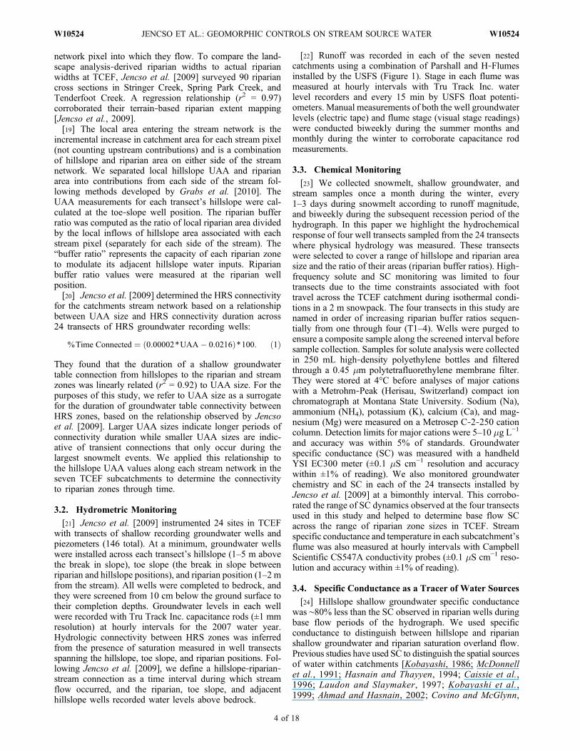
4.1. Precipitation Dynamics[31] We present snow accumulation and melt data from

the Upper Tenderfoot Creek (relatively flat 0° aspect, ele-vation 2259 m) SNOTEL site and rain data from the StringerCreek tipping bucket rain gauge as a reference for HRSgroundwater and runoff response timing in response toprecipitation dynamics (Figure 2). The maximum snow packsnow water equivalent before melt was 358 mm. Springtimewarming lead to an isothermal snowpack, and most of thesnowpack melted between 27 April 2007 to 19 May 2007.Average daily snow water equivalent losses were 15 mmand reached a maximum of 35 mm on 13 May 2007. A finalspring snowfall and subsequent melt occurred between24 May 2007 and 1 June 2007, yielding 97 mm of water.

Figure 2. Water year 2007 cumulative snow water equiv-alent, snowmelt, and rain.

JENCSO ET AL.: GEOMORPHIC CONTROLS ON STREAM SOURCE WATER W10524W10524

6 of 18

Four days following the end of snowmelt, two low!intensityrain storms (totaling 30 and 22 mm, respectively) occurred.

4.2. Hillslope and Riparian Hydrologic Connectivityand Specific Conductance Dynamics[32] We present a detailed description of each transect’s

landscape attributes and resulting HRS connectivity and SCdynamics in Appendix A. Figure 3 depicts each transectsHRS water table connectivity, specific conductance dynamics,

and runoff and SC observed at the LTC catchment outlet.Hillslope to riparian water table connectivity ranged from 9to 123 days across the four transects during the studyobservation period (1 April 2007 to 1 August 2007; Table 1).Hillslope groundwater was characterized by low specificconductance (!27 mS cm"1, ±6.5 mS cm"1, n = 88). Attransects with transient hillslope water tables, ripariangroundwater SC was higher during base flow conditions(!127 ± 36 mS cm"1, n = 72) but shifted by varying degreestoward hillslope signatures following HRS connectivityduring snowmelt (Figure 3).

4.3. Quantifying the Capacity of the Riparian Zoneto “Buffer” Hillslope Connections[33] When hillslope water tables were present, their SC

was consistent and dilute relative to riparian groundwater(Figure 3). Riparian groundwater before spring melt pro-vided a background SC and its change through snowmeltprovided an indication of hillslope/riparian mixing, rates ofriparian water turnover, and riparian buffering. We applied aCSTR mixing model to each riparian SC time series toquantify the rate of decreasing riparian SC in response tohillslope water table development and HRS connectivity.[34] During snowmelt, HRS water table connectivity

developed across each transect that indirectly led to a sig-nificant decrease in riparian SC as more dilute hillslopewater entered and mixed with resident riparian water. Eachtransect exhibited a different turnover rate of riparian water(Figure 4) and goodness of fit to the relationship between ln(SC) and time (r2 ranging from 0.62 to 0.96). T4, the transect

Figure 3. (a–d) Time series of riparian and hillslope watertable dynamics and specific conductance at transects 1–4.Times of hillslope!riparian!stream hydrologic connectivityare indicated with gray shading. Runoff (dark gray shading)and specific conductance (black line) dynamics at the LowerTenderfoot Creek flume are shown (e) for comparison to thetransect dynamics.

Figure 4. Exponential decline of riparian groundwaterspecific conductance toward the hillslope signature follow-ing the snowmelt induced HRS hydrologic connection.The slopes of these lines indicate the rate of riparian waterturnover or dilution by hillslope water. The inverse of theslope is the turnover time constant for each site (Table 1)and provides a measure of riparian buffering of hillslopethroughflow. The dotted line represents the exponentialdecline of LTC stream specific conductance during the sametime period.

JENCSO ET AL.: GEOMORPHIC CONTROLS ON STREAM SOURCE WATER W10524W10524

7 of 18

with the lowest frequency of HRS connectivity and a largeriparian zone turned over at the slowest rate. In contrast,T1 had a continuous connection throughout snowmelt andthe fastest riparian turnover rate. The two intermediarytransects (T2 and T3) exhibited sustained HRS connec-tivity. T2s riparian SC decreased more rapidly from thetime of its initial HRS connection relative to T3. T3 had amuch larger riparian zone (1148 m2) compared to T2 (163m2), and its riparian zone was connected to the hillslopefor a shorter duration (Table 1).[35] We plotted the time it took for each riparian zone’s

SC to decrease to half of its initial value (t50, equation (3))against its riparian buffer ratio (riparian area/hillslope area)to determine the potential of each riparian zone to modulateits corresponding hillslope water table connection. Wefound a logarithmic relationship between the buffer ratioand the t50 time (r2 = 0.95) at each transect (Figure 5;equation (14)):

t50 ! 6:13 ln#Riparian buffer ratio$ & 29: #14$

T1 had the lowest buffer ratio, and it took only 3 days forthe riparian SC to be reduced by half by hillslope inputs.During its continuous HRS connectivity throughout thestudy period (123 days), approximately 27 riparian volumeswere turned over (equation (5); Table 1). T2 had a smallriparian area relative to its hillslope connection duration andthe second shortest turnover half!life (6 days). Six riparianvolumes were exchanged in T2 during its 46 day HRSconnectivity time period. The turnover half!life for T3 was20 days, and !1 riparian volume of mixed hillslope andriparian water was removed during its 29 day HRS con-nectivity time period. T4 had the longest observed turnoverhalf!life (27 days) associated with its large riparian buffer-

ing ratio. Only 26% of the original riparian volume wasturned over during its 9 day HRS connectivity duration.[36] One or more (up to 27) riparian volumes passed

through the transects (T1 and T2) with low riparian bufferingratios and sustained HRS connections resulting in a pre-dominantly hillslope water SC signature in these riparianzones. The two transects (T3 and T4) with larger buffer ratiosnever approached hillslope SC during their HRS connectivityduration. We calculated the time it would take to deplete theoriginal riparian SC at each transect (equation (4)) to evaluatethe effect of changing HRS connectivity duration on thedegree of turnover that can occur at each transect.[37] Figure 6 illustrates the time required; incorporating

each transect’s time constant, for the initial riparian water tobe mixed or replaced by dilute hillslope inflows. T4 wouldrequire 115 days to completely turn over its riparian water,but it was only connected for a total of 9 days duringsnowmelt. T3 would require 86 days to turn over but wasonly connected 29 days. T2 would require 25 days, whichwas less than its observed 46 day HRS connection duration.This was consistent with the observed riparian SC timeseries (Figure 3b) that indicated that riparian SC decreasedto the hillslope groundwater SC over the course of springrunoff. Similarly, T1’s riparian zone only required 13 daysto fully turn over, and its SC dynamics followed those of thehillslope throughout its continuous connectivity duration.

4.4. Comparing Internal Distributions of RiparianBuffering and Turnover to Source Water Separationsat the Catchment Outlet[38] Plot scale hydrochemical time series indicated that

the size of a riparian zone relative to duration of ground-water connectivity to its uplands (as represented by UAAsize [Jencso et al., 2009]) may be a predictor of the turnoverrate of riparian water (equation (14); Figure 5). Riparian and

Figure 5. Logarithmic relationship between the riparianbuffering ratio (riparian area divided by hillslope area) ateach transect and the time that it takes for 50% of the initialriparian concentration to be turned over or diluted by hill-slope water (Table 1; equation (2)).

Figure 6. Estimated hillslope!riparian!stream connectivityduration required for 95% of the initial riparian water to bereplaced or diluted by hillslope throughflow (shaded bars)and the observed HRS connectivity duration for the studyobservation period (white rectangles). The riparian zone isestimated to be turned over when SC reaches hillslope sig-natures (white shading) denoted in each shaded bar.

JENCSO ET AL.: GEOMORPHIC CONTROLS ON STREAM SOURCE WATER W10524W10524

8 of 18

hillslope area typically are not distributed homogenouslyalong stream networks. Different distributions and combi-nations of each can be found in neighboring catchmentsaccording to their landscape structure [McGlynn and Seibert,2003]. We examined how HRS connectivity durations(function of UAA), riparian buffering, and riparian ground-water turnover were distributed within each subcatchmentin TCEF (Figure 7).[39] Figure 7a illustrates connectivity duration curves

(CDCs) [Jencso et al., 2009] for each stream network. EachCDC was derived from the combined 10 m left and rightstream bank frequencies of HRS connectivity for the 2007water year (equation (1)). Catchments with less topographiccomplexity and a higher proportion of larger UAA sizesexhibited elevated annual HRS connectivity and a highermagnitude peak connectivity. Decreased annual connectiv-ity and lower magnitude peak connectivity was character-istic of catchments with more convergence and divergencein the landscape and a higher frequency of small UAA sizes.[40] How riparian areas were arranged next to their

adjacent hillslopes determined the distribution of streamnetwork riparian buffering (Figure 7b) and the resultantturnover times (equation (14); Figure 7c). Catchments with ahigher frequency of larger UAA relative to riparian extentshad less stream network riparian buffering and a higherfrequency of fast riparian groundwater turnover times (andvice versa).[41] We compared the distribution of riparian buffering

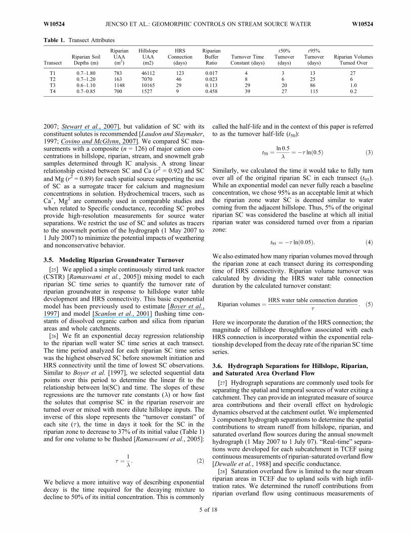
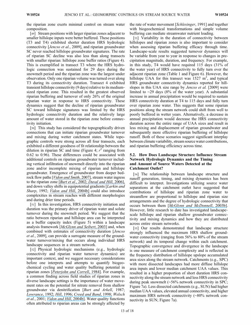
and turnover with the timing and total amounts of ripariangroundwater in each subcatchment’s annual snowmelthydrograph (Table 2). To elucidate potential differences ofsource water contributions across catchments, we determinedthe percentage of riparian, hillslope, and riparian overlandflow contributions to the snowmelt hydrograph before snow-melt (1 April), and during the rising (1 May), peak (14 May),and recession (1 July) of the hydrograph. Figure 8 depictsriparian buffering maps, estimated turnover along the streamnetwork, and snowmelt hydrograph separations for SPC,LSC, and SUN catchments. These catchments span the rangeof turnover distributions and resultant riparian groundwatercontributions found across all seven nested catchments withinTCEF (Figure 9).[42] SPC was characteristic of catchments with a high

degree of riparian buffering (Figures 7b and 8a) and longduration riparian turnover times (Figures 7c and 8d). Asignificant amount of riparian area and buffering potential isaccumulated along the two headwater tributaries of SPC andits mainstem (Figure 8a). This resulted in a high proportionof long duration turnover times along the stream network(Figure 8d) and a median catchment riparian turnover half!life of 15.3 days (Table 2 and Figure 7c). SPC also had thelargest riparian groundwater contribution in its annualsnowmelt hydrograph (Table 2 and Figure 9, SPC). Totalriparian runoff was 97.4 mm for the entire study period.Riparian groundwater contributions were persistent beforesnowmelt (61%) and during the rising (26%), peak (30%),and falling limb (53%) of the annual snowmelt hydrograph(Figure 8g).[43] LSC was more characteristic of other TCEF catch-

ments (UTC, LTC, and MSF) with more moderate values ofriparian buffering (Figure 8b) and turnover half!life valuesalong their stream length (Figure 7c UTC, LTC, MSC, andLSC, and Figure 8e). Within these catchments, the majority

Figure 7. TCEF subcatchment distributions of stream net-work (a) HRS connectivity, (b) riparian buffering, and theresultant (c) riparian groundwater turnover times. Riparianwater turnover times (riparian buffering) are a function ofhydrologic connectivity and the size of the riparian area rel-ative to the adjacent hillslope. Catchments with fast turnovertimes had more sustained HRS connectivity and less riparianbuffering of hillslope inputs. Catchments with longer dura-tion turnover times had shorter duration hillslope ground-water table connectivity to their riparian zones and moreeffective riparian buffering along the stream network.

JENCSO ET AL.: GEOMORPHIC CONTROLS ON STREAM SOURCE WATER W10524W10524

9 of 18

Table 2. Tenderfoot Creek Experimental Forest Catchment Landscape Distributions and Riparian Turnover and Runoff

Catchment% Riparian

AreaMedian Hillslope

UAA (m2)Median Riparian

UAA (m2)Median Buffer

RatioMedian t50time (days)

Total RiparianRunoff (mm)

Riparian Runoff(%)

SPC 6.10 1695 148 0.1330 15.3 97.4 36UTC 4.99 3510 167 0.0640 12.98 34.8 17LSC 3.0 2357 148 0.0591 12.5 45.0 14LTC 3.90 2403 145 0.0597 12.6 39.7 12MSC 3.10 2983 181 0.0578 12.45 37.9 11.3SUN 1.70 4488 156 0.0419 9.8 4.8 1.9BUB 0.89 3345 124 0.0348 9.3 3.2 1.3

Figure 8. Subcatchment (a–c) hillslope UAA, riparian area, and riparian buffering potential (black andred bars), (d–f) the HRS stream network turnover distribution derived from the riparian buffering!turn-over relationship (equation (5)), and (g–i) spatial source water separations for each subcatchment.Catchments with higher riparian buffering and turnover time distributions have a more sustained ripariangroundwater contribution to their annual snowmelt hydrographs.

JENCSO ET AL.: GEOMORPHIC CONTROLS ON STREAM SOURCE WATER W10524W10524

10 of 18

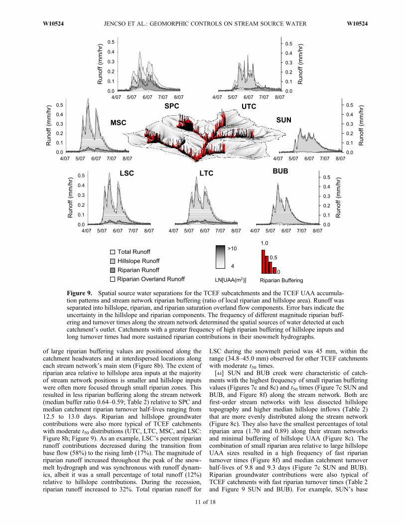
of large riparian buffering values are positioned along thecatchment headwaters and at interdispersed locations alongeach stream network’s main stem (Figure 8b). The extent ofriparian area relative to hillslope area inputs at the majorityof stream network positions is smaller and hillslope inputswere often more focused through small riparian zones. Thisresulted in less riparian buffering along the stream network(median buffer ratio 0.64–0.59; Table 2) relative to SPC andmedian catchment riparian turnover half!lives ranging from12.5 to 13.0 days. Riparian and hillslope groundwatercontributions were also more typical of TCEF catchmentswith moderate t50 distributions (UTC, LTC, MSC, and LSC:Figure 8h; Figure 9). As an example, LSC’s percent riparianrunoff contributions decreased during the transition frombase flow (58%) to the rising limb (17%). The magnitude ofriparian runoff increased throughout the peak of the snow-melt hydrograph and was synchronous with runoff dynam-ics, albeit it was a small percentage of total runoff (12%)relative to hillslope contributions. During the recession,riparian runoff increased to 32%. Total riparian runoff for

LSC during the snowmelt period was 45 mm, within therange (34.8–45.0 mm) observed for other TCEF catchmentswith moderate t50 times.[44] SUN and BUB creek were characteristic of catch-

ments with the highest frequency of small riparian bufferingvalues (Figures 7c and 8c) and t50 times (Figure 7c SUN andBUB, and Figure 8f) along the stream network. Both arefirst!order stream networks with less dissected hillslopetopography and higher median hillslope inflows (Table 2)that are more evenly distributed along the stream network(Figure 8c). They also have the smallest percentages of totalriparian area (1.70 and 0.89) along their stream networksand minimal buffering of hillslope UAA (Figure 8c). Thecombination of small riparian area relative to large hillslopeUAA sizes resulted in a high frequency of fast riparianturnover times (Figure 8f) and median catchment turnoverhalf!lives of 9.8 and 9.3 days (Figure 7c SUN and BUB).Riparian groundwater contributions were also typical ofTCEF catchments with fast riparian turnover times (Table 2and Figure 9 SUN and BUB). For example, SUN’s base

Figure 9. Spatial source water separations for the TCEF subcatchments and the TCEF UAA accumula-tion patterns and stream network riparian buffering (ratio of local riparian and hillslope area). Runoff wasseparated into hillslope, riparian, and riparian saturation overland flow components. Error bars indicate theuncertainty in the hillslope and riparian components. The frequency of different magnitude riparian buff-ering and turnover times along the stream network determined the spatial sources of water detected at eachcatchment’s outlet. Catchments with a greater frequency of high riparian buffering of hillslope inputs andlong turnover times had more sustained riparian contributions in their snowmelt hydrographs.

JENCSO ET AL.: GEOMORPHIC CONTROLS ON STREAM SOURCE WATER W10524W10524

11 of 18

flow riparian contributions initially comprised 67% of run-off. Riparian contributions initially increased during therising limb but decreased to only 1% during peak runoff(Figure 8i; Figure 9 SUN and BUB). During the recession,riparian contributions progressively increased to 17% oftotal runoff. Total riparian runoff for SUN was small(4.8 mm) relative to the majority of the other TCEF catch-ments. BUB was the other TCEF catchment with a similarmedian turnover time (9.3 days), and it exhibited similarriparian runoff dynamics (Figure 9 BUB and Table 2) andtotal contributions (3.8 mm).[45] We compared the percentage of each catchment’s

total riparian area to its total riparian runoff contributionsduring the snowmelt hydrograph (Figure 10). A strong lin-ear relationship (r2 = 0.90) suggested that increasing totalcatchment riparian area can result in increased ripariangroundwater contributions. While this relationship wasstrong, it provides little insight into the relationship betweenthe internal interactions and connections that can occurbetween hillslope and riparian settings within a catchment.[46] We also plotted the median value of each catchments

t50 time (equation (2); Figure 7) against its ripariangroundwater contribution (Figure 9) to better elucidate howthe distribution of water table connectivity (as representedby hillslope UAA size [Jencso et al., 2009]) among localhillslope and riparian area assemblages can affect wholewatershed response (Figure 11). The amount of riparianrunoff exiting each catchment increased linearly withincreasing catchment median t50 time duration (Figure 11;r2 = 0.91).

5. Discussion

5.1. What is the Effect of HRS Connectivity Durationon the Degree of Turnover of Water and Solutesin Riparian Zones?[47] Transient hillslope groundwater tables are important

to the timing and magnitude of runoff and delivery of

solutes to stream networks. Equally important is the potentialfor the riparian zone to buffer hillslope groundwater inputsand thereby stream water composition. We investigatedshallow groundwater hydrologic and specific conductance(as a surrogate of solute concentrations) dynamics acrossfour hillslope!riparian!stream (HRS) transects with differentriparian and hillslope sizes to ascertain controls on riparianbuffering of hillslope runoff and the resulting expression ofhillslope solute signatures in stream water. Our results indi-cate that the intersection of HRS connectivity (as controlledby hillslope UAA size [Jencso et al., 2009]) with riparianarea extents is a first!order control on the degree of riparianwater turnover during snowmelt.[48] Stream positions with riparian zones adjacent to

larger hillslope UAA were poorly buffered. These positionshad longer duration hillslope!riparian!stream hydrologicconnectivity (T1 and T2) and riparian groundwater SC thatmaintained or approached hillslope SC signatures over thecourse of spring runoff (Figure 4, T1 and T2). This indicatedthat riparian water in the riparian zone before snowmelt wasfully mixed and displaced by hillslope groundwater withconnectivity initiation and maintenance. For example, T1,the HRS sequence with the largest hillslope UAA size andcontinuous HRS hydrologic connectivity, had the fastestturnover time (3 days) across the four transects underobservation. The riparian zone of T1 was relatively largecompared to other transects with longer turnover times.However, riparian groundwater SC was always similar tohillslope groundwater SC (Figure 3a). This suggests that thecontinuous delivery of hillslope water to the riparian zoneminimized its buffering potential. Along HRS sequenceswith large hillslope UAA relative to riparian area extents,

Figure 10. The riparian percentage of total runoff duringthe snowmelt period plotted against the percentage of ripar-ian area for each TCEF catchment.

Figure 11. The percentage of riparian runoff during thesnowmelt period plotted against the median of the riparianturnover half life distribution for each TCEF subcatchment.The total riparian runoff observed at each catchment outletwas a function of the distribution of riparian turnover timeswithin each catchment.

JENCSO ET AL.: GEOMORPHIC CONTROLS ON STREAM SOURCE WATER W10524W10524

12 of 18

the riparian zone exerts minimal control on stream watercomposition.[49] Stream positions with larger riparian zones adjacent to

smaller hillslope inputs were better buffered. These positions(T3 and T4) exhibited shorter duration HRS hydrologicconnectivity [Jencso et al., 2009], and riparian groundwaterSC never reached hillslope groundwater signatures. The rateof riparian SC decline was also less than along transectswith smaller riparian: hillslope zone buffer ratios (Figure 4).This is exemplified in transect T3 where the HRS hydro-logic connection was sustained for 29 days during thesnowmelt period and the riparian zone was the largest underobservation. Only one riparian volume was turned over alongT3 during its connectivity duration. Transect 4 exhibitedtransient hillslope connectivity (9 days) relative to its medium!sized riparian zone. This resulted in the greatest observedriparian buffering and turnover of only 26% of the originalriparian water in response to HRS connectivity. Thesedynamics suggest that the decline of riparian groundwaterSC toward hillslope signatures was limited by the HRShydrologic connectivity duration and the relatively largeamount of water stored in the riparian zone before connec-tivity initiation.[50] This study has considered the topographically driven

connections that can initiate riparian groundwater turnoverand mixing during wetter catchment states. While topo-graphic controls were strong across all four transects, eachexhibited a different goodness of fit relationship between thedilution in riparian SC and time (Figure 4; r2 ranging from0.62 to 0.96). These differences could be associated withadditional controls on riparian groundwater turnover includ-ing vertical infiltration of snowmelt directly into the riparianzone and/or incomplete mixing of riparian and hillslopegroundwater. Emergence of groundwater from deeper bed-rock flow paths [Vidon and Smith, 2007], stream water ingressto the riparian zone [Burt et al., 2002; Duval and Hill, 2006],and down valley shifts in equipotential gradients [Larkin andSharp, 1992; Vidon and Hill, 2004b] could also introducecomplexities in stream reaches with different morphologiesand during drier time periods.[51] In this investigation, HRS connectivity initiation and

duration was the primary driver of riparian water and soluteturnover during the snowmelt period. We suggest that theratio between riparian and hillslope area can be interpretedas a buffer capacity index (Figure 5) within a landscapeanalysis framework [McGlynn and Seibert, 2003] and, whencombined with estimates of connectivity duration [Jencsoet al., 2009], can provide a surrogate measure of the ground-water turnover/mixing that occurs along individual HRSlandscape sequences in a stream network.[52] Physical hydrologic mechanisms (e.g., hydrologic

connectivity and riparian water turnover dynamics) areimportant context, and we suggest necessary considerationsbefore one interprets and attempts to quantify biogeo-chemical cycling and water quality buffering potential inriparian zones [Peterjohn and Correll, 1984]. For example,a common finding across field studies of riparian zones indiverse landscape settings is the importance of water move-ment rates on the potential for nitrate removal from shallowgroundwater via denitrification [Burt and Arkell, 1987;Lowrance, 1992; Hill, 1996; Creed and Band, 1998; Welschet al., 2001; Vidon and Hill, 2004b]. Water quality functionsoften attributed to riparian areas can be strongly affected by

the rate of water movement [Schlesinger, 1991] and togetherwith biogeochemical transformations and simple volumebuffering can mediate streamwater nutrient loading.[53] Variability in the duration of connectivity between

hillslopes and riparian zones is also important to considerwhen assessing riparian buffering efficacy through time.Landscape!scale results suggested turnover dynamics willbe variable from year to year in response to changes in pre-cipitation magnitude, duration, and frequency. For example,in this study, T4 would have required 115 days (31% ofthe water year) of HRS connectivity to fully turn over theadjacent riparian zone (Table 1 and Figure 6). However, thehillslope UAA for this transect was 1527 m2, and typicalHRS groundwater connectivity dynamics reported for hill-slopes in this UAA size range by Jencso et al. [2009] werelimited to !29 days (8% of the water year). A substantialincrease in annual precipitation would be required to sustainHRS connectivity duration at T4 to 115 days and fully turnover riparian zone water. This suggests that some riparianpositions along the stream network could shift from well topoorly buffered in wetter years. Alternatively, a decrease inannual precipitation would decrease the HRS connectivityduration across the entire range of UAA sizes and result inless mixing and displacement of riparian groundwater andsubsequently more effective riparian buffering of hillsloperunoff. Both of these scenarios suggest significant interplaybetween climate variability, stream sourcewater contributions,and riparian buffering efficiency across time.

5.2. How Does Landscape Structure Influence StreamNetwork Hydrologic Dynamics and the Timingand Amount of Source Waters Detected at theCatchment Outlet?[54] The relationship between landscape structure and

runoff generation, timing, and mixing dynamics has beendifficult to interpret. Investigations utilizing source waterseparations at the catchment outlet have suggested thatcontributions of hillslope and riparian zone water tostreamflow are proportional to hillslope and riparian sizearrangements and the degree of hydrologic connectivity thatoccurs between them [McGlynn and McDonnell, 2003b].However, little research to date has investigated landscape!scale hillslope and riparian shallow groundwater connec-tivity and mixing dynamics and how they are distributedacross entire stream networks.[55] Our results demonstrated that landscape structure

strongly influenced the maximum HRS shallow ground-water connectivity (ranging from 56% to 80% of the streamnetwork) and its temporal change within each catchment.Topographic convergence and divergence in the landscapeis one measure of catchment complexity and is reflected inthe frequency distribution of hillslope upslope accumulatedarea sizes along the stream network. Catchments (e.g., SPC)with more dissected landscapes had more diffuse hillslopearea inputs and lower median catchment UAA values. Thisresulted in a higher proportion of short duration HRS con-nectivity along the stream network and less HRS connectivityduring peak snowmelt (!56% network connectivity in SPC;Figure 7a). Less dissected catchments (e.g., SUN) had highermedian UAA values, elevated annual connectivity, and highermaximum HRS network connectivity (!80% network con-nectivity in SUN; Figure 7a).

JENCSO ET AL.: GEOMORPHIC CONTROLS ON STREAM SOURCE WATER W10524W10524

13 of 18

[56] The intersection of hillslope area accumulation withits adjacent riparian area indicated riparian buffering poten-tial (equation (14)). We measured an order of magnitudedifference in the median riparian buffering values across theseven subcatchments even though they had similar medianriparian extents (Table 2). This was a result of the spatialorganization of hillslope area accumulation relative to riparianarea extents along the stream network. Catchment topogra-phy and topology resulted in some catchments with morediffuse inputs of hillslope area adjacent to large riparianareas and higher median riparian buffering values (Figures 7band 8a). Lower median riparian buffering occurred in thecatchments with less convergence/divergence that focusedlarger hillslope inputs into smaller riparian zones (Figures 7band 8c).[57] Each catchment’s riparian buffering (Figure 7b) and

riparian turnover (Figure 7c) frequency distributions sug-gested that large differences in the riparian and hillslopegroundwater components would be detected in catchmentrunoff. Catchments with higher riparian buffering wouldhave less riparian groundwater turnover and less expressionof hillslope groundwater in their snowmelt hydrographs.Lower median riparian buffering and faster riparian turnoverwould lead to greater hillslope contributions to streamflowas riparian zones flush in response to more sustained hill-slope connectivity. Independently determined source waterhydrograph separations supported these hypotheses derivedfrom landscape analyses (Figure 11). Total riparian runofffrom each of the seven catchments ranged from 3 to 97 mmduring the seasonal snowmelt period. This is nearly an orderof magnitude difference in riparian groundwater contribu-tions between the seven headwater catchments; all of whichare within 5 km of one another within the greater 22.8 km2

Tenderfoot Creek catchment.[58] Catchment structure also appeared to control the

timing of riparian and hillslope groundwater expressed inrunoff. When HRS connectivity is initiated, water movesfrom hillslopes through riparian zones to the stream result-ing in increased stream flow. However, the hillslope waterfirst mixes with and displaces groundwater stored in theriparian zones before the event (Figure 4). In general, alarger riparian zone results in longer turnover times of thepreconnectivity riparian chemical signature (Figure 5) and amore sustained riparian groundwater contribution to streamflow. Hydrograph separation results from each catchmentindicated an increase in riparian contributions with snow-melt (Figure 11), initiated by HRS connectivity (Figure 3)[Jencso et al., 2009] and mixing and displacement ofriparian water by hillslope water (Figure 4). However, thepersistence of a riparian signature in each hydrograph variedaccording to the timing of turnover across each streamnetwork (e.g., Figures 8d, 8e, and 8f). This suggests that thefrequency of different HRS connectivity durations across thewatershed controls runoff magnitude [Jencso et al., 2009],but it is the intersection of connectivity and the turnoverdynamics of the adjacent riparian reservoirs that controls thesource water signature of the stream (as the mixture ofhillslope and riparian source waters) through time.[59] Our observations suggest that each catchment’s struc-

ture largely controlled the hydrologic and solute dynamicsmeasured in stream flow. Variability in landscape structurecan influence the timing, magnitude, and location of waterdelivery from uplands to near!stream areas during a storm

event. The interaction/intersection of hillslope water andwater stored in the riparian zones determines the timing andproportion of source waters measured at the catchment out-lets. These observations suggest a degree of predictabilitywhen estimating where in the landscape runoff is generatedand its source water composition through time in catchmentsof differing size and structure.

5.3. Landscape Connectivity Conceptual Modelof Runoff Generation, Riparian Buffering,and Source Water Mixing[60] Many field studies have characterized the heteroge-

neity of hydrologic response at the plot, landscape, andcatchment scales. This has resulted in the development ofdetailed and complex characterizations of catchment dynamicsbut little transferability of general principles across catchmentdivides. We suggest hydrologic connectivity as a “mechanismto whittle down unnecessary details and transfer dominantprocess understanding from the hillslope to the catchmentscales [Sivapalan, 2003].” The following paragraphs presenta simple conceptual model of catchment response to snow-melt and precipitation events based on the relationshipsbetween landscape structure, metrics of HRS hydrologicconnectivity, and riparian buffering.[61] Jencso et al. [2009] found that the magnitude of

runoff generation in one watershed at the TCEF was drivenby variability in hillslope UAA size distributions and thefrequency of their lateral connections along the streamnetwork. During base flow periods, the majority of thestream network’s riparian zones were hydrologically dis-connected from their uplands except those adjacent to thelargest hillslopes. As snowmelt proceeded HRS connectivitywas initiated across progressively smaller hillslope UAAsizes and runoff increased with each subsequent connection.Here we suggest that the sequencing of connectivity initia-tion (according to topography and topology) across thestream network determines runoff magnitude through time,but that it is the intersection of connectivity frequency andduration with riparian area extents that controls riparianbuffering and source water components measured at thecatchment outlet.[62] A spectrum of riparian groundwater turnover times is

possible in a given watershed according to the arrangementof hillslope and riparian sizes. HRS sequences with largehillslope UAA (more persistent connections) relative toriparian area will turn over quickly and contribute pre-dominantly hillslope water during the course of an event. Atthe other end of the spectrum, HRS sequences with smallhillslope UAA (transient connections) and larger riparianzones will be well buffered against hillslope throughflowand contribute a more persistent quantity of riparian ground-water to the stream. Therefore, a catchment’s buffering effi-cacy and outlet source water dynamics are a result of anintegration of the frequency and timing of HRS hydrologicconnectivity and associated riparian buffering (turnover)across the stream network. If the riparian buffering potentialexceeds its connectivity duration across the network, then ariparian groundwater contribution will dominate the streamhydrograph. However, greater hillslope connectivity andlower riparian buffering will result in increased turnover ofriparian groundwater and a greater hillslope source watersignature measured at the catchment outlet. Each watershed

JENCSO ET AL.: GEOMORPHIC CONTROLS ON STREAM SOURCE WATER W10524W10524

14 of 18

progresses from the well to poorly buffered case throughtime and with increasing antecedent wetness and event sizeand duration.[63] The value of a conceptual hydrologic model can be

measured by its ability to be effectively transferred toalternate catchments. Contributions of runoff and solutes tothe TCEF stream network are highly variable in time andspace and largely driven by the topographic redistributionof water from the uplands, through riparian zones, and intothe stream network. Many studies have observed strongrelationships between landscape topography and runoffgeneration [Dunne and Black, 1970; Anderson and Burt,1978; Beven, 1978; Burt and Butcher, 1985], runoff spatialsources [Sidle et al., 2000;McGlynn andMcDonnell, 2003b],and water residence times [McGlynn et al., 2004; McGuireet al., 2005; Tetzlaff et al., 2009]. This suggests that metricsof topography, topology, and resulting connectivity couldbe an organizing principle for predicting storm responsein headwater catchments. In other environments, bedrockgeology [Huff et al., 1982; Wolock et al., 1997; Burns et al.,1998; Shaman et al., 2004; Uchida et al., 2005], soil char-acteristics [Buttle et al., 2004; Devito et al., 2005; Soulsbyet al., 2006; Tetzlaff et al., 2009], or other catchment fea-tures could additionally influence and even dominate con-nectivity between source areas and the stream network.[64] Variability in patterns of topography, soils, geology,

and climate all influence runoff generation. However, theircombined effect and relative importance for streamflowdynamics has been difficult to decipher. To attribute appro-priate causal mechanisms to catchment outlet response, weemphasize the importance of internal/distributed hydrologicmonitoring across time. Changing soil moisture states andthe transition from vertical to lateral connectivity in theshallow subsurface [Grayson et al., 1997] or the partitioningof water to/from deeper bedrock storage [Sidle et al., 2000;Shaman et al., 2004; Uchida et al., 2005] can significantlyalter water sources observed in streamflow. For example, arecent distributed assessment of the stream network waterbalance at Tenderfoot Creek indicated that runoff genera-tion transitioned from topographically driven lateral redis-tribution of water and hydrologic connectivity [Jencso et al.,2009] at wetter catchment states to detectable geologic con-trols (!10% stream network connectivity) at low base flow[Payn et al., 2009]. This suggests a potential transition instreamflow generation mechanisms as a function of catch-ment wetness state.[65] Consideration of hydrologic connections and source

areas within the landscape is critical to deconvolution ofcatchment outlet dynamics into their spatial sources andcontrolling mobilization processes. We suggest that the con-ceptualization presented here provides a simple and potentiallyrobust description of runoff response across catchments ofdifferent size and structure and may prove useful for predic-tion in ungauged basins.

5.4. Watershed Management Implications of RiparianBuffering of Landscape Hydrologic Connectivity[66] Riparian zone management to protect and promote

water quality is a valuable strategy across natural and dis-turbed landscapes. However, few tools exist to aid prioriti-zation of riparian management by assessing the relativeimportance of riparian zones across the landscape and their

potential to influence upland runoff and associated waterquality constituents [Allan et al., 2008]. In this paper we havepresented a hydrological context and volumetric bufferingquantification that considers not only riparian zone size andfraction of the total catchment but also an estimate of eachriparian zone’s buffering potential relative to the uplanddelivery of runoff. We focused on the physical hydrologyand tracer behavior across riparian zones. However, thiscontext is also critical for understanding potential for bio-geochemical transformations because it demonstrates theprimary landscape controls on riparian water turnover ratesandmagnitude and provides tools to quantify these processes.For example, water delivery from hillslopes can influence thesupply of oxygenated water to carbon!rich riparian zonesthereby influencing redox state and the potential for micro-bial denitrification [Hill, 2000; Vidon and Hill, 2004a].Better assessment of riparian zone potential to mitigate uplandwater quality degradation, new methods to aide prioritizationof riparianmanagement and protection across space, and toolsto assess catchment!scale riparian buffering potential or con-versely catchment sensitivity to upland loading have strongrelevance to watershed management and applied hydrology!biogeochemistry applications. We suggest that research pre-sented here provides some initial insight not only into howwemight better characterize and quantify riparian zone bufferingpotential at the reach and catchment scales but also highlightthe need for tools to bring these concepts to the riparian andwatershed management communities.

6. Conclusion

[67] Hydrological science continues to search for insightsinto catchment response based on landscape structure. Theresearch described in this paper highlights terrain metricsthat link hydrologic process observations to landscape andcatchment scale response. This approach discretizes thecatchment into its component landscape elements and ana-lyzes their topographic and topologic attributes as surro-gates for their hydrologic connectedness, as measured throughdetailed field observations. On the basis of our high!frequencymonitoring of groundwater connectivity and solute dynamicsfrom the plot to catchment scales we conclude[68] • The degree of riparian water turnover (riparian

buffering) is a function of hydrologic connectivity and thesize of the riparian area relative to the adjacent hillslope.[69] • The frequency of stream network hydrologic con-

nectivity and associated degree of riparian buffering (turn-over) control the timing and magnitude of catchment runoffand solute export.[70] • Catchment structure/organization strongly affects

riparian buffering and runoff source water composition.[71] • Climate variability (wet or dry years) may introduce

a “quantifiable” shift in stream network connectivity and themobilization of water and solutes from riparian and hillslopesource areas.[72] Discretization of catchments into their component

landscape elements and monitoring the hydrochemicalresponse in these landscape elements and by comparingcatchments of varying structure provided insight into thespatial sources of runoff that are hidden by hydrographseparations measured at the catchment outlet alone. Thisapproach allowed us to estimate where runoff and solutemobilization occurred within the landscape and how the

JENCSO ET AL.: GEOMORPHIC CONTROLS ON STREAM SOURCE WATER W10524W10524

15 of 18

integration of these dynamics along the stream network relateto the magnitude of runoff and solute export across catch-ments of differing scale and structure.

Appendix A

[73] We present specific conductance and water tableresults for each transect in order of increasing riparian bufferratios (riparian area/hillslope area) and decreasing hillslopeUAA size and connectivity duration (Figure 3).[74] Transect 1 (T1) was located at the base of a

!20.5° convergent hillslope. It had the largest observedUAA (46,112 m2) of any of the 24 transects, a medium!sized riparian area (783 m2), and the lowest buffer ratio(0.017). The riparian zone exhibited a relatively constantwater table approximately 65 cm below the ground surface(Figure 3a). Groundwater was recorded within 15 cm ofthe ground surface in the hillslope well, located 5 m upslopeof the toe slope break, for the entire water year. Hillslopeand riparian groundwater SC remained relatively constantthroughout the year with a slight dilution during peaksnowmelt (Figure 3a). Riparian groundwater SC dynamicsat this transect always corresponded with those measured atthe hillslope well.[75] Transect 2 (T2) was located along a 7070 m2, !23°

planar hillslope with a small 282 m2 riparian area. Theriparian buffer ratio at this site was 0.039. The riparian watertable remained within 30 cm of the ground surface duringthe year and approached the surface when a hillslope watertable occurred during snowmelt (Figure 3b). The transienthillslope water table first developed on 26 April 2007 andremained connected to the riparian zone through snowmeltuntil 11 June 2007 (46 day HRS connection). Initial ripariangroundwater SC was 108 mS cm"1 and decreased to 29 mScm"1 after a HRS water table connection was established(Figure 3b).[76] Transect 3 (T3) was located near the base of a con-

vergent hillslope hollow (!15.6°) with midrange UAA(10,165 m2) and a large riparian area (1148 m2). Theriparian buffer ratio at this transect was 0.113. Riparian zonewater tables remained within 20 cm of the ground surfacefor the entire year and surface saturation occurred duringsnowmelt and rain events (Figure 3c). A hillslope watertable was first observed on 12 May 2006, exhibiting a rapidrise and sustained connection to its associated riparian zone(Figure 3c). Sustained HRS connectivity was observedduring snowmelt (21 day connection) and the subsequentrain periods (8 day connection), totaling 29 days. Ripariangroundwater before a hillslope water table initiation was185 mS cm"1 but decreased to 77 mS cm"1 after a HRSconnection was established (Figure 3c). Riparian ground-water SC never reached hillslope SC at this transect.[77] Transect 4 (T4) was located along a !26° divergent

hillslope with small UAA (1527 m2) and a large riparianarea (700 m2). The riparian buffer ratio at this site was0.458. The riparian water table remained between 60 and50 cm below the ground surface during base flow butincreased to within 15 cm of the ground surface duringsnowmelt (Figure 3d). The hillslope water table response torain and snow events was highly transient (Figure 3d) andearly in the snowmelt period diurnal HRS water table con-nections/disconnections occurred in association with dailysnowmelt peaks. HRS connectivity was observed for a total

of 9 days at this transect. Riparian SC was 139 mS cm"1

before snowmelt and decreased to 70 mS cm"1 after a hill-slope groundwater table developed (Figure 3d). The ripariangroundwater SC never reached hillslope values at thistransect.

[78] Acknowledgments. This work was made possible by NSF grantEAR!0337650 to McGlynn, EAR!0337781 to Gooseff, and an INRA fel-lowship awarded to Jencso. The authors appreciate extensive logisticcollaboration with the U. S. Department of Agriculture, Forest Service,Rocky Mountain Research Station, especially, Ward McCaughey, Scientist!in!Charge of the Tenderfoot Creek Experimental Forest. We thank JanSiebert, Thomas Grabs, and Robert Payn for technical and collaborativesupport and Galena Ackerman and John Mallard for performing labora-tory analyses. We are grateful to Jennifer Jencso, Vince Pacific, DiegoRiveros!Iregui, and especially Austin Allen for invaluable assistance inthe field.

ReferencesAhmad, S., and S. I. Hasnain (2002), Hydrograph separation by measure-ment of electrical conductivity and discharge for meltwaters in theGanga Headwater basin, Garhwal Himalaya, J. Geol. Soc. India, 59(4),323–329.

Allan, C. J., P. Vidon, and R. Lowrance (2008), Frontiers in riparianzone research in the 21st century, Hydrol. Process., 22, 3221–3222,doi:10.1002/hyp.7086.

Anderson, M. G., and T. P. Burt (1977), Automatic monitoring of soilmoisture conditions in a hillslope spur and hollow, J. Hydrol., 33, 27–36.

Anderson, M. G., and T. P. Burt (1978), The role of topography in con-trolling throughflow generation, Earth Surf. Processes Landforms, 3,331–334.

Beven, K. J. (1978), The hydrological response of headwater and sideslopeareas, Hydrol. Sci. Bull., 23, 419–437.

Boyer, E. W., G. M. Hornberger, K. E. Bencala, and D. M. McKnight(1997), Response characteristics of DOC flushing in an alpine catch-ment, Hydrol. Processes, 11, 1635–1647.

Brinson, M. M. (1993), Changes in the functioning of wetlands along envi-ronmental gradients, Wetlands, 13, 65–74.

Burns, D. A., P. S. Murdoch, G. B. Lawrence, and R. L. Michel (1998),Effect of groundwater springs on NO3

" concentrations during summerin Catskill Mountain streams, Water Resour. Res., 34, 1987–1996,doi:10.1029/98WR01282.

Burns, D. A., J. J. McDonnell, R. P. Hooper, N. E. Peters, J. E. Freer,C. Kendall, and K. Beven (2001), Quantifying contributions to stormrunoff through end!member mixing analysis and hydrologic measure-ments at the Panola Mountain Research Watershed (Georgia, USA),Hydrol. Process., 15, 1903–1924.

Burt, T. P., and B. P. Arkell (1987), Temporal and spatial patterns of nitratelosses from an agricultural catchment, Soil Use Manage., 3, 138–143.

Burt, T. P., and D. Butcher (1985), Topographic controls on soil moisturedistribution, J. Soil Sci., 36, 469–476.

Burt, T. P., L. S. Matchett, K. W. T. Goulding, C. P. Webster, and N. E.Haycock (1999), Denitrification in riparian buffer zones: The role offloodplain hydrology, Hydrol. Process., 13, 1451–1463.

Burt, T. P., et al. (2002), Water table fluctuations in the riparian zone:comparative results from a pan!European experiment, J. Hydrol.,265(1–4), 129–148.

Buttle, J. M., P. J. Dillon, and G. R. Eerkes (2004), Hydrologic coupling ofslopes, riparian zones and streams: An example from the CanadianShield, J. Hydrol., 287, 161–177, doi:10.1016/j.jhydrol.2003.09.022.

Caissie, D., T. L. Pollock, and R. A. Cunjak (1996), Variation in streamwater chemistry and hydrograph separation in a small drainage basin,J. Hydrol., 178, 137–157.

Carlyle, G. C., and A. R. Hill (2001), Groundwater phosphate dynamics ina river riparian zone: effects of hydrologic flow paths, lithology, andredox chemistry, J. Hydrology, 247, 151–168.

Chanat, J., and G. M. Hornberger (2003), Modeling catchment!scalemixing in the near!stream zone: Implications for chemical and isotopichydrograph separation, Geophys. Res. Lett., 30(2), 1091, doi:10.1029/2002GL016265.

Cirmo, C. P., and J. J. McDonnell (1997), Linking the hydrologic andbiochemical controls of nitrogen transport in near!stream zones of tem-perate!forested catchments: A review, J. Hydrol., 199, 88–120.

JENCSO ET AL.: GEOMORPHIC CONTROLS ON STREAM SOURCE WATER W10524W10524

16 of 18

Covino, T. P., and B. L. McGlynn (2007), Stream gains and losses across amountain!to!valley transition: Impacts on watershed hydrology andstream water chemistry, Water Resour. Res., 43, W10431, doi:10.1029/2006WR005544.

Creed, I. F., and L. E. Band (1998), Export of nitrogen from catchmentswithin a temperate forest: Evidence for a unifying mechanism regulatedby variable source area dynamics, Water Resour. Res., 34, 3105–3120,doi:10.1029/98WR01924.

Devito, K., I. Creed, T. Gan, C. Mendoza, R. Petrone, U. Silins, andB. Smerdon (2005), A framework for broad!scale classification of hydro-logic response units on the Boreal Plain: Is topography the last thing toconsider?, Hydrol. Process., 19, 1705–1714, doi:10.1002/hyp.5881.

Dewalle, D. R., B. R. Swistock, and W. E. Sharpe (1988), 3!componenttracer model for stormflow on a small Appalachian forested catchement,J. Hydrol., 104, 301–310.

Dunne, T., and R. D. Black (1970), Partial area contributions to stormrunoff in a small New England watershed, Water Resour. Res., 6,1296–1311, doi:10.1029/WR006i005p01296.

Duval, T. P., and A. R. Hill (2006), Influence of stream bank seepage dur-ing low!flow conditions on riparian zone hydrology,Water Resour. Res.,42, W10425, doi:10.1029/2006WR004861.

Farnes, P. E., R. C. Shearer, W. W. McCaughey, and K. J. Hansen (1995),Comparisons of Hydrology, Geology, and Physical CharacteristicsBetween Tenderfoot Creek Experimental Forest (East Side) Montana,and Coram Experimental Forest (West Side) Montana, Final ReportRJVA!INT!92734, USDA Forest Service, Intermountain ResearchStation, Forestry Sciences Laboratory. Bozeman, Mont., 19 pp.

Genereux, D. (1998), Quantifying uncertainty in tracer!based hydrographseparations, Water Resour. Res., 34, 915–919, doi:10.1029/98WR00010.

Grabs, T., K. J. Jencso, B. L. McGlynn, and J. Seibert (2010), Calculatingterrain indices along streams—A new method for separating stream sides,Water Resour. Res., doi:10.1029/2010WR009296, in press.

Grayson, R. B., A. W. Western, F. H. S. Chiew, and G. Blöschl (1997),Preferred states in spatial soil moisture patterns: Local and nonlocalcontrols, Water Resour. Res., 33, 2897–2908, doi:10.1029/97WR02174.

Hasnain, S. I., and R. J. Thayyen (1994), Hydrograph separation of bulkmeltwaters of Dokriani!Bamak Glacier Basin, based on electrical!conductivity, Curr. Sci., 67, 189–193.

Hill, A. R. (1996), Nitrate removal in stream riparian zones, J. Environ.Qual., 25, 743–755.

Hill, A. R. (2000), Stream chemistry and riparian zones, in Streams andGround Waters, edited by J. Jones and P. J. Mulholland, pp. 83–110,Academic Press, London.

Holdorf, H. D. (1981), Soil Resource Inventory of the Lewis and ClarkNational Forest, Interim. In!Service Report, on file with the Lewis andClark National Forest, Forest Supervisor’s Office, Great Falls, Mont.

Hooper, R., B. Aulenbach, D. Burns, J. J. McDonnell, J. Freer, C. Kendall,and K. Beven (1997), Riparian control of streamwater chemistry: Impli-cations for hydrochemical basin models, IAHS Redbook, 248, 451–458.

Huff, D. D., R. V. Oneill, W. R. Emanuel, J. W. Elwood, and J. D. Newbold(1982), Flow variability and hillslope hydrology, Earth Surf. Proc. Land.,7, 91–94.

Jencso, K. G., B. L. McGlynn, M. N. Gooseff, S. M. Wondzell, K. E.Bencala, and L. A. Marshall (2009), Hydrologic connectivity betweenlandscapes and streams: Transferring reach! and plot!scale understandingto the catchment scale, Water Resour. Res., 45, W04428, doi:10.1029/2008WR007225.

Kobayashi, D. (1986), Separation of a snowmelt hydrograph by specificconductance, J. Hydrol., 84, 157–165.

Kobayashi, D., Y. Ishii, and Y. Kodama (1999), Stream temperature, spe-cific cunductance and runoff process in mountain watersheds, Hydrol.Process., 13, 865–876.

Larkin, R., and J. Sharp (1992), On the relationship between river!basingeomorphology, aquifer hydraulics, and ground!water flow direction inalluvial aquifers, Geol. Soc. Am. Bull., 104, 1608–1620.

Laudon, H., and O. Slaymaker (1997), Hydrograph separation using stableisotopes, silica and electrical conductivity: An alpine example, J. Hydrol.,201, 82–101.

Lowrance, R. (1992), Groundwater nitrate and denitrification in a coastalplain riparian forest, J. Environ. Qual., 21, 401–405.

McDonnell, J. J., M. K. Stewart, and I. F. Owens (1991), Effect ofcatchment!scale subsurface mixing on stream isotopic response, WaterResour. Res., 27, 3065–3073, doi:10.1029/91WR02025.

McGlynn, B. L., J. J. McDonnell, J. B. Shanley, and C. Kendall (1999),Riparian zone flow path dynamics during snowmelt in a small headwatercatchment, J. Hydrol., 222, 75–92.

McGlynn, B. L., and J. J. McDonnell (2003a), Role of discrete landscapeunits in controlling catchment dissolved organic carbon dynamics, WaterResour. Res., 39(4), 1090, doi:10.1029/2002WR001525.

McGlynn, B. L., and J. J. McDonnell (2003b), Quantifying the relativecontributions of riparian and hillslope zones to catchment runoff, WaterResour. Res., 39(11), 1310, doi:10.1029/2003WR002091.

McGlynn, B. L., and J. Seibert (2003), Distributed assessment of contrib-uting area and riparian buffering along stream networks, Water Resour.Res., 39(4), 1082, doi:10.1029/2002WR001521.

McGlynn, B. L., J. J. McDonnell, J. Seibert, and C. Kendall (2004), Scaleeffects on headwater catchment runoff timing, flow sources, andgroundwater!streamflow relations, Water Resour. Res., 40, W07504,doi:10.1029/2003WR002494.

McGuire, K. J., J. J. McDonnell, M. Weiler, C. Kendall, B. L. McGlynn,J. M. Welker, and J. Seibert (2005), The role of topography on catch-ment!scale water residence time, Water Resour. Res., 41, W05002,doi:10.1029/2004WR003657.

Mulholland, P. J. (1992), Regulation of nutrient concentrations in a tem-perate forest streams: Roles of upland, riparian, and instream processes,Limnol. Oceanogr., 37, 1512–1526.

Ocampo, C. J., M. Sivapalan, and C. Oldham (2006), Hydrological connec-tivity of upland!riparian zones in agricultural catchments: Implicationsfor runoff generation and nitrate transport, J. Hydrol., 331, 643–658,doi:10.1016/j.jhydrol.2006.06.010.

Pacific, V. J., K. G. Jencso, and B. L. McGlynn (2010), Variable flushingmechanisms and landscape structure control stream DOC export duringsnowmelt in a set of nested catchments, Biogeochemistry, 99, 193–211,doi:10.1007/s10533-009-9401-1.

Payn, R. A., M. N. Gooseff, B. L. McGlynn, K. E. Bencala, and S. M.Wondzell (2009), Channel water balance and exchange with subsurfaceflow along a mountain headwater stream in Montana, United States,Water Resour. Res., 45, W11427, doi:10.1029/2008WR007644.

Peterjohn, W. T., and D. L. Correll (1984), Nutrient dynamics in an agri-cultural watershed—Observations on the role of a riparian forest, Ecology,65, 1466–1475.

Ramaswami, A., J. B. Milford, and M. J. Small (2005), Integrated Environ-mental Modeling: Pollutant Transport, Fate, and Risk in the Environ-ment, 1st ed., 688 pp., Wiley.

Reynolds, M. (1995), Geology of Tenderfoot Creek Experimental Forest,Little Belt Mountains, Meagher County, Montana, in Hydrologic andGeologic Characteristics of Tenderfoot Creek Experimental Forest, Mon-tana, Final Rep. RJVA!INT!92734, edited by P. Farnes, pp. 21–32,Intermt. Res. Stn., For. Serv., U.S. Dep. of Agric., Bozeman, Mont.

Scanlon, T. M., J. P. Raffensperger, and G. M. Hornberger (2001), Mod-eling transport of dissolved silica in a forested headwater catchment:Implications for defining the hydrochemical response of observedflow pathways, Water Resour. Res., 37, 1071–1082, doi:10.1029/2000WR900278.

Schlesinger, W. H. (1991), Biogeochemistry in freshwater wetlands andlakes, in Biogeochemistry: An analysis of global change, edited byW. H. Schlesinger, pp. 224–260, Academic Press, London.

Seibert, J., and B. L. McGlynn (2007), A new triangular multiple flowdirection algorithm for computing upslope areas from gridded digitalelevation models, Water Resour. Res., 43, W04501, doi:10.1029/2006WR005128.

Shaman, J., M. Stieglitz, and D. Burns (2004), Are big basins just the sumof small catchments?, Hydrol. Processes, 18, 3195–3206, doi:10.1002/hyp.5739.

Sidle, R. C., Y. Tsuboyama, S. Noguchi, I. Hosoda, M. Fujieda, andT. Shimizu (2000), Stormflow generation in steep forested headwaters:A linked hydrogeomorphic paradigm, Hydrol. Processes, 14, 369–385.

Sivapalan, M. (2003), Process complexity at hillslope scale, processsimplicity at the watershed scale: is there a connection?,Hydrol. Process.,17(5), 1037–1041, doi:10.1002/hyp.5109.

Soulsby, C., P. J. Rodgers, J. Petry, D. M. Hannah, I. A. Malcolm, andS. M. Dunn (2004), Using tracers to upscale flow path understandingin mesoscale mountainous catchments: Two examples from Scotland,J. Hydrol., 291, 174–196, doi:10.1016/j.jhydrol.2003.12.042.

Soulsby, C., D. Tetzlaff, P. Rodgers, S. Dunn, and S. Waldron (2006),Runoff processes, stream water residence times and controlling land-scape characteristics in a mesoscale catchment: An initial evaluation,J. Hydrol., 325, 197–221, doi:10.1016/j.jhydrol.2005.10.024.

Stewart, M., J. Cimino, and M. Ross (2007), Calibration of base flowseparation methods with streamflow conductivity, Ground Water, 45,17–27, doi:10.1111/j.1745-6584.2006.00263.x.

JENCSO ET AL.: GEOMORPHIC CONTROLS ON STREAM SOURCE WATER W10524W10524

17 of 18

Tetzlaff, D., J. Seibert, K. J. McGuire, H. Laudon, D. A. Burn, S. M. Dunn,and C. Soulsby (2009), How does landscape structure influence catch-ment transit time across different geomorphic provinces?, Hydrol.Processes, 23, 945–953, doi:10.1002/hyp.7240.

Uchida, T., Y. Asano, Y. Onda, and S. Miyata (2005), Are headwaters justthe sum of hillslopes?, Hydrol. Processes, 19, 3251–3261, doi:10.1002/hyp.6004.

Vidon, P., and A. R. Hill (2004a), Denitrification and patterns of electrondonors and acceptors in eight riparian zones with contrasting hydrogeol-ogy, Biogeochemistry, 71, 259–283.

Vidon, P., and A. Smith (2007), Upland controls on the hydrological func-tioning of riparian zones in glacial till valleys of the midwest, J. Am.Water Resour. Assoc., 43, 1524–1539.

Vidon, P. G. F., and A. R. Hill (2004b), Landscape controls on nitrateremoval in stream riparian zones, Water Resour. Res., 40, W03201,doi:10.1029/2003WR002473.

Welsch, D. L., C. N. Kroll, J. J. McDonnell, and D. A. Burns (2001), Topo-graphic controls on the chemistry of subsurface stormflow, Hydrol. Pro-cesses, 15, 1925–1938.

Weyman, D. R. (1970), Throughflow on hillslopes and its relation to thestream hydrograph, Bull. Int. Assoc. Scientific Hydrol., 15, 25–33.

Wolock, D. M., J. Fan, and G. B. Lawrence (1997), Effects of basin size onlow!flow stream chemistry and subsurface contact time in the NeversinkRiver Watershed, New York, Hydrol. Process., 11, 1273–1286.

K. E. Bencala, U.S. Geological Survey, 345 Middlefield Road, MenloPark, CA 94025, USA.M. N. Gooseff, Civil Environmental Engineering Department, Penn State

University, 212 Sackett Bldg., University Park, PA 16802, USA.K. G. Jencso and B. L. McGlynn, Department of Land Resources and

Environmental Sciences, Montana State University, Bozeman, MT 59717,USA. ([email protected])S. M. Wondzell, U.S. Forest Service, Pacific Northwest Research Station

Olympia Forestry Sciences Lab, Olympia, WA 98512, USA.

JENCSO ET AL.: GEOMORPHIC CONTROLS ON STREAM SOURCE WATER W10524W10524

18 of 18