STATISTICS with applications to HIGHWAY TRAFFIC ANALYSES BRUCE DOUGLAS GREENSHIELDS, C.E., Ph.D. Professor of Civil Engineering The George Washington University FRANK MARK WEIDA, Ph.D. Professor of Statistics The George Washington University THE ENO FOUNDATION FOR HIGHWAY TRAFFIC CONTROL SAUGATUCK . 1952 ' CONNECTICUT

Welcome message from author
This document is posted to help you gain knowledge. Please leave a comment to let me know what you think about it! Share it to your friends and learn new things together.
Transcript

STATISTICSwith applications to
HIGHWAY TRAFFIC ANALYSES
BRUCE DOUGLAS GREENSHIELDS, C.E., Ph.D.Professor of Civil Engineering
The George Washington University
FRANK MARK WEIDA, Ph.D.Professor of Statistics
The George Washington University
THE ENO FOUNDATION FOR HIGHWAY TRAFFIC CONTROL
SAUGATUCK . 1952 ' CONNECTICUT

I
Eno Foundation Publications are provided through an endowment by the late William P. Eno
I
Copyright.I952,bytheEnoFoundationforHighwayTrafficControllnc.Reproductioriofthispublicationinwholeorpartwithoutpermissionisprohibited.Publislied by the Eno Foundation at Saugatuck, Connecticut, October, 1952. Copies of this book are not to be sold.
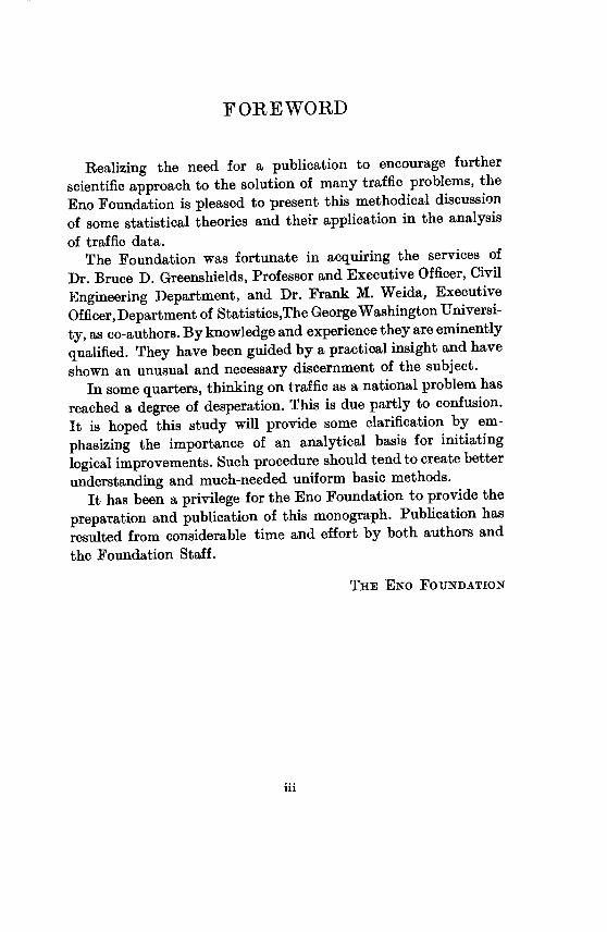
FOREWORD
Realizing the need for a publication to encourage further scientific approach to the solution of many traffic problems, the Eno Foundation is pleased to present this methodical discussion of some statistical theories and their application in the analysis of traffic data.
The Foundation was fortunate in acquiring the services of Dr. Bruce D. Greenshields, Professor and Executive Officer, Civil Engineering Department, and Dr. Frank M. Weida, Executive Officer, Departmentof StatisticsTheGeorgeWashingtonUniversity, as co-authors.Byknowledge and experiencethey are eminently qualified. They have been guided by a practical insight and have shown an unusual and necessary discernment of the subject.
In some quarters, thinking on traffic as a national problem has reached a degree of desperation. This is due partly to confusion. It is hoped this study will provide some clarification by emphasizing the importance of an analytical basis for initiating logical improvements. Such procedure shouldtend to create better understanding and much-needed uniform basic methods.
It has been a privilege for the Eno Foundation to provide the preparation and publication of this monograph. Publication has resulted from considerable time and effort by both authors and the Foundation Staff.
Tiu& ENo FoUNDATION
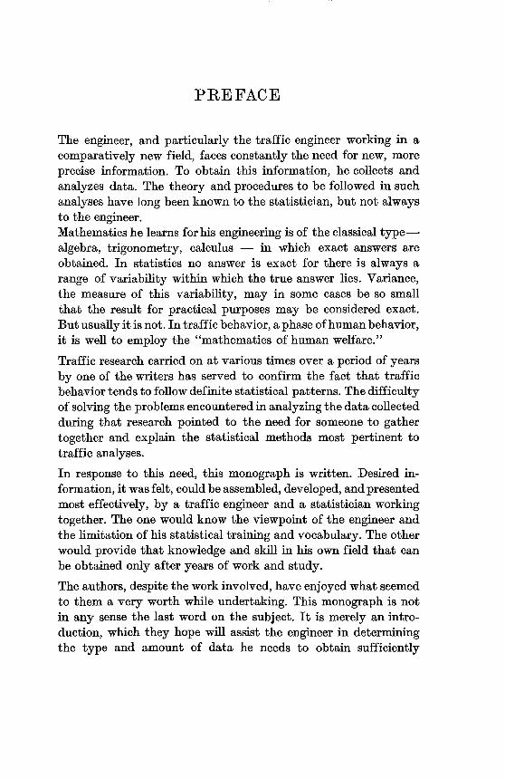
PREFACE
The engineer, and particularly the traffic engineer working in a comparatively new field, faces constantly the need for new, more precise information. To obtain this information, he collects and analyzes data. The theory and procedures to be followed in such analyses have long been known to the statistician, but not always to the enameer. Mathematics he learns forhis engineering is of the classical typealgebra, trigonometry, calculus - in which exact answers are obtained. In statistics no answer is exact for there is always a range of variability within which the true answer lies. Variance, the measure of this variability, may in some cases be so small that the result for practical purposes may be considered exact. But usually it is not. In traffic behavior, a phase of humanbehavior, it is well to employ the "mathematics of human welfare."
Traffic research carried on at various times over a period of years by one of the writers has served to confirm the fact that traffic behavior tendsto follow definitestatistical patterns. The difficulty of solving the problems encounteredin analyzing thedata collected during that research pointed to the need for someone to gather together and explain the statistical methods most pertinent to traffic analyses.
In response to this need, this monograph is written. Desired information, it was felt, could be assembled, developed, and presented most effectively, by a traffic engineer and a statistician working together. The one would know the viewpoint of the engineer and the limitation of his statistical training and vocabulary. The other would provide that knowledge and skill in his own field that can be obtained only after years of work and study.
The authors, despite the work involved, have enjoyed what seemed to them a very worth while undertaking. This monograph is not in any sense the last word on the subject. It is merely an introduction, which they hope will assist the engineer in determining the type and amount of data he needs to obtain sufficiently
vi PREFACE
accurate answers to his problems and save him time and effort. They trust that if it is a new tool to him it will be to his liking.
In the first four chapters the authors have attempted to explain this mathematicaltool, and in the last one they have attempted to show how to use it.
The authors wish to thank the Eno Foundation and staff for its kindly criticism, good counsel, encouragement and sponsorship. They are indebted to Professor Herman Betz of the Department of Mathematics at the Universityof Missouri for his careful review of the manuscript.
WashingtonD. C. BRucE D. GREENSHIELDS
June 1, 1952 FRANK M. WEIDA

ACKNOWLEDGEMENTS
Professor RONALD A. FISHER, Cambridge, Dr. FRANK YATES,
Rothamstead, and Messrs. OLIVER AND BOYD LTD., Edinburgh, for
permissionto reprint Appendix Tables II and IV from their book,
"Statistical Tables forBiological, Agricultural,andXedicalResearch."
GEORGE W. SNEDECOR and the IOWA STATE COLLEGE PRESS, Ames,
Iowa for permission to reprintAppendix Table V from their book
"Statistical Methods," 4th edition.
BUREAU OF PUBLIC ROADS, Washington, D. C. for charts used from
"Highway Capacity Manual."
vii

TABLE OF CONTENTS Page
FOREWORD . . . . . . . . . . . . . . . iii
PREFACE . . . . . . . . . . . . . . . V
AcKNOWLEDGEMENTS . . . . . . . . . . . .Vii
TABLE OF CONTENTS . . . . . . . . . . .ix
LIST OF FIGURES . . . . . . . . . . . . xiv
LIST OF TABLES . . . . . . . . . . . . .XVii
CHAPTER I - THE NATURE AND UTILITY OF STATISTICS
General Remarks . . . . . . . . . . . .Definition and Nature of Statistics . . . . . . .3Statistics and Mathematics
Means of Measuring the Variable and Precautions to be
. . . . . . . . .3Two General Types of Problems . . . . . . .4Types of Sampling . . . . . . . . . . . .5The Variables to be Measured and Interpreted . . .5
Taken . . . . . . . . . . . . . . 6The Size of the Sample . . . . . . . . . .7The Validity and Reliability of Measurement . . . .8Cost of the Project . . . . . . . . . . .9The Report . . . . . . . . . . . . . 9Purpose of the Book . . . . . . . . . . .10References, Chapter I. . . . . . . . . .10
CHAPTER II - SummARiziNG OF DATA . . . . . . .12
Objective . . . . . . . . . . . . . .12Frequency Distribution . . . . . . . . . .12Class Interval and Class Mark . . . . . . . .12Frequency Rectangles . . . . . . . . . .15Histogram . . . . . . . . . . . . . .16Frequency Polygon . . . . . . . . . . .17Smoothed Frequency Polygon . . . . . . . .17
ix
TABLE OF CONTENTS Page,
Frequency Curve . . . . . . . . . . . .18
Mathematical Expectation or Expected Value of a
Moments and Mathematical Expectation of Powers of a
Cumulative Frequencies . . . . . . . . . .19Average . . . . . . . . . . . . . . 22Arithmetic Mean . . . . . . . . . . . .22
Measure of Central Tendency . . . . . . . .27
Variable . . . . . . . . . . . . . .27
Deviation from Arithmetic Mean . . . . . . .27
The Deviations from Any Arbitrary Value . . . .33Mean Values in General . . . . . . . . .33The Mode . . . . . . . . . . . . . . 35Median . . . . . . . . . . . . . . . 38Quantiles . . . . . . . . . . . . . .40
Geometric Mean . . . . . . . . . . . .42
Harmonic Mean . . . . . . . . . . . .44
Root Mean Square . . . . . . . . . . .45
Centra, Harmonic Mean . . . . . . . . . .51Mean or Average Deviation . . . . . . . . .51
Variable . . . . . .. . . . . . . . 54Relation Between Means . . . . . . . . . .58Desirable Properties of an Average . . . . . .58References, Chapter II . . . . . . . . . .60
CHAPTERIII-STANDARDDiSTP.IB-UTIONSAND'fHEIRMATIIE-
MATICAL PATTERNS . . . . . . . . . . . .61
Objective . . . . . . . . . . . . . .61The Elements of a Distribution . . . . . . .61Bernoulli's Theorem . . . . . . . . . . .65Cantelli's Theorem. . . . . . . . . . . .68The Bienaym6-TchebycheffCriterion . . . . . .70
Permutations and Combinations . . . . . . .71Theorem of Compound Probability . . . . . . .74The Binomial Theorem . . . . . . . . . .75
Modal Term of Binomial Distribution . . . . . .79Arithmetic Mean of Binomial Distribution . . . .80

TABLE OF CONTENTS xiPage
Variance of Binomial Distribution . . . . . . 81
Size of Sample Required for Stability . . . . . . 82
The Normal Distribution . . . . . . . . . 85
Interpretation of the Properties of Normal Distribution . 88
Poisson Distribution . . . . . . . . . . . 90
The Sum of the Terms of the Poisson Distribution . . 93
The Arithmetic Mean of Poisson Distribution . . . . 93
The Variance of Poisson Distribution . . . . . . 94
Dispersion and Variance . . . . . . . . . . 97
The Multinomial Distribution . . . . . . . . 102
Hypergeometric Distribution. . . . . . . . . 104
Correlation . . . . . . . . . . . . . . 106
The Correlation Coefficient r-Linear Regression or Linear
Trend . . . . . . . . . . . . . 107Basic Theory of Correlation . . . . . . . . . 113
Coefficient of Regression . . . . . . . . . 115
Standard Deviation of Arrays . . . . . . . . 116
Correlation Ratio: Non-Linear Regression . . . . . 117
Multiple Correlation . . . . . . . . . . . 120Partial Correlation. . . . . . . . . . . . 125
Regression (Trend) Lines . . . . . . . . . . 127
References, Chapter III . . . . . . . . . . 137
CHAPTER IV - SAMPLING THEoRy . . . . . . . . 138
Reliability and Significance . . . . . . . . . 138Objective . . . . . . . . . . . . . . 138
Random Sampling. . . . . . . . . . . . 139
Distribution of Sample Arithmetic Means . . . . . 139
Inference Concerning Population Mean . . . . . 141
Confidence Limits . . . . . . . . . . . . 142
Difference Between Sample Arithmetic Means . . . 143Size of Sample for Arithmetic Mean . . . . . . 145
Reliability of Sample Standard Deviation . . . . . 146
Significanceof Difference Between Sample Variances . . 147
Significance of a Correlation Coefficient . . . . . 147
References, Chapter IV . . . . . . . . . . 149
xii TABLE OF CONTENTS Page
CHAPTER V - SomE APPLICATIONS OF STATISTICAL METHODS 150
Objective . . . . . . . . . . . . . . 150
Test of Goodness of Fit of the Poisson Series to the
Graphical Method of Determining Proportion of Time
Practical Method for Determining Number of Vehicles
Size of Sample to Determine Average Number of Car
Confusion as to Meaning of Highway Capacity . . . 150
Theoretical Maximum Capacity (Volume) . . . . . 151
Stopping Distance and Minimum Spacing . . . . . 152
Interpretation of Minimum Spacing Formula . . . . 154
Limiting Factors . . . . . . . . . . . . 154
Additional Relationships of Spacing and Speed . . . 154
Volume and Speed . . . . . . . . . . . 158
The Nature of the Problems of Highway Traffic . . .160
Spacing as a Random Series . . . . . . . . 161
Test of Goodness of Fit of the Poisson Series . . . . 163
Distribution of Spacings between Vehicles . . . . 163
Minimum Spacing . . . . . . . . . . . . 169
The Minimum Spacing of Four-Lane Traffic . . . . 172
Frequency Distribution of Speeds . . . . . . . 173A Graphical Method of Determining Goodnessof Fit . .178
Estimating Speeds and Volumes. . . . . . . . 181
Estimate of Size Gap Required for Weaving . . . . 187
Physical Features of Highway: Effect on Traffic Flow .187
Crossing Streams of Traffic . . . . . . . . . 189
Mathematical Determinationof Vehicle Delay Time . .190
Occupied by Time-Gaps of Given Size . . . . . 192
The Average Length of All Intervals . . . . . . 194The Signalized Intersection . . . . . . . . . 198
Calculating Delay at Signalized Intersections . . . . 203
Retarded at the Signalized Intersection . . . . . 203
The Average Arrival Method of Determining Delay . . 206
Rare Events (Accidents) . . . . . . . . . . 207
Rare Events (Accidents at Intersections) . . . . . 209
Passengers . . . . . . . . . . . . . 209
Size of Sample Required in Speed Study . . . . . 211
References, Chapter V . . . . . . . . . . 213
TABLE OF CONTENTS Page
APPENDIX
Appendix Table I - Areas under the Normal Probability Curve . . . . . . . 217
Appendix Table II - Table of Values of t, for GivenDegrees of Freedom (n) and atSpecifiedLevelsof Significance (P) 218
Appendix Table III - Ratio of Degrees of Freedom to (t)2 219
Appendix Table IV - Values of Z2 for Given Degrees ofFreedom (n) and for SpecifiedValues of P . . . . . . . 220
Appendix Figure 1 - Values of Z2 for n . . . 221
Appendix Figure 2 - Values of Z2 for n 5, 9, and 17 . 221
Appendix Table V - 5 % and 1 % Points for the Distribution of F . . . . . . . 222
Appendix Table VI - Poisson Table Giving the Probability of x or More Events Happening in a Given Interval, if m,theAverage Number of Events perInterval is Known . . . . . 226
INDEX . . . . . . . . . . . . . . . . 232

LIST OF FIGURES Figure No. Page
11.1 Frequency Rectangles of Observed Vehicle Speeds 1 4
11.2 Histogram of Observed Vehicle Speeds . . . 1 5
11.3 Frequency Polygon of Observed Vehicle Speeds 1 6
IIA Smoothed Frequency Polygon of Observed Vehicle
Speeds . . . . . . . . . . . . . IS
II.5 Frequency Curve of Observed Vehicle Speeds . . 19
II.6 Cumulative Frequency Curve of Observed Vehicle
Speeds . . . . . . . . . . . . . 21
II.7 Arithmetic Mean of Observed Vehicle Speeds 23
11.8 Graphical Representation of the Mean Value 34
11.9 Graphical Solution for Finding the Modal Value of a
Set of Observations . . . . . . . . . 37
11.10 Median Value of Observed Vehicle Speeds . . . 39
II.11 Moment of Inertia of an Area with Respect to a
Parallel Axis . . . . . . . . . . . 46
II. 12 Frequency Diagram . . . . . . . . . . 47
11.13 Mean or Average Deviation of a Set of Observations 52
111.1 Graphical Representation of the PossibleResults of
Tossing a Penny . . . . . . . . . . 76 X2
III.2 Graph of the Equation P(x) = e 2al
89 a 2-7u
mx e7-m 111.3 Graph of the Function P(x) = -- 92
IIIA Illustration of Principle of LEAST SQUARES 108
V.1 Speed in Miles per Hour Corresponding to a Given
Average Density in Vehicles per Mile of Roadway 155
xiv

LIST OF FIGURES xvPigure No. Page
V.2 Average Speed of All Vehicles on Level, Tangent
Sections of 2-Lane Rural Highways . . . . 156
V.3 Average Speed of All Vehicles on Level, Tangent
Sections of the Majority of Existing 2-Lane Main
Rural Highways . . . . . . . . . . 157
VA Speed in Miles per Hour Corresponding to a Given
Volume in Vehicles per Hour on a 2-Lane Highway 159
V.5 Vehicle Time Loss Due to Congestion on a 2-Lane
Highway . . . . . . . . . . . . 160
V.6 Graph Showing Percentage of Vehicle Spacings and
the Probable Amounts of the "Natural Uncertainty"
of the Plotted Points . . . . . . . . . 167
V.7 Distributionof Spacings between Successive Vehicles:
Class Intervals Equal to 5 Seconds . . . . . 169
V.8 Cumulative Frequency Curve of Spacings between
Successive Vehicles . . . . . . . . . 170
V.9 Cumulative Frequency Curve of Spacings between
Successive Vehicles for Various Traffic Volumes on
a Typical 2-Lane Rural Highway . . . . . 171
V.10 Random Distribution of "Influenced" Spacings . . 173
V.11 Cumulative Frequency Curve of Spacings between
Successive Vehicles for Various Traffic Volumes on
a Typical 4-Lane Rural Highway . . . . . 174
V.12 Graph Showing Percentage of Vehicles Traveling
Above and Below Various Speeds and the Probable
Amounts of the "Natural Uncertainty" of the
Plotted Points . . . . . . . . . . 179
V.13 Typical Speed Distributions at Various Traffic
Volumes on Level, Tangent Sections of 2-Lane,
High-Speed Existing Highways . . . . . . 181

xvi LIST OF FIGURES FigureNo. Page
V.14 Frequency Distribution of Travel Speeds of Free
Moving Vehicles on Level, Tangent Sections of the
Majority of Existing 2-Lane Main Rural Highways 182
V. 15 Determination of the Mean Abscissa of the Upper
Half of the Normal Distribution Curve and the
Area to the Right of this Abscissa . . . . . 183
V.16 CumulativeDistributionofTimeSpacesAssumedfor
2-Lane Road Carrying 800 Vehicles per Hour . 184
V. 17 Cumulative Distributionof Time Spaces Assumed for
2-Lane Road Carrying 1200 Vehicles per Hour . 186
V.18 Distribution of Vehicles Between Traffic Lanes on a
4-Lane Highway during Various Hourly Traffic
Volumes . . . . . . . . . . . . 188
V.19 Frequency Distribution of Time Spacing between SuccessiveVehicles Traveling in the Same Direction,
at Various Traffic Volumes on a Typical 4-Lane Rural Highway . . . . . . . . . . 188
V.20 Cumulative Distributionof Time Spaces Assumed for
2-Lane Road Carrying 600 Vehicles per Hour .193
V.21 Probabilities According to Poisson Distribution of
Various Numbers of Vehicles Appearing at an
Intersection During One Signal Cycle . . . . 202
V.22 Additional Blocking Periods Created when Various
Numbers of Vehicles Are Retarded . . . . 205
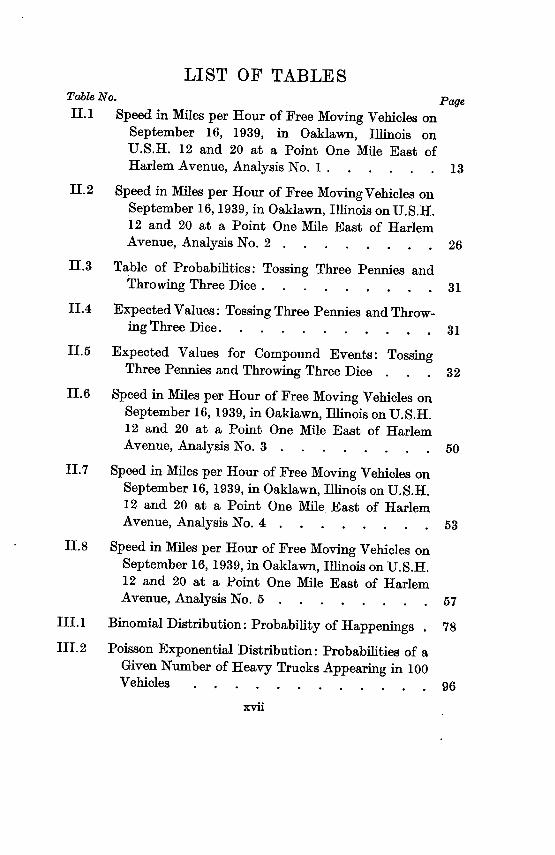
LIST OF TABLES Table No. Page IIJ Speed in Miles per Hour of Free Moving Vehicles on
September 16, 1939, in Oaklawn, Illinois on
U.S.H. 12 and 20 at a Point One Mile East of
Harlem Avenue, Analysis No. I . . . . . . 13
II.2 Speed in Miles per Hour of Free MovingVehicles on September 16,1939, in Oaklawn, Illinois on U.S.H.
12 and 20 at a Point One Mile East of Harlem
Avenue, Analysis No. 2 . . . . . . . . 26
II.3 Table of Probabilities: Tossing Three Pennies and
Throwing Three Dice . . . . . . . . . 31
IIA ExpectedValues: Tossing Three Pennies and Throw
ing Three Dice . . . . . . . . . . . 31
II.5 Expected Values for Compound Events:
Three Pennies and Throwing Three Dice
Tossing
. . . 32
II.6 Speed in Miles per Hour of Free Moving Vehicles on
September 16, 1939, in Oaklawn, Illinois on U. S.H.
12 and 20 at a Point One Mile East of Harlem
Avenue, Analysis No. 3 . . . . . . . . 50
II.7 Speed in Miles per Hour of Free Moving Vehicles on
September 16, 1939, in Oaklawn, Illinois on U.S.H. 12 and 20 at a Point One Mile East of Harlem
Avenue, Analysis No. 4 . . . . . . . . 53
II.8 Speed in Miles per Hour of Free Moving Vehicles on
September 16, 1939, in Oaklawn, Illinois on U. S.H.
12 and 20 at a Point One Mile East of Harlem
Avenue, Analysis No. 5 . . . . . . . . 57
111.1 Binomial Distribution: Probability of Happenings . 78
III.2 Poisson Exponential Distribution: Probabilities of a
Given Number of Heavy Trucks Appearing in 100
Vehicles . . . . . . . . . . . . 96
Xvii

xviii LIST OF TABLES TableNo. Page 111.3 Classification of N = lk IndependentItems in I Rows
of k Items Each . . . . . . . . . . 98
111.4 RelatedValues of Minimum Spacing, Center to Center
in Feet, with Speed in Miles per Hour . . . . 114
II1.5 Simple Correlation of Driver Tests . . . . . 122
III.6 Calculation of Regression (Trend) Functions for the
Data of Table III. 4 . . . . . . . . . 13 2
V.1 Analyses of Reaction-JudgmentDistanceandBrakingDistance for Various Speeds . . . . . . 153
V.2 Fitting of Poisson Curve by Chi-Square Test . . 1 62
V.3 Fitting of Poisson Curve by Individual Terms Table 164
VA Fitting of Poisson Curve by Expected Error Met hod 166
V.5 Calculation of Standard Deviation of Distribution of
Vehicle Speeds . . . . . . . . . . 175
V.6 Fitting of Normal Curve to Distribution of VehicleSpeeds. Chi-Square Method . . . . . . . 176
V.7 Data for Graphical Method of Determining Goodness
of Fit . . . . . . . . . . . . . 179
V.8 Comparison of Theoretical and Field Delays to First
Vehicle in Line . . . . . . . . . . 197
V.9 Comparison of Theoretical and Field Observations of
Total Traffic Delayed . . . . . . . . . 197
V.10 Average Number of Vehicles Stopped with 228
Vehicles per Hour per Lane and 20 Second RedPeriod . . . . . . . . . . . . . 204
V.11 Actual and Expected Distribution of Accidents, In
cluding Casualtiesand Property DamageExceeding
$25, Reported to the CommissionerofMotor Vehic
les of Connecticut, 1931-36, in a Licensed Driver
Sample Selected at Random . . . . . . 207
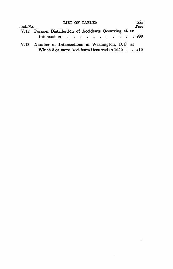
LIST OF TABLES xixTableNo. Page
V. 12 Poisson Distribution of Accidents Occurring at anIntersection . . . . . . . . . . . 209
V. 13 Number of Intersections in Washington, D.C. atWhich 5 or more Accidents Occurred in 1950 . . 210
CIUPTER I
THE NATURE AND UTILITY OF STATISTICS
I. 1. General Remarks. The rapid movement of traffic on our streets
and highways in ever changing patterns is one of the most familiar
andbeneficialphenomenaofour daily lives and atthe sametime one
of the most confusing and vexing. The annoyances and even danger
experienced in driving over congested streets and highways, the
lack of places to park and, in general, the inadequaciesof our high
way system are widely recognized. There is clearly a need for in
creased knowledge of traffic behavior in order that traffic regula
tion and planning may be made more scientific. The method by
which scientific knowledge is increased is to observe what happens
and then by inductive reasoning to establish general laws pertain
ing to these happenings. It is the purpose of this book to develop
a scientific system known as Statistical Methods and show how to
use these methods for analyzing and solving traffic problems.
Mathematical probability, which is the basis of all statistical
theory, had its beginning in ancient times. Certain mathematical
patterns developedas pastimes by the Greeks and others were first
found to coincide with chance happenings such as occur in card
games and later found to coincide with actual happenings. It was
not until the Seventeenth Century that one of the first practical uses was made of probability, when life expectancy tables were
publishedfor use in computing life insurance premiums and bene
fits. Among the early important contributorsto the theory of pro
bability we find the names of DeMoivre, La Place, Gauss, Pascal,
Fermat and Bernoulli. The methods of statistics have long been employed by the
chemist, the sociologist, the physicist, the biologist, the bacteri
ologist, the physiologist, the economist, the meteoroligist, the
business man, the psychologist, and many others. In the biological sciences, the whole theory of evolution and heredity rests in reality
on a statistical basis. Likewise, the behavior of thebodymechanism
itself lends itself to statistical analysis. Statistical theory is the
2 STATISTICS AND HIGHWAY TRAFFIC ANALYSIS
basis of various aspects of theoretical physics and chemistry as de
monstrated by Gibbs, Bohr, Einstein, Fermi, Dirac and others. In
the social sciences, statistics is used in the measurement of the
sizes of the population, the birth, marriage, mortality and morbi
dity rates, and in determiningthe distributionof the population by
trade or income, wages, prices, production, foreign trade, and
transportation. In manufacturing, statistics facilitates efficient
management, economic control of the quality of manufactured
products, and the evaluation of laws of behavior to determine
control or lack of control. Statistics is the basis of corrective legis
lation. But in spite of this wide-spread use, it is only within the
last few years that the traffic engineer has come to realize that
statistics is his most useful tool'- The traffic engineer should fully
realize the importance of the statistical approach to the solution
of his problems. If therehas been some failure on his part to do so,
it no doubt is due to its omission from his engineering training in
which he has been taught to assume that the values with which he
is dealing are exact and always the same. Each individualpiece of
material of a given kind and size is assumed to behave the same as
any other piece of the same kind and size. Statistics deals with
measurements which at best are approximate values which are
usually not the same when repeated. In traffic engineering, the in
dividuals are human and it can not be assumed that they will
always behave in precisely the same manner.
The automobile does not become a complete mechanism until
the driver is behind the wheel. It is the driver who sees the curve
ahead and turns the steering wheel accordingly, who sees the ob
struction and applies the brakes. It is the emotional and physical
characteristicsof the driver that must be measured and evaluated.
To this end, the trafficengineer must use the special type of mathe
matics that applies to the problem he is considering.
In this attempt to make statistics more readily available to the
traffic engineer and others, an effort will be made -not only to ex
plain statistical methods, but to show by example how they may
be used in the solution of trafficproblems. An understanding of the
calculus is desirable but not essential for use of the methods in
volved. In using statistics it must be kept in mind that it is the
3 NATURE AND UTILITY OF STATISTICS
handmaidenof reality and not reality itself. In all cases it must be
demonstratedthat the statisticallaw of behavior to be used agrees
with actual behavior.
As the statistical methods axe developed, it will be found that
they constitute a unified structure. This will become apparent as
the developmentis followed step by step. The first step win be to
explainstatisticalterms through the derivation and explanationof
the mathematical and statistical probabilityformulae which form
the basis of statistics. The use of these formulas win become clear
through their application to the solution of typical problems.
1. 2. Definition and Nature of Statistics. Statistics is the funda
mental and Most important part of inductive logic. It is both an art
and a science, and it deals with the collection, the tabulation, the
analysis and interpretation of quantitative and qualitative mea
surements. It is concerned with the classifying and determining of
actual attributes as well as the making of estimates and the testing
of various hypotheses by which probable, or expected, values are
obtained. It is one of the means of carrying on scientific research
in order to ascertain the laws of behavior of things- be they animate or inanimate. Statistics is the technique of the Scientific Method.
1. 3. Statistics and Mathematics. Statistics is a branch of applied
mathematics. It differsfrom so-calledpure mathematics in thatthe
values in statistics are approximationsor estimates, but -not mere
guesses. The rules and methods of operation are those of pure
mathematics for it is the tool of statistical analysis.
An "exact" value in pure mathematics may be thought of as
one of the possible values a variable may assume. There are but
two possibilities in pure mathematics, namely: the variable has a
certain value or it does not have that value. In the first case, the
probability is 1, meaning that it is certain that the variable has
that value, while in the second case the probability is zero, mean
ing that it is certain that the variable does not have that value. The variable in statistics, called stochastic variable or variate, is
much more general than the variable in pure mathematics. The
stochastic variable is one, to each of the many possible values of

4 STATISTICS AND HIGHWAY TRAFFIC ANALYSIS
which, there is attached a probability, p, that it attains said value. As will be shown in Chapter III, this probability may have any value between zero and one. This fact is expressed mathematically as 0 :< p < 1.
The stochastic or random variable may be discrete or continuous. It is called discrete if it can take on only certain isolated values in an interval and it is called continuous if it can take on any value in an interval. It is to be noted that the probability that a continuous stochastic variable has a specific value is always zero.
J. 4. Two General Types of Problems. Statisticsdeals withproblems that fall into two general categories.
1. The first of these categories of problemshas to do with characterizing a given set of numerical measurements or estimates of some attribute or set of attributes applying to an individual or a given group of individuals. This entails the finding of a mathematical model that fits the pattern of the variation in measurements or the variation in the things being measured. The engineer is familiar with the fact that a distance may be measured several times with a different result each time, and he knows that the mathematicalpatterncalled " The Principleof Least Squares" is used in characterizing such measurements. In studying some attribute such as the ability of students, it is found that there are just a's many brighter than "average" as there are less bright and this pattern is called "normal" and there is a mathematical equation for such a normal curve. Other laws of behavior (distributions) are found to follow other mathematical patterns, such as Poisson's "random" curves (distributions), the Pearson system of distribution and others.
Fortunately, these mathematical patterns are all of the same basic nature. It will be one of our tasks to describe and explain this phase of statisticalmathematics.
2. The second category of problemshas to do withcharacterizing an attribute or attributes belonging to all individuals of the group one is investigating, such as all white pine lumber or all the people living in Ponca City, all people with red hair, or all aluminum alloys of a given specification. These well defined classes of items

5 NATURE AND UTILITY OF STATISTICS
are called populations or "universes". This second class of problems
involves the selection of random samples from the population, the
statistical study of these samples, and the drawing of inferences from them.
The problems just mentioned indicate that (1) the data must be summarized as will be discussed in Chapter II; (2) they must be
thoroughly analyzed by obtaining mathematical patterns of the
laws of their behavior as will be discussed in Chapter III; and (3)
it must be possible to draw inferences from the samples in regard to the reliability and significance of pertinent summary values
obtained from the samples for the purpose of characterizing the "universe" as will be discussedin Chapter IV.
1. 5. Types of Sampling. One may classify random samplingin two
ways: (1) Sampling by attributes; and (2) Sampling by variables,
either discrete or continuous. In samplingby attributes, one deter
mines the number of times (the frequency) the event happenedas
specified and the numberof timestheevent didnothappenasspeci
fied. In samplingby variables, we measuresuch thingsastheweight or length of an object, the duration of an event or the intensityofa
force. We may also measure a group of individuals in order to
characterize them in regard to multiple categories such as weights,
heights, temperatures, etc., to be considered jointly. The basis of
all such characterizations is counting. Hence we must determine
the frequency of the occurrence of a characteristicor event among
n possible occurrences or non-occurrences or among n trials.
1. 6. The Variables to be Measured and Interpreted. The statistical or
scientific method applies not only to the analysis and interpreta
tion of data but to the whole procedure of first recognizing the
need for increased knowledge about a particular problem; second,
the gathering of data aboutthe problem; third, studyingthe significance of the data; and finally, presenting the results of the in
vestigation in a report. In carrying out this statistical procedure there are certain precautions that must be observed.
The recognition of the need for more information about a particular problem usually comes from those who have to deal with it.
6 STATISTICS AND HIGHWAY TRAFFIC ANALYSIS
A researchproject conducted in Ohio in 19394 will serve to illustrate the steps in conducting an investigationto obtain certain specific information. This study had to do with center-line markings of roadways. The fact that different states had, and still have, different systems of markings, causing confusion to motorists, pointed to the obvious need of determiningthe best type.
The first question to be answered was: Is the problem solvable by statisticalmethods ? If so, what method or methods are applicable, what variables need to be measured, how much data are needed, and how best to obtain the needed data?
In the problem of center-line marking, one is interested in the qualities that make a good center-line marking. Some such qualities are visibility, interpretability and durability. But what about other things ? Is a broken line just as satisfactory for a center-line as a solid line? The broken line is cheaper because it requires less paint. What kind of a line or lines should be used to mark a "no-passing" zone? Such questions, of course, can only be answeredafter the study is made. Hence it was necessary to make a provisional conjecture as to what types of center-line marking should be tested.
I. 7. Means of Measuring the Variable, and Precautions to be taken. Having decided provisionally on what types of center-lines to test, the next step was to devise a means of measurement. Should it be done by noting the behavior responsepatternof drivers to different types of markings ? Should a speed check be made ? Should drivers be questioned? Should some other methods be used? What is the probable cost and efficiency of the different possible methods? What type of equipment is necessary to make the recordings ?
It has been found by experience that it is sometimes necessary to design and construct special equipment or apparatus to record field data. It is recaRed that in 19322 it was only after considerable thought that the rather simple expedient of time-motion pictures was used to record the speed and spacing of vehicles. A mechanical device, provided it is first checked for mechanical defects, is always more reliable than human judgment. The picture method possessed one other feature that is not often attained. It
7 NATURE AND UTILITY OF STATISTICS
gave complete informationon all that happenedwithin the field of
view. The pertinent information could then be selected at leisure
and if a wrong conjecture was made, other information already in
hand could be studied.
It was decided in the 1939 project to take speed recordings with
the Eno-scope, a device using mirrors so arranged that the time at
which a vehicle passes two successive positions on the roadway
can be recorded by means of a stopwatch. These positionsmust be
a considerable distance apart, usually 88 or 176 feet, so that the
human variation in snapping the watch will not cause an appreci
able error. Another source of error that is not so readily apparent
is the inability of the observer to take a random sample without
taking the proper precautions to obtain one. It would seem that if
the observer simply recorded the speed of as many vehicles as
possible it would result in an unbiased sample, butsuch is not the
case. Vehicles tend to bunch into queues behind the slower drivers.
Depending upon the alertness of the observer, he may be un
consciously selecting slow or fast vehicles. He must arbitrarily
select some convenient numberedvehicle such as every third one. This device is not infallible. Suppose, for instance, that an
origin-destination survey is being conducted to determine the
travel routes of people living in different sections of a city, and
that it has been decided to interview every tenth house starting
from an arbitrary point. But would we be correct in assumingthat
every tenth house constitutes a good random sample? It could be
that every tenth house is a corner house and hence may be a shop
of some kind. In this case, some special procedure must be used,
such as writing the numbers on cards and after shuffling, picking
every tenth card.
I. S. The Size of the Sample. The size of the sampleis the quantityof
data needed to meet certain considerations. One of the considera
tions is cost, another is time. These depend upon the decision as to (1) the maximum.error that will be tolerated and (2) the degree of
certaintydemanded that this allowable or maximumerror win not
be exceeded. This definitely determines the size of the sample or the
amount of data to be collected. The methodof gathering the data
8 STATISTICS AND HIGHWAY TRAFFIC ANALYSIS '
is largely dependent upon the structure and character of the "universe" from which the sample is taken.
In the Ohio study of 1939, it was desired among other things to get the opinions of drivers about center-lines. Did they prefer a yellow line, a white one, a broken line, or a solid line? The obvious procedure was, of course, to stop each motoristand ask his opinion. But how many? Would the majority of 30 or 40 people agreeingon one combinationas being the best be sufficient ? At first one might possibly say yes, but on second thought he would realize that an opinions might not be unbiased. Perhaps the drivers from Pennsylvania had grown accustomed to a certain combination and would prefer that, or the drivers from Ohio might prefer a different system. This possible tendency to biased opinions meant that a larger sample should be taken and also that along with the opinions, the residence of the driver should be ascertained.
Sometimes opinions are unconsciously biased. This fact also was brought out in the Ohio study. It was decided to try road signs worded to warn drivers that they were entering a "no-passing" zone. It was doubted that a large percentage of the motorists would see the signs, but surprisingly enough, over 98 percent of them stated they had seen the signs. This was so unexpected that it was questionable, and away of checkingthese answerswas sought.
The means of checking was revealed through consideration of the purpose of the sign. Signs aside from thosewhose shapeconveys a message, must be read. A sign much larger than the "no-passing" sign was prominentlydisplayed to warn the drivers thattheywere entering a "test-zone". This might have been guessed from the fact that they had seen 3 or 4 different types of marking within a mile or so, but, over one-third when questionedsaid they did not know they were in a "test-zone". The conclusion reached was that at least one-third and probably more did not see the "no-passing" signs in spite of the fact that 98 percent said they had.
I. 9. The Validity and Reliability ofNeasurement. It is not only opinion measurements that must be checked for validity. In a studyof brake-reaction-time made in Ohio in 19343, it was decided to determine whether the facts warranted the assumption that those

9 NATURE AND UTILITY OF STATISTICS
with quick reaction-time were safer drivers. It was perhaps perfectly logical to assume that a quick reaction will enable a driver to avoid accidents, but the study showed no relationship of accidents to brake-reaction-time.If this were true, and other investigations have shown that it is, then we deduce that an individual with a slow reaction-timeemploys a larger margin of safety and so compensates for his shortcoming. In other words, brake-reactiontime is not a valid measurement to determine whether a driver is a safe driver or not since it does not in fact measure what it was supposed to measure.
A measurementis reliable if there is consistency in obtaining it. In other words, consistency in measurements increases our confidence in the reliability of the conclusion we wish to draw from the set of measurements.
1. IO. Co8t of the Project. After the amount of data needed to obtain results accurate to the degree desired has been estimated, the apparatus needed has been decided and the procedure outlined, it is possible to estimate the minimum cost. This cost will depend to a large extent on the amount of personnel needed and the time required to complete the study. The cost of developmentresearch is easier to estimate than that of basic or fundamental research. In the former we know much more about the expected results. Development research follows the fundamental. It is often used to verify results that have been suggested by more basic studies. In any case, however, it is necessary to estimate the cost. The skill of the researcher is rightly or wrongly measured by his ability to estimate correctly this cost and effort required to carry on an investigationto the point where definite results, whetherpositive or negative, are obtained and reported.
I. II. The Report. A preconceived idea or system of thinking must not be allowed to influence the reporting of results. A negative result is just as important as a positive one. Too often an investigation is conducted to prove a point and this attempt to adhere to an established opinion may have undue influence in selecting the attribute to measure.
10 STATISTICS AND HIGHWAY TRAFFIC ANALYSIS
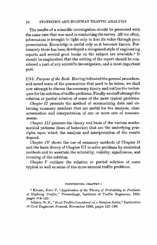
The results of a scientific investigationshouldbe presented with the same care that was used in conductingthesurvey. All too often, information is brought to light only to lose its value through poor presentation. Knowledge is useful only as it becomes known. Fortunately there has been developed a recognized style of engineering reports and several good books on the subject are available.5 It should be emphasized that the writing of the report should be considered a part of any scientificinvestigation, and a most important part.
V 1 2. Purpose of the Book. Having indicated the general procedure, and noted some of the precautions that need to be taken, we shall now attemptto discuss thenecessary theoryand outlinethe techniquesfor the solutionof traffic problems. Finallywe shall attemptthe solution or partial solution of some of the more typical problems.
Chapter II presents the method of summarizing data and obtaining summary numbers that are useful for the analysis, characterization and interpretation of one or more sets of measurements.
Chapter III presents the theory and basis of the various mathematical patterns (laws of behavior) that are the underlying principles upon which the analysis and interpretation of the results depend.
Chapter IV shows the use of summary methods of Chapter II and the basic theory of Chapter III to solve problems by statistical methods and to ascertainthe reliability,validity, significance, and meaning of the solution.
Chapter V outlines the solution or partial solution of some typical as well as some of the more unusual traffic problems.
REFERENCES, CHAWER I
]Kinzer, John P. "Application of the Theory of Probability to Problems of Highway Traffic," Proceedings, Institute of Traffic Engineers, 1934, pages 118-123.
AdamsW.F., "Ro-al TrafficConsidered as'aRandomScries,"Institution of Civil Engineers Journal, November 1936, pages 121-130.

11 NATURE AND UTILITY OF STATISTICS
Greenshields, Bruce D., "Initial Traffic Interference," Presented for discussion at the 16th Annual Meeting of the Highway Research Board, November 19, 193 6, Washington, D. C., 9 pages mimeo and the comments by W. F. Adams
2 Greenshields, Bruce D., "The, Photographic Method of Studying Traffic Behavior," Proceedings, High-way Research Board, Washington, D.C., 1933 pages 384-399.
Ibid., Schapiro, Donald; and Ericksen, Elroy L.; "Traffic Performance at Urban Street Intersections," Yale Bureau of HighwayTraffic, New Haven, Connecticut, 1947, pages 73-118.
,2 Ibid., "Reaction Time in Automobile Driving," Journal of Applied Psychology, Vol. XIX, No. 3, June 1936, pages 353-358.
4 Report of Highway Research Board Project Committee on "Markings for No-Pa8sing Zones," November 1939.
5Nelson, J. Raleigh, "Writing The Technical Report," Me Graw-Hill Book Co., 1947.
CHAPTERII
SUMMARIZING OF DATA
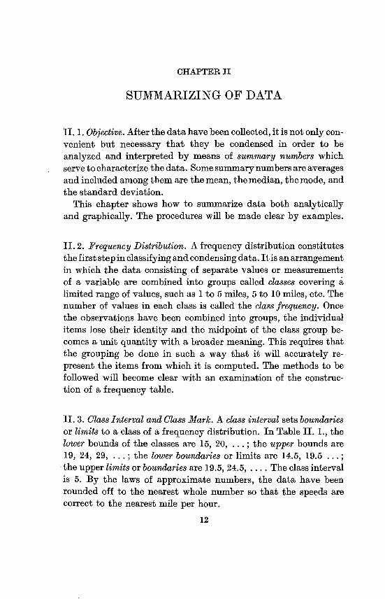
IL 1. Objective. After the datahave been collected, it is not only con
venient but necessary that they be condensed in order to be
analyzed and interpreted by means of summary numbers which
servetocharacterize the data. Somesummarynumbers are averages
and included among them are the mean, the median, themode, and
the standard deviation.
This chapter shows how to summarize data both analytically
and graphically. The procedures will be made clear by examples.
IL 2. Frequency Distribution. A frequency distributionconstitutes
the first step in classifyingand condensingdata. It is an arrangement
in which the data consisting of separate values or measurements
of a variable are combined into groups called classes covering a
limitedrange of values, such as I to 5 miles, 5 to 10 miles, etc. The
number of values in each class is called the class frequency. Once
the observations have been combined into groups, the individual
items lose their identity and the midpoint of the class group be
comes a unit quantity with a broader meaning. This requires that the grouping be done in such a way that it will accurately re
present the items from which it is computed. The methods to be
followed will become clear with an examination of the construc
tion of a frequency table.
11. 3. Class Interval and Class -Mark. A class interval sets boundaries
or limits to a class of a frequency distribution. In Table IL L, the
lower bounds of the classes are 15, 20, . .. ; the upper bounds are
19, 24, 29, . . . ; the lower boundaries or limits are 14.5, 19.5 ... ;
the upper limits or boundaries are 19.5, 24.5, . .. . The class interval
is 5. By the laws of approximate numbers, the data have been
rounded off to the nearest whole number so that the speeds are
correct to the nearest mile per hour.
12

13 SUMMARIZING OF DATA
Table II. I
SPEED IN MILES PIER HOUR OF FREE MOVING VEHICLES ON SEPTEM13ER 16,1939,IN OAKLAMIN, ILLINOIS ON U.S.H. 12 and 20 AT A POINT ONE MILE EAST OF
HARLEM AVENUE
(1) (2) (3) (4) (5) (6) (7)
Speed Number Smoothed PerCent Relative, Cumulative Cumulative in of Fre- of Frequency Frequency PerCent
m.p.h. Vehicles quency Vehicles Frequency
f fe 100 f/n f/n fe 100 fe/n
70-74 0 0 0 0 65-69 0 0.7 0 0 60-64 2 5.7 0.67 0.0067 300 100.00 55-59 15 10.3 5.00 0.0500 298 99.33 50-54 14 19.3 4.67 0.0467 283 94.33 45-49 29 39.0 9.67 0.0967 269 89.67 40-44 74 54.3 24.67 0.2467 240 80.00 35-39 60 65.7 20.00 0.2000 166 55.33 30-34 63 50.7 21.00 0.2100 106 35.33 25-29 29 32.7 9.67 0.0967 43 14.33 20-24 6 14.3 2.00 0.0200 14 4.67 15-19 8 4.7 2.67 0.0267 8 2.67 10-14 0 2.7 0 0 0 .00
300 = n 300.1 = n 100.02 1.0002
Data furnished by Public Roads Administration, Washington, D. C.
Note: This illustrationis of a continuous stochastic variable which may take any value. An illustration of a discontinuous variable is the numbers of vehicles that pass over a highway in any time interval. There is no such thing as a part of a vehicle. An illustrationof a discontinuous stochastic variable where only even integers are possible is the distributionof rows of kernels on ears of corn.
A class mark is the mid-valueof the class interval. In Table II. I.,
column (1), the class marks are 17, 22, 27..... The exact values of a discontinuous variable are usually taken
equal to the class marks. For many purposes, all the values of a
continuous variable that fall within a given class interval are
grouped at the class mark as a convenient approximation.
The number of values that the variable has within a certain class
interval is called a class frequency. In Table II. 1. the frequency 63 in column (2) corresponds to the class 30-34 in column (1).

14 STATISTICS AND HIGHWAY TRAFFIC ANALYSIS
Two conditions which serve as a guide in the choice of the size of
a class interval are: (a) the desire to be able to treat all the values
assigned to any one class, without appreciable error, as if they
were equal to the mid-value or class mark of the class interval:
lb) for convenience and brevity, it is desirable to make the class
interval as large as possible, but always subject to the first con
dition. These two conditions will in general be fulfilled if the inter
val is so chosen that the number of classes lies between ten and
thirty. This does not mean, however, that the minimum may not
be less than ten classes nor the maximummore than thirtyclasses;
f1i
70
60
so
40
30
20
10
L//--0 FTn -n A .1 In In In
0i 0i 0) 14 c7i .4C\J CIJ en M 't In In 10
Speed in Miles Per Hour
FiGuRE 11. I
F1REQUENCY RECTANGLES OF OBSERVED VERICLE SPEEDS

SUMAURIZING OF DATA 15
it merely means that in most cases it is possible to form the classi
fication with the number of intervals lying between ten and
thirty.
Another convenient means of classification is the graphical
summary method. There are five types of graphs that have been
found useful: namely, the Frequency Rectangles, the Histogram,
the Frequency Polygon, the Smoothed Frequency Polygon, and the Frequency Curve. We shall now discuss these in the order named.
f
70
60
50.2
40
30
20
10
0 t IN 'A zk Zs ;A J5
Speed in Miles Per Hour
FiGuRE II. 2
HISTOGRAM OF OBSERVED VEHICLE SPEEDS
11. 4.Frequency Rectangles. Usingthefrequencydistributionas given
by columns (1) and (2) in Table II. 1., the rectangles, shown in

16 STATISTICS AND IIIGHWAY TRAFFIC ANALYSIS
Figure II. I may be drawn. The class intervals are the bases and the altitudes (ordinates) are equal to the frequencies of the classes.
Unit area is defined as that of a rectangle whose base is a class interval and whose altitude is a unit of frequency. This gives a one to one correspondence between area and frequency. In other
f I,
70
60
50
40
E 30
20
10
cm 0 to
Speed in Miles Per Hour
FiGuRE II. 3
FREQUENCY POLYGON OF OBSERVED VEMCLE SPEEDS
words, since the base is equal to one (class interval), the height is thefrequency.
II. 5. Histogram. A histogramis the systemof upper bases ofthe frequency rectangles. It is illustrated in Figure II. 2. for the frequency distributiongiven by columns (1) and (2) of Table II. 1.

17 SUMMARIZING OF DATA
IL 6. Frequency Polygon. A frequency polygon is formed by selec
ting a convenient horizontal scale for the variable being measured
and a vertical scale for the class frequency and then plottingthe
points so that the class marks are the abscissas and the class fre
quencies are the ordinates. This method is shown in Figure IL 3.
for the distribution given in Table IL 1.
IL 7. Smoothed Frequency Polygon. The smoothedfrequencypolygon is a means of graduationsometimescalled a methodofmoving aver
ages. It is useful in obtaining an approximation to the probable
frequency curve or theoretical law of behavior of the attribute that is being measured.
One method of obtaining moving averages is illustrated in
Columns (1), (2), (3), in Table IL L, in which the smoothed value
for an interval is obtained by summing the frequencies in that
interval and the two adjacent intervals and dividing by three.
Hence, the smoothed value for the interval 15-19 is equal to the
sum of the frequencies 0, 8, and 6, divided by 3. For the interval
20-24, we add the frequencies 8, 6, and 29, and divide the sum by
3. We proceed likewise for the remaining intervals. The smoothed
frequency polygon for the distribution given in columns (1) and
(3) of Table 11. 1. is shown in Figure IL 4. By comparing Figure
IL 4 with Figure IL 3., it is seen that the smoothed frequency
polygon has removed the irregularities found in Figure IL 3. and
is closer, in appearance, to a frequency curve. See definition of
frequency curve, Article 11. 8.
The number of classes over which an average is taken does not
need to be three. The decision as to the number of classes that
should be taken depends upon the total frequency, the total number of classes in the distribution, the size of the class interval,
the equality or inequality of the classes, and the experimental
error, the discussion of which is beyond the scope of this book. The
process of smoothingtends to correct for sampling errors, grouping
errors, and experimental errors.
An important point to note is that the total area within the
rectangles, the histogram, the frequency polygon, the smoothed
frequency polygon and within the frequency curve is equal to the

18 STATISTICS AND HIGHWAY TRAFFIC ANALYSIS
total frequency n. This total frequency in terms of probability is thought of as one and in terms of per cent as 100 per cent. The height of the frequency rectangles is then expressed as a fraction or a per cent.
fi,
70
60
so
40
E 30
20
cn
Speed in Miles Per Hour
MGuRE II. 4 SMOOTHED FREQUENCY POLYGON OF OBSERVED VEHICLE SPEEDS
II. 8. Frequency Curve. A smoothcurve superimposed upon thefrequency polygon or smoothedfrequency polygon so that the area under it is equal to the total frequency is known as a frequency curve. Thefrequency curve is an estimate of the limitthat would be approached by a frequency polygon or a smoothed frequency polygon if we indefinitely decreased the size of the class intervals

19 SUMMARIZING OF DATA
and at the same time indefinitely increased the frequency n. An
illustration of a frequency curve for the distribution given in
Table IL 1. is given in Figure IL 5. where the points of the
smoothedfrequency polygon have been used.
Q
70
60
so
40
E = 30 z
20
10
0 dn- t Zk A 65 Zs Zkai -W 0i g 0, '4 cs0i rn ") 1-tt
Speed in Miles Per Hour
FiGURE II. 5
FREQUENCY CURVE OF OBSERVED VEEUCLE SPEEDS
IL 9. CumulativeFrequencies.Anothertypeof distributioncanbese
cured bythe use of cumulative frequencies. These values are shown
in column (6), Table IL L, and are obtained by successive adding
of the frequencies, beginning with the lowest interval. To illus
trate: starting with 8, add 6 to 8 and get 14- then 29 + 14 which
equals 43, and so on until 298 plus 2 equals 300 for the last cumul
ative frequency which, of course, is the total number of cases.

20 STATISTICS AND HIGHWAY TRAFFIC ANALYSIS
The cumulative frequency distribution in the example given shows how many vehicles had a speed below (or above) a given speed. From columns (1) and (6) in Table II. I., we find that 8 vehicles had a speed less than 19.5 miles per hour, 14 had a speed less than 24.5 miles per hour; 43 had a speed less than 29.5 miles per hour and so on. In some cases the cumulative frequencies expressed as per cents of the total frequencies are more meaningful. These per cents are given in column (7), Table II. 1. According to column (7), 2.67 per cent of the vehicles have a speed less than 19.5 miles per hour, 4.67 per cent of the vehicles have a speed less than 24.5 miles per hour and so on.
To obtain the graph of the cumulativefrequencies or the cumulative per cent frequencies, the points are plotted with cumulative values as ordinates and the upper limits of the corresponding classes as abscissas.
The points then are connected with straight line segments (polygon) or with a smooth curve. In either case the resulting graph is called an ogive. The curve may be interpreted as portraying a law of growth. If the cumulationis in the opposite direction, we would obtain a law of negative growth. In the case given, 2 vehicles (0.67 per cent) have a speed greater than 59.5 miles per hour; 17 vehicles (5.67 per cent) have a speed greater than 54.5 miles per hour and so on. The ogive for both the absolute and percentage scale is shown in Figure II. 6.
The class frequencies may also be expressed as per cents or relative frequencies. These values are shown in columns (4) and (5) of Table II. 1. In the former case, the total area has been made 100 units of area and in the latter case the total area has been made the unit of area.
If Y = f (X) is the equation of the frequency curve, then
fX YdX
is the number of observations having a value between X, and X2' If A is the lower limit of possible values of the variable and B
is the upper limit, then the total area N, namely, the total frequencyis

SUMMARIZING OF DATA 21
B
f YdX N.
In terms of relative frequency or statistical probability, we have B
f YdX
fc, '00 fYn
300 -100
- 90
80
200 70 .2
60
50 E
z
40
10030
20
10
In In Ingi ci (7iC\j co In
Speed in Miles Per Hour
FIGURE II. 6
CUMULATIVE FREQUENCY CURVE OF OBSERVED VEHICLE SPEEDS

22 STATISTICS AND HIGHWAY TRAFFIC ANALYSIS
where the whole area under the frequency curve is taken as the unit of area.
In the latter case, Y is called the probability density and YdX is called the probability element.
For the cumulative frequency distribution, in the theoretical case in terms of probability, the expression
x F (X) =fA YdX
is known as the Distribution Function of Probability where F (A) = 0 and F (B) = I and A < X < B.
Frequency distributionsare characterized by summarynumbers which often are those functions of the measurementsknown isaverages. These averages show the location of central tendencies (if any) and serve as bases for evaluating differences between values (dispersion) as well as skewness and flatness of the distribution. They arealso instrumentalin isolatingextremeor unusualvalues.
II. IO. Average. An average is a function of the entire group of values such that if all the values were equal to one another it would equal each one of the group of equal values.
In general, the values or measurements are unequal, some being larger and some being smaller than the average.
Of the many averages, those which are of most use and interest to the statistician are first, the common averages including the arithmetic mean, the median, the mode, the geometric mean, and the harmonic mean; and second, the averages of differences including the mean (average) deviation, the centra harmonic mean, thestandard deviation, and the moments&.
11. 11. Arithmetic Mean. Graphically, the arithmetic mean is the abscissa of the centroid of the total areaunder thefrequencycurve or frequency polygon.
It is the pointat which if the whole area is consideredto be concentrated, the first moment of the total area will equal the sum of the first moments of the components of area into which the total area is divided.

23 SUMMARIZIXG OF DATA
From Figure II. 7., ff f3L' f2l . . . fk are componentareas and if X1,
X2, ... Xk axe their corresponding distances from the Y-axis and
fii
70
60
50
'S 40
E 7=38.230 x4= 32
x3 = 27- w.020 cm
r2= 622
IOf1=8
& X 17
CIJ CIJ
Speed in Miles Per Hour
FIGURE H. 7
ARiTi1METIC, MEAN OF OBSERVED VEHICLE SPEEDS
if n fl + f2 . .... + fk, is the total area and X is its distance from the Y-axis, then
nxf].Xl +f2X2 + ''' +fkXk
whence k
Zi f, Xi. Y.,fIXIL +f2X2 + "'' +fkXk- I IL II. I.
n n
24 STATISTICS AND HIGHWAY TRAFFIC ANALYSIS
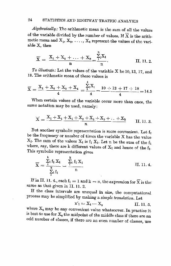
Algebraically: The arithmetic mean is the sum of all the values of the variable divided by the number of values. If 5 is the arithmetic mean and XV X2) X,, represent the values of the variable X, then
n
+xn EIXIX XI +X2 + I 11. 2. n n
To illustrate: Let the values of the variable X be 10, 13, 17, and 18. The arithmetic mean of these values is
4
- X1 + X2 + X3 + X4 EiXl 10 + 13 + 17 + 18X = 14.5 4 4 4
When certain values of the variable occur more than once, the same notation may be used, namely:
- - XI +X1 +X1 +X2 +X2 +X3 + +XkX II. 11. 3. n
But another symbolic representationis more convenient. Let ft be the frequency or number of times the variable X has the value XI. The sum of the values XI is ft XI. Let n be the sum of the ft where, say, there are k different values of XI and hence of the ft. This symbolic representation gives
k k
El ft XI El ft Xi II. 11. 4. X= I k - 1
El ft n
If in II. 11. 4., each ft = I and k = n, the expressionfor Y is the same as that given in II. 11. 2.
If the class intervals are unequal in size, the computational process may be simplified by making a simple translation. Let
x/I Xi - X0 II. where X0 may be any convenientvalue whatsoever. In practice it is best to use for X0 the midpoint of the middle class if there are an odd number of classes, if there are an even number of classes, use

25 SUMMARIZING OF DATA
the midpoint of a class as near the middle of the distribution as possible.
Substituting the value of Xi as given in IL I 1. 5. in equation IL 11. 4., we have
X
k
El f, Xi k
ff (X'i + XO)
k
El fj X'j
k
XOzi fl
n n n
k
Since Elf,nand k
Efj/n
k
X Xi fi X'l
XO +I -n
IL 11. 6.
In the special case when all class intervals are equal, we may use
the linear transformation (translation and change of unit)
Xi =Xi - X0 IL 11. 7. C
where c is the size of the class interval.
Using the value of Xi from IL 11. 7. in IL 11. 2.,
k
El ft (ex, + XO) X= 1
n
Y k k '0 El fjCXi fl Xi
n n
This when simplified becomes
k
X = XO + c 11.11. 8.
TO illustrate 11. 11. 8., we may use the frequency distribution
given in table IL 1.
26 STATISTICS AND HIGHWAY TRAFFIC ANALYSIS
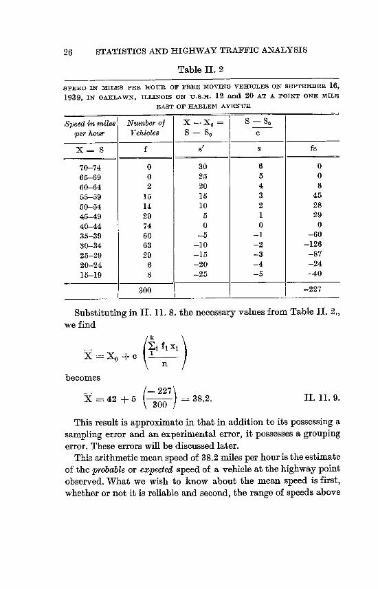
Table II. 2
SPEED IN MILES PER HOUR OF FREE MOVING VEHICLES ON SEPTEMBER 16,
1939, IN oAKLAwN, ILLINOIS ON U.S.H. 12 and 20 AT A POINT ONE MILE
EAST OF HARLEM AVENUE
Speed in miles Number of X -X, 8 - S,per hour Vehicles S S, C
X= S f S 8 fS
70-74 0 30 6 0 65-69 0 25 5 0 60-64 2 20 4 8 65-59 15 15 3 45 50-54 it 10 2 28 45-49 29 5 1 29 40-44 74 0 0 0 35-39 60 -5 -1 -60 30-34 63 -10 -2 -126 25-29 29 -15 -3 -87 20-24 6 -20 -4 -24 15-19 8 -25 -5 -40
300 -227
Substituting in IL 11. 8. the necessary values from Table IL 2.,
we find
k
X = X.0 + c
becomes
/- 227 X 42 + 5 30-0 ) 38.2. II. i I. 9.
This result is approximate in that in addition to its possessing a
sampling error and an experimental error, it possesses a grouping
error. These errors will be discussed later.
This arithmetic mean speed of 38.2 miles per hour is the estimate
of the probable or expected speed of a vehicle at the highway point
observed. What we wish to know about the mean speed is first,
whether or not it is reliable and second, the range of speeds above
27 SUMMARIZING OF DATA
or below it. Is 38.2 miles per hour characteristic for all vehicles and
if so, to what extent? We are able, with measures of dispersion, to find the answers to these questions. After doing this,'we must
look for a rational explanation of the agreement between the
statistically obtained values and the actual facts; we must also
determine what these facts mean. Were different types of vehicles
observed or was the variety of speeds due to drivers with different
desires or different abilities in driving, or to some other cause?
This will be discussed and illustrated in Chapter IV.
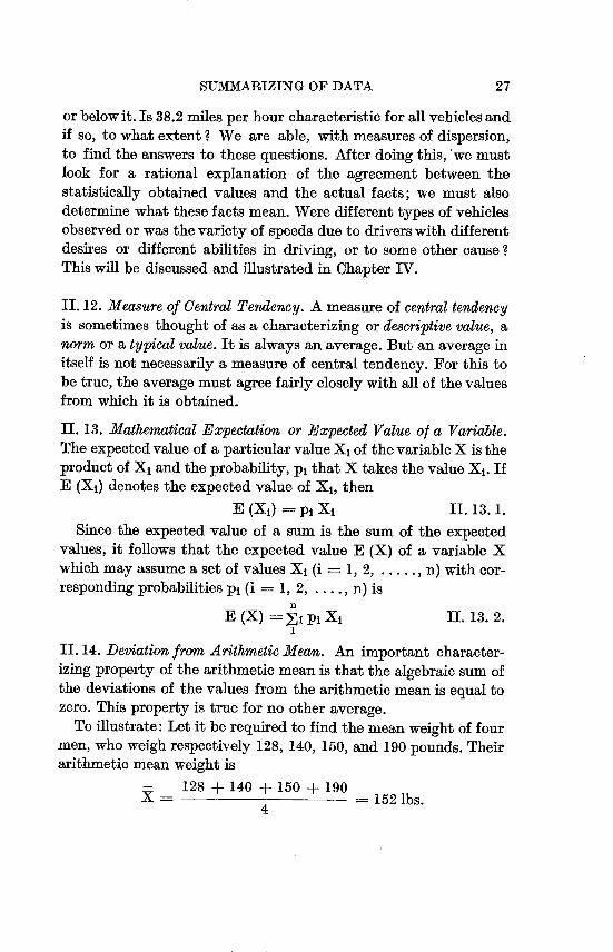
II. 12. Measure of Central Tendency. A measure of central tendency
is sometimes thought of as a characterizing or descriptive value, a
norm or a typical value. It is always an average. But an average in
itself is not necessarily a measure of central tendency. For this to be true, the average must agree fairly closely with all of the values
from which it is obtained.
II. 13. Mathematical Expectation or Expected Value of a Variable.
The expectedvalue of a particular valueXi of the variable X is the
product of Xi and the probability, pi that X takes the value Xi. If E (Xi) denotes the expected value of Xi, then
E (Xi) pi Xi 11.13.1.
Since the expected value of a sum is the sum of the expected
values, it follows that the expected value E (X) of a variable X
1
which may assume a set of values Xi (i = 1, 2 ....... n) with cor
responding probabilities pi (i 1, 2, n) is
E (X) El pi Xi 11. 13. 2.
H. 14. Deviation from Arithmetic Mean. An important character
izing property of the arithmeticmean is that the algebraic sum of
the deviations of the values from the arithmetic mean is equal to zero. This property is true for no other average.
To illustrate: Let it be required to find the mean weight of four
men, who weigh respectively 128, 140, 150, and 190 pounds. Their arithmetic mean weight is
- 128 + 140 + 150 + 190 X 4 152 lbs.

28 STATISTICS AND HIGHWAY TRAFFIC ANALYSIS
The differences between the individual weights of these four men and their arithmetic mean weight are:
Weights Algebraic Differences X XX 190 38 150 - 2 140 -12
128 - 24
Sum 0
The above demonstrationmay be stated in the form of a Theorem: The sum of the algebraic differences between the values of a variable X and their arithmetic mean X is equal to zero.
Let Xi (i 1, 2, . . ., k) be the values of the variable X, let f, (i = 1, 2, .. k) be the corresponding frequencies and let X be the arithmetic mean. Then
k - k kEl fi (XI - X) = El fl Xi _ X El fl. I 1 1
But k k
El f i n and 'Fl fi Xi = nX,1 1
Hence k
El fl (Xi - X) = nX - nX 0.I
This Theorem may be expressed in terms of mathematical expectation as follows: The expected value E I X - E (X) I of the, deviations of a variable from its expected value E (X) is zero, that is:
E f X - E (X)j 0 11.14.1.
Another characteristic of the arithmetic mean is its additive property. The meaning of this property may be made clear by finding the mean of two sets of given values. Let the first set be 115, 128, 140 and the second be 150, 190.
The arithmeticmean of thefirst set is 115 +128 +140 == 127 2/33

29 SUMMARIZING OF DATA
and of the second set is 150 + 190 170. The arithmetic mean of 2
115+128+140+150+190 the composite of thetwo sets i 144-1.
5
But the weighted arithmetic mean of the two arithmetic means
is
3 (1272) + 2 (170)3 144 3
3 + 2 5 '
This illustrates a theorem: The arithmetic mean of the sum of two
variables is the weighted arithmetic mean of their arithmetic means.
Symbolically: If XI is the arithmeticmean of the first set having nj
values and X2 is the arithmetic mean of the second set having n2
values and if Xi, + x, is the weighted arithmetic mean of the two
arithmetic means, then
n, XI + n2 X2 = -X, IL 14. 2. xi +,E. nj + n2
where X is the arithmeticmean of the n, + n2 values. This may be generalized to any number of variables.
In terms of expected values the theoremis stated as follows: The
expected value of the sum of two variables is the sum of their expected
values, that is:
E (XI + X2) = E (XI) + E (X2)' IL 14. 3.
To illustrate another theorem, reconsider the set of values 115,
128, 140. If we multiply each value by 2, we have the values 230,
256, 280. The arithmetic mean of 115, 128, 140 each multipliedby
2 is
230 + 256 + 280 = 2 1115 + 128 + 140 2 (1272)
3 3 1 = 3
The theorem is: The arithmetic mean of a constant times a variable
is equal to the constant times the arithmetic mean of the variable.
In terms of expected values the theoremis: The expected value of
a constant times a variable is equal to the product of the constant by the
expected value of the variable, that is:
E (ex) = CE (X) IL 14. 4.

30 STATISTICS AND HIGHWAY TRAFFIC ANALYSIS
Let us reconsider the arithmetic mean, namely: k
1i f, Xi f,
X _Xl + f2 X2 . ..... + fk Xk n n n n
k fj where 1i
1 n
It is important to note that the coefficients of the Xi, namely, the fi/n, are the relative frequencies of occurrence of these values.
But from the definitionof statisticalprobability(see ChapterIll), the limitingvalues of the fi/n, as n becomeslarge beyond all bounds, are the pi, where pi is the probabilityof occurrence of a value Xi of X among a set of mutually exclusive values Xi. Symbolically:
if, Xi E (X) lim X == lim 7,P1 Xi 11. 14.5.
ia . U- n where pi Xi is the expected value of a particularvalue Xi of X and El pi Xi is the sum of the expected values of the different particular values Xi of X. But the sum of expected values is the expectedvalue of the sum, and is calledthe mathematical expectation. It is also known as the probable or expected value of the variable.
It also follows from 11. 14. 5. that the arithmetic mean X of a sample is an approximation to the probable or expected value, namely, the true or universe value.
The arithmetic mean is most important in estimating and pre
dicting. The arithmetic mean X of a sample is the unbiased estimator (a value whose expected value is the true value) of the true mean of the population-thelatter being E (X).
To illustrate: Suppose we have a considerablenumber of observations of the speeds in milesper hour of vehiclespassinga givenpoint. These may vary, say, from 19 miles per hour up to 70 miles per hour. Suppose we wish to answer the question: At what speed in miles per hour wild - vehicle pass this point? The answer definitely is the expected value if we have the "universe", or the arithmetic mean if we have a random sample of the observed speeds. The arithmeticmean is the onlyone of the averages for a set of measure

31 SUMMARIZING OF DATA
ments that is an expected value. Furthermore, no quantity is of any real value for predicting purposes unless it is a probable or
expected value or unless as determined from a sample it is an
optimum or unbiased estimator. An optimum estimator is onethat
is consistent, efficient, and sufficient.
Another important theorem concerned with expected values is:
The expected value of the product of two mutually independent vari-
Wes is the product of their expected values. To illustrate:
Toss three pennies and throw three dice. The number of heads
occurring with the corresponding probabilities is shown in Table
H.3. Likewise, the number of one spots occurring with the corres
ponding probabilities is shown in Table H.3.
Table H.3
Pennies Dice
No. No. of of Heads Probability One spots Probability
X Pi Y P2
0 11/8 0 125/216
1 3/8 1 75 /216
2 3/8 2 "5/216
3 11/8 3 1/216
Table IIA
EXPECTED VAL-UES
Pennies Dice
X pi X Y P2 Y
0 0 0 0
1 3/8 1 75/216
2 6/8 2 30/216
3 3/8 3 3/216
E (X) 3/2 E (Y) 1/2
32 STATISTICS AND HIGHWAY TRAFFIC ANALYSIS
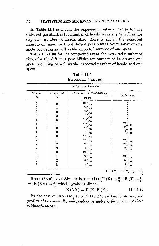
In Table IIA is shown the expected number of times for the
different possibilities for number of heads occurring as well as the
expected number of heads. Also, there is shown the expected
number of times for the different possibilities for number of one spots occurring as well as the expected number of one spots.
Table 11.5 lists for the compound event the expected number of
times for the different possibilities for number of heads and one
spots occurring as well as the expected number of heads and one
spots.
Table II. 5
EXPECTED VAL-UES
Dice and Pennies
Heads One Spot Compound Probability X Y A. P2 X Y PIP2
0 0 125/1728 0
0 1 76/1728 0
0 2 15/1728 0
0 3 "/1728 0
1 0 375/1728 0
1 1 225/1728 225/1728
1 2 4-5/1728 90/1728
1 3 3/1728 9/1728
2 0 37'/1728 0
2 1 225/1728 450/1711
2 2 45/1728 "'0/1728
2 3 3/1 728 11811728
3 0 125/1728 0
3 1 75/1728 225/1 728
3 2 15h728 90/1728
3 3 1/1728 9/1728
E (Xy) ..../1728 '/4
From the above tables, it is seen that [E (X) 3 [E (Y) I] [E (XY) fl which symbolically is,
4
E (XY) = E (X) E (Y). IL 14.6.
In the case of two samples of data: The arithmetic mean of the
product of two mutually independent variables is the product of their arithmetic means.

SUMMARIZING OF DATA 33
This theorem may be generalized to any -number of mutuallyin
dependent variables.
II. 15. The Deviations from Any Arbitrary Value. The arithmetic
mean of all the deviations from any arbitrary number, added to
that number is the arithmetic mean of the values. This theorem may be explained by considering the weights of five persons who
weigh respectively 135, 175, 180, 185, 190. Suppose we select
X0 = 180 as the arbitrary number, then
X f x X - X0 135 1 - 45
175 1 - 5
180 1 0
185 1 5
190 1 10
n 5 - 35
and K 180 - 355 173.
This is a much shorter method than adding all the items and
dividing by their number. Symbolicallythe theorem may be expressed as
X = X0 + Zx"/n
where
X0 = any arbitrary value but usually a guessed mean meaning
that it is as near the actual mean as can be estimated.
x" = deviation of each value from X0, the estimated mean.
n = number of cases (individual values).
11. 16. Mean Values in General. A Mean Value in general may be
thought of as the centroid of a frequency diagram. Let y = f (x)
be continuous in the x -interval (a, b).
Divide (a, b) into n equal parts, of length Ax and let yj (i = 1, 2,
.... I n) be the value taken by y in the ith part. The arithmetic
mean of the numbers yl, Y21 ., yn, that is
- Y1 + Y2 + + Y1 + + Yn y = II. 16. 1.
13

34 STATISTICS AND HIGHWAY TRAFFIC ANALYSIS
y
Xi
01 a ax b X
FIGURE II. 8
GRAPmcAL REPP.ESENTATION OF THE MEAN VALUE
will approach a definite limit as n tends to infinity. If the numerator and denominator of II. 16. 1. are multipliedby Ax, its forin is changed to
YJLAX + Y2A:K + + YIAX + + YnAX- IL 16. 2. nAx
But nAx = b - a and the area A under the curve between the limits a and b is
A Limit (y,_Ax + Y2AX + + YiAX + + YnAX) Ax-O n-w
=fb =fb
d A y d x.
Hence, the mean value - of y is n b
zi YjAx y d x y = Limit-! II. 16. 3.
n-. nAx b-a
Likewise, the mean value K of X is found by taking first moments about the y-axis, namely:
A X = fx d A., whence

35 SUMMARIZING OF DATA
b fxydx
b IL 16.4. f. Y d x
IL 16.2. may be interpreted as the average weight of nAx
objects having various weights where Ax objects have a weight of
yl, Ax have a weight of y2, .. ..
11. 16. 3. may also be obtained by the use of moments as illus
trated in Figure 11. 8. Here yiAx objects have, say, a distance xi.
The moment of yiAx about the y-axis is xiyiAx. The moment of n
the whole, if x- is its distance, is X_ (b - a) and also 1I Xi Yi Ax.
n b
Hence: X_ (b - a) liln xi yj Ax ydx,AX- 0
b xi yj Ax xydx
whence: X_ lim.,X-0 b-a b - a
The notion of mean is readily extended to functions of two or
more variables. To see this generalization, the reader is referred to
any book on Calculus or Mechanics.
IL 17. The Mode. The mode or modal value of a variable is that
value of a variable which occurs most frequently, if such a value
exists. It is the most probable value, or in other words, the value
for which the frequency is a maximum. The expressionmost prob
able value when it refers to the number of successes in n trials is
used in the general theory of probability to designate the number
to which there corresponds a larger probability of occurences than
to any other number. The point at which the frequency is most
dense is the abscissa of the maximum point of the frequency curve
and can be determined accurately only from the equation of the
curve.
For a given grouping the class mark of the maximal class frequency is called the empirical mode.
An approximation to the mode may be obtained by passing a
parabola through the midpoints of the upper bases of the modal
class and the two adjacent classes. Figure 11. 9. shows three such
points h, i, j.

36 STATISTICS AND HIGHWAY TRAFFIC ANALYSIS
The general equation of a parabola with its axis paxallel to the y-axis is
y OC + PX + yX2. H. 17. 1.
In Figure II. 9., take the origin at the point 0, namely, at the lower limit of the modal class. Let c equal the class interval and Aj. = OG and A2 = ED. When x = - c/2, y == 0; x = c/2, y = Al; x = 3 c/2, Y = Al. - A2- Substitute these values for x and y in II. 17. 1. and
0 a - P (c/2) + y 6")A 7)
.1 = a + P (c/2) + y (O' II. 17. 2.
Al - A2 = (X + P (3 c/2) + y (9
Solving these equations for oc, P, Y,
5 Al + A2. P ==Al A, +A2 II. 17. 3. 8 c y 2 C2
The maximum point on the curve y a + Px + yx2 is found by setting
dy/dx P + 2 yx = 0 IL 17. 4. d2y/dX2 2 y < 0
From II. 17. 4., x - P/2 y II. 17. 5.
y < 0
Substituting the values for P and y from II. 17. 3. in IL 17. 5.,
X Al c II. 17. 6. (Al +,A2)
The quantity found for x in II. 17. 6. when added to the lower limit of the modal class is the approximate value of the mode, namely
Mode + 0 II. 17. 7. (Al + A2)
where
13. lower limit of the class with maximum frequency.Al fo - fj (See Figure II. 9.)A2 Of - f, (See Figure II. 9.)

37 SUADLNRIZING OF DATA
In Table 11. I., fo = 74, f, = 60, f, 29. Substituting these values in II. 17. 7., we obtain
Mode == 39.5 + 14 \ 5 = 40.7. II. 17. 8. (14 + 451
The graphical counterpart of the solution just given for finding the modeis as follows. Considerthe distributiongiveninTableII. 1.
Y
T- D 7
60 h, 0C-\
50
4 0 CR
30 E J z +
20
10<
34.5 39.5 44.5 49.5
Speed in Miles Per Hour
FIGURE II. 9
GRAPHICAL SOLUTION
FOR FINDING THE MODAL VALUE OF A SET OF OBSERVATIONS
From this table select the modal class and the class adjacent to it on either side of it and for these three classes plot on graph paper these three frequency rectangles as illustratedin Figure II. 9.
38 STATISTICS AND HIGHWAY TRAFFIC ANALYSIS
Connect the points G and E with a straight line and the points 0 and D with a straightline. Then from the point of intersection of these two lines drop a perpendicular to the horizontal axis. The number read on the horizontal scale at the point where this perpendicular cuts the horizontal scale is the graphical solution of the mode. In this case it is 40. 8. Comparing the value of the mode found graphically with the value ofthe modejust found arithmetically, it is seen that the difference is 0.1, which is negligible.
It is not difficult to show, that the abscissa of the point of intersection of the lines joining OD and GE is
Al X = (A' + A) c
which proves that the graphical solution given is theoretically the same as the analytical.
It is obvious that for most practical purposes since graphically the value of the mode can be obtained with slight error the graphical solution of the mode will suffice. This result means that the most probable speed ofa vehicle at the pointobservedis 40.7 miles per hour. In other words, more vehicles pass this point at aspeed of 40.7 miles per hour than at any other speed.
II. 18. Median. The median of a variableis a numberwhichis such that half of the measurements have a value less than it and the otherhalf have a value greater than it. It is thus the abscissa of the point the vertical through which divides the total area under the frequency curve or frequency rectangles into two equal parts. To compute the median of a sample set of n values of the variable, computethe abscissa of a point, the vertical through which divides the total area of the frequency rectangles into two equal parts.
Illustration:
From columns (1) and (6) in Table II. I., and from Figure II. IO., it is seen that the sum of the frequencies (sum of the areas) of the classes up to X = 34.5 is 106 and the sum of the frequencies (sum of the areas) of the classes up to X = 39.5 is 166. But one-half the total frequency is 150 which is between 106 and 166. Hence the

39 SUMMARIZING OF DATA
fa
70
60 - -T
Z 50
40
E = 30 z
20
10
0i 10 aiCM CM M M .t 'n n
Speed in Miles Per Hour
FIGURE II. 10
MEDIAN VALUE OF OBSERVED VEMCLE SPEEDS
median value, by definition, lies between X = 34.5 and X 39.5
at a point which is the same proportion of the distance from
X 34.5 to X = 39.5 as 150 is from 106 to 166.
Symbolically it is seen that
Median + jn/2 - fel, c II. 18. 1. fm
where
11 lower bound of class in which median value falls.
n total frequency.
f,,, == cumulative frequency to lower limit of class in which median value lies.

40 STATISTICS AND HIGHWAY TRAFFIC ANALYSIS
f . = frequency of class in which median lies.c == length of class interval.Hence for the given distribution
Median = '34.5 + 150 - 106 5 38.2 II. 18. 2. 60
IL 19. Quantile8: Quantiles are location and division numbers. They, like the median, dividethe distributionintosections. There are many quantiles, but we shall mention and briefly discuss only those frequently used. There are the quartiles (quarters), quintile8 (fifths), decilm (tenths), and percentiles (hundredths). The method of finding them is similar to that of finding the median.
A quantile value (or percentile) is a number such that the specified quantile (percentage) proportion of cases have a measure less than it and the remainder have a measure greater than it. Symbolically,
1k n - f,Quantile = 11 + c II. I9. I.
where I lower bound of class in which quantile value falls. k proportion of cases below specified quantile value. n = total frequency. fp% cumulative frequency to lower limit of class in which
quantile value lies. fq == frequency of class in which the specified quantile value
lies. To illustrate: It is desired to find the lower quartile Q, or the
25th percentileand the upper quartile Q3 or the 75th percentile. In the former case, k ',4 and from columns (1) and (6) of Table
IL I., it is seen that f,1 = 43 and fq = 63 and 13L = 29.5. Hence II. 19. 1. becomes
Q1 = 29.5 + (1
4 (300)
63 - 43
5 ;:-- 32.0 11.19.2.
In the latter case, k == 43, it is seen that fj =. 166 and fq = 74
and 1, = 39.5. here II.19.1. becomes 43 (300) - 166
Q3 = 39.5 + . 5 43.5. II. 19.3. 74
SUMMARIZING OF DATA 41
These two values mean that 25 per cent of the vehiclesat the observed point had a speed less than 32.0 miles per hour and 25 per cent of the vehicles had a speed greater than 43.5 miles per hour.
If it is desired to know the 4th decile, then k 0.4 in IL 19. L and if it is desired to know the thirty-second percentile, then k 0.32. In other words the 4th decile means a speed such that 0.4 of the vehicles have a lower speed and 0.6 a higher speed and the thirty-second percentile means a speed such that 32 per cent have a lower speed and 68 per cent a greater speed.
Having found the values of the arithmetic mean, the median and the mode, what are the differences in their values and meanings ? It can be proved that the median value always lies between the arithmetic mean and the mode such that either
X : Median :9 Mode orMode ::: Median : Y IL 19.4.
For the distribution of Table IL L, it was found that 38.2., the Median 38.2., the Mode 40.7 miles per hour. The apparent equality of the median and arithmetic mean in this sample is due primarilyto grouping and sampling errors and to some extent due to experimental error. The modal value of 40.7 reveals that a greater proportion of the vehicles at the point observed travel at a speed greater than the probable or expected speed of 38.2 miles per hour. This observed tendency is important and can and must be explained from a subjective study. The other results show that 25 per cent of vehicles travelled with a speed less than 32.0 miles per hour and 25 per cent with a speed greater than 43.5 miles per hour and 50 per cent with a speed of from 32.0 to 43.5 miles per hour. The lower 25 per cent had a range in speed of 32.0 - 14.5 17.5 miles per hour, the middle 50 per cent had a range of 43.5 - 32.0 = 11.5 miles per hour, and the upper 25 per cent had a range in speed of 74.5 - 43.5 31.0 miles per hour. Similarly, the second 25 per cent had a range in speed of 38.2 - 32.0 = 6.2 miles per hour and the third 25 per cent a rangeof 43.5 - 38.2 = 5.3 miles per hour. These results indicaterather plainly a lack of stability and uniformity in speeds due to drivers, type of vehicles, and topography at point observed.

42 STATISTICS AND HIGHWAY TRAFFIC ANALYSIS
II. 20. Geometric Mean. The geometric mean of a set of n positive measurementsis the nth root of their product. If Xi (i = 1, 2, . . .. n) are the n values for a variable X, the geometric mean,
n I I
G.M. (rlxl)- II.20.1.I n = (XI-X2 X,)n-
where 11 is the symbol for the product. For a frequency distribution,
G.M. (Xfl- -Xf ..... Xfi ...... X kfk) U II. 20. 2.
where yif, = n. It is significant that the 1
log. G.M. fl 109X1 + f2 109X2 + + fk 'OgXk
n k It f, log Xi
11.20.3.
This means that the logarithm of the geometric mean is the arithmetic mean of the logarithms of the measurements. Recalling the relationship between relative frequency and probability, it is evident that as the number of measurements is indefinitely increased the logarithm of the geometric mean becomesthe probable or expected value of the logarithm of the variable X.
For analyzing a frequency distribution, the geometric mean has no immediate value. The geometric mean is the average of a set of rates and is the only average which is the average of a set of rates or the average of a set of things that behave like rates. Two examples will illustrate this property:
(1) A city had a population in 1900 of 100,000 and in 1910 of 120, 000. What is the average annualrate of increase in population? This problem is analogous to a problem in compound interest where the amount, principal, and time are known and the rate of interest is to be found. Hence
P. Po (I + r)n II.20.4. where
Pn the population at the end of n years.Po the population at the beginning of the period.n = number of time intervals.

43 SUMMARIZING OF DATA
Substitutethe above values in 11.20.4., then 120,000 100,000 (1 + r)10
Solving for r, it is found that
r .0184 = 1.84% change per annum.
(2) Given the information shown in tabular form:
Native Born Foreign Born Ratio of Ratio of Community Inhabitants Inhabitants Foreign Born Native Born to
to Native Born Foreign Born
A a = 9000 c = 4500 c/a = 50% a/c 200%
B b = 2000 d = 4000 d/b = 200% b/d 50%
It may be shown that the arithmetic mean is not the average
rate of increase.
The arithmetic mean of the ratios of Foreign Born to Native born is
50% + 200% c/a + d/b cb + ad = 125% = -
2 2 2 A
The arithmetic mean of the ratios of Native born to Foreign born is
200% + 50% a/c + b/d ad + bc = 125% = =-2 2 2 cd
Since the product of these two results is not unity or I 00 %, they
axe illogical and the arithmetic mean is not the proper average to use.
The geometric mean of the ratios of Foreign born to Native born is
G.M. = V.50 -2.00 = 1.00 == 100 % = Y/a-- d/b = Ycd/ab.
The geometric mean of the ratios of Native born to Foreign born is
G.M. F2.00 -.50 1.00 I00 % Va/c -b/d = Yab/cd

44 STATISTICS AND HIGHWAY TRAFFIC ANALYSIS
The product of these two results is unity or 100%. c + d 4500 + 4000 8500
Now --+ b 9000 + 2000 11000 = .7727 = 77.27% and
a + b 9000 + 2000 11000 1.2941 129.41 %.
-+-d 4500 + 4000 8500
But c + d.a + b I and .7727 times 1.2941 1. a + b - -+d
Since the product of the ratios mustbe unity, it is seen that the geometric mean is ae average rate.
II. 21. Harmonic Mean. The harmonic mean of a set of measures is the reciprocal of the arithmetic mean of the reciprocals of the measures.
Symbolically, if H M. is the harmonic mean,
H.M.' II. 21. 1. f1/X1 + f2/X2 + + fk/Xk
To illustrate: Suppose we have a vehicle that travels 25 miles per hour for 20 miles, then 30 miles per hour for 10 miles, then 50 miles per hour for 50 miles, then 40 miles per hour for 10 miles and finally, 12 miles per hour for 10 miles. What is the average speed of this vehicle for the I 00 miles travelled? It is the harmonic mean, namely,
H.M. = 100 20 (1/25) + 10 (1/30) + 50 (1/50) + 10 (1/40) + 10 (1/12)
31.1 miles per hour. This average speedmay be found by an arithmeticmean method
if weights are properly chosen. If X' is the symbol for the average speed for an arithmetic mean method,
251(.04) (20))+301(.033) (10))+501(.02)(50)1+401(.025)(10))+121(.083)(10))
3.2125 (.8) + 30 (.333) + 50 (1) + 40 (.25) + 12 (.833)
3.21 20.000 + 9.999 + 50.000 + 10.000 + 9.996
= 31.1milesperhour3.21
where 0.8, 0.333, 1, 0.25, and 0.833 axe the weights.

45 SUMMARIZING OF DATA
The latter method, while it solves the problem, is not as direct and
simple as the harmonic mean. Of all the averages, the harmonic
mean is the only one that is the average time rate orae average
of things that behave like time rates.
II.22. RootMeanSquare.TherootmeansquareR.M.S.,aoftencalled
thestandarddeviationin statisticsis similarto theradius ofgyration k
in mechanics.The radius of gyrationof the area under a frequency
curve about the ordinate through the center of gravity of that
area is, in fact, equal to a. The physical meaning of radius of gyrationis that it is a distance
such that if all the mass of a body (or area) were concentrated at a
point that distance from an axis of rotation it would have the
-same rotational effect as the actual distributed mass (area). It is
also the root meansquare of the radial distances of a set of n equal
particles from an axis. In the same way, a, the standard deviation
,of a frequency distribution (area) thought of as a set of n equal
particles of area is the square root of the arithmetic mean of the
squares of the radial distances of the several particles from the centroidal axis, that is, it is the R.M. S. as well as k with respect
to the centroidal axis.
It is believedthat a review of the significanceof second moments
and the radius of gyration k in mechanicswill help to understand
the correspondingterms in statistics.
Let A be any area and YY an axis through the centroid 0 as
shown in Figure II. 1 1.
Let dA represent an element of area and let x be its distance
from the centroidal axis YY. The moment of inertia Iy is by definition the sum of all the
x2 dA, that is,
IY = f6.x 2 CIA II. 22. 1.
and the radius of gyration,
k 2 = IY 11. 22. 2. A
If the moment of inertia of an area with respect to a centroidal
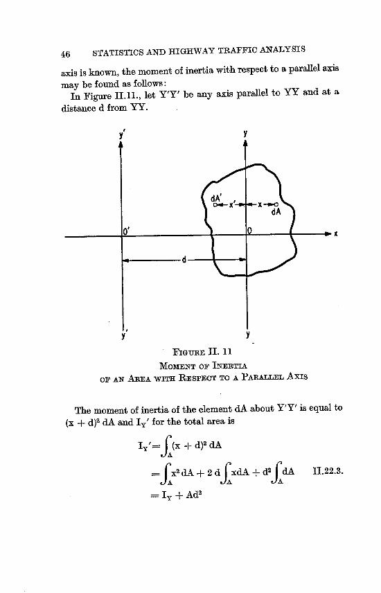
46 STATISTICS AND HIGHWAY TRAFFIC ANALYSIS
axis is known, the moment of inertia with respect to a parallelaxis
may be found as follows: In Figure 11. II., let Y'Y' be any axis parallel to YY and at a
distance d from YY.
y y
d X
dA
of 0
d
y y
FIGURE II. 11
MOMENT OF INERTIAOF Ax AREA W RESPECT TO A PARALLEL Axis
The moment of inertiaof the element dA about Y'Y' is equal to (x + d)2 dA and lyI for the total area is
ly'=fA(x + d)2 dA
)0 dA + 2 d dA + d2 dA 11.22.3. =1 fAX fA
= ly + Ad2

SUMMARIZING OF DATA 47
since dA = Ai = 0. JAX
The fact that fAxdA 0 may be comprehended if it is re
membered that for every element dA on the right, there is an
element (d.A)' at a distance x' to the left, such that x' (dA)' = xdA.
In other words, we may think of the area as being balanced about
the centroidal axis.
The frequency diagram in statistics may be treated in the
same manner as an area is treated in mechanics. The notation is
slightly different and so is the point of view and interpretation as
is shown in Figure II. 12. Oth6rwise, the procedure is the same.
V
unit
xi-X X
FIGuRF, IL 12
Fp.iQuENcy DIAGRAM
Using the notation shown in Figure II.12. a2=k2= 12 II.22.4.
I/n) (xi - X-/
This may be written in the form
n 2 a2 = 2 k2 (1/n2) Zj (Xi - Xj)2 II.22.5.
1
We thus see that the standard deviation is (1) the square root
of the arithmetic mean of the squares of the differences between
the measurements and their arithmetic mean and (2) proportional
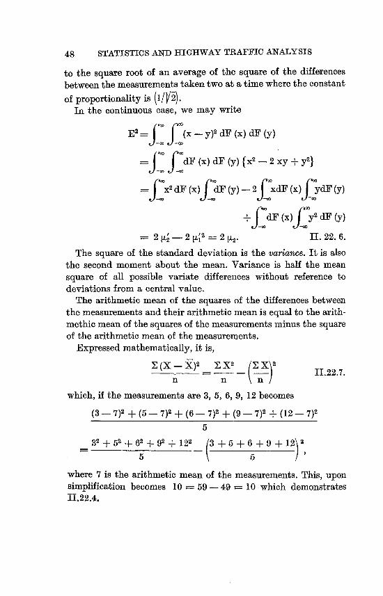
48 STATISTICS AND HIGHWAY TRAFFIC ANALYSIS
to the square root of an average of the square of the differences betweenthe measurementstakentwo at a time where the constant
of proportionality is (I/Y2. In the continuous case, we may write
E 2 E (x - y)l dF (x) dF (y)00
f dF (x) dF (y) fX2 - 2 xy + y2l=f
=fX2 dF (x)f - 2 dF (x) 'O dF (y)X y
+fdF (x) y2 dF (y)f
2[t'- 2 2 II. 22. 6.
The square of the standard deviation is the variance. It is also the second moment about the mean. Variance is half the mean square of all possible variate differences without reference to deviations from a central value.
The arithmetic mean of the squares of the differences between the measurements and their arithmetic mean is equal to the arithmethic mean of the squares of the measurements minus the square of the arithmetic mean of the measurements.
Expressed mathematically, it is,
E (X 5)2 EX2_ EX2 JI.22.7.
n n n I
which, if the measurements are 3, 5, 6, 9, 12 becomes
(3 - 7)2 + (5 - 7)2 + (6 - 7)2 + (9 - 7)2 + (12 - 7)2
5
32 + 52 + 62 + 92+122_(3+5+6+9+12 2
5 5 ) ,
where 7 is the arithmetic mean of the measurements. This, upon simplification becomes 10 = 59 - 49 == 10 which demonstrates 11.22.4.

49 SUMMARIZING OF DATA
Also
1(3-3)2 + (3-5)2 + (3-6)2 + (3 - 9)2 + (3-12)2 + (,5-3)2
* (5 - 5)2 + (15 - 6)2 + (5 - 9)2 + (5 - 12)2 + (6- 3)2 + (6-5)2
* (6- 6)2 + (6- 9)2 + (6 - 12)2 + (9 - 3)2 + (9-5)2 +(9-6)2 * (9 - 9)2 + (9 - 12)2 + (12 - 3)2 + (12 - 5)2 + (12 - 6)2
* (12 - 9)2 + (12 - 12)21 '. (5) (5) 52050 = 20 -- 2 (10).
Hence 2 a2 = j:jj (Xi - Xj)2 becomes 2 (10) = 20
which demonstrates II.22.5.
In case we have k values of Xi and each value occurs several
times, or in case we have a frequency distributionwhere Xi is the
class mark of the ith class and f, is the frequency of the ith class, it is convenient to write
i fi (Xi X)
2 I fj Xi
2 I ft Xi
2
II.22.8 n n n
Considering the limit definition of probability, namely,
Limit fl/n pi, we have
n- 00 E [(X - E (X)2 E (X2 [E (X)] 2 11.22.9.
which in words is the theorem: The expected value of the square of
the deviation of the variablefrom the expected value is equal to the ex
pected value of the, square of the variable minus the square of the ex
pected value of the variable.
In the special case when the class intervals are all equal, we may use the value of Xi from II. II. 7. in 11. 22.8 and then
k - 2 2y1fi (Xi_ X n 2 I f, X12
a C, ff Xi
n II.22.10. n n
To illustrate, consider the distributiongiven in columns (1) and (2)
of Table II. 1. and the tabulation as shown in Table II.6.
Making use of formula II.22.10., namely,
a = CVEfS2 _ Zfs)2
_n _n
where now X S and x = s
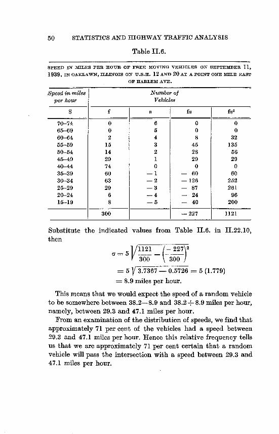
50 STATISTICS AND HIGHWAY TRAFFIC ANALYSIS
Table 11.6.
SPEED IN MILES PER HOUR OF FREE MOVING VEHICLES ON SEPTEMBER
1939, IN OAXLAWN, ILLINOIS ON U.S.H. 12 AND 20 AT APOINT ONE Mrr EAST
OF HARLEM AVE.
Speed in mile8 Number of per hour Vehicles
S f 8 fS f§2
70-74 0 6 0 0 65--69 0 5 0 0 60-64 2 4 8 32 55-59 15 3 45 135 50-54 14 2 28 56 45-49 29 1 29 29 40-44 74 0 0 0 35-39 60 - 1 - 60 60 30-34 63 - 2 - 126 252 2&-29 29 - 3 - 87 261 20-24 6 - 4 - 24 96 15-19 8 - 5 - 40 200
300 - 227 1121
Substitute the indicated values from Table IIA in II.22.10,
then
.5 VI 121 2272
30-0 300
5 V 3.7367 - 0.15726 = 5 (1.779)
8.9 miles per hour.
This means that we would expect the speed of a random vehicle
to be somewhere between 38.2 - 8.9 and 38.2 + 8.9 miles per hour,
namely, between 29.3 and 47.1 miles per hour.
From an examinationof the distribution of speeds, we find that
approximately 71 per cent of the vehicles had a speed between 29.3 and 47.1 miles per hour. Hence this relative frequency tells
us that we axe approximately 71 per cent certain that a random
vehicle will pass the intersection with a speed between 29.3 and 47.1 miles per hour.
51 SUMMARIZING OF DATA
If on the other hand, we use the expected speed of 38.2 miles
per hour as our estimate, it is 71 per cent certain that we will be
in error by at most afX_ == 8.9/38.2 = 23.3 per cent. On the other
hand, it is 29 per cent certain that the error is at least 23.3 per cent.
This indicates that there is marked variability in speeds and
there does not appear to be a typical speed at all for this point on the highway.
IL 23. Centra HarmonicMean. The centra harmonic mean is a meas
ure of relative dispersion. It is the arithmetic mean of the squares
of the measures from an arbitraryorigin dividedby the arithmetic
mean of the measures. Symbolically if C.H.M. is the centra harmonic mean, then
n n C.H.M. X?/ xi. 11.23.1.
The centra harmonic mean per se is of very little use today.
However, a quantity similar to it, namely the coefficient of vari
ability is useful as a measure of relativedispersion or a measure of
per cent of error. If C.V. is the symbol for coefficient of variability, then, by definition
n n
i (Xi - X), El xi a C.17. I1.23.2.
n n X
In II.22. the CY. was interpreted for the distribution given in Table IL L
IL 24. Mean or Average Deviation. The mean or average deviation
from an average is the A.M. of the deviations treating them all as
positive. The deviations may be taken from any average, but the
mean deviation is least whenthe median is the origin.
In case of a normal distribution with origin at the arithmetic
mean or median, the mean deviationis the abscissa of the centroid
of area under the right hand half of the frequency curve and its
value is 0.7978 a = 0.8 a approximately. Assume the frequency
for each class concentrated at the center of class as shown in
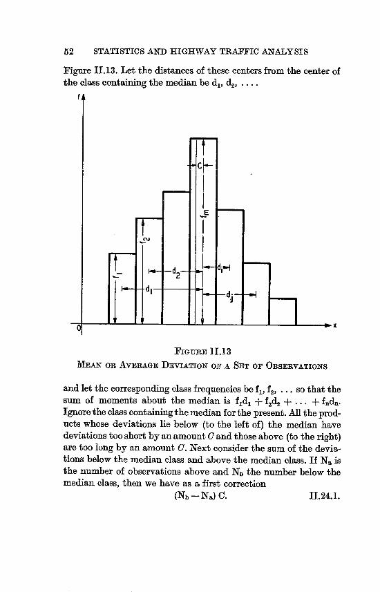
52 STATISTICS AND HIGHWAY TRAFFIC ANALYSIS
Figure II. 13. Let the distances of these centers from the center of the class containing the median be dj, d, .....
f
cm
-d2
dj
0i XFiGURE II. 13
AIEAN OR AVERAGE DEviATioN OF A SET OF OBSERVATIONS
and let the correspondingclass frequencies be f,, f2l ... so that the sum of moments about the median is f1d, + f2d2 + - - - + fndn-
Ignore the class containingthe medianfor the present. All theproducts whose deviations lie below (to the left of) the median have deviations tooshort by anamount C andthose above (to the right) are too long by an amount C. Next consider the sum of the deviations bestow the median class and above the median class. If N" is the number of observations above and Nb the number below the median class, then we have as a first correction
(Nb - NO C. II. 24.1.

53 SUMMARIZING OF DATA
If Nrn is number of observations in the median class and if we
assume these Nm observations uniformly distributed over the
interval, then (.5 + Q N. cases are below and (.5 - Q Nm are
above the median. With a uniform distribution, the sum of these
deviations below the median is
(.5 + C)2 Nm and above the median (.5 - Q2 Nru 2 2
Hence the sum of all the deviations of the Nm values is
(.5 + C)2 N., + (.5 - C)2 N., = (.25 + C2) Nm. II.24.2. 2 2
which is the second correction.
Let us now find the mean deviation from the median for the
distributiongiven in Table II.I.
Table II. 7.
SPEED IN MILES PER HOUR OF FREE MOVING VEHICLES ON SEPTEMBER 16, 1939, IN OA KI AWN, ILLINOIS, ON U.S.H. 12 AND 20 AT A POINT ONE MILE EAST
OF HARLEM AVE.
X = S f X = 8 fjSj*
70-74 0 7 0 65--69 0 6 0 60-64 2 5 10 55-59 15 4 60 50-54 14 3 42 45-49 29 2 58 40-44 74 1 74 35-39 60 0 0 30-34 63 - 1 63 25-29 29 - 2 58 20-24 6 - 3 18 15-19 8 - 4 32
300 n 415
The symbol Isl means the numerical value of s which is always positive or zero.

64 STATISTICS AND HIGHWAY TRAFFIC ANALYSIS
Correction (1): (Nb -N,) C= (106 - 134) (1.2) - 33.6 Correction(2): (.25+C2)Nm=(.25+1.44)(60)= 101.4 Sum of deviations for classes other than median class 415.0
Sum of all deviations 482.8 482.8
Mean Deviation - = 1.609 class intervals 300
8.05 8.1 miles per hour. This means that the expected value of the difference between
the speed of a vehicle and the median value of speeds is 8.1 miles per hour.
Given N values. Choose a certain number as origin such that x of the values will be greater than this number. Then N - x will be less than the selected number. Let the deviations from the selected number (average) as origin be A. Displace the original origin by K units so that it is exceeded by only x - 1 values. Then N - (x - 1) of the values will be less than the new number. By this change, the sum of the deviations in excess of the selected number is decreased by Kx, while the sum of the deviations less than the selected number is increased by (N - x) K. If A' is the new sum of deviations, then
A' A + (N - x) K - I%'-x and A' A + (N - 2 x) K. If x = N/2; 4' = A. lf x > N/2; A' < A.
This proves that the sum of the numerical values of the deviations from the median is a minimum.
II. 25. Moments and Mathematical Expectation of Powers of a Variable.
The moments of a distribution are the expected values of the powers of the stochastic variable which has the givendistribution. The term "moment" has been taken over by the statistician from mechanics. In mechanics, moment is a measure of a force with respect to its tendencyto produce rotation. In statistics moments characterize the parameters of the distributionlaw which are the properties that describe for interpretation and meaning the law of behavior of the attribute that is being measured and studied.

55 SUMMARIZING OF DATA
The late Karl Pearson (Biometrika, Vol. 9, pp. 1-10) has shown
that all the constants of a frequency distributionare expressible in
terms of higher productmoments. In the case of two variates, they
are defined by n
Vq, q' -- yij fplj X1q Yjq') II.25.1. 1
for an arbitrary origin. If the origin is at the mean, namely, at
P (-x, -y), then
yij ( Pij (Xi _ -)q (yj )ql11% q, I x y II.25.2.
In case of a single variable, the k th moment of a continuous
variable x about an arbitrary origin denoted by vk is
b
,vk = E (Xk) =- Xk f (x) dx II.25.3.
and in the case of a discontinous variable x
n 'Vk = E (Xk) Epi Xjk. II.25.4.
As has been seen, the first moment about an arbitrary originis
the probable or expected value and in case of a sample it is the
arithmetic mean of the x values.
The k th moment of the variable x about an arbitrary point a is
defined as b
E [(X - a)k] f- (x - a)k f (x) dx II.25.5.
or
E [(x - a)k] (xi - a)k pi. II.25.6.
If a is the arithmetic mean -X of x and if Lk is the symbol for the
k th moment about the mean, then
b
ilk= E [(x - 3E)k] = E [(x - vj)k] =f (X - V1)k f(x) dx II.25.7.
or
Ilk = E [(x - Vl)k] Y_,pi (Xi - VI)k. II.25.8. 1
It is not hard to see that CF2

56 STATISTICS AND HIGHWAY TRAFFIC ANALYSIS
It is easy to show that the moments about the mean can be ex
pressed in terms of the moments about an arbitrary origin. These
relations are: k b
[tr z! pi (xi - VIY =f. (x _ Vj)r f(x) dx II.25.9.
Specifically: PO
Ili 0
f12 V2 - "I2
'3 V3 - 3 VI V2 + 2 v,3
P-4 = v4 - 4 v3 v3 + 6 v.2V2 - 3 VI4 II.25.10.
............................
r r! tLr= VI)l vr-, , where . . namely the,
i! (r - i)!0 i)
number of combinations of r things taken i at a time.
For a sample
k
Vr Zi ft XiUn1.
k
and [L, 1i fi (Xi - X)r/n. II.25.12. I
Now consider the translation x'- X - X0, and if vr the
rth moment of x', then
k
k Zi f, (xi)t V, 1,i f, (Xi - X,)'/n = 1 - , Vr II.25.13.
I n
and similarly if x X-XO and v" is the rth moment of x r c
k ky,,f, (cx)r er Z if, Xr
Vr= II.25.14. n n
Hence:
[Ir (- Vi) Vr_1 II.25.15. 0 1

SUMMARIZING OF DATA 57
and
cr JJ.25.16.
To illustrate: Consider the distribution of Table II.I. and find thefirst four moments about the mean using 11.25.10 and II.25.16.
Table II.S.
SPEED IN MILES PER HOUR OF FREE MOVING VEHICLES ON SEPTEMBER 16,
1939 IN oAxLA-,vw, ILLINOIS, ox U.S.H. 12 AND 20 AT A POINT ONE MILE EAST
OF HARLEM AVENUE
S f 8 fS fS2 fS3 f,4
70-74 0 6 0 0 0 0 65-69 0 5 0 0 0 0 60-64 2 4 8 32 128 512 55-59 15 3 45 135 405 1215 50-54 14 2 28 56 112 224 45--49 29 1 29 29 29 29 40-44 74 0 0 0 0 0 35-39 60 -1 -60 60 -60 60 30-34 63 -2 -126 252 -504 1008 25-29 29 -3 -87 261 -783 2349 20-24 6 -4 -24 96 -384 1536 15-19 8 -5 -40 200 -1000 5000
300=n -227 1121 -2057 11933
From Table II.S.
VO
VJLI/ - 227 = - 0.75667 300
1121 V211 - 3.73667300
- 2057 V311 = 6.85667300
11933 V4/1 = 39.77667300
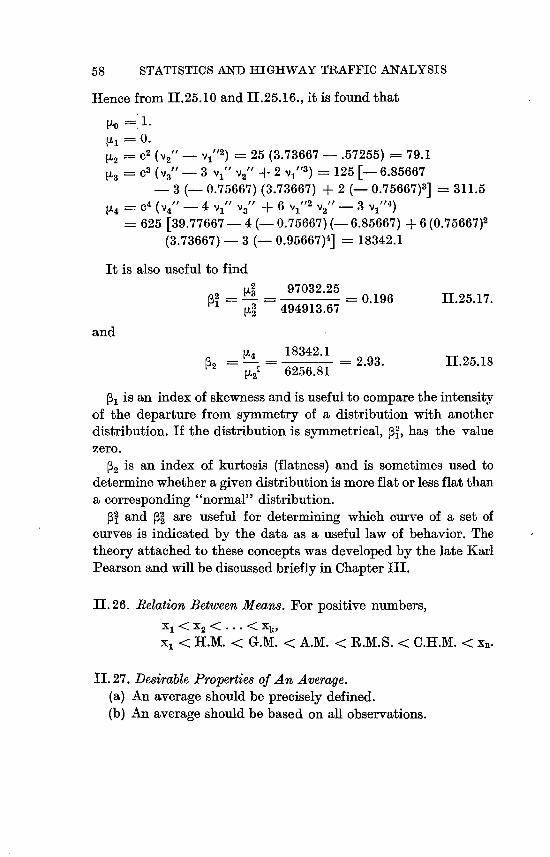
58 STATISTICS AND HIGHWAY TRAFFIC ANALYSIS
Hence from II.25.10 and II.25.16., it is found that
[Lo
[I, = 0
tL2 c20211 - V1112) = 25 (3.73667 -. 57255) = 79.1
tL3 = C3 03" - 3 VI" V2" + 2 vj'13) 125 [- 6.85667 - 3 (- 0.75667) (3.73667) + 2 (- 0.75667)q 311.5
114 = O 041' - 4 vlf 1 'V3" + 6 ,,"2 V21' - 3 VI/14)
625 [39.77667 - 4 0.75667) (- 6.85667) + 6 (0.75667 )2
(3.73667) - 3 0.95667)4] 18342.1
It is also useful to find 2
p2 M 97032.25 1 3 494913.67 0.196 II.25.17.
112
and
114 18342.1 P2 = 2.93. II.25.18
IZ2 6256.81
p, is an index of skewness and is useful to compare the intensity
of the departure from symmetry of a distribution with another
distribution. If the distributionis symmetrical, p2 has the value
zero.
P2 is an index of kurtosis (flatness) and is sometimes used to
determine whether a given distributionis more flat or less flat than
a corresponding "normal" distribution. P21 and P22 are useful for determining which curve of a set of
curves is indicated by the data as a useful law of behavior. The
theory attached to these concepts was developed by the late Karl
Pearson and will be discussed brieflyin Chapter III.
II. 26. Relation Between Means. For positive numbers,
XI < X2 < . . . < Xk,
xi < H.M. < G.M. < A.M. < R.M.S. < C.H.M. < Xn-
II. 27. Desirable Properties of An Average.
(a) An average should be precisely defined.
(b) An average should be based on all observations.

59 SUMMARIZING OF DATA
(c) An average should possess some simple and obvious properties to render its general nature comprehensible: it should not be too abstract in mathematical characterization.
(d) An average should be possibleof easy and rapidcalculation. (e) It should be as little affected as maybe possible by fluctua
tion8 of sampling or by sampling errors. (f) The measure chosen shouldlend itself to algebraic treatment
and its basis should be concordant with the basis of the problems to be analyzed.
These properties applied to the mean, median, and mode, geometric mean, and harmonic mean are:
I. ArithmeticMean. The A.M. satisfies a, b, c, d, e, f. The arithmetic mean has the following properties.
(a) The sum of the deviations from the mean, taken with their proper signs is zero.
(b) The mean of a whole series can be readily expressedin terms of the means of its components.
(c) The mean of all the sums or differences of corresponding observations in two series (of equalnumbers of observations) is equal to the sum or difference of the means of the two series.
(d) The sum of squares of the deviations from the arithmetic mean is a minimum.
IL Median. The median satisfies (b) and (c) but the definition does not necessarily lead in all cases to a determinate result. The median is easier to compute than the arithmetic mean. The arithmetic mean is superior to median in lending itself to algebraic treatment. No theorem for median exists similar to (b) for mean and likewise to (c). The medianhas the, following advantages over the mean:
(a) It is very readily calculated: a factor to which, however, as already stated, too much weight ought not to be attached.
(b) It is readily obtained without necessity of measuring all objects to be observed.
(c) Sum of the deviations from Median, all > 0, is a minimum. III. Mode. What wewant to arrive atis the mid-value of the inter
val for which the frequency would be a maximum, if the intervals

60 STATISTICS AND HIGHWAY TRAFFIC ANALYSIS
could be made indefinitely small and at the same time their number be so increased that the class frequency would run smoothly. A smoothing process is necessary; viz. that of fitting an ideal frequency curve of given equation to actual figures.
IV. Geometric Mean. The geometric mean is used in averaging rates or ratios rather than quantities.
(a) If the ratios of the geometric average to the measures it exceeds or equals be multiplied together, the product will be equal to the product of the ratios of the geometric average to those measures which exceed it in value.
If XI < X2 < X3 < ... < Xk < G.M. < Xk+1 < X11+2 < ... < Xnl
G G G Xk+I Xk+2 Xnthen, - - - . . . . . - = - -- 11.27.1. XI X2 Xk G G -6
(b) The geometric average of the ratios of corresponding observations in two series is equal to the ratio of their geometric averages.
(C) The geometric average of the series formed by combining n different series each with the same frequency is the geometric average of the geometric averages of the separate series.
V. Harmonic Mean. The harmonic average of a set of measurements must be used in the averaging of time rates.
Having shownthe initialprocedurenecessaryfor a statisticalanalysis, namely, how to summarize data and how to obtain summary numbers for the purpose of characterizing the law of behavior of the observedfacts, we shall now develop the necessary theory that is basic for the analysis and solution of traffic problems.
REFERENCES, CHAPTER II
Yule, G. Udney, and Kendall, M. C., "An Introduction to the Theory
of Statistics," C. Griffin &.Co., London, 1937.
2 Croxton, F. E., and Cowden, D. J., "Applied General Statistics," Pren
tiss-Hall Inc., New York, 1946.
3 Rider, Paul, "Statistical Methods," John Wiley & Sons Inc., New York,
1939.
4 Kendall, M. C., "The, Advanced Theory of Statistics," Charles Griffin
& Co., London, 1946, Vol. 1.

CHAPTER III
STANDARD DISTRIBUTIONSAND THEIR MATHEMATICAL PATTERNS
III. I-Objective. The purpose of this chapteris to explaintherelated
problems of first ascertainingthe nature of a universeof events and
second finding a mathematical model or pattern that fits the
universe. From experience and intuition, we know that a sample will tell us something about the entire series of events, and that
the larger the sample the more accurately it reflects the character
istics of the parent universe. We reasonthat a mathematicalmodel of the sample, if the sample is large, will also be a model of the
universe. Obviously, this fitting of mathematical patterns will be
much easier if we know something about the types of universes or
distributions of events we may expect to find.
There are three of these theoretical distributionsthat constitute
the basic patterns. They are, in the order of their discovery, the
Binomial (James Bernoulli about 1700), the Normal (Demoivre
about 1700, Laplace and Gauss about 1800), and the Poisson (B.D.
Poisson about 1837). Other distribution patterns have been dis
cussed by Gram (1879), Fechner (1897), Thiele (1900), Edgeworth
(1904), Charlier (1905), Brun (1906), Romanowsky (1924), and
others. These are in general either other approaches to, modifica
tions, or generalizations of the three basic distributions. The most
logical order to present these from the standpoint of clearnessis
also the historicalorder of appearance. But before consideringthe
first of these, the Binomial distribution, we shall discuss the ele
ments that make up a distribution.
111.2. The Elements of a Distribution. In order to'/.define and to point
out the interrelationshipsof the elements that make up a distri
bution, let us consider a trial like the throwing of a die. The result will be the happening or non-happening of a specific event such as
the falling of the die with one spot on the top face.
An event, of course, can be the occurrence of any attribute or
61

62 STATISTICS AND HIGHWAY TRAFFIC ANALYSIS
characteristic as well as a happening. In traffic, for example, it
could be the age of a driver, his seeing ability, the life of an auto
mobile tire, the weight class of a truck, the volume of traffic, the
speed of a vehicle, or any one of many other things. The happeningof a specific thing is called the Event E, and the
non-happening is called the complementary event B. If the die is
thrown a limited number of times (number of trials), we get a
sample distribution of B's and B's. If the number of trials is increased withoutlimit, the observed sample distributionapproaches
the true or theoretical distribution of the univer8e or total popula
tion of the events.
There are thus two kinds of distributions: (a) the theoretical
and (b) the experimentalor sample distribution.
The Theoretical Di8tribution: In order to explain the theoretical
distribution, let f t be the number of ways in which the event E can
take place, f, the number of ways for the complementary event E,
and n the total number of trials or happenings and non-happen
ings.
The probability that the event.E will occur is the ratio of the
number of ways ft in which E can happen to the total number of
possible and equally likely happenings and non-happenings. Let
p or P (E) be this probability, then symbolically
p = P (E) = ft/n
Similarly, the total number of ways f, in which the event E can
happen divided by n is defined as the probability (a-priori, true, or
theoretical) that the event E will occur. Let q or P (E) be this
probability, then symbolically
n-ft ft q = P (E) = f,/n = = I __. III.2.2.
n n
In the case of a die, if E is the event of the die's falling with one-
spot on the top face and E is the event of the die's falling some
other way, then ftl, fc=5, n6
and
p=P(E)=';q=.P(E)=1; and p+q=' +5 1.6 6 6 6

63 STANDARD DISTRIBUTIONS
Again if n is the total number of registered vehicles and ft is the
number of light trucks, then
p = P (E) n
is the true probability that a vehicle is a truck.
In general, let a be the number of times the eventE occurs, and
let b be the number of times the event R occurs, these being the
only possibilities. Then p = a/(a + b) is the probability that the event happens as specified - event E, and q b/(a + b) is the
probability that the event does not occur - event E. It follows that
p + q 1, which simply demonstrates what we know intuitively
that an event is certain to happen or not to happen. This also
shows that both p and q are positive numbers. This is the Funda
mental additive property in probability. This property is also re
ferred to in the literature as the Rule of Complementation.
Let us Dow suppose that one tosses a penny twice and wishes to
find the probabilityof getting two heads. One might reason falsely that there are three possibilities: two heads, two tails, or one head
and one tail. One of these outcomes is two heads, therefore, one
might reason that the probability is "T, but this reasoning is false,
for the events are not equally likely. The third event may occur in
two ways for a head could appear on the first trial and the tail on
the second, or the head could appear on the second and the tail on the first. There are really four equally likely outcomes or phases:
HH, HT, TH, TT; and the correct probabilityis therefore f. The
four events are independent and mutually exclusive. If two heads
axe up, that is the only possible combination, for if a penny is
heads up, it obviously cannot at the same time be tails up. This
mutual exclusiveness does not always exist. Suppose that one
wishes to compute the probability of drawing a king or a heart
from a deck of cards. The chances might be Assumed to be 1I7
since there are 4 kings and 13 hearts. But this is incorrect, for the
drawing of a king does not exclude drawing of a heart. The king
may also be a heart.
The Experimental Di8tribution: The experimental or sample
distribution is obtained from a number of observations of events.
64 STATISTICS AND HIGHWAY TRAFFIC ANALYSIS
Let fo be the number of times the event E is observed to happen and n the total number of trials or observations. The ratio fo/n is
called the relative frequency of the event E and 1 - f0 is the relanL)
tive frequency of the event E. The obtaining of the numerical values of the relative frequencies
fo/n is actually a very simple problem since it is essentially a problem of counting. The value of fo/n in contrast to the true probability varies with the number of observations or trials n. One might count all the traffic violations that occurred at an intersection during the passing of 5000 vehicles and find that there were no violations. In this situation, the observed fo = 0, n 5000 and fo/n = 0/5000 equals zero. But if the violations occurring during the passing of 25000 vehicles were counted, it might be found that there were 4 violations, and now the observed fo = 4, n = 25000, and f./n 4/25000. Actually, we need to know the probable or expected value of such observed relative frequencies, fo/n. This is defined as the true probability p that the event E will occur and it is the limit that fo/n approaches as the number of trials (observations) is indefinitely increased. Expressed symbolically, if E (fo/n) is the symbol for the probable or expected value of an observed relative frequency fo/n, then
E (f-0) Limit f2) p =p (E) III.2.3. n n-oo (n
It should be notedthat in actual cases n need not be infiniteto give a practical result. It is, however, necessary that n is not small.
The discussion just given may be summarized with two definitions:
Definition 1. If an event E can happen in ft cases out of a total of n possible cases which are all considered by mutual agreement to be equally likely, then the probabilityp = p, (E) that the event E will occur is definedto be (ft/n). Symbolically, p = P (E) = ft/n.
Definition 2. If a series of many observations or trials is made, and if the ratio of the number of times, fo, the event E occurs, to the total number of observations, n, namely, fo/n, approaches nearer and nearer to a definite number, p, = P (E), as larger and

65 STANDARD DISTRIBUTIONS
larger sets of trials or observations are made, then the probability of E is defined to be p. Expressed symbolically,
Limit fo p = P (E) n-oo (n)
An important question yet to be answered is: How much in error is fo/n from p for a given number of observations and how certain are we that this error is not exceeded? In other words, for a given degree of certainty, how large a sample of observations must be made to guarantee that a specified error will not be exceeded?
This question is answered by the fundamental theorems of Bernoulli' and Cantelli2 and by the Bienayme - Tchebycheff criterions which will be stated without proof.
III. 3. Bernoulli'8Theorem.l Bernoulli found that there is a definite number of observations that will give a certain assurance that a given error will not be exceeded. His finding is based upon a natural law which may be demonstratedby the tossing of a penny. If the penny is not defective, the probabilityp of getting a head is
Let us now assume 4 heads have been obtained in 10 tosses. This relative frequency (fo/n) or 140is in error from the true or theoretical probability p of 'by 0.1. Let us next assume that we
2
have tossed the penny 100 times and obtained 51 heads. The relative frequency ' is now in error by only 0.01. With moretosses1 0 0 there wouldbe a tendency toward a further decrease in error which would lead us to suspect that something may be known about the number of trials that are necessary in order to get from observations a probability that will differ from the theoreticalprobability p by less than an arbitrarily assigned positive quantity e, known as the experimentalerror.
The next question to be answered is how certain are we that the error will not be more than e. The measure of our confidence that e is the maximumerror is indicated by attaching a probability to e. This probability is dependent upon the number of trials n.
The probability - that e is not the maximum error is the complement of the probability that e is the maximum error. This
66 STATISTICS AND HIGHWAY TRAFFIC ANALYSIS
probability, 1, is the measure of our lack of confidence that e is not
exceeded and is called the level of significance. If - is the level of
significance, then I - -q is the measure of our confidence or ability
to prove that e is not exceeded. The number, Eta, is also some
times called the risk. In common parlance, if we are 75 per cent
certain of our result, we are 25 per cent uncertain, or in other
words, the risk is 25 per cent.
If we wished to find the size of sample necessary to give us a
99 per cent guarantee that the relative frequency (fo/n) obtained
would differ fromthetheoretical probabilityp fortheuniversebynot
more that 0.03, e would be 0.03 and 7) would be 0.01. The value of
0.01 for - would meanthat I per cent of the time it would be impos
sible to explain the differencebetweenthe observed and the theore
tical frequency other than that it just happened. In otherwords, it
would mean that the odds are 99 to I in favor of finding at least one real reason for the existence of the difference other than that
it was merely accidental.
Having examined the underlying theory of Bernoulli's theorem,
we will now state it more rigorously: For any arbitrarily given
e > 0 and 0 < 7] < I there exists a number of trials no dependent
upon both e and - tsymbolically no (e, 7])l such thatfor any single
value of n > no (e, -), the probability that the observed relative fre
quency, (fo/n) of an event E in a series of n independent trials with
constant probability p will differfrom, this probability p by less than
e, will be greater than 1 - 77.
Symbolically, this is written
PfJf,/n-pJ<e)>1-- for n>no. 111.3.1.
The n>no inBemouRi'stheoremisgivenbythefollowinginequality:
1 + n > no log,, + - III.3.2.
e2 e
Example 1. Given e 0.01 and 7) = 0.01. Substitutingthese given
values in the inequality III.3.2., we get
1.01 I I n > no = c- log(3 - + -, whence n > no = 46613.
.01)2 0.01 0.01

67 STANDARD DISTRIBUTIONS
In this example, no 46613. However, n is any single number
greater than 46613.
Example 2. Given e 0.01 and 0.05. Substituting these
given values in the inequality III.3.2., we find that
1.01 I 1 n > no - log, - + - whence n > no 30357.
(.01)2 0.05 0.01'
Hence no - 30357 and n is any single number greater than 30357.
A comparison of the results of the two examples shows that re
ducing the certainty from 99 per cent to 95 per cent reduced the
size of the sample required from 46614 to 30358.
Increasing the allowable experimental error will also decrease
the size of the sample required.
Example 3. Given e == 0.05 and 0.05. Substituting these
given values in Ill. 3.2., it is found that
1.05 1 1 n > no = - log,3 _- + -, whence n > no = 1278.
(.05)2 0.05 0.05
Under the conditions, n is any single number greater than 1278.
The result of Example 3 means that if a random set of 1279 observations is taken, we are 95 per cent certain that the true probab
ilityp for the occurrence of the event E will be between the values fo/n - 0.05 and fo/n + 0.05. This may be expressed symbolicallyas
P f I fo/n - p I < 0.05 ) > 0.95
for any single n > 1278. There are similar interpretations for examples I and 2.
An examinationof Bernoulli's theorem shows that the number
of observationsnecessary for a given result is totally independent
of the true probability p and hence is independentof the theore
tical distribution law. In other words, without knowing anything
about the nature of the law of behavior, it is possible to determine
the sample size for a specified accuracy and certainty. If, however,
we have some knowledge of the law of behavior which is the case in nearly all practical applications, the size of the sample win be
much smaller than indicated in Examples 1, 2, 3, - sometimes
even less than 100. This will be made more apparent in later dis
cussions.

68 STATISTICS AND HIGHWAY TRAFFIC ANALYSIS
For the sake of clarity, let us summarizethe various aspects of Bernoulli's theorem. This theorem is based upon the law that as n increases, the measure of uncertainty - decreases. It enables us to find for a fixed error e and measure of uncertainty - the size of a single n. This being the case, it is now possible to learn how large n must be so that the sum of all the decreasing measures of risk (the 7)'s) for all N's larger than n, is less than a selected - and an assigned error s. It follows, of course, that if the sum of the risks in question is less than -, then any one of them is less than 7].
More precisely: Instead of there being any single n > no, for a given s and - there is a number of trials, N, which is such that the sum of the risks for all n's > N, is at most -. The number N is found by Cantelli's theorem.
III. 4. Cantelli's Theorem .2 Fora given s < 1, - < 1, let n > N (e, be an integer satisfying the inequality:
2 2 n > -e2 loge - + 2. IIIA. 1.
With the value of n given by the inequality, the probability that the observed relative frequency (fo/n) of an event E will differ from the, actual theoretical probability p by less than e in the nth and all the following trials is greater than 1 - 7.
Thus Cantelli's theorem, as noted above gives the probability for all n's > N (e, -), namely for n N, N + 1, N + 2, . . ., that Ifo/n - p I < e. The complementaryprobabilityis the probability that at least one of the inequalities Ifo/n - p I < e is true where n may be equal to either N, or N + 1, or N + 2, ... Since these different possibilities form a set of mutually exclusive events it follows that the probability that at least one of the events has occurred is the sum of the probabilitiesthat that one and all the following events have occurred.
Now, if Q (Q :< -) is the probability of this complementary event then it is the probability that the experimental error is at most e in the nth and any or all of the following trials.
If we know or specify any two of the quantities n, e, -, the third may be found in terms of Bernoulli's theorem (III.3.2.) or Cantelli's theorem (III.4.1.).
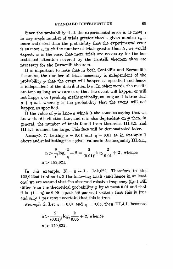
69 STANDARD DISTRIBUTIONS
Since the probability that the experimental error is at most e
in any 8ingle number of trials greater than a given number no is
more restricted than the probability that the experimental error
is at most e, in all the number of trials greater than N, we would
expect, as is the case, that more trials are necessary for the less
restricted situation covered by the Cantelli theorem than are
necessary for the Bernoulli theorem. It is important to note that in both Cantelli's and Bernoulli's
theorems, the number of trials necessary is independent of the probability p that the event will happen as specified and hence
is independent of the distributionlaw. In otherwords, the results are true as long as we are sure that the event will happen or will
not happen, or speaking mathematically, so long as it is true that
p + q ;-- 1 where q is the probability that the event will not happen as specified.
If the value of p is known which is the same as saying that we
know the distribution law, and n is also dependent on p then, in
general, the number of trials found from theorems 111.3.2. and
III.4.1. is much too large. This fact will be demonstratedlater.
Example 1. Letting e = 0.01 and - = 0.01 as in example 1
above and substitutingthese given values in the inequalityIIIA.I.,
2 2 2 2 n > -log,- + 2 -log, - + 2, whence
Z2 7) (0.01)2 0.01
n > 152,021.
In this example, N n + I 152,022. Therefore in the
152,022nd trial and all the following trials (and hence in at least
one) we are assured that the observed relative frequency (fo/n) Will
differ from the theoretical probability p by at most 0.01 and that
it is (I - 7)) = 0.99 equals 99 per cent certain that this is true
and only I per cent uncertain that this is true.
Example 2. Let e P-- 0.01 and 0.05, then III.4.1. becomes
2 2 n > - log,-_ + 2, whence(0.01)2 0.05
n > 119,832.
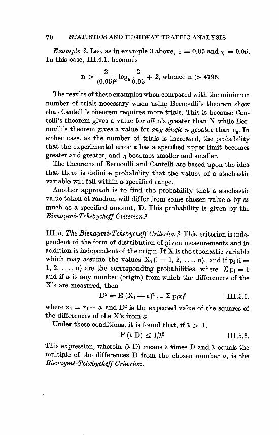
70 STATISTICS AND HIGHWAY TRAFFIC ANALYSIS
Example 3. Let, as in example 3 above, s 0.05 and 0.05.
In this case, 111.4.1. becomes
2 2 n > __ log,, - + 2, whence n > 4796.CO.05)2 0.05
The resultsof these exampleswhen compared with the minimum
number of trials necessary when using Bernoulli's theorem show
that Cantelli's theorem requires more trials. This is because Cantelli's theorem gives a value for all n's greater than N while Ber
noulli's theorem gives a value for any single n greater than no. In
either case, as the number of trials is increased, the probability
that the experimental error e has a specified upper limit becomes greater and greater, and - becomes smaller and smaller.
The theorems of Bernoulli and Cantelli are based upon the idea
that there is definite probability that the values of a stochastic variable will fall within a specified range.
Another approach is to find the probability that a stochastic value taken at random will differ from some chosen value a by as
much as a specified amount, D. This probability is given by the
Bienaymg-Tchebycheff Criterion.3
III. 5. The Bienaymg- Tcheb ycheff Criterion.3 This criterion is inde
pendent of the form of distributionof given measurements and in
addition is independentof theorigin. If X is the stochasticvariable
which may assume the values Xi (i = 1, 2, . . ., n), and if pi (i
1, 2, .. ., n) are the corresponding probabilities, where Z pi =
and if a is any number (origin) from which the differences of the
X's are measured, then
D 2 = E (Xi - a)2 = Z pX? 5. 1.
where xi xi - a and D2 is the expected value of the squares of the differences of the X's from a.
Under these conditions, it is found that, if 'X > 1,
P Q, D) ;: 1/),2 III.5.2.
This expression, wherein (X D) means X times D and X equals the
multiple of the differences D from the chosen number a, is the
Bienaymg-Tchebycheff Criterion.

71 STANDARD DISTRIBUTIONS
The criterion, to state it in words, says that the probability
P Q, D) is not more than 1/X2 that a stochastic variable taken at
random will differ from some chosen number a by as much as
?, (), > 1) times the value of D. A very useful special case is when
a is the probable or expected value.
Example 1. If the probability P (X D) <.01 and z .01, then for any a and p, X must be f FO-O IO. It will be seen later
that n must be greater than 250,000.
Example 2. If the probability P (, D) :&-.05 and e .01,
then for any a and p, ?, must be f2_0. In this case n > 50,000.
Example 3. If the probability P (X D) = - ;: .05 and s =.05,
then for any a and p, ?, must be f 2-0. In this case n > 2000.
These illustrations demonstrate that quite frequently the ex
perimenter gathers more data than is necessary for the accuracy
required. This makes the cost of the study unnecessarilylarge and
demonstrates a lack of efficiency as well as an approach that is
scientificallyunsound.
If we have a limit definition of probability, Bernoulli's theorem
is an immediate consequence thereof. In case we have any definition of probability p for the event E happening as specified, it is
possible to prove Bernoulli's theorem by the use of the Bienaym6
Tchebycheff criterion. This will be shown later in this chapter.
In general, the evaluation of the probability of a given chance
event necessitates the enumerationof all possible outcomes. These
outcomes as shown by the tossing of a penny or the drawing of a
card involve combinations and arrangements (permutations) of
happenings.
III. 6. Permutation8 and Combination& There are two basic prin
ciples in combinations:
1. If an event A can occur in a total of a ways and an event B
can occur in a total of b ways, then A and B can occur in
a + b ways, provided they cannot occur at the same time.
2. If an event A can occur in a total of a ways and an event B
can occur in a total of b ways, then A and B can occur to
gether in a - b ways.
These two principles can be generalized to take account of any
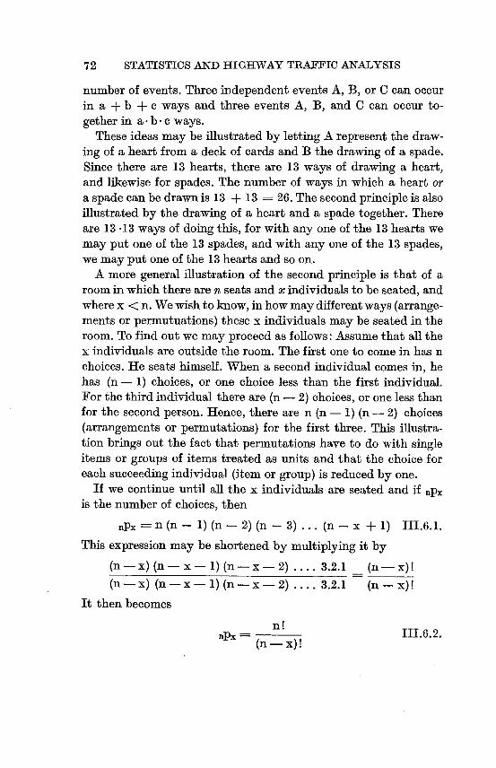
72 STATISTICS AND HIGHWAY TRAFFIC ANALYSIS
number of events. Three independent events A, B, or C can occur in a + b + c ways and three events A, B, and C can occur together in a -b -c ways.
These ideas may be illustratedby letting A represent the drawing of a heart from a deck of cards and B the drawing of a spade. Since there are 13 hearts, there are 13 ways of drawing a heart, and likewise for spades. The number of ways in which a heart or a spade can be drawnis 13 + 13 26. The second principle is also illustrated by the drawing of a heart and a spade together. There are 13 .13 ways of doing this, for with any one of the 13 hearts we may put one of the 13 spades, and with any one of the 13 spades, we may put one of the 13 hearts and so on.
A more general illustration of the second principle is that of a room in which there are n seats and x individuals to be seated, and where x < n. We wish to know, in how maydifferentways (arrangements or permutuations) these x individualsmay be seated in the room. To find out we may proceed as follows: Assume that all the x individuals are outside the room. The first one to come in has n choices. He seats himself. When a second individual comes in, he has (n - 1) choices, or one choice less than the first individual. For the third individual there are (n - 2) choices, or one less than for the second person. Hence, there are n (n - 1) (n - 2) choices (arrangements or permutations) for the first three. This illustration brings out the fact that permutationshave to do with single items or groups of items treated as units and that the choice for each succeeding individual (item or group) is reduced by one.
If we continue until all the x individuals are seated and if np" is the number of choices, then
.p. = n (n - 1) (n - 2) (n - 3) ... (n - x + 1) II1.6.1.
This expression may be shortened by multiplyingit by
(n - x) (n - x - 1) (n - x - 2) .... 3.2.1 (n - x)! (n-x) (n-x-1)(n-x-2) .... 3.2.1 (n - x)!
it then becomes
nPx III.6.2.(n - x) 1
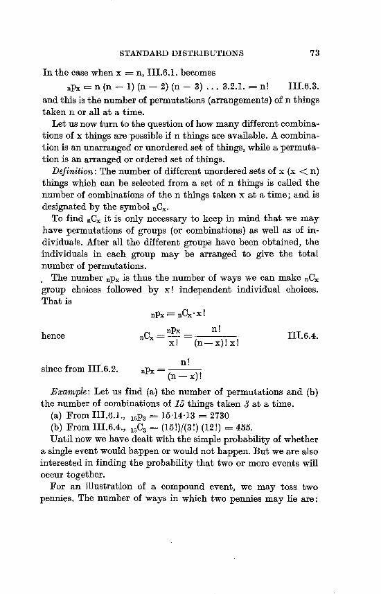
STANDARD DISTRIBUTIONS 73
In the case when x n, 111.6. 1. becomes
npx n (n - 1) (n - 2) (n - 3) ... 3.2. I. n! III.6.3.
and this is the number of permutations (arrangements) of n things
taken n or all at a time. Let us now turn to the questionof how many different combina
tions of x things are possibleif n things are available. A combina
tion is an unarranged or unordered set of things, while a permuta
tion is an arranged or ordered set of things.
Definition: The number of different unordered sets of x (x < n) things which can be selected from a set of n things is called the
number of combinations of the n things taken x at a time; and is
designated by the symbol C. To find Q, it is only necessary to keep in mind that we may
have permutations of groups (or combinations) as well as of in
dividuals. After all the different groups have been obtained, the
individuals in each group may be arranged to give the total
number of permutations.
I The number np. is thus the number of ways we can make Q,
group choices followed by x! independent individual choices.
That is
npx nCK -X!
hence CX = nPx n! III.6.4. X (n - x)! x!
since from I11.6.2. npX = n !(n - x)!
Example: Let us find (a) the number of permutations and (b)
the number of combinations of 15 things taken 3 at a time.
(a) From III.M., ILIP3 15-14-13 2730 (b) From III.6.4., 11C3 = (15!)/(3!) (12!) - 455.
Until now we have dealt with the simple probability of whether
a single event would happen or would not happen. But we are also interested in finding the probability that two or more events will
occur together.
For an illustration of a compound event, we may toss two
pennies. The number of ways in which two pennies may lie axe:
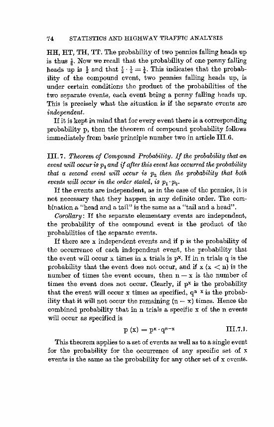
74 STATISTICS AND HIGHWAY TRAFFIC ANALYSIS
HH, HT, TR, TT. The probabilityof two pennies fallingheads up is thus 1. Now we recall that the probability of one penny falling heads up is and that I - I = 1. This indicates that the probability of the compound event, two pennies falling heads up, is under certain conditions the product of the probabilities of the two separate events, each event being a penny falling heads up. This is precisely what the situation is if the separate events are independent.
If it is keptin mindthat for every event there is a corresponding probability p, then the theorem of compound probability follows immediatelyfrom basic principle number two in article IIIA
111. 7. Theorem of Compound Probability. If the probability that an event will occur is p,. and if after this event has occurred the probability that a second event will occur is P2 then the probability that both events will occur in the order stated, is Pl'P2'
If the events are independent, as in the case of the pennies, it is not necessary that they happen in any definite order. The combination a "head and a tail" is the same as a "tail and a head".
Corollary: If the separate elementary events are independent, the probability of the compound event is the product of the probabilities of the separate events.
If there are x independent events and if p is the probability of the occurrence of each independent event, the probability that the event will occur x times in x trials is px. If in n trials q is the probability that the event does not occur, and if x (x < n) is the number of times the event occurs, then n - x is the number of times the event does not occur. Clearly, if px is the probability that the event will occur x times as specified, qn- is the probability that it will not occur the remaining (n - x) times. Hence the combined probability that in n trials a specific x of the n events will occur as specified is
p (x) = pl, -qn-x
This theorem applies to a set of events as well as to a single event for the probability for the occurrence of any specific set of x events is the same as the probability for any other set of x events.

75 STANDARD DISTRIBUTIONS
Consequently, the probability of the event's occurring exactly x times without the restriction of its being a specific x is equal to the product of the probability for any specific x occurrences by the number of combinations of x sets there are in n events. This value has been shown to be (III.6.4.) equal to
n! nCx ;-- X! (n X)!
Hence, the probability P (x) of the event's occurring exactly x times in n trials is
P (X) = . n
. pxqn-x = nC px qn-x III.7.2. x! (n - x)!
where x may assume the values 0, 1, 2, ... , n. This is a fundamental law in probability, and if we let x take on all integral values from 0 to n, we obtain the respective probability for each of the possible and mutually exclusive events.
A more general theorem in which combinations are involved is known as the Binomial Theorem.
III. 8. The Binomial Theorem (applied to probability). The Binomial Theorem states that if the probability that an action will take place in a particular way is p, and the probability that it will not be so performed is q, then the probability that it will take place in exactly n, (n - 1), (n - 2), ... 3, 2, 1, 0 out of n trials is given by the successive terms of the binomial expansion:
(p + q)n . pn + n -pn-IL q + n (n 1) pn-1 q2 . ..... 1 -2
which is known as the Binomial Distribution. It will be noted that the generating term is of the form ,Q,
P'q'. For the purpose of illustration, let a coin be tossed 3 times. In this case p =. q The probabilities of getting 0, 1, 2, or 3 heads are:
Q)3, 3 (1)3 (J)3, ffl3
and these are the successive terms of (p + q)3 p3 + 3 p1q + 3 pq! + q3

76 STATISTICS AND HIGHWAY TRAFFIC ANALYSIS
Similarly the probabilities of getting 0, 1, 2, 3, or 4 heads are:
(1)4, 4 ffl4, 6 (1)4, 4 (1)4, (1)4.
We might represent the possible results of tossing a penny four
times graphically, as shown in Figure 111.1.
6/,16
Z'
4'/I 6
2/16
0 1 2 h --------------
3 4
Number of Trials
FIGURE III. 1
GRAPHicAL REPRESENTATIONOF THE POSSIBLE RESULTS OF TOSSING A PENNY
The possibility of each number of heads is represented on the
vertical ordinate. The width of each rectangle is equal to one unit
Ax. The area of each rectangle expressed in general terms is
X, pX q- Ax 'C px qn-x
This meansthat the area of each rectangle equalsthe probability
of getting the number of heads corresponding with the mid-point
of its base. The entire area . the probability of getting 0, 1, 2, 3,
or 4 heads = I 1 4 + 6 + -I- + I = 1, so that the prob16 ' If, 16 16 16 ability of getting a given number of heads is equal to
Area of rectangle
Area of whole figure
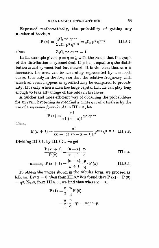
77 STANDARD DISTRIBUTIONS
Expressed mathematically, the probability of getting any
number of heads, x Cx px qn-x
P (X) = ' = nCX pX qn III.8.2. I C px qn-x
since ZnCx px qn-x
In the example given p = q = with the result that the graph
of the distribution is symmetrical. If p is not equal to q the distri
bution is not symmetrical but skewed. It is also clear that as n is
increased, the area can be accurately represented by a smooth
curve. It is only in the long run that the relative frequency with which an event happens as specified may be compared to probab
ility. It is only when a man has large capital that he can play long
enough to take advantage of the odds in his favor. A quicker and more efficient way of obtaining the probabilities
for an event happening as specified x times out of n trials is by the
use of a recursionformula. As in Ill. 8.2., let
n ! P (x) px qn-x
x! (n - x)!
Then,
n! P (x + 1) = (x + 1)! (n px+1 qn-1 III.8.3.
Dividing 111.8.3. by I11.8.2., we get
P (x + 1) (n-x) P
P (X) x + 1 q
(n - x) pwhence, P (x + 1) P (X) III.8.5.
x + q
To obtain the values shown in the tabular form, we proceed as follows: Let x = 0, then from III. 8.2 it is found that P (x) = P (0)
qn. Next, from III.8.5., we find that where x = 0,
P (1) PP (0) q
p- qn = nq n-1 P.

78 STATISTICS AND HIGHWAY TRAFFIC AXALYSIS
Then, let x = I in III.8.5., and
n-1 PP (2) - .- P (1)
2 q
n-I p . nqn 2 q
1) qn-2 2 2! p
Continuingin this way, all the probabilitiesof happenings may be
obtained and they are shown in the followingtable for the different
possibilities.
Table III. 1
BiNomiAL DisTiuBUTION
Number of Probability of Happenings Happenings
0 .................... qla
I .................... nq"-' p n(n-1) _2 2
21 . qr,
3 .................... 1) (n3
2) q-$ p3
.................... .
..... I.... I......... .
.................... .
.................... nTI(. )! q11 p,
.......... I......... .
.................... .
.................... .
n .................... P n
Such a description of happenings is designated a probability
distribution or a relative frequency distribution in the case of a
sample. If each of the probabilities were multipliedby the number
of individuals (number of cases or number of trials), we would have
the corresponding theoretical (absolute) frequency distribution.
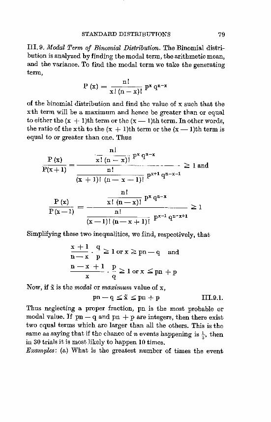
79 STANDARD DISTRIBUTIONS
III. 9. Modal Term of Binomial Distribution. The Binomial distribution is analyzed by finding the modal term, the arithmetic mean,
and the variance. To find the modal term we take the generating
term,
nP (X) px qn-x
x! (n - x)!
of the binomial distribution and find the value of x such that the
xth term will be a maximum and hence be greater than or equal
to either the (x + I)th term or the (x - I)th term. In otherwords,
the ratio of the x th to the (x + I)th term or the (x - 1)th term is
equal to or greater than one. Thus
n! ... px qn
(X) (n I and
P(x + 1) n PX+1 qn-x-I
(X + (n - X
n !
P (X) X! (n X)! px qnX
PK-' qn-x+l (x - 1)! (n - x + 1)!
Simplifying these two inequalities, we find, respectively, that
x + q - : I or x . pn - q and
n-x p
n-x + I p :- lorx <pn +p x q
Now, if R is the modal or maximum value of x,
pn - q : i : pn + p III. 9. I.
Thus neglecting a proper fraction, pia is the most probable or
modal value. If pn - q and pn + p are integers, then there exist two equal terms which are larger than all the others. This is the
same as saying that if the chance of n eventshappening is ' 3)
then
in 30 trials it is most likely to happen 10 times.
Examples: (a) What is the greatest number of times the event

80 STATISTICS AND HIGHWAY TRAFFIC ANALYSIS
will happen as specified when there are n 11 trials and when p = q I From III.9.1., we find that i is either 5 or 6.
2 '
(b) If n 12 trials and p q :i 6.2
(c) If n = 15 trials and p 6
and q P :i 2.
(d) If n = 18 trials and p ' and q ',:i 3.6 6
(e) If n = 23 trials and p 'andq' :i3orC6 6 2
III. IO. Arithmetic Mean of Binomial Distribution. Let _X be thearithmetic mean (mathenzatical expectation - probableor expected number of times the event will happen as specifiedin n trials under thelaw of repeated trials). By definition, the arithmetic _X of x is
n
'Y' X px qn-x
0 (n -- x) 1 n I III. IO. 1.
- px qn-x Ex X! (n x)!0
But the denominatoris the total probability which is equal to 1. Simplifying,
n (n - 1)x O-qn + I -nqn-lp + 2 - qn-2 p2 +
21
= np (q--l + (n - 1) qn-2p + (n 1) (n 2) n-3 2 2 q p
np (q + p)n-I = np np. III. 10. 2.
Illustrative Example 1: Given p and n 18, and q 16 6
required to find the mean _x. Substituting in 111.10.2,
X = 18 3. 6
The answer may be interpretedto mean that in the long run the event will happen one time in 6 trials and therefore in 18 trials we would expect the number of occurrences to be 3, while the actual riumber of occurrencesin a single trial may be x = 0, 1, 2, 32 ... ,18,
Illustrative Example 2: Suppose that it has been ascertained from a traffic count that on the average 30 per cent of the vehicles turn
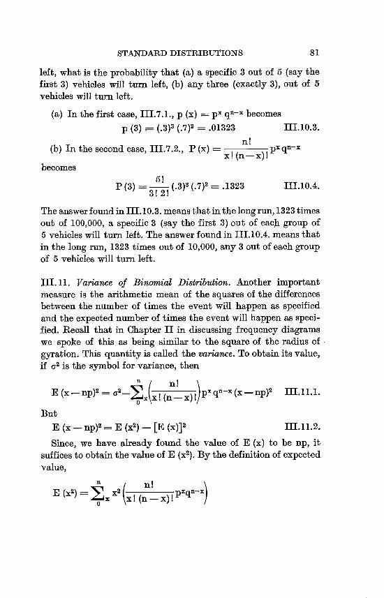
81 STANDARD DISTRIBUTIONS
left, what is the probability that (a) a specific 3 out of 5 (say the
first 3) vehicles will turn left, (b) any three (exactly 3), out of 5
vehicles will turn left.
(a) In the first case, III.7. I., p (x) = px q-x becomes
p (3) ;-- (.3)3 (.7)2 =.01323 III. 10.3.
n! (b) In the second case, III.7.2., P (x) px qn-x
X! (n - x)!
becomes
P (3) (.3)3 (.7)2 .1323 III.10.4. 3! 2!
The answerfound in III. 10.3. means that in the longrun, 1323 times
out of 100,000, a specific 3 (say the first 3) out of each group of
5 vehicles will turn left. The answer found in III. 10.4. means that
in the long run, 1323 times out of 10,000, any 3 out of each group of 5 vehicles will turn left.
III. II. Variance of Binomial Di8tribution. Another important measure is the arithmetic mean of the squares of the differences between the number of times the event will happen as specified
and the expected number of times the event will happen as specified. Recall that in Chapter 11 in discussing frequency diagrams
we spoke of this as being similar to the square of the radius of
gyration. This quantity is called the variance. To obtain its value,
if G2 is the symbol for variance, then
E (X _ np)2 G2 E.n t
I px qll-x (X - np)2 III.
0
But
E (X - np)2 E (x2) - [E (x)]' III. I 1.2.
Since, we have already found the value of E (x) to be np, it
suffices to obtain the value of E (x2). By the definition of expected
value,
n E (x2) ;" . X2 pxqn
0 x! (n-x) I X)

82 STATISTICS AND HIGHWAY TRAFFIC ANALYSIS
O.qn + Lnqn-lp + 4 n (n- 1) qn-2P2 2!
+ 9 n (n- 1) (n- 2) qn-p3 ................ 31
np q-nl+2(n-l)q-2p+ 3(n-1)(n-2) q-3p2 + 1 2 !
np (q + p)n-1 + (n- 1) p I qn-2 + (n - 2) qn-3 p
+ (n 2) (n 3) qn-4 2 . .............. 2 ! p
np + (n - (p) (q + p)n-2]
np + (n - p] = np + n2 p2 - np2
Substituting the values from III.11.3. and III.10.2 in III.11.2., we find
a2 = E (x - np)2 = E (x2) - [E (X)]2 becomes 01 = np + n2 p2 _ np2 n2 pl
= np - np2 = np (I - p) = npq III.11.4.
Illu8trative example: Given p 1,6 q 1,6 and n 18. From
III.11.4. we find that a2 = 18 2.5. This means that in6 6 18 trials we would expect the number of occurrences to differ from
3 by 2.5. In other words, we would expect the actual number of
occurrences to lie between 3 - 2.5 0.5 and 3 + 2.5 = 5.5, namely, between 1 and 5.
In the case of relative frequency or relative number of occur
rences, if (x/n - p) is the difference between the observed number
of occurrences out of n and the probability p of occurrence, then it is not hard to show that
E (X/n - p)2 - E (X _ np)2 G2 pq III. 5.
n2 n2 n
III. 12. Size of Sample Required for Stability. At this point it should
be noted that we are thinking of the relative frequencies in many
random samples, and that we are concerned about the degree of

83 STANDARD DISTRIBUTIONS
stability or the degree of dispersion of such a series of relative
frequencies. This is a fundamental problem in statistics. In the binomial distribution, sometimes called the Bernoulli distribution
we assume that the underlying probabilityremains constant from
trial to trial and from sample to sample and that the drawings are
mutually independent. This assumption is implied in so-called ,simple sampling.
RetumingtoBernoulli'stheorem,III.3.1.,Iet e?, Eq, (?, > 1).Yn
In the Bienaym6-Tchebyeheff inequality, III.5.2., let D = Yjn_.
Then
P Q, D) becomes P (e) < pq III.12.1 X2 n e2
It may be seen from 111. 12. 1. that as n tends to infinity, I = P (s) tends toward zero. This proves Bernoulli's theorem for any dis
tribution law of probability by the use of Bienaym6-Tchebyeheff
criterion as was suggested in 111.5.
In order to get a comparison of the results obtained by articles
III.3., IIIA., III.5., let e = 0.01, p 0.1, q 0.9, X = 2 Y-5
4.472 and 0.05. Substituting these values in III.12.1.,
pq P (e) jje2
P (.01) 0.05 P) (.9) n (.01)2
whence n I,-- 18, 0 0 0.
Again let e 0.05, p 0.1, q = 0.9, X 2 Y5 4.472 and
0.05. Substituting these values in 111.12.1., we get
P (P-) < pqne2
P (.05) 0.05 < (J) (.9) n (.05)2
whence n '-> 718.
Comparing these results with those previously found, it is seen
that they are materially less as was indicated previously. It is

84 STATISTICS AND HIGHWAY TRAFFIC ANALYSIS
noted that n is a maximum when p = q for then pq is the maximum. Hence, it is always safe to take the value of n when p and q equal as the minimum value of n. That is, in case the values of p and q are not known, it is safe to use p = q I in determiningthe size of sample required. In many traffic problems, p is very small and q very near unity which will require a smaller sample for stability than if p were equal or nearly equal to q.
Additional means of characterizing the binomial distribution are moments about the mean. These are:
0
IL2= npqtZ3= npq (q - p)k= 3 p 2q2 n2- pqn (I - 6 pq) III. 12.2...................................
[LX ;--= (j - np)x qn-j pJ0 [tx+l pq nx[tx-l +
dp,
where is the number of combinations of n things taken at a
time and n is very large. Other characterizingmeans are the P coefficients:
(q - p)2
npq
P2 3 + I - 6 pq III. 12.3. npq
PI is a coefficientof skewness, while P2 is a coefficient of kurtosis or "peakedness".
The theorems of Bernoulli and Cantelli and the Bienaym6Tchebycheff criterion are devoted to obtaining a lower limit to the probability that the experimental error will not exceed a given amount.
The binomial distribution and particularly its generating function P (x) given in III.7.2. gives the actual probability of the
85 STANDARD DISTRIBUTIONS
event's occurring exactly x times in n trials, so that it is possible
to determine the actual probability of the event's occurring between any two specified number of times in n trials. This is ac
complished by adding the respective separate probabilities in
volved since the events are mutually exclusive.
The function P (x) is given by
P (x) n x)! pxqn-x
The function P (x) is a fundamental law of probability for all
positive values of x, integral or fractional. The function is con
tinuous almost everywhere (i. e. except for negative integers) and
has a unique value for every positivevalue of x. It is simple enough
to handleif x is an integer. It is quite difficult an& cumbersomeif
x is not a positive integer. In practice it is most usable when x is a whole number. Many
times, however, x is not a whole number. It then becomes im
perative, if possible, to derive from the function given in III.7.2.
another continuous function which is easier to use and also gives us the actual probabilities (not lower limits only) that are desired
to be known. Two such functions are the Normal Distribution and the Poi88on
Distribution. We shall now develop and discuss these two func
tions.
III. 13. The Normal Distribution. The normal distribution is a con
tinuous approximationto the binomial distributionwhenn is large
and p and q are not small.
Let us reexamine the generatingterm P (x) of the binomial dis
tribution, namely,
n! P (X) pxqn-x III. 13. 1.
x! (n - x)!
The graph of this equationis a set of points whose abscissas are x
values and ordinates are the corresponding P (x) values for all
values of x from zero to plus infinity. The function P (x) is con
tinous almost everywhere (i. e., except for negative integers).
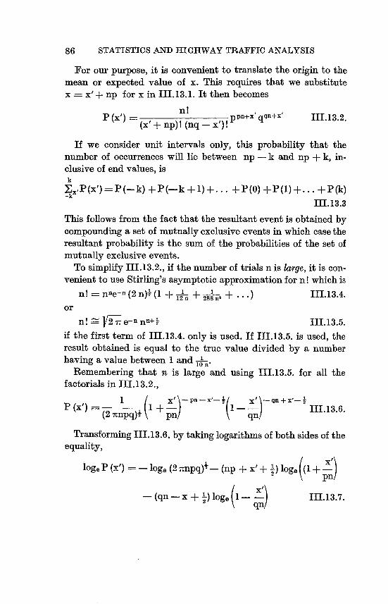
86 STATISTICS AND HIGHWAY TRAFFIC ANALYSIS
For our purpose, it is convenient to translate the origin to the mean or expected value of X. This requires that we substitute x XI+ np for x in III. 13. I. It then becomes
n! I P (XI) = (XI+ np)! (nq - XI)! PPn+X qqn+x' III.13.2.
If we consider unit intervals only, this probability that the number of occurrences will lie between np, - k and np + k, inclusive of end values, is k
kX P(x')P(-k)+P(-k+1)+... +P(O)+P(I)+...+P(k) III. 13.3
This follows from the fact that the resultant event is obtained by compoundinga set of mutually exclusive events in which case the resultant probability is the sum of the probabilities of the set of mutually exclusive events.
To simplify 111.13.2., if the number of trials n is large, it is convenientto use Stirling's asymptotic approximationfor n! which is
n! nne-a (2 n)y' (I + 121 n + 288 ' n' + III. 13.4. or
n! V-27 e-n nn+'2 III.13.5.
if the first term of III. 13.4. only is used. If III. 13.5. is used, the result obtained is equal to the true value divided by a number having a value between 1 and 101n.
Remembering that n is large and using 111.13.5. for all the factorials in 11I.13.2.,
P (XI) XI pn -x'- 'T(I XI -qn+x'-vl
III. 13.6. (2 7rnpq)' P qn)
TransformingIII. 13.6. by taking logarithmsof both sides of the equality,
XI loge P (XI) log (2 -npq)'2 - (np + XI + 1) log,, +
5 2 pn)
(qn - x + 1) log. I - XI III. 13.7. 2

87 STANDARD DISTRIBUTIONS
xi Expanding log,, I + X' and log, I - - in power series of x',
pn) qn) 111.13.7. becomes
log. [P (x')] [27cnpq]i (np + x, + t) r x' x'2 R (x')[np inij n3
X12 Xf3
- (qn - x'+ 1) x S (X') III.13.8. 2 L-q- 2 n2q n3 I
To make this expansion valid, it is necessary to assume that n
is sufficiently large so that x-' 'is sufficiently small. It follows that n
R (x') and S (x') are finite. Simplifying III.13.8., and performing the multiplying opera
tions indicated, we find that I
(p - q) x' x12 xf2 T (x') III. 13.9. log, [P (x')] [27cnpq]l= 2 npq 2 npq + 2
The equation 111. 13.9. may be written in the form X12 Xf U
10& [P (x')] [2 nnpq]I= - - - III. 13. 1 0. 2 npq n
where U (x') is also finite. Now if n is large enough (in other words, n must be very large)
xi so that - U (x') is very small (negligible or within the allow
(n) able error), then ignoring this term, III.13.10. may be written as
I _X'. P (X') = F2 _ n-p_q)fe2 npq III. 13. 1 1.
which is called the normal distribution. It appears that this was first known to DeMoivre in November,
1732. Multiply both sides of the equality H1.13.3. by Ax', then, k
Z,,, P (x') Ax' P (- k) Ax'+ P (- k + 1) Ax. . ..... + P (0) Ax' k
+ P (1) Ax'+ P (k) Ax' and on the assumptionthat P (x') is continuous,
k 1 k XI,
Lim e - 'f'-Pqdx' III. 13.12. Ax,-->. OE-,p (x') Ax'F-- _271npq)` fk

88 STATISTICS AND HIGHWAY TRAFFIC ANALYSIS
The right hand memberof III. 13.12 is known as the probability
integral. It gives the probability that a random variable x'has the
value - k : x':: k. If P (x') is discontinuousand the ordinates are at unit intervals,
then in III. 13.3. there is one more ordinate than intervals of area.
Hence, k+
k I
-k P (X')
F2 q),-e2_nPqdx' approximately. III. 13.13._;np x"
The above resultssummarizedlead to the well-known DeMoivre-
Laplace theorem, namely": The probability that the difference x' x - np between the
number of occurrences x and ae, expected number of occurrences will
not exceed a positive number k is given to a first approximation by
111.13.12 and to closer approximation by 111.13.13.
III. 14. Interpretation of ae Properties of Normal Distribution. The
special form of the normal distributionas given in III. 13. 1 1. is re
stricted to the conditions that n is large and p and q are not small
thus giving a continuous approximation to the binomial distri
bution.
1 -72
Now consider P (x) e 20 III. 14. 1. 2
where a is the standard deviation with the restriction that it is
finite such that 0 _- cr : k.
The graph of the equation is shown in Figure III.2.
From III. 14. 1., it is seen that the curve is symmetrical with
respect to the y-axis. Likewise the curve has a maximum point at
x = 0, namely at the point whose abscissa is the arithmetic mean.
There are two points of inflection, namely P, and P2 each of which
are at a distance a from the arithmetic mean. The curve is asymp
totic to the x-axis at both plus and minus infinity.
From III. 14. I. or from tables, it is found that the total area
under the curve is unity, the area between x - a and x + a

STANDARD DISTRIBUTIONS 89
is 0.6827, the area between x 2 cr and x + 2 cr is 0.9545,
and the area between x ;== - 3 a and x + 3 a is 0.9973. If
2 fx - x' I
a V2 7c 0e -i -0 dx 2
then x ;== 0.67449 a III.14.2.
which is known as the probable error.
YY=P(X)
4
3
pi P2
a. x36- 26- a- 6' 26- 36
FIGURE III.2
1 - Xs
GRAPH OF THE EQUATION P (X) 2 7C e 20
As an illustration, consider again the case 0.05, e ="0.01.
From the Bienaym6-Tchebycheffinequality, A t 4.472. Now,
let p = q L. Then, from 111. I 1. 5. and Ill. 12. L,2 trp-qi e
n
becomes 4.472 1 M) m :: 0.01V n whence n : 500
Similarly, if - 0.05 and e == 0.05

90 STATISTICS AND HIGHWAY TRAFFIC ANALYSIS
pqt -:< z Vn
becomes 4.472 (Y'01) :< 0.05 V n
whence n '-> 100.
Again, let p and e 0.01. The value of t such that
2 t 2
- e 2 dX . 0.99 = I
V2 7c t
is 2.58. But n pqt'. Hence, solvingfor n, it is found that n 166 2
and if
2 t Xi
r271 f e 2dx=0.95=1--n, _t
t = 1.96 and n --> 97, if s = 0.01.
Under certain conditions where p q, the equation of the continuous approximationcurve is given by
NpP+1 +?E)ya y = aep r (p + i) e a 111.14.3.
where the origin is at the mode. The question is often raised: How is it known that the distribu
tion is normal? A very good answer is: If it can be justified axiomatically that the arithmeticmeanis the most probablevalue, then the distribution is normal. This is known as the postulate of the arithmetic mean. Another way is: If p, 0 and P2 = 3 (See II.25.17. and 11.25.18.), the distribution is normal.
III. 15. PoissonDistribution. This distributionis frequentlythought of as the law of small probabilities or the law of rare events. It appears to be especially useful in solving many traffic problems (see Chap. V).

STANDARD DISTRIBUTIONS 91
Consider again the generating term of the binomial expansion,
n! P (X) = 1(n X) , pxqn-x III.15.1.
the probability that in n trials exactly x of them will take place as
specified, where p is the probability that the event in a single trial will occur as specified.
Equation II1.15.1. may be written as
P (X) 1) 2) (n + 1) PK (I - P)n-x x
111.15.2.
M Write p - where m is the number of times a given happening
n
occurs in n trials. Substitutingthis value of p for p in III. 15.2.,
(n) 'n - 1) (n - 2) (n-x +I /mx )U(,-M -X P (X) = I _M
n n n X!)( n n)
III. 15.3.
Now, hold both x and m fixed and let n approachinfinity. Then, in the limit,
n n - 1 n-x +I M -X -= 1) - = II ....... = 1, and I 1. n n n n)
M n To obtain thelimiting value of (I - n) we set
II1.15.4. Mn)n = [(1 - vnr] M
M ni
The limiting value of I - - as n approaches n)-1
infinity is e-1. Hence ) i,
Lim -M ]% e- M. 111.15.5. n-00 n
Substituting all the limiting values just found in 111.15.2., we
obtain MX
P (x) (1) - e-m. (1) III.15.6. x

92 STATISTICS AND HIGHWAY TRAFFIC ANALYSIS
which may be written as
mx e-m P (X) I 11I.15.7.
which is Poisson's distribution or the Poi88on Exponential Func
tion. This function is a continuous approximation to the binomial
distributionwhen p is small and n is large.
The function is continuous almost everywhere and has a real
value for all values of x except negative integers. For negative
integral values of x, P (x) is not defined. The continuityis obvious
if it is recalled that x! is related to the Gamma Function,9 that is:
X! 0 y X e-y dy = U1.15.8.r (X+1) The graph of the functionis shown in Figure I11.3. Also tables
(Tables for Biometricians and Statisticians, pp. 122-124) of values
for Px exist.
5' P 0 5 -1 E JW.
A E
rn=l.o
3
2.0
2
-M-10.0
2 4 6 8 10 12 14 16 18 20
Valm of X
FIGur.E III.3 RIX e-M
GRAPH OF THE FuNcTioN P (X)

STANDARD DISTRIBUTIONS 93
From the figure it is seen that for Small values of m the curve is
highly skewed and that as the values of m increase the curve be
comes more symmetrical. In all cases, p must be small and n must be large, but small
values of m as well as large values of m are possible under these
conditions. It is also quite important to note that as M becomes
larger, the agreement between III.15.7. and III.13.11. becomes
closer.
III. 16. The Sum of the Term8 of the Poimon Di8tribution. Since each
termis theprobabilityfor the event's happeningx times, the sum of
the probabilities for each of these possibilities should equal unity
because some one of the possibilitiesis certain to take place. Letting
x take successively the values 0, 1, 2, the sum of the re
spective terms is
Go mx e-m MO e7m me-M M2e-M
0 x X! 0! 21
M M2 M3 e_m(l +_+_+_ + III. 16. 1.
I ! 2 ! 3 !
The series in parentheses has the value e'. Hence
m'e-M X! e-mem = eO= III.16.2.
III. 17. The Arithmetic Mean of Poi8son Di8tribution. If _x is the
arithmetic mean number of happenings, then
co mle7-- M x EX0 X!x
Moe` me-M m2e-m In3e-M. - I + - 2 + - 3
0 + 1 2 ! 3
M M2 M3
= me-m I +T! +- +- +...1 2 3
= me-meM = M.

94 STATISTICS AND HIGHWAY TRAFFIC ANALYSIS
III. 18. Phe Variance of Poimon Distribution. Since variance is the
expected value of the squares of the measurements minus the
square of the expected value of the measurements, we will first
obtain the expected value of the squares of the measurements. It
is given by,
W mx e- in (X2) ). X2
0
Moe` me-m m2e-' m3e7m __0 0 + - 1 ! I + - 2 1 4 + - 31 9 . .....
+ 2 m 3 m .. . .] ][n e- __ + - +
1! 2!
e7. [6m + ( M2 M3 +M In +
me-1n [em + m m m . .....I ! 21
me-m [em + me- ];== m + m2 111.18.1.
But the square of the expected value is M2. Hence
a' E (xl) - [E (x)11
in + M2 - M2 M 111.18.2.
Example 1. There occurred at a certain highway intersection 6
accidents during the passing of 10,000 vehicles. In this case p =
0.0006 and n 10000. Suppose we wish to know the probability
that the number of accidents lies between 3 and 9 per 10000 ve
hicles. Making use of 111.13.13., we find that
k+j 31 XI' - 'IS
P (x) ell.9928 dX'=: 0.02654 efl-.-9928 CIX' (27cnpq) 1E _k-j 3
From tables of the normal probability function it is found that if
xfl 3.5 z - = 1.429
2.449
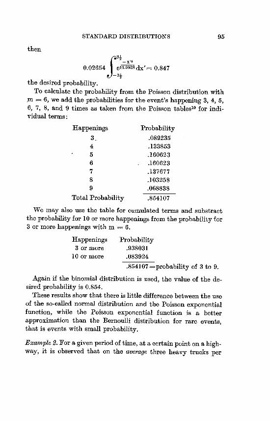
STANDARD DISTRIBUTIONS 95
then
0.02654 ell.9928 dX'= 0.847
the desired probability.
To calculate the probability from the Poisson distribution with
6, we add the probabilities for the event's happening 3, 4, 5,
6, 7, 8, and 9 times as taken from the Poisson tables10 for indi
vidual terms:
Happenings Probability
3- .089235
4 .133853
5 .160623
6 .160623
7 .137677
8 .103258
9 .068838
Total Probability .854107
We may also use the table for cumulated terms and substract
the probabilityfor 10 or more happeningsfrom the probabilityfor 3 or more happenings with m 6.
Happenings Probability
3 or more .938031
10 or more .083924
.854107 probability of 3 to 9.
Again if the binomial distribution is used, the value of the de
sired probability is 0.854. These results show that there is little difference between the use
of the so-called normal distribution and the Poisson exponential
function, while the Poisson exponential function is a better
approximation than the Bernoulli distribution for rare events,
that is events with small probability.
Example 2. For a given period of time, at a certain point on a high
way, it is observed that on the average three heavy trucks per

96 STATISTICS AND HIGHWAY TRAFFIC ANALYSIS
100 vehicles pass the point. A subsequent sample contains six
heavy trucks per 100 vehicles. Using the Poisson exponential dis
tribution, compute the probabilities of 0, 1, 2, 3, 4, 5, 6, 7, and 8
heavy trucks per 100 vehicles using m = np = 3.
The probability distributionis shown in Table III.2.
Table III.2.
X PX X PX 0 .0498 5 .1008 1 .1494 6 .0504 2 .2240 7 .0216 3 .2240 8 .0081 4 .1680
This table shows that (1) the probability of obtainingone heavy
truck in a sample of 100 vehicles is 0.1494; (2) the probability of
getting more than three heavy trucks is .5768; (3) the probability
of getting at least six heavy trucks is .3080.
The probability of six or less than six, being .9664 with a level
of significance of I - .9664 .0336, indicates that on a 5 percent
level we have grounds to reject the hypothesis that this number
of heavy trucks is not significant.
In obtaining the size of the sample so that the error from the
arithmetic mean is one heavy truck, namely, that the number of
heavy trucks is between 2 and 4, the reasoning is:
The standard deviation is
a m = np n (.03)
and since e = 1, it is clear that
e tM
becomes I (1/3) n (.03)
which gives n P-_ 100
and the sum of the probabilities, namely
-2240 + .2240 + .1680 = .6160, the measure of certainty.
Example 3. Required to find the probability of n cars appearing
within an interval of time r beginning at the instant, t. Then
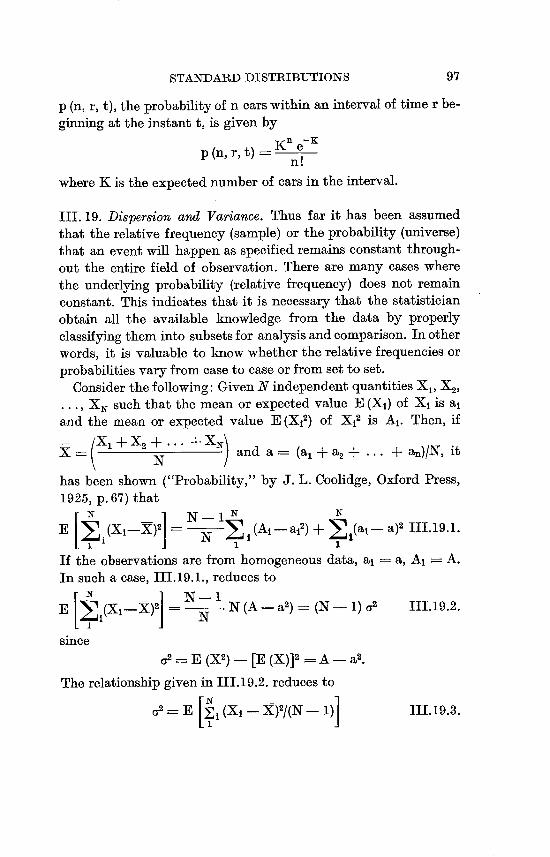
STANDARD DISTRIBUTIONS 97
p (n, r, t), the probabilityof n cars within an interval of time r be
ginning at the instant t, is given by
p (n, r, t) =K" en!
where K is the expected number of cars in the interval.
III. 19. Dispersion and Variance. Thus far it has been assumed
that the relative frequency (sample) or the probability (universe)
that an event will happen as specified remains constant through
out the entire field of observation. There are many cases where
the underlying probability (relative frequency) does not remain
constant. This indicates that it is necessary that the statistician
obtain all the available knowledge from the data by properly
classifying them into subsets for analysis and comparison. In other
words, it is valuable to know whether the relative frequencies or
probabilities vary from case to case or from set to set.
Consider the following: Given N independent quantitiesX,., X21
... I XN such that the mean or expected value E (Xi) of Xi is aj
and the mean or expected value E (X?) of X? is Ai. Then, if
- = (XI + X2 + - - -+XN X N ) and a = (a,, + a, + + a.)/N, it
has been shown ("Probability," by J. L. Coolidge, Oxford Press, 1925,p.67)that
N N - I N N E (Xi-X)2 - N Y, I (Al - a?) + Y (a, - a)2 III. I 9. 1.
If the observations are from homogeneous data, a, a, Al A. In such a case, III.19.1., reduces to
N N - 1 E (Xi-X)2] = N .N (A - a) = (N - 1) c72 III.19.2.
since
a2 = E (X2) - [E (X)]2 A - a2.
The relationshipgiven in III. 19.2. reduces to
[NC72 = E 5,, (Xi - X)2/(N III. 19.3.
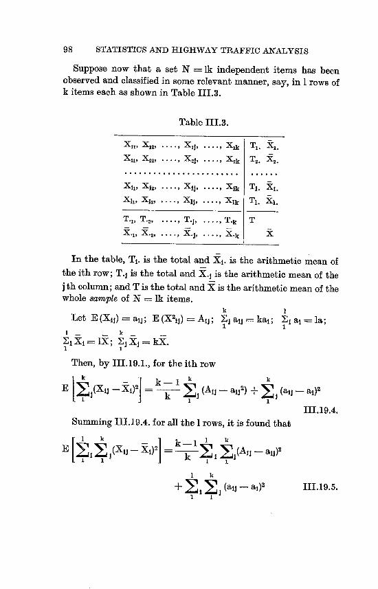
98 STATISTICS AND HIGHWAY TRAFFIC ANALYSIS
Suppose now that a set N = lk independent items has been observed and classified in some relevant manner, say, in 1rows of k items each as shown in Table III.3.
Table III. 3.
xnl X12, -, XiJ. ..... XjLk TI. St,
X21, X2V .... I XJ . ..... Xk T, j':2.
. . . . . . . . . . . . . . . . . . . . . . . .. . . . . .
XIV Xh .... PXlj' .... P x1k T1 - Xi.
Xh, X12. ..... Xlj, - - --, 'Xlk Tl- Rl.
T.1, ..... T.j . ..... T-k TT-2 s
:R.21 X-J,
In the table, T1. is the total and Xi. is the arithmetic mean of
the ith row; T.j is the total and X.j is the arithmetic mean of the
j th column; and T is the total and X is the arithmetic mean of the whole sample of N = lk items.
k Let E (Xjj) = aij; E (X2,J) A1j; 1j aij = kal; El at = la;
k El Xi IX; EJ Xj = kX.
Then, by III. 19. I., for the ith row
k k - I k k E EJ (Xii -Xi) - EJ (Aij - alJ 2) + EJ (aij - aj)2
k
III.19.4.
Summing 111.19.4. for all the I rows, it is found that
I k k-1 I k[)jl E,(Xjj - 1)2
-El EI(Alj - alj )2
L k- I I
I k J(aij - al)2

99 STANDARD DISTRIBUTIONS
Since E (Xi.);== a,, we note that
E (Xi. - a,)' E (Ki.1) - 2 at E (XI.) + a? E (X1.2) a? or
E (XI.2) E (Xi. - a, )2 + a? III.19.6.
Applying III. 19. 1. to Xi. (i 1, 2, . .
Xi. [E i a (atK)2 )2(X2.) 1]
III.19.7. But
k E a! E (Xi. - al)2 J (Aij - aij)
k2
so that
ElI - 1-1 I kE (Xi.-K)2 Ej(Ajj-ajj)2 (at - a)2 2
III.19.8. Applying III.19.i. to the Nlk values, we get
E[ I Ik(Xjj - 5)2 lk-I ' k Y -Elk 1
1 k EJ (aij - a)2 III.19.9.
By starting with the j th column and proceeding as in III. 19.5., III. i 9.6., an III. 19.7., it is found that
[ k - =1_1 k IE E JE I(XIJ - X.J)2] - Ejy ,(Ajj - 0j)
k I
+ E , (aij - bj)2 III. 19. 1 0.
and [ k -)21=k- I k I k
E E X - 'F, J'Y,, (Aij - 01j) + EJ (bj - a)2k12
19.1 1.

100 STATISTICS AND III GHWAY TRAFFIC ANALYSIS
If the N = lk values are statistically homogeneous or are all
observations from the same population, then Ali A, aij = a,
= bi = a so that III. 19.5., III. 19.8., III. 19.9., and III.19. 1O.,
and III.19.11., become, respectively I k k-1
E k .lk (A - a2) I (k - 1) (A - a2)11EI(Xii-Xi.) III.19.12.
X - YQ2] lk2 lk (A-a 2) (A - a2) III. 19.13.
E[ I I k (XIJ - _)2 lk- 1 2) Y 'Y' X - - lk (A- a);:-- (1k - 1) (A- alk
III.19.14.
E[EJEI(X'J_' J)2 lk (A - a2) k(1-1)(Aa2)
III. 19.15. k k_1
lk (A - a) - (A - a2) III. 19.16.
To summarize, it has been shown that in a statistically homo
geneous set of N = lk observations arranged in I rows and k columns, the following estimates of variance (or the following
mean sums of squares) all have the same expected value: I k - I k
'F., 11 (XIj X)2 5"i EJ (XIj - Xj.)2
(2)lk - 1 1 (k - 1)
III. 19.17. k I 7,J El (XIJ - X.J)2 k Z, (XI. - X)2
(3) .' - (4)k (I - 1)
k
Ili (X-J -X)' (5) 1
k-I
Any significant differences between the estimates given in
III.19.17. indicate lack of homogeneity of the set of items. The tests for this will be described in Chapter IV.

STANDARD DISTRIBUTIONS 101
Let us now consider several special cases. Let plj be the prob
ability that X has the value Xlj andlet pibe the average probability
for the ith set, then
k kpi EJ Pij; lp = El pi
1 1and it can be shown by the use of III.19.1. thatI k I k
El EJ (Xlj - X)l = lkpq- El EJ (plj - pi)' + (k2 - k) El (pi - p)2
III.19.18.
The special cases are:
(1) Bernoulli series: pij pi p. Here III. 19.18 becomes I k
EiE (Xij- X)2 1kpq1 ii
(2) Lexis series: pij pi; pi --- p. Here III.19.18. becomes_T_ I k
It EJ (Xjj - X)l lkpq + (kl - k) El (pi - p)2. 1 1 1
(3) Poisson series: pij =_=F pi; pi =_ p. Here III. 19.18. becomesI k I k
El EJ (Xlj - X)l lkpq- 11 EJ (pj - p)2 I 1 1 1
The special cases expressed verbally are:
(1) Bernoulli series: The underlying probabilityp is constant from
trial to trial and set to set or is constant throughout the whole
field of observation and we have statisticalhomogeneity.
(2) Lexis series: The probability is constant from trial to trial
within a set but varies from set to set and we do not have sta
tistical homogeneity.
(3) Pois8on series: The probabilityvaries from trial to trial within
a set of k trials, but the several probabilities for one set of k trials
are identical to those of every other of 1 sets of k trials and we do
not have homogeneity.
Illustrationsof such series exist in the study of traffic on a given
route at I different crossings at k different times with a total of N = lk observations.

102 STATISTICS AND HIGHWAY TRAFFIC ANALYSIS
III. 20. The Multinomial Di8tribution: Let samples of size n be
drawn from a specified universe with each sample divided into
the k classes or cells with the distribution random among these
classes or cells. The probability,P, that there are f., individuals in the first cell,
fO2 in the second cell, and so forth, is
P = 7CIfOl 7rfO2 . . . . . 7C,,fbk n I11.20.1.
fOl ! fO2 !..... fOk !
where 7r, is the probabilitythat an individual falls in the first class
or cell, 7c2 the probability that it falls in the second cell, and so
forth; and
n!
f1l ! fO2 !. . . . .f0k!
is the number of combinations of n things taken for. of one kind,
f12 of another kind, fOk of the k-th kind.
To illustrate: At an intersection point it has been determined
that the probabilityof turning left is 2 of going straight ahead is 5 )
and of turning right is 1 0 Of 6 vehicles, what is the probability
that one will turn left, two will go straight ahead, and 3 will turn
right ?
Solution: Here 7r, 2 0.4, 7c2 = I = 0. 5, and 7r3 0. 1. 5 2 1 0
Also fol = 1 1 fO2 2, fo', 3. Substituting these values in M. 20. I.,
P = (0.4)1 (0.5)2 (0.1)3 ! 1! 2! 3!
0.0001 (60) = 0.006
which means that 6 times in 1000 the event will happen as speci
fied.
Let us now a88ume that each f0j (i = 1, 2, k) is large. Then,
by the use of Stirling's asymptotic approximationto the factorials
in III.20.1., it is found that
nxL+ie-n V-27r P 7C,'01 72'02 .... nkfOkf 1 f - fok+i e-fOk r27rf0101+ V27c ...e7 01 fOk
I11.20.2.
where the symbol _' means "approximately equal to".

103 STANDARD DISTRIBUTIONS
k
Since Ji fol = n, it is not hard to show that\EO2+-' 7Ck)f'Ok+f
in-x,\'01+ i jn7C2 nI11.20.3.
-1 kTO2fol f Now, let ft, n7r, (i 1, 2, k) and
fol - n7r, fol - ftjxi = - -- 111I.20.4.
Y7rj
for i = 1, 2 ....... k.
Substituting from I11.20.4 in III.20.3, and transforming to
logarithms, it is found that k
lo P-logK= (fol + 12 ) log ft,fol k fft
(f0i+'D logfti +Xivfti k X
(fti 12- + Xi MI) 1 fftt III 20 5
It is next assumed that ftj and fol for each i are of thesame order of magnitude. It then follows that XI will be small compared with
fti. Expanding the logarithm in II1.20.5 into a series, we have, to
first order,
k Xi -V2\ log P - log C 1 2 = - I -') I11.20.6.
Z, (ftl + I + Xi yet,) (ffti
k X2+ XVftl
k k
But zj (xi ffti) = Zj (foi - ftj) = n - n 0.
Hence k
log P - log C Ej X21 and
k 2:j xj
P = e I III.20.7.
From III.20.7, it is clear that P varies directly as the sum of k
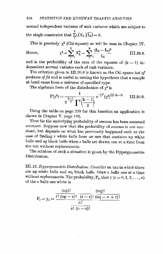
104 STATISTICS AND HIGHWAY TRAFFIC ANALYSIS
normal independentvariates of unit variance which are subject to k
the single constraint that I(Xi rf t-1) 0. This is precisely 2 (Chi-square) as will be seen in Chapter IV.
k k (fol - fti)2
Hence, 2= V, = ;' i fa II1.20.8. z
and is the probability of the sum of the squares of (k - 1) in
dependent normal vaxiates each of unit variance.
The criteriongiven in III.20.8 is known as the Chi-square test of
goodness offit and is useful in testing the hypothesisthat a sample
at hand came from a universe of specified type.
The algebraic form of the distribution of ) is
I _1_%. (X2) 2 P(z') = '-" (k e 111.20.9.
2 2 \ 2
Using the table on page 220 for this function an application is
shown in Chapter V, page 163.
Thus far the underlying probabilityof success has been assumed constant. Suppose now that the probability of success is not con
stant, but depends on what has previously happened such as the
case of finding r white balls from an urn that contains np white
balls and nq black balls when s balls are drawn one at a time from
the urn without replacements.
The solution of such a situation is given by the Hypergeometric
Distribution.
III. 21. Hypergeometric Distribution: Consider an urn in which there
Are np white balls and nq black balls. Draw s balls one at a time
without replacements. The probability, P,, that r (r 0, 1, 2, . .. ' S)
of the s balls are white is
(np)! (nq)!
r! (np - r)! (s - r)! (nq - s + r)! P7 Y" = , , I - - /
n !
s! (n - s)!

STANDARD DISTRIBUTIONS 105
(np)! (nq)! s! (n - s)! H1.21.1.
(np - r)! (nq - s + r)! n! r! (s - r)!
To illustrate: Consider the case of 100 vehicles approaching an
intersection of which np = 30 are trucks and nq = 70 are not
trucks. Consider any s = 5 of these vehicles one at a time. The
probability, Pr.= P. that 3 of the 5 vehicles are trucks is
30! 70! 5! 95!
P3 27! 68! 100! 3! 2! = 0.117
which means that 117 times out of 1000 sets of 5 vehiclesthe probability is that 3 vehicles out of 5 will be trucks.
Now, let
dy)X = r + I and y (yr + y,.+,)/2 and - = Yr+1 - Yr
(dx (x, y)
Then,
dy Yr s +nps-nq-1-r(n +2) III.21.2.
dx(,, Y) (r + 1) (r + I + nq - s)
From y = (yr + yr+,)/2, it is found that
-1 nps +nq + I-s-r(nq + 2-np-2s) +2r2
2 Yr (r + 1) (r + I + nq - s) III.21.3.
Replacing r by x - -21, III.21.3. becomes
I Idy\ 2s +2nps-2nq-2-(2x-1)(n +2) - W =
dx nps +nq+l-s +(x- ')(nq +2-np-2s) +2 Y (X - -2'-)'
III.21.4.
The equation given in III.21.4. is the equation of the system of
curves which are continuous approximations to the law of prob
ability given in 111.21.1.
The curves are usually known as the Pearson system of fre
quency curves which are the particular solutions of the differential
equation III.21.4.
The equation III.21.4., may be written in the form
/dy y (x +a) III.21.5.
b,) + b,. x + b2X2

106 STATISTICS AND HIGHWAY TRAFFIC ANALYSIS
which has 12 particular solutions or 12 specific types of curves
dependent upon the values of the constants." The moments about the arithmetic mean of the distribution
III. 2 L L, are
spq (n - s)
n - I
spq (q - p) (n - s) (n - 2 s)
(n - 1) (n - 2) III.21.6.
spq (n- s) _ [n(n+l)-6s(n-s)+3pqfn2(s-2)-nS2+ 6s(n-s)j]V-4 (n-1)(n-2)(n-3)
nllr+i I (I + E)r - Er1 [112 nP + s (q -p) [II + { spq (n - s) III.21.7.
where E is an operator and means that
Etr tir+j (r 0, 1, 2)
The maximum term of III.21.1. is approximately5
n III.21.8.
V2 pqs (n - s)
If in 111.21.6. and III. 21.7., n --* oo , the respective moments be
comethe momentsof thebinomialdistributionwhichshows thatthe
binomial or Bernoulli distributionis the limitingcase (or the case of
a large or infinite universe) of the hyper-geometric distribution(or
the case of a finite universe).
111. 22. Correlation6: The theory of correlation is devoted to the en
deavor of finding laws of relationship (dependence) between two
or more variables. Suppose a group of individuals is measured in
regardto a certain attribute. It is found that the individuals differ
in their measurements.It is desired to explain these differences in
terms of factors on which this attribute is dependent and to obtain
laws connecting the attribute with one or more such factors. The
better thelaw of connection explainsthe variabilityin the attribute
in question, the higher is the correlation.
To illustrate: One may wish to know whether the height of an in
dividual can be explained or measured by the weight of an in

107 STANDARD DISTRIBUTIONS
dividual. In other words, are tall people heavy and short people not heavy. It is well known that weight alone does not measure height or explain the difference in the height of individuals. In this instance there are more factors than the one factor weight.
There are three main types of correlation: simple correlation, multiple correlation, and partial correlation. These will now be developed and discussed in the order named.
The Correlation Coefficient r-Linear Regression or Linear Trend. The regression or trend line is necessarily the best fitting line in the sense of least squares. The line may be curved or straight. To start with, let it be assumed that the regression (trend) line is a straight line. The equationof this line is
y = mx + b III.22.1.
The values of m, and b must be determined and they are, respectively, the slope and y-intercept of the line. The x and y values are observedin pairs and they are the coordinatesof any point on the line. The formula 111.22.1. describes an infinite number of lines, eachwith its m, as well as its b. No two differentlines have the same m, as well as the same b. If the lines are parallel, they have the same m, but differentb's. If the lines pass through the same point on the y-axis, they have the same b but different Ws. We assume that any one of the possible lines has the same weight as any other one in arriving at a particular line, namely, the line that fits the data best in the theory of Least Squares. The Principle of Least Squares, used to determine the line of best fit, states that the line of best fit for a series of values is a line such that the sum of the squares of the vertical distances from it will be a minimum. There can obviously be only one line having this qualification. Another such line exists for the horizontal distances. However, the one for vertical distances is sufficient for most practical purposes.
In Figure IIIA., suppose that the line RR' is the straight line of best fit for the plottedpoints (scatter diagram) shown, and that its equation is
y = mx + b III.22.1.

108 STATISTICS AND HIGHWAY TRAFFIC ANALYSIS
The y-distance, namely, y', of any point (xi, yj) from this line
is equal to
yj - (mxi + b) III.22.2.
y
(Xi'yP
R'
M. + b
b go X
FIGURE III. 4
IIJUSTRATION OF PRMCIPLE OF LEAST SQUARES
The sum of these distances squared must be a minimum. Sym
bolically, n
d2 (mxj + b _ y,)2 III.22.3.
is to be a minimum. This necessitatesthat
ad n - = + 2 (mxj + b - yj) 0 III.22.4. Ob
and
ad n - = + 2 xi (mxi + b - yj) 0 III.22.5. am
From III.22.4.: n n
Zi yj nb + m Eixl III.22.6.

109 STANDARD DISTRIBUTIONS
where n equals the number of cases or number of points. From
III.22.5.: n n n
xi yj b xi + m x? III.22.7.
Equations III.22.6 and III.22.7 are so-called "normal" equa
tions for finding the least-square straight line. The two equations
can be solved simultaneouslyto find the unknownsm and b. These two equations are all that are needed to determine the equation
of the line of best fit. This line gives the relationshipbetween the
two variables x and y.
The procedure can be illustrated by an example. The required
calculationscan be done quite rapidlywith tables and a calculating
machine.
Example: Given the associated pairs of values for x and y:
x: 3, 5, 8, 12, 17, 23, 30
y: 1, 2, 6, 23, 40, 50, 60
Using these values in equations III.22.6 and III.22.7, it is found
that 182 7b + 98m
3967 = 98 b + 1960 m
Solving these equations for b and m, we find that m = 2.41 and
b 7.78 whence y = 2.41 x - 7.78 III.22.8.
is the equation of the best fitting straight line. From III.22.6
mx + b - y = 0 III.22.9.
The equation III.22.9. expresses the fact that the linear function
(straight line) passes through the point whose coordinates are
(x, Y)
Now measure all the x's and y's from their respective means as
origin and replace every x by its deviation x' from _x, and y by its
deviation y' from _y. Then III.22.9. becomes, since b now is zero,
y Mx, III.22.10.
and III.22.7 becomes
m n 1 X/2 n
It xi' A = 0

110 STATISTICS AND HIGHWAY TRAFFIC ANALYSIS
from which n El xi yi np p
III.22.11.G2 G2 El XI'2
It follows that Py _X/G2X
whence P
YX y - (X___O 111.22.12.
It is important to note that is the computed value of y for a given x from the equation of the least-square line. For the line to be a regression (trend) line, it is necessary that _YX is thearithmetic mean (or close to being so) of the values of y associated with a given value of x.
Similarly
XY- x -p
ya2(y- y III.22.13.
The coefficient p/a 2 gives the deviation in y from the mean y corresponding to unit deviation in x from the mean x, for when * - X= 1, Y" - y p/a.,,2. Likewise, p/ay gives the deviation in * from the mean x corresponding to unit deviation in y from the mean y.
But, in general, p/CF2y_* p/a,2,. This demands the necessity of altering the unit of measure so that unit change in x and y are of the same magnitude. Then
Y.-Y= P x X)( III.22.14. Ily ax ay ax
and _Xy p y:j III.22.15. ax
Next, write
p axay
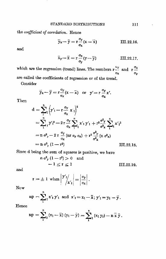
STANDARD DISTRIBUTIONS
the coefficient of correlation. Hence - - cry YX-Y==r (X--X) III.22.16.
ax and
ax xy- x =:= r - (y- y) III.22.17.
ay ax
which are the regression (trend) lines. The numbers r Y and r ax ay
are called the coefficients of regression or of the trend.
Consider
YX Y Y
r S- (x -X) or ay
y'= r - x'. ax ax
Then
d I-r- ay X )2
I (Y G. n
Y'? 2 r n
'Y E ax
XI, y',
a2 n
+ r2 Y 'Y 2
ax X/12
n a2y - 2 r ay (nr ay ax) + r2 a2y (n o2x) ax a2x
n a2y (I - r2) III.22.18.
Since d being the sum of squares is positive, we have
n a2y (I - r2) > 0 and
- 1 :! r -< I III.22.19.
and
r I when Y'XXII ay
Now n
np x'i y'j and XI, xi - -X; y', yj - Y
Hence n n
TIP (xi - X) (Yi - Y-) (XI YO - I"X Y.

112 STATISTICS AND HIGHWAY TRAFFIC ANALYSIS
Hence
El xi yl p _xy.n
But
r p Gx CY
Hence n n jj:Kj Yj El Xi yi
n n r
ax ay n El X? El y?
- (jE)2 /1n - I _
-(y)2
n n n El (XI-X) (yl-_y) El Xi" yi" El Xi' yi
III.22.20, n ax ay n n ax ay
From this relation, it is fairly clear that r may be considered as the cosine of the angle between two vectors in Euclidean n space. Again, from this fact, it follows that - I :< r :: 1. Also, r is the arithmetic mean of the products of the deviations of the corresponding values from the respective arithmetic means when measured in standard deviation units; also, r is sometimes called the product-moment coefficient.
The formulas useful in findingthe value of the coefficient of correlation are as follows:
(1) If the variables are in original units with respect to their natural origin, then
n El xi Y1
_xy Ill. 22. 21. n
r ax ay

113 STANDARD DISTRIBUTIONS
(2) If the variables are referred to a class mid-point as an origin
and in terms of the class interval as a unit, then
n
ll xi yl __xy n III.22.22.
r = crX ay
These formulas are readily obtained algebraically from III. 22. 20.
To interpret r, it is necessary to use r2 which is called the deter
mining coefficient.
If r, say, equals 0.70, we find that r2 = 0.49 which means that
49 per cent of the variability in the y-values is determined or
explained by the potential determiningor measuring factor x and
the linear theory connecting y with x. In other words, the theory
used or tested is but 49 per cent efficient as an estimator or
forecasting or predicting theory.
III. 23. Basic theory of correlation. To explain the Basic Theory of
Correlation let us suppose that we have given n pairs of values for
the variables x and y. The problem is to determine the nature
and degree of the dependence between the x values and their
corresponding y values.
To determine the amount of interdependence that exists be
tween the pairs of variables it is convenient to represent them by
points in a two dimensional Euclidean manifold (scatter diagram).
To facilitate a description of the dependence we partition the data
into classes. This is accomplished by selecting class intervals of size
dx. We recall that the set of y values associated with a given value
of x on an interval of size dx is called an x axray of y's. If it is de
sired to describe the behavior of the expected values of the y val
ues associated with the x values, it is necessary to find the equation
of the curve y = f (x) that passes through these points. This curve
is known as the estimate of the true regression curve. The limiting
curve that is approached as dx tends toward zero is the true
regression curve (trend) of y on x and is actually the locus of the
arithmetic mean of arrays of y values of the theoretical distribu
tion as dx tends toward zero. The description of the theoretical

114 STATISTICS AND HIGHWAY TRAFFIC ANALYSIS
law of behavior appertaining to the arrangement of y is the solution of the problem of statistical dependence (regression or trendanalysis) of y on x.To illustrate: Consider the related value of minimum spacing,center to center in feet, with speed in miles per hour.
Table III.4. is a correlation table which shows numerically as well as graphicallythe two-way distribution connecting minimum spacing, center to center in feet with speed in miles per hour as found by actual observation. The first question to be answered is: How dependent upon the speed of a vehicle is the minimum spacing? The answer to this question is found in interpreting the value of the determining coefficient which is the square of the correlation coefficient.
Substitutingin III.22.22 the required values from Table III..,4 it is found that
1 (xy) n
r ax ay
becomes 47440 3321 J-9849
13-36 F13365 1336 r=
58771 I- 332121/H113049 t-984921336 336
y V 1336
35.509 - 2.486) (- 7.372)
Y44.090-6.18OV84.618-54.346
35.509 - 18.327 17.182
(6.149) (5.502) 33.832
0.5079 0.51 III.23.1.
This result means that (0.5079)2= 0.2580 = .26 = 26 per cent of the variabilityin minimum spacingis explainedby or dependent upon the speed of the vehicle and the assumed linear connection between spacing and speed. In other words, it appears that speed is an unimportantor minorfactorfor determiningminimumspacing.

Table IIIA
Speed in miles per hour
01 oil 1, I I 1, H N N N 04 04 M MM M M
01 all "I 'IC .10 C', N,4WI .10 01 I'D .10 0110 C11 el el] aq aqM M M'IV -IV
131-134 127-130 123-126 119-122 - - - - - - - - - - - - -I- - - - - - -115-118 1 I I 111-114 1 1 1 11
710-7 - 1-10 - - - - - - - - - -1-2 - -1 -1 - -2 - - - - - - - 1 103-106 3 1 11 2 1 1
99-102 11- 2 1 9 8 1 2
23 1 212 12 01-94 11 4 1 87-90 I 45 4161 1.I 83-86 1 133 2152 23 79-82 1 1 1 11 1 2212 3 2 275-78 1 21 2 335 411 1
bo 71-74 I 3 55 i 73412
-6-7-70 - - - - - - -I- - -1-2 -4 -2 -2 -1 3 -4 -3 -5 -412 - - - -C'c 673--66 2- - -1-3 -1 -2 -3 -1 -1 H -3 T2 -2 -6 -3 -2 -1---- -
5-9--62 - - -1 - - -1- -1 -1 -2 -3 - -6 FO -9 -6 -2 -4 -1--2 -1 I 1 -3 -2 -11-3 -4 -2 -9 9 H 54 41 -1
-2 1 -2 -1 -1 -2 -3 -3 -2 -9 -8 -6 -9 -6 -2 -3 -1 0--50 -3 -4 -2 - -2 -2 -1 -3 -3 -4 -4 -3 1-7 -6 -9 -4 -6 -7 1-13--46 -1 - -6 -2 -6 -4 -7 -1 -3 -1 - - 1-4 -8 1-1 1-1 -3 -4 - 1 - -1 39-42 -3 -2 -7 T3 -9 9 -3 -6 -2 -6 -6 -7 -2 1-9 0 -8 -6 -2 -3 -3 -1 -1
7M5--38 -4 1-2 -9 1-4 -2 -5 -5 -3 -2 -3 -7 Hl 1-4 -5 3 -7 1-0 -2 1-2 - 1 -31---34 -6 -6 -9 -6 -6 1-1 -3 -5 -5 1-1 -2 -6 -6 1-0 -9 -5 -5 -3 -3 -1 - -
27-30 2 F6 1-7 -8 -7 -8 -6 -1 -8 -6 -8 -6110 5 2 51 I 1 -3--26 5 14 59 1-7 -4 -2 -2 -5 -6 -3 -1 -4 -5 -5 -1 -2 -
I-9--2-2 3 i73 -3 -3 -4 _3 -2 -1 -1 -1 -2 6 2 2
1
----------------------
-------------- -----------
---------------------------
---------------------- ---
--
--
--
-------------
fy
2 3 2
2 1 3 6 8 1 5
1 7
23 23 20 24 32 35 54 51 61 61 82 85
129 126 118 153 123
67 10
1336
y
16 15 14 13 12 11 10
9 8 7 6 5
3 2 1 0
- I - 2 -3 - 4 - 5 -6 - 7 - 8 - 9
- 10 - 11 - 12 - 13 - 14 - 15
fy (Y)
32 45 28
24 11 30 45 64 7 7 so 85 40 69 46 20
- 32 - 70
- 162 - 204 - 305 - 366 - 574 - 680
- 1161 - 1260 - 1298 - 1836 - 1599
- 798 - 150
9849
fy (Y,)
512 675 392
288 121 300 405 512 539 180 425 160 207
92 20
32 140 486 816
1525 2196 4018 6440
10449 12600 14278 22032 20787 11172
2250
113049
5 8 5
14 -1
4 4 9 1
1 2 3 7
3 8
24 24 40
102 76 75
129 64
0 8
- 43 - 345 - 401 - 410
- 1001 -1047 - 603 - 122
3321
YNX
80 120 70
168 - 11
40 36 72 7
72 185
1 2 24 48 24
- 102 - 152 - 225 - 516 - 320
- 56 344
3105 4010 4510
12012 13611
8442 1830
47440
M M ID C 10 H XC M N H 10
H 0 0 CO 0 H H C11 M O 10 t 00 C 0 cl M
'2 2 -HI
.0 00
0'O
00
CO 0c H 'DM
10HN10NH Mo=IDM CqMcl M
MCM C4 d
C C
0 10 H
0 C- -,6v N
'O- -:5 6 cl M
-C; - -06 -6 -L-: -4 - - - - - -4 0 H IM 10 ,
- -M 0
- - - -C.M0 10 10
-0 C ',M

115 STANDARD DISTRIBUTIONS
This means that either there are several other factors which to
gether would explain 74 percent of the variability or that there
exists a possible single other factor or that the relationship is not
linear. Of these, it appears that the former is the most likely.
A second question that needs to be answered is: What is the
equation of the linear law of relationshipwhich is useful to predict
the expected minimum spacing when the speed is known.
To answer this, it is necessary to use the regression equation
III.22.16, namely:
YX_ y r!-y (x- X-) ax
Substituting the values indicated by the use of Table IIIA. and
III.23.1, it is found that
22.008 yx - 47.0 0.508 - (x - 22.0) III.23.2.
12.300
whence
y, 0.909 x + 27.0
The graph of this equationis shown in Figure III. 3. To illustrate the use of 11I.23.2, suppose it is desired to know the minimum
spacing in feet if the speed is, say, 30 miles per hour. To answer
this question, substitute 30.0 for x in equation III.23.2, whence
the minimum spacing Y,, is found to be 54.3 feet. This means that
the expected minimum spacing center to center in feet or on the
average the minimum spacing center to center in feet is 54.3 feet
when the speed is 30.0 miles per hour.
A very important question now to be answeredis: How typical
or reliable is the expected minimum spacing of 54.3 feet. This
question will be answered in article 111.25.
III. 24. Coefficient of Regre88ion: Consider n
11 n., (yy.,X, - mxj - b)2
For f to be minimum
af 0 and Of = 0. III.24.1. am Lbb

116 STATISTICS AND HIGHWAY TRAFFIC ANALYSIS
From equations III.24.1., n ny -
nx, yn'jXi Y-inx Xi yn.,/n M
n n n't X2i El nx, x2j/n
n
Y-1 (xi yj)/n r ax: av aya-
ax ax
III. 25. Standard Deviation of Arrays:
Consider S2 n 2
n E r ay x 1 (Y ax i) n ay n Y2
zi y?- 2rE1(ylx1) + r, 51, x2 1 ax I
= n ay 2 nr2 a2 y + nr2 Cy2y n cr2 k2)
y
Hence: s2
y = ay r2) III.25. 1.
SY may be regarded as a sort of average value of the standard deviations of the arrays of y's and is sometimes called the root-mean-square error of estimate of y, or more briefly, the standard error of estimate of y. The factor (I _ r2) is called the coefficient of alienation or the measure of the failure to improve the estimate of y from the knowledge of correlation.
if SY is regarded as a function of x, say S (x), the curve
y = S W ay is called the scedastic curve. Its ordinates measure the scatter in the arrays of y's in comparison to the scatter of all the y's. If S (x) is a constant, the regression system of y on x is called a homoseedastic system. If S (x) is not a constant, the system is said to be heteroscedastic.For a homoscedasticsystemwith linear regression, Sy ay (I - r2)1 is the standard deviation of each erray of y's.
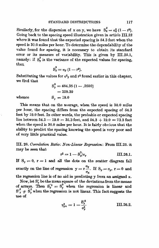
STANDARD DISTRIBUTIONS 117
Similarly, for the dispersion of x on y, we have S;2 = aX2 (I - r2).
Going back to the spacing speed illustrationgiven in article 111I.22
where it was found that the expected spacing is 54.3 feet when the
speed is 30.0 miles per hour. To determinethe dependabilityof the
value found for spacing, it is necessary to obtain its standard
error or its measure of variability. This is given by III.25.1, namely: ff S2Y is the variance of the expected values for spacing,
then 2
SY = (Ty (I
Substitutingthe values for a2y and r2 found earlier in this chapter,
we find that S
2Y = 484.35 (1 -. 2580)
= 359.39
whence Sy = 19.0
This means that on the average, when the speed is 30.0 miles
per hour, the spacing differs from the expected spacing of 54.3
feet by 19.0 feet. ID other words, the probable or expected spacing
lies between 54.3 - 19.0 = 35.3 feet, and 54.3 + 19.0 = 73.3 feet
when the speed is 30.0 miles per hour. It is fairly obvious that the ability to predict the spacing knowing the speed is very poor and
of very little practical value.
III. 26. Correlation Ratio: Non-Linear Regremion: From III.25. it
may be seen that 2
r2 = I - Sy-lay III.26.1.
if SY ;== 0, r = 1 and all the dots on the scatter diagram fall
exactly on the line of regression y r Sy-. If Sy ;--- ay, r 0 and ax
the regression line is of no aid in predicting y from an assigned x.
Now, let S'Ybethemean square of the deviationsfrom the means of arrays. Then S,, 82 when the regression is linear and S/2 2 y y
Y =P S. when the regression is not linear. This fact suggests the
use of
2 SY,2 III.26.2.YX 62
Y

118 STATISTICS AND HIGHWAY TRAFFIC ANALYSIS
where 71y. is the correlation ratio of y on x and S12 is the mean
square of the deviations from the means of arrays whether these
means are near to or far from the proposed line of regression. For lineax regression of y on x, we have n2yx k2. Similarly for x on y,
we have '2
2 I- X My = ex III.26.3.
To illustrate the finding of the value of correlation ratio which
actually is the true measure of correlation, the procedure is to find
7)2YX from equation III.26.2. where 12
2 -SY. 7)YX aY2
As was explained, (Sy')2 is the mean square of the deviationsfrom
the means of arrays, namely
f, S2 + f2 82 . ..... + f, S2 + ... + f2 2 (SY')2 1 2 n I k sk 11I.26.4.
where f, is the frequency of the ith verticalarray - the array when
x has the value xi and s2 is the variance of the ith array. From
III.26. 1., it is clear that fj 0, is actually the sum of the squaresof
the deviations of the values for the ith array of y's fromthe arith
metic mean of the i th array of y's.
Making use of Table I111.4., it is found that, beginningwith the first array of y's, namely, the array of y's when x = 0.95,thenthe
second array when x = 2.95 and so on...,
f, S21 f2 S222 (40.5 - 23.1)2 + 1 (44.5 - 27.0)2 +
1 (36.5 - 23.1)2 + 3 (40.5 - 27.0)2 +
4 (28.5 - 23.1)2 + 4 (36.5 - 27.0)2 +
19 (24.5 - 23.1)2 + 6 (32.5 - 27.0)2 +
23 (20.5 - 23.1)2 + 22 (28.5 - 27.0)2 +
6 (16.5 - 23.1)2 24 (24.5 - 27.0)2 +
1355.9 13 (20.5 - 27.0)2 + 2 (16.5 - 27.0)2
= 2364.7
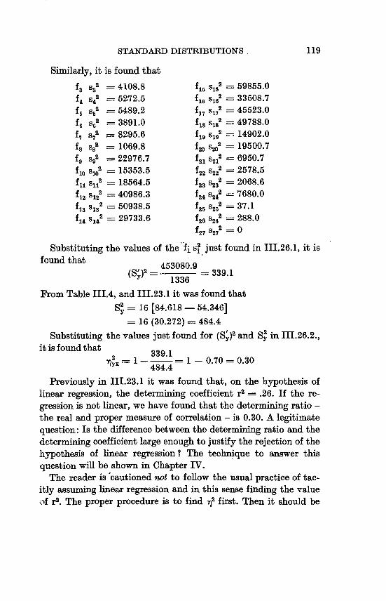
119 STANDARD DISTRIBUTIONS,
Similarly, it is found that
f3 S32 4108.8 fl, s152 = 59855.0 f4 s 42 = 5272.5 fl, S162= 33508.7
f5 S62 = 5489.2 fl, S1,2 = 45523.0 f, 8 62 = 3891.0 f18 S182 = 49788.0
f, S72 8295.6 f19 8192= 14902.0 f8 S 82 1069.8 f2oS 2D2 19500.7
f9 sq 22976.7 f2l 8212 6950.7 floS 2 15353.5 f22 S22 2578.510 2
fil Sil2 18564.5 f23 S232 2068.6
f12 S122 40986.3 f24 S242= 7680.0 f13 S132 50938.5 f25 S252= 37.1
2 2f14 S14 29733.6 f26 S26= 288.0
f27 S272= 0
Substituting the values of the s? just found in III.26.1, it is
found that (SI)2 = -453080.9 = 339.1
Y 1336
From Table IIIA, and III.23.1 it was found that S2 = Y 16 [84.618 - 54.346]
= 16 (30.272) = 484.4
Substituting the values just found for (SY')2 and S2Y in III.26.2.,
it is found that 2 = 1 - 339.1 = I - 0.70 = 0.30 YX 484.4
Previously in III.23.1 it was found that, on the hypothesis of
linear regression, the determining coefficient r2 = .26. If the re
gression is not linear, we have found that the determining ratio
the real and proper measure of correlation - is 0.30. A legitimate
question: Is the difference between the determining ratio and the
determining coefficient large enough to justify the rejection of the
hypothesis of linear regression? The technique to answer this
question will be shown in Chapter IV.
The reader is ,cautioned not to follow the usual practice of tac
itly assuming linear regression and in this sense finding the value
of r2. The proper procedure is to find 2 first. Then it should be

120 STATISTICS AND HIGHWAY TRAFFIC ANALYSIS
determined whether 2 is large enough to justify the obtaining of the actual regression (trend) function as well as whether 7)2 is large
enoughto indicate that a significant correlation exists. The former is discussed and shown in 111.29. and the latter in Chapter IV.
In the case just illustrated it is true that 12 = 0.30 indicates real correlation, but it is much too small for predicting or estimation purposes. It is also true that there are sufficient grounds, as will be seen in III.29. to reject the hypothesis of linear regression.
A mean square of the deviations in each array is a minimum when the deviations are taken from the mean of the array. Hence, the (SI)2 in III.26.2. must be equal to or less than S2 in III. 26. I.
y yfor the same data, since the deviations in III.26.1. are measured from the proposed line of regression. Hence, we have shown that
'-_ -2 > r2 It follows from III.26.2. that 71Y. :: 1.
If regression of y on x is linear, 7)'YX - r2 found from the sample differs from zero by an amount not greater than fluctuations due to random sampling. A comparison of 7]2YX- r2 with its sampling error is a useful criterionfor testing linearityof regression. A better and more powerful method, however, to test linearity of regression is by the use of the Analy8i8 Of Variance.
III. 27. Multiple Correlation: Suppose we have given N sets of correspondingvalues of n variables XP X21 ... I X-' Now separate the values of xi into classes by selecting class intervals dX21 dX31 ... I
dxn of the remaining variables. The locus of means of such arrays of xi's in the theoretical dis
tribution, as dx2l ... dxn approach zero is called the regression surface (trend) of xi on the remaining variables. We now assume, for convenience, that any variable, xj, is measured from its arithmetic mean as origin. Let cFj be its standard deviation and let rpq be the correlation coefficient of the n given pairs of values of xp and Xq. We now seek to find b12, bi3, ... ' bin of the linear regressionsurface
xi = b12 X2 + b13 X3 + + bin Xn + C I[II.27.1. of xi on the remaining variables so that xi computed from III.27. I. will give the best estimates in the sense of Least Squares

STANDARD DISTRIBUTIONS 121
of the values of x, that correspondto anyassigned values of X21 ... I
xn. It follows that
U Z (xI - b12 X2 - b13 X3 bin xn - 0)2 III.27.2. shall be a minimum. This gives us for the linear regression surface
n Riq Xq XI CI Yjq III.27.3.
2 R,, aq
where rl,, r.2, ... , r,,
r2j, r221 r2n
R
full rn2l . . .I rn,
and Rpq is the cofactor of the pth row and qth column of R.
If the dispersion al-2. - - - - of the observed values of XI from
computed values is defined as
a21.23. n -1 Z (observed x, - computed XJ)2 III.27.4. n
then, it can be proved that
a21-23 ... n P. III.27.5. R_111
We are next interested in the dispersionof the estimated values
given by III.27.3. Since the mean value of the estimates is zero,
when the origin is at the mean of each system of variates, it can
be shown that
C12 2 i-R Eal III.27.6.
The square of the multiple correlation coefficient rj-2, ... n of
order (n - 1) of XI with the other n - 1 variable is given by
r21-23 ... n 1 - I R III.27.7. Rjj
The analysis of datafurnished by J. S. Ellerby, SafetyDirector,
Fort Belvoir, Virginia will serve as an example of multiple cor
relation. These data consist of the following information on 440
drivers: XI = Road Test
X2 Years of Experience

122 STATISTICS AND HIGHWAY TRAFFIC ANTALYSIS
X3 = Reaction Time X4 Distance Judgment X5 =Driver Information (Written test)
Let us assume that the road test is a measure of driver ability and let it be our problem to determine whether each of the other tests individually or collectively measure driving ability.
The first step is to determine the simple correlation between each of the tests. The procedure for this is that followed in the example of finding the correlation between speed and minimum spacing.
These correlations are shown in Table IIIA Before using these results to obtain a multiple correlation let us consider the significance of these simple correlations. It is noted immediately that none of them is large enough to be significant and therefore our conclusion is that none of the tests is of value as a measure of driving ability.
Table 111.5 SiimPLECoRRELATioN oF DRIVERTESTS
(1) (2) (3) (4) (5) Road Test Years Reaction Distance Driver
Experience. Time Judgment Intormation
Road Test r,=1.0000r,,=.0476 r,,=.0257 r,,=.05514r,5=0.2608
(2) Yr8.
Experience r2,=.0476 r22=1.0000 r2,=.006157 r2,=.00101 r2,=-0.4603
(3) Reaction
Tim,e r,,=.0257 rl2=.006157 r,,=1.0000 r,,,=-.0404 r35=-.1027
(4) Distance, Judgment =.055141r_=.00191 r,,=-.0404 r,,=1.0000 r,,=.1568
(5) Driver
Intormationr, =u.2608rr,2=-0.4603 r,,=-.1027 r,=.1568 r,5=1.0000
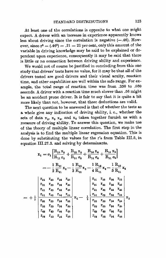
123 STANDARD DISTRIBUTIONS
At least one of the correlations is opposite to what one might expect. A driver with an increase in experience apparently knows less about driving since the correlation is negative (-.46). However, since r2 (.462) .21 21 per cent, only this amount of the variable in drivingknowledge may be said to be explained or dependent upon experience, consequently it may be said that there is little or no connection between driving ability and experience.
We would not of course be justified in concluding from this one study that drivers' tests have no value, for it may be that an of the drivers tested are good drivers and their visual acuity, reaction time, and other capabilities are well within the safe range. For example, the total range of reaction time was from .350 to .560 seconds. A driver with a reactiontime much slower than .56 might be an accident prone driver. It is fair to say that it is quite a bit more likely than not, however, that these deductions are valid.
The next question to be answered is that of whether the tests as a whole give any indication of driving ability, i. e., whether the sets of dataX21 X3 X4, and x5 taken together furnish us with a measure of driving ability. To answer this question, we make use of the theory of multiple linear correlation. The first step in the analysis is to find the multiple linear regression equation. This is done by substituting the values for the r's from Table III.5, in equation III.27.3. and solving by determinants.
x [R12 X2 , R13 X3 _,_ R14 X4+ RI, x5 _r KI, (73 RII (74
1K11 (72 RI, (Y51
1 R12 1 R13 1 P114 1 Ris X 2 X3_ j_X4--k-X52 RI, 3 RI, 4 11 5 11
r2, r2, r24 r25 r2, r22 r24 r25
r., r., r.4 r35 r3l r32 r.4 r.5
r4, r., r4, r4, r., r.2 r44 r45
+ I r., r.3 r54 r., 1 r5, r.2 r., r55
2 r.2 r23 r24 r25 2- -i r22 r23 r2, r2, -3
r.2 r., r.4 r35 r., r., r.4 r35
r.2 r4. r" r4, r4. r4. r44 r45
r.2 r., r.4 r., r., r., r.4 r5,

124 STATISTICS AND HIGHWAY TRAFFIC ANALYSIS
r2]L r22 r2, r2r, r2l r22 r23 r.4
r3i r32 r.3 r.5 r., r.2 r., r.4
r4, r42 r4. r45 rAj r42 r4. rA4
+ 1 r.1 r,52 r5, r5, X4 - I r., r.2 r53 r54 -5
4 r22 r23 r24 r25 5 r22 r23 r24 r2,
r.2 r., r.4 f35 r.2 r., r.4 r.,
r42 r4. r44 r45 r.2 r4. r4, r45
r.2 r., r,4 r,5 r52 r.3 r.4 r5,
_ f.0092 x2 -. 0460 x. -. 0030 x. -9.3281 I +_ - +_ i
.7532 11.4434 .7532.0452 .7532 10.2713
-. 2722 X5
.7532 2.73671
= -. 0016 X2 + .0253 X3 + .0036 X4 + 1.2318 x..
The next question that is to be answered is how reliable are the
expectedvalues of the xj's as determined from the regression equa
tion when sets of values for X21 X3 X4, and x,, are known. The square of the multiple correlation coefficient when properly inter
preted is the answer to this question.
This is equation II1.27.7
r2 R 1.23 . . . air,,)n
We first find R by substituting the values from Table III.5 for
its determinant and solving.
r1l r.2 rJL3 r14 r,5
r2l r22 r2. r24 r25
R r., r.2 r., r.4 r35 .6774 r4l r42 r43 r44 r4r,
r., r52 r., rr,4 r.,
Therefore, since R,, .7532 as determined above,
I P. .6774 31.2345 - = 1 -. 8994 = .1006
.7532
Since this value, .1006 means that only 10.06 per cent of the
variability in road tests is explained by the composite knowledge

125 STANDARD DISTRIBUTIONS
of the factors, years of experience, reaction time, distance judgment, and driver information, it may be concluded that the composite result of these tests is practically worthless as a measure of driving ability as shown by the road test.
Another question to be answered is what is the standard error in the expected values of x. This standard error is a measure of the total variability that is not explained, or in other words, is not dependent upon the sets of values of X21 X31 X41 and x,.
The standard error in the expected value of x, obtained from the regression equation III.27.5 is equal to
a12. ( R 2345 ali
al.2345 (TI [_R = 9.3287 6774VRI, Y.7532 0.8847 = 88.47 percent
Since
(R R 2 R 2 a, + a RI, 1
RI,) RI, we may say that the proportionalpart of the total variability (a')I
that is not explained in terms of X21 X3) X4, and x, is R = .8994 B11
89.94 per cent and that the explained variability
RI - - = 1 -. 8994 .1006 = 10.06 per cent.
RI, As a check:
+ I- R) =.8994 +.1006 = 1. RILI RI,
III. 28. PartialCorrelation: Very often we wish the degree of correlation bet*een two variablesx, andX2 when the othervariablesx3,
X42 ... xn have assigned values. Thus, we define a partialcorrelation coefficientr22-.4 ... n Of x., and X2 for assigned X31 X41 x. as the

126 STATISTICS AND HIGHWAY TRAFFIC ANALYSIS
correlationcoefficient of xi and X2 in the part of the populationfor
which x3, X41 ... xn have assigned values. A change in the assigned
values may lead to the same or different values of r12-34 ... n,
Assume that the theoretical mean or expected values of xi and
X2 for an assigned X31 X41 . . ., xn are
xi b13 X3 + b14 X4 + + bin xn III.28.1.
X2 b23 X3 + b2d X4 + + b2n xn respectively.
Then, a partial correlation coefficient r'12'.4... 11 is the simple correlation coefficient of residuals
XI-34 ... n xi - b13 X3 - b14 X4 - bin xn III.28.2.
IX2-34 ... n X2 - b23 X3 - b24 X4 - b2n J
limited to the part of the population n34 ... n of the total n for
which x3, X41 . . ., xn are fixed.
Suppose further that the populationis such that any change in
the assignment of values to x., X41 - - -, Xn does not change the
standard deviation of X1-,4- .. n nor of X2.34 ... n nor the value of
r,2..4 n, Such a population suggests that we define
r.2-34 ... XI-34 ... n X2.34 ... n III.28.3.
nal-.4 ... n a2.34 ... n
where the summation extends to n pairs of residuals, as the partial
correlation coefficient of xi and X2 for all sets of assignments of
X3 - - -, Xn-
If the population is such that r'.2-34 ... n is not the same for each
different set of assignments of x., X41 ... xn, the right hand member
of III.28.3. may still be regarded as a sort of average value of cor
relation coefficients of xi and X2 in subdivisions of a population
obtained by assigning x., X41 - - -, xn or it may be regarded as the
correlation coefficient between the deviations of xi and X2 from
the corresponding predicted values given by their linear equations
on x3, X41 ... Xn- It can be shown that
r - - - R12 III.28.4.12-34 ... U
(RI, R22)'
To illustrate, we make use of the data for the Driver tests prev
iously given in Table III. 5 and set ourselves the problem of finding

127 STANDARD DISTRIBUTIONS
the correlation between road test and years of experience under the assumption that each is influenced to some extent by reaction time, distance judgment and driver information. If each is thus influenced, the obtainment of the simple correlation coefficient between the road test and driver experience, assuming the existence of such influence, gives us spurious correlation. Partial correlation between road test and years of experience is the theory of correlation that removes the influence of reaction time, distance judgment, and driver information. Substituting the probable values of the R's for III.28.4, we find that
- R12
r.2-34 (R11 R22)
Wherein R12 and R,1 have the values already determined and R22 has the value .8960 found by substituting values from Table 111.5. and solving the determinant.
r,1 r.3 r.4 r15
r3, r.3 r34 r35
R22 r4l r43 r44 r45 = -8960 r,,. r.3 r,,, r.,
hence
-R12 .0092 -. 0092 -. 0092 r.2-3. - - _=__ - - - _0.001
(R11 R22) R7532) (.8960) V.6749 .821.5
therefore, there is practicallyno partial correlation.
III.29. Regression (Trend) Lines: Let Y;== ao + a, X + a2X2 + + a,,XP 111.29.1.
be the equation of expected values of Y that are associated with the various values of X. It is desired to know the values of the a's such that the value of U given by
n U g--- Y-i (y, - ao - ajL xi - a2X2 apXP)2 III.29.2.
IL
is a minimum.
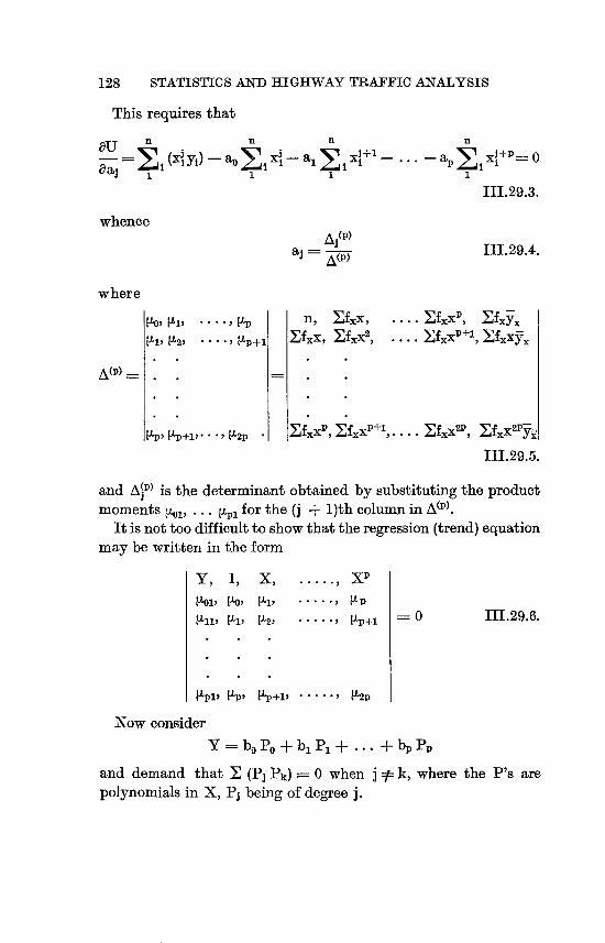
128 STATISTICS AND HIGHWAY TRAFFIC ANALYSIS
This requires that
OU n n n n xl+p O - E, (xi yi) - ao'y,, xi - a., xl,+' - apOaj
III.29.3.
whence
a, = AJ(P) 111.29.4.Am
where
(lo, 14. ..... P-P n, Efxx, Vxxp, Efxy-x (11, IL21 .... I 'P+l EfXXI EfXX21 .... EfXXP+ll vxxy"
A(P)
J&XP, EfXXP+I,.... Ef.XV, EfXX2P[1p, [4p+j, 12p YJ
III.29.5.
and A(P) is the determinantobtained by substitutingthe producti moments RI, t4pi for the (j + 1)th column in A(P).
It is not too difficult to show thatthe regression (trend) equation may be written in the form
Y, RI, 1111,
I, P-O, (11,
X . [Li. tL21
...... ...... ..... I
XP tLp
[4P+1 0 111.29.6.
14pl) P-P, h+11 ..... I IL2P
Now consider Y=b,,Po+bPl+ ... +bpPp
and demand that Z (Pj Pk);== 0 when j 4= k, where the P's are polynomials in X, Pj being of degree j.
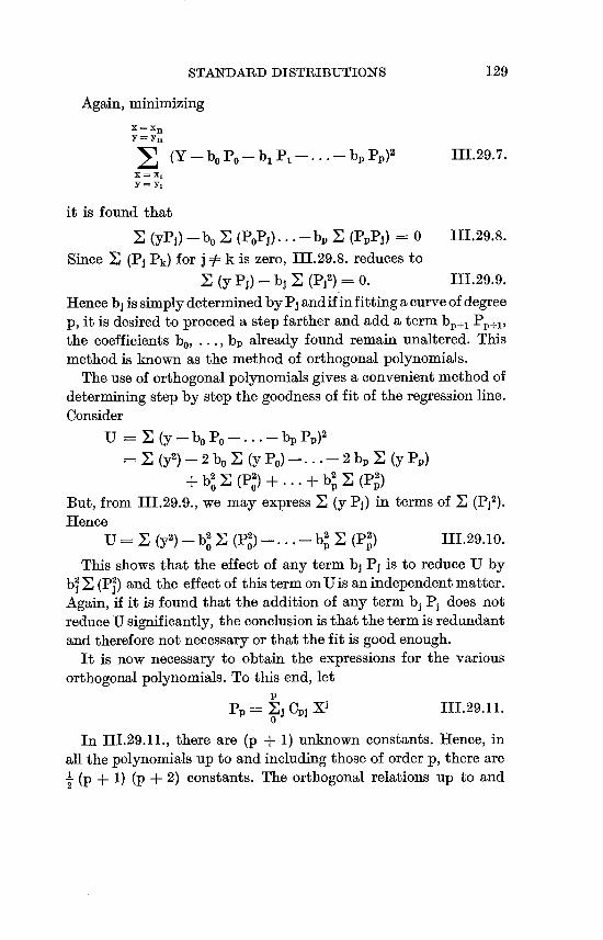
STANDARD DISTRIBUTIONS 129
Again, minimizing
X=X,Y=YU Y (Y-b0P0-bjP,-...-bpPr,)2 II1.29.7. X=XY=Y1
it is found that
Y, (yPj) - bo E (PoPj). . bp Y- (PpPj) 0 III.29.8. Since E (Pj Pk) for j =p k is zero, III.29.8. reduces to
(y Pj) - bj Y_ (PJ2) 0. I11.29.9.
Hence bj is simplydeterminedbyPj andifinfittinga curve ofdegree p, it is desired to proceed a step farther and add a term bP+1 PP+1) the coefficients bo, . . ., bp already found remain unaltered. This method is known as the method of orthogonal polynomials.
The use of orthogonalpolynomials gives a convenient method of determining step by step the goodness of fit of the regression line. Consider
U (y - bo Po - bp Pp)l (y2) - 2 bo Y- (y PO) -. . . - 2 bp E (y Pp)
+ b2' E (PO2) +... + b2 E (pP2)0 P
But, from III.29.9., we may express E (y Pj) in terms of E (PJ2).
Hence U'',(y2)-b'E(p2)_.. -b 2 E (pP2)
0 P II1.29.10. This shows that the effect of any term bj Pj is to reduce U by
b2 E (p2) and the effect of this termonU is an independentmatter. Again, if it is found that the addition of any term bj Pj does not reduce U significantly, the conclusion is that the term is redundant and therefore not necessary or that the fit is good enough.
It is now necessary to obtain the expressions for the various orthogonal polynomials. To this end, let
P PP EJ CPJ xi I11.29.11.
0 In III.29.11., there are (p + 1) unknown constants. Hence, in
all the polynomials up to and including those of order p, there are -' (p + 1) (p + 2) constants. The orthogonal relations up to and2

130 STATISTICS AND HIGHWAY TRAFFIC ANALYSIS
including order p provide I p (p + 1) conditions on the C's. It2
follows that ' (p + 1) (p + 2) - -1 p (p + 1) p + I constants 2 2
are assignable at will. For convenience, take one constant for each P and assignit so that the coefficientof XJ in Pj has the value unity. In other words, put
Cii . I III. 29.12.
Rewriting 111.29.11., we get Po = 1 P3 = Clo + X
PI C20 + C21 X+ X2 P3 ;7-- C30 + C31 X + C32 X2 + X3 III.29.13. ................. PP = CPO + CP1 x + CP2 X2 +... + XP
From the orthogonal relations PP Po ,E PP 0 PP P, = 0 III.29.14.
This system, 111.29.14., is equivalent to E PP = 0 x Pp = 0
xP PP = 0 III.29.15.
Substituting the values of the P's from 111.29.13., it is found that
CPO k + CP1 Ll ++ Cp, P-1 11P-l + 4P = 0 CPO Ill + CPl 42 ++ CPI P-3. ILP + 4P+1 = 0 111.29.16. .................
CPO tP-l + CPl tLP ++ CPI P- I V-2 P-2 + 42 P- I = 0
From these equations,A(P)
C'Pi pi III.29.17. A(P-1)
where A(P-1.'has the same meaning as before and A(P) is the minorPi of the term in the last row and (j + I)th column of A(P). It follows that

131 STANDARD DISTRIBUTIONS
V-01 V-1.1 ...... I'D V-11 IZ21 ..... I 14+3.
PP A(r'-1) III.29.18 [LP-11 [LPI ..... I t42P-1
1, X . ...... XP
It is clear, because of diagonal symmetry of AM that Cjk = Ckj-III.29.19.
From III.29.15. Y (PP2) (X ppp)
and hence from III. 29.18. if we multiply the last row and sum
(PP2) n AM III.29.20.
Likewise (y PP) n A P(P)
A(P-1) I11.29.21.
Finally, from III.29.9.
bp - A P(P) III.29.22. AM
and the problem is completed. Specifically, if V,0 1, q = 0, L, 1, then
Po= I
I OLX
P, x 1 III.29.23.
I 0 1
0 1 tZ3
P2 I X -X2 .= 21 x 113 x - I
0 101
1 01 IL3
0 1 th 144
1 113 [14 L5
P3 I XX2 X3
I 0 '
01 113
1113 114

132 STATISTICS AND HIGHWAY TRAFFIC ANALYSIS
1 L2 - 2- 3 _ 1) X3 L4 t3 X2
114 t13
t5 _ t2 + + (V-3 4 k - 1432) X +Gtr, - 2 k [L3 + V-3)
To illustrate: From Table 111. 4. the regression data are obtained
and placed in the first three colums of Table III. 6.
Table 111. 6.
(1) (2) (3) (4) (5) (6) (7)
x fx f.. fxx-7. fxx f.X2
23.1 1 55 1270.5 55
27.0 3 75 2025.0 6075.0 225 675
30.6 5 74 2264.4 11322.0 370 1850
30.7 7 70 2149.0 15043.0 490 3430
39.7 9 63 2501.1 22509.9 567 5103
35.8 11 35 1253.0 13783.0 385 4235
38.4 13 50 1920.0 24960.0 650 8450
40.6 15 33 1339.8 20097.0 495 7425
47.1 17 41 1931.1 32828.7 2009 11849
44.9 19 37 1661.3 31564.7 703 13357
47.8 21 51 2437.8 51193.8 1071 22491
55.4 23 63 3490.2 80274.6 1449 33327
54.7 25 81 4430.7 110767.5 2025 50625
51.0 27 45 2295.0 61965.0 1215 32805
51.9 29 133 6902.7 200178.3 3857 111853
55.4 31 93 5152.2 159718.2 2883 89373
58.4 33 109 6365.6 210064.8 3597 118701
55.9 35 86 4807.4 168259.0 3010 105350
59.5 37 46 2737.0 101269.0 1702 62974
61.0 39 49 2989.0 116571.0 1911 74529
53.3 41 16 852.8 34964.8 656 26896
79.1 43 11 870.1 37414.3 473 20339
60.9 45 8 487.2 21924.0 360 16200
68.5 47 6 411.0 19317.0 282 13254
45z8 49 3 137.4 6732.6 147 7203
48.5 51 2 97.0 4947.0 102 5202
36.5 53 1 36.5 1934.5 53 2809
62814.8 1566949.2 29430 850360

133 STANDARD DISTRIBUTIONS
To obtain the various regression (trend) functionsfor the data of
Table 11I.4,, it is necessary to compute the following values, the obtainment of the first four being shown in columns (4), (5), (6),
(7) of Table 11I.6.:
ZfxY,, 62814.8 jf,,X4 917057464
lfxX-Yx 1566949.2 Zf,,X5 32132903385 EfX 29430 EfXX6 1180837278435 1fxX2 850360 Z&X2Y, 47175422.8
Zf,,'Sx' 2867513.03 XfxXVT'x 1535815847.1
YfX3 27146214
First, it is necessary to compute the value of the bj's from I11.29.22. These are found to be as follows:
A(00) JV,01 I IEfxYxl 62814.8 bo - - 47.017 II1.29.24.
AM 1336IV-01
k Rl n ZfxYxAM= jf'x Ef"XY
b, 1 1[Al P'll I x
AM I k "I. I n 7'f.X2 Ll V-2 Ef"x Ef"x
1336, 62814.81 29430, 1566949.2 (1336) (1566949.2) - (29430) (62814.8)
1336, 29430 (1336) (8-50360) - (29430)(29430)
29430, 850360
244804567.2 = Y69956060 =0.909 M.29.25.
k 111L Rl n D.IX Efy.111 112 I'll EfXX Ef,,X2 Z&X-V,,
L(2 ZfXX2 EfX3 JfX1Y7X2) IL2 113 tL21
b2 = A(2) Zf,,X E&X2 k 'l 142 n Ill P-2 113 Z&X Z&X2 J:&X3
112 '3 114 ZfX2 Z&X3 jfX4
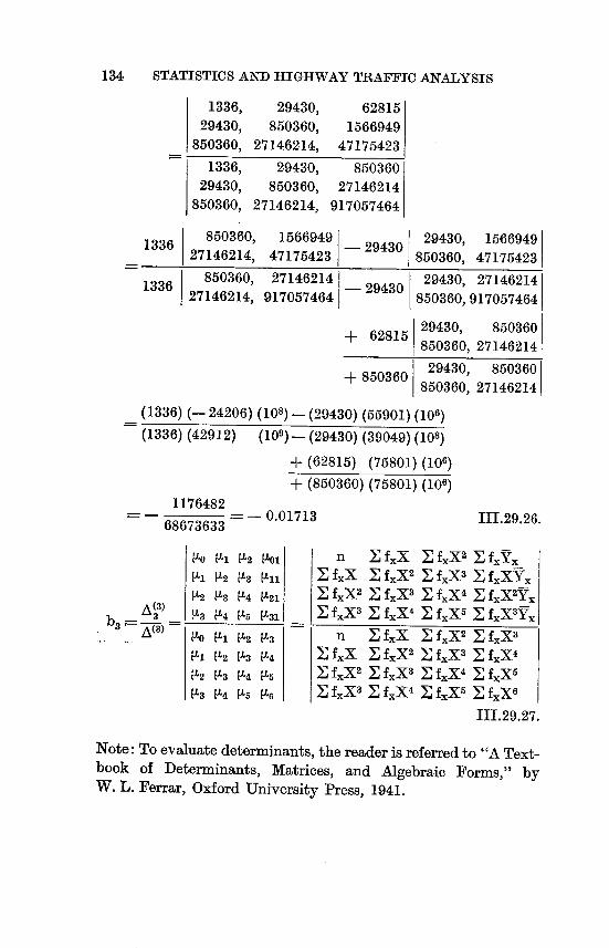
134 STATISTICS AND HIGHWAY TRAFFIC ANALYSIS
1336, 29430, 628151
29430, 850360, 15669491
860360, 27146214, 47175423
1336, 29430, 8503601
29430, 850360, 271462141
850360, 27146214, 9170574641
1336 850360, 15669491 - 29430 29430, 15669491 27146214, 471754231 850360, 47175423
1336 850360, 27146214 1 - 29430 29430, 27146214 127146214, 917057464 850360,917057464
+ 628115 29430, 850360 850360, 27146214
+ 850360 29430, 8503601 850360, 27146214i
(1336) (- 24206) (108) - (29430) (55901) (106)
(1336)(42912) (109) - (29430) (39049) (108)
+ (62815) (75801) (106)
+ (850360) (75801) (106)
1176482 = - 0.01713 II1.29.26. 68673633
['0 ILl [12 V01 n f.X 2: f.X2 fy.
tLl 112 113 I'll E fXX 1: f.X2 F , f.Y,3 fXXV. 112 t13 114 1421 fXX2 f.X3 f.X4 f.X2y.
(3) 1131 Y, fX3 fX4 fXX5 fX3y,bs L3 113 114 115 7-
A(3) fX fX2 fX3Ill k 113 n
Ill (12 IL3 k E f,,X f
X2 &X3 &X4
Z fX2 fXX3t2 IL3 114 [L5 fX4 fXX5
t3 114 115 t6 fX3 fXX4 fX5 fX6
111.29.27.
Note: To evaluate determinants, the reader is referred to "A Text
book of Determinants, Matrices, and Algebraic Forms," by
W. L. Ferrar, Oxford University Press, 1941.

135 STANDARD DISTRIBUTIONS
Next, it is necessary to obtain the various orthogonal polynomials. They are
n J&X 1336 2943011 X I X
n 1336 1
1336 X - 29430 X - 22.03 III.29.28.1336
n fX fX2fXX fXX2 &X3
P2 X X2 n f,,X &X &X2
EfXX fX21_Xl n E fxX2 + X2 n E f'X&X2 Z &X31 IEf,X E f',X3 f"X Z &X 2
n Y, f.X E f,,X E f_X2
29430 850360 1336 850360 + X2 1336 29430 1860360 27146214 X 29430 27146214 29430 850360
1336 29430 29430 850360
75800948420 - 11241247104 X + 269956060 X2
269956060 280.7899 - 41.6410 X + X2 III.29.29.
The linear regression (trend) function is
Y.'= bo + b, P, ;== bo + b, (X - 22.03) 47.017 + 0.909 (X - 22.03)
26.99 + 0.909 X III.29.30. which agrees with result obtained in III.23.2., p. 115 as it should.
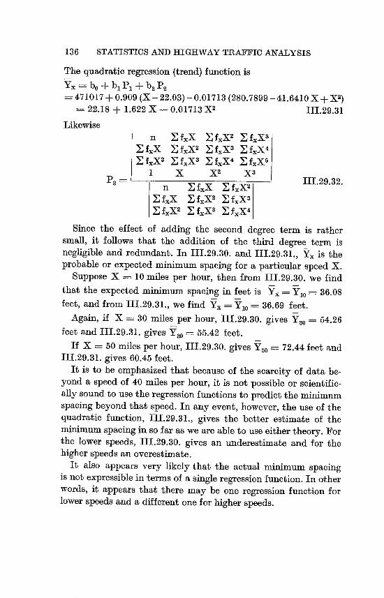
136 STATISTICS AND HIGHWAY TRAFFIC ANALYSIS
The quadratic regression (trend) function is
Y,, bo + b, PI + b, P2
471017 + 0.909 (X - 22.03) - 0.01713 (280.7899 - 41.6410 X + X2)
= 22.18 + 1.622 X - 0.01713 X2 III.29.31
Likewise n Z fXX Z fXX2 Z fX3
I fXX E fX2 Z &X3 Z fXX4
.E fX2 F, fX3 E fXX4 E fX5
X X2 X3 P3 n E f.X Z fXX2 III.29.32.
fXX 5, fXX2 'V fXX3 2.j
fX2 1: fX3 Y, fXX4
Since the effect of adding the second degree term is rather
small, it follows that the addition of the third degree term is
negligible and redundant. In III.29.30. and 111.29.31., Yx is the
probable or expected minimum spacing for a particular speed X.
Suppose X 10 miles per hour, then from III.29.30. we find
that the expected minimum spacing in feet is Yx = Y10 = 36.08
feet, and from III.29.31., we find YX Y10 = 36.69 feet.
Again, if X = 30 miles per hour, III.29.30. gives Y3o = 54.26
feet and III.29.31. gives Y30 = 55.42 feet.
If X = 50 miles per hour, III.29.30. gives Y50 72.44 feet and
III.29.31. gives 60.45 feet.
It is to be emphasized that because of the scarcity of data beyond a speed of 40 miles per hour, it is not possible or scientific
ally sound to use the regressionfunctions to predict the minimum
spacing beyond that speed. In any event, however, the use of the
quadratic function, III.29.31., gives the better estimate of the
minimum spacing in so far as we are able to use either theory. For
the lower speeds, III.29.30. gives an underestimate and for the
higher speeds an overestimate. TJLt also appears very likely that the actual minimum spacing
is not expressiblein terms of a single regressionfunction. In other
words, it appears that there may be one regression function for
lower speeds and a different one for higher speeds.

STANDARD DISTRIBUTIONS 137
REFErE,,TcEs, CEL&PTER III
Uspensky, J. V., "Introduction to Mathematical Probability," First Edition, McGraw-Hill Book Co., 1937, page 101.
2 Ibid., page 101. 3 Ibid., page 204. Tchebycheff, P. S., "Des Valeurs Moyennes," Journal de Mathematique
(2), Volume 12 (1867), pages 174-184. Bienayme, M., "Considerations a l'appui de la decouverte de Laplace Sur
la loi de probabilite dans la methode des moindres carres," Comptes Rendus, Vol. 37 (1853), pages 309-24.
4 Zoch, R., "On the Postulate, of the Arithmetic Mean," Annals of Mathematical Statistics, Vol. VI., No. 4, December 1935, pages 171-187.
Zoch, R., "Invariants and Covariants of Certain Frequency Curves," Annals of Mathematical Statistics, Vol. VI, No. 1, March 1935, pages 124-135.
5 Weida, F. M., "Maximum Term of Hypergeometric Series," American Mathematical Monthly, Vol. XXXIII, No. 6, June-July 1926, page 339.
6 Weida, F. M., "On Various Conceptions of Correlation," Annals of Mathematics, Second Series, Vol. 29, No. 3, July 1928, pages 276-312.
Rietz, H. L., "Mathematical Statistics," Open Court PublishingCo. 1927, pages 77-113.
Rietz, H. L., "Handbook ofMathematical Statistics," Houghton-Mifflin Co., 1924, pages 120-165.
1 Saculy, M., "Trend Analysis of Statistics," BrookingsInstitution, 1934, pages 33-37.
Kendall, M. G., "The Advanced Theory of Statistics," Charles Griffin and Co. Ltd., London, 1946, pages 145-152.
8 Rietz, H. L., "Mathematical Statistics," Open Court Publishing Co., 1927, pages 31-38.
9 Fry, Thornton G., "Probability and Its Engineering Uses," D. Van Nostrand Co., New York, 1928.
" Molina, E. C., "Poissons's Exponential Binomial Limits," D. Van Nostrand Co., New York, 1942.
11 Elderton,W. F., "Frequency Curves and Correlation," C. and E. Layton, London,1927.

CHAPTER IV
SAMPLING THEORY
Reliability and Significance
IV. 1. Objective. In this chapter it is proposed to show how to use the mathematicalmodels of distributionthat were developedin Chapter III as a basis for making inferences from a limitednumber of happenings that will apply to all such happenings. This process of reasoning from the particular to the general is known as inductive inference and in a broader sense is called 8ampling theory.
Inductive inference is a means by which scientific progress comes about. The research worker obtains data through planned experiments or through the observation of natural happenings such as the occurrence of accidents at certain types of highway intersections.From the data obtainedhe infers that certain things are so. But it is well known that exact inductive inference is theoretically impossible. One of the functions of statistics is to provide techniques for making inferences and for measuring the degree of certainty of the inferences.
In order to make the idea of inference somewhat more concrete, let us suppose that we have observed the speeds of one hundred vehicles at a given location and have found that five were traveling over seventy miles per hour. We might estimate from this sample that five per cent of all vehicles travel over seventy miles per hour, but we would not be very sure as to the correctness of our estimate for we know that a different sample of this limited size would undoubtedly lead to a different estimate. At best the sample contains but partial information about the law of behavior of the total population of drivers. Population is used in its statistical sense meaning a collection of results or objects. Summary numbers calculated from the sample accurately characterize the sample, but the important question is, how good are these same summary numbers when used as estimates of the characteristics of the population? What is the error committed by the use of
138

139 SAMPLING THEORY
sample characterizing numbers in place of the associated popula
tion characterizing numbers?
The role of statistics in providing a measure of the uncertainty
of inferences from samples is confined to sampling errors. It must
be assumedthat the experimenterhas guarded against accidents in
recording the data. In gathering data the first consideration is the
obtaining of a random sample.
IV. 2. Random Sampling: In order to demonstrate what is meant
by randomsampling let us supposethatwe have a given population
and that the attribute or attributes of the population to be mea
sured are specified. The problem is to find a sampling method for
the given population and the stochastic variable being measured
that will yield a randomor unbiased sample. The answer lies partly
in theory and partly in techniques that have been proven in
practice or may have to be devised to meet a given situation.
The first requirementis that there be no obvious connection be
tween the methodof selection and the properties being studied.The
method and the properties must be independent in so far as our prior knowledge enables us to make them so.
To meet the second requirement that the sample be a random
selection, we rely on our previous experience with a given method
as well as our intuition to justify its use on new occasions. A
very reliable method of drawing random samples consists of con
structing a model of the population and samplingfrom the model.
Actually, randomnessis largely a matter of intuition.The theory
of probabilityconsiders the set of all possibledifferentsamplesthat
may be drawn from a specified universe and enables us to derive
theirdistributionlawfor any desiredcharacterizing summary num
ber. This theoryrequires thatit be made certain that the sampling method will tend to yield all possibledifferent sampleswith equal
frequency. A method that does this is called a random method.
IV. 3. Distribution of Sample Arithmetic Means. For the purpose of illustrating the law of the distributionof sample arithmeticmeans,
let us suppose that we have a normal universe, and that from this
universe, we draw a large number of samples all of the same size,

140 STATISTICS AND HIGHWAY TRAFFIC ANALYSIS
n. If the samples are random and drawn independently, then the distributionof sample arithmetic means is also normal. Furthermore, the arithmetic mean of the distribution of sample arithmetic means is the true arithmetic mean of the universe and the standard deviation of the distributionof sample arithmeticmeans is the standard deviation of the universe divided by the square root of the size of the sample. Expressed symbolically: If X.,, X21
X31 ... I Xi' ... Xk are the sample arithmetic means and if X is the arithmetic mean of the universe from which the samples were drawn, then
- I Xi X - k IV.3.1.
If a is the standard deviation of the universe of measures and s-R is the standard deviation of the distribution of sample arithmetic means, then
a sX = -_ . IV.3.2.
yn The value R-x is frequently called the standard error of the arithmetic mean. Actually it is the measure of reliability of the arithmetic mean and is in fact the expected error committed when a particular sample arithmetic mean is used in place of the true arithmetic mean of the universe. The smaller the expected error, the more reliable or the more precise is the sample arithmeticmean.
The measure of reliability given by IV.3.2. is exact in theory but not usable in practice because the value of a depends upon the population which is not known. Consequently it is necessary to obtain from the sample an unbiased estimate of the universe variances, indicated by the symbol&2. This is equal to:
2 = S2 IV.3.3n - I
where S2 is the variance of the sample. Substituting this value a2
for r52in IV.3.2.. we obtain s
sx IV.3.4.
which is usable as the standard error of the arithmetic mean.

141 SAMPLING THEORY
It is to be noted that IV.3.3. gives an estimate of universe
variance.
Using the data of Table 11.1. it was found that the arithmetic
mean was 38.2 milesper hour and the standard deviation, 8.9 miles
per hour. In 11.22., page 50, it was also found that the expected
speed of 38.2 miles per hour was in error at most 23.3 per cent
with a measure of confidenceof 71 per cent. To find out how near
the true value of the arithmetic mean our sample mean is, we
substitute in IV.3.4. and find that
8.9 v = 0.52 Miles per hour. IV.3.5.
Vn- 1 299
which is the expected error in the sample arithmetic mean. In
other words, it is 68.27 per cent certain that the true arithmetic
mean in the universe has a value between 38.2 - 0.5 37.7 and
38.2 + 0.5 38.7 miles per hour. (68.27 is the per cent of area
contained within one standard deviation on each side of the
mean). In this case the maximum expected relative error is
0.52/38.7 1.3 per cent with 68.27 per cent certainty. In like
manner it is 95.45 per cent certain that the maximum relative
error does not exceed 2.6 per cent and similarlyit is 99.73 per cent
certain that the error does not exceed 3.9 per cent. The conclusion
then is that the sample arithmetic mean is fairly reliable (precise)
but as found before, it is not usable as a typical or characterizing
speed.
IV. 4. Inference Concerning Population -Mean. Let [i be the popu
lation mean and X the sample mean. It is desired to test the hypo
thesis: The sample whose mean is X could have come from a
population with mean ti. If this is so, how certain are we that
it did? This question is answered byusing the t-distributionwhere
in this case
t=1 X-[k I IVAJ.
Sx
For example: Could our sample with arithmetic mean of 38.2
miles per hour have come from a population whose arithmetic

142 STATISTICS AND HIGHWAY TRAFFIC ANALYSIS
mean is 40 miles per hour? Substituting the values already found
in IV. 4. I., we have
t 38.2 - 40.0 1.54
0.52
Making use of the t-table in "Statistical Methods for Research
Workers"5 with in this case n - I = 299 degrees of freedom it is
found that 5 per cent of the time the difference as expressed by t
would be at least 1.97. Only one degree of freedom is lost because
the only restriction is that the deviations are taken from the
mean of the sample. However, our value of t 1.54 is less than
1.97. Hence it is concluded that on the 5 per cent level of sig
nificance we have insufficient grounds to reject the hypothesis.
In other words, if the hypothesis is rejected, it would be rejected
when it is true slightly more than 5 per cent of the time. This
means that we would have a slightly greater than 5 per cent
risk in rejecting the hypothesis. To putit in another way the odds
are a bit less than 95 to a bit more than 5 per cent in favor of re
jection of the hypothesis. The level of significance and risk are synonymous, for the level of significance is the probability that
the hypothesis is true and its complement is the probabilitythat
the hypothesis is not true.
IV. 5. Confidence Limits. Since it is impossible to estimate or
predictthe true value exactlyit is necessary to obtain two numbers
between which the true value will fall. These two numbers are
known as confidence limits. To obtain them, it is necessary first
to determine the value of t associated with the relevant degrees
of freedom (number of possible values variable assumes minus
numberof rigorous conditionsor constraints the values must obey) and a desirable probability level of significance.
The sample arithmetic mean may be greater or less than the
populationarithmetic mean. From IV.4.1, it was found that
t

143 SAMPLING THEORY
It is not hard to see from this equationthat ---I- t = (X - [t)/s-, or
-4- ts- IV.5. I.
which gives the two values (confidence limits) between which the true sample arithmeticmean will fall. These values are based upon
the specific degrees of freedom and level of significance as de
manded by the subjective problem. The limit of significance and
the degree of reliabilitymay be of any desired value.
To illustrate: Suppose we have a sample whose arithmetic mean
is 52, whose standard deviation is 5 and whose size is 101. It is de
sired to find the confidence limits on a 5 per cent level.
Making use of the t-tablewith (n -1) =. 100 degrees of freedom
and IV.5. I., it is found that
52; 1.98 ( 5) 10
52 0.99
whence the two values of [t are 51.01 and 52.99.
This means that it is 95 per cent certain that the true arithmetic
mean of the universe lies between 51.01 and 52.99. Again, it is
95 per cent certain that if we take the arithmeticmean of 52 as the value of the population (true) arithmetic mean the error com
mitted will not exceed 0.99/52 .019 1.90 per cent. If the
error thatmay be tolerated (which is obtained fromthe subjective material) is not less than 1.90 per cent, then for the pertinent
purpose the sample arithmeticmean may be used asthe population
arithmetic mean. Otherwise, it may not be used.
IV. 6. Difference Between SampleArithmetic Means. Frequentlythe
arithmetic means are computed from two independent samples.
The question that needs to be answered is: Are these samples in
dependent and from the same normal universe? To answer this
question we again make use of the t-distribution, but in this case
we use for t the value V given by
I X1_ K21 1V.6.1.
V II(NI + NO (NI S2 + N2 S2)1 2
V (NI N2) (NI + N2 - 2)

144 STATISTICS AND HIGHWAY TRAFFIC ANALYSIS
where X, is the arithmetic mean of the first sample X2 is the arithmetic mean of the second sample 82
. is the variance of the first sample
281 is the variance of the second sample N, is the size of the first sample N2 is the size of the second sample N, + N2- 2 are the degrees of freedom and
(NI + NO (NI S21 + N2 '2 is the standard deviation of the V (NjN2) (Nj + N2- 2)
distributionof differences between independentsample arithmetic means from the same normal universe.
To illustrate: Suppose we have the following two samples:
Sample I Sample II
Arithmetic mean xi 145 i2 150 Standard Deviation SI_ 5 82 6
Number of Individuals N, 12 N2= 20
We wish to test the hypothesis: The difference between the sample arithmetic means is insignificant, therefore, these two samples are independent and from the same normal universe.
To make the test we use IV.6.1. Substituting the given values in IV.6.1., it is found that in numerical value
t/ 1145 - 1501 5 5 - - -- - = 2.35
1/32 [12 (25) + 20 (36)] 4.53 2.13 V 240 (30)
Making use of the t-table with (N,. + N2- 2) (12 + 20 - 2) = 30 degrees of freedom it is found that when t 2.042 the probability that the two samples came from the same normal universe is 0.05 and when t = 2.750 the probability is 0.01. The value of t = 2.35 lies between the 5 per cent and I per cent levels of signifioance, hence, we conclude that the two sample arithmetic means are significantly different on the 5 per cent level but not so on the 1 per cent level. This means that the odds are between 95 and
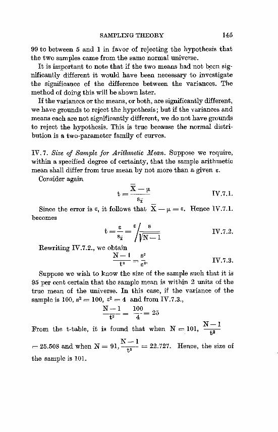
145 SAMPLING THEORY
99 to between 5 and I in favor of rejecting the hypothesis that
the two samples came from the same normal universe.
It is important to note that if the two means had not b'een sig
nificantly different it would have been necessary to investigate the significance of the difference between the variances. The
method of doing this will be shownlater.
If the variances or the means, or both, are significantly different,
we have groundsto reject the hypothesis; but if the variances and
means each are not significantly different, we do not have grounds
to reject the hypothesis. This is true because the normal distri
bution is a two-paxameter family of curves.
IV. 7. Size of Sample for Arithmetic Mean. Suppose we require,
within a specified degree of certainty, that the sample arithmetic mean shall differ from true mean by not more than a given e.
Consider again
t - X IV.7. 1. sx
Since the error is e, it follows that X - t Hence IV.7. 1. becomes
t= IV.7.2. B-X
Rewriting IV.7.2., we obtain N - I S2
_t2 2. IV.7.3.
Suppose we wish to know the size of the sample such that it is
95 per cent certain that the sample mean is within 2 units of the
true mean of the universe. In this case, if the variance of the
sample is 100, s2 = 100, S2 4 and from IV.7.3.,
N - I 100 t2
- 4 = 25
From the t-table, it is found that when N 101, N-1 t2
N - I 25.508 and when N = 91,
t2 22.727. Hence, the size of
the sample is 101.
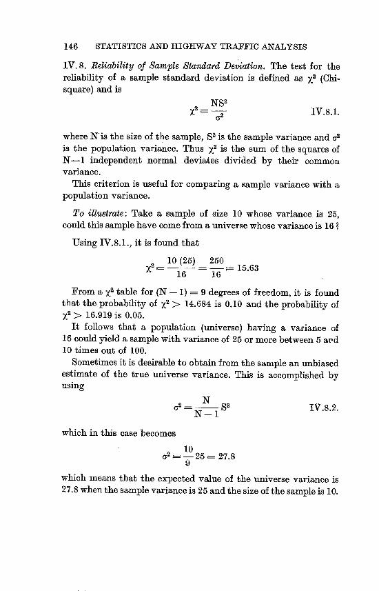
146 STATISTICS AND HIGHWAY TRAFFIC ANALYSIS
IV. 8. Reliability of Sample Standard Deviation. The test for the reliability of a sample standard deviation is defined as X2 (Chi-square) and is
2 NS2 Cy2 IV.8.1.
where Nis the size of the sample, S2 is the sample variance and e is the population variance. Thus X2 is the sum of the squares of N-1 independent normal deviates divided by their common variance.
This criterion is useful for comparing a sample variance with a population variance.
To illustrate: Take a sample of size 10 whose variance is 25, couldthis sample have come from a universe whose variance is 16
Using IV. 8. 1., it is found that
10 (25) 250- = - F-- 15.63 16 16
From a X2 table for (N - 1) = 9 degrees of freedom, it is found that the probability of X2 > 14.684 is 0.10 and the probability of
> 16.919 is 0.05. It follows that a population (universe) having a variance of
16 could yield a sample with variance of 25 or more between 5 avd 10 times out of 100.
Sometimesit is desirable to obtainfrom the sample an unbiased estimate of the true universe variance. This is accomplished by using
e= N S2 IV.8.2. N-1
which in this case becomes
10 a - 25 == 27.8
9
which means that the expected value of the universe variance is 27.8 when. the sample varianceis 25 and the size of the sampleis 10.

147 SAMPLING THEORY
IV. 9. Significance of Difference Between Sample, Varianm. The test here is to determine, with respect to variance, whether two
samples are independent and from the sample normal universe.
The criterion is the F-test which is given by
S' IV.9.1.S12 2
2NIS12 2 N2S2
where S - and S 2' - and the degrees of freedom N1- I N2_ 1
for S21 is N, - I and for S22
is N2 - 1. Having two unbiased esti
mates of variance, always usefor S12thegreaterof thetwo variances.I To illustrate: Let there be given two samples of 10 and 12 indi
viduals respectively. Let their variances be 10 and 5 respectively.
Are these two samples independent and from the same normal
universe? In other words, is the variance 10 significantly greater
than the variance 5?
Substitutingin IV. 9. 1., it is found that F becomes
F NIS12 / N2 S2
2 10 (10) 12 (5)
N1- I N2_ 1
2.04
From the F-tablewith n, = N3. - I = 9 degrees of freedom and
n2 = N2- I = 11 degrees of freedom, we find that at the 5 per cent level of significance F is 2.90 and at the I per cent level of significance F is 4.63.
Hence we conclude that, since our value of F is 2.04 which is less
than the F for the 5 per cent level, the larger varianceis not signi
ficantly greater than the smaller. In other words, there are not
sufficient grounds to reject the hypothesis that the two samples
could have come from the same normal universe.
IV. 10. Significance of a CorrelationCoefficient. The question here is:
Could the sample whose coefficient of correlation is r have come from a non-correlated universe? We use
t ON-2 IV.10.1.
VI _r2
where the degrees of freedom are N - 2.
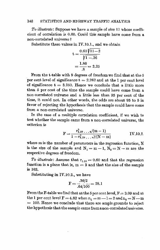
148 STATISTICS AND HIGHWAY TRAFFIC ANALYSIS
To illustrate: Suppose we have a sample of size II whose coefficient of correlation is 0.60. Could this sample have come from a non-correlated universe?
Substitutethese values in IV.10.1., and we obtain
t 0.60YII-2 VI -. 36
1.80 - = 2.25
.8 From the t-table with 9 degrees of freedomwe find that at the 5
per cent level of significance t = 2.262 and at the I per cent level of significance t 3.250. Hence we conclude that a little more than 5 per cent of the time the sample could have come from a non-correlateduniverse and a little less than 95 per cent of the time, it could not. In other words, the odds are about 95 to 5 in favor of rejecting the hypothesis that the sample could have come from a non-correlated universe. . In the case of a multiple correlation coefficient, if we wish to test whetherthe sample came from a non-correlated universe, the criterionis
2F_ ri. 23 . . . n/(M IV.10.2.
r21.2. .n)/(N m)
where m. is the number of parameters in the regressionfunction, N is the size of the sample and N, = m - 1, N2 N - m are the respective degrees of freedom.
To illustrate: Assume that r,.23 0.60 and that the regression function is a plane that is, m. = 3 and that the size of the sample is 103.
Substituting in IV. 10. 2., we have .36/2 28.1
.64/100
From theF-table we findthat atthe 5 per cent level, F = 3.09 and at the I per cent levelF = 4.82 when n, = m - 1 = 2 andn2=N-m
100. Hence we conclude that there are ample grounds to reject the hypothesisthatthe sample came from anon-correlateduniverse.

SAMPLrNG THEORY 149
To test the hypothesis concerning a partial correlation coefficient the procedure is the same as that for a simple correlation coefficient with the exception that the number of variables held constant must be substracted from the size of the sample N. Hence, if k-variables are held constant the test is
2 --- k__F r,2.34 ... n/1 IV. 103 .
kr,2.3-4./(N -k- 1)
REFERENCE, CHAPTER IV
Yule, G. Udney, and Kendall, M. C., "An Introduction to the Theory
of Statistics," C. Griffin & Co., London, 1937.
2 Croxton, F. E., and Cowden, D. J., "Applied General Statistics,"
Prentiss-Hall Inc., New York, 1946.
3 Rider, Paul, "Statistical Methods," John Wiley & Sons Inc., New York,
1939.
4 Kendall, M. C., "The, Advanced Theory of Statistics," Charles Griffin
& Co., London, 1946, Vol. I, page 40.
5 Fisher, R. A., "Statistical Methods for Research Workers," Oliver and
Boyd, Ltd., Edinburgh.
CHAPTER V
SOME APPLICATIONS OF
STATISTICAL METHODS
V. 1. Objective.This chapter illustrates some of the applications of
statisticalmethods to proble 'Ms of most interest to traffic engineers.
Usually a statisticalapproachismore, rationalthanany other and leads
to a better understanding of the factors involved. The methods
apply to all types of traffic problems, but firstwe shall study those
that have to do with highway capacity. These problems are of primary concern, for they are connected with the main purpose
of a highway which is to serve traffic.
V. 2. Confusion As to Meaning ofHighway Capacity. Before attempt
ing any analysis, it is necessary thatcertain termsbe defined. There
is some confusion as to what is meant by highway capacity. This
is brought out by the Highway Capacity Manuall, which states that the term perhaps most widely misunderstood and impro
perly used in the field of highway capacity is the word capacity
itself. Considerable work went into the preparation of this manual,
and it offers the most authentic and complete informationextant
on capacity. In Part 1, Definitions, is found the statement that
"the term capacity without modification, is simply a generic ex
pression pertaining to the ability of a roadway to accommodate
traffic." The manual gives three levels of capacity:
1. Basic Capacity: "The maximum number of passenger cars
that can pass a given point on a lane or roadway during one
hour under the most nearly ideal roadway and traffic con
ditions which can be attained."
2. Possible Capacity: "The maximum number of vehicles that
can pass a given point on a lane or roadway during one hour
under the prevailing roadway and traffic conditions."
3. Practical Capacity: "The maximum number of vehicles that
can pass a given point on a roadway or in a designated lane
150

151 APPLICATIONS OF STATISTICAL METHODS
during one hour without the traffic density being so great as
to arouse unreasonable delay, hazard, or traffic conditions."
Prevailing roadway conditions include roadway alignment,
number and width of lanes.
From a practical standpoint, speed should be included in any
definition of traffic capacity. The driver is interestedprimarily in
the amount of time it takes himto arrive at his destination.Perhaps
capacity, meaning vehicles per hour, should be supplementedby a
dimensionless index number similar to the Reynolds number in
hydraulics. This number would indicate critical limits.
Since the term capacity has a variable meaning, we shall in most
cases use the word volume and define it as the number of vehicles
passing a given point per unit of time. Density will refer to the
number of vehicles in a given length of lane. With these definitions
Average Volume Average Density times Average Speed.
V. 3. Theoretical Maximum Capacity (Volume). The amount of
traffic per unit of time depends on the speed and the spacing
between vehicles. The greater the speed the larger is the volume, and the greater the spacing the less is the volume. Therefore,
Volu__ - Speed Spacing
This same reasoning applies to any number of lanes in the same
direction, but with more than one lane, passing takes place, which
adds another factorto be considered. For the sake of simplicity,we
shall first take up the theoretical capacity of a single lane.
In general, anyone who has observed traffic knows that as
speeds increase, the spacing between vehicles increases. If the
spacing increases at a greater rate than the speed, then there is an
optimum speed that gives a maximum volume. If the spacing in
creases at a rate equal to or less than the speed, then the higher
the speed the greater the volume. The question of minimum spacingneeds to be examined critically.
The original assumption was that drivers should and did main
tain a'safe stopping distance behind the vehicle ahead. This safe
stopping distance was based on the possibilitythat the car ahead

152 STATISTICS AND HIGHWAY TRAFFIC ANALYSIS
might stop instantaneously. This, of course, practically never hap
pens for it can take place only through some unusual occurrence
such as the head-on collision of two vehicles. That the original
assumptionof minimum spacing persists is evidenced by an article
in Traffic Engineering for August, 1950, by Dr. Victor F. Hess, Physics Department, Fordham University, New York.2 It should
be mentioned that Dr. Hess is deriving a formula for safe travel
at a maximum efficiency. This article states accurately that the
stopping distance includes (1) a, the distance the vehicle travels
during the "reaction time", (time interval between the stop signal
observed and the instant the brakes are applied) and (2) b, the
distance the vehicle travels after the brakes are applied. The dis
tance a is proportionalto the speed of the car v.
a tv
Distance b, the braking distance, is the distance required to absorb the kinetic energy of the vehicle (1-/, MV2), and therefore
must vary with the square of the velocity; that is
b kV2
in which the constant k is a factor depending upon the efficiency of the brakes and the coefficient of friction between the tires and
the pavement. The stopping distance is equal to
a + b tv + kV2
in which t = reaction time, which is usually taken as .75 second.
V. 4. Stopping Distance And Minimum Spacing. Observations
have proved that the stopping distance is not the minimum spac
ingbetween vehicles.This fact may also be arrived at by inductive
reasoning.
If we assume that two vehicles are mechanically equivalentand
traveling at the same speed, then one can be stopped in the same
distance as the other, and if they both start to stop at the same
instant, they will come to rest at the same distance apart as when
the brakes were applied. The fact that the brakes cannot be
applied at the same time results from the rear driver's needing
time to react. What takes place is that the driver sees the car
ahead start to stop and then reacts and applies his brakes. This
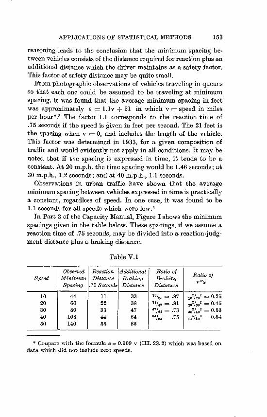
APPLICATIONS OF STATISTICAL METHODS 153
reasoning leads to the conclusion that the minimum spacing be
tween vehicles consists of the distancerequited for reactionplus an
additional distance which the driver maintains as a safety factor.
This factor of safety distance may be quite small.
From photographicobservations of vehicles traveling in queues
so that each one could be assumed to be traveling at minimum
spacing, it was found that the average minimum spacing in feet
was approximately s = I. 1v + 21 in which v speed in miles
per hour*.3 The factor 1.1 corresponds to the reaction time of
.75 seconds if the speed is given in feet per second. The 21 feet is
the spacing when v 0, and includes the length of the vehicle.
This factor was determined in 1933, for a given composition of
traffic and would evidently not apply in all conditions. It may be
noted that if the spacing is expressed in time, it tends to be a
constant. At 20 m.p.h. the time spacing would be 1.46 seconds; at
30 m.p.h., 1.2 seconds; and at 40 m.p.h., 1.1 seconds.
Observations in urban traffic have shown that the average minimum spacing between vehicles expressedin time is practically
a constant, regardless of speed. In one case, it was found to be 1.1 seconds for all speeds which were 10W.4
In Part 3 of the Capacity Manual, Figure I shows the minimum
spacings given in the table below. These spacings, if we assume a
reaction time of .75 seconds, may be divided into a reaction-judg
ment distance plus a braking distance.
Table V. I
Observed Reaction Additional Ratio of Ratio of Speed Minimum Distance Braking Braking V21S
Spacing .75 Seconds Distance Distances
10 44 11 33 33/3,, = .87 102 /202 = 0.25 20 60 22 38 38/47 = '81 20 2/3,2 = 0.45 30 80 33 47 47/64 = -73 302/402 = 0.56 40 108 44 64 14/85 = .75 40'/,502 = 0.64 50 140 55 85
Coupare, with the formula s = 0.909 v (III. 23.2) which was based on data which did not include zero speeds.
154 STATISTICS AND HIGHWAY TRAFFIC ANALYSIS
The braking distances for stopping shouldbe proportionalto the
square of the speeds, but as shown in the table, the minimum
spacings are not proportional to this amount. This is additional
evidence that minimum spacings do not depend on braking ability.
V. 5. Interpretation of Minimum Spacing Formula. The formula
s = 1. I v + 21 would give a maximum traffic flow of about 4000
vehicles per hour per lane. This, of course, is never realized except
momentarily. If a stream of traffic were moving at this minimum
spacing, the slowing or stopping of any vehicle would immediately affect all following vehicles. The formula is not given because of
its practicability but because it points to two significant facts.
a. The volume increases with speed, but apparently approaches
a maximum point at about 40 miles per hour where the con
stant 21 ceases to be significant.
b. The minimum spacing depends primarily on "reaction
perception-judgment" time.
V. 6. Limiting Factors. To summarize: The factors that limit the
capacity of a highway are:
I .Necessary minimum clearance between vehicles.
2. Slow moving vehicles that retard others, when passing is not
possible, due to lack of space on the opposite lane or to re
stricted sight distance.
3. Reduced overall speeds caused bythe physical features of the
highway, the mechanical characteristics of vehicles, or the
desire of drivers.
These factors need to be studiedin as much detail as possible if we
are to reach a clear conception of the problem of measuring the
ability of a highway to accommodate traffic.
V. 7. Additional Relationships of Spacing and Speed. In a study
made in Ohio in 1934 4 it was found that there is a straight line re
lationship between average density in vehicles per mile (spacing)
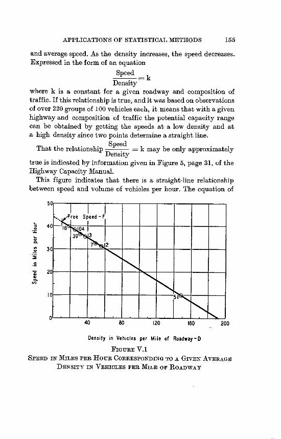
155 APPLICATIONS OF STATISTICAL METHODS
and average speed. As the density increases, the speed decreases. Expressed in the form of an equation
Speed
Density where k is a constant for a given roadway and composition of
traffic. If this relationship is true, and it was based on observations
of over 220 groups of 100 vehicles each, it means that with a given
highway and composition of traffic the potential capacity range can be obtained by getting the speeds at a low density and at
a high density since two points determine a straight line.
SpeedThat the relationship = k may be only approximately
Density
true is indicated by informationgiven in Figure 5, page 31, of the Highway Capacity Manual.
This figure indicates that there is a straight-line relationship
between speed and volume of vehicles per hour. The equation of
50 1 I ee Speed - F
0 4 4
39 3
0 3 2
20 WCL
An
0-
0 40 80 120 160 200
Den3ity in Vehicle3 per Mile of Roadway-D
FIGURE V. I
SPEED IN MILES PER HOUR CORRESPONDING TO A GivFN AvERAGE
DENSITY IN VEHICLES PER MILE OF ROADWAY

156 STATISTICS AND HIGHWAY TRAFFIC ANALYSIS
the curve for "the majority of existing highways" as nearly as may be judged from the Figure, is
S = 43 -. 009 V,
where S equals speed in miles per hour and V equals volumes
60
50
Ck
0 40
0-
201 0
1 2 4 6
1 8 10 12 14 16 18 20
Total Traffic (Hundreds)
Volume -Vehicles Per Hour
FIG7JRE V. 2AVERAGE SPEED OF ALL VEHICLES ON LEVEL, TANGENT SECTIONS
OF 2-LANE RURAL HIGHWAYS
(Figure 6, page 31, "Highway Capacity Manual", Used by Permissions of Bureau of Public Roads, U.S. Department of Commerce.)
LettingD . density in vehicles per mile of roadway, V = D -S, so that
S 43 -. 009 V 43 -. 009 D -S or
43 S 1+.009D
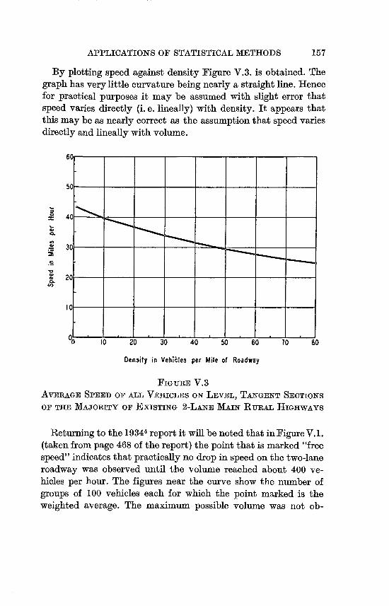
APPLICATIONS OF STATISTICAL METHODS 157
By plotting speed against density Figure V.3. is obtained. The
graph has very little curvature being nearly a straight line. Hence for practical purposes it may be assumed with slight error that
speed varies directly (i. e. lineally) with density. It appears that
this may be as nearly correct as the assumptionthat speed varies
directly and lineally with volume.
50
30
CX
10
10 20 30 40 so 60 70
Den3ity in Vehii:le3 per Mile of Roadway
FIGURE V.3
AVERAGE SPEED or, ALL VEHICLES ON LEVEL, TANGENT SECTIONS
OF THE MAJORITY OF EXISTING 2-LANE MAIN RuRAL HiGHwAys
Returning to the 19344 report it will be notedthat in FigureV.I.
(taken from page 468 of the report) the point that is marked "free
speed" indicates that practically no drop in speed on the two-lane
roadway was observed until the volume reached about 400 ve
hicles per hour. The figures near the curve show the number of
groups of 100 vehicles each for which the point marked is the
weighted average. The maximum possible volume was not ob

158 STATISTICS AND HIGHWAY TRAFFIC ANALYSIS
served directly, but was obtained by assuming that the curve was
a straight line. The "free speed" for the curve shown was 43.8
m.p.h. This point is indicated to be about ten units to the right
since no noticeable speed drop was observed until the volume
reached about 400 vehicles per hour. The maximum possible
volume would come at the mid-point of the curve and would equal
46 195 - X - 2,300 (approx.) vehiclesper hour. That the mid-point2 2
of the curve gives the maximum volume is easily proved.
Let S,,, = maximum speed and DM maximum density, then
Slope of SMDM
Let x=. varying values of D, then V S - X SM) x DM
SX X2
Differentiatingwith respect to x
dV S",- = S - 2 x dx DM
SM For maximum volume S - 2 x - = 0
DM
DMwhence, X - = midpointof the curve.
2
If this straight-line relationshipholds, then the maximum capacity
varies over a small range, since the end points of the line are fixed
by the maximum average speed and the minimum spacing which have small variations.
V. 8 Volume and Speed. If volume'is plotted against speed, the re-suiting curve is given m Figure VA. This curve shows that there
is a maximumvolume and also that there are two speeds that give
the same volume. At the lower speed, there is considerable time loss, Figure VA

159 APPLICATIONS OF STATISTICAL METHODS
50
Free Spe d- F
40
12
30
2 J-0
01Cn
51
'O 400 800 1200 1600 2000 2400 2800
Volume -Vehicles per Hour - V
FIGURE VASPEED IN MILES PER HOUR CORRESPONDING TO A GivEN VoLUmB
IN VEHICLES PER HOUR, ON A 2-LANE HIGHWAY
These curves bring out the fact that capacity needs to be ex
pressed in terms of both volume and speed. At maximum volume
there is always a considerable time or speed loss. The maximum
volume is evidently not a design volume.
The Capacity Manual gives a great deal of evidence that there
are definite relationships between speeds and volumes. This is
brought out by numerous curves which show such information as
the number of drivers desiring to pass compared to the number
that have an opportunityto pass, the total percentage of the time
that desired speeds can be maintained, and the point at which
drivers become influenced by the presence of vehicles ahead of
them. Using the facts set forth in the manual, it is our purpose to
see if there is a rationalexplanation of the interrelationshipsof the
different phases of the behavior of drivers that can be expressed
mathematically.

160 STATISTICS AND HIGHWAY TRAFFIC ANALYSIS
20
CL. 160
0 Nb
CL 120
0
80
_j 40
E 01 400 800 1200 1600 2000
L 2400 2800 3200
Volume - Vehicles per Hour - V
FIGURE V.5
VERICLE TimE Loss DUE TO CONGESTION ON A 2-LANE HiGHwAy
V. 9. The Nature of the Problems of Highway Traffic. We have discussed some of the elements of the problems of highway capacity, but have said very little about the nature and variability of these elements. It is this variabilitythat makes it difficult to solve the problems involved. If all vehicles traveled at the same speed, or if all people reacted in the same time interval, or if all drivers maintained the same spacing at the same speed, the solutions would be comparatively easy.
There is nothing new about the idea that the behavior pattern of drivers is a stochastic variable. One of the writers found in 1933, as already mentioned, that the minimum spacing depended primarily on reaction-timewhich psychologists have long recognized as a stochastic variable.3 Mr. John P. Kinzer assumed in 1934, that the traffic distribution on a roadway followed a "random" or Poisson distributions In England, Mr. William F. Adams found that free flowing traffic conformedso well to the distributiongiven

161 APPLICATIONS OF STATISTICAL METHODS
by a random series that it might be described as "normal." That
the time spacingsbetween vehicles follow a random series in urban
traffic was reaffirmed by a study made in 1944-46.7
V. 10. Spacing as a Random Series. The assumptionthat spacingin
either time or distance units follows the "random" series furnishes
a means of studyingthe nature of spacing. To satisfythe conditions
of the Poisson series, a roadway would have vehicles scattered
along it at random so that any vehicle would be completely in
dependent of any other vehicle, and equal segments of the road
would be equally likely to contain the same number of vehicles.
Granting that these conditions exist, the total number of vehicles
on a roadway divided by the number of segments of road equals
4 Cm" the average number of vehiclesper segment. Then, according
to the Poisson series, the probability of zero vehicles appearing in
a segment is
/Tno e -0!
The probability of one vehicle appearingis
-M /ml'\
The probability of two vehicles appearing is
/M2\
e -M T! )
and the probability of n vehicles appearing is
/M.\ e _n! )
The sum of all the individual probabilitiesis
/MO MI M2 m1a
e -a k-0! +-
I ! + -
2 1 + +-
n ! +
.... )

162 STATISTICS AND HIGHWAY TRAFFIC ANALYSIS
But am ml mu
em +_ +.....' -0! - I n!
Therefore,
e- -em = eO This simply demonstrateswhat we know, namely that the sum of all probabilities is unity, which means that an event is certain to
Table V.2
FITTING OF POISSON CURVE BY CHi-SQUARE TEST
NUMBER OF VEHICLES APPEARING IN FivE-MINUTE INTERVALS
Observations Taken on U.S. 20 Near Oaklawn, 1111nots. Data Supplied by the U.S. Public Roads. Administration.
1 2 3 4 5 6 7
0 4-?
t3 '0'z
1&71 Z' 0 4'
0 3 .009095 2.9831 -. 004 .000016 .000001, 1 14 .042748 14.021 J 2 30 .100457 32.949 -2.949 8.696601 .264 3 41 .157383 51.621 10.261 112.805641 2.185 4 61 .184925 60.655 .345 .110025 .002 5 69 .173830 57.016 11.984 143.616256 2.519 6 46 .136167 44.662 1.338 1.790244 .040 7 31 .091426 29.987 1.013 1.026169 .034 8 22 .053713 17.617 4.383 19.210689 1.090 9 8 .028050 9.2001
10 2 .013184 4.3241 -5.095 25.959 1.613 1 1 0 .005633 1.847 12 1 I .002206 1 .724 1 1 1
Chi-square, y2 = 7.747 m 4.75 seconds Degrees of Freedom = 9 - 2 = 7
163 APPLICATIONS OF STATISTICAL METHODS
happen or not to happen. In this case, it means that any segment is sure to contain zero or more vehicles since this covers all alternatives.
V. II - Test of Goodness of Fit of the Poisson Series. The goodness of fit of the Poisson Series to a set of data may be testedby the Chi-square (e) test. A cumulative Poisson table of probabilities is used to obtain the theoretical frequencies. The data in the illustrative example consist of the numbers of vehicles appearing in five minute intervals on Route U.S. 20 near Oaklawn, Illinois. The volume of flow averaged about II 5 vehicles per hour. These data were made available by the Public Roads Administration.
The first two columns in Table V.2. show the observed data. The figures in Column Three are taken from a Poisson table. Column Four is found by multiplying the figures in Column Three by the number of intervals observed (N = 328) to obtain the theoretical frequency. Column Five gives the differences between the observed or actual frequencies and the theoretical. Note that in this column the first two terms and the last four in Column Four have been combined to obtain a minimum actual or theoretical frequency that must be five or more. Column Six gives the square of these differences. The figures in Column Six divided by the theoretical frequency give the values in Column Seven. The sum of these values, 7.747, equals "Chi-square" (;2).
The degrees of freedom are equal to the number ofclasses less 2,
i. e., 9 - 2 =1 7. From a Chi-square table of probability levels, it is foundthat the probabilitylevel is about .60 or 60 per cent.
A .5 per cent level is usually taken as sufficient to indicate that there is reason to reject the hypothesis that the data can be represented by the curve. Therefore, the present level of about 60 per cent is taken to be rather conclusiveevidence that the data may be represented by the Poisson Curve.
V. 12. Test of Goodness of Fit of the Poisson Series to the Distribution of Spacings Between Vehicles. As already mentioned we are also interested in the distributionof the time or distance spacings between successive vehicles. It is these time-gaps on the opposite
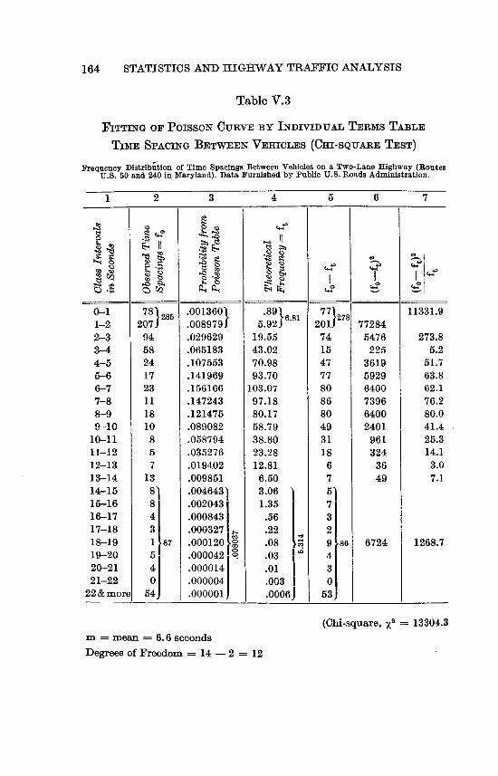
164 STATISTICS AND HIGHWAY TRAFFIC ANALYSIS
Table V. 3
FITTING OF POISSON CURVE BY INDIVIDUAL TERms TABLE
TmE SpAciNG BETWEEN VEMCLES (CHi-sQUARE TEST)
Frequency Distrib;ii1on of Time Spacings Between Vehicles on a Two-Lane Highway (RoutesU.S. 50 and 240 in Maryland). Data Furnished by Public U.S. Roads Administration.
1 2
0-1 781285 1-2 20 2-3 94 3-4 58 4-5 24 5-6 17 6-7 23 7-8 11 8-9 18 9-10 10
10-11 8 11-12 5 12-13 7 13-14 13 14-15 8' 15-16 8 16-17 4 17-18 3 18-19 187 19-20 5 20-21 4 21-22 0
22&morei 54
3 4 5 6 7
4f
4' tx
'0013601 5.891 17 127 11331.9 .008979 .92 6'81 201 8 772M .029629 19.55 74 5476 273.8 .065183 43-02 15 225 5.2 .107553 70-98 47 3619 51.7 .141969 93.70 77 5929 63.8 .156166 103.07 so 6400 62.1 .147243 97.18 86 7396 76.2 .121475 80.17 80 6400 80.0 .089082 58.79 49 2401 41.4 .058794 38.80 31 961 25.3 .035276 23.28 18 324 14.1 .019402 12.81 6 36 3.0 .009851 6.50 7 49 7.1 .004643 3.06 5 .002043 1.35 7 .000843 .56 3 .000327 .22 2 .000120 .08 9 86 6724 1268.7 .000042 'R .03 4 .000014 .01 3 .000004 .003 0 .000001 .0006 53
(Chi-square, X2 13304.3
m = mean = 6.6 seconds Degrees of Freedom = 14 - 2 12

165 APPLICATIONS OF STATISTICAL METHODS
lane that are used in passing. We shall now check the goodness of
fit of the time spacing distribution to the Poisson Curve. The data
were taken on Route U.S. 240, Maryland, and were furnished by
the PublicRoads Administration. The Chi-square testwill be used.
Accordingto this methodas showninTableV.3., it is immediately
evident that there is a wide discrepancy between the actual and
the theoreticalfrequencies. The probabilitylevel is practicallyzero.
If the distribution of time gaps between vehicles is not a Poisson
series, what is it? To determine this, let us re-examine the nature
of the Poisson series when applied to spacing distribution.
The probabilityof the occurrence of a time or distance gap of a given length is the probability that no vehicle will appear in the
given interval.
For example, given a volume of 400 vehicles per hour, let it be
required to determine the probability"Po" of a one second interval
having no vehicle. The average number of vehicles per second "m"
is equal to 4W/3100 ;:= 9' ; therefore, the probability of a one second interval having no vehicle is equal to
lmo -1 mo e-m 00 = e 0! )9
e`g, since 1 I (MO)! 1
The probability of no vehicle appearing in 2 seconds is e-5, and
in 3 seconds e-9'. In general, the probability Po of there being no
vehicles in "s" seconds is equal to e-m. This equation is of the
general form of y = ex
which may be written
lo& Y = x
therefore the equation when plotted on semilog-paper becomes a
straight line. The exponent, -m, means that the slope of the line
is negative. For plotting on semi-log paper we first arrange the data, as
shown in the cumulative Table VA. where the percentages of
spacings equal to or less than a given interval are tabulated.

166 STATISTICS AND HIGHWAY TRAFFIC ANALYSIS
Table VA
FITTING OF POISSON CURVE
EXPECTED ERROR METHOD
Class interv Class Cumulated Expected Expectedal Cumulated error or in seconds frequency frequency per cent natural error sn
(fo) uncertainty per cent
0-9 78 78 10.8 8.28 1.26 1-1.9 207 285 43.2 12.72 1.93 2-2.9 94 379 57.4 12.72 1.93 3-3.9 58 437 66.2 12.15 1.84 4-4.9 24 461 69.8 11.79 1.79 5-5.9 17 478 72.4 11.5 1.74 6-6.9 23 501 75.9 10.9 1.65 7-7.9 1 1 512 77.6 10.8 1.64 8-9.9 18 530 80.3 10.2 1.55
10-11.9 23 553 83.8 9.4 1.42 12-13.9 20 573 86.8 8.7 1.32 14-15.9 16 589 89.2 8.0 1.21 16-17.9 7 596 90.3 7.5 1.14 18-19.9 6 602 91.2 7.3 1.11 20-21.9 4 606 91.8 7.0 1.06 22-23.9 6 612 92.7 6.7 1.02 24-25.9 6 618 93.6 6.21 .94 26-30.9 10 628 95.1 5.47 .83 31-35.9 11 639 96.8 4.52 .68 36-40.9 8 647 98.0 3.89 .59 41-45.9 6 653 98.9 2.56 .39 46-50.9 1 654 99.1 2.56 .39 51-55.9 4 658 99.7 1.40 .21 56-60.9 0 668 99.7 1.40 .21 61-70.9 1 659 99.8 1.15 .17 71-80.9 1 660 100. 0 0
Mean = 4346.0 6.585 -R-0-
These percentages are represented by the heavy dots which fall in
an irregular line as shown in Fig. VA This is to be expected for
unless a sampleis very large thereis always a "naturaluncertainty"
or difference between the sample values and those of the universe.

100
APPLICATIONS OF STATISTICAL METHODS 167
50
m0.
C
5 Range of Expected Error (Natural Uncertainty)-
Cn
m
LO
Z LLI
CL
1.0
0.5
0.1 0 5 10 15 20 25 30 35 40 45 50 55 60 65
Spacing Beiween Successive Vehicles in Second3
FIGURE V.6
GRAPH SHOWING PERCENTAGE OF VEHICLE SPACINGS
AND TITE PROBABLE AmoUNTS OF THE "NAT-URAL UNCERTAINTY"
OF THE PLOTTED POINTS
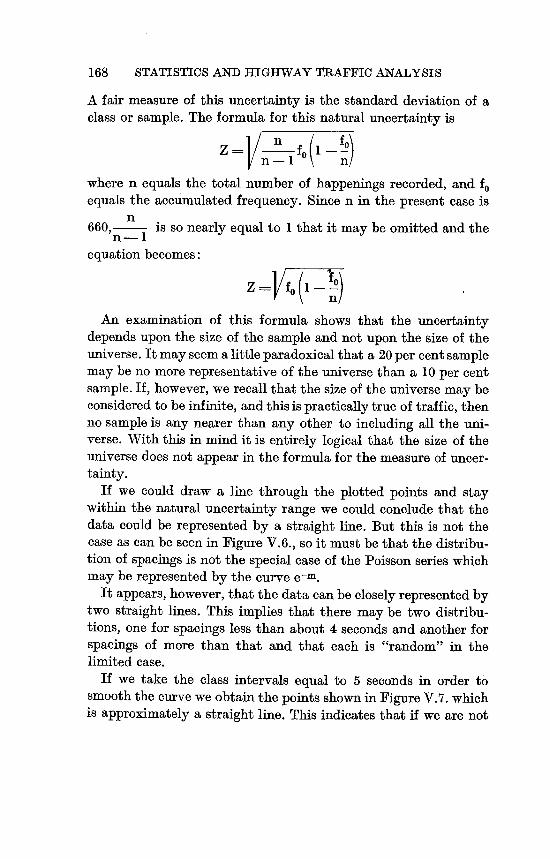
168 STATISTICS AND HIGHWAY TRAFFIC ANALYSIS
A fair measure of this uncertainty is the standard deviation of a class or sample. The formula for this natural uncertainty is
__fOI (I fo)_ n
where n equals the total number of happenings recorded, and fo equals the accumulatedfrequency. Since n in the present case is
n 660,_ is so nearly equal to I that it may be omitted and the
n-1 equation becomes:
Z = f 0 lnO))
An examination of this formula shows that the uncertainty depends upon the size of the sample and not upon the size of the universe. It may seem a littleparadoxical that a 20 per cent sample may be no more representative of the universe than a 10 per cent sample. If, however, we recall that the size of the universe may be consideredto be infinite, and this is practicallytrue of traffic, then no sample is any nearer than any other to including all the universe. With this in mind it is entirely logical that the size of the universe does not appear in the formula for the measure of uncertainty.
If we could draw a line through the plotted points and stay within the natural uncertainty range we could conclude that the data could be represented by a straight line. But this is not the case as can be seen in Figure V.6., so it must be that the distribution of spacings is not the special case of the Poisson series which may be represented by the curve e--.
It appears, however, that the data can be closely represented by two straight lines. This implies that there may be two distributions, one for spacings less than about 4 seconds and another for spacings of more than that and that each is "random" in the limited case.
If we take the class intervals equal to 5 seconds in order to smooththe curve we obtain the points shown in Figure V.7. which is approximately a straight line. This indicates that if we are not

169 PPLICATIONS OF STATISTICAL METHODS
100
5040
CL 30
20
co F
lo
5 La
4
3
0 5 10 15 20 25 30 35 40 45 50 55
Spacing Between Successive Vehicles in Seconds
A
FIGUREV.7
DISTRIBUTION OF SPACINGS BETWEEN SUCCESSIVE VEHICLES:
CLASS 11,TTERvALs EQUAL TO 5 SECONDS
concerned with spacings of less than 5 seconds that the straight line represents the distribution of the spacings closely enough for approximate analysis.
V. 13. Xinimum Spacing. For what is believed to be thefirst indicationthat minimumspacingdistributionsmight be different from
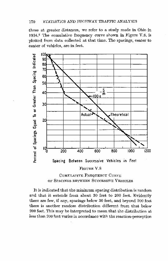
170 STATISTICS AND HIGHWAY TRAFFIC ANALYSIS
those at greater distances, we refer to a study made in Ohio in
1934.5 The cumulative frequency curve shown in Figure V.8. is
plotted from data collected at that time. The spacings, center to
center of vehicles, are in feet.
100 908070
A N'60
50
S- 40 10 e M4!W 30
0Actua I ̀ *N ,N T eoretical
20
CL
In 'O 200 400 600 800 1000 1200
Spacing Between Successive Vehicles in Feet
FIGURE V. 8
CumULATivE FREQUENCY CURVE
OF SPACINGS BETWEEN SUCCESSIVE VEHICLES
It is indicatedthat the minimum spacing distributionis random
and that it extends from about 30 feet to 200 feet. Evidently
there are few, if any, spacings below 30 feet, and beyond 200 feet there is another random distribution different from that below
200 feet. This may be interpreted to mean that the distribution at
less than 200 feet varies in accordance with the reaction-perception

171
100
50 40
CL 10 30
I 0
'1000
5
4
3
2
0 6, 1 14, 1,6 1 0
Time Spacing Between Successive Vehicles in Seconds
APPLICATIONS OF STATISTICAL METHODS
time of the driver and his judgment of what constitutes a safe
distance. Beyond 200 feet, the spacing may be judged to be in
accordance with the chance placement of the vehicles on the high
way. If the observed results are compared with the theoretical
FiGURE V.9
CUMULATivE FREQ7UENCY GURVE OF SPACINGS 13ETWEEN SUCCES
SIVE VEHICLES FOR VARio-us TRAFFIC VOL-UMES ON A TYPwAL
2-LANE RuRAL HIGHWAY
curve, it is found that the deviations from the random distribution
are accounted for by there being:
(a) No spacings below 30 feet.
(b) An excess of spacings between 30 and 200 feet.
(c) A deficit of spacings in excess of 200 feet.

172 STATISTICS AND HIGHWAY TRAFFIC ANALYSIS
These discrepancies are logical, for the minimum spacing, center to center of vehicles, is limited by the length of the vehicles and because vehicles, closing up behind slower vehicles must wait for an opportunity to pass, create a preponderance ofthe smaller spacings.
If the spacing of about 200 feet is divided by the average speed of 34.1 miles per hour we obtain about 4 seconds as the limit of the zone of speeds reduced by the presence of other vehicles. These data from twolocations, would not be supposedto give a conclusive answer.
For more extensive data, let us turn to Figure 9, page 40 of the Capacity Xanual. These data replotted as nearly as is possible from the printed curves are shown in Figure V.9. They are in time spacings and the breaks in the curves seem to come between five and six seconds.
Theoretically, if the lines had no breaks there would be no interference, and if all vehicleswere restricted there would be no breaks. These conditions were found and reported in the earlier paper referred to. To find the average of the "influenced" spacings we first make the reasonable assumption from the graphs that practically no spacings are under/2 second or over 6 seconds, and draw a line between these points as in Figure V. IO. This line then represents a random distribution of "influenced" spacings.
The next step is to let S m, where m is the average spacing. Now the expression
100 ( -iii-) =100 (e 0.368 36.8%
so that the average wouldbe at point36.8 per cent and wouldequal about 1.7 seconds. At this average "random" spacing all vehicles would be travelling at a restricted speed due to the closeness of spacing betweenvehicles.
V. 14. The Xinimum Spacing qt Four-Lane Traffic: Traffic on a four-lane highway does not have the same spacingrestrictions as a two-lane roadway. Vehicles are free to weave into the adjoining lane. When the curves shown in Figure 10, page 41 of the Capacity

173
100
CL
50 40
30 C
Cn 20
C
0 100e
5
4
3
2 -C;
0. 10, 2 3 4 '6'
Time Sgacing Between Successive Vehicles in Seconds
FIGURE V. 10
APPLICATIONS OF STATISTICAL METHODS
RANDom DISTRIBUTION OF "INFLUENCED" SPACINGS
Manual are replotted as shown in Figure V.11., the resulting curves show no breaks. The distribution of timespacingsis evidently random throughout.
V. 15. Frequency Di8tribution of Speed8: Having determined the characteristics of the spacing distributions, the next step is that of determiningthe nature of the distributionof automobile speeds.

174 STATISTICS AND HIGHWAY TRAFFIC ANALYSIS
100
50403 200
20
CLCn
10 r_co
WA
3
la 2
U0
CL
0.5CA 04M. 0.3
0.2
0.16 4 8 12 16 20 24 28
Time Spacing Befween Successive Vehicles in Seconds
FIGURE V.11
CumULATivE FREQUENCY CURVE OF SPACINGS BETWEEN SUC
CESSIVE VEHICLES FOR VARIOUS TRAFFIC VOLUMES ON A TYPICAL 4-LANE RURAL HIGHWAY
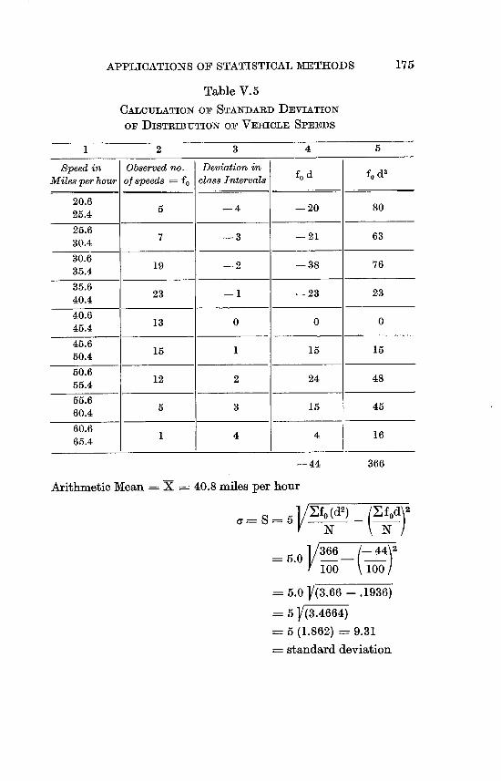
175 APPLICATIONS OF STATISTICAL METHODS
Table V. 5
CALCULATION OF STANDARD DEVIATION
OF DISTRIBUTION OF VEMCLE SPEEDS
2 3 4 5
Speed in Observed no. Miles per hour of speeds fo
206 5 25.4
25.6 30.4 7
30.6 35.4 1 9
35.6 40.4 23
40.6 45.4 1 3
45.6 50.4 1 5
50.6 55.4 12
55.6 560.4
60.6 65.4 1
Arithmetic Mean X
Deviation in f, d fo d2
class Intervals
- 4 - 20 80
- 3 - 21 63
- 2 -38 76
- I - 23 23
0 0 0
1 1 5 1 5
2 24 48
3 1 5 45
4 4 1 6
- 44 366
40.8 miles per hour
]/Zfo(d2) tZfdp5 V N
1/3f66_ -n44)2 'In fj
100 100
5.0 V(3.66 -. 1936)
5 r(3.4664)
5 (1.862) = 9.31
standard deviation
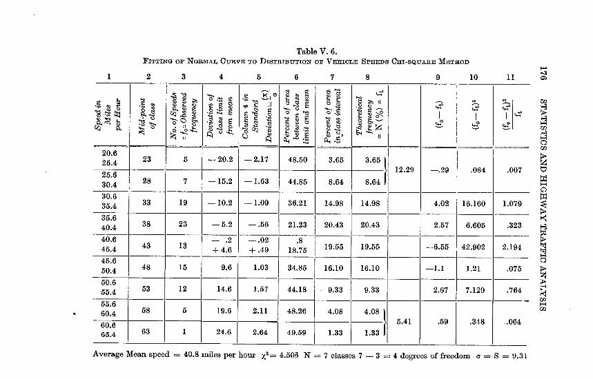
Table V. 6. FiTTING OF NORMAL CuRvE To DiSTRIBUTION OF VEHICLE SPEEDS 0111-SQUARE METHOD
1 2 3 4 5 6 7 8 9 10 1 1
9r.3
4:
4' 4'
EN Z,
20.6 25.4 23 5 - 20.2 - 2. 17 48.50 3.65 3.65
25.6 - 1 12.29 -. 29 .084 .007 30.4 28 7 - 15.2 - 1.63 44.85 8.64 8.64
30.6 35.4 33 19 - 10.2 - 1.09 36.21 14.98 14.98 4.02 16.160 1.079
35.6 40.4 38 23 - 5.2 -. 56 21.23 20.43 20.43 2.57 6.605 .323
40.6 45.4 43 13
- 2 + 4.6
-. 02 + .49
.8 18.75 19.55 19.55 -6.55 42.902 2.194
45.6 50.4 48 15 9.6 1.03 34.85 16.10 16.10 -1.1 1.21 .075
50.6 55.4 53 12 14.6 1.57 44.18 9.33 9.33 2.67 7.129 .764
55.6 60.4 58 5 19.6 2.11 48.26 4.08 4.08
5.41 .59 .348 .064 60.665.4 63 1 24.6 2.64 49.59 1.33 1.33
Average Mean speed = 40.8 miles per hour X.2= 4.506 N7 classes 7 - 3 4 degrees of freedom cr S = 9.31
177 APPLICATIONS OF STATISTICAL METHODS
It has been found that this distribution closely follows the
normal curve." Again as in the two previous examples of "ran
dom" distribution, the usual method of makinga test of the good
ness of fit is the Chi-Square (Z2) test. For the sake of simplicity,
let us take a small sample of 100 recorded speeds. The area method
of fitting a normal curve to the observed distributionwill be used.
The area includedwithin any number of standard deviations may
be obtained from prepared tables of areas of the normal curve. The
calculation of the standard deviation is shown in Table V.5.
The steps in the calculationare arranged as shown in Table V. 6., with the data in the respective columns consistingof the following:
(1) The speeds in class intervals of 5 miles per hour.
(2) The mid-points of the classes.
(3) The number of speeds recorded, i. e. the frequency fo.
(4) The deviations of the class limits from the arithmetic mean.
(5) The deviations from the mean in terms of standard devia
tions. This column is obtained by dividing the numbers in
column 4 by the standard deviation.
(6) Per cent of the area between the class limit and the mean.
This is obtained from an area table of the normal distribu
tion.
(7) Per cent of area in class interval. This is obtained by sub
tracting successivelythe numbersin column 6.
(8) The theoretical frequency ft is obtained by multiplyingthe
per cent of area in each class interval by the total number
of speeds observed. This equals 100 in the present case.
(9) This column gives the difference between the observed fre
quency fo (column 3) and the theoretical frequency ft
(column 8).
(10) This column is obtained by squaring the items in column 9.
(I 1) The sum of the items in this column equals ). This is the
value we use with the Chi-square table.
In using the chi-square table we need to know the degrees of
freedom. In fitting a normal distribution three degrees of freedom
are lost (or three constraints are imposed) because (1) the total
frequency, (2) the arithmetic mean, and (3) the value of the
178 STATISTICS AND HIGHWAY TRAFFIC ANALYSIS
standard deviation are used in computing the normal frequencies. The possible number of degrees of freedom is equal to the number of class intervals, 7 in this case. Therefore, 7 - 3 = 4, the degrees of freedom in the given example.
We find from the Chi-square table that the probability level is more than 5 per cent which means that in more than 5 times out of 100 the sample could have comefrom the universe tested. This level of 5 per cent is taken to mean that there is not sufficientevidence to reject the hypothesisthat the data can be representedby a normal curve. In the present case the probability is more than .30 which means that a variation as great as the amount found might occur in 30 cases out of 100 due to chance. Therefore it is not to be considered as significant.
V. 16. A Graphical Method of Determining Goodne88 of Fit. Another means of determining whether the distributionis normal or not is to plot the percentage of speeds at or less than various speeds on arithmetic probability paper. If the distribution is "normal" the observeddata will be represented by a straightline. In such a case, due to symmetrythe speedgiven bythe intersectionof the straight line with the 50 per cent ordinateis the most frequent and average speed, as well as the median. The usual definitions become:
Mean Average Speed arithmetical mean of all speeds - also called probable or expected speed.
Median Speed= speed such that 50 per cent of the speeds are greater, and 50 per cent less.
Modal Speed the most frequently occurring speed. The datautilized are the numbers of cars withspeeds equal to or
less thana given series of equallyspacedvalues. The same data will be used as in the first illustration. It is shown in Table V.7.
The points listed in Table V.7. are plotted in Figure V.12. It will be seen that they fall in rather irregular fashion, and that at first glance- the position of the 63.5 mile per hour point appears to preclude the possibilityof drawing a satisfactorystraight line.

179 APPLICATIONS OF STATISTICAL METHODS
0
80
t 50 -00 40
3
.01 0.1 0.5 I 2 5 10 20 30 40 50 90 95 9B 99 998 9999
Percent of Total Vehicle3, Traveling At Or Below Speed3 Indicated
FIGURE V. 12
GRAPH SHOWING PERCENTAGE OF VEHICLES TRAvELING ABovE
AND BELOW VARIOUS SPEEDS AND THE PROBABLE AmoU-NTS OF
THE "NATURAL UNCERTAINTY" OF THE PLOTTED POINTS
Table V.7
Speed in Miles Cumulated Percent Equal Natural
Per Hour Frequency to or Slower Uncertaintyin Percent
20.5 0 0 0.0
25.5 5 5 2.18
30.5 12 12 3.24
35.5 31 31 4.62
40.5 54 54 4.97
45.5 67 67 4.70
50.5 82 82 3.84
55.5 94 94 2.37
60.5 99 99 0.99
63.5 100 100 0.0
65.5 100 I 100 0.0

180 STATISTICS AND HIGHWAY TRAFFIC ANALYSIS
First, however, it is importantto considerthe probable amounts of the "natural uncertainty". Recall that the natural uncertainty
f Z +41 -_O . This natural uncertainty is given for each fre
n) quency in the last column of the table.
If the percentage of cars travelling slower than a given speed or equal to it is plotted against speed, the points will fall in an irregularline. This is to be expected, particularly when the number of cars represented in one diagramis only 100. If counts are made a number of times under precisely the same conditions of traffic, the percentage traveling faster than, say 40 miles per hour, will never be exactly the same, except by chance. There will be a certain dispersion around the average value for several groups of 100 cars. This we have already referred to in article V.12. as a Ccnatural uncertainty".
Through eachplotted point, a horizontalline is drawn representing the allowed ± range in the value of fo. It is then permissible to draw a smoothed curve in such a way that it passes through all the horizontal lines, attempting to draw it so that the sum of the deviations from the actually counted values shall be equal.
In the present case, a straight line satisfies all but the 63.5 mile per hour point. In the preceeding formula, fo should really be the mean number of cars with velocity equal to or less than the given amount, found from a great number of sets of 100 cars under the same traffic conditions. In such cases, it is fair to suppose that an occasional car traveling faster than 63.5 miles per hour would be found. Then the actual percentage slower than 63.5 would be slightly less than 100. If, for example, it were 99.5, the natural uncertainty would then be ± 0.7, and the point and the dotted line would give the result. In this case, it is evident that the straight line can be passed through all the horizontal lines. This means principally, that the points given by the higher speeds are too erratic and sensitive to accidental fluctuations to be given much weight in drawing of the curve. Probably all points for percentages less than 2 and greater than 98 should be ignored in drawing the curve.
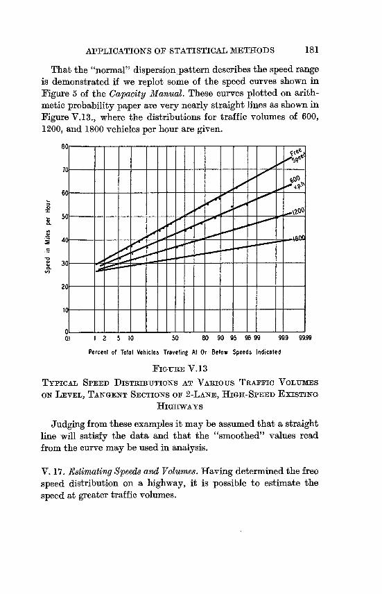
181 APPLICATIONS OF STATISTICAL METHODS
That the "normal" dispersion.pattern describes the speed range
is demonstrated if we replot some of the speed curves shown in
Figure 5 of the Capacity Manual. These curves plotted on arith
metic probability paper are very nearly straight lines as shown in
Figure V.13., where the distributions for traffic volumes of 600,
1200, and 1800 vehicles per hour are given.
70 00 0000 0000,
60
.000 Ole
o,,o40
ol
30
I 0- - ----
a] 12 5 10 50 80 90 95 98 99 99.9 99.99
Percent of Total Vehicle3 Traveling At Or Below Speed5 Indicated
FIGURE V. 13
TYPicAL SPEED DISTRIBUTIONS AT VARio-us TRAFFic VOLUMES
ON LEVEL, TANGENT SECTIONS OF 2-LANE, HIGH-SPEED EXISTING
HIGHWAYS
Judging from these examplesit may be assumed that a straight
line will satisfy the data and that the "smoothed" values read
from the curve may be used in analysis.
V. 17. Estimating Speeds and Volumes. Having determinedthe freo
speed distribution on a highway, it is possible to estimate the
speed at greater traffic volumes.

70
60
50 ge of hher speed vehicles
40 3 era lowerIgel Of speed veh cles
30
on Majority 20 in Highways
.6
1 5 10 20 50 70 90 95 98 99 99.9 99.99
Percent of Total Vehicles Traveling At Or Below Speeds Indicated
182 STATISTICS AND HIGHWAY TRAFFIC ANALYSIS
The first step is to find the average difference in speed between the vehicles being passed and the passing vehicles. The rate at which the faster vehicles are overtaking the slower ones can be found from a speed distributioncurve.(') Such a curve is shown in Figure V. 14. as replotted from Figure 4, page 30, of the Capacity
FIGURE V. 14
FREQUENCY DISTRIBUTION OF TRAVEL SPEEDS OF FREE MOVINGVEHICLES oiT LEVEL, TANGENT SECTIONS OF THE MAJORITY OF
EXISTING 2-LA-,NTE MAIN RURAL HIGHWAYS
Manual. It is evident that there are just as many vehicles traveling above the average (or 50 percentile speed) as below it. The average speed differential is the difference between the average speed of the 50 per cent faster vehicles and the 50 per cent slower vehicles. The average of the 50 per cent faster vehicles comes at the 78.75 percentile, and the average of the 50 per cent slower vehicles comes at the 21.25 percentile.(')
(a) In a study of passing made in 19356, it was found that vehicles in the act of passing other slower vehicles were traveling 9 to 10 miles per I- ur faster. The Capacity Alanual gives 9.6 miles as the average passing speed differential. (Footnote continuedon p. 183).
(b) This can be proved as follows: Let Figure V. 15 represent the same curve as Figure V. 14., but plotted on linear cross section paper.

183 APPLICATIONS OF STATISTICAL METHODS
The average speed of the faster vehicles equals 47.5 miles per
hour and the average for the slower ones is 37.5 miles per hour, so
that the average difference is 10 miles per hour.
Y
X&Y=,,lTri7 e-WV
YX
dx
FIGURE V. 15
DETERMINATION OF THE MEAN ABSCISSA OF THE UPPER HALF OF THE NORmAL DISTRIBUTION CURVE AND THE AREA TO THE RIGHT
OF THIS ABSCISSA
Required: To find (1) the mean abscissa of the upper half of the normal distribution curve, and (2) the area to the right of this abscissa.
X'y dx = 2fo"o xy dx
2 foo - x2 - xe -2--- dxf2 --
Y2- cr, which is about = .798 a. 77
From a table of areas under the normal curve, the area to the right of .798 a is .2125, or 21.25 per cent of the total area. In other words, 21.25% of the speeds will exceed the average of all the speeds higher than the average speed. Similarly, because of symmetry, 21.25% of the speeds less than the average will be less than the average of all the speeds lower than the average speed.
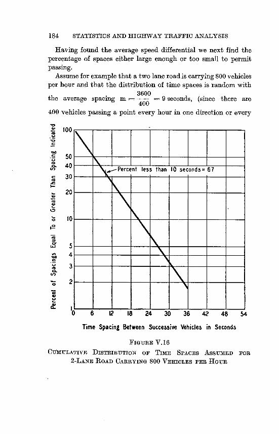
184 STATISTICS AND HIGHWAY TRAFFIC ANALYSIS
Having found the average speed differential we next find the percentage of spaces either large enough or too small to permit passing.
Assume for example that a two lane road is carrying800 vehicles per hour and that the distribution of time spaces is random with
3600 the average spacing m = - = 9 seconds, (since there are
400
400 vehicles passing a point every hour in one direction or every
100
so
40 Perc nt less than 10 seconds= 6730co
20
10
Z
IffV) 4uo
3C1.
2
0 6 12 18 24 30 36 48 54
Time Spacing Between Successive Vehicles in Seconds
FIGURE V. 16CumuLkmvE DISTRIBUTION OF TimE SpAcEs ASSUMED FOR
2-LANE ROAD CARRYING 800 VEHICLES PER HOUR
APPLICATIONS OF STATISTICAL METHODS 185
3600 seconds) and that the minimum spacing is 1/2 second. The
curve for the distributionis shown in Figure V.16.
WithlOsecondsastheaveragetimerequiredforpassingwefind from curve V. 16. that 67 per cent of the spaces are too small for
passing. This means that 67 per cent of the time a driver on this
highway could not pass because of vehicles on the opposite lane.
This concept becomes clear if we keep in mind that at any
instant the chance of there being a space of less than 10 seconds
of free space on the oppositelane is equal to the percentage of the total spaces that are less than 10 seconds. In this sense the size of
the time-gap has nothing to do with the chance of its being oppo
site the driver at any particular instant. It is only the frequency of
the occurrence of the space that determines the probability of its
happening in so far as passing is concerned. This reasoning becomes clearer if we remember that a space even if large is usually
used for onlyone passing. For example 6 time spaces might occupy
50 seconds with one equal to 10 seconds to permit one passing or
one of the spaces might be 25 seconds and still permit only one
passing during the 50 seconds. (See Article V.23 for mathematical
solution.) If a driver is not to be retarded,he mustevery time he approaches
a vehicle ahead, immediately pass the leading vehicle. If his speed
is on the average IO miles an hour faster, then that per cent of the
time he cannot pass is the per cent of the 10 miles per hour differ
ence that he mustlose. In the presentinstance he would lose 67 per
cent of 10 miles per hour or 6.7 miles per hour. Subtracting this
fromthe 43 miles per hour average speed gives 36.3 miles per hour
as the estimated average speed if the volume is 800 vehicles per
hour for two lanes. This very -nearly equals the observed speed of
36 miles per hour as shown in the lower curve, Figure 5, page 31,
of the CapacityManual. This resultwouldindicate thatthis method
of estimating is accurate enough to give good design figures. As a
further check let us estimate the speed for 1200 vehicles per hour
for two lanes. From the curve shown in Figure V. 17. we find that
vehicles are prevented from passing for 83 per cent of the time.
The speed drop is thus 83 per cent of 10 miles per hour = 8.3
miles per hour. Subtracting this from 43 = 34.7. This is more than

186 STATISTICS AND HIGHWAY TRAFFIC ANALYSIS
100
50 CL
40 verage= Seconds
30
20
0 10
ti
UJ 5
4
M 3CL
2
Q. '0' 6 12, 18 24 30 36 42 48 54
Time Spacing Beiween Successive Vehicles in Seconds
FIGUREV. 17
CUMULATIVF, DISTRIBUTION OF TimE SPACES ASSUMED FOP.
2-LANEROAD CARRYING 120OVEHICLES PERHoUR
the observed results of about 32 miles per hour shown in Figure 5, page 31, of the Manual.
This lack of agreement needs to be examined to see if there is an explanation. According to the theoryjust advancedthe speed drop dueto inabilityto pass cannotexceedthe average speed differential. How can we account for a speed drop greater than this ? The logical conclusionis that a further speed drop is not dueto an inability to

187 APPLICATIONS OF STATISTICAL METHODS
pass but to some other cause. If we recall that there is a speed drop
directly proportional to spacing the reason for the further speed
loss becomes clear. With a volume of 1200 vehicles per hour, a
high percentage of vehicles are traveling in the six second zone of
mutual interference and are slowed because they are too close to
gether rather than because of an inabilityto pass.
V. 1S. Estimate of Size Gap Required for Weaving. It is impossibleto
estimate the speed drop for a given increase in volume on a four-
lane road without knowingthe time-gap requiredfor weaving. But
since the speed drop has been measured, it is possible, by reversing
the method just explained, to estimate the time-gap for weaving.
From Figure 46, page 122, of the Capacity Manual, we find that
at 1700 vehicles per hour, the distributionbetween lanes is equal.
The speed on both lanes at thispointshould be the same. Referring
to Figure 7, page 33, ofthe CapacityManual, the speed at a flow of
1700 vehicles per hour is about 41 miles per hour. This is a drop of 7 miles per hour. Since the average speed differentialis 8.8 miles per
hour, in order fora speeddecrease of 7 miles per hour to take place,
7 ontheaverageeacheardriverwouldberetarded-79.5percent
8.8
of the time. This means that 79.5 per cent of the spaces on the
adjoining lane are too small to peimit weaving. From Figure 10,
page 41, of the CapacityManual, we find that the intersectionof
the 1700 vehicles per hour abscissa and the 79.5 per cent ordinate
gives 3 seconds as about the time-gap required for weaving. This
time-gap compares very closely indeed with the average weaving
gap of 3 seconds as found by Wynn and Gourlay".
V. 19. PhysicalFeatures of Highway: Effect on Traffic Flow. Having
discussedthe interrelationships of the characteristics of flow, un
interrupted except by other traffic, the next step is to find what
happens if the flow is slowed or interruptedby physical features of
the highway. Let us first direct our attention to a location where
passing is prohibited. This occurs in mountainous or hilly country
where grades or restricted sight distances prevent passing.
For this problem assume that the average speed differential is

188 STATISTICS AND HIGHWAY TRAFFIC ANALYSIS
too
80- or partly in outside or right hand lane
4
ly imn inside or left hand lane
20 11011
0 51iffing from one ane to the owithin 0.2 mile of highway0r7 I I I , , I I
4 a 12 16 20 24 28 32
Hourly Traffic Volume in One Direction - Hundreds of Vehicles
FIGURE V. 18DISTRIBUTION OF VEHICLES BETWEEN TRAFFIC LANES ON A
4-LANE HIGHWAY DURING VARIOUS HOURLY TRAFFIC VOLUMES
too
80
VAj 60
7ZI r S 40
20
2 4 6 8 10 12 14 16 18 20
Hourly Traffic Voturne in One Direction - Hundreds of Vehicles
FIGURE V. 19 FREQUENCY DISTRIBUTION OF TimE SPACING BETWEEN SUC
CESSIVE VEHICLES TRAVELING IN THE SAmF, DIRECTION, AT
VARiousTRAFFICVOLUMESONATypicAL4-LANERURALHIGR-WAY (Figure 10, page 41, and Figure 46, page 122, "Highway Capacity Manual," Used by permission
of Bureau of Public Roads, U.S. Department of Commerce.)
APPLICATIONS OF STATISTICAL METHODS 189
9 miles per hour and that it is required to estimate the time loss
due to a stretch of highway where passing cannot take place for
one half of the time. Let us further assume that the volume
is 600 vehicles per hour. Reasoning as before, that a driver in order
not to lose speed must be able to pass as soon as he approaches
behind a slower vehicle, we conclude that for one half of the time
he must sacrifice the speed differential between his own speedand
that of the slower vehicle. Thus if the average speeddifferential is
9 miles per hour the speed loss in this case would be X 9 = 4.5
miles per hour. To this loss must be added the loss due to an ina
bility to pass because of vehicles on the opposite lane. Proceding
as before, for a volume of 600 vehicles per hour we find 17 per
cent of the spaces are greater than the 10 seconds required for
passing. This means that for 83 per cent of the time that there
is sufficient sight distance to pass, the passing maneuver is pre
vented by traffic on the opposite lane. The additional speed loss
is 0.83 X 4.5 3.75. Therefore, the total speed loss is equal to
4.5 + 3.75 = 8.25 miles per hour.
V. 20. Crossing Streams of Traffic. The capacity of a highway or
street is limited bv delavs at intersections. The basic condition, but not the simplestto analyze, may be thoughtof as the intersectingof
2 two-lane roads without any traffic contr017. Each vehicle under
such a condition crosses during a gap in the opposing stream of
vehicles. The average minimum acceptable time gap has been
measured and found to range from 4.6 to 6 seconds depending
upon the type of intersection with the average being 4.8 seconds".
Mr. Raff calls this "minimum acceptable time-gap" a critical lag
and correctly defines it as the size lag which has the propertythat
the number of accepted lags shorter than L, the critical lag, is the
same as the numberof rejected lags longer than L. In other words,
the acceptable time gap is just as likely to be accepted as it is to
be rejected. The probability that it will be accepted is thus equal
to 1.
The chances of any single vehicle being delayed at an inter
section can be deduced in the same manner as the delay in passing
by saying that the chance of crossing depends upon the probability

190 STATISTICS AND HIGHWAY TRAFFIC ANALYSIS
of there being a time-gap of sufficient size at the instant the ve
hicle approaches the crossing. This probability depends upon the
relative frequency of gaps and not upon their size. Thus if 75 per
cent of the gaps are as large or larger than required for crossing,
then the chance of being able to cross without delay is 75 per cent,
andthe chance of being delayedis 25 per cent. With this reasoning,
and recalling the exponentiallaw of distributionof time-gaps, the
probabilityof being delayed would be
(I - e-) (I - e-) X 100 in per cent
The probabilityof not being delayedwould equal
e-m (e-) X 100 in per cent
where m is the average size of time-gap on the street being crossed.
This reasoning applies to single or "first-in-line" vehiclesfor a
next-in-line vehicle has to wait for the first vehicle to clear and
hence is delayed a longer time, or looking at it in a different way,
has a greater chance of being delayed. This questionof added delay
will be considered later in Art. V.25. For an illustration let the
traffic on the main highway be 400 vehicles per hour. The fact
that it is moving in two directions is immaterial. For our purpose
it may be considered to all be in one direction. The average spacing
3600 between vehicles on the main highway will be = 9 seconds.
400
Since there are practically no spacings below I./, second the dis
tribution of spacings will be approximately that shown in Figure
V.16. Recall that the average is at point .368 on the per cent or
dinate. This curve shows that 52 per cent ofthe spaces are greater than 6 seconds and 48 per cent smaller.
V. 21. Mathematical Determination of Vehicle Delay Time. The
problem of determiningthe proportionof time that a vehicle is de
layed may be approached by a more rigorous mathematical ana
lysis. This problem along with other related problems has been
solved by Mr. W. F. Adams in examples worked out in connection
with his paper, "Road Traffic Considered as a Random Series."12

191 APPLICATIONS OF STATISTICAL METHODS
The proportion of time occupied by intervals greater than t
seconds, according to Mr. Adams, is
e-Nt (Nt + 1) V.21.1.
wherein W equals vehicles per second. The proof is as follows:
Consider the intervals of lengths lying between t and t + dt, and
for the moment assume we are dealing with a period of one hour.
In one hour the expected number of intervals greater than t is,
Te-Nt
T vehiclesper hour. This is basicallythe same as the formula,
100 e but with different notation.
Similarly, the expected number of intervals greater than t + dt
is Te-N (t + dt) Te- (Nt + Ndt)
Te-Nt e-N" by the rule for addition of indices.
The number of intervals of lengths between t and t + dt is
= Te- Nt_ Te- Nte- Ndt = Te-Nt( I - e- Ndt)
Expanding e- NIt in terms of Ndt,
= Te-Nt (1 - 1 + Ndt - N2dt2/2! + N3dt3/3! ....
Te- NtNdt. Omitting terms in dt2 and higher powers,
= TJ\Te-Ntdt
To the first order of small quantities, the length of all such
inter-als may be taken as t.
The time occupied by these intervals is therefore
TNte-Ntdt seconds
The time occupied by all intervals greater than t during one
hour is found by integrating this expression between limits t and
infinity,
te- Ntdt
TNft
Integrating by parts, fudv = uv - fvdu
Put u t, du=. dt, and dv = e-Ntdt so that
v P-- fe -N'dt = - e-Nt/N
192 STATISTICS AND HIGHWAY TRAFFIC ANALYSIS
The above expression then becomes
TN [_ te-Nt/N + 'e-Ntdt/N]t =TN [_ tC MIN - e-Nt/N2] t
Both terms are zero when t is infinite, so that the number of seconds occupied by intervals over t seconds during one hour becomes
TN (te-Nt/N + e-Nt/N2) 3600 N2 (te-Nt/N + e-Nt/N2) 3600 CM(Nt + 1)
Now the total time considered is 3600 seconds, so that the proportion of time occupied by intervals over t seconds is
e-Nt(Nt + 1)
Conversely, the proportion of time occupied by intervals less than t is
I - cNt (Nt + 1) V.21.2.
V. 22. Graphical Method of Determining Proportion o Time Occupied by Time-Gap8 of Given Size. The time occupied by time-gaps larger (or smaller-) than any givenvalue may be determined graphically. This is possible because we know that the average size gap in any range is always at .368 or the 36.8 percentile point of the range.
For the purpose of demonstration let it be required to find the proportion of time occupied by time-gaps larger than 6 seconds in a stream of traffic of 600 vehicles per hour. The average space is
3600equal to - 6 seconds. This average is at the 36.8 percentile
600 S point so we may construct the curve 100 e 'i which we have
already discussedby selecting several values for S to get values for
S (m 6) to give points on the curve. The curve is shown inInFioure V.20.
The average spacing is 6 seconds at 36.8 percentile point. The average for the spacings greater than 6 seconds is at the point 36.8 per centof 36.8 per cent or 13.5 per cent. The correspondingspacing

APPLICATIONS OF STATISTICAL METHODS 193
1100
504
"'36.8-j verage of all spacings= 6 seconds 30
20
.......... -- Average of all spacings greater
han 6 seconds 12 seconds.
H 5V) 4
3 CL
0 6 12 18 24 30 36 42 48 54
Time Spacing Between Successive Vehicles in Seconds
FIG-uRE V.20
CUMULATivE DISTRIBUTION OF TIME SPACES ASSUMED FOR
2-LANE ROAD CARRYING 600 VEHICLES PER HouR
is 12 seconds. Thus, the average of all spacings is 6 seconds and
the average for the spacings above 6 seconds is 12 seconds. There
fore, the proportion of time occupied by spacings greater than 6 seconds is equal to
36.8 (per cent) X 12 = .736 100 (per cent) X 6
73.6 per cent
194 STATISTICS AND HIGHWAY TRAFFIC ANALYSIS
Using the formula e't (Nt + 1); N = 1, t = 6:6
e-N1 (Nt + 1) = e-1 (1 + 1) =.368 X 2
.736 = 73.6%
V. 23. The Average Length of All Interval8. The average length of all intervals greaterthant secondsis equalto the total time greater than t seconds divided by the number of intervals greater than t seconds, i. e.,
e-Nt (Nt + 1) (1 N CM N + t) seconds V.23.1.
Conversely, the average length of interval less than t seconds is equal to the total time occupied by intervals less than t seconds divided by the number of intervals of less than t seconds, i. e.,
1 - eNI (Nt + 1)
N (1 -e-Nt)
I -Nt e-Nt_ e- Nt
N (I _ CM)
I - e- Nt Nte-Nt
N (1 -e -Nt ) N(I-e - Nt)
1 te-Nt V.23.2.
N I-e-"t
Having determined the average length of intervals of less than t seconds it still remains to be found how much delay these intervals cause. The following solution is given by Aft. Adams: Solution:
When any pedestrian or driver arrives, he may find
(a) that no vehicle arrives during the next t seconds. The probability of this is e-Nt and in this case his waiting time is zero.
(b) that a vehicle arrives during the first t seconds, but none arrives in the t seconds following the arrival of the first vehicle. The probability of this is (I - e-Nt ) e- Ntand the waiting time is one interval.

195 APPLICATIONS OF STATISTICAL METHODS
(c) that the first two intervalsafter his arrival are each less than
t seconds, but the third is greater than t. The probability is (I - e- Y)2 CY' and he has to wait for two intervals each
less than t seconds.
In similar manner it may be shown that the probability of any
driver or pedestrian having to wait for n intervals each less than t seconds is
(I - e-Nt)ne`t
The Expectation(a) of intervalsfor whichthe driver or pedestrian
has to wait is given by the series
oe-Ift + I (I - e-Nt) e-Nt + 2 (I - e-Nt)2 e-Nt...
e7Nt I 1 (1 - C"') + 2 (I - e-Nt)2 + 3 (I - e-Nt)3.
Summingthe seriesin brackets to infinity(')the expected number
of intervals becomes
C Nt (1 - CM)
(e-Nt)2
e-Nt V.23.3.
The average length of the intervals of less than t seconds as al
ready found is +-Nt
N ez Nt seconds.
The average waiting time will be the product of the expected
number of intervals and the average length of interval
1 - e-5t te-Nt(I - e- N)
Ne-Nt e-Nt(i - e- Nt)
I l t V.23.4.
N
This istheaveragedelaytoall driversorpedestrians,whethereach
one is delayed or not. However, a proportione- Nt of them findthat
the firstvehicle does not arrive duringthe t secondsfollowingtheir
own arrival, so that this proportion of them is not delayed at all.
(a) The 'Expectation' of an event which may at each trial take any one
of a number of possible values is found by multiplying each of the possible

196 STATISTICS AND HIGHWAY TRAFFIC ANALYSIS
The proportion delayed is therefore(I - e-Nt)
and the average waiting time of those who suffer delay is
I/Ne-Nt - IIN - t1 e-Nt
- e-Nt) t
Ke Nt - e-N') e-Nt)
t e-.Nt V.23.6.
Mr. Warren S. Quimby13 using the formula in a modified form, gives the delay as
Delay = 3600 t V.23.7. Vt Vt
ve 600 e oo
wherein t = acceptable time gap in seconds v = number of vehicles per lane per hour e = base of Napierian logarithms = 2.71828.
3600 F--- number of seconds in one hour.
These delays are for a single vehicle approachingthe intersections. ?&. Quimby gives a comparison of the theoretical delay with the observed delay in the following table:
values by the probability of its occurrence and summing the resultant products. It represents the average value to be expected from a large number of trials (Cf. Footnote b.)
(b) Put (I - e- Nt) = a and note that a, being a probability,must be less than 1.
The series then becomesa + 2a2 + 3 &3 -4- 4 a4 -I- nan +
The sum to infinity of this series (see Hall and Knight's "Higher Algebra" Chap. V., section 60, example 1) is
a/(I -a)2 = (I - e-Nt)/(e7-Nt)2

197 APPLICATIONS OF STATISTICAL METHODS
Table V. 8
COMPARISON OF THEORETICAL AND FIELD DELAYSTO FIRST VEHICLE IN LINE
Sample A B C D E F
Theoretical delay, seconds 6.60 7.10 6.91 6.95 7.04 4.05
Actual delay, seconds 6.4 6.2 6.8 8.0 8.7 4.4
For determiningthe percentage of vehicles delayed, Mr. Quimby gives the following formula:
Per cent delayed -- 1 - e- 't/3600 + e- Vt/3600) T,
wherein the terms are as already defined with the exception of T
which is the probability of a vehicle arriving in any given time
interval. Mr. Quimby states that this formula includes a consideration
of both main and side street volumes and this is affected by a
change in the volume on either street.
The following table compares the actual with the theoretical
delay:
Table V.9
COMPARISON OF THEORETICAL AND FIELD OBSERVATIONS OF TOTAL TRAFFIC DELAYED
Sample A B C D E F
Main street volume 568 635 606 608 627 200
Side street volume 110 115 116 123 191 181
Per cent delayed - theory 55.3 60.7 58.7 59.3 65.9 16.0
Per cent delayed - actual 53.8 55.0 56.5 59.2 63.0 14.6
.Another researcher to use a rational approach to this same
problem is Mr. Morton S. Raff"..
All cats are not "first-in-line" for often several vehicles are blocked so that there is a second, a third and so on, position car.
He states that the percentage of vehicles delayed as given by the
formula P 100 (1 - e-NL)

198 STATISTICS AND HIGHWAY TRAFFIC ANALYSIS
is too small. This formula will again be recognizedas the same one
as just discussedbut with a different notation. That is N-L Nt.
In this formula N ;-- number of vehicles on main street and L
the "lag." In order to take account of this sluggishness, Mr. Raff
modifies the formula and arrives at the following: e- 2.5 Ns e-2 NL
P 100 1 - -f-- 2.5 N -NL)I e s (1 - e
where
P Percentage of side cars delayed
N = Main Street volume, in cars per second
N,, = Side-street volume, in cars per second
L Critical lag in seconds
e = Base of natural logarithm
Mr. Raff states an examination shows that: 1. The limit of P, as N. approaches zero, is 100 (I - e-NL),
which is the theoretical formula. In other words, if there are
no side-street cars, there is no sluggishness effect.
2. P always exceeds 100 (I - e-NL) , except when N,, equals
zero. In other words, the sluggishness effect delays more cars
than would be delayed if it did not exist.
3. P is always less than 100 per cent, for any finite volume.
4. The partial derivatives of P with respect to N-, N, and L are
all positive. This means that an increase in either of the two
volumes or the critical lag causes an increase in the percent
age of cars delayed, as given by this formula.-'
The coefficient of N. has been found from observed delays to give
values close to actual experimental results. For the theoretical
development of the formula see Mr. Raff's book.
V. 24. The Signalized Intersection. The signalized intersectionpresents a problem that is different from that where there is no con
trol or only a stop sign. The periods for crossing are at fixed inter
vals rather than at random as are the openings in an opposing
,stream of traffic. Since traffic is naturally distributed hapba
zardly, it follows that anyfixed time signal causes unnecessaryde-
Jay. The minimum delay follows the shortest timing interval that

APPLICATIONS OF STATISTICAL METHODS 199
will permit all the waiting vehicles to clear. This factis easily com
prehended if we think of a very long timing such as a 30 minute
Ted followed by a 30 minute green signal. During the 30 minute
green interval on one street there would be no delay but on the
other street all traffic appearingat the intersectionduring the long
interval would be blocked. The average wait would thus be about
15 minutes. Obviously, as the timing is decreased, the average
waiting time decreases until such time as the traffic fails to clear during each signal change.
The two fundamental problemsin signal control therefore are (1)
finding the shortesttiming that will not cause excessive failures to
clear the waiting traffic and (2) determining the delay caused by
the fixed timing. Perhaps the method of determiningthe chances of signalfailures
to clear traffic may most easily be explained by means of an illus
trative solution.'
Let it be required to find the probabilityof the cycle failure for
395 vehicles per hour on each lane with a 20 second green and a
20 second red signal cycle. Since observations have shown that usually slightly more than 20 seconds are required after the light
changes to green for seven vehicles to enter the intersection, it will be assumed that the cycle will fail whenever seven or more
vehicles appear in 40 seconds. 40 X 395 The average number of vehicles appearing in 40 sec.
3600
4 -4 = m. With this value of m, the probabilityof seven or more
vehicles appearing in 40 sec. (found from table) equals 15.63 per
cent. Therefore, the traffic signal will fail to clear the waiting
traffic 15.63 per cent of the time.
If it is desired to reduce the per cent of failures to say 5 per
cent, it is only necessary to try a longer cycle. Two or three trials
will usually give a result sufficiently close. The method is one of
cut and try. (a) This treatment of the signalized intersection is abstracted from:
"Application of Statistical Sampling Methods to Traffic Performance at Urban Intersections" by Bruce D. Greenshields, (Proceedings of the Twenty-Sixth Annual Meeting), The Highway Research Board, December, 1946, pp. 377-389.

200 STATISTICS AND HIGHWAY TRAFFIC ANALYSIS
For a second trial, let us try a 25 second green - 25 second red cycle. The average number of vehicles appearing during the cycle
50 X 395 of 50 seconds is - 5.5 m. Since 10 vehicles will cause a
3600 failure, the percentage of the time that 10 or more will appear is read from the Poisson Table as .0537 or 5.3 7 per cent.
This is nearly the desired answer and serves to illustratethe procedure. If a more accurate result is wanted, another trial could be made.
Any signal failure will affect the chances of a succeeding failure since there will be vehicles left over from the first cycle. In the present example with a 20-20 signal, the second signal win fail if:
1. Seven vehicles arrive during the first and six or more during the second cycle.
2. Eight vehicles arrive during the first and five or more during the second cycle.
3. Nine vehicles arrive during the first and four or more during the second cycle.
4. Ten vehicles arrive during the first and three or more during the second cycle.
5. Eleven vehicles arrive during the first and two or more during the second cycle.
6. Twelve vehicles arrive during the first and one or more during the second cycle.
If the probabilities of the arrivals of the vehicles, as found in the Poisson tables, are multipliedtogether and added to give the total probability, the result is as follows:
I .. 0778 X .2800 = .02178 2. .0428 X .4488 .01921 3. .0209 X .6405 .01338 4. .0092 X .8149 .00750 5. .0037 X .9337 .00345 6. .0013 X .9877 .00128
.06660

201 APPLICATIONS OF STATISTICAL METHODS
This means that two signals will fail in succession 6.66 per cent
of the time. In order to have three successive failures, there would
need to be:
Thirteen vehicles in the first two cycles and six or more in the
third, Fourteen -vehicles in the first two cycles and five or more in
the third, Fifteen vehicles in the first two cycles and four or more in the
third, etc.
with the added condition that there be seven or more in the first
cycle. While it is possible as just shownto computethe probabilities for these, it is cumbrous. Therefore a much less tedious method
that gives results that agree closely with the more exact procedure
will now be described.
In the example just given the two cycles wouldfail in succession
if 13 or more vehicles appeared during the two cycles, provided
that seven or more appearedin the first cycle.
The average number appearing in two cycles (80 secs.) equals
80 X 395 8.8 = M
3600
The probability of 13 or more appearing in the two cycles is
.1 102 as found in the Poisson tables (4 places is considered suffi
cient). The average flow for the two failing cycles is not eight, the
average flow on the roadway, but "13 or more vehicles". If it were
known just how many vehicles "13 or more" amounts to it would
be possible with this value of m to determine the probability of
seven or more vehicles appearing in the first cycle. The next step
is to find the mean value of "13 or more". Finding the arith
metical average requires extensive multiplication, but the mean
value can be found very quickly. From the Poisson table it is
found that the probabilityof:
13 or more vehicles appearing equals 0. 1102
14 or more vehicles appealing equals .0642
15 or more vehicles appearing equals .0353
16 or more vehicles appearing equals .0184

202 STATISTICS AND HIGHWAY TRAFFIC ANALYSIS
17 or more vehicles appearing equals .0091
18 or more vehicles appearing equals .0043
19 or more vehicles appearing equals .0019
20 or more vehicles appearing equals .0008
The mean of .1102 'the probability of 13 or more vehicles
appearing) is .0551. According to the Poisson table above the
number of vehicles correspondingto .0550 falls between 14 and 15.
The values from the table above are plotted on semi-log paper.
0.2
0.1
0.05 ........... Mean 0.0551,
0.04
0.03 E
0.02
0.01,1 3 1 4 1 1 6
Number of Vehicles Appearing During Cycle
FIGURE V.21.
PROBABILITIEs AcCORDING TO POISSON DisTRiBUTION OF VARIOUS
NUMBERS OF VEMCLEs APPEARING AT AN INTERSECTION DURING
ONE SIGNAL CYCLE
-Note that the points fall on a nearly straight line. This fact makes
it possible to interpolate between 14 and 15. The number of ve
hicles shown on the abscissa corresponding to 0.0551 is equal to
approximately 14.3 which is the mean of " 13 or more" for the two
cycles or approximately 7.15 for one cycle. With this new m the
probability of seven or more vehicles appearing in the first cycle
is equal to 0.5939.

203 APPLICATIONS OF STATISTICAL METHODS
The probability of the two cycles failing is equal to the probability of there being 13 or more in the two cycles multiplied by the probabilityof there being seven or more in the first cycle or 0. 1102 X .5939 = 0.0654. This may be compared with the correct value of .0666.
The probability of three cycles failing in succession would be equal to the probabilityof 19 or more vehicles appearing in three cycles times the probability of 13 or more in two cycles (with m equal to 1,I), times the probabilityof seven or morein the first cycle.
V. 25. CalculatingDelay at Signalized Intersections. It is possible to calculate the delay at a signalized intersectionby first finding the probability of retarding 1, 2, 3 .... n vehicles, and then computing the average delay for the first, second, third, etc. vehicles in line. The theoretical method of doing this is explained in "Traffic Performance at Urban Street Intersections", 7 pages 91-94, but the procedure is too tedious to be practical. A method that is practical is describedin this same reference pages 95-97, and 100.
V. 26. PracticalMethod for Determining Number of Vehicles Retarded at the Signalized Intersection: Before determining the delay per light cycle, it is necessary to ascertain the number of vehicles retarded. The proportion of vehicles retarded is greater than the proportion of the red signal to the entire cycle, since each retarded vehicle in effect increases the blocking period. The exact extent to which this occurs has been measured.
For the first vehicle to arrive at the intersection the potential blocking period is equal to the red interval R of the signal, though it may not experience the full potential if it arrives after the beginning of the red interval. The second vehicle, if it is not stopped, may not follow closer on the average than 1.7 seconds behind the first vehicle which enters 3.8 seconds after the light changes to green. The blocking periodfor the second vehicle thereforeis
R + 3.8 + 1.7 = R + 5.5 seconds. The second vehicle enters 3.1 seconds after the first, so that the
potentialblocking periodfor the third vehicle becomes R + 3.8 + 3.1 + 1.7 ;== R + 8.6 seconds.

204 STATISTICS AND HIGHWAY TRAFFIC ANALYSIS
Similarly the potential blocking period for the fourth vehicle
equals R + 3.8 + 3.1 + 2.7 + 1.7. R + 11.3 seconds
In general, the potential blocking period is obtained by adding
to the signal interval the additional delay interval caused by the
precedingvehicles plus 1.7 seconds.
The additional blocking periods created when various numberof
vehicles are retarded is shown in Figure V.22 taken from page 96
of Traffic Performance at Urban Street Intersections.7
As an illustrative example, let it be required to find the average
numberof vehiclesretarded for a traffic volume of 228 vehicles per
hour on a single lane with the signal set for 30 second go and 20
secondstop. The average number of vehicles arriving during the
20 second red period is 1.27 vehicles [(20 X 228)/3600]. (This
might be approximatelyone for each of three cycles and two for
the fourth cycle.) As explained, these 1.27 vehicles tend to in
crease the effective length of the red signal. Reference to Figure
V. 22. shows that 1.27 vehicles increase the blocking period by
about 6.4 seconds. The blocking period may now be considered to
be 26.4 seconds (20 + 6.4). A 26.4 second blocking period, however, will retard about 1.67 vehicles, [(26.4 X 228)/3600].
The increase of the blocking period due to 1.67 vehicles is 7.7
secondsand the blockingperiodis nowestimatedto be 27.7 seconds.
During the 27.7 seconds of blocking period 1.75 vehicles will be
retarded to increase the estimate of the blocking period to 27.95
seconds. By further successive approximation, the number of ve
hicles retarded can be obtained with any degree of accuracy de
sired. This information may be shown in tabular form:
Table V. 10. AVERAGE NUMBER OF VEHICLES STOPPED WITH 228
VEHICLES PER Ho-UR PER LANE AND 20 SECOND RED PERIOD
Length of Average No. of Blocking Period Vehicle8 Retarded
Ist Approximation 20 seconds 1.27 26.4 1.67
3rd 27.7 1.75 4th 27.95 1.77 5th 28 1.77
4Ond

APPLICATIONS OF STATISTICAL METHODS 205
26
24
22
20
16 One Iane
14
CL i2.2V)
10
8
4
2
2 4 6 8 10 12
Number of Vehicles Stopped
FIGUREV.22. ADDITIONAL BLOOKING PERIODS CREATED WHEN VARIOUS NUMBERS OF VEHICLES ARE RETARDED

206 STATISTICS AND HIGHWAY TRAFFIC ANALYSIS
For this particularexample it seems sufficiently accurateto use an average of 1.77 vehicles per red signal. This shows that with a volume of 228 vehicles per hour per lane a 20 second red interval becomes, in effect, a 28 second blocking period.
V. 27. The Average Arrival Method of DeterminingDelay. A practical method of calculatingthe time loss for a given number of vehicles stopped is based upon an assumptionas to the arrival time of the first vehicle. The method may be illustrated as follows:
Let the red interval be 30 seconds. It is assumed that the first vehicle will arrive on the averageat the mid-point, wait 15 seconds, and it will lose 3.8 seconds in entering the intersection. To this is added another two seconds lost in accelerating to a speed of 15 miles an hour, giving a total loss of 20.8 seconds. (The acceleration loss would be greater for higher speeds). The total loss (using symbols) is
R - + 3.8 + a2
wherein R equals the red interval and a the acceleration loss for a given normal traveling speed. The second vehicle arrives on the average at the mid-pointof the stop period of R + 5.5, and leaves at R + 6.9. The time loss is equat to
(R + 5.5)R + 6.9 - + I = 20.15 seconds
2 wherein I is a the acceleration loss. The loss for ihe third vehicle is:
R + 9.6 (R + 3.8 + 3.1 + 1.7) + 2
- 39.6 - (30 + 3.8 + 3.1 + 1.7) + I;== 21.3 seconds 2
The loss for the fourth vehicle is:
(R + 9.6 d- 1.7)R + 12 - - 21.35 seconds.
2 No acceleration loss is added for the fourth vehicle since it has reached normal speed by the time it enters the intersection.

207 APPLICATIONS OF STATISTICAL METHODS
By following this method the delay for any number of vehicles
retarded may be calculated, but it is only the method that is of
interest to us here. According to the reference just mentioned the
observeddelay agrees very closely with that calculated. The delay
occurring in traffic with various proportions of trucks, street cars,
and other types of vehicles needs to be observed to obtain more
accurate and representative field constants.
V. 28. Rare Events (Accidents). There are many events in traffic
that are comparatively rare. This is particularly true of certain
types of accidents. Taken as a whole, traffic accidents exact a
high toll in lives and property but the average driver is rarely
involved in a serious mishap. Problems involving rare events may
be analyzed by the Poisson distributionwhich is also known as the
law of small chances.
One study that made use of the law was conducted by Dr. H.M.
Johnson14. He examinedthe accident histories of 29,531 Connecti-
Table V. 1 1
ACT-UAL AND EXPECTED DISTRIBUTION OF ACCIDENTS, INCLUDING
CASUALTIES AND PROPERTY DAMAGE EXCEEDING $25, REPORTED
TO THE COMMISSIONER OF MOTOR VEMCLES OF CONNECTICUT,
1931-36, IN A LICENSED DRIvER SAMPLE SELECTED AT RANDOM.
Accident8 per Operatom having theme accident8
operator during experience
Actual number
Expected number
Difference
0................
1................
2................
3................
4................
23,881
4,503
936
160
33
23,234
5,572
668
53
647
-1,069
268
107
5................ 6................
7................
14 3
I
4 47
Totals...... 29,531 29,531 0
Note: The probability that the differences between the actual and expected distributions 6 due to chance = 1.6(10)-l", which is insignificant.

208 STATISTICS AND HIGHWAY TRAFFIC ANALYSIS
cut drivers selected at random, each of whom had been licensedfor the period 1931-1936.
Among these 29,531 drivers there accrued 7,082 accidentswhich involved 5,650 operators, Mr. Johnson found that the accidents were not distributed among the drivers according to the law of chances for which the sole parameter is the rate per operator. He, therefore, concluded that some operators were accident prone for some reason that could only be determined experimentally.
The table shows the actual accidents, the expected number as calculated from the Poisson distribution and the difference between the theoretical and the actual number.
It may be noted that there are more accident-free drivers than accounted for by the laws of chance and also more repeaters with a correspondingdeficiency of drivers having a moderate accident rate.
Mr. Johnson found among other things, that drivers who were under 16-20 years old at the beginning of the experience and under 22-27 years old at its close had 1.47 times as many of the non-personal accidents as they would have if the distribution of accidents were independent of age. That this difference is not accidental, according to Mr. Johnson, is evidenced by the fact that the -Drobabilitv of tfie i-ndt-,-ni-.-ndpnev-hypotliesi.-, heing tr e is less thanlo-24.
The significance of Air. Johnson's report is that it demonstrates the use of the Poisson distribution in studying rare events. Suppose that one wishes to know whether a driver having 3 accidents in 6 years is an accident-prone driver. According to Mr. Johnson's figures the average for all drivers is
7082 - .2398 .24 accidents m. 29531
With this value of m we find from a Poisson distribution table that the probability of a driver having 3 accidents is .0018 or .18 per cent. This means that the chances are 100 to .18 or approximately 550 to I against an average driver's having 3 accidents. We may conclude, therefore, that a driver who has this many mishaps is a bad risk.

APPLICATIONS OF STATISTICAL METHODS 209
V. 29. Rare Events (Accidents at Intersections). Washington, D. C.
has a total of 7,683 intersections open to traffic. During the year
1950 there were 6,211 accidents at intersections. Suppose it is
desired to know how many accidents at an intersection make it
accident prone. 6211
The average number of accidents - = .8 ;:= m. According7683
to the Poisson distribution, the probabilitiesof accidents occurring
at an intersection are as follows:
Table V. 12
Number of Accidents Probability
2 .0438
3 .0383 4 .0077
6 .0012
3 or more .0474
4 or more .0091
5 or more .0014
Suppose that it is decided that when the odds are 20 to I that the accidents occurring are not due to chance alone, an inter
section is to be considered accident prone. According to the table,
3 or more accidents will occur due to chance 4.74 per cent of the time.
This ratio of one to .0474 is over 20 to 1, hence an intersection
having over 3 accidents would be considered unduly hazardous.
Records are not available as to the distribution of intersections
having less than 5 accidents, but of those with five or more it is
possible to compare the actual occurrence of accidents with the
number expected to occur according to the Poisson distribution.
See Table V. 13.
This procedure is presented to illustrate a method of approach
and not as a suggested analysis, for obviously the records should
be much more complete. Clearly the volume of traffic is one of the
most important, if not the most important, factor.
V. 30. Size of Sample to Determine Average Number of Car Passen
gers. In making a traffic survey it is required to know the average
number of persons per car. The problem is to determine the size
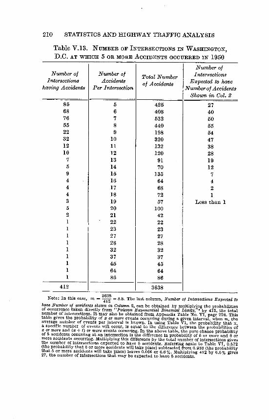
210 STATISTICS AND HIGHWAY TRAFFIC ANALYSIS
Table V.13. NumBER OF INTERSECTIONS IN WASIIINGTON,
D.C. AT wmcH 5 OR moRE ACCIDENTS OCCURRED IN 1950
Number of Number of Number of Total Number Intersections
Intersections Accidents of Accidents Expected to have
having Accidents Per Intersection Numberof Accidents
Shown in Col. 2
85 5 425 27
68 6 408 40
76 7 532 60
55 8 440 55
22 9 198 54
32 10 320 47
12 11 132 38
10 12 120 28
7 13 91 19
6 14 70 12
9 15 135 7
4 16 64 4
4 17 68 2
4 18 72 1
3 19 57 Less than 1
5 20 100
2 21 42
1 22 22
1 23 23
1 27 27
1 28 28
1 32 32
1 37 37
1 45 45
1 64 64
1 86 86
412 3638
Note: In this case, rn 3638 8.8. The last column, Number of Intersections Expected to
have Number of accidents shown in Column 2, can be obtained by multiplying the probabilities of occurrence taken directly from "Poisgon Exponential Binomial Limits,"' by 412, the total number of intersections. it may also be obtained from Appendix Table No. VI, page 226. This table gives the probability of x or more events occurring during a given interval, when m, the average number of events per interval is known. In using Table VI, the probability that x, * specific number of events will occur, is equal to the difference between tile probabilities of * or more and (x + 1) or more events occurring. In the above table, the pure chance probability of 5 accidents occurring at an intersection is the difference in probability of 5 or more and 6 or more accidents occurring. Multiplying this difference by the total number of intersections givesthe number of intersections expected to have 6 accidents. Referring again to Table VI, 0.872 (the probability that 6 or more accidents will take place) subtracted from 0.938 (the probability that 5 or more accidents will take place) leaves 0.066 or 6.6 %. Multiplying 412 by 6.6 % gives 27, the number of intersections that may be expected to have 5 accidents.

211 APPLICATIONS OF STATISTICAL METHODS
of sample to give a 95 per cent assurance that the mean valuewill
not be in error more than 0. 1. Suppose that the following typical occupancy count has been
made:
Occupants(x)
1
2
3 4
5
Number of Observations (f)
15
10
4 2
1
Mean ;.-- X = 1.9 N = 32
The standard deviation s is first calculated and found to be 1.054. From formula IV.7.3.
N- I S2 (1.054)2 1.1 I
2 2 .1)2 .01
From Appendix Table 3, Ratio of Degrees of Freedom to (t2), We
find that with a probability level of 5 per cent (95 per cent assur,92
ance) that for N - I 400, that 103.069 and for N - 1
0 500, ii = 128.836. Since II I lies between these two valueswe
conclude that the size of sample required is between 400 and 500,
and if we wish to be conservative we take the higher value. Also it would have been better to have taken a larger (preliminary)
sample to obtain the trial standard deviation.
V. 31. Size of Sample Required in Speed Study. It is desired toknow
the average speed on each block within one mile per hour on a
street with 60 intersections. It is also desired that there be a 95
per cent assurance as to the result. It is assumed that the speed
will vary with the volume of traffic, the weather, the amount of
parking, and perhaps other conditions. The problem is to find the
required size of sample and, having determined this, to recom
mend a method of making the observationsthat will yield a truly
random sample.
212 STATISTICS AND HIGHWAY TRAFFIC ANALYSIS
The logical procedure is to take a random sample of about 100 observations in order to obtain an estimated standard deviation to be used in determining the size of sample. Suppose from this sample that it is found that the speed range is from 5 to 40 miles per hour and that the standard deviation, s, equals 4.5 miles per hour.
We use the t-distributionto find the size of sample. From formula IV.7.3.
N-I S2
t2 C2
we find the ratio of N -1 to t2 by insertingthe values for s and c. The standard deviation s in the present example, as found from the preliminary sample, is 4.5 miles per hour and the allowable error is one mile per hour.
N-1- S2 (4.5)2 20.25 Hence, - - - - _= - == 20.25
t2 p2 12 1
From a table of ratio of degrees of freedom tot2we find that
with a probabilitylevel of 6 per cent that a ratio of N-I 20.202 t2
corre-onds to N 1 = 80 and 22.727 correspondsto N - 1 90. Therefore, we conclude that N, the size of sample, lies between 81 and 91. To be on the safe side, we may say that a sample of 100 observations will give us at least a 95 per cent assurance that the average speed will be obtained within ± I mile per hour. If a 99 per cent assurance is desired the size of sample according to the table would be between 100 and 200.
The next phase of the problem is that of getting a truly random sample. Obviously taking all the speeds on a day of light traffic would give a biased result. Clearly there must be some knowledge of the relative duration of the various conditions that influence speeds. Increasing the size of the sampleso that observationsmight "e distributed over a greater number of hours of the day, more days of the week and more months of the year would assure a better estimate of the speed. Increasing the size of sample to 200 should give sufficient coverage.
213 APPLICATIONS OF STATISTICAL METHODS
Since the speed is desired for each block it is necessary that
observations be taken in each block. Some accurate mechanical
device that is free from human errors is always preferable. This,
however, would require either 60 recording devices or a rotation
of a lesser number. Since they would give "spot" checks they
would also need to be rotated to different positions in the blocks.
Another way would be to have an observer's car "float" with
the traffic. The observer as well as recording speed could also note
pertinent information such as the amount of parking. Manual re
cording could be supplemented or replaced by some mechanical
device such as takinga picture of the conditionsin each block and
including in the picture a clock to show the time of reaching each intersection. The cost of such pictures taken on 16 mm film would
be negligible.
The particularmethod to be employed in this or any other problem involving the collection and analysis of data should be se
lected by the engineer in charge after he has made a preliminary
study of both the nature of the data and the reliability and cost of
the various possible methods of conducting the field study. Sta
tistics is merely an aid to the engineer and not a substitute for
experience and judgment.
RE, FERENCES, CHATTER V
"Highway Capacity Manual," Committee on Highway Capacity, De
partment of Traffic and Operation, Highway Research Board, Washington,
D.C., 1950.
2 Hess, Dr. Victor F., "The Capacity of a Highway," Traffic Engineering,
Institute of Traffic Engineers, New Haven, Connecticut, August 1950,
page 420.
3 Greenshields, Bruce D., "The Photographic Method of Studying Traffic
Behavior," Proceedings,Highway Research Board, Washington, D.C., 1933.
4 Ibid., "A Study of Traffic Capacity," Proceedings, Highway Research
Board, Washington, D.C., 1933.
5 Ibid., "Initial Traffic Interferences," Presented for discussion at the
16th Annual Meeting of the Highway Research Board, November 19, 1936,
Washington, D.C., 9 pages mimeo and the comments by W. F. Adams.
6 Ibid., "Distance and Time Required to Overtake, and Pass Cars," Pro
ceedings, Highway Research Board, Washington, D.C., 1935, pages
332-342.

214 STATISTICS AND HIGHWAY TRAFFIC ANALYSIS
7 Ibid., Schapiro, Donald; Ericksen, Elroy L. "Traffic Performance at Urban Street Intersections," Yale University, Bureau of Highway Traffic, New Haven, Connecticut, 1947.
8 "Digest of the, Application of Theory of Probability to Problems of Highway Traffic," Proceedings, Institute of Traffic Engineers, New Haven, Connecticut, 1934, pages 118-123.
9 Molina, E. C., ".Poimon Exponential Binomial Limits," (Table) D. Van Nostrand Co., New York, 1942.
10 Wynn, Houston F.; Gourlay, Stewart M.; and Strickland, Richard, I., "Study of Weaving and Merging Traffic," Technical Report No. 4, Yale University, Bureau of Highway Traffic, New Haven, Connecticut.
11 Raff, Morton S., and Hart, Jack W., "A Volume Warrant for Urban Stop Signs," Eno Foundation for Highway Traffic Control, Inc., Saugatuck, Connecticut, 1950.
12 Adams, W. F., "Road Traffic Considered as a Random Series," Journal of the Institute of Civil Engineers, London, 1936.
18 Quimby, Warren S., "Behavior Patterns for Merging Traffic," Student Thesis, Yale 'University, Bureau of Highway Traffic, New Haven, Connecticut, 1949, page 40.
14 Johnson, Dr. H. M., "Phe Detection of Accident-Prone Drivers," Proceedings, Highway Research Board, Washington, D.C., 1937, pages 444-454.
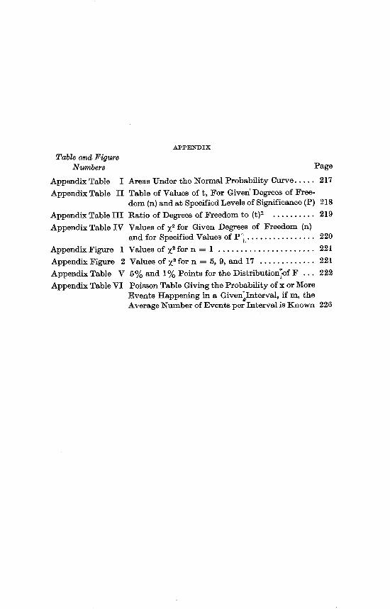
AprENDix
Table and Figure Numbem Page
Appendix Table I Areas Under the Normal Probability Curve ..... 217
Appendix Table II Table of Values of t, For GivedDegrees of Free.
Appendix Table IV Values of X2 for Given Degrees of Freedom (n)
Appendix Table VI Poisson Table Giving the Probabilityof x or MoreEvents Happening in a Given.Interval, if m, the
dom (n) and at Specified Levels of Significance (P) 218
Appendix Table III Ratio of Degrees of Freedom to (t)2 .......... 219
and for Specified Values of P'L ................ 220AppendixFigure I Values of X2 for n = 1 ...................... 221
AppendixFigure 2 Values of X2 for n = 5, 9, and 17 ............. 221
AppendixTable V 5% and I% Points for the Distribution7of F ... 222
Average Number of Events per Interval is Known 226

APPENDIX 217
APPENDIX Table I
Areas Under the Normal Probability Curve
From the Mean to Distances x from the Mean, Expressed as Decimal
Fractions of the Total Area 1.0000 The proportionalpart of the curve included between an ordinate erected
at the mean and an ordinate erected at any given value on the X axis can be read from the table by determiningx (the deviation of the given value
from the mean) and computing x Thus if $25.00, a = $4.00, and
it is desired to ascertain the proportionof the area under the curve between x $5.00ordinates erected at the mean and at $20.00; x = $5.00 and - = CT $4.00
1.25. From the table it is found that .3944, or 39.44 per cent, of theentire area is included.
X.00 01 .02 .03 .04 .05 .06 .07 .08 .09
0.0 .0000 .0040 .0080 .0120 .0159 .0199 .0239 .0279 .0319 .03590.1 .0398 .0438 .0478 .0517 .0557 .0596 .0636 .0675 .0714 .07530.2 .0793 .0832 .0871 .0910 .0948 .0987 .1026 .1064 .1103 .11410.3 .1179 .1217 .1255 .1293 .1331 .1368 .1406 .1443 .1480 .15170.4 .1564 .1591 .1628 .1664 .1700 .1736 .1772 .1808 .1844 .1879
0.5 .1916 .1950 .1985 .2019 .2054 .2088 .2123 .2157 .2190 .22240.6 .2257 .2291 .2324 .2357 .2389 .2422 .2454 .2486 .2518 .25490.7 .2580 .2612 .2642 .2673 .2704 .2734 .2764 .2794 .2823 .28620.8 .2881 .2910 .2939 .2967 .2995 .3023 .3051 .3078 .3106 .31330.9 .3159 .3186 .3212 .3238 .3264 .3289 .3315 .3340 .3365 .3389
1.0 .3413 .3438 .3461 .3485 .3508 .3531 .3554 .3577 .3599 .36211.1 .3643 .3665 .3686 .3718 .3729 .3749 .3770 .3790 .3810 .38301.2 .3849 .3869 .3888 .3907 .3925 .3944 .3962 .3980 .3997 .40151.3 .4032 .4049 .4066 .4083 .4099 .4115 .4131 .4147 .4162 .41771.4 .4192 .4207 .4222 .4236 .4251 .4265 .4279 .4292 .4306 .4319
1.5 .4332 .4345 .4357 .4370 .4382 .4394 .4406 .4418 .4430 .44411.6 .4452 .4463 .4474 .4485 .4495 .4505 .4515 .4525 .4535 .45451.7 .4554 .4564 .4573 .4582 .4591 .4599 .4608 .4616 .4625 .46331.8 .4641 .4649 .4666 .4664 .4671 .4678 .4686 .4693 .4699 .47061.9 .4713 .4719 .4726 .4732 .4738 .4744 .4750 .4758 .4762 .4767
2.0 .4773 .4778 .4783 .4788 .4793 .4798 .4803 .4808 .4812 .48172.1 .4821 .4826 .4830 .4834 .4838 .4842 .4846 .4850 .4854 .48572.2 .4861 .4865 .4868 .4871 .4875 .4878 .4881 .4884 .4887 .48902.3 .4893 .4896 .4898 .4901 .4904 .4906 .4909 .4911 .4913 .49162.4 .4918 .4920 .4922 .4925 .4927 .4929 .4931 .4932 .4934 .4936
2.5 .4938 .4940 .4941 .4943 .4945 .4946 .4948 .4949 .4951 .49522.6 .4953 .4955 .4956 .4957 .4959 .4960 .4961 .4962 .4963 .49642.7 .4965 .4966 .4967 .4968 .4969 .4970 .4971 .4972 .4973 .49742.8 .4974 .4976 .4976 .4977 .4977 .4978 .4979 .4980 .4980 .49812.9 .4981 .4982 .4983 .4984 .4984 .4984 .4985 .4985 .4986 .4986
3.0 .49865 .4987 .4987 .4988 .4988 .4988 .4989 .4989 .4989 .49903.1 .49903 .4991 .4991 .4991 .4992 .4992 .4902 .4992 .4993 .49933.2 .49931293.3 .49961663.4 .49966313.5 .4997674
3.6 .49984093.7 .49989223.8 .49992773.9 .49995194.0 .4999683
4.5 .4999966
Methode
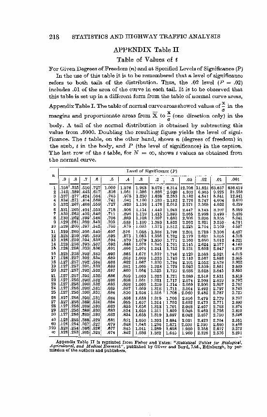
218 STATISTICS AND HIGHWAY TRAFFIC ANALYSIS
APPENDIX Table II
Table of Values of t For Given Degrees ofFreedom (n) andat Specified Levels of Significance (P)
In the use of this table it is to be remembered that a level of significance refers to both tails of the distribution. Thus, the .02 level (P = .02) includes .01 of the area of the curve in each tail. It is to be observed that this table is set up in a different form from the table of normal curve areas,
Appendix Table I. The table of normalcurve areasshowed values ofx- in the a
margins and proportionate areas from K to x- (one direction only) in the
body. A tail of the normal distribution is obtained by subtracting this value from .5000. Doubling the resulting figure yields the level of significance. The t table, on the other hand, shows n (degrees of freedom) in the stub, t in the body, and P (the level of significance) in the caption. The last row of the t table, for N = oo, shows t values as obtained from the normal curve.
Level of Significance (P)Ift
.9 .8 .7 .6 .5 .4 .3 .2 .1 .05 .02 .01 .001 1 .158 .325 .510 .727 1.000 1.376 1.963 3.078 6.314 12.706 31.821 63.657 636.6192 .142 .289 .445 .617 .816 1.061 1.386 1.886 2.920 4.303 6.965 9.925 31.5983 .137 .277 .424 .584 .765 .978 1.250 1.638 2.353 3.182 4.541 6.841 12.9414 .134 .271 .414 .569 .741 .941 1.190 1.533 2.132 2.776 3.747 4.604 8.6105 .132 .267 .408 .559 .727 .920 1.156 1.476 2.015 2.571 3.365 4.032 6.859 6 .131 .265 .404 .553 .718 .906 1.134 1.440 1.943 2.447 3.143 3.707 5.9597 .130 .263 .402 .549 .711 .896 1.119 1.415 1.895 2.365 2.998 3.499 6.4058 .130 .262 .399 .546 .706 .889 1.108 1.397 1.860 2.306 2.896 3.355 5.0419 .129 .261 .398 .543 .703 .883 1.100 1.383 1.833 2.262 2.821 3.250 4.781
lu IZU ZUU .307 .D542 IVU .611d 1.093 1.372 1.812 2.228 2.764 3.169 4.G87 11 .129 .260 .396 .540 .697 .876 1.088 1.363 1.796 2.201 2.718 3.106 4.43712 .128 .259 .395 .539 .605 .873 1.083 1.356 1.782 2.179 2.681 3.055 4.31813 .128 .259 .394 .538 .694 .870 1.079 1.350 1.771 2.160 2.650 3.012 4.22114 .128 .258 .393 .537 .692 .868 1.076 1.345 1.761 2.145 2.624 2.977 4.14015 .128 .258 .393 .536 .691 .866 1.074 1.341 1.753 2.131 2.602 2.947 4.073 16 .128 .258 .392 .535 .690 .865 1.071 1.337 1.746 2.120 2.583 2.921 4.01517 .128 .257 .392 .534 .689 .863 1.069 1.333 1.740 2.110 2.567 2.898 3.96518 .127 .257 .392 .534 .688 .862 1.067 1.330 1.734 2.101 2.552 2.878 3.92219 .127 .257 .391 .533 .688 .861 1.066 1.328 1.729 2.093 2.539 2.861 3.88320 .127 .257 .391 .533 .687 .860 1.064 1.325 1.725 2.086 2.528 2.845 3.850 21 .127 .257 .391 .532 .686 .859 1.063 1.323 1.721 2.080 2.518 2.831 3.81922 .127 .266 .390 .532 .686 .858 1.061 1.321 1.717 2.074 2.508 2.819 3.79223 .127 .256 .390 .532 .685 .858 1.060 1.319 1.714 2.069 2.600 2.807 3.76724 .127 .256 .390 .531 .685 .867 1.069 1.318 1.711 2.064 2.492 2.797 3.74525 .127 .256 .390 .531 .684 .856 1.058 1.316 1.708 2.060 2.485 2.787 3.725 26 .127 .256 .390 .531 .684 .856 1.058 1.315 1.706 2.056 2.479 2.779 3.70727 .127 .256 .389 .531 .684 .865 1.057 1.314 1.703 2.052 2.473 2.771 3.69028 .127 .256 .389 .530 .683 .855 1.056 1.313 1.701 2.048 2.467 2.763 3.67429 .127 .256 .389 .530 .683 .854 1.055 1.311 1.699 2.045 2.462 2.756 3.65930 .127 .256 .389 .530 .683 .854 1.055 1.310 1.697 2.042 2.457 2.750 3.646 40 .126 .255 .388 .529 .681 .851 1.050 1.303 1.684 2.021 2.423 2.704 3.55160 -26 .254 .387 .527 .679 .848 1.046 1.296 1671 2000 2.3.90 2.660 3.460
120 .126 .254 .386 .526 .677 .845 1.041 1.289 1:658 580 2.358 2.617 .3.373 oo .126 .253 .385 .524 .674 .842 1.282 1.645 1.960 2.326 2.576 3.291
Appendix Table 11 Is reprinted from Fisher and Yates: "Statistical Tables for Biological,Agricultural, and Medical Research", published by Oliver and Boyd, Ltd., Minburgh, by permission of the authors and publishers.

APPENDIX 219
APPENDIX
Table III
RATio OF DEGREES OF FREEDOM TO (t)2
Degrees Probability Level Of
Freedom 5% 2% 1%
1 0.006 0.001 0.0002
2 0.108 0.041 0.020
3 0.296 0.145 0.088
4 0.519 0.285 0.189
5 0.756 0.442 0.308
6 1.002 0.607 0.437
7 1.252 0.778 0.572
8 1.504 0.954 0.711
9 1.759 1.131 0.852
10 2.015 1.309 0.996
11 2.271 1.489 1.140
12 2.527 1.670 1.286
13 2.786 1.851 1.433
14 3.043 2.033 1.580
15 3.303 2.216 1.727
16 3.560 2.398 1.875
17 3.818 2.580 2.024
18 4.078 2.764 2.173
19 4.337 2.947 2.321
20 4.596 3.130 2.471
21 4.854 3.312 2.620
22 5.115 3.498 2.768
23 5.373 3.680 2.919
24 5.634 3.865 3.068
25 5.891 4.048 3.219
26 6.151 4.231 3.367
27 6.412 4.415 3.516
28 6.676 4.601 3.668
29 6.934 4.784 3.818
30 7.195 4.969 3.967
40 9.803 6.813 5.447
60 15.000 10.504 8.480
120 30.596 21.582 17.523

220 STATISTICS AND HIGHWAY TRAFFIC ANALYSIS
APPENDIX Table IV Nv_o I.DONNC =Nt_.
0 1 Oq 0! 11 1 11 1 1i 1 1 Ci 11 1 _ 11R 9 09 1 t,: 01 v: -I 'R C "! - - t: omwwo N10m N`_ ONM CMM-N ".Com
0.0 ! N N- C04 N E ONO. " N ! '" OA, I ""' ! 0"o '] I 1"i 1, ! !=' 5, Wm '!
NO,C, 0X.w Cl_10 Nmwo" NMMWN M-d-w IOlo Nw" ooom mmmm. "10wm
0 IR C! C 0! C O 1., R 11 ci t1: 0! IR _! Iq 1 ldl 1 _! 11 C 0! 14! C cl 11R 1: ai 11 -9 CO-MID 10.0 0 - M llf 0 0 0 0 M " 0 mo-N `Owmo
NNN NNNNM ,Mmmm M .... ....
N N " _Xw MNWM- M" Nmm MCo mmwoc COMMN ."m=w MN=_ mc"MN
O It - oy 11 C C 11R_! 11 1i IR C! 11 O Oi IR C 1i IR 1 O 11R C 0! 11 1 1i 11 . _O.m oww_ N=w MONM
0 1 .. - N NNNN". Nommm =mm""
H_nwo NM 1.1 M -.41 0 NN M_m MOo _Nww mm=, 00 co
0 09 c o 't, c? - R "? C IR c c 11 c 9 "? o9 1_! It e c 1i It le Ily c? L 1: =.NmId, wo Nm= HNNNN NNNmm =mmmm
N=mN mN "owo1 L`: c ci i m"m NNNN N=mmm mmmm"
N=Nc, M M O Gq NHww om"" mw_
Q N 14Rci 11 1: o! Iq o < c! It 11R oR c 1i 1 11 11 rl: c C -i 1 It Lq IR t o R -i 1! mo.Nm "Ioxm _N"c
NNNNN NNNNm mmm=.*
O.cNN m.m mmwv 4__o oWNw m_NN -cm m.O O ID M
M C 't 11Roq 1= 9 cl 1 1 L": cq R -! q cq 'R 'R t o,: CC -! o! . - , ,-N="= Damon N-111c mmoN m",Dw mo.N.
HNNN N N N N N NMMMM
M N .om mwwx ol0coo"""mm mmmw., m-mmm mmmmm o 1 1 1 1 c c? I? c ? ? c? 1 o? 1 IT I? I? 1 I? - ? 1
=mO NNN"N
wHM - - =- _- -_ : -_ H. N- . N M, :oMNNN M"Io w=N"
o! C c 1 t1: E,-: 1 1 11i i 42 N. 9m lo xmco N _ o -. 1 NN""N
-u N (D oN.*cm NN=m Lt"No omw.,
LNOm xomco oH_ Now-= C IR 1 R oq 9 1 1i c 1 11 It 1 Ili C? 1 rl 11 11 c 1_ c 11 c 117 9 It 1
mm".z= low=o lo w 00 oo.Nm NNNN
41 co m"No N_m owc,= N"=w=
o <o!9c c -q o 1 IR oR IR 1! .lz - NNmv" o=tw mooN
N N n w-o. m - Woom mcMN4 = ,N _Z;o ,'NDz,
IR o 1_! o lioR HNNmm o 1' ID k- co = o 0 N M M.* C, c M
MNd,
"""Nm =wnw "f 'D mmmo ow owm om oN"o
0 c 1 q 11 c 1 _! El: o C 11Rci c 11 oi a 11Ro! c 11 It 1i 1 9 v HNNm ml*" wwm mo-N M " c
0
N=mw moc cqcomo NIDIZ w==m oNHMo mm _o=N Q m OON c o
c _ c I? c c! 11 c? 9 C? 9 _ 11 D! "y t R 9 og L, og t ? o!,: H-NN co M 00moo- N N M
Nm" Dtmo NNNNN NNNNm
For large values of n compute 0ji, the distribution of which is ap.
proximately normal around a mean of f2n - I with a 1. P is the ratio
of one tail of the normal distribution to the area under the entire curve.
A detailed table of the probability of various values of Z' for one degree
of freedom is given in G. U. Yule and M. G. Kendall, An Introduction to the
Theory of Statistics, Ilth edition, pp. 534-535, Charles Griffin and Co.,
London,1937.
Appendix Table IV is reprinted from Fisher and Yates: "Statistical Tables for Biological, Agricultural, and Medical Research", published by Oliver and Boyd, Ltd., Edinburgh, by permission of the authors and publishers.

APPENDIX 221
APPENDIX REATIVE HEIGHT FiGURE I & II OF ORDINATE
2 3 4
RELATIVE HEIGHT VALUE OF X' OF ORDINATE
,n= 5
n. p
.X,
0 2 4 6 8 10 12 14 16 18 20 22 24 26 28 30
VALUE OF X.
Distribution of X2 for n = 1, n = 5, n = 9, and n = 17. The maximum
ordinate is at 72 = n - 2 except when n = 1. When n = 1, the max
imum ordinate is at Z2 0. When n = 1, there is 4.55 per cent of the
curve beyond X2 = 4. Beyond Z2 = 30 there is .0015 of one per cent
of the curve when n = 5; .0439 of one per cent of the curve when n = 9;
2.6345 per cent of the curve when n = 17. The two charts have been
drawn to different scales. If the vertical axis of the upper chart is ex
panded to approximately 20 times its length and the horizontal axis is
contracted to about one-eighth of its length, the curves will be roughly
comparable as to area.

5
10
15
20
25
222 STATISTICS AND HIGHWAY TRAFFIC ANALYSIS
APPEN5 0/0 and 1 0/, Points for Distribution of F,
n, degrees of freedom (for greater mean square)n,
1 2 3 4 6 6 7 8 9 10 11 12
1 1614,052
2004,999
2165,403
2265,625
2305,764
2345,859
2375,928
2395,981
2416,022
2426,056
2436,082
2446,106
2 18.51 98.49
19.00 99.00
19.16 99.17
19.25 99.25
19.30 99.30
19.33 99.33
19.36 99.34
19.37 99.36
19.38 99.38
19.39 99.40
19.40 99.41
10.41 99.42
3 10.1334.12
9.5530.82
9.2829.46
9.1228.71
9.0128.24
8.9427.91
8.8827.67
8.8427.49
8.8127.34
8.7827.23
8.7627.13
8.7427.05
4 7.7121.20
6.9418.00
6.5916.69
6.3915.98
6.2615.52
6.1615.21
6.0914.98
6.0414.80
6.0014.66
5.9614.54
5.9314.45
5.9114.37
6.6116.26
5.7913.27
5.4112.06
5.1911.39
5.0510.97
4.9510.67
4.8810.45
4.8210.27
4.7810.15
4.7410.05
4.709.96
4.689.89
6 5.0913.74
5.1410.92
4.769.78
4.539.15
4.398.75
4.288.47
4.218.26
4.158.10
4.107.98
4.067.87
4.037.79
4.007.72
7 5.5912.25
4.749.55
4.358.45
4.127.85
3.977.46
3.877.19
3.797.00
3.736.84
3.686.71
3.636.62
3.606.54
3.576.47
8 6.3211.26
4.468.65
4.077.59
3.847.01
3.696.63
3.586.37
3.506.19
3.446.03
3.395.91
3.345.82
3.315.74
3.295.67
9 5.1210.56
4.268.02
3.866.99
3.636.42
3.486.06
3.375.80
3.295.62
3.235.47
3.185.35
3.135.26
3.105.18
3.075.11
4.9610.04
4.107.56
3.716.55
3.485.99
3.335.64
3.225.39
3.145.21
3.075.06
3.024.95
2.974.85
2.944.78
2.914.71
11 4.849.65
3.987.20
3.596.22
3.365.67
3.205.32
3.095.07
3.014.88
2.954.74
2.904.63
2.864.54
2.824.46
2.794.40
12 4.759.33
3.886.93
3.495.95
3.265.41
3.115.06
3.004.82
2.924.65
2.854.50
2.804.39
2.764.30
2.724.22
2.694.16
is 4.679.07
3.806.70
3.415.74
3.185.20
3.024.86
2.924.62
2.844.44
2.774.30
2.724.19
2.674.10
2.634.02
2.603.96
14 4.608.86
3.746.51
3.345.56
3.115.03
2.964.69
2.854.46
2.774.28
2.704.14
2.654.03
2.603.94
2.563.86
2.533.80
4.548.68
3.686.36
3.295.42
3.064.89
2.904.56
2.794.32
2.704.14
2.644.00
2.593.89
2.553.80
2.513.73
2.493.67
16 4.498.53
3.636.23
3.245.29
3.014.77
2.854.44
2.744.20
2.664.03
2.593.89
2.543.78
2.493.69
2.453.61
2.423.55
17 4.458.40
3.596.11
3.205.18
2.964.67
2.814.34
2.704.10
2.623.93
2.553.79
2.503.68
2.453.59
2.413.52
2.383.45
18 4.418.28
3.556.01
3.165.09
2.934.58
2.774.25
2.664.01
2.583.85
2.513.71
2.463.60
2.413.51
2.373.44
2.343.37
19 4.388.18
3.525.93
3.135.01
2.904.50
2.744.17
2.633.94
2.553.77
2.483.63
2.433.52
2.383.43
2.343.36
2.313.30
4.358.10
3.495.85
3.104.94
2.874.43
2.714.10
2.603.87
2.523.71
2.453.56
2.403.46
2.353.37
2.313.30
2.283.23
21 4.328.02
3.475.78
3.074.87
2.844.37
2.684.04
2.573.81
2.493.65
2.423.51
2.373.40
2.323.31
2.283.24
2.253.17
22 4.307.94
3.445.72
3.054.82
2.824.31
2.663.99
2.553.76
2.473.59
2.403.45
2.353.35
2.303.26
2.263.18
2.233.12
23 4.287.88
3.425.66
3.034.76
2.804.26
2.643.94
2.533.71
2.453.54
2.383.41
2.323.30
2.283.21
2.243.14
2.203.07
24 4.267.82
3.405.61
3.014.72
2.784.22
2.623.90
2.513.67
2.433.50
2.363.36
2.303.25
2.263.17
2.223.09
2.183.03
4.247.77
3.385.57
2.994.68
2.764.18
2.603.86
2.493.63
2.413.46
2.343.32
2.283.21
2.243.13
2.203.05
2.162.99
26 4.227.72
3.375.53
2.984.64
2.744.14
2.593.82
2.473.59
2.393.42
2.323.29
2.273.17
2.223.09
2.183.02
2.152.96
The function, F= e with exponent 2z, is computed in part from Fisher's table VI (7). Ad-Used by Permission of Iowa State College Press, Publishers of Snedecor's
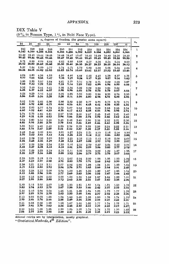
APPENDIX 223
DIX Table V(5 0/, in Roman Type, I 0/( in Bold Face Type).
n, degrees of freedom (for greater mean square)14 16 20 24 30 40 50 75 100 200 500 00
245 246 248 249 250 251 252 253 253 254 254 254 16,142 6,169 6,208 6,234 6,258 6,286 6,302 6,323 6.334 6,352 6,361 6,366 19.42 19.43 19.44 19.45 19.46 19.47 19.47 19.48 10.49 19.49 19.50 19.50 299.43 99.44 99.45 99.46 99.47 99.48 99.48 99.49 99.49 99.49 99.50 99.50
8.71 8.69 8.66 8.64 8.62 8.60 8.58 8.57 8.56 8.54 8.54 8.53 326.92 26.83 26.69 26.60 26.50 26.41 26.35 26.27 26.23 26.18 26.14 26.12 5.87 5.84 5.80 5.77 5.74 5.71 5.70 5.68 6.66 5.65 5.64 5.63 4
14.24 14.15 14.02 13.93 13.83 13.74 13.69 13.61 13.57 13.52 13.48 13.46
4.64 4.60 4.56 4.53 4.50 4.46 4.44 4.42 4.40 4.38 4.37 4.36 59.77 9.68 9.55 9.47 9.38 9.29 9.74 9.17 9.13 9.07 9.04 9.02 3.96 3.92 3.87 3.84 3.81 3.77 3.75 3.72 3.71 3.69 3.68 3.67 67.60 7.52 7.39 7.31 7.23 7.14 7.09 7.02 6.99 6.94 6.90 6.88 3.62 3.49 3.44 3.41 3.38 3.34 3.32 3.29 8.28 3.25 3.24 76.35 6.27 6.15 6.07 5.98 5.90 5.85 5.78 5.75 5.70 5.67 5.65 3.23 3.20 3.15 3.12 3.08 3.05 3.03 3.00 2.98 2.96 2.94 2.93 85.56 5.48 5.36 5.28 5.20 5.11 5.06 5.00 4.96 4.91 4.88 4.86
3.02 2.98 2.93 2.90 2.86 2.82 2.80 2.77 2.76 2.73 2.72 2.71 95.00 4.92 4.80 4.73 4.64 4.56 4.51 4.45 4.41 4.36 4.33 4.31 2.86 2.82 2.77 2.74 2.70 2.67 2.64 2.61 2.59 2.56 2.55 2.64 104.60 4.52 4.41 4.33 4.25 4.17 4.12 4.05 4.01 3.96 3.93 3.91 2.74 2.70 2.65 2.61 2.57 2.53 2.50 2.47 2.45 2.42 2.41 2.40 114.29 4.21 4.10 4.02 3.94 3.86 3.80 3.74 3.70 3.66 3.62 3.60 2.64 2.60 2.54 2.50 2.46 2.42 2.40 2.36 2.35 2.32 2.31 2.30 124.05 3.98 3.86 3.78 3.70 3.61 3.56 3.49 3.46 3.41 3.38 3.36 2.55 2.51 2.46 2.42 2.38 2.34 2.32 2.28 2.26 2.24 2.22 2.21 133.85 3.78 3.67 3.59 3.51 3.42 3.37 3.30 3.27 3.21 3.18 3.16 2.48 2.44 2.39 2.35 2.31 2.27 2.24 2.21 2.19 2.16 2.14 2.13 143.70 3.62 3.51 3.43 3.34 3.26 3.21 3.14 3.11 3.06 3.02 3.00 2.43 2.39 2.33 2.29 2.25 2.21 2.18 2.15 2.12 2.10 2.08 2.07 153.56 3.48 3.36 3.29 3.20 3.12 3.07 3.00 2.97 2.92 2.89 2.87 2.37 2.33 2.28 2.24 2.20 2.16 2.13 2.09 2.07 2.04 2.02 2.01 163.45 3.37 3.25 3.18 3.10 3.01 2.96 2.89 2.86 2.80 2.77 2.75 2.33 2.29 2.23 2.19 2.15 2.11 2.08 2.04 2.02 1.99 1.97 1.96 173.35 3.27 3.16 3.08 3.00 2.92 2.86 2.79 2.76 2.70 2.67 2.65
2.29 2.25 2.19 2.15 2.11 2.07 2.04 2.00 1.98 1.95 1.93 1.92 183.27 3.19 3.07 3.00 2.91 2.83 2.78 2.71 2.68 2.62 2.59 2.57 2.26 2.21 2.15 2.11 2.07 2.02 2.00 1.96 1.94 1.91 1.90 1.88 193.19 3.12 3.00 2.92 2.84 2.76 2.70 2.63 2.60 2.54 2.51 2.49 2.23 2.18 2.12 2.08 2.04 1.99 1.96 1.92 1.90 1.87 1.85 1.84 203.13 3.05 2.94 2.86 2.77 2.69 2.63 2.56 2.53 2.47 2.44 2.42 2.20 2.15 2.09 2.05 2.00 1.96 1.93 1.89 1.87 1.84 1.82 1.81 213.07 2.99 2.88 2.80 2.72 2.63 2.58 2.51 2.47 2.42 2.38 2.36
2.18 2.13 2.07 2.03 1.08 1.93 1.91 1.87 1.84 1.81 1.80 1.78 223.02 2.94 2.83 2.75 2.67 2.58 2.53 2.46 2.42 2.37 2.33 2.31 2.14 2.10 2.04 2.00 1.96 1.91 1.88 1.84 1.82 1.79 1.77 1.76 232.97 2.89 2.78 2.70 2.62 2.53 2.48 2.41 2.37 2.32 2.28 2.26 2.13 2.09 2.02 1,98 1.94 1.89 1.86 1.82 1.80 1.76 1.74 1.73 242.93 2.85 2.74 2.66 2.58 2.49 2.44 2.36 2.33 2.27 2.23 2.21 2.11 2.06 2.00 1,96 1.92 1.87 1.84 1.80 1.77 1.74 1.72 1.71 252.89 2.81 2.70 2.62 2.54 2.45 2.40 2.32 2.29 2.23 2.19 2.17 2.10 2.05- 1.09 1,05 1.90 1.85 1.82 1.78 1.76 1.72 1.70 1 691 262.86 2.77 2.66 2,58 2.50 2.41 2.36 2.28 2.25 2.19 2.15 2:13
ditional entries are by interpolation, mostly graphical. -StatisticalMethodsl4th Edition".

224 STATISTICS AND HIGHWAY TRAFFIC ANALYSIS
APPENDIX
50/, and I 0/, Points for the Distribution of F.
degrees of freedom (for greater mean square)
1 2 3 4 6 6 7 8 9 10 11 12
27 4.21 3.35 2.96 2.73 2.57 2.46 2.37 2.30 2.25 2.20 2.16 2.13 7.68 5.49 4.60 4.11 3.79 3.56 3.39 3.26 3.14 3.06 2.98 2.93
28 4.20 3.34 2.95 2.71 2.56 2.44 2.36 2.29 2.24 2.19 2.15 2.12 7.64 5.45 4.57 4.07 3.76 3.53 3.36 3.23 3.11 3.03 2.95 2.90
29 4.18 3.33 2.93 2.70 2.54 2.43 2.35 2.28 2.22 2.18 2.14 2.10 7.60 5.42 4.54 4.04 3.73 3.50 3.33 3.20 3.08 3.00 2.92 2.87
30 4.17 3.32 2.92 2.69 2.53 2.42 2.34 2.27 2.21 2.16 2.12 2.09 7.56 5.39 4.51 4.02 3.70 3.47 3.30 3.17 3.06 2.98 2.90 2.84
32 4.15 3.30 2.90 2.67 2.51 2.40 2.32 2.25 2.19 2.14 2.10 2.07 7.50 5.34 4.46 3.97 3.66 3.42 3.25 3.12 3.01 2.94 2.86 2.80
34 4.13 3.28 2.88 2.66 2.49 2.38 2.30 2.23 2.17 2.12 2.08 2.05 7.44 5.29 4.42 3.93 3.61 3.38 3.21 3.08 2.97 2.89 2.82 2.76
36 4.11 3.26 2.86 2.63 2.48 2.36 2.28 2.21 2.15 2.10 2.06 2.03 7.39 5.25 4.38 3.89 3.58 3.35 3.18 3.04 2.94 2.86 2.78 2.72
38 4.10 3.25 2.85 2.62 2.46 2.35 2.26 2.19 2.14 2.09 2.05 2.02 7.35 5.21 4.34 3.86 3.54 3.32 3.15 3.02 2.91 2.82 2,75 2.69
40 4.08 3.23 2.84 2.61 2.45 2.34 2.25 2.18 2.12 2.07 2.04 2.00 7.31 5.18 4.31 3.83 3.51 3.29 3.12 2.99 2.88 2.80 2.73 2.66
42 4.07 3.22 2.83 2.59 2.44 2.32 2.24 2.17 2.11 2.06 2.02 1.99 7.27 5.15 4.29 3.80 3.49 3.26 3.10 2.96 2.86 2.77 2.70 2.64
44 4.06 3.21 2.82 2.58 2.43 2.31 2.23 2.16 2.10 2.05 2.01 1.98 7.24 5.12 4.26 3.78 3.46 3.24 3.07 2.94 2.84 2.75 2.68 2.62
46 4.05 3.20 2.81 2.57 2.42 2.30 2.22 2.14 2.09 2.04 2.00 1.97 7.21 5.10 4.24 3.76 3.44 3.22 3.05 2.92 2.82 2.73 2.66 2.60
48 4.04 3.19 2.80 2.56 2.41 2.30 2.21 2.14 2.08 2.03 1.00 1.06 7.19 5.08 4.22 3.74 3.42 3.20 3.04 2.90 2.80 2.71 2.64 2.58
50 4.03 3.18 2.79 2.56 2.40 2.29 2.20 2.13 2.07 2.02 1.98 1.95 7.17 5.06 4.20 3.72 3.41 3.18 3.02 2.88 2.78 2.70 2.62 2.56
55 4.02 7.12
3.] 7 5.01
2.78 2.54 2.38 2.27 2.18 2.11 2.05 2.00 1.97 1.93 4.16 3.68 3.37 3.15 2.98 2.85 2.75 2.66 2.59 2.53
60 4.00 3.15 2.76 2.52 2.37 2.25 2.17 2.10 2.04 1.99 1.95 1.92 7.08 4.98 4.13 3.65 3.34 3.12 2.95 2.82 2.72 2.63 2.56 2.50
65 3.99 3.14 2.75 2.51 2.36 2.24 2.15 2.08 2.02 1.98 1.94 1.90 7.04 4.95 4.10 3.62 3.31 3.09 2.93 2.79 2.70 2.61 2.54 2.47
70 3.98 3.13 2.74 2.50 2.35 2.23 2.14 2.07 2.01 1.97 1.93 1.89 7.01 4.92 4.08 3.60 3.29 3.07 2.91 2.77 2.67 2.59 2.51 2.45
80 3.96 3.11 2.72 2.48 2.33 2.21 2.12 2.05 1.99 1.95 1.91 1.88 6.96 4.88 4.04 3.56 3.25 3.04 2.87 2.74 2.64 2.55 2.48 2.41
100 3.04 3.09 2.70 2.46 2.30 2.10 2.10 2.03 1.97 1.92 1.88 1.85 6.90 4.82 3.98 3.51 3.20 2.99 2.82 2.69 2.59 2.51 2.43 2.36
125 3.92 3.07 2.68 2.44 2.29 2.17 2.08 2.01 1.05 1.90 1.86 1.83 6.84 4.78 3.94 3.47 3.17 2.95 2.79 2.65 2.56 2.47 2.40 2.33
150 3.91 3.06 2.67 2.43 2.27 2.16 2.07 2.00 1.94 1.89 1.85 1.82 6.81 4.75 3.91 3.44 3.14 2.92 2.76 2.62 2.53 2." 2.37 2.30
200 3.89 3.04 2.65 2.41 2.26 2.14 2.05 1.98 1.92 1.87 1.83 1.80 6.76 4.71 3.88 3.41 3.11 2.90 2.73 2.60 2.50 2.41 2.34 2.28
400 3.86 3.02 2.62 2.39 2.23 2.12 2.03 1.96 1.90 1.85 1.81 1.78 6.70 4.66 3.83 3.36 3.06 2.85 2.69 2.55 2.46 2.37 2.29 2.23
1000 3.85 3.00 2.61 2.38 2.22 2.10 2.02 1.95 1.89 1.84 1.80 1.76 6.66 4.62 3.80 3.34 3.04 2.82 2.66 2.53 2.43 2.34 2.26 2.20
00 3.84 2.99 2.60 2.37 2.21 2.09 2.01 1.94 1.88 1.83 1.79 1.75 6.64 4.60 3.78 3.32 3.02 2.80 2.64 2.51 2.41 2.32 2.24 2.18
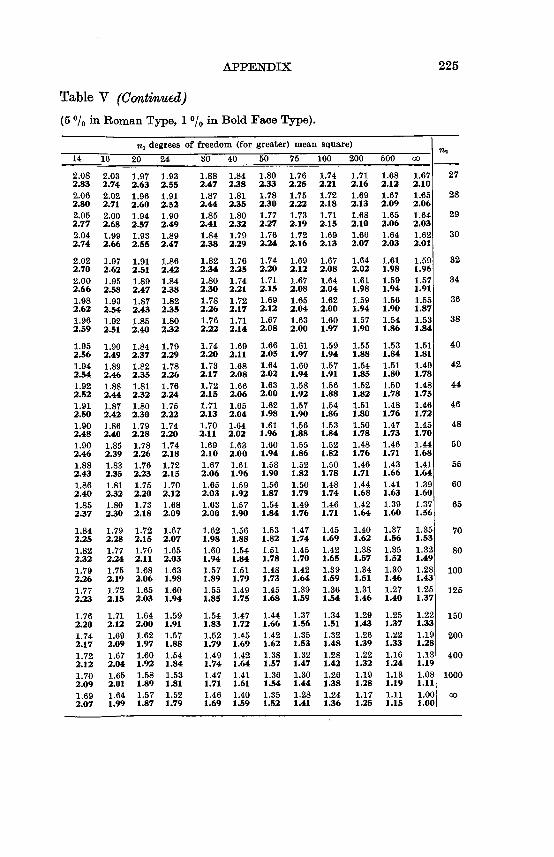
APPENDIX 225
Table V (Continued)
(5 0/, in Roman Type, 1 0/, in Bold Face Type).
n, degrees of freedom (for greater) mean square) n. 0 00
2 082:83
2032:74
1 972:63
1.932.55
1.882.47
1.842.38
1.802.33
1.762.25
1.742.21
1.712.16
1.682.12
1.672.10
27
2.062.80
2.022.71
1.962.60
1.912.52
1.872.44
1.812.35
1.782.30
1.752.22
1.722.18
1.692.13
1.672.09
1.652.06
28
2.052.77
2.002.68
1.942.57
1.902.49
1.852.41
1.802.32
1.772.27
1.732.19
1.712.15
1.682.10
1.652.06
1.642.03
29
2.042.74
1.992.66
1.932.55
1.892.47
1.842.38
1.792.29
1.762.24
1.722.16
1.692.13
1.662.07
1.642.03
1.622.01
30
2.022.70
1.972.62
1.912.51
1.862.42
1.822.34
1.762.25
1.742.20
1.692.12
1.672.08
1.642.02
1.611.98
1.591.96
32
2.002.66
1.952.58
1.892.47
1.842.38
1.802.30
1.742.21
1.712.15
1.672.08
1.642.04
1.611.98
1.691.94
1.571.91
34
1.982.62
1.932.54
1.872.43
1.822.35
1.782.26
1.722.17
1.692.12
1.652.04
1.622.00
1.591.94
1.561.90
1.551.87
36
1.962.59
1.022.51
1.852.40
1.802.32
1.762.22
1.712.14
1.672.08
1.632.00
1.601.97
1.571.90
1.541.86
1.531.84
38
1.952.56
1.902.49
1.842.37
1.792.29
1.742.20
1.692.11
1.662.05
1.611.97
1.591.94
1.551.88
L531.84
1.511.81
40
1.942.54
1.892.46
1.822.35
1.782.26
1.732.17
1.682.08
1.642.02
1.601.94
1.571.91
1.541.85
1.511.80
1.491.78
42
1.922.52
1.882."
1.812.32
1.762.24
1.722.15
1.662.06
1.632.00
1.581.92
1.561.88
1.621.82
L501.78
1.481.75
44
1.912.50
1.872.42
1.802.30
1.762.22
1.712.13
1.652.04
1.621.98
1.571.90
1.541.86
1.511.80
1.481.76
1.461.72
46
1.902.48
1.862.40
1.702.28
1.742.20
1.702.11
1.642.02
1.611.96
1.561.88
1.531.84
1.501.78
L471.73
1.451.70
48
1.902.46
1.852.39
1.782.26
1.742.18
1.692.10
1.632.00
1.601.94
1.551.86
1.521.82
1.481.76
1.461.71
1.441.68
50
1.882.43
1.832.35
1.762.23
1.722.15
1.672.06
1.611.96
1.681.90
1.521.82
1.501.78
1.461.71
1.431.66
1.411.64
55
1.862.40
1.812.32
1.752.20
1.702.12
1.652.03
1.591.92
1.561.87
1.501.79
1.481.74
1.441.68
1.411.63
1.391.60
60
1.852.37
1.802.30
1.732.18
1.682.09
1.632.00
1.571.90
1.541.84
1.491.76
1.461.71
1.421.64
1.391.60
1.371.56
65
1.842.25
1.792.28
1.722.15
1.672.07
1.621.98
1.561.88
1.531.82
1.471.74
1.451.69
1.401.62
1.371.56
1.351.53
70
1.822.32
1.772.24
1.702.11
1.652.03
1.601.94
1.541.84
1.511.78
1.451.70
1.421.65
1.381.57
1.351.52
1.321.49
80
1.792.26
1.752.19
1.682.06
1.631.98
1.571.89
1.511.79
1.481.73
1.421.64
1.391.59
1.341.51
1.301.46
1.281.43
100
1.772.23
1.722.15
1.652.03
1.601.94
1.551.85
1.491.75
1.451.68
1.391.59
1.361.54
1.311.46
1.271.40
1.251.37
125
1.762.20
1.712.12
1.642.00
1.591.91
1.541.83
1.471.72
1.441.66
1.371.56
1.341.51
1.291.43
1.251.37
1.221.33
150
1.742.17
1.692.09
1.621.97
1.571.88
1.521.79
1.451.69
1.421.62
1.351.53
1.321.48
1.261.39
1.221.33
1.191.28
200
1.722.12
1.672.04
1.601.92
1.541.84
1.491.74
1.421.64
1.381.57
1.321.47
1.281.42
1.221.32
1.161.24
1'131.19
400
1.70 1.65 1.58 1.53 1.47 1.41 1.36 1.30 1.26 1.19 1.13 1.08 1000 2.09 2.01 1.89 1.81 1.71 1.61 1.54 I." 1.38 1.28 1.19 1.11 1.60 2.07
1.64 1.99
1.57 1.87
1.52 1.79
1.46 1.69
1.40 1.59
1.35 1.52
1.28 1.41
1.24 1.36
1.17 1.25
1.11 1.15
1.00 1.00
oo

226 STATISTICS AND HIGHWAY TRAFFIC ANALYSIS
APPENDIX Table VIPOISSON TABLES
Construction of the Table Giving the Probability of x or More Events Happening in a Given Interval if W, the Average Number of Events per Interval is Known - The probability that 'x' Events will Happen in a given time or space segment is equal to
Pn e-m (MX) x
where x refers to any value of V. The value of this expression for various values of 'm' and Y is
readily available in standard Poisson tables. Thus P. may be found for any given values of 'x' and 'm'. For
example, if m = 4 and x r-- 0. e-- (mx) e-4 (40)
PO = = 0.018x! 0! If m;= 4 and x;--= I
e-M (mx) e-4 (41) 0.0183 (4)P, 0.073
x! If m = 4 and x;== 2
e-4 (42) .0183 (16) P2 = 0.1472! 2
If ln4andx=3 e-4 (43) 0.0183 (64)
P3 0.1953! 6 This procedure can of course, be continued. The probability of getting three or less is the sum of the prob
ability of getting 0, 1, 2 or 3 and therefore is equal 0.018 + 0.073 + 0.147 + 0.195 0.433 = 43.3 in 100 or 43.3 per cent. The probability of getting four or more is 56.7 out of 100 or 56.7 per cent. This followsfrom the fact that the total probability of getting all possible numbers is one or 100 per cent. This is the procedure followed in the calculation of the tables. Therefore, the values given in the tables are
0 Ml M2 M(X-1) 1 -e-m + - + - + +
(7l I ! 2 1 (x - 1)!
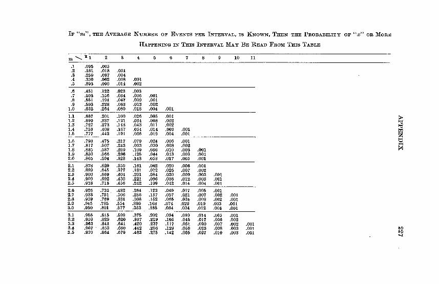
IF "m", THE AVERAGE NUMBER or EVENTS PER INTERVAL, 118 KNowN, THEN THE PROBABILITY OF "X" OR MORE
HAPPENING IN THIS INTERVAL MAY BE READ Fnom THIS TABLE
in x 1 2 3 4 5 6 7 8 9 10 11
.1 .095 .005 .2 .181 .018 .001 .3 .259 .037 .004 .4 .330 .062 .008 .001 .5 .393 .090 .014 .002
.6 .451 .122 .023 .003
.7 .603 .156 .034 .006 .001
.8 .551 .191 .047 .009 .001
.9 .593 .228 .063 .013 .002 1.0 .632 .264 .080 .018 .004 .001
1.1 .667 .301 .100 .026 .005 .001 1.2 .690 .337 .121 .034 .008 .002 1.3 .727 .373 .143 .043 .011 .002 1.4 .753 .408 .167 .054 .014 .003 .001 1.5 .777 .442 .191 .066 .019 .004 .001
1.6 .798 .475 .217 .079 .024 .006 .001 1.7 .817 .507 .243 .093 .030 .008 .002 1.8 .835 .637 .269 .109 .036 .010 .003 .001 1.9 .850 .566 .296 .125 .044 .013 .003 .001 2.0 .865 .594 .323 .143 .053 .017 .005 .001
2.1 .878 .620 .350 .161 .062 .020 .006 .001 2.2 .889 .645 .377 .181 .072 .025 .007 .002 2.3 .900 .669 .404 .201 .084 .030 .009 .003 .001 2.4 .909 .692 .430 .221 .096 .036 .012 .003 .001 2.5 .918 .713 .456 .242 .109 .042 .014 .004 .001
2.6 .926 .733 .482 .264 .123 .049 .017 .005 .001 2.7 .933 .751 .506 .286 .137 .057 .021 .007 .002 .001 2.8 .939 .769 .531 .308 .152 .065 .024 .008 .002 .001 2.9 .945 .785 .554 .330 .168 .074 .029 .010 .003 .001 3.0 .950 .801 .577 .353 .185 .084 .034 .012 .004 .001
3.1 .055 .815 .599 .375 .202 .004 .039 .014 .005 .001 3.2 .959 .829 .620 .307 .219 .105 .045 .017 .000 .002 3.3 .063 .841 .641 .420 .237 .117 .051 .020 .007 .002 .001 3.4 .967 , .853 .660 .442 .256 .129 .068 .023 .008 .003 .001 t* 3.5 .970 .864 .679 .463 .275 .142 .065 .027 .010 .003 .001

IF "M", THE AVERAcfE NumBER OF EvEirrs PER INTERVAL, is KiqowN, THEN THE PROBABILITY OF "X" OR MORE k-0
HA-Ppm-m-TG iN THis INTERVAL MAY BE READ Pitom THis TABLE 00
m X 1 2 3 4 6 6 7 8 9 10 11 12 13 14 15 16 17
3.6 3.7 3.8 3.9 4.0
.973
.075
.978
.980
.982
.874
.884
.893
.001
.908
.697
.715
.731
.747
.762
.485
.506
.527
.647
.567
.294
.313
.332
.352
.371
.156
.170
.184
.199
.215
.073
.082
.091
.101
.111
.(31
.035
.040
.045
.051
.012
.014
.016
.019
.021
.004
.005
.006
.007
.008
.001
.002
.002
.002
.003
.001 .001 .001
4.1 4.2 4.3 4.4 4.5
.983
.985 .986 .988 .989
.015
.922
.928
.934
.939
.776
.790
.803
.815
.826
.686
.605
.623
.641
.658
.391
.410
.430
.449
.468
.231
.247
.263
.280
.297
.121
.133
.144
.166
.169
.057
.064
.071
.079
.087
.024
.028
.032
.036
.040
.010
.011
.013
.015
.017
.003
.004
.005
.006
.007
.001
.001
.002
.002
.002
.001
.001
.001
4.6 4.7 4.8 4.0 5.0
.000 .991 .992 .903 .993
.044
.948 .952 .056 .960
.837 .848 .857 .867 .875
.674 .690 .706 .721 .735
.487
.605
.624
.542
.560
.314
.332
.349
.366
.384
.182
.105
.209
.233
.238
.(95
.104
.113
.123
.133
.045
.050
.056
.062
.068
.020
.022
.025
.028
.032
.008
.009
.010
.012
.014
.003
.003
.004
.005
.005
.001 .001 .001 .002 .002
.001
.001
6.1 5.2 5.3 6.4 6.6
.994
.994
.995
.995
.996
.963
.966
.969
.971
.973
.884
.891 .898 .905 .912
.749
.762
.776
.787
.798
.677 .694 .610 .627 .642
-402 .419 .437 .454 .471
.253 .268 .283 .298 .314
.144
.155
.167
.178
.191
.075 .082 .089 .097 .106
.036
.040
.044
.049 .054
.016
.018
.020
.023
.025
.006
.007
.008
.010
.011
.002
.003
.003
.004
.004
.001
.001
.001
.001
.002 .001
5.6 6.7 6.8 5.9 6.0
.996
.997
.997
.997
.998
.976
.078
.979
.981
.983
.918
.023
.928
.933
.938
.809
.820
.830
.840
.849
.658
.673
.687
.701 .715
.488
.505 .522 .538 .554
.330 .346 .362 .378 .394
.203
.216
.229
.242
.256
.114
.123
.133
.143
.153
.059
.065
.071
.077
.084
.028
.031
.035
.039
.043
.012
.014
.016 1018 .020
.005
.006 .007 .008 .009
.002
.002
.003
.003
.004
.001
.001
.001
.001
.001 .00:1 0
6.1 6.2 6.3 6.4 6.6
.998
.998
.998
.998
.998
.984
.985
.987 .988 .089
.942
.946
.950
.954
.057
.857
.866
.874 .881 .888
.728
.741
.753
.765 .776
.570
.686
.601
.616
.631 --
.410
.426 A42 .458 .473-
.270
.284
.298
.1313
.327
.163
.174
.185
.197
.208
.091
.098
.106
.114
.123
.047
.051
.056
.061
.067
.022
.025
.028
.031
.034
.010 .011 .013 .014 .016
.004
.005
.005
.006
.007
.002
.002
.002
.003
.003
.001
.001 .00:1 .001 .00:1 w
6.6 6.7 6.8 6.9 7.0
.099
.999
.999
.999
.090
.990
.991
.991
.992
.903
.060
.963
.966
.968
.970
.895
.901
.907
.913
.018
.787
.798
.808
.818
.827
.645
.659
.673
.686
.699
.489 .505 .520 .535 .550
.342
.357
.372
.386
.401
.220
.233
.245
.258
.271
.131
.140
.150
.160
.170
.073
.079
.085
.092
.099
.037
.041
.046
.049
.053
.018
.020
.022
.024 .027
.008
.009
.010
.011
.013
.003
.004
.004
.005
.006
.001
.002
.002
.002
.002
.001
.001
.001
.001
.001
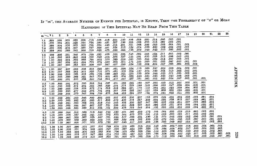
IF "M", THE AVERAGE NUMBER OF EVENTS PER INTERVAL, IS KcNowx, THEN THE PROBABILITY OF "X" Olt MORE
HAPPENING IN THIS INTERVAL MAY BE READ FROM THIS TA13LE
M X 1 --- 2 3 4 6 6 7 8 9 10 11 12 13 14 15 16 17 18 19 20 21 22 23
7.1 .099 7.2 .999 7.3 .999 7.4 .999 7.5 .999
.093 .994 .994 .995 .995
.973 .975 .976 .978 .980
.923 .928 .933 .937 .941
.830
.844
.853
.860
.868
.712
.724
.736
.747
.759
.565
.580
.594
.608
.622
.416
.431
.446
.461
.475
.284
.297
.311
.324
.338
.180
.190
.201
.212
.224
.106 .113 .121 .129 .138
.058
.063
.068
.074
.079
.030
.033
.036
.039
.043
.014 .016 .018 .020 .022
.006
.007
.008
.009
.010
.003
.003
.004
.004
.005
.001 .001 .001 .002 .002
.001
.001
.001 7.6 .999 7.7 1.00 7.8 1.00 7.9 1.00 8.0 1.00
.996
.996
.996
.997
.907
.981 .983 .984 .985 .986
.946 .948 .952 .955 .958
.875
.882
.888
.894
.900
.769
.780
.790
.799
.809
.635
.649
.662
.674
.687
.490
.504
.519
.533
.547
.352
.366
.380
.393
.407
.235
.247
.259
.271
.283
.146
.155
.165 .174 .184
.085
.091
.098 .105 .112
.046
.050 .055 .059 .064
.024
.026
.029
.031
.034
.011
.013
.014 .016 .017
.005
.006
.007
.007
.008
.002
.003 .003 .003 .004
.001
.001
.001
.001
.002 .001 .001
8.1 1.00 8.2 1.00 8.3 1.00 8.4 1.00 8.5 1.00
.997 .997 .998 .998 .998
.987 .988 .989 .990 .991
.960
.963
.965
.968
.970
.906
.911 .916 .921 .926
.818
.826 .835 .843 .850
.699
.710 .722 .733 .744
.561
.575
.588
.601
.614
.421
.435
.449
.463
.477
.296 .194
.308 .204
.321 .215
.334 .226
..347 .237
.119
.127
.135
.143
.151
.069
.074
.079
.085
.091
.037 .040 .044 .048 .051
.019
.021
.023
.025
.027
.009
.010
.011
.013
.014
.004
.005
.005 .006 .007
.002
.002
.002 .003 .003
.001
.001
.001
.001
.001 .001
0
8.6 1.00 8.7 1.00 8.8 1.00 8.9 1.00 9.0 1.00
.998
.998
.999
.999
.999
.991
.992
.993
.993
.994
.972
.974
.976
.977
.979
.930
.934
.938 .942 .945
.858 .865 .872 .878 .884
.754 .765 .774 .784 .793
.627
.640
.652 .664 .676
.491
.504
.518 .531 .544
.360
.373
.386 .399 .413
.248
.259
.271
.282
.294
.160
.169
.178
.187
.197
.097
.103
.110
.117
.124
.055
.060
.064
.069
.074
.030
.033
.035
.038
.041
.015
.017
.018
.020
.022
.007
.008
.009
.010
.011
.003
.004
.004
.005
.005
.001
.002
.002
.002
.002
.001
.001
.001
.001
.001
9.1 1.00 9.2 1.00 9.3 1.00 9.4 1.00 9.5 1.00
.999
.999
.999
.999
.999
.994
.995
.995
.995
.996
.980
.982
.983
.984
.985
.948
.951
.954
.957
.960
.890 .896 .901 .907 .911
.802 .811 .819 .827 .835
.688
.699
.710
.721
.731
.557
.570 .583 .596 .608
.426 .439 .452 .465 .478
.306
.318
.330
.342
.355
.207
.217
.227
.237
.248
.132
.139
.147
.155
.164
.079
.084
.090
.096
.102
.045
.085
.052
.056
.060
.024
.026
.028
.031
.033
.012
.013
.015
.016
.018
.006
.007
.007
.008
.009
.003
.003
.003
.004
.004
.001
.001
.002
.002
.002
.001 .001 .001 .001 .001
9.6 1.00 9.7 1.00 9.8 1.00 9.9 1.00
10.0 1.00
.999
.999
.999
.999 1.00
.996
.996
.997
.997
.997
.986
.987
.988
.989
.990
.962
.966
.967
.069
.971
.916
.921
.925
.929
.933
.843
.850
.857
.863
.870
.742
.752
.761
.771
.780
.620
.632
.644
.656
.667
.491
.604
.517
.529
.642
.367 .379 .392 .404 .417
.259
.270 .281 .202 .303
.172
.181 .190 .199 .208
.108 .115 .121 .128 .136
.064
.069
.073
.078
.083
.036
.039
.042
.045
.049
.019
.021 .023 .025 .027
.010
.011
.012
.013
.014
.005
.005
.006
.007
.007
.002
.002
.003
.003
.003
.001
.001 .001 .001 .002
.001 .001 .001
10.1 10.2 10.3 10.4 3.0.6
1.00 1.00 1.00 1.00 1.00
1.00 1.00 1.00 1.00 1.00
.997
.998
.998 .998 .998
.990
.991
.992
.092
.993
.973
.974
.976
.977
.979
.937
.940
.943
.947 .950
.876
.882
.888
.893
.898
.789
.797
.806
.814
.821
.678
.689
.700
.710
.721
.555
.567
.579
.591
.603
.429
.442
.454
.467
.479
.316
.326
.338
.350
.361
.218
.228
.238 248 .258
.143
.151
.158
.166
.175
.089
.094
.100
.106
.112
.052 -. 029 .016
.056 .032 .017
.060 .034 .019
.064 .037 .020
.068 .040 .033
.008
.009
.010
.011
.012
.004
.004
.005
.005
.006
.002
.002
.002
.003
.003
.001
.001
.001
.001 01 001
t)
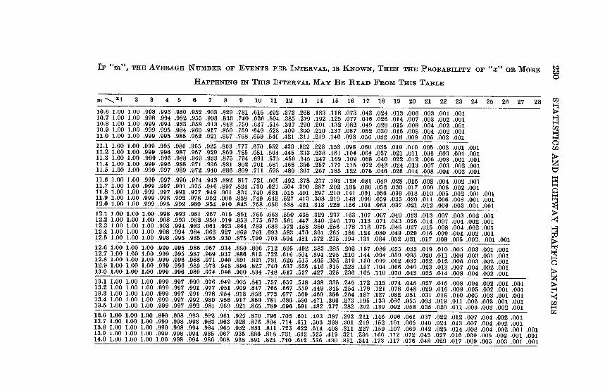
IF "M", THE AVERAGE NumBER OF EvENTs P:m INTERVAL, is Ki-TowN, THEN THE PROBABILITY OF "X" OR MORE
H-A-PPENING IN THis INTERVAL MAY BF, READ FRom THis TA13LE
M -' X1 2 3 4 5 6 7 8 9 10 11 12 13 14 15 16 17 18 19 20 21 22 23 24 25 26 27 28
10.6 1.00 1.00 10.7 1.00 1.00 10.8 1.00 1.00 10.0 1.00 1.00 11.0 1.00 1.00
.998 .993 .980 .952 .903 .829 .731 .616 .492 .373 .268 .183 .118 .073 .043
.998 .994 .982 .955 .908 .836 .740 .626 .604: .385 .2719 .192 .125 .077 .046
.909 .994 .983 .958 .913 .843 .750 .637 .516 .397 .290 .201 .132 .082 .049
.999 .995 .984 .960 .917 .860 .759 -649 .526 .400 .300 .210 .137 .087 .052
.999 .095 .985 .962 .921 .867 .768 .659 .54C .421 .311 .219 .146 .093 .056
.024 .013 .006 .003 .001 .001
.026 .014 .007 .003 .002 .001
.028 .015 .008 .004 .002 .001
.030 .016 .008 .004 .002 .001
.032 .018 .009 .005 .002 .001
m
11.1 1.00 11.2 1.00 11.3 1.00 11.4 1.00 11.5 1.00
1.00 .999 .995 .086 .965 .925 .863 .777 .670 1.00 .990 .996 .087 .967 .929 .869 .785 .681 1.00 .999 .996 .988 .969 .933 .875 .794 .691 1.00 .999 .996 .988 .971 .936 .881 .802 .701 1.00 .999 .997 .989 .972 .940 .886 .809 .711
.552 .433 .322 .228 .153 .098 .060 .035 .019 .010 .005 .003 .001 .001
.664 .445 .333 .238 .161 .104 .064 .037 .021 .011 .006 .003 .001 .001 .67,1, .456 .345 .247 .169 .109 .068 .040 .022 .012 .006 .003 .001 .001 .58i .468 .356 .257 .177 .115 -072 .043 .024 .013 .007 .003 .002 .001 .59E, .480 .367 .267 .185 .122 .076 .046 .026 .014 .008 .004 .002 .001 tj
11.6 1.00 11.7 1.00 11.8 1.00 11.9 1.00 12.0 1.00
1.00 1.00 1.00 1.00 1.00
.999 ;997 .990 .974 .943 .892 .817 .721 .60C .492 .378
.999 .997 .991 .975 .946 .897 .824 .730 .621 .504 .390
.999 .997 .991 .977 .949 .901 .831 .740 .631 .516 .401
.999 .998 .992 .978 .952 .906 .838 .749 .642 .527 .41.3
.099 .998 .992 .980 .954 .910 .845 .758 .653 .538 .424
.277
.287 .297 .308 .318
.103 .128 .081 .049 .028 .016 .008
.202 .135 .086 .052 .030 .017 .009
.210 .141 .091 .056 .033 .018 .010
.219 .148 .096 .059 .035 .020 .011
.228 .156 .101 .063 .037 .021 .012
.004 .002 .001
.005 .002 .001
.005 .002 .001 .001
.006 .003 .001 .001
.006 .003 .001 .001
12.1 12.2 12.3 12.4 12.5
1.00 1.00 1.00 1.00 1.00 1.00 1.00 1.00 1.00 1.00 1.00 1.00 1.00 1.00 1.00
.998 .993 .981 .957 .916 .851
.998 .993 .982 .959 .919 .858
.998 .994 .9S3 .961 .923 .864
.998 .994 .984 .963 .927 .869
.998 .995 .985 .965 .930 .875
.766 .663 .550 .435
.775 .673 .561 .447
.783 .683 .572 .458
.791 .693 .583 .470
.799 .703 .594 .481
.329 .237 .163 .107 .067 .040 .023 .013 .007 .003 .002 .001
.340 .246 .170 .113 .071 .043 .025 .014 .007 .004 .002 .001
.350 .256 .178 .118 .075 .046 .027 .015 .008 .004 .002 .001
.361 .265 .186 .124 .080 .049 .029 .016 .009 .004 .002 .001
.372 .275 .194 .131 .084 .062 .031 .017 .009 .005 .002. .001 .001
12.6 12.7 12.8 12.9 13.0
1.00 1.00 1.00 1.00 1.00 1.00 1.00 1.00 1.00 1.00
1.00 .999 .995 1.00 .099 .995 1.00 .999 .096 1.00 .099 .996 1.00 .999 .996
.986 .967 .934 .880
.987 .069 .937 .886
.988 .971 .940 .891
.989 .973 .943 .896
.989 .974 .946 .900
.806 .712 .605 .492
.813 .722 .616 .504
.821 .731 .626 .515
.827 .740 .637 .526
.834 .748 .647 .537
.383 .285
.394 .295
.405 .305
.416 .315
.427 .325
.202 .137
.210 .144
.219 .160
.228 .157
.236 .165
.089 .055 .033 .019
.094 .059 -035 .020
.099 .062 .037 .022
.104 .066 .040 .023
.110 .070 .043 .025
.010
.011
.012
.013
.014
.005 .003 .001 .001
.006 .003 .001 .001
.006 .003 .002 .001
.007 .004 .002 .001
.008 .004 .002 .001
13.1 1.00 1.00 1.00 .999 13.2 1.00 1.00 1.00 .999 13.3 1.00 1.00 1.00 .999 13.4 1.00 1.00 1.00 .999 13.5 1.00 1.00 1.00 .999
.997 .900
.997 .991
.997 .991
.997 .902
.997 .992
.976 .940
.977 .951
.978 .954
.080 .956
.981 .959
.905 .841
.909 .847
.913 .853
.917 .859
.921 .865
.767 .657 .548
.765 .667 .559
.773 .677 .569
.781 .686 .580
.789 .696 .591
.438 .335 .245 .172 .115 .074 .045 .027 .015 .008 .004 .002 .001 .001
.449 .345 .254 .179 .121 .078 .048 .029 .016 .009 .005 .002 .001 .001 .460 .356 .264 .187 .127 .082 .051 .031 .018 .010 .005 .003 .001 .001 .471 .366 .273 .195 .133 .087 .055 .033 .019 .011 .006 .003 .001 .001 .482 .377 .282 .202 .139 .092 .058 .035 .020 .011 .006 .003 .002 .001
13.6 1.00 13.7 1.00 13.8 1.00 13.9 1.00 14.0 1.00
1.00 1.00 .999 .998 .993 .982 .961 .925 .870 .796 .705 .601 .493 .387 .292 .211 1.00 1.00 .999 .998 .993 .983 .963 .928 .876 .804 .714 .611 .503 .398 .301 .219 1.00 1.00 .999 .998 .994 .984 .965 .932 .881 .811 .723 .622 .514 .408 .311 .227 1.00 1.00 .909 .998 .904 .985 .967 .935 .886 .818 .731 .632 .525 .419 .321 .235 1.00 1.00 1.00 .998 .994 .086 .968 .938 .891 .824 .740 .642 .536 .430 .331 .244
.146 .096 .061 .037 .022 .012 .007 .004 .002 .001
.152 .101 .065 .040 .024 .013 .007 .004 .002 .001
.159 .107 .060 .042 .025 .014 .008 .004 .002 .001 .001
.166 .112 .072 .045 .027 .016 .009 .005 .002 .001 .001
.173 .117 .076 .048 .029 .017 .009 .005 .003 .001 .001

IF "M", THE AVERAGE NUA113ER OF EVENTS PER INTERVAL, is KNOWN, THEN THE PROBABILITY OF "X" OR MORE
HAPPENING IN THIS INTERVAL MAY BE READ FRom Tins TABLE
m 1 2 a 4 5 6 7 8 9 10 11 12 13 14 15 16 17 18 19 20 21 22 23 24 25 26 27 28 29
14.1 1.00 1.00 1.00 1.00 .998 .995 .987 .970 .941 .895 .831 .748 .651 .546 .440 .341 .253 .180 .123 .081 .051 .031 .018 .010 .005 .003 .001 .00114.2 1.00 1.00 1.00 1.00 .998 .995 .987 .972 .944 .900 .837 .756 .661 .557 .451 .351 .262 .187 .129 .085 .054 .033 .019 .011 .006 .003 .002 .00114.3 1.00 1.00 1.00 1.00 .999 .995 .988 .973 .047 .904 .843 .764 .670 .567 .461 .361 .271 .195 .135 .089 .057 .035 .021 .012 .006 .003 .002 .00114.4 1.00 1.00 1.00 1.00 .999 .996 .989 .975 .949 .908 .849 .772 .680 .577 .472 .371 .280 .203 .141 .094 .060 .037 .022 .013 .007 .004 .002 .00114.5 1.00 1.00 1.00 1.00 .999 .996 .990 .976 .952 .912 .855 .780 .689 .587 .482 .381 .289 .210 .147 .099 .064 .040 .024 .014 .008 .004 .002 .001 .001
14.6 1.00 1.00 1.00 1.00 .999 .996 .990 .977 .954 .916 .861 .787 .698 .598 .493 .391 .298 .218 .153 .104 .067 .042 .025 .015 .008 .004 .002 .001 .00114.7 1.00 1.00 1.00 1.00 .999 .997 .991 .979 .956 .920 .866 .795 .707 .608 .503 .401 .307 .226 .160 .109 .071 .045 .027 .016 .009 .005 .003 .001 .00114.8 1.00 1.00 1.00 1.00 .999 .997 .991 .980 .958 .923 .871 .802 .715 .617 .514 .411 .317 .234 .167 .114 .075 .047 .029 .017 .010 .005 .003 .001 .00114.9 1.00 1.00 1.00 1.00 .999 .997 .992 .981 .961 .927 .877 .809 .724 .627 .524 .422 .326 .243 .174 .119 .079 .050 .031 .018 .010 .006 .003 .002 .00115.0 1.00 1.00 1.00 1.00 .999 .997 .992 .982 .963 .930 .882 .815 .732 .638 .534 .432 .336 .251 .181 .125 .083 .053 .033 .019 .011 .006 .003 .002 .001
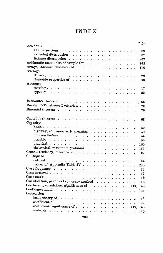
INDEX
Page, Accidents
at intersections . . . . . . . . . . . . . . . . . . . . . 209expected distribution . . . . . . . . . . . . . . . . . . 207Poisson distribution . . . . . . . . . . . . . . . . . . . 207
Arithmetic mean, size of sample for . . . . . . . . . . . . . . 145Arrays, standard deviation of . . . . . . . . . . . . . . . . . 116Average
defined . . . . . . . . . . . . . . . . . . . . . . . . . 22desirable properties of . . . . . . . . . . . . . . . . . . 58
Averagesmoving . . . . . . . . . . . . . . . . . . . . . . . . . 17typesof . . . . . . . . . . . . . . . . . . . . . . . . 22
Bernoulli's theorem . . . . . . . . . . . .. . . . . . . . . 65, 66Bienaym6-Tchebyeheffcriterion . . . . . . . . . . . . . . . . 70Binomial theorem . . . . . . . . . . . . . . . . . . . . . . 75
Cantelli's theorem . . . . . . . . . . . . . . . . . . . . . . 68Capacity
basic . . . . . . . . . . . . . . . . . . . . . . . . . . 150highway, confusion as to meaning . . . . . . . . . . . . . 160limitinL7 factors . . . . . . . . . . . . . . . . . . . . . 1.54
possible . . . . . . . . . . . . . . . . . . . . . . . . 150practical . . . . . . . . . . . . . . . . . . . . . . . . 150theoretical, maximum (volume) . . . . . . . . . . . . . . 151
Central tendency, measure of . . . . . . . . . . . . . . . . . 27Chi-Square
defined . . . . . . . . . . . . . . . . . . . . . . . . . 104values of, Appendix Table IV . . . . . . . . . . . . . . . 220
Class frequency . . . . . . . . . . . . . . . . . . . . . . . 12Class interval . . . . . . . . . . . . . . . . . . . . . . . . 12Class mark . . . . . . . . . . . . . . . . . . . . . . . . . 12Classification, graphical summary method . . . . . . . . . . . 15Coefficient, correlation, significance of . . . . . . . . . . . 147, 148Confidence limits . . . . . . . . . . . . . . . . . . . . . . 142Correlation
basic theory of . . . . . . . . . . . . . . . . . . . . . 113coefficient of . . . . . . . . . . . . . . . . . . . . . . 107coefficient, significance of . . . . . . . . . . . . . . . 147, 148multiple . . . . . . . . . . . . . . . . . . . . . . . . 120
232

INDEX 233 Page
multiple, example of . . . . . . . . . . . . . . . . . . . 121partial . . . . . . . . . . . . . . . . . . . . . . . . . 125ratio . . . . . . . . . . . . . . . . . . . . . . . . . . 117simple, of driver tests . . . . . . . . . . . . . . . . . . 122
Crossing streams of traffic . . . . . . . . . . . . . . . . . . 189Curves
cumulative frequency . . . . . . . . . . . . . . . . . . 19frequency . . . . . . . . . . . . . . . . . . . . . . . 18probability, areas under the normal, Appendix Table I . . . . 217
Delay at signalized intersections, calculating . . . . . . . . . . 203Delay, average arrival method of determining . . . . . . . . . . 206Determinants, evaluation of . . . . . . . . . . . . . . . . . 134Deviation
average . . . . . . . . . . . . . . . . . . . . . . . . 51mean . . . . . . . . . . . . . . . . . . . . . . . . . 51of arrays, standard . . . . . . . . . . . . . . . . . . . 116standard . . . . . . . . . . . . . . . . . . . . . . . . 45
Dispersion and Variance . . . . . . . . . . . . . . . . . . . 97Distribution
binomial, arithmetic mean of . . . . . . . . . . . . . . . 80binomial, arithmetic mean of, example . . . . . . . . . . . 80binomial, James Bernoulli, 1700 . . . . . . . . . . . . . 61, 78binomial, modal term of . . . . . . . . . . . . . . . . . 79binomial, modal term of, examples . . . . . . . . . . . . . 79binomial, table . . . . . . . . . . . . . . . . . . . . . 78binomial, variance of . . . . . . . . . . . . . . . . . . . 81elements of . . . . . . . . . . . . . . . . . . . . . . . 61experimental . . . . . . . . . . . . . . . . . . . . . . 63frequency . . . . . . . . . . . . . . . . . . . . . . 12, 22hypergeometric . . . . . . . . . . . . . . . . . . . . . 104hypergeometric, example . . . . . . . . . . . . . . . . . 105interpretation of the properties of normal . . . . . . . . . . 88Laplace and Gauss, 1800 . . . . . . . . . . . . . . . . . 61moments of . . . . . . . . . . . . . . . . . . . . . . . 54multinomial . . . . . . . . . . . . . . . . . . . . . . 102normal, Demoivre, 1700 . . . . . . . . . . . . . . . . 61, 85normal, interpretation of the properties of . . . . . . . . . 88of sample arithmeticmeans . . . . . . . . . . . . . . . . 139Poisson . . . . . . . . . . . . . . . . . . . . . . . . 90Poisson, arithmetic mean of . . . . . . . . . . . . . . . . 93Poisson, sum of the terms of . . . . . . . . . . . . . . . 93Poisson, variance of . . . . . . . . . . . . . . . . . . . 94probability . . . . . . . . . . . . . . . . . . . . . . . 79

234 INDEX Page
relative frequency . . . . . . . . . . . . . . . . . . . . 78sample . . . . . . . . . . . . . . . . . . . . . . . . . 63theoretical . . . . . . . . . . . . . . . . . . . . . . 62, 65
Distribution Theory binomial . . . . . . . . . . . . . . . . . . . . . . . . 61 normal . . . . . . . . . . . . . . . . . . . . . . . . . 61 Poisson . . . . . . . . . . . . . . . . . . . . . . . . 61
Enoscope . . . . . . . . . . . . . . . . . . . . . . . . . . 7 Estimating speeds and volumes . . . . . . . . . . . . . . . . 181 Events
per interval, Appendix Table VI . . . . . . . . . . . . . . 226 rare, accidents at intersections . . . . . . . . . . . . . . 209 rare, accidents . . . . . . . . . . . . . . . . . . . . . 207 universe of . . . . . . . . . . . . . . . . . . . . . . . 61
Expectation . . . mathematical . . . . . . . . . . . . . . . . . . . . . 27, 29 mathematical, of powers of a variable . . . . . . . . . . . 54
Exponential Function, Poisson. . . . . . . . . . . . . . . . 92, 95
F, 5 % and I% points for distribution of, Appendix Table V . . . 222 Frequency
class . . . . . . . . . . . . . . . . . . . . . . . . . . 13cumulative . . . . . . . . . . . . . . . . . . . . . . . 19curve . . . . . . . . . . . . . . . . . . . . . . . . . isdistribution . . . . . . . . . . . . . . . . . . . . . . . 12distributionof speeds . . . . . . . . . . . . . . . . . . 173polygon . . . . . . . . . . . . . . . . . . . . . . . . 17polygon, smoothed . . . . . . . . . . . . . . . . . . . . 17rectangles . . . . . . . . . . . . . . . . . . . . . . . 15relative . . . . . . . . . . . . . . . . . . . . . . . 13, 64
Gap, estimate of size required for weaving . . . . . . . . . . . 187 Goodness of Fit
Chi-square test of . . . . . . . . . . . . . . . . . . . . 104 of the Poisson series, test of . . . . . . . . . . . . . . . . 163 a graphical method of determining . . . . . . . . . . . . . 178
Histogram . .. . . . . . . . . . . . . . . . . . . . . . . . 16
Intersections accidents at . . . . . . . . . . . . . . . . . . . . . . . 209 signalized . . . . . . . . . . . . . . . . . . . . . . . . 198 signalized, calculating delay . . . . . . . . . . . . . . . . 203 traffic performance at urban street . . . . . . . . . . . . 204
Intervals, average length . . . . . . . . . . . . . . . . . . . 194
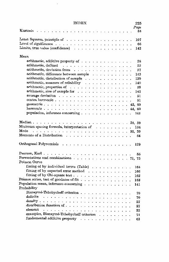
INDEX 235 Page
Kurtosis . . . . . . . . . . . . . . . . . . . . . . . . . . 84
Least Squares, principle of . . . . . . . . . . . . . . . . . . 107Level of significance . . . . . . . . . . . . . . . . . . . . . 66Limits, true value (confidence) . . . . . . . . . . . . . . . . 142
Meanarithmetic, additive property of . . . . . . . . . . . . . . 28arithmetic, defined . . . . . . . . . . . . . . . . . . . 22arithmetic, deviation from . . . . . . . . . . . . . . . . 27arithmetic, difference between sample . . . . . . . . . . . 143arithmetic, distribution of sample . . . . . . . . . . . . . 139arithmetic, measure of reliability . . . . . . . . . . . . . 140arithmetic, propertiesof . . . . . . . . . . . . . . . . . 69arithmetic, size of sample for . . . . . . . . . . . . . . . 145average deviation . . . . . . . . . . . . . . . . . . . . 51centra harmonic . . . . . . . . . . . . . . . . . . . . . 51geometric . . . . . . . . . . . . . . . . . . . . . . . 42, 60harmonic . . . . . . . . . . . . . . . . . . . . . . . 44, 60population, inference concerning . . . . . . . . . . . . . . 141
Median . . . . . . . . . . . . . . . . . . . . . . . . . . 38, 59Minimum spacing formula, interpretationof . . . . . . . . . . 154Mode . . . . . . . . . . . . . . . . . . . . . . . . . . 35, 39Moments of a Distribution . . . . . . . . . . . . . . . . . . 54
Orthogonal Polynomials . . . . . . . . . . . . . . . . . . . 129
Pearson, Karl . . . . . . . . . . . . . . . . . . . . . . . . 55Permutations and combinations . . . . . . . . . . . . . . . 71, 73Poisson. Curve
fitting of by individual terms (Table) . . . . . . . . . . . 164fitting of by expected error method . . . . . . . . . . . . 166fitting of by Chi-square test . . . . . . . . . . . . . . . . 162
P6isson series, test of goodness of fit . . . . . . . . . . . . . . 163Populationmean, inference concerning . . . . . . . . . . . . . 141Probability
Bienaym6-Tchebyeheffcriterion . . . . . . . . . . . . . . 70definite . . . . . . . . . . . . . . . . . . . . . . . . 70density . . . . . . . . . . . . . . . . . . . . . . . . . 22distribution function of . . . . . . . . . . . . . . . . . . 22element . . . . . . . . . . . . . . . . . . . . . . . . 22examples, Bienaym6-Tchebycheffcriterion . . . . . . . . . 71fundamental additive property . . . . . . . . . . . . . . 63
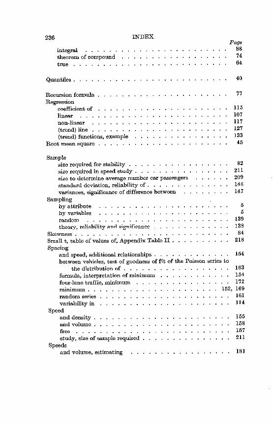
236 INDEX Page
integral . . . . . . . . . . . . . . . . . . . . . . . . 88theorem of compound . . . . . . . . . . . . . . . . . . 74true . . . . . . . . . . . . . . . . . . . . . . . . . . 64
Quantiles . . . . . . . . . . . . . . . . . . . . . . . . . . 40
Recursion formula . . . . . . . . . . . . . . . . . . . . . . 77Regression
coefficient of . . . . . . . . . . . ... . . . . . . . . . 115linear . . . . . . . . . . . . . . . . . . . . . . . . . 107non-linear . . . . . . . . . . . . . . . . . . . . . . . 117(trend) line . . . . . . . . . . . . . . . . . . . . . . . 127(trend) functions, example . . . . . . . . . . . . . . . . 133
Root mean square . . . . . . . . . . . . . . . . . . . . . . 45
Samplesize required for stability . . . . . . . . . . . . . . . . . 82size required in speed study . . . . . . . . . . . . . . . . 211size to determine average number car passengers . . . . . . 209standard deviation, reliability of . . . . . . . . . . . . . . 146variances, significance of difference between . . . . . . . . 147
Samplingby attribute . . . . . . . . . . . . . . . . . . . . . . 5by variables . . . . . . . . . . . . . . . . . . . . . . 5random . . . . . . . . . . . . . . . . . . . . . . . . 139theory. reliability send qium-ifie.A."ce . . . . . . . . . . . . . 1,38
Skewness . . . . . . . . . . . . . . . . . . . . . . . . . . 84Small t, table of values of, Appendix Table II . . . . . . . . . . 218Spacing
and speed, additionalrelationships . . . . . . . . . . . . . 154between vehicles, test of goodness of fit of the Poisson series to
the distribution of . . . . . . . . . . . . . . . . . . 163formula., interpretationof minimum . . . . . . . . . . . . 154four-lane traffic, minimum . . . . . . . . . . . . . . . . 172minimum . . . . . . . . . . . . . . . . . . . . . . 15% 169random series . . . . . . . . . . . . . . . . . . . . . . 161variabilityin . . . . . . . . . . . . . . . . . . . . . . 114
Speedand density . . . . . . . . . . . . . . . . . . . . . . . 155and volume . . . . . . . . . . . . . . . . . . . . . . . 158free . . . . . . . . . . . . . . . . . . . . . . . . . . 157study, size of samplerequired . . . . . . . . . . . . . . . 211
Speedsand volume, estimating . . . . . . . . . . . . . . . . . 181

INDEX 237 Page
calculation of standard deviation of . . . . . . . . . . . . 175 fitting of normal curve to distributionof, Chi-square method . 176 frequency distribution of . . . . . . . . . . . . . . . . . 173
Stability, size of sample required for . . . . . . . . . . . . . . 82 Statistics
and mathematics . . . . . . . . . . . . . . . . . . . . 3 categories . . . . . . . . . . . . . . . . . . . . . . . 4 defined . . . . . . . . . . . . . . . . . . . . . . . . . 3 methods . . . . . . . . . . . . . . . . . . . . . . . . 1 nature . . . . . . . . . . . . . . . . . . . . . . . . . 3 provision of techniques for making inferences . . . . . . . . 138 variables in . . . . . . . . . . . . . . . . . . . . . . . 3
Stochastic, variable . . . . . . . . . . . . . . . . . . . . . 3 Summary numbers, defined . . . . . . . . . . . . . . . . . . 12
Tendency, central, measure of . . . . . . . . . . . . . . . . . 27 Theorem
Bernoulli's . . . . . . . . . . . . . . . . . . . . . . 65, 66binomial . . . . . . . . . . . . . . . . . . . . . . . . 75Cantelli's . . . . . . . . . . . . . . . . . . . . . . . . 68
Time mathematical determinationof vehicle delay . . . . . . . . 190 gaps, graphical method of determining proportion . . . . . . 192
Traffic crossing streams of . . . . . . . . . . . . . . . . . . . 189 the nature of problems of highway . . . . . . . . . . . . . 160
Trend, linear . . . . . . . . . . . . . . . . . . . . . . . . 107
Valueexpected, example . . . . . . . . . . . . . . . . . . . . 30expected, theorem . . . . . . . . . . . . . . . . . . . . 31mean, defined . . . . . . . . . . . . . . . . . . . . . . 33median . . . . . . . . . . . . . . . . . . . . . . . . . 38mode or modal . . . . . . . . . . . . . . . . . . . . . 35
Variable mathematical expectation or expected value of . . . . . . . 27 means of measuring . . . . . . . . . . . . . . . . . . . 6 stochastic . . . . . . . . . . . . . . . . . . . . . . 3, 70
Variability, coefficient of . . . . . . . . . . . . . . . . . . . 51Variance
analysis of . . . . . . . . . . . . . . . . . . . . . . . 120defined . . . . . . . . . . . . . . . . . . . . . . . . . 48dispersion and . . . . . . . . . . . . . . . . . . . . . 97of Poisson distribution . . . . . . . . . . . . . . . . . . 94
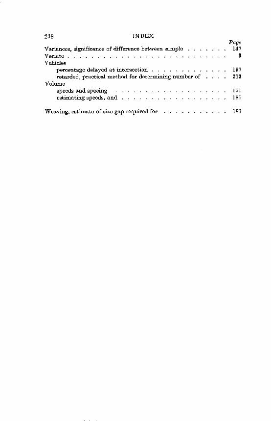
238 INDEX Page
Variances, significance of difference between sample . . . . . . . 147Variate . . . . . . . . . . . . . . . . . . . . . . . . . . . 3Vehicles
percentage delayed at intersection . . . . . . . . . . . . . 197retarded, practical method for determining number of . . . . 203
Volumespeeds and spacing . . . . . . . . . . . . . . . . . . . 151estimating speeds, and . . . . . . . . . . . . . . . . . . 181
Weaving, estimate of size gap required for . . . . . . . . . . 187
v. P y 6 8 C
. q
0 t x A /Z v
o n Q
Alpha Beta Gamma Delta Epsilon Zeta Eta
Theta Iota Kappa Lambda Mu Nu xi Omicron Pi Rho
a or.5 Sigma -r v 99 X TP co
Tau Upsilon Phi Chi Psi Omega
Related Documents