Highly Accurate Method for Real-Time Active Power Reserve ...

NREL is a national laboratory of the U.S. Department of Energy Office of Energy Efficiency & Renewable Energy Operated by the Alliance for Sustainable Energy, LLC This report is available at no cost from the National Renewable Energy Laboratory (NREL) at www.nrel.gov/publications.

Contract No. DE-AC36-08GO28308

Conference Paper NREL/CP-5D00-72419 June 2019

Highly Accurate Method for Real-Time Active Power Reserve Estimation for Utility-Scale PV Power Plants Preprint Vahan Gevorgian

National Renewable Energy Laboratory

Presented at the Solar Integration Workshop Stockholm, Sweden October 16-17, 2018

NREL is a national laboratory of the U.S. Department of Energy Office of Energy Efficiency & Renewable Energy Operated by the Alliance for Sustainable Energy, LLC This report is available at no cost from the National Renewable Energy Laboratory (NREL) at www.nrel.gov/publications.

Contract No. DE-AC36-08GO28308

National Renewable Energy Laboratory 15013 Denver West Parkway Golden, CO 80401 303-275-3000 • www.nrel.gov

Conference Paper NREL/CP-5D00-72419 June 2019

Highly Accurate Method for Real-Time Active Power Reserve Estimation for Utility-Scale PV Power Plants Preprint Vahan Gevorgian

National Renewable Energy Laboratory

Suggested Citation Gevorgian, Vahan. 2019. Highly Accurate Method for Real-Time Active Power Reserve Estimation for Utility-Scale PV Power Plants: Preprint. Golden, CO: National Renewable Energy Laboratory. NREL/CP-5D00-72419. https://www.nrel.gov/docs/fy19osti/72419.pdf.

NOTICE

This work was authored by the National Renewable Energy Laboratory, operated by Alliance for Sustainable Energy, LLC, for the U.S. Department of Energy (DOE) under Contract No. DE-AC36-08GO28308. Funding provided by the U.S. Department of Energy Office of Energy Efficiency and Renewable Energy Solar Energy Technologies Office. The views expressed herein do not necessarily represent the views of the DOE or the U.S. Government.

This report is available at no cost from the National Renewable Energy Laboratory (NREL) at www.nrel.gov/publications.

U.S. Department of Energy (DOE) reports produced after 1991 and a growing number of pre-1991 documents are available free via www.OSTI.gov.

Cover Photos by Dennis Schroeder: (clockwise, left to right) NREL 51934, NREL 45897, NREL 42160, NREL 45891, NREL 48097, NREL 46526.

NREL prints on paper that contains recycled content.

1 This report is available at no cost from the National Renewable Energy Laboratory (NREL) at www.nrel.gov/publications.

Highly Accurate Method for Real-Time Active Power Reserve Estimation for Utility-Scale PV Power Plants

Vahan Gevorgian National Renewable Energy Laboratory (NREL)

Golden, Colorado, USA [email protected]

Abstract— This paper applies a robust technique for determining the available power reserve from a curtailed utility-scale photovoltaic (PV) power plant. The proposed technique does not require deploying any additional equipment or sensors and is based only on the addition of new control logic to the existing power plant controller. Also, the proposed method is universally applicable to PV plants with any type of smart inverters and PV modules. Accurate determination of available power is important for using curtailed PV generation as a resource for various types of active power controls, such as spinning reserves and primary and secondary frequency control. For PV plants to be able to maintain the desired regulation range, the plant controller must be able to estimate the available aggregate peak power that all the plant’s inverters can produce at any point in time and ensure that the control error stays within the tolerance band at all times. In this paper, we explore a highly accurate control method that uses dedicated inverters within the plant as reference units and evaluates the available aggregate peak power for the whole plant under different cloud variability conditions.

Keywords-component; Photovoltaics; Active power control style; Power reserves; Maximum power point estimation

I. INTRODUCTION All over the world, system operators and utilities are

continually adapting their grid codes, interconnection requirements, operational practices, and market mechanisms to make the integration of shares of fast-growing variable renewable generation both reliable and economic [1]. As power system continues to evolve, the Federal Energy Regulatory Commission (FERC) noted that there is a growing need for a refined understanding of the services necessary to maintain a reliable and efficient system. In orders 755 and 784, FERC required improving the mechanisms by which frequency regulation service is procured and enabling compensation by fast-response resources such as energy storage. In addition, FERC recently issued a notice of proposed rulemaking to enable aggregation of distributed storage and distributed generation [2]. The North American Electric Reliability Corporation’s (NERC) Integration of Variable Generation Task Force made several

recommendations for requirements for variable generators (including solar) to provide their share of grid support, including active power control (APC) capabilities [3], [4]. Similar requirements for renewable energy plants have been introduced in Europe at both the transmission and distribution levels [5], [6]. In 2018, FERC Order No. 842 amended the pro forma interconnection agreements to include certain operating requirements, including maximum droop and deadband parameters, and sustained response provisions [7].

NERC’s BAL-003-1 Standard on Frequency Response and Frequency Bias Setting establishes target contingency protection criteria for each North American interconnection and individual balancing authorities (BAs) within interconnections [8]. BAs need to meet a minimum frequency response obligation (FRO), so the generating resources that are operated in a mode and range to meet their FRO need to have adequate headroom to respond to frequency transients and load-frequency control set points. Establishing this headroom is not a problem for the conventional generation fleet, but the varying nature of solar and wind generation makes it challenging to set and maintain adequate headroom for these varying resources. In general, all system operators have processes and procedures in place to ensure grid reliability by monitoring market participant operation. For example, provisions of the California Independent System Operator (CAISO) tariff [9] sets penalties for deviations from dispatch and regulation capacity for market participants that fail to comply. The permitted area of variation for performance requirements of resources used for various purposes is provided in the CAISO tariff [9]. The tolerance band is expressed in terms of energy (MWh) for generating units and imports from external dynamic system resources for each settlement interval, and it equals the greater of the absolute value calculated using either of the following methods: (1) 5 MW divided by the number of settlement intervals per settlement period; (2) 3% of the relevant generating unit’s maximum output (Pmax), as registered in the master file, divided by the number of settlement intervals per settlement period.

This CAISO tariff and similar requirements from other system operators imply that the accurate real-time estimation of available maximum power from a curtailed photovoltaic

2 This report is available at no cost from the National Renewable Energy Laboratory (NREL) at www.nrel.gov/publications.

(PV) plant is important for avoiding excessive penalty payments if utility-scale PV plants become market participants for energy and various reliability services related to active power controls.

A typical modern utility-scale PV power plant is a complex system of large PV arrays and multiple power electronic inverters, and it can contribute to mitigating the impacts on grid stability and reliability through sophisticated automatic “grid-friendly” controls. To provide active power reserves (or a headroom margin) for up-regulation that can be automatically dispatched as needed, a PV plant needs to operate below its maximum power point (MPP); however, evaluating that MPP in curtailed mode is not a trivial task, especially for large PV power plants during various types of variable conditions caused by clouds. One paper [10] proposed an experimentally validated maximum power point estimation (MPPE) method, which operates in real time using irradiance and cell temperature measurements to ensure that sufficient reserve power is available. Another paper [11] proposes an advanced real-time MPP estimation algorithm by applying curve fitting on voltage and current measurements obtained during inverter operation. Some previously proposed MPPE methods used offline prediction and employed regression analysis or neural networks [12], [13]. These methods seem to be accurate but might require excessive processing power. Others have proposed methods for real-time calculation ([14]– [16]) by making assumptions that reduce the accuracy of the PV model or, in some cases, require knowledge that is not typically available on PV module data sheets[14], [17]. Another important limitation of MPPE estimation methods is that modifications are needed based on inverter types and topologies. For example, in single-stage inverters (no DC/DC conversion), the power reserve capability can be achieved by inverter control modifications [18], [19]; however, in two-stage systems (inverter and DC/DC converter), the DC/DC converter control needs to be modified [20]. This makes the use of maximum peak power estimation for curtailed PV systems challenging and highly dependent on inverter make and topology, types of modules used in PV plants, and accurate knowledge of inverter and PV module parameters.

The variability of solar PV output in the regulation reserve time frame among various arrays within a large-scale (~50 MW) solar PV plant in the southwestern United States was explored in [21]. Although the distributions of changes in aggregate power output throughout all timescales considered were clustered around a strong peak at zero, the distributions at all timescales exhibited significant instances of higher magnitude ramps in the tails of the histograms. The results achieved in [21] were very important because the method presented in this paper was also tested using the data from the same PV power plant.

In 2015, a demonstration project was conducted in the U.S. territory of Puerto Rico using a 20-MW grid-connected PV power plant [22]. This plant was controlled to provide different types of reliability services to the island’s grid, including various types of active power controls. Testing on this plant provided “real-world” data on levels of uncertainty that can be introduced by traditional MPPE estimation methods based on irradiance and temperature measurements

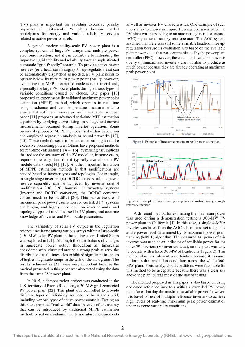
as well as inverter I-V characteristics. One example of such uncertainty is shown in Figure 1 during operation when the PV plant was responding to an automatic generation control AGC) signal sent from system operator. The AGC system assumed that there was still some available headroom for up-regulation because its evaluation was based on the available plant power value that was communicated by the power plant controller (PPC); however, the calculated available power is overly optimistic, and inverters are not able to produce as much power because they are already operating at maximum peak power point.

Figure 1. Example of inaccurate maximum peak power estimation

Figure 2. Example of maximum peak power estimation using a single reference inverter

A different method for estimating the maximum power was used during a demonstration testing a 300-MW PV power plant in California [1]. In this case, a single 4-MVA inverter was taken from the AGC scheme and set to operate at the power level determined by its maximum power point tracking (MPPT) algorithm. The measured AC power of this inverter was used as an indicator of available power for the other 79 inverters (80 inverters total), so the plant was able to operate with a fixed 30 MW of headroom (Figure 2). This method also has inherent uncertainties because it assumes uniform solar irradiation conditions across the whole 300-MW plant. Fortunately, cloud conditions were favorable for this method to be acceptable because there was a clear sky above the plant during most of the day of testing.

The method proposed in this paper is also based on using dedicated reference inverters within a curtailed PV power plant for estimating the maximum available power; however, it is based on use of multiple reference inverters to achieve high levels of real-time maximum peak power estimation under extreme variability conditions.

3 This report is available at no cost from the National Renewable Energy Laboratory (NREL) at www.nrel.gov/publications.

II. PROPOSED METHOD For utility-scale PV power plants to be able to maintain

the desired regulation range or spinning reserve levels, the plant controller must be able to estimate the available aggregate peak power that all the plant’s inverters can produce at any point in time. The available power is normally estimated by an algorithm that considers solar irradiation, PV modules I-V characteristics and temperatures, inverter efficiencies, etc.; however, this method has many uncertainties, depends on the availability of accurate system models, and does not account for other factors, such as panel soiling because of dust. The proposed method can determine the available peak power of the PV plant and maintain desired reserves with high levels of accuracy without the use of external sensors or devices. The existing plant hardware and controls can perform this task after the addition of the new optimized control algorithm in the power plant controller software.

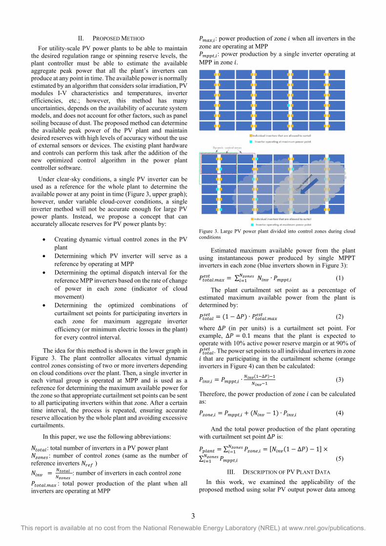
Under clear-sky conditions, a single PV inverter can be used as a reference for the whole plant to determine the available power at any point in time (Figure 3, upper graph); however, under variable cloud-cover conditions, a single inverter method will not be accurate enough for large PV power plants. Instead, we propose a concept that can accurately allocate reserves for PV power plants by:

• Creating dynamic virtual control zones in the PV

plant • Determining which PV inverter will serve as a

reference by operating at MPP • Determining the optimal dispatch interval for the

reference MPP inverters based on the rate of change of power in each zone (indicator of cloud movement)

• Determining the optimized combinations of curtailment set points for participating inverters in each zone for maximum aggregate inverter efficiency (or minimum electric losses in the plant) for every control interval.

The idea for this method is shown in the lower graph in Figure 3. The plant controller allocates virtual dynamic control zones consisting of two or more inverters depending on cloud conditions over the plant. Then, a single inverter in each virtual group is operated at MPP and is used as a reference for determining the maximum available power for the zone so that appropriate curtailment set points can be sent to all participating inverters within that zone. After a certain time interval, the process is repeated, ensuring accurate reserve allocation by the whole plant and avoiding excessive curtailments.

In this paper, we use the following abbreviations:

𝑁𝑁𝑡𝑡𝑡𝑡𝑡𝑡𝑡𝑡𝑡𝑡: total number of inverters in a PV power plant 𝑁𝑁𝑧𝑧𝑡𝑡𝑧𝑧𝑧𝑧𝑧𝑧 : number of control zones (same as the number of reference inverters 𝑁𝑁𝑟𝑟𝑧𝑧𝑟𝑟 ) 𝑁𝑁𝑖𝑖𝑧𝑧𝑖𝑖 = 𝑁𝑁𝑡𝑡𝑡𝑡𝑡𝑡𝑡𝑡𝑡𝑡

𝑁𝑁𝑧𝑧𝑡𝑡𝑧𝑧𝑧𝑧𝑧𝑧 : number of inverters in each control zone

𝑃𝑃𝑡𝑡𝑡𝑡𝑡𝑡𝑡𝑡𝑡𝑡.𝑚𝑚𝑡𝑡𝑚𝑚 : total power production of the plant when all inverters are operating at MPP

𝑃𝑃𝑚𝑚𝑡𝑡𝑚𝑚,𝑖𝑖: power production of zone 𝑖𝑖 when all inverters in the zone are operating at MPP 𝑃𝑃𝑚𝑚𝑚𝑚𝑚𝑚𝑡𝑡,𝑖𝑖: power production by a single inverter operating at MPP in zone 𝑖𝑖.

Figure 3. Large PV power plant divided into control zones during cloud conditions

Estimated maximum available power from the plant using instantaneous power produced by single MPPT inverters in each zone (blue inverters shown in Figure 3):

𝑃𝑃𝑡𝑡𝑡𝑡𝑡𝑡𝑡𝑡𝑡𝑡.𝑚𝑚𝑡𝑡𝑚𝑚𝑧𝑧𝑧𝑧𝑡𝑡 = ∑ 𝑁𝑁𝑖𝑖𝑧𝑧𝑖𝑖 ∙ 𝑃𝑃𝑚𝑚𝑚𝑚𝑚𝑚𝑡𝑡,𝑖𝑖𝑁𝑁𝑧𝑧𝑡𝑡𝑧𝑧𝑧𝑧𝑧𝑧 𝑖𝑖=1 (1)

The plant curtailment set point as a percentage of estimated maximum available power from the plant is determined by:

𝑃𝑃𝑡𝑡𝑡𝑡𝑡𝑡𝑡𝑡𝑡𝑡𝑧𝑧𝑧𝑧𝑡𝑡 = (1 − ∆𝑃𝑃) ∙ 𝑃𝑃𝑡𝑡𝑡𝑡𝑡𝑡𝑡𝑡𝑡𝑡.𝑚𝑚𝑡𝑡𝑚𝑚𝑧𝑧𝑧𝑧𝑡𝑡 (2)

where ∆𝑃𝑃 (in per units) is a curtailment set point. For example, ∆𝑃𝑃 = 0.1 means that the plant is expected to operate with 10% active power reserve margin or at 90% of 𝑃𝑃𝑡𝑡𝑡𝑡𝑡𝑡𝑡𝑡𝑡𝑡𝑧𝑧𝑧𝑧𝑡𝑡 . The power set points to all individual inverters in zone 𝑖𝑖 that are participating in the curtailment scheme (orange inverters in Figure 4) can then be calculated:

𝑃𝑃𝑖𝑖𝑧𝑧𝑖𝑖,𝑖𝑖 = 𝑃𝑃𝑚𝑚𝑚𝑚𝑚𝑚𝑡𝑡,𝑖𝑖 ∙𝑁𝑁𝑖𝑖𝑧𝑧𝑖𝑖(1−∆𝑃𝑃)−1

𝑁𝑁𝑖𝑖𝑧𝑧𝑖𝑖−1 (3)

Therefore, the power production of zone 𝑖𝑖 can be calculated as:

𝑃𝑃𝑧𝑧𝑡𝑡𝑧𝑧𝑧𝑧,𝑖𝑖 = 𝑃𝑃𝑚𝑚𝑚𝑚𝑚𝑚𝑡𝑡,𝑖𝑖 + (𝑁𝑁𝑖𝑖𝑧𝑧𝑖𝑖 − 1) ∙ 𝑃𝑃𝑖𝑖𝑧𝑧𝑖𝑖,𝑖𝑖 (4)

And the total power production of the plant operating with curtailment set point ∆𝑃𝑃 is:

𝑃𝑃𝑚𝑚𝑡𝑡𝑡𝑡𝑧𝑧𝑡𝑡 = ∑ 𝑃𝑃𝑧𝑧𝑡𝑡𝑧𝑧𝑧𝑧,𝑖𝑖𝑁𝑁𝑧𝑧𝑡𝑡𝑧𝑧𝑧𝑧𝑧𝑧𝑖𝑖=1 = [𝑁𝑁𝑖𝑖𝑧𝑧𝑖𝑖(1 − ∆𝑃𝑃) − 1] ×

∑ 𝑃𝑃𝑚𝑚𝑚𝑚𝑚𝑚𝑡𝑡,𝑖𝑖𝑁𝑁𝑧𝑧𝑡𝑡𝑧𝑧𝑧𝑧𝑧𝑧𝑖𝑖=1 (5)

III. DESCRIPTION OF PV PLANT DATA In this work, we examined the applicability of the

proposed method using solar PV output power data among

4 This report is available at no cost from the National Renewable Energy Laboratory (NREL) at www.nrel.gov/publications.

different arrays in a single utility-scale (~50 MW) PV plant in the western United States. The plant consists of 96 individual inverters, each rated at 0.5 MW. We use 1-s power data from each individual inverter collected from the plant during a period of several months, allowing us to analyze the accuracy of the proposed method under different resource variability scenarios.

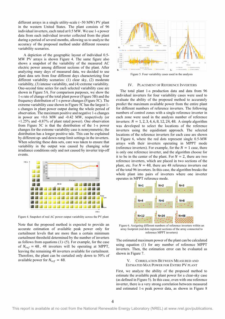
A depiction of the geographic layout of individual 0.5-MW PV arrays is shown Figure 4. The same figure also shows a snapshot of the variability of the measured AC electric power among different sections of the plant. After analyzing many days of measured data, we decided to use plant data sets from four different days characterizing four different variability scenarios: (1) clear sky, (2) moderate variability, (3) intense variability, and (4) extreme variability. One-second time series for each selected variability case are shown in Figure 5A. For comparison purposes, we show the 1-s rate of change of the total plant power (Figure 5B) and the frequency distribution of 1-s power changes (Figure 5C). The extreme variability case shown in Figure 5C has the largest 1-s changes in plant power output during the whole period of observation. The maximum positive and negative 1-s changes in power are +0.6 MW and -0.42 MW, respectively (or +1.25% and -0.87% of plant rated power). One observation from Figure 5C is that the distribution of the 1-s power changes for the extreme variability case is nonsymmetric; the distribution has a longer positive tale. This can be explained by different up- and down-ramp limit settings in the inverters. When selecting these data sets, care was taken to ensure that variability in the output was caused by changing solar irradiance conditions only and not caused by inverter trip-off events.

Figure 4. Snapshot of real AC power output variability across the PV plant

Note that the proposed method is expected to provide an accurate estimation of available peak power only for curtailment levels that are more than a certain minimum curtailment threshold determined by the number of inverters as follows from equations (1)–(5). For example, for the case of 𝑁𝑁𝑟𝑟𝑧𝑧𝑟𝑟 = 48 , 48 inverters will be operating at MPPT, leaving the remaining 48 inverters available for curtailment. Therefore, the plant can be curtailed only down to 50% of available power for 𝑁𝑁𝑟𝑟𝑧𝑧𝑟𝑟 = 48.

Figure 5. Four variability cases used in the analysis

IV. PLACEMENT OF REFERENCE INVERTERS The total plant 1-s production data and data from 96

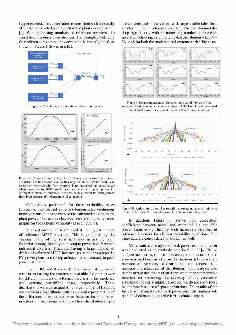
individual inverters for four variability cases were used to evaluate the ability of the proposed method to accurately predict the maximum available power from the entire plant for different numbers of reference inverters. The following numbers of control zones with a single reference inverter in each zone were used in the analysis number of reference inverters: 𝑁𝑁 = 1, 2, 3, 4, 6, 8, 12, 24, 48. A simple algorithm was developed to select the locations of the reference inverters using the equidistant approach. The selected locations of the reference inverters for each case are shown in Figure 6, where the red dots represent single 0.5-MW arrays with their inverters operating in MPPT mode (reference inverters). For example, for the 𝑁𝑁 = 1 case, there is only one reference inverter, and the algorithm choose for it to be in the center of the plant. For 𝑁𝑁 = 2, there are two reference inverters, which are placed in two sections of the plant, etc. For 𝑁𝑁 = 48, there are 48 reference inverters out of the total 96 inverters. In this case, the algorithm breaks the whole plant into pairs of inverters where one inverter operates in MPPT reference mode.

Figure 6. Assigning different numbers of reference inverters within an array footprint (red dots represent sections of the array connected to

reference MPPT inverters)

The estimated maximum power of the plant can be calculated using equation (1) for any number of reference MPPT inverters. Then, the estimation error can be evaluated as shown in Figure 7.

V. CORRELATION BETWEEN MEASURED AND ESTMATED MAX POWER FOR ENTIRE PV PLANT

First, we analyze the ability of the proposed method to estimate the available peak plant power for a clear-sky case (as defined in Figure 5). In this case, even with one reference inverter, there is a very strong correlation between measured and estimated 1-s peak power data, as shown in Figure 8

5 This report is available at no cost from the National Renewable Energy Laboratory (NREL) at www.nrel.gov/publications.

(upper graphs). This observation is consistent with the results of the test conducted on a 300-MW PV plant as described in [1]. With increasing numbers of reference inverters, the correlation becomes even stronger. For example, with only four reference inverters, the correlation is basically ideal, as shown in Figure 8 (lower graphs).

Figure 7. Calculating error in estimated maximum power

Figure 8. Clear-sky case: a high level of accuracy in maximum power evaluation can be achieved even with a single reference inverter, and it can be further improved with four inverters (blue: measured total plant power when operating in MPPT mode; red: estimated total plant power for different numbers of reference inverters, which cannot be distinguished from blue because of high accuracy of estimation)

Calculations performed for three variability cases (moderate, intense, and extreme) demonstrated continuous improvements in the accuracy of the estimated maximum PV plant power. This can be observed from both 1-s time-series graphs for the extreme variability case (Figure 9).

The best correlation is achieved at the highest number of reference MPPT inverters. This is explained by the varying nature of the solar irradiance across the plant footprint causing diversity in the output power level between individual inverters. Therefore, having a larger number of dedicated reference MPPT inverters scattered throughout the PV power plant would help achieve better accuracy in peak power estimation.

Figure 10A and B show the frequency distribution of error in estimating the maximum available PV plant power for different numbers of reference inverters in the moderate and extreme variability cases, respectively. These distributions were calculated for a large number of bins and are shown in a logarithmic scale as a visual representation of the difference in estimation error between the number of inverters and large range of values. These distribution shapes

are concentrated in the center, with large visible tales for a smaller number of reference inverters. The distribution tales drop significantly with an increasing number of reference inverters, achieving essentially no-tail distribution when N = 24 or 48 for both the moderate and extreme variability cases.

Figure 9. Improving accuracy for an extreme variability case (blue:

measured total plant power when operating in MPPT mode; red: estimated total plant power for different numbers of reference inverters)

Figure 10. Reduction of control error with increasing numbers of reference inverters (A: moderate variability case; B: extreme variability case)

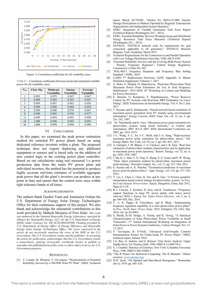
In addition, Figure 11 shows how correlation coefficients between actual and estimated 1-s available power improve significantly with increasing numbers of reference inverters for all four variability conditions. The same data are consolidated in TABLE 1 as well.

More statistical analysis of peak power estimation error was conducted using methods described in [23]– [26] to analyze mean error, standard deviation, min/max errors, and skewness and kurtosis of error distributions (skewness is a measure of symmetry of distribution, and kurtosis is a measure of peakedness of distribution). This analysis also demonstrated the impact of an increased number of reference inverters on improving the accuracy of the estimation statistics of power available; however, we do not show these results here because of space constraints. The results of the full statistical analysis for peak power error distribution will be published in an extended NREL technical report.

A.

B.

Increasing N Increasing N

Increasing N Increasing N

6 This report is available at no cost from the National Renewable Energy Laboratory (NREL) at www.nrel.gov/publications.

Figure 11.Correlation coefficients for all variability cases

TABLE 1. Correlation coefficients between actual and estimated available power for all variability cases

Nref Clear Sky Moderate Variability

Intense Variability

Extreme Variability

1 0.995 0.979 0.947 0.947 2 0.998 0.983 0.955 0.947 3 0.999 0.987 0.963 0.956 4 0.999 0.988 0.968 0.959 6 0.999 0.990 0.974 0.967 8 0.999 0.992 0.976 0.977 12 0.999 0.994 0.992 0.990 24 1.000 0.998 0.995 0.995 48 1.000 0.999 0.998 0.998

VI. CONCLUSIONS In this paper, we examined the peak power estimation

method for curtailed PV power plants based on using dedicated reference inverters within a plant. The proposed technique does not require deploying any additional equipment or sensors and is based only on the addition of new control logic to the existing power plant controller. Based on our calculations using real measured 1-s power production data from the entire PV power plant and individual inverters, the method has the potential to produce highly accurate real-time estimates of available aggregate peak power that all the plant’s inverters can produce at any point in time and ensure that the control error stays within tight tolerance bands at all times.

ACKNOWLEDGMENTS The authors thank Guohui Yuan and Anastasios Golnas the U.S. Department of Energy Solar Energy Technologies Office for their continuous support of this project. We also thank and acknowledge the substantial contributions to this work provided by Mahesh Morjaria of First Solar. This work was authored by the National Renewable Energy Laboratory, operated by Alliance for Sustainable Energy, LLC, for the U.S. Department of Energy (DOE) under Contract No. DE-AC36-08GO28308. Funding provided by U.S. Department of Energy Office of Energy Efficiency and Renewable Energy Solar Energy Technologies Office. The views expressed in the article do not necessarily represent the views of the DOE or the U.S. Government. The U.S. Government retains and the publisher, by accepting the article for publication, acknowledges that the U.S. Government retains a nonexclusive, paid-up, irrevocable, worldwide license to publish or reproduce the published form of this work, or allow others to do so, for U.S. Government purposes.

REFERENCES [1] C. Loutan, M. Morjaria, V. Gevorgian, “Demonstration of Essential

Reliability Services by a 300-MW Solar PV Plant”, NREL Technical

report, March 2017FERC, “Docket No. RM16-23-000: Electric Storage Participation in Markets Operated by Regional Transmission Organizations and Independent System Operators.”

[2] NERC, Integration of Variable Generation Task Force Report (Technical Report) (Washington, D.C.: 2012).

[3] NERC, Essential Reliability Services Working Group and Distributed Energy Resources Task Force Measures (Technical Report) (Washington, D.C.: 2012),

[4] ENTSO-E, “ENTSO-E network code for requirements for grid connection applicable to all generators,” ENTSO-E, Brussels Belgium, Tech. Guideline, March 2013

[5] Technical Requirements for the Connection to and Parallel Operation with Low-Voltage Distribution Networks, VDE-AR-N 4105

[6] “Essential Reliability Services and the Evolving Bulk-Power System – Primary Frequency Response”, Federal Energy Regulatory Commission’s Order No. 842

[7] “BAL-003-1 Frequency Response and Frequency Bias Setting Standard”, NERC, 2016

[8] CAISO 5th Replacement Electronic Tariff, Appendix A: Master Definition Supplement, February 1, 2017

[9] A. Hoke, E. Muljadi, D. Maksimovic, “Real-time Photovoltaic Plant Maximum Power Point Estimation for Use in Grid Frequency Stabilization”, 2015 IEEE 16th Workshop on Control and Modeling for Power Electronics

[10] E. Batzelis, G. Kampitsis, S. Papathanassiou, “Power Reserves Control for PV Systems with Real-time MPP Estimation via Curve Fitting”, IEEE Transactions on Sustainable Energy, Vol. 8, No.3, July 2017

[11] T. Hiyama and K. Kitabayashi, “Neural network-based estimation of maximum power generation from PV module using environmental information,” Energy Convers. IEEE Trans. On, vol. 12, no. 3, pp. 241–247, 1997.

[12] M. Taherbaneh and K. Faez, “Maximum power point estimation for photovoltaic systems using neural networks,” in Control and Automation, 2007. ICCA 2007. IEEE International Conference on, 2007, pp. 1614–1619.

[13] J.-C. Wang, Y.-L. Su, J.-C. Shieh, and J.-A. Jiang, “High-accuracy maximum power point estimation for photovoltaic arrays,” Sol. Energy Mater. Sol. Cells, vol. 95, no. 3, pp. 843–851, 2011.

[14] A. Garrigós, J. M. Blanes, J. A. Carrasco, and J. B. Ejea, “Real time estimation of photovoltaic modules characteristics and its application to maximum power point operation,” Renew. Energy, vol. 32, no. 6, pp. 1059–1076, 2007.

[15] J. Ma, K. L. Man, T. O. Ting, N. Zhang, S.-U. Guan, and P. W. Wong, “Dem: direct estimation method for photovoltaic maximum power point tracking,” Procedia Comput. Sci., vol. 17, pp. 537–544, 2013.

[16] G. Kumar and A. K. Panchal, “Geometrical prediction of maximum power point for photovoltaics,” Appl. Energy, vol. 119, pp. 237–245, 2014.

[17] Y. Liu, L. Chen, L. Chen, H. Xin, and D. Gan, “A Newton quadratic interpolation based control strategy for photovoltaic system,” in Proc. Int.Conf. Sustain. Power Gener. Supply, Hangzhou, China, Sep. 2012, Paper.611 CP.

[18] B.-I. Craciun, T. Kerekes, D. Sera, and R. Teodorescu, “Frequency support functions in large PV power plants with active power reserves,”IEEE J. Emerg. Sel. Topics Power Electron., vol. 2, no. 4, pp. 849–858, Dec. 2014.

[19] V. A. K. Pappu, B. Chowdhury, and R. Bhatt, “Implementing frequency regulation capability in a solar photovoltaic power plant,” in Proc. North Amer. Power Symp. 2010, Arlington, TX, USA, Sep. 2010, Art. no.5618965

[20] S. Shedd, B.-M. Hodge, A. Florita, and K. Orwig, “A Statistical Characterization of Solar Photovoltaic Power Variability at Small Timescales”, 2nd Annual International Workshop on Integration of Solar Power in Power Systems Conference, Lisbon, Portugal, Nov 12-13, 2012

[21] V. Gevorgian, B. O’Neill, “Advanced Grid-Friendly Controls Demonstration Project for Utility-Scale PV Power Plants”, NREL technical report, January 2016.

[22] ] G. Box, G. Jenkins, and G. Reinsel. Time Series Analysis. Upper Saddle River, NJ: Prentice-Hall, 1994. ISBN 0-13-060774-6.

[23] E. J. Gumbel. Statistics of Extremes. New York: Columbia University Press, 1998. ISBN 0-486-43604-7.

[24] “The R Project for Statistical Computing: The R Manuals.” Online resource. www.rproject.org

[25] D.W. Scott. “On Optimal and Data-Based Histograms.” Biometrika (66:3), 1979; pp. 605–610.

7 This report is available at no cost from the National Renewable Energy Laboratory (NREL) at www.nrel.gov/publications.