Highly Accurate Inverse Consistent Registration: A Robust ...

Highly Accurate Inverse Consistent Registration:A Robust Approach

Martin Reutera,b,c,∗, H. Diana Rosasa,b, Bruce Fischla,b,c

aMassachusetts General Hospital / Harvard Medical School, Boston, MA, USAbMartinos Center for Biomedical Imaging, 143 13th Street, Charlestown, MA, USA

cMIT Computer Science and AI Lab, Cambridge, MA, USA

Abstract

The registration of images is a task that is at the core of many applications in computer vision. In computational neuroimaging wherethe automated segmentation of brain structures is frequently used to quantify change, a highly accurate registration is necessaryfor motion correction of images taken in the same session, or across time in longitudinal studies where changes in the images canbe expected. This paper, inspired by Nestares and Heeger (2000), presents a method based on robust statistics to register imagesin the presence of differences, such as jaw movement, differential MR distortions and true anatomical change. The approach wepresent guarantees inverse consistency (symmetry), can deal with different intensity scales and automatically estimates a sensitivityparameter to detect outlier regions in the images. The resulting registrations are highly accurate due to their ability to ignore outlierregions and show superior robustness with respect to noise, to intensity scaling and outliers when compared to state-of-the-artregistration tools such as FLIRT (in FSL) or the coregistration tool in SPM.

Keywords: image registration, robust statistics, inverse consistent alignment, motion correction, longitudinal analysis

1. Introduction

There is great potential utility for information extracted fromneuroimaging data to serve as biomarkers, to quantify neurode-generation, and to evaluate the efficacy of disease-modifyingtherapies. Currently, the accurate and reliable registration ofimages presents a major challenge, due to a number of fac-tors. These include differential distortions that affect longitu-dinal time points in different ways; true, localized anatomicalchange that can cause global offsets in the computed regis-tration, and the lack of inverse consistency in which the reg-istration of multiple images depends on the order of process-ing, which can lead to algorithm-induced artifacts in detectedchanges. Thus, the development of an accurate, robust and in-verse consistent method is a critical first step to quantify changein neuroimaging or medical image data in general.

Since the object of interest is typically located differently ineach acquired image, accurate geometric transformations arenecessary to register the input images into a common space.Approaches based on robust statistics are extremely useful inthis domain, as they provide a mechanism for discounting re-gions in the images that contain true differences, and allow oneto recover the correct alignment based on the remainder of thedata. Inverse consistency is critical to avoid introducing biasinto longitudinal studies. A lack of inverse consistency in reg-istration is likely to bias subsequent processing and analysis, asdocumented in Yushkevicha et al. (2009). The goal of this work

∗Corresponding authorEmail address: [email protected] (Martin Reuter)

is thus to develop a robust and inverse consistent registrationmethod for use in the analysis of neuroimaging data. The coreapplication of this technique is intra-modality and intra-subjectregistration with important implications for:

1. Motion correction and averaging of several intra-sessionscans to increase the signal to noise ratio,

2. highly accurate alignment of longitudinal image data and3. initial registration for higher-dimensional warps.

Although the remainder of this paper deals with neuroimagingdata, the method can be used for other image registration taskas well.

Highly accurate rigid registrations are of importance whenaveraging multiple scans taken within a session to reduce theinfluence of noise or subject motion. Since it is nearly impos-sible for a person to remain motionless throughout a 20 minutescan, image quality can be increased by taking shorter scans andperforming retrospective motion correction (Kochunov et al.,2006). Many common sequences are short enough to allow forseveral structural scans of the same modality within a session.Here even a slightly inaccurate registration will introduce addi-tional artifacts into the final average and likely reduce the accu-racy, sensitivity and robustness of downstream analysis.

Compared with cross-sectional studies, a longitudinal de-sign can significantly reduce the confounding effect of inter-individual morphological variability by using each subject ashis or her own control. As a result, longitudinal imaging stud-ies are becoming increasingly common in clinical and scien-tific neuroimaging. Degeneration in subcortical structures andcortical gray matter is, for example, manifested in aging (Jack

Preprint submitted to NeuroImage August 27, 2010

Figure 1: Robust registration of longitudinal tumor data (same slice of five acquisitions at different times). Left: target (first time point). Top row: aligned images.Bottom row: overlay of detected change/outlier regions (red/yellow). The outlier influence is automatically reduced during the iterative registration procedure toobtain highly accurate registrations of the remainder of the image; see also Fig. 6.

et al., 1997; Salat et al., 1999, 2004; Sowell et al., 2003, 2004),Alzheimer’s disease (Dickerson et al., 2001; Thompson et al.,2003; Lerch et al., 2005), Huntington’s disease (Rosas et al.,2002), multiple sclerosis (Sailer et al., 2003) and Schizophre-nia (Thompson et al., 2001; Kuperberg et al., 2003; Narr et al.,2005) and has been useful towards understanding some of themajor pathophysiological mechanisms involved in these con-ditions. As a result, in vivo cortical thickness and subcorticalvolume measures are employed as biomarkers of the evolutionof an array of diseases, and are thus of great utility for eval-uating the efficacy of disease-modifying therapies in drug tri-als. To enable the information exchange at specific locationsin space, highly accurate and unbiased registrations across timeare necessary. They need to be capable of efficiently dealingwith change in the images, which can include true neurodegen-eration, differential positioning of the tongue, jaws, eyes, neck,different cutting planes as well as session-dependent imagingdistortions such as susceptibility effects.

As an example see Figure 1 showing longitudinal tumor data(same slice of five acquisitions at different times, MPRAGE,256 × 256 × 176, 1mm voxels) registered to the first time point(left) with the proposed robust method. The five time points are:5 days prior to the start of treatment, 1 day prior, 1 day after thestart of treatment, and 28, 56 days after the start of treatment.Despite of the significant change in these images the registra-tion is highly accurate (verified visually in non-tumor regions).The bottom row depicts the outlier weights (red/yellow over-lay), which are blurry regions of values between 0 (outlier) and1 (regular voxel) that label differences in the images. In addi-tion to the longitudinal change in tumor regions and consequen-tial deformation (e.g. at the ventricles), the robust method alsopicks up differences in the scalp, eye region and motion arti-facts in the background. In our robust approach the influenceof these differences (or outliers) is reduced when constructing

the registrations, while they have a detrimental influence on thefinal registration result in non robust methods.

Statistically, robust parameter estimation has a history ofsupplying solutions to several computer vision problems (Stew-art, 1999) as it is capable of estimating accurate model parame-ters in the presence of noise, measurement error (outliers) ortrue differences (e.g. change over time). The approach pre-sented here is based on robust statistics and inspired by Nestaresand Heeger (2000), who describe a robust multi-resolutionalregistration approach to rigidly register a set of slices to a fullresolution image. Our approach, however, is designed to beinverse consistent to avoid introducing a bias. It also allowsthe calculation of an additional global intensity scale parame-ter to adjust for different intensity scalings that can be presentespecially in longitudinal data. A more complex intensity pre-processing is therefore not needed in most cases. Furthermore,we automatically estimate the single parameter of the algorithmthat controls its sensitivity to outliers. This is a necessary addi-tion, since a fixed parameter cannot adequately deal with differ-ent image intensity scales, which are common in MRI. In ad-dition to the multi resolutional approach described in Nestaresand Heeger (2000) we use moments for an initial coarse align-ment to allow for larger displacements and situations wheresource and target may not overlap. Finally, we describe theregistration of two full resolution images (instead of only a setof slices) and explain how both rigid and affine transformationmodels can be used in the symmetric algorithm. We demon-strate that our approach yields highly accurate registrations inbrain regions and outperforms existing state-of-the-art registra-tion algorithms.

The remainder of this paper is organized as follows. Afterdiscussing related work and introducing the theoretical back-ground, such as robust statistics in Section 2, we present oursymmetric registration model, different transformation models

2

as well as intensity scaling in Section 3. Then we describe theregistration algorithm in detail, taking care that the propertiesof the theory are carried over to the implementation (Section4). We specifically focus on maintaining inverse consistencyby resampling both images into a ’half way’ space in interme-diate steps as opposed to resampling the source at the estimatedtarget location. This asymmetric sampling, which is commonlyused, introduces a bias as the target image will not be resampledat all, and will thus be less smooth than the resampled source. InSection 5 (Results) we demonstrate the superiority of the pro-posed method over existing registration algorithms with respectto symmetry, robustness and accuracy on synthetic and real dataas well as a motion correction application. The software imple-menting the presented robust registration is publicly distributedas part of the FreeSurfer (surfer.nmr.mgh.harvard.edu) softwarepackage as mri robust register.

2. Background

2.1. Related Work on RegistrationOver the last 20 years methods for the registration of im-

ages (and in particular medical images) have been studied in-tensely (see e.g. Maintz and Viergever (1998); Maes et al.(1999); Hill et al. (2001) for surveys and comparisons). Manydifferent applications domains exist for registration, includingmultimodal intra-subject registration, cross-subject volumetricregistration, surface-based registration etc., each of which re-quire domain-specific approaches to maximize accuracy. Someof the most prominent intensity based algorithms are Cross-Correlation (Collins et al., 1995), Mutual Information (MI)(Maes et al., 1997, 1999; Wells et al., 1996), Normalized Mu-tual Information (NMI), and Correlation Ratio (CR) (Rocheet al., 1998). Recently (Saad et al., 2009) found registrationerrors when comparing CR and MI and proposed a new costfunction using a local Pearson correlation.

Intensity based methods consider information from thewhole image and are often deemed to be more reliable and ac-curate than feature based methods (West et al., 1997, 1999).Driving the optimizations based on geometrically defined fea-tures such as points (Schonemann, 1931; Evans et al., 1989;Bookstein, 1991), edges (Nack, 1977; Kerwin and Yuan, 2001),contours (Medioni and Nevatia, 1984; Shih et al., 1997) orwhole surfaces (Pelizzari et al., 1989; Fischl et al., 1999; Daleet al., 1999; Greve and Fischl, 2009) has the advantage of re-ducing computational complexity, but introduces reliability dif-ficulties when extracting/placing the features. Furthermore, ex-tracting surfaces is a complicated and time consuming processin itself and not feasible in cases where only an initial rigid reg-istration is needed or for the purpose of averaging two structuralscans from the same session. Additionally, hybrid approachesexist such as Greve and Fischl (2009), a surface based approachthat additionally incorporates information derived from localintensity gradients. Note that a large body of work describesrigid registration in the Fourier domain, e.g. van der Kouweet al. (2006); Bican and Flusser (2009); Costagli et al. (2009),but since we expect and wish to detect spatial outliers/changewe operate in the spatial domain.

A number of different registration methods are implementedin freely available software packages. The widely used reg-istration tool FLIRT (Jenkinson et al., 2002), part of the FSLpackage (Smith et al., 2004), implements several intensitybased cost functions such as standard least squares (LS), corre-lation ratio (CR) and mutual information (MI) as well as sophis-ticated optimization schemes to prevent the algorithms frombeing trapped in local minima. Another freely available andwidely used registration tool is based on Collignon et al. (1995)and distributed within the SPM software package (Ashburnerand Friston, 1999). In this paper, we use these two programs asstandards to evaluate the accuracy and robustness of our tech-nique.

Instead of applying a rigid or affine transformation model,more recent research in image registration has focused on non-linear warps, which typically depend on an initial affine align-ment. Non-linear models include higher-order polynomials(Woods et al., 1992, 1998), thin-plate splines (Bookstein, 1989,1991), B-splines (Unser et al., 1993; Kostelec et al., 1998;Rueckert et al., 1999; Kybic et al., 2000), discrete cosine ba-sis functions (Ashburner and Friston, 1997; Ashburner et al.,1997), linear elasticity (Navier-Stokes equilibrium) (Bajcsy andKovavcivc, 1989; Gee et al., 1993) and viscous fluid approaches(Gee et al., 1993; Christensen et al., 1994). Specifically amethod described in Periaswamy and Farid (2006) presentspromising results. It is based on a linear model in a local neigh-borhood and employs the expectation/maximization algorithmto deal with partial data. Similar to our approach, it constructsa weighted least squares solution to deal with outlier regions,however, with an underlying globally non-linear (and usuallyasymmetric) transformation model.

Several inverse consistent approaches exist for nonlinearwarps. Often both forward and backward warps are jointly es-timated, e.g. (Christensen and Johnson, 2001; Zeng and Chen,2008). Others match at the midpoint (Beg and Kahn, 2007) orwarp several inputs to a mean shape (Avants and Gee, 2004).Yeung et al. (2008) describe a post processing method to createa symmetric warp from the forward and backward warp fields.

While nonlinear methods are often capable of creating aperfect intensity match even for scans from different subjects(change information is stored in the deformation field), it is nottrivial to model and adjust the parameters of these algorithms, inparticular the trade-off between data matching and regulariza-tion. In addition, it is worth noting that perfect intensity match-ing does not guaranty accurate correspondence. These methodsneed to be designed to allow the warp enough freedom to accu-rately match the data while restricting the algorithm to force thewarp to behave ’naturally’, for example preventing the mergingof two gyri into one, or more simply to ensure smoothness andinvertibility. Due to their robustness, transformation modelswith low degrees of freedom are generally better suited for taskswhere no change (e.g. motion correction) or only little change(e.g. longitudinal settings) is expected. Furthermore, rigid oraffine registrations are frequently used to initialize higher orderwarps. We therefore focus on highly accurate, low degrees offreedom, intensity based registrations in this work.

3

−8 −6 −4 −2 0 2 4 6 80

2

4

6

8

10

12

14

16Error Weighing

x2

Tukey’s biweight

Figure 2: The robust Tukey’s biweight function (green) limits the influence oflarge errors as opposed to the parabola (red).

2.2. Robust Statistics

The field of robust statistics describes methods that are notexcessively affected by outliers or other model violations. Clas-sical methods rely heavily on assumptions that may not be metin real applications. Outliers in the data can have a large influ-ence on the results. For example, the mean is influenced arbi-trarily by a single outlier, while the median is robust and staysfixed even with outliers present. That is why robust parameterestimation plays an import role in computer vision applications(see e.g. Stewart (1999)).

A measure for robustness is the breakdown point that de-scribes the fraction of incorrect (arbitrarily large) observationsthat can be present before the estimator produces an arbitrarilylarge result. The breakdown point of the mean is 0 while forthe median it is 0.5, which is the maximum attainable, as forvalues above one half, it is impossible to distinguish betweenthe correct and the contaminating distribution.

M-estimators are a generalization of maximum likelihoodestimators (MLEs) and were introduced by Huber (1964).Instead of computing the estimator parameter θ minimizing−

∑ni=1 log f (xi, θ) for a family of probability density functions f

of the observations x1 . . . xn as done for MLEs, Huber proposedto minimize any general function ρ:

θ = argminθ

n∑i=1

ρ(xi, θ)

(1)

The mean, for example, minimizes the sum of squared errors, soρ(xi, θ) := (xi − θ)2 (where “:=” means “define”). The mediancan be understood as an M-estimator minimizing the sum ofabsolute errors ρ(xi, θ) := |xi − θ|. Since most commonly used ρcan be differentiated, the solution can be computed by findingthe zeros to

∑ψ(xi, θ) with ψ(xi, θ) := ∂ρ(xi, θ)/∂θ. For most ρ

and ψ no closed form solutions exist and iterative methods areused for the computations. Usually an iteratively reweightedleast squares (IRLS) algorithm is performed (see next section).

−50 0 500

0.01

0.02

0.03

0.04

0.05

0.06

0.07

0.08

0.09

0.1Distribution of Residuals

Distribution of ResidualsGaussianRobust

Figure 3: Distribution of residuals after successful registration together with theGaussian (red) and robust (green) models (produced by the two functions fromFig. 2).

A specific ρ used often in robust settings is the Tukey’s bi-weight function (see Figure 2):

ρ(x) := c2

2 (1 − (1 − x2

c2 )3) if |x| ≤ cc2

2 otherwise(2)

For small errors the biweight is similar to the squared error, butonce a specific threshold c is reached it flattens out. Thereforelarge errors of outliers do not have an arbitrarily large influenceon the result. Often the (scaled) derivative of ρ:

ψ(x) := ρ′(x) ={

x (1 − x2

c2 )2 if |x| ≤ c0 otherwise

(3)

is referred to as the Tukey’s biweight function, as it is used inthe actual computations.

To further highlight the difference between the robust andleast squares approach Figure 3 depicts the distribution of theresiduals after a successful registration (zoom-in into the his-togram of residuals normalized by the number of voxels). Forleast squares registration, the ideal residuals would be Gaussiannoise, and in fact most residuals are around zero (the high peakthere is cut off by the magnification). However, due to truedifferences in the images caused by distortion and anatomicalchange, larger residuals exist that cannot be explained by Gaus-sian noise models. These regions have extremely low probabil-ity under the Gaussian model (red curve in Fig. 3), which causesthem to have a disproportionately large influence on the regis-tration. As mentioned above, even a single large outlier canhave an arbitrarily large effect on the result of the least squaresregistration that is only optimal for zero-mean, unit varianceGaussian noise. Together with the residual distribution Fig. 3shows two curves: 1

√2π

e−0.5 f (x) where f (x) is either the parabolax2 (red) or the Tukey’s biweight function ρ(x) (green). It canbe seen that the parabola results in the Gaussian (red curve) andcuts off the tails significantly while the green function producedby the Tukey’s biweight better models the larger residuals.

4

2.3. Iteratively Reweighted Least SquaresConsider a linear regression model with design matrix A and

N observations in vector ~b:

~b = A~q + ~r (4)

The M-estimator then minimizes the objective function

N∑i=1

ρ(ri) =N∑

i=1

ρ(bi − ~ai~q) (5)

where vector ~ai is the i-th row of the matrix A. When usingleast squares estimation (ρ(ri) := r2

i ) we obtain the standardleast squares linear regression solution, which can be solveddirectly. For a general ρ with derivative ψ := ρ′ one proceedsby differentiating the objective function (with respect to ~q) andby setting the partial derivatives to zero:

N∑i=1

ψ(bi − ~ai~q)~ai = ~0

⇔

N∑i=1

(bi − ~ai~q)wi~ai = ~0 (6)

when setting the weights wi := ψ(ri)ri

. These equations describea weighted least squares problem that minimizes

∑w2

i r2i . Since

the weights depend on the residuals ri, which in turn dependon the estimated coefficients (which depend on the weights), aniteratively reweighted least squares algorithm is used. It selectsan initial least squares estimate (all weights equal to one), thencalculates the residuals from the previous iteration and theirweights, and then solves for a new weighted least squares es-timate:

~q ( j+1) =[AT W ( j)A

]−1AT W ( j)~b (7)

with W ( j) := diag(w( j)i ) the current weight matrix in iteration ( j)

(wi depends on the parameter vector ~q ( j)). These iterations arecontinued until a maximum number of iterations is reached oruntil the total squared error:

E2 :=∑N

i=1 wir2i∑N

i=1 wi(8)

cannot be reduced significantly in the next iteration. It shouldbe noted that the residuals ~r := ~b − A~q are normalized beforecomputing the weights in each step:

~r◦ :=1

σ(~r)~r. (9)

σ is a robust estimator for the standard deviation obtained by ascaled version of the median absolute deviation (MAD):

σ(~r) := 1.4826 mediani{|ri −median j{r j}|} (10)

where the median is taken over all elements, i, j = 1, ...,N.1

Fig. 4 shows a zoom-in of the distribution of residuals (blue)

1The constant is a necessary bias correction. The MAD alone estimates the50% interval ω around the median rm of the distribution of r: P(|r − rm | ≤ ω) =0.5. Under normality ω = 0.6745 σ ⇒ σ = 1.4826 ω.

5 10 15 20 25 30 35 40 45 500

0.001

0.002

0.003

0.004

0.005

0.006

0.007

0.008

0.009

0.01Distribution of Weighted Residuals

ResidualsWeighted Residuals

Figure 4: Zoom-in of the residual distribution of Fig. 3 with weighted residualdistribution overlayed in green. It can be seen that the heavy tails are signifi-cantly reduced when using the robust weights.

as presented in Fig. 3 of two images after successful registra-tion. Here also the distribution of the weighted residuals (wiri)is shown in green. It can be seen that the weights reduce the tail(large residuals) significantly.

3. Robust Symmetric Registration

As described above, the first step in constructing a robust si-multaneous alignment of several images into an unbiased com-mon space for a longitudinal study or for motion correction, isto register two images symmetrically. To avoid any bias, theresulting registration must be inverse consistent, i.e., the sameregistration (inverse transformation) should be computed by thealgorithm if the time points are swapped.

3.1. Symmetric Setup

We first describe our symmetric gradient based image regis-tration setup. Instead of understanding the registration as a localshift of intensity values at specific locations from the source tothe target, we transform both images: the source IS half way tothe target IT and the target half way in the opposite directiontowards the source. The residual at each voxel is

r(~p) := IT (~x −12~d(~p)) − IS (~x +

12~d(~p)) (11)

where I(~x) is the intensity at voxel location ~x, ~d = (d1 d2 d3)T isthe local displacement from source to target and depends on thespatial parameters ~p. This setup is symmetric in the displace-ment. We will explain later how an intensity scale parametercan be incorporated.

When applying a small additive change ~q to the n parametersin vector ~p we can write the result using a first order Taylorapproximation

r(~p + ~q) ≈ r(~p) + q1∂r(~p)∂p1

+ · · · + qn∂r(~p)∂pn

. (12)

5

Since there is one such equation at each voxel, it is convenientto write this in matrix form (a row for each voxel):

∂r1∂p1

· · ·∂r1∂pn

.... . .

∂rN∂p1

∂rN∂pn

q1...

qn

− ~r(~p + ~q) = ~r(~p) (13)

We will call the design matrix containing the partial derivativesthe A matrix. For N voxels and n parameters it is an N × nmatrix. In the following we will simply refer to the residualsto be minimized as ~r := ~r(~p + ~q) and the observations at thecurrent location ~b := ~r(~p). Thus, equation (13) can be writtenas A~q − ~r = ~b.

The goal is to find the parameter adjustments ~q that minimize∑ρ(ri), which can be achieved with iteratively reweighted least

squares (cf. Section 2.3 Iteratively Reweighted Least Squares).Choosing the Tukey’s biweight function ρ will prevent the errorfrom growing without bound. This will filter outlier voxels, andat the end of the iterative process we obtain the robust parame-ter estimate and the corresponding weights, which identify theregions of disagreement.

What remains is to set up the design matrix A, i.e. to computethe partial derivatives of ~r (Eq. 11):

∂~r∂pi= −

12

(DIT + DIS )∂~d∂pi

. (14)

Here DI = (I1 I2 I3) denotes a row vector containing the partialderivatives of the image I in the three coordinate directions. Thevector ∂~d

∂pi, the derivative of the displacement for each parameter

pi, will be described in the following section. This formulationallows us to specify different transformation models (the ~d(~p)),that can easily be exchanged.

Note that common symmetric registration methods (Frack-owiak et al., 2003) need to double the number of equations to setup both directions. They solve the forward and backward prob-lems at the same time. In our approach this is not necessary, dueto the symmetric construction detailed above. However, a sym-metric setup like this is not sufficient to guarantee symmetry.The full algorithm needs to be kept symmetric to avoid treatingthe source image differently from the target. Often, for exam-ple, the source is resampled to the target in each iteration, whichintroduces a bias. We describe below how to keep the algorithmsymmetric by mapping both images into a halfway space to en-sure that they are treated in the same manner, with both imagesbeing resampled into the symmetric coordinate system.

3.2. Transformation Model

This section describes some possible transformation mod-els (for background see e.g. Frackowiak et al. (2003)). De-pending on the application, different degrees of freedom (DOF)are allowed. For within subject registration, 6 DOF are typi-cally used to rigidly align the images (translation and rotation)across different time points or within a session for the purposeof motion correction and averaging of the individual scans. Toalign images of different subjects to an atlas usually 12 DOF

transforms (affine registrations) or higher dimensional warpsare used. However, even in higher-dimensional approaches, alinear registration is often computed for initial alignment. Inthe next paragraphs we will describe how to implement a trans-formation model with up to 12 DOF.

Generally the displacement ~d(~p) can be seen as a function ofthe n dimensional model parameter vector ~p into R3 (for a fixedlocation ~x). Here ~d is assumed to be linear in the parameters (orit has to be linearized) and can be written as

~d(~p) = M~p (15)

where M can be seen as a 3 × n Jacobian matrix containing ascolumns the partials ∂~d/∂pi, needed in the construction of thedesign matrix A (see Eq. 14). In the following paragraphs wewill compute these Jacobians M for the affine (MA) and the rigid(MRT ) cases. Note also that the displacement ~d is not equiva-lent with the transformation T , but it is the amount of which alocation ~x is displaced, so T (~x) = ~x + ~d.

The affine 12 DOF displacement ~d12 is given by a translationvector and a 3 × 3 matrix:

~d12 =

p1p2p3

+ p4 p5 p6

p7 p8 p9p10 p11 p12

~x (16)

=

1 0 0 x1 x2 x3 0 0 0 0 0 00 1 0 0 0 0 x1 x2 x3 0 0 00 0 1 0 0 0 0 0 0 x1 x2 x3

︸ ︷︷ ︸=:MA

~p

It is straightforward to construct a transformation matrix (in ho-mogeneous coordinates) from these parameters:

T =

p4 + 1 p5 p6 p1

p7 p8 + 1 p9 p2p10 p11 p12 + 1 p30 0 0 1

(17)

For the rigid case, we can restrict this transform, to only allowrotation and translation. However, for small rotation it is moreconvenient to use the cross product to model the displacementof a rotation around the vector (p4, p5, p6)T by its length in ra-dians:

~d6 =

p1p2p3

+ p4

p5p6

× ~x=

1 0 0 0 x3 −x20 1 0 −x3 0 x10 0 1 x2 −x1 0

︸ ︷︷ ︸=:MRT

~p (18)

Note that this model is used to compute the values p4...p6 ineach step. It is not used to map the voxels to the new locationas small amounts of stretching could accumulate. To constructthe transformation, only the translation and the rotation around

the vector (p4, p5, p6)T by its length l :=√

p24 + p2

5 + p26 are

6

considered. With α := cos( l2 ), β := sin( l

2 ) p4l , γ := sin( l

2 ) p5l and

δ := sin( l2 ) p6

l (a unit quaternion) we obtain the transformationmatrix T :

(α2 + β2 − γ2 − δ2) 2(βγ − αδ) 2(βδ + αγ) p12(βγ + αδ) (α2 − β2 + γ2 − δ2) 2(γδ − αβ) p22(βδ − αγ) 2(γδ + αβ) (α2 − β2 − γ2 + δ2) p3

0 0 0 1

(19)

After specifying the displacement model, we can plug it intoequation (14) and obtain the matrix equation:

12

(DIS + DIT ) M︸ ︷︷ ︸A

~q + ~r = IT − IS︸ ︷︷ ︸~b

(20)

3.3. Intensity ScalingImages can differ in both geometry and intensity in longitu-

dinal settings. If the assumption that a set of images share anintensity scale is violated, many intensity based registration al-gorithm can exhibit degraded accuracy. Often a pre-processingstage such as histogram matching (Mishra et al., 1995; Nestaresand Heeger, 2000) is employed. An alternative to preprocess-ing the images is to utilize a similarity measure that is insensi-tive to scalings of intensity such as mutual information or en-tropy. Due to difficulties when estimating geometric and in-tensity changes simultaneously only a few exceptions such asWoods et al. (1992, 1998),Ashburner and Friston (1997); Ash-burner et al. (1997) and Periaswamy and Farid (2006) incorpo-rate explicit models of intensity differences obviating the needfor complex intensity pre-processing.

We can easily incorporate a global intensity scale parameters into our model in a symmetric fashion. First the intensityscale factor is applied to both source and target to adjust theirintensities to their geometric mean:

r(~p, s) =1√

sIT (~x −

12~d(~p)) −

√sIS (~x +

12~d(~p)) (21)

Recall that the additive spacial displacement was kept symmet-ric by adding half the displacement to the source and half ofthe negative displacement to the target, to move both towardsa common half way space. The intensity scale factor is multi-plicative, so instead of simply multiplying the source image’sintensities by s we scale them by

√s and the target by 1/

√s

to map both images to their intensity (geometric) mean. Thiskeeps the residual function symmetric with respect to the in-tensity scaling factor in addition to the symmetric displacementsetup.

For the approximation, the corresponding partial derivativeis added in the Taylor approximation:

r(~p+~q, s+ t) ≈ r(~p, s)+q1∂r(~p, s)∂p1

+ · · ·+qn∂r(~p, s)∂pn

+ t∂r(~p, s)∂s

.

(22)Thus, in order to incorporate intensity scaling, one simply ap-pends s to the parameter vector ~p and attaches a column to ma-trix A, containing the partial derivative of the vector ~r with re-spect to s:

∂~r∂s= −

12

s−1(1√

sDIT +

√sDIS ). (23)

4. Registration Algorithm

The algorithm consists of the following steps:

1. Initialize Gaussian Pyramid: by subsampling andsmoothing the images.

2. Initialize Alignment: compute a coarse initial alignmentusing moments at the highest resolution.

3. Loop Resolutions: iterate through pyramid (low to highresolution).

4. Loop Iterations: on each resolution level iterate registra-tion to obtain best parameter estimate. For each iterationstep:

(a) Symmetry: take the current optimal alignment, mapand resample both images into a half way space tomaintain symmetry.

(b) Robust Estimation: construct the overdeterminedsystem (Eq. 20) and solve it using iterativelyreweighted least squares to obtain a new estimate forthe parameters.

5. Termination: If the difference between the current and theprevious transform is greater than some tolerance, iteratethe process at this resolution level up to a maximal numberof iterations (Step 4), otherwise switch to the next higherresolution (Step 3).

The above algorithm will be described in more detail in thefollowing sections.

4.1. Gaussian Pyramid (Step 1)

Since the Taylor based registration can only estimate smalldisplacements, it is necessary to employ a multiresolution ap-proach (Roche et al., 1999; Hellier et al., 2001), together withan initial alignment (see next section). As described in Nestaresand Heeger (2000) we construct a Gaussian pyramid, bisectingeach dimension on each level until the image size is approxi-mately 163. We typically obtain about 5 resolution levels witha standard adult field-of-view (FOV) for an MRI image that isapproximately 1mm isotropic (i.e. an FOV of 256mm). First astandard Gaussian filter (5-tab cubic B-Spline approximation)

[0.0625 0.25 0.375 0.25 0.0625] (24)

is applied in each direction of the image, which is then subsam-pled to the lower resolution. These pyramids (source and target)need to be constructed only once for the entire process.

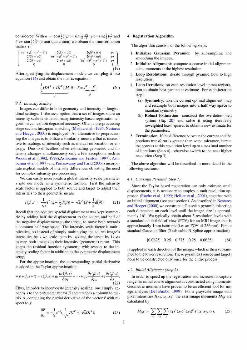
4.2. Initial Alignment (Step 2)

In order to speed up the registration and increase its capturerange, an initial coarse alignment is constructed using moments.Geometric moments have proven to be an efficient tool for im-age analysis (Del Bimbo, 1999). For a grayscale image withpixel intensities I(x1, x2, x3), the raw image moments Mi jk arecalculated by

Mi jk :=∑

x1

∑x2

∑x3

(x1)i (x2) j (x3)k I(x1, x2, x3), (25)

7

where i, j, k are the exponents of the coordinates x1, x2, x3 re-spectively (taking the values 0 or 1 in the following equation).The centroid of an image can be derived from the raw moments:

(x1, x2, x3)T :=(

M100

M000,

M010

M000,

M001

M000

)T

. (26)

We compute the translation needed to align the centroids anduse it by default as an initial transformation to ensure over-lapping images when starting the robust registration algorithm.Furthermore, it is possible to use central moments as definedbelow to compute an initial rotational alignment. For full headimages with possibly different cropping planes, such a rota-tional pre-alignment can be very inaccurate and should there-fore only be used when aligning skull stripped images. Centralmoments are defined translation invariant by using the centroid(Eq. 26):

µi jk :=∑

x1

∑x2

∑x3

(x1 − x1)i (x2 − x2) j (x3 − x3)k I(x1, x2, x3)

(27)The covariance matrix of the image I can now be defined usingµ′i jk := µi jk/µ000:

cov[I] =

µ′200 µ′110 µ′101µ′110 µ′020 µ′011µ′101 µ′011 µ′002

. (28)

The eigenvectors of the covariance matrix correspond to thethree principal axes of the image intensities (ordered accordingto the corresponding eigenvalues). These axes are then alignedfor two images. Care needs to be taken to keep the correct ori-entation. This is achieved by flipping the first eigenvector ifthe system has left-handed orientation. Even if both systemsare right-handed, it can still happen that two of the axes arepointing in the opposite direction, which can be detected andfixed by projecting each axis onto its corresponding axis in theother image and flipping it if necessary. If the angle betweenthe corresponding axes is too large, the correct orientation can-not be determined without additional information and the initialrotational alignment is not performed. Note that initial momentbased orientation alignment was never necessary and thereforenot used in any of our tests, since head MRI images are usuallyoriented similarly.

4.3. Loops (Step 3)There are three nested loops in the registration algorithm: the

different resolutions of the pyramid (step 3), several iterationson each level (remapping the images (step 4), and finally theiteratively reweighted least squares algorithm for the robust pa-rameter estimation (inside step 4(b), see Section 2.3). Note,when switching form a lower to a higher resolution in step 3,the translational parameters need to be adjusted (scaled by thefactor 2) when given in voxel coordinates.

4.4. Registration (Step 4)On each resolution level there are several iterations of the

resampling and robust parameter estimation as explained next.

4.4.1. Half Way Space (Step 4a)The registration model (Eq. 11) is designed to maintain sym-

metry in the algorithm, however we must also ensure that allsteps are performed similarly for both images. Therefore it isnot sufficient to map the source to the target in each iterationand re-estimate the new parameters. In such a setup only thesource would be resampled at (or close to) the target locationwhile the target would not go through the resampling process.In order to avoid this asymmetry, which can introduce biasesdue to the arbitrary specification of source and target, we pro-pose to resample both images to the half way space in eachiteration step.

For a given transformation T from the source to the target thehalf way maps are constructed by approximating the square rootof the matrix T (here T is again assumed to be a 4× 4 matrix inhomogeneous coordinates). For a positive definite matrix T (wedon’t allow reflections and projections) there exists exactly onepositive definite matrix T

12 with T = T

12 T

12 . For its computa-

tion we use the Denman-Beavers square root iteration (Denmanand Beavers, 1976; Cheng et al., 2001): Let Y0 = T and Z0 = I,where I is the identity matrix. The iteration is defined by

Yk+1 =12 (Yk + Z−1

k ),

Zk+1 =12 (Zk + Y−1

k ). (29)

The matrix Yk converges quadratically to the square root T12 ,

while Zk converges to its inverse, T−12 . Once T

12 has been ap-

proximated, the source image is mapped to T12 and the target

to T12 T−1 (to ensure both get resampled at the same location).

For the resampling process tri-linear interpolation is used, al-though other interpolation algorithms can easily be employed.Note that to maintain symmetry the square root iteration shouldonly be stopped when the largest element of abs(Y2

k −T ) is suf-ficiently small.

4.4.2. Robust Estimation (Step 4b)To set up the robust estimation problem (Eq. 20), the partial

derivatives and a smoothed version of both images need to becomputed. Smoothing is used to prevent the algorithm frombeing trapped in a local minimum. For smoothing we apply aGaussian kernel in each image direction (Nestares and Heeger,2000):

[0.03504 0.24878 0.43234 0.24878 0.03504] (30)

The smoothed derivatives can be computed by applying

[0.10689 0.28461 0.00000 0.28461 0.10689] (31)

in the direction of the derivative and the smoothing kernel inthe two other directions. Once the image derivatives DI arecomputed, the matrix A and vector ~b can be constructed (seeEq. 20). If the matrix gets too large, it is often sufficient tosubsample the image at the highest resolution and only selectevery second voxel. As the derivatives and intensity informa-tion are selected from the high resolutional image the result will

8

still be more accurate than stopping at the previous lower res-olution level in the Gaussian pyramid. For further improve-ment stochastic sampling algorithms can be employed to avoidaliasing. Subsampling specific regions more densely than oth-ers (e.g. depending on gradients, edges or the outlier weights) isalso likely to improve accuracy. Our tests, however, show veryaccurate results even with the simple subsampling algorithm.

Once the system has been constructed, the iterativelyreweighted least squares algorithm (Section 2.3) is employed tocompute the new parameters and weights. For this reason, thesaturation parameter c of the Tukey’s biweight functions mustbe specified. In Nestares and Heeger (2000) a constant satura-tion value c = 4.685 is recommended (suggested for Gaussiannoise in Holland and Welsch (1977)). However, a fixed valuecannot adjust well to different image contrast types and SNRlevels, such as non-linear deformations or larger intensity differ-ences. In these cases it can happen that the registration fails astoo many voxels are considered outliers. Therefore in order toreduce the number of detected outliers particularly in the brain,it is necessary to find a less sensitive (i.e. larger) value in thesecases. The user can always adjust this parameter according tothe specific image situation. For full head scans, however, wedeveloped a method that automatically estimates the sensitivityparameter. It also works remarkably well in brain-only regis-trations. For full head images, a global limit on the number ofoutlier voxels will not be a good measure, as large outlier re-gions especially at the skull, jaw and neck should be permitted.The following outlier measure uses a Gaussian to weigh vox-els at the center of the image more strongly than voxels furtheraway (see also Figure 5):

W :=∑

(1 − wi) e−d2i

2σ2∑e−

d2i

2σ2

, with σ =max(width,height,depth)

6

(32)where di is the distance of voxel i to the center. W is zero iff(if and only if) all weights wi are one (meaning no outliers). Alarge W means that many voxels in the center of the image arelabeled outlier. In that case the saturation is automatically in-cremented and W recomputed until W < Wthresh. All of this canbe computed quickly on a lower resolution level (we choosethe third highest level, i.e. for a 2563 image this is 643). Thethreshold Wthresh will be discussed and determined in Section5.4 Parameter Estimation. Note that in situations with signifi-cant outliers in the center, a global unweighted threshold can beused instead or the sensitivity parameter can be adjusted manu-ally.

4.5. Termination (Step 5)

In order to measure how much a new parameter estimate dif-fers from the last iteration, the root mean square (RMS) de-viation of the two corresponding transformations is computed.This measure will also be used to assess the quality of a reg-istration when compared to some ground truth. The RMS de-viation measures the average difference of voxel displacementsinside a spherical volume for two given affine transformations

Figure 5: Gaussian filter at the center(σ =

max(width,height,depth)6

).

(M1,~t1) and (M2,~t2), where M1,M2 are two 3 × 3 linear trans-formation matrices and t1, t2 the corresponding 3×1 translationvectors. The RMS error for a spherical volume with radius r isthen given by:

ERMS =

√15

r2 tr[(M2 − M1)T (M2 − M1)] + (~t2 − ~t1)T (~t2 − ~t1) ,

(33)where tr is the trace (see Jenkinson (1999) for the derivation).An average displacement error is used as a quality measure for atransformation instead of, for example, the maximum displace-ment because it depends on all voxels contained in the sphereinstead of possibly only a single voxel. The misalignment ofa single voxel is not very important if the rest of the image isaligned accurately. While a translation has an equally strong ef-fect everywhere, a rotation, for example, shifts voxels differentdistances depending on the distance to the rotation center. Fora translation of 0.1mm (and 1mm3 voxels) both maximum dis-placement and average displacement are the same ERMS = 0.1.Such a displacement can easily be seen on the screen whenswitching between the images. Even ERMS of 0.05 and belowcan be noticed when magnifying the images. These displace-ments, however, are too small to visualize in a printed versionof the image (e.g. checkerboard).

In this work the RMS error is measured on the transforma-tions defined in RAS (right, anterior, superior) coordinates withthe origin located approximately at the center of the image. Theradius of the spherical volume is set to r = 100 which corre-sponds to 100mm, enough to include the full brain. The iter-ations of the parameter estimation are usually terminated onceERMS < 0.01 i.e. the average displacement consecutive esti-mates are below 0.01mm, which is very restrictive. To avoidlong runtimes in ill conditioned cases, a maximum number ofiterations can also be specified by the user (the default is 5).

5. Results

This section presents results quantifying the accuracy and ro-bustness of the robust registration in comparison to other com-monly used methods. As mentioned above, the robust registra-tion is capable of ignoring outlier regions. This can be verifiedwhen checking the weights during a successful registration, as

9

Figure 6: The red/yellow regions (bottom row) are detected as outlier regionsduring the registraion procedure of this Multiecho MPRAGE test-retest data.Their influence is automatically reduced. It can be seen that the detected out-liers agree with the non-rigid differences after successful registration (top row)located mainly in the neck, eye, scalp and jaw/tongue region; see also Fig. 1.

shown in Figure 6. The top images show the (enhanced) dif-ferences between the target and registered source. The regionsthat contain the strongest differences are correctly detected asoutliers as can be seen in Figure 6 (bottom), where the weightsare overlayed (red/yellow regions). Note that the weights rangefrom 0 to 1 and are blurry (because they are computed onsmoothed images), so they can blur in from neighboring slices.

Figure 7 (left) is an example of an image that is misalignedusing FLIRT with the mutual information similarity function.The visible edges in the brain regions indicate an alignment er-ror. Figure 7 (right) shows the differences when using the robustregistration, where clearly less strong edges are visible. The re-maining residuals are due to resampling and noise. Figure 7bottom shows a magnification of the target (red) and registeredsource (green) on top of each other. The red and green edges(left) at the ventricle and temporal lobe indicate misalignmentwhile yellow regions are accurately aligned (right). The differ-ence between the two transforms here is ERMS = 0.88, almostone voxel on average.

In the following sections we analyze the performance of dif-ferent registration tools. We use the RMS deviation of twotransformations as described in Section 4.5 (Termination) toquantify the distance (the error) of a computed transformationwith respect to some ground truth transformation. For the fol-lowing tests we use a set of 14 healthy subjects each with twoscans 14 days apart. The images are MPRAGE T1 weightedfull head scans (on Siemens Sonata 1.5T) and are resampled to2563 voxels each with 1mm side length (original dimensions256 × 256 × 128 with 1mm ×1mm ×1.33mm voxels).

5.1. Inverse Consistency

Since this algorithm is intended to compute inverse consis-tent registrations, we need to verify experimentally that the fi-nal transforms are exactly inverses of each other when switch-ing source and target. For each subject we register the image

Figure 7: Difference after alignment. Left: FLIRT MI (the visible structures inthe brain indicate misalignment). Right: Robust method (accurate alignment,residual differences due to noise and resampling). The top shows the differ-ence images and the bottom a zoom-in into the aligned target (red) and source(green). A good alignment should be yellow (right) while the inaccurate regis-tration shows misaligned red and green edges (left).

head(orig) head−normalized(T1) brain−normalized(norm)0

0.02

0.04

0.06

0.08

0.1

0.12

RM

S E

rror

of T

rans

form

w.r

.t In

vers

e

Different Methods on 3 Image Types

Symmetry Comparison

FLIRT−LSFLIRT−CRFLIRT−MISPMLSRobustRobust−IRobust−I−SS

Figure 8: Comparison of inverse consistency using different methods: FLIRTLS: least squares , CR: correlation ratio, MI: mutual information, SPM, LS(our implementation with least squares instead of robust error function), Robustregistration, Robust-I (+intensity scaling) and Robust-I-SS (subsampling on thehighest resolution). The white circles represent the individual registrations.

10

Figure 9: Close-ups of test images: original (left) with Gaussian noise σ = 10(middle) and with outlier boxes (right).

from time point 2 to the time point 1 and vice versa while com-paring the obtained transforms of several common registrationalgorithms. We compare the robust registration (with differ-ent parameter settings) with the FLIRT registrations (Jenkinsonet al., 2002) from the FSL suite (Smith et al., 2004) using dif-ferent cost functions: standard least squares [FLIRT-LS], corre-lation ratio [FLIRT-CR], mutual information [FLIRT-MI]. Fur-thermore, we compare with a registration tool from the SPMsoftware (Ashburner and Friston, 1999) based on Collignonet al. (1995) [SPM]. The robust variants are: [Robust] robustrigid registration (no intensity scale), [Robust-I] with intensityscaling, and [Robust-I-SS] with additional subsampling at thehighest resolution. We also include our implementation withstandard least squares [LS] instead of the robust Tukey’s bi-weight error function to see the effect of the robust estimationwith no other differences in the algorithm. In Figure 8 the RMSdeviation of the forward and inverse backward transforms arecomputed and compared for different image types as used in theFreeSurfer software package: full head scans (orig), intensitynormalized images (T1) and normalized skull stripped images(norm).

The FLIRT registrations perform similarly. The higher meanin the mutual information method on the orig images is due toa single outlier (ERMS = 2.75). It can be seen that the robustregistration methods are extremely symmetric, even with inten-sity scaling switched on, adding another degree of freedom anda higher chance for numerical instabilities. Also our non-robustmethod [LS] with the standard least squares error function isperfectly symmetric in all cases. This test, however, does nottell us anything about the accuracy of the registration.

5.2. Tests Using Synthetic Data

In this section we present results using images that weretransformed, intensity scaled and otherwise manipulated withknown transformations, which then can be used as ground truth.We compare how well several registration algorithms performon the same test set of the 14 MPRAGE T1 weighted full headscans (Siemens Sonata 1.5T) of the same healthy subjects. Theregistration methods are the same as in the previous section(FLIRT, SPM and robust registration).

A random rigid transformation (rotation, translation) wascomputed for each image. The parameters were chosen in away that reflects possible (large) head movements in a scanner:50mm translation in a random direction together with a random

rotation of 25◦ around an arbitrary axis with the origin at thecenter of the image. The maximum displacement of a corner oftheses image was between 130mm and 140mm. The parame-ters were chosen, so that all methods can find approximate solu-tions. For larger transformations [SPM] was no longer capableof recovering the correct registrations at all, while the robustmethods performed perfectly (not shown) in tests up to 100mmtranslation and 40◦ rotation. These transformations move theimages apart so that there is almost no overlap, furthermoreparts of the face, skull, neck and jaw can be cropped becausethey are mapped outside the field-of-view. The robust approachcan deal well with this kind of partial matching. Moreover, webelieve that, due to the multiresolution algorithm and the initialmoment based alignment, even larger transformations will berecovered accurately.

For the synthetic registration comparison, the transform thatrepresents half the random translation and rotation is used tomap and resample each image at the target location and the in-verse is applied to map and resample each image at the sourcelocation. This ensures that both images (source and target) willbe resampled and do not move outside the field of view as eas-ily. An accurate registration from source to target needs to beclose to the original random transform. The accuracy is mea-sured using the RMS deviation (see Section 4.5) of the groundtruth and the computed transformation matrix. Four differenttests were performed. In all cases random rigid motion wasapplied (as described above):

1. Only-Motion: only random rigid motion.2. Noise: significant Gaussian noise was added with σ = 10

(Figure 9 middle).3. Outlier boxes: 80 boxes (each box 303 voxel) were created

and copied from a random location to another random lo-cation within the same image, with 40 boxes each in sourceand target (Figure 9 right).

4. Intensity: global intensity scaling (±5%) was performed.

The results of this experiment are given in Figure 10. It canbe seen that the robust version outperforms the three differentFLIRT similarity functions in all tests. [SPM] yields similar ac-curacy, but fails completely for larger transforms (not shown).The robust registration shows almost no influence of the out-lier boxes since these are accurately detected as such. There isonly little influence of noise. However, when the global inten-sity scale is different in the two images, the robust registrationmethods needs 7 DOF (one additional intensity scale parameter:[Robust-I]) to maintain accuracy, because it strongly dependson similar intensity levels. This underlines the importance ofincorporating automatic intensity scaling into the robust regis-tration method. Subsampling on the highest resolution in the ro-bust registration [Robust-I-SS] leads to a significant reductionin memory and run time, but still yields the same registrationaccuracy in these tests. The simple non-robust implementationLS performs poorly in most cases.

It should be noted that the FLIRT methods produce a few in-dividual registrations with low accuracy when outliers or noiseare present (as can be seen by checking the scatter data, thesmall circles in Figure 10, some are too large and not shown).

11

only−motion noise(10) outlier−boxes(80) intensity0

0.02

0.04

0.06

0.08

0.1

0.12

0.14

RM

S E

rror

of T

rans

form

(to

Gro

und

Tru

th)

Different Test With Random Motion Plus Additional Obstacles

Simulated Motion Comparison

FLIRT−LSFLIRT−CRFLIRT−MISPMLSRobustRobust−IRobust−I−SS

Figure 10: Accuracy of different methods (see Fig.8). The four different testsare: random rigid motion, additional Gaussian noise (σ = 10mm), 80 boxes ofoutlier data and intensity scaling.

The SPM method on the other hand produces quite accurate re-sults in most test cases. However, as mentioned above it failscompletely for larger transformations.

5.3. Tests Using Real Data

In contrast to the simulations with available ground truthtransformations we do not know the correct registration in ad-vance in typical registration paradigms. Therefore we need toestablish a different performance metric. This can be achievedby registering the skull stripped and intensity normalized im-ages of a test-retest study (two time points) with different regis-tration methods. These registrations are highly accurate as theimages contain only brains of healthy normals and only smallchanges in the brain are involved (e.g. noise etc.). In these wellbehaved situations the registration of these brain images com-puted by the different algorithms deviate from each other onlyby small amounts. The goal here is to find registrations of thecorresponding full head images that are as close as possible tothe brain-only, intensity normalized registrations.

The group chosen for this test is the same as described above.This test will be more noisy as the ’ground truth’ is already de-fined inaccurately. Figure 11 (left) shows the distances of allother methods to the SPM registration of the skull stripped nor-malized image (norm). It can be seen that compared to the fullhead registrations, the norm registrations are on a similar lowlevel for all methods (SPM has of course zero distance to itself).SPM has been chosen to construct the ground truth registra-tion of the norm images, as it performed more accurately thanthe FLIRT methods in the previous tests. We did not choosea robust registration to establish the ground truth to not favorour method. However, we tested establishing the ’ground truth’with any other method which leads to very similar results andalmost exactly the same plots.

brain−normmalized(norm) head(orig) head−normalized(T1)0

0.1

0.2

0.3

0.4

0.5

0.6

0.7

RM

S E

rror

of T

rans

form

(w

.r.t.

SP

M o

n no

rm)

Different Methods on 3 Image Types

Accuracy of Registration TP2 to TP1

FLIRT−LSFLIRT−CRFLIRT−MISPMLSRobustRobust−IRobust−I−SS

Figure 11: Accuracy of different methods (see Fig.8) with respect to SPM (onthe norm images).

The results on the full head (orig) image (Figure 11 middle)and intensity normalized full head (T1) image (Figure 11 right)evidence behavior that is similar to the previous tests. SPM per-forms (here only slightly) better than the FLIRT methods, whilethe robust registration yields the most accurate results. As ex-pected for the orig images intensity scaling [Robust-I] improvesthe registrations further, while for the normalized T1 images itis not necessary. Again subsampling [Robust-I-SS] on the high-est resolution reaches the same accuracy, indicating that the ex-pensive iterations on the highest resolution level can be avoided.

5.4. Parameter Estimation

As described in Section 4.4.2 a fixed saturation level c cannotbe recommended for all image types. The value c = 4.685 fromNestares and Heeger (2000) will lead to erroneous registrationsin many common settings. Figure 12 (top) shows the accuracyof each robust registration of the orig images plotted vs. the se-lected saturation level. For some subjects the optimal registra-tion is reached at c ≈ 6 while other need a higher value c ≈ 15.For the normalized T1 images or for [Robust-I] (with intensityscaling enabled) the results look similar (not shown), howeverwith individual minima spread between c = 4 and c = 9. Whenusing a fixed saturation level for all registrations, c ≈ 14 is op-timal for [Robust] with an average RMS error of slightly below0.3 and c = 8.5 is optimal for [Robust-I]. Even with a fixedsaturation, both robust methods are on average better than theother non-robust registration methods (cf. Figure 12 bottom).

For [Robust] without intensity scaling, a relative high satu-ration value (c = 14) is particularly necessary to compensatefor the differences in image intensity. Lower values might la-bel too many voxels outlier due to the intensity differences ornon-linearities, resulting in misaligned images (see Figure 13for an example). Instead of manually inspecting the outliersand registrations while determining an optimal saturation set-

12

4 6 8 10 12 14 16 18 20 220

0.2

0.4

0.6

0.8

1

1.2

1.4

1.6

1.8

RM

S E

rror

of T

rans

form

(w

.r.t.

SP

M o

n no

rm)

Fixed Saturation Levels

Accuracy vs. Saturation, Scatter, [Robust]

4 6 8 10 12 14 16 18 20 220.2

0.25

0.3

0.35

0.4

0.45

0.5

0.55

0.6

0.65

RM

S E

rror

of T

rans

form

(w

.r.t.

SP

M o

n no

rm)

Fixed Saturation Levels

Accuracy vs. Saturation, Averages

FLIRT−LSFLIRT−CRFLIRT−MISPMRobustRobust−I

Figure 12: Top: Accuracy of [Robust] for each individual subject. Bottom:Mean accuracy of the methods, where [Robust] and [Robust-I] depend on thesaturation level (fixed across all subjects). It can be seen (bottom) that [Robust]reaches its minimal average registration error at the fixed saturation level ofc = 14 and [Robust-I] at c = 8.5. For most fixed saturation levels, both methodsperform better on average than FLIRT or SPM (note, the averages of [FLIRT-LS] and [FLIRT-CR] almost coincide, compare with Fig. 11 middle).

Figure 13: Top: Fixed low saturation of c = 4.685 (high outlier sensitivity) ina registration with intensity differences and non-linearities results in too manyoutlier and consequently in misalignment. Bottom: Automatic sensitivity esti-mation adjusts to a higher saturation value (low outlier sensitivity) to registerthe images successfully. The detected outlier regions are labeled red/yellow.

0 0.1 0.2 0.3 0.4 0.5 0.60

0.2

0.4

0.6

0.8

1

1.2

1.4

1.6

RM

S E

rror

of T

rans

form

(w

.r.t.

SP

M o

n no

rm)

Center Focused Outlier Measure W

Accuracy vs. Outlier Measure W [Robust]

Average at WAverage of Optimal Registrations

0 0.1 0.2 0.3 0.4 0.5 0.60

0.2

0.4

0.6

0.8

1

1.2

1.4

1.6

RM

S E

rror

of T

rans

form

(w

.r.t.

SP

M o

n no

rm)

Center Focused Outlier Measure W

Accuracy vs. Outlier Measure W [Robust−I]

Average at WAverage of Optimal Registrations

Figure 14: Registration accuracy for each subject depending on center fo-cused weight W (Robust top, Robust-I bottom). Red horizontal line: averagingbest registration per subject. Black curve: average performance at specific W.Dashed curves: individual subject’s results.

ting per image, we introduce the center focused weight mea-sure W (Eq. 32) for full head images to indicate when too manyoutliers are detected in brain regions and to adjust the sensitiv-ity accordingly. Figure 13 (bottom row) shows the same imageregistration, where the automatic parameter estimation resultsin less detected outliers and a successful alignment.

We will now determine an optimal W for the automatic sat-uration estimation. Figure 14 presents scatter plots of registra-tion accuracies [Robust] and [Robust-I] on the full head (orig)images here plotted versus W. The horizontal red line showsthe average minimum error when choosing the individual satu-ration that leads to the best registration for each subject (withrespect to the ground truth). The automatic saturation estima-tion can almost reach this optimum by fixing the center focusedweight measure W around 0.2 (see the black curve showing theaverage of W between 0.05 and 0.3). Additionally, W is quiterobust since the average (black dashed curve) is relatively flat.Ensuring a W around 0.2 for the tested image types in the auto-matic saturation estimation leads to registrations that are almostas accurate as when taking the optimal result per subject (whichis of course not know a priori).

13

FLIRT−LS FLIRT−CR FLIRT−MI SPM LS Robust Robust−IRobust−I−SS

0

2

4

6

8

10

12

14

16

18

20x 10

6

SS

E S

igne

d D

iffer

ence

to R

obus

t−I

Different Registration Algorithms

SSE Comparison (within Brain Mask)

FLIRT−LSFLIRT−CRFLIRT−MI SPM LS Robust Robust−IRobust−I−SS−200

0

200

400

600

800

1000

1200

1400

Num

ber

of E

dges

Sig

ned

Diff

eren

ce to

Rob

ust−

I

Different Registration Algorithms

Avg. Image: Edge Count within Brain Mask

Figure 15: Error of motion correction task in brain region for different registration methods Left: sum of squared errors comparison. Right: edge count of averageimage. Both plots show the signed difference to Robust-I.

5.5. Application: Motion CorrectionFrequently several images of a given scan type are acquired

within a session and averaged in order to increase SNR. Theseimages are not perfectly aligned due to small head movementsin the scanner (for some groups of patients there can be evenlarge differences in head location, due to uncontrolled motion)and need to be registered first. Since not only noise but otherdifferences such as jaw movement or motion artifacts are preva-lent in these images, a robust registration method should be op-timally suited to align the images while discounting these out-lier regions. It can be expected that except for noise, brain tissueand other rigid parts of the head will not contain any significantdifferences (except rigid location changes). A misalignment ofthe within-session scans will of course affect the average imagenegatively and can reduce the accuracy of results generated bydownstream processes. Therefore highly accurate registrationsfor motion correction are the first step, for example, towards de-tecting subtle morphometric differences associated with diseaseprocesses or therapeutic intervention.

To test the robust registration for this type of within-sessionmotion correction, the two scans of the first session in the longi-tudinal data set presented above were selected. The second scanwas registered to the first with the different registration meth-ods. It was then resampled at the target location (first scan)and an average image was created. Since these within-sessionscans should show no change in brain anatomy, it can be ex-pected that the difference between scan 1 and aligned scan 2 inbrain regions will be very small and mainly be due to noise (andof course scan 2 will be smoother due to resampling). There-fore a larger difference in the brain-region between the regis-tered images implies misalignment, most likely due to imagedifferences elsewhere (e.g. jaw, neck and eyes) or less likely dueto non-linear differences between the two scans. The gradientnon-linearities will badly influence all rigid registrations sim-ilarly, while possible non-brain outlier regions will influencethe employed methods differently. Therefore we will evaluate

the performance of full head registration only within the brainmask.2

We first quantify the registration error and compute the sumof squared errors (SSE) of the intensity values in scan I1 andaligned/resampled scan I2:

S S E =∑i∈B

(I1(i) − I2(i))2 (34)

where the sum is taken over all brain voxels B. The brain masksto specify brain regions were created automatically for eachsubject with the FreeSufer software package and visually in-spected to ensure accuracy.

The SSE measure quantifies the intensity differences of thetwo images after alignment within the brain. For a perfect re-gistration these differences should be small as they only mea-sure noise, non-linearities and global intensity scaling (all ofthese should be small as the two images are from the samescan session). Figure 15 (left) shows the signed difference ofSSE with respect to the result of the method [Robust-I]. Therobust methods perform best on average, while [FLIRT-LS],[FLIRT-CR] and [LS] yield a better results (lower SSE) only inone single instance (white circles with negative value). To testthe significance of these results, we applied a Wilcoxon signedrank test (Wilcoxon , 1945) for each algorithm with respect to[Robust-I] to test if the median of the pairwise differences isequal to zero (null hypothesis). This is similar to the t-test onthe pairwise differences, without the assumption of normally

2In some applications it might be better to compute registrations on skullstripped brains directly. However automatic skull stripping is a complex proce-dure, and frequently needs the user to verify all slices manually. Furthermore,in some situations it makes sense to keep the skull, for example, when regis-tering to a Talairach space with skull to estimate intracranial content, whichdepends on head size rather than brain size. Finally even skull stripped imagescan contain significant differences, for example in longitudinal data or simplybecause different bits of non-brain are included, so that the robust registrationis still the best choice.

14

distributed data. We found that all non-robust methods showsignificant differences from [Robust-I] at a p < 0.001 while thenull hypothesis cannot be rejected within the robust methods,as expected, since their performance is basically the same.

In order to test if differences can be detected in the result-ing average images, we count the number of edges. Correctlyaligned images should minimize the number of edges since alledges will be aligned, while misalignment increases the edgecount. The edges were detected by scanning the x componentof the gradient (using the Sobel filter) in the x directions andcounting local maxima above a threshold of 5. Figure 15 (right)shows that the misalignment increases edge count on averagewhen compared to [Robust-I]. However, due to the large vari-ance the FLIRT results are not significant. [SPM] is signifi-cantly different at level p = 0.058 and [LS] at the p < 0.001significance level in the Wilcoxon signed rank test.

6. Conclusion

In this work a robust registration method based on Nestaresand Heeger (2000) is presented, with additional properties suchas initial coarse alignment, inverse consistency, sensitivity pa-rameter estimation and global intensity scaling. Automatic in-tensity scaling is necessary for the method to function whenglobal intensity differences exist. Similarly the automatic esti-mation of the saturation parameter avoids misalignment in spe-cific image situations where a fixed value potentially ignorestoo many voxels.

The presented method outperforms commonly used state-of-the-art registration tools in several tests, and produces resultsthat are optimally suited for motion correction or longitudinalstudies, where images are taken at different points in time. Lo-cal differences in these images can be very large due to move-ment or true anatomical change. These differences will in-fluence the registration result, if a statistically non-robust ap-proach is employed. In contrast, the robust approach presentedhere maintains high accuracy and robustness in the presence ofnoise, outlier regions and intensity differences.

The symmetric registration model together with the ’halfway’ space resampling ensure inverse consistency. If an un-biased average of two images is needed, it is easily possibleto resample both, target and source, at the ’half way’ loca-tion and perform the averaging in this coordinate system. Fur-thermore, these registrations can be employed to initialize non-linear warps without introducing a bias. Robust registration hasbeen successfully applied in several registration tasks in our lab,including longitudinal processing and motion correction. Thesoftware is freely available within the FreeSurfer package asthe mri robust register tool.

Future research will extend the presented registration to morethan two images and incorporate these algorithms into a lon-gitudinal processing stream, where more than two time pointsmay be involved. In those settings instead of simply register-ing all images to the first time point, it is of interest to createan unbiased template image and simultaneously align all inputimages in order to transfer information at a specific spatial loca-tion across time. Similar to the idea in (Avants and Gee, 2004) it

is possible to estimate the unbiased (intrinsic) mean image andthe corresponding transforms iteratively based on the pairwiseregistration algorithm described in this paper.

7. Acknowledgements

Support for this research was provided in part by the NationalCenter for Research Resources (P41 RR14075, and the NCRRBIRN Morphometric Project BIRN002, U24 RR021382),the National Institute for Biomedical Imaging and Bioengi-neering (R01 EB006758), the National Institute on Ag-ing (R01 AG022381,U54 AG024904), the National Insti-tute for Neurological Disorders and Stroke (R01 NS052585,R01 NS042861, P01 NS058793). Additional support was pro-vided by The Autism & Dyslexia Project funded by the EllisonMedical Foundation. The authors would like to thank Dr. GregSorensen for kindly supplying the tumor sample data.

References

Ashburner, J., Friston, K., 1997. Multimodal image coregistration and parti-tioning – a unified framework. NeuroImage 6 (3), 209 – 217.

Ashburner, J., Friston, K., 1999. Nonlinear spatial normalization using basisfunctions. Human Brain Mapping 7 (4), 254–266.

Ashburner, J., Neelin, P., Collins, D. L., Evans, A., Friston, K., 1997. Incor-porating prior knowledge into image registration. NeuroImage 6 (4), 344 –352.

Avants, B., Gee, J.C., 2004. Geodesic estimation for large deformation anatom-ical shape averaging and interpolation. NeuroImage 23 (1), 139–150.

Bajcsy, R., Kovavcivc, S., 1989. Multiresolution elastic matching. ComputerVision Graphics and Image Processing 46 (1), 1–21.

Beg, M.F., Kahn, A., 2007. Symmetric Data Attachment Terms for LargeDeformation Image Registration. IEEE Transactions on Medical Imaging26 (9), 1179–1189.

Bican, J., Flusser, J., 2009. 3D Rigid registration by cylindrical phase correla-tion method. Pattern Recognition Letters 30, 914–921.

Bookstein, F. L., 1989. Principal warps: Thin-plate splines and the decompo-sition of deformations. IEEE Transactions on Pattern Analysis and MachineIntelligence 11, 567–585.

Bookstein, F. L., 1991. Thin-plate splines and the atlas problem for biomedicalimages. In: IPMI ’91: Proceedings of the 12th International Conference onInformation Processing in Medical Imaging. Springer-Verlag, pp. 326–342.

Cheng, S. H., Higham, N. J., Kenney, C. S., Laub, A. J., 2001. Approximatingthe logarithm of a matrix to specified accuracy. SIAM Journal on MatrixAnalysis and Applications 22 (4), 1112–1125.

Christensen, G. E., Rabbitt, R. D., Miller, M. I., 1994. 3D brain mapping usinga deformable neuroanatomy. Physics in Medicine and Biology 39 (3), 609–618.

Christensen, G. E., Johnson, H. J., 2001. Consistent Image Registration. IEEETransactions on Medical Imaging 20 (7),568–582.

Collignon, A., Maes, F., Delaere, D., Vandermeulen, D., Suetens, P., Marchal,G., 1995. Automated multi-modality image registration based on informa-tion theory. In: Information Processing in Medical Imaging. Kluwer, pp.263–274.

Collins, D., Holmes, C., Peters, T., Evans, A., 1995. Automatic 3-D model-based neuroanatomical segmentation. Human Brain Mapping 3 (3), 190–208.

Costagli, M., Waggoner, R.A., Ueno, K., Tanaka, K., Cheng, K., 2009. Correc-tion of 3D rigid body motion in fMRI time series by independent estimationof rotational and translational effects in k-space. NeuroImage 45, 749–757.

Dale, A. M., Fischl, B., Sereno, M. I., 1999. Cortical surface-based analysis: I.segmentation and surface reconstruction. NeuroImage 9 (2), 179 – 194.

Del Bimbo, A., 1999. Visual information retrieval. Morgan Kaufmann Publish-ers Inc. San Francisco.

Denman, E. D., Beavers, A. N., 1976. The matrix sign function and computa-tions in systems. Applied Mathematics and Computation 2 (1), 63–94.

15

Dickerson, B., Goncharova, I., Sullivan, M., Forchetti, C., Wilson, R., Bennett,D. A., Beckett, L., deToledo Morrell, L., 2001. MRI-derived entorhinal andhippocampal atrophy in incipient and very mild alzheimer’s disease. Neuro-biological Aging 22, 747–754.

Evans, A., Marrett, S., Collins, D., Peters, T., 1989. Anatomical-functional cor-relative analysis of the human brain using three-dimensional imaging sys-tems. In: Proceedings of the SPIE - The International Society for OpticalEngineering. Vol. 1092. pp. 264–274.

Fischl, B., Sereno, M. I., Dale, A. M., 1999. Cortical surface-based analysis:Ii: Inflation, flattening, and a surface-based coordinate system. NeuroImage9 (2), 195 – 207.

Frackowiak, R., Friston, K., Frith, C., Dolan, R., Price, C., Zeki, S., Ashburner,J., Penny, W., 2003. Human Brain Function, 2nd Edition. Academic Press.

Gee, J. C., Gee, J. C., Reivich, M., Reivich, M., Bajcsy, R., Bajcsy, R., 1993.Elastically deforming a three-dimensional atlas to match anatomical brainimages. Computer Assisted Tomography 17 (2), 225–236.

Greve, D. N., Fischl, B., 2009. Accurate and robust brain image alignment usingboundary-based registration. NeuroImage 48 (1), 63 – 72.

Hellier, P., Barillot, C., Memin, E., Perez, P., 2001. Hierarchical estimation ofa dense deformation field for 3-D robust registration. IEEE Transactions onMedical Imaging 20 (5), 388–402.

Hill, D. L. G., Batchelor, P. G., Holden, M., Hawkes, D. J., 2001. Medicalimage registration. Physics in Medicine and Biology 46 (3), R1–R45.

Holland, P. W., Welsch, R. E., 1977. Robust regression using iterativelyreweighted least-squares. Communications in Statistics - Theory and Meth-ods 6 (9), 813–827.

Huber, P. J., 1964. Robust estimation of a location parameter. Annals Math.Statist. 35, 73–1001.

Jack, C. R., Petersen, R. C., Xu, Y. C., Waring, S. C., O’Brien, P. C., Tangalos,E. G., Smith, G. E., Ivnik, R. J., Kokmen, E., 1997. Medial temporal atrophyon mri in normal aging and very mild alzheimer’s disease. Neurology 49 (3),786–790.

Jenkinson, M., 1999. Measuring transformation error by RMS deviation. Tech.Rep. TR99MJ1, Oxford Center for Functional Magnetic Resonance Imagingof the Brain (FMRIB).

Jenkinson, M., Bannister, P. R., Brady, J. M., Smith, S. M., 2002. Improvedoptimization for the robust and accurate linear registration and motion cor-rection of brain images. NeuroImage 17, 825–841.

Kerwin, W., Yuan, C., 2001. Active edge maps for medical image registration.In: Medical Imaging 2001: Image Processing. Vol. 4322. SPIE, pp. 516–526.

Kochunov, P., Lancaster, J. L., Glahn, D. C., Purdy, D., Laird, A. R., Gao, F.,Fox, P., 2006. Retrospective motion correction protocol for high-resolutionanatomical mri. Human Brain Mapping 27 (12), 957–962.

Kostelec, P., Weaver, J., Healy, D. J., 1998. Multiresolution elastic image regis-tration. Medical Physics 25 (9), 1593–1604.

van der Kouwe, A., Benner, T., Dale, A., 2006. Real-time rigid body motioncorrection and shimming using cloverleaf navigators. Magnetic Resonancein Medicine 56 (5), 1019–1032.

Kuperberg, G. R., Broome, M., McGuire, P. K., David, A. S., Eddy, M., Ozawa,F., Goff, D., West, W. C., Williams, S., van der Kouwe, A., Salat, D., Dale,A. M., Fischl, B., 2003. Regionally localized thinning of the cerebral cortexin Schizophrenia. Archives of General Psychiatry 60, 878–888.

Kybic, J., Thevenaz, P., Nirkko, A., Unser, M., 2000. Unwarping of unidi-rectionally distorted EPI images. IEEE Transactions on Medical Imaging19 (2), 80 – 93.

Lerch, J. P., Pruessner, J. C., Zijdenbos, A., Hampel, H., Teipel, S. J., Evans,A. C., 2005. Focal decline of cortical thickness in Alzheimer’s disease iden-tified by computational neuroanatomy. Cerebral Cortex 15, 955–1001.

Maes, F., Collignon, A., Vandermeulen, D., Marchal, G., Suetens, P., 1997.Multimodality image registration by maximization of mutual information.IEEE Transactions on Medical Imaging 16 (2), 187–198.

Maes, F., Vandermeulen, D., Suetens, P., 1999. Comparative evaluation of mul-tiresolution optimization strategies for multimodality image registration bymaximization of mutual information. Medical Image Analysis 3, 373–386.

Maintz, J., Viergever, M., 1998. A survey of medical image registration. Medi-cal Image Analysis 2 (1), 1–36.

Medioni, G., Nevatia, R., 1984. Matching images using linear features. PatternAnalysis and Machine Intelligence 6 (6), 675–685.

Mishra, D., Chan, A. K., Chui, C. K., 1995. Histogram equalization, imageregistration, and data fusion for multispectral images. In: Proceedings of

the SPIE - The International Society for Optical Engineering. Vol. 2496. pp.1025–1031.

Nack, M., 1977. Rectification and registration of digital images and the effect ofcloud detection. In: Proceedings of Machine Processing of Remotely SensedData. pp. 12–23.

Narr, K. L., Bilder, R. M., Toga, A. W., Woods, R. P., E., R. D., Szeszko, P. R.,Robinson, D., Sevy, S., Gunduz-Bruce, H., Wang, Y.-P., Deluca, H., Thomp-son, P., 2005. Mapping cortical thickness and gray matter concentration infirst episode Schizophrenia. Cerebral Cortex 15, 708–719.

Nestares, O., Heeger, D. J., 2000. Robust multiresolution alignment of MRIbrain volumes. Magnetic Resonance in Medicine 43 (5), 705–715.

Pelizzari, C. A., Chen, G. T. Y., Spelbring, D. R., Weichselbaum, R. R., Chen,C.-T., 1989. Accurate three-dimensional registration of CT, PET, and/or MRimages of the brain. Journal of Computer Assisted Tomography 13 (1), 20–26.

Periaswamy, S., Farid, H., 2006. Medical image registration with partial data.Medical Image Analysis 10 (3), 452 – 464, Special Issue on The SecondInternational Workshop on Biomedical Image Registration (WBIR’03).

Roche, A., Malandain, G., Ayache, N., Prima, S., 1999. Towards a bettercomprehension of similarity measures used in medical image registration.In: MICCAI ’99: Proceedings of the Second International Conference onMedical Image Computing and Computer-Assisted Intervention. Vol. 1679.Springer-Verlag, pp. 555–566.

Roche, A., Malandain, G., Pennec, X., Ayache, N., 1998. The correlation ratioas a new similarity measure for multimodal image registration. In: Proceed-ings MICCAI’98. Vol. 1496 of LNCS. Springer Verlag, pp. 1115–1124.

Rosas, H. D., Liu, A. K., Hersch, S., Glessner, M., Ferrante, R. J., Salat, D.,van der Kouwe, A., Jenkins, B. G., Dale, A. M., Fischl, B., 2002. Regionaland progressive thinning of the cortical ribbon in Huntington’s disease. Neu-rology 5 (5), 695–701.

Rueckert, D., Sonoda, L., Hayes, I., Hill, D. L. G., Leach, M., Hawkes, D. J.,1999. Nonrigid registration using free-form deformations: Application tobreast MR images. IEEE Transactions on Medical Imaging 18 (8), 400–721.

Saad, Z. S., Glen, D. R., Chen, G., Beauchamp, M. S., Desai, R., Cox, R. W.,2009. A new method for improving functional-to-structural mri alignmentusing local pearson correlation. NeuroImage 44 (3), 839 – 848.

Sailer, M., Fischl, B., Salat, D., Tempelmann, C., Schonfeld, M., Busa, E., Bo-dammer, N., Heinze, H.-J., Dale, A. M., 2003. Focal thinning of the cerebralcortex in multiple sclerosis. Brain 126 (8), 1734–1744.

Salat, D., Buckner, R., Snyder, A., Greve, D. N., Desikan, R., Busa, E., Morris,J., Dale, A. M., Fischl, B., 2004. Thinning of the cerebral cortex in aging.Cerebral Cortex 14, 721–730.

Salat, D., Kaye, J., Janowsky, J., 1999. Prefrontal gray and white matter vol-umes in healthy aging and alzheimer disease. Archives of Neurology 56 (3),338–44.

Schonemann, P., 1931. A generalized solution of the orthogonal procrustesproblem. Psychometrika 31 (1), 1–10.

Shih, W., Lin, W., Chen, C., 1997. Contour-model-guided nonlinear deforma-tion model for intersubject image registration. In: Proceedings of the SPIE -The International Society for Optical Engineering. Vol. 3034. pp. 611–620.

Smith, S. M., Jenkinson, M., Woolrich, M. W., Beckmann, C. F., Behrens, T. E.,Johansen-Berg, H., Bannister, P. R., De Luca, M., Drobnjak, I., Flitney,D. E., Niazy, R. K., Saunders, J., Vickers, J., Zhang, Y., De Stefano, N.,Brady, J. M., Matthews, P. M., 2004. Advances in functional and structuralMR image analysis and implementation as FSL. NeuroImage 23, 208–219.

Sowell, E. R., Peterson, B. S., Thompson, P., Welcome, S. E., Henkenius, A. L.,Toga, A. W., 2003. Mapping cortical changes across the human life span.Nature Neuroscience 6, 309–315.

Sowell, E. R., Thompson, P., Leonard, C. M., Welcome, S. E., Kan, E., Toga,A. W., 2004. Longitudinal mapping of cortical thickness and brain growthin normal children. J Neuroscience 24 (38), 8223–8231.

Stewart, C. V., 1999. Robust parameter estimation in computer vision. SIAMReviews 41, 513–537.

Thompson, P., Hayashi, K. M., Zubicaray, G., Janke, A. L., Rose, S. E., Semple,J., Herman, D., Hong, M. S., Dittmer, S., Doddrell, D. M., Toga, A. W.,2003. Dynamics of gray matter loss in alzheimer’s disease. J Neuroscience23 (3), 994–1005.

Thompson, P., Vidal, C. N., Giedd, J., Gochman, P., Blumenthal, J., Nicol-son, R., Toga, A. W., Rapoport, J., 2001. Mapping adolescent brain changereveals dynamic wave of accelerated gray matter loss in very early onsetSchizophrenia. Proceedings of National Academy of Sciences USA 98 (20),

16

11650–11655.Unser, M., Aldroubi, A., Gerfen, C., 1993. A multiresolution image registration

procedure using spline pyramids. In: Proceedings of the SPIE Conferenceon Mathematical Imaging: Wavelet Applications in Signal and Image Pro-cessing. Vol. 2034. pp. 160–170.

Wells, W., Viola, P., Atsumi, H., Nakajima, S., Kikinis, R., 1996. Multi-modalvolume registration by maximization of mutual information.

West, J., Fitzpatrick, J. M., Wang, M. Y., Dawant, B. M., Maurer, C. J., Kessler,R. M., Maciunas, R. J., 1999. Retrospective intermodality registration tech-niques for images of the head: surface-based versus volume-based. IEEETransactions on Medical Imaging 18 (2), 144–150.

West, J., Fitzpatrick, J. M., Wang, M. Y., Dawant, B. M., Maurer, C. R., Kessler,R. M., Maciunas, R. J., Barillot, C., Lemoine, D., Collignon, A., Maes, F.,Sumanaweera, T. S., Harkhess, B., Hemler, P. F., Hill, D. L. G., Hawkes,D. J., Studholme, C., Maintz, J. B. A., Viergever, M. A., Mal, G., Pennec,X., Noz, M. E., Maguire, G. Q., Pollack, M., Pelizzari, C. A., Robb, R. A.,Hanson, D., Woods, R. P., 1997. Comparison and evaluation of retrospec-tive intermodality brain image registration techniques. Journal of ComputerAssisted Tomography 21 (4), 554–566.

Wilcoxon, F., 1945. Individual comparisons by ranking methods. Biometrics 1,80–83.

Woods, R. P., Cherry, S., Mazziotta, J., 1992. Rapid automated algorithm foraligning and reslicing PET images. Computer Assisted Tomography 16 (4),620–633.

Woods, R. P., Grafton, S., Holmes, C., Cherry, S., Mazziotta, J., 1998. Auto-mated image registration: I. general methods and intrasubject, intramodalityvalidation. Computer Assisted Tomography 22 (1), 139–152.

Yeung, S.K., Tang, C.K., Shi, P.C., Pluim, J.P.W., Viergever, M.A., Chung,A.C.S., Shen, H.C., 2008. Enforcing stochastic inverse consistency in non-rigid image registration and matching. In Proceedings CVPR’08, 8 pages.

Yushkevicha, P. A., Avantsa, B. B., Dasa, S. R., Plutab, J., Altinaya,M., Craigea, C., 2009. Bias in estimation of hippocampal atrophy usingdeformation-based morphometry arises from asymmetric global normaliza-tion: An illustration in ADNI 3 tesla MRI data. NeuroImage 50 (2), 434-445.

Zeng, Q., Chen, Y.,2008. Accurate Inverse Consistent Non-rigid Image Regis-tration and Its Application on Automatic Re-contouring. In BioinformaticsResearch and Applications, ISBRA’08, 293–304, Lecture Notes in Com-puter Science 4983, Springer.

17