Highlights of Chapter 12 2 Scientific truth always goes through three stages. First, people say it conflicts with the Bible; next they say it has been.

Highlights of Chapter 12

2

Scientific truth always goes through three stages. First, people say it conflicts with the Bible; next they say it has been discovered before; and lastly they say that they always believed it

Louis Agassiz, Swiss naturalist

We do not now a truth without knowing its cause

Aristotle, Nicomachean Ethics

Development of Western science is based on two great achievements: the invention of the formal logical system (Euclidean geometry) by the Greek philosophers, and the discovery of the possibility to find out causal relationships by systematic experiment (during the Renaissance)

Albert Einstein

3

Preliminary causal glossary• Independent (exogenous, cause) variables – are the direct policy/program

interventions and socio-economic control• Dependent (endogenous, effect) variables – represent the outcomes• Intervention variables are a special class of independent variables that represent

policy/programming, often as a discrete (dummy) variable marking the boundary between the program and counterfactual

• Counterfactual – the state of affairs that would have occurred without the program

• Gross impact - observed change in the outcome (s)• Net impact - portion of gross impact attributable to the program intervention• Experiment – the purposeful manipulation of independent and intervention

variables to observe the change in outcomes.• Quasi-experiment – the replication of manipulation within the context of a

statistical model.

4

Cause and effect

Necessary causes:• For X to be a necessary cause of Y, then if Y occurs, X must

also occur. The fact that X occurs does not imply that Y will occur.

Sufficient causes:• For X to be a sufficient cause of Y, then the presence of X

always implies that y will occur. The fact that Y occurs does not imply that X has occurred since another variable Z, could be the cause.

Contributory causes:• A cause X may contribute to the occurrence of Y, if X

occurs before Y and varying X varies Y.

5

Causal logic models Verbal models

National Child Benefit (NCB)The NCB Initiative is a joint initiative of federal and provincial/territorial governments intended to help prevent and reduce the depth of child poverty, as well as promote attachment to the workforce by ensuring that families will always be better off as a result of working.

It does this through a cash benefit paid to low income families with children, a social assistance offset and various supplementary programs provided by provinces and territories.

6

NCB

Verbal models have limits in presenting the causal logic

7

Causal Analysis I• X1, X2 are independent

(causal) variables also known as exogenous variables.

• Y1 is a dependent (effect) or endogenous variables.

• e1 is an error term, reflecting measurement imprecision, poor model design, failure to include all the relevant variables, external factors…

Y1 = a0 + a1X1 + a2X2 + e1

Y1

X1

X2

a1

a2

e1

8

Labour forceparticipation

Family disposableincomes

Incidence ofchild poverty

Economic conditions

Attributes ofparents

Transfers/Taxes(e.g., CCTB, NCB,wage subsidies...)

Labour marketattachment programs(e.g., childcare, training,

welfare reform...)

Primary causal relation

Causal relation

Secondary causal relation

Graphical logic for the National Child Benefit

9

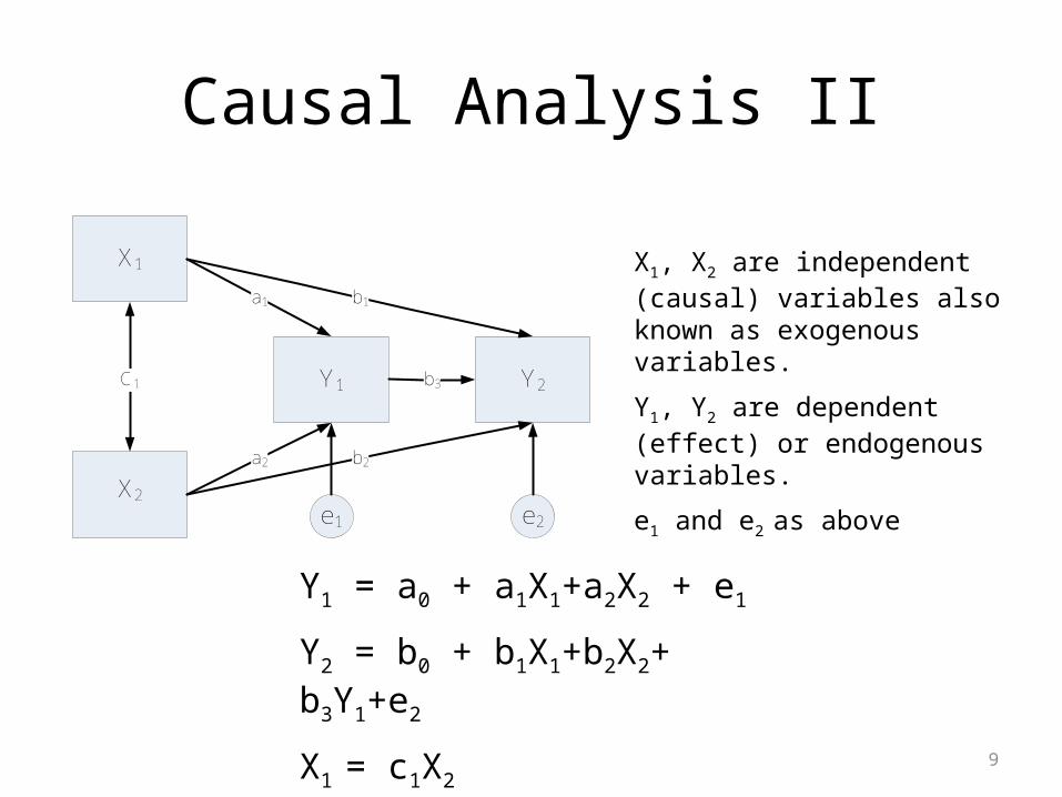
Causal Analysis II

X1, X2 are independent (causal) variables also known as exogenous variables.

Y1, Y2 are dependent (effect) or endogenous variables.

e1 and e2 as above

Y1 = a0 + a1X1+a2X2 + e1

Y2 = b0 + b1X1+b2X2+ b3Y1+e2

X1 = c1X2

Y2Y1

X1

X2

C1

a1 b1

a2 b2

b3

e1 e2

Root cause analysisRoot cause analysis is a structured process for reviewing an event, with the goals of determining what happened, why it happened and what can be done to reduce the likelihood of recurrence.

“On August 22nd, 2006, a 43 year old woman died after a medication incident that occurred whileshe was receiving outpatient care at the Cross Cancer Institute in Edmonton, Alberta. Thecause of death as determined by the coroner was “sequelae of fluorouracil toxicity”. On July 31,the woman had inadvertently received an infusion of fluorouracil over 4 hours that was intendedto be administered over 4 days. She was being treated for advanced nasopharyngealcarcinoma, according to a standard protocol that included high-dose fluorouracil and cisplatin inthe ambulatory setting. The medication incident was recognized within 1 hour after the infusionwas completed. The patient was admitted to hospital 4 days after the incident occurred.Profound mucositis and pancytopenia developed, and the patient experienced hemodynamiccollapse and multi-organ failure before her death.”

Source: http://www.cancerboard.ab.ca/NR/rdonlyres/4107CCF0-2608-4E4D-AC75-E4E812F94FD6/0/Incident_Report_UE.pdf

11

Herald of Free Enterprise sinking – causal analysis

ROOT CAUSE ANALYSIS of a ferry sinking

12

The mother of all causal diagrams

A PowerPoint diagram that portrays the complexity of American strategy in Afghanistan as having succeeded.

http://www.nytimes.com/2010/04/27/world/27powerpoint.html?src=me&ref=general

Concept of causality

• Causality often implies inevitability, but the reality is that causal statements usually reflect degrees of uncertainty.

• Causality and probability are fundamentally connected because we want to :– Know the causes of an event– Measure the relative strength of these causes

Randomized experiments

• Classic experiment is the random, double-blind experiment (RDE):– subjects are selected randomly into a treatment

and control group– each subject received a code– an independent third party assigns codes

randomly to treatment and control group members.

– the treatment is not identifiable (i.e., the real and fake pill are identical.

– those administering the treatments and placebo have no knowledge of what subject receives.

Key benefits of the RDE

• randomization creates statistically equivalent groups

• in the absence of any interventions (the drug under tests), the incidence of disease is the same for both groups

• the groups are the “same” (statistically, except that one gets the drug and the other a placebo

• analysis can be done by difference of means tests or other basic techniques.

Limits of RDE

• In social science, randomized double blind experiments are often not feasible:– human subjects are unreliable (they move, die

or otherwise fail to participate in the full experiment).

– many see the administration of a placebo as withholding a treatment.

– social policy cannot be masked (creating a placebo is difficult).

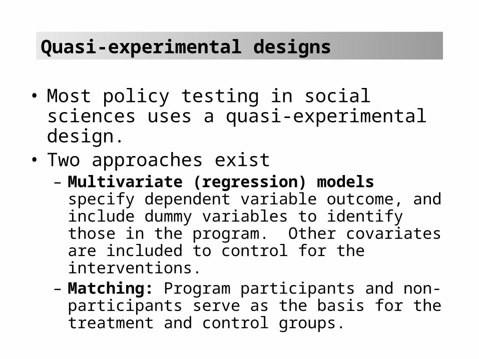
Quasi-experimental designs

• Most policy testing in social sciences uses a quasi-experimental design.

• Two approaches exist– Multivariate (regression) models specify dependent

variable outcome, and include dummy variables to identify those in the program. Other covariates are included to control for the interventions.

– Matching: Program participants and non-participants serve as the basis for the treatment and control groups.

Four potential models for evaluating policy

1. Randomized control (RC)

2. Natural experiments (difference-in- difference, discontinuity)

3. Quasi-experimental methods– Heckman two step– Statistical Matching

4. Instrumental variables (treated separately)

Randomized control

Attempts to create a situation where

Cov (X’, ) = 0, or

E(T’, ) = E(T”, W), where W are the omitted variables that determine selection into treatment.

Natural experiments

• Create a “split” in the sample, where treated and untreated are classified by a variable that is not related to the the treatment.

• This split occur “naturally” where the program change occurs in one area/jurisdiction, not in others that are “closely similar.”

• Difference-in-differences (DID) methods are a common evaluation framework.

Difference in Differences

• The DID estimator uses the average before and after values for an outcome variable for the program and comparison group.

DID = [Yp (t=a) – Yp(t=b) ] – [Yc

(t=a) - Yc(t=b) ]

• Example:– Avg. earned income before - program group = $4500– Avg. earned income after - program group = $6500– Avg. earned income before - comparison group = $10,500– Avg. earned income after - comparison group = $11,000

DID = [6500 - 4500] – [11,000 – 10,500] = $1,500

= net impact attributable to the program (treatment)

Net impact using DID

Yp (t=a)

t=b t=a

Yc (t=a)

Yc (t=b)

Yp (t=b)

a

b

c

d

e

bc = de

Y(income,

hours, etc.)

Time

Causal Inference – comparison in regression

Problem: Estimate effect of treatment (T) on observed outcome (Y), or estimate B in

Yi = B0 + B1Ti + i = Xi B + I (where X = [1, T]Assume

– dichotomous treatment variable: T=1 if treated, 0 otherwise– homogeneous treatment effect (B) (every i experiences

same effect) “average treatment effect”– Linear (no dose)– no covariates mediate the outcome

Bhat = Ybar(T=1) – YBar (T=0)

T = 1 (treatment) = 0 otherwise Y

i

B

The simple comparison group model

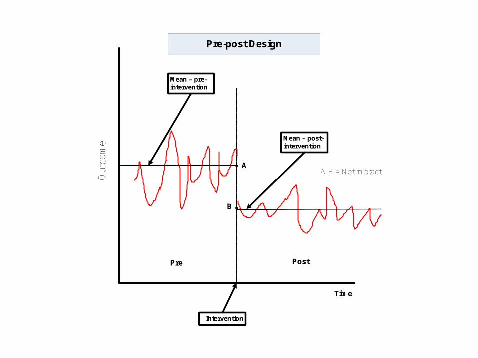
Mean – pre-intervention

Mean – post-intervention

Time

Intervention

Pre Post

A

B

A-B = Net imp;act

Pre-post Design

Out

com

e

OLS assumption E (X’, ) = 0, or

E (X’, ) = X’ (Y- BOLSX)

which then creates the OLS estimator

BOLS = (X’X) –1 X’y

But, with omitted variables, the validity of OLS requires the omitted variables to be uncorrelated with T (the treatment). This is the essence of the self-selection problem.

No covariates is the key assumption

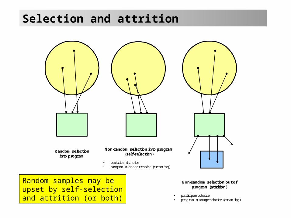
Selection and attrition

Random selectioninto program

Non-random selection into program(self-selection)

participant choice program manager choice (creaming)

Non-random selection out ofprogram (attrition)

participant choice program manager choice (creaming)

Random samples may be upset by self-selection and attrition (or both)

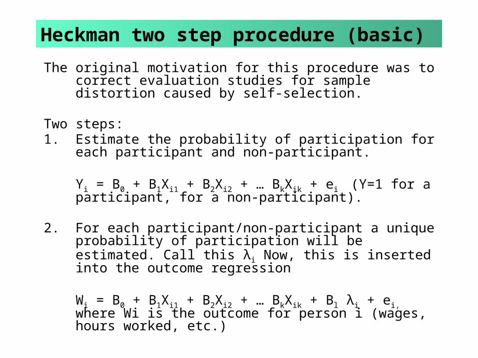
The original motivation for this procedure was to correct evaluation studies for sample distortion caused by self-selection.

Two steps:1. Estimate the probability of participation for each participant

and non-participant.

Yi = B0 + B1Xi1 + B2Xi2 + … BkXik + ei (Y=1 for a participant, for a non-participant).

2. For each participant/non-participant a unique probability of participation will be estimated. Call this λi Now, this is inserted into the outcome regression

Wi = B0 + B1Xi1 + B2Xi2 + … BkXik + Bl λi + ei, where Wi is the outcome for person i (wages, hours worked, etc.)

Heckman two step procedure (basic)

Matching

In social experiments, participants differ from non-participants because:– failure to hear of program– constraints on participation or completion– selection by staff

Matching participants and non-participants can be accomplished via– pair-wise– statistical

Matching Process

PARTICIPANTS

NON-PARTICIPANTS

MatchingProcess

Pairwise Statistical

PROGRAMGROUP

COMPARISONGROUP

Pair wise matching

• The theory will indicate those attributes that are likely to make a difference in the quasi-experiment.– For labour markets, gender, education and rural-

urban location are important– For health policy, age, rural-urban, and family

history might be important.

• The analyst starts with the first variable, and divides the participants and non-participants into two sets.

• Within the sets the samples are classified with respect to the second, variable and so on.

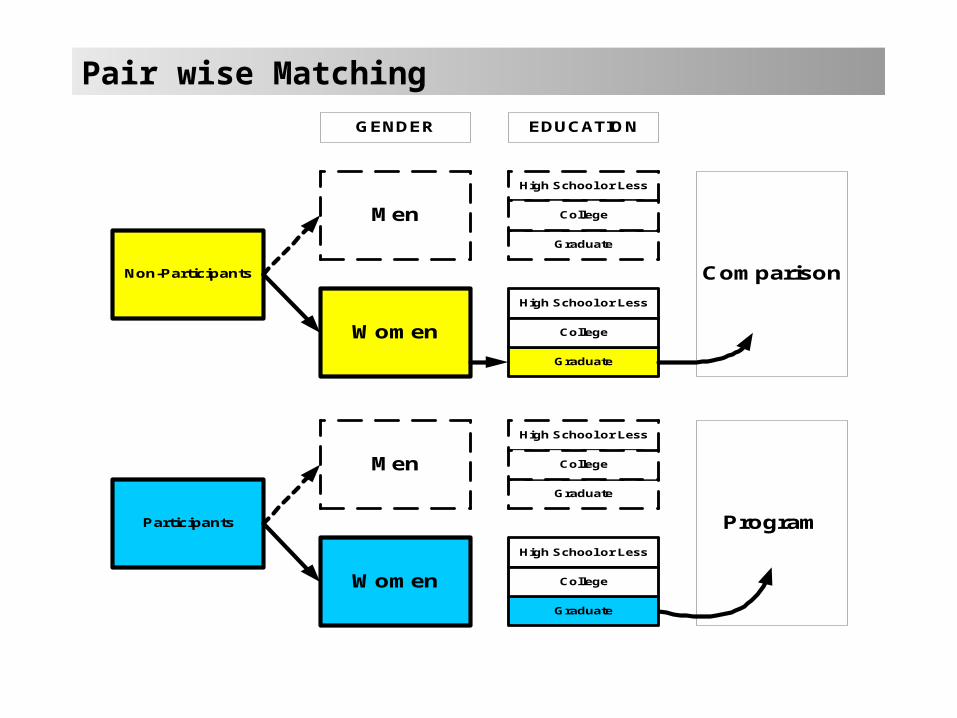
Non-Participants

Men

Participants

Men

Women

Women

Graduate

High School or Less

College

Graduate

High School or Less

College

Comparison

Program

GENDER EDUCATION

Graduate

High School or Less

College

Graduate

High School or Less

College

Pair wise Matching

Statistical Matching

• Matching is needed because we cannot randomly allocate clients to the program and comparison groups. Program benefits cannot be withheld.

• Logit model provides the estimate of the propensity to participate for participants and non-participants.

• The key idea is that we estimate that propensity to participate is based on observed attributes of the participants and non-participants.

• Participants are assigned a “Y”value of 1 and non-participants are assigned a “Y” value of 0.

• A logistic regression then estimates the propensity to participate.• Note that even though a non-participant actually did not participate the

model will assign a score between 0 and 1. Typically non-participants will have lower scores than participants, but there will be an overlap.

• The overlap is termed the region of common support.

Rationale for statistical matching

• Matching is needed because we cannot randomly allocate EI clients to the program and comparison groups. Part II benefits cannot be withheld.

• Logit model provides the estimate of the propensity to participate for participants and non-participants.

• The key idea is that we estimate that propensity to participate is based on observed attributes of the participants and non-participants.

• Participants are assigned a “Y”value of 1 and non-participants are assigned a “Y” value of 0.

• A logistic regression then estimates the propensity to participate.• Note that even though a non-participant actually did not participate the

model will assign a score between 0 and 1. Typically non-participants will have lower scores than participants, but there will be an overlap.

• The overlap is termed the region of common support.

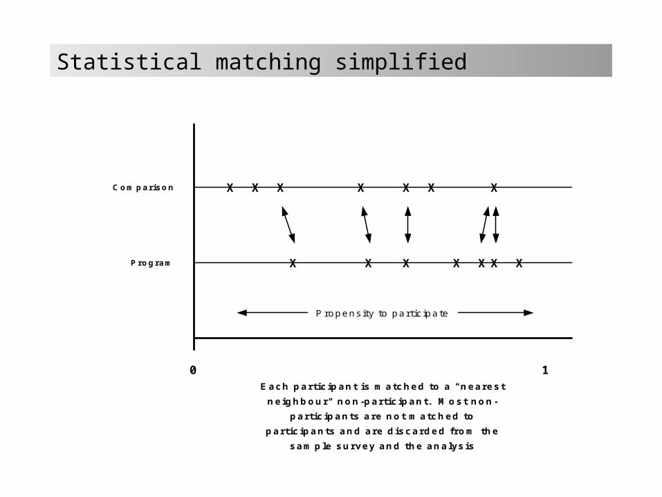
Statistical matching simplified

0 1

Program

Comparison

X X X X X XX

X X X X X X

Each participant is matched to a "nearestneighbour" non-participant. Most non-

participants are not matched toparticipants and are discarded from the

sample survey and the analysis

Propensity to participate

X

The logit model

LPM Model Pi = E(Y = 1| Xi)

= B1 + B2X2 + B3X3 +..+BkXk

Logit Model Pi = E(Y = 1| Xi)

= 1/[1+ e – (BiXi)]

In Log Odds format

Li = ln(Pi/1-Pi) = Zi = BiXi

Region of Common Support

• Each participant has the value of 1 for P and each non-participant has the value 0.

• However, once the model is estimated, each participant and non-participant has a score between 0 and 1. Participants tend to have scores closer to 1 and non-participants are closer to 0.

• The distribution of scores can be graphed.

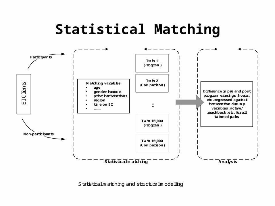
EI

Clie

nts

Participants

Non-participants

Matching variables age gender income prior interventions region time on EI ......

Statistical matching

Twin 1(Program)

Twin 2(Comparison)

Twin 10,000(Program)

Twin 10,000(Comparison)

:

Difference in pre and postprogram earnings, hours,

etc. regressed againstintervention dummy

variables, active/reachback, etc. for all

twinned pairs

Analysis

Statistical matching and structural modelling

Statistical Matching

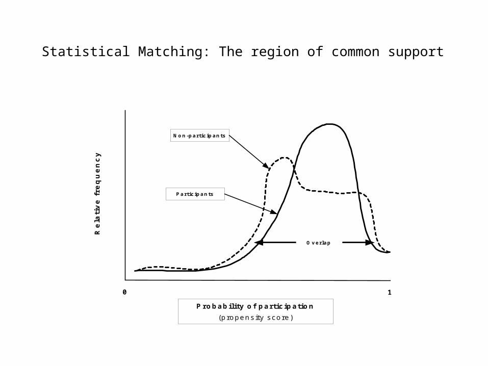
Statistical Matching: The region of common support

0 1

Probability of participation(propensity score)

Participants

Non-participants

Overlap

Re

lati

ve

fre

qu

en

cy

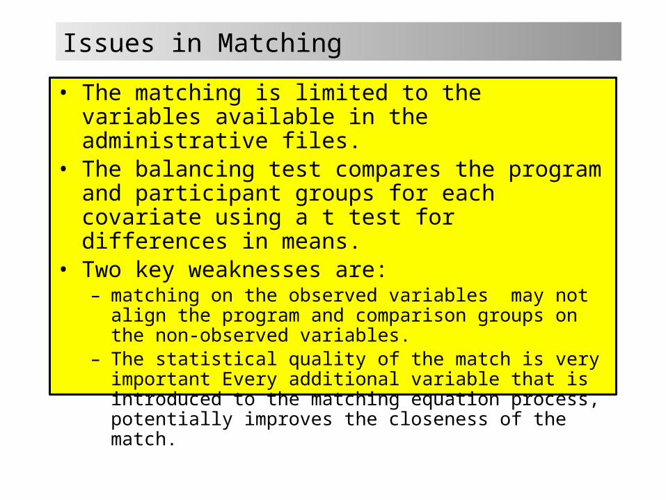
Issues in Matching

• The matching is limited to the variables available in the administrative files.

• The balancing test compares the program and participant groups for each covariate using a t test for differences in means.

• Two key weaknesses are:– matching on the observed variables may not align the

program and comparison groups on the non-observed variables.

– The statistical quality of the match is very important Every additional variable that is introduced to the matching equation process, potentially improves the closeness of the match.

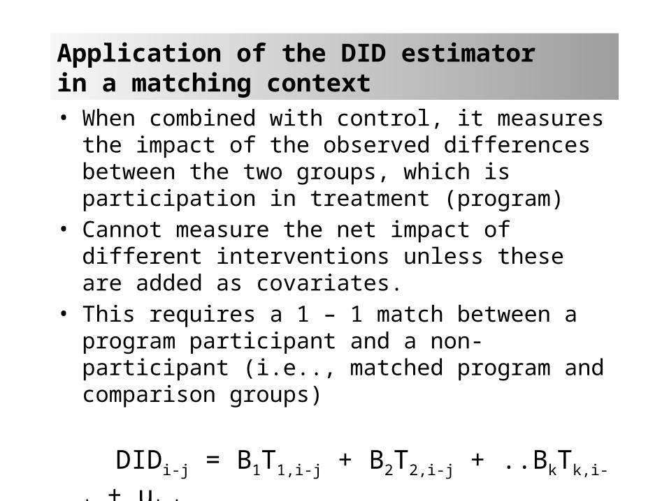
Application of the DID estimatorin a matching context• When combined with control, it measures the impact

of the observed differences between the two groups, which is participation in treatment (program)

• Cannot measure the net impact of different interventions unless these are added as covariates.

• This requires a 1 – 1 match between a program participant and a non-participant (i.e.., matched program and comparison groups)

DIDi-j = B1T1,i-j + B2T2,i-j + ..BkTk,i-j + ui-j

Effect of training programs – wages and hours increase

Measures of outcome• Increase in earnings (I)• Increase in hours (I)• Reduction in social assistance payments

(G)• W0 = market wage at ho and W1 = market

wage at h1

• Increase in surplus arises from increase in market wages and increase in hours)

A is the net increase due to wage increase at old hours

B = C is the increase in hours times the new wage

C = loss of leisureIf individuals were under-employed or find

virtue in work, then C is part of the social surplus. If individuals value leisure but cannot regulate the time they work (a fixed work day/week).

Labour supply

Effect of training programs – hours increase

When only hours increase, the social surplus lies above the supply survey (and below the wage rate).

Market wages remain stable.

Note the similarity with the concept of producer surplus.

Workfare This policy requires a minimum number of hours (h*, where h* = grant/min wage)

Wm is the min wage which is assumed to be equal to the market wages associated with S0 and S1.

The reservation wage is the payment needed to bring forth one hour of work … W0

r and W1r

If the policy reduces/eliminates social assistance payments, then labour supply shifts right (S0 – S1).W1

r falls below the min wage. The recipient if offered h* hours at Wm