COMPUTER METHODS IN APPLIED MECHANICS AND ENGINEERING 49 (1985) 175-201 NORTH-HOLLAND HIGHER-ORDER UPDATES FOR DYNAMIC RESPONSES IN STRUCTURAL OPTIMIZATION Azhar H. JAWED and A.J. MORRIS College of Aeronautics. Cranfield Institute of Technology, Cranfield, Bedford MK43 OAL, U.K. Received 26 March 1984 Problems of structural re-analyses in design optimization with constraints on the vibration response of dynamically loaded structures have been addressed. The inherent nonlinearity of the response quantities with respect to the design variables has in the past limited the application to first-order natural frequency updates. Second-order methods have tended to be prohibitive because of the need to evaluate the natural modes (eigenvectors) updates. The method proposed adopts an alternate and more direct approach to the forced vibration problems by evaluating the nodal response updates in a given direction. The update formulation developed takes advantage of the mutual orthogonality of the natural modes to construct higher-order directional derivatives of the transformed co-ordinate (modal) response quantities. These are sub- sequently used to obtain a total summation of the Taylor series representation for the response updates. The formulation is particularly suited to the design of large structures where modal truncation can be employed to restrict the computational costs. Numerical examples have been provided to illustrate both the higher quality and the effects of modal truncation on the results. 1. Introduction Requirements for computing response derivatives in structural design optimization studies stem from a variety of applications. Many of the successful and efficient multivariate, nonlinear programming algorithms make use of first- and/or second-order derivatives of both the objective and constraint functions during each cycle of the iteration process. In addition these derivatives can form the basis for performing design sensitivity analyses, which provide the necessary information for advantageous redesign. This philosophy can be applied either before or after the optimization process in order to assess the dependence of the behaviour characteristics on the problem parameters. Optimization and design synthesis are iterative processes and require repeated evaluation of the objective and constraint functions together with their partial derivatives. The efficiency of the procedure is, therefore, dominated by the cost of such evaluations. One of the major stumbling blocks is the representation of the behaviour constraints which are invariably implicit, nonlinear functions of the design variables. A finite element representation of even a modestly sized structure may involve many hundreds of degrees of freedom and element representation. Cost effectiveness in solving problems of a practical scale and complexity can only be obtained when this effort is minimized by utilizing approximate ‘re-analysis’ for- mulations which help in identifying active/inactive constraint sets. In the context of re-analyses 004%7825/85/$3.30 @ (1985), Elsevier Science Publishers B.V. (North-Holland)

Welcome message from author
This document is posted to help you gain knowledge. Please leave a comment to let me know what you think about it! Share it to your friends and learn new things together.
Transcript
COMPUTER METHODS IN APPLIED MECHANICS AND ENGINEERING 49 (1985) 175-201
NORTH-HOLLAND
HIGHER-ORDER UPDATES FOR DYNAMIC RESPONSES IN STRUCTURAL OPTIMIZATION
Azhar H. JAWED and A.J. MORRIS College of Aeronautics. Cranfield Institute of Technology, Cranfield, Bedford MK43 OAL, U.K.
Received 26 March 1984
Problems of structural re-analyses in design optimization with constraints on the vibration response
of dynamically loaded structures have been addressed. The inherent nonlinearity of the response quantities with respect to the design variables has in the past limited the application to first-order
natural frequency updates. Second-order methods have tended to be prohibitive because of the need to evaluate the natural modes (eigenvectors) updates.
The method proposed adopts an alternate and more direct approach to the forced vibration problems by evaluating the nodal response updates in a given direction. The update formulation developed takes advantage of the mutual orthogonality of the natural modes to construct higher-order directional derivatives of the transformed co-ordinate (modal) response quantities. These are sub- sequently used to obtain a total summation of the Taylor series representation for the response updates. The formulation is particularly suited to the design of large structures where modal truncation can be employed to restrict the computational costs. Numerical examples have been provided to illustrate both the higher quality and the effects of modal truncation on the results.
1. Introduction
Requirements for computing response derivatives in structural design optimization studies stem from a variety of applications. Many of the successful and efficient multivariate, nonlinear programming algorithms make use of first- and/or second-order derivatives of both the objective and constraint functions during each cycle of the iteration process. In addition these derivatives can form the basis for performing design sensitivity analyses, which provide the necessary information for advantageous redesign. This philosophy can be applied either before or after the optimization process in order to assess the dependence of the behaviour characteristics on the problem parameters.
Optimization and design synthesis are iterative processes and require repeated evaluation of the objective and constraint functions together with their partial derivatives. The efficiency of the procedure is, therefore, dominated by the cost of such evaluations. One of the major stumbling blocks is the representation of the behaviour constraints which are invariably implicit, nonlinear functions of the design variables. A finite element representation of even a modestly sized structure may involve many hundreds of degrees of freedom and element representation. Cost effectiveness in solving problems of a practical scale and complexity can only be obtained when this effort is minimized by utilizing approximate ‘re-analysis’ for- mulations which help in identifying active/inactive constraint sets. In the context of re-analyses
004%7825/85/$3.30 @ (1985), Elsevier Science Publishers B.V. (North-Holland)
176 A.H. Jawed, A.J. Morris, Higher-order updates for dynamic responses
procedures a Taylor-series representation is often used in obtaining the updates of the behaviour constraints. This aspect has been employed for design optimization under both static as well as dynamic loading conditions. In addition re-analysis techniques based on perturbation methods have also been presented in the literature [l, 2,3, 71. However, this
approach is not particularly suited to optimization schemes as it requires repeated evaluation of the perturbed global coefficient matrices and matrix solutions for multiple right-hand sides.
All approximate techniques are accurate only within a neighbourhood of the base design point at the start of the iteration cycle. Thus restrictions are imposed by move limits along the search direction within which the quality of the results can be considered acceptable. Quite obviously, the number of design iterations necessary, and hence the efficiency of the synthesis process, is dependent on the size of this ‘quality zone’ of the approximate formulations, as well as the relative computational effort involved.
In a multivariate design problem, the Taylor series makes use of mixed partial derivatives in updating the behaviour functions for design-variable changes in a specified direction. Use of mixed derivatives makes it imperative to truncate the series for reasons of computational difficulties. The accuracy of such updates naturally depends on the order of the derivatives at
which the series is truncated. The use of first-order updates is well established for both static and dynamic [4,6] response quantities. The inherent nonlinearity of the response functions, however, permits a very limited quality zone in a linearized representation. In special cases of static response behaviour the problem can be alleviated by using inverse design variables. For dynamical response quantities, however, it has been shown [5] that simple variable trans- formation does not linearize the behaviour, and its use may in fact destabilize the search direction. In more complex configurations, use of second-order mixed derivatives has been suggested [5] but the cost of constructing the full Hessian matrix can become prohibitive, both from the computational and storage view point. An attempt to alleviate this problem for static response quantities was presented by Jawed and Morris [8] by considering higher-order directional derivatives. The present work attempts to extend the concept to the dynamical behaviour of structures.
The paper aims at developing a high-quality formulation for evaluating forced response updates for undamped, dynamically loaded structures under harmonic excitation, for use in line-search techniques. The method reduces the computational effort by considering direc- tional derivatives which permit much larger move limits along the search direction. In fact, the procedure is particularly suited to the design of a large (degrees of freedom) system, where a truncated modal analysis can be performed to restrict the analysis to any desired number of lower modes.
The presentation begins by considering the expression for the modal response functions for an undamped multi-degree of freedom structure, suitably discretized using finite element modelling. The general higher-order directional derivatives of the response functions are then used to construct a series expression for the response updates. The paper proceeds, in Section 3, to formulate the expression for approximate updates, which ensures convergence of the series by utilizing the orthogonality of the eigenmodes. An expression for the response derivatives with respect to design variables (gradient vector) has also been derived. What is significantly noteworthy is that the computational effort needed in obtaining the expression for the convergent series is based entirely on first-order information only. This makes the ‘modal update’ formulation, presented herein, very economical and particularly suited in a design
A.H. Jawed, A.J. Morris, Higher-order updates for dynamic responses 177
synthesis environment. The formulation has been tested (Section 4) against example problems where a given structure, representing the base design point, is sequentially modified along a pre-determined line. Problem variations to include a wide excitation-frequency range, and modal truncation for large (degrees of freedom) structures have also been considered. Comparisons of the approximate and exact analyses at re-design points demonstrate the accuracy and suitability of the modal update technique.
In the present development for approximate re-analysis of dynamic systems, only undamped structures have been considered. However, extension of the approach to include damping should be possible without difficulty.
2. Problem statement
Undamped nongyroscopic dynamical systems are characterized by real symmetric mass and stiffness matrices; where the mass matrix is positive definite and the stiffness matrix is either positive definite or positive semi-definite. If appropriate boundary conditions are applied, the rigid-body degrees of freedom can be eliminated. The equations of motion for the system can be represented in matrix form as:
(1)
where [M] and [K] are the real symmetric mass and stiffness matrices, {q(t)} is an n-vector of nodal displacement response, and {Q(t)} is the n-vector of dynamic loads. For a harmonic excitation, (1) simplifies to
where n (rad/sec) is the forcing or excitation frequency, and {zi} and {F} represent the amplitude vector of the nodal displacements and the system excitation respectively; (it is assumed here the excitation at all points are in phase and at a constant frequency 0).
Equation (2) represents a system of linear equations which can be directly solved for the unknown displacement vector to give the forced response. Defining the global dynamic stiffness matrix [Z] :
PA = WI - ~‘PfI> 3
:. {U} = [z]-‘(F). (34
Assuming the element coefficient matrices to be a linear function of the design variables, and the value of L? is such as not to make the dynamic stiffness matrix singular, the general pth-order directional derivative of the displacement amplitudes can be expressed as [6]:
a(P)fi
I I - = (- l)P(p!)([z]-'[az/aa]P{ff} , aa (p) (4)
178 A.H. Jawed, A.J. Morris, Higher-order updates for dynamic responses
where cu represents a step-length parameter which determines the distance moved along a search direction in the design space; i.e.
Equation (5) defines a line in an N-dimensional hyper-space which describes the direction along which design modifications are made. ~5%~ are the elements of the search vector, and the superscript (cr) indicates the values of the design variables at each successive step starting at the base design (indicated by the superscript (0)). The Taylor-series representation for the response updates for the displacement amplitude vector is given by:
Substituting for the derivative terms from (4)
With the series expression within the outer brackets representing a binomial expansion, the above equation reduces to:
{zz’“‘} = g--9,] -I- [z]-‘[c?z/&Y])-l{ii’o)}. (7)
Equation (7) is similar to that obtained, based on perturbation methods, by Kitis, Wang and Pilkey [7]. An additional coefficient matrix to account for damping effects has also been included in their study. The solution technique adopted in [7], however entails matrix solution at each re-design, and is not suited to an optimization scheme. Re-analysis techniques based on high-order perturbation methods do exhibit improved accuracy over truncated Taylor series. However, using directionaf derivatives to obtain (7) enables the inclusion of all higher-order terms and convergence of the series. Thus, depending on the representation of the matrix product [Z]-‘[~Z/&_X] the level of accuracy can be maximized. More significantly, the form of (7) is amenable to design optimization studies as it lends itself directly to line-search techniques. Unlike a perturbation-based formulation, where repeated evaluation of the perturbed coefficient matrix and matrix solution is necessary at each stage of design modification, use of directional derivatives necessitates only a single (approximate) evaluation of the matrix product in (7). Furthermore, after a total series summation has been achieved, the formulation reduces to one where only the first-order derivations are needed.
A.H. Jawed, A.J. Morris, Hugger-order ~~a~e~ for dy~a~jc responses 179
In [8] where only statically loaded structures are considered, the effort in computing the updates is further economized by using approximate mimic derivatives which diagonalized the matrix product term. This approach can be extended to the present study. However, a more elegant approach which exploits the characteristics of the structural behaviour has proved advantageous for dynamically loaded structures.
3, SoIution strategy
The approach for diagonajizing the product matrix in (7) adopts the modal analysis technique using the mutual orth~gonality of the natural modes (eigen vectors) of free vibrating structures, Although this precludes an eigensolution, needed once at the base design point during each interaction cycle, it is not considered to be a computational burden. Evaluation of the natural frequencies and mode shapes is an essential step in the synthesis of dynamically loaded structures. Moreover, for the system defined by (l), the response due to any general- ized excitation can also be conveniently obtained by modal analysis. Due to the special nature of such systems, the response is obtained with relative ease when compared to the di~culty involved in obtaining the response of a general dynamical system. This advantage becomes more apparent when the order of the system increases, as the eigen-analysis can be restricted to any desired number of mode shapes by employing modal t~ncation. It is thus presumed that the eigen-information necessary for the update analysis presented herein is available.
The eigenva~ue problem associated with (I) is:
where Ai and {Vi} are the eigenvalues and the associated eigenvectors respectively. Because [K] and [Mf are real, symmetric and positive definite, all the eigenvalues are real and positive, i.e.
&=wf (i= l,...,it), (9)
where ai are the natural frequencies of the systems and are assumed to be distinct. The eigenvectors are all mutually orthogonal. If they are normalized with respect to the global mass matrix, then the orthonorma~ity of the eigenvectors can be expressed as:
where {zi} represents the normalized eigenvectors, and 6, is the Kronecker delta which assumes the foI~owing values:
s = 1 for i=j, @ 1 0 for i+j.
180 A.H. Jawed, A.J. Morris, Higher-order updates for dynamic responses
Premultiplying (8) by {S};, it follows that
Introducing the truncated modal matrix comprising of 1 number of orthonormal eigenvectors:
Equations (10) and (12) can be written as:
where [‘r,] is the identity matrix and PA,] is an I x 1 diagonal matrix of system eigenvalues with the rth diagonal element corresponding to the rth eigenvalue, i.e.
A, = A, = 6J’r (r = 1, . . 1) I) 1
Defining a linear transformation of response amplitudes:
where {$} represents an I-vector of independent generalized principal co-ordinates. Pre- multiplying (2) by (@)‘, and using (14) the equations of motion are uncoupled and reduce to a diagonalized form.
[Y?$“.] represents the diagonalized coefficient matrix, and {a is the transformed load amplitude vector. The obvious advantage of decoupling the equations of motion is that the generalized co-ordinates (3) can be determined independently without recourse to the assembly and factorization of the global dynamic stiffness matrix. The system response can then be obtained using (15).
For the purpose of performing an update analysis, (13)-(16) are used to transform (1) to a set of 1 independent decoupled equations. It is presupposed that an eigen- and modal analysis is performed at the start of each iteration cycle, which thus forms the base design for a line search in an N-dimensional space. The sequential design modifications are controlled by the step-length parameter cy (Equation (5)), which determines the extent of modification in- corporated in the design variables for each successive re-analysis.
3.1. Modal update analysis
Returning to (13), it can be seen that since the set of eigenvectors {&}, i = 1, . . . , 1 are all mutually orthogonal, they form a generating system of non-zero, linearly independent vectors in an L’ space. In the formulation development that follows, the IZ x E modal matrix (Sp) thus becomes a convenient choice as an orthogonal basis in the design space, and is considered
A.H. Jawed, A.J. Mom’s, Higher-order updates for dynamic responses 181
invariant over the range of moves, determined by the desired the response updates can then be represented as:
{ii’“‘} = {@}{jj(“l)},
where {+‘p’} is a vector of updates along the generalized successive step, for a specified value of cy.
From (14) and (16), and using the superscript (0) to indicate
{@>‘[Z(“)]{@} = [--%C._]
defining a pseudo-inverse {@)’ of the truncated modal matrix,
WI’{@] = L’Z.1 and {@)‘{@p)” = [‘Z.] ,
[Z(O)] = {@)+~[~2T’“~]{@)’ ,
:. [z(o)]-1 ={@}[Y’Jq-l{@j>t.
Re-arranging (7) and using (17) and (19)
limiting value of (Y. From (15)
(17)
co-ordinate direction at each
values at the base design point
US)
such that:
(19)
{@}{?p’} = ([.Z.] + cy{~}[~~~]-‘{~)‘[azo/a(y])~~~{jj(”)} ;
pre-multiplying by {CD}
or {@)+{@}{ij’“‘} = ({@+{@} + a{@}+{@}[YeL_]-‘{@)‘[az”)/af2]){@}{ij~”~} ;
{7j?} = [‘Z.] + CX[ 3!(O) (
]- 1 [LS\]) -‘{+o’) )
where the diagonalized derivative matrix is defined as:
[\C!gJ.TJ.T] 3 {@>‘[az’“‘/aa]{@}.
(20)
(21)
Equation (20) gives the updates for the generalized co-ordinates for moves made along the search direction, as an explicit function of the step-length parameter. The diagonalized form of the coefficient matrix inverse and the derivative matrix, conveniently decoupled the equations and no matrix inversion is needed. Furthermore, by employing modal truncation the solution of extremely large problems can also be conveniently handled.
The terms of the diagonalized matrices are easily obtained:
. .
Similarly,
(Y~O))-l = dia[Y%‘$?,]-’ = dia([‘ll $,I - a’[‘-Z,])-’ ,
(2zy)-1 = l/(A !“’ - 02) .
from (21):
(22)
182 A.H. Jawed, A.J. Mom’s, Higher-order updates for dynamic responses
Substituting (3a) in the above expression:
[~~~]= N , 2 w>‘; WO’l - .n’[M(“‘]){@}sx;
N
= 2 {@y([k!“] - O*[m p)]){@}Sxi/xi , i=l
where [k$“] and [m$‘] are the stiffness and mass matrices respectively for the ith element at the base design point. The rth term of the diagonalized derivative matrix is:
z = dia[\zL] = i (G,,):([k$“)] - fi*[m p)])(+,), $! .
{Gad, represents a vector whose elements are extracted from the rth eigenvector corresponding to the nodal directions of the ith element. Defining:
1 h(i), E - { 6cij)‘ik P’]{ s,iJ,
Xi
and
(234
Au,l and p(i)r represent the maximum strain and maximum kinetic energy respectively for the ith element, with the structure vibrating in its rth natural mode. It may be noted that for the mass-normalized eigenvectors:
N
i=l and 2 X+(i), = 1 .
i=l
Using (23) the diagonal element of the derivative matrix can be represented as:
8%$‘)/@3a = (h(i), - fJ*/A(i),)SXi * i=l
Substituting (22) and (24) in (20), the rth generalized co-ordinate update becomes
(24)
W-4
Evaluating all the (1) terms of the generalized co-ordinate update vectors, the nodal response
A.H. Jawed, A.J. Morris, Higher-order updates for dynamic responses 183
amplitudes are readily recovered from
{ZP’} = {@}{?p’} . (23
3.2. Response gradients
First-order partial derivatives (gradient) of the constraint functions provide information for advantageous re-design and help to define appropriate changes in the design variables (search direction) as the design synthesis proceeds towards an optimum solution. The task of efficiently obtaining constraint gradients {VC}, based on the previous analysis, will now be addressed.
The gradient vector for a constraint representing the jth nodal response amplitude is:
{Vg), = {Vii,)t = {$Z, . . . ) $1. I 2 N
(26)
From (4) the first-order derivative of the response functions with respect to the ith design variable is:
aii 1 I - =- dXj
[Z]_‘[az/ax,]{fi} . (27)
Using expressions for the dynamic stiffness matrix inverse and derivative matrix from (19) and (21), in the above equation
aii I 1 -_= i?Xj
-{~}[~~.]-‘{aS>t{~}+t[-a~/aX~_]{~}{~} = -{~}[‘~:,]-‘[-a~/aXi-l{~} -
The inverse and derivative matrices are now conveniently diagonalized. Pre-multiplying both sides by a row vector containing a unit value at the jth location and zeros else where, the derivative for the jth nodal response amplitude can be extracted. Thus
3_ dXi
- - { ~>t[~~.]-‘[-a~/axi_]{~} ,
where { vj>t is a row vector whose elements correspond to the jth term of the 1 eigenvectors. The rth term of the diagonal matrices are obtained from (22) and (24) respectively, i.e.
- { Vj:.>’ = {Ujl 7 uj2, . f * 9 ujt> 9
dia[--%.]-’ = l/(h, - a’), r = 1, . . . ,1, (29)
where A(i), and p(i)r are defined by (23).
1x4 AX Jawed, A.J. Mo~is, Higher-order updates for dynamic responses
Substituting the various terms from (29) in (ZS), the ith element of the jth response gradient vector becomes:
A comparison of (25) and (30) indicates that the modal update formulation is based entirely on first-order information.
4. Numerical examples
In order to demonstrate the accuracy of the update fo~ulation, (25) was tested on example problems ranging from a simple 3-element, two-degrees of freedom (d.o.f.) system to a more realistic 69-element, 60-d.o.f. structure representing a helicopter tail. The dynamic system defined considers an undamped structure subjected to harmonic excitations only; the object of the exercise being, primarily, to assess the efficiency and usefulness of the approximate re-analysis formulation in a design synthesis environment.
The search vector, in the exampfes, have been chosen arbitrarily to maintain the generality of the fo~ulation. The extent of design changes incorporated at each stage of the search is determined by a single (step-length) parameter C-Z. The % average change per element (Ax) in the design variables can be expressed as:
(31)
where SX, are the elements of the direction vector.
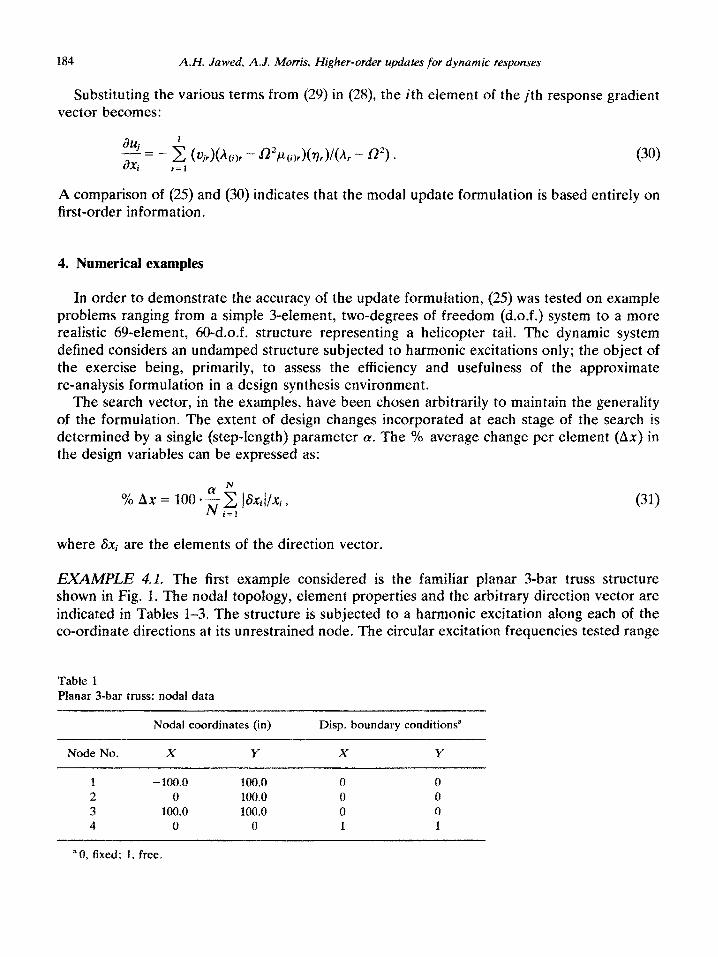
EXAMPLE 4.1. The first example considered is the familiar planar 3-bar truss structure shown in Fig. 1. The nodal topology, element properties and the arbitrary direction vector are indicated in Tables 1-3. The structure is subjected to a harmonic excitation along each of the co-ordinate directions at its unrestrained node. The circular excitation frequencies tested range
Table 1
Planar 3-bar truss: nodal data
Nodal coordinates (in) Disp. boundary conditions”
Node No. X Y X Y
1 -100.0 100.0 0 0 2 0 100.0 0 0 3 100.0 100.0 0 0
4 0 0 1 1
“0, fixed; 1, free.
A. H. Jawed, A. J. Morris, Higher-order updates for dynamic responses 185
Table 2 Planar S-bar truss: loading data
No. of Load amplitude loaded nodes Node No. X-Comp. Y-Comp.
1 4 14.142 14.142
Table 3 Planar 3-bar truss: element data
Initial Nodat area
Element No. connection (in”)
1 1-4 2.0 2 2-4 2.0 3 3-4 2.0
Direction vector
(in”)
-0.2426 -0.3426 -0.2426
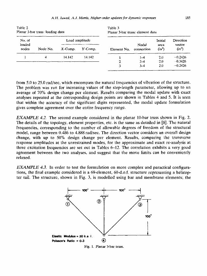
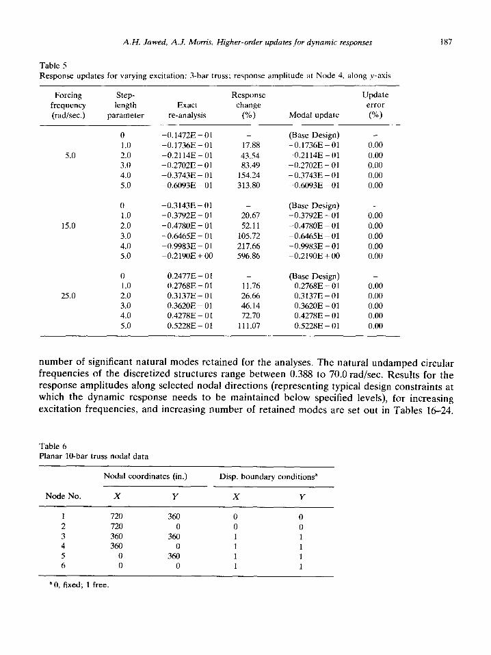
from 5.0 to 25.0 radlsec, which encompass the natural frequencies of vibration of the structure. The problem was run for increasing values of the step-length parameter, allowing up to an average of 70% design change per element. Results comparing the modal update with exact analyses repeated at the corresponding design points are shown in Tables 4 and 5. It is seen that within the accuracy of the significant digits represented, the modal update formulation gives complete agreement over the entire frequency range.
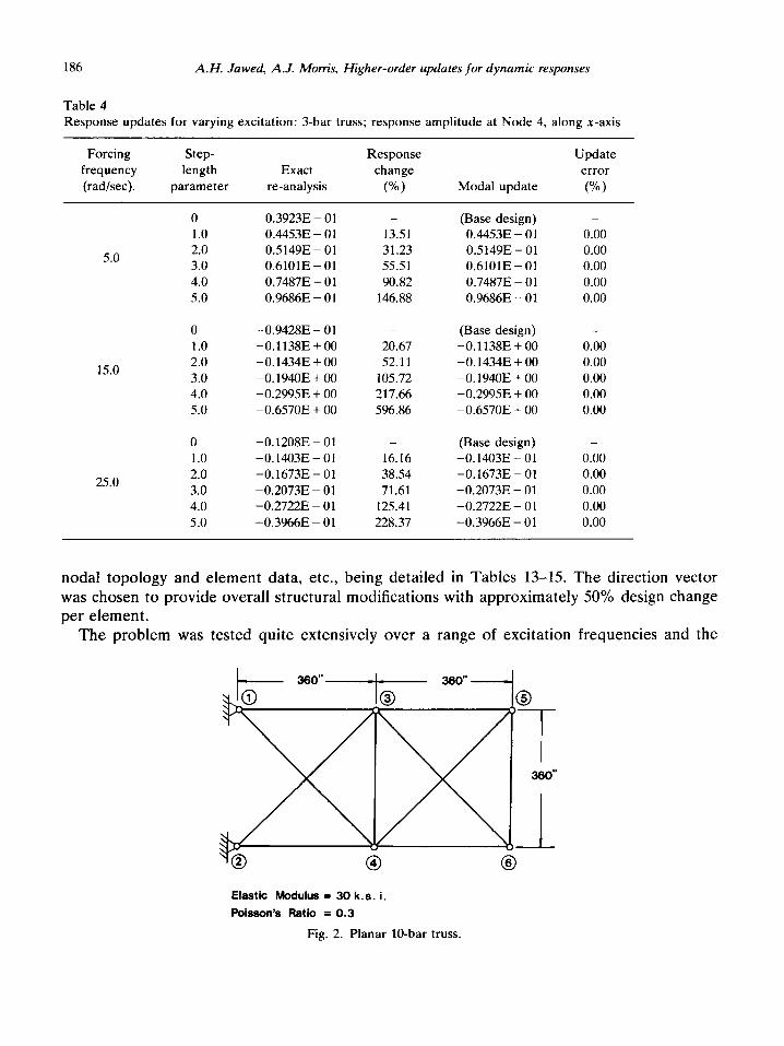
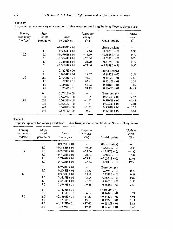
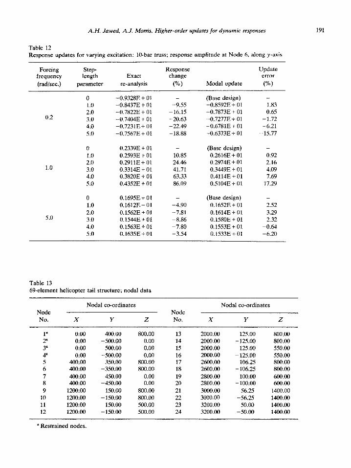
EXA~~~~ 4.2. The second example considered in the planar lo-bar truss shown in Fig. 2. The details of the topology, element properties, etc. is the same as detailed in [S]. The natural frequencies, corresponding to the number of allowable degrees of freedom of the structural model, range between 0.486 to 4.888 radlsec. The direction vector considers an overall design change, with up to 50% design change per element. Results, comparing the transverse response amplitudes at the unrestrained modes, for the approximate and exact re-analysis at three excitation frequencies are set out in Tables 4-12. The correlation exhibits a very good agreement between the two analyses, and suggest that the move limits can be conveniently relaxed.
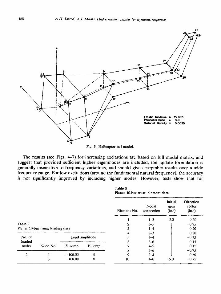
EXA~~~~ 4.3. In order to test the formulation on more complex and paractical configura- tions, the final example considered is a 69-element, 60-d.o.f. structure representing a helicop- ter tail, The structure, shown in Fig. 3, is modelled using bar and membrane elements; the
Elastic Modulus = 30 k .s i Pois5on?3 Ratio = 0.3 @
Fig. 1. Planar 3-bar truss.
Forcing
frequency (rad/sec).
5.0
15.0
25.0
186 A.H. Jawed, A.J. Mom’s, Higher-order updates for dynamic responses
Table 4 Response updates for varying excitation: 3-bar truss; response amplitude at Node 4, along x-axis
Step- length
parameter
0
1.0 2.0 3.0 4.0 5.0
0
1.0 2.0 3.0 4.0 5.0
0
1.0 2.0 3.0 4.0 5.0
Exact re-analysis
0.3923E - 01
0.4453E - 01 0.5149E - 01 0.6101E - 01 0.7487E - 01 0.9686E - 0 I
-0.9428E - 01
-O.l138E+ 00 -0.1434E + 00 -O.l94OE+ 00 -0.2995E + 00 -0.6570E + 00
-0.1208E - 01
-O.l403E- 01 -0.1673E - 01 -0.2073E - 01 -0.2722E - 01 -0.3966E - 01
Response change
W)
-
13.51 31.23 55.51 90.82
146.88
_
20.67 52.11
105.72 217.66 596.86
-
16.16 38.54 71.61
125.41 228.37
Modal update
(Base design)
04453E - 01 0.5149E 01 - 0.6101E - 01 0.7487E - 01 0.9686E - 01
(Base design)
-O.l138E+OO -0.1434E + 00 -0.1940E + 00 -0.2995E + 00 -0.6570E + 00
(Base design)
-0.1403E - 01 -0.1673E - 01 -0.2073E - 01 -0.27228 - 01 -0.3966E - 01
Update error
W)
_
0.00 0.00 0.00 0.00 0.00
-
0.00 0.00 0.00 0.00 0.00
_
0.00 0.00 0.00 0.00 0.00
nodal topology and element data, etc., being detailed in Tables 13-15. The direction vector was chosen to provide overall structural modifications with approximately 50% design change per element.
The problem was tested quite extensively over a range of excitation frequencies and the
360 -
Elastic Modulus = 30 k.s. i.
Poisson’s Ratio = 0.3
Fig. 2. Planar IO-bar truss.
A.H. Jawed, A.J. Morris, Higher-order updates for dynamic responses 187
Table 5 Response updates for varying excitation: 3-bar truss: response amplitude at Node 4, along y-axis
Forcing
frequency
(rad/sec.)
Step- length
parameter
Exact re-analysis
Response change
W) Modal update
Update error
W)
0 1.0
5.0 2.0 3.0 4.0 5.0
-0.1472E - 01 - (Base Design)
-0.1736E - 01 17.88 -O.l736E-01
-0.2114E - 01 43.54 -0.2114E - 01
-0.2702E - 01 83.49 -0.2702E - 01
-0.37438 - 01 154.24 -0.3743E - 01
-0.60938 - 01 313.80 -06093E - 01
0.00
0.00 0.00 0.00 0.00
15.0
25.0
0
1.0
2.0
3.0
4.0 5.0
0
1.0 2.0 3.0 4.0
5.0
-0.3143E - 01 - (Base Design) -0.3792E - 01 20.67 -0.3792E - 01
-0.4780E - 01 52.11 -0.4780E - 01
-06465E - 0 1 105.72 -0.64658 - 01
-0.9983E - 0 1 217.66 -0.9983E - 01 -0.2190E + 00 596.86 -0.2190E + 00
0.2477E - 01 - (Base Design) 0.2768E - 01 11.76 0.2768E - 01 0.3137E - 01 26.66 0.31378 - 01 0.3620E - 01 46.14 0.3620E - 01 0.4278E - 01 72.70 0.4278E - 01
0.5228E - 01 111.07 0.5228E - 01
0.00 0.00 0.00 0.00 0.00
0.00 0.00 0.00 0.00 0.00
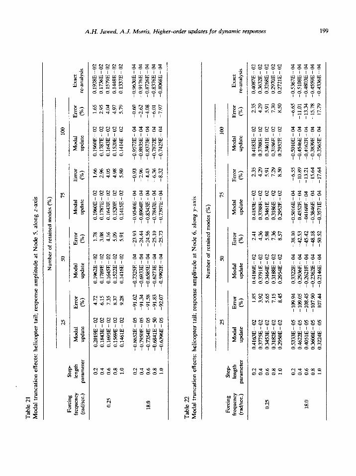
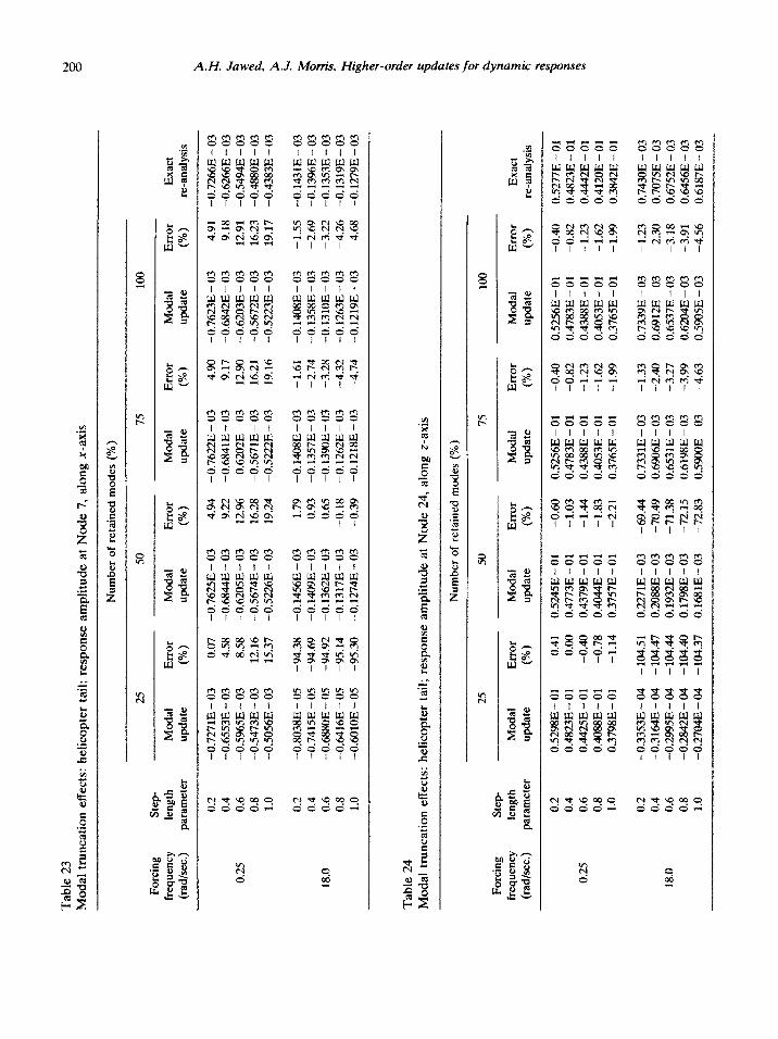
number of significant natural modes retained for the analyses. The natural undamped circular frequencies of the discretized structures range between 0.388 to 70.0 rad/sec. Results for the response amplitudes along selected nodal directions (representing typical design constraints at which the dynamic response needs to be maintained below specified levels), for increasing excitation frequencies, and increasing number of retained modes are set out in Tables 16-24.
Table 6 Planar lo-bar truss nodal data
Nodal coordinates (in.) Disp. boundary conditions”
Node No. X Y X Y
1 720 360 0 0 2 720 0 0 0 3 360 360 1 1 4 360 0 1 1 5 0 360 1 1 6 0 0 1 1
“0, fixed; 1 free,
188 A.H. Jawed, A.J. Morris, Higher-order updates for dynamic responses
Elastic Modulus = 75.OE3 Poisson’s Rati6 = 0.3 Material Density = 0.0025
Fig. 3. Helicopter tail model.
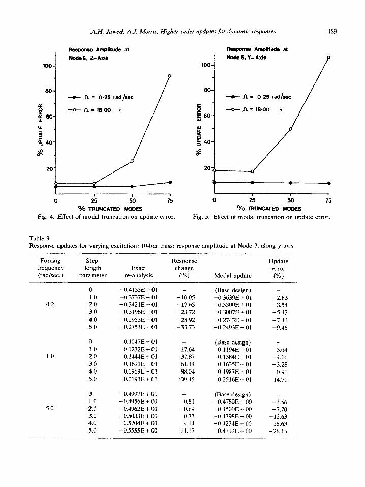
The results (see Figs. 4-7) for increasing excitations are based on full modal matrix, and suggest that provided suthcient higher eigenmodes are included, the update formulation is generally insensitive to frequency variations, and shouid give acceptable results over a wide frequency range. For low excitations (around the fundamental natural frequency), the accuracy is not significantly improved by including higher modes. However, tests show that for
Table 8 Planar IO-bar truss: element data
Nodal Element No. connection
Initial Direction area vector (in.‘) (in.‘)
Table 7 Planar lO-bar truss: loading data
No. of loaded nodes Node No.
Load amplitude
X-camp. Y-camp.
2 4 - 100.00 0 6 - 100.00 0
1 l-3 2 3-5 3 1-4 4 2-3 5 3-4 6 3-6 7 4-S 8 5-6 9 2-4
10 4-6
5.0 0.60 -0.75
0.20 0.20
-0.75 0.15 0.15
-0.75 ” 0.60
5.0 -0.75
loo
80
$ W t g40 8
; 20
A.H. Jawed, A.J. Morris, Higher-order updates for dynamic responses
l3mmmse Amplitude at
Node 6, V- Axis
Reqxme Amplitude at
Nodes, Z-Axis
+n= 0.25 radfsec /
+ A = 1840 *
i
189
0 25 50 75
% TRUNCATED MDDE6
Fig. 4. Effect of modal truncation on update error.
0 25 50 75
% TRUNCATED MODES
Fig. 5. Effect of modal truncation on update error.
Table 9 Response updates for varying excitation: IO-bar truss; response amplitude at Node 3. along y-axis
Forcing frequency (rad/sec.)
Step- length
parameter Exact
re-analysis
Response change
(%) Modal update
Update error
W)
0
1.0
0.2 2.0 3.0
4.0 5.0
1.0
5.0
0 1.0 2.0 3.0 4.0
5.0
0 1.0
2.0 3.0 4.0 5.0
-0.4155E + 01 -
-0.37378 + 01 - 10.05 -0.34218 + 01 - 17.65 -0.31968 + 01 -23.72 -0.29538 + 01 -28.92 -0.2753E + 01 -33.73
0.1047E-k01 - (Base design) 0.12328 + 01 17.64 0.1194E + 01 O.l4#E+Ol 37.87 0.13848 + 01 0.1691E t 01 61.44 0.1635E + 01 0.19698 t 01 88.04 0.1987E + 01 0.2193E + 01 109.45 0.25168 + 01
-0.4997E + 00 - (Base design) -0.4956E + 00 -0.81 -0.47808 i- 00 -0.49628 + 00 -0.69 -0.4500E f 00 -0.50338 t 00 0.73 -0.4398E + 00 -0.5204E t 00 4.14 -0.4234E + 00 -0.5555E + 00 11.17 -0.4102E + 00
(Base design) -
-0.3639E + 01 -2.63 -0.33OOE + 01 -3.54 -0.3007E f 01 -5.13 -0.2743E + 01 -7.11 -0.2493E + 01 -9.46
-3.04 -4.16 -3.28
0.91
14.71
-3.56 -7.70
- 12.63 - 18.63 -26.15
190 A.H. Jawed. A.J. Morris. Higher-order updates for dynamic responses
Table 10
Response updates for varying excitation: lb-bar truss: respond amplitude at Node 4, along p-axis
Forcing Step- frequency length (radlsec.) parameter
Exact re-analysis
Response change
@) Modal update
Update error
(%)
0 -0.4183E + 01 - (Base design) -
1.0 -0.38858 -t 01 -7.14 -0.3922E f 01 0.96
0.2 2.0 -0.359OE f 01 -14.19 -0.3618E + 01 0.79
3.0 -0.3345E f 01 -20.04 -0.3372E + 01 0.79
4.0 -0.315OE -t 01 -24.70 -0.31758 f 01 0.79
5.0 -0.3016E c 01 -27.90 -0.3028E + 01 0.39
0 0.7427E + 00 - (Base design) -
1.0 0.88848 + 00 19.62 0.8645E + 00 -2.59 1.0 2.0 0.10&E + 01 40.74 0.1017E + 01 -2.66
3.0 0.1209E i- 01 62.81 0.1214E + 01 0.39
4.0 0.1346E + 01 81.22 0.1481E + 01 10.00
5.0 0.12568 + 01 69.15 O.l865E+oI 48.42
0 0.57418 + 00 - (Base design) -
1.0 0.5679E f 00 -1.08 O.S559E + 00 -2.12 5.0 2.0 0.564.5E c 00 -1.67 05394E + 00 -4.44
3.0 0.6543E + 00 -1.70 0.5242E + 00 -7.10
4.0 0.5678E + 00 -1.10 05097E + 00 - 10.22 5.0 0.5737E f 00 -0.07 0.4943E i- 00 - 13.83
Forcing frequency
(rad/sec.)
0.2
1.0
5.0
Table 11 Response updates for varying excitation: lo-bar truss; response ampiitude at Node 5, along y-axis
Step- length
parameter
0 1.0 2.0 3.0 4.0 5.0
0
1.0 2.0 3.0 4.0 5.0
0 1.0 2.0 3.0 4.0 5.0
Exact re-analysis
-0.9322E + 01 -0.8483E + 01 -0.7872E + 01 -0.7427E + 01 -0.7168E + 01 -0.72238 + 01
0.2647E + 01
0.2948E -t 01 0.3332E + 01 0.3839E + 01 0.45358 + 01 0.5547E t 0 1
-0.1538E + 01 -0.1435E t 01 -0.136OE t 01 -tl.l305E+Ol -0.1267E + 01 -0.1239E + 01
Response change
W)
- -9.00
- 15.56 -20.33 -23.11 -22.52
-
11.35 25.89 45.04 71.31
109.56
- -6.69
-11.59 -15.13 - 17.60 - 19.44
Modal update
(Base design) -0.82738 + 01 -0.7517E + 01 -0.6874E c 01 -0.6314E f 01 -0.5813E + 01
(Base design)
0.2954E + 01 0.3348E i 01 0.3873E + 01 0.4603E + 01 0.5688E + 01
(Base design) -0.1482E f 01 -O.l427E+Ol -0.13728 + 01 -O.I316E+ 01 -0.12578 f 01
Update error
W)
-2.48 -4.50 -7.44
-11.91 - 19.53
-
0.22 0.48 0.87 1.50 2.53
3.24 4.91 5.11 3.86 1.42
A.H. Jawed, A.J. Morris, Higher-order updates for dynamic responses 191
Table 12 Response updates for varying excitation: IO-bar truss; response amplitude at Node 6, along y-axis
Forcing frequency
(radfsec.)
0.2
Step- length
parameter
0 1.0 2.0 3.0 4.0 5.0
Exact
re-analysis
-0.9328E + 01 -08437E + 01 -0.7822E + 01 -0.7404E + 01 -0.7231E + 01 -0.7567E + 01
Response change
&)
- -9.55
-16.15 -20.63 -22.49 -18.88
Modal update
(Base design) -08592E + 01 -0.7873E + 01 -0.7277E + 01 -0.6781E + 01 -0.6373E + 01
Update error
W)
1.83 0.65
-1.72 -6.21
- 15.77
1.0
0 0.2339E + 01 - (Base design) 1.0 0.2593E + 01 10.85 0.2616E + 01 0.92 2.0 0.29llE + 01 24.46 0.2974E + 01 2.16 3.0 0.3314E + 01 41.71 0.3449E + 01 4.09 4.0 0.3820E + 01 63.33 0.4114E + 01 7.69 5.0 0.4352E + 01 86.09 0.5104E + 01 17.29
5.0
0 0.1695E + 01 - (Base design) 1.0 0.1612E + 01 -4.90 0.1652E + 01 2.52 2.0 0.1562E + 01 -7.81 0.1614E + 01 3.29 3.0 0.1544E + 01 -8.86 0.1580E + 01 2.32 4.0 0.1563E + 01 -7.80 0.1553E + 01 -0.64 5.0 0.1635E + 01 -3.54 0.1533E + 01 -6.20
Table 13 69-element helicopter tail structure; nodal data
Node No.
Nodal co-ordinates Nodal co-ordinates Node
X Y Z No. X Y Z
1” 0.00 400.00 800.00 13 2000.00 125.00 800.00 2” 0.00 -500.00 0.00 14 2000.00 - 125.00 800.00 3” 0.00 500.00 0.00 15 2000.00 125.00 550.00 4” 0.00 -500.00 0.00 16 2~0.00 - 125.00 550.00 5 400.00 350.00 800.00 17 2600.00 106.25 800.00 6 400.00 -350.00 800.00 18 2600.00 - 106.25 800.00
7 400.00 450.00 0.00 19 2800.00 100.00 600.00 8 400.00 -450.00 0.00 20 2800.00 - 100.00 600.00 9 1200.00 150.00 800.00 21 3000.00 56.25 1400.00
10 1200.00 -150.00 ~*# 22 3900.00 -56.25 1400.00 11 1200.00 150.00 500.00 23 3200.00 50.00 1400.00 12 1200.00 - 150.00 500.00 24 3200.00 -50.00 1400.00
’ Restrained nodes.
192 A.H. Jawed, A.J. Morris, Higher-order updates for dynamic responses
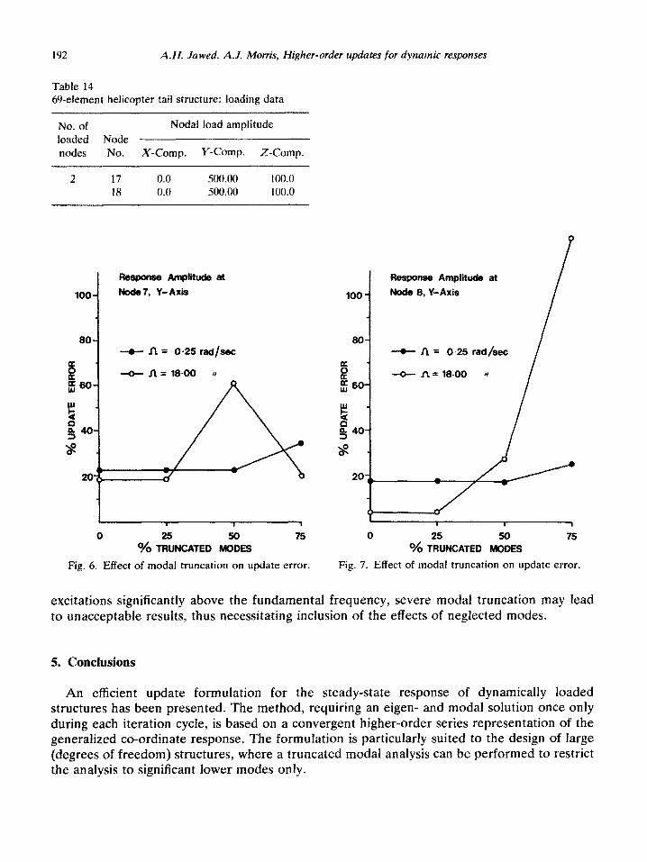
Table 14 69-element helicopter tail structure: loading data
No. of Nodal load amplitude
loaded Node nodes No. X-Comp. Y-Camp. Z-Comp.
2 17 0.0 500.00 100.0 1x 0.0 500.00 100.0
Fig.
bsponrre Amp- Node7, Y-Axis
et
+n= 0.25 radjsac
-o- n = 18.00 II
0 80 % TfkJCATED MODES
75
6. Effect of modal truncation on update error.
100
80
8
; 60
Responss Arnp~~
Node 8, Y-Axis
at
--e-n= 0.25 rad/sec
-@- n = 18.00 N
0 50 O/o TklCATED MODES
75
Fig. 7. Effect of modal truncation on update error.
excitations significantly above the fundamental frequency, severe modal truncation may lead to unacceptable results, thus necessitating inclusion of the effects of neglected modes.
5. Concbions
An efficient update formulation for the steady-state response of dynamically loaded structures has been presented. The method, requiring an eigen- and modal solution once only during each iteration cycle, is based on a convergent higher-order series representation of the generalized co-ordinate response. The formulation is particularly suited to the design of large (degrees of freedom) structures, where a truncated modal analysis can be performed to restrict the analysis to signi~cant lower modes only.
A.H. Jawed, A.J. Morris, Higher-order updates for dynamic responses
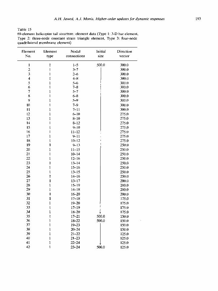
Table 15 69-element helicopter tail structure: element data (Type 1: 3-D bar element, Type 2: three-node constant strain triangle element, Type 3: four-node quadrilateral membrane element)
Element Element No. type
Nodal connections
Initial size
Direction vector
1 1 l-5 2 1 3-7 3 1 2-6 4 1 4-8 5 1 5-6 6 1 7-8 7 1 5-7 8 1 6-8 9 1 5-9
10 1 7-9 11 1 7-11 12 1 6-10 13 1 8-10 14 1 s-12 15 1 9-10 16 1 11-12 17 1 9-11 18 1 lo-12 19 1 9-13 20 1 11-15 21 1 lo-14 22 1 12-16 23 1 13-14 24 1 15-16 25 1 13-15 26 1 14-16 27 1 13-17 28 1 1519 29 1 14-18 30 1 16-20 31 1 17-18 32 1 19-20 33 1 17-19 34 1 18-20 35 1 17-21 36 1 18-22 37 1 19-23 38 1 20-24 39 1 21-22 40 1 21-23 41 1 22-24 42 1 23-24
500.0
V 500.0 500.0
I 500.0
300.0 300.0 300.0 300.0 300.0 300.0 300.0 300.0 300.0
300.0 300.0 275.0 275.0 275.0 275.0 275.0 275.0 275.0 250.0 250.0 250.0 250.0 250.0 250.0 250.0 250.0 200.0 200.0 200.0 200.0 175.0 175.0 175.0 175.0 150.0 150.0 150.0 150.0 125.0 125.0 125.0 125.0
194 A.H. Jawed, A.J. Morris, Higher-order updates for dynamic responses
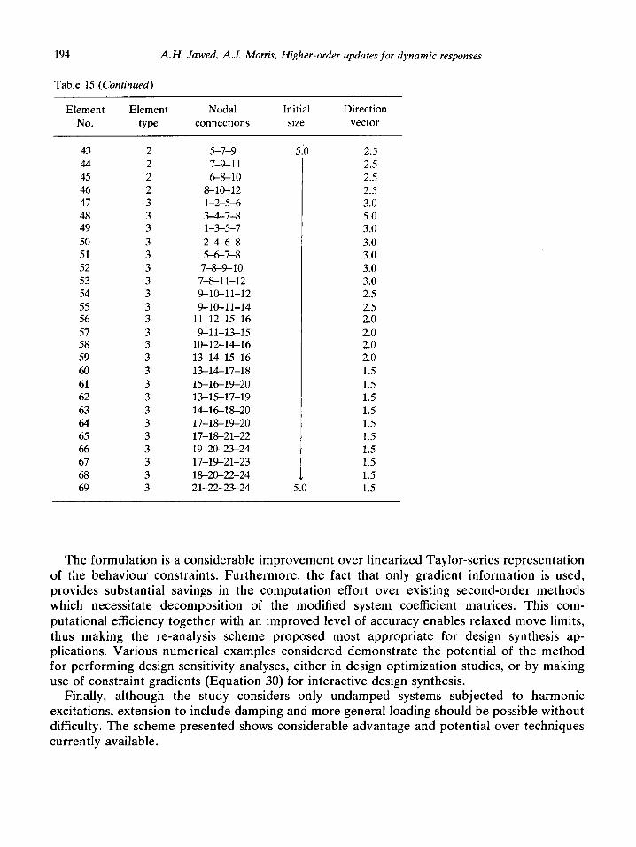
Table 15 (Continued)
Element Element Nodal Initial Direction
No. type connections size vector
43 2 5-7-9 5.b 2.5 44 2 7-9-l 1 2.5 45 2 6-8-10 2.5 46 2 8-10-12 2.5 47 3 l-2-5-6 3.0 48 3 3-4-7-8 5.0 49 3 l-3-5-7 3.0 50 3 2-4-6-8 3.0 51 3 5-6-7-8 3.0 52 3 7-8-9-10 3.0 53 3 7-8-l 1-12 3.0 54 3 9-10-l 1-12 2.5 55 3 9-10-11-14 2.5 56 3 11-12-15-16 2.0 57 3 9-11-13-15 2.0 58 3 10-12-14-16 2.0 59 3 13-14-15-16 2.0 60 3 13-14-17-18 1.5 61 3 15-16-W-20 1.5 62 3 13-15-17-19 1.5 63 3 14-16-18-20 1.5 64 3 17-H-19-20 1.5 65 3 17-18-21-22 1.5 66 3 1%20-23-24 1.5 67 3 17-19-21-23 1.5 68 3 M-20-22-24 1.5 69 3 21-22-23-24 5.0 1.5
The formulation is a considerable improvement over linearized Taylor-series representation of the behaviour constraints. Furthermore, the fact that only gradient information is used, provides substantial savings in the computation effort over existing second-order methods which necessitate decomposition of the modified system coefficient matrices. This com- putational efficiency together with an improved level of accuracy enables relaxed move limits, thus making the re-analysis scheme proposed most appropriate for design synthesis ap- plications. Various numerical examples considered demonstrate the potential of the method for performing design sensitivity analyses, either in design optimization studies, or by making use of constraint gradients (Equation 30) for interactive design synthesis.
Finally, although the study considers only undamped systems subjected to harmonic excitations, extension to include damping and more general loading should be possible without difficulty. The scheme presented shows considerable advantage and potential over techniques currently available.
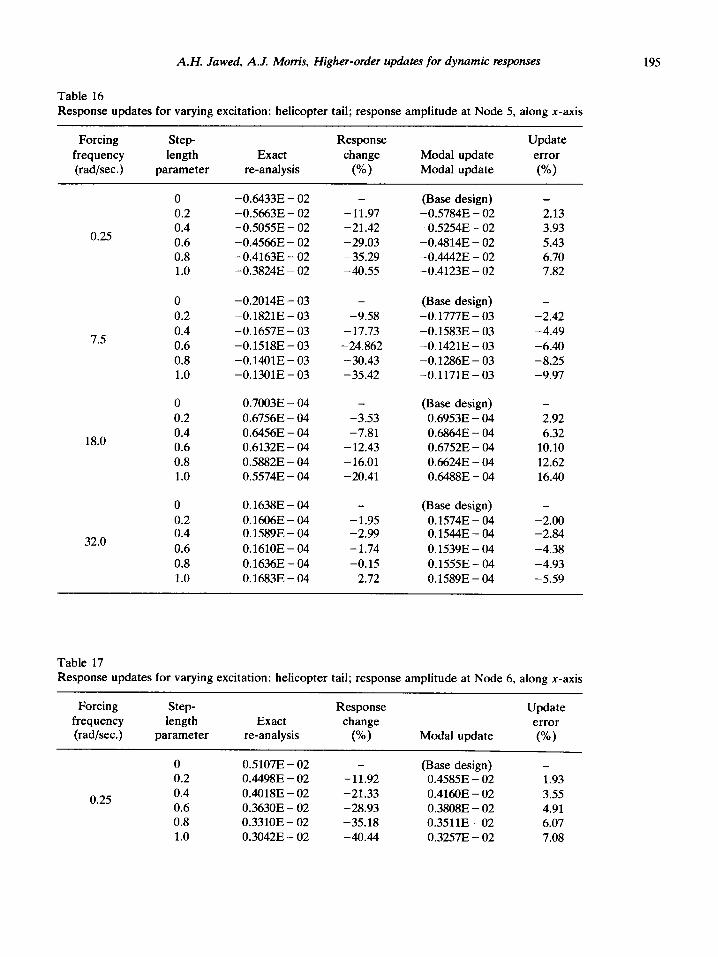
A.H. Jawed, A.J. Mom’s, Higher-order updates for dynamic responses 195
Table 16 Response updates for varying excitation: helicopter tail; response amplitude at Node 5, along x-axis
Forcing frequency (rad/sec.)
Step- length
parameter Exact
re-analysis
Response change
W)
Modal update Modal update
Update error
(%)
0 0.2
-06433E - 02 -0.5663E - 02 -0.5055E - 02 -0.4566E - 02 -0.4163E - 02 -0.38248 - 02
-11.97 -21.42 -29.03 -35.29 -40.55
(Base design) -0.5784E - 02 -0.52548 - 02 -04814E - 02 -0.4442E - 02 -0.4123E - 02
2.13 3.93 5.43 6.70 7.82
0.25 0.4 0.6 0.8 1.0
0 -0.2014E - 03 0.2 -0.1821E - 03 0.4 -0.1657E - 03 0.6 -0.1518E - 03 0.8 -0.14OlE - 03 1.0 -0.1301E - 03
- (Base design) -9.58 -0.1777E - 03
- 17.73 -0.1583E - 03 -24.862 -O.l421E-03 -30.43 -0.1286E - 03 -35.42 -O.l171E-03
-
-2.42 -4.49 -6.40 -8.25 -9.97
7.5
0 0.7003E - 04 0.2 0.6756E - 04 0.4 06456E - 04 0.6 0.6132E - 04 0.8 0.5882E - 04 1.0 0.5574E - 04
(Base design) -
0.69538 - 04 2.92 06864E - 04 6.32 0.6752E - 04 10.10 06624E - 04 12.62 06488E - 04 16.40
-3.53 -7.81
- 12.43 - 16.01 -20.41
18.0
0 0.1638E - 04 0.2 0.1606E - 04 0.4 0.1589E - 04 0.6 0.1610E - 04 0.8 0.1636E - 04 1.0 0.1683E - 04
(Base design) 0.1574E - 04 0.1544E - 04
0.1539E - 04 0.1555E - 04 0.1589E - 04
-1.95 -2.99 -1.74 -0.15
2.72
-2.00 -2.84 -4.38 -4.93 -5.59
32.0
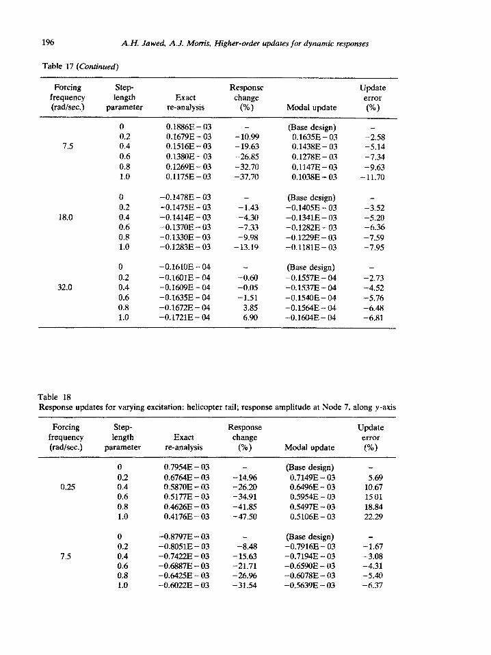
Table 17 Response updates for varying excitation: helicopter tail; response amplitude at Node 6, along x-axis
Forcing frequency (rad/sec.)
Step- length
parameter Modal update
Update error
(%)
Exact re-analysis
Response change
(“h)
0.5107E - 02 -
0.4498E - 02 -11.92 04018E - 02 -21.33 0.3630E - 02 -28.93 0.3310E - 02 -35.18 0.3042E - 02 -40.44
0 0.2
(Base design) -
0.4585E - 02 1.93 0.416OE - 02 3.55 0.3808E - 02 4.91 0.3511E - 02 6.07 0.3257E - 02 7.08
0.25 0.4 0.6 0.8 1.0
196 A.H. Jawed, A.J. Morris, Higher-order updates for dynamic responses
Table 17 (Continued)
Forcing Step- frequency length (radlsec.) parameter
Exact re-analysis
Response change
(%) Modal update
Update error
W)
0 0.18868 - 03 0.2 0.1679E - 03
7.5 0.4 0.1516E - 03 0.6 0.13SOE - 03 0.8 0.1269E - 03 1.0 0.1175E - 03
- 10.99 - 19.63 -26.85 -32.70 -37.70
(Base design) 0.1635E - 03 0.14388 - 03 0.1278E - 03 O.l147E- 03 0.1038E - 03
-2.58 -5.14 -7.34 -9.63
-11.70
18.0
0 -0.1478E - 03 0.2 -0.1475E - 03 0.4 -0.1414E - 03 0.6 -0.137OE - 03 0.8 -0.133OE - 03 1.0 -0.1283E - 03
0 -0.161OE - 04 0.2 -O.l6OlE-04
32.0 0.4 -0.1609E - 04 0.6 -0.16358 - 04 0.8 -0.1672E - 04 1.0 -0.1721E - 04
-1.43 -4.30 -7.33 -9.98
-13.19
-0.60 -0.05 -1.51
3.85 6.90
(Base design) -0.1405E - 03 -0.1341E - 03 -0.1282E - 03 -O.l229E-03 -0.1181E - 03
(Base design) -
-0.1557E - 04 -2.73 -0.1537E - 04 -4.52 -0.1.54OE - 04 -5.76 -0.1564E - 04 -6.48 -0.1604E - 04 -6.81
-3.52 -5.20 -6.36 -7.59 -7.95
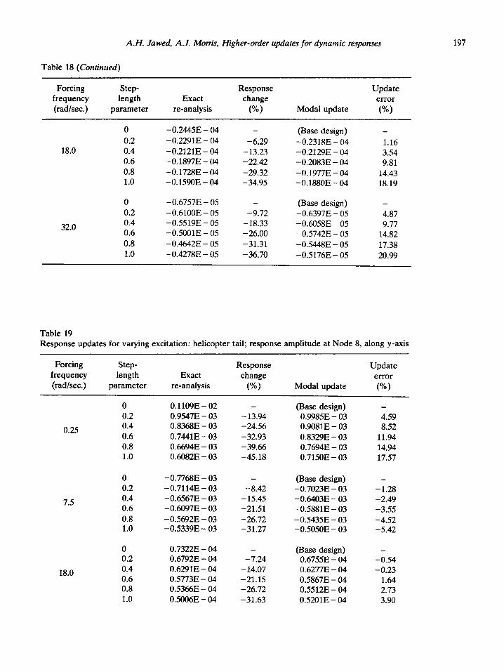
Table 18 Response updates for varying excitation: helicopter tail; response amplitude at Node 7, along y-axis
Forcing Step- frequency length (radlsec.) parameter
Exact re-analysis
Response change
(%) Modal update
Update error
m)
0.25
0 0.79548 - 03 - (Base design)
0.2 0.6764E - 03 - 14.96 0.7149E - 03 0.4 0.587OE - 03 -26.20 0.64968 - 03 0.6 0.5177E - 03 -34.91 0.59548 - 03 0.8 0.4626E - 03 -41.85 0.54978 - 03 1.0 0.4176E - 03 -47.50 0.5106E - 03
5.69 10.67 15 01 18.84 22.29
7.5
0 -0.8797E - 03 - (Base design) 0.2 -0.8051E - 03 -8.48 -0.7916E - 03 0.4 -0.74228 - 03 - 15.63 -0.7194E - 03 0.6 -06887E - 03 -21.71 -0.65908 - 03 0.8 -0.6425E - 03 -26.96 -0.60788 - 03 1.0 -06022E - 03 -31.54 -0S639E - 03
-1.67 -3.08 -4.31 -5.40 -6.37
A.H. Jawed, A.J. Mom’s, Higher-order updates for dynamic responses 197
Table 18 (Continued)
Forcing frequency (rad/sec.)
Step- length
parameter Exact
re-analysis
Response change
W) Modal update
Update error
W)
18.0
0 -0.2445E - 04 -
0.2 -0.2291E - 04 -6.29 0.4 -0.2121E - 04 -13.23 0.6 -0.1897E - 04 -22.42
0.8 -0.1728E - 04 -29.32 1.0 -0.159OE - 04 -34.95
(Base design) -
-0.2318E - 04 1.16 -0.2129E 04 - 3.54 -0.2083E - 04 9.81 -0.1977E - 04 14.43 -0.1880E - 04 18.19
32.0
0 -0.6757E - 05 - (Base design)
0.2 -0.6100E - 05 -9.72 -0.6397E - 05 4.87
0.4 -0.5519E - 05 - 18.33 -06058E 05 - 9.77 0.6 -0.5001E - 05 -26.00 -0.5742E - 05 14.82
0.8 -0.4642E - 05 -31.31 -0.5448E - 05 17.38
1.0 -0.4278E - 05 -36.70 -0.5176E - 05 20.99
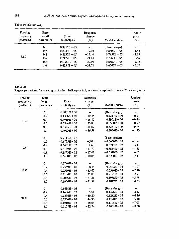
Table 19 Response updates for varying excitation: helicopter tail; response amplitude at Node 8, along y-axis
Forcing frequency (rad/sec.)
Step- length
parameter Exact
re-analysis
Response change
W) Modal update
Update error
(“h)
0.25
0 0.1109E - 02 - (Base design)
0.2 0.9547E - 03 - 13.94 0.9985E - 03 4.59 0.4 0.8368E - 03 -24.56 09081E 03 - 8.52
0.6 0.7441E - 03 -32.93 0.8329E - 03 11.94
0.8 0.6694E - 03 -39.66 0.7694E - 03 14.94 1.0 0.6082E - 03 -45.18 0.7150E - 03 17.57
7.5
18.0
0 -0.7768E - 03 - (Base design)
0.2 -0.7114E - 03 -8.42 -0.7023E - 03 -1.28
0.4 -0.6567E - 03 - 15.45 -06403E - 03 -2.49
0.6 -06097E - 03 -21.51 -0.5881E - 03 -3.55
0.8 -0.5692E - 03 -26.72 -0.5435E - 03 -4.52 1.0 -0.5339E - 03 -31.27 -0.5050E - 03 -5.42
0 0.7322E - 04 - (Base design) 0.2 0.6792E - 04 -7.24 0.6755E - 04 -0.54 0.4 0.6291E - 04 - 14.07 0.6277E - 04 -0.23
0.6 0.5773E - 04 -21.15 0.5867E - 04 1.64 0.8 0.5366E - 04 -26.72 0.5512E - 04 2.73
1.0 0.5006E - 04 -31.63 0.5201E - 04 3.90
A.H. Jawed, A.J. Mortis, Higher-order updates for dynamic responses
Table 19 (Continued)
Forcing Step- frequency length (rad/sec.) parameter
0 0.2
32.0 0.4 0.6
0.8 1.0
Exact re-analysis
0.9856E - 05 08933E - 05
- 0.8135E 05 0.7477E - 0.5
0.6989E - 05 0.6534E - 05
Response change
W)
- -9.36
-17.46 -24.14
-29.09 -33.71
Modal update
(Base design) 0.8804E - 05 0.7957E - 05 0.7263E - 05
0.6687E - 05 0.6203E - 05
Update error
@)
-1.44 -2.19 -2.85
-4.32 -5.07
Table 20 Response updates for varying excitation: helicopter tail; response amplitude at node 21, along y-axis
Forcing frequency (radkec.)
0.25
Step- length
parameter
0 0.2 0.4 0.6 0.8 1.0
7.5
18.0
Exact re-analysis
Response change
(“IO) Modal update
Update error
W)
0.4831E + 00 0.4326E + 00 0.3919E + 00 0.3584E + 00 0.3303E + 00 0.3063E + 00
- 10.45 - 18.86 -25.80 -31.62 -36.58
(Base design) 0.4317E + 00 0.3901E + 00 0.35.58E + 00 0.3271E + 00 0.3026E + 00
-0.21 -0.46 -0.72 -0.98 -1.23
0 -0.7114E- 02 - (Base design) 0.2 -0.6755E - 02 -5.04 -O&DOE - 02 0.4 -06431E - 02 -9.60 -0.6212E - 02 0.6 -0.6139E - 02 - 13.70 -0.5844E - 02 0.8 -0.5873E - 02 - 17.43 -0.5519E - 02 1.0 -0563OE- 02 -20.86 -0.5230E - 02
-1.84 -3.41 -4.80 -6.03 -7.11
0 0.27%E - 03 - (Base design) 0.2 0.2559E - 03 -8.48 0.2532E - 03 0.4 0.2359E - 03 - 15.62 0.2310E - 03 0.6 0.21848 - 03 -21.88 0.2121E - 03 0.8 0.2035E - 03 -27.21 0.1958E - 03 1.0 0.1904E - 03 -31.91 0.1817E - 03
-1.07 -2.10 -2.91 -3.78 -4.55
32.0
0 O.l488E-03 - (Base design) 0.2 0.1406E - 03 -5.51 0.1376E - 03 0.4 0.1336E - 03 - 10.20 0.1282E - 03 0.6 O.l266E-03 - 14.93 0.1198E - 03 0.8 0.121OE - 03 - 18.68 0.1125E - 03 1.0 O.l157E- 03 -22.24 0.1061E - 03
-2.12 -4.16 -5.40 -7.03 -8.30
Tab
le 2
1 M
odal
tru
nca
tion
ef
fect
s:
hel
icop
ter
tail
; re
spon
se
amp
litu
de
at N
ode
5, a
lon
g z-
axis
Nu
mbe
r of
ret
ain
ed
mod
es
(%)
For
cin
g S
tep-
fr
equ
ency
le
ngt
h
(rad
/sec
.)
para
met
er
0.2
0.4
0.25
0.
6 0.
8 1.
0
25
50
75
100
Mod
al
Err
or
Mod
al
Err
or
Mod
al
Err
or
Mod
al
Err
or
Exa
ct
upd
ate
(“h
) u
pdat
e (%
) u
pdat
e (%
I u
pdat
e W
) re
-an
alys
is
0.20
19E
-
02
4.72
O
.l%
2E
- 02
1.
78
0.19
6OE
- 02
1.
66
0.19
6OE
-
02
1.65
0.
1928
E -
02
O
.l&
13E
- 02
6.
15
0.17
89E
-
02
3.08
0.
1787
E -
02
2.
%
0.17
87E
-
02
2.95
0.
1736
E -
02
0.
169S
E -
02
7.
35
0.16
45E
-
02
4.16
0.
1643
E -
02
4.
05
0.16
43E
-
02
4.04
0.
1579
E -
02
0.
1569
E -
02
8.
37
0.15
22E
-
02
5.09
0.
1520
E -
02
4.
98
0.15
2OE
-
02
4.97
0.
1448
E -
02
0.
1461
E -
02
9.
28
0.14
16E
-
02
5.91
0.
1415
E -
02
5.
80
0.14
14E
-
02
5.79
0.
1337
E -
02
0.2
-0.8
6528
-
OS
-9
1.02
-0
.732
SE
04
-2
3.93
-0
.954
OE
-
04
-0.9
3 -0
.957
28
- 04
-0
.60
-O.%
3OE
-
- 04
0.
4 -0
.79S
OE
-
05
-91.
34
-069
33E
04
-2
4.44
-0
.890
4E
04
-2.9
6 -0
.893
SE
-
04
-2.6
2 -0
.917
68
- -
- 04
18
.0
0.6
-0.7
3S4E
-
OS
-9
1.58
-0
.658
SE
-
04
-24.
56
-0.8
343E
-
04
-4.4
3 -0
.837
3E
- 04
-4
.08
-0.8
726E
-
04
0.8
-tL
684l
E-
50
-91.
83
-0.6
273E
-
04
-25.
10
-0.7
843E
-
04
-6.3
6 -0
.787
2E
- 04
-6
.01
-0.8
376E
-
04
1.0
-0.6
3%E
-
OS
-9
2.07
-0
.599
2E
- 04
-2
5.73
-0
.739
7E
- 04
-8
.32
-0.7
42S
E
- 04
-7
.97
-0.8
068E
-
04
Tab
le 2
2 M
odal
tru
nca
tion
ef
fect
s:
hel
icop
ter
tail
; re
spon
se
amp
litu
de
at N
ode
6, a
lon
g y-
axis
Nu
mb
er o
f re
tain
ed m
odes
(%
)
For
cin
g S
tep
freq
uen
cy
len
gth
(r
ad/s
ec.)
pa
ram
eter
0.2
0.4
0.25
0.
6 0.
8 1.
0
25
Mod
al
upd
ate
0.41
63E
-
02
0.37
7SE
-
02
0.34
.53E
- 02
0.
3182
E-0
2 0.
29S
OE
- 02
Err
or
fi) 1.
85
3.92
5.
65
7.1s
8.
45
50
75
100
Mod
al
Err
or
Mod
al
Err
or
Mod
af
Err
or
Exa
ct
upd
ate
(%I
upd
ate
(%I
upd
ate
(“/I
re
-an
alys
is
0.41
86E
-
02
2.41
0.
4183
E -
02
2.
35
0.41
83E
-
02
2.35
0.
4087
8 -
02
0.37
918
- 02
4.
36
0.37
88E
-
02
4.29
0.
3788
E -
02
4.
29
0.36
32E
-
02
0.34
64E
-
02
5.98
0.
3461
E -
02
5.
91
0.34
61E
-
02
5.91
0.
3268
E -
02
0.
3188
E -
02
7.
36
0.31
86E
-
02
7.29
0.
3186
E -
02
7.
30
0.29
70E
-
02
0.29
S4E
-
02
8.57
0.
2952
E -
02
&
SO
0.
2952
E -
02
8.
50
0.27
2lE
-
02
0.2
0533
3E
- 05
-1
99.9
4 -0
.332
2E
- 04
-3
8.10
-0
SO
16E
-
04
-6.5
5 -O
.SO
lOE
-
04
-6.6
5 -0
5367
E
- 04
0.
4 0.
4622
E -
O
S
- 10
9.05
-0
.293
6E
- 04
-4
2.53
-0
.455
2E
- 04
-
10.8
9 -0
.454
6E-0
4 -1
1.01
-0
5108
E-0
4 18
.0
0.6
0.4O
SlE
- 0
5 -1
08.4
5 -0
.262
1E-
04
-45.
42
-041
68E
-
04
-13.
21
-0.4
162E
-
04
- 13
.34
-0.4
8038
-
04
0.8
0.36
OO
E -
OS
-1
07.9
0 -0
.236
2E
- 04
-4
8.18
-0
.384
6E-
04
-15.
64
-0.3
8398
-
04
-15.
78
-0.4
5598
-
04
1.0
0.32
248
- 05
-
107.
44
-0.2
146E
-
04
-50.
52
-0.3
571E
-
04
-17.
64
-0.3
56S
E
- 04
-
17.7
9 -0
.433
6E
- 04
Tab
le
23
Mod
al
trun
catio
n ef
fect
s:
helic
opte
r ta
il;
resp
onse
am
plit
ude
at
Nod
e 7,
at
ong
x-ax
is
Nu
mbe
r of
ret
ain
ed m
odes
(%
}
For
cin
g S
tep-
fr
equ
ency
le
ngt
h
(rad
/sec
.)
para
met
er
25
50
75
100
Mod
al
Err
or
Mod
al
Err
or
Mod
al
Err
or
Mod
al
Err
or
Exa
ct
upd
ate
&)
upd
ate
(%)
upd
ate
W)
upd
ate
(%)
re-a
nal
ysis
0.2
-0.7
271E
-
03
0.07
-0
.762
SE
-
03
4.94
-0
.762
2E
- 03
4.
90
-0.7
623E
-
03
4.91
-0
.726
6E
- 03
0.4
-0.6
5531
;: -
03
4.58
-O
&W
E-0
3 9.
22
-068
41E
-
03
9.17
-0
6842
E
- 03
9.
18
-0.6
266E
-
03
0.25
0.
6 -0
.5%
5E
- 03
8.
58
-0.6
205E
-
03
12.%
-0
.620
2E
- 03
12
.90
-0.6
2D3E
-
03
12.9
1 -0
S49
4E
- 03
0.8
-0S
473E
-
03
12.1
6 -0
.S67
4E
- 03
16
.28
-0.5
671E
-
03
16.2
1 -0
.567
2E
- 03
16
.23
-O&
BO
B
- 03
1.0
-0S
OS
6E
- 03
15
.37
-0.5
2268
-
03
19.2
4 -0
.522
2E
- 03
19
.16
-0.5
223E
-
03
19.1
7 -0
.438
3E
- 03
0.2
-0.8
038E
- 05
-9
4.38
-0
.145
6E
- 03
1.
79
-0.1
408E
-
03
-1.6
1 -0
.140
8E
- 03
-1
.55
-O.l
431E
- 03
0.4
-0.7
4158
-
05
-94.
69
-0.1
499E
-
03
0.93
-0
.135
7E
- 03
-2
.74
-0.1
358E
-
03
-2.6
9 -O
.l3%
E-
03
18.0
0.
6 -0
688O
E
- 05
-9
4.92
-0
.136
2E
- 03
0.
65
-0.1
39O
E
- 03
-3
.28
-0.1
310E
- 03
-3
.22
-0.1
3538
- 03
0.8
-064
16E
-05
-95.
14
-O.l
317E
-03
-0.1
8 -0
.126
2E
- 03
-4
.32
-0.1
263E
-
03
-4.2
6 -0
.131
9E
- 03
1.0
-0.6
OlO
E
- 05
-9
5.30
-0
.127
4E
- 03
-0
.39
-0.1
218E
-
03
-4.7
4 -0
.121
9E
- 03
-4
.68
-O.l
279E
- 03
Tab
le
24
Mod
al
trun
catio
n ef
fect
s:
helic
opte
r ta
il;
resp
onse
am
plitu
de
at N
ode
24,
alon
g z-
axis
Nu
mbe
r of
ret
ain
ed m
odes
(%
)
For
cin
g S
tep-
fr
equ
ency
le
ngt
h
(rad
lsec
.)
para
met
er
0.2
0.4
0.25
0.
6 0.
8 1.
0
25
so
75
100
Mod
al
Err
or
Mod
al
Err
or
Mod
al
Err
or
Mod
al
Err
or
Exa
ct
upd
ate
(“/)
u
pdat
e (“
/)
upd
ate
1%)
upd
ate
W)
re-a
nai
ysis
0.52
98E
-
01
0.41
0.
5245
E -
01
-0
.60
0.52
56E
-
01
-0.4
0 O
.S2S
6E -
01
-0.4
0 O
S27
7E -
01
0.48
23E
-
01
0.00
0.
4773
E -
01
-1
.03
0.47
83E
-
01
-0.8
2 0.
4783
E -
01
-0
.82
0.48
23E
-
01
0.44
258
- 01
-0
.40
0.43
798
- 01
-1
.44
0.43
88E
-
01
-1.2
3 0.
4388
E -
01
-1
.23
0.44
42E
-
01
0.40
8gE
-
01
-0.7
8 0.
4044
E -
01
-1
.83
0.40
53E
-
01
-1.6
2 0.
4053
E -
01
-1
.62
0.41
2QE
- 0
1
0.37
98E
-
01
-1.1
4 0.
3757
E-0
1 -2
.21
0.37
65E
-
01
-1.9
9 0.
376S
E -
01
-1
.99
0.38
42E
-
01
0.2
-0.3
353E
-
04
- 10
4.51
0.
2271
E -
03
-6
9.44
0.
7331
E -
03
-1
.33
0.73
39E
-
03
-1.2
3 0.
743O
E -
03
0.4
-0.3
164E
-
04
-104
.47
0.20
88E
-
03
-70.
49
0.69
06E
- 0
3 -2
.40
0.69
12E
-
03
-2.3
0 0.
7075
E -
03
18.0
0.
6 -0
.299
58
- 04
-1
04.4
4 0.
1932
E -
03
-7
1.38
0.
6531
E -
03
-3
.27
0.65
37E
- 0
3 -3
.18
0.67
528
- 03
0.8
-0B
42E
-
04
-104
.40
0.17
98E
-
03
-72.
15
0.61
98E
-
03
-3.9
9 0.
6204
E -
03
-3
.91
0.64
S6E
- 0
3
1.0
-OX
WE
-04
-104
.37
O.l
681E
- 03
-7
2.83
0.
59O
OE
- 03
-4
.63
0590
5E
- 03
-4
.56
0.61
878
- 03
A.H. Jawed, A.J. Morris, Higher-order updates for dynamic responses 201
References
[l] L. Meirovitch, Computational Methods in Structural Dynamics (Sijthoff and Noordhoff, Alpen a/d Rijn, 1980). [2] G. Ryland and L. Meirovitch, Response of vibrating systems and perturbed parameters, J. Guidance and
Control 3(4) (1980) 298-303. [3] K.O. Kim, W.J. Anderson and R.E. Sandstrom, Non-linear inverse perturbation method in dynamic analysis,
AIAA J. 21(9) (1983) 1310-1316. [4] E.J. Haug and B. Rousselet, Design sensitivity analysis in structural mechanics II. Eigenvalue variations, J.
Struct. Mech. 8(2) (1980) 161-186. [5] H. Miura and L. Schmit, Second order approximation of natural frequency constraints in structural synthesis,
Internat. J. Numer. Meths. Engrg. 13 (1978) 337-351. [6] A.J. Morris, ed., Foundations of Structural Optimization -A Unified Approach (Wiley, New York, 1982). 171 L. Kitis, B.P. Wang and W.D. Pilkey, Vibration reduction over a frequency range, J. Sound Vibration 89(4)
(1983) 559-569. [8] A.H. Jawed and A.J. Morris, Approximate higher-order sensitivities in structural design, Engrg. Optimization
7(2) (1984) 121-142.
Related Documents