Higher Order SM Block-Control of Nonlinear Systems with Unmodeled Actuators: Application to Electric Power Systems and Electrohydraulic Servo-Drives

Higher Order SM Block-Control of NonlinearSystems with Unmodeled Actuators: Applicationto Electric Power Systems and ElectrohydraulicServo-Drives

Alexander G. Loukianov1, Leonid Fridman2, Jose M. Canedo1,Edgar Sanchez1, and Adolfo Soto-Cota3

1 Centro de Investigacion y de Estudios Avanzados del IPN,A. P. 31-438,C.P. 44550, Guadalajara, Jal., [email protected]

2 Universidad Nacional Autonoma de Mexico,Facultad de Ingenierıa, Ciuadad Univercitaria, [email protected]

3 Instituto Tecnologico de Sonora, 5 de Febrero 818 sur, Cd. Obregon, Sonora Mexico

1 Introduction

The dynamics of the most of the industrial plants (for example electric powersystem, electromechanical system, electro-hydraulic system and so on) are highlynonlinear and, moreover, include actuator dynamics which increase the relativedegree of the complete system. To stabilize the plant dynamics it is naturally toapplied some feedback linearization (FL) technique: block control [18], backstep-ping [14] or input-output linearization [11], since the model of these plants can bepresented in the nonlinear block controllable form or (the same) strict-feedbackone. All these control techniques require to calculate the time derivatives of theplant dynamics vector fields (Lie derivatives), results in a computationally ex-pensive control algorithm, and moreover, the closed-loop system is susceptible toplant parameter variations and disturbances. To simplify the control algorithmthe actuator fast dynamics are usually skipped, and to overcome the robustproblem the sliding mode (SM) control [25] in combination with FL technique[18], [17] can be can be applied. However, the presence of the actuator unmod-eled fast dynamics can destroy the desired behavior of the SM control systemscausing lost of robustness and accuracy and provoking the chattering effect [25],[8]. Therefore, the problem of control design for the systems with unmodeledactuator dynamics becomes to be a big challenge.

This chapter proposes the control scheme based on the combination of theblock control and SM control techniques. For this propose, the chapter is orga-nized as follows. In Section 2, a class of nonlinear minimum phase SISO systemspresented in nonlinear block controllable form (NBC form), that models boththe plant and actuator dynamics, is presented. In subsection 2.1, consideringthe complete plant and actuator dynamics, the block control technique is first

G. Bartolini et al. (Eds.): Modern Sliding Mode Control Theory, LNCIS 375, pp. 401–425, 2008.springerlink.com c© Springer-Verlag Berlin Heidelberg 2008

402 A.G. Loukianov et al.

used to design a nonlinear sliding manifold for achieving the error tracking, andthen the First Order Sliding Mode (FOSM) [25] algorithm is implemented toensure finite time convergence of the state vector to the designed SM manifold.In subsection 2.2, a less dimension sliding manifold is designed based on theplant dynamics only, then High Order Sliding Mode (HOSM) algorithm [15] isimplemented to achieve chattering free motion of the closed-loop system in pres-ence of the actuator unmodeled dynamics. Finally, a robust exact differentiator[15] is used to obtain the estimates of the sliding variable and its derivatives.In Section 3, the proposed method is applied to design robust controller for apower electric system in presence of the exciter system unmodeled fast dynam-ics [9]. Section 4 deals with neuronal network second order SM block controlfor an electro-hydraulic system in presence of the electric actuator unmodeledfast dynamics [16]. The simulations results show the reasonable behavior of thedesigned controllers. Finally, relevant conclusions are stated in Section 5.

2 The Idea of Nonlinear Block Higher Order SlidingMode Controllers

Consider a class of nonlinear SISO system presented (possibly after a nonlineartransformation) in the NBC form consisting of r blocks [18] (or strict feedbackform [14]) subject to uncertainties

x1 = f1(x1) + b1(x1)x2 + g1(x1, t)xi = fi(xi) + bi(xi)xi+1 + gi(xi, t), i = 2, . . . , r − 1 (1)xr = fr(xr , xr+1) + br(xr , xr+1)u + gr(xr , xr+1, t)

.xr+1 = fr+1(xr, xr+1, t) (2)

y = x1 (3)

where the state vector x ∈ Rn is decomposed as x=(x1, . . . , xr, xr+1, . . . , xn)T =(xr, xr+1)T , xi = (x1, . . . , xi)T , i = 1, . . . , r ; y and u ∈ R; fi(·) and bi(·) areknown sufficiently smooth functions of their arguments, gi(·) is an uncertain butbounded function, and bi(·) �= 0 over the set D1× D2:

D1 = {xr ∈ Rr | ‖xr‖2 ≤ r1, r1 > 0} r1 (4)

D2 ={xr+1 ∈ Rn−r | ‖xr+1‖2 ≤ r2, r2 > 0

}(5)

Suppose

A1) The set‖xr+1‖2 ≤ d0 < r2, d0 > 0. (6)

is uniformly attractive with respect to the set D2 , i.e. for any solution to thesystem

.xr+1 = fr+1(0, xr+1, t) (7)

describing zero dynamics in (1)-(3) with any initial conditions from D2 thereexists T such that for all t > T we will have ‖xr+1(t)‖2 ≤ d0.

Higher Order SM Block-Control of Nonlinear Systems 403

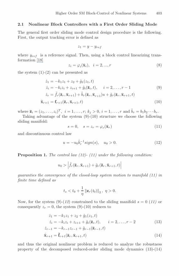
2.1 Nonlinear Block Controllers with a First Order Sliding Mode

The general first order sliding mode control design procedure is the following.First, the output tracking error is defined as

z1 = y − yref

where yref is a reference signal. Then, using a block control linearizing trans-formation [18]

zi = ϕi(xi), i = 2, ..., r (8)

the system (1)-(2) can be presented as

z1 = −k1z1 + z2 + g1(z1, t)zi = −kizi + zi+1 + gi(zi, t), i = 2, . . . , r − 1 (9)

zr = fr(zr , xr+1) + br(zr, xr+1)u + gr(zr , xr+1, t).xr+1 = fr+1(zr, xr+1, t) (10)

where zi = (z1, . . . , zi)T , i = 1, . . . , r; kj > 0, i = 1, . . . , r and br = b1b2 · · · br.Taking advantage of the system (9)-(10) structure we choose the following

sliding manifold:s = 0, s = zr = ϕr(xr) (11)

and discontinuous control law

u = −u0b−1r sign(s), u0 > 0. (12)

Proposition 1. The control law (12)- (11) under the following condition:

u0 >∣∣∣fr(zr, xr+1) + gr(zr, xr+1, t)

∣∣∣

guaranties the convergence of the closed-loop system motion to manifold (11) infinite time defined as

ts < t0 +1η

‖zr(t0)‖2 , η > 0.

Now, for the system (9)-(12) constrained to the sliding manifold s = 0 (11) orconsequently zr = 0, the system (9)-(10) reduces to

z1 = −k1z1 + z2 + g1(z1, t)zi = −kizi + zi+1 + gi(zi, t), i = 2, . . . , r − 2 (13)

zr−1 = −kr−1zr−1 + gr−1(zr−1, t).xr+1 = fr+1(zr , xr+1, t) (14)

and thus the original nonlinear problem is reduced to analyze the robustnessproperty of the decomposed reduced-order sliding mode dynamics (13)-(14)

404 A.G. Loukianov et al.

which can be considered as linear system with nonlinear perturbation, un-matched with respect to the control u in the system (9)-(10).

It is clear that when s = 0, stability of the system (13)-(14) is determined bythe values of the controller gains ki, i=1, ..., r − 1.

Assume

A2) There exist positive constants qij and di such that

|g1(z1, t)| ≤ q11 |z1| + d1

|g2(z2, t)| ≤ k1q21 |z1| + q22 |z2| + d2

|gi(zi, t)| ≤i∑

j=1

k(i−j)j qi,j |zj | + di, i = 3, ..., r − 1, j = 3, ..., i.

To achieve the robustness property with respect to unknown but boundeduncertainty, the controller gains ki, i = 1, ..., r − 1 have to be chosen hierarchi-cally high. Thus, since g1(z1, t) does not depend on k1, the value of this gaincan be chosen such that the term k1z1 in the first block of (13)-(14) will domi-nate. By block linearization procedure, the term g2(z2, t) depends on k1 but notk2,...,kr−1. Then for fixed k1, the appropriate choice of k2 value the term k2z2in the second block of (13)-(14) will be also dominating, and so on. Finally, aconstructive step-by-step Lyapunov technique approach [18] establishes the sta-bility property of the SM motion on zr = 0, and provides the required values ofthe controller gains k1, ..., kr−1. So

Theorem 1. [18]. Let the Assumption A1 and A2 hold. Then there exist posi-tive scalars k1, ..., kr−1 and h1, ..., hr−1 such that a solution of the system (13)-(14) is uniformly ultimately bounded, i.e.

lim supt→∞

|zi(t)| ≤ hi, i = 1, ..., r − 1.

To derive the linearizing transformation (69) it is necessary to calculate the suc-cessive derivatives of fi(xi) and bi(xi), i = 1, . . . , r − 1 in (1)-(2), that resultsin a computationally expensive control algorithm. Moreover, to achieve robust-ness with respect to unmatched perturbations gi(zi, t), i = 1, . . . , r − 1 thecontroller gains k1, ..., kr−1 must be sufficiently high. To overcome these prob-lems the HOSM control combined with a robust exact differentiator [15] will beapplied in the next section.

2.2 Nonlinear Block Controller with Higher Order Sliding Modes

Assume that the system (1)-(3) models both the plant and its actuator with therelative degrees k and q, respectively, so k + q = r. Therefore, choosing s0

s0 = zk+1 = ϕk+1(xk+1) (15)

(8) as a sliding variable, and then taking its successive derivatives, straightfor-ward calculations give

Higher Order SM Block-Control of Nonlinear Systems 405

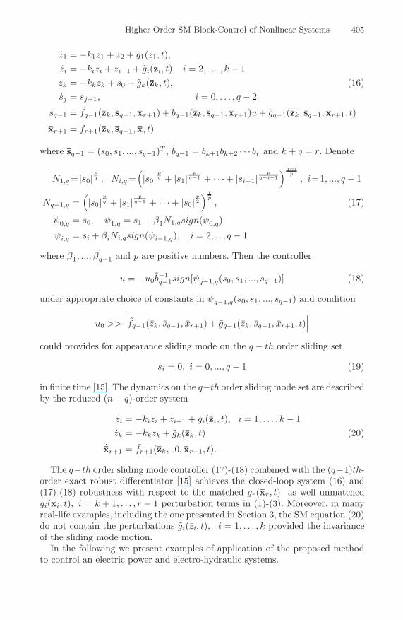
z1 = −k1z1 + z2 + g1(z1, t),zi = −kizi + zi+1 + gi(zi, t), i = 2, . . . , k − 1zk = −kkzk + s0 + gk(zk, t), (16)sj = sj+1, i = 0, . . . , q − 2

sq−1 = fq−1(zk, sq−1, xr+1) + bq−1(zk, sq−1, xr+1)u + gq−1(zk, sq−1, xr+1, t).xr+1 = fr+1(zk, sq−1, x, t)

where sq−1 = (s0, s1, ..., sq−1)T , bq−1 = bk+1bk+2 · · · br and k + q = r. Denote

N1,q = |s0|pq , Ni,q =

(|s0|

pq + |s1|

pq−1 + · · · + |si−1|

pq−i+1

) q−ip

, i=1, ..., q − 1

Nq−1,q =(|s0|

pq + |s1|

pq−1 + · · · + |s0|

p2

) 1p

, (17)

ψ0,q = s0, ψ1,q = s1 + β1N1,qsign(ψ0,q)

ψi,q = si + βiNi,qsign(ψi−1,q), i = 2, ..., q − 1

where β1, ..., βq−1 and p are positive numbers. Then the controller

u = −u0b−1q−1sign[ψq−1,q(s0, s1, ..., sq−1)] (18)

under appropriate choice of constants in ψq−1,q(s0, s1, ..., sq−1) and condition

u0 >>∣∣∣fq−1(zk, sq−1, xr+1) + gq−1(zk, sq−1, xr+1, t)

∣∣∣

could provides for appearance sliding mode on the q − th order sliding set

si = 0, i = 0, ..., q − 1 (19)

in finite time [15]. The dynamics on the q−th order sliding mode set are describedby the reduced (n − q)-order system

zi = −kizi + zi+1 + gi(zi, t), i = 1, . . . , k − 1zk = −kkzk + gk(zk, t) (20)

.xr+1 = fr+1(zk, , 0, xr+1, t).

The q−th order sliding mode controller (17)-(18) combined with the (q−1)th-order exact robust differentiator [15] achieves the closed-loop system (16) and(17)-(18) robustness with respect to the matched gr(xr, t) as well unmatchedgi(xi, t), i = k + 1, . . . , r − 1 perturbation terms in (1)-(3). Moreover, in manyreal-life examples, including the one presented in Section 3, the SM equation (20)do not contain the perturbations gi(zi, t), i = 1, . . . , k provided the invarianceof the sliding mode motion.

In the following we present examples of application of the proposed methodto control an electric power and electro-hydraulic systems.

406 A.G. Loukianov et al.

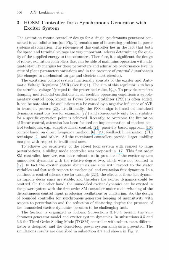
3 HOSM Controller for a Synchronous Generator withExciter System

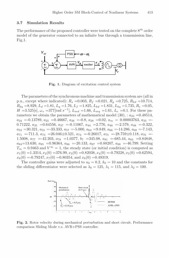
The excitation robust controller design for a single synchronous generator con-nected to an infinite bus (see Fig. 1) remains one of interesting problem in powersystems stabilization. The relevance of this controller lies in the fact that boththe speed and terminal voltage are very important indexes determining the qual-ity of the supplied energy to the consumers. Therefore, it is significant the designof robust excitation controllers that can be able of maintains operation with ade-quate stability margins for these parameters and admissible performance level inspite of plant parameters variations and in the presence of external disturbances(for changes in mechanical torque and electric short circuits).

The excitation control system functionally consists of the exciter and Auto-matic Voltage Regulator (AVR) (see Fig.1). The aim of this regulator is to keepthe terminal voltage VT equal to the prescribed value, Vref . To provide sufficientdamping multi-modal oscillations at all credible operating conditions a supple-mentary control loop, known as Power System Stabilizer (PSS) is often added.It can be note that the oscillations can be caused by a negative influence of AVRin transient process [20]. Traditionally, the PSS design is based on linearizeddynamics equations (see for example, [22]) and consequently only local stabilityfor a specific operation point is achieved. Recently, to overcome the limitationof linear control, attention has been focused on implementation of modern con-trol techniques, e.g., adaptive linear control, [24]; passivity based approach [10];control based on direct Lyapunov method, [6], [20]; feedback linearization (FL)technique [2], and others. All the mentioned controllers provide larger stabilitymargins with respect to traditional ones.

To achieve low sensitivity of the closed loop system with respect to largeperturbations, a sliding mode controller was proposed in [17]. This first orderSM controller, however, can loose robustness in presence of the exciter systemunmodeled dynamics with the relative degree two, which were not counted in[17]. In fact the exciter system dynamics are slow with respect to the statorvariables and fast with respect to mechanical and excitation flux dynamics. In acontinuous control scheme (see for example [22]), the effects of these fast dynam-ics rapidly decay since are stable, and therefore the exciter dynamics could beomitted. On the other hand, the unmodeled exciter dynamics can be excited inthe power system with the first order SM controller under each switching of thediscontinuous control input producing oscillations or chattering. So, the designof bounded controller for synchronous generator keeping of insensitivity withrespect to perturbation and the reduction of chattering despite the presence ofthe unmodeled exciter dynamics becomes to be challenging task.

The Section is organized as follows. Subsections 3.1-3.4 present the syn-chronous generator model and exciter system dynamics. In subsections 3.5 and3.6 the Third Order Sliding Mode (TOSM) controller with robust exact differen-tiator is designed, and the closed-loop power system analysis is presented. Thesimulations results are described in subsection 3.7 and shown in Fig. 2.

Higher Order SM Block-Control of Nonlinear Systems 407

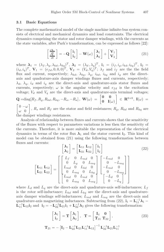
3.1 Basic Equations

The complete mathematical model of the single machine infinite-bus system con-sists of electrical and mechanical dynamics and load constraints. The electricaldynamics comprising the stator and rotor damper windings, with the currents asthe state variables, after Park’s transformation, can be expressed as follows [22]:

[dλ1dt

dλ2dt

]= −Q

[i1i2

]− W(ω)

[λ1λ2

]+

[V1V2

](21)

where λ1 = (λf , λg, λkd, λkq)T , λ2 = (λd , λq)T , i1 = (if , ig, ikd, ikq)T , i2 =(id, iq)T , V1 = (efd, 0, 0, 0)T , V2 = (Vd, Vq)T ; λf and if are the the fieldflux and current, respectively; λkd, λkq, λg, ikd, ikq and ig are the direct-axis and quadrature-axis damper windings fluxes and currents, respectively;λd, λq, id and iq are the direct-axis and quadrature-axis stator fluxes andcurrents, respectively; ω is the angular velocity and efd is the excitationvoltage; Vd and Vq are the direct-axis and quadrature-axis terminal voltages;

Q =diag[Rf , Rg, Rkd, Rkq , −Ra, −Ra] , W(ω) =[0 00 I(ω)

]∈ R6×6, I(ω) =

[0 −ωω 0

], Rs and Rf are the stator and field resistances; Rg, Rkd and Rkq are

the damper windings resistances.Analysis of relationship between fluxes and currents shows that the sensitivity

of the fluxes with respect to parameters variations is less then the sensitivity ofthe currents. Therefore, it is more suitable the representation of the electricaldynamics in terms of the rotor flux λ1 and the stator current i2. This kind ofmodel can be obtained from (21) using the following transformation betweenfluxes and currents: [

λ1λ2

]=

[L11 L12L21 L22

] [i1i2

](22)

[L11 L12L21 L22

]=

⎡

⎢⎢⎢⎢⎢⎢⎣

⎡

⎢⎢⎣

Lf 0 Lmd 00 Lg 0 Lmq

Lmd 0 Lkd 00 Lmq 0 Lkq

⎤

⎥⎥⎦

⎡

⎢⎢⎣

−Lmd 00 −Lmq

−Lmd 00 −Lmq

⎤

⎥⎥⎦

[Lmd 0 Lmd 0

0 Lmq 0 Lmq

] [−Ld 0

0 −Lq

]

⎤

⎥⎥⎥⎥⎥⎥⎦

where Ld and Lq are the direct-axis and quadrature-axis self-inductances; Lf

is the rotor self-inductance; Lkd and Lkq are the direct-axis and quadrature-axis damper windings self-inductances; Lmd and Lmq are the direct-axis andquadrature-axis magnetizing inductances. Subtracting from (22), i1 = L−1

11 λ1 −L−1

11 L12i2 and i2 = −L−122 L21i1 + L−1

22 λ2 gives the following transformation:[

λ1i2

]= T

[λ1λ2

], T =

[I4 0

T21 T22

], (23)

T21 = −[I2 − L−1

22 L21L−111 L12

]−1L−1

22 L21L−111

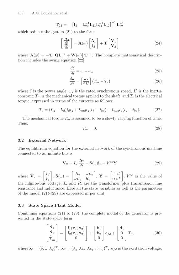
408 A.G. Loukianov et al.

T22 = −[I2 − L−1

22 L21L−111 L12

]−1L−1

22

which reduces the system (21) to the form[

dλ1dtdi2dt

]= A(ω)

[λ1i2

]+ T

[V1V2

](24)

where A(ω) = −T[QL−1 + W(ω)

]T−1. The complete mathematical descrip-

tion includes the swing equation [22]

dδ

dt= ω − ωs (25)

dω

dt=

[ ωs

2H

](Tm − Te) (26)

where δ is the power angle; ωs is the rated synchronous speed, H is the inertiaconstant; Tm is the mechanical torque applied to the shaft; and Te is the electricaltorque, expressed in terms of the currents as follows:

Te = (Lq − Ld)idiq + Lmdiq(if + ikd) − Lmqid(ig + ikq). (27)

The mechanical torque Tm is assumed to be a slowly varying function of time.Thus:

Tm = 0. (28)

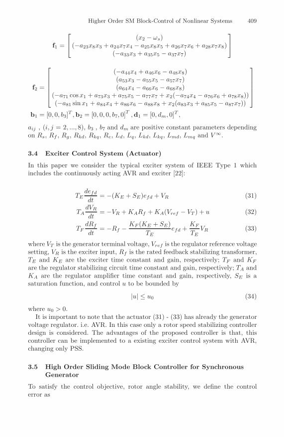
3.2 External Network

The equilibrium equation for the external network of the synchronous machineconnected to an infinite bus is

V2 = Ledi2dt

+ S(ω)i2 + V ∞Y (29)

where V2 =[

Vd

Vq

], S(ω) =

[Re −ωLe

ωLe Re

], Y =

[sin δcos δ

], V ∞ is the value of

the infinite-bus voltage; Le and Re are the transformer plus transmission lineresistance and inductance. Here all the state variables as well as the parametersof the model (21)-(29) are expressed in per unit.

3.3 State Space Plant Model

Combining equations (21) to (29), the complete model of the generator is pre-sented in the state-space form

⎡

⎢⎣

x1x2·Tm

⎤

⎥⎦ =

⎡

⎣f1(x1,x2)f2(x1,x2)

0

⎤

⎦ +

⎡

⎣b1b20

⎤

⎦ efd +

⎡

⎣d100

⎤

⎦Tm (30)

where x1 = (δ, ω, λf )T , x2 = (λg, λkd, λkq, id, iq)T , efd is the excitation voltage,

Higher Order SM Block-Control of Nonlinear Systems 409

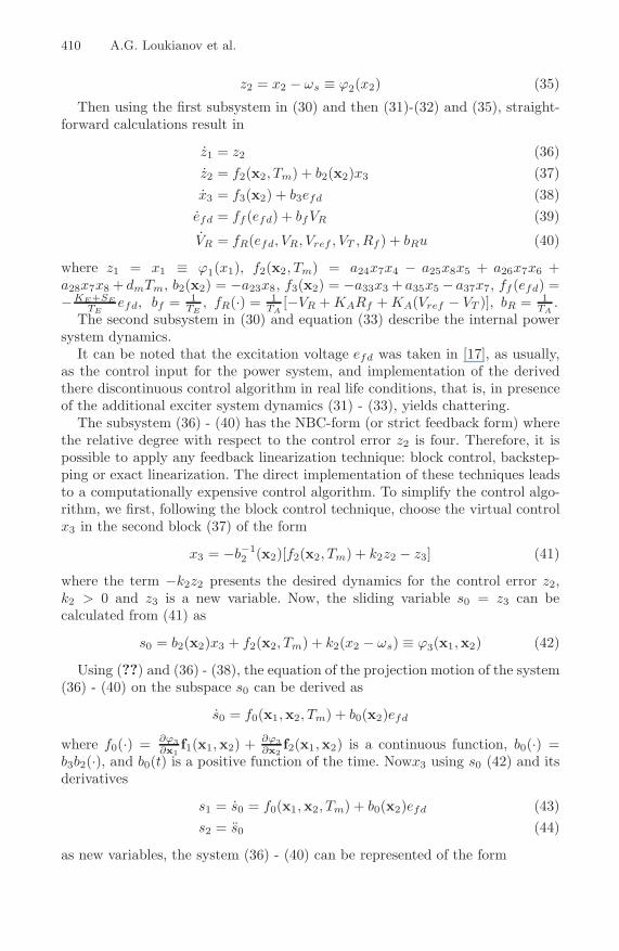
f1 =

⎡

⎣(x2 − ωs)

(−a23x8x3 + a24x7x4 − a25x8x5 + a26x7x6 + a28x7x8)(−a33x3 + a35x5 − a37x7)

⎤

⎦

f2 =

⎡

⎢⎢⎢⎢⎣

(−a44x4 + a46x6 − a48x8)(a53x3 − a55x5 − a57x7)(a64x4 − a66x6 − a68x8)

(−a71 cosx1 + a73x3 + a75x5 − a77x7 + x2(−a74x4 − a76x6 + a78x8))(−a81 sinx1 + a84x4 + a86x6 − a88x8 + x2(a83x3 + a85x5 − a87x7))

⎤

⎥⎥⎥⎥⎦

b1 = [0, 0, b3]T ,b2 = [0, 0, 0, b7, 0]T ,d1 = [0, dm, 0]T ,

aij , (i, j = 2, ..., 8), b3 , b7 and dm are positive constant parameters dependingon Rs, Rf , Rg, Rkd, Rkq, Re, Ld, Lq, Lkd, Lkq, Lmd, Lmq and V ∞.

3.4 Exciter Control System (Actuator)

In this paper we consider the typical exciter system of IEEE Type 1 whichincludes the continuously acting AVR and exciter [22]:

TEdefd

dt= −(KE + SE)efd + VR (31)

TAdVR

dt= −VR + KARf + KA(Vref − VT ) + u (32)

TFdRf

dt= −Rf − KF (KE + SE)

TEefd +

KF

TEVR (33)

where VT is the generator terminal voltage, Vref is the regulator reference voltagesetting, VR is the exciter input, Rf is the rated feedback stabilizing transformer,TE and KE are the exciter time constant and gain, respectively; TF and KF

are the regulator stabilizing circuit time constant and gain, respectively; TA andKA are the regulator amplifier time constant and gain, respectively, SE is asaturation function, and control u to be bounded by

|u| ≤ u0 (34)

where u0 > 0.It is important to note that the actuator (31) - (33) has already the generator

voltage regulator. i.e. AVR. In this case only a rotor speed stabilizing controllerdesign is considered. The advantages of the proposed controller is that, thiscontroller can be implemented to a existing exciter control system with AVR,changing only PSS.

3.5 High Order Sliding Mode Block Controller for SynchronousGenerator

To satisfy the control objective, rotor angle stability, we define the controlerror as

410 A.G. Loukianov et al.

z2 = x2 − ωs ≡ ϕ2(x2) (35)

Then using the first subsystem in (30) and then (31)-(32) and (35), straight-forward calculations result in

z1 = z2 (36)z2 = f2(x2, Tm) + b2(x2)x3 (37)x3 = f3(x2) + b3efd (38)

efd = ff (efd) + bfVR (39)

VR = fR(efd, VR, Vref , VT , Rf ) + bRu (40)

where z1 = x1 ≡ ϕ1(x1), f2(x2, Tm) = a24x7x4 − a25x8x5 + a26x7x6 +a28x7x8 + dmTm, b2(x2) = −a23x8, f3(x2) = −a33x3 + a35x5 − a37x7, ff(efd) =−KE+SE

TEefd, bf = 1

TE, fR(·) = 1

TA[−VR + KARf + KA(Vref − VT )], bR = 1

TA.

The second subsystem in (30) and equation (33) describe the internal powersystem dynamics.

It can be noted that the excitation voltage efd was taken in [17], as usually,as the control input for the power system, and implementation of the derivedthere discontinuous control algorithm in real life conditions, that is, in presenceof the additional exciter system dynamics (31) - (33), yields chattering.

The subsystem (36) - (40) has the NBC-form (or strict feedback form) wherethe relative degree with respect to the control error z2 is four. Therefore, it ispossible to apply any feedback linearization technique: block control, backstep-ping or exact linearization. The direct implementation of these techniques leadsto a computationally expensive control algorithm. To simplify the control algo-rithm, we first, following the block control technique, choose the virtual controlx3 in the second block (37) of the form

x3 = −b−12 (x2)[f2(x2, Tm) + k2z2 − z3] (41)

where the term −k2z2 presents the desired dynamics for the control error z2,k2 > 0 and z3 is a new variable. Now, the sliding variable s0 = z3 can becalculated from (41) as

s0 = b2(x2)x3 + f2(x2, Tm) + k2(x2 − ωs) ≡ ϕ3(x1,x2) (42)

Using (??) and (36) - (38), the equation of the projection motion of the system(36) - (40) on the subspace s0 can be derived as

s0 = f0(x1,x2, Tm) + b0(x2)efd

where f0(·) = ∂ϕ3∂x1

f1(x1,x2) + ∂ϕ3∂x2

f2(x1,x2) is a continuous function, b0(·) =b3b2(·), and b0(t) is a positive function of the time. Nowx3 using s0 (42) and itsderivatives

s1 = s0 = f0(x1,x2, Tm) + b0(x2)efd (43)s2 = s0 (44)

as new variables, the system (36) - (40) can be represented of the form

Higher Order SM Block-Control of Nonlinear Systems 411

z1 = z2 (45)z2 = −k2z2 + s0 (46)s0 = s1 (47)s1 = s2 (48)s2 = fs(x1,x2, Tm, efd, VR, Vref , VT , Rf) + bs(x2)u (49)

where fs(·) is a smooth function, and bs(·) = b0(·)bR, and bs(t) is a positivefunction of the time. Taking in the account that the subsystem (47) - (49) isof the third order and the constraint (34), we select the following third ordersliding mode algorithm (17)-(18):

u = −u0sign[s2 + 2(|s0|2 + |s1|3)16 sign(s1 + |s0|

23 )sign(s0)]. (50)

Under the following condition:

u0 > |ueq(x1,x2, Tm, efd, VR, Vref , VT , Rf )| , ueq(·) = b−1s (·)fs(·) (51)

the state vector of the closed-loop system (45) - (50) converges to the set

s0 = 0, s1 = 0, s2 = 0 (52)

in finite time, and sliding mode starts on (52) from this time [15]. The condition(51) defines the closed-loop system stability region and obviously holds for allthe possible values of Vref and Tm. The sliding motion on (52) is described bythe reduced order SM equation

z1 = z2, z2 = −k2z2, (53)x2 = f2(x1 ,x2) + b2ueq(x1,x2, Tm, efdss, VRss, Vref , VT , η) (54)η = −a1η − a2efdss + a3VRss, (55)

where η = Rf , a1 = 1TF

, a2 = KF (KE+SE)TF TE

, a3 = KF

TF TEand the steady state

values efdss and VRss are calculated as solutions for s1 = 0 (42) and s2 = 0 (43),respectively.

Note that the linear subsystem (53) described the linearized mechanical dy-namics, has the desired eigenvalue −k2, while the subsystem (54)-(55) repre-sents the rotor flux and exciter system internal dynamics. The second equationin (53) with k2 > 0 is asymptotically stable, hence lim

t→∞z2(t) = 0, and the angle

z1(t) = z1(0) +∫ ∞

0z2(γ)dγ tends to a steady state value δss as the control

error z2(t) tends to zero. The variables x2 and η are describing zero dynamicsof closed-loop system (45) - (50) on the invariant subspace

{z1 = δss, z2 = 0, s0 = 0, s1 = 0, s2 = 0, x2 ∈ R5, η ∈ R

}. (56)

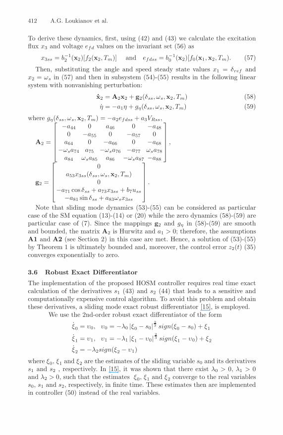
412 A.G. Loukianov et al.

To derive these dynamics, first, using (42) and (43) we calculate the excitationflux x3 and voltage efd values on the invariant set (56) as

x3ss = b−12 (x2)[f2(x2, Tm)] and efdss = b−1

0 (x2)[f0(x1,x2, Tm). (57)

Then, substituting the angle and speed steady state values x1 = δref andx2 = ωs in (57) and then in subsystem (54)-(55) results in the following linearsystem with nonvanishing perturbation:

x2 = A2x2 + g2(δss, ωs,x2, Tm) (58)η = −a1η + gη(δss, ωs,x2, Tm) (59)

where gη(δss, ωs,x2, Tm) = −a2efdss + a3VRss,

A2 =

⎡

⎢⎢⎢⎢⎣

−a44 0 a46 0 −a480 −a55 0 −a57 0

a64 0 −a66 0 −a68−ωsa74 a75 −ωsa76 −a77 ωsa78

a84 ωsa85 a86 −ωsa87 −a88

⎤

⎥⎥⎥⎥⎦

,

g2 =

⎡

⎢⎢⎢⎢⎣

0a53x3ss(δss, ωs,x2, Tm)

0−a71 cos δss + a73x3ss + b7uss

−a81 sin δss + a83ωsx3ss

⎤

⎥⎥⎥⎥⎦

.

Note that sliding mode dynamics (53)-(55) can be considered as particularcase of the SM equation (13)-(14) or (20) while the zero dynamics (58)-(59) areparticular case of (7). Since the mappings g2 and gη in (58)-(59) are smoothand bounded, the matrix A2 is Hurwitz and a1 > 0; therefore, the assumptionsA1 and A2 (see Section 2) in this case are met. Hence, a solution of (53)-(55)by Theorem 1 is ultimately bounded and, moreover, the control error z2(t) (35)converges exponentially to zero.

3.6 Robust Exact Differentiator

The implementation of the proposed HOSM controller requires real time exactcalculation of the derivatives s1 (43) and s2 (44) that leads to a sensitive andcomputationally expensive control algorithm. To avoid this problem and obtainthese derivatives, a sliding mode exact robust differentiator [15], is employed.

We use the 2nd-order robust exact differentiator of the form

ξ0 = υ0, υ0 = −λ0 |ξ0 − s0|23 sign(ξ0 − s0) + ξ1

ξ1 = υ1, υ1 = −λ1 |ξ1 − υ0|23 sign(ξ1 − υ0) + ξ2

ξ2 = −λ2sign(ξ2 − υ1)

where ξ0, ξ1 and ξ2 are the estimates of the sliding variable s0 and its derivativess1 and s2 , respectively. In [15], it was shown that there exist λ0 > 0, λ1 > 0and λ2 > 0, such that the estimates ξ0, ξ1 and ξ2 converge to the real variabless0, s1 and s2, respectively, in finite time. These estimates then are implementedin controller (50) instead of the real variables.

Higher Order SM Block-Control of Nonlinear Systems 413

3.7 Simulation Results

The performance of the proposed controller were tested on the complete 8th ordermodel of the generator connected to an infinite bus through a transmission line,Fig.1.

refV

TV

u

RV

PSS

AVR exciter

-

+

++

∑ ∑fde

sω ω−refV

TV

u

RV

PSS

AVR exciter

-

+

++

∑ ∑fde

sω ω−

Fig. 1. Diagram of excitation control system

The parameters of the synchronous machine and transmission system are (all inp.u., except where indicated): Rs =0.003, Rf =0.021, Rg =0.725, Rkd =10.714,Rkq =8.929, Ld =1.81, Lq =1.76, Lf =1.825, Lkd =1.831, Lkq =1.735, Re =0.05,H =3.525[s], ωs =377[rad s−1], Lmd =1.66, Lmq =1.61, Le =0.1. For these pa-rameters we obtain the parameters of mathematical model (30), : a23 =0.48514,a24 =-0.13789, a25 =0.46667, a26 =-0.8, a28 =0.02, am = 0.00003763, a33 =-0.71222, a35 =0.64556, a37 =-0.11067, a44 =2.776, a46 =-2.579, a48 =-0.322,a53 =30.321, a55 =-33.333, a57 =-5.000, a64 =9.849, a66 =-14.286, a68 =-7.143,a71 =-711.3, a73 =26.046±0.521, a74 =-0.26017, a75 =-28.759±0.118, a76 =-1.5008, a77 =-42.203, a78 =1.0377, b7 =345.08, a81 =-685.44, a83 =0.84848,a84=13.630, a85 =0.96364, a86 =-20.133, a87 =0.88207, a88 =-46.799. SettingTm = 0.9463 and V ∞ = 1, the steady state (or initial condition) is computed asx1(0) =1.3314, x2(0) =376.99, x3(0) =0.82038, x4(0) =-0.79228, x5(0) =0.62594,x6(0) =-0.79247, x7(0) =0.80354, and x8(0) =0.49319.

The controller gains were adjusted to u0 = 0.2, k0 = 10 and the constants forthe sliding differentiator were selected as λ0 = 125, λ1 = 115, and λ2 = 100.

Mechanical perturbations

..35.0 upTm = ..5.0 upTm =

Short circuit (0.15 sec).

sec.

Rad./sec.

ω

HOSM

AVR + PSS

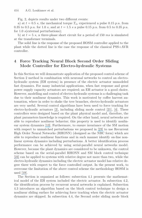
Fig. 2. Rotor velocity during mechanical perturbation and short circuit. Performancecomparison Sliding Mode v.s. AVR+PSS controller.

414 A.G. Loukianov et al.

Fig. 2, depicts results under two different events:a) at t = 0.5 s, the mechanical torque Tm experienced a pulse 0.15 p.u. from

0.35 to 0.5 p.u. for 1.0 s, and at t = 1.5 s a pulse 0.15 p.u. from 0.5 to 0.35 p.u.for 1.0 s(external perturbations);

b) at t = 5 s, a three-phase short circuit for a period of 150 ms is simulatedat the transformer terminals.

The solid line is the response of the proposed HOSM controller applied to theplant while the dotted line is the case the response of the classical PSS+AVRcontroller.

4 Force Tracking Neural Block Second Order SlidingMode Controller for Electro-hydraulic Systems

In this Section we will demonstrate application of the proposed control scheme ofSection 2 method in combination with neuronal networks to control an electro-hydraulic system (EH system) in presence of the electric actuator unmodeledfast dynamics. For many industrial applications, when fast response and greatpower supply capacity actuators are required; an EH actuator is a good choice.However, modelling and control of electro-hydraulic systems is a challenging taskdue to their nonlinear dynamics. This work is motivated by coffee harvest au-tomation, where in order to shake the tree branches, electro-hydraulic actuatorsare very useful. Several control algorithms have been used to force tracking forelectro-hydraulic actuators [2], including sliding mode control [21], [4]. Thesecontrollers were designed based on the plant physical model and, therefore, theplant parameters knowledge is required. On the other hand, neural networks areable to reproduce nonlinear behavior; this property is used to identify nonlin-ear system dynamics [13]. Furthermore, to ensure invariance of the SM motionwith respect to unmatched perturbations we proposed in [23] to use RecurrentHigh Order Neural Networks (RHONN) (designed as the NBC form) which areable to reproduce nonlinear functions and in such manner identify on-line non-linear system dynamics including perturbations. A better identification processperformance can be achieved by using serial-parallel neural networks model.However, because the plant dynamics are considered to be unknown, the controlscheme based on the serial-parallel RHONN and SM block control technique[23] can be applied to systems with relative degree not more than two, while theelectro-hydraulic dynamics including the electric actuator model has relative de-gree three with respect to the force controlled output. In the present work, toovercome the limitation of the above control scheme the methodology HOSM isused [19].

The Section is organized as follows: subsection 4.1 presents the mathemat-ical model of the EH system included the electric actuator. In subsection 4.2,the identification process by recurrent neural networks is explained. Subsection4.3 introduces an algorithm based on the block control technique to design anonlinear sliding surface for achieving force tracking when the electric actuatordynamics are skipped. In subsection 4.4, the Second order sliding mode block

Higher Order SM Block-Control of Nonlinear Systems 415

controller is designed taking in the account the electric actuator unmodeled dy-namics, and subsection 4.4 discusses results and simulations.

4.1 Mathematical Model

The complete mathematical model used to describe the behavior of the electro-hydraulic systems consists of the dynamics of a hydraulic actuator disturbed byan external load and dynamics of a servovalve. This model is separated in threeparts, the mechanical, hydraulic and servo-valve subsystems. In what follows,these parts are briefly described.

Mechanical subsystem

The piston disturbed by an external load, being modelled as a spring and adamper in parallel attached to the piston. Its dynamics can be derived using theNewton´s equation

ma =∑

fi = −ksxp − bdv + ΛaPL − Fr(v) (60)

where xp is the piston position, and vp = dxp

dt is the piston velocity, a is theacceleration of the piston,

∑fi represents the acting forces, PL is the load pres-

sure, Fr is the internal friction of the cylinder, m is the actuator mass, ks isthe load spring stiffness, bd is the load viscous damping, and Λa is the pistonarea. Using the state variables xp and vp and adding to (60) an unknown forceM(t) as a perturbation, the first two state space equations of the plant are thusgiven by

xp = vp (61)

vp =1m

(−ksxp − bdvp + ΛaPL − Fr(vp) − M(t)) (62)

The static friction model (Fr) [1] includes the Karnopp’s stick-slip friction [12]and Stribeck effect [3]. This function was programed in a Matlab/Simulink (atrademark of the Mathworks Inc.) table function to be used for the plant model.

Hydraulic subsystem

The dynamics of the cylinder are derived in [16] for a symmetric actuator. Defin-ing the load pressure to be the pressure across the actuator piston, the derivativeof the load pressure is given by the total load flow through the actuator dividedby the fluid capacitance:

Vt

4βe

PL = −Λaxp − CtmPL + QL (63)

where Vt is the total actuator volume, βe is the effective bulk modulus, Ctm isthe coefficient of total leakage due to pressure and QL is the turbulent hydraulic

416 A.G. Loukianov et al.

fluid flow through an orifice. The relationship between spool valve displacementxv, and the load flow QL, is given by

QL = Cdwxv

√Ps − sgn(xv)PL

ρ(64)

where xv is the valve spool position, Cd is the valve discharge coefficient, w isthe spool valve area gradient, Ps is the supply pressure and ρ is hydraulic fluiddensity. The spool area gradient for a cylindrical spool can be approximatedsimply as the circumference of the valve at each port. Combining (63) and (64)results in the load pressure state equation as

PL =4βe

Vt(−Λav − CtmPL) +

4βeCdwxv

Vt

√Ps − sgn(xv)PL

ρ

or equivalently

PL = −αvp − βPL +(γ√

Ps − sgn(xv)PL

)xv (65)

where α = 4Λaβe

Vt, β = 4Ctmβe

Vt, γ = 4Cdwβe

Vt√

ρ .

Servo-valve subsystem (actuator)

A frequency response analysis of the DDV-633 servo-valve in [16] establishedthat a second order system

xv = vv (66)vv = −anxv − bnvv + cnu (67)

where xv and vv are the valve spool position and velocity, respectively, and uis the servo-valve current input, an = 2.5676 × 105, bn = 6.2529 × 102 andcn = 2.4315 × 105 could describe adequate this behavior. Analysis of the modelshows the possibility to reduce the model order so that the dynamics of theservo-valve can be approximated by the first order system Xv(s)

U(s) = ka1/τ

s+(1/τ) or

xv = −1τxv +

ka

τu (68)

where τ = (1/573) s is the time constant, ka = 0.947 is the conversion gain.Fig. 3 portrays a diagram of the system which is utilized in this work.Combining equations (61), (62), (65) and (68), the electro-hydraulic model is

formulated in the spate-space form as

χ1 = χ2 (69)

χ2 =1m

(−ksχ1 − bdχ2 + Λaχ3 − Fr − M) (70)

χ3 = −αχ2 − βχ3 +(γ√

Ps − sgn(χ4)χ3

)χ4 (71)

χ4 = −1τχ4 +

ka

τu (72)

Higher Order SM Block-Control of Nonlinear Systems 417

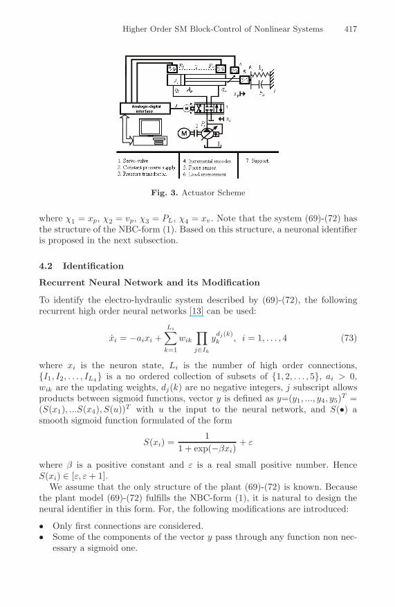
Fig. 3. Actuator Scheme

where χ1 = xp, χ2 = vp, χ3 = PL, χ4 = xv. Note that the system (69)-(72) hasthe structure of the NBC-form (1). Based on this structure, a neuronal identifieris proposed in the next subsection.

4.2 Identification

Recurrent Neural Network and its Modification

To identify the electro-hydraulic system described by (69)-(72), the followingrecurrent high order neural networks [13] can be used:

xi = −aixi +Li∑

k=1

wik

∏

j∈Ik

ydj(k)k , i = 1, . . . , 4 (73)

where xi is the neuron state, Li is the number of high order connections,{I1, I2, . . . , IL4} is a no ordered collection of subsets of {1, 2, . . . , 5}, ai > 0,wik are the updating weights, dj(k) are no negative integers, j subscript allowsproducts between sigmoid functions, vector y is defined as y=(y1, ..., y4, y5)T =(S(x1), ...S(x4), S(u))T with u the input to the neural network, and S(•) asmooth sigmoid function formulated of the form

S(xi) =1

1 + exp(−βxi)+ ε

where β is a positive constant and ε is a real small positive number. HenceS(xi) ∈ [ε, ε + 1].

We assume that the only structure of the plant (69)-(72) is known. Becausethe plant model (69)-(72) fulfills the NBC-form (1), it is natural to design theneural identifier in this form. For, the following modifications are introduced:

• Only first connections are considered.• Some of the components of the vector y pass through any function non nec-

essary a sigmoid one.

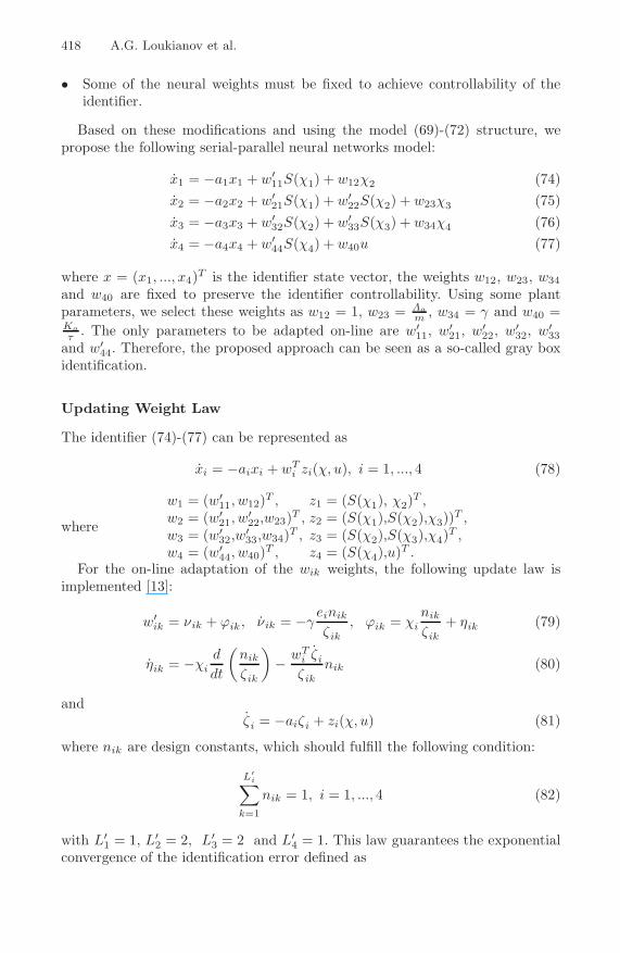
418 A.G. Loukianov et al.

• Some of the neural weights must be fixed to achieve controllability of theidentifier.

Based on these modifications and using the model (69)-(72) structure, wepropose the following serial-parallel neural networks model:

x1 = −a1x1 + w′11S(χ1) + w12χ2 (74)

x2 = −a2x2 + w′21S(χ1) + w′

22S(χ2) + w23χ3 (75)x3 = −a3x3 + w′

32S(χ2) + w′33S(χ3) + w34χ4 (76)

x4 = −a4x4 + w′44S(χ4) + w40u (77)

where x = (x1, ..., x4)T is the identifier state vector, the weights w12, w23, w34and w40 are fixed to preserve the identifier controllability. Using some plantparameters, we select these weights as w12 = 1, w23 = Λa

m , w34 = γ and w40 =Ka

τ . The only parameters to be adapted on-line are w′11, w′

21, w′22, w′

32, w′33

and w′44. Therefore, the proposed approach can be seen as a so-called gray box

identification.

Updating Weight Law

The identifier (74)-(77) can be represented as

xi = −aixi + wTi zi(χ, u), i = 1, ..., 4 (78)

where

w1 = (w′11, w12)T , z1 = (S(χ1), χ2)

T ,w2 = (w′

21, w′22,w23)T , z2 = (S(χ1),S(χ2),χ3))T ,

w3 = (w′32,w′

33,w34)T , z3 = (S(χ2),S(χ3),χ4)T ,w4 = (w′

44, w40)T , z4 = (S(χ4),u)T .For the on-line adaptation of the wik weights, the following update law is

implemented [13]:

w′ik = νik + ϕik, νik = −γ

einik

ζik

, ϕik = χi

nik

ζik

+ ηik (79)

ηik = −χi

d

dt

(nik

ζik

)− wT

i ζi

ζik

nik (80)

andζi = −aiζi + zi(χ, u) (81)

where nik are design constants, which should fulfill the following condition:

L′i∑

k=1

nik = 1, i = 1, ..., 4 (82)

with L′1 = 1, L′

2 = 2, L′3 = 2 and L′

4 = 1. This law guarantees the exponentialconvergence of the identification error defined as

Higher Order SM Block-Control of Nonlinear Systems 419

ei = xi − χi, i = 1, ..., 4

and the existence of bounds for the weights and their derivatives. For a detailedanalysis of this identification scheme, please see [13].

The proposed control scheme is based on the following assumption:B1) The systems (69)-(72) and (74)-(77) are input-to-state stable.

For a given desired trajectory, expressed on state variables as χref , a nonlinearsystem with state χ formulated as (69)-(72) and a neural network described by(74)-(77), it is possible to establish the following inequality:

∥∥χref − χ∥∥ ≤ ‖x − χ‖ +

∥∥χref − x∥∥

where ‖·‖ stands for the Euclidean norm. Hence, we introduce the followingconditions for the neural network tracking problem solution:

Identification Condition (ID)

limt→∞ ‖x(t) − χ(t)‖ = 0

Asymptotic Tracking Condition (AS)

limt→∞

∥∥χref (t) − x(t)

∥∥ = 0

In order to ensure the ID condition, an identifier based on neural network (74)-(77) with the on-line update law (79)-(82), will be used. Based on combining thesliding mode and block control techniques, a tracking algorithm which achievesthe AS condition, will be developed.

The implementation of the whole structure is as follows. First, the plant andidentifier evolute open loop being excited by a bounded input. After an initial-ization time, the loop is closed by a sliding mode tracking controller.

4.3 Ideal First Order Sliding Mode Block Controller

In this subsection, a first order sliding mode controller design for the ideal re-duced order plant is presented, and in subsection 4.4 the HOSM controller forthe real complete order plant, is designed.

As mentioned above, the control objective is to track a given force referencetrajectory. For this purpose only two RHONN states are considered, namely (76)and (77). This subsystem can be presented as the NBC-form consisting of twoblocks:

x3 = f3(•) + b3χ4 (83)x4 = f4(•) + b4u (84)

where f3(•) = −a3x3 + w′32S(χ2) + w′

33S(χ3), b3 = w34, f4(•) = −a4x4 +w′

44S(χ4) and b4 = w40 with the output y = x3.Once the identification is achieved, the RHONN (83)-(84) is considered as the

system model. Defining the tracking error as

420 A.G. Loukianov et al.

z3 = x3 − r(t) (85)

and taking the derivative of (85) along the trajectories of (83) results in

z3 = f3(•) + b3χ4 − r(t) (86)

orz3 = −a3x3 + w′

32S(χ2) + w′33S(χ3) + w34χ4 − r(t) (87)

where r(t) represents the desired trajectory for x3. Now we choose the desireddynamics for z3 of the form

z3 = −k3z3 + s, k3 > 0 (88)

Then the sliding variable s is defined from (88) and (87) as

s = −a3x3 + w′32S(χ2) + w′

33S(χ3) + w34χ4 − r(t) + k3z3 (89)

and the straightforward algebra reveals

s = f4(•) + b4u (90)

where f4(•) = −a3(f3(•) + b3χ4) + w′32S(χ2) + w′

32ddt [S(χ2)] + w′

33S(χ3) +w′

33ddt [S(χ3)] − w34[−a4χ4 + w′

44S(χ4)] − r(t) + k3(−k3z3 + z4), b4 = w34w40 >0 and the derivatives w′

32 and w′33 are defined in (79)-(82). Now we select a

discontinuous control asu = −Msign(s) (91)

where M > 0. Under the following condition:

M > b−14

∣∣f4(•)

∣∣ (92)

the variable s converges to zero in finite time. Then a sliding mode motionappears on the manifold s = 0. This motion is described by the first ordersystem

z3 = −k3z3 (93)

with the desired eigenvalue −k3. If k3 > 0 then the tracking error z3 tends expo-nentially to zero. Note the condition (92) defines the closed-loop system stabilityregion and obviously holds for all possible values of the load flow QL. Moreover,in [4], it was established that the zero dynamics presented by subsystem (69)and (70), when χ3 = r(t), are stable.

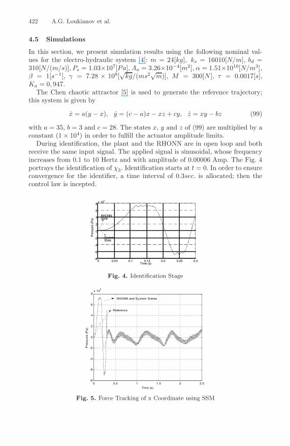
The implementation of the standard sliding mode (SSM) controller (91),however, leads to chattering in the closed-loop system, which is caused by thehigh-frequency switching of the sliding mode controller exciting the servo-valveunmodeled dynamics (67) (see Fig. 5 ).

Note that in [4] an observer was designed to avoid this chattering effect. How-ever, the observer implementation requires the plant parameters to be known.Therefore, in the next section we consider a chattering prevention scheme usingthe concept of second order sliding modes (SOSM) [7].

Higher Order SM Block-Control of Nonlinear Systems 421

4.4 Second Order Sliding Mode Block Controller

For the electro-hydraulic system under study, taking into account the completeservo-valve dynamics (66)-(67), the plant complete model has the relative degreetwo with respect to the designed output sliding function s (89). For that reason,the 2nd -order sliding mode controller is needed. We use a so called ”twisting”controller [7] in a combination with the second order robust differentiator [15].

Twisting algorithm

Using the new variables z3 (85), s0 = s = g4(•) + w34χ4, g4(•) = a3x3 +w32S(χ2) + w33S(χ3) − r(t) + k3z3 (89) and s1 = s0, the subsystem (83), (66)and (67) can be represented as

z3 = −k3z3 + s0 (94)s0 = s1 (95)s1 = fs(•) + bsu (96)

where χ5 = vv, fs(•) = d2

dt2 g4(•) − w34(anχ4 + bnχ5) and bs = w34cn.Considering that the subsystem (95) - (96) is of the second order, the following

twisting controller is implemented:

u(t) = −M0sign(s0) − M1sign(s1) (97)

In [7], it was shown that under the condition M0 > M1 >∣∣b−1

s fs(•)∣∣ , the state

of the closed-loop system converges to the set s0 = 0, s1 = 0 in finite time, andthen a sliding mode motion on this manifold will be governed by the desiredequation (93). For the implementation of the SOSM controller (97), it is onlynecessary to estimate s1.

Robust exact differentiation

To estimate the derivative s1 = s0 we use the following robust exact differentiatorvia sliding mode [15]:

z0 = z1 − λ0 |z0 − s|1/2 sign(z0 − s0) (98)z1 = −λ1sign(z0 − s0)

where λ0 and λ1 are positive constants, z0 is the estimate of s0 and z1 is theestimate of s1. If λ0 is taken sufficiently large with respect to λ1, then the 2nd

order sliding mode on

σ = z0 − s0 = 0

σ = λ0 |σ|1/2 sign(σ) + z1 + s1 = z1 + s1 = 0

will be established in finite time. The obtained estimate z1 is then used in thecontroller (97) instead of s1.

422 A.G. Loukianov et al.

4.5 Simulations

In this section, we present simulation results using the following nominal val-ues for the electro-hydraulic system [4]: m = 24[kg], ks = 16010[N/m], bd =310[N/(m/s)], Ps = 1.03×107[Pa], Λa = 3.26×10−4[m2], α = 1.51×1010[N/m3],β = 1[s−1], γ = 7.28 × 108[

√kg/(ms2√m)], M = 300[N ], τ = 0.0017[s],

Ka = 0, 947.The Chen chaotic attractor [5] is used to generate the reference trajectory;

this system is given by

x = a(y − x), y = (c − a)x − xz + cy, z = xy − bz (99)

with a = 35, b = 3 and c = 28. The states x, y and z of (99) are multiplied by aconstant (1 × 104) in order to fulfill the actuator amplitude limits.

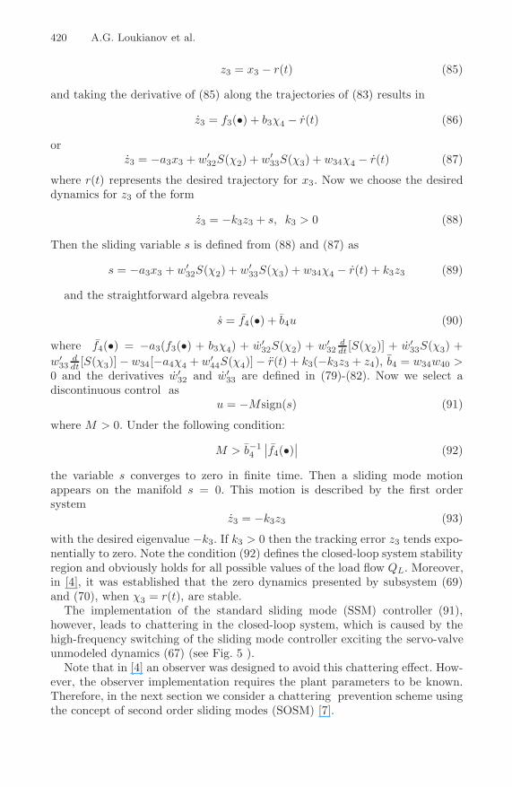
During identification, the plant and the RHONN are in open loop and bothreceive the same input signal. The applied signal is sinusoidal, whose frequencyincreases from 0.1 to 10 Hertz and with amplitude of 0.00006 Amp. The Fig. 4portrays the identification of χ3. Identification starts at t = 0. In order to ensureconvergence for the identifier, a time interval of 0.3sec. is allocated; then thecontrol law is incepted.

0 0.05 0.1 0.15 0.2 0.25 0.3-8

-6

-4

-2

0

2

4

6

8 x 105

Time (s)

Pre

ssur

e (P

a)

RHONNState

SystemState

0 0.05 0.1 0.15 0.2 0.25 0.3-8

-6

-4

-2

0

2

4

6

8 x 105

Time (s)

Pre

ssur

e (P

a)

RHONNState

SystemState

Fig. 4. Identification Stage

0 0.5 1 1.5 2 2.5-8

-6

-4

-2

0

2

4

6

8x 10

5

Time (s)

Pre

ssu

re (

Pa

)

RHONN and System States

Reference

Fig. 5. Force Tracking of x Coordinate using SSM

Higher Order SM Block-Control of Nonlinear Systems 423

0 0.5 1 1.5 2 2.5-8

-6

-4

-2

0

2

4

6

8x 10

5

Time (s)

Pre

ss

ure

(P

a)

RHONN and System States

Reference

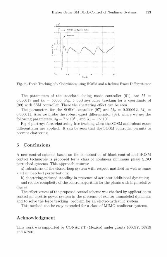
Fig. 6. Force Tracking of x Coordinate using HOSM and a Robust Exact Differentiator

The parameters of the standard sliding mode controller (91), are M =0.000017 and k3 = 50000. Fig. 5 portrays force tracking for x coordinate of(99) with SSM controller. There the chattering effect can be seen.

The parameters for the SOSM controller (97) are M0 = 0.000012, M1 =0.000011. Also we probe the robust exact differentiator (98), where we use thefollowing parameters: λ0 = 7 × 1011, and λ1 = 1 × 106.

Fig. 6 portrays force chattering-free tracking when the SOSM and robust exactdifferentiator are applied. It can be seen that the SOSM controller permits toprevent chattering.

5 Conclusions

A new control scheme, based on the combination of block control and HOSMcontrol techniques is proposed for a class of nonlinear minimum phase SISOperturbed systems. This approach ensures:

a) robustness of the closed-loop system with respect matched as well as somekind unmatched perturbations;

b) chattering-reduced stability in presence of actuator additional dynamics;and reduce complicity of the control algorithm for the plants with high relative

degree.The effectiveness of the proposed control scheme was checked by application to

control an electric power system in the presence of exciter unmodeled dynamicsand to solve the force tracking problem for an electro-hydraulic system.

This method can be easy extended for a class of MIMO nonlinear systems.

Acknowledgment

This work was supported by CONACYT (Mexico) under grants 46069Y, 56819and 57801.

424 A.G. Loukianov et al.

References

1. Alleyne, A., Liu, R.: Systematic control of a class of nonlinear systems with ap-plication to electrohydraulic cylinder pressure control. IEEE Transactions ControlSystems Technology 8, 623–634 (2000)

2. Akhkrif, O., Okou, F., Dessaint, L., Champagne, R.: Application of MultivariableFeedback Linearization Scheme for Rotor Angle Stability and Voltage Regulationof Power System. IEEE Trans. Power Syst. 14, 620–628 (1999)

3. Armstrong, B., Dupont, P., Canudas de Wit, C.: A Survey of analysis tools andcompensation methods for the control of machines with friction. Automatica 30,1083–1138 (1994)

4. Avila, M.A., Loukianov, A.G., Sanchez, E.N.: Electro-hydraulic actuator trajec-tory tracking. In: Proc. 2004 American Control Conference ACC 2004 (2004)

5. Chen, G., Ueta, T.: Yet another chaotic attractor. Int Journal of Bifurcation andChaos 9, 1465–1466 (1999)

6. Bazanella, A.S., Silva, A.S., Kokotovic, P.: Lyapunov Design of Excitation Controlfor Synchronous Machine. In: Proc. 1997 Conference on Decision and Control CDC1997 (1997)

7. Levant, A.: Sliding order and sliding accuracy in sliding mode control. InternationalJournal of Control 58, 1247–1263 (1993)

8. Fridman, L.: An averaging approach to chattering. IEEE Trans. Aut. Contr. 46,1260–1265 (2001)

9. Fridman, L., Loukianov, A., Canedo, J.M., Soto-Cota: A High order sliding modecontroller for synchronous generator with exciter system. IEEE Trans. On Indus-trial Electronics (to appear, 2008)

10. Galaz, M., Ortega, R., Bazanella, A., Stankovic, A.: An Energy-Shaping Approachto Excitation Control of Synchronous Generator. In: Proc 2001 American ControlConference ACC 2001 (2001)

11. Isidori, A.: Nonlinear control systems. Springer, London (1992)12. Karnopp, D.: Computer simulation of stick-slip friction in mechanical dynamic

systems. ASME Journal of Dynamic Systems, Measurement and Control 107, 100–103 (1985)

13. Kosmatopoulos, E.B., Christodoulou, M.A., Ioannou, P.A.: Dynamical neural net-works that ensure exponential identification error convergence. Int. Journal onNeural Networks 10, 299–314 (1997)

14. Krstic, M., Kanellakopoulos, I., Kokotovic, P.: Nonlinear and adaptive control de-sign. Wiley-Interscience, New York (1995)

15. Levant, A.: Higher-order sliding modes, differentiation and output-feedback con-trol. International Journal of Control 76, 924–941 (2003)

16. Liu, R.: Nonlinear control of electro-hydraulic servo-systems: Theory and experi-ment. MS thesis, Dept. Mech. Ind. Eng., Univ. Illinois (1998)

17. Loukianov, A.G., Canedo, J.M., Utkin, V.I., Cabrera-Vazquez, J.: Discontinuouscontroller for power system: sliding-mode block control approach. IEEE Trans. OnIndustrial Electronics 51, 340–353 (2004)

18. Loukianov, A.G.: Robust block decomposition sliding mode control design. Int.Journal on Mathematical Problems in Engineering: Theory, Methods and Appli-cations 8, 349–365 (2002)

19. Loukianov, A.G., Sanchez, E., Lizalde, C.: Force tracking neural block control foran electro-hydraulic actuator via second order sliding mode. International Journalof Robust abd Nonlinear Control 18, 319–332 (2007)

Higher Order SM Block-Control of Nonlinear Systems 425

20. Machowski, J., Robak, S., Bialek, J.W., Bumby, J.R., Abi-Samra, N.: Decentralizedstability-enhancing control of synchronous generator. IEEE Transactions on PowerSystems 15, 1336–1345 (2000)

21. Mohammed, J., Lamnabhi-Lagarrigue, F.: A new sliding mode controller for ahydraulic actuators. In: Proc. 2001 Conference on Decision and Control (2001)

22. Sauer, P.W., Pai, M.A.: Power system dynamics and stability. Prentice-Hall, NJ(1998)

23. Sanchez, E.N., Loukianov, A.G., Felix, R.A.: Recurrent neural block form control.Automatica 39, 1275–1282 (2003)

24. Son, K.M., Park, J.K.: On the robust LQR control of TCSC for damping powersystem oscillations. IEEE Trans. Power Syst. 15, 1306–1312 (2000)

25. Utkin, V.I., Guldner, J., Shi, J.: Sliding mode control in electromechanical systems.Taylor and Francis, London (1999)