High Throughput Sequencing Xiaole Shirley Liu STAT115, STAT215, BIO298, BIST520.

High Throughput Sequencing

Xiaole Shirley Liu

STAT115, STAT215, BIO298, BIST520

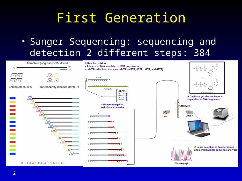
First Generation

• Sanger Sequencing: sequencing and detection 2 different steps: 384 * 1kb / 3 hours

2

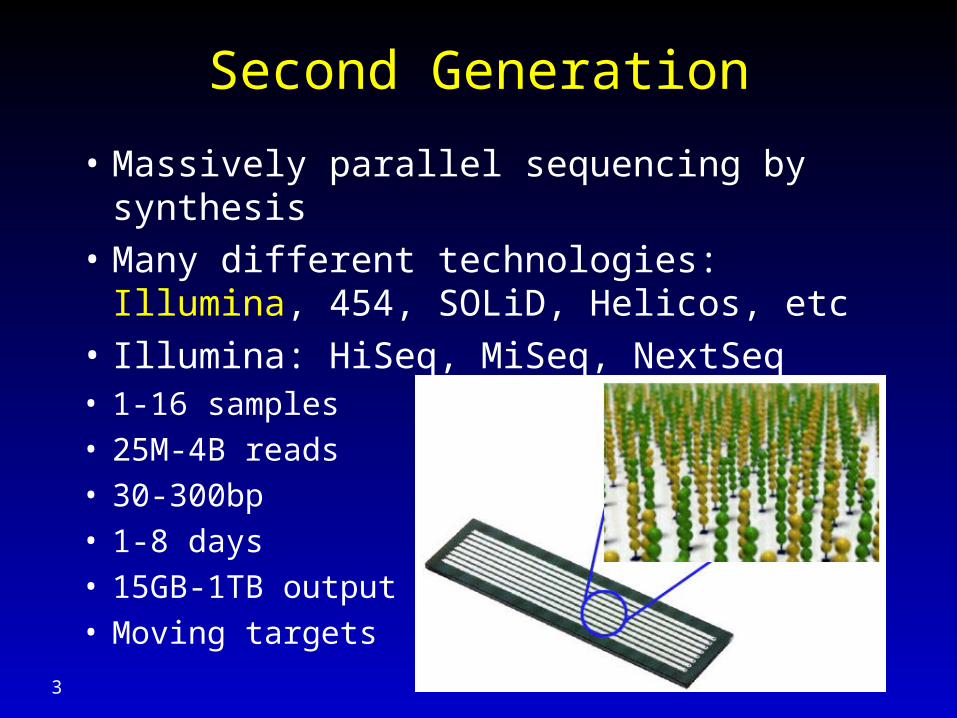
Second Generation

• Massively parallel sequencing by synthesis

• Many different technologies: Illumina, 454, SOLiD, Helicos, etc

• Illumina: HiSeq, MiSeq, NextSeq• 1-16 samples • 25M-4B reads• 30-300bp • 1-8 days• 15GB-1TB output• Moving targets

3

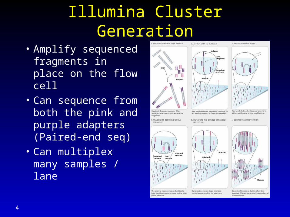
Illumina Cluster Generation

• Amplify sequenced fragments in place on the flow cell

• Can sequence from both the pink and purple adapters (Paired-end seq)

• Can multiplex many samples / lane

4

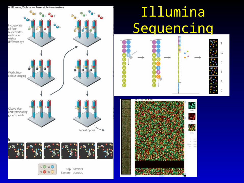
Illumina Sequencing

5

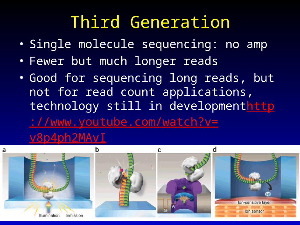
Third Generation• Single molecule sequencing: no amp• Fewer but much longer reads• Good for sequencing long reads, but not for read count

applications, technology still in developmenthttp://www.youtube.com/watch?v=v8p4ph2MAvI

• https://www.nanoporetech.com/news/movies#movie-28-minion

6

High Throughput Sequencing

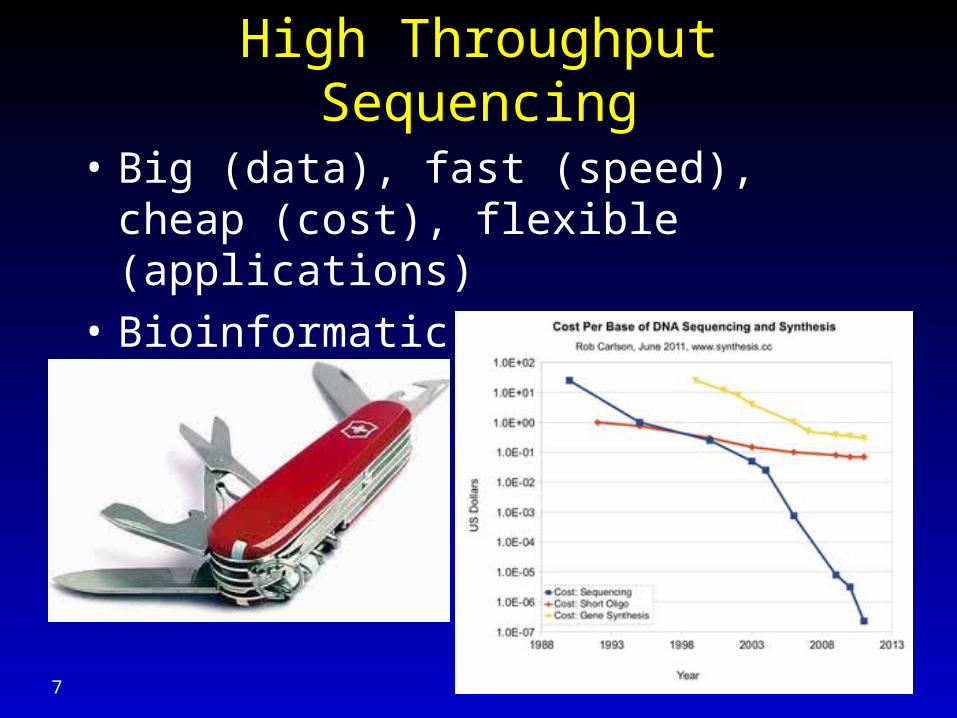
• Big (data), fast (speed), cheap (cost), flexible (applications)

• Bioinformatic analyses become bottleneck

7

High Throughput Sequencing Data Analysis

8

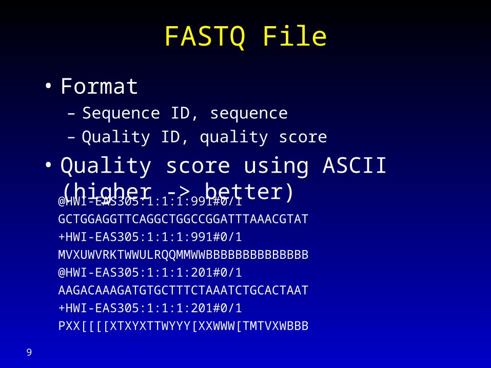
FASTQ File

• Format– Sequence ID, sequence

– Quality ID, quality score

• Quality score using ASCII (higher -> better)

9

@HWI-EAS305:1:1:1:991#0/1

GCTGGAGGTTCAGGCTGGCCGGATTTAAACGTAT

+HWI-EAS305:1:1:1:991#0/1

MVXUWVRKTWWULRQQMMWWBBBBBBBBBBBBBB

@HWI-EAS305:1:1:1:201#0/1

AAGACAAAGATGTGCTTTCTAAATCTGCACTAAT

+HWI-EAS305:1:1:1:201#0/1

PXX[[[[XTXYXTTWYYY[XXWWW[TMTVXWBBB

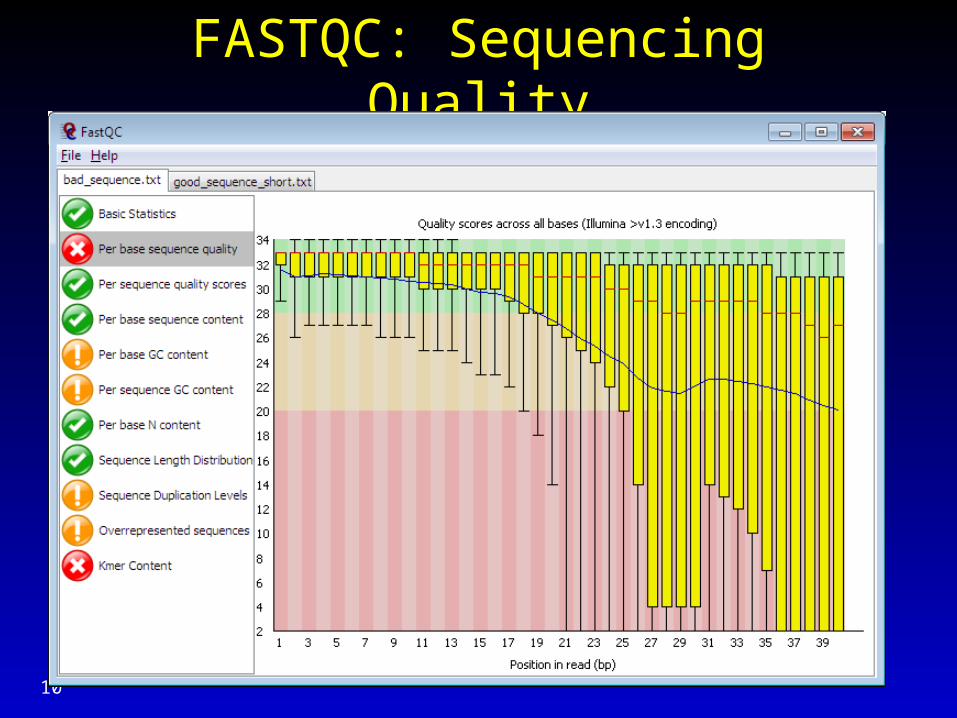
FASTQC: Sequencing Quality

10

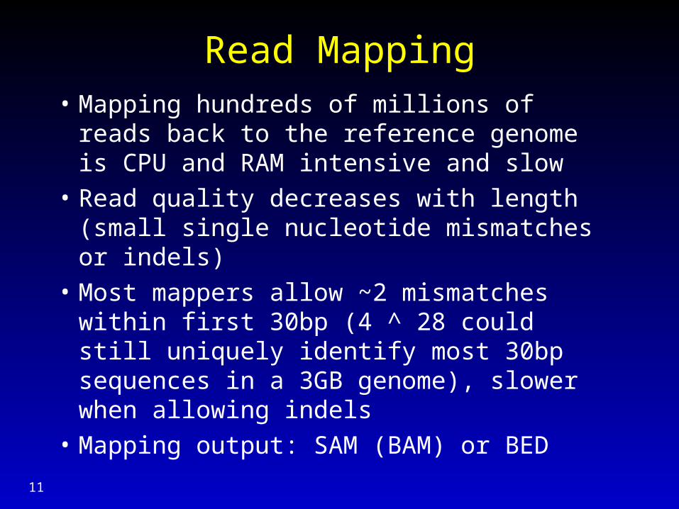
Read Mapping

• Mapping hundreds of millions of reads back to the reference genome is CPU and RAM intensive and slow

• Read quality decreases with length (small single nucleotide mismatches or indels)

• Most mappers allow ~2 mismatches within first 30bp (4 ^ 28 could still uniquely identify most 30bp sequences in a 3GB genome), slower when allowing indels

• Mapping output: SAM (BAM) or BED11

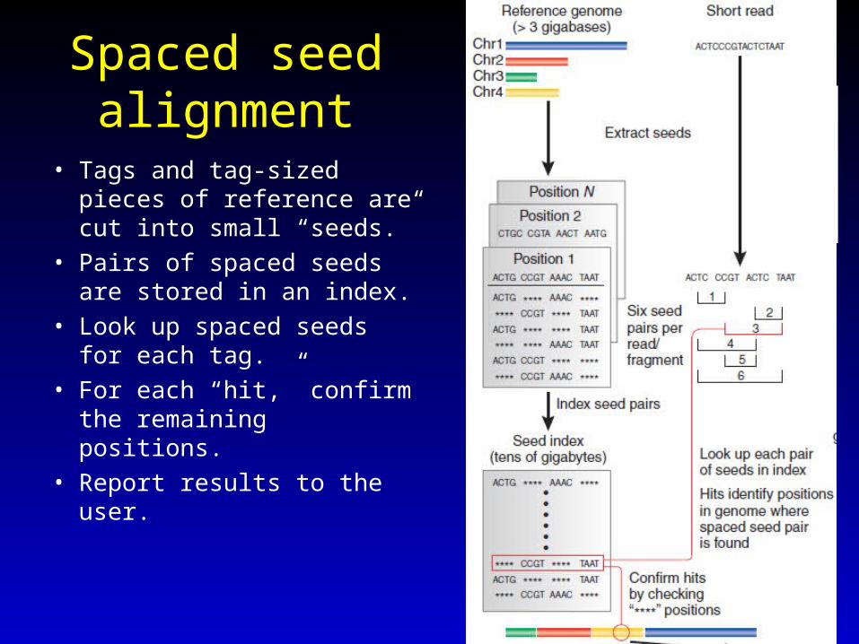
Spaced seed alignment

• Tags and tag-sized pieces of reference are cut into small “seeds.”

• Pairs of spaced seeds are stored in an index.

• Look up spaced seeds for each tag.

• For each “hit,” confirm the remaining positions.

• Report results to the user.

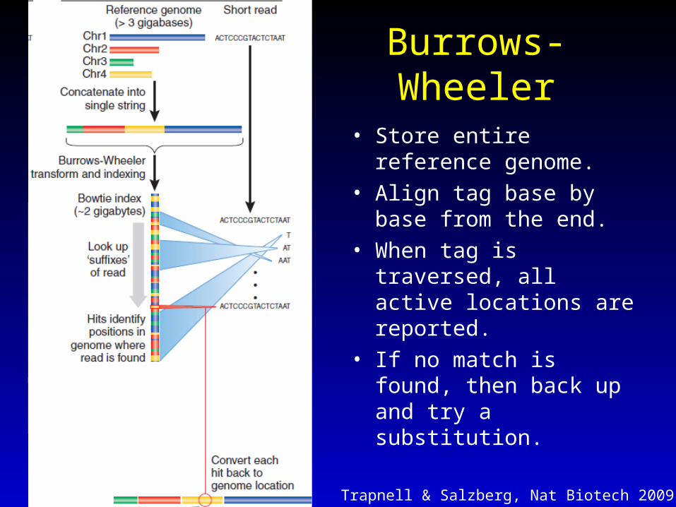
Burrows-Wheeler

• Store entire reference genome.

• Align tag base by base from the end.

• When tag is traversed, all active locations are reported.

• If no match is found, then back up and try a substitution.

Trapnell & Salzberg, Nat Biotech 2009

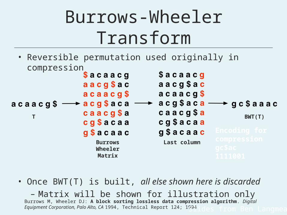
Burrows-Wheeler Transform

• Reversible permutation used originally in compression

• Once BWT(T) is built, all else shown here is discarded– Matrix will be shown for illustration only

BurrowsWheelerMatrix

Last column

BWT(T)T

Burrows M, Wheeler DJ: A block sorting lossless data compression algorithm. Digital Equipment Corporation, Palo Alto, CA 1994, Technical Report 124; 1994Slides from Ben Langmead

Encoding for compressiongc$ac1111001

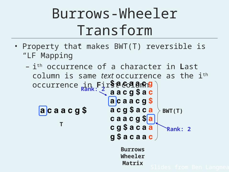
Burrows-Wheeler Transform

• Property that makes BWT(T) reversible is “LF Mapping”– ith occurrence of a character in Last column is

same text occurrence as the ith occurrence in First column

T

BWT(T)

Burrows WheelerMatrix

Rank: 2

Rank: 2

Slides from Ben Langmead

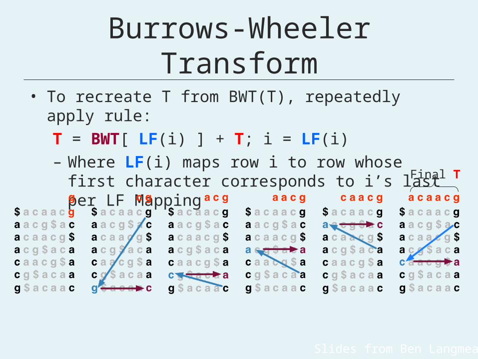
Burrows-Wheeler Transform

• To recreate T from BWT(T), repeatedly apply rule:T = BWT[ LF(i) ] + T; i = LF(i)– Where LF(i) maps row i to row whose first

character corresponds to i’s last per LF Mapping Final T

Slides from Ben Langmead

Exact Matching with FM Index

• To match Q in T using BWT(T), repeatedly apply rule:top = LF(top, qc); bot = LF(bot, qc)– Where qc is the next character in Q (right-to-

left) and LF(i, qc) maps row i to the row whose first character corresponds to i’s last character as if it were qc

Slides from Ben Langmead

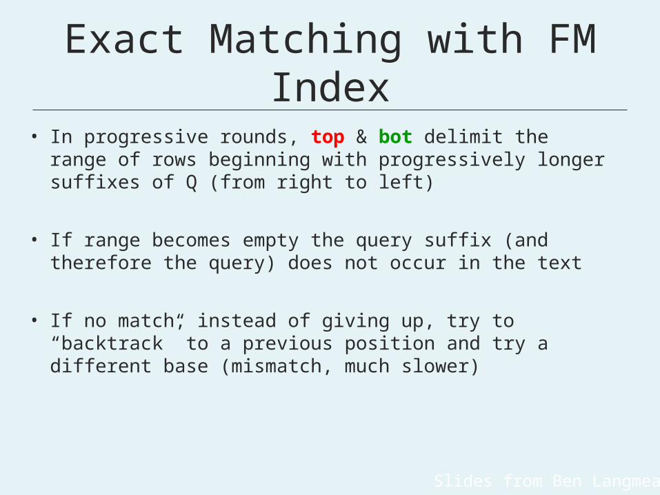
Exact Matching with FM Index

• In progressive rounds, top & bot delimit the range of rows beginning with progressively longer suffixes of Q (from right to left)

• If range becomes empty the query suffix (and therefore the query) does not occur in the text

• If no match, instead of giving up, try to “backtrack” to a previous position and try a different base (mismatch, much slower)

Slides from Ben Langmead

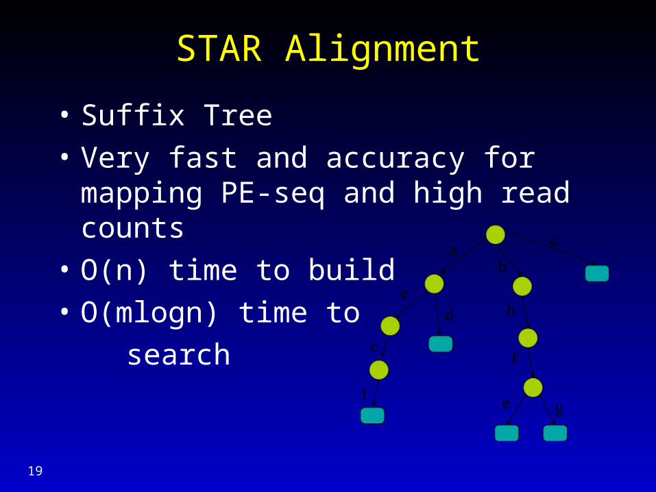
STAR Alignment

• Suffix Tree

• Very fast and accuracy for mapping PE-seq and high read counts

• O(n) time to build

• O(mlogn) time to

search

19

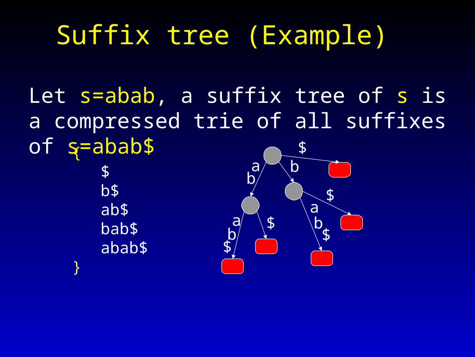
Suffix tree (Example)

Let s=abab, a suffix tree of s is a compressed trie of all suffixes of s=abab$

{ $ b$ ab$ bab$ abab$ }

ab

ab

$

ab$

b

$

$

$

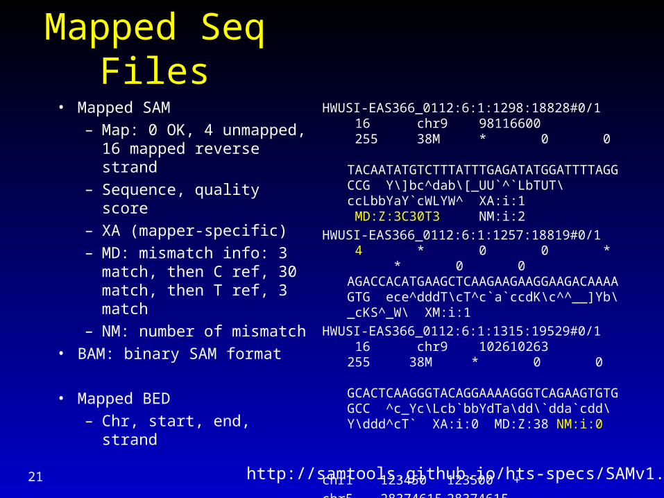
Mapped Seq Files

• Mapped SAM

– Map: 0 OK, 4 unmapped, 16 mapped reverse strand

– Sequence, quality score

– XA (mapper-specific)

– MD: mismatch info: 3 match, then C ref, 30 match, then T ref, 3 match

– NM: number of mismatch

• BAM: binary SAM format

• Mapped BED

– Chr, start, end, strand

21

HWUSI-EAS366_0112:6:1:1298:18828#0/1    16      chr9    98116600        255     38M     *       0       0       TACAATATGTCTTTATTTGAGATATGGATTTTAGGCCG  Y\]bc^dab\[_UU`^`LbTUT\ccLbbYaY`cWLYW^  XA:i:1  MD:Z:3C30T3     NM:i:2

HWUSI-EAS366_0112:6:1:1257:18819#0/1    4       *       0       0       *       *       0       0       AGACCACATGAAGCTCAAGAAGAAGGAAGACAAAAGTG  ece^dddT\cT^c`a`ccdK\c^^__]Yb\_cKS^_W\  XM:i:1

HWUSI-EAS366_0112:6:1:1315:19529#0/1    16      chr9    102610263       255     38M     *       0       0       GCACTCAAGGGTACAGGAAAAGGGTCAGAAGTGTGGCC  ^c_Yc\Lcb`bbYdTa\dd\`dda`cdd\Y\ddd^cT`  XA:i:0  MD:Z:38 NM:i:0

chr1 123450 123500 +chr5 2837461528374615-http://samtools.github.io/hts-specs/SAMv1.pdf

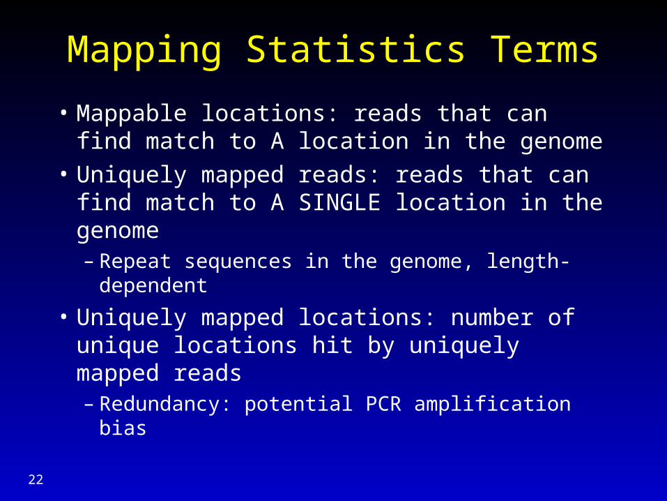
Mapping Statistics Terms

• Mappable locations: reads that can find match to A location in the genome

• Uniquely mapped reads: reads that can find match to A SINGLE location in the genome– Repeat sequences in the genome, length-

dependent

• Uniquely mapped locations: number of unique locations hit by uniquely mapped reads– Redundancy: potential PCR amplification bias

22

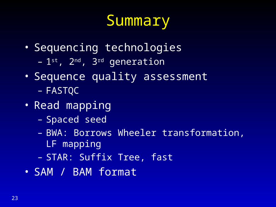
Summary

• Sequencing technologies– 1st, 2nd, 3rd generation

• Sequence quality assessment– FASTQC

• Read mapping– Spaced seed

– BWA: Borrows Wheeler transformation, LF mapping

– STAR: Suffix Tree, fast

• SAM / BAM format

23