Schlüsseltechnologien / Key Technologies Band / Volume 229 ISBN 978-3-95806-526-0 High-throughput All-Electron Density Functional Theory Simulations for a Data-driven Chemical Interpretation of X-ray Photoelectron Spectra Jens Bröder

Welcome message from author
This document is posted to help you gain knowledge. Please leave a comment to let me know what you think about it! Share it to your friends and learn new things together.
Transcript

Schlüsseltechnologien / Key TechnologiesBand / Volume 229ISBN 978-3-95806-526-0
High-throughput All-Electron Density Functional Theory Simulations for a Data-driven Chemical Interpretation of X-ray Photoelectron SpectraJens Bröder
High-throughput All-Electron
Density Functional Theory Simulations
for a Data-driven Chemical Interpretation of
X-ray Photoelectron Spectra
Von der Fakultät für Mathematik, Informatik und Naturwissenschaften der
RWTH Aachen University zur Erlangung des akademischen Grades eines
Doktors der Naturwissenschaften genehmigte Dissertation
vorgelegt von
M.Sc.
Jens Bröder
aus
Boppard
Berichter: Universitätsprofessor Dr. rer. nat. Stefan Blügel
Universitätsprofessor Dr. rer. nat. Riccardo Mazzarello
Universitätsprofessor Dr. rer. nat. Christian Linsmeier
Tag der mündlichen Prüfung: 12. August 2020
Diese Dissertation ist auf den Internetseiten der Universitätsbibliothek online
verfügbar.


Forschungszentrum Jülich GmbHPeter Grünberg Institut (PGI)Quanten-Theorie der Materialien (PGI-1/IAS-1)
High-throughput All-Electron Density Functional Theory Simulations for a Data-driven Chemical Interpretation of X-ray Photoelectron Spectra
Jens Bröder
Schriften des Forschungszentrums JülichReihe Schlüsseltechnologien / Key Technologies Band / Volume 229
ISSN 1866-1807 ISBN 978-3-95806-526-0

Bibliografische Information der Deutschen Nationalbibliothek. Die Deutsche Nationalbibliothek verzeichnet diese Publikation in der Deutschen Nationalbibliografie; detaillierte Bibliografische Daten sind im Internet über http://dnb.d-nb.de abrufbar.
Herausgeber Forschungszentrum Jülich GmbHund Vertrieb: Zentralbibliothek, Verlag 52425 Jülich Tel.: +49 2461 61-5368 Fax: +49 2461 61-6103 [email protected] www.fz-juelich.de/zb Umschlaggestaltung: Grafische Medien, Forschungszentrum Jülich GmbH
Druck: Grafische Medien, Forschungszentrum Jülich GmbH
Copyright: Forschungszentrum Jülich 2021
Schriften des Forschungszentrums JülichReihe Schlüsseltechnologien / Key Technologies, Band / Volume 229
D 82 (Diss. RWTH Aachen University, 2020)
ISSN 1866-1807ISBN 978-3-95806-526-0
Vollständig frei verfügbar über das Publikationsportal des Forschungszentrums Jülich (JuSER)unter www.fz-juelich.de/zb/openaccess.
This is an Open Access publication distributed under the terms of the Creative Commons Attribution License 4.0, which permits unrestricted use, distribution, and reproduction in any medium, provided the original work is properly cited.

For humanity and its AIs,
therefore most likely for you, the entity,
that is brave enough to be processing this.
— Journey before Destination —
- Brandon Sanderson
If you never fail, you are only trying things that are too easy
and playing far below your level.
- Eliezer, Yudkowsky
We do not only have to think about the future we want to live in,
we also have to lay it out and build it.
- MIT Essential knowledge: The Future


Abstract
Enabling computer-driven materials design to find and create materials with advanced prop-
erties from the enormous haystack of material phase space is a worthy goal for humanity. Most
high-technologies, for example in the energy or health sector, strongly depend on advanced
tailored materials. Since conventional research and screening of materials is rather slow and
expensive, being able to determine material properties on the computer poses a paradigm
shift. For the calculation of properties for pure materials on the nano scale ab initio methods
based on the theory of quantum mechanics are well established. Density Functional Theory
(DFT) is such a widely applied method from first principles with high predictive power.
To screen through larger sets of atomic configurations physical property calculation pro-
cesses need to be robust and automated. Automation is achieved through the deployment of
advanced frameworks which manage many workflows while tracking the provenance of data
and calculations. Through workflows, which are essential property calculator procedures, a
high-level automation environment is achievable and accumulated knowledge can be reused
by others. Workflows can be complex and include multiple programs solving problems over
several physical length scales.
In this work, the open source all-electron DFT program FLEUR implementing the highly
accurate Full-potential Linearized Augmented Plane Wave (FLAPW) method is connected
and deployed through the open source Automated Interactive Infrastructure and Database
for Computational Science (AiiDA) framework to achieve automation. AiiDA is a Python
framework which is capable of provenance tracking millions of high-throughput simulations
and their data. Basic and advanced workflows are implemented in an open source Python
package AiiDA-FLEUR, especially to calculate properties for the chemical analysis of X-ray
photoemission spectra. These workflows are applied on a wide range of materials, in particular
on most known metallic binary compounds.
The chemical-phase composition and other material properties of a surface region can be
understood through the careful chemical analysis of high-resolution X-ray photoemission
spectra. The spectra evaluation process is improved through the development of a fitting
method driven by data from ab initio simulations. For complex multi-phase spectra this pro-
posed evaluation process is expected to have advantages over the widely applied conventional
methods. The spectra evaluation process is successfully deployed on well-behaved spectra of
materials relevant for the inner wall (blanket and divertor) plasma-facing components of a
nuclear fusion reactor. In particular, the binary beryllium systems Be-Ti, Be-W and Be-Ta are
investigated. Furthermore, different approaches to calculate spectral properties like chemical
shifts and binding energies are studied and benchmarked against the experimental literature
and data from the NIST X-ray photoelectron spectroscopy database.
Kurzfassung
Viele Hochtechnologien, wie die Kernfusion sind stark auf maßgeschneiderte hochspezial-
isierte Materialien angewiesen. Die Ermöglichung von computergestüzter Materialentwick-
lung ist somit ein lohnenswertes Ziel der Menschheit, um aus dem riesigen Heuhaufen des
Materialphasenraumes High-tech Materialien mit gewollten Eigenschaften zu designen. Für
reine Materialien auf kleinen Lägenskalen sind etablierte ab initio Methoden, welche auf der
Theorie der Quantenmechanik basieren, wie die Dichtefunktionaltheorie (DFT) der Stand
der Technik, um Materialeigenschaften mit Hilfe des Computers zu bestimmen, bevor diese
Materialien im Labor langsam und kostenintensiv überprüft werden.
Für computergestützte Materialentwicklung müssen Prozesse zur Berechnung von physikalis-
chen Eigenschaften robust und automatisiert werden, um Berechnungen an größeren Mengen
von Kristallstrukturkonfigurationen durchführen zu können. Die Automatisierung wird durch
den Einsatz hochentwickelter Frameworks erreicht, welche die Herkunft von Daten und
Berechnungen verfolgen und verwalten. Durch sogennante Workflows, welche Protokolle zur
physikalischen Eigenschaftsberechnung darstellen, wird ein hohes Maß an Automatisierung
erreicht und Expertenwissen kann in diesen konserviert und von anderen wiederverwendet
werden.
In dieser Arbeit wurde das Open-Source DFT-Programm FLEUR für die anstehenden
Aufgaben ausgewählt, welches alle Elektronen mithilfe der leistungsfähigen, hochpräzisen
Linearized Augmentierte Plane Wave (FLAPW) behandelt. Der FLEUR-Program wird an das
Open-Source Automated Interactive Infrastructure und Datenbank für Computational Sci-
ence (AiiDA) Framework angebunden, um eine hohe Automatisierung mit FLEUR erreichen
zu können. AiiDA ist ein Python-Framework, das millionen an Hochdurchsatzsimulatio-
nen und ihre Daten in einer Datenbank nachverfolgen und verwalten kann. Fundamentale
und fortgeschrittene Workflows wurden in einem Open-Source Python-Paket (AiiDA-FLEUR)
implementiert, um insbesondere Eigenschaften für die chemische Analyse von Röntgen-
photoelektronenspektren zu berechnen. Diese Workflows wurden auf eine Vielzahl von
Materialien angewendet, insbesondere auf bekannte, metallische, binäre Verbindungen.
Die genaue Phasenzusammensetzung und andere Eigenschaften eines oberflächennahen
Materials können durch die sorgfältige chemische Analyse von hochauflösenden Röntgen-
photoelektronenspektren verstanden werden. In dieser Arbeit wird der Spektrenauswer-
tungsprozess basierend auf ab initio Simulations Ergebnissen durch die Entwicklung einer
Anpassungsmethode für vorerst einfache, Mehrphasenspektren verbessert. Dieses XPS-
Auswertungsverfahren mit ab initio-Daten wurde erfolgreich auf Spektren von Materialien
angewendet, die für die Wandkomponenten eines Kernfusionsreaktors relevant sind, ins-
besondere für die Berylliumverbindungen (Be-Ti, Be-W, Be-Ta). Weitere Ansätze zur Berech-

nung der Spektren-Eigenschaften wie chemische Verschiebungen und Bindungsenergien
wurden untersucht und mit der experimentellen Literatur, insbesondere der NIST Datenbank
für Röntgenphotoelektronenspektroskopie verglichen.
v


Table of Contents
1. Introduction 1
2. Basics: Theory and Scientific Context 5
2.1. Interlude: Large Numbers in Perspective . . . . . . . . . . . . . . . . . . . . . . . 7
2.2. Massaging the Many-Body Problem . . . . . . . . . . . . . . . . . . . . . . . . . . 9
2.3. Density Functional Theory (DFT) . . . . . . . . . . . . . . . . . . . . . . . . . . . 10
2.3.1. Enthalpy of formation from DFT . . . . . . . . . . . . . . . . . . . . . . . . 16
2.4. The FLAPW method and the FLEUR program . . . . . . . . . . . . . . . . . . . . 17
2.5. Chemical Configuration Space, the second exponential wall . . . . . . . . . . . . 19
2.5.1. Crystal Structure Sources . . . . . . . . . . . . . . . . . . . . . . . . . . . . 20
2.5.2. Crystal Structure Discovery . . . . . . . . . . . . . . . . . . . . . . . . . . . 23
2.6. High-throughput Computation in Material Science . . . . . . . . . . . . . . . . . 25
2.7. The AiiDA framework . . . . . . . . . . . . . . . . . . . . . . . . . . . . . . . . . . . 27
2.7.1. Plug-ins in AiiDA . . . . . . . . . . . . . . . . . . . . . . . . . . . . . . . . . 31
2.7.2. Scientific Workflows (Workchains) in AiiDA . . . . . . . . . . . . . . . . . 31
2.7.3. The AiiDA Community and the Python Universe . . . . . . . . . . . . . . 33
2.8. Machine Learning in Material Science . . . . . . . . . . . . . . . . . . . . . . . . . 34
2.9. X-ray Photoelectron Spectroscopy (XPS) . . . . . . . . . . . . . . . . . . . . . . . 35
2.9.1. Current Chemical Interpretation of XPS . . . . . . . . . . . . . . . . . . . . 41
2.9.2. Quantities for XPS from ab initio Simulations . . . . . . . . . . . . . . . . 45
3. Method Development 49
3.1. The AiiDA-FLEUR Package . . . . . . . . . . . . . . . . . . . . . . . . . . . . . . . 49
3.1.1. Plug-in Layouts . . . . . . . . . . . . . . . . . . . . . . . . . . . . . . . . . . 50
3.1.2. Implemented Workflows for FLEUR . . . . . . . . . . . . . . . . . . . . . . 55
3.1.3. Core-level Spectra Turn-key Solution . . . . . . . . . . . . . . . . . . . . . 68
3.1.4. XPS Spectra Visualization App . . . . . . . . . . . . . . . . . . . . . . . . . 77
3.2. Fitting XPS Spectra from a Complete ab initio Dataset . . . . . . . . . . . . . . . 79
3.3. Method Development Sum-up . . . . . . . . . . . . . . . . . . . . . . . . . . . . . 84
vii

Table of Contents
4. Ab initio Simulation Results 854.1. Lessons from over 800 000 FLEUR Input Files . . . . . . . . . . . . . . . . . . . . 86
4.2. Material Screening: Creating a Core-Level Shift Database . . . . . . . . . . . . . 93
4.2.1. Data Quality and Robustness . . . . . . . . . . . . . . . . . . . . . . . . . . 109
4.2.2. Conclusion and Outlook Screening . . . . . . . . . . . . . . . . . . . . . . 109
4.3. Example: Fusion Relevant Materials . . . . . . . . . . . . . . . . . . . . . . . . . . 110
4.3.1. The Be-W System . . . . . . . . . . . . . . . . . . . . . . . . . . . . . . . . . 112
4.3.2. The Be-Ti System . . . . . . . . . . . . . . . . . . . . . . . . . . . . . . . . . 121
4.3.3. The Be-Ta System . . . . . . . . . . . . . . . . . . . . . . . . . . . . . . . . . 132
4.3.4. Core-level Shifts of selected other Systems . . . . . . . . . . . . . . . . . . 143
4.4. Ab initio Simulation Results Sum-up . . . . . . . . . . . . . . . . . . . . . . . . . . 150
5. Conclusion and Outlook 153
Appendices 157
A.Software Stack 159
B.Code and Data Visualization 161B.1. AiiDA Database Overview . . . . . . . . . . . . . . . . . . . . . . . . . . . . . . . . 161
B.2. Disk footprint Overview . . . . . . . . . . . . . . . . . . . . . . . . . . . . . . . . . 163
B.3. Repository Code Overview . . . . . . . . . . . . . . . . . . . . . . . . . . . . . . . . 164
viii

1. Introduction
Meeting the growing demands of over 9 billion human beings and the transition into a
longterm sustainable way of life on earth, while increasing or at least maintaining the status
and quality of human civilization and protecting our common goods [1, 2] is the grand chal-
lenge of our times. This is formulated by the United Nations general assembly in 17 sustainable
development goals to meet by 2030 [3, 4]. Materials production, usage and management play
a crucial role in our socioeconomic systems and heavily impact our environment [5].
Many technologies strongly depend on special materials with desired, optimized proper-
ties, designed form and economic feasibility [6, 7]. In the energy sector for example, solar
cells fully depend on materials with the right optical properties that yield a high quantum
efficiency while being inexpensive and durable enough to work for decades or longer [8–12].
Wind turbine blades and turbines in general also consist of optimized high-tech materials to
withstand forces and heat [13, 14]. Transitioning to a complete renewable energy mix crucially
depends on finding reasonable inexpensive materials for energy storage [15, 16] in large
quantities, especially for electric energy [17]. The challenge of making nuclear fusion a reality
depends from a technological point of view to a large extent on designing high-tech materials
that possess and sustain their desired properties long enough under the extreme operating
conditions of such a device [18, 19]. The durability, efficiency and economic feasibility of fuel
cells depends strongly on the cells materials [20]. Other challenges worth mentioning are new
permanent [21] or special magnets [22, 23], thermoelectrics [24], materials for (green) infor-
mation technologies, (quantum)computing [25], (high-temperature) superconductors [26],
lasers, (space)flight, materials for medical equipment [27], drugs [28], biofriendly materials
[29], catalysts [30], 3D printable materials, replacements for toxic, expensive, rare or oil based
materials.
The size of material phase space is enormous [31, 32] making it inconvenient and very costly
to optimize and screen materials through a pure experimental approach within laboratories,
like Edison [33] did for the filament of the electric light bulb, or Haber and Bosch pursued to
find a suitable catalyst for ammonia synthesis transforming agriculture worldwide [34]. Since
1993, worldwide computational capabilities increased [35] exponentially by a factor of over 1
million. Given these challenges and opportunities for materials, one worthy longtime goal
1
1. Introduction
pursued by mankind is to enable full scale computational/virtual data-driven materials design
[36–40]. An exemplary computer-driven process for the advancement or replacement of a
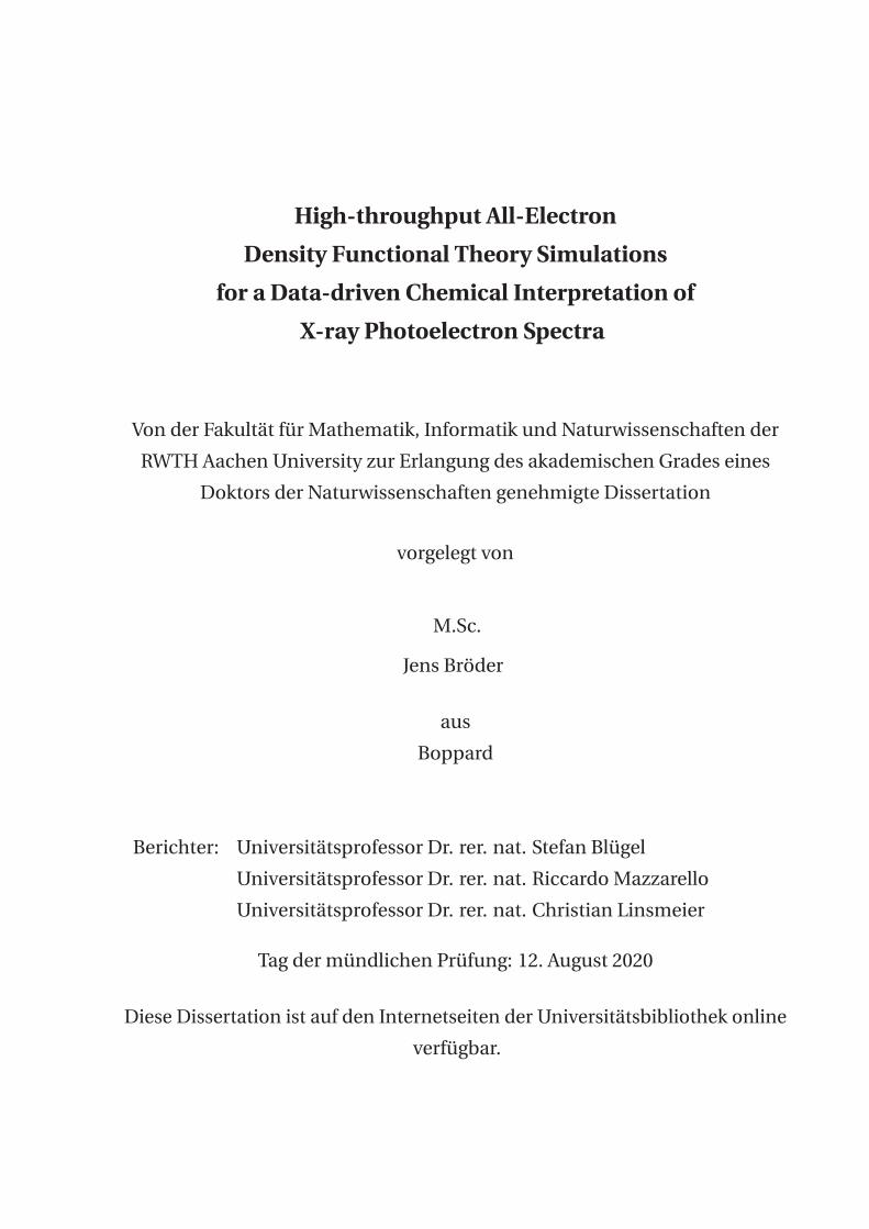
Fig. 1.1.: Materials-design process example for improvement of a high-tech material for a
device. Graphic under creative common license 3.0 taken as original from [37].
functional material is sketched in Fig. 1.1. After the characterization of the device and deciding
which properties need to be optimized and how, the discovery of new promising candidates
is done to a large extent on the computer deploying software from the materials informatics
toolbox [41–43] and utilizing various types of data available on materials. The suggested
promising candidate materials are then synthesized, tested in the laboratory, manufactured
and finally deployed, if the properties are satisfactory.
While the fundamental quantum mechanical equations for materials [44–46] are long
known in condensed matter physics and quantum chemistry, calculating material properties
accurately, i.e. solving these equations for a real world material like steel, is computationally
expensive or even impossible [47]. Since the micro structure (atomic configuration) of a
material determines its physical and chemical properties to a large extent, also the size of
material configuration space poses a challenge. It is growing exponentially with the number
of atoms or protons in a structure. This makes materials design a multi-scale problem. On the
one hand materials-informatics software [37, 42, 43, 48–50] has to be robust and automatized
to enable screening through many different materials, on the other hand practical models and
approximations for all length scales and diverse phenomena have to be created, implemented
and interconnected. Furthermore, massive amounts of data of all facets on materials have to
be shared and made available for others to harvest and progress [51]. Data repositories like
[39, 52–59] enable the deployment of machine learning techniques to discover correlations
and develop better models and understanding of the underlying physics [60].
2

To calculate material properties on the nano scale for molecules and solids established
practical ab initio methods, based on the theory of quantum mechanics [47], like Density
Functional Theory (DFT) [61] are the methods of choice. Archiving some degree of automation
in materials design processes is possible through the deployment of software frameworks [62–
72] which manage workflows and track the provenance of data and calculations. This ensures
the reliability and reproducibility of calculations. With property calculator protocols, so called
workflows, a high-level work environment is achievable. Through workflows knowledge can
accumulated and be rather easily reused by others. Workflows can involve multiple different
software packages connecting multiple physical scales in one solution. Besides depending
on the robustness and fidelity of the deployed software packages, a high overall fidelity of
a workflow is achievable through optimization and error treatment strategies within the
workflow itself.
In material research and quality assessment sample characterization and chemical phase
identification play an essential role. The same is true when studying surface and material
changes under external influences. For the identification of the crystal structure and large
solid periodic phases X-ray diffraction (XRD) [73, 74] is the state of the art technique. Insight
into the elemental composition can be provided by different scattering or scanning probes,
also through X-ray photoemission spectroscopy (XPS). For the determination of the chemical
phase composition of a sample, XPS or formally known as electron spectroscopy for chemical
analysis (ESCA) is the method of choice. XPS is a well known and widely applied technique in
research and industry [75–77]. The detailed evaluation of multi-phase high-resolution XPS
spectra is often challenging in practice [78].
This work advances a solution for the basic chemical material characterization with X-ray
photoemission spectroscopy. The underlying models and methods applied are known, but
have to be automated, advanced and connected to different tools to provide a low cost solution
for a broader set of materials in order to be useful to a broader audience. For the calculation
of spectral properties the open source all-electron DFT program, FLEUR [79] implementing
the powerful, highly accurate Linearized Augmented Plane Wave method (FLAPW) [80, 81]
was chosen. For automation the FLEUR program was connected to the AiiDA framework [63]
and workflows were implemented to calculate a range of material properties. As proof of
principle these workflows are deployed within a material screening project on most known
binary metals. These ab initio results are partly compared to findings of other DFT software
packages. In addition, selected ab initio results of beryllides (Be-W, Be-Ti, Be-Ta) relevant for
the plasma-facing components of a nuclear-fusion reactor [82] like for the International Ther-
monuclear Experimental Reactor (ITER) are discussed in more detail. These ab initio results
are compared to experimental X-ray photoelectron spectra data [83] which was measured by
3

1. Introduction
Nicola Helfer and others. The spectra of these beryllide systems are chemically interpreted
through ab initio core-level shift data obtained within this work.
The thesis is structured as follows. In Chapter 2 the basic background knowledge and
scientific context for this work is covered. The first sections of Chapter 2 describe the nature
of the many-body problem. They promote how material properties can be calculated from
density functional theory. The FLAPW method and its implementation in the FLEUR program
are covered in more detail, since FLEUR was deployed throughout this work. The challenges
of chemical, material configuration space and how these are tackled, among other knowledge,
with high-throughput simulations and machine learning is pointed out. A collection of the
current ab initio simulation databases and repositories is also presented in this chapter.
Developed methods within this thesis are discussed in Chapter 3. One section in this chapter
discusses the developed open source AiiDA-FLEUR package, which enables high-throughput
calculations with the FLEUR program using the AiiDA framework. Furthermore, plug-in
layouts and implemented workflows around FLEUR are described. The description includes
the self-consistency field workflow, a density of states, a band structure workflow, a workflow
to calculate an equation of states and workflows for the calculation of core-level shifts and
core-level binding energies. A deployable small search and visualize application (Jupyter
App) and visualization functions for spectral data are discussed in this chapter. Another
section introduces how well-behaved mixed X-ray photoelectron spectra can be fitted from
constructed spectra of ab initio data. From this physically motivated constrained fit the
chemical interpretation of the spectra is possible.
In Chapter 4 selected ab initio simulation results, produced with the deployment of the
developed methods, are reported. The first sections discuss what needs to be known, in
order to enable material screening projects with high all-electron simulation success rates.
This involves the control of good FLAPW parameters and knowing the convergence behavior
of quantities of interest. The results from a small screening project of most known metal
binary materials is discussed. The FLEUR simulation results are compared to experimental
databases and results from other electronic structure programs. Furthermore, ab initio results
of beryllides (Be-W, Be-Ti, Be-Ta) relevant for the inner vessel of a nuclear fusion reactor
are discussed in this chapter. X-ray photoelectron spectra of these materials are chemically
interpreted through ab initio data obtained within this work and the developed component-fit
method.
A conclusion and outlook of the whole thesis is found in Chapter 5. Besides a sum up of the
findings, possible ways to continue this work are outlined.
4

2. Basics: Theory and ScientificContext
2.1. Interlude: Large Numbers in Perspective . . . . . . . . . . . . . . . . . . . . . . . 7
2.2. Massaging the Many-Body Problem . . . . . . . . . . . . . . . . . . . . . . . . . . 9
2.3. Density Functional Theory (DFT) . . . . . . . . . . . . . . . . . . . . . . . . . . . 10
2.3.1. Enthalpy of formation from DFT . . . . . . . . . . . . . . . . . . . . . . . . 16
2.4. The FLAPW method and the FLEUR program . . . . . . . . . . . . . . . . . . . . 17
2.5. Chemical Configuration Space, the second exponential wall . . . . . . . . . . . . 19
2.5.1. Crystal Structure Sources . . . . . . . . . . . . . . . . . . . . . . . . . . . . 20
2.5.2. Crystal Structure Discovery . . . . . . . . . . . . . . . . . . . . . . . . . . . 23
2.6. High-throughput Computation in Material Science . . . . . . . . . . . . . . . . . 25
2.7. The AiiDA framework . . . . . . . . . . . . . . . . . . . . . . . . . . . . . . . . . . . 27
2.7.1. Plug-ins in AiiDA . . . . . . . . . . . . . . . . . . . . . . . . . . . . . . . . . 31
2.7.2. Scientific Workflows (Workchains) in AiiDA . . . . . . . . . . . . . . . . . 31
2.7.3. The AiiDA Community and the Python Universe . . . . . . . . . . . . . . 33
2.8. Machine Learning in Material Science . . . . . . . . . . . . . . . . . . . . . . . . . 34
2.9. X-ray Photoelectron Spectroscopy (XPS) . . . . . . . . . . . . . . . . . . . . . . . 35
2.9.1. Current Chemical Interpretation of XPS . . . . . . . . . . . . . . . . . . . . 41
2.9.2. Quantities for XPS from ab initio Simulations . . . . . . . . . . . . . . . . 45
Central to non-relativistic quantum mechanics, computational materials science and the
theory of condensed matter physics is the many-body problem, which is essentially about
solving the Schrödinger equation in some form (in more detail discussed in various text books
like [45, 46, 84, 85]). In the case of a material interacting with light, which is a processes with a
response over time, the time-dependent Schrödinger equation 2.1 has to be solved. It is given
by
i� ∂
∂t|Ψ⟩ = H |Ψ⟩ (2.1)
5

2. Basics: Theory and Scientific Context
where |Ψ⟩ is a general wave function and H is an Hamiltonian operator acting on the wave
function. As harmless as this first order linear partial differential equation seems, it is proven in
[86, 87] to be in various forms fundamentally exponentially hard on even a quantum computer,
i.e., it is a QMA-complete problem of the QMA (Quantum Merlin Arthur) complexity class.
Being QMA-complete means that if it could be managed to solve this problem efficiently
in polynomial time on a (quantum)computer that algorithm would be applied to solve all
problems in the QMA complexity class efficiently. The existence of such an algorithm would
prove the equality of QMA to the P complexity class, and further QMA=NP=P, solving the N=NP
millennium prize problem on the side. The QMA-completeness fact already tells a lot about
the many-body problem, in particular that it is very improbable that we will ever1 manage
to solve it, as it stands, for real physical system containing more than a couple of electrons.
Until then one has to instead break it down, shift its complexity and hardness, find smart
approximate, efficiently computable solutions from which meaningful physical results can be
extracted. Or one has to avoid solving the many-body problem at all by finding other models
and concepts for a given (macroscopic) phenomenon or length scale. This is known in the
community since the early stages of quantum mechanics and was already stressed by Dirac in
1929 with his saying in [44]: "The underlying physical laws necessary for the mathematical
theory of a large part of physics and the whole of chemistry are thus completely known, and
the difficulty is only that the exact application of these laws leads to equations much too
complicated to be soluble. It therefore becomes desirable that approximate practical methods
of applying quantum mechanics should be developed, which can lead to an explanation of
the main features of complex atomic systems without too much computation."
That not being enough, chemical space, the number of structural configurations one might
want to solve the Schrödinger equation for, is also growing exponentially with the number
of protons in the system [31]. These difficulties arise from the enormous size of the Hilbert
spaces one deals with when solving the Schrödinger equation of systems containing many
particles.
The following sections of this chapter provide a brief, selected overview of what many
scientists developed together over generations within the last century to practically address
the many-body problem on the nano scale. The sections also contain other scientific context
and models which are relevant to understand the methods applied and the results of this
thesis.
In the first sections the approach to the many-body problem is discussed, leading from the
1Ever means here: No matter how fast the future (quantum)computer, deploying the currently known comput-
ing concepts, will be! Maybe with our computing concepts the solvable problem sizes will increase a bit with
higher spatial computational computing power and storage density.
6

2.1. Interlude: Large Numbers in Perspective
non-relativistic stationary Schrödinger equation, the Born-Oppenheimer approximation over
to wave function methods and reduced quantity approaches over to the basics of density
functional theory and ending in its implementation in the FLEUR program. Other sections
show approaches to the explosion of the structural configuration space, state the theory of
X-ray photo-electron spectroscopy (XPS) and discuss how to model such XPS spectra to some
extent from ab initio simulation without explicitly solving the time-dependent Schrödinger
equation.
2.1. Interlude: Large Numbers in Perspective
Physicist need to embed numbers in an understandable context to provide meaning and
understanding. To clearer understand the problems and providing a perspective on the large
numbers occurring in this work, a collection is shown in Table 2.1 with references to relative
and absolute physical boundaries in our world.
7

2. Basics: Theory and Scientific Context
Quantity Estimate
Full wave function/Hamiltonian of Fe on 10x10x10 grid 1081/10162 byte
Stoichiometries for ≤ 10,000 electron systems P(10,000) ~10106
Atoms in the observable universe 1078-1082
Atoms in our galaxy 1067
Chemical space subset of small molecules ≤ 30 atoms [28] 1060 members
Protons in the sun 1055
Atoms in the earth 1050
Atoms of all humans 1037
Stoichiometries for ≤ 1000 electron systems P(1000) ~1031
Atoms in a human 1027
Total top 500 computing power in 2018 [35] 3 ·1025 FLOPS
Worldwide stored data estimate 2020 [88] 4.4 ·1022 byte
Common computer hard drive storage capacity (2018) 1012 byte
Stars in our galaxy 1011
Human population 1010
Age of the Earth 4.54 ·109 years
Stoichiometries for ≤ 100 electron systems P(100) ~108
Unique substances indexed (CAS registry)2 1.5 ·108
Single user AiiDA calculation throughput limit 107 −108 per year
Computer hard drive file limit 106 −108 i-nodes
Seconds in a year 3.15 ·107
Average storage for one small (<35 atoms) FLEUR run 106 −107 byte
Total FLEUR calculations ever run (before this work) 106
Experimentally known unique inorganic materials [89] 105
Unique XPS core-level shifts in NIST database [90] 103
Manual one year simulation throughput 102
Files per FLEUR simulation 2−10
Tab. 2.1.: An overview of some large numbers discussed in this work compared to quantities
in our world providing relative and absolute physical boundaries. The table points
out challenges and the clear impossibility of taking on the many-body problem or
chemical space by brute force.
8

2.2. Massaging the Many-Body Problem
2.2. Massaging the Many-Body Problem
The full quantum many-body non-relativistic Hamiltonian of interacting nuclei and electrons
including electro-magnetic radiation (em) would have the following form
Hfull = Hnuclei + Helectrons + Hem + Vnuclei-electrons + Velectrons-em + Vnuclei-em, (2.2)
where Hx are terms of the subsystems with their kinetic plus potential contributions. Vx-y
are the interaction contributions of the subsystems to the Hamiltonian. The photoelectric
effect and therefore the X-ray photoemission process would be described by such a type of
Hamiltonian. Unfortunately, solving the time-dependent Schrödinger equation 2.1 exactly for
such a Hamiltonian beyond simple systems is computationally too expensive.
If one is only interested in the ground state of a system without its time dependence, as it is
often the case in material science, it is enough to solve the time-independent Schrödinger
equation without any external electro-magnetic field,
H |Ψ⟩ = E |Ψ⟩ , (2.3)
where E is a scalar correspondent to the stationary state |Ψ⟩ and H is the time-independent
many-body Hamiltonian (in atomic units) containing electrons and nuclei
H = Hnuclei + Helectrons + Vnuclei-electrons, (2.4)
H =−∑i
∇2i
2−∑
α
∇2α
2Mα+ 1
2
∑i �= j
1
|ri − r j |+ 1
2
∑α�=β
ZαZβ
|rα− rβ|− 1
2
∑i ,α
Zα
|ri − rα|. (2.5)
The first two terms are the kinetic contributions of electrons i and nuclei α with the mass
ratio Mα = mα/me ≥ 1800 of the nucleus mass mα and the electron mass me. The other three
terms are sums of Coulomb interaction potentials. Two terms sum up the electrons and the
nuclei of charge Zα, Zβ interacting with their own kind. The last Coulomb sum couples the
electronic degrees of freedom with the ionic degrees of freedom.
A common applied approximation to decouple the fast moving electrons from the slower
and heavier nuclei is the Born-Oppenheimer approximation [91]. The new Hamiltonian
He for only the electronic part with N electrons in an external potential Vext from a static
configuration of nuclei becomes
He =−N∑i
∇2i
2+
N∑i
Vext(ri )+ 1
2
N∑i �= j
1
|ri − r j |. (2.6)
But also solving the time-independent Schrödinger equation of N interacting electrons with
the Hamiltonian He in equation 2.6 for realistic systems is still out of scope for our compu-
tational and data storage capacities. For example, naively storing a wave function of Fe (26
9
2. Basics: Theory and Scientific Context
electrons) on a 3D-grid of 10 points in each spatial dimension would require more bits than
atoms available in the observable universe.
To overcome this dilemma the scientific community came up with two types of data com-
pression schemes (for an overview see [47]). The first type (wave function type) still explicitly
uses the wave function but exploits the advantage that most of the entries of the wave func-
tion do not need to be computed or the wave function itself can be approximated. The
second solution scheme moves away from the wave function to other reduced quantities from
which observables can be calculated directly. In reality, an experiment always measures some
observables which depend on probabilities or amplitudes and only implicitly on the wave
function itself. In this solution scheme, complexity and hardness of the problem shifts from
the wave function to the observable representation (for example the total energy) with the
chosen reduced quantity. The wave function methods (first type) can be very accurate, in the
limit even exact but do still scale computationally very badly with the number of particles of
the system. Well known approximate wave function methods are Hartree-Fock [92], where
the wave function is simply approximated by a single Slater-determinant and methods that
extend the Hartree-Fock approach like configuration interaction methods (CI) [93] or coupled
cluster expansion [94]. These methods are widely applied in chemistry for calculations on
molecules, but rarely applicable widely to solid state systems. Since these wave function
methods do not play a role in this work they are not further explained. The second scheme,
which exploits the usage of reduced quantities to circumvent the wave function leading to
a significant reduction in variables. Part of this scheme are Green-function methods and
methods deploying some form of a particle density, like the one-body or two-body reduced
density matrix, the pair density, or the charge density. The former methods are known as
Density Functional Theory (DFT). Since only density functional theory with the electron
charge density was applied in this work it is further discussed in more detail.
2.3. Density Functional Theory (DFT)
Density functional theory (DFT) is a very successful and widely applied method [95] for the
calculation of ground state properties and beyond [61, 96–98]. The central idea of density
functional theory is to shift the complexity of solving the time-independent Schrödinger
equation away from the giant wave function Ψ and express every observable O as a functional
of the ground state charge density n0(r) as shown in equation 2.7. The charge density is a
reduced quantity of the ground state ΨGS of a system with N electrons, equation 2.8.
O[n0] = ⟨Ψ[n0] |O |Ψ[n0]⟩ , (2.7)
10

2.3. Density Functional Theory (DFT)
n0(r) = ⟨ΨGS |N∑
i=1δ(r− ri) |ΨGS ⟩ (2.8)
This would not help if one still has to calculate the full ground-state wave function ΨGS to
calculate the charge density. Here Hohenberg and Kohn have shown in [99] that the total
energy of a system is a unique functional of the ground state electron density up to a constant
for a given external potential. They have also shown that this ground-state density minimizes
the total energy functional.
Theorem 2.3.1: Hohenberg-Kohn Theorem 1 [99]:
For a given external potential Vext (r ), the total energy of a system is a unique functional
of the ground state electron density up to an arbitrary constant.
Theorem 2.3.2: Hohenberg-Kohn Theorem 2 [99]:
If the number of charges is fixed, the ground state electron density is the density which
minimizes the total energy functional. E [n] > E [n0] ∀n(r) �= n0(r)
This could be generalized to degenerate ground states. These theorems by Hohenberg and
Kohn open the door for finding the ground-state density directly via a minimization principle.
The complexity of the overall many-body problem now shifts to determining the form of the
total energy functional. For this the total energy functional E [n] is split in terms with a known
representation and unknown terms
E [n] = Eext[n]+EH[n]+Ekin[n]+Exc[n] (2.9)
Eext[n] =∫
n(r)Vext(r)dr (2.10)
EH[n] = 1
2
∫n(r1)n(r2)
|r1 − r2|dr2dr1 (2.11)
Eext[n] accounts for the external potential from the given nuclei configuration, while all
other three term correspond to a universal functional form for all systems. EH[n] is the so
called Hartree term from the Coulomb interaction. The term Ekin[n] corresponds to the
kinetic energy of the electrons. Everything else with unknown explicit dependence on the
charge density is approximated in the so called exchange and correlation term Exc[n]. To now
approximate the Exc[n] term a lot of different functionals evolved [100]. Two very common
classes are the local density approximation (LDA) 2.12 or the general gradient approximation
(GGA) 2.13, which allows for density gradient dependencies in the exchange and correlation
energy εxc .
E LDAxc [n] =
∫εxc (n(r))n(r)d3r (2.12)
11

2. Basics: Theory and Scientific Context
E GGAxc [n] =
∫εxc(n(r),∇n(r))d 3r (2.13)
In the local density approximation εxc (n(r)) is the parameterized exchange and correlation
energy of the homogeneous electron gas. Several parameterizations for the local density
approximation do exist for example [101]. For GGA a variety of completely different GGA
functionals exists with different εxc(n(r),∇(n(r))). The GGA functional applied throughout the
simulations of this work is the Perdew, Burke, and Ernzerhof (PBE) functional [102]. Beyond
these two Exc[n] approximations there is a whole zoo of other functionals, some like hybrid
functionals [103] manage to include better strong electronic correlations, or other functionals
describe Van der Waals interactions better than GGAs.
Kohn and Sham came up with an efficient way to calculate the total energy of the ground
state including the kinetic energy term. For that, an auxiliary Kohn-Sham system [104] is
solved self-consistently as follows: Stationary Schrödinger equations 2.14 for single indepen-
dent particles (i) in a local effective potential Vs , Equation 2.15 are written down for all N
electrons, [−∇2
2+Vs(r)
]ψi (r) = εiψi (r) (2.14)
Vs(r) =Vext(r)+∫
n(r′)|r− r′|dr′ +Vxc[n] (2.15)
Vxc[n] = dExc[n]
dn(2.16)
n(r) =N∑i|ψi (r)|2 (2.17)
where the ψi are called Kohn-Sham orbitals and εi are the corresponding Kohn-Sham single
particle energy eigenvalues. The potential Vs(r) consists of a contribution from the external
potential, the Hartree potential and the exchange correlation potential Vxc[n], defined by
the functional derivative of the exchange and correlation energy with respect to the electron
density (2.16). In this way, the effective potential is chosen as such, that the ground-state
density of the Kohn-Sham system minimizes the total energy functional of our many-body
system. The electron density n(r) is now calculated as the sum of single particle amplitudes.
The auxiliary Kohn-Sham system can be solved computational efficiently, since the electron-
electron interaction is mimicked in the Kohn-Sham potential leaving single particle equations.
Thus one has to solve self-consistently a system of single particle equations.
Summarizing the above, the many-body electron system was mapped onto a system of non-
interacting electrons in an effective potential which has the same ground-state density. The
Kohn-Sham equations have to be solved in a self-consistent way, as the potential (2.15) in the
single particle Schrödinger equation (2.14) is a functional of the electron density (2.17) and
12

2.3. Density Functional Theory (DFT)
the density itself depends on the Kohn-Sham orbitals, which solve the Schrödinger equation
(2.14) for each electron. This self-consistency cycle is sketched in Fig. 2.1. After construction
H = −1
2∇+Veff [n]
Hψi (r) = εiψi (r)
n(r) = ψi (r)2
i
N
∑
n = F[nold,nnew ]
H = −1
2∇+VeVV fe fff [n]
nstart
i
nold
Fig. 2.1.: Self-consistency-cycle for converging the electron density, motivated by an image
from [47]. Beginning with a constructed starting density, the corresponding effective
potential is calculated, then the eigenvalue problem is solved for the given k-point
grid in momentum space and the new charge density is calculated with the resulting
Kohn-Sham orbitals. If the old and new density are the same within some distance
measure, the calculation is finished. Otherwise the cycle is started all over again with
a smart mix F of the new and previous density(ies).
of an initial charge density the corresponding potential and Hamiltonian are constructed,
solved and a resulting charge density is calculated. Then it is checked whether the new
density corresponds to the starting density. If not, the cycle is started all over again with a
preconditioned, mixture of old and new density. Among others, common mixing schemes
are simple mixing, Broyden mixing [105] or Anderson mixing [106]. Preconditioning of the
charge density before mixing avoids charge oscillations and can lead to a smaller amount of
iterations needed independent of the system size. A preconditioning method am others is the
Kerker method [107].
In principle, besides the ground-state density and the total energy, other properties of our
auxiliary system (Kohn-Sham orbitals, Kohn-Sham energies, etc.) have no physical meaning
for the many-body system. However in practice it turns out that they help to describe some
13

2. Basics: Theory and Scientific Context
experimental results quite well, as long as strong correlations play no major role in the system.
From Fermi-liquid theory [84], where interacting fermions are renormalized to effective free
fermions, it is understandable why such a mapping can be a reasonably good one.
To include collinear magnetism in DFT the total charge density is split in a spin up and
spin down contribution n = n↑ +n↓, which have to be converged individually in parallel. For
non-collinear magnetic systems a three component spin density m(r) which allows for a local
quantization axis of each site has to be converged.
So far the treatment of the electrons was non-relativistic. To account for relativistic effects
for the core electrons a radial Dirac equation can be solved [108]. For the valence electrons
additional terms can be added to the Kohn-Sham Hamiltonian, which can be derived as
shown in [109] from the Dirac equation which describes a spin 1/2 particle with mass m
conform with relativity in an effective potential Veff. Along [109] this gives rise to correction
terms to the Hamiltonian up to O(m−4
). One important term is called the spin-orbit coupling
term and in the absents of and external electrical field it is given by
HSOC =− �4m2c2
σ · (∇Veff ×p)
(2.18)
where m is the electron mass, p is the momentum operator and σ is a vector of pauli matrices,
to describe a spin-1/2. If Veff is a spherical symmetric potential then the gradient can be
written as
∇Veff =1
r
dVeff
dr· r (2.19)
and one arrives at the well known form of
HSOC =− �2ξ
4m2c2 (σ ·L) (2.20)
where L is the angular momentum operator, and the spin-orbit coupling constant ξ= 1r
dVeffdr .
HSOC couples spin degrees with orbital degrees of freedom and becomes a significant contri-
bution if the gradient of the potential is large, which is the case for heavy nuclei.
A variety of methods is known for solving the Kohn-Sham equations (2.14-2.17). Expanding
the Kohn-Sham orbitals ψν(r) in a set of basis functions {ϕn(r)}
ψν(r) =N∑
n=1cnνϕn(r) (2.21)
with expansion coefficients cnν is a widely used method. In this way the eigenvalue problem
Hψν(r) = ενψν(r) (2.22)
14

2.3. Density Functional Theory (DFT)
is transformed into an algebraic generalized eigenvalue problem of dimension N.
Hcν = ενScν (2.23)
where cν is the coefficient vector, εν is the corresponding eigenvalue, H is the N ×N Hamilton
matrix with elements
H n,n′ =∫
ϕ∗n(r)H(r)ϕn′(r)dr (2.24)
and the overlap matrix S with elements
Sn,n′ =∫
ϕ∗n(r)ϕn′(r)dr (2.25)
It is reasonable to use a basis set which simplifies the matrix diagonalization to be efficient
in calculation resources. For orthonormal basis functions, the overlap matrix elements be-
come Sn,n′ = δn,n′and the generalized eigenvalue problem turns into a standard algebraic
eigenvalue problem. A localized basis set would lead to a sparse Hamilton matrix and ba-
sis functions similar to the Kohn-Sham orbitals ψν(r), corresponding to a small problem
dimension N.
Commonly used basis sets are Gaussians, atomic orbitals or plane waves. Plane waves
have the advantage that they are an orthonormal basis set. In addition to the overlap matrix,
the kinetic part of the Hamiltonian matrix becomes also diagonal and the potential matrix
elements can be calculated via the Fourier transform. But plane waves have a problem with
the 1/r singularity in the Coulomb potential near the nuclei. The Coulomb potential leads
on the one hand to the existence of strongly bound states (core electrons), which are very
localized and have eigenvalue energies at least a couple electron volts below the Fermi energy
and on the other hand it leads to delocalized states (valence electrons), whose eigenvalue
energies are close to the Fermi energy, but whose wave functions oscillate strongly near the
nuclei. Treating both adequately with the same basis set would generally require many basis
functions and lead to huge problem sizes N . A way out while still using plane waves is to either
treat the regions near the nuclei (Coulomb singularity) with another basis set like in the Full-
Potential Linearized Augmented Plane Wave Method (FLAPW) [80, 81] (discussed in Section
2.4) or to not treat the core electrons in an exact manner by smoothing the Coulomb potential.
The later approaches are so called pseudopotential methods and they are implemented in
DFT programs like the Quantum Espresso (QE) package [110] or the VASP software package
implementing the projector augmented-wave method (PAW) [111]. The electronic structure
community works on common software libraries like the Electronic Structure Library [112]
including among other tools, solvers, functionals and community file formats.
Dense eigenvalue solver usually have a computational complexity of O (N 3) with N being
the dimension of the matrix of the eigenvalue problem. Sparse eigenvalue problem solvers,
15

2. Basics: Theory and Scientific Context
with interest in only a partial spectrum, can scale with O (N 2) or even O (N ) [113, 114]. Solving
the eigenvalue problem is the most time consuming step in most DFT methods, therefore
leading to an overall scaling behavior of O (N 3) for methods needing to solve dense matrices.
This is also the case for the FLAPW method, which is the underlying method of the FLEUR
program used within this work.
2.3.1. Enthalpy of formation from DFT
The enthalpy of formation ΔHC for a compound C is the change of enthalpy if it is formed by
its constituent elements per formula unit.
ΔHC = HC − ∑i=1
αi Hi (2.26)
where αi is the stoichiometry factor of the element i in the compound C. The enthalpy of
formation is per definition for elemental ground-state configurations 0 eV per atom. Com-
pounds with an enthalpy of formation > 0 eV per atom are not stable. From the enthalpies
of formation for all stable compounds in a phase digram the enthalpy of change for any
reaction for that phase space can be calculated. A way to find the most stable compounds is
the convex-hull construction. Compounds which span the convex hull, i.e., lie on the convex
hull are the most stable ones. All compounds which lie above the convex hull are energetically
metastable or not stable at all. The construction of a convex hull in N-dimension is a solved
mathematical problem. A common applied algorithm is the ’Qhull’ algorithm [115]. For
our 2D-convex-hull construction the implementation contained within Scipy (scipy.spatial)
[116] was used. Predicting the enthalpies is valuable for experiments, though there is a dif-
ference between stability and synthesizability in the laboratory [117], for example due to
kinetic energy contributions, degenerate states and available growth pathways. From density
functional theory the enthalpy of formation is estimated from the total energy per atom for
the compound and the elemental systems.
ΔEtot C = Etot C − ∑i=1
αi Etot i (2.27)
In some cases this is tricky to calculate since total energies are not always comparable [118,
119] for systems which have to be treated computationally differently like in the case of
oxides. If done right, the formation energies from DFT are comparable with experimental
values, with a reported mean absolute error of 96 meV/atom in one study [120]. Since total
energy differences may change with the deployed exchange and correlation functional the
convex-hull diagram may also change with the functional.
16

2.4. The FLAPW method and the FLEUR program
2.4. The FLAPW method and the FLEUR
program
Definition 2.4.1: Some technical terms in FLEUR
Element/Isotope: An Element from the periodic table, with a fixed number of protons.
(Atomic) Species: A crystal structure can have several atomic species of the same
element. For example due to a magnetic sublattice, with another symmetry as the
atomic lattice. Another example would be a core-hole calculation with a species with
a core hole and a species of the same element without a core hole. Species can have
different FLAPW parameters for the same element. If there is one species of an element
in the crystal it is referred to it with the symbol of the element.
(X) Atom-type: A group of atoms with the same species X. In crystallography this is also
known as ’(crystallographic) equivalent atoms’. These species are symmetric equivalent
and have the same properties. There can be several atom-types of the same species X
in a crystal structure. Different atom-types can still have the same physical properties,
like their chemical shift.
One possibility to overcome the 1/r singularity problem with all electrons, is the Full-
Potential Linearized Augmented Plane Wave Method (FLAPW) which was in detail studied
in [80, 81, 121–123]. The implementation of it in the FLEUR program and various features
is in more detail described in [79, 124–129]. In the FLAPW method the Kohn-Sham orbitals
are expanded in basis functions, which are defined in a piecewise manner. Real space is
divided into so called muffin-tin spheres (MT) with a certain radius (rMT) around the atomic
nuclei and a region between these spheres, called the interstitial region (IR). This division is
conceptually shown in Fig. 2.2, with the interstitial region (in red) and two muffin-tin spheres
(in blue) with distinct radii. The basis set functions for the interstitial region are plane waves
2.28 with Bloch vector k, a reciprocal lattice vector G and a position r.
ψGIR(k) = ei (k+G)r (2.28)
ψGMT(k) = ∑
�m
(aμ,G�m (k)uμ
�(rμ,E)+bμ,G
�m (k)uμ
�(rμ,E)
)Y�m(rμ) (2.29)
The basis functions within the muffin-tin spheres 2.29 of atom-type μ are a linear combination
of spherical harmonics Y�m(rμ) multiplied with numerical radial functions u�(r ,E) on a grid
summed up over angular momentum quantum-numbers � and magnetic quantum number
m. The numerical radial function u�(r ,E ) solves the radial Schrödinger equation for a specific
17

2. Basics: Theory and Scientific Context
Fig. 2.2.: In the muffin-tin scheme real space is divided in two regions. The muffin-tin spheres
and the interstitial region. In each region, a different basis function set is applied.
energy parameter E . The derivative with respect to energy of u�(r ,E) is u�(r ,E). By using a
radial function basis set the 1/r singularity is taken care of. The a and b matching coefficients
are chosen such, that the basis functions and derivatives are continuous on the muffin-tin
boundary. In practice a finite number of basis functions is applied and the expansion in
spherical harmonics is cut after some �max, which lies usually between 6 and 10. Plane waves
are only generated up to a |k +G| = kmax, ranging between 3 a−10 and 6 a−1
0 , where a0 is one
bohr radius. Such a basis set can also be constructed for 1D [130] and 2D systems. Leakage
of some charge from high lying core states to the interstitial region can by corrected by a
core-tail correction. Some materials have semi-core states, which are states still close to the
core and often show small dispersion. This states have non-neglectable part of their wave
function further away from the core and therefore outside of the muffin-tin radius and the
basis functions inside the muffin-tins are not flexible enough to treat them accurately. To
treat them correctly and stabilize the algorithms one extents the basis set with local orbital
basis functions (LOs) [131]:
ψμ,LOkGLO
(r) = ∑�m
(aμ,LO�m uμ
�(rμ,Eμ
�)+bμ,LO
�m uμ
�(rμ,Eμ
�)+ cμ,LO
�m uμ
�,LO(rμ, Eμ
�))
Y�m(rμ) (2.30)
, where a, b and c are matching coefficients for the basis functions at the muffin-tin boundary
and uμ
�,LO(rμ, Eμ
�) is another solution of the radial Schrödinger equation at another energy
parameter Eμ
�. There are also other types of local orbitals described in [132].
The grid points r [i ] for the potential inside the muffin-tin radius (rMT) are constructed the
18

2.5. Chemical Configuration Space, the second exponential wall
following exponential mesh way
r [i ] = rMT ·e(dx ·(1−i )) (2.31)
where dx is a parameter controlling the exponential mesh spacing. As input in the FLEUR pro-
gram the number of grid points for the mesh is specified with the ’jri’ parameter. Depending
on the muffin-tin radius per default between 400 and 1000 mesh points are created.
2.5. Chemical Configuration Space, the
second exponential wall
It was introduced above how to retrieve a ground-state energy of the many-body problem
with density functional theory (DFT) for a given configuration of nuclei. The structural con-
figuration is needed to construct the initial state, i.e., the initial potential and the starting
density. A different facet of the many-body problem is that the structural configuration space
(or chemical compound space (CCS)) is enormous. For us it could be as well infinite and
it is not straightforward to theoretically assess how many stable structures there are. Also
degenerate ground-states and total energy manifolds with many local minima are a challenge.
An easy and rough estimation for the size of structural configuration space is to look at
the number of constructible stoichiometric compositions there are for a given number of
protons. This corresponds to a partition function P (N ) and therefore the number of possible
stoichiometric configurations of the periodic table grows exponentially with the number of
protons N in a compound [31]. Some compositions (stoichiometries) will not have a stable
ground state while other compositions will have several possible ground states (also besides
degeneracy) depending on additional degrees of freedom, like magnetic properties, entropy
and external conditions as temperature, pressure or electro magnetic fields. Thus information
about metastable structures, surfaces and influences of defects or disorder are also desired,
making this estimation rather a lower bound of how many systems might be necessary to
calculate. Overall, this crude assessment provides us with an idea about the enormous size of
chemical compound space and what is still unknown. For systems with exactly 100 electrons
there are more than P (100) ≈ 108 possible stoichiometric configurations. For systems with less
or equal 100 electrons (sum of partitions) this number would amount to 1.64 ·109. For 1000
electrons this number is larger than 1032. Quantum chemists estimated in [28], by counting
possible spatial arrangements, that there could be more than 1060 different molecules with 30
atoms containing only C, N, O and S atoms.
19

2. Basics: Theory and Scientific Context
Even with chemical constrains and other estimation methods [32] these numbers are so
enormous that it is impossible to straight out explore large parts of structural configuration
space in the lab or on the computer. Even if the Schrödinger equation could be solved with
some approximate model in a split second for each of these systems physically accurate
enough there is still no way to screen brute force such a phase space. Furthermore, it is
obvious due to the total and relative amount of atoms in the universe (1080, sun 1055) that
only a small amount of stable phases will occur in nature. All other promising materials will
have to be discovered and synthesized in the laboratory under the right conditions. Overall, to
cope with crystal structure space methods are needed and developed in the community like,
structure prediction, down folding, ensemble DFT, structure maps [48], machine learning,
cluster expansion, high-throughput experiments and computational screening.
2.5.1. Crystal Structure Sources
How does one find out what configurations need to be calculated? A structural configuration,
the starting point for a DFT calculation in the case of solids, contains a list of atom (nuclei)
positions and a Bravais matrix of the unit cell plus, if needed, further information like the
magnetic configuration. This information is essential for performing electronic structure
calculations. When comparing simulation results with experiments it is key to know that the
simulated configuration is equivalent to the one under experimental investigation or at least
fairly similar. Otherwise one may end up comparing different physical systems. In practice
this is often pretty difficult, because real world materials usually are not single crystals and
precise knowledge of the measured system is hard to extract, or simply not openly available.
Fig. 2.3b provides an overview of the crystallographic data collected over the ages in
databases with more than 100,000 entries that are available in 2019. The database sizes are
illustrated through the area of the corresponding circles. Content overlap is roughly indicated
by overlapping database circles. The largest circle in the background is the partition functions
of 70 as a reference for how many distinct crystal structures there might be for systems with 70
protons (as shown in Fig. 2.3a). Precise high quality crystal structure data experimentally de-
termined with methods like X-ray diffraction (XRD) is very precious and a good starting point.
For inorganic structures such data is accumulated from the literature in the commercially
available Inorganic Crystal Structure Database (ICSD) [89], created and administrated by FIZ
Karlsruhe. There are ~157,000 entries assigned to a structure type in the ICSD, containing
~2,700 elemental crystal, ~38,000 records for binary compounds, ~72,000 records for ternary
compounds and ~72,000 records for quaternary plus quintenary compounds. From these
entries about 55,000 unique ones are left for computation when sorting out doubles, partial
20

2.5. Chemical Configuration Space, the second exponential wall
P(70)
P(110)
P(100)
P(90)
P(80) P(553) ~ total world storage [bytes] P(663) ~ total Top500 computing power [flops/year]
(a)
AFLOWlib 2700 K
PGI life 8 K
COD or CSD
800-1000K
OQMD 800 K
MPDS 400 K MP
ICSD 200 K
Materials Project 636 K
Experiment: Ab initio:
Stoichiometries with 70 Protons
P(70)
Materials Cloud 300 K
(b)
Fig. 2.3.: Exponential growth of structural configuration space visualized (a). The circle’s areas
correspond to the partition function (P) counting the number of possible structural
stoichiometric configurations for a certain number of protons. An overview of the
largest experimental and theoretical crystal structure databases (b). This shows the
status from 2018 as some of them are growing fast through automatic frameworks.
The larger theoretical databases of non solid state structures like small molecules are
not included in this picture.
21

2. Basics: Theory and Scientific Context
occupancy and incomplete data. Another commercial inorganic crystal structure database
including some additional property information is the Materials Platform for Data Science
(MPDS) [53] based on the Pauling file [133] with around 400,000 entires. The Open Crystal
Structure Database (COD) [134] is freely available online and open for contributions. Besides
inorganic entries it also contains, molecules, molecules on surfaces, organic crystals. It is
important to check the data quality for COD entries. Irrelevant for this work, but a treasure for
the chemistry community is the CSD [135] containing mainly organic materials and molecules.
In addition large publisher companies like Springer Materials [136] are building up databases
with structures, materials and properties for a broad scientific community.
On top and out of these experimental structure sources databases evolved which contain
theoretically predicted structure data and calculation results. Relevant theoretical based
databases for solid state research and relevant for this work are shown in Fig. 2.3b. The largest
theoretical structure sets are found in the GDB databases [137, 138] from quantum chem-
istry containing 977,468,314 small molecules. A database exclusively for theoretical crystal
structures is the Theoretical Open Crystal Structure database (TCOD) [139] (not included in
Fig. 2.3b). From high-throughput projects, executed mainly with the VASP program, several
open databases emerged, which are growing steadily. The American Materials Genome ini-
tiative [52] lead to the Materials Project [39]. Its database now contains over 636,000 crystal
structure entries. On top of these it contains a range of calculated properties. Among others
60,000 XAS spectra [140], 7,600 elastic tensors, 3,600 piezoelectric tensors and a wide study of
electrodes for battery materials can be accessed through the Material Projects API and web
apps. The largest collection of over 2.7 million crystal structures (status 04.2019) is found in
the AFLOWlib [56] data collection from the group of Stefano Curtarolo at Duke University.
Through their automation of VASP calculations and crystal structure prediction in the AFLOW
framework, AFLOWlib has more then doubled in recent years and around every 30 seconds
calculations on a new structure will be added. On the web ALFLOWlib also provides apps and
visualization tools to browse and extract some of the data. Besides a lot of metastable struc-
tures it contains structures predicted to be stable but yet unknown to experiments. Another
openly available database from the group of Chris Wolverton (America) is the Open Quantum
Materials Database (OQMD). The OQMD contains over 300,000 calculated structures from
high throughput screenings plus over another 400,000 structure entries of predicted heuslers
and combinatorial constructions through structure prototypes. A rather new (since end of
2017) European database for data and simulations run through AiiDA is Materials Cloud
[59]. It so far contains data from some individual projects, totaling around 300,000 entries.
Currently, it consists mainly of studies on 2D crystal structures predicted to be able to be exfo-
22
2.5. Chemical Configuration Space, the second exponential wall
liated [141], phonon calculations with the quantum espresso package [110] and topological
materials. Besides the curated data, Materials Cloud also provides individual project apps to
browse and visualize the data. It includes a learning section and a calculation on-demand
section if one has an account at the Swiss supercomputing center. These theoretical databases
are expected to be growing fast in the coming years.
The small dark blue circle in Fig 2.3b represents an estimate for the number of systems
ever investigated by the Peter Grünberg Institute, Quantum Theory of Materials (PGI-1/IAS-
1), in order to put material space in perspective to the PGI-1 lifetime simulation output. If
assuming that on average the scientists at the PGI treated 200 new systems per year in total,
we can estimate that the PGI has investigated around 8,000 different systems over 40 years. If
the scientists ran 100 simulations on each of these systems the total amount of simulations
performed adds up to 800,000. Such an estimate might be representative for a large number
of long term research groups. Unfortunately, none of this data is collected and stored in a
structured, accessible form besides the publication of a small subset of results in scientific
journals. Also collection of such data in a curated and quality checked way is still a challenge
to be solved. From 2015-2018 there was a European center of excellence NOMAD [57], which
spent large efforts on collecting ab initio simulation data from different groups and software
packages in a large online file repository with common meta data information [142]. NOMAD
contains 50,236,539 total energy calculations, on 37,376,432 different geometries3 (status
03.2018). It is unclear to how many unique crystal structures, or stoichiometric compositions
this corresponds to, since 37,304,013 are geometries from VASP. 90 percent of these VASP
geometries, which make nearly all of the NOMAD repository content, were simulation output
files from AFLOWlib, Materials Project and the OQMD. Every tiny difference in the lattice
positions stands for a new geometry. Some machine learning studies in material science [143]
harvested their data from the NOMAD archive. Overall, most DFT data online so far originates
from plane wave basis sets with a pseudopotential method or from similar methods, there is
need for more reference data from high-precision all-electron methods including relativistic
effects.
2.5.2. Crystal Structure Discovery
Since material and chemical space is enormous there is quite substantial effort going on
in discovering and characterizing material phases. From the experimental side this either
happens per accident, is done very selectively driven by predictions to find certain pleasant
properties, or in a systematic high-throughput way. In automated high-throughput phase
3https://metainfo.nomad-coe.eu/nomadmetainfo_public/archive.html, accessed June
2019
23
2. Basics: Theory and Scientific Context
diagram screening like in [144, 145] several chemical elements are simultaneously vapor
deposited on large wafers under high vacuum. The adjustments of shutters, deposition heads
and environment parameters, create continuously differing concentrations of the elements
on the wafer, resulting in the formation of many phases of the corresponding phase diagram.
These wafers or so called libraries are then raster scanned and among other things, charac-
terized with X-ray diffraction (XRD) and evaluated with X-ray photoemission spectroscopy
(XPS). XRD spectra are rather easy to evaluate and predict. For large enough crystalline struc-
tures XRD provides insight into the lattice parameters, making identification of phases easy.
Through such methods about 1,000 crystal structure entries are added to the ICSD per year [89,
146]. While XPS is also very sensitive for formation of smaller crystalline structures, it is often
tedious to evaluate (for details on this see section 2.9.1). For example the spectra of individual
phases do not have to be unique and reference data might be needed for the interpretation.
Especially automating the evaluation process for different mixed-phase spectra is hard. Such
methods might benefit from the results of this work.
With the increase in computing power, high-throughput capabilities and robustness of elec-
tronic structure packages, theoretical structure prediction evolved. To calculate and relax
every structure with ab initio methods directly is to expensive. For sampling materials space,
a zoo of smart methods and algorithms were developed from random sampling over simple
replacement algorithms to genetic [147] algorithms, machine learning methods [148, 149]
and cluster expansion. Stable and metastable predicted structures are accumulated in open
data repositories [39, 56]. Nowadays, the theoretical structure discovery rates outperform the
experimental rates by far, but it needs to be stated that there is a non negligible difference in
reality between theoretically predicted stability and synthesizability in the laboratory.
24

2.6. High-throughput Computation in Material Science
2.6. High-throughput Computation in Material
Science
Definition 2.6.1: Terms from computer science
High-throughput computing (HTC) [150]: is a computer science term to describe
the use of many computing resources over long periods of time to accomplish a
computational task. It is a computing paradigm that focuses on the efficient execution
of a large number of loosely-coupled tasks.
High-performance computing (HPC) [150]: is a computing paradigm which charac-
terizes the usage of large amounts of computing resources over a relative short period
of time for a few computational tasks.
Many-tasks computing (MTC) [151]: The boarders of HPC and HTC are blurry. MTC
aims to bridge the gap between HTC and HPC. MTC is reminiscent of HTC, but it
differs in the emphasis of using many computing resources over short periods of
time to accomplish many computational tasks (i.e., including both dependent and
independent tasks). MTC denotes high-performance computations (HPC) comprising
multiple distinct activities, coupled via file system operations.
In computational material science high-throughput computing (HTC) has to be understood
as having a high temporal simulation density, usually as high as possible, to deal with struc-
tural configuration space, or parameter scans. HTC is achieved by utilizing some automation
tools. The sizes of computing tasks vary over a wide range depending on the system size or
properties to be calculated. Computing tasks rarely run longer than months. The computer
science community would classify what the material science community requires rather as
many-task computing (MTC), but since the boarders are blurry and the term high-throughput
is established in our community it is used throughout this work. In the high-throughput
regime, work becomes mainly limited by computational resources plus the capacity and
robustness of the computing infrastructure, whereas human labor working time plays a sub-
sidiary role. In the DFT world high-throughput means going from O (101 −103) to O (104 −107)
simulations per person per year. The system sizes (number of atoms) which can be simulated
depend on the program’s scalability on high-performance computing (HPC) systems (super-
computers) and their computing power measured in FLoating point Operations Per Second
(FLOPS) and memory bandwidth.
One should keep in mind that high-throughput computations with the same program
25

2. Basics: Theory and Scientific Context
(for DFT at least) will usually produce more longterm data per CPU time than running one
big calculation with the same amount of computing time. Such is the case for the FLEUR
program, because its algorithm scales cubically O (N 3) with the system size N. Whereas one
DFT simulation results in a constant number of files the sizes of which scale linearly with
the system size N (assuming no large matrices are stored longterm). I.e., from the computa-
tional side under certain assumptions one can ideally run α= N 3
N ′3 simulations on a constant
computing time budget. While from a storage bound side one can only run α= NN ′ simula-
tions. Realistic maximum system sizes are O (1000) atoms, while small unit cells contain O (10)
atoms. For example, if the usual system size is N ′ = Nmax100 , one could run ideally (ignoring
scaling) α = 1003 = 1,000,000 such smaller system calculations with the same computing
time but 100 of these simulations already account for the same amount of data as the big
one. The small simulations require in total 10,000 times the storage capacity (0.1 GB → 1 TB)
and produce 1,000,000 times more files than the large simulation. From this fact obviously
different demands arise on the computing, especially the data handling infrastructure for
high-throughput runs compared to the large calculation jobs in high-performance computing.
In general this is also a dilemma in building supercomputer infrastructure: if one increases
the computing power while keeping memory and storage capacities roughly constant some
applications (especially with non linear complexity), problem sizes and usage models will be
left behind. Also when running HTC simulations the data produced for longterm storage, the
number of files and meta data should be reduced to the necessary minimum.
High-throughput studies are not new to the electronic structure community. Single projects
and automation through scripts go along with the history of improvements of computing
infrastructure and density functional theory capabilities. Early projects are often used to
screen an ensemble of crystal structures for certain properties, without much or any data
curation. Only a small amount of the data is kept and published in the end, since their interest
lay on a few special materials. Examples of such work include and are reviewed in [36, 37].
In recent years the development of more sophisticated frameworks like AFLOW [62], AiiDA
[63], ASE [64], ATOMOTE [65], fireworks [66], MatCloud [67], MAST [68], MPInterfaces [69],
QuantumATK (commercial) [70], Material Studio (commercial) [71], MeDA (commercial)
[72], [17] and others opened up new opportunities. Their management of simulations and
curated data allowed for incentives like among others the Materials Project [39, 54] (part of
Material Genome Initiative) with pymatgen [152], the OQMD [55, 120], NOMAD [57], ESP [58]
and Materialscloud [59] to collect and share data from ab initio simulations for conserving
and extraction of additional knowledge from it by others. From such projects data-mining
26

2.7. The AiiDA framework
has been done as described in [60] to better quantify uncertainties of DFT [153], formation
energies plus structure stability [118], to construct phase diagrams [119], or improve the
prediction of new crystal structures [149]. Modern material screening studies include a wide
range of topics for example finding a material for large-scale carbon dioxide capture and
storage (CCS) [154] or battery electrolytes [17].
Quite similar to the scope of this work is a simultaneous high-throughput X-ray absorption
spectroscopy (XAS) study from 2017 around the Materials Project [140], in which 500,000 K-
edge X-ray absorption near edge (XANES) spectra of 40,000 unique materials were constructed.
In addition to this study a small tool utilizing machine learning on the data to provide a turnkey
solution to the public [155] was provided.
2.7. The AiiDA framework
In order to automatically manage workflows, simulations, and data the open source ’Au-
tomated Interactive Infrastructure and Database for Computational Science (AiiDA)’ [63,
156–158] was deployed within this work. The AiiDA framework is completely open source
under MIT license and its development efforts started in 20124
AiiDA is designed based on the 4 pillars Automation, Data, Environment, Sharing, short the
ADES model for computational science (see Fig. 2.4). The model was also proposed in [63]
and specifies desired design criteria important for a computational science work environment
including open provenance of data as proposed in the open provenance model [159]. For
frameworks implementing the ADES model it becomes straight forward to comply with the
international FAIR (Findable, Accessable, Interoperable, Reusable) [160, 161] principles for
scientific data and stewardship. In Fig. 2.5 a technical layout of AiiDA is presented. The
individual colored components of the layout demonstrate which facet of AiiDA addresses
which pillar of the ADES model.
The automation pillar (blue) of the ADES model is realized in AiiDA by a Python application
programming interface (API) and the AiiDA daemon. The API provides the user with Python
classes for data structures, processes, calculations, utilities, and parsers allowing for different
abstraction layers. It is designed to be extendable through plug-in classes among others
for data and calculations, which can be more or less code specific. In addition anything
from the AiiDA API can be imported as a usual Python package in any Python program,
script or notebook allowing for all high-level work of the user to be executed in Python. This
transferability allows to even work with several different material science software at once
4In 2018 AiiDA has contributions from more then 40 people to 35 releases of more than 100,000 lines of AiiDA
core Python code without counting any plug-in codes, or support packages.
27

2. Basics: Theory and Scientific Context
just in Python. A small program called the AiiDA daemon is running in the background of
a workstation taking care of task handling. This handling includes submitting, retrieving,
managing job calculations, and workflows. The interaction with schedulers on computing
resources is also taken care of by the AiiDA daemon. Therefore, if the daemon is not run-
ning, no calculations or processes will be further processed. In order to be event based and
scalable to millions of tasks the daemon communicates (since AiiDA version 1.0) with his
workers (subprograms) through the established RabbitMQ [162, 163] message broker5. A
user can interact with the daemon via the custom ’verdi’ command line interface provided
with AiiDA. The ’verdi’ shell provides among many others commands for listing information
on running calculations and workflows, and commands for inspecting certain database nodes.
The data pillar of the ADES model is accounted for by tracking the data and logic provenance
(data evolution and history). In AiiDA storage has two facets. First certain input and output
files of calculations are stored structured in a file repository or an object store. The second
storage facet is an SQL (Structured Query Language) database in which certain data from
calculation input and output files are parsed and stored. For this work PostgreSQL: "the
world’s most advanced open source relational database" [164], was deployed. The database
allows for complex queries on stored data and calculations. Along the open provenance
model [159] the database schema in AiiDA is a directed acyclic graph for data provenance.
Data nodes are only connected to data nodes through calculation nodes allowing for clear
provenance tracking of all data and calculations without directed cycles. AiiDA has other link
types for the tracking of logic from workflows. An example of such a provenance graph is
depicted in Fig. 2.6, showing how in the material science case an input structure is connected
over several calculations to different result nodes from different calculations. Complexer
data node graphs of individual workflows are displayed in the method development results
section 3.1.2. Whole database provenance graph visualizations are shown in section B.1 of the
appendix. AiiDA also creates a hash table for all calculation, allowing to avoid reruns of the
same calculations which are already in the database. This feature is called ’caching’ and can
save computational resources.
The environment pillar of the ADES model is implemented in AiiDA partially through the
AiiDA daemon, the plug-in system and workflow system (discussed in more detail in the
subsections 2.7.1 and 2.7.2). Plug-ins contain file parsers, calculation classes, workflows, data
5In AiiDA version prior to 1.0 the daemon was a ’While True loop’ querying the database for certain tasks. Since
database queries become slower with growing database size (usually O log (N ), or O (N )), this daemon version
slows down for larger databases (> 1 Million nodes). All results of this work are produced with AiiDA-core
version <=0.12.3
28

2.7. The AiiDA framework
Fig. 2.4.: Automation, data management, a high-level workspace environment and abilities to
share protocols plus data with other coworkers and scientists are the four pillars of
the ADES model for computational science. Figure reprinted from publication [63]
copyright (2016), with permission from Elsevier.
Fig. 2.5.: This sketch shows the components, API, daemon and storage of the AiiDA framework
and their interaction. Components include the application programming interface
(API) in blue, the AiiDA daemon in green interacting with computing resources and
the storage handling in red. Connected plug-ins for calculations, data and schedulers
are indicated through puzzle pieces. Figure reprinted from publication [63] copyright
(2016), with permission from Elsevier.
29
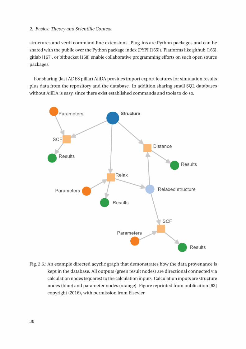
2. Basics: Theory and Scientific Context
structures and verdi command line extensions. Plug-ins are Python packages and can be
shared with the public over the Python package index (PYPI [165]). Platforms like github [166],
gitlab [167], or bitbucket [168] enable collaborative programming efforts on such open source
packages.
For sharing (last ADES pillar) AiiDA provides import export features for simulation results
plus data from the repository and the database. In addition sharing small SQL databases
without AiiDA is easy, since there exist established commands and tools to do so.
Fig. 2.6.: An example directed acyclic graph that demonstrates how the data provenance is
kept in the database. All outputs (green result nodes) are directional connected via
calculation nodes (squares) to the calculation inputs. Calculation inputs are structure
nodes (blue) and parameter nodes (orange). Figure reprinted from publication [63]
copyright (2016), with permission from Elsevier.
30

2.7. The AiiDA framework
2.7.1. Plug-ins in AiiDA
Data structures and file formats of different programs differ a lot. In order to cope with this en-
vironment in computational science, AiiDA has a slim base core code and everything around
it is organized in plug-ins, or apps. Plug-ins are designed, implemented and maintained
by the individual developers in the community. Otherwise maintaining, updating and bug
fixing all these individual interfaces would be impossible for a single scientific group. The
AiiDA team provides templates for scheduler, command line, data, parser, workflows and
calculation plug-ins. Besides these, also plug-ins for different storage back ends like other
database software as PostgreSQL and object stores can be implemented.
In order to deploy a program with AiiDA at least a calculation plug-in and a parser plug-in
have to be implemented. Parser plug-ins contain parsers for conversion of information from
input/output files into data structures. These data structures are stored in the database. Calcu-
lation plug-ins tell AiiDA how to launch a calculation for the given code, i.e., how to create the
needed code input from given data structures. Since there are several interfaces from external
community standards (cif [169], VESTA file formats [170], .xsf XCrySDen file format [171],
jmol, VASP input poscar, ASE and pymatgen structure objects) to basic AiiDA data structures,
it is convenient to work with the already implemented data structures whenever possible.
Though sometimes it is necessary, due to individual code requirements, to implement new
data structures for AiiDA which are code or community specific. This is achieved through a
data plug-in. Together all plug-ins and utility collection for a given program form an AiiDA
extension package. In recent years such packages have been implemented for several well
known electronic structure quantum engines (the Quantum Espresso package, VASP, FLEUR,
Yambo, Siesta, Castep, CP2K, KKR, Lammps, nwchem, phonopy, wannier90, ... ). The creation
of the package for the FLEUR code is part of this work.
AiiDA itself is a rather general framework and not at all limited to material science. It
just evolved out of the material science and electronic structure community. All extension
package names are collected in the aiida-registry [172], which accounts for AiiDA extension
name reservation to avoid collisions. From the registry AiiDA users are provided with a list
of available plug-ins (24 in 2018), their content, how they can be installed and if they are
compatible with each other in terms of requirements. On top of the registry it is straight
forward to build an app store or software manager functionality in the future.
2.7.2. Scientific Workflows (Workchains) in AiiDA
A very powerful feature of the AiiDA framework is the ability to write, run and share workflows.
AiiDA workflows/workchains are a way to automatically launch time consuming calculations
31

2. Basics: Theory and Scientific Context
that logically depend on each other without the user having to wait for each of them. The
workflow developer can encode expert knowledge. AiiDA provides the developer with tools to
ensure the provenance of data and logic. Workflows are very powerful protocols. Complex se-
ries of calculations can be launched through them with a small piece of Python code. In AiiDA,
workflows can be submitted to the daemon (run in the background) or executed with ‘run‘ in
the Python interpreter, blocking it throughout the whole workflow execution. AiiDA workflows
can be made robust and fault tolerant. They allow for seamless integration of knowledge from
others with Python. Anyone, also non expert users may deploy them. Workflows become
more than advanced bash scripts. They can include expert knowledge about how calculations
should be run and converged, reasonable parameters, optimal resource usage, automatic
error treatment and restarts. Workflows can expose simple interfaces with optimized default
values allowing deployment by non experts. Technically workflows are Python classes which
inherit from an AiiDA API base workflow class (WorkChain, WorkFunction). This allows the
workflow developer to use Python code and any packages he desires within the workflow. This
freedom may be an advantage of AiiDA over other workflow capable frameworks.
1 from aiida.orm import WorkflowFactory, load_group, Code
2 from aiida.work.launch import submit
3 fleur_eos = WorkflowFactory(’fleur.eos’)
4
5 inpgen = Code.get_from_string(’inpgen@otherhost’)
6 fleur = Code.get_from_string(’fleur@cluster’)
7
8 # presorted
9 crystal_strucs = load_group(label=’oqmd_strucs’).nodes.dbnodes
10 flapw_paras = load_group(label=’oqmd_paras’).nodes.dbnodes
11
12 for i,struc in enumerate(crystal_strucs):
13 res = submit(fleur_eos, structure=struc,
14 calc_parameter=flapw_paras[i],
15 fleur=fleur, inpgen=inpgen)
Code Listing 2.1: Small Python code snippet to launch workflows for a set of crystal
structures. This naive but powerful code example spawns a FLEUR
equation of states workflow for each structure in the Open Quantum
Materials Database (OQMD) resulting in over 8 million jobs to be managed
by AiiDA in this case. These jobs will have different computation demand
and may require different convergence strategies.
The example Python code in Code Listing 2.1 demonstrates how simple it becomes with AiiDA
to launch a high-throughput project. Beforehand all structures (more than 800,000 entries)
from the Open Quantum Materials Database (OQMD) [55] were imported into an AiiDA
database. Then for each crystal structure a node with several specific FLAPW parameters
32

2.7. The AiiDA framework
was prepared. With this node some parameters are specifically adjusted beyond the FLEUR
defaults. The launched workflow in this example could be interchanged with any other
workflow exposing a similar Python interface. Furthermore, the code and the machine to
run on plus optionally some maximum resources per job among other options have to be
specified. With a simple ‘for-loop‘ the user would launch in this code example an equation of
states workflow for every crystal structure in the OQMD. This would result in over 8 million
DFT self-consistency cycles submitted to some computing resource (in this case ‘cluster‘)
and managed by AiiDA. The code piece will execute quite fast (hours to days, depending on
the workstation and database speed), but the managed resulting computing jobs of these
spawned calculations will take over 10 years on a resource with a throughput of order two
thousand jobs per day. It is obvious that this naive demonstrative example will probably result
in a very high failure rate. A realistic high-throughput project has to be handled more carefully
and more verbosely. Only if the error rate of the infrastructure and the software environment
is sufficiently low, the throughput can scale up. It may also be necessary to split the project
into smaller parts, to predict plus control the work load and to understand if the deployed
quantum engine together with the workflows are robust enough for the project.
2.7.3. The AiiDA Community and the Python Universe
Keeping expert knowledge of the previous generation of scientists available in an adjustable
individual high-level work environment is key to longterm progress and knowledge accumu-
lation. AiiDA addresses this goal with its plug-in infrastructure and connectivity to any other
Python tool. Why work with Python? Python is one of the world’s most popular high-level
programming languages today, which allows for very fast development. The Python package
system allows for easy installation of software from the Internet through central servers like
PyPI [165] and package managers like Pip [173]. The Python community developed advanced
tools for writing (sphinx [174]) and hosting code documentation (Readthedocs [175]), style
checking (Pylint [176]), unit testing (unittest from the python standard library or pytest [177]),
debugging and notebook analysis (Ipython, Jupyter). Because of these capabilities and be-
cause Python is rather easy to learn, most software from the material informatics, data science
and machine learning communities is written in Python or at least comes with a Python
interface. Popular repositories useful for material science (and deployed within this work) are
among many others Pymatgen [152], Atomic simulation environment (ASE) [64], Spglib [178],
Matminer [179] and Seekpath [180]. Overall, with notebooks (like Jupyter-notebooks [181],
Beaker [182], Apache Zeppelin [183]) one does not have to migrate completely to Python,
since notebooks are capable of running all kinds of programming languages (not at peak
performance) in their code cells. For interactive data visualization in the browser Java-script
33

2. Basics: Theory and Scientific Context
libraries are often preferable over Python. The developer of a complex scientific workflow
can profit and build on the previous work in the community. Thus it is essential to be able to
use any Python code or package inside a workflow. This freedom plus throughput scalability
makes workflow engines like AiiDA or ASE more powerful compared to other, often graphical
workflow tools or extensions with their own implementations like UNICORE [184–186], JuBE
[187, 188], Kepler [189], pyiron [190] or others.
2.8. Machine Learning in Material Science
Machine learning in general is a useful toolbox to gain insight on data where the underlying
correlations and rules [191–195] are unknown. If one has an analytic expression, rule or
algorithm of a problem to produce the data and can apply it on the scale needed, it would not
make sense to apply machine learning on this problem. Still in electronic structure theory,
since calculations of larger systems are expensive or even impossible, it might make sense to
train some machine learning model to predict certain results instead of running expensive ab
initio simulation. This is especially the case for physical properties which depend only on
the local environment in the system, because here the cost for the application of a machine
prediction can be expected to scale with O (N ), where N is the system size. Finding a good
model or training a model might scale differently, depending on the algorithms.
Beyond this, machine learning methods are of course very helpful to extract knowledge
from high-dimensional data, that our community faces [40, 50, 55, 60, 196–198] from theory
and experiments. Experimental data is often rather scarce. Various machine learning stories
in material science include: Predicting if a structure is a metal or insulator [199], mechanical
properties [199, 200], glass formation [201], predicting crystal structures [31, 32, 148, 149,
202, 203], predicting stability [32, 200, 204], predicting nuclear magnetic resonance (NMR)
chemical shifts [205, 206], thermoelectrics [24], critical temperatures of superconductors [26]
or let the machine learning community on kaggle work on it like in the case of predicting
transparent oxides [207]. Also research groups worldwide advancing software packages
around machine learning specialized for material science like matminer [179].
Overall it is apparent that before knowledge can be extracted or helpful tools can be built
there needs to be a large enough volume of high-quality curated data. Within this work tools
and ways are laid out how this goal of generating larger data bases of high-quality all-electron
data from ab initio methods might be accomplished. For example, with a large enough and
diverse data set of core-level shifts, the prediction of chemical shifts of large structures and
layered systems may become feasible.
34

2.9. X-ray Photoelectron Spectroscopy (XPS)
2.9. X-ray Photoelectron Spectroscopy (XPS)
Photoemission spectroscopy (PES), where X-ray photoelectron spectroscopy (XPS) is a special
form of, is based upon the photoelectric effect discovered in 1887 by H. Hertz [208] and
theoretically explained by Einstein in 1905 [209]. Photons interacting with atoms can cause
electrons to be emitted where the kinetic energy of these photo-electrons is given by:
Ekin = hv −EB −ΦB, (2.32)
where hv is the energy of the incoming photon which gets lessened by the binding energy
EB of the electron and the work function ΦB, which accounts for the energy needed of an
photoelectron to leave the sample. The work function depends on the material and may also
have an angle and surface dependence.
EF = 0
Evac∞
EB
ΦAΦB
EkinA
hv EkinBE
Egap
Fig. 2.7.: Visualization of the energy levels in the photoemission process of a sample B and an
analyzer A. The energy level of a free electron E∞vac is per definition aligned between
the analyzer and the sample. If the Fermi energy EF of the detector aligns with
the Fermi energy of the sample through electrical contact, the binding energy EB
depends only on ΦA and E Akin. For materials with an energy gap at the Fermi energy,
measurements and simulations of binding energies are more challenging. (Figure
motivated by [210].)
In Fig. 2.7 the relevant energy level of the photoemission process are shown for a sample B
and an analyzer A. The energy level of a free electron E∞vac is per definition aligned between the
35

2. Basics: Theory and Scientific Context
analyzer and the sample. The binding energy, EB, is measured in reference to the Fermi energy
EF. As long as the work function of the spectrometer ΦA is larger then the work function of
the sample ΦB and the Fermi energy EF of the detector aligns with the Fermi energy of the
sample through electrical contact, the binding energy EB becomes EB = hv −E Akin −ΦA and
thus independent of the work function ΦB of the sample. For non-metals the Fermi energy
reference may pose a challenge [210] since impurities and charing effects change the Fermi
energy reference within the band gap Egap.
While photoemission is a charged excitation process there exist also a variety of neutral
excitation processes. Depending on the application several photoemission spectroscopy
techniques have been developed: ultra-violet spectroscopy (UPS) for valence band spectra,
angle-resolved photoemission (ARPES) for band structures measurements and others [76,
211].
The detailed quantum-mechanical description of general photoemission is complex, be-
cause the photoemission process involves the excitation of electrons in matter up to ionization
via the interaction with photons. These excited electrons have to leave the sample in order to
be detected by a detector, making electron transport play an important role in the process.
The photoelectrons and their corresponding core-holes in the solid with lifetimes of femto
seconds trigger a response from the electronic system, leading to so called ’final-state’ effects.
Final-state effects and energy loss features include core-hole screening effects, charge trans-
fer, plasmon excitations leading to additional rather broad peak structures, other relaxation
processes leading to satellite peaks, variable cross sections, different core-level-line inten-
sity ratios and lifetime effects like Coster-Kronig [212, 213]), shake-up and shake-off of the
valence electrons might lead to asymmetric peak shapes, background or additional peaks.
Screening effects might lead to additional splittings (multiplet-splittings) of core-level lines,
especially for magnetic systems. Contributions from Auger processes are also seen in XPS
spectra. A complete description of all this is essentially a time-dependent quantum many-
body problem which requires the inclusion of classical or quantum electro dynamics terms.
Other X-ray scattering processes contribute to the spectral background. In the literature are
several approximations to the photoemission process introduced. The sudden approximation
[214, 215] assumes that the primary excitation happens sudden relative to the adjusting of
the electron cloud, from this certain matrix element can be neglected. Depending on the
level of the approximation there is the one-step [216], or the three-step model [217, 218] of
photoemission. Initial-state approximations use ground state properties of the system and
neglect final-state effects. It is beyond the scope and interest of this thesis to cover the theory
of photoemission in detail, the interested reader is referred to [76, 210, 219, 220]. For the
core-level shifts of binary metals we used an initial-state approximation.
36

2.9. X-ray Photoelectron Spectroscopy (XPS)
Fig. 2.8.: Schematic single particle view of photoemission spectroscopy (figure from [75]),
showing how the density of states corresponds approximately to a measured spec-
trum. Electrons from the sample with a certain binding energy are excited by photons
with sufficiently high energy hν into the vacuum and measured by the analyzer. Core
electrons from the sample correspond to sharp peaks in the measured spectrum.
A simple schematic of photoemission spectroscopy is shown in Fig. 2.8. Exciting core
electrons result in rather narrow peak structures while excitations from the continuous valence
states will lead to a more continuous structure in the measured spectrum. The response of
valence electrons does not correspond simply to the density of states of the system. Since the
focus of this work lies on the chemical interpretation of high-resolution X-ray photoemission
spectroscopy of electronic core-level states, we restrict ourself to core-level XPS.
X-ray photoelectron spectroscopy (XPS) also known as electron spectroscopy for chemical
analysis (ESCA) is a well known spectroscopy technique for chemical analysis developed since
the 1960s. It is in widespread use in research and industrial applications 6 [75–77, 221]. XPS is
6User list of SDP software in 2004 https://www.xpsdata.com/user_list_2004.htm,
wikipedia https://en.wikipedia.org/wiki/X-ray_photoelectron_spectroscopy,
37

2. Basics: Theory and Scientific Context
applied to measure the empirical formula, the electronic state and chemical state of elements
contained within the surface area of a sample. The surface sensitivity, originates from the
fact that the mean free path of electrons in a material is 1 to 10 nm [222–225], which limits
the information depth. The penetration depth of X-ray photons with an energy of 1.5 keV is
about 1 to 10μm [226]. Compared to XPS other surface science methods like X-ray diffraction
(XRD) or Rutherford backscattering (RBS) have a 100-1000 fold deeper information depth of
several μm. A collection of surface science spectroscopy and microscopy methods is found in
[76]. While the extraction of the empirical formula from XPS is most of the time rather straight
forward, the chemical interpretation of high-resolution XPS data is often a challenge [78].
The different intensities of the core-electron lines arise strongly from the elemental and
orbital depended photoelectron cross-sections. H and He are not directly detectable by XPS,
because of their small cross-section for the energies of common X-ray sources. Depending on
the chemical environment of the element the core-level peaks shift in their binding energy.
These shifts are called chemical shifts, or core-level shifts (CLS) and are of interest because
they allow for a chemical interpretation of the system. Chemical shifts do not corresponds to
a simple picture of transfered charge between elements due to differences in electronegativity
[210].
For an XPS measurement usually ultra-high vacuum (< 10−9 mbar) is required to reduce
scattering events of electrons with gas particles. In addition, the surface should be fairly
empty of adsorbates which might influence the results. Nowadays, there are first ambient
pressure XPS systems for some use cases on the market [227, 228]. In Fig. 2.9 the schematic
setup of an XPS experiement is shown plus a photograph of a ultra-high vacuum setup for
XPS analysis from the IEK-4 of the Forschungszentrum Jülich. From a monochromatic X-ray
source photons with energy E = hv (for an Al-Kα source E =1486.6 eV, FWHM 0.1 eV) hit
the sample under a certain angle ψ. The analyzer collects only electrons exiting the sample
at angle Φ within a maximum entrance angle αmax and with a kinetic energy according to
the photoelectric effect of equation 2.32. The binding energy axis is usually calibrated by
measuring and aligning the Au-4f, Ag-3d, Cu-2p, Cu-3p peaks or other narrow known high
intensity lines. Through this the work function of the spectrometer (Eq. 2.32) is effectively
calibrated out, i.e. set to zero. The analyzer samples the energy of the electrons, by reducing
Ekin with an internal applied electric field that only electrons with the pass energy Epass
are counted at the detector. The setup in the IEK-4 uses a monochromatic aluminium Kα
radiation source MX 650 from VG Scienta and a half spherical analyzer from Scienta (R4000
user list CasaXPS http://www.casaxps.com/links/academic_site_licenses.htm
38

2.9. X-ray Photoelectron Spectroscopy (XPS)
L2), with an energy resolution as a function of the pass energy [230]
ΔE =(
w
a +b+ α2
max
4
)Epass (2.33)
where w is the width of the entrance aperture, αmax the entrance angle and a, b are the inner
and outer radii of the analyzer. From this arises a trade-off between resolution and signal
intensity. The highest practical energy resolution of such a system lies around 0.2 eV for
XPS [230]. The resolution also becomes limited by the natural line width of about 0.16 eV of
the Al-Kα line [231]. With higher quality and intensity of monochromatic light sources like
synchrotron radiation the resolution can be better.
39
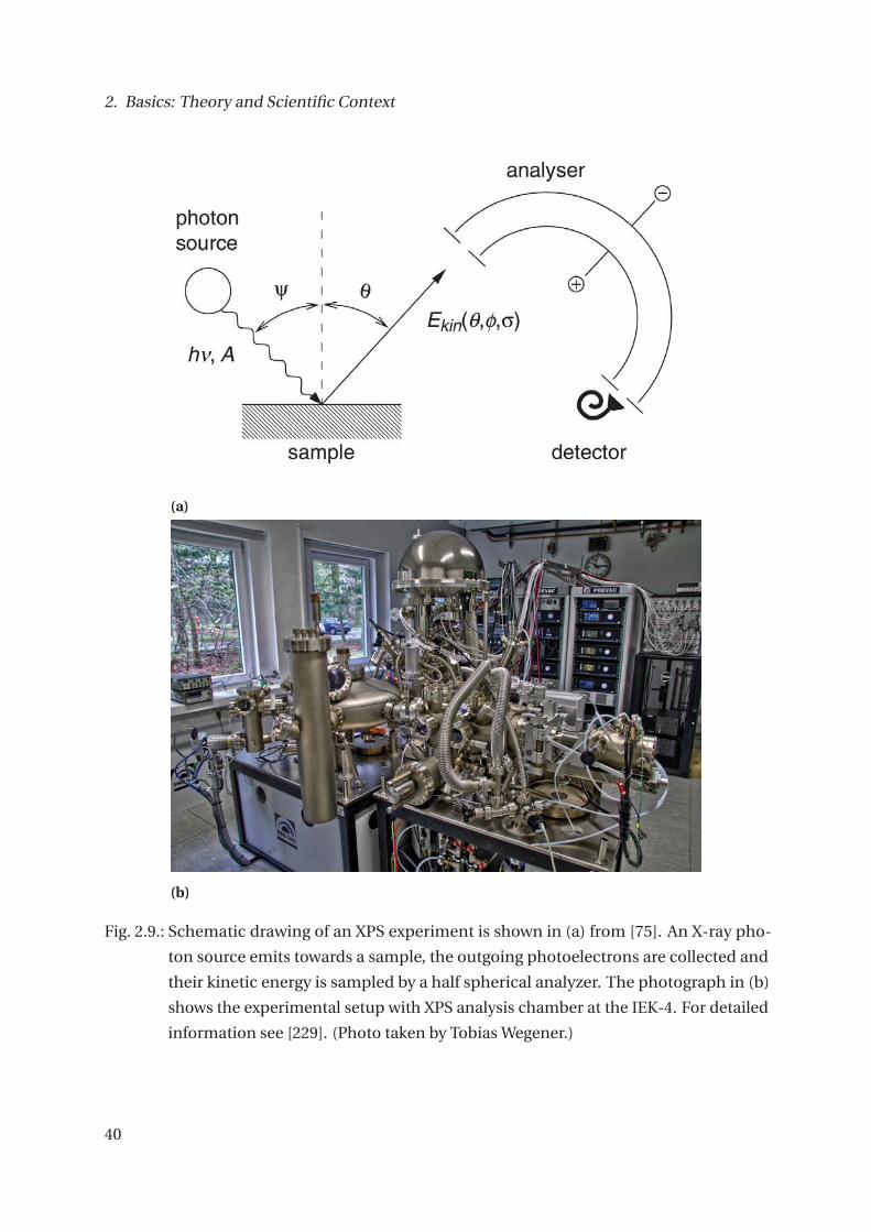
2. Basics: Theory and Scientific Context
(a)
(b)
Fig. 2.9.: Schematic drawing of an XPS experiment is shown in (a) from [75]. An X-ray pho-
ton source emits towards a sample, the outgoing photoelectrons are collected and
their kinetic energy is sampled by a half spherical analyzer. The photograph in (b)
shows the experimental setup with XPS analysis chamber at the IEK-4. For detailed
information see [229]. (Photo taken by Tobias Wegener.)
40

2.9. X-ray Photoelectron Spectroscopy (XPS)
2.9.1. Current Chemical Interpretation of XPS
Different information on a sample is obtainable from XPS spectra. While information of the
elements present and their quantity is rather straight forward from a survey XPS spectrum,
a detailed chemical interpretation of the exact phase content from a high-resolution XPS
spectrum is still a challenge. Usually, in order to do so a multi-peak-function fit including a
background function which best approximates the spectral data has to be found first. The
fit results may depend on the scientist fitting the spectrum and on his experience [232, 233].
Also it makes a difference if the spectral background fit is adjusted consistently in the fitting
procedure [234].
The fit is conducted with statistical methods like least squares, maximum likelihood or
others. Notice, that a fit does not correspond to a deconvolution of the spectrum. Finding
a good fitting curve is usually not a challenge, while the interpretation of the fit can be
hard or the fit may even be unphysical. A variety of standard tools exist to help with the
mathematical fitting and justification, among others UniFit [234, 235], CasaXPS [236], SDP
[237] and MultiPak [238]. Often Voigt profiles are chosen as peak functions, but in some
cases fitting with asymmetric peak functions is necessary. Voigt profiles (Eq. 2.34) are a
convolution of a Lorentzian and a Gaussian (Eq. 2.35). The Lorentzian part originates from
the usual excitation shape of a process decaying exponential in time from Fermis golden rule
[239, 240] broadened by the finite lifetime of core-holes. The Gaussian part accounts for all
contributions of additional broadening effects. Broadening effects arise from the natural
line-width of the monochromatic photon source (~0.16 eV) [231], the energy resolution of the
analyzer, vibrational effects and other sources [218].
V (x,μ, fG, fL) =G(x −μ, fG)�L(x, fL) =∫∞
−∞G(x ′ −μ, fG) ·L(x −x ′, fL)d x ′ (2.34)
where the Gaussian G and Lorentzian L are given by
G(x −μ, fG) = 1
fG�
2πe
(x−μ)2
2 f 2G , L(x, fL) = fL
π((x)2+ f 2L )
(2.35)
A Voigt profile V (x,μ, fG, fL) (Eq. 2.34) has three free parameters, the position μ, Lorentzian
broadening fL and the Gaussian broadening fG. The area under a Voigt profile is normalized
to one.
When fitting XPS spectra for a certain binding energy region with several Voigt profiles the
Lorentzian broadening fL and the Gaussian broadening fG can often be kept the same for all
profiles and varied as two fit parameters. Additional the profile positions are optimized each
and the area under each peak, which translates into fitting the peak height in most routines. In
41

2. Basics: Theory and Scientific Context
total this amounts to Nfit = 2+2 ·N fit parameters for N Voigt profiles. When fitting multiplets,
like 4 f5/2 and 4 f7/2 states, constraints on the peak positions can be built into the fit due to an
assumed constant peak splitting and on the peak areas by fixing area ratios. Therefore, to fit
doublets more peak functions (N) are needed but the number of total fit parameter required
reduces to Nfit = 2+N with the assumptions above. In the case of asymmetric peak shapes
additional fit parameters for the asymmetry of the peak function are introduced. Asymmetric
peak shapes arise from valence band shake-offs. The theoretical asymmetric form of a main
line peak was investigates by Doniach and Sunjic [220]:
DS(x −μ,α, fd) =cos
[πα2 + (1−α)arctan
(x−μ
fd
)](
f 2d + (x −μ)2
) (1−α)2
, (2.36)
where μ is the position of the main line, fd is a broadening parameter and α tunes the
asymmetry. For α= 0 the Doniach-Sunjic (DS) shape becomes a Lorentzian. Notice, that the
peak maximum of the DS shape is not exactly at μ and depends on α [220]:
(x −μ)DS, max = fd cot(π
2−α). (2.37)
The tail of this profile is non-zero for energies far away from the main line, making the profiles
area infinite. This leads to fitting problems, since the tail contribution of this form has to be
adjusted with the background.
To overcome this problem, other asymmetric peak shapes with finite areas are introduced.
A commonly applied [78, 241] shape is an asymmetric Lorentzian convoluted with a Gaussian
(LA):
L A(x,μ, fL, fG,β,α) =G(x, fG)� AL(x −μ, fL,β,α) (2.38)
AL(x −μ, fL,α,β) =⎧⎨⎩
[L(x −μ, fL)]α x ≤μ,α≥ 1.0
[L(x −μ, fL)]β x >μ,β≥ 1.0(2.39)
L(x −μ, fL) = 1
4(
x−μfL
)2 +1(2.40)
where α and β (≥ 1.0) are parameters for the asymmetric form of the Lorentzian L(x −μ, fL)
of height one at position μ with a full-width half-maximum fL. The fixed height ensures the
continuity of the AL function. The AL peak shape is fitted with three to four parameters and
has a similar tail as the DS profile, but with a finite area. For curve fitting of transition metal
peaks the asymmetric Lorentzian (AL) is convoluted with a Gaussian G(x, fG) with FWHM fG
forming the LA peak shape.
For the background of a spectrum the most commonly used fit functions are the Shirley
[242, 243] and the Tougaard background [244, 245] functions, also a linear background or
42

2.9. X-ray Photoelectron Spectroscopy (XPS)
Fig. 2.10.: This figure showns the result of a common fitting procedure. Three Voigt profiles
had to be included in order to achieve good agreement with the data points. For the
background estimation the Shirely method was applied. The data and fit performed
with UniFit are taken with permission of the author from [229].
others functions are sometimes applied [246]. The iterative Shirley background is a special
type of Tougaard background and has the form [243]:
Si(E) = k∫∞
E( j (E ′)−Si−1(E ′)dE ′ (2.41)
where Si(E) is the background at iteration step i and energy E, k is a constant and j (E ′) is the
measured spectrum corrected by other non inelastic loss effects. The initial background S0 is
assumed to be a constant.
An example fit to an experimental XPS spectrum with three Voigt profiles and a Shirley
background is shown in Fig. 2.10.
After a successful fit has been found, the fit results have to be interpreted. For the interpre-
tation the positions of the individual peaks have to be related to known positions of possible
phases in literature or reference single crystal spectra. This part often fails for several reasons.
First, literature data is scarce. The NIST XPS database [90] contains entries for around 6,300
systems, of which 3,000 are oxides and 2,700 contain carbon. The NIST database provides
43

2. Basics: Theory and Scientific Context
Fig. 2.11.: Interpreted XPS spectra of an Fe-O system with asymmetric peak shapes from
Biesinger et al. [78] investigating Fe-based nano particles on a glass substrate. The
interpretation was done by fitting Fe-O phases and reusing their fit parameters
for mixed systems. This evaluation represents the state of the art. The figure is
reprinted from publication [78] copyright (2010), with permission from Elsevier.
28,000 binding energies of which 15,700 are unique plus 7,500 unique core-level shifts. There
are other sources for data reviewed by B. Crist in [247], which includes a licensed database
with 70,000 non-unique spectra [237] and books [226]. Second, in order for literature data to
be accurate enough the energy scales have to be calibrated carefully and other information
of the X-ray source and analyzer (resolution, uncertainties) needs to be available. If this is
not the case or unclear, it leads to large uncertainties and spread in the data [248]. Third,
other effects in XPS spectra need to be accounted for before the fitting procedure or within
it like including known satellite positions, plasmons, or other spectral contributions. If the
investigated sample was not a metal, it may be necessary to correct the energy scale for
charging effects of the sample. Additional data from other surface science methods, like XRD,
may support and constrain the spectrum interpretation. Overall, this chemical evaluation
way is probably fundamentally limited and only applicable to the simplest material phases.
The fundamental limitation arises in detail from the fact that the sum of two (peak) localized
functions at different energies lies not in the same (peak) function space. The sum of each
unique chemical environment contributes with a different intensity weight to the spectrum.
44
2.9. X-ray Photoelectron Spectroscopy (XPS)
This makes a fitting with no assumption approach nearly arbitrary for materials (mixtures)
with several chemical environments close by. Also binding energies and therefore also binding
energy shifts are not unique, since similar chemical environments of an element can exist
in different materials. For molecules it is known that sometimes the different C 1s core-level
shifts are identifiable by their separated positions and their intensities [249, 250].
With the help of experimental high-resolution reference spectra for certain pure phases it is
also partially possible to determine not only phases present but also relative amounts of each
phase as demonstrated in [78] for first row transition metals, oxides and hydroxides of Cr, Mn,
Fe, Co and Ni. Such a spectrum from the work of Biesinger et al. is shown in Fig. 2.11. Fitting
spectra with such complexities is state of the art.
It is known from [251] that satellite positions and intensities do not have to be the same
for different chemical environments of the same element. Though it is possible to calculate
satellite positions and intensities from ab initio [252] or cluster model calculations [251].
Overall, it should be clear that a in detail full chemical interpretation of high-resolution XPS
spectra of complex systems is hard and leads often to incomplete evaluations and guesses. A
different approach for the chemical analysis of XPS driven by ab initio data is discussed in
section 3.2.
2.9.2. Quantities for XPS from ab initio Simulations
It has been pointed out above that absolute core-level binding energies (BE) and their chemi-
cal shifts (CLS), not to be confused with chemical shifts of nuclear magnetic resonances, are
valuable for understanding the chemistry of a system. Through the shifts in binding energy
chemical phases can be identified. Literature CLS data for materials systems are often rare,
and experiments to produce reference data are expensive and time consuming. Without refer-
ence data the phases can hardly be identified, making this a kind of chicken and egg problem
for complex materials. The data issue could be solved with first principles methods through
high-fidelity workflows, by performing high-throughput calculations on every material of
interest and deploying machine learning beyond that.
The calculated chemical shifts and binding energies for chemical interpretation need to
have a comparable total accuracy of ≈0.1 eV to experiments. Furthermore, the predictions
of doublet and multiplet splittings needs to be very exact ≈0.01 eV in order to be useful for
fitting and comparing with experiments.
To calculate core-level shifts one needs a method treating all-electrons, including the core
electrons, or at least the electrons for the main core-level line of interest. Other approxi-
mations for non all-electron methods like the Z+1 [253] approximation or frozen core are
not precise enough for core-level shifts [210]. In chemistry and solid state physics scientists
45

2. Basics: Theory and Scientific Context
have worked on predicting these values and photoemission spectra since the availability of
high-resolution XPS measurements [210, 254, 255].
Focusing on ab initio methods, there are several methods capable of doing so, with growing
computationally hardness as they include more physics and effects of the many-body system
(’final state’ effects). To save computing resources one wants to use the cheapest method
within its scope of application and then climb up the ladder of complexity if necessary.
2.9.2.1. Initial-state Approximation
A rather simple way to calculate core-level shifts (ΔEB,n� j ) is by comparing the Kohn-Sham
energies with respect to the Fermi energy of a standard DFT self-consistent-field ground-state
calculation of a system (2) with the respective Kohn-Sham energy in the elemental reference
system (1).
ΔEB,n� j = ε1,n� j −ε2,n� j (2.42)
where ε1,n� j is the Kohn-Sham energy of an atom-type in system 1 of the core-state specified
by the quantum numbers n,�, j or other quantum numbers in the full relativistic case with
orbital moment and crystal field. Since system 1 and reference system 2 are both in the ground
state, this corresponds to an initial-state approximation, neglecting any final-states effects..
This approximation is expected to work for metals as the Fermi energy can be determined
and for a grounded sample the reference energy for binding energies in experiments is also
the Fermi energy. This approach is reported to be used by several ab initio programs [210,
255, 256]. For non-metal systems this approach is expected to give only good results for the
relative shifts between different atom-types in the structure since the reference energy is the
same. Finding a global reference energy between different phases and to experiment is a
challenge here. Also any final-state influences are not included in this approximation.
Influences of FLAPW parameters on Kohn-Sham core-level energies for theFLEUR program
have been investigated in [257] (section 3.1.3 ’Core Level Dependencies’ and section 3.1.4).
There it was pointed out that the Kohn-Sham energies converge before the charge density is
converged and that they depend substantially on the muffin-tin radius and the basis cutoffs.
The dependence on the muffin-tin radius varies for individual core levels but this variation
can be minimized by calculating with enough (>900) grid points within the muffin-tin spheres.
Spin-orbit coupling leads to a constant shift in the Kohn-Sham core-level energies. In contrast
a slight increase in cell volume within a ±2 % range has a linear dependence on the Kohn-
Sham energies of 100 meV per percent volume change. In [257] it was concluded that the
core-level shifts can be converged with respect to the FLAPW parameters within an accuracy
below 100 meV, making them comparable to experiments. For this accuracy it is best to
choose the same muffin-tin parameters for an element. This was shown for the W 4f core
46

2.9. X-ray Photoelectron Spectroscopy (XPS)
levels of the Be2W system. Inclusion of spin-orbit coupling lead to a 1%, 10 meV offset for
the 4f core-level shifts of W. These findings allow for automation of accurate core-level shift
calculations on different structures.
In [132, 258] it was shown that dependencies on the muffin-tin radii can be further re-
duced by modifying the FLAPW basis set and including more higher local orbitals. This also
decreased dependencies of Kohn-Sham energies. It was confirmed for several systems and
different core-levels that their core-level shifts can be converged to high accuracy with the
FLAPW basis set and independent of FLAPW parameters, if they are the same and reasonable.
2.9.2.2. Binding energies from Core-hole Calculations
Kohn-Sham energies themselves are far off from experimental binding energies and not
directly comparable. Absolute binding energies can be calculated with standard DFT via a
core-hole calculation. The electronic structure can be relaxed within the presence of core-
hole to mimic the ’final state’. Such a core-hole can be calculated as a neutral excitation, i.e.
placing the electron in the valence band, or the electron is removed leaving a charged system.
To account for induced magnetism of a core-hole, a spin-polarized calculation should be
performed. The response to the core-hole accounts for some screening effects of the electron
cloud. The binding energy EB,i,n� j is calculated as the difference of total energies of systems
with a core-hole Etot,1,ch and without Etot,1.
EB,i,n� j = Etot,1 −Etot,1,ch (2.43)
From the difference of binding energies (EB,1,EB,2) a chemical shift ΔEB,n� j can again be
estimated.
ΔEB,n� j = EB,1 −EB,2 (2.44)
These calculations are computational more demanding as for the FLEUR program they
require super-cell setups in order to converge the binging energies. This is so because the
results depends on the number electrons available for the screening, i.e the core-hole impurity
density should be small. In order for the core-level shifts to be on the same accuracy level,
the binding energies need also be as accurate as 100 meV. This approach is referred to in the
literature as ΔSC F .
Oxides, or insulators with a large bandgap are in general from a DFT point in various
ways harder to treat correctly. First, oxides come often in a rich phase space (>5 phases),
with different configurations, environments and disorder, oxides usually do not grow as
single crystals but in multiple configurations. This makes it hard in the first place to chose
what to calculate and to decide how to compare to experimental results. Second, oxides are
sometimes at the boundaries of applicability of standard DFT functionals, since the bandgap
47

2. Basics: Theory and Scientific Context
is underestimated and possible strong electron correlations are not accounted for correctly.
Calculating with advanced functionals or other methods make comparison of total energies
less rigorous. Longer core-hole lifetimes and hole-electron interactions in insulators lead to
possible significant excitation effects, matrix effects, final-state features in the spectra, which
need to be treated correctly in the method and are beyond standard ground-state DFT. High
quality XPS data of insulators are also experimentally harder to obtain, because of sample
charging effects which need to be accounted for in the right way. When comparing to theory
there is also the problem with the energy reference.
2.9.2.3. Beyond standard DFT and the FLEUR Program
Beyond the initial-state and core-hole calculation in standard DFT there exist various com-
putationally more demanding ab initio methods to calculate optical responses of a system
and time-dependent processes. They are especially required to describe the response of the
valence electrons to a strong perturbation or driving force more accurately. These methods
can to some extent predict the influence or importance of matrix elements. Most of these
methods are state of the art and currently applicable to systems smaller than 100 atoms since
have a scaling which is worth than cubical with the system size.
The GW-approximation (GW) [259] is a green function based method which includes
explicit many-body effects useful to retrieve response function like the spectral function,
or the dielectric function. Core-levels can also be included in GW and absolute binding
energies have been calculated within an accuracy of 0.3 eV in [260]. This accuracy might not
be accurate enough to compare to experiments.
In time-dependent density functional theory (TDFT) [261] processes can be calculated with
DFT over time, allowing for the calculation of processes like photoemission.
To describe the electronic response of neutral excitation more accurately one can solve the
Bethe–Salpeter equation (BSE) [262]. By this exciton peak positions, form and magnitude and
influence on the electronic structure can be predicted [263, 264], or whole X-ray absorbtion
spectra (XAS).
48

3. Method Development
3.1. The AiiDA-FLEUR Package . . . . . . . . . . . . . . . . . . . . . . . . . . . . . . . 49
3.1.1. Plug-in Layouts . . . . . . . . . . . . . . . . . . . . . . . . . . . . . . . . . . 50
3.1.2. Implemented Workflows for FLEUR . . . . . . . . . . . . . . . . . . . . . . 55
3.1.3. Core-level Spectra Turn-key Solution . . . . . . . . . . . . . . . . . . . . . 68
3.1.4. XPS Spectra Visualization App . . . . . . . . . . . . . . . . . . . . . . . . . 77
3.2. Fitting XPS Spectra from a Complete ab initio Dataset . . . . . . . . . . . . . . . 79
3.3. Method Development Sum-up . . . . . . . . . . . . . . . . . . . . . . . . . . . . . 84
Some selected results of the method development part of this work are presented in this
chapter. One section describes the AiiDA-FLEUR package, which connects the FLEUR code to
the AiiDA framework and the developed workflows and Python utilities. Another section deals
with the first implemented steps towards a full turn-key solution for the automatic evaluation
of well-behaved X-ray photoemission spectra from ab initio results.
3.1. The AiiDA-FLEUR Package
The AiiDA-FLEUR Python package1 enables the usage of the all-electron DFT code FLEUR
[79]) with the AiiDA framework [63, 156]. The package contains AiiDA plug-ins for the FLEUR
code itself, its input generator (inpgen) and a data structure representing the FLEUR input.
Furthermore, it contains workflows, property calculator protocols and utilities to create a
high-level work environment. The package contains over 6000 lines of Python code, is open
source under MIT license and is released on github and PyPI (the Python package index). The
package was developed as part of the MaX EU Center of Excellence [265] contribution from
the Forschungszentrum Jülich GmbH, (IAS-1/PGI-1), Germany. Since the development of
other Python packages for other juDFT codes2, AiiDA independent utilities were moved to
1Code: https://github.com/JuDFTteam/aiida-fleur
Documentation: https://aiida-fleur.readthedocs.io2https://github.com/JuDFTteam/
49

3. Method Development
the separate ’masci-tools’ (material science tools) repository3. This ensures the reusability
of file readers, utilities, visualizations and parsers for other purposes, tools and packages.
The AiiDA-FLEUR package ships with the plot function plot_fleur to quickly gain a default
visualization of any database node or nodes produced by FLEUR calculations or workflows.
Please note that the version of AiiDA-FLEUR (0.6.3) discussed within this work is compatible
with AiiDA versions <1.0, since most of the results of this work are produced with this version.
For AiiDA versions >1.0 the API is slightly different and AiiDA-FLEUR versions >1.0 have to be
used.
3.1.1. Plug-in Layouts
In the following subsections the two individual code plug-ins and the data plug-in of the
AiiDA-FLEUR package are presented in more detail. AiiDA calculation plug-ins, as fundamen-
tal building blocks, contain instructions on how to create valid input from information in
the database and what information to parse from output files and to store in the database.
Provenance direct acyclic graphs of data nodes and calculation nodes show what input nodes
are needed for a calculation and what output nodes are produced. The calculation plug-ins
form the basic building blocks of more complex AiiDA provenance graphs of workflows and a
whole provenance network of simulation data. Python code usage examples and details on
the output node contents in the database are presented additionally within this section.
3.1.1.1. FLEUR Input Generator Plug-in
The input generator plug-in is capable of running the FLEUR input generator (inpgen)
with most of its features. Features like crystal structure modification or creation are not
supported on purpose, because they would allow for breaking the data provenance. To
initialize a FleurinputgenCalculation it is enough to provide a StructureData node and a Code
node as shown in Fig. 3.1. From these inputs a FleurinputData object with default FLAPW
parameters will be created. Alternatively to the default FLAPW parameters one can provide
an additional ParameterData node as input with the corresponding parameters. A successful
FleurinputgenCalculation creates four output nodes in the database. The FleurinpData
node represents the input files for a FleurCalculation. The RemoteData node points to the
folder where the calculation was run and the Folder node points to a local folder like object
containing all the retrieved files from an inpgen run. Retrieved files include the FLEUR
input file ’inp.xml’, the inpgen output file ’out’, an ’shell.out’ file containing piped shell
output and an ’out.error’ file with the piped standard error stream.
3https://github.com/JuDFTteam/masci-tools
50

3.1. The AiiDA-FLEUR Package
Fig. 3.1.: Database input and output nodes in the directed acyclic provenance graph for a
single run of the input generator inpgen.
3.1.1.2. FLEUR Calculation Plug-in
The calculation plug-in for the FLEUR code allows for deployment of the code through AiiDA.
Fig. 3.2 shows a node graph of a FleurCalculation. Input nodes are a Code node, a Fleurin-
Fig. 3.2.: Database input and output nodes in the directed acyclic provenance graph for a
single run of the FLEUR code.
pData node and an optional RemoteData node from a previous parent FleurCalculation to
continue from its output results. In the ParameterData output node of a FleurCalculation
51

3. Method Development
basic calculation results are stored, for example the total energy, Fermi energy, band gap,
charge distance and meta data information of a single FLEUR run.
1 print(fleuroutputnode.get_dict())
2 {"bandgap": 0.0061037189, "bandgap_units": "eV",
3 "charge_den_xc_den_integral": −650.251477273, "charge_density1": 9.4019e−06,
4 "charge_density2": 9.5578e−06, "creator_name": "fleur 27",
5 "creator_target_architecture": "GEN", "creator_target_structure": " ",
6 "density_convergence_units": "me/bohr^3", "energy_valence_electrons": −4.20135128,
7 "end_date": {"date": "2018/08/08", "time": "09:47:40"}, "energy": −879603.931538445,
8 "energy_core_electrons": −19771.3543364295, "energy_hartree": −32324.8485355339,
9 "energy_hartree_units": "Htr", "energy_units": "eV",
10 "fermi_energy": 0.6050871733, "fermi_energy_units": "Htr", "force_largest": 0.0,
11 "magnetic_moment_units": "muBohr", "magnetic_moments": [0.0105619536, −0.0026848541],
12 "magnetic_spin_down_charges": [4.8629403112, 4.6137500971],
13 "magnetic_spin_up_charges": [4.8735022647, 4.611065243],
14 "number_of_atom_types": 2, "number_of_atoms": 2, "number_of_iterations": 26,
15 "number_of_iterations_total": 26, "number_of_kpoints": 156, "number_of_species": 1,
16 "number_of_spin_components": 2, "number_of_symmetries": 8,
17 "orbital_magnetic_moment_units": "muBohr", "orbital_magnetic_moments": [],
18 "orbital_magnetic_spin_down_charges": [], "orbital_magnetic_spin_up_charges": [],
19 "output_file_version": "0.27", "overall_charge_density": 1.88766e−05,
20 "parser_info": "AiiDA Fleur Parser v0.1", "parser_warnings": [],
21 "spin_density": 1.7792e−06, "start_date": {"date": "2018/08/08", "time": "09:46:17"},
22 "sum_of_eigenvalues": −19775.5556877095, "title": "A Fleur calculation with aiida",
23 "unparsed": [], "walltime": 83, "walltime_units": "seconds",
24 "warnings": {"debug": {}, "error": {}, "info": {}, "warning": {}}}
Code Listing 3.1: Database content of the ParameterData output node of a FleurCalculation.
The node is a dictionary contaning key value pairs. Unit information of
values are given by a seperate key with the same name plus a ’_units’ suffix.
In Code Listing 3.1 such parsed content of a ParameterData output node is shown. It contains
relevant meta information to understand what was going on in the simulations and should
answer the following questions: What system was calculated? Did the calculation succeed?
How far did it converge? How long did it take? Have warnings or errors of any kind occurred?
In certain run modes of FLEUR which change the crystal structure in the calculation, i.e., by
execution of relaxation steps, a FleurinpData node corresponding to the new input files with
the output crystal structure will be returned by a FleurCalculation.
Code Listing 3.2 presents a minimum Python code example to run a FleurinpgenCalculation
with a subsequent FleurCalculation. One has to import all relevant Python classes and
functions. AiiDA Factory methods allow for loading classes from their entry point names.
This way the user does not have to remember from where plug-in Python classes have to be
imported. All input nodes for the calculations have to be loaded from the database, which
were prepared beforehand. To launch a calculation the class and all the input nodes have to be
52
3.1. The AiiDA-FLEUR Package
1 from aiida.orm import load_node, Code, CalculationFactory
2 from aiida.work.launch import run
3
4 inpgen_calc = CalculationFactory(’fleur.inpgen’)
5 fleur_calc = CalculationFactory(’fleur.fleur’)
6
7 inpgen = Code.get_from_string(’inpgen@localhost’)
8 fleur = Code.get_from_string(’fleur@localhost’)
9
10 # prestored Structure and parameters
11 crystal_struc = load_node(<pk>)
12 flapw_para = load_node(<pk>)
13
14 res = run(inpgen_calc, structure=crystal_struc,
15 calc_parameter=flapw_para, inpgen=inpgen)
16
17 fleurinp = res.get(’fleurinp’, None)
18 res_fleur = run(fleur_calc, fleurinp=fleurinp, fleur=fleur)
Code Listing 3.2: Minimal Python code example to run the input generator and a follow
up FLEUR calculation. The crystal structure and FLAPW parameters are
loaded from the database in this case. Both calculations are executed with
’run’, thus blocking the Python interpreter.
parsed to the run or submit launcher functions. In this example the calculation is executed
in the Python interpreter with run in order to wait for the FleurinpgenCalculation to finish
before the FleurCalculation is executed.
3.1.1.3. Fleurinput Data Structure and Modifier
As a typical FLEUR calculation needs a significant amount of additional input parameters
beyond the crystal structure represented in AiiDA, functionalities to efficiently manage and
manipulate these inputs are wanted. For this the possibility to extend AiiDA by new data
structures [63] was utilized. The FleurinpData class was implemented, to represent FLEUR
input files and to provide user friendly methods for processing input or extracting information
from it. The input files are stored in the file repository while in the database a part of the
full inp.xml file is stored for query capabilities. The FleurinpModifier class ensures that
provenance is kept through all input modifications and allows for previews and undo of
changes. In order to be able to undo modifications, the class stores all change requests in a
queue. These change requests will only lead to a new FleurinpData data node if the freeze()
method is called.
General class methods of FleurinpModifier include:
• validate(): Test if the changes in the queue produce valid FLEUR input
• freeze(): Applies all the changes in the queue (calls the workfunction
53

3. Method Development
modify_fleurinpdata) and returns a new FleurinpData object
• changes(): Displays the current queue of changes
• show(display=True, validate=False): As a test applies the modifications and displays/prints
the resulting inp.xml file.
The following change methods have been implemented so far for the FleurinpModifier class
to ease input file manipulation, while others will follow in the future:
• xml_set_attribv_occ(xpathn, attributename, attribv, occ=[0], create=False): Set an at-
tribute of a specific occurance of xml elements.
• xml_set_first_attribv(xpathn, attributename, attribv, create=False): Set an attribute of
first occurance of an xml element.
• xml_set_all_attribv(xpathn, attributename, attribv, create=False): Set an attribute of
several xml elements.
• xml_set_text(xpathn, text, create=False): Set the text of first occurance of an xml element.
• xml_set_all_text(xpathn, text, create=False): Set the text of xml elements.
• create_tag(xpath, newelement, create=False): Insert an xml element in the xml tree.
• delete_att(xpath, attrib): Delete an attribute for xml elements from the xpath evaluation.
• delete_tag(xpath): Delete an xml element.
• replace_tag(xpath, newelement): Replace an xml element.
• set_species(species_name, attributedict, create=False): Specific user-friendly method to
change parameters of species.
• set_atomgr_att(attributedict, position=None, species=None,create=False): Specific method
to change atom group parameters.
• set_inpchanges(self, change_dict): Specific user-friendly method for easy changes of
attribute key-value type.
• set_nkpts(self, count, gamma=’F’): Specific method to set the number of k-points.
Python Code Listing 3.3 demonstrates how to initialize a FleurinpData object and how the
FLEUR input is changed without breaking the provenance by using the FleurinpModifier
class. In this example the kmax basis cutoff value is changed and the ’dos’ switch is set to ’True’.
This operation leaves three linked nodes in the database, a FleurinpModifier CalcFunction,
a returned new FleurinpData node and a generated ParameterData node with the applied
changes. Since FleurinpModifier queues the changes, all input modifications are reduced to
this minimal database footprint without spamming the database with uninteresting nodes.
54
3.1. The AiiDA-FLEUR Package
1 from aiida.orm import DataFactory
2 from aiida_fleur.data.fleurinpmodifier import FleurinpModifier
3 FleurinpData = DataFactory(’fleur.fleurinp’)
4
5 BeTi_inpxmlfile = ’./inp.xml’
6
7 F = FleurinpData(BeTi_inpxmlfile)
8 fm = FleurinpModifier(F)
9 fm.set_inpchanges({’dos’ : True, ’Kmax’: 3.9 })
10 fm.show() # display input file with changes
11 new_fleurinpdata = fm.freeze() # apply changes
Code Listing 3.3: Python code example to work with FleurinpData and modify input with
the FleurinpModifier class. This example initializes a FleurinpData node
and changes some parameters of a species, resulting in a new FleurinpData
node stored in the database.
3.1.2. Implemented Workflows for FLEUR
A powerful feature of the AiiDA framework is the ability to develop, run and share workflows
[63]. AiiDA workflows are a way to automatically launch time consuming calculations that
logically depend on each other without the user having to wait for each of them. The workflow
developer encodes expert knowledge and ensures the provenance of data and logic while
having access to the Python universe. The developer should try to keep the database footprint
(provenance overhead) as small as necessary for a high-throughput workflow. Workflows
are powerful property calculator protocols with complex series of calculations able to be
launched with a small snippet of Python code. Additional logic can be encoded in workflows
like how to best run and converge calculations, find reasonable parameter sets, determine
optimal computing resources, treat errors automatically and enable restarts.
The AiiDA-FLEUR package comes with a set of workflows. The basic ones converge a
FLEUR calculation, calculate a density of states, an electronic band structure or an equation
of state. AiiDA-FLEUR additionally contains more advanced workflows to manage core-hole
simulations and calculate core-level electron binding energy shifts. A typical run of the basic
FLEUR self-consistent field workflow creates about 20 database nodes and around 10 files
of different sizes to be stored permanently. Advanced workflows need a few to hundreds of
self-consistent field subworkflows.
55

3. Method Development
1 from aiida.orm import WorkflowFactory,load_group, Code, DataFactory
2 from aiida.work.launch import submit
3 ParameterData = DataFactory(’parameter’)
4 workflow_class = WorkflowFactory(’fleur.<wf entrypoint>’)
5
6 inpgen = Code.get_from_string(’inpgen@otherhost’)
7 fleur = Code.get_from_string(’fleur@cluster’)
8
9 strucs = load_group(label=’some_strucs’).nodes.dbnodes
10 calc_paras = load_group(label=’FLAPW_paras_for_strucs’).nodes.dbnodes
11
12 # example options node for a cluster running slurm
13 options = ParameterData(dict={
14 ’resources’ : {u’num_mpiprocs_per_machine’: 24, u’tot_num_mpiprocs’: 48},
15 ’max_wallclock_seconds’: 5*60*60, ’queue_name’ : ’’,
16 ’custom_scheduler_commands’ : u’#SBATCH −−partition=batch’,
17 ’environment_variables’: {’OMP_NUM_THREADS’ : ’1’}
18 })
19
20 # launch workflow for all structures
21 # with default workflow parameter since they are not specified in this case
22 for i,struc in enumerate(strucs):
23 res = submit(workflow_class, structure=struc, options=options,
24 calc_parameters=calc_paras[i], fleur=fleur, inpgen=inpgen)
Code Listing 3.4: Generic Python code example how to launch most AiiDA-FLEUR workflows.
Most workflows can start either from a StructureData node or a RemoteData
node of a previous FLEUR run. Additional ParameterData nodes allow
for the FLAPW input specification ’calc_parameters’ and additional
instructions for the workflow ’workflow parameters’.
The Code Listing 3.4 demonstrates a generic workflow launch example. Most workflows of
AiiDA-FLEUR implement and expose the interface demonstrated in the Listing. Input nodes
for the workflow have to be prepared. Computational resources for calculations launched
by the workflow and anything specific to the computer or the scheduler is tuned with the
optional ’options’ ParameterData node. The layout and content of this ’options’ node is the
same for all workflows within AiiDA-FLEUR. This is also the case for most workflows of other
code packages, since the content is what AiiDA exposes for the workflow classes. Hence, this
’options’ node can be reused across different workflow classes and packages. In addition
workflow specific control parameters are provided in the ’wf_parameter’ ParameterData node.
Since every workflow comes with reasonable intrinsic defaults of control parameters, the
workflow parameter node is also optional. The more advanced a workflow becomes, the more
generic these control parameter nodes do become. All FLEUR specific workflows allow to
start either from at least a StructureData node or from a FleurinpData node. RemoteData
nodes are used to continue from previous FLEUR runs. Furthermore, the workflow has to
be given the Code node(s) of the quantum engine(s) it is deploying. In the following some
56
3.1. The AiiDA-FLEUR Package
workflows implemented and deployed as a part of this work are described in more detail.
3.1.2.1. The Self-Consistent Field Workflow: fleur_scf_wc
The self-consistent field (SCF) workflow fleur_scf_wc is the workhorse and subworkflow for
most other workflows, which makes its robustness and flexibility very important. The task of
this workflow is to converge the charge density and total energy of a given system. As shown in
(a) Workflow layout
WorkCalculation (50816)
FleurinputgenCalculation (50824)'scf: inpgen'
CALL
FleurinpData (50836)
fleurinp
ParameterData (50843)'Fleurinpdata modifications'
CREATE
FunctionCalculation (50844)'fleurinp modifier'
CALL
FleurCalculation (50846)'scf: fleur run 1'
CALL
ParameterData (50862)
last_fleur_calc_output
ParameterData (50866)
CREATE
FunctionCalculation (50867)
CALL
ParameterData (50868)'output_scf_wc_para'
output_scf_wc_para
fleurinpData
RemoteData (50828)
remote_folder
FolderData (50832)
retrieved
original
modifications
FleurinpData (50845)'mod_fleurinp'
resultresult
output_parameters
RemoteData (50856)
remote_folder
FolderData (50860)
retrieved
last_calc_out
outpara
output_scf_wc_paraoutput_scf_wc_para
parent_calc_folder
fleurinpdata
last_calc_retrieved
ParameterData (50814)
calc_parameters
Code (1596)'fleur_mpi_max_2'
fleur
Code (1598)'inpgen_max_2'
inpgen
ParameterData (50815)
wf_parameters
ParameterData (49361)
options
StructureData (1604) W
structure
(b) Database node graph
Fig. 3.3.: (a) Flowchart of the self-consistency workflow. If needed inpgen is run before
several FLEUR jobs are submitted until convergence or the maximum job submis-
sion criterion is reached. (b) Footprint of a FLEUR self-consistency workflow in the
database graph. Nodes symbolizing calculations and workflows have a rectangular
orange shape while data nodes are oval. StructureData nodes are blue, Parameter-
Data nodes are light brawn other data noes are white.
Fig. 3.3 the workflow runs an FleurinputgenCalculation and several FleurCalculations in serial
if needed. The footprint in the database of a self-consistency workflow with one inpgen run
and one FLEUR calculation looks according to Fig. 3.3b. The input nodes of the workflow are
the ones needed for the general FLEUR specific workflow interface described before in Code
Listing 3.4. Several keys to influence the run behavior of the self-consistency workflow are
specifiable in a ’wf_parameters’ ParameterData node.
57

3. Method Development
1 wf_parameters_dict = {
2 ’fleur_runmax’: 4, # Maximum number of Fleur jobs/starts
3 ’itmax_per_run’ : 30, # Maximum iterations run for one Fleur job
4 ’density_criterion’ : 0.00002, # Stop if charge denisty is converged below this
5 ’energy_criterion’ : 0.002, # Converge the total energy below this
6 ’converge_density’ : True, # Converge the charge density (default)
7 ’converge_energy’ : False, # Converge the total energy (usually before density)
8 #’caching’ : True, # AiiDA fastforwarding (currently not implemented)
9 ’serial’ : False, # Execute Fleur with MPI or without
10 ’inpxml_changes’ : [], # (expert) List of further changes for the inp.xml after the inpgen run.
11 } # Tuples (function_name, [parameters]). Function names need to be known by FleurinpModifier
Code Listing 3.5: Default workflow parameter for a self-consistent field workflow with a
description of each key. One can specify changes to be applied to the
inp.xml after the inpgen execution.
Code listing 3.5 shows the default values with some explanation from the documentation
of these keys. ’Fleur_runmax’ defines after how many FLEUR jobs the workflow exits as
failed if the convergence criterion (specified with ’density_criterion’) is not reached. The
key ’itmax_per_run’ sets the number of maximum FLEUR self-consistency iterations run
per FLEUR execution. In some use cases a user wants to change the FLEUR input files after
the input generator was run. This is enabled by listing all wanted changes according to the
FleurinpModifier class under the ’inpxml_changes’ key. The self-consistent field workflow
always utilizes the ’mindistance’ feature of FLEUR and will stop in the next iteration as soon
as charge density convergence is reached. The workflow also always parses the walltime
to FLEUR, allowing FLEUR to stop cleanly before running out of walltime. This allows the
workflow to relaunch a FLEUR calculation, which ran out of walltime until ’Fleur_runmax’ is
reached.
1 def choose_resources_fleur(nkpt, natm, max_resources={"num_machines": 1},
2 ncores_per_node=24, memory_gb=120):
3 """
4 param nkpt: int, number of kpoints
5 param natm: int, number of atoms in the cell (for basis estimation)
6 param max_resources: dict, maximum computing resource to choose from
7 param ncores_per_node, int how many cores are there per node
8 param memory_gb: how much memory in GB is there on one node?
9
10 returns nodes, mpi_per_node, openmp, warnings: int, int, int, list
11
12 # TODO: refine for > 1 node systems (larger) systems, memory requirements
13 # often too many nodes are currently chosen for a medium system
14 """
15 from aiida_fleur.tools.decide_ncore import gcd
16
17 ncores_per_node = ncores_per_node
18 memory_gb = memory_gb
19 warnings = []
20
58

3.1. The AiiDA-FLEUR Package
21 if natm > 1000:
22 nodes = 64*nkpt
23 mpi_per_node = 2
24 openmp = ncores_per_node/mpi_per_node
25 elif natm > 500:
26 nodes = 16*nkpt
27 mpi_per_node = 2
28 openmp = ncores_per_node/mpi_per_node
29 elif natm > 200:
30 nodes = 4*nkpt
31 mpi_per_node = 4
32 openmp = ncores_per_node/mpi_per_node
33 elif natm > 80:
34 if nkpt < 10:
35 nodes = 2*nkpt
36 mpi_per_node = 4
37 openmp = ncores_per_node/mpi_per_node
38 elif nkpt < 100:
39 nodes = nkpt
40 mpi_per_node = 4
41 openmp = ncores_per_node/mpi_per_node
42 else:
43 factor = 2 # TODO
44 nodes = nkpt/factor
45 mpi_per_node = 4
46 openmp = ncores_per_node/mpi_per_node
47 elif natm <= 30:
48 factor = gcd(ncores_per_node, nkpt)
49 nodes = 1
50 mpi_per_node = factor
51 openmp = ncores_per_node/mpi_per_node
52 else:
53 if nkpt < 20:
54 factor = gcd(ncores_per_node, nkpt)
55 nodes = 1
56 mpi_per_node = factor
57 openmp = ncores_per_node/mpi_per_node
58 else:
59 factor = gcd(ncores_per_node, nkpt)
60 nodes = nkpt/factor
61 mpi_per_node = factor
62 openmp = ncores_per_node/mpi_per_node
63
64 if max_resources:
65 max_numnodes = max_resources.get(’num_machines’, None)
66 max_mpiproc = max_resources.get("tot_num_mpiprocs", None)
67 if (max_numnodes is not None) and (max_mpiproc is None):
68 if max_numnodes < nodes:
69 warning = (’The max number of provided compute nodes {} ’
70 ’is less then the recommened {}’
71 ’, consider providing more resouces for this calculation’
72 ’or using less kpoints.’.format(max_numnodes, nodes))
73 nodes = max_numnodes
74 warnings.append(warning)
75 elif max_mpiproc is not None:
59

3. Method Development
76 mpiproc = mpi_per_node*nodes
77 if mpiproc >= max_mpiproc:
78 nodes = max(max_mpiproc/mpi_per_node,1) # should be at least 1...
79 # else everything is fine
80 else:
81 max_number_total_mpi_proc = max_resources.get(’num_machines’, None)
82
83 return nodes, mpi_per_node, openmp, warnings
Code Listing 3.6: Simple Python 2 code snippet to choose hybrid parallelization strategies
for different small system sizes and computing architectures within a
maximum amount of given resources.
1 # switch on kerker preconditioning
2 wf_para = ParameterData(dict={
3 ’fleur_runmax’: 3, ’itmax_per_run’ : 80, ’density_criterion’ : 0.00005,
4 ’inpxml_changes’ : [[’set_inpchanges’,
5 {’change_dict’ : {’preconditioning_param’ : 0.8, ’alpha’ : 0.40}}
6 ]]})
7
8 res = submit(fleur_scf_wc, wf_parameters=wf_para, structure=struc,
9 calc_parameter=calc_paras, options=options, inpgen=inpgen,
10 fleur=fleur, label="test", description="fleur_scf test")
Code Listing 3.7: Launch code example for a SCF workflow in the context of the general code
example. In this example some specify workflow parameters are specified
to switch on Kerker preconditioning.
Diverse system sizes with different cutoff parameters will vary a lot in their computational
demands and optimal parallelization strategy. Very small systems might crash or fail if
launched with too many resources or with too many MPI processes assigned. Larger systems
might not finish the first iteration until running out of walltime. Thus, predicting the job run
time, resources and parallelization needed before a simulation launch, is essential to achieving
automation and running a high-throughput project. Any workflow launching calculations
on very diverse system sizes has to be able to judge if the computational resources it has
available are reasonable or not to do the job. Before this work no runtime model or overall
parallelization strategy for FLEUR on diverse system sizes and architectures existed. In order
to be able to run a small HTC project, a crude choice was implemented as shown in Code
Listing 3.6 and deployed within the fleur_scf_wc. For very large system sizes the parallelization
choice was determined by the work of Dr. Uliana Alekseeva on benchmarking the FLEUR
code for very large systems. For small systems sizes, this parallelization scheme always tries
to distribute the k-points evenly among MPI tasks and fill the rest of a compute node with
OpenMP tasks. Since it tries to use the compute nodes completely and a prime number of
k-points is not so seldom, the parallelization scheme often ends up with using one MPI task
per node. This is probably not optimal.
60
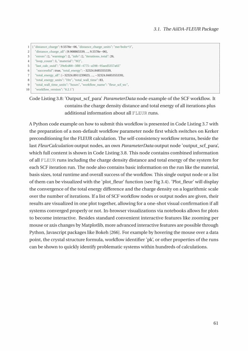
3.1. The AiiDA-FLEUR Package
1 { "distance_charge": 9.5578e−06, "distance_charge_units": "me/bohr^3",
2 "distance_charge_all": [9.908865339, ..., 9.5578e−06],
3 "errors": [], "warnings": [], "info": [], "iterations_total": 26,
4 "loop_count": 1, "material": "W2",
5 "last_calc_uuid": "29efcd00−3f8f−4775−a598−95aed5357a65"
6 "successful": true, "total_energy": −32324.8485355339,
7 "total_energy_all": [−32324.8911239023, ..., −32324.8485355339],
8 "total_energy_units": "Htr", "total_wall_time": 83,
9 "total_wall_time_units": "hours", "workflow_name": "fleur_scf_wc",
10 "workflow_version": "0.2.1"}
Code Listing 3.8: ’Output_scf_para’ ParameterData node example of the SCF workflow. It
contains the charge density distance and total energy of all iterations plus
additional information about all FLEUR runs.
A Python code example on how to submit this workflow is presented in Code Listing 3.7 with
the preparation of a non-default workflow parameter node first which switches on Kerker
preconditioning for the FLEUR calculation. The self-consistency workflow returns, beside the
last FleurCalculation output nodes, an own ParameterData output node ’output_scf_para’,
which full content is shown in Code Listing 3.8. This node contains combined information
of all FLEUR runs including the charge density distance and total energy of the system for
each SCF iteration run. The node also contains basic information on the run like the material,
basis sizes, total runtime and overall success of the workflow. This single output node or a list
of them can be visualized with the ’plot_fleur’ function (see Fig 3.4). ’Plot_fleur’ will display
the convergence of the total energy difference and the charge density on a logarithmic scale
over the number of iterations. If a list of SCF workflow nodes or output nodes are given, their
results are visualized in one plot together, allowing for a one-shot visual confirmation if all
systems converged properly or not. In-browser visualizations via notebooks allows for plots
to become interactive. Besides standard convenient interactive features like zooming per
mouse or axis changes by Matplotlib, more advanced interactive features are possible through
Python, Javascript packages like Bokeh [266]. For example by hovering the mouse over a data
point, the crystal structure formula, workflow identifier ’pk’, or other properties of the runs
can be shown to quickly identify problematic systems within hundreds of calculations.
61

3. Method Development
(a) Single SCF node visualization with
plot_fleur(<pk>).
(b) Multi SCF nodes visualization with
plot_fleur(list(<pks>)).
Fig. 3.4.: Default plot_fleur visualization for a single SCF workflow node (a) and multiple SCF
workflow nodes (b). Two logarithmic graphs are produced each, the convergence
of the charge density with respect to the iteration and the convergence behavior
of the total energy difference to the previous iteration with respect to the iteration
number. The multi node visualization is a collection of these SCF runs condensed in
one figure for each property.
62

3.1. The AiiDA-FLEUR Package
3.1.2.2. The DOS and Band Structure Workflows: fleur_DOS_w andfleur_band_wc
In order to calculate an electronic band structure and a density of states two workflows were
implemented. Since their workflow steps and database footprint (as shown in Fig 3.5) are
very similar, they are treated together in this subsection. These two workflows are mostly
deployed as a post-run on an already converged FleurCalculation. As input they therefore
need a RemoteData node from a previous calculation, a FleurinpData node and code nodes.
As optional input, similar to all other workflows, they take ’options’ and workflow control
parameter (’wf_parameters’) nodes. The content of their workflow parameter nodes as well
as a launch code example is shown in Code Listing 3.9. In the corresponding workflow
parameters one can adjust the number of k-points, smearing parameters and energy intervals.
In the control parameters for the band structure workflow a k-point path can be specified,
while for a good density of states calculation one wants to specify the k-point sampling
method. A quick plot_fleur visualization of a band structure and a density of states is shown
in Fig. 3.6. These graphs are meant only for quick examination. More advanced visualizations
for band structures, surface state highlighting, combined plots etc. are part of the ’masci-tools’
repository.
1 fleur_dos_wc = WorkflowFactory(’fleur.dos’)
2 fleur_band_wc = WorkflowFactory(’fleur.band’)
3 remote = load_node(<pk>)
4 fleurinp = load_node(<pk>)
5
6 wf_para_dos = ParameterData(dict={
7 ’tria’ : True, ’nkpts’ : 800, ’sigma’ : 0.005, ’emin’ : −0.30, ’emax’ : 0.80})
8 wf_para_band = ParameterData(dict={
9 ’kpath’ : ’auto’, ’nkpts’ : 800, ’sigma’ : 0.005, ’emin’ : −0.50, ’emax’ : 0.90})
10
11 # launch workflows
12 dos = submit(fleur_dos_wc, wf_parameters=wf_para_dos, fleurinp=fleurinp,
13 remote_data=remote, options=options, fleur=fleur, label="test dos",
14 description="fleur_dos test")
15 band = submit(fleur_band_wc, wf_parameters=wf_para_band, fleurinp=fleurinp,
16 remote_data=remote, options=options, fleur=fleur, label="test band",
17 description="fleur_band test")
Code Listing 3.9: Workflow control parameter specification example and launch code for a
density of states and a band structure workflow.
63
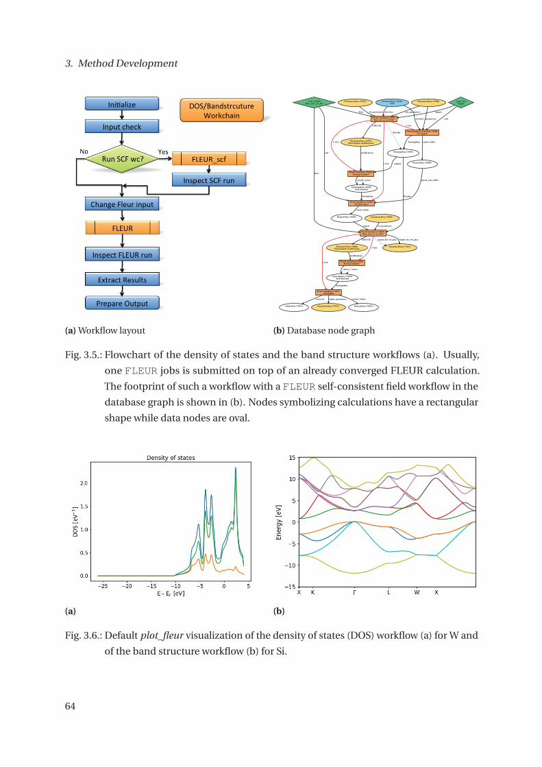
3. Method Development
(a) Workflow layout (b) Database node graph
Fig. 3.5.: Flowchart of the density of states and the band structure workflows (a). Usually,
one FLEUR jobs is submitted on top of an already converged FLEUR calculation.
The footprint of such a workflow with a FLEUR self-consistent field workflow in the
database graph is shown in (b). Nodes symbolizing calculations have a rectangular
shape while data nodes are oval.
(a) (b)
Fig. 3.6.: Default plot_fleur visualization of the density of states (DOS) workflow (a) for W and
of the band structure workflow (b) for Si.
64
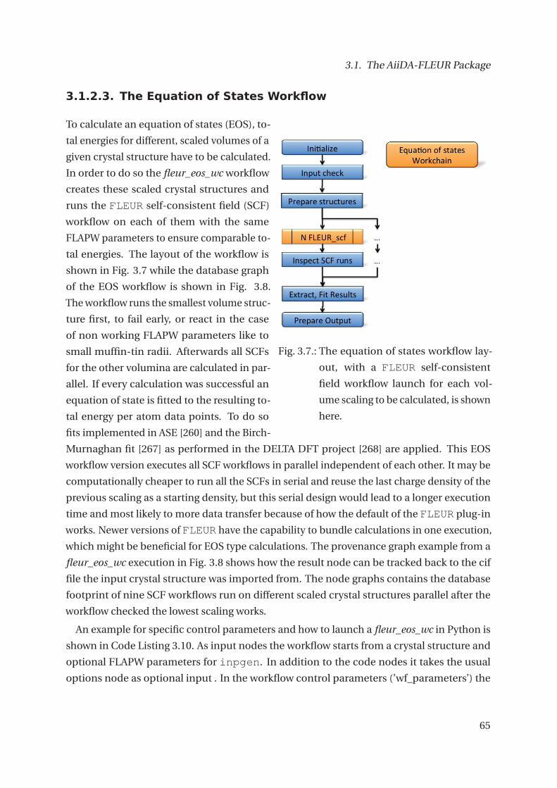
3.1. The AiiDA-FLEUR Package
3.1.2.3. The Equation of States Workflow
Fig. 3.7.: The equation of states workflow lay-
out, with a FLEUR self-consistent
field workflow launch for each vol-
ume scaling to be calculated, is shown
here.
To calculate an equation of states (EOS), to-
tal energies for different, scaled volumes of a
given crystal structure have to be calculated.
In order to do so the fleur_eos_wc workflow
creates these scaled crystal structures and
runs the FLEUR self-consistent field (SCF)
workflow on each of them with the same
FLAPW parameters to ensure comparable to-
tal energies. The layout of the workflow is
shown in Fig. 3.7 while the database graph
of the EOS workflow is shown in Fig. 3.8.
The workflow runs the smallest volume struc-
ture first, to fail early, or react in the case
of non working FLAPW parameters like to
small muffin-tin radii. Afterwards all SCFs
for the other volumina are calculated in par-
allel. If every calculation was successful an
equation of state is fitted to the resulting to-
tal energy per atom data points. To do so
fits implemented in ASE [260] and the Birch-
Murnaghan fit [267] as performed in the DELTA DFT project [268] are applied. This EOS
workflow version executes all SCF workflows in parallel independent of each other. It may be
computationally cheaper to run all the SCFs in serial and reuse the last charge density of the
previous scaling as a starting density, but this serial design would lead to a longer execution
time and most likely to more data transfer because of how the default of the FLEUR plug-in
works. Newer versions of FLEUR have the capability to bundle calculations in one execution,
which might be beneficial for EOS type calculations. The provenance graph example from a
fleur_eos_wc execution in Fig. 3.8 shows how the result node can be tracked back to the cif
file the input crystal structure was imported from. The node graphs contains the database
footprint of nine SCF workflows run on different scaled crystal structures parallel after the
workflow checked the lowest scaling works.
An example for specific control parameters and how to launch a fleur_eos_wc in Python is
shown in Code Listing 3.10. As input nodes the workflow starts from a crystal structure and
optional FLAPW parameters for inpgen. In addition to the code nodes it takes the usual
options node as optional input . In the workflow control parameters (’wf_parameters’) the
65

3. Method Development
Fig.3.8.:P
rovenan
cegrap
ho
fthe
equ
ation
ofstates
wo
rkflow
forFLEUR
inth
ed
atabase.In
this
examp
len
ine
scaling
po
ints
are
calculated
with
the
SCF
wo
rkflow
and
afterward
sa
com
bin
edo
utp
utn
od
ew
ithth
eeq
uatio
no
fstatesresu
ltsis
return
ed.
66
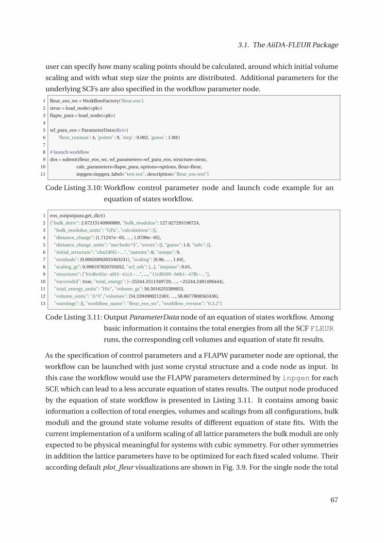
3.1. The AiiDA-FLEUR Package
user can specify how many scaling points should be calculated, around which initial volume
scaling and with what step size the points are distributed. Additional parameters for the
underlying SCFs are also specified in the workflow parameter node.
1 fleur_eos_wc = WorkflowFactory(’fleur.eos’)
2 struc = load_node(<pk>)
3 flapw_para = load_node(<pk>)
4
5 wf_para_eos = ParameterData(dict={
6 ’fleur_runmax’: 4, ’points’ : 9, ’step’ : 0.002, ’guess’ : 1.00})
7
8 # launch workflow
9 dos = submit(fleur_eos_wc, wf_parameters=wf_para_eos, structure=struc,
10 calc_parameters=flapw_para, options=options, fleur=fleur,
11 inpgen=inpgen, label="test eos", description="fleur_eos test")
Code Listing 3.10: Workflow control parameter node and launch code example for an
equation of states workflow.
1 eos_outputpara.get_dict()
2 {"bulk_deriv": 2.67215140960889, "bulk_modulus": 127.027293196724,
3 "bulk_modulus_units": "GPa", "calculations": [],
4 "distance_charge": [1.71247e−05, ... , 1.0709e−05],
5 "distance_charge_units": "me/bohr^3", "errors": [], "guess": 1.0, "info": [],
6 "initial_structure": "cba2df42−...", "natoms": 6, "nsteps": 9,
7 "residuals": [0.00020092833463241], "scaling": [0.96, ... , 1.04],
8 "scaling_gs": 0.998197820705052, "scf_wfs": [...], "stepsize": 0.01,
9 "structures": ["b1d6c05a−af43−41c2−...", ..., "11cf8599−b6b1−47fb−..."],
10 "successful": true, "total_energy": [−25244.2511349729, ..., −25244.2481496444],
11 "total_energy_units": "Htr", "volume_gs": 56.5016255389853,
12 "volume_units": "A^3","volumes": [54.3394900212401, ..., 58.8677808563436],
13 "warnings": [], "workflow_name": "fleur_eos_wc", "workflow_version": "0.3.2"}
Code Listing 3.11: Output ParameterData node of an equation of states workflow. Among
basic information it contains the total energies from all the SCF FLEUR
runs, the corresponding cell volumes and equation of state fit results.
As the specification of control parameters and a FLAPW parameter node are optional, the
workflow can be launched with just some crystal structure and a code node as input. In
this case the workflow would use the FLAPW parameters determined by inpgen for each
SCF, which can lead to a less accurate equation of states results. The output node produced
by the equation of state workflow is presented in Listing 3.11. It contains among basic
information a collection of total energies, volumes and scalings from all configurations, bulk
moduli and the ground state volume results of different equation of state fits. With the
current implementation of a uniform scaling of all lattice parameters the bulk moduli are only
expected to be physical meaningful for systems with cubic symmetry. For other symmetries
in addition the lattice parameters have to be optimized for each fixed scaled volume. Their
according default plot_fleur visualizations are shown in Fig. 3.9. For the single node the total
67

3. Method Development
(a) Single EOS node visualization (b) Multi EOS node visualization
Fig. 3.9.: Simple plot_fleur visualization of the equation of states workflow for a single node (a)
and a multi node visualization (b). In order to make the equation of state calculations
comparable, the total energies are plotted with respect to the total energy of the
lowest scaling.
energies for different relative volumes are visualized. In a multi node visualization several
equation of state results can be displayed together by plotting total energy differences with
respect to the system corespondent total energy of the lowest scaling data point.
3.1.3. Core-level Spectra Turn-key Solution
For the calculation of relevant spectral properties of X-ray photoelectron spectra from ab initio
as discussed in Section 2.9.2 two advanced workflows were implement. The initial_cls_wc
workflow for the calculation of initial-state core-level shifts (CLS) of metals and possibly
beyond. The second workflow with the potential to utilize a whole super compute cluster is
the core-hole workflow4. Its objective is to calculate core electron binding energies of a given
atomic configuration via core-hole simulations in a super cell setup. The layouts of these two
workflows are shown in Fig. 3.10.
In detail, the initial-state workflow calculates core-level shifts of a system with respect to
the elemental references via normal SCF calculations. If required, the SCF calculations of
4Some fictitious W-O example: The W-O alloy has 48 atoms in the unit cell with 4 tungsten atom-types by
symmetry and 8 oxygen symmetry types. A usual electronic configuration of tungsten has 17 core states
and for oxygen there are 2 core states. If one now wants to know the binding energies for all of these,
4 ·17+8 ·2+1 = 84 SCF supercell simulations can be deployed. A 2x2x2 super cell would have 384 atoms
which would be reasonable to run on 30 compute nodes each, totaling 2520 compute nodes for 84 jobs.
68

3.1. The AiiDA-FLEUR Package
(a) Initial-state workflow layout (b) Core-hole workflow layout
Fig. 3.10.: (a) Initial-state core-level shift workflow layout and (b) the layout of the core-hole
workflow. The initial-state workflow in (a) runs SCFs on the given crystal structure
and if needed on all elemental reference crystal structures needed for the calculation
of core-level shifts. the core-hole workflow in (b) runs one super cell simulation for a
structure without a core hole and compares its total energy to super cell calculations
with the core-hole setup of interest.
the corresponding elemental references are also managed by the workflow. Furthermore, the
workflow extracts the enthalpy of formation for the investigated compound from these SCF
runs. The workflow implements equation 2.42 for the calculation of core-level shifts as the
difference of Kohn-Sham core-level energies with respect to the Fermi energy. To minimize
uncertainties on CLS it is important that the compound as well as the reference systems are
calculated with the same atomic parameters (RMT, radial grid points and spacing, basis cutoff
�max). The workflow tests for this equality and tries to assure it, though it does not know
what is a good parameter set nor if the present set works well for both systems. Therefore,
it is currently best practice to enforce the FLAPW parameters used within the workflow, i.e.,
provide them as input for the system as for the references. A Python code example for the
69
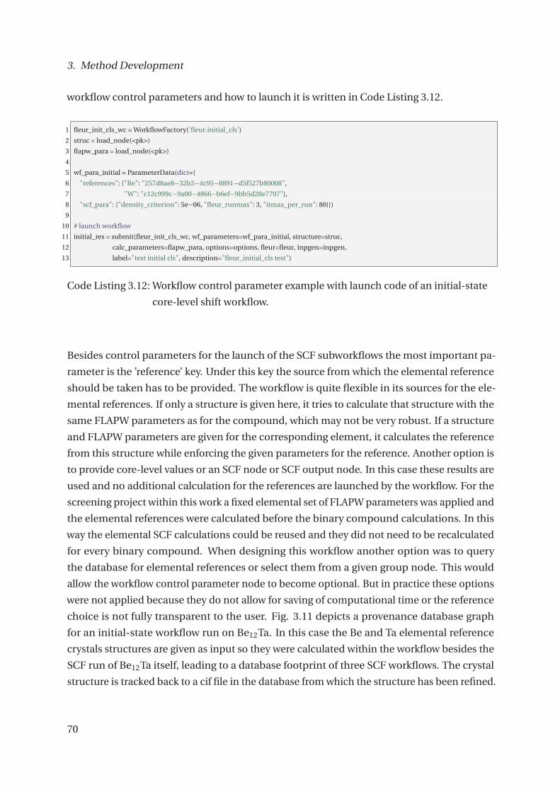
3. Method Development
workflow control parameters and how to launch it is written in Code Listing 3.12.
1 fleur_init_cls_wc = WorkflowFactory(’fleur.initial_cls’)
2 struc = load_node(<pk>)
3 flapw_para = load_node(<pk>)
4
5 wf_para_initial = ParameterData(dict={
6 "references": {"Be": "257d8ae8−32b3−4c95−8891−d5f527b80008",
7 "W": "c12c999c−9a00−4866−b6ef−9bb5d28e7797"},
8 "scf_para": {"density_criterion": 5e−06, "fleur_runmax": 3, "itmax_per_run": 80}})
9
10 # launch workflow
11 initial_res = submit(fleur_init_cls_wc, wf_parameters=wf_para_initial, structure=struc,
12 calc_parameters=flapw_para, options=options, fleur=fleur, inpgen=inpgen,
13 label="test initial cls", description="fleur_initial_cls test")
Code Listing 3.12: Workflow control parameter example with launch code of an initial-state
core-level shift workflow.
Besides control parameters for the launch of the SCF subworkflows the most important pa-
rameter is the ’reference’ key. Under this key the source from which the elemental reference
should be taken has to be provided. The workflow is quite flexible in its sources for the ele-
mental references. If only a structure is given here, it tries to calculate that structure with the
same FLAPW parameters as for the compound, which may not be very robust. If a structure
and FLAPW parameters are given for the corresponding element, it calculates the reference
from this structure while enforcing the given parameters for the reference. Another option is
to provide core-level values or an SCF node or SCF output node. In this case these results are
used and no additional calculation for the references are launched by the workflow. For the
screening project within this work a fixed elemental set of FLAPW parameters was applied and
the elemental references were calculated before the binary compound calculations. In this
way the elemental SCF calculations could be reused and they did not need to be recalculated
for every binary compound. When designing this workflow another option was to query
the database for elemental references or select them from a given group node. This would
allow the workflow control parameter node to become optional. But in practice these options
were not applied because they do not allow for saving of computational time or the reference
choice is not fully transparent to the user. Fig. 3.11 depicts a provenance database graph
for an initial-state workflow run on Be12Ta. In this case the Be and Ta elemental reference
crystals structures are given as input so they were calculated within the workflow besides the
SCF run of Be12Ta itself, leading to a database footprint of three SCF workflows. The crystal
structure is tracked back to a cif file in the database from which the structure has been refined.
70

3.1. The AiiDA-FLEUR Package
Wor
kCal
cula
tion
(658
26)
Para
met
erD
ata
(658
27)
outp
ut_i
nita
l_cl
s_w
c_pa
raou
tput
_ini
tal_
cls_
wc_
para
Wor
kCal
cula
tion
(419
80)
'fleu
r_in
itial
_cls
_wc
on B
e12T
a'
CA
LL
outp
ut_i
nita
l_cl
s_w
c_pa
ra
Wor
kCal
cula
tion
(563
50)
'cls
|scf
_wc
on r
ef T
a'
CA
LL
Wor
kCal
cula
tion
(419
87)
'cls
|scf
_wc
mai
n'
CA
LL
Para
met
erD
ata
(419
86)
CR
EA
TE
Wor
kCal
cula
tion
(563
49)
'cls
|scf
_wc
on r
ef B
e'
CA
LL
Para
met
erD
ata
(563
48)
CR
EA
TE
Para
met
erD
ata
(658
25)
CR
EA
TE
Fleu
rinp
utge
nCal
cula
tion
(586
69)
'scf
: inp
gen'
CA
LL
Fleu
rinp
Dat
a (5
9880
)
fleur
inp
Fleu
rCal
cula
tion
(602
60)
'scf
: fleu
r ru
n 1'
CA
LL
Para
met
erD
ata
(629
79)
last
_fleu
r_ca
lc_o
utpu
t
Wor
kCal
cula
tion
(657
98)
CA
LL
Para
met
erD
ata
(602
57)
'Fle
urin
pdat
a m
odifi
catio
ns'
CR
EA
TE
Wor
kCal
cula
tion
(602
58)
'fleu
rinp
mod
ifier
'CA
LL
Para
met
erD
ata
(657
97)
CR
EA
TE
Para
met
erD
ata
(657
99)
'out
put_
scf_
wc_
para
'
outp
ut_s
cf_w
c_pa
ra
Fleu
rinp
utge
nCal
cula
tion
(420
01)
'scf
: inp
gen'
CA
LL
Fleu
rinp
Dat
a (4
2015
)
fleur
inp
Wor
kCal
cula
tion
(420
23)
'fleu
rinp
mod
ifier
'
CA
LL
Fleu
rCal
cula
tion
(420
25)
'scf
: fleu
r ru
n 1'
CA
LL
Para
met
erD
ata
(547
98)
last
_fleu
r_ca
lc_o
utpu
t
Para
met
erD
ata
(420
22)
'Fle
urin
pdat
a m
odifi
catio
ns'
CR
EA
TE
Para
met
erD
ata
(558
73)
CR
EA
TE
Wor
kCal
cula
tion
(558
74)
CA
LL
Para
met
erD
ata
(558
75)
'out
put_
scf_
wc_
para
'
outp
ut_s
cf_w
c_pa
ra
wf_
para
met
ers
Fleu
rinp
utge
nCal
cula
tion
(581
03)
'scf
: inp
gen'
CA
LL
Fleu
rinp
Dat
a (5
9683
)
fleur
inp
Wor
kCal
cula
tion
(597
73)
'fleu
rinp
mod
ifier
'
CA
LL
Fleu
rCal
cula
tion
(597
77)
'scf
: fleu
r ru
n 1'
CA
LL
Para
met
erD
ata
(629
51)
last
_fleu
r_ca
lc_o
utpu
t
Wor
kCal
cula
tion
(657
95)
CA
LL
Para
met
erD
ata
(597
71)
'Fle
urin
pdat
a m
odifi
catio
ns'
CR
EA
TE
Para
met
erD
ata
(657
94)
CR
EA
TE
Para
met
erD
ata
(657
96)
'out
put_
scf_
wc_
para
'
outp
ut_s
cf_w
c_pa
ra
wf_
para
met
ers
wf_
para
met
ers
resu
lts_n
ode
Stru
ctur
eDat
a (2
4006
) B
e
stru
ctur
e
stru
ctur
e
Rem
oteD
ata
(588
95)
rem
ote_
fold
er
fleur
inpD
ata
pare
nt_c
alc_
fold
er
orig
inal
Para
met
erD
ata
(385
03)
calc
_par
amet
ers
para
met
ers
Rem
oteD
ata
(589
72)
rem
ote_
fold
erfle
urin
pDat
a
pare
nt_c
alc_
fold
er
orig
inal
outp
ut_p
aram
eter
s
Stru
ctur
eDat
a (1
26)
Ta
Wor
kCal
cula
tion
(384
87)
stru
ctur
e
Stru
ctur
eDat
a (3
8488
)' p
rim
itive
'
_ret
urn
_ret
urn
stru
ctur
e
stru
ctur
e
Fleu
rinp
Dat
a (5
9774
)'m
od_fl
euri
np'
_ret
urn
_ret
urn
fleur
inpd
ata
outp
ut_p
aram
eter
s
last
_cal
c_ou
t
outp
ut_s
cf_w
c_pa
raou
tput
_scf
_wc_
para
fleur
inpD
ata
Rem
oteD
ata
(420
06)
rem
ote_
fold
er
orig
inal
pare
nt_c
alc_
fold
er
Fleu
rinp
Dat
a (4
2024
)'m
od_fl
euri
np'
_ret
urn
_ret
urn
last
_cal
c_ou
t
outp
ut_s
cf_w
c_pa
raou
tput
_scf
_wc_
para
mod
ifica
tions
Fleu
rinp
Dat
a (6
0259
)'m
od_fl
euri
np'
_ret
urn
_ret
urn
outp
ara
calc
_ref
1
outp
ut_p
aram
eter
s
last
_cal
c_ou
t
mod
ifica
tions
outp
ara
outp
ut_s
cf_w
c_pa
raou
tput
_scf
_wc_
para
inpu
t_st
ruct
ure
Cod
e (1
51)
'inpg
en'
inpg
en
inpg
enin
pgen
inpg
en
code
code
code
Para
met
erD
ata
(419
79)
wf_
para
met
ers
Para
met
erD
ata
(419
73)
calc
_par
amet
ers
calc
_par
amet
ers
para
met
ers
Stru
ctur
eDat
a (3
8426
)' p
rim
itive
'
stru
ctur
e
stru
ctur
e
stru
ctur
e
Cod
e (6
)'fl
eur_
mpi
_v0.
28'
fleur
fleur
fleur
fleur
code
code
code
fleur
inpd
ata
mod
ifica
tions
outp
ara
calc
_ref
0
Stru
ctur
eDat
a (1
40)
Be
Wor
kCal
cula
tion
(240
05)
stru
ctur
e
_ret
urn
_ret
urn
Para
met
erD
ata
(419
68)
calc
_par
amet
ers
para
met
ers
fleur
inpd
ata
Cif
Dat
a (3
7074
)
Wor
kCal
cula
tion
(370
83)
cif
Stru
ctur
eDat
a (3
7084
) B
e12T
a
_ret
urn_
retu
rn
Wor
kCal
cula
tion
(384
25)
stru
ctur
e
_ret
urn_
retu
rn
Fig
.3.1
1.:P
rove
nan
cegr
aph
ofth
ein
itia
l-st
ate
core
-lev
elsh
iftw
orkfl
owon
Be 1
2Ta
inth
ed
atab
ase
wit
hd
ata
and
logi
clin
ks.I
nth
is
case
the
stru
ctu
reis
trac
ked
bac
kto
aci
ffile
and
the
Be
and
Tare
fere
nce
sar
eca
lcu
late
dex
plic
itly
,lea
din
gto
ad
atab
ase
foo
tpri
nto
fth
ree
SCF
wo
rkfl
ows.
71
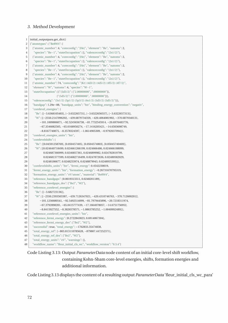
3. Method Development
1 initial_outputpara.get_dict()
2 {"atomtypes": {"Be8W4": [
3 {"atomic_number": 4, "coreconfig": "[He]", "element": "Be", "natoms": 2,
4 "species": "Be−1", "stateOccupation": [], "valenceconfig": "(2s1/2)"},
5 {"atomic_number": 4, "coreconfig": "[He]", "element": "Be", "natoms": 2,
6 "species": "Be−1", "stateOccupation": [], "valenceconfig": "(2s1/2)"},
7 {"atomic_number": 4, "coreconfig": "[He]", "element": "Be", "natoms": 2,
8 "species": "Be−1", "stateOccupation": [], "valenceconfig": "(2s1/2)"},
9 {"atomic_number": 4, "coreconfig": "[He]", "element": "Be", "natoms": 2,
10 "species": "Be−1", "stateOccupation": [], "valenceconfig": "(2s1/2)"},
11 {"atomic_number": 74, "coreconfig": "[Kr] (4d3/2) (4d5/2) (4f5/2) (4f7/2)",
12 "element": "W", "natoms": 4, "species": "W−1",
13 "stateOccupation": [{"(5d3/2)": ["2.00000000", ".00000000"]},
14 {"(5d5/2)": ["2.00000000", ".00000000"]}],
15 "valenceconfig": "(5s1/2) (5p1/2) (5p3/2) (6s1/2) (5d3/2) (5d5/2)"}]},
16 "bandgap": 1.29e−08, "bandgap_units": "htr", "binding_energy_convention": "negativ",
17 "corelevel_energies": {
18 "Be": [[−3.6368105483], [−3.632265731], [−3.6322656557], [−3.6322657313]],
19 "W": [[−2550.2147096202, −439.6879734359, −420.4064081902, −370.6879340131,
20 −101.1009806871, −92.5245656738, −81.7732545914, −20.6970483776,
21 −67.3546082505, −65.0168950274, −17.1416205421, −14.6503698749,
22 −8.8167740875, −8.3578324597, −1.0614905309, −0.9792037094]]},
23 "corelevel_energies_units": "htr",
24 "corelevelshifts": {
25 "Be": [[0.04591258769], [0.050457405], [0.0504574803], [0.05045740469]],
26 "W": [[0.024640718499, 0.024661266199, 0.024666486, 0.024666188099,
27 0.024687366999, 0.0246857361, 0.0246899982, 0.024782819799,
28 0.024681577599, 0.024682716499, 0.0247872636, 0.02480582029,
29 0.0248186677, 0.0248253974, 0.0248879943, 0.0248955395]]},
30 "corelevelshifts_units": "htr", "fermi_energy": 0.4542230019,
31 "fermi_energy_units": "htr", "formation_energy": −0.26731670795319,
32 "formation_energy_units": "eV/atom", "material": "Be8W4",
33 "reference_bandgaps": [0.0019313311, 0.0248201189],
34 "reference_bandgaps_des": ["Be2", "W2"],
35 "reference_corelevel_energies": {
36 "Be": [[−3.682723136]],
37 "W": [[−2550.2393503387, −439.7126347021, −420.4310746763, −370.7126002012,
38 −101.1256680541, −92.5492514099, −81.7979445896, −20.7218311974,
39 −67.3792898281, −65.0415777439, −17.1664078057, −14.6751756952,
40 −8.8415927552, −8.3826578571, −1.0863785252, −1.0040992489]]},
41 "reference_corelevel_energies_units": "htr",
42 "reference_fermi_energy": [0.2722843823, 0.6914067304],
43 "reference_fermi_energy_des": ["Be2", "W2"],
44 "successful": true, "total_energy": −1762833.35474838,
45 "total_energy_ref": [−803.813110785628, −879807.447252371],
46 "total_energy_ref_des": ["Be2", "W2"],
47 "total_energy_units": "eV", "warnings": [],
48 "workflow_name": "fleur_initial_cls_wc", "workflow_version": "0.3.4"}
Code Listing 3.13: Output ParameterData node content of an initial core-level shift workflow,
containing Kohn-Sham core-level energies, shifts, formation energies and
additional information.
Code Listing 3.13 displays the content of a resulting output ParameterData ’fleur_initial_cls_wc_para’
72

3.1. The AiiDA-FLEUR Package
node. The node contains detailed information about the atom-types and their electronic
configuration in a nested dictionary list structure for the calculated compound. Additionally,
the node contains core-level energies, some basic run information , core-level shifts, total
energy, band gap and Fermi energy for the compound and the reference systems. Overall, this
node contains all information to construct a relative core-level spectrum or evaluate all shifts
for any other reference.
The core-hole workflow can be deployed to calculate absolute core-level binding energies.
From a computational cost perspective it may be cheaper to calculate all relative initial-state
shifts of a structure and then launch one core-hole calculation on the structure to get an
absolute reference energy instead of performing expensive core-hole calculations for all
atom-types in the structure. The core-hole workflow implements the usual FLEUR workflow
interface with a workflow control parameter node. The contents of this node and a Python
launch code example are shown in Code Listing 3.14.
1 fleur_corehole_wc = WorkflowFactory(’fleur.corehole’)
2
3 struc = load_node(<pk>)
4 flapw_para = load_node(<pk>)
5
6 wf_para_corehole = ParameterData(dict={u’atoms’: [u’Be’], #[u’all’],
7 u’supercell_size’: [2, 2, 2], u’corelevel’: [’1s’], #[u’all’],
8 u’hole_charge’: 1.0, u’magnetic’: True, u’method’: u’valence’, u’serial’: False}
9
10 # launch workflow
11 dos = submit(fleur_corehole_wc, wf_parameters=wf_para_corehole, structure=struc,
12 calc_parameters=flapw_para, options=options,
13 fleur=fleur, inpgen=inpgen, label="test core hole wc",
14 description="fleur_corehole test")
Code Listing 3.14: Control parameter and launch code example for a core-hole workflow to
calculate a full 1s valence core hole for all Be atomtypes in some Beryllide
with a 2x2x2 supercell.
The control parameters contain keys to specify the type of core-hole calculations performed
on which atoms and which core levels. With the ’atoms’ key a list of atoms is specified
on which to place a core hole. They can be specified as strings, as positions, or number
in the atom list of the AiiDA StructureData. If core-hole calculations on all atomtypes of
one element should be deployed, one can specify the element as a string. If the binding
energies for all elements and atom-types should be calculated, ’all’ can be specified. With
the ’corelevel’ key the user specifies for which core levels a core-hole calculation should
be launched. Possible specifications are ’all’, core states like 1s, 2p1/2, etc or an element
specification as prefix i.e., ’Be1s’. Furthermore, the core-hole charge (’hole_charge’) and
the type of the core hole can be specified. The type of the ’method’ key can be ’valence’
73

3. Method Development
resulting in the core electron to be put into the valence band or ’charge’ which results in
a simple removal of the electron leaving a charged system. Core-hole calculations often
require the introduction of magnetism into the system, making it important to perform spin
polarized calculation, which might be switched off with the ’magnetic’ key. The workflow
only launches a series of single core-hole calculations though it can be easily extended to the
use case of multiple core holes within one structure. Since the electronic configuration is
currently not always written to the ’inp.xml’ by FLEUR or inpgen, it is important to either
enforce an electronic configuration if FLAPW parameters are provided, or to make sure that
the electronic configuration is written explicitly in the ’inp.xml’ if a FleurinpData node is
provided. Otherwise the workflow might struggle preparing the input correctly or FLEUR
calculations might fail. The super cell size to be calculated is specified with the ’supercell_size’
key as a list of integers in the workflow control parameters. During a workflow run the crystal
cells will be adjusted such that the atom with the core hole lies at the coordinate system’s
origin to avoid non-symmorphic symmetries. Since we want to compare the total energy of
super cell calculations with and without core hole, the workflow first calls the SCF-workflow
to convergence a super cell system without core hole. This has two advantages. First, if this
SCF already fails, the other expensive calculations are not launched. Second, all the core-
hole calculations can start from the converged charge density of the super cell calculation
without core hole to save computational time and to make the calculation more stable, at
least for small core-hole charges. Then, all core-hole calculations are launched in parallel
by the workflow. The database footprint of a deployed core-hole workflow on a simple Si
system to calculate 2p binding energies for two atom-types is shown in Fig. 3.12. In total
five SCF workflows are run, one for the reference super cell and four core-hole calculations.
74

3.1. The AiiDA-FLEUR Package
1 corehole_outputpara.get_dict()
2 {"atomtypes": [[
3 {"atomic_number": 4, "coreconfig": "(1s1/2)", "element": "Be", "natoms": 1,
4 "species": "Be_corehole1", "stateOccupation": [
5 {"(1s1/2)": ["1.00000000", ".50000000"]},
6 {"(2p1/2)": [".50000000", ".00000000"]}], "valenceconfig": "(2s1/2) (2p1/2)"},
7 {"atomic_number": 4, "coreconfig": "[He]", "element": "Be", "natoms": 1,
8 "species": "Be−2", "stateOccupation": [{"(2p1/2)": [".00000000", ".00000000"]}],
9 "valenceconfig": "(2s1/2) (2p1/2)"},
10 {"atomic_number": 4, "coreconfig": "[He]", "element": "Be", "natoms": 1,
11 "species": "Be−2", "stateOccupation": [{"(2p1/2)": [".00000000", ".00000000"]}],
12 "valenceconfig": "(2s1/2) (2p1/2)"},
13 {"atomic_number": 4, "coreconfig": "[He]", "element": "Be", "natoms": 1,
14 "species": "Be−2", "stateOccupation": [{"(2p1/2)": [".00000000", ".00000000"]}],
15 "valenceconfig": "(2s1/2) (2p1/2)"}]], "bandgap": [0.0004425914],
16 "bandgap_units":"eV", "binding_energy": [53.57027767044], "corehole_type": "valence",
17 "binding_energy_units": "eV", "binding_energy_convention": "negativ",
18 "coreholes_calculated": "Be1s", "coreholes_calculated_details": "", "coresetup": [],
19 "errors": [], "fermi_energy": [0.3138075709], "fermi_energy_unit": "eV",
20 "reference_bandgaps": [0.0225936434], "reference_coresetup": [],
21 "successful": true, "total_energy_all": [−1554.08485250996],
22 "total_energy_all_units": "eV", "total_energy_ref": [−1607.6551301804],
23 "total_energy_ref_units": "eV", "warnings": [], "hints": [],
24 "weighted_binding_energy": [107.14055534088], "weighted_binding_energy_units": "eV",
25 "workflow_name": "fleur_corehole_wc", "workflow_version": "0.3.2"}
Code Listing 3.15: Output ParameterData node of a simple core-hole workflow run to
calculate a spin-polarized half-valence core hole of elemental Be.
The main output result node for a core-hole workflow run on a simple pure Be system is
shown in Listing 3.15. On an elemental Be structure a half-valence core-hole calculation was
performed with a 2x2x2 super cell. The output node contains total energies of the core-hole
system and the reference system as well as core-level binding energies and the weighted
binding energies with charge one. Additional information on the atom-types of each run with
details of the core-hole setup are in the output node together with the Fermi energies and
bandgaps.
75

3. Method Development
Fig.3.12.:C
ore-h
ole
wo
rkflow
datab
asep
rovenan
cegrap
h.
Th
isgrap
hd
isplays
the
no
des
pro
du
cedb
ya
run
of
the
core-h
ole
wo
rkflow
tocalcu
late2p
bin
din
gen
ergieso
faSisin
glecrystal.Fo
ur
SCF
wo
rkflow
sare
run
on
sup
ercellsetu
ps.
76
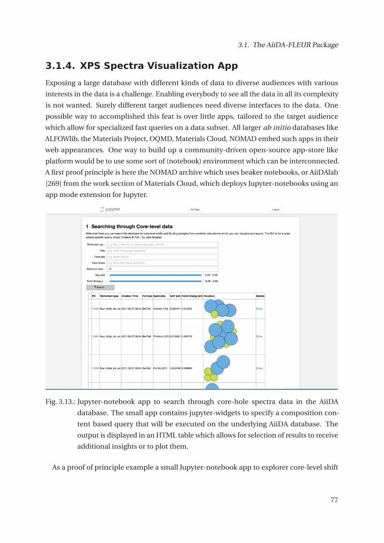
3.1. The AiiDA-FLEUR Package
3.1.4. XPS Spectra Visualization App
Exposing a large database with different kinds of data to diverse audiences with various
interests in the data is a challenge. Enabling everybody to see all the data in all its complexity
is not wanted. Surely different target audiences need diverse interfaces to the data. One
possible way to accomplished this feat is over little apps, tailored to the target audience
which allow for specialized fast queries on a data subset. All larger ab initio databases like
ALFOWlib, the Materials Project, OQMD, Materials Cloud, NOMAD embed such apps in their
web appearances. One way to build up a community-driven open-source app-store like
platform would be to use some sort of (notebook) environment which can be interconnected.
A first proof principle is here the NOMAD archive which uses beaker notebooks, or AiiDAlab
[269] from the work section of Materials Cloud, which deploys Jupyter-notebooks using an
app mode extension for Jupyter.
Fig. 3.13.: Jupyter-notebook app to search through core-hole spectra data in the AiiDA
database. The small app contains jupyter-widgets to specify a composition con-
tent based query that will be executed on the underlying AiiDA database. The
output is displayed in an HTML table which allows for selection of results to receive
additional insights or to plot them.
As a proof of principle example a small Jupyter-notebook app to explorer core-level shift
77

3. Method Development
(a)
(b)
Fig. 3.14.: Jupyter-notebook app to visualize core-hole spectra data. From the results of differ-
ent systems any composition of mixed spectra can be constructed with different
peak functions, resolution and broadenings. The app displays the constructed
spectra as well as the ab initio data set from which it was generated and allows for
extraction of these data and theoretical spectra.78

3.2. Fitting XPS Spectra from a Complete ab initio Dataset
data was developed and is shown in Fig. 3.13. The first notebook interfaces a small special
query of the underlying database for successful core-level workflows and displaying the query
results in an HTML table. With Jupyter widgets the user can refine the query. For example
the user can decide what elements or formulas he wants to find results for. Furthermore, the
workflow type, number of returned results, band gap, Fermi energy and core levels can be
specified to refine the query. Through clicking a button the query is executed and the results
rendered within an HTML table with some basic information from the database and a preview
of the crystal structures. From this table the user can display in detail results about certain
runs or select as many results as wanted and construct a theoretical spectrum for them. The
spectrum visualization is provided by the functionality of a second notebook shown in Fig.
3.14. This Jupyter-notebook app plots the core-level shifts results from selected database
entries. Furthermore, the app displays the raw data and constructs a simple theoretical
spectrum from these core-level shifts by the broadening of the shifts through peak functions.
Through Jupyter widgets the notebook allows the user to weight results of database entries
and to specify the energy range of the plots, the peak function type and parameters of the
peak functions like the gaussian or lorentzian broadenings. The data for the constructed
spectrum can be downloaded, exported via a download button.
3.2. Fitting XPS Spectra from a Complete ab
initio Dataset
In the theory sections (2.9.1 and 2.9.2) it was laid-out what challenges lie in the chemical
interpretation of X-ray photoelectron spectra and which spectral properties can be calculated
from ab initio methods, in particular with the FLEUR code. In section 3.1.3 the turn-key solu-
tion workflows were explained which enable among such spectral properties the calculation
of core-level shifts and binding energies.
While comparing simulations results to experimental data we realized that theoretical
information on the chemical shifts and the binding energies alone is often not comparable
to traditional fit results in the case of most XPS spectra of beryllides. Thus having only
theoretical chemical shift data helped little with the chemical interpretation of the spectra.
The following reasons for this were identified. One compound can have several different
chemical environments of the same element due to the symmetries of the crystal. For example
in the case of Be12Ti (I 4/mmm) there are three different Be atom symmetry types with four
Be atoms each in a unit cell. These Be atom-types turn out to have each a different core-level
shift. Having spectral contributions from several symmetry types per element is not new and
long known in the chemistry community for molecules or surface core-level shifts. Though
79

3. Method Development
for solids there is mostly one reported shift per compound and element in the numerical
XPS databases like NIST [90]. While for molecules the individual chemical environments
can be very distinct in their response, for solid state spectra of metals the chemical shifts
are often to close together to be fitted separately within the resolution of the experiment.
Mathematically the sum of two peak profiles at different means and areas is not a peak profile
function again. In general, the sum lies outside of the profile function set and one cannot
expect parameters resulting from experimental fits and to some extend reported literature
values to be comparable to theoretical predictions of core-level shifts and binding energies
for materials with several diverse chemical environments of the same element (at least within
the accuracy needed).
Fig. 3.15.: Number of atom-types by symmetry (non-equivalent atoms) of ~31000 binary struc-
tures from the ICSD in an logarithmic histogram. The atom-types are determined
with spglib using ’equivalent_atoms’. 52 % of the structures have more than one
atom-type per element. A larger number of atom-types increases the complexity
and problems of the traditional XPS fitting procedures.
Of the ~31000 structures of the non-unique binary compounds in the ICSD around 52
% have at least one element in several symmetry positions and possible different chemical
environments (see Fig. 3.15). This fraction will likely increase for larger and complexer
structural configurations like ternary compounds and beyond. The number of atom-types
80

3.2. Fitting XPS Spectra from a Complete ab initio Dataset
was determined with spglib [178]. While for 48 % of the binaries there is no problem with
the traditional fitting approach, for the rest it should be applied more carefully, which is
marked by the black line in the histogram. For more precise information on where problems
are expected the structures have to be filtered for uniqueness, trash structures have to be
sorted out through ab initio calculations and the chemical shifts for the atom-types have to
be calculated.
Since the fit parameters are often neither comparable to theoretical predictions nor to
literature values of individual phase components it can be argued that the interpretation
of the traditional experimental fitting approach with nearly no constraints and no a priori
knowledge of mixed systems cannot lead to a successful chemical interpretation of phase
content for complex spectra. The traditional evaluation approach works well for materials
with one effective chemical environment per element and where the chemical shift of a
compound is well separated from other chemical shifts in the phase diagram. If the full form
of all individual pure phase spectra is experimentally known, the fit parameters can be reused
for the evaluation of the phase content [78]. Such a procedure is slow, cost intensive and
applied in some specific (industrial) applications where a lot of similar spectra are evaluated.
As a way out of this problem theoretical spectra are constructed within this work and then
fitted directly to experimental data with more constraints and a priori knowledge. In order to
construct such a theoretical X-ray photoelectron spectrum from chemical shifts and binding
energies which can be curve fitted to experimental data directly, two kinds of information
are required. First, the absolute binding energies of all chemical environments from all
phases that might contribute to the spectrum and second an intensity contribution factor
for each chemical environment of these phases to the spectrum. Ab initio simulations can
provide the binding energies and/or chemical shifts. The chemical shifts are converted into
absolute binding energies with respect to an elemental experimental, or theoretical, binding
energy reference EB, ref of the core state of interest. The intensity contribution is estimated
with the knowledge of the crystal structure via the number of atoms of the same element
per non-equivalent atom-type multiplied with the number of electrons from the core level
contributing to the spectrum.
A theoretical ab initio spectrum fit function Stheo(E) is constructed in detail as follows,
Sexp(E) = Stheo(E)+Bexp(E) (3.1)
Stheo(E) =N∑
i=1λiΦcomp, i(E) (3.2)
Φcomp, i(E) =M∑
j=1α j Vj (E ,μj, fG, fL) (3.3)
81

3. Method Development
Vj (E ,μj, fG, fL) =Re
[ω
(�ln(2)(2(E−μj)−i fL)
fG
)]
fG
�π
2�
ln(2)
(3.4)
μj,�m = EB, ref −Cj,�m (3.5)
where Bexp(E) is the spectrum’s background from the experiment, which has to be added
to the theoretically constructed spectrum Stheo(E) for fitting (Eq. 3.1). Stheo(E) is a linear
combination of N phases with a concentration fit parameter λi for each phase and its corre-
sponding phase spectrum Φcomp, i(E ) (Eq. 3.2). The phase spectra (Eq. 3.3) are constructed by
weighting normed peak-functions Vj with an intensity factor α j for each of the M chemical
environments. In this work αj is the total number of electrons of a core level contributing
from all atoms from atom-type j (i.e., for a W 4f 7/2 core-state αj would be 8 times the num-
ber of W atoms of type j). This assumption on the intensity information extracted from the
contributing atom-types for solids is only valid if differences in the cross sections, angular
dependence, other scattering properties, electron transport properties and the spatial photon
density for the same orbitals on all atom-types throughout a unit cell are negligible. This
might not be the case anymore for very large unit cells, since XPS is very surface sensitive.
Effects like shake ups, satellites, Costa-Kronig may change relative intensity factors of certain
core levels.
As peak function Voigt profiles Vj are deployed, while for transition metals the asymmetric
LA line shape is applied (see equation 2.38 from section 2.9.1). A very accurate explicit (without
convolution integral) representation of a Voigt profiles is possible through the Faddeeva
function (ω), as shown by Eq. 3.4, where fG, fL are the Gaussian and Lorentzian full width
half maxima and the profile mean is μj. The Faddeeva function is included in scientific
Python packages. The full width half maxima, fG, fL, are also optimized in the fitting and are
assumed within this work to be the same for all Vj for a certain core-level and for all phases i.
The mean μj is the binding energy of the chemical environment j. Ab initio chemical shifts
Cj,�m are converted into absolute binding energies with respect to an elemental, binding
energy value EB, ref of the core state of interest (Eq. 3.5). These theoretical or experimental
elemental reference binding energies have uncertainties from ~0.06 eV up to 0.6 eV in the
NIST XPS database [90]. Therefore, the reference energy may need to be optimized within
its uncertainty. This optimization is also helpful to compensate differences in the energy
scale calibration from the experiment to the reference measurement. Furthermore, fitting the
reference binding energy allows for compensation of systematic errors of the ab initio data. In
the fits shown in Section 4.3 only one reference energy per mixed phase core-level spectrum
is fitted.
When fitting splitted core states only one peak is constructed with all degrees of freedom
82
3.2. Fitting XPS Spectra from a Complete ab initio Dataset
the other(s) are fitted with the same parameters and constant offset for the splitting. Phase
concentrations of best fits for individual high-resolution spectra of the same sample are not
enforced to yield the same results. Several core-level spectra from the same sample can be
fitted at once for example the Be 1s and W 4f region of a Be-W alloy. This way the fit is enforced
to use the same phase concentration ratios, reducing the degrees of freedom in the fit.
The spectra interpretation with this physically motivated fit can be automated, by beginning
to fit all possible phases with the corresponding elements and sort out phases that do not
contribute to the spectrum, then reiterate. Contribution is determined by the concentration
values and their uncertainty. Chemical shifts of different phases may not be unique. If the in-
tensity factors and chemical shifts are the same, the phase spectra become indistinguishable.
This fit method in principle enables to find all these non-unique spectrum interpretations, i.e.
linear dependencies. The fitting procedure needs less fit parameters than the current conven-
tional way of fitting an X-ray photoelectron spectrum, making it beneficial and scalable for
the interpretation of more complex spectra, with many different chemical environments. For
very simple XPS spectra with phases with only one contribution, the number of fit parameters
is the same as for the conventional way.
Notice, that still a complete chemical shift database and intensity estimation for the system
of interest is necessary for a trustworthy interpretation. However, one advantage is that
constraints from experimental knowledge (i.e., measured stoichiometry) can be incorporated
into the fit. The proposed spectra construction does not contain any additional physics
and features that might occur in XPS spectra as introduced in section 2.9 and described in
[218] like satellites, plasmons, shake-up, shake-off, Auger peaks. Also currently a consistent
background estimation is also not included in the fit. Overall, the fitting procedure may be
advanced in ways to comprehend these needs too. For the fitted well-behaved beryllides
spectra examined in detail within this work these issues are not relevant.
In retrospect the method has some similarities to the evaluation of XAS spectra reported in
the work of K. Mathew et al. [140] in nature scientific data. The method has also advantages
over pure experimental approaches which measure all single phase spectra to determine
signal ratios like in [78]. This component-fit method is not the same as a Principal Component
Analysis (PCA) [270], because our components are physical motivated, known and not altered
or orthogonalized to constructed principal components. If our fit succeeds there is a direct
chemical interpretation connected to it. Being pure mathematical a PCA usually goes the
other way, to find similarities in a series of XPS spectra [271, 272] (functions), the resulting
mathematical orthogonal principle components do not need to have any physical meaning
and may not lead to a precise chemical interpretation [273] at all. The resulting principle
components can even be partly negative and therefore unphysical. Our evaluation procedure
83

3. Method Development
and proof of concept led to a pending international patent application and is on the way to
be published in a separate publication.
3.3. Method Development Sum-up
In order to enable provenance tracked ab initio all-electron high-throughput simulations
the FLEUR code was connected to the AiiDA framework. This was accomplished through
the implementation of AiiDA plug-ins and workflows. Workflows are powerful simulation
protocols, containing expert knowledge. The FLEUR plug-ins, workflows and tools form to-
gether the AiiDA-FLEUR python package, which is open source under MIT license. Workflows
and tools account for a high-level work environment, increase productivity by decreasing
the required time to solution drastically. Basic workflows for everyday simulations with the
FLEUR code were implemented. These workflows form the backbone of more advanced
workflows like the implemented workflows to calculate core-level properties for X-ray photo-
electron spectroscopy. Since these theoretical core-level properties were hard to compare for
complexer chemical environments directly to traditional fit results of experimental spectra,
we developed and implemented a first proof of principle tool to fit XPS spectra directly from
ab initio data alone. This resulted in a pending international patent application and a small
app to search and access the simulations results from a database for fitting spectra. The
workflows, fitting procedure and the database access app lay out a first version for a scalable
turn-key solution for XPS spectra. The spectral fitting has to be advanced in various ways
for systems outside of the scope of this work and is not blindly applicable. For example the
spectral background is not yet consistently determined within the fit itself. Also special peak
area ratios, satellites peaks, shake-up, shake-off, and plasmon excitation contributions have
to be removed currently from the spectra before hand, or accounted for somehow.
84
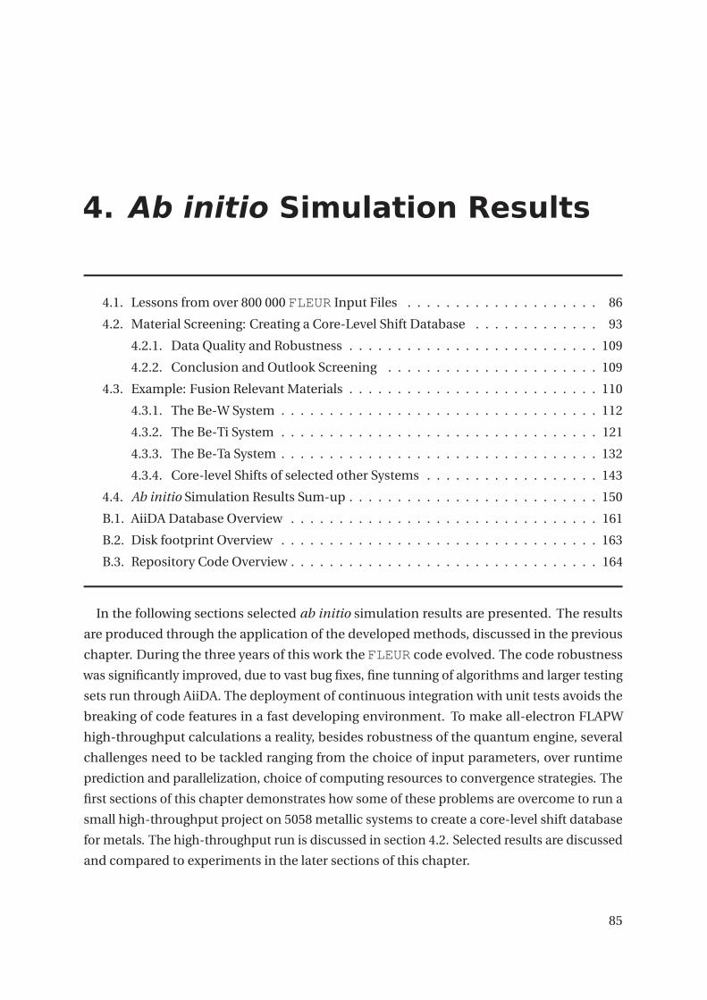
4. Ab initio Simulation Results
4.1. Lessons from over 800 000 FLEUR Input Files . . . . . . . . . . . . . . . . . . . . 86
4.2. Material Screening: Creating a Core-Level Shift Database . . . . . . . . . . . . . 93
4.2.1. Data Quality and Robustness . . . . . . . . . . . . . . . . . . . . . . . . . . 109
4.2.2. Conclusion and Outlook Screening . . . . . . . . . . . . . . . . . . . . . . 109
4.3. Example: Fusion Relevant Materials . . . . . . . . . . . . . . . . . . . . . . . . . . 110
4.3.1. The Be-W System . . . . . . . . . . . . . . . . . . . . . . . . . . . . . . . . . 112
4.3.2. The Be-Ti System . . . . . . . . . . . . . . . . . . . . . . . . . . . . . . . . . 121
4.3.3. The Be-Ta System . . . . . . . . . . . . . . . . . . . . . . . . . . . . . . . . . 132
4.3.4. Core-level Shifts of selected other Systems . . . . . . . . . . . . . . . . . . 143
4.4. Ab initio Simulation Results Sum-up . . . . . . . . . . . . . . . . . . . . . . . . . . 150
B.1. AiiDA Database Overview . . . . . . . . . . . . . . . . . . . . . . . . . . . . . . . . 161
B.2. Disk footprint Overview . . . . . . . . . . . . . . . . . . . . . . . . . . . . . . . . . 163
B.3. Repository Code Overview . . . . . . . . . . . . . . . . . . . . . . . . . . . . . . . . 164
In the following sections selected ab initio simulation results are presented. The results
are produced through the application of the developed methods, discussed in the previous
chapter. During the three years of this work the FLEUR code evolved. The code robustness
was significantly improved, due to vast bug fixes, fine tunning of algorithms and larger testing
sets run through AiiDA. The deployment of continuous integration with unit tests avoids the
breaking of code features in a fast developing environment. To make all-electron FLAPW
high-throughput calculations a reality, besides robustness of the quantum engine, several
challenges need to be tackled ranging from the choice of input parameters, over runtime
prediction and parallelization, choice of computing resources to convergence strategies. The
first sections of this chapter demonstrates how some of these problems are overcome to run a
small high-throughput project on 5058 metallic systems to create a core-level shift database
for metals. The high-throughput run is discussed in section 4.2. Selected results are discussed
and compared to experiments in the later sections of this chapter.
85

4. Ab initio Simulation Results
4.1. Lessons from over 800 000 FLEUR Input
Files
If starting from any structure file or node from any source, the input generator of FLEUR
(inpgen) has to be invoked to generate an input file with some internal default FLAPW
parameters. To make FLEUR enter the high-throughput highway first the input generator
has to be as robust as possible and produce good working parameter defaults for a wide
set of structures. Also criteria for reasonable FLAPW input need to be developed for high-
throughput simulations.
In order to test and improve inpgen robustness, the whole Open Quantum Materials
Database (OQMD) [55] was downloaded and all crystal structures stored into an AiiDA
database, totaling 824912 structures. Then inpgen (version MaX 2 release from 2018) was ex-
ecuted on this structure set. Statistics about the number of atoms and symmetry information
of the OQMD structure set is shown in the logarithmic bar charts of Fig. 4.1. Over 90 % of the
(a) (b)
Fig. 4.1.: Open quantum materials database (OQMD) content in terms of structure size (a)
and space group number on a logarithmic scale (b). Small structures with less then
10 atoms make up the main database content 90.8 %. The largest structure has 1278
atoms. Also 80.4 % of the structures in the OQMD have a cubic symmetry.
structures have less than 10 atoms per unit cell and over 80 % belong to a cubical symmetry
group. FLEUR input files were generated for all these structures. In the inpgen version prior
of 2016 over 70 % of the executions on a subset failed, due to a variety of reasons. Also some
code parts in inpgen scaled very badly with the number of atoms in the structure, resulting
in run-times of several hours for structures with 500 atoms and more. Most of these issues
86

4.1. Lessons from over 800 000 FLEUR Input Files
have been fixed by the FLEUR developer team. Newer versions of inpgen take a couple of
seconds at most to execute, tested for structures of up to over 10,000 atoms.
The OQMD structure set is also a simple high-throughout scaling test for AiiDA, since the full
launch results in 824912 inpgen runs producing around 8 million i-nodes and 5.3 million
database nodes to be managed in a short period of time. The current version of the input
generator is capable of generating these input files with an error rate below 0.07 % (524 failed).
This structure set is rather DFT friendly and has mostly been calculated with another DFT
code (VASP). For an other heterogeneous crystal structure database, the Crystallography Open
Database (COD) [134] the inpgen failure rate is above 1 %. Bringing this error rate closer to 0
is ongoing work. It took around eleven days to generate inputs for all the OQMD structures,
and the bottleneck turned out to be the IO-speed of the Postgresql database on the hard disk
drive and therefore also the current sequential storing behavior of AiiDA. In actual computing
projects bottlenecks are rather the limitation of computational, or data resources and limited
throughput capabilities of the computing infrastructure. If the infrastructure permits it, AiiDA
is probably capable of managing around 1 million simulations per week.
(a) (b)
Fig. 4.2.: From (a) is becomes apparent that most of the elements in the periodic table until
the Actinides are represented in structures of the OQMD. In (b) the distribution
of determined Muffin tin radii for different element types is shown to the fixed
maximum muffin tin radius of 2.8 a0.
From this OQMD input file set one can investigate quantitatively now the default FLAPW
parameters chosen by inpgen and derive strategies to improve them. The collection of
FLAPW parameters, especially muffin-tin radii distributions for the elements, provide helpful
guidelines for choosing these parameters in material screening projects, and when comparing
87

4. Ab initio Simulation Results
total energies or other quantities with an FLAPW parameter dependence. In the first sub
figure of Fig. 4.2 a linear distribution of the elemental content in the OQMD structure set is
shown. Nearly all elements except the noble gases or very heavy elements (proton number
84-87,>94) are represented non evenly in the set. The different element categories of the
periodic table are colored in the histogram. The same coloring is applied to the second sub
figure of Fig. 4.2 displaying the overall cumulative distribution of all chosen muffin-tin (MT)
radii (in total >2.5 million.). From the distribution of default MT radii it becomes apparent that
nearly all very small MT radii, smaller than 1.5 a0 (bohr radii) come from hydrogen or reactive
non-metals like Carbon, Nitrogen, or Oxygen. Intermediate muffin-tin radii (1.5 a0-2.0 a0) are
from a small mixture of reactive non-metals, metalloids and first transition metals. By far the
most chosen default MT radii are (>2.0 a0), while the distribution peaks around 2.5 a0. There
are three muffin-tin values which stand out from this distribution. The first two at 2.49 a0
and 2.55 a0 are probably due to the structure set. The last one at 2.8 a0 marks the largest MT
radius which is chosen by the FLEUR code cutting of the distribution.
The resulting average muffin-tin radius determined by inpgen with one standard deviation
is displayed in Fig. 4.3 for all elements as a periodic table plot. The average muffin-tin radii for
all elements is depicted with a color heat-map1 from blue (smallest) to yellow (largest). These
colors underline the same picture as the previous distribution, i.e., that the small MT radii
come from H, C, N, O, F, P, S elements and that all heavier elements including the 4f and 5f are
very close to the maximum FLEUR MT radius of 2.8 a0. This periodic table of MT radii helps
with selecting fixed MT radii for a material screening run. To work for most of the materials
one would choose a 2-4 sigma MT radius for each element, if this value is still reasonable.
Visualization and exploration of such larger data set are best done interactively in a web
visualization, since it is impossible to condense all the information into one plot. For example
by clicking on the periodic table one could show the distributions of FLAPW for the respective
element with additional information and filter options.
A birds eye perspective on the FLAPW basis set cutoff parameters determined by inpgen
for the OQMD structure set is shown in Fig. 4.4 by two logarithmic histograms. The histogram
in Fig. 4.4a shows the distribution of the atom dependent radial function basis set cutoff �max.
From the histogram it becomes apparent that the only values �max is set to are 6, 8 and 10.
While for 82.7 % of the OQMD �max is chosen to be 10. This version of inpgen never choses
odd �max cutoffs and also no smaller cutoffs than 6 or larger cutoffs than 10. The second
logarithmic histogram in Fig. 4.4 displays the plane wave basis set cutoff kmax. Usual working
values of kmax lie between 3.5 a0−1 and 6 a0
−1. The minimum chosen plane wave basis set
1bokeh: Plasma256 palette
88

4.1. Lessons from over 800 000 FLEUR Input Files
Fig
.4.3
.:M
ean
valu
esof
mu
ffin
-tin
rad
ii(R
MT
)an
dst
and
ard
dev
iati
on(S
TD
)det
erm
ined
byinpgen
for
stru
ctu
res
inth
eO
QM
D.
89

4. Ab initio Simulation Results
(a) (b)
Fig. 4.4.: Two logarithmic histograms showing the default basic cutoff choices for the OQMD
structure set. In (a) the distribution of the radial basis cutoff �max makes clear that
per default �max is either 6,8, or 10. The cutoff for the plane wave basis kmax clearly
varies a lot more as is shown in (b). No kmax smaller than 3.3 a0−1 is chosen.
(a) (b)
Fig. 4.5.: Number of basis function in the interstitial with respect to number of basis functions
in the Muffin tin. Values much large than one or lower than one, might lead to
matching problems in the FLAPW method. The default K-point density (1/A) for
the structures is shown in (b). It is an important convergence parameter in DFT
calculations.
cutoff is 3.3 a0−1. Values of kmax larger than 7 a0
−1 are probably problematic and correlate
with smaller MT radii, because inpgen tries to fulfill to some extent equation 4.1. In the
90

4.1. Lessons from over 800 000 FLEUR Input Files
FLAPW method it is reasonable for a good matching on the muffin-tin sphere boundaries
to have similar sizes in the basis function set inside the spheres and in the interstitial region
as explained in [81]. Otherwise the muffin-tin boundary matching equations will be over or
under determined.
�max = kmax · rMT (4.1)
Equation 4.1 expresses a criterion on the basis cutoffs to achieve this. The criterion is soft, i.e.
should be roughly fulfilled. For reasonable FLAPW parameters the basis set inside the sphere
should not be larger than the basis set in the interstitial region. It is also not always possible to
fulfill this criterion equally well for every elemental species in the structure, because elements
can vary largely in their muffin-tin radii and �max cutoffs, but there is only one kmax for the
whole system. Currently inpgen determines the kmax accordingly to the atom-type with the
smallest rMT of the system. A logarithmic histogram of this basis size criteria for the OQMD
set is shown in sub figure 4.5a. Most systems have a value of 1.0 or close to 1.0, i.e. they have
similar basis set sizes in and outside the MT spheres. Values below 1.0 and much larger than
1.0 might lead to stability issues in the FLAPW algorithms.
(a) (b)
Fig. 4.6.: Histograms for the muffin-tin mesh parameters. In (a) the chosen values for expo-
nential grid spacing factor dx are shown with most of them being between 0.01 and
0.02. The number of grid points chosen for the OQMD set is shown in (b). This
distribution correlates with the chosen muffin-tin radii.
Another convergence parameter in DFT calculation is the density of k-points in the irre-
ducible Brillouin zone. It is known that some physical systems or investigated properties
require a denser k-mesh then others to yield highly accurate results. In material screening
efforts it is well established to use a similar k-point density for all systems and to have different
fine-grained mesh levels for certain accuracy levels. For the Materials Project [39] k-point
91

4. Ab initio Simulation Results
densities of mostly 500/atom or very high accuracy 1,000/atom are used. The OQMD [55]
deploys gamma centered k-point meshes with 4,000 to 8,000 k-points per reciprocal atom
(KPPRA). These mesh values are not for the irreducible Brillouin zone.
An indicator for the k-point density produced by the inpgen and the FLEUR k-point gen-
erator for the OQMD set is displayed in sub figure 4.5b. The figure shows all chosen k-point
densities in terms of k-points per atom-type in the irreducible wedge of the Brillouin zone
(IBZ) in a logarithmic histogram. Apparently there is a wide spread from for the default num-
ber of k-points per atom in the irreducible Brillouin zone (IBZ) and probably for the k-point
density. The default k-point density should have a similar value for different accuracy levels
and should not fall below a certain threshold value. Overall, Fig. 4.5 points to two possible
ways where the default parameter choice for FLEUR might be improved towards stability.
Since we are interested in core-level shifts the mesh choice within the muffin-tin spheres
plays a role. Distributions of muffin-tin grid parameters are displayed in Fig. 4.6. In sub figure
4.6a the chosen values for the exponential grid spacing factor dx are shown with most of them
being values between 0.01 and 0.02. The number of grid points chosen for the OQMD set is
shown in the histogram of sub figure 4.6b. The number of grid points distribution correlates
with the chosen muffin-tin radius from Fig. 4.2.
Quantity Value Comment
Structures from OQMD 824,912 not checked for uniqueness
Successful inpgen runs 824,388 does not mean input will work for FLEUR
Failed inpgen runs 524 problems determining correct symmetries
Total size of all inp.xml files 11 GB This is once, AiiDA-FLEUR stores twice
Total disk space repository 90 GB Less overhead in AiiDA versions >= 1.0
Size repository tar.gz 4.6 GB Took longer than 2 days
i-nodes on disk 19 mio. Less overhead in AiiDA versions >= 1.0
AiiDA version 0.12.2
AiiDA database schema SQL alchemy compact, because of json fields
AiiDA-FLEUR version 0.6.2 Python 2
Nodes in AiiDA database 4.2 mio. performance starts to slow
AiiDA database size on disk 13 GB
Tab. 4.1.: This table sums up some details of the AiiDA, Inpgen scaling test by generating
FLEUR input for the whole OQMD.
Another lesson from this structure set is that inpgen always finds the same amount or
less symmetries than spglib. This lies in the algorithm how inpgen finds the symmetry
operations. There are always numerical cutoff parameters needed in such an algorithm which
92

4.2. Material Screening: Creating a Core-Level Shift Database
need tuning. One does not want to find more symmetries then the structure has, less will
only waste computational time. Also inpgen finds a maximum number of 48 symmetry
operations, since super cell structures are not fully symmetrized by inpgen.
Collected overview information about this input file investigation for the OQMD database
and the resources it took are shown in Table 4.1. Such a project may already be a challenge
for storage, because of the number of files and i-nodes on disk it produces with the deployed
version of the software stack.
Overall, from the input file investigation can be concluded that AiiDA scales to millions
of simulations per week, that the newer inpgen versions are very robust but a further fine
tuning might still improve the error rate and increase the number of symmetries found. Also it
became apparent that the FLAPW default parameters determined by inpgen are not always
good and should not be blindly trusted for all systems. For FLAPW high-throughput projects
there is a necessity to build strategies to improve and check the quality of FLAPW input
parameters, before calculations are launched. This dataset might be useful in this regard
and a guide for possible places for improvements. Also this study showed that for any high-
throughput project on more than 10,000 crystal structures awareness of the underlying data
storage infrastructure is needed.
4.2. Material Screening: Creating a Core-Level
Shift Database
The developed methods, workflows, knowledge about core-level shifts and FLAPW parameter
choices all come together in a small material screening project discussed in this section.
For the project all known stable binary metals from the Materials Project (MP) [39] were
extracted to wider test the robustness of the FLEUR code (MPI develop version 11.2018) [79]
and the initial core-level shifts workflow. The purpose of the project is to create a database of
core-level shifts for XPS spectra fitting of binary metals. The criteria are that the compound
has to be a stable binary metal, meaning in detail that it has to be predicted to be stable
with <50 meV/atom close to the convex hull by the VASP code and its bandgap has to be
0 eV. On the materials Project database this query returned 5058 binary structures. This
amounts probably to a large portion of all solid state binary metals experimentally known,
since the ICSD contains in total 31000 non-unique binaries, including non metals. Possible
formation of additional binaries and ternaries may be found in studies [274] applying the
AFLOW framework or the OQMD.
The contents of this extracted structure set is displayed in Fig. 4.7 as an element-element
half matrix plot. Elements like noble gases and very heavy radioactive elements for which
93
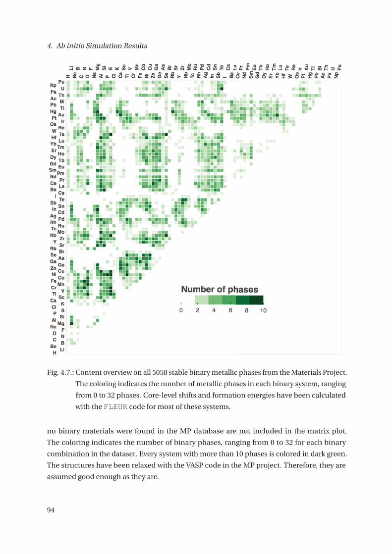
4. Ab initio Simulation Results
Fig. 4.7.: Content overview on all 5058 stable binary metallic phases from the Materials Project.
The coloring indicates the number of metallic phases in each binary system, ranging
from 0 to 32 phases. Core-level shifts and formation energies have been calculated
with the FLEUR code for most of these systems.
no binary materials were found in the MP database are not included in the matrix plot.
The coloring indicates the number of binary phases, ranging from 0 to 32 for each binary
combination in the dataset. Every system with more than 10 phases is colored in dark green.
The structures have been relaxed with the VASP code in the MP project. Therefore, they are
assumed good enough as they are.
94

4.2. Material Screening: Creating a Core-Level Shift Database
The structures are not further tested within this work to be completely force relaxed or
if their cell parameters are optimal, since uncertainties on chemical shifts from a 1-2 %
lattice constant mismatch is rather insignificant compared to other uncertainties [257]. Also
checking this more carefully would increase the number of SCF to be run within and therefore
the run time of this project by a factor 10-40.
In order to calculate initial-state core-level shifts for these binary structures, elemental
crystal structure references are also required. For this all 1271 non unique elemental crystal
structures at normal pressure were extracted from the ICSD.
To reach high accuracy in the core-level shifts, the same FLAPW parameters have to be
used for the reference calculation and the respective element in the compound. For this an
FLAPW parameter set was determined which would work for nearly all of the compounds.
This parameter set was fixed per element and is displayed in a periodic table plot in Fig. 4.8
including fixed electronic configurations with local orbitals. All compounds with f elements
or containing elements to have likely magnetic moments among others Fe, Co, Ni, Cr, Mn for
which FLEUR switches magnetism on per default, are calculated with collinear magnetism.
All calculations are performed with the core tail correction, spin-orbit coupling included and
the normal relativistic core solver of FLEUR, not the fully relativistic core solver. Therefore,
magnetism does not lead to further fine splittings of core levels. The coloring of the periodic
table plot has the same color scheme and scale as in Fig. 4.8 and corresponds to the muffin-tin
radii values. The muffin-tin radii were selected such that they work for most structures in
the binary and elemental data set. Depending on the element this choice corresponds to a
muffin-tin radius for the light elements within one standard deviation and for the 4f and 5f
elements up to six standard deviations of the default muffin-tin parameters of the OQMD
structure set in Fig. 4.8.
The number of grid points within the muffin-tin spheres was fixed for all systems to 981
points. The grid spacing dx , and the basis cutoff parameters �max, kmax were not fixed, but
determined by inpgen. The resulting distributions of �max and kmax for the binary metals
is shown in Fig. 4.9 on a logarithmic scale. The �max for most atom-types is like for the
OQMD structure set 6, 8 and mostly 10. The kmax distribution for the metals with fixed rMT is
much more narrow as for the OQMD set. Values for kmax range from 3.2 a0−1 to 7 a0
−1 with
98.9 % of the systems having a cutoff below 5 a0−1 and 70.4 % having a kmax smaller than
4 a0−1, which is quite reasonable. The small amount of systems with kmax values larger than
5 a0−1 correspond again to small rMT like for the elements H, O, N, C. As the muffin-tin radii
were fixed, and �max is not much varied by inpgen the basis set size cutoff relationship for
matching the basis function on the muffin-tin boundaries is less flexible.
The results for the matching criterion from equation 4.1 is shown in Fig. 4.10 as a logarithmic
95

4. Ab initio Simulation Results
Fig.4.8.:T
he
cho
senm
uffi
n-tin
radii,electro
nic
con
figu
ration
and
localo
rbitals
for
allelemen
tsis
disp
layedin
ap
eriod
ictab
le.
Th
isp
arameter
setw
asap
plied
inth
escreen
ing
with
FLEUR
of
the
stable
bin
arym
etallicp
hases
from
the
Materials
Pro
ject.Th
eco
lorin
go
fthe
elemen
tsin
dicates
the
mu
ffin
-tinrad
ius
and
the
colo
rscale
isco
mp
arable
toFig.4.3.
.
96

4.2. Material Screening: Creating a Core-Level Shift Database
distribution along side a logarithmic distribution for the resulting k-point density per atom-
type. Most of the system have a value below 1.0 meaning they have more basis function inside
the spheres than there are basis functions in the interstitial. Larger difference in muffin-tin
radii between elements lead to matching criterion values far away from 1. For the OQMD set
before this was different, the criterion for the inpgen defaults was always larger then one. The
difference comes from fixing the Muffin-tin radii. This shows that one should be more careful
when fixing muffin-tin radii of elements if the basis cutoffs are not flexible enough per default.
The K-point meshes were chosen as Monkhorst packs [275] such that the reciprocal spatial
K-point distance is at least 0.2 Å−1 in each spatial direction. The resulting number of K-points
per atom-type in the irreducible wedge of the Brillouin zone is shown in Fig. 4.10b. Overall
this value varies over a wide range.
(a) (b)
Fig. 4.9.: Two logarithmic histograms showing the basis cutoff choices determined byinpgen
for the binary structure set. In (a) the distribution of the radial basis cutoff �max shows
that �max is either 6,8, or 10. The distribution of the cutoff for the plane wave basis
kmax is shown in (b). It varies from 3.2 a0−1 to 7 a0
−1, while 98.9 % of the systems
have a cutoff below 5 a0−1 and 70.4 % have a kmax smaller than 4 a0
−1.
Now, that the FLAPW parameter set is fixed, one shot SCF workflows are launched on all
the elemental crystal structures without relaxing the crystal structures. Out of these 1271
elemental SCF simulations 1114 did succeed. The elemental structures with the lowest total
energy per atom are used farther as references in the core-level shift and for the formation
enthalpy calculations of the binary structures. In the first round of the binary structures a
initial-state workflow was run on the 4702 crystal structures containing less than 35 atoms,
the others 356 structures contain more then 35 atoms.
For the SCF runs on the small structures the maximum wall-time limit was 20 hours and a
maximum of 240 iterations in the self-consistency cycle is allowed. The maximum allowed
97

4. Ab initio Simulation Results
(a) (b)
Fig. 4.10.: In (a) the criterion for matching at the muffin-tin boundaries for the chosen FLAPW
parameters of the binary metallic structure set is shown. It is optimal if the basis
cutoff for the interstitial times the muffin-tin radius of atom-type α is approximately
equal to the cutoff for the muffin-tin basis. Values much large than one or lower
than one, might lead to matching problems in the FLAPW method. The coloring
indicates the differences in muffin-tin radii in the structure. In (b) the resulting
number of K-points per atom-type from the chosen K-point density of 0.2 Å−1 for the
structures is shown. It is an important convergence parameter in DFT calculations.
computational resources per SCF were 10 nodes on the JURECA supercomputer [276]. Though
for most of the small systems the SCF workflow decided to use one compute node. From the
4702 small binary systems 29 (0.6%) failed due to inpgen. 171 (3.6%) systems failed with
some FLEUR error message, 67 (1.4%) failed due to other causes. The most common FLEUR
failures include an unphysical or broken potential which results in a ’differ’ error message.
From the non-failed simulation subset not every charge density converged.
In Fig. 4.11 the convergence endpoints of the charge density distance and the total energy
difference to the previous iteration on a logarithmic scale are shown for all 4435 binary
systems and all 1114 elemental systems. 73.86 % (withing the green box of Fig. 4.11) of all
FLEUR calculations reached the convergence cutoff criterion of 5 ·10−6 me/a−30 in less then
240 iterations or before running out of granted wall time. The convergence rate of 86.22 % for
the 3127 non-magnetic systems is better than the convergence rate of 57.93 % for the 2422
magnetic calculations. 9.93 % of the systems did not converge at all (charge distance >0.5
me/a−30 , black box of Fig. 4.11), with 82.6 % of these being magnetic calculations. Partially
converged systems amount to the other 16.20 % of all systems while non magnetic calculations
amount to 37.3 % of the partially converged systems. This should be seen with care and as a
snapshot in time. There was a hybrid parallelization resource requesting mistake leading to a
98

4.2. Material Screening: Creating a Core-Level Shift Database
Fig. 4.11.: Charge density and total energy convergence behavior of FLEUR calculations on
4435 binary metals from the Materials Project and 1114 elemental structures from
the ICSD. Most of the non magnetic (blue) and magnetic systems (red) converge in
both quantities (green box). Around 16 % of the systems did converge partial and
10 % not at all (black box). Due to a computational resource assignment mistake,
the ’real’ converge rate is expected to be much better. Only 5 % of the systems did
not converge within 240 iteration. The area of the markers indicate the number of
iterations run.
99
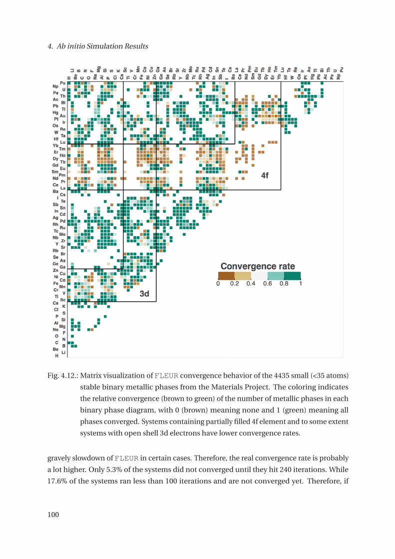
4. Ab initio Simulation Results
Fig. 4.12.: Matrix visualization of FLEUR convergence behavior of the 4435 small (<35 atoms)
stable binary metallic phases from the Materials Project. The coloring indicates
the relative convergence (brown to green) of the number of metallic phases in each
binary phase diagram, with 0 (brown) meaning none and 1 (green) meaning all
phases converged. Systems containing partially filled 4f element and to some extent
systems with open shell 3d electrons have lower convergence rates.
gravely slowdown of FLEUR in certain cases. Therefore, the real convergence rate is probably
a lot higher. Only 5.3% of the systems did not converged until they hit 240 iterations. While
17.6% of the systems ran less than 100 iterations and are not converged yet. Therefore, if
100

4.2. Material Screening: Creating a Core-Level Shift Database
most of these systems still converge the overall non-converge rate could be around 9% only
instead of 26.14%. But this is still unclear until these systems are rerun with if necessary more
resources. Collinear magnetic calculations are expected to be harder to converge, since the
spin density has to be converged in addition to the charge density. Also the non-convergence
of magnetic systems might correlate with the choice of the starting magnetic configuration as
well as the fact that many of these systems contain open 4f shells.
A more detailed picture on which of the 4435 binary systems the SCF workflow managed to
converge and which not, is gained from the matrix plot in Fig. 4.12. For each binary phase
diagram the relative convergence rate from 0 to 1 is depicted. While a rate of 1 (green) means
that the charge density converged for all metal phases in the corresponding phase diagram,
a rate of 0 (brown) shows that no or a few phases converged. From this representation it
becomes apparent that there are mainly convergence problems with magnetic calculation of
the 4f systems with the chosen setup. The other cases are more distributed over all phases,
while systems with open 3d shells systems which are generally calculated magnetic show also
lower convergence rates. It is known in the literature that open 4f systems are challenging to
describe correctly in standard DFT, like converging to the right magnetic ground state [277].
Converging the spin-dependent charge density becomes challenging, since the 4f electrons
form localized bands close to the Fermi energy, resulting in an energy landscape with many
local minima. There are several approaches to treat open f systems. One way within DFT is
treating the f or d orbitals with the LDA+U method [254, 278, 279] to split them apart with an
occupational dependent energy contribution, or the LDA+HIA approach [280]. It is beyond
this work to automatize these approaches and to develop checks if the simulations converged
into a physical accurate minimum. From the 1637 binary phase diagrams seen in the matrix
visualization of Fig. 4.12 for 55% the diagram all phases converged, forming probably good
data sets.
101
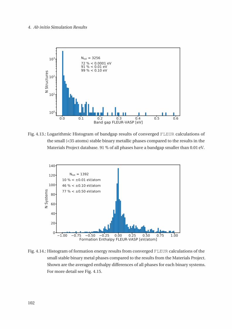
4. Ab initio Simulation Results
Fig. 4.13.: Logarithmic Histogram of bandgap results of converged FLEUR calculations of
the small (<35 atoms) stable binary metallic phases compared to the results in the
Materials Project database. 91 % of all phases have a bandgap smaller than 0.01 eV.
Fig. 4.14.: Histogram of formation energy results from converged FLEUR calculations of the
small stable binary metal phases compared to the results from the Materials Project.
Shown are the averaged enthalpy differences of all phases for each binary systems.
For more detail see Fig. 4.15.
102
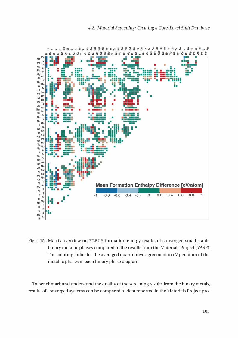
4.2. Material Screening: Creating a Core-Level Shift Database
Fig. 4.15.: Matrix overview on FLEUR formation energy results of converged small stable
binary metallic phases compared to the results from the Materials Project (VASP).
The coloring indicates the averaged quantitative agreement in eV per atom of the
metallic phases in each binary phase diagram.
To benchmark and understand the quality of the screening results from the binary metals,
results of converged systems can be compared to data reported in the Materials Project pro-
103

4. Ab initio Simulation Results
(a) (b)
(c) (d)
Fig. 4.16.: A birds-eye view on core-level shifts of the chemical environments of the converged
binary metals is presented in these histograms. The distribution in histogram (a)
contains all main-line core-level shifts for each atom-type. 15 % of all atom-types
have a chemical shift smaller then 0.1 eV. The other three histograms (b, c, d) show
the core-level shift contributions of the main spectral lines of certain elements. Be
1s core-level shifts (b) are most of the time positive with mostly lie between 0.5 eV
and 1.5 eV. For W (c) the 4f doublet shifts show a wide spread, though there are not
so many data points. The Ti 2p doublet shifts mostly to lower binding energy values.
as is shown in (b).
duced with the VASP DFT program. First, it is checked if all metallic systems predicted by
VASP have no bandgap in the FLEUR simulations. The bandgap difference for all converged
structures is shown in the logarithmic histogram in Fig. 4.13. For 91 % of the 3256 structures
the codes agree well and the FLEUR bandgap is smaller than 0.01 eV, where 99% of the struc-
104

4.2. Material Screening: Creating a Core-Level Shift Database
tures have a FLEUR bandgap smaller than 0.1 eV. The other systems with a small bandgap
should be investigated in detail. After confirming that no crude mistake was made one could
find out if the change was because of the inclusion of spin-orbit coupling, or differences
between an all-electron and a pseudo-potential method.
To gain more insight, we compare a more complex quantity like the enthalpy of formation,
which value and accuracy depends on DFT simulations on three different structures, like
the initial-state core-level shifts. Here systematic errors can occur, if for example the chosen
reference structures are not the same. The matrix plot in Fig. 4.15 displays the difference in
the enthalpy of formation per atom for each binary system averaged over all metallic phases
in it. The formation energies for binaries with gases like H, N, O, Cl and so on are expected to
be wrong, because they are not calculated so simple, but need correction terms [119]. From
this matrix visualization one can spot the elements where the references is likely problematic
since most binary systems containing that element have a large deviation from the VASP
results, like for Pa, Ni and elements with open 4f shells. The information in the matrix of Fig.
4.15 is summed up by a histogram in Fig. 4.14. From the histogram it becomes clear that the
spread of the distribution is quite large only around 11 % of all systems agree with vasp within
0.01 eV per atom. Half of the systems give the same enthalpy as VASP within 0.1 eV per atom.
The 4435 metals systems correspond to 23939 main line core-level shifts for different atom-
types and structures and 208456 calculated core-level shifts in total. The 3256 converged
systems yield a dataset of 15936 unique main line core-level shifts for different atom-types
and structures with 137651 core-level shifts in total. For the unique main-line core-level shifts
this amount is more than twice the number of unique main-line core-level shifts contained
in the NIST XPS database [90]. An overview of all the main-line chemical shifts of binary
metals is shown in Fig. (a) of Fig. 4.16. Metallic phases often have very small core-level shifts
(84% are smaller than ±1 eV), but they can also be larger than ±2 eV for certain chemical
environments. Overall, the distributions mean is around 0. and 15% of all core-level shifts
are smaller than ±0.1 eV making these chemical environments indistinguishable within the
experimental uncertainties from the elemental bulk material. The small visible peaks of
core-level shifts of around 4 eV is an artifact of a wrong reference value for the elements Pa,
Tb, N, O and F. For different elements the distribution of the chemical shifts can be totally
different. In the sub figures (b,c,d) of Fig. 4.16 the chemical shift distributions are shown for
the Be, W and Ti main core-level lines. Chemical shifts of 1s states of Be atom-types are likely
to have a positive shift and the distribution peaks below 1 eV. In contrast the Ti 2ps rather
have a negative chemical shift with a large spread peaking slightly below −0.5 eV. For the W
4f shifts the statistics is not very good, but so far they show a wide spread and contain shifts
towards smaller binding energies as well as shifts towards larger binding energies.
105
4. Ab initio Simulation Results
To benchmark and understand the quality of the screening results from the binary metals
and the quality of the applied core-level shift method, simulated core-level shifts are compared
to the experimental literature. For this the XPS NIST database [90] was mined and the overlap
to the screening materials determined by chemical formula. Therefore, the crystal structure or
even phase content might differ between my results and experiments. From the 6300 unique
chemical formulas in NIST the overlap to the screened non failed 4435 binary metals was 62
materials, of which 45 simulations converged. The 45 materials are: AgF, AgMg, Al3Ti, AlB2,
AlMn, AlNi, AlTi, Au2Ti, Au3Cu, AuCu3, AuMg, AuTe2, Bi2Mg3, CdO, CePd3, Co9S8, CoSi2, Cu2S,
CuS, Fe3Si, FeSi2, GaNi, GaNi3, HgS, HgTe, In3Ni2, InNi3, InSb, MnN, MnSe, MnTe, MnZn,
MoN, MoSi2, NbPd2, NbS2, NbSe2, NdPd3, Ni2Ta, NiTi, Pd2Ta, Pd3Sm, Pd3Ti, PdSc and Pt2Si.
These materials have entries for 133 core-level shifts in NIST, partially reported directly in the
experimental literature. These 133 core-level shifts are compared to the screening results in
Fig. 4.17.
The experimental data is quite uncertain and there are known problems with numerical XPS
databases [247, 248]. The applied initial-state method with one shot SCF FLEUR calculations
seems to work quite well for the prediction of small chemical shifts in metals between −1 eV
and 1 eV. It seems so far to fail to predict larger core-level shifts in metals right. But with such
little data and such a spread in the data it is impossible to conclude that the method predicts
metallic shifts well within high accuracy. For a better evaluation of the quality of the data one
should compare directly to high resolution experimental spectra, like it is done in section 4.3.
A sum up of resources needed for this small prove of concept screening project is given in
Tab. 4.2. Such a small project is not a challenge for AiiDA, the database with 0.5 million nodes
is not large yet, but in this AiiDA version with the Django backend the size of the database
is already quite large, which is seen in the time needed for queries on the database. The
simulations took 2 weeks to execute with the throughput capabilities available to a single
user on JURECA. Due to a mistake in resource requesting for hybrid jobs FLEUR ran slower
than expected and the computational time used is probably a lot larger than what would
be needed. With a better performance prediction of FLEUR such bottlenecks or suboptimal
usage might become detectable. All the files which were stored for longterm from the project
took around 1 TB of disk space. Where the ’out.xml’ files and ’last_cdn.hdf’ take each around
120 GB. This one TB of data could be reduced by further deleting, or grouping smaller files.
Keeping only the ’out.xml’ files and deleting the ’out’ files. Also removing some iterations
from the output files or the eigenvalue write outs can decrease the storage footprint further.
106

4.2. Material Screening: Creating a Core-Level Shift Database
Fig. 4.17.: Comparison of the screening results with overlapping entries of the NIST XPS
[90] database. In (top) 133 core-level shifts reported in the literature (blue) and
computed from literature reported binding energies (red) are compared to the
calculation results with the FLEUR code. In (bottom) a comparison of 55 experi-
mental mean values for core-level shifts from NIST XPS entries of 45 binary metallic
compounds is shown. Different core-level types differ in color. Data points repre-
sent mean values from the NIST database, with the error bar being the standard
deviation on the mean value or 0.6 eV for single values.
107

4. Ab initio Simulation Results
Quantity Value Comment
Elemental structures from ICSD 1271 1132 < 21 atoms, 157 failed
Number of metals from MP 5058 355 contain >35 atoms
Number of initial-state workflows 4702
Number of SCF workflows run 5973
Total Convergence rate 68.6% <=5.0−6 me/a30, real prob +15%
Total Non-convergence rate 24.3% >5.0−6 me/a30 within resources
Total Failure rate 7.1% various causes
Size out.xml files 120 GB total sum
Total disk space (repo) 990 GB including other simulations
Total disk space (repo) tar.gz 295 GB
i-nodes on disk 2.5 mio. will be less with AiiDA > 1.0
FLEUR version MaX 2 release + with included bugfixes
AiiDA version 0.12.3 without rabbitMQ
AiiDA database schema Django no json filed support yet
AiiDA-FLEUR version 0.6.3 still on python 2
Nodes in AiiDA database 0.5 mio. less overhead with AiiDA > 1.0
AiiDA database size on disk 34 GB with json filed might become smaller
Total computational time used 800K core/hours >80% wasted in wrong parallelization
Tab. 4.2.: This table sums up information of the small screening project of the metallic binaries
from the Materials Project. Core-level shifts of these structures were calculated The
resulting files from this project for long time storage take about 1 TB of disk space
if uncompressed. A large contribution comes from the number of files (2.5 mio.
i-nodes). The total execution time of the project was 2 weeks.
108
4.2. Material Screening: Creating a Core-Level Shift Database
4.2.1. Data Quality and Robustness
With powerful frameworks like AiiDA it becomes very easy to produce a lot of data with
different quality, precision and even trash. AiiDA itself already tackles this problem at the
core by storing the full provenance enabling the implementation of quality checks in work-
flows or on the database itself, but overall the user has the responsibility. In the electronic
structure community there have been efforts in recent years [120, 268] to develop methods
for quantifying uncertainties and accuracies between different DFT packages, methods and
experiment. In this work this broader issue was not touched, but the convergence behavior of
the relevant quantities was investigated or known. Through this knowledge I believe most of
the individual calculations to be accurate enough.
One should be skeptical about high-throughput results until quality measures are in place,
since there can be systematic errors or biases in calculations or in on top data analysis. For
example treating a certain element not in the right way, i.e wrong structure, or electronic
starting configuration and so forth, would cause a systematic uncertainty. One source of
systematic uncertainty for formation energies and core-level shifts is how the elemental
reference structure was chosen. Calculating every elemental structure in the ICSD and using
the one with the lowest energy per atom as a reference may not be the best choice. Structures
with convergence problems were just excluded, which is certainly not optimal. For example
there was a systematic uncertainty found for the reference of Beryllium. Systematic errors
from data analysis on top of calculations can be corrected without rerunning all simulations,
as long as there is no problem with the individual runs. In this context it might make sense to
keep the data analytics part as separate from the calculations and modular as possible.
4.2.2. Conclusion and Outlook Screening
With a small prove of principle project of over 5500 crystal structures it was demonstrated
that high-throughput calculation with the FLAPW method and the FLEUR code are possible.
The results of the project, the performance of FLEUR (MPI develop version 11.2018) and the
SCF workflow are a snapshot in time and should not be generalized so easily. The stability/ro-
bustness of inpgen, the FLEUR program and the workflow, can still be improved to decrease
the failure rate of simulations, which was in total for this project around 7%. Errors need to
be properly caught by FLEUR or the AiiDA-FLEUR package to avoid any loss of simulation
data due to other failures. If certain failures can not be avoided but corrected for the workflow
should do so.
Small mistakes can have large consequences in a high-level environment. Due to a one line
hybrid parallelization job script mistake over 80 % of the computing time was wasted, making
109

4. Ab initio Simulation Results
the runtime performance and convergence failure rate way worse than they are in reality.
To archive higher convergence rates of systems and more physical simulation results more
expert knowledge of the FLAPW method like from [81] has to be included in the SCF workflow.
This includes quality checks for FLAPW input parameters and output results, handling of
FLEUR errors where possible, predicting the runtime ofFLEUR and choosing a suitable hybrid
parallelization for a given system. The usage of other mixing and preconditioning strategies
in the workflow may improve convergence speed. Better starting points and handling of
magnetic systems might improve convergence rates of magnetic systems. Automation of
LDA+U and other features like smarter local orbital choice will help to improve the description
of insulators and open shell f-elements. For physical accurate results measures for fidelity
have to be found and implemented. Getting a converged result is the first step, deciding if this
result is physical meaningful the next step.
The main line core-level shifts from the 4435 converged systems provide additional refer-
ence data for nearly as many systems as are stored in the NIST XPS database and the number
of main line core-level shifts is more than double the number of core-level shifts in NIST XPS
database. Though not all data is to be trusted as pointed out. As first trustworthy data set one
can start with the data subset agreeing well with VASP calculations. What a complete set of
core-level shift data of a material system can be used for is demonstrated in the following
section.
4.3. Example: Fusion Relevant Materials
In Cadarache, Southern France, the so far largest nuclear fusion experiment is currently under
construction. The International Thermonuclear Experimental Reactor (ITER, lat. ’the way’)
is a tokamak reactor type [281]. The first plasma ignition of ITER is planned to happen in
2025. The way towards the final goal of an industrial fusion reactor for mankind’s sustainable
CO2 free energy needs is still long (see the eurofusion road map to 2050 [281, 282]). From the
insights gained from ITER an even larger industrial prototype reactor (DEMO) is planned to
be build. A fusion reactor is a very complex machine (for an impression see Fig. 4.18), posing
profound challenges to science and engineering.
One fundamental aspect is the plasma-wall interaction [283] of the inner fusion reactor
vessel and designing materials for withstanding the operation conditions of ITER, DEMO
and reactors beyond. One material criterion is a low half-life for all activated isotopes and
elements in the decay chain. For ITER the inner plasma-facing wall (’the blanket’, 600 m2,
see Fig. 4.19) will be coated with the light metal beryllium, because it features a rather high
melting point and low tritium absorption, which is important for radiation safety issues. In
110
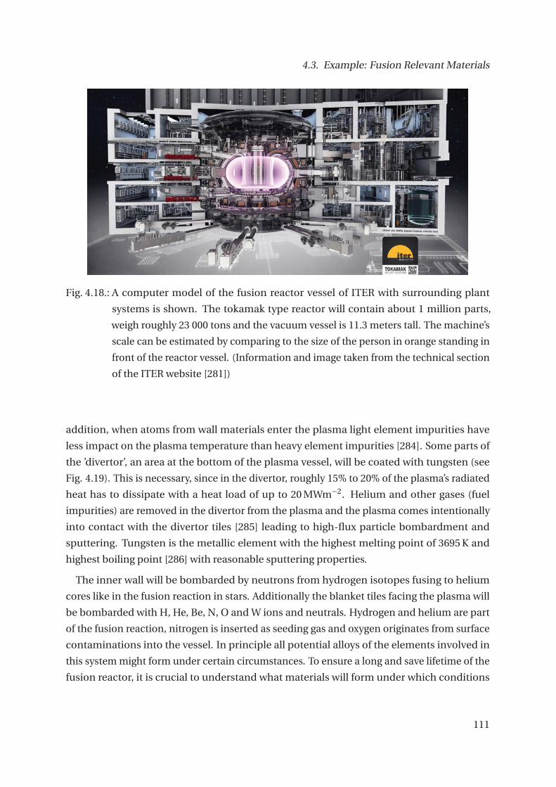
4.3. Example: Fusion Relevant Materials
Fig. 4.18.: A computer model of the fusion reactor vessel of ITER with surrounding plant
systems is shown. The tokamak type reactor will contain about 1 million parts,
weigh roughly 23 000 tons and the vacuum vessel is 11.3 meters tall. The machine’s
scale can be estimated by comparing to the size of the person in orange standing in
front of the reactor vessel. (Information and image taken from the technical section
of the ITER website [281])
addition, when atoms from wall materials enter the plasma light element impurities have
less impact on the plasma temperature than heavy element impurities [284]. Some parts of
the ’divertor’, an area at the bottom of the plasma vessel, will be coated with tungsten (see
Fig. 4.19). This is necessary, since in the divertor, roughly 15% to 20% of the plasma’s radiated
heat has to dissipate with a heat load of up to 20 MWm−2. Helium and other gases (fuel
impurities) are removed in the divertor from the plasma and the plasma comes intentionally
into contact with the divertor tiles [285] leading to high-flux particle bombardment and
sputtering. Tungsten is the metallic element with the highest melting point of 3695 K and
highest boiling point [286] with reasonable sputtering properties.
The inner wall will be bombarded by neutrons from hydrogen isotopes fusing to helium
cores like in the fusion reaction in stars. Additionally the blanket tiles facing the plasma will
be bombarded with H, He, Be, N, O and W ions and neutrals. Hydrogen and helium are part
of the fusion reaction, nitrogen is inserted as seeding gas and oxygen originates from surface
contaminations into the vessel. In principle all potential alloys of the elements involved in
this system might form under certain circumstances. To ensure a long and save lifetime of the
fusion reactor, it is crucial to understand what materials will form under which conditions
111
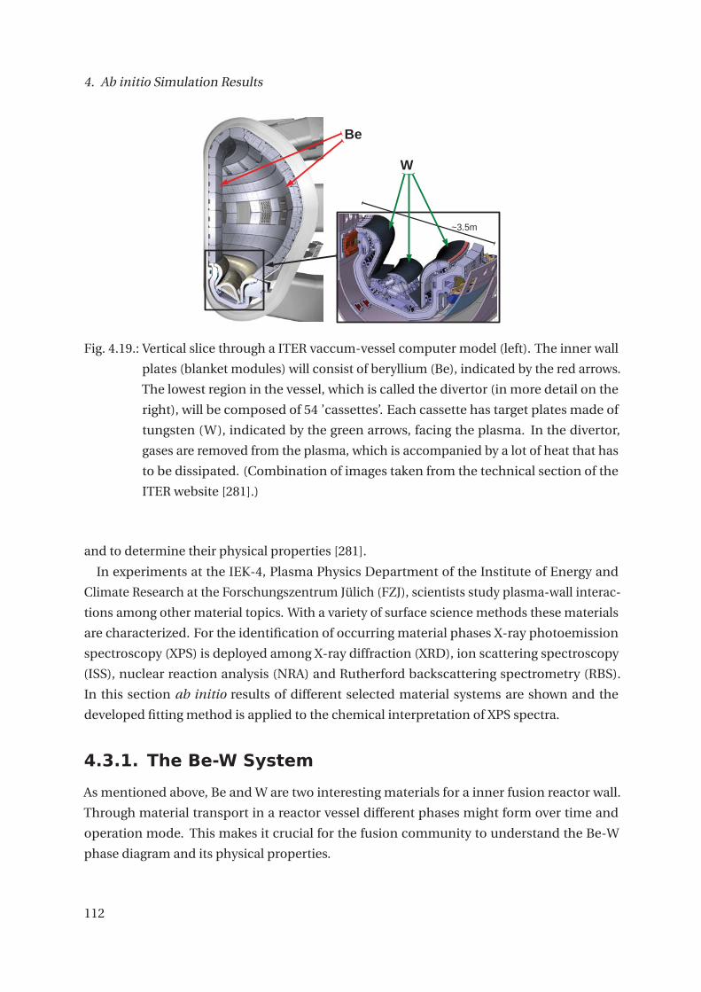
4. Ab initio Simulation Results
Fig. 4.19.: Vertical slice through a ITER vaccum-vessel computer model (left). The inner wall
plates (blanket modules) will consist of beryllium (Be), indicated by the red arrows.
The lowest region in the vessel, which is called the divertor (in more detail on the
right), will be composed of 54 ’cassettes’. Each cassette has target plates made of
tungsten (W), indicated by the green arrows, facing the plasma. In the divertor,
gases are removed from the plasma, which is accompanied by a lot of heat that has
to be dissipated. (Combination of images taken from the technical section of the
ITER website [281].)
and to determine their physical properties [281].
In experiments at the IEK-4, Plasma Physics Department of the Institute of Energy and
Climate Research at the Forschungszentrum Jülich (FZJ), scientists study plasma-wall interac-
tions among other material topics. With a variety of surface science methods these materials
are characterized. For the identification of occurring material phases X-ray photoemission
spectroscopy (XPS) is deployed among X-ray diffraction (XRD), ion scattering spectroscopy
(ISS), nuclear reaction analysis (NRA) and Rutherford backscattering spectrometry (RBS).
In this section ab initio results of different selected material systems are shown and the
developed fitting method is applied to the chemical interpretation of XPS spectra.
4.3.1. The Be-W System
As mentioned above, Be and W are two interesting materials for a inner fusion reactor wall.
Through material transport in a reactor vessel different phases might form over time and
operation mode. This makes it crucial for the fusion community to understand the Be-W
phase diagram and its physical properties.
112

4.3. Example: Fusion Relevant Materials
Fig. 4.20.: Convex-hull diagram of the Be-W system. While the Be2W phase is energetically
most stable the Be22W is predicted to be slightly metastable with 25 meV distance
from the hull. For all results the PBE functional was used. There may be an ad-
ditional stable BeW phase predicted by DFT (AFLOWlib [56]), which is currently
experimentally unconfirmed.
There are three experimentally known phases Be2W, Be12W and Be22W in the literature [287]
and included in the metal database of this project. In addition, there may be a theoretical
phase of BeW (predicted by AFLOWlib with VASP) which is experimentally not reported yet.
The Be-W systems was investigated with DFT for various aspects in [288–291]. The most stable
W phase has a basic centered cubic (bcc) symmetry and Be crystallizes in the hexagonal close-
packed (hcp) structure. The convex hull diagram in Fig. 4.20 from our results makes it clear
that Be2W is the most stable phase predicted by DFT in terms of enthalpy of formation per
atom for the Be-W system. Whereas, the reported experimental crystal structure of the Be22W
system lies, at least for the PBE functional and the used Be and W crystal structure references,
25 meV above the convex-hull construction. This is in agreement with the experimental
observation that it seems harder to synthesize a sample with Be22W than the other two stable
phases [292, 293]. Be12W is predicted to be stable and does not lie on the connecting hull
line from Be2W and Be. Hence, making from an energetic viewpoint a pure phase preferable
over mixed phases at the 12:1 stoichiometry. This behavior is different for Be12Ti and Be12Ta
113

4. Ab initio Simulation Results
which lie on the hull line as will be discussed in other subsections. Overall, our formation
energies are in agreement with findings from other DFT simulations from various databases.
The findings from others are included in Fig. 4.20.
Fig. 4.21.: Equation of states calculated with the FLEUR code for all known stable Be-W sys-
tems. The bravais matrix was scaled and not the cell optimized under constraint
volume. All energy volume curves are calculated using the PBE functional.
In order to check the quality of the experimental crystal structures and if they are well
described by the PBE functional a Birch-Murnaghan equation of states for each phase was
calculated with FLEUR and is shown in Fig. 4.21. The unit cells are scaled without optimizing
the lattice parameters for each volume. The resulting ground-state volumes from a Birch-
Murnaghan fit of Be22W and Be12W is 2% and 4% underestimated by DFT with the PBE
functional. For Be2W the ground-state volume is slightly overestimated by 1%. The equation
of states results are summed up with the enthalpy of formation in Tab. 4.3.
Initial-state core-level shifts of the Be-W system were calculated. These core-level shifts
and the number of corresponding electrons in the chemical environment are listed in Tab. 4.4.
Core-level shifts on these systems calculated with an older version of the FLEUR code were
reported in [257]. From the core-level shift and the corresponding atom-type information
theoretical spectra can be constructed as proposed in section 3.2. Such theoretical ideal XPS
spectra for the Be 1s and W 4f binding energy region are displayed in Fig. 4.22 for all Be-W
114
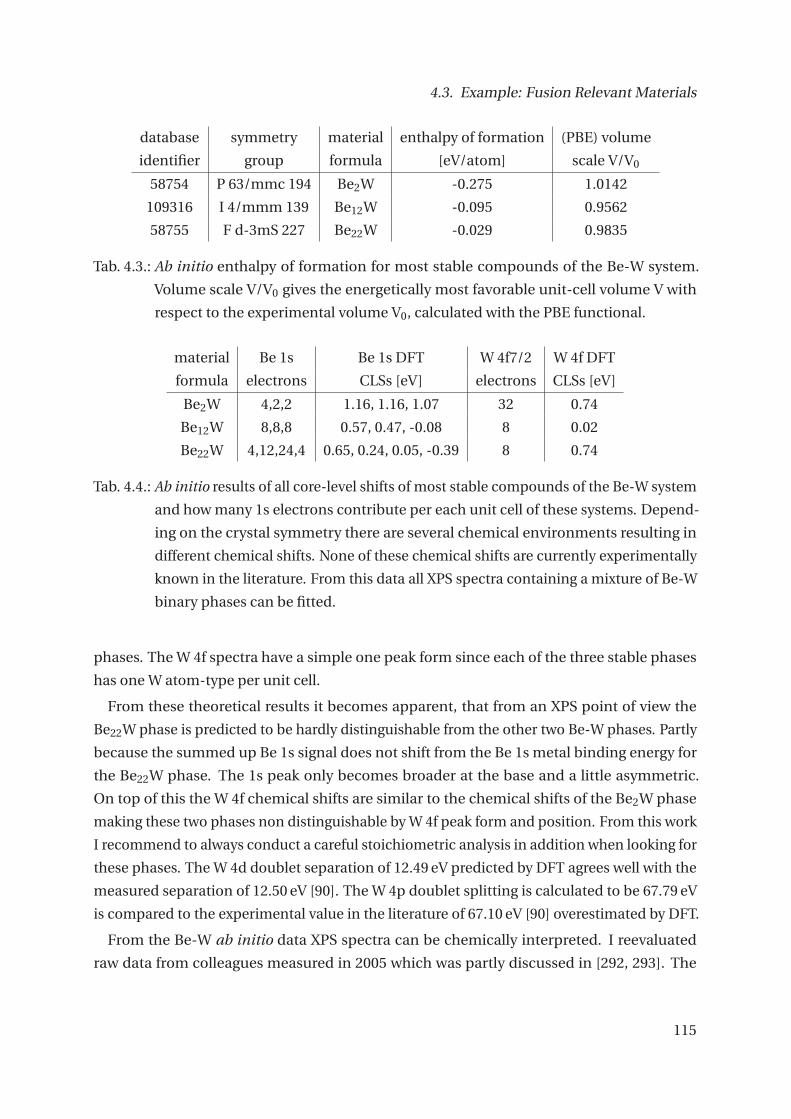
4.3. Example: Fusion Relevant Materials
database symmetry material enthalpy of formation (PBE) volume
identifier group formula [eV/atom] scale V/V0
58754 P 63/mmc 194 Be2W -0.275 1.0142
109316 I 4/mmm 139 Be12W -0.095 0.9562
58755 F d-3mS 227 Be22W -0.029 0.9835
Tab. 4.3.: Ab initio enthalpy of formation for most stable compounds of the Be-W system.
Volume scale V/V0 gives the energetically most favorable unit-cell volume V with
respect to the experimental volume V0, calculated with the PBE functional.
material Be 1s Be 1s DFT W 4f7/2 W 4f DFT
formula electrons CLSs [eV] electrons CLSs [eV]
Be2W 4,2,2 1.16, 1.16, 1.07 32 0.74
Be12W 8,8,8 0.57, 0.47, -0.08 8 0.02
Be22W 4,12,24,4 0.65, 0.24, 0.05, -0.39 8 0.74
Tab. 4.4.: Ab initio results of all core-level shifts of most stable compounds of the Be-W system
and how many 1s electrons contribute per each unit cell of these systems. Depend-
ing on the crystal symmetry there are several chemical environments resulting in
different chemical shifts. None of these chemical shifts are currently experimentally
known in the literature. From this data all XPS spectra containing a mixture of Be-W
binary phases can be fitted.
phases. The W 4f spectra have a simple one peak form since each of the three stable phases
has one W atom-type per unit cell.
From these theoretical results it becomes apparent, that from an XPS point of view the
Be22W phase is predicted to be hardly distinguishable from the other two Be-W phases. Partly
because the summed up Be 1s signal does not shift from the Be 1s metal binding energy for
the Be22W phase. The 1s peak only becomes broader at the base and a little asymmetric.
On top of this the W 4f chemical shifts are similar to the chemical shifts of the Be2W phase
making these two phases non distinguishable by W 4f peak form and position. From this work
I recommend to always conduct a careful stoichiometric analysis in addition when looking for
these phases. The W 4d doublet separation of 12.49 eV predicted by DFT agrees well with the
measured separation of 12.50 eV [90]. The W 4p doublet splitting is calculated to be 67.79 eV
is compared to the experimental value in the literature of 67.10 eV [90] overestimated by DFT.
From the Be-W ab initio data XPS spectra can be chemically interpreted. I reevaluated
raw data from colleagues measured in 2005 which was partly discussed in [292, 293]. The
115

4. Ab initio Simulation Results
(a) Be2W, Be 1s (b) Be2W, W 4f
(c) Be12W, Be 1s (d) Be12W, W 4f
(e) Be22W, Be 1s (f ) Be22W, W 4f
Fig. 4.22.: Theoretical single-phase XPS spectra of Be 1s and W 4f from the three stable Be-
W alloys Be2W (a), Be12W (b), and Be22W (c). The spectra are constructed from
the ab initio chemical shifts and the atom-type information in Tab. 4.4 of one
computational unit cell. All Voigt profiles have a Lorentzian FWHM of 0.1 eV and a
Gaussian FWHM of 0.43 eV. Binding energies of the elemental reference are marked
with horizontal lines.
116

4.3. Example: Fusion Relevant Materials
(a) Be 1s spectra (b) W 4f spectra
Fig. 4.23.: Experimental raw data from a depth analysis with sputter XPS of annealed W on
Be. Label positions indicate calculated spectral positions of Be-W alloys. On the
left a Be 1s spectra series is shown with different Ar fluxes (from bottom to top).
Vertical lines mark Be 1s binding energies from the literature for Be bulk and for
beryllium oxide. To show the shifting of spectral, peaks two additional lines with
1 eV difference are added. The spectra series on the right shows high-resolution
XPS spectra in the W 4f binding energy region for the same Ar fluxes as on the left.
Vertical lines mark the W 4f binding energy positions of W bulk.117

4. Ab initio Simulation Results
XPS data was not completely understood at that time. A few hundred nanometer W were
evaporated onto a Be bulk sample. After annealing the sample the formation of a Be12W film
was concluded through RBS [292] and XRD [293] measurements. Furthermore, sputter XPS
and RBS measurements were performed [292], totaling 37 spectra each. The evaluation of
the 1 MeV proton RBS concluded a Be:W stoichiometry of 12:1 below the oxidized surface
with an information depth of at least 1μm for W [294]. In contrast the Be:W stoichiometry
determined from the W 4f and Be 1s XPS spectra area ratios corresponds in the ’alloy region’
only to 3.3:1. This mismatch of the stoichiometry between XPS and RBS is argued to arise
from preferential sputtering of Be over W and because XPS is more sensitive to the surface
region than RBS. In their work the Be 1s XPS spectra were fitted with three Gauss-Lorentz
functions, one for the ’oxid’ peak around 114.4 eV and one named ’metal’ and one named
’alloy’ with a constant shift of 0.51 eV.
While the stoichiometry determined from XPS was only 3.3:1 they still concluded that this
’alloy’ peak in the ’alloy region’ corresponds to Be12W as indicated by RBS. This, I now doubt
to be the case. At first sight it seems to agree well with the ab initio results for Be12W, since
the initial-state shifts of Be12W suggest that both peaks ’alloy’ and ’metal’ (from [292]) belong
to a clear Be12W spectrum within the 3μm thick film region. First, because the measured
shift of 0.51 eV in the publication [292] would agree with the mean shift of 0.52 eV of the two
shifted chemical environments of Be12W. Second, because the peak area ratio of the ’metal’
and ’alloy’ reported in figure 3 of the publication [292] is roughly 1:3 at the beginning of the
series and in the ’alloy’ region as is also the predicted ratio by DFT for the shifted and non
shifted components of pure Be12W.
But looking in detail at the raw XPS spectra data of Be 1s and W 4f shown in Fig. 4.23 the
picture for the chemical interpretation clearly changes. The raw data shows a clear drift of
the Be 1s spectrum over the sputter series (from bottom to top) of the ’alloy’ and ’metal’
peak together to lower binding energies by nearly 1.0 eV. This shift was corrected in the
original evaluation by keeping the Be 1s metal peak fixed. The W 4f spectra also clearly shift
with respect to W 4f bulk over the sputter series. Both observations can not be explained
theoretically by Be12W, which has no chemical shift in the W 4f core levels and the Be 1s
spectra are predicted to stay at the same binding energy as long the energy axis is calibrated
right throughout the experiment and no sample charging occurs. The BeO 1s signal which
would be expected to be at 113.7 eV [90] lies between 114.8 eV-115.0 eV, which might have
been their motivation for fixing the Be-O Be bulk Be difference to 3.0 eV and assuming a
charging effect. This amount to a 1.0 eV correction of the Be 1s binding energies.
With our evaluation method I can now clarify the chemical interpretation of this sputter
XPS series raw data without correcting the binding energy over this series by 1.0 eV. I have
118

4.3. Example: Fusion Relevant Materials
(a) Be 1s Spectrum 2 (b) W 4f Spectrum 2
(c) Be 1s Spectrum 16 (d) W 4f Spectrum 16
(e) Be 1s Spectrum 29 (f ) W 4f Spectrum 29
Fig. 4.24.: A representative subset of the sputter XPS spectra (data sets 2,16,29) on Be-W from
[292] is shown with component fits from ab initio data. In (a) a Be 1s spectrum at
the start of the sputtering is shown yielding only a contribution from Be12W. The
W 4f (b) can also be matched with Be12W only. The Be 1s spectrum in (c) can be
fitted with contributions from Be12W and Be2W while the component fit of the
corresponding W 4f doublet spectrum (d) can be fitted with solely Be2W. The fits in
(e,f) show that the spectra can also be fitted with a small contribution of Be12W in
the tail. 119
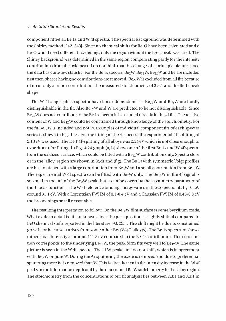
4. Ab initio Simulation Results
component fitted all Be 1s and W 4f spectra. The spectral background was determined with
the Shirley method [242, 243]. Since no chemical shifts for Be-O have been calculated and a
Be-O would need different broadenings only the region without the Be-O peak was fitted. The
Shirley background was determined in the same region compensating partly for the intensity
contributions from the oxid peak. I do not think that this changes the principle picture, since
the data has quite low statistic. For the Be 1s spectra, Be2W, Be12W, Be22W and Be are included
first then phases having no contributions are removed. Be22W is excluded from all fits because
of no or only a minor contribution, the measured stoichiometry of 3.3:1 and the Be 1s peak
shape.
The W 4f single-phase spectra have linear dependencies. Be22W and Be2W are hardly
distinguishable in the fit. Also Be12W and W are predicted to be not distinguishable. Since
Be22W does not contribute to the Be 1s spectra it is excluded directly in the 4f fits. The relative
content of W and Be12W could be constrained through knowledge of the stoichiometry. For
the fit Be12W is included and not W. Examples of individual component fits of each spectra
series is shown in Fig. 4.24. For the fitting of the 4f spectra the experimental 4f-splitting of
2.18 eV was used. The DFT 4f-splitting of all alloys was 2.24 eV which is not close enough to
experiment for fitting. In Fig. 4.24 graph (a, b) show one of the first Be 1s and W 4f spectra
from the oxidized surface, which could be fitted with a Be12W contribution only. Spectra close
or in the ’alloy’ region are shown in (c,d) and (f,g). The Be 1s with symmetric Voigt profiles
are best matched with a large contribution from Be2W and a small contribution from Be12W.
The experimental W 4f spectra can be fitted with Be2W only. The Be12W in the 4f signal is
so small in the tail of the Be2W peak that it can be covert by the asymmetry parameter of
the 4f peak functions. The W 4f reference binding energy varies in these spectra fits by 0.1 eV
around 31.1 eV. With a Lorentzian FWHM of 0.1-0.4 eV and a Gaussian FWHM of 0.45-0.8 eV
the broadenings are all reasonable.
The resulting interpretation to follow: On the Be12W film surface is some beryllium oxide.
What oxide in detail is still unknown, since the peak position is slightly shifted compared to
BeO chemical shifts reported in the literature [90, 295]. This shift might be due to constrained
growth, or because it arises from some other Be-(W-)O alloy(s). The Be 1s spectrum shows
rather small intensity at around 111.8 eV compared to the Be-O contribution. This contribu-
tion corresponds to the underlying Be12W, the peak form fits very well to Be12W. The same
picture is seen in the W 4f spectra. The 4f W peaks first do not shift, which is in agreement
with Be12W or pure W. During the Ar sputtering the oxide is removed and due to preferential
sputtering more Be is removed than W. This is already seen in the intensity increase in the W 4f
peaks in the information depth and by the determined Be:W stoichiometry in the ’alloy region’.
The stoichiometry from the concentrations of our fit analysis lies between 2.3:1 and 3.3:1 in
120

4.3. Example: Fusion Relevant Materials
this region. When sputtering through the 3μm thick ’alloy’ region the obtained Be 1s and
W 4f spectra fit very well the chemical environment of Be2W. Since Be2W is the most stable
tungsten rich phase in the Be-W phase diagram its formation at a tungsten enriched surface
is plausible. Since the information depth of XPS is only a couple of nanometers there is no
contradiction to the RBS and XRD results that the bulk material in this film region is Be12W.
This is also indicated by several XPS spectra at low Ar fluence and steady Be12W contributions
in the other Be 1s XPS spectra. This evaluation can be done with the chemical shift data
alone and the conventional fit methods. The compound fit needs in these cases 0 two 2 fit
parameters less. Our evaluation shows that one has to be careful when evaluating sputter
XPS data from a depth composition analysis on a samples containing very different elements,
since due to preferential sputtering the surface might be different from the bulk.
4.3.2. The Be-Ti System
Be-Ti alloys are discussed to be used in the breading blanket in fusion reactors because they
still yield a high melting point and neutron multiplication while having some other desired
properties [296]. Pebbles of these compounds can be mass produced via ’rot rotation’ [297–
299] and are studied in detail [300, 301] in facilities in Japan. In [302] V. Bachurin and V.
Vladimirov calculated hydrogen vacancy properties in Be12Ti with the VASP code.
The Be-Ti phase diagram contains with five known stable phases more than the previous Be-
W system. Known stable phases from experiment include Be12Ti, Be17Ti2 α, Be17Ti2 β, Be3Ti,
Be2Ti, BeTi [303]. Crystal structure data of these is extracted from the ICSD. There are two
different crystal structure entries in the ICSD for Be12Ti, of which one is known to be incorrect
[304, 305]. A convex-hull construction from FLEUR calculations on all experimentally known
Be-Ti phases plus a Be5Ti phase predicted by theory is shown in Fig. 4.25. The crystal structure
of Be5Ti is extracted from AFLOWlib [56] (entry: fa032988b6f99f78). The energy of formation
data points in blue are calculated with the FLEUR code (data also in Tab. 4.5). To compare
these results with other DFT simulations, data obtained with the VASP DFT program reported
in the Materials Project (MP), AFLOWlib and OQMD databases have been included in the
convex-hull plot. The Materials Project calculated with the wrong Be12Ti structure, which
lies over 80 meV per atom above the convex hull, this is confirmed by FLEUR and was already
shown in [305]. The Be-Ti structures from the Materials Project (green triangle) have been
included in the binary metal screening and results for the FLEUR code on these are shown in
green ’x’. The small vertical blue lines mark the determined stoichiometry with one standard
derivation for the first Be-Ti sample which is discussed below. Where hull lines are steep a
small change in the stoichiometry can change the energetically favored phase composition
and the XPS spectrum accordingly. The Ti reference might be a bit problematic since there
121

4. Ab initio Simulation Results
Fig. 4.25.: Convex-hull diagram of the Be-Ti system constructed from FLEUR simulations
(blue) on known stable phases from the ICSD. The other data points are results from
the VASP code from various databases. Theoretical predicted potentially stable
phases, experimentally yet unconfirmed, are marked with a prefixed ’?’.
are several different Ti crystal structures reported by experiments.
Again, to check if the DFT simulations with PBE agree with the lattice constants reported by
experiments an equation of states was calculated for each Be-Ti compound. The resulting
total energies for different uniformly volume scalings are shown in Fig. 4.26. The total energies
are plotted with respect to the total energy of the smallest volume scaling. To each total energy
volume curve a Birch-Murnaghan equation of states curve is fitted to extract the volume scale
with the lowest total energy. The results for the optimal volume are collected with the enthalpy
of formation in Tab. 4.5. The unit-cell volumes are for all Be-Ti compounds 0.5-2.5% smaller
then reported in the experimental literature. GGA functionals and also the PBE functional are
known in the literature to overestimate the unit-cell volume [306, 307] which is not the case
here. Additional information listed in the table includes the symmetry group and the original
identifier in the ICSD or in AFLOWlib.
For the interpretation of XPS spectra initial-state core-level shifts (CLS) for all Be-Ti alloys
are calculated with the fleur_initial_cls_wc workflow. The Be 1s chemical-shifts results for all
atom-types in each alloy are listed in Tab. 4.6. For Ti an often investigated spectral line is the
122

4.3. Example: Fusion Relevant Materials
Fig. 4.26.: Equation of states calculated with the FLEUR code for all the Be-Ti systems. Just
the bravais matrix was scaled and not the cell optimized under constraint volume.
database symmetry material enthalpy of formation (PBE) volume
identifier group formula [eV/atom] scale V/V0
1425 P 63/mmc Be 0 0.99815
58743 P m-3m 221 BeTi -0.145 0.98975
58744 F d-3mS 227 Be2Ti -0.170 0.99475
616451 R -3mH 166 Be3Ti -0.189 0.98756
fa032988b6f99f78 P6/mmm 191 Be5Ti -0.208 -
1029217 R -3mH 166 Be17Ti2 α -0.194 0.97489
616452 P 63/mmc 194 Be17Ti2 β -0.178 0.97938
616454 I 4/mmm 139 Be12Ti -0.147 0.9839
Tab. 4.5.: Ab initio enthalpy of formation for most stable compounds of the Be-Ti system. The
volume scale V/V0 is the energetic most favorable unit-cell volume V with respect
to the experimental volume V0, calculated with the PBE functional under uniform
compression.
2p doublet. The Ti 2p chemical shifts are also shown in Tab. 4.6. BeTi and Be2Ti have only one
Be atom-type in the unit cell with a CLS of 0.88 eV and 1.29 eV, respectively. All other Be-Ti
123

4. Ab initio Simulation Results
alloys have more chemical environments. Some of them containing a different number of Be
atoms.
material Be 1s Be 1s DFT Ti 2p3/2 Ti 2p DFT
formula electrons CLSs [eV] electrons CLSs [eV]
BeTi 2 0.88 4 0.15
Be2Ti 4 1.29 4 0.43
Be3Ti 2,12,4 1.52, 1.36, 0.84 16,8 0.48, -0.02
Be5Ti 6,4 1.29, 1.05 8 -0.09
Be17Ti2 α 6,12,12,4 1.03, 0.97, 0.82, 0.48 16 -0.15
Be17Ti2 β 6,12,12,4 1.08, 0.98, 0.81, 0.65 8,8 -0.16, -0.13
Be12Ti 8,8,8 1.02, 0.79, 0.32 8 0.01
Tab. 4.6.: Ab initio results of all core-level shifts of most stable compounds of the Be-Ti system
and how many electrons contribute for each unit cell of these systems. Depending on
the crystal symmetry there are several chemical environments resulting in different
chemical shifts. All these chemical shifts are currently experimentally not known
in the literature. From this data all XPS spectra containing a mixture of these Be-Ti
binary phases can be fitted.
From the core-level shift results in Tab. 4.6 and the information on the number of contribut-
ing electrons contributing to the intensity single-phase spectra can be constructed. Such
theoretical single-phase spectra for the Be 1s and the Ti 2p1/2 and 2p3/2 binding energy
regions are displayed in Fig. 4.27. A full-width half-maximum of 0.1 eV for the Lorentzian and
0.43 eV for the Gausians part in the Voigt profile for each contribution was selected. These
broadenings are comparable to what is observed in experiments. The calculated 2p-splitting
of 5.77 eV stays constant for all Be-Ti alloys. The reported 2p-splitting from experiments of
6.09 eV [90] is slightly larger then the doublet splitting from DFT. For oxides there are reported
2p-splittings in the range of 5.6-5.7 eV [308]
Because of a Coster–Kronig transition the 2p have a different Lorentz broadening and their
area ratio differs from 1:2. The constructued theoretical Ti 2p spectra are thus not expected to
be correct. Furthermore, the transition metals are known to have strong asymmetric peak
shapes towards higher binding energies from the main peak due to conduction electron
shake-ups. Except for Be3Ti there is only one atom-type contribution to the 2p spectra giving
them all simple single doublet profile form. The two Ti environments of Be3Ti create a double
peak structure in each 2p peak.
The theoretical spectra for the Be 1s binding energy region have more complex overall
shapes due to several contributing chemical environments. The shape of the Be17Ti2, and
124

4.3. Example: Fusion Relevant Materials
(a) BeTi, Be 1s (b) BeTi, Ti 2p
(c) Be2Ti, Be 1s (d) Be2Ti, Ti 2p
(e) Be3Ti, Be 1s (f ) Be3Ti, Ti 2p
(g) Be5Ti, Be 1s (h) Be5Ti, Ti 2p
125

4. Ab initio Simulation Results
(i) Be17Ti2 α, Be 1s (j) Be17Ti2 α, Ti 2p
(k) Be17Ti2 β, Be 1s (l) Be17Ti2 β, Ti 2p
(m) Be12Ti, Be 1s (n) Be12Ti, Ti 2p
Fig. 4.27.: Theoretical single phase XPS spectra of Be 1s and Ti 2p from the stable Be-Ti alloys.
The spectra are constructed from the ab initio chemical shifts and the atom-type
information in Table 4.6 of one computational unit cell. All Voigt profiles have
Lorentzian FWHM of 0.1 eV and a gaussian FWHM of 0.43 eV.
126

4.3. Example: Fusion Relevant Materials
Be5Ti spectra is still an overall single peak, but an asymmetric one. The CLS values differ not
enough to split the peaks visibly. The Be12Ti and Be3Ti phase have a broad double-peak shape
with more spectral weight towards smaller binding energies. The Be3Ti shifts collectively more
to smaller binding energies then the Be12Ti spectrum. Overall, besides the two Be17Ti2 phases,
the Be 1s spectra are well distinguishable by shape, enabling any chemical interpretation.
Fig. 4.28.: (left) Measured Be 1s X-ray Photoelectron spectrum at 300 K with a fit (8 fit param-
eters) of three Voigt profiles with the same Lorentzian and Gaussian broadening
(XPS data from [229]). (right) Theoretical phase fit (6 fit parameters) of a mixed
spectra with contributions of Be12Ti, Be17Ti2 and elemental Be fitted to the same
experimental spectrum.
In an experiment at IEK-4 by Nicola Helfer, a commercial sample, produced over 40 years
ago by Brush Beryllium [309] was reinvestigated in ultra-high vacuum with XPS. The sample
is expected to have a Be:Ti stoichiometry ratio of 12:1. XPS spectra are measured at room
temperature after annealing of the sample with temperatures reaching from 300 K to 1100 K.
This series was measured at 0 and 40° emission angles of photoelectrons. The sample surface
was cleaned with Ar sputtering. One observed a nearly unchanged Be 1s spectral region
until a sudden change after annealing with over 1000 K. All XPS data and additional XRD
measurements are presented in [229]. Usual approximations with several Voigt profiles to
the XPS spectra using UniFit [235] are also presented in [229]. To represent this dataset two
spectra are shown in Fig. 4.28 and Fig. 4.29. The traditional evaluation method is compared
to the proposed component fit method. In the two graphs of Fig. 4.28 the same experimental
data of a XPS spectrum at 300 K with different fits is shown. The left graphs shows a common
evaluation which needs three Voigt profiles with a Shirley background to find a good match to
the spectral data points in black. This approximation needs eight fit parameters, two for each
127

4. Ab initio Simulation Results
Fig. 4.29.: (left) X-ray Photoelectron spectrum measured at 300 K after heating to 1100 K with
a fit (10 fit parameters) of four Voigt profiles with the same Lorentzian and Gaussian
broadening (XPS data from [229]). (right) theoretical phase fit (5 fit parameters) of a
mixed spectra of Be12Ti with Be2Ti compared to the same experimental spectrum.
Voigt profile plus the same Lorentzian and Gaussian broadening for all Voigt profiles. Since
there is nearly no literature data on Be-Ti binding energies a chemical interpretation could
not be concluded from this fit. The reported Voigt profile positions [229] at binding energies
of 110.94 eV, 111.40 eV, and 111.74 eV with core-level shifts w.r.t. metallic Be of 0.92 eV,0.45 eV
and 0.12 eV do not match the ab initio CLS of Be12Ti (1.02 eV, 0.79 eV and 0.3 eV). Only the
largest core-level shift is in agreement. Also the area ratios of the three profiles to each other is
questionable for a pure Be12Ti spectrum, since from the crystal structure three contributions
with the same area are expected. From XRD measurements they concluded that there is
mostly Be12Ti in the sample. But the determined Be:Ti stoichiometry by XPS was 12(1):1 in the
information depth. This would allow for a phase mixture at the surface within the uncertainty.
Evaluating now the same spectrum with our component fit method I can fit the spectrum
very well with only six fit parameters instead of eight. The determined Shirley background was
added in the fit. A mixture of 51 % Be12Ti, 47 % Be17Ti2 α and a slight amount of 2 % Be in the
Be 1s signal match best the experimental data. The determined Be:Ti stoichiometry from the
extracted unit cell rations from this is 10.7:1. The fit used a full width half maximum (FWHM)
broadening of fixed 0.1 eV for the Lorentzian part and 0.46 eV for the Gaussian part. The
reference Be 1s binding energy was 111.88 eV. This fit result can be explained by preferential
sputtering of Be over Ti change the surface region a bit.
After annealing to over 1000 K the spectrum changes completely. The evaluations of such a
spectrum with the common experimental fitting approach and our component fit is shown
128

4.3. Example: Fusion Relevant Materials
in Fig. 4.29. To reach a good agreement to the experimental data four Voigt profiles need
to be fitted with ten fit parameters. This fit is shown with the data in the left graph in Fig.
4.29. The best match with the component fit is shown in the plot on the right. It needs
only five parameters, but cannot describe the rough features around 111.5 eV very well. The
component fit finds still contributions with 33 % from Be12Ti and 67 % from the Ti rich phase
Be2Ti. The formation of Be2Ti was also confirmed in XRD measurements in [229]. Apparently
after a certain temperature Be starts to evaporate from the sample in increasing quantities,
depleting the sample of Be. This way Be2Ti forms in the surface region while there is still
Be12Ti bulk left. The system might also end in some other metastable states when it cools
down. Remarkably no BeTi is found. The Be 1s binding energy was 111.94 eV in the fit, with a
Lorentzian FWHM of 0.13 eV and Gaussian FWHM of 0.41 eV.
spectrum phases relative Be 1s signal
temp.[K] present in fit content fit result
300, (a) Be12Ti, Be17Ti2 α, Be 8.22(2), 1.45(1), 90.33(2)
600, (b) Be2Ti, Be3Ti, Be12Ti, Be 31.06(0), 41.21(0), 23.64(0), 4.1(0)
600. None Be2Ti, Be12Ti, Be17Ti2 β, Be 54.18(0), 22.15(0), 17.98(0), 5.69(0)
700, (c) Be12Ti, Be17Ti2 α, Be 34.96(0), 58.85(0), 6.19(0)
800, (d) Be12Ti, Be17Ti2 α, Be 64.01(0), 32.47(0), 3.52(0)
900, (e) Be12Ti, Be 82.38(0), 17.62(0)
900, (f) Be12Ti, Be 65.31(0), 34.69(0)
spectrum Be 1s BE FWHM Gauss, stoichiometry iter- χ2
temp.[K] fit [eV] Lorentz fit [eV] Be : Ti ations pdof
300, (a) 111.95 0.42, 0.15 116.9 : 1.0 92 12.11
600, (b) 112.09 0.67, 0.04 3.2 : 1.0 81 6.7
600. None 112.01 0.66, 0.05 3.22 : 1.0 121 7.44
700, (c) 111.87 0.54, 0.08 10.17 : 1.0 71 17.84
800, (d) 111.96 0.53, 0.05 10.92 : 1.0 71 41.32
900, (e) 112.03 0.57, 0.03 14.57 : 1.0 61 38.37
900, (f) 112.01 0.56, 0.01 18.38 : 1.0 67 74.32
Tab. 4.7.: In detail fit results from ab initio data of the chemically interpreted Be 1s X-ray
photoemission spectra of a Ti on Be bulk experiment at the IEK-4. Besides the values
of the fit parameters (concentrations, Be 1s reference FWHM) information on the fit
quality and a calculated stoichiometry from the phase content is provided.
Another experiment on a Be-Ti system was performed by Nicola Helfer at the IEK-4. Ti
129

4. Ab initio Simulation Results
(a) Ti on Be 300 K (b) Ti on Be 600 K
(c) Ti on Be 700 K (d) Ti on Be 800 K
(e) Ti on Be 900 K 1 (f ) Ti on Be 900 K 2
Fig. 4.30.: Chemically interpreted Be 1s X-ray photoemission spectra of a Ti on Be bulk experi-
ment conducted by Nicola Helfer at the IEK-4. In the experiment Ti was evaporated
onto Be and the sample was heated up to different temperatures. The spectra are
all measured at room temperature. The component fit analysis by me works well
and provides a full chemical interpretation. Wobbly features in the spectra after
heating to 900 K are not well captured by the component fit. Detailed fit results are
shown in Tab. 4.7130
4.3. Example: Fusion Relevant Materials
was evaporated onto a polycrystalline beryllium sample. Then the sample was heated to
various increasing temperatures 300 K, 600 K, 700 K, 800 K, 900 K and again 900 K. After each
heating the sample was given time to cool down to room temperature and an XPS spectrum
was measured. The experimental data from these six high-resolution Be 1s spectra with the
resulting component fit analysis by me is shown in Fig. 4.30. The experimental determined
Shirley background was added to the overall theoretical spectrum, which is probably not
optimal. In a first fit the concentrations of all seven Be-Ti phases plus Be were fitted to the
experimental data. The Be 1s binding energy and the FWHMs of the Voigt profiles were
allowed to vary in the least squares optimization. All phases with no contributions in the first
fit are dropped and a final fit with only contributing phases was performed. The quantitative
results do not change, only the fit quality improves. The results of the final fits are in detail
documented in Tab. 4.7.
The full chemical analysis picture from the component fits is as follows: At room tempera-
ture (Fig. 4.30a) the Ti layers do not react much with the underlying Be, resulting in a rather
small intensity Be 1s spectrum dominated by a signal from pure Be with only very small
contributions from other phases which are hardly distinguishable from the background noise.
The binding energy of 111.95 eV for pure Be is slightly shifted from the values of previous
experiments 111.86±0.06 eV or the literature value of 111.82±0.06 eV from NIST XPS [90]. It
is not easy to calibrate the binding energy axis in experiments very exactly. In the evaluation
of the spectra the fit is now allowed to vary the Be 1s binding energy ± 0.1 eV around the
111.95 eV value. Such a rather large variation for the reference binding energy is still justifiable
for the Be-Ti system , since all phases (see Tab. 4.6) are distinguishable within this allowed
variation.
After heating the sample to 600 K, the spectrum (Fig. 4.30b) changes notedly and the
component fit correlates this to the formation of several other Be-Ti phases, with 31.06% of
the 1s signal coming from Be in a Ti rich Be2Ti chemical environment. The other contributions
to the spectrum are assigned as 41.21% Be3Ti, 23.64 % Be12Ti, and 4.1 % pure Be. The area
under the Be signal also increased compared to the spectrum at 300 K. Thus, more Be atoms
are now within the information depth of the apparatus, due to diffusion of Be or/and Ti. The
elements have clearly mixed and most Be in the information depth is now in some chemical
environment with Ti, favoring rather Ti rich environments, which is mirrored in the Be:Ti
stoichiometry of 3.2:1.0 extracted from the component fit. No BeTi, Be5Ti or Be17Ti2 are found
in the 600 K spectrum. When explicitly excluding the Be3Ti phase from the fit, the spectrum
can also be matched well with the inclusion of Be17Ti2 β phase instead of the more common
Be17Ti2 α phase, see Tab 4.7. These two fits might be differentiated by fitting consistently the
Ti 2p spectra also.
131

4. Ab initio Simulation Results
After heating the sample up to 700 K and 800 K, the spectra (Fig. 4.30c, 4.30c) show an in-
crease in the Be rich phases Be17Ti2 α and Be12Ti. No contribution from other phases besides
a small Be bulk signal is found. While for the 700 K spectrum the Be17Ti2 α contribution is
larger than the contribution from Be12Ti this is flipped for the measurement after heating to
800 K. The area of the Be 1s signal did increase only slightly further compared to the 700 K
spectrum, therefore the amount of Be atoms within the information depth stays now roughly
the same.
The spectra recorded after heating the sample up to 900 K for the first and 900 K for the
second time show the absence of the Be17Ti2 α phase while the signal for bulk Be is growing.
The only other phase contributing to the spectra is Be12Ti. This may be explained by diffusion
of the Ti into the Be bulk, while larger volume of pure Be forms at the surface. This is
pictured in the Be:Ti stoichiometric estimation from the phase content of the fit. The Be:Ti
stoichiometry first increased to 14.57:1.0 and in the second heating further to 18.38:1.0. The
component fit to these two high temperature spectra cannot capture the ’wobbly’ features of
the double peak. To archive a good match the Be 1s reference binding energy was determined
to shift to 112.01 eV, showing a drift to higher binding energies of the overall spectra. In
addition, to the fit parameter results Tab. 4.7 contains information on the fit itself. The
number of iterations mimics how hard it was for ’scipy.optimize’ to find the best match.
Fits containing more fit parameters need more iterations. The χ2 per degree of freedom
values extracted from the fit are an indication for the quality of the fit, with a value of 1
meaning the fit matches the data very well. Since no, or very small uncertainties on the
experimental data and theoretical data are propagated through the optimization the one
sigma uncertainty values on the fit parameters are probably to small and the reduced χ2
values to large. The approximations can also be performed with less parameters for example
by fixing the full width half maximum (FWHM) of the Lorentzian in the Voigt profiles. The
Lorentzian broadening should be a property of the X-ray source and line width, which should
stay constant throughout all measurements. The FWHM of the Gaussian captures all other
contributions which might show a temperature, or disorder dependence. Overall the FWHM
do not vary so much between the different spectra and are comparable.
4.3.3. The Be-Ta System
Through radioactive activation and decay of tungsten atoms tantalum may form. It is therefore
also of interest for the fusion community to understand the Be-Ta system and being able to
identify its phases.
In the Be-Ta phase diagram are six experimental known phases [310, 311]: Be12Ta, Be17Ta2,
Be3Ta, Be2Ta, Be2Ta3 and BeTa2. The structure types of the Be rich phases also occurred in the
132

4.3. Example: Fusion Relevant Materials
Fig. 4.31.: Convex-hull digram of the Be-Ta system with the six known Be-Ta phases. Be3Ta
is predicted to be the most stable phase, while the calculated Be2Ta structure is
predicted to be metastable. As in the case for the Be-Ti system, Be12Ta lies on the
convex-hull line between Be17Ta2 and Be. The results from FLEUR agree very well
to data from others produced with the VASP program. There are no additional
theoretical predicted stable phases, only metastable ones from ALFOWlib marked
with a prefixed ’?’.
Be-Ti system. The Ta rich phases differ from the Ti rich phases. All experimentally reported
Be-Ta crystal structures have been extracted from the ICSD [89].
The enthalpies of formation for these systems were calculated with FLEUR. From these
results the convex hull of the Be-Ta system shown in Fig. 4.31 was constructed. The data
agrees very well with the calculated enthalpy of formation from the OQMD, Materials Project
and ALFOWlib produced with the VASP DFT-program. The spread between VASP and FLEUR
is for the Be-Ta systems smaller than in the case of Be-Ti and Be-W. DFT predicts the Be2Ta
structure to be metastable with 30 meV per atom above convex hull, as happened with the
FLEUR code for Be2Ti. Besides Be2Ta all experimental known phases span the convex hull and
are thus predicted to be stable in terms of formation energy by DFT. Be3Ta with an enthalpy of
formation of −236 meV per atom is the most stable structure in the Be-Ta phase diagram. Two
meta-stable structures of Be4Ta and BeTa are predicted by AFLOWlib. These two theoretical
133

4. Ab initio Simulation Results
Fig. 4.32.: Equation of states calculated with the FLEUR code for all the Be-Ta systems. Just
the bravais matrix was scaled and not the cell optimized under constraint volume.
structures are marked with a ’?’ in the Fig. 4.31. The calculated enthalpies of formation are
listed in Tab. 4.8.
In order to check the theoretical agreement of the unit-cell volume Birch-Murnaghan
equation of states for each phase have been calculated. Uniformly scaled volume versus total
energy curves for the Be-Ta alloys are shown in Fig. 4.32. For each total energy curve the total
energies are plotted with an offset of the total energy of the smallest volume. The resulting
volumes scales V/V0 from the fit with the lowest total energy are also listed in Tab. 4.8 along
database source and symmetry of the unit cell.
Core-level shifts for the Be-Ta phases were calculated and are listed in Tab. 4.9. The Be rich
phases have several chemical environments for different Be atom-types. Be3Ta and Be2Ta3
have two Ta environments, of which the ones from Be3Ta are predicted to be well separated in
XPS spectra. Resulting constructed single-phase spectra from this data are shown in Fig. 4.33.
Samples with a Be:Ta stoichiometry of approximately 12:1 were investigated with XPS by
N. Helfer in [229] after annealing at elevated temperatures. After annealing temperatures of
over 900 K the Be 1s and Ta 4f spectra show strong changes as in the case of the first Be-Ti
sample discussed. Representative experimental data from the series with a first component-fit
analysis is shown in Fig. 4.34. Good fits can be found for the Be 1s and Ta 4f spectra. For
134

4.3. Example: Fusion Relevant Materials
(a) BeTa2, Be 1s (b) BeTa2, Ta 4f
(c) Be2Ta3, Be 1s (d) Be2Ta3, Ta 4f
(e) Be2Ta, Be 1s (f ) Be2Ta, Ta 4f
135

4. Ab initio Simulation Results
(g) Be3Ta, Be 1s (h) Be3Ta, Ta 4f
(i) Be17Ta2, Be 1s (j) Be17Ta2, Ta 4f
(k) Be12Ta, Be 1s (l) Be12Ta, Ta 4f
Fig. 4.33.: Theoretical single phase XPS spectra of Be 1s and Ta 4f from known stable Be-Ta
alloys. The spectra are constructed from the ab initio chemical shifts and the atom-
type information of one computational unit cell, which is listed in Tab. 4.9. All Voigt
profiles have a Lorentzian FWHM of 0.1 eV and a gaussian FWHM of 0.43 eV.
136

4.3. Example: Fusion Relevant Materials
(a) 300 K 0° Be 1s (b) 300 K 0° Ta 4f
(c) 800 K 40° Be 1s (d) 800 K 40° Ta 4f
137

4. Ab initio Simulation Results
(e) 1000 K 40° Be 1s (f ) 1000 K 40° Ta 4f
(g) 300 K 0° Be 1s (h) after heating, 300 K 0° Ta 4f
Fig. 4.34.: Chemical interpretation of Be 1s (left) and Ta 4f (right) XPS spectra with component
fits. Each spectrum is fitted individually. The fits match the data quite well, only
the peak tails cause some trouble. Several phases have only small shifts in the Ta
4f states making the fitting harder, since a slide variation in the 4f reference might
lead to completely different phase concentrations. But the resulting phases from
the best Be 1s component fits are all inconsistent with their Ta 4f counter parts and
therefore physically incorrect.
138
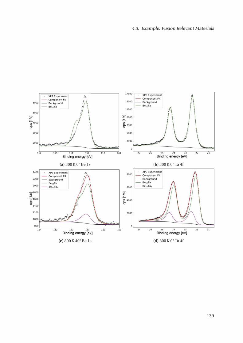
4.3. Example: Fusion Relevant Materials
(a) 300 K 0° Be 1s (b) 300 K 0° Ta 4f
(c) 800 K 40° Be 1s (d) 800 K 0° Ta 4f
139
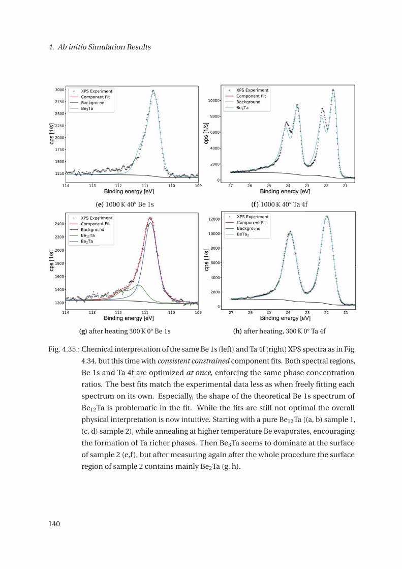
4. Ab initio Simulation Results
(e) 1000 K 40° Be 1s (f ) 1000 K 40° Ta 4f
(g) after heating 300 K 0° Be 1s (h) after heating, 300 K 0° Ta 4f
Fig. 4.35.: Chemical interpretation of the same Be 1s (left) and Ta 4f (right) XPS spectra as in Fig.
4.34, but this time with consistent constrained component fits. Both spectral regions,
Be 1s and Ta 4f are optimized at once, enforcing the same phase concentration
ratios. The best fits match the experimental data less as when freely fitting each
spectrum on its own. Especially, the shape of the theoretical Be 1s spectrum of
Be12Ta is problematic in the fit. While the fits are still not optimal the overall
physical interpretation is now intuitive. Starting with a pure Be12Ta ((a, b) sample 1,
(c, d) sample 2), while annealing at higher temperature Be evaporates, encouraging
the formation of Ta richer phases. Then Be3Ta seems to dominate at the surface
of sample 2 (e,f), but after measuring again after the whole procedure the surface
region of sample 2 contains mainly Be2Ta (g, h).
140

4.3. Example: Fusion Relevant Materials
database symmetry material enthalpy of formation (PBE) volume
identifier group formula [eV/atom] scale V/V0
58738 I 4/mcm 140 BeTa2 -0.170 1.01557
616431 P 4/mbm 127 Be2Ta3 -0.181 1.01627
616428 F d-3mS 227 Be2Ta -0.191 1.00725
616429 R -3mH 166 Be3Ta -0.236 1.01231
616430 R -3mH 166 Be17Ta2 -0.179 0.99092
109317 I 4/mmm 139 Be12Ta -0.138 0.98561
Tab. 4.8.: Ab initio enthalpy of formation for most stable compounds of the Be-Ta system are
listed. From a Birch-Murnaghan equation of states fit the unit-cell volume with the
lowest total energy for the PBE functional is found. The reported volume scales
V/V0 are with respect to the experimental reported volume V0 of the unit cell of the
crystal.
the Be 1s states Voigt profiles were applied as peak-function form while for the 4f states the
asymmetric LA form was used. The asymmetric peak shape introduces one additional degrees
of freedom, which makes the least squares fitting harder, taking more iterations. The same
asymmetry is assumed for all Ta 4f chemical environments within one 4f spectrum.
The experimental Ta 4f splitting was determined to be 1.92 eV [90]. This splitting is ap-
plied in the fitting since the DFT results of 1.98 eV deviates to much from experiment. Other
doublet separations predicted by DFT are also slightly larger like 11.56 eV [90] versus mea-
sured 11.50 eV for the Ta 4ds and for the Ta 4ps 62.96 eV [90] versus the measured 62.50 eV
separation.
Unfortunately, these first concentrations ratios results of Fig. 4.34 and the preferred phases
in the Be 1s fits (left) do not compare well to the phases found in the 4f fits (right). These first
results are problematic, since we believe both spectra to arise from the same sample area and
the same information depth. Furthermore, we also believe that the sample did not change
during the measurement time. In the Be-Ta system Be2Ta and BeTa2 both have only a very
small Ta 4f shift, making the variance of the Ta reference problematic. Also these phases have
large Be 1s shifts and it should be clear from the Be 1s if they are in the information depth or
not.
Fitting first the Be 1s then the Ta 4f with the same phases and constrained concentration
ratios did not resolve the mismatch. To overcome this problem both spectral regions are
fitted within one optimization enforcing the same phase concentration ratios. This leads in
the cases of mixed phases to an additional significant reduction in optimization parameters,
which is good. The same spectra with these consistent component fits are shown in Fig. 4.35.
141

4. Ab initio Simulation Results
material Be 1s Be 1s DFT Ta 4f7/2 Ta 4f DFT
formula electrons CLSs [eV] electrons CLSs [eV]
BeTa2 4 2.128 32 -0.10
Be2Ta3 8 2.170 16,32 0.22, 0.12
Be2Ta 8 1.265 16 0.18
Be3Ta 2,12,4 1.427, 1.368, 0.878 16,8 0.19, -0.45
Be17Ta2 6,12,12,4 0.291, 0.641, 0.755, 0.784 8 -0.92
Be12Ta 8,8,8 0.877, 0.206, 0.767 8 -0.54
Tab. 4.9.: Ab initio results of all core-level shifts of most stable compounds of the Be-Ta system
and how many Be 1s electrons contribute per each unit cell of these systems. De-
pending on the crystal symmetry there are several chemical environments resulting
in different chemical shifts. All these chemical shifts are currently experimentally
not known in the literature. From this data all XPS spectra containing a mixture of
Be-Ti binary phases can be fitted.
These fits match the data not that well overall as the individual fits did before, but now the
phase content is consistent. From this interpretation can be concluded that there is Be12Ta
in both samples. Though the Ta 4f can be explained with mainly the Be12Ta phase, the Be 1s
results for Be12Ta cannot capture the form of the spectrum. The origin of this form is still to
be understood. To gain enough statistics in the Be 1s spectra, it takes hours to measure them.
From the experimental side should be checked if the sample does indeed not change, and no
averaged out process is seen. From the theory side it should be checked if the chemical shifts
for Be12Ta do not change much for the fully relaxed cell within DFT (the ground state PBE
lattice volume was 1.5 % smaller). Also with beyond DFT methods it could be checked if the
form of the Be 1s peak is indeed not asymmetric at all. The influence of a consistent Shirely
background for spectra containing multiple chemical environments should be tested.
After annealing to 1000 K the spectrum clearly changed and the best consistent fit contains
only Be3Ta. This can capture the shift and form of the Be 1s spectrum and the splitting of the
Ta 4f. Though the fit fails to match the 4f data exactly. Some intensity is missing in the higher
binding energy peaks and overestimating their flanks. Be has evaporated from the sample
leaving this stable phase in the transition at the surface.
At higher annealing temperatures or after preferential Ar sputtering mainly the Ta richer
Be2Ta is found at the surface. The Ta 4f spectra can again be very well explained by mainly
coming from the Be2Ta phase, while it is also clearly seen in the Be 1s spectra. Though the
overall form of the Be 1s spectra can again not be very well explained by just Be2Ta.
Comparing the component fit with the traditional fit evaluation of the data by N. Helfer [229]
142

4.3. Example: Fusion Relevant Materials
shows that both can fit the spectra well. The component fit always needs less fit parameters as
is summed up in Tab. 4.10. Fitting both spectra usually reduces the number of fit parameters
again. In the most simple case, a spectrum with a single phase with one contribution, all
approaches need the same amount of fit parameters. The problems with the single spectra
component fit are expected to also arise in the tradition approach. The component fit enforces
a chemical interpretation or leads to a bad or failed fit, which points to missing or wrong
information.
XPS spectrum N Fit parameters N Fit parameters N Fit parameters
Fig. 4.34, 4.35 traditional [229] individual fits Fig. 4.34 both in one fit Fig. 4.35
(a+b) (8+9)=17 (6+6)=12 (4+5)=9
(c+d) (8+9)=17 (6+7)=13 (5+5)=10
(e+f) (8+8)=16 (6+8)=14 (5+5)=10
(g+h) (8+9)=17 (5+5)=10 (5+6)=11
Tab. 4.10.: This table compares the number of fit parameters needed to fit the presented Be-Ta
spectra. The traditional evaluation from [229] using UniFit always requires even for
these quite simple spectra more fit parameters than the component fit. By fitting
the Be 1s and Ta 4f spectra within one optimization enforcing the same phase
content the number of fit parameters (last column) is even further reduced. For
single phase spectra containing one atom-type no reduction in fit parameters is
achievable.
4.3.4. Core-level Shifts of selected other Systems
Materials in nature contain nearly always impurities, and it is cost intensive to purify materials.
Here, further core-level shift (CLS) data on metallic binary alloys from the small material
screening project is listed. Systems containing Be and W might be of further interest for
the fusion community. Be alloys are also used in the aerospace and space flight industries.
Tungsten has also various further applications and is for example mixed into some high-
tech steels. The Be 1s CLS are collected in Tab. 4.11 while the W 4f CLS are listed in Tab.
4.12. The chosen Be reference structure in the screening differed from the one selected in
the detailed investigation. The difference in their Be 1s reference is 211 meV, leading to a
systematic difference. An investigation has shown that these structures are very similar in
their total energy per atom, to be consistent I have recalculated the core-level shifts from
the screening with the high-quality reference used before. For W the difference in the W 4f
references was only 17 meV, which I did not correct for. This demonstrates how the choice
143

4. Ab initio Simulation Results
of the reference structure may introduce systematic biases in the data. This bias could be
investigated and estimated by looking at the difference in the Kohn-Sham core levels for
different elemental structures. Data discussed in detail in the Be-W, Be-Ti and Be-Ta sections
are excluded from the tables. Be rich phases have often several chemical environments while
the most W alloys have only one chemical environment of tungsten. In Tab. 4.13 the 1s
core-level shifts for converged lithium alloys are listed. The agreement in formation energies
with the VASP program was for these compounds also quite good. Li alloys are important for
battery research and are also used in the Tritium breeding blanket of a fusion reactor.
MP Database Symmetry Material Be Be 1s DFT
Identifier Group Formula atoms CLSs [eV]
mp-603 227 Be2Ag 4 -0.29
mp-12761 139 BeAu2 1 -1.5
mp-1220 216 Be5Au 4, 1 -0.49, -1.87
mp-27757 129 Be4B 2, 2, 4 0.11, 0.18, 0.23
mp-1432 225 Be2B 2 1.25
mp-30425 226 Be13Ba 2, 12, 12 0.82, 0.4, 0.41
mp-11280 191 Be12Ti 2, 6, 2, 2 -0.25, 0.91, -0.19, 0.75
mp-30441 166 Be17Nb2 6, 3, 6, 2 0.83, 0.89, 0.75, 0.38
mp-12648 166 Be17Ti2 2, 6, 6, 3 0.59, 0.9, 0.99, 1.13
mp-2544 166 Be17Zr2 12, 2, 3 0.83, 0.54, 0.92
mp-1845 226 Be13Ca 2, 24 0.83, 0.54
mp-457 226 Be13Ce 24, 2 0.68, 1.09
mp-1878 226 Be13Hf 24, 2 0.68, 1.23
mp-976039 226 Be13Lu 2, 24 1.02, 0.6
mp-855 226 Be13Mg 24, 2 0.42, 0.75
mp-337 226 Be13Pu 2, 24 1.08, 0.75
mp-972891 226 ScBe13 2, 24 1.05, 0.65
mp-2080 226 Be13Sr 2, 12, 12 0.82, 0.48, 0.49
mp-1562 226 Be13Th 12, 12, 2 0.56, 0.55, 1.06
mp-1163 226 Be13U 2, 24 1.09, 0.76
mp-865889 226 Be13Yb 2, 24 0.95, 0.61
mp-30445 226 Be13Zr 2, 24 1.23, 0.71
mp-2553 191 Be2Hf 2 1.45
mp-1018057 63 BeHf 2 1.38
mp-13453 63 BePd3 2 0.27
mp-978963 194 BeTi3 2 0.94
144

4.3. Example: Fusion Relevant Materials
mp-1252 191 Be2Zr 2 1.41
mp-983590 221 Be3Fe 3 0.64
mp-973292 221 Be3Mn 3 0.89
mp-977552 221 Be3Tc 3 0.11
mp-2031 227 Be2Cu 2, 2 0.59, 0.6
mp-2028 227 Be2Nb 4 1.14
mp-11272 127 Be2Nb3 4 1.94
mp-2676 227 Be2Ta 4 1.2
mp-1025010 216 Be5Fe 4, 1 1.38, 0.07
mp-2025 191 Be5Hf 2, 3 0.83, 1.11
mp-650 216 Be5Pd 4, 1 0.51, -0.83
mp-11277 191 ScBe5 3, 2 1.05, 0.74
mp-11283 191 Be5Zr 2, 3 0.88, 1.18
mp-984315 194 Be3Ni 2, 4 0.44, 0.43
mp-864894 194 Be3Rh 6 0.14
mp-984612 194 Be3Ru 6 0.39
mp-30438 194 Be2Cr 2, 6 1.57, 1.68
mp-2225 194 Be2Fe 2, 6 1.08, 1.25
mp-11270 194 Be2Mn 6, 2 1.48, 1.36
mp-1677 194 Be2Mo 6, 2 1.19, 1.11
mp-11275 194 Be2Re 6, 2 0.51, 0.4
mp-11281 194 Be2V 2, 6 1.66, 1.72
mp-11282 194 Be2W 6, 2 1.16, 1.04
mp-2323 221 BeCu 1 -0.2
mp-1033 221 BeNi 1 0.37
mp-11274 221 BePd 1 -0.76
mp-13452 139 BePd2 1 -0.13
mp-11276 221 BeRh 1 0.73
mp-11279 221 BeTi 1 0.9
Tab. 4.11.: Core-level shifts collection of other binary compounds from the screening con-
taining Be. Beryllium rich systems have often several Be atom-types per unit cell.
Different atom-types having the same core-level shifts are added together. These
shift are calculated with the same reference structure as for the in detail Be-Ti,
Be-Ta, Be-W evaluation
145

4. Ab initio Simulation Results
MP Database Symmetry Material W W 4f7/2 DFT
Identifier Group Formula atoms CLSs [eV]
mp-30337 182 Al5W 2 0.43
mp-12524 181 Al2W 3 0.74
mp-11696 12 As3W2 2, 2 -0.03, -0.13
mp-1008487 63 BW 2 -0.59
mp-1113 140 BW2 4 -0.07
mp-7832 141 BW 4 -0.6
mp-569803 194 B2W 4 -0.53
mp-11282 194 Be2W 4 0.68
mp-684602 58 CW2 4 0.32
mp-567397 162 CW2 6 0.4
mp-2034 60 CW2 8 0.41
mp-1894 187 CW 1 0.43
mp-23269 148 WCl3 6 -1.4
mp-1008274 221 Co3W 1 -0.43
mp-2157 194 Co3W 2 -0.26
mp-20868 194 Fe2W 4 -0.02
mp-542595 139 Ge2W 1 -0.08
mp-1007761 194 HW 2 0.36
mp-1400 227 HfW2 4 0.6
mp-30744 51 IrW 2 0.1
mp-30745 194 Ir3W 2 -0.88
mp-19066 65 O8W3 2, 1 -0.06, -0.22
mp-11329 12 P2W 2 -0.19
mp-11328 36 P2W 2 -0.09
mp-2420 62 PW 4 -0.42
mp-1018129 71 Pt2W 1 -0.63
mp-30866 194 Rh3W 2 -0.78
mp-862655 194 Ru3W 2 0.12
mp-1620 139 Si2W 1 0.16
mp-31219 140 Si3W5 2, 4, 4 -0.25, -0.39, -0.38
mp-979289 225 W3Ta 1, 2 0.19, 0.4
mp-22693 31 Te2W 4 -0.21
mp-675 227 W2Zr 4 0.58
146
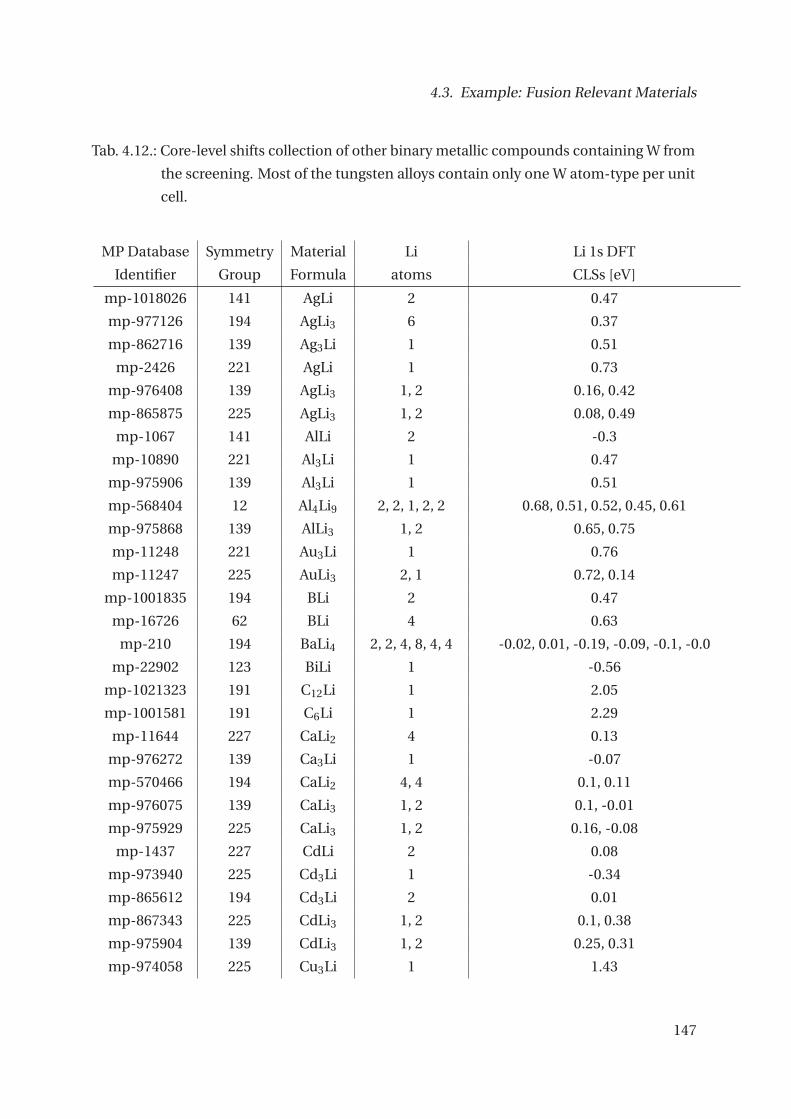
4.3. Example: Fusion Relevant Materials
Tab. 4.12.: Core-level shifts collection of other binary metallic compounds containing W from
the screening. Most of the tungsten alloys contain only one W atom-type per unit
cell.
MP Database Symmetry Material Li Li 1s DFT
Identifier Group Formula atoms CLSs [eV]
mp-1018026 141 AgLi 2 0.47
mp-977126 194 AgLi3 6 0.37
mp-862716 139 Ag3Li 1 0.51
mp-2426 221 AgLi 1 0.73
mp-976408 139 AgLi3 1, 2 0.16, 0.42
mp-865875 225 AgLi3 1, 2 0.08, 0.49
mp-1067 141 AlLi 2 -0.3
mp-10890 221 Al3Li 1 0.47
mp-975906 139 Al3Li 1 0.51
mp-568404 12 Al4Li9 2, 2, 1, 2, 2 0.68, 0.51, 0.52, 0.45, 0.61
mp-975868 139 AlLi3 1, 2 0.65, 0.75
mp-11248 221 Au3Li 1 0.76
mp-11247 225 AuLi3 2, 1 0.72, 0.14
mp-1001835 194 BLi 2 0.47
mp-16726 62 BLi 4 0.63
mp-210 194 BaLi4 2, 2, 4, 8, 4, 4 -0.02, 0.01, -0.19, -0.09, -0.1, -0.0
mp-22902 123 BiLi 1 -0.56
mp-1021323 191 C12Li 1 2.05
mp-1001581 191 C6Li 1 2.29
mp-11644 227 CaLi2 4 0.13
mp-976272 139 Ca3Li 1 -0.07
mp-570466 194 CaLi2 4, 4 0.1, 0.11
mp-976075 139 CaLi3 1, 2 0.1, -0.01
mp-975929 225 CaLi3 1, 2 0.16, -0.08
mp-1437 227 CdLi 2 0.08
mp-973940 225 Cd3Li 1 -0.34
mp-865612 194 Cd3Li 2 0.01
mp-867343 225 CdLi3 1, 2 0.1, 0.38
mp-975904 139 CdLi3 1, 2 0.25, 0.31
mp-974058 225 Cu3Li 1 1.43
147

4. Ab initio Simulation Results
mp-862658 139 Cu3Li 1 1.4
mp-975882 139 CuLi3 2, 1 0.63, 0.55
mp-567306 166 Ga7Li3 6 -0.8
mp-1307 227 GaLi 2 -0.74
mp-29210 63 GaLi2 2, 2 0.46, 0.71
mp-867205 221 Ga3Li 1 0.11
mp-976025 139 GaLi3 1, 2 0.54, 0.67
mp-976023 225 GaLi3 2, 1 0.88, 0.45
mp-29631 63 Ge6Li11 4, 2, 2, 4, 2, 4, 4 0.72, 0.5, 0.21, 0.61, 0.79, 0.52, 0.57
mp-29630 65 Ge2Li7 5, 4, 1, 4 0.52, 0.31, -0.35, 0.56
mp-8490 141 GeLi 4, 2 0.1, 0.3
mp-9918 88 GeLi 8 -0.12
mp-973824 225 Hg3Li 1 -0.74
mp-2012 221 HgLi 1 0.12
mp-1646 225 HgLi3 2, 1 0.44, 0.04
mp-976047 139 HgLi3 2, 1 0.34, 0.19
mp-22460 227 InLi 2 -0.99
mp-31324 63 InLi2 2, 2 0.16, 0.39
mp-973748 139 In3Li 1 -0.4
mp-867226 225 InLi3 1, 2 0.27, 0.6
mp-976055 139 InLi3 1, 2 0.27, 0.43
mp-30738 44 Ir3Li 1 1.86
mp-9563 190 SbLi2 6, 6 0.03, 0.27
mp-30769 164 Sn5Li13 2, 1, 2, 2, 4, 2 -0.02, -0.13, 0.37, 0.58, 0.19, 0.56
mp-30767 65 Sn2Li7 4, 1, 4, 1, 4 0.37, 0.25, 0.2, -0.3, 0.38
mp-30768 11 Sn3Li7 2, 2, 2, 2, 2, 2, 2 -0.04, -0.03, 0.33, -0.19, -0.23, 0.23, 0.41
mp-672287 55 Si4Li13 2, 4, 4, 4, 4, 4, 4 0.9, 0.66, 0.62, 0.81, 0.99, 0.75, 0.85
mp-973374 63 Mg2Li 2 0.28
mp-973455 2 Mg2Li 2 0.35
mp-1018789 58 O2Li 2 4.05
mp-728 191 PdLi2 2 0.78
mp-2170 191 PtLi2 2 0.9
mp-30764 227 Pt2Li 2 0.76
mp-975799 194 Zn3Li 2 0.65
mp-976139 25 MgLi3 2, 1 0.29, 0.12
mp-976254 221 MgLi3 3 0.33
148

4.3. Example: Fusion Relevant Materials
mp-976256 225 MgLi3 2, 1 0.29, 0.22
mp-976244 8 MgLi 1, 1, 1 0.37, 0.36, 0.31
mp-976262 8 MgLi 2, 1 0.36, 0.35
mp-976239 38 MgLi 1, 1, 1 0.44, 0.4, 0.39
mp-30760 139 PbLi3 1, 2 0.01, 0.5
mp-976281 139 PdLi3 2, 1 0.83, 0.66
mp-11489 225 PdLi3 1, 2 0.45, 1.05
mp-976322 139 PtLi3 1, 2 0.89, 1.18
mp-7396 225 TlLi3 2, 1 0.44, 0.09
mp-976412 225 ZnLi3 1, 2 0.24, 0.58
mp-976414 139 ZnLi3 2, 1 0.51, 0.44
mp-977207 194 MgLi2 4 0.17
mp-976885 155 MgLi2 1, 3 0.2, 0.12
mp-976843 12 MgLi2 2, 2 0.15, 0.26
mp-976982 63 MgLi2 2, 2 0.11, 0.31
mp-982380 8 MgLi2 1, 1, 1, 1 0.1, 0.14, 0.21, 0.22
mp-7924 127 Sn5Li2 4 -0.17
mp-977122 38 MgLi5 1, 1, 1, 1, 1 0.16, 0.27, 0.06, 0.18, 0.12
mp-976944 8 MgLi5 1, 1, 1, 2 0.17, 0.09, 0.2, 0.21
mp-865604 189 MgLi5 3, 2 0.17, 0.28
mp-973316 194 NaLi3 6 -0.34
mp-13444 141 SnLi 4, 2 -0.32, -0.21
mp-30761 164 Pb2Li7 2, 2, 1, 2 0.24, 0.28, -0.21, 0.41
mp-27587 12 Pb3Li8 2, 2, 4 0.02, -0.18, 0.31
mp-795 88 SiLi 8 0.22
mp-7507 136 Sr3Li2 8 -0.17
mp-865939 12 Mg2Li 1 0.38
mp-2744 187 PdLi 1 0.96
mp-861931 221 Pt3Li 1 1.67
mp-600561 187 RhLi 1 1.38
mp-1001787 44 Rh3Li 1 1.98
mp-865907 225 Zn3Li 1 0.36
Tab. 4.13.: Core-level shifts collection of other binary metallic compounds containing Li from
the screening. Many of the lithium alloys contain several Li atom-types per unit
cell. The crystal structures were extracted from the materials Project (MP).
149

4. Ab initio Simulation Results
4.4. Ab initio Simulation Results Sum-up
It was demonstrated that material screening with the all-electron FLAPW method, especially
with the FLEUR code is possible. The challenging part is the automatic choice of FLAPW
parameters and electronic setup which is robust while describing the given system right and
still allowing for accurate comparisons of total energies between materials. Furthermore, it
was demonstrated that the default FLAPW parameters of FLEUR are not always ready for this
challenge and point to possible ways of improvement, like better determination of muffin-tin
radii and further flexibility in the basis cutoffs for good matching criteria. For my rather
small proof of principle high-throughput project I have fixed the FLAPW parameters for each
element. Similar things were done in past works like for the full-potential linear muffin-tin
orbital (FP-LMTO) calculations of the Electronic Structure Project (ESP) [58, 312]. The usual
run mode of the exciting FLAPW code [313, 314] uses fixed species parameters stored in files.
Workflows from the AiiDA-FLEUR package have been deployed to calculate the initial-
state core-level shifts of known binary metals (4435 out of 5058) from the Materials Project.
For elemental references the elemental structures (1271) of the ICSD have been calculated.
This small proof of concept one shot project ran for two weeks totaling over 9000 FLEUR
simulations with different resource requirements managed by AiiDA. The overall success
rate was 68.6 % achieved with the SCF-workflow. Overall, 7.1 % failed for various reasons,
24.3 % did not reach convergence. This is to be seen as a snapshot in time. Most of the non-
converged systems were f elements which were calculated with collinear magnetism and spin
orbit coupling. All systems were calculated with spin orbit coupling included. The actually
overall success rate of non f-systems was lowered by a hybrid parallelization specification
mistake which lead to long run times. So not only the fidelity of the FLEUR code but also the
workflow has to improved. Certain easy user mistakes are to be avoided.
For evaluating the quality of the produced data differences and agreements of FLEUR
and VASP results were pointed out for formation enthalpies and the calculated bandgap. A
comparison of chemical shifts with the overlap of 133 entries of the NIST XPS database [90]
showed partially agreement but a large spread in the experimental data. Without any quality
measures in place, chemical shift results from this run can include systematic uncertainties
due to the reference structure choice. To benchmark the chemical shifts in the database it is
better to apply them in the evaluation of single crystal XPS spectra.
Results for the Be-W, Be-Ti, Be-Ta systems were presented in more detail including convex-
hull constructions and equation of states. From the calculated core-level shifts and atom-type
information theoretical predicted single-phase spectra were constructed. With these theo-
retical spectra experimental XPS spectra measured by colleagues were fitted and chemically
interpreted. The developed component fit method was compared to traditional fit procedure.
150

4.4. Ab initio Simulation Results Sum-up
The Be 1s spectra were fitted with Voigt profile peak shapes for each chemical environment
while for the 4f spectra asymmetric peak shapes were necessary. The resulting concentrations
from the phases in the Be 1s fits did not correspond well to the best fit of the 4f spectra. This
can be overcome by fitting both spectra at once, constraining the phase content.
It becomes clear from these XPS spectra evaluations, that the component fit approach
provides new opportunities, but relies on very precise data and experiments. The method
should be further benchmarked against high-resolution single crystal spectra with known
broadenings and accurately known elemental reference to check the DFT result very precisely.
Also the asymmetric LA shape is not optimal, since changing the gaussian broadening does
not affect the asymmetry and to increase the tail significantly the Lorentzian broadening has
also to become quite large. Additionally trying out other optimizers, besides least squares with
gradient-decent, may improve the method, since there may be local minima, dependencies on
the starting points and bounds to be dealt with. Also investigation surface effects and surface
core-level shifts might complete the picture. The approximation of the spectral background
needs to be included consistently in the fit an revised for several chemical environments. The
standard background assume one contribution within one main peak which may introduce
systematic errors in the background.
151


5. Conclusion and Outlook
Designing and optimizing materials on the computer is a profound challenge to accelerate
and bring down the cost of innovation driven by materials. In condensed matter physics,
materials science and chemistry computational methods and tools play an ever growing role
when calculating properties of materials. The same is true for designing and predicting new
ideal (nano) materials. Ab initio methods provide practical computable approximations to
the many-body problem of many electrons. Density functional theory is a widely applied ab
initio method to calculate observables as a functional of the electron density. Through a mini-
mization principle the ground state density of a many-body system can be self-consistently
determined by solving an auxiliary Kohn-Sham system. Data from ab initio simulations
is valuable for many applications and data hubs emerged in the community out of larger
projects. However all-electron reference data is rare, most of the data (≈ 90%) available comes
from pseudo-potential plane wave methods.
Chemical configuration space is too large to just screen through it by brute force. Practical
methods are needed to cope with its size beyond high-throughput computing and automation
of tasks. These methods need to determine what configurations are worth calculating in detail,
or may yield promising properties. We have demonstrated that with the AiiDA framework
high-throughput calculations of around one million calculation tasks per week are possible.
In this thesis the open source AiiDA-FLEUR package was developed, which allows for au-
tomation of calculations with the all-electron quantum engine FLEUR. The FLEUR program
as well as many other electronic structure packages can now be deployed together within a
single high-level python work environment using AiiDA, allowing to profit from the individual
strengths of each package. Workflows are physical property calculator protocols for a given
task or sub task. Expert knowledge and strategies can be embedded into workflows allowing
for robustness, fault tolerance and fidelity. Within this work workflows to converge a FLEUR
calculation, to calculate an equation of states, a density of states, a band structure, forma-
tion energies, core-level shifts and binding energies have been implemented. Some of these
workflows were deployed on larger (O (100)−O (1000)) sets of crystal structures from various
153

5. Conclusion and Outlook
sources.
X-ray photoemission spectroscopy is a powerful tool to gain insight into the chemical com-
position within the surface region of a sample. It is widely applied in research and industry
for material characterization. The exact analysis of high resolution XPS spectra is still an
ongoing challenge which poses various difficulties. Core-level shifts provide insight on the
chemical environments and are a key component for such analysis. It was argued that a
usual fitting approach with only few constraints has fundamental problems with samples
containing phases which have multiple not clearly separated chemical environments of the
same element. Therefore, the application range of the usual approach is rather limited to
simple phases and their simple mixtures. Since some important spectral properties of XPS
spectra can be computed via ab initio methods, a physically motivated fit built on ab initio
data was proposed. This data-driven evaluation approach often contains less degrees of
freedom and has the potential to scale to complexer systems. Also this evaluation strategy
allows to build in additional constraints like an experimentally known stoichiometry or to fit
several spectra with the same phase content at once. This way additional degrees of freedom
can be eliminated from the fitting. Furthermore, linear dependencies between the phases
can be determined and the method allows for the extraction of phase concentrations.
A proof of principle application of this data-driven component-fit approach was demon-
strated on ’well behaved’ high-resolution XPS spectra of main core-level lines of Be-W, Be-Ti
and Be-Ta systems. ’Well behaved’ meaning without many other physical effects having major
contributions to these spectra. The Be-Ti and Be-Ta data was measured at the IEK-4 by Nicola
Helfer. These material systems are of interest to the nuclear fusion community. The alloying
under certain annealing temperatures could be better understood with this developed analy-
sis, which was not possible to this extent beforehand. The best fit for individual core-level
spectra might not be consistent with the best fit results of other core-level lines. Fitting several
different core-level spectra of the same sample at once enforces consistency, or may point to
sources of inconsistency.
Furthermore, in a small proof of principle screening project with FLEUR the initial-state
core-level shifts were calculated for 4435 binary metals, out of 5058 stable materials found in
the Materials Project. By enabling this project and from executing it, we have learned about
the robustness of the FLEUR program, data infrastructure and throughput capabilities of
computing resources. From this knowledge future high-throughput projects with FLEUR
may profit. In this project we have calculated more than twice as many main-line core-level
154

shifts than are found in the NIST XPS database, a mature experimental numerical reference
database, which is representative for the whole literature. Our data set allows for evaluation of
XPS spectra of these metals. The overlap from the materials with the NIST database was only
133 core lines of 45 materials. The comparison of data posed challenges due a wide spread
in the NIST data and no in detail uncertainty investigation of our data. Some properties
from the binary materials were also quantitatively compared to VASP simulations from the
Materials Project. As elemental references the energetically favorable structures from the
ICSD were taken. A wrong reference will lead to systematic differences in the core-level shifts
and formation energies of systems containing that element. Elements with open 4f and 5f
shells still pose a challenge to the SCF workflow as they would need special treatment within
DFT.
As an outlook, in the future the tools for computational material design developed in our
community and ab initio packages become more robust and will bring us closer towards
driving materials discovery and materials optimization. Also all-electron programs will enter
the high-throughput highway. Individual groups and projects will contribute to curated and
searchable data repositories. Larger comparisons and accuracy classification of DFT quantum
engines will become feasible. On the way the robustness and scalability of quantum engines
and frameworks will improve. Bringing the code packages to a high-level platform will allow
to harvest their individual strengths bringing us closer to a materials design infrastructure,
saving resources by not redoing things over and over again. Meta workflows which are ab initio
package agnostic might emerge from community efforts. Online platforms or companies
can provide utilities and services with a higher visibility to serve outside communities and
industry.
For theFLEURprogram additional workflows with high-throughput capabilities implement-
ing advanced features will emerge. The current basic workflows and utilities of AiiDA-FLEUR
will be reused and refined in these tasks. Workflows and tools from also other ab initio
packages may become helpful for calculating other important properties of fusion relevant
materials, like diffusion properties of materials, thermal conductivity, influence of crystal
defects, mechanical properties, or oxidization properties. This may help in the research of
finding and characterizing promising materials or their sub components and precipitates.
With a structural symmetry analysis one could check which entries in the NIST database
should be seen rather carefully, by checking if the crystal structures of the reported materials
in NIST have several atom-types and therefore may give rise to several different core-level
155

5. Conclusion and Outlook
shifts.
Through ab initio methods a database including all relevant properties of core-level spectra
of all known materials and surfaces may be created, forming the foundation for data-driven
spectra interpretation. With machine learning this base data may be extrapolated to arbitrary
system sizes or collective surface contributions. On top of such data an evaluation program
like casaXPS or UniFit deploying advanced smart component-fits may solve large parts of the
XPS spectra interpretation problem. Such a tool or service may accelerate materials discovery,
material characterization and innovation in industries and laboratories around the world.
156

Appendices
157

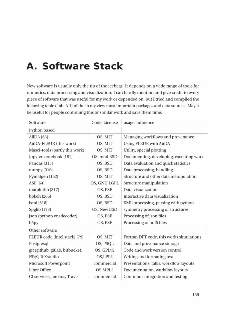
A. Software Stack
New software is usually only the tip of the iceberg. It depends on a wide range of tools for
numerics, data processing and visualization. I can hardly mention and give credit to every
piece of software that was useful for my work or depended on, but I tried and compiled the
following table (Tab. A.1) of the in my view most important packages and data sources. May it
be useful for people continuing this or similar work and save them time.
Software Code, License usage, influence
Python based
AiiDA [63] OS, MIT Managing workflows and provenance
AiiDA-FLEUR (this work) OS, MIT Using FLEUR with AiiDA
Masci-tools (partly this work) OS, MIT Utility, special plotting
Jupyter-notebook [181] OS, mod BSD Documenting, developing, executing work
Pandas [315] OS, BSD Data evaluation and quick statistics
numpy [316] OS, BSD Data processing, handling
Pymatgen [152] OS, MIT Structure and other data manipulation
ASE [64] OS, GNU LGPL Structure manipulation
matplotlib [317] OS, PSF Data visualization
bokeh [266] OS, BSD Interactive data visualization
lxml [318] OS, BSD XML processing, parsing with python
Spglib [178] OS, New BSD symmetry processing of structures
json (python en/decoder) OS, PSF Processing of json files
h5py OS, PSF Processing of hdf5 files
Other software
FLEUR code (intel stack) [79] OS, MIT Fortran DFT code, this works simulations
Postgresql OS, PSQL Data and provenance storage
git (github, gitlab, bitbucket) OS, GPLv2 Code and work version control
LATEX, TeXstudio OS,LPPL Writing and formating text
Microsoft Powerpoint commercial Presentations, talks, workflow layouts
Libre Office OS,MPL2 Documentation, workflow layouts
CI services, Jenkins, Travis commercial Continous integration and testing
159

A. Software Stack
sphinx [174] OS, Sphinx Code documentation
read the docs [175] OS, MIT Hosting code documentation
Graphviz [319–321] OS, GPL v1.0 Database small graph visualizations
Gephi [322] OS, GPL Database large graph visualizations
docker, docker-compose [323] commercial AiiDA-FLEUR tutorial and tests
dbbeaver [324] OS, ASL Database status, management and changes
postgres app mac [325] OS, PSQL PostgreSQL deployment on mac
postico app mac [326] commercial Database changes on mac
pgadmin [327] OS, PSQL Database status and management
gource [328] OS,GPL3 Repository visualization
Databases
ICSD [89] commercial Structure data source for this work
Materials Project, API [39, 54] open data login needed, structure data source
AFLOWLib [56] open data Structure data source for this work
OQMD and its API [55] open data Structure data source (mysql db)
NIST XPS [90] open data Database of XPS binding energies
Materialscloud [59] open data Visualization of data, and data source
COD [134] open data Structure data source for this work
Tab. A.1.: Notice: Dependencies of the software packages are not mentioned, only if they
have been used extensively as stand alone. Each category is roughly sorted after
relevance, with most relevant first. Default software from the Linux and Mac OS
infrastructure of the PGI and computing resources are also not mentioned.
160
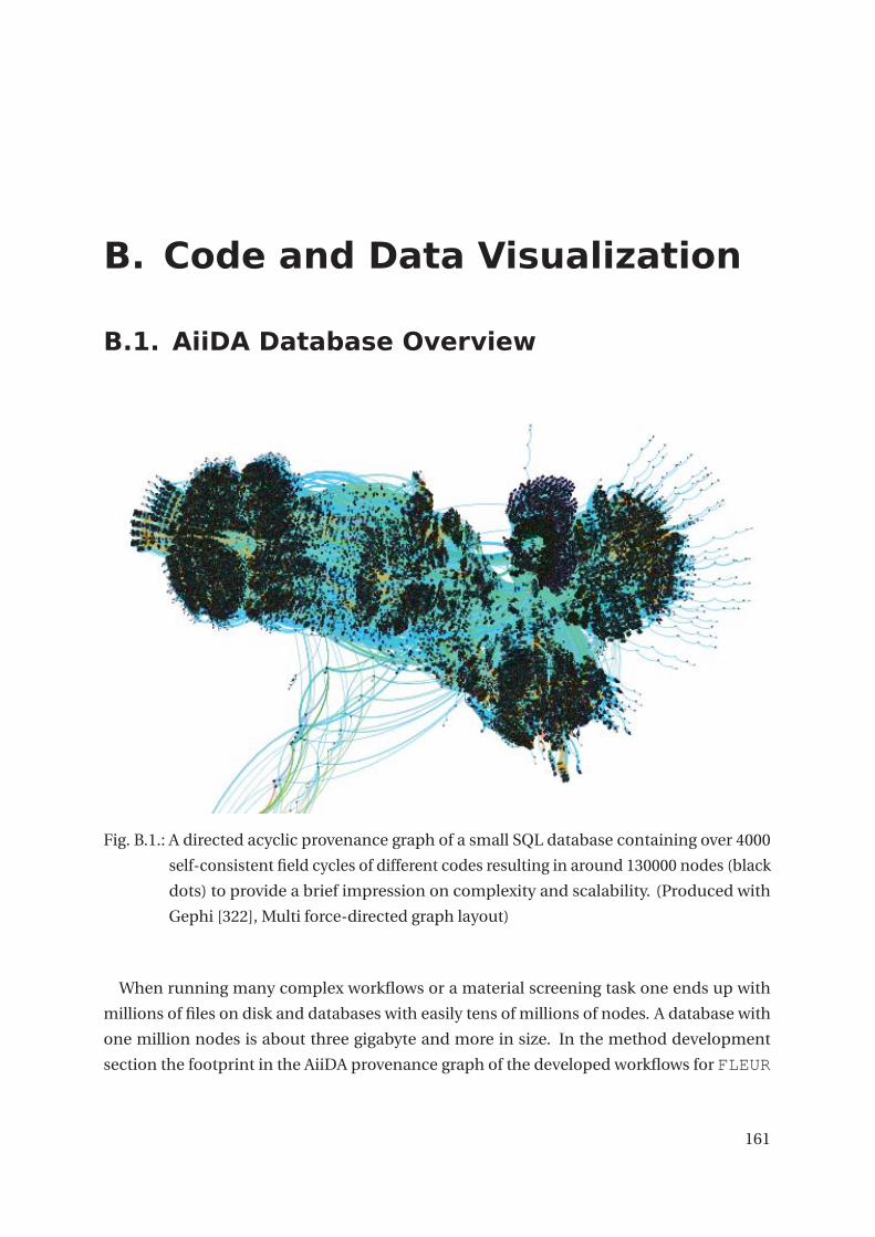
B. Code and Data Visualization
B.1. AiiDA Database Overview
Fig. B.1.: A directed acyclic provenance graph of a small SQL database containing over 4000
self-consistent field cycles of different codes resulting in around 130000 nodes (black
dots) to provide a brief impression on complexity and scalability. (Produced with
Gephi [322], Multi force-directed graph layout)
When running many complex workflows or a material screening task one ends up with
millions of files on disk and databases with easily tens of millions of nodes. A database with
one million nodes is about three gigabyte and more in size. In the method development
section the footprint in the AiiDA provenance graph of the developed workflows for FLEUR
161

B. Code and Data Visualization
were discussed. To get an impression about the complexity of a rather small overall, cumu-
lative AiiDA provenance graph containing some workflows with different codes on various
computers is shown in Fig. B.1. The graph depicts about 4000 self-consistent field workflows
with different codes, versions and computing resources, resulting in about 130,000 nodes
(black dots). The graph is layouted with a parallel multi-force-atlas graph-layout algorithm
using Gephi [322]. Clusters of nodes evolve around different highly connected FLEUR code
nodes on diverse computing resources. Crystallographic Information File (CIF) data nodes
from which crystal structures have been extracted dangle loosely connected around the edges.
Such a plain full graph visualization is for the extraction of physics or browsing interactively
through the data rather not useful. Force graph visualization might be in general helpful to
visualize structure property maps, or other higher dimentional complex relationships.
Node type quantity relative content comment
ParameterData 221670 38.68 % should be less, AiiDA bug
WorkCalculation 147718 25.77 % should be less, AiiDA bug
StructureData 38259 6.68 %
RemoteData 34500 6.02 % FLEUR plus inpgen
FolderData 34202 5.96 % FLEUR plus inpgen
CifData 32232 5.62 %
FleurinpData 29202 5.10 % get modified in workflows
FleurinputgenCalculation 17701 3.09 %
FleurCalculation 17015 2.97 %
Others 600 0.10 %
Tab. B.1.: Snapshot of the node content of the database with after the first metal screening
results. The (provenance) and input preparation overhead is 33 nodes per FLEUR
calculation. This overhead depends in detail on the workflows deployed and their
design. Under high-throughput conditions, sometimes the tasks of small fast Work-
Calculations within workflows were executed multiple times (100-1000) for some
reason (bug in AiiDA). This causes an excess of WorkCalculations and Parameter-
Data nodes. The real overhead is probably more around 10-15 nodes. This bug
might be fixed in newer AiiDA versions. These double nodes may be cleaned from
the database. Also in newer AiiDA and AiiDA-FLEUR version most of the WorkCal-
culation block will largely consist out of CalcFunctions.
162

B.2. Disk footprint Overview
B.2. Disk footprint Overview
Fig. B.2 displays a birds-eye view on disk usage of a small AiiDA workstation. While the
Postgres databases creates files with a certain maximum fixed size, in this case one GB the
repository has a lot of files with different sizes. In this case all files are quite small. For FLEUR
the largest files are the ’out.xml’ files and the ’last_cdn.hdf’ files, which are for small systems
only up to 100 MB. This view should point out the requirements on storage of the database and
the repository. When replacing the repository with an object store the AiiDA repository would
be one large file, or several smaller files of fixed size as in the database case. Visualization of
the screenings data footprint would have taken long and would add nothing special to the
picture.
Fig. B.2.: Bird-eye view of disk usage of a small AiiDA workstation (120 GB). The AiiDA reposi-
tory with many small files is shown on the left. The larger boxes correspond to the
charge density files of the last iteration and ’out.xml’ files. The disk footprint of
the PostgreSQL databases (on the right) are several larger files with around 1 GB in
size. This points out the different storage requirements for the repository and the
database. Lastest database backups files and files with additional parsed informa-
tion for evaluation can also become quite large. Most of the rest is data unrelated to
AiiDA, or other small environments. (created with GrandPerspective.app [329])
163

B. Code and Data Visualization
B.3. Repository Code Overview
Software is not static. During the development (2016-2018) of AiiDA-FLEUR and masci-tools
also AiiDA and the FLEUR program changed significantly. The progress of the source code
from the software packages over time is visualized in the following figures to give credit to the
developer teams and to provide insight into these ecosystems. The figures have been created
from the git history of the packages. Fig. B.3 shows the code development of the FLEUR team
including all files. Prior to 2016 the code was not openly available within a git repository.
The initial commit of the full previous code in Q2 2016 is cut off in the graph. In Fig. B.4 the
progress of the python code of the aiida-core package is shown. The masci-tools repository
python code development shown in Fig. B.6, it contains utility which is independent of AiiDA
and can be reused within the institute. It is a mixed code package. Fig. B.6 documents the
status of solely the python code in the AiiDA-FLEUR package. Contributions to AiiDA-FLEUR
from Vasily Tseplyaev started in the fourth quarter of 2018. Before 2017 the package was in
another repository under a different name, which history is not included.
Fig. B.3.: The gitlab repository of FLEURwas created in the second quarter of 2016. The graph
shows the total changes and activity on all files. The large initial commit of previous
code of FLEUR in Q2 2016 is cut off. The total lines refer to all file types.
164

B.3. Repository Code Overview
Fig. B.4.: AiiDA-core package development over time is visualized in this graph. The total lines
refer to python code files only.
Fig. B.5.: The evolution of the Masci-tools repository, containing AiiDA independent utility
and tools applied at the IAS-1 and rather specific to electronic structure.
165

B. Code and Data Visualization
Fig. B.6.: The AiiDA-FLEUR development started at the end of 2015, but the repository was
renamed and moved, which is why the history is only visible since Q2 2016 with a
large initial changes. The total lines refer to python code files only.
166

Conventions and Abbreviations
In this work, we stick to the following conventions in mathematical expressions:
Symbol Explanation
r bold 3 or 4-dimensional vector
r bold hat normalized 3-dimensional vector
c underline general vector
M double underline general matrix
The following abbreviations and physical constants are used:
Abbr. Meaning
AI Artificial Intelligence
API Application Programming Interface
a0 Bohr radius
bcc body-centered cubic
BE binding energy
BZ Brillouin zone
CLS core-level shift
CPU central processing unit
cps counts per sweep
DB data base
DFT density functional theory
DOS density of states
EOS equation of states
ESCA electron spectroscopy for chemical analysis
Conventions and Abbreviations
fcc face-centered cubic
FWHM full-width half-maximum
FLAPW full-potential linearized augmented-plane-wave (method)
FLOPS floating point operations per second
FP full potential
GF Green function
GGA general gradient approximation
hcp hexagonal close-packed
HDD hard disk drive
HPC high-performance computing
HTC high-throughput computing
HTML Hypertext Markup Language
IAS Institute of Advanced Simulation
IBZ irreducible Brillouin zone
IEK Institute of Energy and Climate Research
IO input/output
IR interstitial region
ISS ion scattering spectroscopy
IT information technology
ITER International Thermonuclear Experimental Reactor
LA asymmetric Lorentz profile
LDA local density approximation
LO local orbital
MPI Message Passing Interface
MT Muffin tin
MTC Many-tasks computing
NRA Nuclear reaction analysis
OS open source
PBE PBE exchange-correlation (functional)
PCA Principle Component Analysis
PES photoemission spectroscopy
PGI Peter Grünberg Institute
QMA Quantum Merlin Arthur complexity class
RAM random access memory
RBS Rutherford backscattering spectrometry
RMT Muffin-tin radius
168

Conventions and Abbreviations
SCF self-consistent field
SOC spin-orbit coupling
SSD solid state drive
SQL structured query language
UHV ultra-high vacuum
UPS ultraviolet photoelectron spectroscopy
XAS X-ray absorption spectroscopy
XC exchange-correlation (functional)
XML Extensible Markup Language
XRD X-ray diffraction
XPS X-ray photoelectron spectroscopy
169


List of Figures
1.1. Example of a computational supported materials design process. . . . . . . . . 2
2.1. Self-consistency cycle scheme for solving the Kohn-Sham equations. . . . . . . 13
2.2. Visulatization of the Muffin-tin model. . . . . . . . . . . . . . . . . . . . . . . . . 18
2.3. Growth of materials space and databases in material science. . . . . . . . . . . . 21
2.4. The ADES Model in Material Science. . . . . . . . . . . . . . . . . . . . . . . . . . 29
2.5. Layout of the AiiDA framework. . . . . . . . . . . . . . . . . . . . . . . . . . . . . . 29
2.6. Data provenance explained on a simple AiiDA graph. . . . . . . . . . . . . . . . . 30
2.7. Energy level alignment in Photoemission spectroscopy. . . . . . . . . . . . . . . 35
2.8. Schematic view of the photoemission process. . . . . . . . . . . . . . . . . . . . . 37
2.9. XPS experiment setup and apparatus. . . . . . . . . . . . . . . . . . . . . . . . . . 40
2.10.Conventional fitting example of an XPS spectrum. . . . . . . . . . . . . . . . . . 43
2.11.State of the art interpreted XPS spectrum of a mixed Fe-O system. . . . . . . . . 44
3.1. Database node graph of the FLEUR input-generator. . . . . . . . . . . . . . . . . 51
3.2. Database node graph of the FLEUR plug-in. . . . . . . . . . . . . . . . . . . . . . 51
3.3. Flowchart of the FLEUR self-consistent field workflow (SCF). . . . . . . . . . . . 57
3.4. Visualizations with plot_fleur for the SCF workflow. . . . . . . . . . . . . . . . . . 62
3.5. Flowchart and provenance graph of the FLEUR DOS and band structure work-
flows. . . . . . . . . . . . . . . . . . . . . . . . . . . . . . . . . . . . . . . . . . . . . 64
3.6. Visualizations with plot_fleur for the DOS and band structure workflows. . . . . 64
3.7. Flowchart of the equation of state workflow. . . . . . . . . . . . . . . . . . . . . . 65
3.8. Equation of state workflow provenance graph in the database. . . . . . . . . . . 66
3.9. Visualizations with plot_fleur for the equation of states workflow. . . . . . . . . 68
3.10.Layouts of the initial-state core-level shift workflow and the core-hole workflow. 69
3.11.Initial-state core-level shift workflow database graph. . . . . . . . . . . . . . . . 71
3.12.Provenance graph in the database for a core-hole workflow. . . . . . . . . . . . . 76
3.13.Jupyter-notebook app to search through core-hole spectra data. . . . . . . . . . 77
3.14.Jupyter-notebook app to visualize core-hole spectra data. . . . . . . . . . . . . . 78
3.15.Number of symmetry atom-types of binary structures from the ICSD. . . . . . . 80
I
List of Figures
4.1. Element and space group content of crystal structures in the OQMD. . . . . . . 86
4.2. Default FLAPW parameter results by inpgen for crystal structures in the OQMD. 87
4.3. Periodic table visualization of the default muffin-tin radii of OQMD structures. 89
4.4. Default basis cutoff parameters of inpgen for materials in the OQMD. . . . . . 90
4.5. Default k-points and matching criterion by inpgen for OQMD structures. . . . 90
4.6. Default muffin-tin grid parameter by inpgen for OQMD structures. . . . . . . 91
4.7. Matrix visualization of stable binary metals in the Materials Project. . . . . . . . 94
4.8. Periodic table visualization of muffin-tin radii and electronic configuration for
the screening of binary metals. . . . . . . . . . . . . . . . . . . . . . . . . . . . . . 96
4.9. Distributions of FLAPW basis cutoff parameters from the binary metal screening. 97
4.10.Distributions of K-point densities and matching criterion from the binary metal
screening. . . . . . . . . . . . . . . . . . . . . . . . . . . . . . . . . . . . . . . . . . 98
4.11.Convergence behavior of all FLEUR calculations run in the screening. . . . . . . 99
4.12.Matrix visualization of convergence behavior with respect to the elements in
the structure. . . . . . . . . . . . . . . . . . . . . . . . . . . . . . . . . . . . . . . . 100
4.13.Comparing the bandgap for FLEUR and VASP of the converged binary systems. 102
4.14.Comparing enthalpies of formation for FLEUR and VASP of the converged
binary metals. . . . . . . . . . . . . . . . . . . . . . . . . . . . . . . . . . . . . . . . 102
4.15.Element matrix vizualisation of differences in formation enthalpies for FLEUR
and VASP. . . . . . . . . . . . . . . . . . . . . . . . . . . . . . . . . . . . . . . . . . . 103
4.16.Distributions of all calculated core-level shifts for all metals, Be, W and Ti. . . . 104
4.17.Comparison of chemical shifts from the NIST XPS database with initial-state
core-level shifts from FLEUR. . . . . . . . . . . . . . . . . . . . . . . . . . . . . . . 107
4.18.Computer graphic model of the fusion reactor ITER. . . . . . . . . . . . . . . . . 111
4.19.Slice through a plasma vessel with detailed view onto the divertor region. . . . 112
4.20.Convex-hull construction of the Be-W system from FLEUR data. . . . . . . . . . 113
4.21.Equation of states results of the Be-W system. . . . . . . . . . . . . . . . . . . . . 114
4.22.Theoretical Be-W single phase Be 1s and W 4f XPS Spectra. . . . . . . . . . . . . 116
4.23.Tungsten on beryllium 1s and 4f sputter X-ray photoemission raw data. . . . . . 117
4.24.Chemical interpreation of Be-W XPS spectra with component fits. . . . . . . . . 119
4.25.Convex-hull construction of the Be-Ti system from FLEUR data. . . . . . . . . . 122
4.26.Equation of states results of the Be-Ti system. . . . . . . . . . . . . . . . . . . . . 123
4.27.Theoretical Be-Ti single phase Be 1s and Ti 2p XPS spectra. . . . . . . . . . . . . 126
4.28.Chemical interpreted XPS spectrum of the Be-Ti system 300 K, traditional com-
pared to component-fit. . . . . . . . . . . . . . . . . . . . . . . . . . . . . . . . . . 127
II

List of Figures
4.29.Chemical interpreted XPS spectrum of Be-Ti system 1100 K, traditional com-
pared to component-fit.. . . . . . . . . . . . . . . . . . . . . . . . . . . . . . . . . . 128
4.30.Chemical interpreation of several Be 1s XPS spectra of a Be-Ti with component-fit.130
4.31.Convex-hull construction of the Be-Ta system from FLEUR data. . . . . . . . . . 133
4.32.Equation of states resutls of the Be-Ta system. . . . . . . . . . . . . . . . . . . . . 134
4.33.Theoretical Be-Ta single phase Be 1s and Ta 4f XPS spectra. . . . . . . . . . . . . 136
4.34.Be 1s and Ta 4f XPS spectra of Be12Ta with individual free component-fit. . . . . 138
4.35.Be 1s and Ta 4f XPS spectra of Be12Ta with consistent constrained component fits.140
B.1. Full graph visualiation of a small AiiDA database. . . . . . . . . . . . . . . . . . . 161
B.2. Image of the disk usage of a workstation storing data from AiiDA. . . . . . . . . 163
B.3. FLEUR package development visualization. . . . . . . . . . . . . . . . . . . . . . 164
B.4. AiiDA-core package development visualization. . . . . . . . . . . . . . . . . . . . 165
B.5. Masci-tools package development visualization. . . . . . . . . . . . . . . . . . . 165
B.6. AiiDA-FLEUR package development visualization. . . . . . . . . . . . . . . . . . 166
III


List of Tables
2.1. Making sense of big numbers. . . . . . . . . . . . . . . . . . . . . . . . . . . . . . . 8
4.1. Computational summary of FLEUR input generation of 800 K materials. . . . . 92
4.2. Computational summary of screening through binary metals. . . . . . . . . . . 108
4.3. Ab initio enthalpies of formation of the Be-W system. . . . . . . . . . . . . . . . 115
4.4. Ab initio chemical shifts of Be-W system. . . . . . . . . . . . . . . . . . . . . . . . 115
4.5. Ab initio enthalpies of formation of the Be-Ti system. . . . . . . . . . . . . . . . . 123
4.6. Ab initio chemical shifts results of Be-Ti system. . . . . . . . . . . . . . . . . . . . 124
4.7. Be-Ti system component-fit results from ab initio data. . . . . . . . . . . . . . . 129
4.8. Ab initio enthalpies of formation for the Be-Ta system. . . . . . . . . . . . . . . . 141
4.9. Ab initio chemical shifts results of Be-Ta system. . . . . . . . . . . . . . . . . . . 142
4.10.Comparison of the number of fit parameters needed for the chemical inter-
preation of Be-Ta spectra. . . . . . . . . . . . . . . . . . . . . . . . . . . . . . . . . 143
4.11.Core-level shifts collection of other Be binary metallic compounds. . . . . . . . 145
4.12.Core-level shifts collection of other W binary metallic compounds. . . . . . . . 147
4.13.Core-level shifts collection of other Li binary metallic compounds. . . . . . . . . 149
A.1. Software and databases used within this work. . . . . . . . . . . . . . . . . . . . . 160
B.1. AiiDA database content and provenance overhead. . . . . . . . . . . . . . . . . . 162
V


Bibliography
[1] OECD. OECD Environmental Outlook to 2050. 2012, p. 350. DOI:10.1787/9789264122246-
en. (Cit. on p. 1).
[2] United Nations. Paris Agreement. 2015 (cit. on p. 1).
[3] United Nations Statistics Division. The Sustainable Development Goals Report 2019.
2019 (cit. on p. 1).
[4] United Nations General Assembly. United Nations General Assembly A/RES/70/1: Trans-
forming our world: the 2030 Agenda for Sustainable Development. 2015 (cit. on p. 1).
[5] OECD. Global Material Resources Outlook to 2060. 2019, p. 212. DOI: 10.1787/
9789264307452-en. (Cit. on p. 1).
[6] N. A. of Sciences Engineering and Medicine (cit. on p. 1).
[7] L. Dobrzanski. “Significance of materials science for the future development of soci-
eties”. In: Journal of Materials Processing Technology 175 (06/2006), pp. 133–148. DOI:
10.1016/j.jmatprotec.2005.04.003 (cit. on p. 1).
[8] M. A. Green. Solar cells: Operating principles, technology, and system applications.
1982 (cit. on p. 1).
[9] M. A. Green. “Thin-film solar cells: review of materials, technologies and commercial
status”. In: Journal of Materials Science: Materials in Electronics 18.1 (2007), pp. 15–19.
ISSN: 1573-482X. DOI: 10.1007/s10854-007-9177-9. (Cit. on p. 1).
[10] A. G. Aberle. “Surface passivation of crystalline silicon solar cells: a review”. In: Progress
in Photovoltaics: Research and Applications 8.5 (2000), pp. 473–487. DOI: 10.1002/
1099-159X(200009/10)8:5<473::AID-PIP337>3.0.CO;2-D. (Cit. on
p. 1).
[11] G. Chamberlain. “Organic solar cells: A review”. In: Solar Cells 8.1 (1983), pp. 47 –83.
ISSN: 0379-6787. DOI: 10.1016/0379-6787(83)90039-X. (Cit. on p. 1).
[12] G. Niu, X. Guo, and L. Wang. “Review of recent progress in chemical stability of per-
ovskite solar cells”. In: J. Mater. Chem. A 3 (17 2015), pp. 8970–8980. DOI: 10.1039/
C4TA04994B. (Cit. on p. 1).
VII

Bibliography
[13] P. Brøndsted, H. Lilholt, and A. Lystrup. “Composite materials for wind power turbine
blades”. In: Annual Review of Materials Research 35.1 (2005), pp. 505–538. DOI: 10.
1146/annurev.matsci.35.100303.110641. (Cit. on p. 1).
[14] P. Schilke. “Advanced Gas Turbine Materials and Coatings”. In: GE reference Library
GER-3569G (2004), pp. 1–25. URL: http://www.baaax.ir/Content/media/
article/[P.W._Scheke]_Advanced_Gas_Turbine_materials_and_
c(BookZZ.org)_0.pdf (cit. on p. 1).
[15] S. Weitemeyer et al. “Integration of Renewable Energy Sources in future power systems:
The role of storage”. In: Renewable Energy 75 (2015), pp. 14 –20. ISSN: 0960-1481. DOI:
10.1016/j.renene.2014.09.028. (Cit. on p. 1).
[16] F. Steinke, P. Wolfrum, and C. Hoffmann. “Grid vs. storage in a 100% renewable Europe”.
In: Renewable Energy 50 (2013), pp. 826 –832. ISSN: 0960-1481. DOI: 10.1016/j.
renene.2012.07.044. (Cit. on p. 1).
[17] X. Qu et al. “The Electrolyte Genome project: A big data approach in battery materials
discovery”. In: Computational Materials Science 103 (2015), pp. 56–67. ISSN: 09270256.
DOI: 10.1016/j.commatsci.2015.02.050. (Cit. on pp. 1, 26, 27).
[18] S. J. Zinkle and J. T. Busby. “Structural materials for fission & fusion energy”. In:
Materials Today 12.11 (2009), pp. 12 –19. ISSN: 1369-7021. DOI: 10.1016/S1369-
7021(09)70294-9. (Cit. on p. 1).
[19] M. Rieth et al. “Recent progress in research on tungsten materials for nuclear fusion
applications in Europe”. In: Journal of Nuclear Materials 432.1 (2013), pp. 482 –500.
ISSN: 0022-3115. DOI: 10.1016/j.jnucmat.2012.08.018. (Cit. on p. 1).
[20] B. C. H. Steele and A. Heinzel. “Materials for fuel-cell technologies”. In: Materials for
Sustainable Energy, pp. 224–231. DOI: 10.1142/9789814317665_0031. (Cit. on
p. 1).
[21] A. G. Kusne et al. “On-the-fly machine-learning for high-throughput experiments:
search for rare-earth-free permanent magnets”. In: Scientific Reports 4 (2014), p. 6367.
DOI: 10.1038/srep06367. (Cit. on p. 1).
[22] B Dupé et al. “Engineering skyrmions in transition-metal multilayers for spintronics”.
In: Nature Communications 7 (2016), p. 11779. DOI: 10.1038/ncomms11779. (Cit.
on p. 1).
[23] P. Kurz. “Non-Collinear Magnetism at Surfaces and in Ultrathin Films”. In: 0 (2000),
p. 219. URL: http://hdl.handle.net/10068/266501 (cit. on p. 1).
VIII

Bibliography
[24] T. D. Sparks et al. “Data mining our way to the next generation of thermoelectrics”.
In: Scripta Materialia 111 (01/2016), pp. 10–15. ISSN: 13596462. DOI: 10.1016/j.
scriptamat.2015.04.026. (Cit. on pp. 1, 34).
[25] R. Waser. Nanoelectronics and Information Technology: Advanced Electronic Materials
and Novel Devices. Wiley, 2012. ISBN: 9783527409273 (cit. on p. 1).
[26] V. Stanev et al. “Machine learning modeling of superconducting critical temperature”.
In: (2017), pp. 1–17. arXiv: 1709.02727. URL: http://arxiv.org/abs/1709.
02727 (cit. on pp. 1, 34).
[27] S. Shrivastava and A. International. Medical Device Materials: Proceedings from the Ma-
terials & Processes for Medical Devices Conference 2003, 8-10 September 2003, Anaheim,
California. ASM International, 2004. ISBN: 9781615032600 (cit. on p. 1).
[28] R. S. Bohacek, C. McMartin, and W. C. Guida. “The art and practice of structure-based
drug design: A molecular modeling perspective”. In: Medicinal Research Reviews 16.1
(), pp. 3–50. DOI: 10.1002/(SICI)1098-1128(199601)16:1<3::AID-
MED1>3.0.CO;2-6. (Cit. on pp. 1, 8, 19).
[29] C. G. Simon Jr. and S. Lin-Gibson. “Combinatorial and High-Throughput Screening of
Biomaterials”. In: Advanced Materials 23.3 (2011), pp. 369–387. DOI: 10.1002/adma.
201001763. (Cit. on p. 1).
[30] J. C. Dellamorte, M. A. Barteau, and J. Lauterbach. “Opportunities for catalyst discov-
ery and development: Integrating surface science and theory with high throughput
methods”. In: Surface Science 603.10 (2009). Special Issue of Surface Science dedicated
to Prof. Dr. Dr. h.c. mult. Gerhard Ertl, Nobel-Laureate in Chemistry 2007, pp. 1770
–1775. ISSN: 0039-6028. DOI: 10.1016/j.susc.2008.11.056. (Cit. on p. 1).
[31] O. A. von Lilienfeld. “First principles view on chemical compound space: Gaining
rigorous atomistic control of molecular properties”. In: International Journal of Quan-
tum Chemistry 113.12 (06/2013), pp. 1676–1689. ISSN: 00207608. DOI: 10.1002/qua.
24375. (Cit. on pp. 1, 6, 19, 34).
[32] D. Davies et al. “Computational Screening of All Stoichiometric Inorganic Materials”.
In: Chem 1.4 (2016), pp. 617 –627. ISSN: 2451-9294. DOI: 10.1016/j.chempr.
2016.09.010. (Cit. on pp. 1, 20, 34).
[33] R. Friedel and P. Israel. Edison’s Electric Light: The Art of Invention. Johns Hopkins
Introductory Studies in the History of Technology. Johns Hopkins University Press,
2010. ISBN: 9780801899447 (cit. on p. 1).
[34] V. Smil. Enriching the Earth: Fritz Haber, Carl Bosch, and the Transformation of World
Food Production. The MIT Press. MIT Press, 2004. ISBN: 9780262693134 (cit. on p. 1).
IX

Bibliography
[35] Prometeus GmbH. TOP500. URL: https://www.top500.org/statistics/
perfdevel/ (visited on 05/24/2019) (cit. on pp. 1, 8).
[36] G. Hautier, A. Jain, and S. P. Ong. “From the computer to the laboratory: materials
discovery and design using first-principles calculations”. In: Journal of Materials
Science 47.21 (2012), pp. 7317–7340. ISSN: 0022-2461. DOI: 10.1007/s10853-012-
6424-0. (Cit. on pp. 2, 26).
[37] K. Alberi et al. “The 2019 materials by design roadmap”. In: Journal of Physics D:
Applied Physics 52.1 (2019), p. 013001. URL: http://stacks.iop.org/0022-
3727/52/i=1/a=013001 (cit. on pp. 2, 26).
[38] J. J. de Pablo et al. “New frontiers for the materials genome initiative”. In: npj Compu-
tational Materials 5.1 (2019), p. 41. ISSN: 2057-3960. DOI: 10.1038/s41524-019-
0173-4. (Cit. on p. 2).
[39] A. Jain et al. “Commentary: The materials project: A materials genome approach to
accelerating materials innovation”. In: APL Materials 1.1 (2013). ISSN: 2166532X. DOI:
10.1063/1.4812323 (cit. on pp. 2, 22, 24, 26, 91, 93, 160).
[40] B. Meredig. “Industrial materials informatics: Analyzing large-scale data to solve ap-
plied problems in R&D, manufacturing, and supply chain”. In: Current Opinion in
Solid State and Materials Science 21.3 (2017). Materials Informatics: Insights, Infras-
tructure, and Methods, pp. 159 –166. ISSN: 1359-0286. DOI: 10.1016/j.cossms.
2017.01.003. (Cit. on pp. 2, 34).
[41] K. Rajan. “Materials informatics”. In: Materials Today 8.10 (2005), pp. 38 –45. ISSN:
1369-7021. DOI: 10.1016/S1369-7021(05)71123-8. (Cit. on p. 2).
[42] S. Ramakrishna et al. “Materials informatics”. In: Journal of Intelligent Manufacturing
Dean 1990 (2018), pp. 1–20. ISSN: 15728145. DOI: 10.1007/s10845-018-1392-0.
(Cit. on p. 2).
[43] A. Dima et al. “Informatics Infrastructure for the Materials Genome Initiative”. In: JOM
68.8 (2016), pp. 2053–2064. ISSN: 1543-1851. DOI:10.1007/s11837-016-2000-4.
(Cit. on p. 2).
[44] P. A. M. Dirac and R. H. Fowler. “Quantum mechanics of many-electron systems”. In:
Proceedings of the Royal Society of London. Series A, Containing Papers of a Mathemati-
cal and Physical Character 123.792 (1929), pp. 714–733. DOI: 10.1098/rspa.1929.
0094. (Cit. on pp. 2, 6).
[45] F. Schwabl, ed. Quantenmechanik (QM I) : eine Einführung. 7. Aufl. Springer-Lehrbuch.
Berlin: Springer, 2007, XV, 430 S. ISBN: 9783540736745 (cit. on pp. 2, 5).
X

Bibliography
[46] F. Schwabl. Quantenmechanik für Fortgeschrittene (QM II). Springer-Lehrbuch. Springer
Berlin Heidelberg, 2008. ISBN: 9783540850762 (cit. on pp. 2, 5).
[47] S. Blügel et al. Computing solids: Models, ab-initio methods and supercomputing ;
lecture notes of the 45th IFF Spring School 2014. Vol. 74. Schriften des Forschungszen-
trums Jülich : Reihe Schlüsseltechnologien. Jülich: Forschungszentrum Jülich, 2014.
ISBN: 978-3-89336-912-6 (cit. on pp. 2, 3, 10, 13).
[48] O. Isayev et al. “Materials Cartography: Representing and Mining Materials Space
Using Structural and Electronic Fingerprints”. In: Chemistry of Materials 27.3 (2015),
pp. 735–743. DOI: 10.1021/cm503507h. (Cit. on pp. 2, 20).
[49] T. Lookman et al. “Statistical inference and adaptive design for materials discovery”.
In: Current Opinion in Solid State and Materials Science 21.3 (06/2017), pp. 121–128.
ISSN: 13590286. DOI: 10.1016/j.cossms.2016.10.002. (Cit. on p. 2).
[50] L. Ward and C. Wolverton. “Atomistic calculations and materials informatics: A review”.
In: Current Opinion in Solid State and Materials Science 21.3 (06/2017), pp. 167–176.
ISSN: 13590286. DOI: 10.1016/j.cossms.2016.07.002. (Cit. on pp. 2, 34).
[51] A. Jain, K. A. Persson, and G. Ceder. “Research Update: The materials genome initiative:
Data sharing and the impact of collaborative ab initio databases”. In: APL Materials
4.5 (2016), p. 053102. DOI: 10.1063/1.4944683. (Cit. on p. 2).
[52] J. J. de Pablo et al. “The Materials Genome Initiative, the interplay of experiment,
theory and computation”. In: Current Opinion in Solid State and Materials Science 18.2
(2014), pp. 99 –117. ISSN: 1359-0286. DOI: 10.1016/j.cossms.2014.02.003.
(Cit. on pp. 2, 22).
[53] The PAULING FILE team. MPDS: Materials Platform for Data Science. URL: http:
//www.mpds.io/ (visited on 05/24/2019) (cit. on pp. 2, 22).
[54] S. P. Ong et al. “The Materials Application Programming Interface (API): A simple,
flexible and efficient API for materials data based on REpresentational State Transfer
(REST) principles”. In: Computational Materials Science 97 (2015), pp. 209–215. ISSN:
09270256. DOI: 10.1016/j.commatsci.2014.10.037. (Cit. on pp. 2, 26, 160).
[55] J. E. Saal et al. “Materials design and discovery with high-throughput density func-
tional theory: The open quantum materials database (OQMD)”. In: Jom 65.11 (2013),
pp. 1501–1509. ISSN: 10474838. DOI: 10.1007/s11837-013-0755-4 (cit. on
pp. 2, 26, 32, 34, 86, 92, 160).
XI

Bibliography
[56] S. Curtarolo et al. “AFLOWLIB.ORG: A distributed materials properties repository from
high-throughput ab initio calculations”. In: Computational Materials Science 58 (2012),
pp. 227–235. ISSN: 09270256. DOI: 10.1016/j.commatsci.2012.02.002. (Cit.
on pp. 2, 22, 24, 113, 121, 160).
[57] NOMAD: NOvel MAterials Discovery Laboratory. URL: https://www.nomad-coe.
eu (visited on 05/24/2019) (cit. on pp. 2, 23, 26).
[58] C. Ortiz, O. Eriksson, and M. Klintenberg. “Data mining and accelerated electronic
structure theory as a tool in the search for new functional materials”. In: Computa-
tional Materials Science 44.4 (2009), pp. 1042 –1049. ISSN: 0927-0256. DOI: 10.1016/
j.commatsci.2008.07.016. (Cit. on pp. 2, 26, 150).
[59] MARVEL, EPFL. MATERIALSCLOUD: A Platform for Open Science. URL: https://
www.materialscloud.org (visited on 05/24/2019) (cit. on pp. 2, 22, 26, 160).
[60] A. Jain et al. “New opportunities for materials informatics: Resources and data mining
techniques for uncovering hidden relationships”. In: Journal of Materials Research
31.08 (2016), pp. 977–994. ISSN: 0884-2914. DOI: 10.1557/jmr.2016.80. (Cit. on
pp. 2, 27, 34).
[61] K. Capelle. “A bird’s-eye view of density-functional theory”. en. In: Brazilian Journal
of Physics 36 (12/2006), pp. 1318 –1343. ISSN: 0103-9733. DOI: 10.1590/S0103-
97332006000700035. (Cit. on pp. 3, 10).
[62] S. Curtarolo et al. “AFLOW: An automatic framework for high-throughput materials
discovery”. In: Computational Materials Science 58 (2012), pp. 218 –226. ISSN: 0927-
0256. DOI: 10.1016/j.commatsci.2012.02.005. (Cit. on pp. 3, 26).
[63] G. Pizzi et al. “AiiDA: automated interactive infrastructure and database for compu-
tational science”. In: Computational Materials Science 111 (2016), pp. 218–230. ISSN:
09270256. DOI: 10.1016/j.commatsci.2015.09.013. arXiv: 1504.01163.
(Cit. on pp. 3, 26, 27, 29, 30, 49, 53, 55, 159).
[64] A. Larsen et al. “The Atomic Simulation Environment—A Python library for working
with atoms”. In: Journal of Physics: Condensed Matter 2.101 (2017) (cit. on pp. 3, 26, 33,
159).
[65] K. Mathew et al. “Atomate: A high-level interface to generate, execute, and analyze
computational materials science workflows”. In: Computational Materials Science
139 (2017), pp. 140–152. ISSN: 09270256. DOI: 10.1016/j.commatsci.2017.07.
030. (Cit. on pp. 3, 26).
XII
Bibliography
[66] A. Jain et al. “FireWorks: a dynamic workflow system designed for high-throughput
applications”. In: Concurrency and Computation: Practice and Experience 27.17 (2015),
pp. 5037–5059. ISSN: 15320626. DOI: 10.1002/cpe.3505. (Cit. on pp. 3, 26).
[67] X. Yang et al. “MatCloud: A high-throughput computational infrastructure for in-
tegrated management of materials simulation, data and resources”. In: Computa-
tional Materials Science 146 (2018), pp. 319 –333. ISSN: 0927-0256. DOI: 10.1016/j.
commatsci.2018.01.039. (Cit. on pp. 3, 26).
[68] T. Mayeshiba et al. “The MAterials Simulation Toolkit (MAST) for atomistic modeling
of defects and diffusion”. In: Computational Materials Science 126 (2017), pp. 90 –102.
ISSN: 0927-0256. DOI: 10.1016/j.commatsci.2016.09.018. (Cit. on pp. 3, 26).
[69] K. Mathew et al. “MPInterfaces: A Materials Project based Python tool for high-
throughput computational screening of interfacial systems”. In: Computational Mate-
rials Science 122 (2016), pp. 183 –190. ISSN: 0927-0256. DOI:10.1016/j.commatsci.
2016.05.020. (Cit. on pp. 3, 26).
[70] Synopsys Inc. QuantumATK: Atomic-Scale Modeling for Semiconductor & Materials
Research. URL: https://www.synopsys.com/silicon/quantumatk.html
(visited on 05/24/2019) (cit. on pp. 3, 26).
[71] Dassault Systems Inc. BIOVIA Materials Studio. URL: https://www.3dsbiovia.
com/products/collaborative-science/biovia-materials-studio/
(visited on 05/24/2019) (cit. on pp. 3, 26).
[72] Materials Design Inc. MedeA framework from Materials Design Inc. URL: https:
//www.materialsdesign.com (visited on 05/24/2019) (cit. on pp. 3, 26).
[73] W. H. Bragg and W. L. Bragg. “The Reflection of X-rays by Crystals”. In: Proceedings of
the Royal Society of London A: Mathematical, Physical and Engineering Sciences 88.605
(1913), pp. 428–438. ISSN: 0950-1207. DOI: 10.1098/rspa.1913.0040. (Cit. on
p. 3).
[74] Y. Waseda, ed. X-Ray Diffraction Crystallography [E-Book] : Introduction, Examples and
Solved Problems. Berlin, Heidelberg: Springer-Verlag Berlin Heidelberg, 2011, online
resource. ISBN: 9783642166358. URL: http://dx.doi.org/10.1007/978-3-
642-16635-8 (cit. on p. 3).
[75] F. Reinert and S. Hüfner. “Photoemission spectroscopy from early days to recent
applications”. In: New Journal of Physics 7.1 (2005), p. 97 (cit. on pp. 3, 37, 40).
[76] Paul van der Heide. X-ray Photoelectron Spectroscopy: An introduction to Principles and
Practices. 2011, p. 264. ISBN: 978-1-118-06253-1. DOI: 10.1002/9781118162897.
fmatter (cit. on pp. 3, 36–38).
XIII
Bibliography
[77] ULVAC-PHI Inc. ULVAC-PHI Inc. URL: https://www.ulvac-phi.com/en/
(visited on 05/24/2019) (cit. on pp. 3, 37).
[78] M. C. Biesinger et al. “Resolving surface chemical states in XPS analysis of first row
transition metals, oxides and hydroxides: Cr, Mn, Fe, Co and Ni”. In: Applied Surface
Science 257.7 (2011), pp. 2717 –2730. ISSN: 0169-4332. DOI: 10.1016/j.apsusc.
2010.10.051. (Cit. on pp. 3, 38, 42, 44, 45, 81, 83).
[79] Forschungszentrum Jülich. FLEUR: The Jülich FLAPW code family. URL: http://
www.flapw.de (visited on 05/24/2019) (cit. on pp. 3, 17, 49, 93, 159).
[80] E. Wimmer et al. “Full-potential self-consistent linearized-augmented-plane-wave
method for calculating the electronic structure of molecules and surfaces: O2 molecule”.
In: Phys. Rev. B 24 (2 1981), pp. 864–875. DOI: 10.1103/PhysRevB.24.864. (Cit.
on pp. 3, 15, 17).
[81] D. J. Singh and L. Nordström. Planewaves, pseudopotentials, and the LAPW method.
2nd ed. New York and London: Springer, 2006. ISBN: 978-0-387-28780-5 (cit. on pp. 3,
15, 17, 91, 110).
[82] J. Reimann et al. “Beryllides for fusion reactors”. In: 2009 23rd IEEE/NPSS Symposium
on Fusion Engineering. 2009, pp. 1–4. DOI: 10.1109/FUSION.2009.5226458
(cit. on p. 3).
[83] Plasma Physics department (IEK-4) of the Institute of Energy and Climate Research at
the Forschungszentrum Jülich (FZJ) (cit. on p. 3).
[84] H. Bruus, K. Flensberg, and O. U. Press. Many-Body Quantum Theory in Condensed
Matter Physics: An Introduction. Oxford Graduate Texts. OUP Oxford, 2004. ISBN:
9780198566335 (cit. on pp. 5, 14).
[85] P. Dirac. Lectures on Quantum Mechanics. Belfer Graduate School of Science, mono-
graph series. Dover Publications, 2001. ISBN: 9780486417134 (cit. on p. 5).
[86] N. Schuch and F. Verstraete. “Computational complexity of interacting electrons and
fundamental limitations of density functional theory”. In: Nature Physics 5 (08/2009),
p. 732. DOI: 10.1038/nphys1370. (Cit. on p. 6).
[87] Y. K. Liu, M. Christandl, and F. Verstraete. “N-representability is QMA-complete”. In:
(2006), pp. 1–6. DOI: 10.1103/PhysRevLett.98.110503. arXiv: 0609125
[quant-ph]. (Cit. on p. 6).
XIV

Bibliography
[88] International Data Corporation (IDC) (www.idc.com). IDC document 1678 (2014):
The Digital Universe of Opportunities: Rich Data and the Increasing Value of the In-
ternet of Things. 2014. URL: https://www.emc.com/leadership/digital-
universe/2014iview/executive-summary.htm (visited on 05/24/2019)
(cit. on p. 8).
[89] F. Allen. “Bergerhoff, G. ; Brown, I.D. in „Crystallographic Databases“, F.H. Allen et
al. (Hrsg.) Chester, International Union of Crystallography, (1987).” In: (1987). URL:
http://www2.fiz-karlsruhe.de/icsd{\_}publications.html (cit.
on pp. 8, 20, 24, 133, 160).
[90] N. Alexander V. et al. NIST X-ray Photoelectron Spectroscopy Database, NIST Stan-
dard Reference Database Number 20, National Institute of Standards and Technology,
Gaithersburg MD, 20899. 2000. DOI: 10.18434/T4T88K. (Cit. on pp. 8, 43, 80, 82,
105–107, 115, 118, 120, 124, 131, 141, 150, 160).
[91] M. Born and R. Oppenheimer. “Zur quantentheorie der molekeln”. In: Annalen der
Physik 389.20 (1927), pp. 457–484 (cit. on p. 9).
[92] J. C. Slater. “A Simplification of the Hartree-Fock Method”. In: Phys. Rev. 81 (3 1951),
pp. 385–390. DOI: 10.1103/PhysRev.81.385. (Cit. on p. 10).
[93] P. G. Szalay et al. “Multiconfiguration Self-Consistent Field and Multireference Con-
figuration Interaction Methods and Applications”. In: Chemical Reviews 112.1 (2012).
PMID: 22204633, pp. 108–181. DOI: 10.1021/cr200137a. (Cit. on p. 10).
[94] I. Shavitt and R. Bartlett. Many-Body Methods in Chemistry and Physics: MBPT and
Coupled-Cluster Theory. Cambridge Molecular Science. Cambridge University Press,
2009. ISBN: 9780521818322 (cit. on p. 10).
[95] R. Van Noorden, B. Maher, and R. Nuzzo. “The top 100 papers”. In: Nature 514.7524
(2014), pp. 550–553. ISSN: 0028-0836. DOI: 10.1038/514550a (cit. on p. 10).
[96] R. O. Jones. “Density functional theory: Its origins, rise to prominence, and future”. In:
Reviews of modern physics 87.3 (2015), p. 897 (cit. on p. 10).
[97] R. O. Jones and O. Gunnarsson. “The density functional formalism, its applications and
prospects”. In: Rev. Mod. Phys. 61 (3 1989), pp. 689–746. DOI:10.1103/RevModPhys.
61.689. (Cit. on p. 10).
[98] K. Burke. “Perspective on density functional theory”. In: The Journal of Chemical
Physics 136.15 (2012), p. 150901. DOI: 10.1063/1.4704546. (Cit. on p. 10).
[99] P Hohenberg and W Kohn. “Inhomogeneous Electron Gas”. In: Phys. Rev. 136.3B
(11/1964), B864–B871. DOI: 10.1103/PhysRev.136.B864. (Cit. on p. 11).
XV

Bibliography
[100] M. A. Marques, M. J. Oliveira, and T. Burnus. “Libxc: A library of exchange and correla-
tion functionals for density functional theory”. In: Computer Physics Communications
183.10 (2012), pp. 2272 –2281. ISSN: 0010-4655. DOI: 10.1016/j.cpc.2012.05.
007. (Cit. on p. 11).
[101] S. H. Vosko, L. Wilk, and M. Nusair. “Accurate spin-dependent electron liquid corre-
lation energies for local spin density calculations: a critical analysis”. In: Canadian
Journal of Physics 58.8 (1980), pp. 1200–1211. DOI: 10.1139/p80-159. (Cit. on
p. 12).
[102] J. P. Perdew et al. “Generalized gradient approximation made simple”. In: Physical
Review Letters 77.18 (1996), p. 3865. ISSN: 0031-9007. DOI: 10.1103/PhysRevLett.
77.3865 (cit. on p. 12).
[103] J. Heyd, G. E. Scuseria, and M. Ernzerhof. “Hybrid functionals based on a screened
Coulomb potential”. In: The Journal of Chemical Physics 118.18 (2003), pp. 8207–8215.
DOI: 10.1063/1.1564060. (Cit. on p. 12).
[104] W. Kohn and L. J. Sham. “Self-Consistent Equations Including Exchange and Correla-
tion Effects”. In: Phys. Rev. 140 (4A 1965), A1133–A1138. DOI: 10.1103/PhysRev.
140.A1133. (Cit. on p. 12).
[105] C. G. Broyden. “A class of methods for solving nonlinear simultaneous equations”. In:
Mathematics of computation 19.92 (1965), pp. 577–593 (cit. on p. 13).
[106] D. G. Anderson. “Iterative procedures for nonlinear integral equations”. In: Journal of
the ACM (JACM) 12.4 (1965), pp. 547–560 (cit. on p. 13).
[107] G. Kerker. “Efficient iteration scheme for self-consistent pseudopotential calculations”.
In: Physical Review B 23.6 (1981), p. 3082 (cit. on p. 13).
[108] D. D. Koelling and B. N. Harmon. “A technique for relativistic spin-polarised calcula-
tions”. In: Journal of Physics C: Solid State Physics 10.16 (1977), pp. 3107–3114. DOI:
10.1088/0022-3719/10/16/019. (Cit. on p. 14).
[109] J. Fröhlich and U. M. Studer. “Gauge invariance and current algebra in nonrelativistic
many-body theory”. In: Rev. Mod. Phys. 65 (3 1993), pp. 733–802. DOI: 10.1103/
RevModPhys.65.733. (Cit. on p. 14).
[110] P. Giannozzi et al. “QUANTUM ESPRESSO: A modular and open-source software
project for quantum simulations of materials”. In: Journal of Physics Condensed Matter
21.39 (2009). ISSN: 09538984. DOI: 10.1088/0953-8984/21/39/395502. arXiv:
0906.2569 (cit. on pp. 15, 23).
XVI
Bibliography
[111] G. Kresse and D. Joubert. “From ultrasoft pseudopotentials to the projector augmented-
wave method”. In: Phys. Rev. B 59 (3 1999), pp. 1758–1775. DOI:10.1103/PhysRevB.
59.1758. (Cit. on p. 15).
[112] Cecam community. ESL: The Electronic Structure Library. URL: https://esl.
cecam.org/Main_Page (visited on 05/24/2019) (cit. on p. 15).
[113] J. M. Soler et al. “The SIESTA method forab initioorder-Nmaterials simulation”. In:
Journal of Physics: Condensed Matter 14.11 (2002), pp. 2745–2779. DOI: 10.1088/
0953-8984/14/11/302. (Cit. on p. 16).
[114] OpenMX: Open source package for Material explorer. URL: http://www.openmx-
square.org (visited on 05/24/2019) (cit. on p. 16).
[115] C. B. Barber et al. “The Quickhull Algorithm for Convex Hulls”. In: ACM Trans. Math.
Softw. 22.4 (12/1996), pp. 469–483. ISSN: 0098-3500. DOI:10.1145/235815.235821.
(Cit. on p. 16).
[116] SciPy developers. SciPy library, Scientific Python. URL: https://www.scipy.org
(visited on 05/24/2019) (cit. on p. 16).
[117] J. J. De Yoreo et al. “Crystallization by particle attachment in synthetic, biogenic, and
geologic environments”. In: Science 349.6247 (2015). ISSN: 0036-8075. DOI: 10.1126/
science.aaa6760. (Cit. on p. 16).
[118] A. Jain et al. “Formation enthalpies by mixing GGA and GGA + U calculations”. In:
Physical Review B - Condensed Matter and Materials Physics 84.4 (2011), pp. 1–10. ISSN:
10980121. DOI: 10.1103/PhysRevB.84.045115 (cit. on pp. 16, 27).
[119] G. Hautier et al. “Accuracy of density functional theory in predicting formation ener-
gies of ternary oxides from binary oxides and its implication on phase stability”. In:
Physical Review B 85 (2012), p. 155208. DOI: 10.1103/PhysRevB.85.155208
(cit. on pp. 16, 27, 105).
[120] S. Kirklin et al. “The Open Quantum Materials Database (OQMD): Assessing the
accuracy of DFT formation energies”. In: npj Computational Materials 1.November
(2015). ISSN: 20573960. DOI: 10.1038/npjcompumats.2015.10. (Cit. on pp. 16,
26, 109).
[121] O. K. Andersen. “Linear methods in band theory”. In: Phys. Rev. B 12 (8 1975), pp. 3060–
3083. DOI: 10.1103/PhysRevB.12.3060. (Cit. on p. 17).
[122] D. D. Koelling and G. O. Arbman. “Use of energy derivative of the radial solution in
an augmented plane wave method: application to copper”. In: Journal of Physics F:
Metal Physics 5.11 (1975), pp. 2041–2054. DOI: 10.1088/0305-4608/5/11/016.
(Cit. on p. 17).
XVII
Bibliography
[123] M. Weinert, E. Wimmer, and A. J. Freeman. “Total-energy all-electron density func-
tional method for bulk solids and surfaces”. In: Phys. Rev. B 26 (8 1982), pp. 4571–4578.
DOI: 10.1103/PhysRevB.26.4571. (Cit. on p. 17).
[124] S. Blügel and B. G. “Full-Potential Linearized Augmented Planewave Method”. In:
Computational Nanoscience: Do It Yourself! Vol. 31. John von Neumann Institute for
Computing, Jülich, 2006, pp. 85–129. ISBN: 3-00-017350-1 (cit. on p. 17).
[125] M. Betzinger et al. “Local exact exchange potentials within the all-electron FLAPW
method and a comparison with pseudopotential results”. In: Phys. Rev. B 83 (4 2011),
p. 045105. DOI: 10.1103/PhysRevB.83.045105. (Cit. on p. 17).
[126] F. Freimuth et al. “Maximally localized Wannier functions within the FLAPW formal-
ism”. In: Phys. Rev. B 78 (3 2008), p. 035120. DOI:10.1103/PhysRevB.78.035120.
(Cit. on p. 17).
[127] M. Betzinger et al. “Precise response functions in all-electron methods: Application to
the optimized-effective-potential approach”. In: Phys. Rev. B 85 (24 2012), p. 245124.
DOI: 10.1103/PhysRevB.85.245124. (Cit. on p. 17).
[128] B. Zimmermann et al. “First-principles analysis of a homochiral cycloidal magnetic
structure in a monolayer Cr on W(110)”. In: Phys. Rev. B 90 (11 2014), p. 115427. DOI:
10.1103/PhysRevB.90.115427. (Cit. on p. 17).
[129] M. Betzinger, C. Friedrich, and S. Blügel. “Hybrid functionals within the all-electron
FLAPW method: Implementation and applications of PBE0”. In: Phys. Rev. B 81 (19
2010), p. 195117. DOI: 10.1103/PhysRevB.81.195117. (Cit. on p. 17).
[130] Y. Mokrousov, G. Bihlmayer, and S. Blügel. “Full-potential linearized augmented plane-
wave method for one-dimensional systems: Gold nanowire and iron monowires in a
gold tube”. In: Physical Review B 72.4 (2005). ISSN: 0163-1829. DOI: \url{10.1103/
PhysRevB.72.045402} (cit. on p. 18).
[131] D. Singh. “Ground-state properties of lanthanum: Treatment of extended-core states”.
In: Phys. Rev. B 43 (8 1991), pp. 6388–6392. DOI: 10.1103/PhysRevB.43.6388.
(Cit. on p. 18).
[132] G. Michalicek et al. “Elimination of the linearization error and improved basis-set
convergence within the FLAPW method”. In: Computer Physics Communications
184.12 (2013), pp. 2670–2679. ISSN: 00104655. DOI: 10.1016/j.cpc.2013.07.
002. arXiv: 1302.3130. (Cit. on pp. 18, 47).
XVIII

Bibliography
[133] P. Villars et al. “The Pauling File, Binaries Edition”. In: Journal of Alloys and Compounds
367.1 (2004). Proceedings of the VIII International Conference on Crystal Chemistry
of Intermetallic Compounds, pp. 293 –297. ISSN: 0925-8388. DOI: 10.1016/j.
jallcom.2003.08.058. (Cit. on p. 22).
[134] S. Gražulis et al. “Crystallography Open Database (COD): an open-access collection
of crystal structures and platform for world-wide collaboration”. In: Nucleic Acids
Research 40.D1 (2012), pp. D420–D427. DOI: 10.1093/nar/gkr900. (Cit. on pp. 22,
87, 160).
[135] F. H. Allen. “The Cambridge Structural Database: a quarter of a million crystal struc-
tures and rising”. In: Acta Crystallographica Section B 58.3 Part 1 (2002), pp. 380–388.
DOI: 10.1107/S0108768102003890. (Cit. on p. 22).
[136] Springer Nature. SpringerMaterials: The research solution for identifying material
properties. URL: https://materials.springer.com (visited on 05/24/2019)
(cit. on p. 22).
[137] J.-L. Reymond and et al. GDB Databases. URL: http://www.gdb.unibe.ch/
downloads/ (visited on 05/24/2019) (cit. on p. 22).
[138] L. Ruddigkeit et al. “Enumeration of 166 Billion Organic Small Molecules in the Chem-
ical Universe Database GDB-17”. In: Journal of Chemical Information and Modeling
52.11 (2012). PMID: 23088335, pp. 2864–2875. DOI: 10.1021/ci300415d. (Cit. on
p. 22).
[139] A. Merkys et al. “A posteriori metadata from automated provenance tracking: Integra-
tion of AiiDA and TCOD”. In: Journal of Cheminformatics 9.1 (11/15/2017), p. 56. DOI:
10.1186/s13321-017-0242-y. arXiv:1706.08704v3[cond-mat.mtrl-sci].
(Cit. on p. 22).
[140] K. Mathew et al. “High-throughput computational X-ray absorption spectroscopy”. In:
Scientific Data 5 (2018), p. 180151. ISSN: 2052-4463. DOI: 10.1038/sdata.2018.
151. (Cit. on pp. 22, 27, 83).
[141] N. Mounet et al. “Two-dimensional materials from high-throughput computational
exfoliation of experimentally known compounds”. In: Nature Nanotechnology 13.3
(2018), pp. 246–252. ISSN: 1748-3395. DOI: 10.1038/s41565-017-0035-5. (Cit.
on p. 23).
[142] L. M. Ghiringhelli et al. “Towards a Common Format for Computational Material
Science Data”. In: July (2016). URL: http://arxiv.org/abs/1607.04738
(cit. on p. 23).
XIX

Bibliography
[143] L. M. Ghiringhelli et al. “Big data of materials science: Critical role of the descriptor”.
In: Physical Review Letters 114.10 (2015), pp. 1–5. ISSN: 10797114. DOI: 10.1103/
PhysRevLett.114.105503. arXiv: arXiv:1411.7437v2 (cit. on p. 23).
[144] I. Takeuchi and X.-D. Xiang. Combinatorial Materials Synthesis. 2003. ISBN: 0824741196
(cit. on p. 24).
[145] M. L. Green, I. Takeuchi, and J. R. Hattrick-Simpers. “Applications of high throughput
(combinatorial) methodologies to electronic, magnetic, optical, and energy-related
materials”. In: Journal of Applied Physics 113.23 (2013), p. 231101. DOI: 10.1063/1.
4803530. (Cit. on p. 24).
[146] A. Belsky and V. Lynn. “research papers New developments in the Inorganic Crystal
Structure Database ( ICSD ): accessibility in support of materials research and design
research papers”. In: (2002), pp. 364–369 (cit. on p. 24).
[147] C. W. Glass, A. R. Oganov, and N. Hansen. “USPEX-Evolutionary crystal structure
prediction”. In: Computer Physics Communications 175.11-12 (2006), pp. 713–720.
ISSN: 00104655. DOI: 10.1016/j.cpc.2006.07.020 (cit. on p. 24).
[148] K. Ryan, J. Lengyel, and M. Shatruk. “Crystal Structure Prediction via Deep Learning”.
In: Journal of the American Chemical Society 140.32 (2018). PMID: 29874459, pp. 10158–
10168. DOI: 10.1021/jacs.8b03913. (Cit. on pp. 24, 34).
[149] I.-h. Chu et al. “Predicting the volumes of crystals”. In: Computational Materials
Science 146 (2018), pp. 184–192. ISSN: 09270256. DOI: 10.1016/j.commatsci.
2018.01.040. arXiv: 1712.01321. (Cit. on pp. 24, 27, 34).
[150] European Grid Infrastructure (EGI): Glossary V1. URL: https://wiki.egi.eu/
wiki/Glossary_V1#High_Throughput_Computing (visited on 05/24/2019)
(cit. on p. 25).
[151] I. Raicu. Many-Task Computing: Bridging the Gap between High Throughput Com-
puting and High Performance Computing. VDM Verlag, 05/2009, p. 180. ISBN: 978-
3639156140 (cit. on p. 25).
[152] S. P. Ong et al. “Python Materials Genomics (pymatgen): A robust, open-source python
library for materials analysis”. In: Computational Materials Science 68 (2013), pp. 314–
319. ISSN: 09270256. DOI: 10.1016/j.commatsci.2012.10.028. (Cit. on
pp. 26, 33, 159).
[153] A. Jain et al. “A high-throughput infrastructure for density functional theory calcula-
tions”. In: Computational Materials Science 50.8 (2011), pp. 2295–2310. ISSN: 09270256.
DOI: 10.1016/j.commatsci.2011.02.023. (Cit. on p. 27).
XX

Bibliography
[154] M. T. Dunstan et al. “Large scale computational screening and experimental discovery
of novel materials for high temperature CO2 capture”. In: Energy Environ. Sci. 9.4
(2016), pp. 1346–1360. ISSN: 1754-5692. DOI: 10.1039/C5EE03253A. (Cit. on p. 27).
[155] C. Zheng et al. “Automated generation and ensemble-learned matching of X-ray
absorption spectra”. In: npj Computational Materials 4.1 (2018), p. 12. ISSN: 2057-3960.
DOI: 10.1038/s41524-018-0067-x. arXiv: 1711.02227. (Cit. on p. 27).
[156] AiiDAteam. AiiDA website. URL:https://www.aiida.net (visited on 05/24/2019)
(cit. on pp. 27, 49).
[157] AiiDAteam. AiiDAteam code repositories on github. URL: https://www.github.
com/aiidateam (visited on 05/24/2019) (cit. on p. 27).
[158] AiiDAteam. AiiDA-core documentation on readthedocs. URL: https://www.aiida-
core.readthedocs.io/en/stable/ (visited on 05/24/2019) (cit. on p. 27).
[159] L. Moreau et al. “The Open Provenance Model core specification (v1.1)”. In: Future
Generation Computer Systems 27.6 (2011), pp. 743 –756. ISSN: 0167-739X. DOI: 10.
1016/j.future.2010.07.005. (Cit. on pp. 27, 28).
[160] M. D. Wilkinson. “Comment : The FAIR Guiding Principles for scienti fi c data manage-
ment and stewardship”. In: Scientific Data 3 (2016), pp. 1–9. DOI: 10.1038/sdata.
2016.18 (cit. on p. 27).
[161] GO FAIR Initiative. GO FAIR. URL: https://www.go-fair.org (visited on
05/24/2019) (cit. on p. 27).
[162] Pivotal Software. Inc. RabbitMQ is the most widely deployed open source message broker.
URL: https://www.rabbitmq.com (visited on 05/24/2019) (cit. on p. 28).
[163] RabbitMQ. RabbitMQ Github account. URL: https://github.com/rabbitmq?
q=rabbitmq (visited on 05/24/2019) (cit. on p. 28).
[164] The PostgreSQL Global Development Group. PostgreSQL: The World’s Most Advanced
Open Source Relational Database. URL:www.postgresql.org (visited on 05/24/2019)
(cit. on p. 28).
[165] Python Software Foundation. The Python Package Index (PyPI) is a repository of soft-
ware for the Python programming language. URL:https://www.pypi.org (visited
on 05/24/2019) (cit. on pp. 30, 33).
[166] GitHub, Inc. GitHub: Build for developers. URL: https://www.github.com
(visited on 05/24/2019) (cit. on p. 30).
[167] GitLab Inc. GitLab: A full DevOps tool. URL: https://www.gitlab.com (visited
on 05/24/2019) (cit. on p. 30).
XXI

Bibliography
[168] Atlassian. Bitbucket: Built for professional teams. URL: https://www.bitbucket.
org (visited on 05/24/2019) (cit. on p. 30).
[169] S. R. Hall, F. H. Allen, and I. D. Brown. “The crystallographic information file (CIF): a
new standard archive file for crystallography”. In: Acta Crystallographica Section A
47.6 (1991), pp. 655–685. DOI: 10.1107/S010876739101067X. (Cit. on p. 31).
[170] K. Momma and F. Izumi. “VESTA3 for three-dimensional visualization of crystal, vol-
umetric and morphology data”. In: Journal of Applied Crystallography 44.6 (2011),
pp. 1272–1276. DOI: 10.1107/S0021889811038970. (Cit. on p. 31).
[171] A. Kokalj. “XCrySDen—a new program for displaying crystalline structures and elec-
tron densities”. In: Journal of Molecular Graphics and Modelling 17.3 (1999), pp. 176
–179. ISSN: 1093-3263. DOI: 10.1016/S1093-3263(99)00028-5. (Cit. on p. 31).
[172] AiiDAteam. AiiDA plug-in registry. URL: https://aiidateam.github.io/
aiida-registry/ (visited on 05/24/2019) (cit. on p. 31).
[173] Python Packaging Authority (PyPA). pip - The Python Package Installer. URL: https:
//pip.pypa.io/en/stable/ (visited on 05/24/2019) (cit. on p. 33).
[174] G. Brandl and the Sphinx team. SPHINX: Python Documentation Generator. URL:
http://www.sphinx-doc.org/en/master/ (visited on 05/24/2019) (cit. on
pp. 33, 160).
[175] Read the Docs Inc. and contributors. Read the Docs: Technical documentation lives
here. URL: https://readthedocs.org (visited on 05/24/2019) (cit. on pp. 33,
160).
[176] Python Code Quality Authority. Pylint: It’s not just a linter that annoys you! URL:
https://www.pylint.org (visited on 05/24/2019) (cit. on p. 33).
[177] H. Krekel and et. al. pytest: helps you write better programs. URL: https://docs.
pytest.org/en/latest/index.html (visited on 05/24/2019) (cit. on p. 33).
[178] A. Togo and I. Tanaka. “Spglib : a software library for crystal symmetry search”. In:
(05/2018). arXiv: 1808.01590. URL: https://arxiv.org/abs/1808.01590
(cit. on pp. 33, 81, 159).
[179] L. Ward et al. “Matminer: An open source toolkit for materials data mining”. In:
Computational Materials Science 152.May (2018), pp. 60–69. ISSN: 09270256. DOI:
10.1016/j.commatsci.2018.05.018 (cit. on pp. 33, 34).
[180] Y. Hinuma et al. “Band structure diagram paths based on crystallography”. In: Compu-
tational Materials Science 128 (2017), pp. 140–184. ISSN: 09270256. DOI: 10.1016/j.
commatsci.2016.10.015. (Cit. on p. 33).
XXII

Bibliography
[181] Jupyter.org. “Jupyter documentation”. In: (2016) (cit. on pp. 33, 159).
[182] Two Sigma. BeakerX. URL: http://beakerx.com (visited on 05/24/2019) (cit. on
p. 33).
[183] Apache Software foundation. Apache Zeppelin. URL:https://zeppelin.apache.
org (visited on 05/24/2019) (cit. on p. 33).
[184] D. W. Erwin and D. F. Snelling. “UNICORE: A Grid Computing Environment”. In: Euro-
Par 2001 Parallel Processing. Ed. by R. Sakellariou et al. Berlin, Heidelberg: Springer
Berlin Heidelberg, 2001, pp. 825–834. ISBN: 978-3-540-44681-1 (cit. on p. 34).
[185] B. Demuth et al. “The UNICORE Rich Client: Facilitating the Automated Execution of
Scientific Workflows”. In: 2010 IEEE Sixth International Conference on e-Science. 2010,
pp. 238–245. DOI: 10.1109/eScience.2010.42 (cit. on p. 34).
[186] A. Streit et al. “UNICORE 6 — Recent and Future Advancements”. In: annals of telecom-
munications - annales des télécommunications 65.11 (2010), pp. 757–762. ISSN: 1958-
9395. DOI: 10.1007/s12243-010-0195-x. (Cit. on p. 34).
[187] S. Lührs et al. “Flexible and Generic Workflow Management”. In: Parallel Computing:
On the Road to Exascale. Vol. 27. Advances in parallel computing. International Con-
ference on Parallel Computing 2015, Edinburgh (United Kingdom), 1 Sep 2015 - 4 Sep
2015. Amsterdam: IOS Press, 09/01/2015, pp. 431 –438. ISBN: 978-1-61499-620-0. DOI:
10.3233/978-1-61499-621-7-431. (Cit. on p. 34).
[188] A. Galonska et al. “JuBE-based Automatic Testing and Performance Measurement
System for Fusion Codes”. In: Applications, Tools and Techniques on the Road to
Exascale Computing / ed.: K. De Bosschere, E.H. D’Hollander, G.R. Joubert, David Padua,
Frans Peters, Mark Sawyer, IOS Press, 2012, Advances in Parallel Computing, Vol. 22. -
978-1-61499-040-6. - S. 465 - 472. Record converted from VDB: 12.11.2012. 2012. DOI:
10.3233/978-1-61499-041-3-465. (Cit. on p. 34).
[189] N. Podhorszki et al. “Plasma fusion code coupling using scalable I/O services and
scientific workflows”. In: Proceedings of the 4th Workshop on Workflows in Support
of Large-Scale Science - WORKS ’09 August 2016 (2009), pp. 1–9. DOI: 10.1145/
1645164.1645172. (Cit. on p. 34).
[190] J. Janssen et al. “pyiron: An integrated development environment for computational
materials science”. In: Computational Materials Science 163 (2019), pp. 24 –36. ISSN:
0927-0256. DOI: 10.1016/j.commatsci.2018.07.043. (Cit. on p. 34).
[191] S. Marsland. Machine learning: an algorithmic perspective. Chapman and Hall/CRC,
2014 (cit. on p. 34).
[192] S. Raschka. Python machine learning. Packt Publishing Ltd, 2015 (cit. on p. 34).
XXIII

Bibliography
[193] M. Kirk. Thoughtful Machine Learning with Python. 2017, p. 217. ISBN: 9781449374068
(cit. on p. 34).
[194] F. Pedregosa et al. “Scikit-learn: Machine learning in Python”. In: Journal of machine
learning research 12.Oct (2011), pp. 2825–2830 (cit. on p. 34).
[195] M. Abadi et al. “Tensorflow: A system for large-scale machine learning”. In: 12th
{USENIX} Symposium on Operating Systems Design and Implementation ({OSDI} 16).
2016, pp. 265–283 (cit. on p. 34).
[196] W. Lu et al. “Data mining-aided materials discovery and optimization”. In: Journal of
Materiomics 3.3 (2017), pp. 191–201. ISSN: 23528486. DOI: 10.1016/j.jmat.2017.
08.003. (Cit. on p. 34).
[197] R. Ramprasad et al. “Machine learning in materials informatics: Recent applications
and prospects”. In: npj Computational Materials 3.1 (2017). ISSN: 20573960. DOI:
10.1038/s41524-017-0056-5. arXiv: 1707.07294. (Cit. on p. 34).
[198] E. Gossett et al. “AFLOW-ML: A RESTful API for machine-learning predictions of
materials properties”. In: (2017), pp. 1–10. DOI: arXiv:1711.10744v1. arXiv:
1711.10744. (Cit. on p. 34).
[199] O. Isayev et al. “Universal fragment descriptors for predicting properties of inorganic
crystals”. In: Nature Communications 8 (2017), pp. 1–12. ISSN: 20411723. DOI: 10.
1038/ncomms15679. arXiv: 1608.04782. (Cit. on p. 34).
[200] T. Xie and J. C. Grossman. “Crystal Graph Convolutional Neural Networks for an
Accurate and Interpretable Prediction of Material Properties”. In: Phys. Rev. Lett. 120
(14 2018), p. 145301. DOI: 10.1103/PhysRevLett.120.145301. (Cit. on p. 34).
[201] E. Perim et al. “Spectral descriptors for bulk metallic glasses based on the thermody-
namics of competing crystalline phases”. In: Nature Communications 7 (2016), pp. 1–9.
ISSN: 20411723. DOI: 10.1038/ncomms12315. arXiv: 1606.01162. (Cit. on p. 34).
[202] S. Curtarolo et al. “Predicting crystal structures with data mining of quantum cal-
culations”. In: Physical Review Letters 91.13 (2003), pp. 1–4. ISSN: 10797114. DOI:
10.1103/PhysRevLett.91.135503. arXiv: 0307262 [cond-mat] (cit. on
p. 34).
[203] K. Takahashi and Y. Tanaka. “Material synthesis and design from first principle calcu-
lations and machine learning”. In: Computational Materials Science 112 (02/2016),
pp. 364–367. ISSN: 09270256. DOI: 10.1016/j.commatsci.2015.11.013. (Cit.
on p. 34).
XXIV
Bibliography
[204] W. Ye et al. “Deep neural networks for accurate predictions of crystal stability”. In: Na-
ture Communications 9.1 (2018), p. 3800. ISSN: 2041-1723. DOI: 10.1038/s41467-
018-06322-x. (Cit. on p. 34).
[205] F. M. Paruzzo et al. “Chemical shifts in molecular solids by machine learning”. In: Na-
ture Communications 9.1 (2018), p. 4501. ISSN: 2041-1723. DOI: 10.1038/s41467-
018-06972-x. (Cit. on p. 34).
[206] F. M. Paruzzo et al. ShiftML: chemical shifts in molecular solids by machine learning.
URL: https://www.materialscloud.org/work/tools/shiftml (visited
on 05/24/2019) (cit. on p. 34).
[207] C. Sutton et al. “NOMAD 2018 Kaggle Competition: Solving Materials Science Chal-
lenges Through Crowd Sourcing”. In: (2018). URL: http://arxiv.org/abs/
1812.00085 (cit. on p. 34).
[208] H. Hertz. “Ueber einen Einfluss des ultravioletten Lichtes auf die electrische Ent-
ladung”. In: Annalen der Physik 267.8 (1887), pp. 983–1000. DOI: 10.1002/andp.
18872670827. (Cit. on p. 35).
[209] A. Einstein. “Über einen die Erzeugung und Verwandlung des Lichtes betreffenden
heuristischen Gesichtspunkt”. In: Annalen der Physik 322.6 (1905), pp. 132–148. DOI:
10.1002/andp.19053220607. (Cit. on p. 35).
[210] W. F. Egelhoff. “Core-level binding-energy shifts at surfaces and in solids”. In: Surface
Science Reports 6.6-8 (1987), pp. 253–415. ISSN: 01675729. DOI: 10.1016/0167-
5729(87)90007-0 (cit. on pp. 35, 36, 38, 45, 46).
[211] C. S. Fadley. “Angle-resolved x-ray photoelectron spectroscopy”. In: Progress in Surface
Science 16.3 (1984), pp. 275–388 (cit. on p. 36).
[212] N. Mårtensson and R. Nyholm. “Electron spectroscopic determinations of M and N
core-hole lifetimes for the elements Nb—Te (Z= 41- 52)”. In: Physical Review B 24.12
(1981), p. 7121 (cit. on p. 36).
[213] R Nyholm et al. “Auger and Coster-Kronig broadening effects in the 2p and 3p photo-
electron spectra from the metals 22Ti-30Zn”. In: Journal of Physics F: Metal Physics
11.8 (1981), p. 1727 (cit. on p. 36).
[214] R. Manne and T. Åberg. “Koopmans’ theorem for inner-shell ionization”. In: Chemical
Physics Letters 7.2 (1970), pp. 282 –284. ISSN: 0009-2614. DOI: 10.1016/0009-
2614(70)80309-8. (Cit. on p. 36).
[215] C. Fadley. “Photoelectric cross sections and multi-electron transitions in the sudden
approximation”. In: Chemical Physics Letters 25.2 (1974), pp. 225 –230. ISSN: 0009-2614.
DOI: 10.1016/0009-2614(74)89123-2. (Cit. on p. 36).
XXV

Bibliography
[216] J Braun. “The theory of angle-resolved ultraviolet photoemission and its applications
to ordered materials”. In: Reports on Progress in Physics 59.10 (1996), p. 1267 (cit. on
p. 36).
[217] C. N. Berglund and W. E. Spicer. “Photoemission Studies of Copper and Silver: Theory”.
In: Phys. Rev. 136 (4A 1964), A1030–A1044. DOI: 10.1103/PhysRev.136.A1030.
(Cit. on p. 36).
[218] S. Hüffner. Photoelectron Spectroscopy: Principles and Applications. 3. Auflage. Berlin:
Springer, 2003 (cit. on pp. 36, 41, 83).
[219] F. D. Groot and a Kotani. Core level spectroscopy of solids. 2008, xx, 490 p. ISBN: 9780849390715
(alk. paper)\r0849390710 (alk. paper). DOI: 10.1201/9781420008425 (cit. on
p. 36).
[220] S Doniach and M Sunjic. “Many-electron singularity in X-ray photoemission and
X-ray line spectra from metals”. In: Journal of Physics C: Solid State Physics 3.2 (1970),
pp. 285–291. DOI: 10.1088/0022-3719/3/2/010. (Cit. on pp. 36, 42).
[221] S. Hofmann. Auger-and X-ray photoelectron spectroscopy in materials science: a user-
oriented guide. Vol. 49. Springer Science & Business Media, 2012 (cit. on p. 37).
[222] M. P. Seah and W. Dench. “Quantitative electron spectroscopy of surfaces: A standard
data base for electron inelastic mean free paths in solids”. In: Surface and interface
analysis 1.1 (1979), pp. 2–11 (cit. on p. 38).
[223] S Tanuma, C. Powell, and D. Penn. “Calculations of electron inelastic mean free paths.
IX. Data for 41 elemental solids over the 50 eV to 30 keV range”. In: Surface and Interface
Analysis 43.3 (2011), pp. 689–713 (cit. on p. 38).
[224] S. Tanuma, C. J. Powell, and D. R. Penn. “Calculations of electron inelastic mean free
paths for 31 materials”. In: Surface and Interface Analysis 11.11 (1988), pp. 577–589
(cit. on p. 38).
[225] H. Kanter. “Slow-electron mean free paths in aluminum, silver, and gold”. In: Physical
Review B 1.2 (1970), p. 522 (cit. on p. 38).
[226] J. F. Moulder. Handbook of X-Ray Photoelectron Spectroscopy. Eden Prairie, 1995,
pp. 230–232. URL: https://ci.nii.ac.jp/naid/10025039885/en/ (cit. on
pp. 38, 44).
[227] M. Salmeron and R. Schlögl. “Ambient pressure photoelectron spectroscopy: A new
tool for surface science and nanotechnology”. In: Surface Science Reports 63.4 (2008),
pp. 169 –199. ISSN: 0167-5729. DOI:10.1016/j.surfrep.2008.01.001. (Cit. on
p. 38).
XXVI

Bibliography
[228] A. Jürgensen, N. Esser, and R. Hergenröder. “Near ambient pressure XPS with a con-
ventional X-ray source”. In: Surface and Interface Analysis 44.8 (2012), pp. 1100–1103.
DOI: 10.1002/sia.4826. (Cit. on p. 38).
[229] N. Helfer. “Komparative Untersuchungen von Berylliden mit Photoelektronen-Spektroskopie”.
MA thesis. 2017, 61 pp (cit. on pp. 40, 43, 127–129, 134, 142, 143).
[230] D. Briggs. “Practical surface analysis”. In: Auger and X-Ray Photoelecton Spectroscory 1
(1990), pp. 151–152 (cit. on p. 39).
[231] M. Cardona and L. Ley. “Photoemission in solids. Vol. 1: General principles; Vol. 2:
Case studies”. In: Topics in Applied Physics, Berlin: Springer, 1978, edited by Cardona,
M.; Ley, L. (1978) (cit. on pp. 39, 41).
[232] J. Conny, C. Powell, and L. Currie. “Standard test data for estimating peak–parameter
errors in x ray photoelectron spectroscopy. I. Peak binding energies”. In: Surface and
interface . . . 956.July (1998), pp. 939–956. URL: http://onlinelibrary.wiley.
com/doi/10.1002/(SICI)1096-9918(199811)26:12{\%}3C939::
AID-SIA441{\%}3E3.0.CO;2-V/abstract (cit. on p. 41).
[233] J. Conny and C. Powell. “Standard test data for estimating peak parameter errors in x-
ray photoelectron spectroscopy: II. Peak intensities”. In: Surface and interface analysis
459.March (2000), pp. 444–459. URL: http://onlinelibrary.wiley.com/
doi/10.1002/1096-9918(200007)29:7{\%}3C444::AID-SIA888{\%
}3E3.0.CO;2-M/abstract (cit. on p. 41).
[234] R. Hesse, T. Chassé, and R. Szargan. “Peak shape analysis of core level photoelectron
spectra using UNIFIT for WINDOWS”. In: Fresenius’ Journal of Analytical Chemistry
365.1 (1999), pp. 48–54. ISSN: 1432-1130. DOI: 10.1007/s002160051443. (Cit. on
p. 41).
[235] R. Hesse. UNIFIT for Windows. Version. 2016, p. 2016 (cit. on pp. 41, 127).
[236] Casa Software Ltd. CasaXPS: Processing Software for XPS, AES, SIMS and More. URL:
http://www.casaxps.com (visited on 05/24/2019) (cit. on p. 41).
[237] XPS International Inc. Spectral Data Processor. URL: https://www.xpsdata.
com/ (visited on 05/24/2019) (cit. on pp. 41, 44).
[238] PHI, Multipak. XPS Basic Data Analysis, Multipak Manual. 6, pp. 1–16 (cit. on p. 41).
[239] P. A. M. Dirac and N. H. D. Bohr. “The quantum theory of the emission and absorption
of radiation”. In: Proceedings of the Royal Society of London. Series A, Containing
Papers of a Mathematical and Physical Character 114.767 (1927), pp. 243–265. DOI:
10.1098/rspa.1927.0039. (Cit. on p. 41).
[240] E. Fermi. University Of Chicago Press, 1974, p. 264. ISBN: 9780226243658 (cit. on p. 41).
XXVII

Bibliography
[241] Casa Software Ltd. Lorentzian Asymmetric Lineshape. URL: http://www.casaxps.
com/help_manual/manual_updates/LA_Lineshape.pdf (visited on
05/24/2019) (cit. on p. 42).
[242] D. A. Shirley. “High-Resolution X-Ray Photoemission Spectrum of the Valence Bands
of Gold”. In: Phys. Rev. B 5 (12 1972), pp. 4709–4714. DOI: 10.1103/PhysRevB.5.
4709. (Cit. on pp. 42, 120).
[243] J. Végh. “The Shirley background revised”. In: Journal of Electron Spectroscopy and
Related Phenomena 151.3 (2006), pp. 159–164. ISSN: 03682048. DOI: 10.1016/j.
elspec.2005.12.002 (cit. on pp. 42, 43, 120).
[244] S. Tougaard. “Quantitative analysis of the inelastic background in surface electron
spectroscopy”. In: Surface and Interface Analysis 11.9 (1988), pp. 453–472. ISSN: 1096-
9918. DOI: 10.1002/sia.740110902. (Cit. on p. 42).
[245] S. Tougaard. “Universality Classes of Inelastic Electron Scattering Cross-sections”.
In: Surface and Interface Analysis 25.3 (1997), pp. 137–154. ISSN: 1096-9918. DOI: 10.
1002/(SICI)1096-9918(199703)25:3<137::AID-SIA230>3.0.CO;2-
L. (Cit. on p. 42).
[246] M. Repoux. “Comparison of background removal methods for XPS”. In: Surface and
Interface Analysis 18.7 (1992), pp. 567–570. DOI: 10.1002/sia.740180719. (Cit.
on p. 43).
[247] B. V. Crist. “A Review of XPS Data-banks”. In: XPS Reports 1 (2007), pp. 1–52. URL:
https://www.researchgate.net/profile/Amol{\_}Singh/post/
Is{\_}there{\_}any{\_}database{\_}where{\_}natural{\_}XPS{\_
}FWHM{\_}of{\_}all{\_}the{\_}elements{\_}are{\_}listed/
attachment/59d62392c49f478072e9987a/AS:272128522293248@1441891903209
download/XPS+Review.pdf (cit. on pp. 44, 106).
[248] B. V. Crist. “Journal of Electron Spectroscopy and XPS in industry — Problems with
binding energies in journals and binding energy databases”. In: Journal of Electron
Spectroscopy and Related Phenomena 231 (2019), pp. 75–87. ISSN: 0368-2048. DOI:
10.1016/j.elspec.2018.02.005 (cit. on pp. 44, 106).
[249] B. D. Silverman et al. “Molecular orbital analysis of the XPS spectra of PMDA-ODA
polymide and its polyamic acid precursor”. In: Journal of Polymer Science Part A:
Polymer Chemistry 24.12 (1986), pp. 3325–3333. DOI: 10.1002/pola.1986.
080241216. (Cit. on p. 45).
XXVIII

Bibliography
[250] J. Leiro et al. “Core-level XPS spectra of fullerene, highly oriented pyrolitic graphite,
and glassy carbon”. In: Journal of Electron Spectroscopy and Related Phenomena 128.2
(2003), pp. 205 –213. ISSN: 0368-2048. DOI: 10.1016/S0368-2048(02)00284-0.
(Cit. on p. 45).
[251] T. Fujii et al. “In situ XPS analysis of various iron oxide films grown by NO2-assisted
molecular-beam epitaxy”. In: Phys. Rev. B 59 (4 1999), pp. 3195–3202. DOI: 10.1103/
PhysRevB.59.3195. (Cit. on p. 45).
[252] M. Guzzo et al. “Valence Electron Photoemission Spectrum of Semiconductors: Ab
Initio Description of Multiple Satellites”. In: Phys. Rev. Lett. 107 (16 2011), p. 166401.
DOI: 10.1103/PhysRevLett.107.166401. (Cit. on p. 45).
[253] B. Johansson and N. Mårtensson. “Core-level binding-energy shifts for the metallic
elements”. In: Physical Review B 21.10 (1980), pp. 4427–4457. ISSN: 01631829. DOI:
10.1103/PhysRevB.21.4427 (cit. on p. 45).
[254] V. I. Anisimov et al. “Density-functional theory and NiO photoemission spectra”. In:
Phys. Rev. B 48 (23 1993), pp. 16929–16934. DOI: 10.1103/PhysRevB.48.16929.
(Cit. on pp. 46, 101).
[255] L. Triguero et al. “Separate state vs. transition state Kohn-Sham calculations of X-ray
photoelectron binding energies and chemical shifts”. In: Journal of Electron Spec-
troscopy and Related Phenomena 104.1-3 (1999), pp. 195–207. ISSN: 03682048. DOI:
10.1016/S0368-2048(99)00008-0. arXiv: 1512.00567. (Cit. on p. 46).
[256] N. Pueyo Bellafont et al. “Predicting core level binding energies shifts: Suitability of
the projector augmented wave approach as implemented in VASP”. In: Journal of
Computational Chemistry 38.8 (2017), pp. 518–522. ISSN: 1096987X. DOI: 10.1002/
jcc.24704 (cit. on p. 46).
[257] J. Broeder. “Density Functional Theory Simulations on Tungsten and Beryllium Alloys
for ITER”. MA thesis. 2015, 58 pp (cit. on pp. 46, 95, 114).
[258] G. Michalicek. “{E}xtending the precision and efficiency of the all-electron full-potential
linearized augmented plane-wave density-functional theory method.” Dr. Jülich:
Aachen, Techn. Hochsch., 2015, 195 S. : Ill., graph. Darst. ISBN: 978-3-95806-031-9. URL:
http://publications.rwth-aachen.de/record/464499 (cit. on p. 47).
[259] F Aryasetiawan and O Gunnarsson. “The GW method”. In: Reports on Progress in
Physics 61.3 (1998), pp. 237–312. DOI: 10.1088/0034-4885/61/3/002. (Cit. on
p. 48).
XXIX

Bibliography
[260] M. J. Van Setten et al. “Assessing GW Approaches for Predicting Core Level Binding
Energies”. In: Journal of Chemical Theory and Computation 14.2 (2018), pp. 877–883.
ISSN: 15499626. DOI: 10.1021/acs.jctc.7b01192 (cit. on pp. 48, 65).
[261] E. Runge and E. K. U. Gross. “Density-Functional Theory for Time-Dependent Sys-
tems”. In: Phys. Rev. Lett. 52 (12 1984), pp. 997–1000. DOI: 10.1103/PhysRevLett.
52.997. (Cit. on p. 48).
[262] N. Nakanishi. “A General Survey of the Theory of the Bethe-Salpeter Equation”. In:
Progress of Theoretical Physics Supplement 43 (01/1969), pp. 1–81. ISSN: 0375-9687.
DOI: 10.1143/PTPS.43.1. (Cit. on p. 48).
[263] W. Olovsson et al. “All-electron Bethe-Salpeter calculations for shallow-core x-ray
absorption near-edge structures”. In: Physical Review B - Condensed Matter and Ma-
terials Physics 79.4 (2009), pp. 2–5. ISSN: 10980121. DOI: 10.1103/PhysRevB.79.
041102 (cit. on p. 48).
[264] C. Vorwerk, C. Cocchi, and C. Draxl. “Addressing electron-hole correlation in core
excitations of solids: An all-electron many-body approach from first principles”. In:
Physical Review B 95.15 (2017). ISSN: 24699969. DOI: 10.1103/PhysRevB.95.
155121. arXiv: 1612.02597 (cit. on p. 48).
[265] MaX Centre of Excellence. MaX - Materials design at the Exascale a European centre of
excellence. URL: www.max-center.eu (visited on 05/24/2019) (cit. on p. 49).
[266] Bokeh Development Team. Bokeh: Python library for interactive visualization. 2018.
URL: https://bokeh.pydata.org/en/latest/ (cit. on pp. 61, 159).
[267] F. D. Murnaghan. “The Compressibility of Media under Extreme Pressures”. In: Pro-
ceedings of the National Academy of Sciences 30.9 (1944), pp. 244–247. ISSN: 0027-8424.
DOI: 10.1073/pnas.30.9.244. (Cit. on p. 65).
[268] K. Lejaeghere et al. “Reproducibility in density functional theory calculations of solids”.
In: Science 351.6280 (2016). ISSN: 0036-8075. DOI: 10.1126/science.aad3000.
(Cit. on pp. 65, 109).
[269] AiiDAteam. AiiDAlab. URL:https://www.materialscloud.org/work/menu
(visited on 05/24/2019) (cit. on p. 77).
[270] I. Jolliffe. “Principal Component Analysis”. In: International Encyclopedia of Statis-
tical Science. Ed. by M. Lovric. Berlin, Heidelberg: Springer Berlin Heidelberg, 2011,
pp. 1094–1096. ISBN: 978-3-642-04898-2. DOI: 10.1007/978-3-642-04898-
2_455. (Cit. on p. 83).
XXX

Bibliography
[271] J. P. Holgado, R. Alvarez, and G. Munuera. “Study of CeO2 XPS spectra by factor analysis:
reduction of CeO2”. In: Applied Surface Science 161.3 (2000), pp. 301 –315. ISSN: 0169-
4332. DOI: 10.1016/S0169-4332(99)00577-2. (Cit. on p. 83).
[272] M. Ni and B. D. Ratner. “Differentiating calcium carbonate polymorphs by surface
analysis techniques—an XPS and TOF-SIMS study”. In: Surface and Interface Analysis
40.10 (2008), pp. 1356–1361. DOI: 10.1002/sia.2904. (Cit. on p. 83).
[273] S. Oswald and W. Brückner. “XPS depth profile analysis of non-stoichiometric NiO
films”. In: Surface and Interface Analysis 36.1 (2004), pp. 17–22. DOI: 10.1002/sia.
1640. (Cit. on p. 83).
[274] S. Curtarolo et al. “The high-throughput highway to computational materials de-
sign”. In: Nature Materials 12.3 (2013), pp. 191–201. ISSN: 14761122. DOI: 10.1038/
nmat3568. (Cit. on p. 93).
[275] H. J. Monkhorst and J. D. Pack. “Special points for Brillouin-zone integrations”. In:
Phys. Rev. B 13 (12 1976), pp. 5188–5192. DOI: 10.1103/PhysRevB.13.5188.
(Cit. on p. 97).
[276] J. S. Centre. “JURECA: Modular supercomputer at Jülich Supercomputing Centre”. In:
Journal of large-scale research facilities 4 (2018), A132. DOI: 10.17815/jlsrf-4-
121-1 (cit. on p. 98).
[277] P. Kurz, G. Bihlmayer, and S. Blügel. “Magnetism and electronic structure of hcp Gd
and the Gd (0001) surface”. In: Journal of Physics: Condensed Matter 14.25 (2002),
p. 6353 (cit. on p. 101).
[278] V. I. Anisimov, J. Zaanen, and O. K. Andersen. “Band theory and Mott insulators:
Hubbard U instead of Stoner I”. In: Physical Review B 44.3 (1991), p. 943 (cit. on p. 101).
[279] A. B. Shick, A. I. Liechtenstein, and W. E. Pickett. “Implementation of the LDA+U
method using the full-potential linearized augmented plane-wave basis”. In: Physical
Review B 60.15 (1999), pp. 10763–10769. ISSN: 0163-1829. DOI: \url{10.1103/
PhysRevB.60.10763} (cit. on p. 101).
[280] A. B. Shick et al. “Electronic structure and spectral properties of Am, Cm, and Bk:
Charge-density self-consistent LDA+ HIA calculations in the FP-LAPW basis”. In:
Physical Review B 80.8 (2009), p. 085106 (cit. on p. 101).
[281] ITER organisation. Website of the fusion experiment ITER. URL: http:www.iter.
org (visited on 05/24/2019) (cit. on pp. 110–112).
[282] K. H. Nordlund et al. “European research roadmap to the realisation of fusion energy”.
In: (2018) (cit. on p. 110).
XXXI

Bibliography
[283] G Federici et al. “Plasma-material interactions in current tokamaks and their impli-
cations for next step fusion reactors”. In: Nuclear Fusion 41.12 (2001), pp. 1967–2137.
DOI: 10.1088/0029-5515/41/12/218. (Cit. on p. 110).
[284] R. V. Jensen, D. E. Post, and D. L. Jassby. “Critical Impurity Concentrations for Power
Multiplication in Beam-Heated Toroidal Fusion Reactors”. In: Nuclear Science and
Engineering 65.2 (1978), pp. 282–289. DOI: 10.13182/NSE78-A27157. (Cit. on
p. 111).
[285] L. Pranevicius, L. Pranevicius, and D. Milcius. Tungsten Coatings for Fusion Applica-
tions. VMU Press, 2009 (cit. on p. 111).
[286] Y. Zhang, J. R. G. Evans, and S. Yang. “Corrected Values for Boiling Points and Enthalpies
of Vaporization of Elements in Handbooks”. In: Journal of Chemical & Engineering
Data 56.2 (2011), pp. 328–337. DOI: 10.1021/je1011086. (Cit. on p. 111).
[287] H. Okamoto and L. E. Tanner. The Be-W (Beryllium-Tungsten) system. 1986. DOI:
10.1007/BF02873019 (cit. on p. 113).
[288] A. Allouche and Ch. Linsmeier. “Quantum study of tungsten interaction with beryllium
(0001)”. In: Journal of Physics: Conference Series 117.1 (2008). ISSN: 17426596. DOI:
10.1088/1742-6596/117/1/012002 (cit. on p. 113).
[289] A. Allouche, A. Wiltner, and Ch. Linsmeier. “Quantum modeling (DFT) and experi-
mental investigation of beryllium-tungsten alloy formation”. In: Journal of Physics
Condensed Matter 21.35 (2009). ISSN: 09538984. DOI: 10.1088/0953-8984/21/
35/355011 (cit. on p. 113).
[290] C. Björkas et al. “A Be-W interatomic potential”. In: Journal of Physics Condensed
Matter 22.35 (2010). ISSN: 09538984. DOI: 10.1088/0953-8984/22/35/352206
(cit. on p. 113).
[291] M. Gyoeroek et al. “Surface binding energies of beryllium/tungsten alloys”. In: Jour-
nal of Nuclear Materials 472 (2016), pp. 76–81. ISSN: 00223115. DOI: 10.1016/j.
jnucmat.2016.02.002. (Cit. on p. 113).
[292] Ch. Linsmeier et al. “Binary beryllium-tungsten mixed materials”. In: Journal of Nu-
clear Materials 363-365.1-3 (2007), pp. 1129–1137. ISSN: 00223115. DOI: 10.1016/j.
jnucmat.2007.01.224 (cit. on pp. 113, 115, 118, 119).
[293] A. Wiltner et al. “Structural investigation of the Be-W intermetallic system”. In: Physica
Scripta T T128 (2007), pp. 133–136. ISSN: 02811847. DOI: 10.1088/0031-8949/
2007/T128/026 (cit. on pp. 113, 115, 118).
XXXII

Bibliography
[294] J. F. Ziegler, M. Ziegler, and J. Biersack. “SRIM – The stopping and range of ions
in matter (2010)”. In: Nuclear Instruments and Methods in Physics Research Section
B: Beam Interactions with Materials and Atoms 268.11 (2010). 19th International
Conference on Ion Beam Analysis, pp. 1818 –1823. ISSN: 0168-583X. DOI: 10.1016/
j.nimb.2010.02.091. (Cit. on p. 118).
[295] C. F. Mallinson, J. E. Castle, and J. F. Watts. “The chemical state plot for beryllium
compounds”. In: Surface and Interface Analysis 47.10 (2015), pp. 994–995 (cit. on
p. 120).
[296] C. K. Dorn, W. J. Haws, and E. E. Vidal. “A review of physical and mechanical prop-
erties of titanium beryllides with specific modern application of TiBe12”. In: Fusion
Engineering and Design 84.2-6 (2009), pp. 319–322. ISSN: 09203796. DOI: 10.1016/j.
fusengdes.2008.11.009 (cit. on p. 121).
[297] P. Kurinskiy et al. “Production of Be-Ti and Be-Zr rods by extrusion and their charac-
terization”. In: Fusion Engineering and Design August (2018), pp. 1–4. ISSN: 09203796.
DOI: 10.1016/j.fusengdes.2017.12.022. (Cit. on p. 121).
[298] Y. Mishima et al. “Recent results on beryllium and beryllides in Japan”. In: Journal of
Nuclear Materials 367-370 B.SPEC. ISS. (2007), pp. 1382–1386. ISSN: 00223115. DOI:
10.1016/j.jnucmat.2007.04.001 (cit. on p. 121).
[299] P. Vladimirov et al. “Current status of beryllium materials for fusion blanket applica-
tions”. In: Fusion Science and Technology 66.1 (2014), pp. 28–37. ISSN: 15361055. DOI:
10.13182/FST13-776 (cit. on p. 121).
[300] E. Alves et al. “Characterization and stability studies of titanium beryllides”. In: Fusion
Engineering and Design 75-79.SUPPL. (2005), pp. 759–763. ISSN: 09203796. DOI: 10.
1016/j.fusengdes.2005.06.145 (cit. on p. 121).
[301] P. Kurinskiy et al. “X-ray study of surface layers of air-annealed Be12Ti and Be12V
samples using synchrotron radiation”. In: Fusion Engineering and Design 87.5-6 (2012),
pp. 872–875. ISSN: 09203796. DOI: 10.1016/j.fusengdes.2012.02.047. (Cit.
on p. 121).
[302] D. V. Bachurin and P. V. Vladimirov. “Ab initio study of Be and Be12Ti for fusion
applications”. In: Intermetallics 100.February (2018), pp. 163–170. ISSN: 09669795. DOI:
10.1016/j.intermet.2018.06.009. (Cit. on p. 121).
[303] H. Okamoto. “Be-Ti (Beryllium-Titanium)”. In: Journal of Phase Equilibria and Diffu-
sion 29.2 (2008), pp. 202–202. ISSN: 1547-7037. DOI: 10.1007/s11669-008-9265-
4. (Cit. on p. 121).
XXXIII
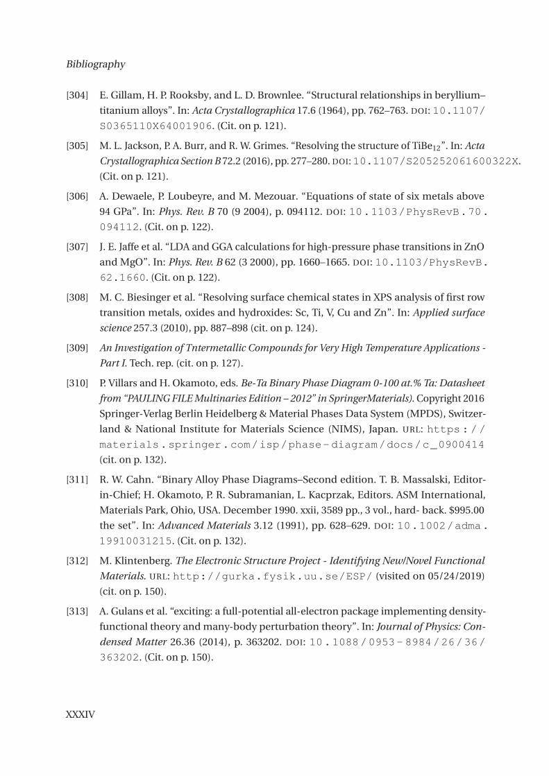
Bibliography
[304] E. Gillam, H. P. Rooksby, and L. D. Brownlee. “Structural relationships in beryllium–
titanium alloys”. In: Acta Crystallographica 17.6 (1964), pp. 762–763. DOI: 10.1107/
S0365110X64001906. (Cit. on p. 121).
[305] M. L. Jackson, P. A. Burr, and R. W. Grimes. “Resolving the structure of TiBe12”. In: Acta
Crystallographica Section B 72.2 (2016), pp. 277–280. DOI:10.1107/S205252061600322X.
(Cit. on p. 121).
[306] A. Dewaele, P. Loubeyre, and M. Mezouar. “Equations of state of six metals above
94 GPa”. In: Phys. Rev. B 70 (9 2004), p. 094112. DOI: 10.1103/PhysRevB.70.
094112. (Cit. on p. 122).
[307] J. E. Jaffe et al. “LDA and GGA calculations for high-pressure phase transitions in ZnO
and MgO”. In: Phys. Rev. B 62 (3 2000), pp. 1660–1665. DOI: 10.1103/PhysRevB.
62.1660. (Cit. on p. 122).
[308] M. C. Biesinger et al. “Resolving surface chemical states in XPS analysis of first row
transition metals, oxides and hydroxides: Sc, Ti, V, Cu and Zn”. In: Applied surface
science 257.3 (2010), pp. 887–898 (cit. on p. 124).
[309] An Investigation of Tntermetallic Compounds for Very High Temperature Applications -
Part I. Tech. rep. (cit. on p. 127).
[310] P. Villars and H. Okamoto, eds. Be-Ta Binary Phase Diagram 0-100 at.% Ta: Datasheet
from “PAULING FILE Multinaries Edition – 2012” in SpringerMaterials). Copyright 2016
Springer-Verlag Berlin Heidelberg & Material Phases Data System (MPDS), Switzer-
land & National Institute for Materials Science (NIMS), Japan. URL: https://
materials.springer.com/isp/phase-diagram/docs/c_0900414
(cit. on p. 132).
[311] R. W. Cahn. “Binary Alloy Phase Diagrams–Second edition. T. B. Massalski, Editor-
in-Chief; H. Okamoto, P. R. Subramanian, L. Kacprzak, Editors. ASM International,
Materials Park, Ohio, USA. December 1990. xxii, 3589 pp., 3 vol., hard- back. $995.00
the set”. In: Advanced Materials 3.12 (1991), pp. 628–629. DOI: 10.1002/adma.
19910031215. (Cit. on p. 132).
[312] M. Klintenberg. The Electronic Structure Project - Identifying New/Novel Functional
Materials. URL: http://gurka.fysik.uu.se/ESP/ (visited on 05/24/2019)
(cit. on p. 150).
[313] A. Gulans et al. “exciting: a full-potential all-electron package implementing density-
functional theory and many-body perturbation theory”. In: Journal of Physics: Con-
densed Matter 26.36 (2014), p. 363202. DOI: 10.1088/0953- 8984/26/36/
363202. (Cit. on p. 150).
XXXIV

Bibliography
[314] The exciting Code. URL: http://exciting-code.org (visited on 05/24/2019)
(cit. on p. 150).
[315] AQR Capital Management and LLC, Lambda Foundry Inc. and PyData Development
Team. pandas: Python Data Analysis Library. URL: https://pandas.pydata.
org (visited on 05/24/2019) (cit. on p. 159).
[316] NumPy developers. NumPy is the fundamental package for scientific computing with
Python. URL: https://www.numpy.org (visited on 05/24/2019) (cit. on p. 159).
[317] J. D. Hunter. “Matplotlib: A 2D graphics environment”. In: Computing In Science &
Engineering 9.3 (2007), pp. 90–95. DOI: 10.1109/MCSE.2007.55 (cit. on p. 159).
[318] S. Behnel, M. Faassenet, and et. al. lxml: the most feature-rich and easy-to-use library
for processing XML and HTML in the Python language. URL: https://lxml.de
(visited on 05/24/2019) (cit. on p. 159).
[319] J. Ellson et al. “Graphviz and dynagraph – static and dynamic graph drawing tools”. In:
GRAPH DRAWING SOFTWARE. Springer-Verlag, 2003, pp. 127–148 (cit. on p. 160).
[320] E. R. Gansner and S. C. North. “An open graph visualization system and its applications
to software engineering”. In: SOFTWARE - PRACTICE AND EXPERIENCE 30.11 (2000),
pp. 1203–1233 (cit. on p. 160).
[321] AT&T labs. Graphviz - Graph Visualization Software. URL: https://graphviz.
gitlab.io (visited on 05/24/2019) (cit. on p. 160).
[322] M. Bastian, S. Heymann, and M. Jacomy. “Gephi: An Open Source Software for Explor-
ing and Manipulating Networks”. In: Third International AAAI Conference on Weblogs
and Social Media (2009), pp. 361–362. ISSN: 14753898. DOI: 10.1136/qshc.2004.
010033. (Cit. on pp. 160–162).
[323] Docker Inc. Enterprise Container Platform for High-Velocity Innovation. URL: https:
//www.docker.com (visited on 05/24/2019) (cit. on p. 160).
[324] DBeaver community. DBeaver: Universal Database Tool. URL: https://dbeaver.
io/ (visited on 05/24/2019) (cit. on p. 160).
[325] J. Egger, C. Pastl, and M. Thompson. Postgres.app: The easiest way to get started with
PostgreSQL on the Mac. URL: https://postgresapp.com (visited on 05/24/2019)
(cit. on p. 160).
[326] J. Egger. Postico: A Modern PostgreSQL Client for the Mac. URL:https://eggerapps.
at/postico/ (visited on 05/24/2019) (cit. on p. 160).
[327] The pgAdmin Development Team. pgAdmin: the most popular and feature rich Open
Source administration and development platform for PostgreSQL. URL: https://
www.pgadmin.org (visited on 05/24/2019) (cit. on p. 160).
XXXV

Bibliography
[328] A. Caudwell. Gource: software version control visualization. URL: https://gource.
io/ (visited on 05/24/2019) (cit. on p. 160).
[329] E. Bonsma. GrandPerspective. URL: http://grandperspectiv.sourceforge.
net (visited on 05/24/2019) (cit. on p. 163).
XXXVI
Publications
Parts of this thesis and results from this work have already been published, or a manuscript
for publication is currently in preparation:
• The contents of chapter 3, The from ab initio data chemical interpreation process for
spectra with sub phase spectra. are published in
International Patent application (05.2018): J. Broeder, Daniel Wortmann, Verfahren zur
Auswertung von Rumpfelektronenspektren
• Parts of chapter 3, The AiiDA-FLEUR package has been published: J. Bröder, D. Wort-
mann, and S. Blügel Using the AiiDA-FLEUR package for all-electron ab initio electronic
structure data generation and processing in materials science, In Extreme Data Workshop
2018 Proceedings, 2019, vol 40, p 43-48
• Source code of the AiiDA-FLEUR package has been released under MIT license on github
and pypi: https://github.com/JuDFTteam/aiida-fleur ; https://pypi.org/project/aiida-
fleur/
• Data of the high-throughput screening of the binary metals (chapter 4) including the
provenance and meta data has been published: J. Bröder, D. Wortmann, and S. Blügel,
JuCLS database of core-level shifts from all-electron density functional theory simulations
for chemical analysis of X-ray photoelectron spectra., Materials CLoud Archive, 2020, doi:
10.24435/materialscloud:3j-p3
• Parts of the results from chapter 3 and 4 are in preparation for publication. Journal
article: manuscript in preparation
XXXVII


Acknowledgements
Arriving here at this state and point in time was a long journey, which was influenced directly
or indirectly by many wonderful and incredible people, to whom I am grateful for being part
of this journey.
First my gratitude goes to Prof. Dr. Stefan Blügel for enabling me to go on this journey at the
outstanding PGI-1/IAS-1. I am thankful for his supervision of my PhD, guidance and support.
Through the participation in the European center of excellence, ’MaX-Materials design at the
Exascale’ together with the various conferences and workshops I was allowed to attend, I was
provided with many chances to broaden my horizon and engaging in scientific collaborations
across borders.
I want to thank Prof. Dr. Christian Linsmeier for his guidance at the outstanding IEK-4,
reviewing and always supporting my work. Without him the cooperation with the IEK-4 and
this work would be totally different.
Furthermore, I thank Prof. Dr. Riccardo Mazzarello for reviewing my work.
Then I thank Dr. Daniel Wortmann for his supervision and guidance throughout my work at
the IAS/PGI and for his efforts on the FLEUR code. I have always enjoyed our discussions,
providing me valuable feedback and further insights.
I also want to thank Dr. H. Rudolf Koslowski, Dr. Nabi Aghdassi, Dr. Timo Dittmar, Nicola
Helfer and Petra Hansen from the IEK-4 for their nice cooperation on the chemical interpreta-
tion of XPS spectra, which motivated me a lot. Through them I received useful insights from
the experimental perspective in our weekly ’friends of surface science’ meetings and their
feedback helped to improve this work. I also thank Dr. Martin Köppen for his discussions on
XPS related to his work.
I thank the FLEUR developer team, for spendings months after months fixing issues related
to my work, Dr. Uliana Alekseeva, Matthias Redis, and especially Dr. Gregor Michalicek, who I
thank also for his friendship, many wonderful discussion and proofreading.
Further I thank Dr. Gustav Bihlmayer for his helpful discussions and for the sharing of his
wisdom and computational resources.
I also want to thank all institute members, including our secretary Ute Winkler and members
XXXIX

Bibliography
of the PGI IT, for the wonderful working atmosphere, many seminars with many fruitful
discussions, out of work events, working with and aside you made this a great time.
Also I like to acknowledge the AiiDA developer team, especially Dr. Giovanni Pizzi, Dr.
Martin Uhrin, Dr. Leopold Talirz and Dr. Sebastiaan Huber but also the plugin developers of
other DFT codes for their professional hard work. It was a pleasure to see some of my ideas
and suggestions advance and finding their way implemented in the AiiDA code base over the
years. Thanks for all the wonderful coding weeks, workshops, brainstorming discussions.
I extend my thanks to other colleagues that I met at scientific events, or corresponded via
email, for their interested, skeptical questions and fruitful discussions concerning this work.
I am also thankful to all the programmer communities out there that write good software
especially open source software from which we all profit a lot. Thanks for your daily work and
efforts, without you my work could only be a shadow of itself. Hereby I thank the national and
international funding agencies for providing us with the resources required to hold up the
status of knowledge and technology and push out further.
In particular, I acknowledge support from European Union H2020-EINFRA-2015-1 pro-
gramme under grant agreement No. 676598 project "MaX - materials at the exascale" and its
successor a H2020-INFRAEDI-2018-1 funded project Grant Agreement n. 824143.
For computing resources I furthermore acknowledge JARA, project jara0172, for computing
time on CLAIX 2016/2017/2018 and JURECA, besides computing time on in-house PGI clus-
ters.
Finally, I am deeply grateful to my loving wife, to my parents, to my wonderful son, siblings
and friends for their endless support with all their heart and understanding. Without you I
would have never arrived at this point.
XL

Eidesstattliche Erklärung
Ich, Jens Bröder erklärt hiermit, dass diese Dissertation und die darin dargelegten Inhalte
die eigenen sind und selbstständig, als Ergebnis der eigenen originären Forschung, generiert
wurden. Hiermit erkläre ich an Eides statt
1. Diese Arbeit wurde vollständig oder größtenteils in der Phase als Doktorand dieser
Fakultät und Universität angefertigt;
2. Sofern irgendein Bestandteil dieser Dissertation zuvor für einen akademischen Ab-
schluss oder eine andere Qualifikation an dieser oder einer anderen Institution verwen-
det wurde, wurde dies klar angezeigt;
3. Wenn immer andere eigene- oder Veröffentlichungen Dritter herangezogen wurden,
wurden diese klar benannt;
4. Wenn aus anderen eigenen- oder Veröffentlichungen Dritter zitiert wurde, wurde stets
die Quelle hierfür angegeben. Diese Dissertation ist vollständig meine eigene Arbeit,
mit der Ausnahme solcher Zitate;
5. Alle wesentlichen Quellen von Unterstützung wurden benannt;
6. Wenn immer ein Teil dieser Dissertation auf der Zusammenarbeit mit anderen basiert,
wurde von mir klar gekennzeichnet, was von anderen und was von mir selbst erarbeitet
wurde;
7. Ein Teil oder Teile dieser Arbeit wurden zuvor veröffentlicht, siehe Publications Auflis-
tung
Forschungszentrum Jülich, Sep 2019
Jens Bröder


Schriften des Forschungszentrums Jülich Reihe Schlüsseltechnologien / Key Technologies
Band / Volume 217 Detection and Statistical Evaluation of Spike Patterns in Parallel Electrophysiological Recordings P. Quaglio (2020), 128 pp ISBN: 978-3-95806-468-3 Band / Volume 218 Automatic Analysis of Cortical Areas in Whole Brain Histological Sections using Convolutional Neural Networks H. Spitzer (2020), xii, 162 pp ISBN: 978-3-95806-469-0 Band / Volume 219 Postnatale Ontogenesestudie (Altersstudie) hinsichtlich der Zyto- und Rezeptorarchitektonik im visuellen Kortex bei der grünen Meerkatze D. Stibane (2020), 135 pp ISBN: 978-3-95806-473-7 Band / Volume 220 Inspection Games over Time: Fundamental Models and Approaches R. Avenhaus und T. Krieger (2020), VIII, 455 pp ISBN: 978-3-95806-475-1 Band / Volume 221 High spatial resolution and three-dimensional measurement of charge density and electric field in nanoscale materials using off-axis electron holography F. Zheng (2020), xix, 182 pp ISBN: 978-3-95806-476-8 Band / Volume 222 Tools and Workflows for Data & Metadata Management of Complex Experiments Building a Foundation for Reproducible & Collaborative Analysis in the Neurosciences J. Sprenger (2020), X, 168 pp ISBN: 978-3-95806-478-2 Band / Volume 223 Engineering of Corynebacterium glutamicum towards increased malonyl-CoA availability for polyketide synthesis L. Milke (2020), IX, 117 pp ISBN: 978-3-95806-480-5

Schriften des Forschungszentrums Jülich Reihe Schlüsseltechnologien / Key Technologies
Band / Volume 224 Morphology and electronic structure of graphene supported by metallic thin films M. Jugovac (2020), xi, 151 pp ISBN: 978-3-95806-498-0 Band / Volume 225 Single-Molecule Characterization of FRET-based Biosensors and Development of Two-Color Coincidence Detection H. Höfig (2020), XVIII, 160 pp ISBN: 978-3-95806-502-4 Band / Volume 226 Development of a transcriptional biosensor and reengineering of its ligand specificity using fluorescence-activated cell sorting L. K. Flachbart (2020), VIII, 102 pp ISBN: 978-3-95806-515-4 Band / Volume 227 Strain and Tool Development for the Production of Industrially Relevant Compounds with Corynebacterium glutamicum M. Kortmann (2021), II, 138 pp ISBN: 978-3-95806-522-2 Band / Volume 228 Complex magnetism of nanostructures on surfaces: from orbital magnetism to spin excitations S. Brinker (2021), III, 208 pp ISBN: 978-3-95806-525-3 Band / Volume 229 High-throughput All-Electron Density Functional Theory Simulations for a Data-driven Chemical Interpretation of X-ray Photoelectron Spectra J. Bröder (2021), viii, 169, XL pp ISBN: 978-3-95806-526-0
Weitere Schriften des Verlags im Forschungszentrum Jülich unter http://wwwzb1.fz-juelich.de/verlagextern1/index.asp


Schlüsseltechnologien / Key TechnologiesBand / Volume 229ISBN 978-3-95806-526-0
Related Documents