High Speed Rail Study Phase 2 Report Appendix Group 1 Travel markets

Welcome message from author
This document is posted to help you gain knowledge. Please leave a comment to let me know what you think about it! Share it to your friends and learn new things together.
Transcript

High Speed Rail Study
Phase 2 Report
Appendix Group 1 Travel markets

In accordance with the east coast high speed rail (HSR) study terms of reference, AECOM and its sub-consultants (Grimshaw, KPMG, SKM, ACIL Tasman, Booz & Co and Hyder, hereafter referred to collectively as the Study Team) have prepared this report (Report). The Study Team has prepared this Report for the sole use of the Commonwealth Government: Department of Infrastructure and Transport (Client) and for a specific purpose, each as expressly stated in the Report. No other party should rely on this Report or the information contain in it without the prior written consent of the Study Team.
The Study Team undertakes no duty, nor accepts any responsibility or liability, to any third party who may rely upon or use this Report. The Study Team has prepared this Report based on the Client’s description of its requirements, exercising the degree of skill, care and diligence expected of a consultant performing the same or similar services for the same or similar study, and having regard to assumptions that the Study Team can reasonably be expected to make in accordance with sound professional principles. The Study Team may also have relied upon information provided by the Client and other third parties to prepare this Report, some of which may not have been verified or checked for accuracy, adequacy or completeness. The Report must not be modified or adapted in any way and may be transmitted, reproduced or disseminated only in its entirety. Any third party that receives this Report, by their acceptance or use of it, releases the Study Team and its related entities from any liability for direct, indirect, consequential or special loss or damage whether arising in contract, warranty, express or implied, tort or otherwise, and irrespective of fault, negligence and strict liability.
The projections, estimation of capital and operational costs, assumptions, methodologies and other information in this Report have been developed by the Study Team from its independent research effort, general knowledge of the industry and consultations with various third parties (Information Providers) to produce the Report and arrive at its conclusions. The Study Team has not verified information provided by the Information Providers (unless specifically noted otherwise) and it assumes no responsibility nor makes any representations with respect to the adequacy, accuracy or completeness of such information. No responsibility is assumed for inaccuracies in reporting by Information Providers including, without limitation, inaccuracies in any other data source whether provided in writing or orally used in preparing or presenting the Report.
In addition, the Report is based upon information that was obtained on or before the date in which the Report was prepared. Circumstances and events may occur following the date on which such information was obtained that are beyond the Study Team’s control and which may affect the findings or projections contained in the Report, including but not limited to changes in ‘external’ factors such as changes in government policy; changes in law; fluctuations in market conditions, needs and behaviour; the pricing of carbon, fuel, products, materials, equipment, services and labour; financing options; alternate modes of transport or construction of other means of transport; population growth or decline; or changes in the Client’s needs and requirements affecting the development of the project. The Study Team may not be held responsible or liable for such circumstances or events and specifically disclaim any responsibility therefore.

High Speed Rail Study Phase 2
Department of Infrastructure and Transport March 2013
Appendix 1A Previous HSR demand studies in Australia and overseas

High Speed Rail Study Phase 2 Appendix 1A
March 2013
Appendix 1A Previous HSR demand studies in Australia and overseas
Prepared for
Department of Infrastructure and Transport
Prepared by AECOM Australia Pty Ltd Level 21, 420 George Street, Sydney NSW 2000, PO Box Q410, QVB Post Office NSW 1230, Australia T +61 2 8934 0000 F +61 2 8934 0001 www.aecom.com ABN 20 093 846 925
March 2013
AECOM in Australia and New Zealand is certified to the latest version of ISO9001 and ISO14001.
© AECOM Australia Pty Ltd (AECOM). All rights reserved.
In accordance with the east coast high speed rail (HSR) study terms of reference, AECOM and its sub-consultants (Grimshaw, KPMG, SKM, ACIL Tasman, Booz & Co and Hyder, hereafter referred to collectively as the Study Team) have prepared this report (Report). The Study Team has prepared this Report for the sole use of the Commonwealth Government: Department of Infrastructure and Transport (Client) and for a specific purpose, each as expressly stated in the Report. No other party should rely on this Report or the information contain in it without the prior written consent of the Study Team. The Study Team undertakes no duty, nor accepts any responsibility or liability, to any third party who may rely upon or use this Report. The Study Team has prepared this Report based on the Client's description of its requirements, exercising the degree of skill, care and diligence expected of a consultant performing the same or similar services for the same or similar study, and having regard to assumptions that the Study Team can reasonably be expected to make in accordance with sound professional principles. The Study Team may also have relied upon information provided by the Client and other third parties to prepare this Report, some of which may not have been verified or checked for accuracy, adequacy or completeness. The Report must not be modified or adapted in any way and may be transmitted, reproduced or disseminated only in its entirety. Any third party that receives this Report, by their acceptance or use of it, releases the Study Team and its related entities from any liability for direct, indirect, consequential or special loss or damage whether arising in contract, warranty, express or implied, tort or otherwise, and irrespective of fault, negligence and strict liability. The projections, estimation of capital and operational costs, assumptions, methodologies and other information in this Report have been developed by the Study Team from its independent research effort, general knowledge of the industry and consultations with various third parties (Information Providers) to produce the Report and arrive at its conclusions. The Study Team has not verified information provided by the Information Providers (unless specifically noted otherwise) and it assumes no responsibility nor makes any representations with respect to the adequacy, accuracy or completeness of such information. No responsibility is assumed for inaccuracies in reporting by Information Providers including, without limitation, inaccuracies in any other data source whether provided in writing or orally used in preparing or presenting the Report. In addition, the Report is based upon information that was obtained on or before the date in which the Report was prepared. Circumstances and events may occur following the date on which such information was obtained that are beyond the Study Team's control and which may affect the findings or projections contained in the Report, including but not limited to changes in 'external' factors such as changes in government policy; changes in law; fluctuations in market conditions, needs and behaviour; the pricing of carbon, fuel, products, materials, equipment, services and labour; financing options; alternate modes of transport or construction of other means of transport; population growth or decline; or changes in the Client's needs and requirements affecting the development of the project. The Study Team may not be held responsible or liable for such circumstances or events and specifically disclaim any responsibility therefore.

High Speed Rail Study Phase 2 Appendix 1A
March 2013
Quality information Document Appendix 1A
Ref 60238250-1.0-REP-0101–1A
Date March 2013

High Speed Rail Study Phase 2 Appendix 1A
March 2013
Table of contents 1.0 Introduction 1 2.0 History of High Speed Rail demand studies in Australia 1
2.1 The studies 1 2.2 The Very Fast Train study (1991) 1 2.3 Speedrail (1999) 3 2.4 East coast Very High Speed Train Scoping study (2001) 4 2.5 Commentary 5
3.0 International HSR demand experience 6 3.1 Introduction 6 3.2 Review of travel demand elasticities 6 3.3 Impacts on rail services 7 3.4 Impacts on air services 7
3.4.1 Air and Rail Competition and Complementarity 7 3.4.2 The VHST study 10
3.5 Impacts on other modes of transport and induced travel 11 3.6 Commentary on the evidence 13 3.7 Accuracy of HSR forecasts 14
4.0 Competitive analysis and success factors 15 4.1 Objectives 15 4.2 International evidence on HSR 15
4.2.1 Air and Rail Competition and Complementarity 15 4.2.2 High Speed Rail Overseas Experience Report (Nash 2011) 16 4.2.3 High Speed Rail – The Competitive Environment (Segal 2006) 16
4.3 Local evidence on HSR 16 4.3.1 Speedrail (SKM & MVA 1999) 16 4.3.2 The current study - phase 2 surveys 18
4.4 Conclusions 20

High Speed Rail Study Phase 2 Appendix 1A
March 2013
1
1.0 Introduction This appendix reviews the previous studies of High Speed Rail (HSR) in Australia and overseas. Section 2 reviews the three previous HSR studies of high speed trains along the east coast of Australia in the past two decades; the Very Fast Train Study1 (1991), the Speedrail project2 (1999) and the East Coast Very High Speed Train Scoping Study3 (2001). The characteristics of the HSR services and the demand forecasts for each project are outlined in this appendix.
The international evidence on the impacts of HSR projects is reviewed in Appendix 1A to provide broad international benchmarks for the assessment of HSR forecasts for the east coast corridor. Whilst overall journey time is an important factor in the success of HSR, evidence on other factors that contribute to the performance of HSR is reviewed in Appendix 1A.
2.0 History of High Speed Rail demand studies in Australia
2.1 The studies There have been three studies of HSR in Australia:
The Very Fast Train Study (1991).
Speedrail (1999). East Coast Very High speed Scoping Study (2001).
2.2 The Very Fast Train study (1991) The Very Fast Train (VFT) study identified a preferred HSR corridor between Sydney and Melbourne, along the Hume Highway (via Canberra). Inter-capital express service journey times were close to three hours between Sydney and Melbourne, two hours between Canberra and Melbourne and one hour between Sydney and Canberra (the service characteristics are given in Table 1).
1 Access Economics, Cost benefit study of the very fast train project, 1990. 2 SKM & VMA, Speedrail Patronage and Revenue Forecasts, supplement to final report, 1999. 3 Arup & TMG, East Coast Very High Speed Train Scoping Study, Phase 1 Preliminary Study Final Report, 2001.

High Speed Rail Study Phase 2 Appendix 1A
March 2013
2
Table 1 The Very Fast Train service
Fares
Express services Express journey times Premium Economy
Sydney-Melbourne 2 hrs 55 mins $217 ($367*)
Full: $130 ($220*)
Discount: $87 ($147*)
Sydney-Canberra 1 hr 5 mins $110 ($170*)
Full: $60 ($102*) Discount: $40 ($68*)
Canberra- Melbourne 1 hr 58 mins $167 ($282*)
Full: $100 ($169*)
Discount: $67 ($113*)
Other stations
Melbourne and Sydney Airports, Campbelltown, Bowral, Goulburn, Yass, Wagga Wagga, Wangaratta, Benalla, Seymour.
Service patterns
Three types of service: non-stop between Sydney and Melbourne, express also stopping at Canberra and about three other stations, and stopping services for other stations. In total 36 services per day in each direction.
* Equivalent fare in today’s prices, assuming base price for study fares is the year of the 1991 study.
The forecasting procedures used a logit mode choice model4 based on a stated preference survey. In 1995, 9.51 million passengers were forecast to use the VFT, of which 40 per cent were on business5. The sources of overall VFT patronage are given in Figure 1, which shows induced travel6 accounted for 30 per cent of VFT patronage, diverted car trips 32 per cent and diverted air trips another 25 per cent. Figure 1 Source of Very Fast Train passengers (1995)
Note: Numbers do not add to 100 per cent due to rounding.
4 Most current Australian and international practice is to model the choice of transport mode using a particular model form referred to as the logit model. For aggregate application such as this it can be related to entropy-maximising concepts while in disaggregate models it arises from random utility theory. 5 ibid. 6 Induced travel is defined as journeys on the high speed rail service which were not diverted from other, existing modes of transport.
25%
32%3%
11%
30%
Air
Car
Train
Coach
Induced

High Speed Rail Study Phase 2 Appendix 1A
March 2013
3
2.3 Speedrail (1999) The Speedrail project identified a preferred HSR corridor between Sydney and Canberra via the Southern Highlands and Goulburn. The fastest inter-capital journey time was one and a half hours between Sydney and Canberra (the service characteristics are given in Table 2). Table 2 The Speedrail service
Fares
Inter-capital service Journey time Business class Economy
Sydney-Canberra 1 hr 30 mins $163 ($240*)
Full: $94 ($138*) Discount:
$70 ($103*)
Other stations
Sydney Airport, Macarthur, Southern Highlands (Bowral), Goulburn.
Service patterns
All trains stop at Sydney Airport and Macarthur, with a more limited service to Goulburn and the Southern Highlands. In total 18 services per day in each direction in 2011 (this is the year for which detailed forecasts are reported – the first year of operation was anticipated to be 2007).
* Equivalent fare in today’s prices, assuming base price for study fares is the year of the study.
The forecasts also used a logit mode choice model based on a stated preference survey. Speedrail annual patronage was forecast to be 4.3 million in 2011, with business travel accounting for approximately 39 per cent of Speedrail passengers7. The sources of Speedrail patronage are given in Figure 2; diverted car trips comprised the majority (46 per cent) of Speedrail passengers, diverted air and rail trips another 19 per cent and 17 per cent respectively, while induced travel was forecast to be just 14 per cent of patronage. The forecasts allow for some train capacity constraints at peak times.
Figure 2 Source of Speedrail passengers (2011)
Note: Numbers do not add to 100 per cent due to rounding
7 SKM & MVA, op. cit., Tables 4.1-4.3.
19%
46%
17%
3%
14%
Air
Car
Train
Coach
Induced

High Speed Rail Study Phase 2 Appendix 1A
March 2013
4
2.4 East coast Very High Speed Train Scoping study (2001) The Scoping study investigated a series of very high speed train (VHST) routes using train technologies providing speeds between 160 kilometres per hour and 500 kilometres per hour. Table 3 gives the details of the 350 kilometres per hour service for a route following the coast north of Sydney and then, south of Sydney, an inland route through Canberra to Melbourne. Journey times of between four and four and a half hours between Brisbane and Sydney and between Sydney and Melbourne were assumed. Table 3 The Very High Speed Train service
Fares
Service Limited stop service journey time* Business Non-business
Sydney-Melbourne 4 hrs 7 mins to 4 hrs 30 mins $143 ($193**) $119 ($161**)
Brisbane-Sydney 4 hrs 24 mins to 4 hrs 33 mins $151 ($204**) $108 ($145**)
Sydney-Canberra 1 hr 48 mins $64 ($86**) $47 ($63**)
Canberra-Melbourne 3 hrs 18mins $129 ($174**) $98 ($132**)
Other stations
Beenleigh, Robina, Coolangatta, Ballina, Grafton, Coffs Harbour, Port Macquarie, Taree, Broadmeadow, Warnervale, Gosford, Hornsby, Strathfield, Sydney Airport, Glenfield, Bowral, Goulburn, Canberra airport, Yass, Cootamundra, Wagga, Albury, Shepparton, Seymour, Melbourne airport. Service patterns Limited stop and all stop services. 16 services each way (an hourly service overall).
*Times varied by the length of the route. ** Equivalent fare in today’s prices, assuming base price for study fares is the year of the study.
For this model, the base year travel demands were derived from the Domestic Tourism Monitor and the International Visitor Survey. The forecast VHST annual patronage was 32.4 million passengers in 20218, of which business travel accounted for 17 per cent9. The sources of overall VHST patronage are given in Figure 3, which shows diverted air trips accounted for 41 per cent of passengers, while diverted car trips and induced travel were 22 per cent and 20 per cent of the patronage respectively. Figure 3 Source of VHST passengers (2021)
8 The study assumed that HSR services would commence operation in 2011, with detailed forecasts being presented in the report for 2021. 9 Arup & TMG, op. cit., Table 9.12, Figure 9.35.
41%
22%
12%
5%
20%
Air
Car
Train
Coach
Induced
High Speed Rail Study Phase 2 Appendix 1A
March 2013
5
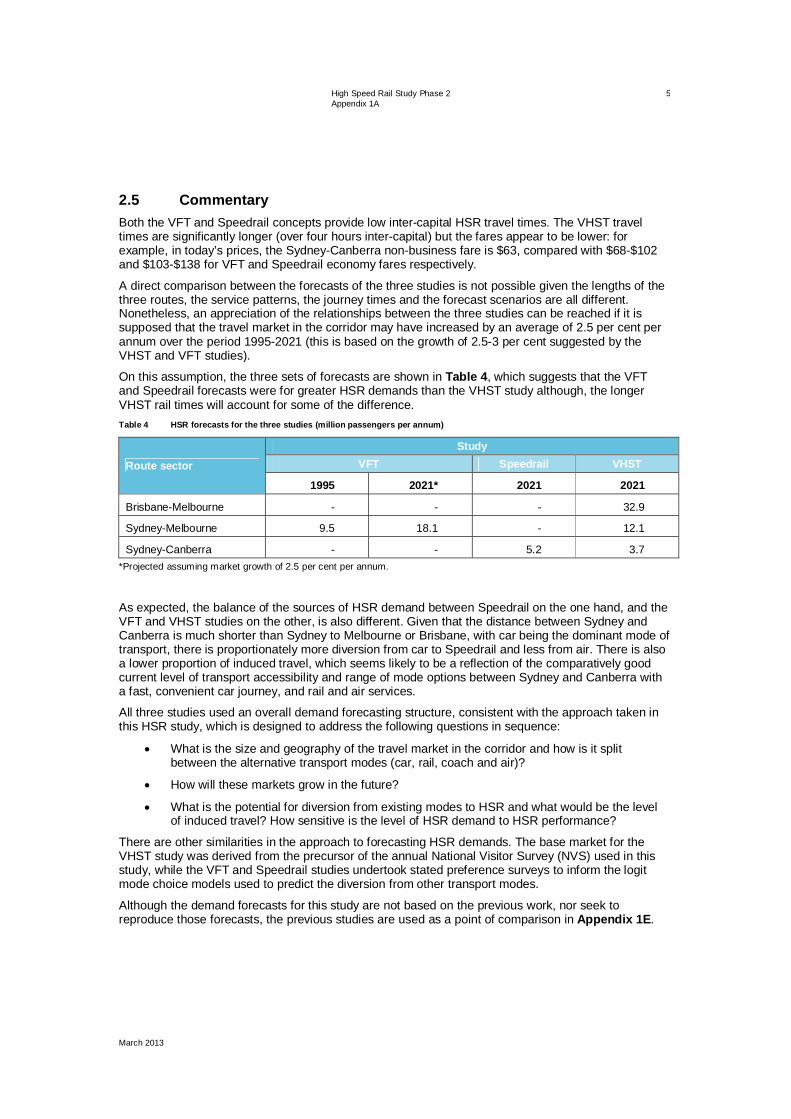
2.5 Commentary Both the VFT and Speedrail concepts provide low inter-capital HSR travel times. The VHST travel times are significantly longer (over four hours inter-capital) but the fares appear to be lower: for example, in today’s prices, the Sydney-Canberra non-business fare is $63, compared with $68-$102 and $103-$138 for VFT and Speedrail economy fares respectively.
A direct comparison between the forecasts of the three studies is not possible given the lengths of the three routes, the service patterns, the journey times and the forecast scenarios are all different. Nonetheless, an appreciation of the relationships between the three studies can be reached if it is supposed that the travel market in the corridor may have increased by an average of 2.5 per cent per annum over the period 1995-2021 (this is based on the growth of 2.5-3 per cent suggested by the VHST and VFT studies).
On this assumption, the three sets of forecasts are shown in Table 4, which suggests that the VFT and Speedrail forecasts were for greater HSR demands than the VHST study although, the longer VHST rail times will account for some of the difference. Table 4 HSR forecasts for the three studies (million passengers per annum)
Route sector
Study VFT Speedrail VHST
1995 2021* 2021 2021
Brisbane-Melbourne - - - 32.9
Sydney-Melbourne 9.5 18.1 - 12.1
Sydney-Canberra - - 5.2 3.7 *Projected assuming market growth of 2.5 per cent per annum.
As expected, the balance of the sources of HSR demand between Speedrail on the one hand, and the VFT and VHST studies on the other, is also different. Given that the distance between Sydney and Canberra is much shorter than Sydney to Melbourne or Brisbane, with car being the dominant mode of transport, there is proportionately more diversion from car to Speedrail and less from air. There is also a lower proportion of induced travel, which seems likely to be a reflection of the comparatively good current level of transport accessibility and range of mode options between Sydney and Canberra with a fast, convenient car journey, and rail and air services.
All three studies used an overall demand forecasting structure, consistent with the approach taken in this HSR study, which is designed to address the following questions in sequence:
What is the size and geography of the travel market in the corridor and how is it split between the alternative transport modes (car, rail, coach and air)?
How will these markets grow in the future?
What is the potential for diversion from existing modes to HSR and what would be the level of induced travel? How sensitive is the level of HSR demand to HSR performance?
There are other similarities in the approach to forecasting HSR demands. The base market for the VHST study was derived from the precursor of the annual National Visitor Survey (NVS) used in this study, while the VFT and Speedrail studies undertook stated preference surveys to inform the logit mode choice models used to predict the diversion from other transport modes.
Although the demand forecasts for this study are not based on the previous work, nor seek to reproduce those forecasts, the previous studies are used as a point of comparison in Appendix 1E.

High Speed Rail Study Phase 2 Appendix 1A
March 2013
6
3.0 International HSR demand experience
3.1 Introduction This section reviews international evidence on the following specific aspects of HSR forecasting:
Travel demand elasticities.
Impacts on existing rail services.
Impacts on air services.
Impacts on other modes and induced travel.
The international evidence is used to provide broad international benchmarks for the assessment of HSR forecasts for the east coast corridor.
3.2 Review of travel demand elasticities The sensitivity of the demand forecasting procedures is measured in part by their response to changes in journey time and costs as measured by the elasticities of demand10. The values in Table 5 are derived from published sources and relate to longer distance and/or inter-city travel demand. The measure of demand is usually trips and it is noted where trip kilometres are used. Where short and long run elasticities are quoted in the literature, the short run (SR) or annual (A) values are quoted, being judged to be more relevant to a study of modal diversion. Induced travel would normally be expected to be a medium term effect, although it is reported that after six months, Eurostar carried 30 per cent induced travel. Long run elasticities may be up to twice the short run values.
The reports listed in the table emphasise that the values are very sensitive to the mode shares for the context being studied. Table 5 Examples of international and local evidence on travel demand elasticities
Elasticity of demand Sources of direct elasticities and recommended average values
Domestic air travel: elasticity to air fare Australian and NSW Governments11: -0.2 to -1.3
Inter-urban rail travel: elasticity to rail fare Wardman (2010)12: -0.6 (SR) Hooper13: -0.7 to -1.0
Prideaux14: -0.6 to -1.2 Inter-urban rail travel: elasticity to rail journey time Wardman (2011)15: -0.3 to -0.9 (SR, A)
Prideaux: -0.9 Inter-urban rail travel: elasticity to rail service headway Wardman (2011): -0.06 to -0.16 (SR, A)
Car travel: elasticity to car journey time Wardman (2011): -0.07 to -0.19 (SR, A) Wallis16: -0.3
Graham17: -0.2 (vehicle kilometre elasticity)
10 For example, if rail fare is increased by (+) 10 per cent and the patronage on rail reduced by (-) nine per cent, then the direct demand elasticity is the ratio of these two changes or -0.9. Values close to zero indicate that the demand is not very sensitive to changes in that aspect of level of service, while values close to or exceeding 1.0 indicate a high level of demand sensitivity. 11 Australian and NSW Governments, Joint study on aviation capacity in the Sydney region, 2012. 12 Wardman, Price Elasticities of Travel Demand in Great Britain, a Meta Analysis, 2010. 13 Hooper, The elasticity of Demand for Travel: a Review, Institution of Transport Studies, Sydney, 1993. 14 Prideaux, Future Demand for Rail Transport, Transport and Energy Conference, Institution of Civil Engineers, London, 1980. 15 Wardman, Review and Meta-Analysis of Time Elasticities of Travel Demand, 2011. 16 Wallis and Schmidt, Australasian travel demand elasticities - an update of the evidence, Australasian Transport Research Forum, 2003. 17 Graham and Glaister, Road traffic demand elasticity estimates: a review, Transport Reviews, May 2004.

High Speed Rail Study Phase 2 Appendix 1A
March 2013
7
3.3 Impacts on rail services Many HSR lines have been developed in corridors already served by rail such as those in France and Japan, which were principally designed to solve railway capacity constraints. With the introduction of HSR, there has been substantial growth in rail patronage in the affected corridors, and there are several studies referencing this growth18.
3.4 Impacts on air services 3.4.1 Air and Rail Competition and Complementarity
This study for the European Commission (EC)19 of the competition between HSR and air in Europe has contributed materially to the HSR demand forecasts. Case studies of eight European air/rail routes (Table 6) were used to understand the key drivers of market share. The eight routes were chosen to reflect a range of characteristics including different journey times, different countries and varying degrees of airline competition. Table 6 The European Commission eight HSR case studies
Route Year
Frankfurt-Koln 2000, 2005
London-Edinburgh 2004
London-Manchester 2005
London-Paris 2002, 2005
Madrid-Barcelona 2002, 2005
Madrid-Seville 2004
Milan-Rome 2005
Paris-Marseilles 1999, 2005
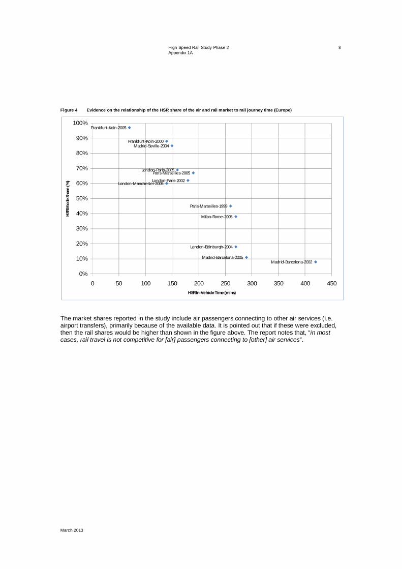
The EC study found that the rail share of air and rail travel varied between the routes from 11 per cent (Madrid-Barcelona) to 97 per cent (Frankfurt-Koln). Figure 4 illustrates the data. Where there is evidence of the share on a particular route varying through time, an additional point is recorded in the figure.
18 See for example: Gourvish, The High Speed Rail Revolution: History and Prospects, HS2 Ltd, 2010; Bilan LOTI, Reseau ferre de France: TGV Atlantique, 2001; LGV Nord, Interconnexion Ile de France, 2005; LGV Rhone-Alpes, 2006; LGV Mediterranee, 2007. 19 Steer Davies Gleave, Air and Rail Competition and Complementarity, European Commission, 2006.
High Speed Rail Study Phase 2 Appendix 1A
March 2013
8
Figure 4 Evidence on the relationship of the HSR share of the air and rail market to rail journey time (Europe)
The market shares reported in the study include air passengers connecting to other air services (i.e. airport transfers), primarily because of the available data. It is pointed out that if these were excluded, then the rail shares would be higher than shown in the figure above. The report notes that, “in most cases, rail travel is not competitive for [air] passengers connecting to [other] air services”.
Frankfurt-Koln-2005
London-Edinburgh-2004
London-Manchester-2005
London-Paris-2005
Madrid-Barcelona-2005
Madrid-Seville-2004
Milan-Rome-2005
Paris-Marseilles-2005
Frankfurt-Koln-2000
London-Paris-2002
Madrid-Barcelona-2002
Paris-Marseilles-1999
0%
10%
20%
30%
40%
50%
60%
70%
80%
90%
100%
0 50 100 150 200 250 300 350 400 450
HSR
Mod
e Sh
are
(%)
HSR In-Vehicle Time (mins)

High Speed Rail Study Phase 2 Appendix 1A
March 2013
9
As part of the study, the factors influencing mode share (journey time, frequency access, etc – see Section 4.2.1) were combined into measures of the utility20 of travel by HSR and air. The relationship between the HSR share and the difference in disutility between rail and air is illustrated in Figure 5. It is clear that the inclusion of the additional factors in the disutility calculation provides a stronger explanation of the variations in HSR shares in this data. The study established a mode choice model which reproduced the variation in HSR mode share with utility difference, represented by the dotted line in Figure 5.
Figure 5 Evidence on the relationship of the HSR share of the air and rail market to the difference in air and rail disutilities (Europe)
20 The convention adopted in the EC study is that travel incurs a negative utility in terms of the time it takes and its cost.
Frankfurt-Koln-2005
London-Edinburgh-2004
London-Manchester-2005
London-Paris-2005
Madrid-Barcelona-2005
Madrid-Seville-2004
Milan-Rome-2005
Paris-Marseilles-2005
Frankfurt-Koln-2000
London-Paris-2002
Madrid-Barcelona-2002
Paris-Marseilles-1999
0%
10%
20%
30%
40%
50%
60%
70%
80%
90%
100%
-200 -150 -100 -50 0 50 100 150
HSR
Mod
e Sh
ares
(%)
Rail Utility Value-Air Utility Value

High Speed Rail Study Phase 2 Appendix 1A
March 2013
10
3.4.2 The VHST study
For the VHST study, information on the split between HSR and air was obtained for 25 city pairs in France, Spain and Japan (Table 7). That information is reproduced in Figure 6 which illustrates that for inter-city travel, there is an evidently close relationship between the rail share and its journey time. On this evidence, if the inter-city rail journey time increases above four hours, then air is likely to retain a majority share of this travel market.
Figure 6 Evidence of the HSR share relationship on the air and rail market to rail journey time (Europe and Asia)
Paris-Dijon
Paris BrusselsMadrid-Cordoba
Tokyo-Nagoya
Ueno-Sendai
Paris-Lyon
Madrid-SevilleTokyo-Osaka
Paris-Valence
Paris-St Etienne Rome-Bologna
Paris-Bordeaux
Paris-London Paris-Marseilles & Stockholm-Gothenburg
Tokyo-Okayama
Paris-Geneva
Madrid-Cadiz
Paris-NimesParis-Montpellier
Madrid-Malaga
Paris-Toulouse
Tokyo-Fukuoka
Tokyo-Hiroshima
Paris-Nice
0%
10%
20%
30%
40%
50%
60%
70%
80%
90%
100%
0 50 100 150 200 250 300 350 400 450
HSR
Mod
e Sh
are
(%)
HSR In-Vehicle Time (mins)

High Speed Rail Study Phase 2 Appendix 1A
March 2013
11
Table 7 Sample of HSR city pairs
City pair Train system Distance (kms)
Tokyo-Nagoya Osaka-Shinkansen 342
Tokyo-Osaka Osaka-Shinkansen 515
Ueno (Tokyo)-Sendai Tohoku-Shinkansen 325
Tokyo-Fukuoka Sanyo-Shinkansen 1,069
Tokyo-Okayama Sanyo-Shinkansen 676
Tokyo-Hiroshima Sanyo-Shinkansen 821
Paris-Valence TGV 527
Paris-St Etienne TGV 489
Paris-Dijon TGV 285
Paris-Geneva TGV 410*
Paris-Nimes TGV 690
Paris-Marseilles TGV 750
Paris-Montpellier TGV 740
Paris-Toulouse TGV 827
Paris-Bordeaux TGV 567
Paris-Lyon TGV 430
Paris-Nice TGV 1,003
Rome-Bologna AV 318
Paris-Brussels Thalys 312
Paris-London Eurostar 494
Stockholm-Gothenburg X2000 455
Madrid-Cadiz Talgo 628
Madrid-Cordoba AVE 343
Madrid-Seville AVE 471
Madrid-Malaga AVE 414* Source: table 9.24, VHST, 2001. *Straight line distance estimate.
3.5 Impacts on other modes of transport and induced travel Reliable data on the impacts of HSR on car and coach travel and the level of induced travel is far less comprehensive.
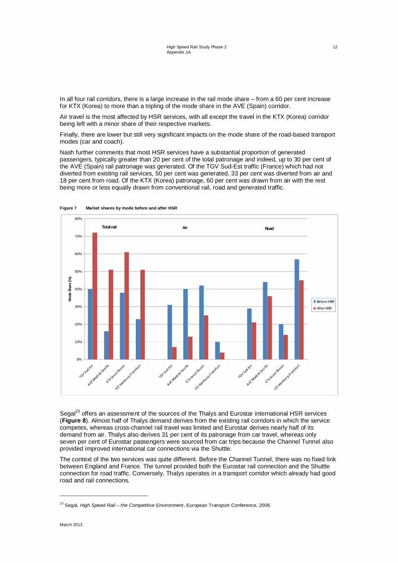
Nash21, in his report on HSR Overseas Experience for phase 1 of this study, reported the impacts of French, Spanish and Korean HSR services on other modes of transport and induced travel. Fundacion BBVA22 provides additional data for German HSR services. This information is displayed in Figure 7. The four rail corridors are: the French TGV service between Paris and Lyons (TGV Sud-Est), the Spanish AVE service between Madrid and Seville, the Korean KTX service between Seoul and Busan, and the German ICE service between Hamburg and Frankfurt.
21 Nash, HSR Overseas experience Report, High Speed Rail Study Phase 1, 2011. 22 Fundacion BBVA, Economic Analysis of High Speed rail in Europe, 2009.
High Speed Rail Study Phase 2 Appendix 1A
March 2013
12
In all four rail corridors, there is a large increase in the rail mode share – from a 60 per cent increase for KTX (Korea) to more than a tripling of the mode share in the AVE (Spain) corridor.
Air travel is the most affected by HSR services, with all except the travel in the KTX (Korea) corridor being left with a minor share of their respective markets.
Finally, there are lower but still very significant impacts on the mode share of the road-based transport modes (car and coach).
Nash further comments that most HSR services have a substantial proportion of generated passengers, typically greater than 20 per cent of the total patronage and indeed, up to 30 per cent of the AVE (Spain) rail patronage was generated. Of the TGV Sud-Est traffic (France) which had not diverted from existing rail services, 50 per cent was generated, 33 per cent was diverted from air and 18 per cent from road. Of the KTX (Korea) patronage, 60 per cent was drawn from air with the rest being more or less equally drawn from conventional rail, road and generated traffic.
Figure 7 Market shares by mode before and after HSR
Segal23 offers an assessment of the sources of the Thalys and Eurostar international HSR services (Figure 8). Almost half of Thalys demand derives from the existing rail corridors in which the service competes, whereas cross-channel rail travel was limited and Eurostar derives nearly half of its demand from air. Thalys also derives 31 per cent of its patronage from car travel, whereas only seven per cent of Eurostar passengers were sourced from car trips because the Channel Tunnel also provided improved international car connections via the Shuttle.
The context of the two services was quite different. Before the Channel Tunnel, there was no fixed link between England and France. The tunnel provided both the Eurostar rail connection and the Shuttle connection for road traffic. Conversely, Thalys operates in a transport corridor which already had good road and rail connections.
23 Segal, High Speed Rail – the Competitive Environment, European Transport Conference, 2006.
0%
10%
20%
30%
40%
50%
60%
70%
80%
Mod
e Sh
are
(%)
Before HSR
After HSR
Total rail Air Road

High Speed Rail Study Phase 2 Appendix 1A
March 2013
13
Figure 8 Sources of Eurostar and Thalys rail demands
The Chinese experience (summarised in Table 8) demonstrates the level of induced travel by HSR is, based on the available evidence, estimated to be very high at 40-65 per cent depending on the context.24
Table 8 Impacts of HSR lines in China
Route HSR patronage (million pax/annum)
Diverted from other modes
Diverted from road or induced
Wuhan-Guangzhou 20 50% rail 5% air 45% (mainly induced)
Beijing-Tianjin 25 16% rail 4% bus 80% (at least 65% induced)
Changchun-Jilin 10 10% rail 20% bus 70% (40-50% induced)
Amos et al.25have in addition to reviewing the French and Japanese contexts, suggested that in Germany, 65 per cent of HSR patronage was drawn from existing rail services and of the remainder, 20 per cent was diverted from car and 15 per cent from air with very small numbers of generated trips. They suggest that when Eurostar was first introduced, it was established that 25-30 per cent of the total patronage was generated.
3.6 Commentary on the evidence Considerable evidence has been assembled in the international literature on the impacts of HSR on air travel, and the EC study has investigated the issue in some depth. In Figure 9, the evidence on the HSR:air shares from the EC and VHST studies, and the report by Nash, has been combined to provide a comprehensive and evidently consistent picture of the relationship between the HSR share and train journey time.
However, the analysis in the EC study shows that factors other than HSR journey time must be allowed for in order to explain the full variations in the HSR:air shares. They measure the ‘disutility’ of both air and rail by combining in-vehicle journey times, with service frequency and check-in time, punctuality and reliability, terminal accessibility, price and service quality.
There appears to be less comprehensive information available on the other demand impacts of HSR, the diversion from car and induced travel, although the evidence confirms that both are significant.
24 Bullock et al, High Speed Rail – The First three Years: Taking the Pulse of China’s Emerging Program, China Transport Topics No. 4, World Bank, 2012. 25 Amos et al, High Speed Rail: the Fast Track to Economic Development?, World Bank, 2010.
12%
49%
12%
7%
20%
Eurostar
Train
Air
Coach
Car
Induced
47%
8%3%
31%
11%
Thalys
Train
Air
Coach
Car
Induced

High Speed Rail Study Phase 2 Appendix 1A
March 2013
14
Diversion from car is significant in all of the evidence reviewed. The most common range is around 20-30 per cent, including TGV Sud-Est, Thalys and the German high speed trains. Diversion rates lower than this are suggested for Eurostar (because of its atypical context) and for the Chinese railways and KTX, both of which have very low current car shares.
Most HSR services have a substantial proportion of generated passengers. However, the range is wide from relatively low levels of induced travel quoted for the German railways, Thalys and KTX, through the 20-30 per cent range for Eurostar and AVE, to the very high levels of TGV Sud-Est and the Chinese HSR system. Part of the explanation of these variations is likely to be the quality and extent of the transport system in the corridor prior to the introduction of HSR.
Figure 9 Evidence of the HSR share relationship on the air and rail market to rail journey time (combined EC and VHST studies and
Nash evidence)
3.7 Accuracy of HSR forecasts Finally, it is noted that concerns over the accuracy of rail project forecasting are also raised in the literature.
The UK National Audit Office26 has recently released its report on High Speed 1, in which it comments that “[passenger] numbers, however, between 2007 and 2011 have been, on average, one third of the level that LCR forecast in 1995 for its bid … [passenger] numbers were also around 30% below the Department’s 1998 forecasts, before it guaranteed the project debt”.
Bullock et al. also observes that “patronage on some of the [Chinese high speed rail] lines remains substantially below the opening-year forecasts developed in their respective feasibility studies”.
Conversely, Albalate et al.27 report that the demand forecasts for the Tokyo-Osaka Shinkansen line underestimated patronage.
26 National Audit Office, UK, The completion and sale of High Speed 1, 2012. 27 Albalate et al, High Speed rail: Lessons for Policy Makers from Experiences Abroad, IREA University of Barcelona, 2010.
Paris-Dijon
Paris BrusselsMadrid-Cordoba
Tokyo-Nagoya
Ueno-Sendai
Paris-Lyon
Madrid-SevilleTokyo-Osaka
Paris-Valence
Paris-St Etienne Rome-Bologna
Paris-Bordeaux
Paris-London
Paris-Marseilles & Stockholm-Gothenburg
Tokyo-Okayama
Paris-Geneva
Madrid-Cadiz
Paris-NimesParis-Montpellier
Madrid-Malaga
Paris-Toulouse
Tokyo-Fukuoka
Tokyo-Hiroshima
Paris-Nice
Frankfurt-Koln-2005
London-Edinburgh-2004
London-Manchester-2005
London-Paris-2005
Madrid-Barcelona-2005
Madrid-Seville-2004
Milan-Rome-2005
Paris-Marseilles-2005
Frankfurt-Koln-2000
London-Paris-2002
Madrid-Barcelona-2002
Paris-Marseilles-1999
Brussels-London
Seoul-Busan
Madrid-Barcelona
Tokyo-Okayama
Paris-Amsterdam
0%
10%
20%
30%
40%
50%
60%
70%
80%
90%
100%
0 50 100 150 200 250 300 350 400 450
HSR
Mod
e Sh
are
(%)
HSR In-Vehicle Time (mins)
VHST Study
EC Study
Nash paper

High Speed Rail Study Phase 2 Appendix 1A
March 2013
15
Of the five routes reported in the Bilan Loti reports which were reviewed, two of the routes were forecast reasonably accurately and for three the demand over-estimated the impact of the TGV route. Of the latter, TGV Nord was affected by the Eurostar forecasting errors.
With these concerns over the accuracy of rail project forecasting in mind, where there were uncertainties in the modelling, conservative decisions were taken, and the forecasts for the east coast HSR line have been benchmarked against the international evidence (see Appendix 1E).
4.0 Competitive analysis and success factors
4.1 Objectives To inform the design of the HSR transport products, the key HSR success factors for market segments drawn from local and international literature are reviewed in this section to determine the factors influencing the choice of HSR and the surveys on this study.
4.2 International evidence on HSR 4.2.1 Air and Rail Competition and Complementarity
This paper for the EC28 discusses the effectiveness of HSR in relation to its competitiveness with air. The paper includes a discussion of the ‘drivers of market share’ based on a review of eight European routes. The study conclusions on market share are reproduced below.
The case studies show that rail journey time is by far the most important factor determining rail/air market share. In principle, it is better to examine the difference between rail and air journey time rather than just the rail journey time, although in practice this may not make much difference to the results, because air journey times do not vary as much between routes as rail journey times do. The correlation is improved if we look at generalised journey time rather than purely at scheduled in-vehicle journey time. Generalised journey time takes into account whether each mode offers a high or low frequency service and also any check-in time. We found that generalised journey time explained most of the difference in rail market share across the routes that we studied.
However, we found that even allowing for generalised journey time variations there were still significant variations in market share across the routes that we studied. There were a number of reasons for this. Punctuality and reliability appeared to be very important factors in determining market share, and a number of the operators with whom we consulted emphasised that these were as important as journey time. The accessibility of terminals is a very important factor in determining market share on individual routes but as this is not within the control of the operators within the short term, it is not a factor that they emphasised. In contrast, the service quality available on board and in terminals did not seem to be a particularly important factor determining market share. However, this was in part because there was not much difference in the service quality offered by the different operators, except in first/business class which represents a small proportion of passengers.
Although there was some evidence that price was an important factor in determining market share, this was less clear than might have been expected. Rail achieved a high market share on some routes (such as London-Paris) despite relatively high prices. The main route on which price seemed to have had a significant effect on market share was the London-Edinburgh route, where the existence of a high frequency low cost airline service had caused significant switch from rail. In evaluating the affect [sic] of price variations, we also need to consider the existence of alternative lower cost modes of transport. For example, the high market share achieved by rail on the Rome-Milan route is the result of both relatively low rail fares and the lack of any lower priced alternative to rail transport (such as a bus service).
28 Steer Davies Gleave, Air and Rail Competition and Complementarity, European Commission, 2006.
High Speed Rail Study Phase 2 Appendix 1A
March 2013
16
In summary, the paper argues that the main factor which drives HSR market share is the rail journey time. Check-in time is considered part of journey time, and the absence of the need for a long check-in for HSR is an advantage. It is also noted that rail must have a competitive service frequency.
Steer Davies Gleave observes that other factors accounted for the variations in mode shares for the routes which they studied. These factors were:
The time and cost involved in accessing air and rail terminals: aside from journey time, accessibility to the competing modes of transport is one of the most important factors.
Price and ticket conditions, in which the low cost airlines and yield management are significant issues.
Reliability and punctuality, whose importance rail operators emphasised.
Service quality on board and at terminals is thought to be of diminishing importance and not considered relevant by operators, but this may simply be because there are common standards used on competing modes.
The availability of alternative (lower cost) modes, regarding which Steer Davies Gleave mentions coach and private car.
Interchange is also an important consideration, with rail travel generally not competitive for passengers connecting to air services.
In regard to some of these factors, the presence of competition from low cost airlines is important.
4.2.2 High Speed Rail Overseas Experience Report (Nash 2011)29
The findings of Nash concur with the Steer Davies Gleave report on journey time, reliability, accessibility of stations (particularly city centre stations), airport check-in times and waiting times generally, competitive fares, yield management and seat reservations systems all mentioned.
4.2.3 High Speed Rail – The Competitive Environment (Segal 2006)30 Similarly, in this paper presented at the European Transport conference, it is argued that journey times are critical. The paper states that business travellers seek an uninterrupted journey (with the ability to work on the train), quality of service (catering, etc) and a ‘turn up and go’ experience with the associated service frequency. The paper also raises the issue of fares, accessibility and check-in.
4.3 Local evidence on HSR 4.3.1 Speedrail (SKM & MVA 1999) Extensive market research was undertaken for the Speedrail project, including in-depth interviews and focus groups to investigate consumer preferences and perceptions of existing travel modes and HSR.
Table 9 is an extract from the Speedrail report, which details the advantages and disadvantages identified by survey respondents regarding their current modes of transport for journeys between Sydney and Canberra.
When questioned about the Speedrail service offering, the participants focused on cost, regularity and reliability, their views being summarised in Table 10 (extracted from the Speedrail report).
29 Ibid. 30 Ibid.

High Speed Rail Study Phase 2 Appendix 1A
March 2013
17
Table 9 Speedrail - advantages and disadvantages of existing modes of transport between Sydney and Canberra
Car Train
Advantages - Convenient - Easier with children - Flexibility - Need for car at destination - because of
equipment , location of the ultimate destination, etc
- Size of the travelling group/family - Luggage - For leisure trips and/or bringing the family up to
join the respondent “you’d always drive”; where a family is involved the availability of a car “at the other end” is invaluable
- It was felt that it was difficult to justify the expense of flying for a 3 hour leisure driving trip
Advantages - Cost - Fare - Duration and location of the visit - Not having to look for parking
Disadvantages - Uncomfortable seats, the bumpy ride and the
poor food - Safety at railway stations - Having to change trains was not desirable - Being tied to a schedule
Air
Advantages For business trips: - Cost not a big issue, fares were either paid by the company or funded by frequent flyer points which were
gained on other “longer” flights - Plane travel is considered to be more relaxing than driving when you are working and “you can work on
the plane” - Membership of Qantas Club/Golden Wing is another important influence - ability to make phone calls,
have meetings, have a shower “to freshen up” - Ability to purchase plane tickets in advance which reduces the fare (although this means there is less
flexibility in your bookings later)
Disadvantages - Check-in time - Total time including access - Expensive - Cramped and stressful

High Speed Rail Study Phase 2 Appendix 1A
March 2013
18
Table 10 Speedrail - perceptions of HSR
HSR
Advantages Overall HSR was perceived as a service that would be: - Convenient - Better than the existing train service - Reliable timetable - Speedy - Would be more relaxed and more refreshed
upon arrival - Could do work on the train, can get paperwork in
order for meetings, be able to use their electronic equipment, including their mobile telephone, as long as they were not disturbed by children
- Reliability of timetable - Could sell travel by HSR to companies and they
could reduce their fleet of vehicles
Inhibiting features - Cost was seen as a potential disadvantage; off
peak rates were seen as necessary to promote usage by “ordinary” people; for leisure trips particularly
- The need to “keep to a schedule” was another issue raised concerning HSR versus car travel
- Travel in groups - Need for car at the other end - Frequent modal interchanges
Issues raised: - Security at stations and on trains - Access at stations: buses and taxis meeting trains, secure parking, car rentals, shuttle bus services - Ticketing arrangements - Timetabling schedules and frequencies – being able to catch a train when you needed it - Service at stations: waiting areas, baby changing rooms and facilities to look after unaccompanied
children, money exchange (for tourists), luggage trolleys, speedy reclaim of luggage and no luggage limits - On train services, including services for business people (faxes, places to plug in computers, modems,
ability to use mobile phones, collect e-mails), buffet car, a lounge area or observation carriage, video screen, music, bar
- Comfortable seats - Luggage arrangements: no luggage restrictions, provision for luggage, being able to book in the luggage
and not have to carry it, the amount of hand luggage you could take on (if significantly more than on a plane this would be a decided advantage), the amount of “book-on” luggage you could carry (e.g. for trade displays) and the speed with which this luggage can be retrieved at the end of the journey
- The smoothness of the ride - Helpful staff - Cleanliness
4.3.2 The current study - phase 2 surveys
The initial focus groups and the stated preference (SP) survey (Appendix 1D) for this study investigated why people would not choose to use HSR and what they would value most about HSR.
More than half the travellers interviewed in the main SP survey (travelling by air, car and conventional rail) did not consider that there were any current alternative modes possible for their journey. However, given a journey in the HSR catchment, most (81 per cent) of the respondents from the main SP survey would consider HSR.
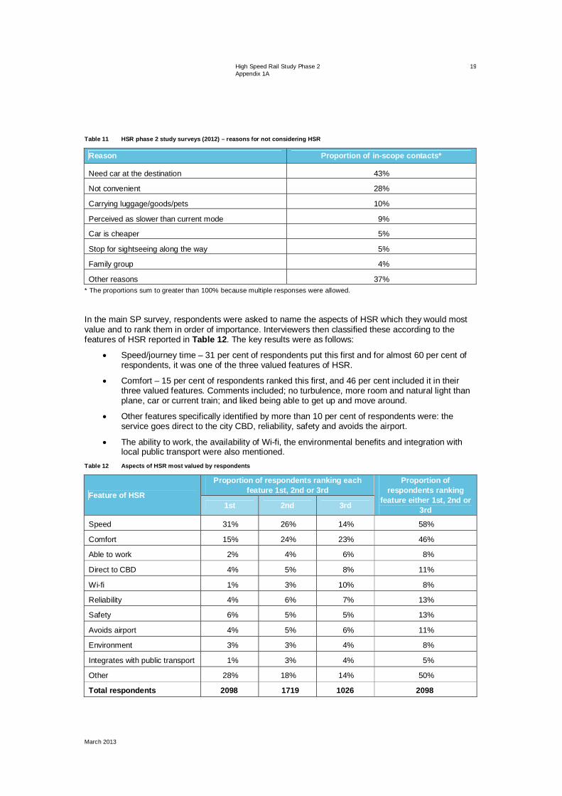
Of those that would not consider HSR, the main reasons are given in Table 11. The SP survey results show that just under 80 per cent of respondents used their car for the journey. The predominant reasons for not considering HSR were inconvenience and the need for a car at the destination. Other specific reasons included: carrying luggage, goods or pets; slower than current mode; car is cheaper; sightseeing stops and family group travel.
The focus groups also suggested that the constraint of company travel policies prohibits consideration of HSR.
High Speed Rail Study Phase 2 Appendix 1A
March 2013
19
Table 11 HSR phase 2 study surveys (2012) – reasons for not considering HSR
Reason Proportion of in-scope contacts*
Need car at the destination 43%
Not convenient 28%
Carrying luggage/goods/pets 10%
Perceived as slower than current mode 9%
Car is cheaper 5%
Stop for sightseeing along the way 5%
Family group 4%
Other reasons 37% * The proportions sum to greater than 100% because multiple responses were allowed.
In the main SP survey, respondents were asked to name the aspects of HSR which they would most value and to rank them in order of importance. Interviewers then classified these according to the features of HSR reported in Table 12. The key results were as follows:
Speed/journey time – 31 per cent of respondents put this first and for almost 60 per cent of respondents, it was one of the three valued features of HSR.
Comfort – 15 per cent of respondents ranked this first, and 46 per cent included it in their three valued features. Comments included; no turbulence, more room and natural light than plane, car or current train; and liked being able to get up and move around.
Other features specifically identified by more than 10 per cent of respondents were: the service goes direct to the city CBD, reliability, safety and avoids the airport.
The ability to work, the availability of Wi-fi, the environmental benefits and integration with local public transport were also mentioned.
Table 12 Aspects of HSR most valued by respondents
Feature of HSR
Proportion of respondents ranking each feature 1st, 2nd or 3rd
Proportion of respondents ranking
feature either 1st, 2nd or 3rd 1st 2nd 3rd
Speed 31% 26% 14% 58%
Comfort 15% 24% 23% 46%
Able to work 2% 4% 6% 8%
Direct to CBD 4% 5% 8% 11%
Wi-fi 1% 3% 10% 8%
Reliability 4% 6% 7% 13%
Safety 6% 5% 5% 13%
Avoids airport 4% 5% 6% 11%
Environment 3% 3% 4% 8%
Integrates with public transport 1% 3% 4% 5%
Other 28% 18% 14% 50%
Total respondents 2098 1719 1026 2098

High Speed Rail Study Phase 2 Appendix 1A
March 2013
20
Additionally, the focus groups suggested as reasons for considering HSR:
The ability to retain control of luggage.
Less wear and tear on the car.
4.4 Conclusions The body of evidence examining factors that drive the take-up of HSR services indicates that the main determinant of HSR mode share is the journey time of HSR relative to the competing modes. Consumers perceive access times and check-in as part of the overall journey time in making their decision. This being the case, a successful HSR service requires competitive journey times complemented by:
Convenient station access/egress arrangements.
Convenient timetabling (frequencies and service patterns).
An appropriate fare structure (that includes yield management).
Furthermore, there is a clear and consistent theme running through the literature that identifies the main attractions of HSR to be:
Ability to use time productively (business or leisure activities).
Access to city centres, including avoiding congestion.
Comfort and the ability to relax.
Similarly, the disadvantages are consistently identified as:
Connections to the final destination (including the need for a car at the destination).
Wait time, interchanges etc.
Unreliability.
Carrying heavy items of luggage.
It is also apparent that there are specific factors influencing the decisions of business travellers such as company travel policies and the availability of business lounges.

High Speed Rail Study Phase 2
Department of Infrastructure and Transport March 2013
Appendix 1B Use of the National Visitor Survey data

High Speed Rail Study Phase 2 Appendix 1B
March 2013
Appendix 1B Use of the National Visitor Survey data
Prepared for
Department of Infrastructure and Transport
Prepared by AECOM Australia Pty Ltd Level 21, 420 George Street, Sydney NSW 2000, PO Box Q410, QVB Post Office NSW 1230, Australia T +61 2 8934 0000 F +61 2 8934 0001 www.aecom.com ABN 20 093 846 925
March 2013
AECOM in Australia and New Zealand is certified to the latest version of ISO9001 and ISO14001.
© AECOM Australia Pty Ltd (AECOM). All rights reserved.
In accordance with the east coast high speed rail (HSR) study terms of reference, AECOM and its sub-consultants (Grimshaw, KPMG, SKM, ACIL Tasman, Booz & Co and Hyder, hereafter referred to collectively as the Study Team) have prepared this report (Report). The Study Team has prepared this Report for the sole use of the Commonwealth Government: Department of Infrastructure and Transport (Client) and for a specific purpose, each as expressly stated in the Report. No other party should rely on this Report or the information contain in it without the prior written consent of the Study Team. The Study Team undertakes no duty, nor accepts any responsibility or liability, to any third party who may rely upon or use this Report. The Study Team has prepared this Report based on the Client's description of its requirements, exercising the degree of skill, care and diligence expected of a consultant performing the same or similar services for the same or similar study, and having regard to assumptions that the Study Team can reasonably be expected to make in accordance with sound professional principles. The Study Team may also have relied upon information provided by the Client and other third parties to prepare this Report, some of which may not have been verified or checked for accuracy, adequacy or completeness. The Report must not be modified or adapted in any way and may be transmitted, reproduced or disseminated only in its entirety. Any third party that receives this Report, by their acceptance or use of it, releases the Study Team and its related entities from any liability for direct, indirect, consequential or special loss or damage whether arising in contract, warranty, express or implied, tort or otherwise, and irrespective of fault, negligence and strict liability. The projections, estimation of capital and operational costs, assumptions, methodologies and other information in this Report have been developed by the Study Team from its independent research effort, general knowledge of the industry and consultations with various third parties (Information Providers) to produce the Report and arrive at its conclusions. The Study Team has not verified information provided by the Information Providers (unless specifically noted otherwise) and it assumes no responsibility nor makes any representations with respect to the adequacy, accuracy or completeness of such information. No responsibility is assumed for inaccuracies in reporting by Information Providers including, without limitation, inaccuracies in any other data source whether provided in writing or orally used in preparing or presenting the Report. In addition, the Report is based upon information that was obtained on or before the date in which the Report was prepared. Circumstances and events may occur following the date on which such information was obtained that are beyond the Study Team's control and which may affect the findings or projections contained in the Report, including but not limited to changes in 'external' factors such as changes in government policy; changes in law; fluctuations in market conditions, needs and behaviour; the pricing of carbon, fuel, products, materials, equipment, services and labour; financing options; alternate modes of transport or construction of other means of transport; population growth or decline; or changes in the Client's needs and requirements affecting the development of the project. The Study Team may not be held responsible or liable for such circumstances or events and specifically disclaim any responsibility therefore.

High Speed Rail Study Phase 2 Appendix 1B
March 2013
Quality information Document Appendix 1B
Ref 60238250-1.0-REP-0101–1B
Date March 2013

High Speed Rail Study Phase 2 Appendix 1B
March 2013
Table of contents 1.0 Introduction and objectives 1 2.0 The study area 1 3.0 Establishing the base travel market in the study area 2
3.1 NVS data background 2 3.2 NVS data used for this study 2
4.0 The base market 6 5.0 Verification of the base market 12
5.1 Background 12 5.2 Verification against independent rail and air travel data 12 5.3 Verification against independent car travel data: the registration number survey 13
5.3.1 The registration number survey 13 5.3.2 Verification of the base market against the number plate data 15
5.4 Distributions of travel origins and destinations between CBDs and suburban areas in major metropolitan areas 16
6.0 Verification conclusions 20

High Speed Rail Study Phase 2 Appendix 1B
March 2013
1
1.0 Introduction and objectives The demand forecasting procedures rely on an appreciation of the current patterns of travel demand along the east coast – it is these journeys, projected into the future, which High Speed Rail (HSR) would potentially serve. To this end, the size of the current travel market for the east coast study area was determined by origin and destination, trip purpose and transport mode from National Visitor Survey (NVS) data collected by Tourism Research Australia.
As the current travel market forming the basis of the HSR forecasts, the resulting market estimates were also verified against independent information, which included a specially-commissioned survey of interurban road traffic patterns.
2.0 The study area With a preferred corridor established at the end of phase 1, the study area for the phase 2 demand forecasting focused on the preferred HSR corridor. This is illustrated in Figure 1, which also shows the sector breakdown which is used in the analyses of the base travel market. Figure 1 The study area showing the analysis sectors
1. Melbourne 2. Intermediate 3. Canberra 4. Intermediate 5. Sydney 6. Intermediate 7. Newcastle 8. Intermediate 9. Gold Coast 10. Brisbane

High Speed Rail Study Phase 2 Appendix 1B
March 2013
2
3.0 Establishing the base travel market in the study area
3.1 NVS data background Since 2005, interviews have been conducted on an annual basis with approximately 120,000 Australian residents, aged 15 years and over. This sample was increased from 80,000 interviews annually between 1998 and 2004 in order to enhance estimates for smaller states/territories at the regional level. Respondents are interviewed in their homes using random digit dialling and a Computer Assisted Telephone Interviewing system1. Respondents interviewed in the NVS are randomly sampled to be representative of the Australian population, based on place of residence, age and gender.
Interviews are conducted with people who have travelled for purposes including holiday, visiting friends and relatives, business, education and employment. The survey questions include the destination, purpose, mode of transport, travel party and demographics.
Expansion weights for the NVS are calculated on an individual trip basis. They take into account the age, gender and place of origin of the respondent, the size of the household in which they live, month of travel, the recall period applicable to the trip (for example, seven days for day trips, 28 days for overnight trips and three months for overseas trips) and the number of interviews with a return date in this recall period. The NVS is benchmarked to population estimates of those aged 15 years and over.
3.2 NVS data used for this study The phase 2 base travel demands have been based on 11 years of NVS data collected between 2000 and 2010. This data comprises a total sample of over 146,000 day trips and overnight trips, which represents when expanded, 152 million trips in the base travel market in 2009.
The base market encompasses trips greater than 50 kilometres within the study area with an end in one of the major towns and cities: Melbourne, Sydney, Brisbane, Canberra, Newcastle, Wollongong and Gold Coast.
The following trips are considered unlikely to transfer to HSR and have been omitted from the base market:
Short distance (less than 50 kilometres) and intra-urban/metropolitan area travel, amounting to 37.9 million trips annually.
Trips within the regional ‘intermediate’ sectors, mainly by car between small towns and rural areas, amounting to 21.8 million trips annually.
Longer trips between these ‘intermediate’ sectors, amounting to 5.4 million trips annually. Longer trips may transfer to HSR and, to this extent, HSR forecasts are conservative.
Journeys to and from places that are external to the study area.
The resulting estimated size of the annual base market of trips2 in the east coast corridor in 2009 is 152 million.
In combining the NVS data for all 11 years, more weight was placed on the more recent surveys and those with larger survey samples, and the combined data base was controlled to reproduce the overall characteristics of 2009. The NVS omits the travel of children under 15 years old and that of international visitors and factors have been devised from NVS data and other information provided by the Bureau of Infrastructure, Transport and Regional Economics (BITRE) to estimate this missing travel.
All statistics relating to the base market in this section, in the tables and figures, are derived from the processed NVS data. All tables and figures in the remainder of this section are derived from the NVS data as processed for this study and thus relate to the base travel market. Except for Figure 2 to
1 The NVS was introduced in January 1998 replacing the Domestic Tourism Monitor. The descriptions which follow are taken from published information by Tourism Research Australia. 2 A trip is a journey from one place to another by a single person. If three people travel together, these account for three trips. Most journeys involve an outbound and return journey, counting as two separate trips.

High Speed Rail Study Phase 2 Appendix 1B
March 2013
3
Figure 5, which tabulate the (unexpanded) interviews, all tables and figures are of expanded data (152 million trips).
Concerning the broad characteristics of the travel and travellers, 58 per cent were daytrips and 41 per cent involved an overnight stay (Figure 2), most overnight stays being for one or two nights. Figure 2 Distribution of east coast travel demand by nights away
Note: Number may not add to 100 per cent due to rounding
Approximately 14 per cent were trips on business (Figure 3), the remainder being for other purposes, almost 70 per cent being for holidays or visiting friends and relatives.
Figure 3 Distribution of east coast travel demand by the purpose of the trip
Information on the travel group is available for overnight stays (Figure 4). People travelling alone account for almost 30 per cent of all such trips, with a further 27 per cent being an adult couple (related), family groups account for 20 per cent of all journeys.
58%
12%
11%
6%
4%8%
Day trips
1
2
3
4
5 or more
33%
35%
3%
5%
4%
3%
3%
14%
Visiting friends and relatives
Holidays, leisure
Entertainment, special event
Sport
Shopping
Personal business
Other
Business

High Speed Rail Study Phase 2 Appendix 1B
March 2013
4
Figure 4 Distribution of east coast travel demand by the nature of the travel group (for journeys involving an overnight stay)
Note: Number may not add to 100 per cent due to rounding
There is an even distribution by age group (of those who responded to the survey) up to the 45–54 years age group; thereafter, the proportion of travellers reduces with increasing age (Figure 5). There is also an even split by gender (52 per cent being male).
Figure 5 Distribution of east coast travel demand by age of survey respondent
Concerning the temporal distribution of travel demand, travel across the months of the year is broadly uniform, with the only significant peaks being around the Christmas/New Year and Easter holiday periods, while 54 per cent of trips occur on weekdays and 46 per cent at the weekend.
The overall patterns of travel demand in the east coast corridor by the length of the journey and transport mode are summarised in Figure 6. Short distance trips predominate (50-150 kilometres), and the peaks of demand for intercity travel (850-1,050 kilometres and above 1,650 kilometres) are apparent. For these long journeys air travel predominates whereas for shorter journeys, car travel predominates. How mode shares vary with distance is illustrated in Figure 7. Car travel accounts for most travel demand for journeys up to 450 kilometres. Then, as distances lengthen, air travel increasingly accounts for a greater proportion of travel demand, but it is also noticeable that car use continues to be significant even at the very long distances.
27%
5%
20%4%
15%
29%
2%
Adult couple
Business associates travelling together
Family group
Friends or relatives travelling together - with children
Friends or relatives travelling together - without children
Travelling alone
Other
17%
17%
21%
19%
14%
12%
15-24 years
25-34 years
35-44 years
45-54 years
55-64 years
over 65 years

High Speed Rail Study Phase 2 Appendix 1B
March 2013
5
Figure 6 Total travel demand in the east coast corridor by distance band and mode
Source: NVS (2009).
Figure 7 Mode shares by distance band
0
10,000
20,000
30,000
40,000
50,000
60,000
70,000
80,000
90,000
East
coas
t tr
ips (
000s
)
Distance (kms)
Rail
Coach
Air
Car
0%
10%
20%
30%
40%
50%
60%
70%
80%
90%
100%
Mod
e sh
are
(%)
Distance (kms)
Car
Air
Coach
Rail

High Speed Rail Study Phase 2 Appendix 1B
March 2013
6
4.0 The base market In the demand forecasting ‘intercity’ trips are distinguished from ‘long regional’ and ‘short regional’ trips, defined in Table 1, as are two trip purposes (business and non-business, Table 2). Additional segmentations by party size and duration of stay have been investigated, but these have not been used because the limited benefits of the additional segments were judged to be outweighed by the extra complication. Table 1 The geographical market classification
Sub-market Description
Intercity Journeys over 600 km between the main towns and cities.
Long regional All other journeys greater than 250 km (includes Sydney-Canberra journeys).
Short regional Journeys less than 250 km.
Table 2 Trip classifications
Trip purpose Trips included in category
Business Work, business, conferences/exhibitions/conventions/trade fairs, training and research (employed – not students).
Non-business Visiting friends or relatives, holidays/leisure, entertainment/festivals, sport (participating and spectating), shopping, education (students), personal or health-related appointment.
Source: NVS (2009).
The distribution of corridor journeys by these distance and purpose categories is given in Table 3. Note that overall, 14 per cent of travel is on business, and being longer trips on average, business travel accounts for almost 40 per cent of intercity trips and less than 10 per cent of short regional travel. Table 3 Distribution of travel by purpose and distance segments (000s, 2009)
Purpose Geographic segment
Intercity Long regional Short regional Total
Business 6,930 4,160 9,440 20,530
Non-business 11,280 19,960 100,010 131,250
Total 18,210 24,120 109,450 151,780 Note: Totals may differ because of rounding.
The overall distribution of the travel demand in the corridor by mode and purpose is given in Table 4. Air travel is the dominant mode for intercity trips, particularly business, and remains an important mode for long regional business trips. In contrast, car travel accounts for over 90 per cent of short regional trips.

High Speed Rail Study Phase 2 Appendix 1B
March 2013
7
Table 4 Mode of transport of east coast travel by purpose and distance segment (2009)
Purpose Mode of transport
Total trips (000s) Air Car Rail Coach
Intercity
Business 96% 4% 0% 0% 6,930
Non-business 79% 19% 1% 1% 11,280
Long regional
Business 42% 55% 2% 2% 4,160
Non-business 15% 76% 4% 5% 19,960
Short regional
Business 0% 91% 7% 2% 9,440
Non-business 0% 90% 7% 3% 100,010
Total trips (000s) 20,500 118,000 9,100 4,200 151,780 Note: Totals may differ because of rounding. The geographic pattern of the 152 million trips in the east coast corridor in 2009 is summarised in Table 5 by the 10 analysis sectors, and illustrated in Figure 8. These are the total journeys in both directions between each pair of sectors. The short distance, intra and inter regional journeys described earlier which have not been considered because they are unlikely to significantly influence HSR patronage are identified by an ‘x’. The term ‘intermediate’ refers to the communities along the corridor between these identified town and cities.
The largest demands are those relatively short movements between the major cities and their adjacent sectors. For example, the three tallest bars in the figure are for the 35 million trips between Melbourne and the intermediate area between Melbourne and Canberra, the 24 million trips between Sydney and the adjacent sector south of Sydney between Sydney and Canberra, and the 19 million trips between the Gold Coast and Brisbane. Other large demands are intercity, with over six million trips between Sydney and Melbourne and almost four million trips between Sydney and Brisbane. Table 5 Phase 2 2009 base matrix (000s trips)
Sectors
Bris
bane
Gol
d C
oast
Inte
rmed
iate
New
cast
le
Inte
rmed
iate
Sydn
ey
Inte
rmed
iate
Can
berr
a
Inte
rmed
iate
Mel
bour
ne
Tota
l
Brisbane X 18,780 2,920 280 240 3,780 580 560 500 2,480
Gold Coast X 3,340 200 180 1,880 400 160 340 1,200
Intermediate X 2,960 X 5,160 220 240 X 440
Newcastle X 3,020 6,900 980 220 140 320
Intermediate X 12,400 300 260 X 220
Sydney X 23,880 4,640 1,860 6,300
Intermediate 2,640* 2,500 160 700
Canberra X 1,120 1,240
Intermediate X 35,180
Melbourne X
Total 151,780
*Trips of over 50 kilometres between Wollongong and the remainder of the intermediate area in which it is included.

High Speed Rail Study Phase 2 Appendix 1B
March 2013
8
Figure 8 The geographic distribution of east coast travel demand (2009)
Car accounts for most travel in the corridor (Table 6) and typically over 80 per cent of the medium and shorter distance journeys (shaded in the table).
Table 6 Car share of east coast travel demand (2009)
Sectors
Mel
bour
ne
Inte
rmed
iate
Canb
erra
Inte
rmed
iate
Sydn
ey
Inte
rmed
iate
New
cast
le
Inte
rmed
iate
Gol
d Co
ast
Bris
bane
Tota
l
Melbourne 88% 29% 31% 11% 18% 25% 27% 7% 6%Intermediate 89% 88% 60% 86% 29% 28%Canberra 96% 78% 85% 82% 75% 25% 14%Intermediate 96% 87% 87% 90% 82% 40% 38%Sydney 85% 85% 77% 22% 12%Intermediate 95% 44% 33%Newcastle 95% 50% 36%Intermediate 96% 92%Gold Coast 94%Brisbane
Total 78%

High Speed Rail Study Phase 2 Appendix 1B
March 2013
9
For the long distance journeys to and from the main cities, the air share of travel demand is very high (Table 7 illustrated in Figure 9), usually in excess of 70 per cent. The air share is between 60 per cent and 95 per cent for trips between Melbourne and Canberra, and between Melbourne and more distant sectors north of Canberra. Similarly, it is high between Brisbane and Sydney and between Brisbane and more distant sectors south of Sydney.
Of the highest air mode shares, around 90 per cent are between the three main cities (shaded in the table), which are long journeys with very high air service levels and airport accessibility. The air shares are also high for many of the other longer journeys.
Table 7 Air share of east coast travel demand (2009)
Figure 9 Air share of east coast travel demand (2009)
Sectors
Mel
bour
ne
Inte
rmed
iate
Canb
erra
Inte
rmed
iate
Sydn
ey
Inte
rmed
iate
New
cast
le
Inte
rmed
iate
Gol
d Co
ast
Bris
bane
Tota
l
Melbourne 0% 69% 63% 87% 82% 75% 68% 92% 94%Intermediate 9% 13% 33% 14% 65% 72%Canberra 1% 12% 8% 9% 17% 63% 86%Intermediate 0% 0% 0% 0% 9% 55% 59%Sydney 0% 0% 15% 77% 87%Intermediate 0% 56% 67%Newcastle 1% 60% 64%Intermediate 1% 3%Gold Coast 0%Brisbane
Total 13%
High Speed Rail Study Phase 2 Appendix 1B
March 2013
10
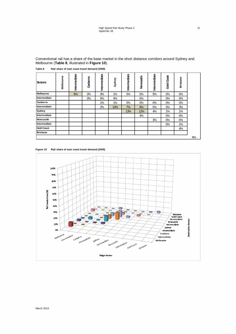
Conventional rail has a share of the base market in the short distance corridors around Sydney and Melbourne (Table 8, illustrated in Figure 10). Table 8 Rail share of east coast travel demand (2009)
Figure 10 Rail share of east coast travel demand (2009)
Sectors
Mel
bour
ne
Inte
rmed
iate
Canb
erra
Inte
rmed
iate
Sydn
ey
Inte
rmed
iate
New
cast
le
Inte
rmed
iate
Gol
d Co
ast
Bris
bane
Melbourne 8% 0% 3% 1% 0% 0% 5% 0% 0%Intermediate 0% 0% 4% 0% 0% 0%Canberra 1% 1% 0% 0% 0% 0% 0%Intermediate 2% 10% 7% 6% 0% 0% 3%Sydney 13% 12% 4% 1% 1%Intermediate 3% 0% 0%Newcastle 3% 0% 0%Intermediate 0% 1%Gold Coast 4%Brisbane
6%

High Speed Rail Study Phase 2 Appendix 1B
March 2013
11
Coach travel accounts for a small part of the base market in the corridor, its share being highest between Sydney and Canberra (Table 9 and Figure 11).
Table 9 Coach share of east coast travel demand (2009)
Figure 11 Coach share of east coast travel demand (2009)
Sectors
Mel
bour
ne
Inte
rmed
iate
Canb
erra
Inte
rmed
iate
Sydn
ey
Inte
rmed
iate
New
cast
le
Inte
rmed
iate
Gol
d Co
ast
Bris
bane
Tota
l
Melbourne 3% 1% 2% 0% 1% 1% 1% 1% 0%Intermediate 3% 6% 3% 2% 3% 1%Canberra 2% 10% 5% 2% 4% 2% 1%Intermediate 2% 3% 3% 3% 2% 3% 2%Sydney 2% 3% 4% 1% 0%Intermediate 3% 4% 1%Newcastle 2% 1% 2%Intermediate 2% 3%Gold Coast 2%Brisbane
Total 3%

High Speed Rail Study Phase 2 Appendix 1B
March 2013
12
5.0 Verification of the base market
5.1 Background Travel surveys involving contacting people at their homes can be subject to biases and uncertainties and it is a consequently accepted practice to compare the results of such surveys with independent travel demand data relating directly to the relevant transport modes. Typically, this would be counts of public transport passengers and road traffic.
In phase 1 of the study, independent passenger count data for air and rail travel in the corridor was available to validate these aspects of the base market data. This verification is repeated below for the new base market estimate.
Although base car travel demands were also compared with traffic counts on the main strategic highways, this was not an effective validation because the medium and long distance traffic which is the market for HSR could not be distinguished from other components of the traffic streams.
Regional diversion to HSR was predicted to be an important factor in phase 1 and much of this patronage was forecast to be diverted from car travel. Evidence from the household travel surveys used in developing metropolitan transport models also emphasises the particular risks of bias in car travel demand estimates from household surveys3.
For these reasons, a large scale number plate matching survey was commissioned between Melbourne and Sydney to provide independent data which could be used to validate the base car travel demand estimates derived from the NVS.
5.2 Verification against independent rail and air travel data Reliable independent information on current rail and air travel demands was obtained from CountryLink and BITRE, based on ticketing data. These sources are compared with the base demands in Table 10 and Table 11.
For the relatively small numbers of rail trips, the base travel market estimates match the CountryLink values.
Table 10 2009 Annual rail volumes by route
Route Phase 2 base market CountryLink Difference
percentage
Sydney-Melbourne 68,000 75,000 -9
Brisbane-Sydney 26,000 27,000 -4
Sydney-Canberra 53,000 55,000 -4
The base market estimates for non-transfer air passengers are lower than the total air passenger counts, partly because transfer passengers are included in the counts but are not represented in the base market estimates4. The proportion of transfers on some of the key domestic routes has been obtained from an airline ticketing data base (MIDT), as shown in Table 11. Together, the evidence from these independent data sources suggests that the base market estimates of non-transfer air passengers on these routes are reasonable, the exception being the two Gold Coast routes where the base market may underestimate the air demands.
3 Ashley et al, Recent information on the under-reporting of trips in household travel surveys, Australasian Transport Research Forum, 2009. 4 Trips to/from places outside the study area are not included in the base market estimates which includes air journeys outside the study area (including international) involving a connecting leg within the study area. Air journeys within the study area which involve a transfer are generally included in the base market, but have been excluded from the base market totals in the table.

High Speed Rail Study Phase 2 Appendix 1B
March 2013
13
Table 11 2009 Base air volumes by route (millions)
Route
Phase 2 base market (direct, non-transfer
trips)
Observed route passengers5
Difference Percentage (%)
Estimated transfer
percentage6
Sydney-Melbourne 5.5 7.1 -23 15
Brisbane-Sydney 3.3 4.3 -24 22
Brisbane-Melbourne 2.3 2.7 -14 9
Gold Coast-Sydney 1.4 2.1 -31 17
Gold Coast-Melbourne 1.1 1.6 -31 0
Canberra-Melbourne 0.9 1.1 -21 12
Sydney-Canberra 0.6 1.0 -45 36
5.3 Verification against independent car travel data: the registration number survey
5.3.1 The registration number survey
Because traffic counts alone could not provide a convincing verification of the NVS-based patterns of car travel in the corridor, a large-scale vehicle registration number survey was commissioned as part of this study (described in greater detail in Appendix 1C). The chosen location for the survey was the southern half of the corridor, between Sydney and Melbourne. Should significant biases be found in the NVS-based estimates of car travel, the required car travel demand adjustment factors would be assumed also to apply to the northern half of the corridor between Brisbane and Sydney.
The nature of the information sought and the scale of the survey, which may be unprecedented, imposed constraints on its design:
Some long distance car travel is likely to occur in part at night, implying the need for a 24 hour survey period.
Much of this travel is at the weekends (Appendix 3; Section 3.2), implying that the surveys should encompass Saturday and/or Sunday.
There was a need to survey a range of car journey lengths in case biases in the NVS data were a function of journey distance.
The very long distance journeys by car, especially those between Melbourne and Sydney, could be expected to be quite rare.
In order to meet these requirements, surveys were commissioned which used specialised video equipment that could capture number plates both during the day and at night, and target sample size requirements were developed based on the long distance travel demands in the highway corridor between Melbourne and Sydney derived from the NVS.
The survey was carried out by Austraffic and occurred over five days, for the full 24 hours, capturing northbound traffic along the Hume Highway. The survey locations (as indicated in Table 12 and Figure 12) were designed to estimate the six different light vehicle travel flows identified in Table 13, covering a range of travel distances.
The captured number plate data was later reviewed manually from the video footage and the number plate data was entered into a program which matched the number plates between the survey stations. Overall, 289,888 vehicles were observed and 95.4 per cent of plates were captured.
5 BITRE, Domestic Airline Activity Statistics, 2009. 6 Derived from the 2010 MIDT airline ticketing data base.

High Speed Rail Study Phase 2 Appendix 1B
March 2013
14
Table 12 Number plate survey locations
Site No. Description
1 North of Seymour
2 South of Wodonga
3 North of Albury
4 South of Yass
5 South of Goulburn
6 South of Campbelltown Figure 12 Survey locations
Table 13 Light vehicle flows surveyed
Targeted travel demand Centre to centre journey distance
Melbourne-Albury ~300 km
Melbourne-Canberra ~700 km
Melbourne-Sydney ~900 km
Albury-Canberra ~350 km
Albury-Sydney ~600 km
Canberra-Sydney ~300 km
#
#
# #
#
#
#
#
#
##
#
##
#
##
#
""
""""
""""
""
#
"
Road Typemotorwayprimarysecondarytrunk
Potential Stations
Survey Locations
Point
Point
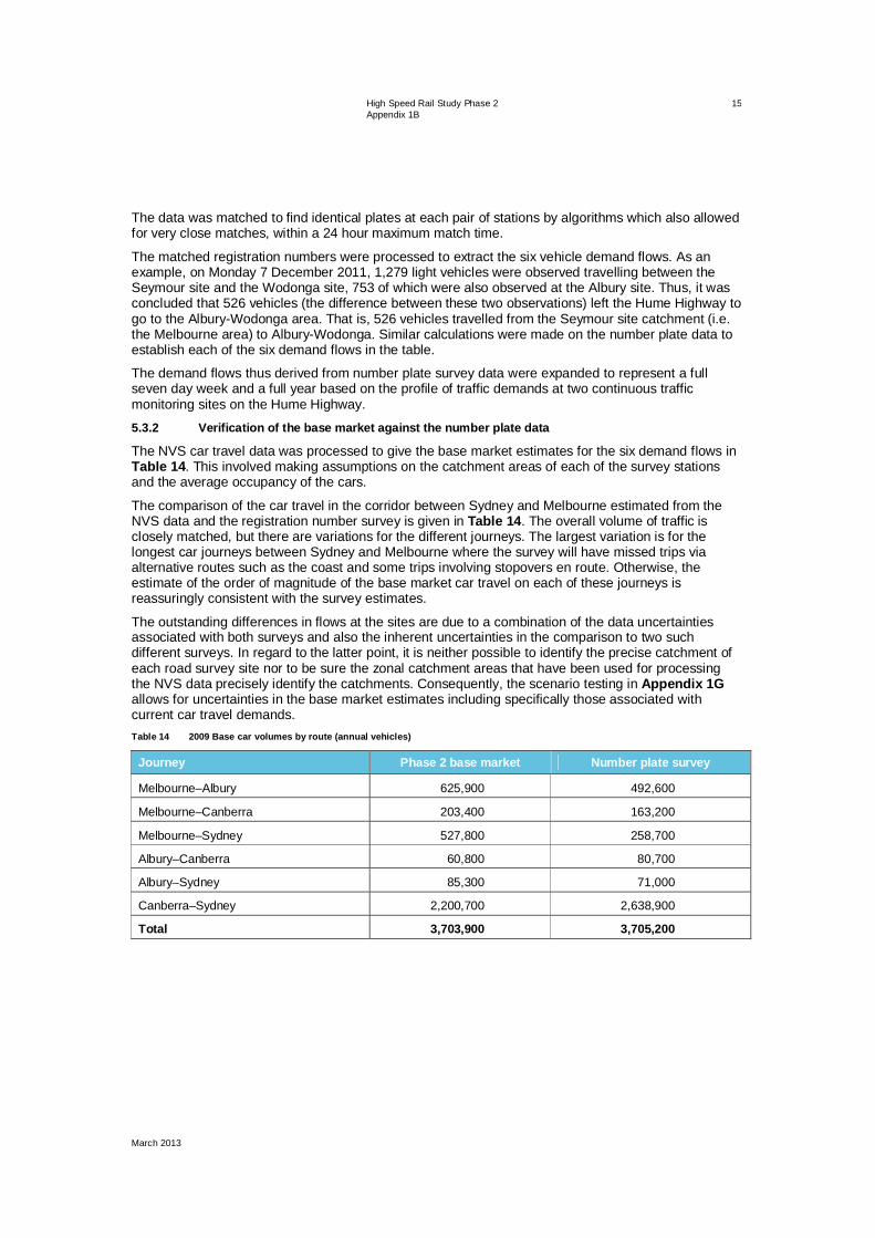
High Speed Rail Study Phase 2 Appendix 1B
March 2013
15
The data was matched to find identical plates at each pair of stations by algorithms which also allowed for very close matches, within a 24 hour maximum match time.
The matched registration numbers were processed to extract the six vehicle demand flows. As an example, on Monday 7 December 2011, 1,279 light vehicles were observed travelling between the Seymour site and the Wodonga site, 753 of which were also observed at the Albury site. Thus, it was concluded that 526 vehicles (the difference between these two observations) left the Hume Highway to go to the Albury-Wodonga area. That is, 526 vehicles travelled from the Seymour site catchment (i.e. the Melbourne area) to Albury-Wodonga. Similar calculations were made on the number plate data to establish each of the six demand flows in the table.
The demand flows thus derived from number plate survey data were expanded to represent a full seven day week and a full year based on the profile of traffic demands at two continuous traffic monitoring sites on the Hume Highway.
5.3.2 Verification of the base market against the number plate data
The NVS car travel data was processed to give the base market estimates for the six demand flows in Table 14. This involved making assumptions on the catchment areas of each of the survey stations and the average occupancy of the cars.
The comparison of the car travel in the corridor between Sydney and Melbourne estimated from the NVS data and the registration number survey is given in Table 14. The overall volume of traffic is closely matched, but there are variations for the different journeys. The largest variation is for the longest car journeys between Sydney and Melbourne where the survey will have missed trips via alternative routes such as the coast and some trips involving stopovers en route. Otherwise, the estimate of the order of magnitude of the base market car travel on each of these journeys is reassuringly consistent with the survey estimates.
The outstanding differences in flows at the sites are due to a combination of the data uncertainties associated with both surveys and also the inherent uncertainties in the comparison to two such different surveys. In regard to the latter point, it is neither possible to identify the precise catchment of each road survey site nor to be sure the zonal catchment areas that have been used for processing the NVS data precisely identify the catchments. Consequently, the scenario testing in Appendix 1G allows for uncertainties in the base market estimates including specifically those associated with current car travel demands. Table 14 2009 Base car volumes by route (annual vehicles)
Journey Phase 2 base market Number plate survey
Melbourne–Albury 625,900 492,600
Melbourne–Canberra 203,400 163,200
Melbourne–Sydney 527,800 258,700
Albury–Canberra 60,800 80,700
Albury–Sydney 85,300 71,000
Canberra–Sydney 2,200,700 2,638,900
Total 3,703,900 3,705,200

High Speed Rail Study Phase 2 Appendix 1B
March 2013
16
5.4 Distributions of travel origins and destinations between CBDs and suburban areas in major metropolitan areas
The distributions of travel demand within the metropolitan areas in the base matrices are illustrated in Figure 13 to Figure 18 separately for residents of each city and visitors to each city. In all three cities, residents’ trip origins and destinations are spread around the metropolitan areas, whereas there is a concentration of visitor trips in the city CBD.
Figure 13 Distribution of Sydney residents’ trips in the base matrix

High Speed Rail Study Phase 2 Appendix 1B
March 2013
17
Figure 14 Distribution of Sydney visitors’ trips in the base matrix
Figure 15 Distribution of Melbourne residents’ trips in the base matrix
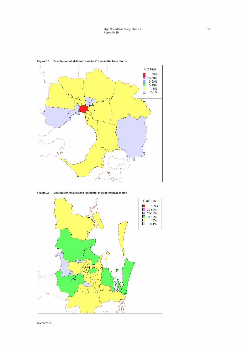
High Speed Rail Study Phase 2 Appendix 1B
March 2013
18
Figure 16 Distribution of Melbourne visitors’ trips in the base matrix
Figure 17 Distribution of Brisbane residents’ trips in the base matrix

High Speed Rail Study Phase 2 Appendix 1B
March 2013
19
Figure 18 Distribution of Brisbane visitors’ trips in the base matrix
The balance of metropolitan journeys between the CBD and outer areas is an important factor in determining the market for HSR. There is some available information on the distributions of the ground origins of trips to and from Brisbane and Sydney Airports which has been compared with the NVS data.
The distribution of the ground origins of all trips to and from Brisbane Airport is published in the Brisbane Airport 2009 Master Plan7. This does not distinguish residents from visitors and also encompasses international air passenger trips and other non-air passenger trips (such as the commuting of airport workers). This indicates that 47 per cent of trips are to/from the inner area of Brisbane. The equivalent figures for domestic air passengers in the east coast corridor from the phase 2 base matrices are 42 per cent. Thus, although these two data sources are not consistent in scope, the overall proportion of NVS base market trips generated in the inner and CBD areas of Brisbane is not incompatible with the airport data.
Similar information for Sydney airport is available from a 2006 survey of airport users, which Sydney Airport Corporation (SACL) has given approval to use. The earlier Speedrail surveys also provide additional data on both air and car travel in the Sydney-Canberra corridor (Table 15)8. Again, these data sources are not fully consistent in scope with the NVS base matrix, but the comparisons do not suggest that there is any bias in the proportion of trips starting or ending in central Sydney in the phase 2 base matrices.
7 Brisbane Airport Corporation, Brisbane Airport 2009 Master Plan, 2009. 8 SKM & MVA, Speedrail Patronage and Revenue Forecasts, Supplementary to final report, 1999.

High Speed Rail Study Phase 2 Appendix 1B
March 2013
20
Table 15 2009 Proportion of journeys beginning and ending in central Sydney: the phase 2 base matrices compared with Speedrail
data and SACL air passenger surveys
Segment Phase 2 2009 base matrices
Speedrail 1997/8 base matrices9
SACL 2006 Domestic air passenger
surveys10
Car travel
Business 42% 41% -
Other 34% 36% -
Air travel
Business 63% 68% 49%
Other 53% 62% 53%
6.0 Verification conclusions While there are individual differences, the verification exercises have demonstrated a strong overall consistency between the phase 2 base matrices and the independent data sources covering rail, air and car travel demands in the corridor.
9 The Speedrail data is for travel in the Sydney-Canberra corridor. 10 The SACL data is for all domestic air travel at Sydney Airport.

High Speed Rail Study Phase 2
Department of Infrastructure and Transport March 2013
Appendix 1C Number plate survey

High Speed Rail Study Phase 2 Appendix 1C
March 2013
Appendix 1C Number plate survey
Prepared for
Department of Infrastructure and Transport
Prepared by AECOM Australia Pty Ltd Level 21, 420 George Street, Sydney NSW 2000, PO Box Q410, QVB Post Office NSW 1230, Australia T +61 2 8934 0000 F +61 2 8934 0001 www.aecom.com ABN 20 093 846 925
March 2013
AECOM in Australia and New Zealand is certified to the latest version of ISO9001 and ISO14001.
© AECOM Australia Pty Ltd (AECOM). All rights reserved.
In accordance with the east coast high speed rail (HSR) study terms of reference, AECOM and its sub-consultants (Grimshaw, KPMG, SKM, ACIL Tasman, Booz & Co and Hyder, hereafter referred to collectively as the Study Team) have prepared this report (Report). The Study Team has prepared this Report for the sole use of the Commonwealth Government: Department of Infrastructure and Transport (Client) and for a specific purpose, each as expressly stated in the Report. No other party should rely on this Report or the information contain in it without the prior written consent of the Study Team. The Study Team undertakes no duty, nor accepts any responsibility or liability, to any third party who may rely upon or use this Report. The Study Team has prepared this Report based on the Client's description of its requirements, exercising the degree of skill, care and diligence expected of a consultant performing the same or similar services for the same or similar study, and having regard to assumptions that the Study Team can reasonably be expected to make in accordance with sound professional principles. The Study Team may also have relied upon information provided by the Client and other third parties to prepare this Report, some of which may not have been verified or checked for accuracy, adequacy or completeness. The Report must not be modified or adapted in any way and may be transmitted, reproduced or disseminated only in its entirety. Any third party that receives this Report, by their acceptance or use of it, releases the Study Team and its related entities from any liability for direct, indirect, consequential or special loss or damage whether arising in contract, warranty, express or implied, tort or otherwise, and irrespective of fault, negligence and strict liability. The projections, estimation of capital and operational costs, assumptions, methodologies and other information in this Report have been developed by the Study Team from its independent research effort, general knowledge of the industry and consultations with various third parties (Information Providers) to produce the Report and arrive at its conclusions. The Study Team has not verified information provided by the Information Providers (unless specifically noted otherwise) and it assumes no responsibility nor makes any representations with respect to the adequacy, accuracy or completeness of such information. No responsibility is assumed for inaccuracies in reporting by Information Providers including, without limitation, inaccuracies in any other data source whether provided in writing or orally used in preparing or presenting the Report. In addition, the Report is based upon information that was obtained on or before the date in which the Report was prepared. Circumstances and events may occur following the date on which such information was obtained that are beyond the Study Team's control and which may affect the findings or projections contained in the Report, including but not limited to changes in 'external' factors such as changes in government policy; changes in law; fluctuations in market conditions, needs and behaviour; the pricing of carbon, fuel, products, materials, equipment, services and labour; financing options; alternate modes of transport or construction of other means of transport; population growth or decline; or changes in the Client's needs and requirements affecting the development of the project. The Study Team may not be held responsible or liable for such circumstances or events and specifically disclaim any responsibility therefore.

High Speed Rail Study Phase 2 Appendix 1C
March 2013
Quality information Document Appendix 1C
Ref 60238250-1.0-REP-0101–1C
Date March 2013

High Speed Rail Study Phase 2 Appendix 1C
March 2013
Table of contents 1.0 Introduction and objectives 1 2.0 Survey background 1 3.0 Methodology 1 4.0 Analysis 2 5.0 Detailed results 4

High Speed Rail Study Phase 2 Appendix 1C
March 2013
1
1.0 Introduction and objectives Because traffic counts alone could not provide a convincing verification of the National Visitor Survey (NVS)-based patterns of current car travel in the corridor, a large-scale vehicle registration number survey was commissioned as part of this study. The chosen location for the survey was the southern half of the corridor, between Sydney and Melbourne.
The nature of the information sought and the scale of the survey, which may be unprecedented, imposed constraints on its design:
Some long distance car travel is likely to occur in part at night, which implied the need for a 24 hour survey period.
Much of this travel occurs at the weekends, which implied that the surveys should encompass Saturdays and/or Sundays.
There was a need to survey a range of car journey lengths in case biases in the NVS data were a function of journey distance.
The very long distance journeys by car, especially those between Melbourne and Sydney, were expected to be quite rare.
2.0 Survey background The number plate survey was designed to estimate the number of car journeys between the survey locations – broadly, Melbourne, Albury-Wodonga, Canberra and Sydney. Austraffic was commissioned to conduct the survey of vehicles on the Hume Freeway/Highway. While the scope of the study was light vehicles, this was extended for the Federal Department of Infrastructure and Transport to include Heavy Vehicles. The survey was conducted in the north-easterly direction.
3.0 Methodology Austraffic has a proven methodology for conducting Origin/Destination (OD) video surveys. Video surveys use specialised video equipment that captures vision of number plates during the day and night. For this study, the survey comprised the following survey sites in Table 1. Table 1 Number plate survey locations
Site no. Description (all north-east-bound on Hume Freeway)
1 North of Seymour, just west of Seymour-Avenel Rd
2 South of Wodonga, east of Indigo Creek Rd
3 North of Albury, north of Ettamogah Rd
4 South of Yass, north of on-ramp to Yass Valley Way
5 South of Goulburn, south of Drews Rd
6 South of Campbelltown, between Menangle Rd and Narellan Rd
The Hume Highway video survey was installed on 5 and 6 December 2011. An onsite job safety analysis was conducted in line with Austraffic’s business management system. The sites were positioned with regard to safety considerations and the need to find appropriate roadside poles to secure the equipment to that were not located beyond the next nearest intersection. All video sites were checked prior to actual commencement of the survey period to ensure the video was in focus and recording correctly. The video equipment was synchronised to ensure accuracy of data. All survey equipment was checked regularly for about 16 hours each day. Batteries and recording drives/cards were replaced daily. On completion of the survey on 12 December 2011, the video equipment was collected.

High Speed Rail Study Phase 2 Appendix 1C
March 2013
2
The survey was designed to capture number plates over five days from Wednesday 7 December - Sunday 11 December 2011 inclusive. Extra video was captured at stations 2-6 on the morning of Monday 12 December 2011 to allow plates captured before midnight on Sunday to be matched along the Hume Freeway/Highway.
The captured data was later reviewed manually from the video footage, allowing staff to pause each vehicle as it passed, ensuring highly accurate number plate readings and vehicle classification. Number plate data was entered into the Austraffic Origin-Destination (OD) software program, which matches the number plates between the survey stations.
While the video technology allowed the capture of the majority of number plates, a small percentage of plates were not accurately visible due to:
Dirty, obscured or missing plates, or cars travelling very close together.
Direct sunlight – at some times during daylight hours some cameras were subject to sunlight shining directly onto the front of the lens, causing glare which severely restricted the ability to read the number plates during these periods. Given the constraints on positioning the cameras due to considerations of safety, optimum results and road conditions, brief intervals of sun glare were unavoidable in some locations.
Motorcycles – due to the orientation of the cameras facing oncoming traffic, motorcycles, which are not required to display front number plates, were not recorded.
A major vandalism incident occurred at most stations on the night of Saturday 10 December. All video equipment at stations 1-5 was badly damaged and thrown into nearby grasslands, and hard drives and other equipment was stolen. The damage was reported to each local police station. The vandalism resulted in a loss of data at these five stations for all of Saturday night and at stations 2 and 3 on Friday night (as the hard drives had not been replaced on Saturday). Austraffic made every effort to reinstate all the survey stations with spare equipment. This occurred progressively on Sunday morning and for the remainder of the survey data collection continued. The actions performed by Austraffic during the analysis to take into account these data outages are described in the next section.
4.0 Analysis From the video footage, number plates, vehicle type and time were recorded for each vehicle at each site. The vehicle classes reported were:
Cars and light commercial vehicles.
Trucks and buses.
While Austraffic attempted to record all vehicle number plates at each survey site, technical issues occasionally prevented viewing of all number plates. The total passing traffic volumes were recorded and the percentage of missed plates reported. The number of missed plates for each site is shown in Table 2. For the hours when the vandalism occurred, Austraffic estimated missing traffic volumes and number plates in line with trends for that site. Overall, 289,888 vehicles were observed and 95.4 per cent of plates were captured.

High Speed Rail Study Phase 2 Appendix 1C
March 2013
3
Table 2 Captured plates report
Site Total count Plates captured Capture rate
1 27,083 26,459 97.7%
2 29,732 29,073 97.8%
3 24,037 23,293 96.9%
4 33,588 30,737 91.5%
5 58,794 57,019 97.0%
6 116,654 109,948 94.3%
Total 289,888 276,529 95.4%
All number plate data was entered into Austraffic’s OD computer software analysis suite. The data was matched to find identical plates from one site to the next. The data matching was also refined to allow for very close matches where the characters may have been the same (e.g. ‘O’, ‘Q’ and ‘0’) or have only been partially recorded due to impaired visibility of the number plate. A ‘wildcard’ character was used in data entry and processing where the entire plate could not be recorded accurately. Misclassified vehicles with the same plate were corrected.
After reviewing the matched data, the trip tables were produced using an agreed match time for through traffic trips. A 24 hour maximum match time was used to define continuous trips between all of the stations. Trips which took longer than 24 hours were not considered.
On the Saturday night of the surveys, vandalism caused video outages at sites 1-5 and all vision during the night time hours was lost. Video was also lost on Friday night at sites 2 and 3 from the same incident. To account for these video outages, Austraffic adjusted the traffic volumes and match rates during those times based on the traffic volumes/match rates before and after that time of day and from other days for the same sites.
Where missed plates occurred either through vandalism or poor visibility, the trip tables were adjusted in line with trends for that site over the day so that the trip tables reflect the total passing traffic volumes.
The issues involved with factoring for missed number plates are complex. Austraffic analyses the data cell by cell and hour by hour. The missed plates factor takes into account the percentage for each site, within each cell, within each hour of the trip tables. Austraffic uses a factor based on probability to increase the through traffic to compensate for missed plates. The factor is the inverse of the captured plate’s percentage for the inbound site, multiplied by the captured plate’s percentage for the outbound site.
Austraffic allowed for survey ‘shutdown errors’ where the survey ended before inbound trips had time to complete their journey. While the survey ceased at midnight on the Sunday at site 1 near Seymour, the video recording was extended for a number of hours at each site further to the north. The last site near Campbelltown continued recording until 1pm on the Monday. Therefore, adequate time was allowed for vehicles to be captured at subsequent sites further along the freeway.

High Speed Rail Study Phase 2 Appendix 1C
March 2013
4
5.0 Detailed results Detailed results are available from the survey for light vehicles only, heavy vehicles only or all vehicles, as illustrated by the following examples. Table 3 shows the total number of matched number plates at each pair of survey sites over the five days of surveys and the total traffic volumes (light vehicles) at each survey site. As an example, site 1E is at Seymour, where 20,364 light vehicles were observed passing the site during the survey period. Of these, according to the registration number matching, 8,399 vehicles were also observed at site 2N (Wodonga) and 1,868 at site 6N (Campbelltown). Table 3 Overall results matrix (light vehicles): the matched registration numbers at each pair of sites
OD Matrix Destination 2N 3N 4E 5N 6N
Origin Recorded 22,271 17,640 24,211 46,019 89,742
1E 20,364 8,399 4,896 3,616 2,492 1,868
2N 22,271 5,962 4,287 3,081 2,394
3N 17,640 5,501 3,756 2,896
4E 24,211 9,418 6,289
5N 46,019 25,269
The matching data is available for each hour of each day of the survey. For example, in Figure 1, which relates to the Seymour and Wodonga sites (sites 1E and 2N), the hourly light vehicle traffic volumes at each site over the survey period are given, together with the number of matched numberplates of vehicles travelling between these two sites.
Figure 2 and Figure 3 show the matches for successively longer journeys, from Seymour to Yass and Campbelltown respectively. The matches reduce as a proportion of the traffic flow as the distance increases, corresponding with the lower frequency of the longer journeys. The much higher traffic volumes at Campbelltown en route to Sydney are also apparent. Figure 1 Hourly traffic volumes at sites 1E (Seymour) and 2N (Wodonga), and the counts of matched number plates
0
100
200
300
400
500
600
0 6 12 18 0 6 12 18 0 6 12 18 0 6 12 18 0 6 12 18
Vehi
cles
Time Starting
Origin
Destination
Matches

High Speed Rail Study Phase 2 Appendix 1C
March 2013
5
Figure 2 Hourly traffic volumes at sites 1E (Seymour) and 4E (Yass), and the counts of matched number plates
Figure 3 Hourly traffic volumes at sites 1E (Seymour) and 6N (Campbelltown), and the counts of matched number plates
0
100
200
300
400
500
600
700
800
0 6 12 18 0 6 12 18 0 6 12 18 0 6 12 18 0 6 12 18
Vehi
cles
Time Starting
Origin
Destination
Matches
0
500
1000
1500
2000
2500
0 6 12 18 0 6 12 18 0 6 12 18 0 6 12 18 0 6 12 18
Vehi
cles
Time Starting
Origin
Destination
Matches

High Speed Rail Study Phase 2 Appendix 1C
March 2013
6
By recording the time at which each registration number is observed, information on the time taken by each vehicle to travel between each pair of sites is obtained. Figure 4 to Figure 6 illustrate the distributions of journey times in 15 minute bands for journeys from Seymour to Wodonga, Yass and Campbelltown respectively.
For the shortest journey, between Seymour and Wodonga, most vehicles take between 1 hour 30 minutes and 2 hours 15 minutes. As the journey time increases, a greater spread of journey times is also apparent. Figure 4 The distribution of travel times between sites 1E (Seymour) and 2N (Wodonga)
Figure 5 The distribution of travel times between sites 1E (Seymour) and 4E (Yass)
0%
5%
10%
15%
20%
25%
30%
35%
40%
45%
0 1 2 3 4 5 6 7 8 9 10 11 12 13 14 15 16 17 18 19 20 21 22 23
Perc
enta
ge o
f veh
icle
s
Travel time (hours)
0%
2%
4%
6%
8%
10%
12%
14%
0 1 2 3 4 5 6 7 8 9 10 11 12 13 14 15 16 17 18 19 20 21 22 23
Perc
enta
ge o
f veh
icle
s
Travel time (hours)

High Speed Rail Study Phase 2 Appendix 1C
March 2013
7
Figure 6 The distribution of travel times between sites 1E (Seymour) and 6N (Campbelltown)
From the same travel time data, information is available on the variations in the average and median journey times between each pair of sites by hour of the day and day of the survey. Figure 7 to Figure 9 provides this information for the same three journeys (Seymour to Wodonga, Yass and Campbelltown respectively). It is apparent from these figures that not only does the variation in travel time increase as journey distance increases but, for the longer trips, it also varies markedly by time of day.
Figure 7 Average and median travel times through the survey period for journeys from site 1E (Seymour) to site 2N (Wodonga)
0%
1%
2%
3%
4%
5%
6%
7%
8%
9%
10%
0 1 2 3 4 5 6 7 8 9 10 11 12 13 14 15 16 17 18 19 20 21 22 23
Perc
enta
ge o
f veh
icle
s
Travel time (hours)
0123456789
101112131415161718192021222324
0 6 12 18 0 6 12 18 0 6 12 18 0 6 12 18 0 6 12 18
Trav
le ti
me
(hou
rs)
Start time
Average Travel Time
Median Travel Time

High Speed Rail Study Phase 2 Appendix 1C
March 2013
8
Figure 8 Average and median travel times through the survey period for journeys from site 1E (Seymour) to site 4E (Yass)
Figure 9 Average and median travel times through the survey period for journeys from site 1E (Seymour) to site 6N (Campbelltown)
0123456789
101112131415161718192021222324
0 6 12 18 0 6 12 18 0 6 12 18 0 6 12 18 0 6 12 18
Trav
le ti
me
(hou
rs)
Start time
Average Travel Time
Median Travel Time
0123456789
101112131415161718192021222324
0 6 12 18 0 6 12 18 0 6 12 18 0 6 12 18 0 6 12 18
Trav
le ti
me
(hou
rs)
Start time
Average Travel Time
Median Travel Time

High Speed Rail Study Phase 2
Department of Infrastructure and Transport March 2013
Appendix 1D Stated preference survey
High Speed Rail Study Phase 2 Appendix 1D
March 2013
Appendix 1D Stated preference survey
Prepared for
Department of Infrastructure and Transport
Prepared by AECOM Australia Pty Ltd Level 21, 420 George Street, Sydney NSW 2000, PO Box Q410, QVB Post Office NSW 1230, Australia T +61 2 8934 0000 F +61 2 8934 0001 www.aecom.com ABN 20 093 846 925
March 2013
AECOM in Australia and New Zealand is certified to the latest version of ISO9001 and ISO14001.
© AECOM Australia Pty Ltd (AECOM). All rights reserved.
In accordance with the east coast high speed rail (HSR) study terms of reference, AECOM and its sub-consultants (Grimshaw, KPMG, SKM, ACIL Tasman, Booz & Co and Hyder, hereafter referred to collectively as the Study Team) have prepared this report (Report). The Study Team has prepared this Report for the sole use of the Commonwealth Government: Department of Infrastructure and Transport (Client) and for a specific purpose, each as expressly stated in the Report. No other party should rely on this Report or the information contain in it without the prior written consent of the Study Team. The Study Team undertakes no duty, nor accepts any responsibility or liability, to any third party who may rely upon or use this Report. The Study Team has prepared this Report based on the Client's description of its requirements, exercising the degree of skill, care and diligence expected of a consultant performing the same or similar services for the same or similar study, and having regard to assumptions that the Study Team can reasonably be expected to make in accordance with sound professional principles. The Study Team may also have relied upon information provided by the Client and other third parties to prepare this Report, some of which may not have been verified or checked for accuracy, adequacy or completeness. The Report must not be modified or adapted in any way and may be transmitted, reproduced or disseminated only in its entirety. Any third party that receives this Report, by their acceptance or use of it, releases the Study Team and its related entities from any liability for direct, indirect, consequential or special loss or damage whether arising in contract, warranty, express or implied, tort or otherwise, and irrespective of fault, negligence and strict liability. The projections, estimation of capital and operational costs, assumptions, methodologies and other information in this Report have been developed by the Study Team from its independent research effort, general knowledge of the industry and consultations with various third parties (Information Providers) to produce the Report and arrive at its conclusions. The Study Team has not verified information provided by the Information Providers (unless specifically noted otherwise) and it assumes no responsibility nor makes any representations with respect to the adequacy, accuracy or completeness of such information. No responsibility is assumed for inaccuracies in reporting by Information Providers including, without limitation, inaccuracies in any other data source whether provided in writing or orally used in preparing or presenting the Report. In addition, the Report is based upon information that was obtained on or before the date in which the Report was prepared. Circumstances and events may occur following the date on which such information was obtained that are beyond the Study Team's control and which may affect the findings or projections contained in the Report, including but not limited to changes in 'external' factors such as changes in government policy; changes in law; fluctuations in market conditions, needs and behaviour; the pricing of carbon, fuel, products, materials, equipment, services and labour; financing options; alternate modes of transport or construction of other means of transport; population growth or decline; or changes in the Client's needs and requirements affecting the development of the project. The Study Team may not be held responsible or liable for such circumstances or events and specifically disclaim any responsibility therefore.

High Speed Rail Study Phase 2 Appendix 1D
March 2013
Quality information Document Appendix 1D
Ref 60238250-1.0-REP-0101–1D
Date March 2013

High Speed Rail Study Phase 2 Appendix 1D
March 2013
Table of contents 1.0 Introduction and objectives 1 2.0 Development of designs and format 1
2.1 Chosen movements and modes 1 2.2 Presentation and design of the stated preference experiments 3 2.3 Questionnaire development and implementation 6 2.4 Piloting and sampling 6
3.0 Main survey 8 3.1 Dates and numbers 8 3.2 Data cleaning process 9 3.3 Sample demographics 9 3.4 Overall sample characteristics 11 3.5 Characteristics of the revealed preference mode choices 13 3.6 HSR station access 15 3.7 HSR choices 18
4.0 Main survey – analysis of SP data 19 4.1 Analysis of station choice SP 20 4.2 Analysis of mode choice SP data (all modes) 24 4.3 Combined estimation 32
5.0 Recommendation on coefficients and implementation for demand model 36 5.1 Scaling parameters 37 5.2 Modal hierarchy 39 5.3 Generalised cost weights 39 5.4 Values of time and ASCs 40 5.5 Calibration to revealed preference data 45
6.0 Conclusions 52

High Speed Rail Study Phase 2 Appendix 1D
March 2013
1
1.0 Introduction and objectives The phase 1 demand model parameter values were based on a distillation of local and international experience. In recognition of the importance of demonstrating that these parameter values are representative of local travel choice behaviour and the demand forecasts appropriately sensitive to the attributes of the high speed rail (HSR) service, a stated preference (SP) survey of the choice of travel mode was carried out in the east coast corridor.
The objectives of the survey were to investigate the key demand model parameters:
The scaling parameters, which determine the overall sensitivity of the shares for each transport mode to changes in transport accessibility.
The time values of medium and long distance travellers, which determine how sensitive mode shares are to transport prices.
The choice of station and mode of station access.
The extent of preference (or otherwise) for HSR over-and-above the measurable improvements in level-of-service (journeys times, service frequencies, fares, access and egress), referred to as the HSR alternative specific constant (ASC).
Because many of these issues relate to the HSR service and its attractiveness in comparison with current modes of transport, information on current transport choices (referred to as revealed preference) would be of limited usefulness. It is in such circumstances that SP survey techniques are appropriate.
Where evidence of travel choice behaviour cannot be obtained in real life, for example where a new transport mode such as HSR is being considered, SP survey techniques provide a means of exploring how people making relevant journeys would react to the introduction of such a mode.
This survey followed international practice, in that people making relevant journeys within the east coast study area were identified and presented with hypothetical scenarios in which an HSR service would provide for their journey, and asked to choose between their existing transport mode and HSR. Each survey respondent was presented with nine different scenarios in each of which the competitive position of HSR relative to their current mode was varied.
Statistical analysis of the data on travel choices obtained from SP surveys then provides considerable information on how people weigh up the different aspects of each transport mode in choosing between the alternatives.
The survey was informed by focus group discussions and a pilot survey. The survey began with a recruitment interview involving initial telephone contact to identify people who had made relevant journeys and were willing to participate in the survey. Specific journey information was obtained which was incorporated into a subsequent SP interview.
2.0 Development of designs and format
2.1 Chosen movements and modes On the grounds of survey efficiency, it was decided to restrict the number of home (‘production’) areas that would be surveyed to six cities/towns as shown in Table 1. This includes two major cities (Melbourne and Sydney), two large population centres (Canberra and Newcastle) and two regional towns (Albury-Wodonga and Wagga Wagga). With the emphasis on longer distance travel, behaviour is expected to be transferable between locations.
For each of these areas, the likely demand to other areas was investigated using the National Visitor Survey (NVS)-based travel demand market information (see Appendix 1B for more detail), having regard to the modes used, separately for business and leisure purposes. Origin/destination (OD) movements to destinations which were considered unlikely to be part of the potential HSR market were ignored, being either too short or too long (e.g. Brisbane-Melbourne), or having too little demand.

High Speed Rail Study Phase 2 Appendix 1D
March 2013
2
In addition, it was decided that, for any OD cell, modes with a share less than 20 per cent would be excluded, though an exception was made for Newcastle-Sydney in order that current rail users could be included in the sample. This again was on the grounds of survey efficiency.
On this basis, the set of chosen movements and modes was as illustrated in Table 1, which also indicates those chosen for the pilot. Table 1 Sample movements
Home location Destinations Modes for business
Modes for non-business Included in pilot
Melbourne
Albury Car Car Yes
Shepparton1 Car Car Yes
Canberra Air Car and air Yes
Sydney Air Car and air Yes
Albury-Wodonga
Melbourne Car Car Yes
Canberra Car Car Yes
Sydney Car and air Car and air Yes
Wagga Wagga Canberra Car Car No
Sydney Car Car No
Canberra
Melbourne Air Car and air No
Albury Car Car No
Wagga Wagga Car Car No
Sydney Car and air Car No
Newcastle Air Car No
Sydney
Melbourne Air Car and air No
Albury Car and air Car No
Wagga Wagga Car and air Car No
Canberra Car and air Car No
Newcastle Car Car No
Port Macquarie Car and air Car No
Gold Coast Air Car and air No
Brisbane Air Car and air No
Newcastle
Canberra Car and air Car No
Sydney Car and rail Car and rail No
Brisbane Air Car and air No
Interview quotas were then defined according to four dimensions: home area, purpose, journey length, and mode. The base travel demand market was used to provide guidance as to whether the quotas were realistic and to ensure that the survey budget was not unnecessarily spent chasing observations for movements with very small demand. The quotas were designed to support an efficient process of reaching the target of 2000 respondents.
1 Shepparton was removed after the pilot as respondents did not vary their choice of mode in the SP.
High Speed Rail Study Phase 2 Appendix 1D
March 2013
3
Minimum quotas were only set on collections of cells (e.g. total business travellers from each origin), and in order to ensure that some sample was collected for smaller movements, a maximum quota was set for specific cells that were expected to be easily sampled (such as Melbourne-Sydney business travel by air).
In summary, the quotas were:
Melbourne = 500.
Albury-Wodonga = 150.
Wagga Wagga = 150.
Canberra = 250.
Sydney = 650.
Newcastle = 300.
Overall business sample 500.
Overall air sample 900.
Overall rail sample 50.
Regional destination (Albury-Wodonga, Wagga Wagga, Port Macquarie and Gold Coast) 200.
2.2 Presentation and design of the stated preference experiments It was decided to link two separate SP questions – on station choice and mode choice – using a simplified version of the experiment previously undertaken successfully for Speedrail2. The form of the experiment is set out in Figure 1 to Figure 3. The sequence of the interview is as follows.
Prior to the SP questions, each respondent is asked to choose their preferred mode of access to each of the station options (CBD, airport and Craigieburn in the example).
The respondent is then offered different travel contexts (‘scenarios’) to consider, in which the characteristics of their access to the stations, their journeys by HSR and their existing mode of transport are changed.
For each such context, the station choice SP offers station options detailing travel to the station for each option, based on the respondent’s reported modal preferences (these are in the form of ‘cards’, Figure 1).
The respondent expresses a preferred station (in this case, the CBD station) and, in the mode choice SP which immediately follows, is offered more details on the HSR journey to compare with a journey by their current mode of transport (either air, car or rail depending on the context of their journey). The SP questions for car and air are illustrated in Figure 2 and Figure 3 respectively.
This process is repeated for each of the travel scenarios.
2 SKM, Speedrail, Technical Note TN15:Stated Preference Experiment Fieldwork, 1999.

High Speed Rail Study Phase 2 Appendix 1D
March 2013
4
Figure 1 Example of station choice SP card
Figure 2 Example of mode choice SP card (HSR vs. car)

High Speed Rail Study Phase 2 Appendix 1D
March 2013
5
Figure 3 Example of mode choice SP card (HSR vs. air)
Note that two forms of presentation were possible, according to whether the respondent elected to receive a printed version by post or a web-based version. In both cases, however, the SP was customised to previously obtained travel data, and in both cases the main interviews were conducted by telephone. Therefore the distinction between the two forms of presentation was merely a matter of convenience for the respondent as to how they wanted to view the SP.
The basis of the SP approach is to present a sequence of choices (the scenarios) in which the variables relating to each alternative are varied in a systematic way. The plan which underlies this variation is referred to as the ‘design’. In developing the design, it is also necessary to decide how many scenarios should be offered to each respondent.
Separate designs were required for a) station choice, b) HSR vs. air mode choice, c) HSR vs. car mode choice and d) HSR vs. rail mode choice. In each case, the layout involved a set of blocks of nine scenarios, using an orthogonal design, with most variables at three levels3. It was found possible to use the same design for the different purposes and OD pairs, though some variations in the choice of values for levels were necessary.
A simulation testing process was set up separately for the four designs, with sufficient flexibility to be able to apply to different purposes and OD pairs. The simulation involved making assumptions about the generalised cost parameters (based primarily on the phase 1 model) together with some reasonable level of variation around these, and allowing for further random effects.
The simulation process had three primary aims: to investigate the likely level of ‘trading’ (a given respondent is considered to trade if he/she does not always choose the same alternative whatever the scenarios presented); to ensure that, given the simulated responses, the input coefficients could be
3 That is, in the design, three alternative values of the variable are offered to each respondent, and the variations for each attribute are independent of the variations for the other attributes (an orthogonal experimental design).

High Speed Rail Study Phase 2 Appendix 1D
March 2013
6
adequately recovered by estimation; and to enable variations to the levels and the underlying design to be quickly tested.
The combinations of modes, purposes and OD pairs required for the pilot were given priority in the testing process. A target level (maximum) of 25 per cent non-trading respondents was set to ensure that an adequate sample of useable pilot data would be obtained, though it was not always possible to achieve this, particularly for short distance car travel where the access and egress costs associated with HSR made it very difficult to make HSR competitive.
Overall, however, it was considered that satisfactory designs for piloting could be achieved. An important feature of the design is that HSR times and costs were pivoted off existing mode times and costs (subject to some realism constraints). This meant that in some cases, to induce trading, lower values of HSR times and, in particular, fares might be offered than would be the case in practice. However, these values were still considered to be credible.
2.3 Questionnaire development and implementation The main part of the questionnaire development is largely intended to ensure the collection of the data required to provide a basis for ‘customising’ the SP. As noted, the interview was conducted in two parts. The initial recruitment interview starts with a screening section (including scope and willingness to participate), followed by a section which elicits the key data about the respondent’s existing travel. Following this, the main SP questionnaire can be prepared, with the SP itself either delivered by post or made available by the web. In both cases, the questions are interviewer-administered over the telephone, using computer-assisted telephone interviewing technology.
In addition to the SP data, the main survey collects information about alternative modes that might have been used, offering the possibility of a revealed preference (RP)4 estimation for the current journey. Finally, some general socio-economic questions are also asked, with a view to providing possible segmentation variables and confirming the representativeness of the sample.
The various routeing possibilities within the questionnaire were set out in a flow chart and thoroughly tested for consistency. A key feature of the approach was the need to link the initial recruitment questionnaire with the main SP questionnaire. This required careful testing.
A preliminary version of the questionnaire was tested through in-depth interviews with 16 respondents. As well as reactions to the general structure of the questionnaire and the SP questions, information was obtained as to possible reasons for not trading, the importance of a careful description of the access/egress arrangements, the need for a prepared set of answers to potential questions about HSR, and the willingness to use the web-based form of the SP. This information was taken into account for the final version of the pilot.
2.4 Piloting and sampling The survey company I-view purchased a set of telephone numbers from Sample Pages (also referred to as Electronic White Pages). These numbers were a random set of residential telephone numbers from the postcodes specified for the pilot in Melbourne and Albury. A target sample of 100 respondents was proposed for the pilot, which focused on recruiting respondents travelling to the destinations (as well as via the modes and for the purposes) shown in Table 1.
The overall pilot sample was 98 completed responses (after removing two which turned out to be incomplete). To give an indication of the effort required to collect this sample, contact was made with 1,505 persons (which required 5,909 phone calls due to unanswered phones calls, call backs and answering machines). Of the 1,505, 54 per cent refused5 to answer the survey and six per cent could not be understood. Of the remaining 602 who were in principle willing participants, 63 per cent did not fit the criteria and a further 13 per cent were not used as the quota had already been met. Hence,
4 In which estimation is based on actual choices of the respondent. 5 The recruitment survey starts with “Good morning/afternoon/evening my name is ......................., I am from the market research firm I-view. I am calling in relation to the Australian Government’s high speed rail study between Melbourne, Sydney, Canberra and Brisbane”. It is possible that some of the refusals were because respondents were not interested in HSR.

High Speed Rail Study Phase 2 Appendix 1D
March 2013
7
interviews were initiated with 147 people; however, 49 of these dropped out between the recruitment and follow-up survey.
Of the 98 completed surveys, 77 were conducted using a web link and 21 by posting hardcopy cards.
The recruitment interview typically took 10 minutes and the follow-up interview, which included the SP cards, took 15 to 20 minutes.
Interviewers were requested to note down any feedback from the respondents, any trends they detected in the way people responded, and to enquire as to how easy respondents found the task and whether they felt that the choices offered to them were realistic. The feedback provided has been grouped into the following general themes:
Level of engagement
Despite being an onerous task with a lot of information to digest, most respondents stated that they were able to understand the task and that the scenarios offered were realistic. Although the interview took some time to complete, most people remained engaged due to the interest they showed in being asked about HSR.
In particular, Albury-Wodonga respondents were found to be much more willing to undertake the survey on first contact than those in Melbourne.
Support for HSR
A lot of comments were made about how respondents would like to see HSR built in Australia.
A number of people that did not choose HSR in any of the scenarios commented on closing that they would consider HSR for other journeys, but that it just did not suit this particular journey.
Potential improvements to SP
Respondents tended not to look at the time and cost implications of accessing different HSR stations, and SP response data strongly demonstrated that most had a clear preference as to which station was most convenient to their house. In fact, a lot of respondents found the station access choice a hindrance and wanted to proceed straight to the mode choice scenarios.
The numbers presented in the SP occasionally looked unrealistic.
The hard copy cards were difficult and needed to be improved. Many respondents were intimidated by having 18 different sheets of paper.
A lot of people did not want an incentive when it came to the end of the survey. They preferred not to give out personal details rather than receive a $10 gift card. But the incentive was felt to be worthwhile mentioning up front in order to attract interest.
Not many business trips were collected. Although a number of respondents were professionals, typically the last journey they had made (or the most memorable) was a leisure journey. It was felt that they could have been prompted to talk about a business journey instead.
The general characteristics of the pilot sample were considered to be a good representation of the wider population (of course, the population making long distance journeys will not necessarily be representative of the general population). A range of discrete choice models was estimated for different market segments using BIOGEME6. The results indicated that the desired coefficients could be recovered and, taking into account the small sample and the standard error of the estimated parameters, the key values were within expected bounds. Some parameters such as frequency and check-in time proved to be insignificant and changes were made to the survey to improve this.
6 M Bierlaire, BIOGEME: A free package for the estimation of discrete choice models, Proceedings of the 3rd Swiss Transportation Research Conference, Ascona, Switzerland, 2003.

High Speed Rail Study Phase 2 Appendix 1D
March 2013
8
Based on the interviewer feedback, independent reviews and the analysis of the data outputs, the following improvements and modifications were made:
The definition of ‘in scope’ respondents was tightened such that:
- People using frequent flyer points (or other free flights) were excluded.
- Non-home-based journeys must start within the home city.
- Air transit passengers were excluded.
- For air or rail journeys which were part of a multi-destination tour, the questionnaire was restricted to asking about the first leg of the tour only.
The categories for qualitative questions were refined based on the responses given in the pilot.
Refined wording was designed to ensure parking costs were captured in access/egress journeys.
The look of the of SP cards was improved to make them easier to understand.
Additional interviewer training was held to enable them to respond to a wider range of potential questions from respondents. This also included a matrix of approximate HSR travel times for the interviewer.
Frequency was made more prominent on the SP cards and is now shown alongside the total travel time and cost.
Upper and lower ranges were placed on values presented in the SP (and inputs values) to ensure more realistic trading (for example, an upper limit of two hours was set on flight times).
The $10 gift card offered as an incentive to respondents was retained but the respondent was given the option at the end of the survey to opt out of this if they did not wish to give out their address details.
3.0 Main survey
3.1 Dates and numbers Interviewers for the main survey were briefed on 5 March 2012 and commenced recruitment on 6 March 2012. A sample of 2,633 respondents had been recruited by 25 March 2012 and the required 2,000 follow-up surveys were completed by 4 April 2012, with some allowance for drop out between the two surveys.
The main survey focused on recruiting respondents from Melbourne, Sydney, Canberra, Newcastle, Wagga Wagga and Albury, travelling to the destinations (as well as via the modes and for the purposes) shown in Table 1.
To collect the sample, a total of 49,548 phone calls were made in order to speak with 31,120 people. Of those, 44 per cent refused to answer the survey, and eight per cent could not be understood. Of the remaining 13,447 who were in principle willing participants, 72 per cent did not fit the criteria and a further five per cent were not used as the quota had already been met. Hence, interviews were initiated with 3,024 people, but 1,024 of these (34 per cent) dropped out between the recruitment and follow-up survey.
With the exception of the number of calls required to make contact (which was especially high in the pilot at almost four calls per contact in comparison to 1.6 in the main survey), these figures demonstrate considerable consistency between the pilot and main survey. About 43 per cent of those contacted were willing to take part, but of those only 23 per cent were in scope. A third dropped out subsequently. The final sample was therefore only 6.4 per cent of those with whom contact was made.
The sample was derived from a random sample (Electronic White Pages) of telephone numbers.

High Speed Rail Study Phase 2 Appendix 1D
March 2013
9
The recruitment interview typically took 12 minutes and the follow-up interview, which included the SP cards, took 18 minutes. The respondent was encouraged to select the email version, as the pilot had shown this to be the easiest for the respondents to understand, and it was also easier for I-view to administer. As a result, the mail-out version was only required in 245 of the 2,000 cases.
As the number of changes made between the pilot and main survey was small, the two datasets were pooled for a final sample of 2,098 individual responses. Most quotas were met, with the exception of air and business travel, which were lower than expected. In both cases the possible shortfall was identified mid-way through the survey and interviewers were requested to ask for business and/or air trips first rather than asking for their most recent journey. Although this resulted in a slight increase in the proportion of business travel (20 per cent to 21.4 per cent, with a target of 25 per cent), there was no increase in the air travel sample.
3.2 Data cleaning process The data was put through a thorough process to check for erroneous entries. The result of this process was the removal of 37 respondents from the SP sample and a further eight from the RP sample potentially available for RP analysis (see Section 2.3). The reasons for their omission were typically on the grounds of either erroneous or highly unrealistic responses, which had resulted in further unrealistic numbers being presented on the SP choice cards.
3.3 Sample demographics The general characteristics of both the main sample and the pilot can be compared to general Australian Bureau of Statistics demographics along the east coast and are shown in Figure 4 to Figure 7. Generally, these characteristics indicate that the sample provides a good representation of the wider population (of course, as noted, the population making long distance journeys will not necessarily be representative of the general population). Note that the sample tends to under-represent those in the lower age groups. Figure 4 Comparison of pilot and main sample to population – current status

High Speed Rail Study Phase 2 Appendix 1D
March 2013
10
Figure 5 Comparison of pilot and main sample to population – household income ($000’s)
Figure 6 Comparison of pilot and main sample to population – age

High Speed Rail Study Phase 2 Appendix 1D
March 2013
11
Figure 7 Comparison of pilot and main sample to population – gender
3.4 Overall sample characteristics This section provides further information on the final sample. Table 2 Sample by origin
Origin Count
Melbourne 556
Albury-Wodonga 191
Wagga Wagga 150
Canberra 251
Sydney 650
Newcastle 300
Total 2098
Table 3 Sample by destination
Destination Count
Albury-Wodonga 128
Canberra 386
Sydney 904
Melbourne 375
Wagga Wagga 19
Newcastle 77
Port Macquarie 42
Gold Coast 65
Brisbane 95
Shepparton 7
Total 2098

High Speed Rail Study Phase 2 Appendix 1D
March 2013
12
Table 4 Sample by current mode
Mode Count
Air 732
Car 1254
Rail 112
Total 2098 Table 5 Sample by trip purpose
Purpose Count
Leisure/holiday 703
Business 449
Commute 10
Visiting friends and relatives (VFR) 755
Education 15
Other 166
Total 2098
Table 6 Sample by who paid for the journey
Who paid Count
I did 1684
Someone else in group 85
Employer 329
Total 2098
Table 7 Sample by group size, split by purpose and current mode
Group size Business Non-business
Overall Air Car Rail Air Car Rail
1 234 74 12 142 150 35 647
2 45 38 4 174 550 36 847
3 16 6 0 42 140 9 213
4 10 3 0 44 187 8 252
5 1 1 0 13 69 2 86
6 1 1 0 2 15 2 21
>6 2 1 0 6 19 4 32
Total 309 124 16 423 1130 96 2098
Average 1.43 1.60 1.25 2.53 2.73 2.46 2.41

High Speed Rail Study Phase 2 Appendix 1D
March 2013
13
Table 8 Sample by trip duration (nights away), split by purpose and current mode
Nights away Business Non-business
Overall Air Car Rail Air Car Rail
1 58 36 6 17 126 37 280
2 72 32 4 30 176 22 336
3 71 19 5 69 236 12 412
4 55 17 0 95 168 8 343
5 27 9 0 61 91 1 189
6 12 3 0 42 79 2 138
7 6 0 0 17 33 0 56
8-10 5 3 1 36 96 6 147
11-14 2 2 0 19 46 5 74
15-30 0 2 0 13 38 2 55
>30 1 1 0 3 3 0 8
Total 309 124 16 423 1130 96 2098
Average 2.39 2.46 1.38 5.04 4.21 2.63 3.91 Table 9 Sample by frequency of trip
Frequency of trip Count
More than once per week 13
Weekly 44
Monthly 243
Every 3 months 600
Every 6 months 413
Every year 327
Less than yearly 219
First time 239
Total 2098
3.5 Characteristics of the revealed preference mode choices The following section provides further information on the current choices available to respondents (Table 10), why people that choose car do so (Table 11), the class people flew (Table 12) and ticket type for those using rail (Table 13).

High Speed Rail Study Phase 2 Appendix 1D
March 2013
14
Table 10 Sample by current mode and other available modes
Current mode Would also consider Count Percentage of current mode
Air (732)
Car 115 16
Rail 64 9
Car and rail 37 5
None 516 70
Car (1254)
Air 244 19
Rail 206 16
Air and rail 117 9
None 687 55
Rail (112)
Car 35 31
Air 2 2
Car and air 0 0
None 75 67
Total 2098
It is noteworthy that for all current modes, more than half the travellers did not consider any alternative modes possible (Table 10). Table 11 Car sample reason for using car
Reason for car* Count Percentage of proportion of times mentioned
Convenience 710 57
Car at destination 243 19
Sightseeing 53 4
Luggage 104 8
Children 75 6
Other 192 15
Total respondents 1254 * Multiple responses were possible so percentages add to more than 100.
Table 12 Air sample by ticket class
Class Count
Economy 715
Business 17
Total 732
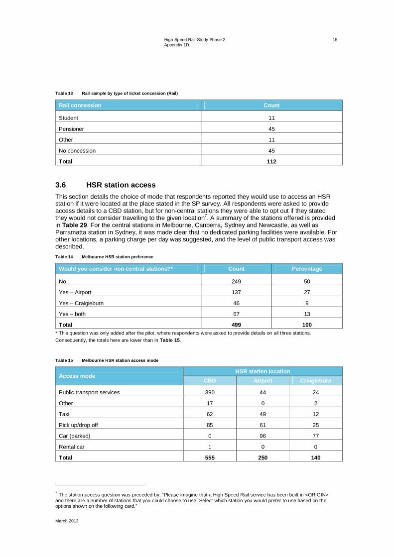
High Speed Rail Study Phase 2 Appendix 1D
March 2013
15
Table 13 Rail sample by type of ticket concession (Rail)
Rail concession Count
Student 11
Pensioner 45
Other 11
No concession 45
Total 112
3.6 HSR station access This section details the choice of mode that respondents reported they would use to access an HSR station if it were located at the place stated in the SP survey. All respondents were asked to provide access details to a CBD station, but for non-central stations they were able to opt out if they stated they would not consider travelling to the given location7. A summary of the stations offered is provided in Table 29. For the central stations in Melbourne, Canberra, Sydney and Newcastle, as well as Parramatta station in Sydney, it was made clear that no dedicated parking facilities were available. For other locations, a parking charge per day was suggested, and the level of public transport access was described. Table 14 Melbourne HSR station preference
Would you consider non-central stations?* Count Percentage
No 249 50
Yes – Airport 137 27
Yes – Craigieburn 46 9
Yes – both 67 13
Total 499 100 * This question was only added after the pilot, where respondents were asked to provide details on all three stations. Consequently, the totals here are lower than in Table 15.
Table 15 Melbourne HSR station access mode
Access mode HSR station location
CBD Airport Craigieburn
Public transport services 390 44 24
Other 17 0 2
Taxi 62 49 12
Pick up/drop off 85 61 25
Car (parked) 0 96 77
Rental car 1 0 0
Total 555 250 140
7 The station access question was preceded by: “Please imagine that a High Speed Rail service has been built in <ORIGIN> and there are a number of stations that you could choose to use. Select which station you would prefer to use based on the options shown on the following card.”

High Speed Rail Study Phase 2 Appendix 1D
March 2013
16
Table 16 Sydney HSR station preference
Would you consider non-central stations? Count Percentage
No 245 38
Yes – Parramatta 72 11
Yes – Homebush 246 38
Yes – Both 87 13
Total 650 100 Table 17 Sydney HSR station access mode
Access mode CBD Parramatta Homebush
Public transport services 479 114 102
Other 17 7 1
Taxi 92 9 22
Pick up/drop off 61 29 37
Car (parked) 0 0 160
Rental car 1 0 1
Total 650 130 323* * Ten people said they would use Homebush but then could not nominate an access mode.
Table 18 Canberra HSR station preference
Would you consider a non-central station? Count Percentage
No 54 22
Yes – Canberra Airport 197 78
Total 251 100 Table 19 Canberra HSR station access mode
Access mode Civic Airport
Public transport services 61 29
Other 12 0
Taxi 67 35
Pick up/drop off 110 71
Car (parked) 0 60
Rental car 1 0
Total 251 195* * Two people said they would use an airport station but then could not nominate an access mode.

High Speed Rail Study Phase 2 Appendix 1D
March 2013
17
Table 20 Albury-Wodonga HSR station preference
Would you consider a non-central station?* Count Percentage
No 32 21
Yes – 15 km north 118 79
Total 150 100 * This question was only added after the pilot, where respondents were asked to provide details on both stations. Consequently, the totals here are lower than in Table 21.
Table 21 Albury-Wodonga HSR station access mode
Access mode Central 15 km north
Public transport services 2 9
Other 20 9
Taxi 44 21
Pick up/drop off 62 43
Car (parked) 63 72
Rental car 0 0
Total 191 154 Table 22 Wagga Wagga HSR station preference
Would you consider a non-central station? Count Percentage
No 36 24
Yes – 20 km south 114 76
Total 150 100 Table 23 Wagga Wagga HSR station access mode
Access mode Central 20 km south
Public transport services 3 9
Other 11 3
Taxi 37 18
Pick up/drop off 51 38
Car (parked) 48 43
Rental car 0 0
Total 150 111 Table 24 Newcastle HSR station preference
Would you consider a non-central station? Count Percentage
No 38 13
Yes – 15 km west 262 87
Total 300 100

High Speed Rail Study Phase 2 Appendix 1D
March 2013
18
Table 25 Newcastle HSR station access mode
Access mode Central 15 km west
Public transport services 71 68
Other 52 2
Taxi 41 18
Pick up/drop off 135 66
Car (parked) 0 103
Rental car 1 0
Total 300 257* * Five people said they would use an outer station but then could not nominate an access mode.
3.7 HSR choices The following tables detail the choices respondents made with respect to HSR, such as the preferred class for business travellers (Table 26), the aspects of HSR that respondents most valued (Table 27), and how they would get from the HSR station at their destination city to their final destination (Table 28).
Table 26 Choice of HSR class, business travellers only
HSR class Count Percentage
Standard 361 80
Premium 88 20
Total 449 100 Table 27 Aspects of HSR most valued
Feature of HSR Ranking
1st 2nd 3rd
Speed 643 440 142
Comfort 322 406 235
Able to work 46 62 57
Direct to CBD 79 82 80
Wi-fi 15 54 98
Reliability 92 100 74
Safety 129 85 55
Avoids airport 77 80 65
Environment 68 55 38
Integrates with the wider public transport network 31 43 40
Other 596 312 142
Total 2098 1719 1026

High Speed Rail Study Phase 2 Appendix 1D
March 2013
19
The SP survey stated that the HSR station at the destination would be located in a central location. Respondents were asked how they would get from there to their final destination (Table 28).
Table 28 HSR egress mode (from a central station)
Destination
Egress mode
Walk Rental car
Pick up/ drop off Taxi
Bus/ local train
Other Total
Albury-Wodonga 18 9 44 42 13 2 128
Canberra 34 19 118 141 74 0 386
Sydney 113 25 58 200 495 13 904
Melbourne 50 14 31 88 189 3 375
Wagga Wagga 2 1 9 7 0 0 19
Newcastle 10 4 22 15 26 0 77
Port Macquarie 7 5 13 11 5 1 42
Gold Coast 4 16 10 20 14 1 65
Brisbane 11 12 21 15 33 3 95
Shepparton 2 0 4 0 1 0 7
Total 251 105 330 539 850 23 2098
The proportion of walk egress is usually 10 per cent or higher. For Sydney and Melbourne, local public transport egress is at least 50 per cent but for other destinations it is 20 per cent on average.
As found in the pilot survey, there continued to be strong support for HSR among respondents, as evidenced in the comments they made, particularly for those who chose HSR in every mode choice scenario.
4.0 Main survey – analysis of SP data Initially, the two SP experiments (station choice, mode choice) were analysed separately. Only ‘traders’8 were included, and the analysis was done separately for different markets. All models have been estimated using BIOGEME.
One of the features of SP analysis is that each respondent provides responses to a number of choice scenarios, so that the data has the quality of a panel, in that there may be significant variation in the choice behaviour between respondents leading to variations in their responses to the different travel contexts. In analysing the data, allowance should be made for possible ‘within respondent’ correlations in the random terms. Unfortunately, these can lead to long run times for estimation. Because of this, the general approach has been to check whether the key parameters are sensitive to a panel specification. If they are not, the analysis is conducted without allowing for the panel effect.
In section 4.1 the analysis of the station choice SP is briefly discussed. section 4.2 briefly discusses the mode choice analysis separately for the three current modes. Based on what has been learnt from this, section 4.3 then describes how the combined analysis was carried out.
8 Respondents who, faced with the nine choice tasks, chose differently on at least one occasion. Data for non-traders does not affect the statistical analysis.
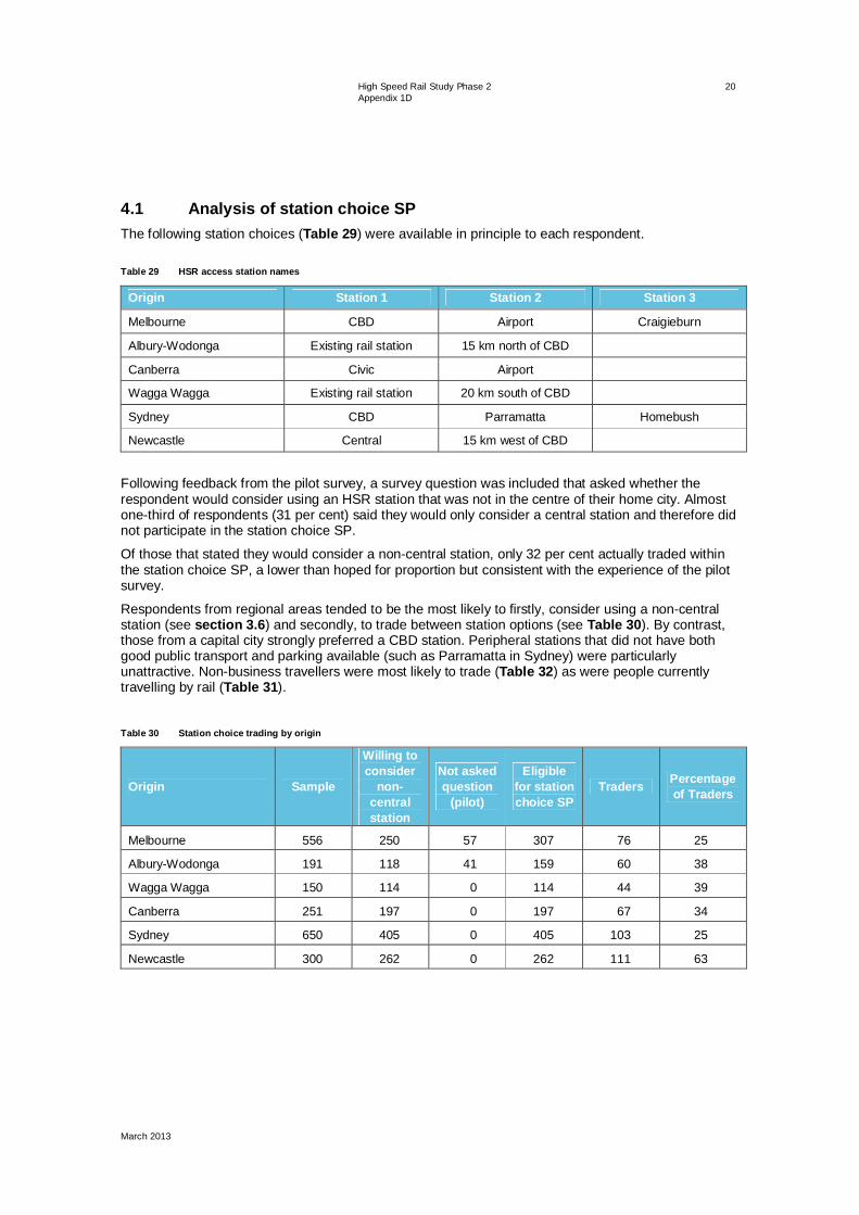
High Speed Rail Study Phase 2 Appendix 1D
March 2013
20
4.1 Analysis of station choice SP The following station choices (Table 29) were available in principle to each respondent. Table 29 HSR access station names
Origin Station 1 Station 2 Station 3
Melbourne CBD Airport Craigieburn
Albury-Wodonga Existing rail station 15 km north of CBD
Canberra Civic Airport
Wagga Wagga Existing rail station 20 km south of CBD
Sydney CBD Parramatta Homebush
Newcastle Central 15 km west of CBD
Following feedback from the pilot survey, a survey question was included that asked whether the respondent would consider using an HSR station that was not in the centre of their home city. Almost one-third of respondents (31 per cent) said they would only consider a central station and therefore did not participate in the station choice SP.
Of those that stated they would consider a non-central station, only 32 per cent actually traded within the station choice SP, a lower than hoped for proportion but consistent with the experience of the pilot survey.
Respondents from regional areas tended to be the most likely to firstly, consider using a non-central station (see section 3.6) and secondly, to trade between station options (see Table 30). By contrast, those from a capital city strongly preferred a CBD station. Peripheral stations that did not have both good public transport and parking available (such as Parramatta in Sydney) were particularly unattractive. Non-business travellers were most likely to trade (Table 32) as were people currently travelling by rail (Table 31).
Table 30 Station choice trading by origin
Origin Sample
Willing to consider
non-central station
Not asked question
(pilot)
Eligible for station choice SP
Traders Percentage of Traders
Melbourne 556 250 57 307 76 25
Albury-Wodonga 191 118 41 159 60 38
Wagga Wagga 150 114 0 114 44 39
Canberra 251 197 0 197 67 34
Sydney 650 405 0 405 103 25
Newcastle 300 262 0 262 111 63
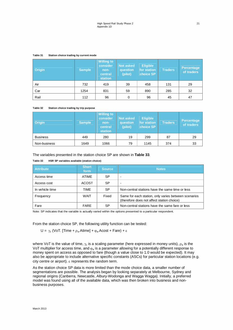
High Speed Rail Study Phase 2 Appendix 1D
March 2013
21
Table 31 Station choice trading by current mode
Origin Sample
Willing to consider
non-central station
Not asked question
(pilot)
Eligible for station choice SP
Traders Percentage of traders
Air 732 419 39 458 131 29
Car 1254 831 59 890 285 32
Rail 112 96 0 96 45 47 Table 32 Station choice trading by trip purpose
Origin Sample
Willing to consider
non-central station
Not asked question
(pilot)
Eligible for station choice SP
Traders Percentage of traders
Business 449 280 19 299 87 29
Non-business 1649 1066 79 1145 374 33
The variables presented in the station choice SP are shown in Table 33.
Table 33 HSR SP variables available (station choice)
Attribute Short form Source Notes
Access time ATIME SP -
Access cost ACOST SP -
In vehicle time TIME SP Non-central stations have the same time or less
Frequency WAIT Fixed Same for each station, only varies between scenarios (therefore does not affect station choice)
Fare FARE SP Non-central stations have the same fare or less Note: SP indicates that the variable is actually varied within the options presented to a particular respondent.
From the station choice SP, the following utility function can be tested:
U = c (VoT. [Time + a.Atime] + a.Acost + Fare) +
where VoT is the value of time, c is a scaling parameter (here expressed in money units), a is the VoT multiplier for access time, and a is a parameter allowing for a potentially different response to money spent on access as opposed to fare (though a value close to 1.0 would be expected). It may also be appropriate to include alternative specific constants (ASCs) for particular station locations (e.g. city centre or airport). represents the random term.
As the station choice SP data is more limited than the mode choice data, a smaller number of segmentations are possible. The analysis began by looking separately at Melbourne, Sydney and regional origins (Canberra, Newcastle, Albury-Wodonga and Wagga Wagga). Initially, a preferred model was found using all of the available data, which was then broken into business and non-business purposes.

High Speed Rail Study Phase 2 Appendix 1D
March 2013
22
Three models were tested with all purposes combined:
Basic (x1).
Panel ASC (x4).
Panel ASC allowing for ASC correlation (x5) (not for regional station choice).
The Panel ASC model allows for an additional individual-specific random term to be attached to each station ASC, with variance to be estimated, as a way of allowing for ‘repeated observations’. In model x4 these terms are assumed to be independent, but in model x5, for Sydney and Melbourne where there are multiple options, they are allowed to be correlated, and the extent of correlation is treated as an additional parameter to be estimated. Essentially the ASC parameters are estimated as multi-variate normally distributed: for model x4 the variance matrix has only diagonal entries, but for model x5 off-diagonal elements relating separately to the Sydney and Melbourne ASCs are added. In the tables, the terms sasc represent the square root of the ASC variances, while the ‘ASC correlations’ are calculated as the ratio of the off-diagonal element to the product of the standard deviations on the diagonal.
Given that the models for Sydney and regional origins both looked sensible, as did Melbourne after some adjustment, a combined model was estimated as shown in Table 34, in which separate ASCs are estimated for the various non-central stations, but other parameters are the same regardless of origin. Since for both Sydney and Melbourne the x5 model was preferred to x4, x4 was not estimated for the combined model and x5 was chosen to represent the ‘panel effect’. Different scaling has also been allowed for, relative to Sydney: for the regional origins the scale is not significantly different from 1, but for Melbourne it is significantly lower, indicating a greater randomness. This means that the variations between individuals in the sample in the way stations are selected are greater for Melbourne than elsewhere.
In reporting the estimation results, square brackets contain the parameter symbols which were used in the utility equation, but for ease of understanding a somewhat expanded description of the parameter is also given in the first column. Commentary on the results follows the table.
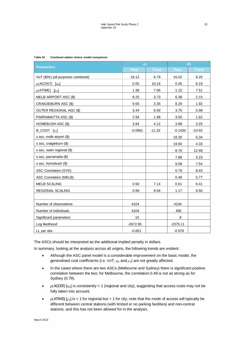
High Speed Rail Study Phase 2 Appendix 1D
March 2013
23
Table 34 Combined station choice, model comparison
Parameters x1 X5
Para T-test Para T-test
VoT ($/hr) (all purposes combined) 18.12 6.79 16.02 8.25
ACOST) [ a] 0.55 10.16 0.45 8.19
ATIME) [ a] 1.38 7.06 1.15 7.51
MELB AIRPORT ASC ($) 8.25 3.73 6.38 2.15
CRAIGIEBURN ASC ($) 9.55 3.35 8.29 1.92
OUTER REGIONAL ASC ($) 3.44 6.59 3.75 5.98
PARRAMATTA ASC ($) 2.94 1.98 3.50 1.62
HOMEBUSH ASC ($) 3.84 4.12 3.88 3.25
B_COST [ C] -0.0961 -11.32 -0.1420 -10.93
sasc, melb airport ($) 18.30 6.34
sasc, craigieburn ($) 19.60 4.33
sasc, outer regional ($) 8.76 12.68
sasc, parramatta ($) 7.88 3.23
sasc, homebush ($) 9.08 7.54
ASC Correlation (SYD) 0.79 8.43
ASC Correlation (MELB) 0.48 5.77
MELB SCALING 0.50 7.14 0.61 6.41
REGIONAL SCALING 0.99 9.94 1.17 9.50
Number of observations 4104 4104
Number of individuals 4104 456
Significant parameters 10 8
Log likelihood -2672.95 -2375.11
LL per obs -0.651 -0.579
The ASCs should be interpreted as the additional implied penalty in dollars.
In summary, looking at the analysis across all origins, the following trends are evident:
Although the ASC panel model is a considerable improvement on the basic model, the generalised cost coefficients (i.e. VoT, a and a) are not greatly affected.
In the cases where there are two ASCs (Melbourne and Sydney) there is significant positive correlation between the two; for Melbourne, the correlation 0.48 is not as strong as for Sydney (0.79).
ACOST) [ a] is consistently < 1 (regional and city), suggesting that access costs may not be fully taken into account.
ATIME) [ a] is < 1 for regional but > 1 for city; note that the mode of access will typically be different between central stations (with limited or no parking facilities) and non-central stations, and this has not been allowed for in the analysis.

High Speed Rail Study Phase 2 Appendix 1D
March 2013
24
The mean ASCs are small (all < $10), though the significant positive values imply a disadvantage relative to the central station. However, as noted, there is considerable individual-specific ASC variation, suggesting that the population is divided between those favouring a central station and those favouring a non-central station.
Values of time generally look reasonable (though without constraining the access time Melbourne VoTs were low); when segmenting by purpose, business had higher values
than leisure.
4.2 Analysis of mode choice SP data (all modes) The mode choice presented to each respondent was a binary choice between their current mode and HSR.
The total proportion of trading between HSR and the current mode was 65 per cent of the sample, with three quarters of the non-traders choosing HSR in every scenario. The following tables provide a breakdown of who the non-traders9 are.
Respondents currently travelling by air were more likely to trade than those travelling by car, while rail passengers (Newcastle-Sydney) overwhelmingly switched to HSR (Table 35). Car travellers were the most likely to choose only their current mode, predominantly due to the convenience of having a car at the destination end of their journey. The study did not collect car ownership data, but according to Table 10, 152 of the air travellers and 35 of the rail travellers did consider the car mode. Table 35 Non-traders by mode
Mode Total sample Non-traders Among non-traders, HSR only
Count Percentage Count Percentage
Air 732 224 31 203 91
Car 1254 438 35 278 63
Rail 112 69 62 66 96
Total 2098 731 35 547 75
People in regional areas (Albury-Wodonga and Canberra) typically traded more than those based in Melbourne or Sydney (Table 36). Note that the Newcastle sample contains a large portion of rail journeys (112 out of 300) which were less inclined to trade. The high proportion of non-traders in Wagga Wagga is due to an issue discovered early in the survey, which resulted in the HSR service presented being too attractive. This was subsequently modified, resulting in much more trading. Table 36 Non-traders by origin
Origin Total sample Non-traders Among non-traders, HSR only
Count Percentage Count Percentage
Melbourne 556 196 35 148 76
Albury-Wodonga 191 42 22 21 50
Wagga Wagga 150 66 44 60 91
Canberra 251 54 22 35 65
Sydney 650 227 35 151 67
Newcastle 300 146 49 132 90
9 In addition to non-traders, 23 observations noted as having extreme or incorrect values have been removed for the mode choice estimation (18 currently travelled by car, and five by air).

High Speed Rail Study Phase 2 Appendix 1D
March 2013
25
Respondents travelling to large centres such as Melbourne, Brisbane and the Gold Coast were more likely to trade than those travelling to regional areas (Table 37). Table 37 Non-traders by destination
Destination Total sample Non-traders Among non-traders, HSR only
Count Percentage Count Percentage
Albury-Wodonga 128 48 38 21 44
Canberra 386 130 34 86 66
Sydney 904 327 36 275 84
Melbourne 375 114 30 93 82
Wagga Wagga 19 10 53 8 80
Newcastle 77 41 53 23 56
Port Macquarie 42 17 40 7 41
Gold Coast 65 17 26 13 76
Brisbane 95 24 25 20 83
Shepparton 7 3 43 1 33
As found in the pilot survey, it was difficult to make people travelling over short distances trade (Table 38), though the non-traders were mainly only choosing HSR rather than their current mode (mainly car). In addition, the short regional sample includes respondents from both Wagga Wagga-Canberra and Newcastle-Sydney rail trips, which both had high incidences of choosing HSR only. Respondents making long regional trips (typically over 250 kilometres and not between capital cities) were the most likely to trade. Of those that did not trade, there was a much higher incidence of people remaining with their current mode for long regional trips, compared with the other two markets.
Table 38 Non-traders by distance
Distance Total sample
Non-traders Among non-traders, HSR only Count Percentage Count Percentage
Intercity 854 285 33 247 87
Short regional 411 225 55 190 84
Long regional 833 221 27 110 50
Business travellers (about 21 per cent of the sample) were slightly more likely not to trade (Table 39). Table 39 Non-traders by purpose
Purpose Sample Non-traders Among non-traders, HSR only
Count Percentage Count Percentage
Business 449 181 40 133 73
Non-business 1649 550 33 414 75
Looking at the data by mode, distance and purpose at the same time (Table 40) shows that the air-long regional sample is the most likely to trade, while, among the non-traders, air inter-capital and rail short regional were likely to choose HSR in every scenario. For car, short regional journey trading occurred less than half of the time. There is only a small difference between purposes, with business slightly more likely not to trade.

High Speed Rail Study Phase 2 Appendix 1D
March 2013
26
Table 40 Non-traders by mode, distance and purpose
Mode Distance Purpose Sample Non-traders Among non-traders,
HSR only Count Percentage Count Percentage
Air Inter-capital Business 260 104 40 95 91
Air Inter-capital Non-business 360 104 29 96 92
Air Long regional Business 49 7 14 6 86
Air Long regional Non-business 63 9 14 6 67
Car Inter-capital Business 5 2 40 0 0 Car Inter-capital Non-business 229 75 33 56 75 Car Long regional Business 71 30 42 6 20 Car Long regional Non-business 650 175 27 92 53 Car Short regional Business 48 27 56 16 59 Car Short regional Non-business 251 129 51 108 84
Rail Short regional Business 16 11 69 10 91
Rail Short regional Non-business 96 58 60 56 97
The variables presented in the mode choice SP are shown in Table 41. Table 41 SP variables available (mode choice)
Attribute Short form HSR Air Standard rail Car
Access time ATIME SP RP RP N/A
Access cost ACOST SP RP RP N/A
Check-in time CHECK Constant SP None N/A
In vehicle time TIME SP SP SP SP
Frequency WAIT SP SP SP N/A
Fare FARE/COST SP SP SP SP
Class CLASS Fixed RP RP N/A
Egress time ETIME RP RP RP N/A
Egress cost ECOST RP RP RP N/A Note: SP indicates that the variable is actually varied within the options presented, while RP indicates that the variables are fixed for all the options presented, but can still vary between individuals (RP data). This reflects the fact that the options presented in the SP were in the context of a particular sampled journey: with the exception of HSR station choice, it was not considered realistic to modify the access and egress arrangements.
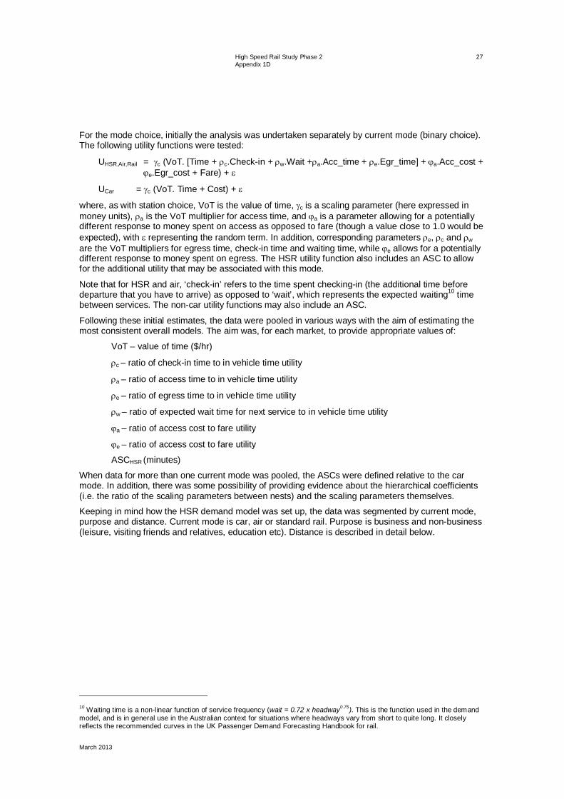
High Speed Rail Study Phase 2 Appendix 1D
March 2013
27
For the mode choice, initially the analysis was undertaken separately by current mode (binary choice). The following utility functions were tested:
UHSR,Air,Rail = c (VoT. [Time + c.Check-in + w.Wait + a.Acc_time + e.Egr_time] + a.Acc_cost + e.Egr_cost + Fare) +
UCar = c (VoT. Time + Cost) +
where, as with station choice, VoT is the value of time, c is a scaling parameter (here expressed in money units), a is the VoT multiplier for access time, and a is a parameter allowing for a potentially different response to money spent on access as opposed to fare (though a value close to 1.0 would be expected), with representing the random term. In addition, corresponding parameters e, c and w are the VoT multipliers for egress time, check-in time and waiting time, while e allows for a potentially different response to money spent on egress. The HSR utility function also includes an ASC to allow for the additional utility that may be associated with this mode.
Note that for HSR and air, ‘check-in’ refers to the time spent checking-in (the additional time before departure that you have to arrive) as opposed to ‘wait’, which represents the expected waiting10 time between services. The non-car utility functions may also include an ASC.
Following these initial estimates, the data were pooled in various ways with the aim of estimating the most consistent overall models. The aim was, for each market, to provide appropriate values of:
VoT – value of time ($/hr)
c – ratio of check-in time to in vehicle time utility
a – ratio of access time to in vehicle time utility
e – ratio of egress time to in vehicle time utility
w – ratio of expected wait time for next service to in vehicle time utility
a – ratio of access cost to fare utility
e – ratio of access cost to fare utility
ASCHSR (minutes)
When data for more than one current mode was pooled, the ASCs were defined relative to the car mode. In addition, there was some possibility of providing evidence about the hierarchical coefficients (i.e. the ratio of the scaling parameters between nests) and the scaling parameters themselves.
Keeping in mind how the HSR demand model was set up, the data was segmented by current mode, purpose and distance. Current mode is car, air or standard rail. Purpose is business and non-business (leisure, visiting friends and relatives, education etc). Distance is described in detail below.
10 Waiting time is a non-linear function of service frequency (wait = 0.72 x headway0.75). This is the function used in the demand model, and is in general use in the Australian context for situations where headways vary from short to quite long. It closely reflects the recommended curves in the UK Passenger Demand Forecasting Handbook for rail.

High Speed Rail Study Phase 2 Appendix 1D
March 2013
28
Table 42 shows the highway distances (city centre to city centre) between all of the OD pairs included in the survey. The highlighting shows how the OD pairs have been classified into three distance/city type categories consistent with the HSR demand model. Table 42 Distance matrix (kilometres between origin and destination for surveyed movements)
Destination Origin
Melbourne Albury-Wodonga
Wagga Wagga Canberra Sydney Newcastle
Melbourne 327 666 878 Shepparton 189 Albury-Wodonga 327 350 554 Wagga Wagga 245 458 Canberra 666 350 245 290 438 Sydney 878 554 458 290 158 Newcastle 438 158 Port Macquarie 384 Gold Coast 840 Brisbane 938 789
Short regional (< 250 km)
Long regional
Inter-capital(> 600 km)
Data was analysed by mode (all purposes and distances combined) and then by individual segments. As noted, when analysing by mode (on a binary basis), the ASC is attached to the HSR option.
Three types of models were tested, with some variations around these by fixing non-significant rho ( ‘ratio’ parameters to 1.0:
Basic (x1).
Panel ASC (x4).
Distributed VOT (x6).
The x4 model allows for an additional individual-specific random term to be attached to the ASC, with variance to be estimated (‘repeated observations’). For the mode choice analysis, another form of panel model (x6) was considered in which the Value of Time follows a lognormal distribution. This requires two parameters to be estimated from which the mean and the coefficient of variation (CV, ratio of the standard deviation to the mean) of the distribution can be calculated. The variance parameter actually reported is referred to as svot11.
For each mode, the preferred model was chosen and then run separately for the distance/purpose segments. However, the rail sample consisted primarily of non-business travellers (38 out of 43 once non-traders were removed) and therefore only represents the short regional, non-business, rail travel market. These models are presented in the tables below. As with the station choice models, in reporting the estimation results, square brackets contain the parameter symbols which were used in the utility equation, but for ease of understanding a somewhat expanded description of the parameter is also given in the first column. Commentary on the results follows the tables.
11 CV may be calculated by means of the formula CV = (exp ( 2)–1), where = svot.

High Speed Rail Study Phase 2 Appendix 1D
March 2013
29
Table 43 Air, preferred model (x4) segmented by distance and purpose
Parameters
Intercapital – business
Long regional –business
Inter-capital – non-business
Long regional – non-business*
Para-meter T-test Para-
meter T-test Para-meter T-test Para-
meter T-test
VoT ($/hr) 78.00 12.19 60.00 5.15 18.90 7.94 32.16 2.70
ACOST) [ a] 0.5 3.21 0.5 1.22 0.2 2.65 0.2 0.50
ATIME) [ a] 0.4 1.89 0.7 1.22 0.9 2.88 -0.1 -0.05
ECOST) [ e] 0.5 1.76 0.7 1.36 0.3 2.57 0.5 0.85
ETIME) [ e] 1.0 fixed 1.0 fixed 1.0 fixed 0.9 0.97
WAIT) [ w] 0.3 1.14 0.5 1.32 1.3 2.52 0.5 0.93
CHECK) [ c] 0.6 3.01 0.9 2.35 0.7 2.87 0.4 0.86
HSR ASC ($) 2.15 5.04 1.99 2.21 1.89 5.92 -57.30 -3.71
B_COST [ C] -0.03 -13.66 -0.04 -7.28 -0.05 -19.06 -0.04 -8.70
sasc ($) 1.61 9.50 2.26 5.14 1.65 12.04 50.50 5.46
svot
Number of obs. 1386 369 2286 486
Number of ind. 154 41 254 54
Signif. params. 6 5 9 4
Log likelihood -595.2 -148.1 -977.4 -208.5
LL per obs -0.429 -0.401 -0.428 -0.429 * Did not converge, so results are only indicative of parameter values. Note: Air is not relevant for short regional movements.

High Speed Rail Study Phase 2 Appendix 1D
March 2013
30
Table 44 Rail, all purposes and distances, preferred mode choice model
Parameters x6_fixed
Parameter T-test
VoT ($/hr) - mean 19.49 4.58
ACOST) [ a] 1.0 fixed
ATIME) [ a] 1.1 2.60
ECOST) [ e] 1.0 fixed
ETIME) [ e] 1.0 fixed
WAIT) [ w] 1.0 fixed
CHECK) [ c]
HSR ASC ($) 2.29 0.73
B_COST [ C] -0.138 -4.58
sasc ($)
svot 0.672 4.73
Number of observations 387
Number of individuals 43
Significant parameters 4
Log likelihood -197.21
LL per obs -0.510
In none of the estimated models for rail was the HSR ASC significantly different from zero (Table 44 above). As noted above, this model is considered to apply to the short regional, non-business, rail travel market.

High Speed Rail Study Phase 2 Appendix 1D
March 2013
31
Table 45 Car, preferred model (x6) for non-business segmented by distance
Parameters
Short regional – non-business
Long regional – non-business
Inter-capital – non-business*
Para-meter T-test Para-
meter T-test Para-meter T-test
VoT ($/hr) 16.97 7.42 22.53 17.30 14.23 8.87
ACOST) [ a] 1.0 fixed 1.0 fixed 1.0 fixed
ATIME) [ a] 0.9 3.44 0.8 5.74 -1.3 -2.02
ECOST) [ e] 1.0 fixed 1.0 fixed 1.0 fixed
ETIME) [ e] 0.4 1.78 -0.7 -2.90 0.6 1.15
WAIT) [ w] 0.0 fixed 0.0 fixed 0.0 fixed
CHECK) [ c] 1.0 fixed 1.0 fixed 1.0 fixed
HSR ASC ($) 8.09 2.14 -1.80 -0.84 -0.90 -0.11
B_COST [ C] -0.09 -11.07 -0.05 -24.02 -0.03 -12.48
sasc ($)
svot 0.50 4.82 1.03 15.90 0.74 9.13
Number of obs. 1098 4221 1296
Number of ind. 122 469 144
Signif. params. 5 5 4
Log likelihood -573 -2072 -634
LL per obs# -0.522 -0.491 -0.490 * Did not converge, so results are only indicative of parameter values # LL is abbreviation for Log Likelihood

High Speed Rail Study Phase 2 Appendix 1D
March 2013
32
Table 46 Car, preferred model (x6) for business segmented by distance
Parameters Short regional –
business* Long regional –
business* Parameter T-test Parameter T-test
VoT ($/hr) 45.76 2.57 264.91 1.35
ACOST) [ a] 1.0 fixed 1.0 fixed
ATIME) [ a] -0.1 -0.08 1.4 1.94
ECOST) [ e] 1.0 fixed 1.0 fixed
ETIME) [ e] 1.0 2.20 1.7 7.86
WAIT) [ w] 0.0 fixed 0.0 fixed
CHECK) [ c] 1.0 fixed 1.0 fixed
HSR ASC ($) -0.41 -0.02 1.18 0.02
B_COST [ C] -0.03 -4.46 0.00 -3.17
sasc ($)
svot 0.70 3.13 1.39 1.88
Number of obs. 189 369
Number of ind. 21 41
Signif. params. 3 2
Log likelihood -107 -228
LL per obs# -0.569 -0.618 *Did not converge, so results are only indicative of parameter values. # LL is abbreviation for Log Likelihood
It can be seen that while the key values of time are generally sensible, less plausible values (and in some cases, wrongly signed) for the other generalised cost weights (access, egress, etc.) were obtained in a number of cases, leading to some constraints being imposed. This is a general issue that is addressed in Section 5.3. It should be borne in mind that, as set out in Table 41, some of these variables only had limited variation.
4.3 Combined estimation Having obtained generally plausible results from the individual choice tasks, the next stage was to pool all the data, and this led to questions as to how the mode choice and station choice tasks should be structured. In the demand model, the station choice model was conditional on the choice of HSR, and this suggested a nested structure. However, it was decided to adopt a non-nested structure as shown in Figure 8. This reflects that, while the two SPs are linked, the respondent is never directly presented with the choice between multiple HSR stations and their current mode. Instead, there are two distinct steps: (a) choose an HSR station (b) compare this HSR choice to the current mode. A scale factor has therefore been estimated for the station choice experiment (with the expectation that this will be > 1), which results in seven options, the three station choices, and four higher mode choices. This avoids the loss of information from the station choice data when HSR is not selected in the mode choice when estimating a fully nested model.

High Speed Rail Study Phase 2 Appendix 1D
March 2013
33
Figure 8 Non-nested structure for combined mode and station choice estimation
A number of variants were examined. The general assumption in transport forecasting models is that scaling parameters will be held constant in time units, with allowances for increases in VoT reflecting rising income. For convenience, most of the detailed (segmented) analysis has kept the scaling parameters in money units, but the combined analysis models were estimated in both time and money units. The models based on time units were marginally preferred, and since this corresponds with the forecasting requirements, these have been retained.
The general specification for this model has the form:
sec,sec,,1 /.. purppurpTSP VoTCT The T and C terms denote all the relevant cost and time elements, including ASCs.
This specification allows both scaling parameter T and value of time V to vary with purpose and distance sector. The parameter SP1 allows for a different scale to apply to the station choice data.
As written, the notation implies that a separate scaling parameter and value of time were estimated for each combination of purpose and sector. In fact, a slightly more parsimonious approach to estimation was adopted, treating the two effects as independent and multiplicative. In both cases, the estimated basic parameters ( T and value of time V) relate to the non-business purpose and the inter-capital distance. The ‘ ’ parameters modify these parameters for the business purpose, and the ‘p’ parameters modify them for the other distances.
Thus, for the scaling parameter ,sec, purpT was estimated as:
SLTBusTT p
,secsecsec, .1..
and the Value of time sec,purpVoT was estimated
as:
SLBus pVV
,secsecsec .1..
where ‘Bus’ indicates Business purpose and ‘sec’ relates to distance, and the (0,1) variables indicate whether the category applies.
STN1
RAIL
STN3
HSR
STN2
CAR AIR

High Speed Rail Study Phase 2 Appendix 1D
March 2013
34
As a result, the overall specification can be expanded to:
SLBus
SLTBusTTSP
pVV
CTp
,secsecsec
,secsecsec,1
.1....1...
The overall model (y10a) seems generally to replicate the previous separate analysis, and the ‘expt 1’ parameter is much greater than 1, showing that the station choice SP is more deterministic than the mode choice SP. The ASC analysis is very similar to what was obtained both on the station choice and on the mode choice and the counter-intuitive results for the rho ( ) values have largely disappeared, though the access and egress multipliers may still be considered on the low side.
The results (Table 47) show that, although the long regional value of time remains significantly higher than inter-capital, the scaling parameters are now in line with expectations and this is the final combined model tested.
In this table, parameters prefixed with ‘d’ are intended to be added to the basic parameter according to particular segments (thus, for example, the parameter dVOTbus is added to the basic parameter VOT when the respondent is a business traveller). Correspondingly, parameters prefixed with ‘ ’ should have 1 added to them as a weight before combining with the generic time or cost variables. ASCs apply to all modes except car12. Note that, in this model, the ASCs for air and HSR have not been segmented by distance, only by purpose. An additional column of commentary is provided on these results.
12 These parameters are estimated as the additional weighting relative to IVT. For example, if walking time is 2.5*IVT, p would be 1.5 etc. This allows significant difference from IVT (p = 0) to be easily assessed.
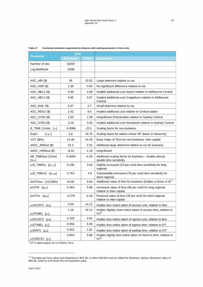
High Speed Rail Study Phase 2 Appendix 1D
March 2013
35
Table 47 Combined estimation segmented by distance with scaling parameter in time units
Parameter y10a
Parameter T-test Comments
Number of obs. 16200
Log-likelihood -9186
ASC_AIR ($) 36 10.02 Large deterrent relative to car
ASC_HSR ($) 1.36 0.83 No significant difference relative to car
ASC_MEL2 ($) 5.99 4.08 Implied additional cost Airport relative to Melbourne Central
ASC_MEL3 ($) 6.85 3.57 Implied additional cost Craigieburn relative to Melbourne Central
ASC_RAIL ($) 5.97 2.7 Small deterrent relative to car
ASC_REG2 ($) 2.42 6.5 Implied additional cost relative to Central station
ASC_SYD2 ($) 1.93 1.38 Insignificant (Parramatta) relative to Sydney Central
ASC_SYD3 ($) 3.18 3.45 Implied additional cost Homebush relative to Sydney Central
B_TIME (1/min) [ T] -0.0066 -22.5 Scaling factor for non-business
Expt1 [ SP1] 2.8 16.75 Scaling factor for station choice SP (lower in hierarchy)
VOT ($/hr) 14.46 24.45 Base Value of Time for non-business, inter-capital
dASC_AIRbus ($) 32.2 2.91 Additional large deterrent relative to car for business
dASC_HSRbus ($) -8.03 -1.19 Insignificant
dB_TIMEbus (1/min) [ T]
-0.0056 -6.34 Additional scaling factor for business – implies almost double time sensitivity
B_TIMElr) [pT,LR] 0.236 3.26 Slightly increased (23 per cent) time sensitivity for long regional
B_TIMEsr) [pT,SR] 0.763 4.9 Substantially increased (76 per cent) time sensitivity for short regional
dVOTbus [ V] ($/hr) 43.80 9.83 Additional value of time for business (implies a factor of 4)13
pVOTlr [pLR] 0.464 5.88 Increased value of time (46 per cent) for long regional relative to inter-capital
pVOTsr [pSR] -0.275 -4.16 Reduced value of time (28 per cent) for short regional relative to inter-capital
ACOST) [ a] 0.59 14.12 Implies less notice taken of access cost, relative to fare
ATIME) [ a] 1.16 15.14 Implies slightly more notice taken of access time, relative to
IVT#
ECOST) [ e] 0.328 4.62 Implies less notice taken of egress cost, relative to fare
ETIME) [ e] 0.659 6.09 Implies less notice taken of egress time, relative to IVT
WAIT) [ w] 0.402 1.81 Implies less notice taken of waiting time, relative to IVT
CHECK) [ c] 0.843 5.88 Implies slightly less notice taken of check-in time, relative to
IVT#
# IVT is abbreviation for In-Vehicle Time
13 The base per hour value (non-business) is $14.46, to which $43.80 must be added for Business, giving a Business value of $58.26, which is 4.03 times the non-business value.

High Speed Rail Study Phase 2 Appendix 1D
March 2013
36
The SP can also be used to confirm that the mode choice hierarchy used in the demand model (see Figure 9) is the best hierarchy to adopt. For the purpose of this investigation the station choice data was omitted. The following four combinations have been tested in the lower nest:
a) Air and HSR.
b) Car and HSR.
c) Rail and HSR.
d) Air, rail and HSR.
However, it should be noted that, since all availability sets are binary, the scope for testing the hierarchy is very limited. Essentially, the scaling parameters for car, rail and air are being compared. The results provide some comfort that the scaling is higher (more deterministic) for air, and this is in line with the assumed RP model. They suggest that a nesting parameter of 1.3-1.4 is appropriate with the lower nest parameter being more sensitive for the inter-capital journeys. The short regional model does not need to be nested (as air is not available). Figure 9 Nested structure for combined mode choice estimation (as in demand model)
5.0 Recommendation on coefficients and implementation for demand model
As can be seen from the above commentary, the overall analysis of the SP is complex, because of a) the two experiments, b) the potential differing response by current mode, and c) different segments, particularly in relation to journey length. As set out in earlier sections, the approach has been first to carry out separate analyses, and then to try and estimate overall models.
A particular issue is the relationship between the scaling factors and the values of time, and how they vary with journey length. This issue (sometimes referred to as ‘cost damping’) is currently a topic of discussion in modelling. It is obvious from the analysis that has been carried out that there is considerable correlation between the scaling factor and the VoT, and also that different results can be obtained according to whether the scaling factor is cast in time or money units. Of course, this only becomes an issue when one starts trying to segment the effects.
The primary focus is on values of time and on the ASC for HSR, since it is considered that this is where the SP has the largest contribution to make. The conclusions are based on a mixture of statistical indicators and a priori expectations. On grounds of practicality, no attempt has been made to build a single model allowing for all possible effects. However, when there is some uncertainty about the stability of the results, this is indicated.
RAIL CAR
HSR AIR

High Speed Rail Study Phase 2 Appendix 1D
March 2013
37
The general list of issues where the SP can make some contribution to the overall demand model is as follows:
a) Scaling parameters.
b) Choice hierarchy.
c) Generalised cost specification, including access/egress.
d) Value of Time.
e) HSR ASCs.
f) Station choice issues (ASCs).
g) The variation in all of these by i) purpose and ii) distance.
The approach taken is that the overall demand model specification will be retained, and the SP results used to enhance it where appropriate.
5.1 Scaling parameters Based on the coefficients estimated for the combined estimation model (see Table 47) the following values were obtained:
Scaling factors (time units)
Non-business inter-capital: -0.00662
Non-business Long Regional: -0.00662 * 1.236 = –0.0082
Non-business Short Regional: -0.00662 * 1.763 = –0.0117
Business inter-capital: -0.00662 – 0.00561 = –0.01223
Business Long Regional: -0.01223 * 1.236 = –0.0151
Business Short Regional: -0.01223 * 1.763 = –0.0216
Although values of time and ASCs are also available from this model, it is considered more appropriate for them to be separately estimated for each distance/purpose combination, using the scaling parameters obtained in the combined SP analysis. This is discussed below.
In relation to the scaling factors, it is noteworthy that when expressed in time units, the Business values are larger, suggesting a greater sensitivity to time, or a lower variance (in time units) indicating fewer random (non-modelled) effects on choice.
With regard to the distance effect, the SP data supports an increase in the sensitivity with declining distance. The ratio of LR to inter-capital is 1.236 from the SP data and the ratio of SR to inter-capital is 1.763. This general relationship with distance is consistent with the international evidence (see box overleaf). It is generally considered that the scaling factors obtained from an SP analysis should not be directly used for a demand model, but should be re-scaled using data relating to actual choices (RP). There are two sources of data available for this – the somewhat limited RP data collected in the SP survey, and the more extensive data from the NVS. Both data sources have been used, but greater confidence is placed in the NVS analysis. The RP analysis should also be used to determine the appropriate ASCs for existing modes.
The approach taken was firstly to reach conclusions about the appropriate generalised cost specification from the SP analysis and then, using the relative scaling parameters given above, to estimate an overall scale to make the demand responsiveness to generalised cost compatible with the RP data. The results of this re-scaling are given in Section 5.5.

High Speed Rail Study Phase 2 Appendix 1D
March 2013
38
International evidence of the variation of scaling parameters with distance The expected values of the scaling parameters of the logit model were reviewed in the HSR context. With generalised times expressed in units of minutes, scaling parameters are directly comparable (and, where appropriate, transferable) between studies/models.
The scaling parameter values in the table below confirm the expected trend of reducing parameter values as distances increase: from 0.04 to 0.08 for metropolitan journeys to around 0.02 for long-distance inter-city journeys. Despite this variation, there is a large degree of consistency in the broad magnitude of the scaling parameters.
International evidence on the values of the scaling parameters used in inter-city/interurban travel demand studies
Source Mode choices Values of scaling parameters (trip purpose)
Inter-city/long-distance
EC (SDG, 2006) Air/HSR 0.010
US/Texas (Brand et al) Air/car 0.009, 0.022 (business); 0.005, 0.029 (non-business)
PBKA (MVA, 1986) Air/rail/car
0.007, 0.008, 0.011 (business)
HST-OOST (international), the Netherlands 0.02 (business); 0.01, 0.02 (other)
Regional medium distance
Speedrail Study: Sydney-Canberra trips Air/HSR/other 0.02 (business), 0.013 (other)
Regional short distance
Speedrail Study: intermediate trips HSR/other 0.037 (business), 0.017 (other)
Regional Fast Rail Study, Victoria Car/rail
0.014 (other)
LDTM, The Netherlands (MVA, 1985) 0.05, 0.04 (Business); 0.017, 0.03 (optional)
Metropolitan models
Melbourne Integrated Travel Model (MITM) Car/PT
0.05, 0.08 (other)
Auckland Regional Transport Model (ART3) 0.04 (other)
Notes: Costs in units of minutes. Where more than one scaling parameter value is given, the scaling parameter (the factor applied to generalised time) varies by mode, and the range of values used is indicated in the table (in no particular order).
References
EC report by SDG: Air and Rail Competition and Complementarity, 2006.
Daniel Brand et al., Forecasting High-Speed Rail Ridership, Transportation Research Record 1341, 1992.
Paris-Brussels-Cologne/Amsterdam Study, Forecasts of Air Travel, The MVA Consultancy 1986.
The Long Distance Travel Model for the Netherlands, Coefficients and other Parameters used in the Model, The MVA Consultancy, 1985.

High Speed Rail Study Phase 2 Appendix 1D
March 2013
39
5.2 Modal hierarchy Regarding the modal hierarchy, the SP data can only provide weak information, but the analysis in Section 4.3 suggested that the choice between HSR and air had a higher scaling parameter (by a factor of about 1.4).
The SP analysis also suggests a global scaling factor of 2.8 for the station choice process relative to the mode choice. This strongly supports the fact that station choice is more sensitive to time than mode choice.
5.3 Generalised cost weights Turning now to the generalised cost components, the combined SP analysis [y10a] (see Table 48) delivers the following weights (the existing assumptions from the demand model are presented for comparison): Table 48 Generalised cost coefficients (same for all modes, purposes and distances)
Coefficient Demand model SP t-ratio of difference from 1.0
Access time [ a] 2.0 1.16 2.09
Access cost [ a] 1.0 0.59 9.81
Check-in time[ c] 1.0 0.843 1.10
Wait time* [ w] 2.0 0.402 2.69
In-vehicle time 1.0 1
Fare 1.0 1
Egress time [ e] 2.0 0.659 3.15
Egress cost [ e] 1.0 0.328 9.47
* Applied to non-linear transformation of headway.
With the exception of check-in time, the SP values are all significantly on the low side, and therefore merit some discussion. Note first that the egress variables were not varied within the SP for an individual respondent, so that the measured effect is due to RP variation between respondents.
The analysis suggests that both access and egress costs are weighted significantly lower than main mode cost. At least in the context of long-distance travel, this does not seem unreasonable in principle. However, it is considered illogical that an increase in access/egress cost would be perceived more favourably than the same increase in main mode cost, and on this basis it was not proposed to change the current assumptions.
The argument is more difficult in relation to the other (time) components. Of the four elements (access, check-in, wait and egress), check-in is not significantly different from one, but the other three are, even if the t-statistics are not especially strong. In addition, the model assumes a value of two for access and wait. As far as wait time is concerned, the non-linear transformation of headway (in line with Australian Transport Council (ATC) Guidelines14) is essentially consistent with the recommended UK approach to rail forecasting in Passenger Demand Forecasting Handbook15 after allowing for the factor of two. Given the weight of evidence behind this, the SP result for wait time was not accepted.
This leaves access and egress times. The SP results give values on either side of one, access being 1.16 and egress 0.66. There is, however, more confidence that access time has been appropriately considered by respondents through the station choice SP, where it was one of only five variables to be considered. Egress time was only included at the end of a long list of variables to be considered as part of the mode choice SP and did not vary between scenarios. For these reasons, less attention is
14 Australian Transport Council, National Guidelines for Transport System Management in Australia, 2006. 15 Association of Train Operating Companies, Passenger Demand Forecasting Handbook, 2011, Section B4.6.2.

High Speed Rail Study Phase 2 Appendix 1D
March 2013
40
paid to the egress time coefficient and as it is not believed that there is any significant evidence that access and egress should be differentially weighted, it is assumed that their values should be the same. Further, experience with the demand model made it clear that having too low weightings on access and egress time resulted in the HSR stations having very large and seemingly unreasonable catchments – principally because of fast car access in regional areas. Since the value of 2.0 in the model is more in line with international experience (though it is noted that it is higher than the value of 1.4 in the ATC guidelines), it was proposed to stay with the existing value.
It may be noted that, given the dominance of the main mode costs and times, it is quite difficult to obtain convincing results from SP for the ancillary aspects of access and egress. In addition, the station choice exercise possibly over-emphasised the importance of access time (leading to rather extreme results in the case of Melbourne).
On balance, therefore, it is not considered that these SP results are sufficiently reliable to lead us to change the generalised cost assumptions. Sensitivity tests have been carried out to check that the key results from the SP (e.g. VoT, scaling factors) are not significantly affected by constraining the weightings on generalised cost to the existing demand model values. The consistency of the VoTs can be seen in the following tables (Table 49 to Table 51) discussed below.
5.4 Values of time and ASCs Although for convenience of analysis a combined model has been estimated, the model will be implemented separately for each purpose and distance combination. It is therefore considered appropriate to derive the best model to fit each separate data set, but maintain certain key aspects consistent with the combined analysis (the scaling parameters were fixed as in model y10a (Table 47), as well as the ratio of business to non-business value of time).
Hence, as the last significant piece of SP analysis, for each distance sample (inter-capital, long regional, and short regional) the models were re-estimated. In the first place, this used the generalised cost weights as estimated in y10a. It was then repeated, constraining the weights as recommended in the previous paragraphs. Finally, this last run was repeated, but with the ASCs in time rather than money units, and additionally, separately by purpose (although in cost terms the ASCs were not significantly different for business/non-business, they were in time terms).
Hence, to summarise, in Table 49 to Table 51 four different models16 are presented, separately for the three distance sectors:
a) y10a_dist3 y10a specification but fixing all coefficients as estimated for y10a other than ASCs and overall Value of Time.
b) Y10a_dist3_GC the same specification as a) but fixing all generalised cost coefficients as in the demand model.
c) y10a_dist3_GC_time2 the same specification as b) but estimating all ASCs in time rather than money terms.
d) y10a_dist3_GC_time2bus the same specification as c) but additionally allowing ASCs to vary by purpose.
In all cases, it can be seen that the impact of the constrained generalised cost weights and reformulating the ASCs in time units on the values of time and the overall model fit is relatively modest. As would be expected, a larger effect is seen on the ASCs and, on this basis, the values from the last set of models (d) were used.
16 NB for reasons of auditability, names for the model variants have been maintained both here and in Tables 49-51.

High Speed Rail Study Phase 2 Appendix 1D
March 2013
41
Table 49 Intercity ASC model runs
Parameter a) y10a_dist3 b) y10a_dist3_GC c) y10a_dist3_GC
_time2 d) y10a_dist3_GC
_time2bus Para-meter T-test Para-
meter T-test Para-meter T-test Para-
meter T-test
Number of obs. 4977 4977 4977 4977
Log-likelihood -2552 -2608 -2620 -2606
ASC_AIR ($) 31.7 8.9 -15.6 -4.53
ASC_AIR (mins) -82.8 -6.19
ASC_AIRbus (mins) 74.4 1.19
ASC_AIRnb (mins) -66.1 -4.55
ASC_HSR ($) -6.19 -2.12 -33.9 -11.71
ASC_HSR (mins) -122 -9.4
ASC_HSRbus (mins) 48.4 0.78
ASC_HSRnb (mins) -134 -10.04
B_TIME (1/mins) [ T] -0.0066 fixed -0.0066 fixed -0.0066 fixed -0.0066 fixed
VOT ($/hr) 13.74 30.45 15.12 30.01 15.72 29.71 15.18 29.78 dB_TIMEbus (1/min) [ T] -0.0056 fixed -0.0056 fixed -0.0056 fixed -0.0056 fixed pVOTbus [ratio–1] 3.029 fixed 3.029 fixed 3.029 fixed 3.029 fixed
ACOST) [ a] 0.59 fixed 1 fixed 1 fixed 1 fixed
ATIME) [ a] 1.16 fixed 2 fixed 2 fixed 2 fixed
ECOST) [ e] 0.328 fixed 1 fixed 1 fixed 1 fixed
ETIME) [ e] 0.659 fixed 2 fixed 2 fixed 2 fixed
WAIT) [ w] 0.402 fixed 2 fixed 2 fixed 2 fixed
CHECK) [ c] 0.843 fixed 1 fixed 1 fixed 1 fixed
Derived parameters
VOT_nbus ($/hr) 13.7 15.1 15.7 15.2 VOT_bus ($/hr) 55.4 60.9 63.3 51.2
In Table 49, the non-business VoT is about $15/hr and the business VoT is about $60/hr. For business, the ASCs for air and HSR are highly correlated and the overall significance of both is low, but the difference between them is significant (t-stat is about 4.9), suggesting that HSR carries an advantage of about 26 minutes. For non-business, there is again an advantage in favour of HSR of about 70 minutes (the t-stat is about 8.8).

High Speed Rail Study Phase 2 Appendix 1D
March 2013
42
Table 50 Long regional ASC model runs
Parameter a) y10a_dist3 b) y10a_dist3_GC c) y10a_dist3_GC
_time2 d) y10a_dist3_GC
_time2bus Para-meter T-test Para-
meter T-test Para-meter T-test Para-
meter T-test
Number of obs. 5445 5445 5445 5445 Log-likelihood -3058 -3189 -3189 -3152
ASC_AIR ($) 43.8 9.54 -23.2 -4.57
ASC_AIR (mins) -23.2 -4.57
ASC_AIRbus (mins) -109 -9.31
ASC_AIRnb (mins) -37.7 -2.58
ASC_HSR ($) -3.2 -1.75 -36.2 -22.42
ASC_HSR (mins) -36.2 -22.42
ASC_HSRbus (mins) -92.8 -10.4
ASC_HSRnb (mins) -99.4 -16.89
B_TIME (1/mins) [ T] -0.0082 fixed -0.0082 fixed -0.0082 fixed -0.0082 fixed
VOT ($/hr) 20.46 28.95 22.56 27.54 22.56 27.54 21.12 27.92 dB_TIMEbus (1/min) [ T] -0.0069 fixed -0.0069 fixed -0.0069 fixed -0.0069 fixed pVOTbus [ratio–1] 3.029 fixed 3.029 fixed 3.029 fixed 3.029 fixed
ACOST) [ a] 0.59 fixed 1 fixed 1 fixed 1 fixed
ATIME) [ a] 1.16 fixed 2 fixed 2 fixed 2 fixed
ECOST) [ e] 0.328 fixed 1 fixed 1 fixed 1 fixed
ETIME) [ e] 0.659 fixed 2 fixed 2 fixed 2 fixed
WAIT) [ w] 0.402 fixed 2 fixed 2 fixed 2 fixed
CHECK) [ c] 0.843 fixed 1 fixed 1 fixed 1 fixed
Derived parameters
VOT_nbus ($/hr) 20.5 22.6 22.6 21.1 VOT_bus ($/hr) 82.4 90.9 90.9 85.0
In Table 50, the non-business VoT is about $21/hr and the business VoT is about $85/hr. Note that these are higher values than for inter-capital, an unexpected finding but one which emerges consistently from the analysis. For business, the ASCs are again highly correlated, but the difference is not significant. The difference is much greater in the case of non-business, however, suggesting an advantage of about 60 minutes in favour of HSR (therefore similar to the inter-capital effect) and significant (t-stat = 4.4).

High Speed Rail Study Phase 2 Appendix 1D
March 2013
43
Table 51 Short regional ASC model runs
Parameter a) y10a_dist3 b) y10a_dist3_GC c) y10a_dist3_GC
_time2 d) y10a_dist3_GC
_time2bus Para-meter T-test Para-
meter T-test Para-meter T-test Para-
meter T-test
Number of obs. 1674 1674 1674 1674 Log-likelihood -926 -967 -940 -938
ASC_HSR ($) 3.04 3.14 -18.8 -11.78
ASC_HSR (mins) -90.2 -15.69
ASC_HSRbus (mins) -97.3 -9.51
ASC_HSRnb (mins) -88.6 -13.99
ASC_RAIL ($ : mins) 8.11 4.31 -7.1 -2.66
ASC_RAIL ($ : mins) -30.9 -2.94
ASC_RAILbus (mins) -68.5 -3.55
ASC_RAILnb (mins) -17.2 -1.38
B_TIME (1/mins) [ T] -0.0117 fixed -0.0117 fixed -0.0117 fixed -0.0117 fixed
VOT ($/hr) 9.72 12.73 12.66 12.94 9.90 15.01 9.60 14.36 dB_TIMEbus (1/min) [ T] -0.0099 fixed -0.0099 fixed -0.0099 fixed -0.0099 fixed pVOTbus [ratio–1] 3.029 fixed 3.029 fixed 3.029 fixed 3.029 fixed
ACOST) [ a] 0.59 fixed 1 fixed 1 fixed 1 fixed
ATIME) [ a] 1.16 fixed 2 fixed 2 fixed 2 fixed
ECOST) [ e] 0.328 fixed 1 fixed 1 fixed 1 fixed
ETIME) [ e] 0.659 fixed 2 fixed 2 fixed 2 fixed
WAIT) [ w] 0.402 fixed 2 fixed 2 fixed 2 fixed
CHECK) [ c] 0.843 fixed 1 fixed 1 fixed 1 fixed
Derived parameters
VOT_nbus ($/hr) 9.7 12.7 9.9 9.6 VOT_bus ($/hr) 39.2 51.0 39.9 38.7
In Table 51, the non-business VoT is about $10/hr and the business VoT is about $40/hr. For business, the difference in the ASCs (this time between HSR and rail) is not significant. Once again, however, a difference of about 70 minutes in favour of HSR is found in the case of non-business (t-stat = 6.0).
Overall, the values of time shown in Table 52 are recommended. The larger values of time for longer distance travel is supported by international experience (see box overleaf).

High Speed Rail Study Phase 2 Appendix 1D
March 2013
44
The evidence for higher values of time in long distance contexts The value of time is one of the important parameters in demand forecasting. There are recommended values in Australia. For example, the Austroads recommended values are $42.17/hr and $13.18/hr for business and non-business car trips respectively (in $2010).
The available local and international evidence is persuasive for an increase in the value of time with trip distance; see for example, the references below. Specific UK and Australian high speed rail experience is reviewed below (values have been updated by GDP/capita growth). All studies have used higher values of time than is usual in urban/local studies, reflecting the specific nature of the study context.
UK HS2 Study (London-Birmingham)
In broad terms, the values of time suggested for high-speed and classic rail in this project were around double that of Webtag standard values (similar to Austroads), and are also broadly compatible with the values in the London Airport surface access models.
Comparison of VoTs (UK pence/min, 2002 prices and values)
Segment PSM
classic rail
PSM HSR NRTS WebTAG LASAM (2003)
Business 51.20 61.60 51.40 36.85 63.8/67.9
Commuting 12.6 18.1 23.76 8.4 -
Leisure NCA 13.7 18.6 13.76 7.43 25.3
Commuting NCA 12.6 18.1 17.65 8.4 - PSM: Planet Strategic Model (based on stated preference data). NRTS: models estimated from the National Rail Travel Survey. LASAM: London Airports Surface Access Model, 2003 (medium income values of time). NCA: Non car available.
Very Fast Train Study (Sydney-Melbourne,1991)
The following are the understood values of time obtained in stated preference surveys in 1987, updated to 2010:
Car: $95.60/hr and $44.40/hr for business and non-business respectively.
Air: $105.00/hr and $40.80/hr for business and non-business respectively.
Coach: $33.90/hr for all purposes.
Rail: $13.50/hr for all purposes.
Speedrail (Sydney-Canberra)
These are the model values (derived through stated preference) updated to $2010:
Sydney-Canberra market, business: $78.50/hr.
Sydney-Canberra market, non-business: $16.20/hr.
Intermediate markets, business: $31.00/hr.
Intermediate markets, non-business: $17.50/hr.
References
Abrantes and Wardman, Meta Analysis of UK Values of Time: an Update, Transportation Research, 2001.
Wardman, Public Transport Values of Time, Working Paper 564, December 2001.
Institute for Transport Studies, University of Leeds and John Bates Services, Values of Travel Time Savings In the UK, Technical Report to Department for Transport, January 2003.

High Speed Rail Study Phase 2 Appendix 1D
March 2013
45
Table 52 Values of time ($2012/hr)
Purpose Distance
Short regional Long regional Inter-capital
Business 40 85 60
Non-business 10 21 15
Regarding the ASCs, there is some evidence of a preference in favour of HSR per se, relative to the modes air (inter-capital and long regional) and rail (short regional).
For business, the effect is weak. However, for non-business a difference of 60-70 minutes is found in each distance segment. It may be noted that in all cases a constant check-in time of 15 minutes, weighted by a factor of one, was included in the HSR options, but this has so far not been assumed in the model forecasts. If this is removed from consideration, then the SP suggests that the HSR ASCs for business travel are close to zero while those for non-business are broadly 45-55 minutes.
Finally, some observations on station choice are made. Over and above access considerations, the city centre locations are favoured, with (on average) peripheral locations having a $6-$8 penalty in Melbourne, and $2-$3 in Sydney and the regions. An attempt to estimate an access-mode-specific penalty suggested that relative to the most preferred (walking), P&R (park and ride) had a penalty of about $2.50, public transport of $3, and both pick up/drop off and taxi of about $4.25. While these appear logical, their significance is relatively low.
5.5 Calibration to revealed preference data As explained at the outset, the SP data has been used to support and extend the phase 1 demand model. It was not the intention to develop a new free-standing model based entirely on the SP data. Ideally, a panel-based analysis would be used throughout, but this leads to long and complicated estimations. The panel analysis was therefore confined to smaller segments of the overall data, and it has been shown that the key modelling results (and VoT in particular) are not strongly dependent on the inclusion of a panel effect (Section 4).
There are various issues where the SP data analysis can have an influence to a greater or lesser extent. It has not moved away from the general structure of a segmentation based on a) business vs non-business and b) a division by distance into short regional, long regional, and inter-capital.
In the case of the choice hierarchy, the model assumption is supported (albeit, in statistical terms, weakly) that HSR is most similar to the air mode, and that these two modes should therefore continue to be represented in a lower nest. In addition, the analysis strongly supports the fact that station choice is more sensitive to time than mode choice.
A key modification emerging from the SP analysis relates to the scaling parameters. The values in the phase 1 demand model (in time units) vary inversely with distance, and are the same for business and non-business. The SP data strongly suggests that the business scales should be higher. In addition, the variation with distance is somewhat different from that assumed in the phase 1 model.
On this basis, the recommendation was that the relative values from the SP should be maintained, but that a further overall scale should be estimated using the RP data. The relative values for scaling factors at the highest level are (minutes): Table 53 Sensitivity parameters from SP study
Segment (s) Business Leisure
Inter-capital -0.0122 -0.0066
Long regional -0.0151 -0.0082
Short regional -0.0216 -0.0117

High Speed Rail Study Phase 2 Appendix 1D
March 2013
46
These values have been used, together with the generalised cost weightings and VoT set out in the previous sections, to construct an ‘SP Utility’ value. This SP Utility applies separately for business and non-business and for journeys by four modes (air, car, coach and rail) within the east coast study area, as sampled in the NVS.
Four modes, two trip purposes, three geographic segmentations and nine geographic sectors were considered:
Modes:
Purposes:
Geographic Segments:
Geographic Sectors:
All model parameters were segmented by trip purpose (i.e. separate business and non-business models were estimated). Thus, for brevity, in the model specification that follows no reference is made to trip purpose.
The model was estimated as a multinomial mode choice model of the form:
where:
is the number of trips produced in zone i, attracted to zone j, travelling by mode m..
Is the utility of trips produced in zone i, attracted to zone j, travelling by mode m.
Utility functions were defined as:
where:
is a scaling parameter (to be estimated).
is the sensitivity parameter for mode m trips, estimated from the SP study (see Table 53).
is the generalised cost for mode m trips produced in zone i, attracted to zone j.
is a constant for mode m trips travelling in segment s (to be estimated).
is a constant17 for mode m trips travelling from sector to sector. .
The estimation utilised:
1) Trip matrices derived from the NVS data.
2) Generalised cost components extracted from the demand model.
17 A small number of mode/location ASCs have been used to ensure a close match with NVS data.
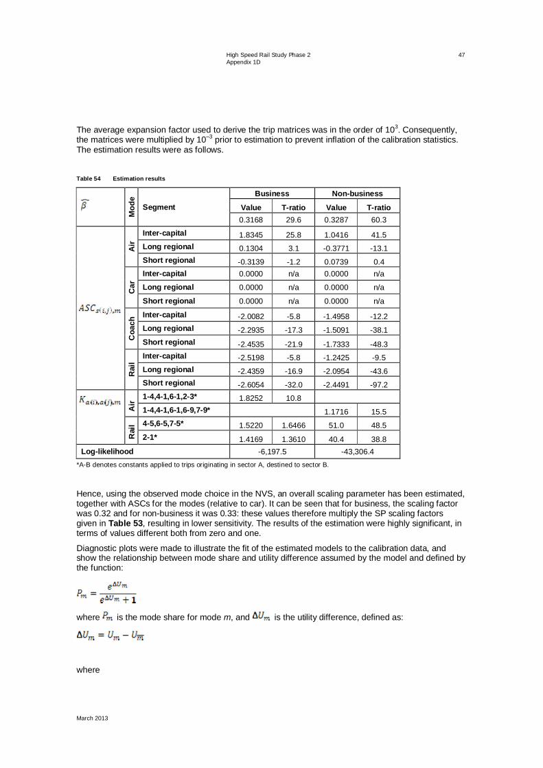
High Speed Rail Study Phase 2 Appendix 1D
March 2013
47
The average expansion factor used to derive the trip matrices was in the order of 103. Consequently, the matrices were multiplied by 10–3 prior to estimation to prevent inflation of the calibration statistics. The estimation results were as follows.
Table 54 Estimation results
Mod
e
Segment Business Non-business
Value T-ratio Value T-ratio 0.3168 29.6 0.3287 60.3
A
ir
Inter-capital 1.8345 25.8 1.0416 41.5 Long regional 0.1304 3.1 -0.3771 -13.1 Short regional -0.3139 -1.2 0.0739 0.4
Car
Inter-capital 0.0000 n/a 0.0000 n/a
Long regional 0.0000 n/a 0.0000 n/a
Short regional 0.0000 n/a 0.0000 n/a
Coa
ch Inter-capital -2.0082 -5.8 -1.4958 -12.2
Long regional -2.2935 -17.3 -1.5091 -38.1 Short regional -2.4535 -21.9 -1.7333 -48.3
Rai
l
Inter-capital -2.5198 -5.8 -1.2425 -9.5 Long regional -2.4359 -16.9 -2.0954 -43.6 Short regional -2.6054 -32.0 -2.4491 -97.2
A
ir
1-4,4-1,6-1,2-3* 1.8252 10.8 1-4,4-1,6-1,6-9,7-9* 1.1716 15.5
Rai
l 4-5,6-5,7-5* 1.5220 1.6466 51.0 48.5 2-1* 1.4169 1.3610 40.4 38.8
Log-likelihood -6,197.5 -43,306.4 *A-B denotes constants applied to trips originating in sector A, destined to sector B.
Hence, using the observed mode choice in the NVS, an overall scaling parameter has been estimated, together with ASCs for the modes (relative to car). It can be seen that for business, the scaling factor was 0.32 and for non-business it was 0.33: these values therefore multiply the SP scaling factors given in Table 53, resulting in lower sensitivity. The results of the estimation were highly significant, in terms of values different both from zero and one.
Diagnostic plots were made to illustrate the fit of the estimated models to the calibration data, and show the relationship between mode share and utility difference assumed by the model and defined by the function:
where is the mode share for mode m, and is the utility difference, defined as:
where

High Speed Rail Study Phase 2 Appendix 1D
March 2013
48
is the composite cost of modes other than m.
The diagnostic plots that follow illustrate the extremely good fit of the estimated models to the calibration data. The dashed line in each figure defines the relationship between mode share and the utility difference between that mode of transport and (the composite of) the others. Data points (i.e. circles) denote the aggregated observed data, the size of each data point being proportional to the number of trips it represents.
Figure 10 Observed air mode shares for business travel plotted against the model estimate

High Speed Rail Study Phase 2 Appendix 1D
March 2013
49
Figure 11 Observed car mode shares for business travel plotted against the model estimate
Figure 12 Observed coach mode shares for business travel plotted against the model estimate

High Speed Rail Study Phase 2 Appendix 1D
March 2013
50
Figure 13 Observed rail mode shares for business travel plotted against the model estimate
Figure 14 Observed air mode shares for non-business travel plotted against the model estimate

High Speed Rail Study Phase 2 Appendix 1D
March 2013
51
Figure 15 Observed car mode shares for non-business travel plotted against the model estimate
Figure 16 Observed coach mode shares for non-business travel plotted against the model estimate

High Speed Rail Study Phase 2 Appendix 1D
March 2013
52
Figure 17 Observed rail mode shares for non-business travel plotted against the model estimate
In addition, an attempt was made to carry out a similar estimation using the RP data from the SP survey. Based on Table 10, of those who claimed to have some choice (820), car was available to 754, air to 579 and rail to 461. The choice proportions were, respectively, 75 per cent, 37 per cent and eight per cent (as a percentage of availability). An overall scaling parameter of 0.25 was estimated. Although this is considered much less reliable than the NVS estimation, it does confirm that the multiplier is considerably less than one.
6.0 Conclusions The resulting demand model has been implemented and it has been concluded that it gives stable and convincing mode share estimates.
Overall, the SP has been successful. Although the results for the generalised cost weights were not considered sufficiently convincing to make the case for departing from the received wisdom incorporated in the model, it has been confirmed that, apart from the ASCs, the general modelling results are not affected by constraining them. Plausible VoTs have been derived and, although the higher values for long regional relative to inter-capital were unexpected, they are well supported in the SP analysis.
After examining ASCs for HSR, it has been concluded that the existing assumptions, of no difference between air and HSR for inter-capital and long regional, and of no difference between rail and HSR for short regional, are confirmed for business. For non-business there is a definite indication that HSR might be more positively viewed, with an advantage in favour of HSR of 45-55 minutes.
The structure of the existing demand model has been confirmed.
Overall, the SP has delivered a more robust demand model, as well as providing a substantial database which could be further analysed for more detailed segmentation.
In addition to the technical results produced from the SP, the survey itself provided a number of useful indications of the likely response to an HSR line. Interest among respondents was generally favourable, and indeed this assisted in cooperation with the survey. In both the pilot and the main

High Speed Rail Study Phase 2 Appendix 1D
March 2013
53
survey there was strong support for HSR, and many respondents chose HSR in all scenarios presented, while some of those who never chose it still said that they would consider it for other journeys. Rail passengers were most likely to switch to HSR, followed by air. As expected, there was less response from existing car travellers, many of whom will have reasons other than time and cost for choosing the car mode.
The general impression was that HSR was seen as a good choice for journeys to the large centres such as Melbourne, Brisbane and the Gold Coast, while those living in the regional areas were, if anything, more enthusiastic. For those living in the major cities there was a strong impression that central stations were preferred to peripheral locations, especially those that did not have both good public transport and parking available (such as Parramatta in Sydney). This was less of an issue for those living in the regional areas.

High Speed Rail Study Phase 2
Department of Infrastructure and Transport March 2013
Appendix 1E Demand forecasting procedures
High Speed Rail Study Phase 2 Appendix 1E
March 2013
Appendix 1E Demand forecasting procedures
Prepared for
Department of Infrastructure and Transport
Prepared by AECOM Australia Pty Ltd Level 21, 420 George Street, Sydney NSW 2000, PO Box Q410, QVB Post Office NSW 1230, Australia T +61 2 8934 0000 F +61 2 8934 0001 www.aecom.com ABN 20 093 846 925
March 2013
AECOM in Australia and New Zealand is certified to the latest version of ISO9001 and ISO14001.
© AECOM Australia Pty Ltd (AECOM). All rights reserved.
In accordance with the east coast high speed rail (HSR) study terms of reference, AECOM and its sub-consultants (Grimshaw, KPMG, SKM, ACIL Tasman, Booz & Co and Hyder, hereafter referred to collectively as the Study Team) have prepared this report (Report). The Study Team has prepared this Report for the sole use of the Commonwealth Government: Department of Infrastructure and Transport (Client) and for a specific purpose, each as expressly stated in the Report. No other party should rely on this Report or the information contain in it without the prior written consent of the Study Team. The Study Team undertakes no duty, nor accepts any responsibility or liability, to any third party who may rely upon or use this Report. The Study Team has prepared this Report based on the Client's description of its requirements, exercising the degree of skill, care and diligence expected of a consultant performing the same or similar services for the same or similar study, and having regard to assumptions that the Study Team can reasonably be expected to make in accordance with sound professional principles. The Study Team may also have relied upon information provided by the Client and other third parties to prepare this Report, some of which may not have been verified or checked for accuracy, adequacy or completeness. The Report must not be modified or adapted in any way and may be transmitted, reproduced or disseminated only in its entirety. Any third party that receives this Report, by their acceptance or use of it, releases the Study Team and its related entities from any liability for direct, indirect, consequential or special loss or damage whether arising in contract, warranty, express or implied, tort or otherwise, and irrespective of fault, negligence and strict liability. The projections, estimation of capital and operational costs, assumptions, methodologies and other information in this Report have been developed by the Study Team from its independent research effort, general knowledge of the industry and consultations with various third parties (Information Providers) to produce the Report and arrive at its conclusions. The Study Team has not verified information provided by the Information Providers (unless specifically noted otherwise) and it assumes no responsibility nor makes any representations with respect to the adequacy, accuracy or completeness of such information. No responsibility is assumed for inaccuracies in reporting by Information Providers including, without limitation, inaccuracies in any other data source whether provided in writing or orally used in preparing or presenting the Report. In addition, the Report is based upon information that was obtained on or before the date in which the Report was prepared. Circumstances and events may occur following the date on which such information was obtained that are beyond the Study Team's control and which may affect the findings or projections contained in the Report, including but not limited to changes in 'external' factors such as changes in government policy; changes in law; fluctuations in market conditions, needs and behaviour; the pricing of carbon, fuel, products, materials, equipment, services and labour; financing options; alternate modes of transport or construction of other means of transport; population growth or decline; or changes in the Client's needs and requirements affecting the development of the project. The Study Team may not be held responsible or liable for such circumstances or events and specifically disclaim any responsibility therefore.

High Speed Rail Study Phase 2 Appendix 1E
March 2013
Quality information Document Appendix 1E
Ref 60238250-1.0-REP-0101–1E
Date March 2013

High Speed Rail Study Phase 2 Appendix 1E
March 2013
Table of contents 1.0 Introduction and objectives 1 2.0 Model zone system and transport level-of-service 2 3.0 Base market 3 4.0 Market projections 3
4.1 Background 3 4.2 Air travel trends in the corridor 4 4.3 Rail travel trends in the corridor 6 4.4 Analysis of traffic trends in the corridor 7 4.5 Conclusions on income elasticities 10
5.0 Demand forecasting procedures 11 5.1 Overview 11 5.2 Incorporating the stated preference survey conclusions 12 5.3 Metropolitan station choice and access mode 13 5.4 HSR service mix 14
6.0 Model outputs 16 6.1 Output templates 16 6.2 Key formulae 16 6.3 Ramp-up of demand 17
7.0 Performance of the demand forecasting procedures 19 7.1 Introduction and objectives 19 7.2 Implications of the revised projections 19 7.3 The performance of the access/egress and station choice models 20 7.4 Elasticities of demand 23 7.5 Consistency with international experience 23
7.5.1 Scope 23 7.5.2 The split between air and HSR 23 7.5.3 The diversion from car and induced travel 25 7.5.4 Shares by trip length 28
7.6 Comparisons with previous local studies 30

High Speed Rail Study Phase 2 Appendix 1E
March 2013
1
1.0 Introduction and objectives The multi-modal transport model for the east coast corridor is designed to estimate demand, revenues and user benefits for High Speed Rail (HSR) system alternatives and to assess the impacts of changes in the key attributes of HSR transport products and competing transport modes.
For phase 1, a strategic forecasting approach (Figure 1) was designed to answer the key demand questions concerning the nature of the current markets in the Brisbane-Sydney-Melbourne east coast corridor, how they will grow in future, the potential for diversion to HSR and the extent to which HSR may stimulate demand.
The logic of this approach was also adopted in the previous Australian HSR studies, such as the Very Fast Train Study1 and Speedrail2. Figure 1 Structure of demand forecasting for the east coast corridor
Estimates of the current market size and mode shares were derived from the National Visitors Survey (NVS)3 over an 11 year period between 2000 and 2010.
Travel demand growth was then projected as a function of the future population growth projections in the corridor and income growth, based on techniques used by the Bureau of Infrastructure, Transport and Regional Economics (BITRE). In order to estimate the diversion to the proposed new HSR services and the induced travel brought about by the consequent improvements in accessibility, models of mode choice and induced travel were developed based on a combination of international and local experience and evidence.
This process has been further developed for phase 2, and the principal changes which have been incorporated in this demand forecasting procedure are summarised in Table 1.
1VFT: Access Economics, Cost benefit study of the Very Fast Train Project, 1990. Arup and TMG, East Coast Very High Speed Train Scoping Study, Phase 1 Preliminary Study Final Report, 2001. 2 SKM & MVA, Speedrail Patronage and Revenue Forecasts, supplement to final report, 1999. 3 Tourism Research Australia, National Visitors Survey.
Es ta bl i sh the s ize of a l l the re levant ma rkets and the current mode s ha res
Interci ty a nd regiona l ma rkets, between Mel bourne a nd Bris ba ne for car, train, ai r a nd coach
Foreca s t the growth in thes e ma rkets For ea ch future scena rio to 2035, 2050 and 2065
HSR Service
Forecast the divers ion to HSR and induced tra vel demands
For ea ch mode in each ma rket
Outputs to appra is a lsHSR patronage, revenues and us er benefi ts , a nd other required outputs

High Speed Rail Study Phase 2 Appendix 1E
March 2013
2
Table 1 Model enhancements
Module Enhancements to the specification
Study area, zone system and level of transport service
A more detailed zone system in the phase 2 study area and improvements to the transport level-of-service data.
Base market Incorporation of the improved base market estimates described in Appendix 1B.
Market projections Incorporation of the findings of a review of the elasticity of light vehicle travel growth to income by BITRE (Appendix 1H).
The mode choice model
Incorporation of the findings of a major stated preference (SP) survey in the corridor (Appendix 1D). Development of the demand model on the updated base market data. An extended demand model structure, incorporating a more detailed station and airport access methodology and new procedures for representing a mix of HSR services.
Model outputs Factors for patronage ramp-up after opening. An extended output template.
2.0 Model zone system and transport level-of-service Within the phase 2 study area, the zone system (Figure 2) comprises 167 internal zones, and there are 11 external zones, which represents a doubling of the number of zones from phase 1. In metropolitan areas, zone sizes have been selected to enable differentiation between the potential HSR station locations. Outside the state capital areas, further refinements have been made affecting Wollongong, Wagga Wagga, Gold Coast and Newcastle.
Transport level-of-service data (Table 2) was assembled for the base year (2009) in phase 1 from timetables, maps and other sources.
This data has been audited and generally enhanced for the new zone system. Specific tasks undertaken include:
Establishing transport level-of-service data for the refined zone system.
Incorporation of metropolitan transport level-of-service data from the state transport models.
Incorporation of road journey time information derived from the corridor registration number survey.
Expansion of the coverage of the air services to regional areas.
Incorporation of additional information on air fares. Table 2 Level of service data specification
Mode Level of service characteristics in the model
Air In-vehicle time, service frequency, access/egress, check-in time, fare.
HSR In-vehicle time, service frequency, fare, interchange, access/egress.
Bus, coach and conventional rail In-vehicle time, service frequency, fare, access/egress.
Car In-vehicle time, vehicle operating cost.

High Speed Rail Study Phase 2 Appendix 1E
March 2013
3
Figure 2 Zone system
The smaller figures on the left and right show in greater detail the zones in areas of greater residential density.
3.0 Base market The updated base market described in Appendix 1B has been incorporated in the model.
4.0 Market projections
4.1 Background The increase in future travel demand is expected to be driven by two main factors: population growth and economic growth. Improvements in transport accessibility are a third influence on the travel demands for each mode. For phase 1, the future demand forecasting methodology was based on techniques used by BITRE4, supplemented by analysis of corridor aviation demands and the evidence of previous demand studies5.
The formulation is an elasticity model sensitive to the trip origin and destination populations and income (as measured by Gross Domestic Product (GDP)/capita). The further influence of transport accessibility and prices (the generalised cost of travel by each mode) on the balance of overall travel demand between the transport modes is derived from the induced travel demand model (Section 1.5).
Concerning the income elasticities used in this model, the following sections describe the evidence for each transport mode.
4 BITRE, National road network intercity traffic projections to 2030, WP71, 2009. 5 Speedrail, op. cit.

High Speed Rail Study Phase 2 Appendix 1E
March 2013
4
4.2 Air travel trends in the corridor Through an analysis of past trends in aviation demand between 1994 and 2010 in the east coast corridor6, the elasticity of aviation demand to income has been verified. This was a period of considerable change in the Australian (and global) aviation industry, with such notable events as:
2000 – Virgin Blue launched.
2001 – Collapse of Ansett.
2001 – World Trade Centre terrorist attack (9/11).
2002 – Bali bombings.
2003 – SARS outbreak.
2003 – Qantas established low cost subsidiary Jetstar.
2006 – Australian Airlines ceased operation.
2007 – Tiger Airways commenced in Australia.
A model of aviation demand was fitted to the trends in air travel. The model uses an income elasticity of +1.0 and an air fare elasticity of -0.3, consistent with the expected demand elasticities. The fit of this model to the past trends in air travel is summarised in Figure 3 to Figure 5.
For the major routes in the study area, the model predicts the trend in aggregate demand well (Figure 3). Smaller routes (i.e. less than one million air passengers per year) have been pooled into three categories (Figure 4 and Figure 5):
Established minor routes (e.g. Canberra-Sydney and Canberra-Brisbane).
New minor routes (e.g. Sunshine Coast routes).
Regional routes (e.g. Albury-Wodonga, Wagga Wagga, Dubbo, Coffs Harbour, Port Macquarie and Ballina).
Regional route data prior to 2005 is not included in this analysis due to significant changes in service patterns caused by the collapse of airlines in the period of 2001 to 2003. While there were variations in the trends between the individual routes, it is clear that the model is effective at predicting the aggregate trends across the three categories of smaller routes listed above.
It is concluded that aviation models incorporating GDP/capita elasticity values of +1.0 fit the trends in air travel for the east coast routes affected by the proposed HSR service. This elasticity is broadly consistent with the Sydney Aviation Capacity Study (which quotes a range for domestic travel of +0.4 to +1.2)7.
6 BITRE Aviation Statistics Data: Domestic Airline Activity, Domestic Totals and Top Routes, regular publication. 7 ibid.

High Speed Rail Study Phase 2 Appendix 1E
March 2013
5
Figure 3 Comparison of a model back-forecast with air travel trends, 1994-2010: total of major routes
Figure 4 Comparison of a model back-forecast with air travel trends, 1994-2010: minor routes
0.0
5.0
10.0
15.0
20.0
25.0
1994 1995 1996 1997 1998 1999 2000 2001 2002 2003 2004 2005 2006 2007 2008 2009 2010
Ann
nual
air
pas
seng
er d
eman
d (m
illio
ns)
Calendar year
Major Routes Actual Major Route Modelled
0.0
0.2
0.4
0.6
0.8
1.0
1.2
1.4
1.6
1.8
2.0
1994 1995 1996 1997 1998 1999 2000 2001 2002 2003 2004 2005 2006 2007 2008 2009 2010
Ann
nual
air
pass
enge
r dem
and
(mill
ions
)
Calendar year
Esablished minor Actual Recent minor Actual
Esablished minor Modelled Recent minor Modelled
Established Minor Actual
Established Minor Modelled
Recent Minor Actual
Recent Minor Modelled

High Speed Rail Study Phase 2 Appendix 1E
March 2013
6
Figure 5 Comparison of a model back-forecast with air travel trends, 2005-2010: regional routes
4.3 Rail travel trends in the corridor The evidence on rail travel demand from ticketing data for long distance rail travel (Figure 6 and Figure 7) shows no overall growth over the past decade in the XPT Sydney-Melbourne train service and no growth in the period 2006-2009 in other parts of the east coast corridor. However, the XPT trend suggests that it may have been affected by the introduction of low cost airline services and that it would be inappropriate to conclude that the income elasticity is insignificant, especially as there appears to have been a general return to patronage growth in recent years.
With this background, it has been preferred to use the relatively low income elasticity (+0.57) established in the Speedrail study. This income elasticity has also been used for coach travel. Figure 6 Ten-year trend in Sydney-Melbourne XPT patronage
0.0
0.5
1.0
1.5
2.0
2.5
2005 2006 2007 2008 2009 2010
Ann
nual
air
pas
seng
er d
eman
d (m
illio
ns)
Calendar year
Regional Modelled Regional Actual
050000
100000150000200000250000300000350000400000450000
Annu
al p
atro
nage
Year
Total XPT Patronage

High Speed Rail Study Phase 2 Appendix 1E
March 2013
7
Figure 7 Three-year trends in other regional rail services
4.4 Analysis of traffic trends in the corridor Diverted car travel is an important component of the HSR demand forecasts, but there is uncertainty regarding the future rates of car travel growth.
An initial analysis of car travel trends in the NVS data over the period 2000-2011 did not suggest that there had been major growth in car travel in the corridor and a recent independent report by Tourism Research Australia8 suggested that car travel for holidays was reducing in Australia as people choose more overseas holidays. International advisors confirmed that the projection of car travel demand is also a concern in the forecasts for High Speed 2 in the United Kingdom.
Clarification of the issue was sought through an analysis of the trends in light vehicle traffic flow on the major inter-capital highways in the corridor. BITRE analysed the trends in light vehicle traffic volumes at 56 sites (Figure 8 and Figure 9) on the Hume Highway and Pacific Highway over the two decades to 2011 (refer to Appendix 1H for a detailed description of this work).
8 Tourism Research Australia, What is driving Australians’ travel choices?, 2011.

High Speed Rail Study Phase 2 Appendix 1E
March 2013
8
Figure 8 Victorian traffic count site locations
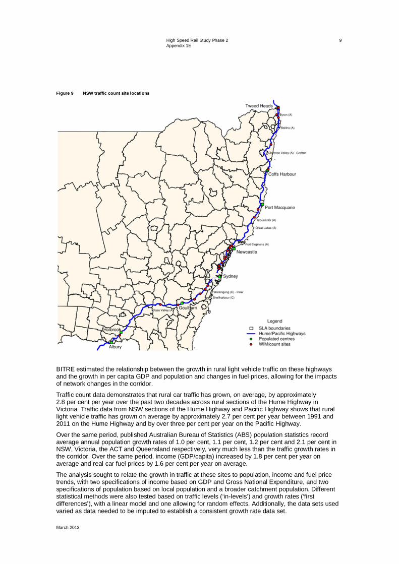
High Speed Rail Study Phase 2 Appendix 1E
March 2013
9
Figure 9 NSW traffic count site locations
BITRE estimated the relationship between the growth in rural light vehicle traffic on these highways and the growth in per capita GDP and population and changes in fuel prices, allowing for the impacts of network changes in the corridor.
Traffic count data demonstrates that rural car traffic has grown, on average, by approximately 2.8 per cent per year over the past two decades across rural sections of the Hume Highway in Victoria. Traffic data from NSW sections of the Hume Highway and Pacific Highway shows that rural light vehicle traffic has grown on average by approximately 2.7 per cent per year between 1991 and 2011 on the Hume Highway and by over three per cent per year on the Pacific Highway.
Over the same period, published Australian Bureau of Statistics (ABS) population statistics record average annual population growth rates of 1.0 per cent, 1.1 per cent, 1.2 per cent and 2.1 per cent in NSW, Victoria, the ACT and Queensland respectively, very much less than the traffic growth rates in the corridor. Over the same period, income (GDP/capita) increased by 1.8 per cent per year on average and real car fuel prices by 1.6 per cent per year on average.
The analysis sought to relate the growth in traffic at these sites to population, income and fuel price trends, with two specifications of income based on GDP and Gross National Expenditure, and two specifications of population based on local population and a broader catchment population. Different statistical methods were also tested based on traffic levels (‘in-levels’) and growth rates (‘first differences’), with a linear model and one allowing for random effects. Additionally, the data sets used varied as data needed to be imputed to establish a consistent growth rate data set.

High Speed Rail Study Phase 2 Appendix 1E
March 2013
10
The statistical models were all inelastic to fuel prices, with the most common range being -0.1 to -0.2.
Using the raw traffic count data, the simple ‘in-levels’ models imply a statistically significant and positive income elasticity for rural light vehicle traffic across all three sections. The Victorian Hume Highway data implies an average income elasticity for light vehicle rural traffic volumes of +0.5 to +0.8, depending on the estimation method used. Statistically, the elasticity is significantly less than one. The NSW Hume Highway and Pacific Highway data implies an average income elasticity of around +1.2 for these sections.
Assigning missing traffic count data and estimating the relationship using the annual change in light vehicle traffic volumes appears to imply broadly similar long-run elasticities. The results show that light vehicle traffic growth has a statistically significant and positive correlation with income, with income elasticity at around +0.5 to +0.8 across Victorian sections of the Hume Highway, and at +1.1 on NSW sections of the Hume Highway and possibly higher on the Pacific Highway.
The difference in the measured income elasticity across the Victorian and NSW count sites could be influenced by differences in the relative distribution of count site locations across each section, unaccounted-for network changes and differences in the relative composition of trip types across the two road sections9.
Having considered all of the modelling results and recognising the weakness of some of the statistical models relating to shortcomings in the data, the analysis confirms that car travel demand grows significantly with income. It is concluded that, for the purposes of this study, an income elasticity of +0.8 should be assumed, while a more conservative assumption for shorter journeys would be appropriate.
4.5 Conclusions on income elasticities The values on which the demand forecasting is based are given in Table 3. The air, coach and rail elasticities derive from phase 1, as described above. The car elasticities derive from the BITRE analysis. Both the car and air elasticities have been adjusted downwards slightly to ensure that there is no duplication of the income effect with the mode choice/induced travel model. For short regional journeys, the nominal elasticities have been halved as described above.
The elasticities are assumed to mature through time, the maturity rate for air being consistent with the aviation capacity study data10. For car, coach and rail, a faster maturation rate has been used, as a conservative assumption. Table 3 Travel demand elasticities to income growth
Year Air
Car Rail/coach Inter-
capital/long regional
Short regionalInter-
capital/long regional
Short regional
2009 1.0 0.8 0.4 0.57 0.28
2035 0.88 0.62 0.31 0.44 0.22
2050 0.82 0.54 0.27 0.38 0.19
2065 0.76 0.46 0.22 0.33 0.16
Finally, it is expected that the distribution of employment within metropolitan areas could have an effect on HSR demand separate from that of population, particularly for business travel. However, as the states’ employment distribution projections for the three metropolitan areas do not change significantly in the future, this factor can be ignored in the projections (because of its stability through time).
9 The Victorian data includes count sites spread across the entire length of the Hume Highway, whereas most of the count sites on the Hume Highway and Pacific Highway in NSW are located within 200 kilometres of Sydney. 10 Australian and NSW governments, Joint study on aviation capacity in the Sydney region, 2012.

High Speed Rail Study Phase 2 Appendix 1E
March 2013
11
5.0 Demand forecasting procedures
5.1 Overview The structure of the demand forecasting procedures is illustrated in Figure 10, with the additional components incorporated in phase 2 highlighted in red. Figure 10 Extended model structure
The impacts of HSR in the east coast corridor would be twofold: a transfer of demand from existing modes to HSR and an overall increase in travel demand caused by the improved accessibility (referred to as induced demand). Although improved accessibility is also likely to affect the nature and rate of development in the corridor, this has not been taken into account in the forecasts.
The demand forecasting procedures forecast the amount of transfer from other modes to HSR using a model of transport mode choice, called a ‘hierarchical logit’ model. The model has been extended to include a forecast of the additional travel induced by HSR.
The model distinguishes between business and non-business travel, reflecting their different patterns, modal preferences and cost sensitivities. The structure of the model has been derived from existing models and transport research, both Australian and international.
The mode share model forecasts the amount of diversion from the existing modes to the HSR service in relation to the comparative levels of service and the relative travel costs (fares or vehicle operating costs). Changes in journey times, service frequencies, ease of access to rail stations and airports and the fares or operating costs all influence the amount of mode shift to HSR. The results of the SP survey, described in Appendix 1D, have been incorporated in this component of the model.
The pattern of train services along the line is a consideration. There would be a mixture of stopping, limited stop and non-stop services. The demand forecasting procedures have been developed to enable passenger demands to be appropriately allocated across the different services as well as ensure that the attractiveness to passengers of a mix of services is appropriately reflected in the HSR demand forecasts.
Car Fast mass transport coach/ standard rail
HSR Service mix HSR Air
Metropolitan station choice
station access mode
Stated preference survey
Base and induced travel

High Speed Rail Study Phase 2 Appendix 1E
March 2013
12
In the cities, there are decisions to be made on central station locations and peripheral ‘park and ride’ stations. Station design concepts need to provide appropriate numbers of parking spaces. For these reasons, the forecasting procedures included specific detail on the choice of mode by HSR passengers for accessing stations and their choice of station. For egress at the destination, the model chooses the most accessible stations, allowing for the egress modes available.
5.2 Incorporating the stated preference survey conclusions Various standard parameter values have been updated in the model based on the results of the SP survey (Table 4 and Table 5). The most important changes are to the values of time, which are those estimated from the SP survey. Additional minor changes have been made to average group sizes and average parking durations (based on the average length of visit).
The waiting time parameter accords with established practice. Vehicle operating costs represent the perceived component of costs. For non-business travel this is fuel plus parking costs. The estimates were based on the ABS Survey of Motor Vehicle Usage (for average fuel consumption) and average fuel prices sourced from the Australian Institute of Petroleum. The values assume that businesses perceive the full resource cost of operating a vehicle.
Daily parking costs are assumed in 2009. The high cost is applied to metropolitan airport long-term parking, medium costs to Canberra Airport and low costs to peripheral HSR station parking. Parking charges are not applied at regional HSR stations. Table 4 Values of time and other parameters: phase 2
Parameters Market Unit Business Non-business
2009 value of time ($2012)
Inter-capital $/hr 57 14
Long regional $/hr 81 20
Short regional $/hr 38 9.5
Waiting time factor All - 2.0 Table 5 Values of time and other parameters: phase 2
Parameters Market Unit Business Non-business
2009 parking charges ($2012 per day)
High $ 48 21
Medium $ 21 16
Low $ 24 10.50
Group size All People 1.4 2.4
Parking duration All Days 2.0 3.6
Vehicle operating costs ($2012) All Cents/km 31.2 15.5
Air check-in time All Mins 45
HSR interchange penalty All Mins 20
The key parameters for the hierarchical logit model structure have been determined directly from the findings of the SP survey, or adjusted in relation to those estimates. In this structure, the scaling parameters for the choice between the existing modes of transport were taken from the SP model and then re-scaled to the NVS data as described in Appendix 1D. These are the ‘second level’ parameters in Table 6, covering the choice between car, fast mass transport and coach/standard rail.
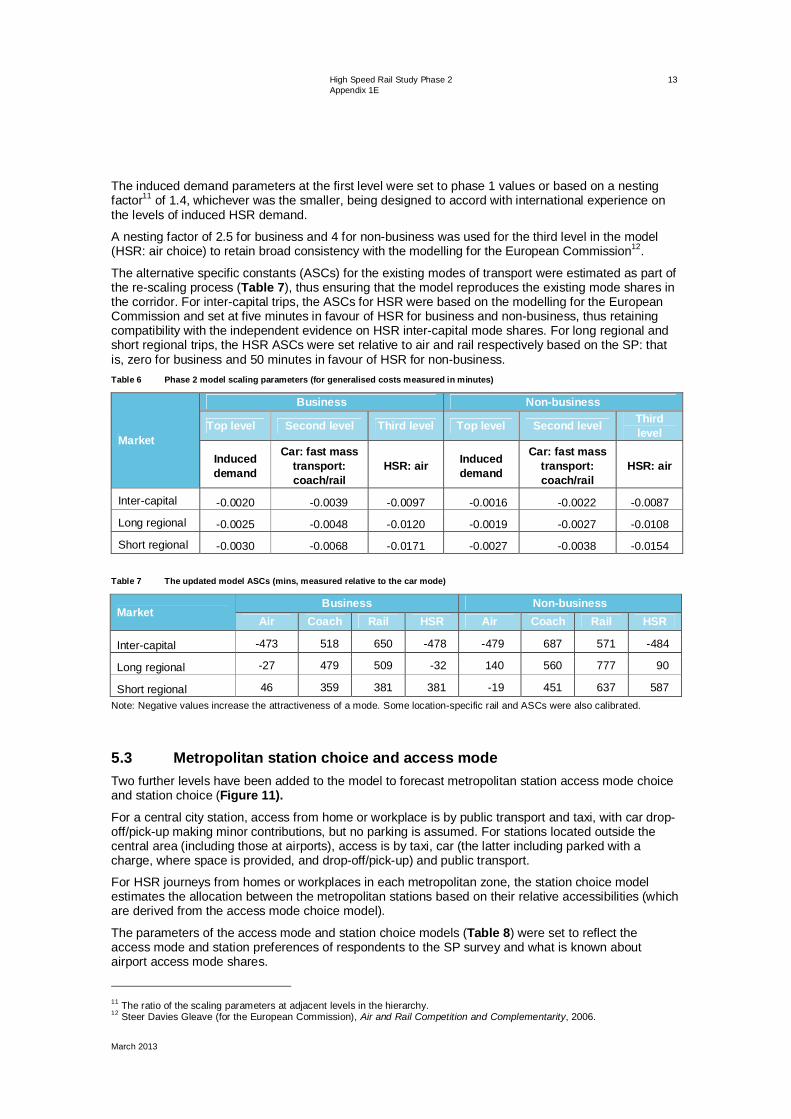
High Speed Rail Study Phase 2 Appendix 1E
March 2013
13
The induced demand parameters at the first level were set to phase 1 values or based on a nesting factor11 of 1.4, whichever was the smaller, being designed to accord with international experience on the levels of induced HSR demand.
A nesting factor of 2.5 for business and 4 for non-business was used for the third level in the model (HSR: air choice) to retain broad consistency with the modelling for the European Commission12.
The alternative specific constants (ASCs) for the existing modes of transport were estimated as part of the re-scaling process (Table 7), thus ensuring that the model reproduces the existing mode shares in the corridor. For inter-capital trips, the ASCs for HSR were based on the modelling for the European Commission and set at five minutes in favour of HSR for business and non-business, thus retaining compatibility with the independent evidence on HSR inter-capital mode shares. For long regional and short regional trips, the HSR ASCs were set relative to air and rail respectively based on the SP: that is, zero for business and 50 minutes in favour of HSR for non-business. Table 6 Phase 2 model scaling parameters (for generalised costs measured in minutes)
Market
Business Non-business
Top level Second level Third level Top level Second level Third level
Induced demand
Car: fast mass transport: coach/rail
HSR: air Induced demand
Car: fast mass transport: coach/rail
HSR: air
Inter-capital -0.0020 -0.0039 -0.0097 -0.0016 -0.0022 -0.0087
Long regional -0.0025 -0.0048 -0.0120 -0.0019 -0.0027 -0.0108
Short regional -0.0030 -0.0068 -0.0171 -0.0027 -0.0038 -0.0154 Table 7 The updated model ASCs (mins, measured relative to the car mode)
Market Business Non-business
Air Coach Rail HSR Air Coach Rail HSR
Inter-capital -473 518 650 -478 -479 687 571 -484
Long regional -27 479 509 -32 140 560 777 90
Short regional 46 359 381 381 -19 451 637 587 Note: Negative values increase the attractiveness of a mode. Some location-specific rail and ASCs were also calibrated.
5.3 Metropolitan station choice and access mode Two further levels have been added to the model to forecast metropolitan station access mode choice and station choice (Figure 11).
For a central city station, access from home or workplace is by public transport and taxi, with car drop-off/pick-up making minor contributions, but no parking is assumed. For stations located outside the central area (including those at airports), access is by taxi, car (the latter including parked with a charge, where space is provided, and drop-off/pick-up) and public transport.
For HSR journeys from homes or workplaces in each metropolitan zone, the station choice model estimates the allocation between the metropolitan stations based on their relative accessibilities (which are derived from the access mode choice model).
The parameters of the access mode and station choice models (Table 8) were set to reflect the access mode and station preferences of respondents to the SP survey and what is known about airport access mode shares.
11 The ratio of the scaling parameters at adjacent levels in the hierarchy. 12 Steer Davies Gleave (for the European Commission), Air and Rail Competition and Complementarity, 2006.

High Speed Rail Study Phase 2 Appendix 1E
March 2013
14
Figure 11 Station choice model structure including access modes
Table 8 Station and access mode choice parameters
Parameter Taxi Parked car*
Pick up/ drop off
Public transport Metropolitan
CBD HSR station
Other metropolitan HSR station
Airport stations
Pick up/drop off time weight - - 2 -
Access journey time weight 2.0
ASC (mins) - 40 20 -70 -30 -10
Scaling of station/ Mode choice -0.025/-0.05
*Parked car is assumed to be unavailable to visitors.
5.4 HSR service mix This new sub-model allocates HSR passengers between the services available for their journey based on the comparative journey times and service frequencies. It also calculates a measure of the overall attractiveness of the mix of available services, on which the forecasts of diversion to HSR are based.
The approach to allocating passengers between a mix of HSR services draws on the Rooftop model concept developed in the United Kingdom13, which has also been applied in Australia on detailed train service studies (such as Victorian Regional Fast Rail).
The Rooftop model forecasts passenger preferences between differently-timed train services using a time profile of passenger demand through the day. As such, detail is not available for the high speed forecasts, and is not relevant when forecasting 20-50 years ahead. A simplified procedure has been developed which simulates the behaviour of the Rooftop model.
The following process is applied for each pair of stations on the HSR network.
If more than one service provides for HSR journeys between a pair of stations, the quickest HSR service is taken as the reference service and defined as ‘service 1’. This service has frequency f1.
If any other service takes the same time as the reference service, then the journeys between the pair of stations are simply shared between the two services in proportion to their respective frequencies. If the other service is slower then, using the same allocation process, it is allocated a smaller share of the journeys by reducing its service frequency. The amount of the frequency reduction is proportional to the extra journey time over the reference service.
13 Passenger Demand Forecasting Handbook, Version 5, Association of Train Operating Companies, 2009.
CBD Station Peripheral Station
Pick up/drop off Public transport Taxi Parked car Pick up/drop off Public transport Taxi

High Speed Rail Study Phase 2 Appendix 1E
March 2013
15
The frequencies of the slower services are reduced by a factor (fitted to reproduce the Rooftop model) to reflect the lower attractiveness of their longer journey times:
fs’ = fs * (1-4.8*ts/(60/f1)) for s>1
where:
fs’ is the modified value of fs for service s
ts is the excess journey time over service 1
and if the frequency factor is less than 0 it is reset to 0.
The HSR demand between each pair of stations is allocated to each service in proportion to these modified frequencies.
The forecasts of the demand model are based on the characteristics of the fastest service (service 1) but with its service frequency increased to allow for the additional slower services, based on their modified frequencies:
f1’ = f1 + s>1 fs * (1-4.8*ts/(60/f1))
Comparisons of the results of this formula against a Rooftop model simulation for three competing services in Figure 12 demonstrate the reasonable match.
Tests of the effects of this process on the HSR service gave the following illustrative forecasts:
Two different services link Melbourne and Canberra. Both have the same journey time, but one has twice the service frequency; the more frequent service is allocated 67 per cent of the passenger demand.
In another test of the same service pattern, but with identical frequencies, the passenger demand is split equally between the two services.
There are two services between Newcastle and Brisbane, of which one is 10 minutes faster and has twice the frequency; this is allocated all of the passenger demand.
Figure 12 Comparison of the share of passengers between three HSR services for the service mix model and the Rooftop model
0%
10%
20%
30%
40%
50%
60%
70%
80%
90%
100%
0% 10% 20% 30% 40% 50% 60% 70% 80% 90% 100%
Mod
elle
d se
rvic
e sh
ares
(%
)
Simulated Rooftop Shares
Service 1
Service 2
Service 3

High Speed Rail Study Phase 2 Appendix 1E
March 2013
16
6.0 Model outputs
6.1 Output templates The demand forecasting procedures are designed to generate inputs to the commercial performance and economic appraisals for each planning year including passenger demand, fares revenue and transport user benefits.
The model output templates provide both summary and detailed analyses of the model forecasts for all appraisals.
The main templates provide the overall summaries by trip purpose and 10x10 sector breakdowns of: Total corridor demand with and without HSR.
HSR trips, passenger kilometres and revenues.
Reductions in air, rail and coach revenues.
Road vehicle kilometres.
The overall user benefits by purpose in minutes and dollars.
The resource cost adjustment for unperceived vehicle operating costs.
An estimate of the overall metropolitan road decongestion benefits arising from HSR.
Number of HSR passengers who access HSR by park and ride and the parking revenues.
The station access template provides statistics on the modes of access to every HSR station.
The services outputs template gives the station-to-station matrix of travel demand by purpose for every HSR service, identifying interchanging passengers.
The service mix template gives passenger loadings along the line for each service and the boardings/alightings at every HSR station.
The financial matrices template provides a number of the main outputs on a grouped station-to-station basis for input to the financial modelling used in the appraisal of commercial performance.
The economics template provides detailed economic data for every cell in the travel demand matrix by purpose, enabling the economic appraisal.
6.2 Key formulae The benefit is measured as the difference between the base ‘overall’ travel cost and the with-HSR ‘overall’ travel cost, where ‘overall’ allows for all the available modes of transport.
The measure of the overall cost is the logsum14. Its general form is: (1/ ) * Ln ( m exp( * generalised costm)
where: is the model parameter
m refers to the set of transport modes
the generalised cost includes in-vehicle time, waiting time, access time, check-in time, fares and out-of-pocket costs; costs are converted to equivalent minutes of in-vehicle time using the model values of time; also included is the alternative specific constant for each mode (from the model)
the logsum is in units of travel time minutes. 14 Rand, Using the Logsum as an Evaluation Measure, Working paper, AVV Transport Research Centre, 2005.

High Speed Rail Study Phase 2 Appendix 1E
March 2013
17
The benefit (ignoring induced travel) is then: Benefit (in minutes) = Total base trips * (logsumbase case – logsumwith-HSR case)
This can be converted to dollars using the appropriate value of time. This formula is extended to include the benefits of induced travel using either the rule of a half or a more accurate method using the following analytical formula15:
Benefit = (Total base trips / ) * {exp[ *(logsumwith-HSR case - logsumbase case)]-1} where is the induced travel parameter.
A resource cost correction is calculated for the unperceived car costs. This is:
RCA*(car distance/group size) * {(total base trips + induced trips)*%carwith-HSR case - total base trips * %carbase case}
where RCA is the resource cost/vehicle kilometre adjustment, different for business and non-business.
Metropolitan road decongestion costs are:
CGC x (car vehicle distancemet areas / group size) * {(total base trips + induced trips) * %carwith-HSR caae - total base trips x %carbase case}
where CGC is congestion cost/kilometre expressed in $ (from the state metropolitan models).
6.3 Ramp-up of demand Following the introduction of new transport infrastructure and services, there is a delay in the level of demand achieving forecast levels as travellers adapt to the availability of a new transport facility. Where the new facility is markedly different to existing transport infrastructure and services, the delay is likely to be longer. The time the travel demands take to build up to the expected levels is referred to as the ramp-up period.
A five year ramp-up profile for the HSR service is presented in Table 9 on the basis of broad assumptions about the lag times for demand build-up as a function of the trip purpose (Table 10). This suggests that 40 per cent of the forecast demand would be expected in the first year after opening.
A review of available information on the ramp-up of transport demand is presented in Table 11. Ramp up on toll roads is typically expected to be achieved within two years and this is reported to be true of some HSR services (e.g. many of the French TGV services). But for other HSR services it has taken longer: the Thalys service between Paris, Brussels, Cologne and Amsterdam and the Tokaido service in Japan are both reported to have achieved ramp-up of demand in five years.
Many European and Japanese HSR services were developed in corridors that already had high levels of rail demand, which likely shortened the ramp-up period significantly. This is not the case along the east coast of Australia. The proposed HSR profile is very similar to that assumed for the Californian High Speed Train. While this is somewhat longer than originally assumed for Speedrail, the demand pattern on the east coast HSR includes longer and less frequent journeys. Table 9 HSR ramp-up assumption
Year after opening
Opening year (1) 2 3 4 5
40% 55% 75% 90% 100%
15 Williams and Moore, ‘On the appraisal of highway investments under fixed and variable demand’, Journal of transport economics and policy, 1990.

High Speed Rail Study Phase 2 Appendix 1E
March 2013
18
Table 10 Ramp-up/lag assumptions by source of HSR travel (the number of years ramp-up for each segment)
Purpose Source of HSR travel
Diverted from air Diverted from other modes Induced
Business 2 3 4
Other 3 4 5 Note: a lag of three years implies that full demand is achieved at the beginning of year four.
Table 11 Ramp-up evidence and assumptions
Sources (reports) Year after opening
Opening year (1) 2 3 4 5
Speedrail
Core 78% 95% 100% 100% 100%
Induced 20% 40% 60% 80% 100%
TGV benchmark 85% 95% 100% 100% 100%
East Coast Very High Speed Train
Central 70% 90% 100% 100% 100%
Long run commuting affect Between 5 and 15 years from opening, relating to relocations of homes and jobs
Californian High Speed Rail16
Madrid-Seville 2 years
TGV Atlantique 3-4 years
Thalys 6 years
California 40% 55% 70% 85% 100% HSR Overseas Experience Report (Nash17)
Tokaido, Japan 5 years
Seville-Madrid 5 years
Korea 2 years, but 50% of demand transferred from existing rail services
United Kingdom inter-capital services Instantaneous except for commuting where home/job changes take up to 5 years
16 Cambridge Systematics, California High-Speed Rail 2012 Business Plan, Ridership and revenue forecasting, 2011. 17 Nash, HSR Overseas Experience Report, High Speed Rail Study Phase 1, 2011.

High Speed Rail Study Phase 2 Appendix 1E
March 2013
19
7.0 Performance of the demand forecasting procedures
7.1 Introduction and objectives The forecasts of the final model are analysed in this section and compared with the previous Australian studies and international experiences.
7.2 Implications of the revised projections The base travel market projections are illustrated in Figure 13. Compared with the previous Australian studies, all three of which expected average market growth rates of 2.5-3 per cent per annum, without HSR, these are modest projected rates of travel demand growth:
1.8 per cent per annum to 2035.
1.4 per cent per annum to 2050.
1 per cent per annum to 2065.
These travel demand growth rates are higher than the equivalent growth rates of population in the study area (1.1 per cent per annum to 2035, then 0.9 per cent per annum to 2050 and then 0.7 per cent per annum to 2065) due to the additional influence of income growth.
Figure 13 also demonstrates the additional corridor demand generated by the presence of HSR. Figure 13 Growth in travel demand in the east coast corridor
0
50
100
150
200
250
300
350
400
450
2000 2010 2020 2030 2040 2050 2060 2070
East
coas
t co
rrid
or p
roje
cted
tot
al d
eman
d (m
illio
n tr
ips
per a
nnum
)
Year
No HSR forecast
With HSR forecast

High Speed Rail Study Phase 2 Appendix 1E
March 2013
20
7.3 The performance of the access/egress and station choice models The expected HSR station access and egress mode shares were taken from the responses to the SP survey, and are documented in Table 12. The corresponding model estimates of HSR station access and egress mode shares for 2009 are given in Table 13, for direct comparison purposes.
For the main city stations, the SP survey results suggested that over 70 per cent of respondents would use public transport to access the station, while taxi and pick up/drop off would make a minor access contribution. The model is reasonably consistent with this; only Melbourne has a mode share of less than 70 per cent for public transport. For egress, 61 per cent of SP respondents would use public transport, with most of the remainder choosing taxi. The model shows the same general result.
For the regional stations, the SP survey results suggested a broad spread across the taxi, pick up/drop off and park and ride modes and a small public transport share of access. The model does not include public transport access to regional stations but reflects the spread across the other modes with a greater emphasis on park and ride. For SP respondents, the main egress modes are taxi and pick up/drop off, with some public transport use. Except for the public transport share, the model satisfactorily reflects the SP respondents’ preferences. It should be noted that the SP respondents were commenting on a centrally-located station whereas, in the model test, most of the regional stations are not centrally located. Table 12 Expected HSR station access mode shares
Mode of access* Cities Regional
Taxi 13% 22%
Car parked or hired - 31%
Pick up/drop off 12% 34%
Bus/local train 74% 14%
Mode of egress* Cities Regional
Taxi 26% 37%
Rental car 4% 8%
Pick up/drop off 9% 34%
Bus/local train 61% 21% *Excludes other modes and walking. Source: Stated Preference Survey.

High Speed Rail Study Phase 2 Appendix 1E
March 2013
21
Table 13 Model estimates of HSR station access mode shares (2009)
Stations Entries + exits at home end
(of residents) Entries + exits at destination
end (of visitors) Taxi PNR KNR PT Taxi PNR KNR PT
Melbourne 32% 0% 17% 52% 40% 0% 16% 44%
Melbourne North 29% 61% 9% 0% 67% 0% 33% 0%
Shepparton 15% 74% 11% 0% 23% 0% 77% 0%
Albury-Wodonga 6% 87% 7% 0% 20% 0% 80% 0%
Wagga Wagga 14% 77% 9% 0% 46% 0% 54% 0%
Canberra 57% 15% 27% 0% 72% 0% 28% 0%
Southern Highlands 11% 88% 1% 0% 35% 0% 65% 0%
Sydney South 30% 62% 8% 0% 62% 0% 38% 0%
Sydney 22% 0% 5% 73% 30% 0% 8% 62%
Sydney North 45% 37% 10% 9% 68% 0% 24% 8%
Central Coast 19% 70% 11% 0% 57% 0% 43% 0%
Newcastle 12% 77% 11% 0% 36% 0% 63% 0%
Taree 26% 51% 23% 0% 43% 0% 57% 0%
Port Macquarie 27% 59% 14% 0% 58% 0% 42% 0%
Coffs Harbour 22% 60% 18% 0% 43% 0% 57% 0%
Grafton 15% 69% 15% 0% 34% 0% 66% 0%
Casino 6% 89% 5% 0% 16% 0% 84% 0%
Gold Coast 35% 51% 15% 0% 59% 0% 41% 0%
Brisbane South 26% 55% 20% 0% 39% 0% 60% 0%
Brisbane 15% 0% 6% 79% 11% 0% 10% 79%
Overall 26% 36% 11% 27% 39% 0% 25% 36%
PNR: parked car; KNR: pick up/drop off; PT: public transport
There is published information on airport access, provided in Table 14, to compare with the estimates of the model in Table 15. Allowing for uncertainties regarding the reliability and coverage of these airport statistics the comparisons are reasonable, but the wide variations between the airports in the balance between taxi and car are not reproduced by the model.

High Speed Rail Study Phase 2 Appendix 1E
March 2013
22
Table 14 Published airport access mode shares (%)
Airport statistics Overall
Taxi Parked or rented car
Car pick-up/drop-off
Public transport
Sydney (2006) 37% 32%* 19% 12%
Brisbane (2009)** 8% 83% 8%
Melbourne (2008) 17% 61% 14% * This includes 12 per cent classified as minibus, which are assumed to be largely connections to offsite parking. ** An estimate which probably includes airport workers; Sydney and Melbourne data refers to air passengers only. Sourced from published airport data.
Table 15 Model estimates of airport combined access/egress mode shares (%, 2009)
Phase 2 Airport access
Overall
Taxi Parked or rented car
Car pick-up/drop-off
Public transport
Sydney Airport 49% 17% 19% 15%
Brisbane Airport 54% 13% 21% 12%
Melbourne Airport 33% 29% 26% 12%
The model of metropolitan station choice is designed to forecast how city residents would choose between the central station and other stations. Referring to Table 16, the model suggests that the peripheral stations would be chosen by up to 35 per cent of city residents, with the remaining 65-75 per cent preferring the central station.
In the SP survey, Melbourne residents were given a choice of Craigieburn and 22 per cent of respondents said that they would consider the regional station as an option. Sydney residents were given the option of Homebush (but not the peripheral stations) and 51 per cent said that they would consider this station as an option. In practice, within the SP experiment the proportion actually choosing the peripheral stations was much lower.
It was concluded that the model estimates which give these alternative stations minority shares of the access demands are reasonable in relation to the SP responses. While it is possible that the model may over-predict the use of such stations, it was judged inappropriate to build in the model a preference against non-central stations without stronger evidence. Table 16 Phase 2 estimates: access/egress at city stations (000’s, 2009)
Station Access/egress trips
by residents by visitors
Melbourne 3358 6711
Melbourne North 1812 325
Sydney South 1506 227
Sydney 6167 9034
Sydney North 1789 308
Brisbane South 1168 181
Brisbane 2013 2530

High Speed Rail Study Phase 2 Appendix 1E
March 2013
23
7.4 Elasticities of demand The model sensitivities were compared with the elasticities implied by the review of international experience in Table 17 and are in reasonable correspondence with the independent evidence. In forecasting, the growth in income exceeds the growth in fares, and this reduces the fares elasticities of demand in the future years. Table 17 A comparison of the implied model direct demand elasticities (2009)
Test Direct elasticities
Phase 2 model Expected range from independent evidence
With HSR:
HSR fare -0.8 -0.6 to -1.0
HSR in vehicle journey time -0.4 -0.3 to -0.9
Car journey time -0.3 -0.1 to -0.3
HSR headway -0.1 ~ -0.1
Without HSR:
Air fares18 -0.2 -0.2 to -1.0
7.5 Consistency with international experience 7.5.1 Scope
In the following paragraphs the demand forecasts for 2035 are compared with the international evidence assembled in Appendix 1A. The HSR forecasts are for the final alignment and stations but, for consistency with the independent evidence, do not include the impacts of increased air congestion at Sydney Airport.
7.5.2 The split between air and HSR
Drawing on the review of international experience of the impacts of high speed rail on air travel, Figure 14 and Figure 15 are reproduced from Appendix 1A with east coast HSR intercity forecasts for 2035 added to the figures19. Figure 14 derives from the European Community review while Figure 15 reproduces the analysis of all of the evidence in Appendix 1A, but excludes the individual data labels for clarity.
The consistency of the east coast HSR intercity forecasts with international experience is evident in these comparisons. In Figure 14 and Figure 15, relative to HSR journey time, the forecasts for the longest route, between Melbourne and Brisbane, are at the higher end of the range of the international evidence (but still very low). The Sydney-Canberra share is lower than the expected range for journeys of less than two hours, but this is largely explained by the relatively high proportion of transfer passengers which are assumed in the forecasts not to divert to HSR.
18 The air fares elasticity with HSR is much higher: -1.0. 19 The international statistics relate to all air intercity passengers, including transfers, and to be consistent the east coast forecasts of HSR shares have been adjusted to allow for the air transfer passengers who are not included in the forecasts (and are assumed not to transfer to HSR).

High Speed Rail Study Phase 2 Appendix 1E
March 2013
24
Figure 14 HSR:air shares forecast by the final model for 2035 versus the evidence of the European Commission review
Figure 15 HSR:air shares forecast by the final model for 2035 versus the full international evidence
Frankfurt-Koln-2005
London-Edinburgh-2004
London-Manchester-2005
London-Paris-2005
Madrid-Barcelona-2005
Madrid-Seville-2004
Milan-Rome-2005
Paris-Marseilles-2005
Frankfurt-Koln-2000
London-Paris-2002
Madrid-Barcelona-2002
Paris-Marseilles-1999
Melbourne-Canberrra-2035
Sydney-Melbourne-2035Melbourne-Brisbane-2035
Sydney-Canberra-2035
Melbourne-Brisbane-2035
0%
10%
20%
30%
40%
50%
60%
70%
80%
90%
100%
0 50 100 150 200 250 300 350 400 450
HSR
Mod
e Sh
are
(%)
HSR In-Vehicle Time (mins)
Sydney-Brisbane-2035
Sydney-Melbourne-2035Melbourne-Canberrra-2035
Sydney-Canberra-2035
Melbourne-Brisbane-2035
0%
10%
20%
30%
40%
50%
60%
70%
80%
90%
100%
0 50 100 150 200 250 300 350 400 450
HSR
Mod
e Sh
are
(%)
HSR In-Vehicle Time (mins)

High Speed Rail Study Phase 2 Appendix 1E
March 2013
25
7.5.3 The diversion from car and induced travel
The forecasts of car transfer in the east coast corridor are reproduced in Figure 16 and the limited international evidence is also included and identified. It is again clear that there is considerable consistency, providing strong support for the forecast of diversion from car provided by the model. Figure 16 Forecasts of the diversion from car (2035) versus the international evidence
The sources of HSR demand in the model forecasts are presented in Figure 17 and Figure 18.
Overall, 19 per cent of HSR trips are induced, with long regional trips showing the highest induced travel (23 per cent) and short regional trips the lowest (eight per cent). The international experience suggest that the most common range is 20-30 per cent, and these forecasts are thus on the conservative side of this range.
On average, 51 per cent of HSR trips are diverted from air, with this impact being greatest on business and inter-city travel (65 per cent and 77 per cent diversion from air respectively). Diversion from air is of course negligible for short regional trips.
HSR trips diverted from car represent 26 per cent. According to the international review, the most common range of diversion is 20-30 per cent. This impact is greatest for non-business and short regional trips (with 34 per cent and 75 per cent diversion from car respectively).
There is some diversion from rail for short regional trips (10 per cent) and very little from coach.
TGV Sud-Est
AVE Madrid-Seville
KTX Seoul-Busan
ICE Hamburg-Frankfurt
0%
10%
20%
30%
40%
50%
60%
70%
80%
90%
100%
0% 10% 20% 30% 40% 50% 60% 70% 80% 90% 100%
With
HSR
sha
re
Base (no HSR) share
Final model
International evidence

High Speed Rail Study Phase 2 Appendix 1E
March 2013
26
Figure 17 Source of HSR travel demand in 2035
51%
1%
26%
2%
19%
All
Air
Coach
Car
Rail
Induced
65%0%
11%
1%
23%
Business
Air
Coach
Car
Rail
Induced
44%
2%
34%
3%
17%
Non-business
Air
Coach
Car
Rail
Induced

High Speed Rail Study Phase 2 Appendix 1E
March 2013
27
Figure 18 Source of HSR travel demand in 2035
77%
0%3%0%
19%
Intercity
Air
Coach
Car
Rail
Induced
41%
2%33%
1%
23%
Long regional
Air
Coach
Car
Rail
Induced
3% 3%
75%
10%
8%
Short regional
Air
Coach
Car
Rail
Induced

High Speed Rail Study Phase 2 Appendix 1E
March 2013
28
7.5.4 Shares by trip length
Figure 19 and Figure 20 show for business travel the estimated mode shares in 2035 without HSR by distance band and the forecast impacts of HSR. Figure 21 and Figure 22 provide the same information for non-business travel.
Over distances between 300 and 1,000 kilometres, HSR is forecast to gain a significant share of the business travel market. At shorter distances, car predominates. At long distances, air is forecast to be competitive with HSR and above 1,500 kilometres to account for most trips.
The relationships for non-business travel are similar. The main difference is that the HSR share at each distance band is lower than that for business because car is forecast to continue to retain a significant share of the market for all but the longest distances. Figure 19 Phase 2 model: travel by distance (by road) band, without HSR, business, 2035
0%
10%
20%
30%
40%
50%
60%
70%
80%
90%
100%
0 100 200 300 400 500 600 700 800 900 1000 1100 1200 1300 1400 1500 1600 1700 1800
Mod
e sh
ares
Distance (kms)
Air
Coach
Car
Rail

High Speed Rail Study Phase 2 Appendix 1E
March 2013
29
Figure 20 Phase 2 model: travel by distance band, with HSR, business, 2035
Figure 21 Phase 2 models: travel by distance band, non-business, no HSR, 2035
0%
10%
20%
30%
40%
50%
60%
70%
80%
90%
100%
0 100 200 300 400 500 600 700 800 900 1000 1100 1200 1300 1400 1500 1600 1700 1800
Mod
e sh
ares
Distance (kms)
Air
Coach
Car
Rail
HSR
0%
10%
20%
30%
40%
50%
60%
70%
80%
90%
100%
0 100 200 300 400 500 600 700 800 900 1000 1100 1200 1300 1400 1500 1600 1700 1800
Mod
e sh
ares
Distance (kms)
Air
Coach
Car
Rail

High Speed Rail Study Phase 2 Appendix 1E
March 2013
30
Figure 22 Phase 2 model: travel by distance band, non-business, with HSR, 2035
7.6 Comparisons with previous local studies The analysis in Appendix 1A of the forecasts of the three previous Australian HSR studies is reproduced in Table 18, to which are added the east coast HSR forecasts (for 2021, by interpolation).
There is a large degree of consistency with the previous studies: the overall corridor forecast is very similar to that from the Very High Speed Train Study (VHST); the forecast for Sydney-Melbourne is very close to that for the Very Fast Train Study, but higher than VHST; the forecast for Sydney-Canberra is between the VHST and Speedrail forecasts20. Table 18 The HSR forecasts for the four studies at 2021 (millions of passengers per year)
Route sector
Study
VFT* Speedrail VHST East coast
HSR forecast**
Brisbane-Melbourne - - 32.9 36.6
Sydney-Melbourne 18.1 - 12.1 18.7
Sydney-Canberra - 5.2 3.7 4.2 *Projected assuming market growth of 2.5 per cent per year. **Interpolated value.
20 VFT, op. cit. Speedrail, op. cit. VHST, op. cit.
0%
10%
20%
30%
40%
50%
60%
70%
80%
90%
100%
0 100 200 300 400 500 600 700 800 900 1000 1100 1200 1300 1400 1500 1600 1700 1800
Mod
e sh
ares
Distance (kms)
Air
Coach
Car
Rail
HSR

High Speed Rail Study Phase 2
Department of Infrastructure and Transport March 2013
Appendix 1F The base case and economic parameters affecting travel demand

High Speed Rail Study Phase 2 Appendix 1F
March 2013
Appendix 1F The base case and economic parameters affecting travel demand
Prepared for
Department of Infrastructure and Transport
Prepared by AECOM Australia Pty Ltd Level 21, 420 George Street, Sydney NSW 2000, PO Box Q410, QVB Post Office NSW 1230, Australia T +61 2 8934 0000 F +61 2 8934 0001 www.aecom.com ABN 20 093 846 925
March 2013
AECOM in Australia and New Zealand is certified to the latest version of ISO9001 and ISO14001.
© AECOM Australia Pty Ltd (AECOM). All rights reserved.
In accordance with the east coast high speed rail (HSR) study terms of reference, AECOM and its sub-consultants (Grimshaw, KPMG, SKM, ACIL Tasman, Booz & Co and Hyder, hereafter referred to collectively as the Study Team) have prepared this report (Report). The Study Team has prepared this Report for the sole use of the Commonwealth Government: Department of Infrastructure and Transport (Client) and for a specific purpose, each as expressly stated in the Report. No other party should rely on this Report or the information contain in it without the prior written consent of the Study Team. The Study Team undertakes no duty, nor accepts any responsibility or liability, to any third party who may rely upon or use this Report. The Study Team has prepared this Report based on the Client's description of its requirements, exercising the degree of skill, care and diligence expected of a consultant performing the same or similar services for the same or similar study, and having regard to assumptions that the Study Team can reasonably be expected to make in accordance with sound professional principles. The Study Team may also have relied upon information provided by the Client and other third parties to prepare this Report, some of which may not have been verified or checked for accuracy, adequacy or completeness. The Report must not be modified or adapted in any way and may be transmitted, reproduced or disseminated only in its entirety. Any third party that receives this Report, by their acceptance or use of it, releases the Study Team and its related entities from any liability for direct, indirect, consequential or special loss or damage whether arising in contract, warranty, express or implied, tort or otherwise, and irrespective of fault, negligence and strict liability. The projections, estimation of capital and operational costs, assumptions, methodologies and other information in this Report have been developed by the Study Team from its independent research effort, general knowledge of the industry and consultations with various third parties (Information Providers) to produce the Report and arrive at its conclusions. The Study Team has not verified information provided by the Information Providers (unless specifically noted otherwise) and it assumes no responsibility nor makes any representations with respect to the adequacy, accuracy or completeness of such information. No responsibility is assumed for inaccuracies in reporting by Information Providers including, without limitation, inaccuracies in any other data source whether provided in writing or orally used in preparing or presenting the Report. In addition, the Report is based upon information that was obtained on or before the date in which the Report was prepared. Circumstances and events may occur following the date on which such information was obtained that are beyond the Study Team's control and which may affect the findings or projections contained in the Report, including but not limited to changes in 'external' factors such as changes in government policy; changes in law; fluctuations in market conditions, needs and behaviour; the pricing of carbon, fuel, products, materials, equipment, services and labour; financing options; alternate modes of transport or construction of other means of transport; population growth or decline; or changes in the Client's needs and requirements affecting the development of the project. The Study Team may not be held responsible or liable for such circumstances or events and specifically disclaim any responsibility therefore.

High Speed Rail Study Phase 2 Appendix 1F
March 2013
Quality information Document Appendix 1F
Ref 60238250-1.0-REP-0101–1F
Date March 2013

High Speed Rail Study Phase 2 Appendix 1F
March 2013
Table of contents 1.0 Introduction 1 2.0 Population forecasts 1 3.0 Employment forecasts 5 4.0 Road and public transport level-of-service scenarios 5 5.0 HSR services and fares 5 6.0 Aviation scenarios 6 7.0 Economic scenarios 7

High Speed Rail Study Phase 2 Appendix 1F
March 2013
1
1.0 Introduction In forecasting the future demand for high speed rail (HSR), population and employment projections, estimates of future level-of-service for each mode of transport and projections of economic factors such as income and the cost of travel by each mode of transport are used. In the case of aviation, assumptions are required on further investment in Sydney aviation capacity and the future air services. Taken together, these descriptions of the future scenario are referred to as the base case (without HSR).
The implications of variations to the assumptions made for the future base case have also been analysed (Appendix 1G).
2.0 Population forecasts The future populations for the east coast model zones have been derived from a combination of state and Australian Bureau of Statistics (ABS) projections. The list of data sources is given in Table 1; all states provided a central forecast to various future horizons, while Queensland also provided low and high population scenarios.
As model zones are defined mainly as aggregations of 2010 Statistical Local Areas (SLAs), the zone populations were obtained by a straightforward aggregation of state forecasts in most cases. The exception to this approach was Queensland, which supplied Local Government Area (LGA) population forecasts, which were disaggregated to SLAs using ABS 2010 population statistics.
Beyond the state forecast horizon, the growth rate from the corresponding ABS long-term ‘capital city’ or ‘balance of state’ population projection was used to extrapolate SLA populations to 2056.
Trends in capital city and the balance of state growth rates to 2056 were extrapolated to 2065 and then controlled to the ABS national forecast growth in this period (ABS does not provide a geographical breakdown beyond 2056).
For states which did not provide low and high forecasts (NSW, Victoria, ACT), the medium series was factored based on the differential between the Low, Medium and High series in the ABS long term forecasts (distinguishing the state capital from the rest of the state).
Minor modifications to the projection were made to account for the information provided by ACT, which provided suburb populations to 2021 and the total ACT population to 2059.
The resulting projections for each state (only that part within the east coast study area) are summarised in Table 2 and Table 3.

High Speed Rail Study Phase 2 Appendix 1F
March 2013
2
Table 1 Medium forecast series by state
Area Data source Provider Geometry Coverage
National 3235.0 - Population by Age and Sex, Regions of Australia, 2010 Population Estimates by Age and Sex, Summary Statistics by Geographical Classification (ASGC 2010), 2005 and 2010
ABS SLA 2010 2005,2010
3222.0 - Population Projections, Australia, 2006 to 2101 Projected population, components of change and summary statistics - Australia, state/territory, capital city/balance of state, 2006–2101
ABS National, Capital/
Balance of state
2006-2101, 2006-2056
ACT ACT Population Projections for Suburbs and Districts: 2001 to 2021, Policy Division, ACT Chief Minister's Department Table 1: Summary
ACTG* ‘Suburb’, ‘District’
2001-2021
ACT Population Projections: 2009 to 2059, Policy Division, ACT Chief Minister's Department Table 1: Summary
ACTG* ACT Boundary
2009-2059
NSW NSW Statistical Local Area Population Projections (April 2010) NSW SLA Population Projections, 2006-2036
NSW BTS**
SLA 2006 2006-2036 (5 year inc)
Final TDC October 2009 Release Population Forecasts Estimated Resident Population (ERP) by TZ2006 (Total persons)
NSW BTS**
Transport Zone 2006
2006-2036 (5 year inc)
QLD Projected population by local government area, Queensland, 2006 to 2031, Office of Economic and Statistical Research, Queensland Treasury Low, Medium, High series
QLD OESR***
LGA 2011 2006-2031
VIC Victoria in Future 2011 – pre-release data 4 July 2011 Estimated Resident Population, 2010 and projected Census years
Victorian DoT****
SLA 2010 2010, 2011-2051
(10 year inc) *ACT Government. ** NSW Bureau of Transport Statistics. ***QLD Office of Economic and Statistical Research. ****Victorian Department of Transport.

High Speed Rail Study Phase 2 Appendix 1F
March 2013
3
Table 2 Population forecast series by state (millions)
State 2010 2035 2050 2065
Low scenario
East coast study area NSW 6.5 8.0 8.6 8.9
VIC 5.0 6.6 7.4 7.8
QLD 3.0 4.1 5.0 5.7
ACT 0.36 0.41 0.41 0.40
External to study area 7.5 9.4 10.3 10.9
Australia total 22.3 28.6 31.6 33.7
Medium scenario
East coast study area NSW 6.5 8.3 9.2 9.9
VIC 5.0 6.9 7.9 8.7
QLD 3.0 4.6 5.5 6.4
ACT 0.36 0.47 0.53 0.57
External to study area 7.5 10.3 11.7 12.9
Australia total 22.3 30.6 34.7 38.4
High scenario
East coast study area NSW 6.5 8.7 10.2 11.6
VIC 5.0 7.3 8.8 10.2
QLD 3.0 5.1 6.1 7.0
ACT 0.36 0.54 0.67 0.80
External to study area 7.5 11.2 13.5 15.7
Australia total 22.3 32.9 39.2 45.4

High Speed Rail Study Phase 2 Appendix 1F
March 2013
4
Table 3 Medium population forecast for 33 communities (millions)
Communities Medium
2010 2035 2050 2065
Melbourne: Inner 15 km 1.3 1.7 1.9 2.2
Melbourne: Southeast 1.9 2.4 2.7 3.0
Melbourne: Northwest 0.90 1.6 1.8 2.0
Geelong - Ballarat 0.41 0.59 0.68 0.70
Bendigo - Mansfield 0.22 0.36 0.42 0.43
Shepparton - Bright 0.21 0.25 0.27 0.27
Albury - Wodonga 0.10 0.13 0.13 0.14
Riverina 0.07 0.07 0.07 0.08
Wagga Wagga 0.11 0.12 0.12 0.12
Canberra 0.43 0.58 0.64 0.69
Goulburn 0.03 0.03 0.03 0.03
Young - Lithgow 0.05 0.05 0.05 0.05
Moss Vale - Milton 0.14 0.19 0.20 0.20
Wollongong 0.29 0.34 0.35 0.36
Picton, Penrith, Castlereagh 0.37 0.48 0.54 0.60
Campbelltown - Maroubra 1.3 1.8 2.0 2.2
Parramatta 0.67 0.83 0.94 1.0
Sydney: Inner 10 km 0.84 1.0 1.2 1.3
Hornsby - Hawkesbury River 1.0 1.4 1.5 1.7
Gosford - Cooranbong 0.37 0.49 0.55 0.60
Newcastle 0.48 0.60 0.63 0.64
Singleton 0.03 0.04 0.04 0.04
Taree 0.09 0.11 0.11 0.11
Port Macquarie - Kempsey 0.12 0.16 0.17 0.17
Coffs Harbour 0.09 0.11 0.12 0.12
Grafton 0.05 0.06 0.06 0.06
Ballina - Casino 0.15 0.18 0.19 0.19
Gold Coast - Tweed Heads 0.60 0.94 1.1 1.2
Beaudesert 0.03 0.06 0.07 0.08
Brisbane: Outer North (Maroochydore) 0.38 0.63 0.75 0.85
Brisbane: South (Jimboomba) 0.60 1.2 1.4 1.6
Brisbane: North (Caboolture) 0.39 0.57 0.69 0.81
Brisbane: Inner 20 km 1.1 1.3 1.6 1.9
External 7.5 10.3 11.7 12.9
Total 22.3m 30.6m 34.8m 38.4m

High Speed Rail Study Phase 2 Appendix 1F
March 2013
5
3.0 Employment forecasts In the commuting forecasts to the centres of Sydney and Brisbane, state forecasts of the growth in central city area employment have been used. Beyond the state projection periods to 2065, it has been assumed that the central city employment growth will be the same as the overall population growth of the metropolitan area.
4.0 Road and public transport level-of-service scenarios For the three major cities, level-of-service data for journeys by road and public transport have been taken from the state transport models for the latest forecast year available (Melbourne: 2031, Brisbane: 2031, Sydney: 2036). The state transport model future scenarios include future infrastructure and service improvements. In the absence of very long term projections from the city models, this level-of-service is assumed to apply in all future scenarios.
Outside the metropolitan areas, transport level-of-service by road, rail and coach is assumed unchanged from 2009, presuming that future infrastructure investment will maintain inter-urban transport levels of service.
5.0 HSR services and fares The appropriate HSR service patterns have been developed as described in Appendix 2A to serve the demand forecasts. A fare structure for HSR was developed as a function of distance and purpose (Figure 1 and Figure 2, shown for 2035), and this has been used for all of the HSR forecasts. This was set to be broadly similar to Brisbane-Sydney and Sydney-Melbourne inter-capital air fares, but the distance function implied that for significantly shorter and longer distances the HSR fares were, respectively, lower and higher than air fares. It is notable that the average air fares for non-business travel show only a small variation with distance. Figure 1 HSR business fares (2035)

High Speed Rail Study Phase 2 Appendix 1F
March 2013
6
Figure 2 HSR non-business fares (2035)
6.0 Aviation scenarios The base case assumes no second Sydney Airport, although aviation capacity is assumed to increase with greater flight frequencies and increasingly larger aeroplanes. Based on the Australian/NSW Governments’ Joint Study on aviation capacity in the Sydney region (the Joint Study)1 and BITRE aviation forecasts, domestic air service frequencies at Sydney Airport were assumed to increase by 36 per cent between 2009 and 2035, and remain constant thereafter when the airport has reached capacity. For services which do not use Sydney Airport and would therefore not be capacity-constrained (such as Brisbane-Melbourne), the increases in frequency assumed were larger: 60 per cent, 80 per cent and 100 per cent in 2035, 2050 and 2065 respectively. Air fares were assumed to continue to decline until 2015 (at 0.5 per cent per year) and then remain constant in real terms through the forecast period, consistent with the Joint Study2.
International experience3 supports the following conclusions regarding the response of airlines to competing HSR services:
Air services are likely to be curtailed or withdrawn where HSR services offer a competitive transport alternative.
Full service carriers (FSCs) would continue to support their network strategies on major intercity routes, albeit with smaller aircraft, but they may reduce service frequencies on low yield routes.
1 Australian and NSW Governments, Joint Study on aviation capacity in the Sydney region, Canberra, 2012. 2 ibid. 3 For example, the Eurostar services across the English Channel, the Paris-Marseille TGV service and the HSR services in China.

High Speed Rail Study Phase 2 Appendix 1F
March 2013
7
Low cost carriers (LCCs) are likely to respond by transferring services to more profitable routes.
A reduction in the air market size following the introduction of HSR may serve to increase competition between FSCs and LCCs for some major intercity routes, and ultimately put some downward pressure on air fares.
The sensitivity tests reported in Appendix 1G include tests of the impacts on the HSR forecasts of variations in both air and HSR fares, including one scenario in which air fares are reduced by 50 per cent for two years.
The patronage at Sydney Airport was 37 million passengers per annum in 2010. According to the aviation capacity study, by around 2035, the airport is expected to be at capacity. Passenger demand would exceed the available seat capacity and, increasingly, air passenger demand at Sydney Airport would be suppressed. Based on the aviation capacity study, the economic costs of congestion at Sydney (Kingsford Smith) Airport have been modelled as longer delays (on average an 11 minute increase in unexpected delays) due to reduced reliability and a seven per cent increase in aviation prices to account for the reduced ability of passengers to travel at their preferred times and the use of higher prices to spread peak demand.
For the scenario tests (Appendix 1G), a sensitivity test has been defined in which additional aviation capacity is assumed in the Sydney region. This assumes that even if an additional airport were built, Kingsford Smith would remain the preferred destination because of its proximity to the centre of Sydney and its well-developed supporting infrastructure. This could not be easily replicated by a new airport in any location. As a result, Sydney (Kingsford Smith) Airport would remain at or near to capacity in terms of slot utilisation.
7.0 Economic scenarios The characteristics of the economic scenarios are specified in detail in Appendix 5A and Appendix 5B, and are simply summarised in Table 4. Essentially, over a period of steadily increasing average income, there are expected to be no large real changes in transport costs, except for standard rail fares which increase over 50 per cent in real terms in the future scenarios. Table 4 The base economic scenario
Economic input Description
Gross state product/capita Forecast to grow on average 1.1% to1.5% per year in real terms to 2065 in the corridor, varying by state.
Air fares Decline by 0.5% per year in real terms from 2012 to 2015, then constant. This is consistent with the aviation capacity study.
Standard inter-urban/country rail fares From 2011, a real increase of 55% by 2035, then a gradual increase to 2065 (a 65% increase over 2011).
Coach fares From 2011, a 3% real increase by 2065.
Vehicle operating costs From 2011, a 13% real increase by 2065.
Airport/station parking charges Constant in real terms in $2012.
Taxi fares Constant in real terms in $2012.
Local metropolitan bus and rail fares Constant in real terms in $2012.

High Speed Rail Study Phase 2
Department of Infrastructure and Transport March 2013
Appendix 1G Demand forecasts

High Speed Rail Study Phase 2 Appendix 1G
March 2013
Appendix 1G Demand forecasts
Prepared for
Department of Infrastructure and Transport
Prepared by AECOM Australia Pty Ltd Level 21, 420 George Street, Sydney NSW 2000, PO Box Q410, QVB Post Office NSW 1230, Australia T +61 2 8934 0000 F +61 2 8934 0001 www.aecom.com ABN 20 093 846 925
March 2013
AECOM in Australia and New Zealand is certified to the latest version of ISO9001 and ISO14001.
© AECOM Australia Pty Ltd (AECOM). All rights reserved.
In accordance with the east coast high speed rail (HSR) study terms of reference, AECOM and its sub-consultants (Grimshaw, KPMG, SKM, ACIL Tasman, Booz & Co and Hyder, hereafter referred to collectively as the Study Team) have prepared this report (Report). The Study Team has prepared this Report for the sole use of the Commonwealth Government: Department of Infrastructure and Transport (Client) and for a specific purpose, each as expressly stated in the Report. No other party should rely on this Report or the information contain in it without the prior written consent of the Study Team. The Study Team undertakes no duty, nor accepts any responsibility or liability, to any third party who may rely upon or use this Report. The Study Team has prepared this Report based on the Client's description of its requirements, exercising the degree of skill, care and diligence expected of a consultant performing the same or similar services for the same or similar study, and having regard to assumptions that the Study Team can reasonably be expected to make in accordance with sound professional principles. The Study Team may also have relied upon information provided by the Client and other third parties to prepare this Report, some of which may not have been verified or checked for accuracy, adequacy or completeness. The Report must not be modified or adapted in any way and may be transmitted, reproduced or disseminated only in its entirety. Any third party that receives this Report, by their acceptance or use of it, releases the Study Team and its related entities from any liability for direct, indirect, consequential or special loss or damage whether arising in contract, warranty, express or implied, tort or otherwise, and irrespective of fault, negligence and strict liability. The projections, estimation of capital and operational costs, assumptions, methodologies and other information in this Report have been developed by the Study Team from its independent research effort, general knowledge of the industry and consultations with various third parties (Information Providers) to produce the Report and arrive at its conclusions. The Study Team has not verified information provided by the Information Providers (unless specifically noted otherwise) and it assumes no responsibility nor makes any representations with respect to the adequacy, accuracy or completeness of such information. No responsibility is assumed for inaccuracies in reporting by Information Providers including, without limitation, inaccuracies in any other data source whether provided in writing or orally used in preparing or presenting the Report. In addition, the Report is based upon information that was obtained on or before the date in which the Report was prepared. Circumstances and events may occur following the date on which such information was obtained that are beyond the Study Team's control and which may affect the findings or projections contained in the Report, including but not limited to changes in 'external' factors such as changes in government policy; changes in law; fluctuations in market conditions, needs and behaviour; the pricing of carbon, fuel, products, materials, equipment, services and labour; financing options; alternate modes of transport or construction of other means of transport; population growth or decline; or changes in the Client's needs and requirements affecting the development of the project. The Study Team may not be held responsible or liable for such circumstances or events and specifically disclaim any responsibility therefore.

High Speed Rail Study Phase 2 Appendix 1G
March 2013
Quality information Document Appendix 1G
Ref 60238250-1.0-REP-0101–1F
Date March 2013

High Speed Rail Study Phase 2 Appendix 1G
March 2013
Table of contents 1.0 Introduction 1 2.0 HSR forecasts for the preferred alignment 1
2.1 The HSR service 1 2.2 Overall HSR forecasts 1 2.3 The influence of segment and purpose on the HSR forecasts 5 2.4 The influence of the characteristics of HSR on the forecasts 7
3.0 Scenario and sensitivity tests 9 3.1 Risk analysis 9 3.2 Sensitivity tests 13

High Speed Rail Study Phase 2 Appendix 1G
March 2013
1
1.0 Introduction The conclusion of the report on phase 1 of this study was a set of shortlisted corridors, together forming the study area for phase 2. In phase 2, these shortlisted corridors have been reviewed to determine a detailed preferred alignment for the High Speed Rail (HSR) corridor and to identify the most suitable station locations.
These decisions have been informed by the differences in HSR demand and user benefits between alternative alignments and station locations, derived from the demand forecasting procedures. This appendix presents forecasts for the preferred alignment. All forecasts presented here assume the preferred HSR system is completed between Brisbane and Melbourne and are not factored for ramp-up of demand used in appraisal.
2.0 HSR forecasts for the preferred alignment
2.1 The HSR service The broad characteristics of the final alignment and service patterns are summarised in Table 1. Journey times between Sydney and the other metropolitan areas are well under three hours. There are 20 stations on the line, including peripheral metropolitan stations and stations in other towns and cities. Table 1 The preferred alignment
Express services Express journey times
Sydney-Melbourne 2 hours 44 minutes
Brisbane-Sydney 2 hours 37 minutes
Sydney-Canberra 1 hour 4 minutes
Canberra-Melbourne 2 hours 10 minutes
Stations
Melbourne, Melbourne North, Shepparton, Albury-Wodonga, Wagga Wagga, Canberra, Southern Highlands, Sydney South, Sydney, Sydney North, Central Coast, Newcastle, Taree, Port Macquarie, Coffs Harbour, Grafton, Casino, Gold Coast, Brisbane South, Brisbane.
Service patterns
Inter-capital express and regional, with varying stopping patterns.
2.2 Overall HSR forecasts Total demand in the corridors by all modes with HSR is forecast to increase from 152 million trips in 2009 to 388.7 million in 2065 (Table 2). The distribution of this demand by origin and destination sector for 2065 is illustrated in Figure 1. Local travel to the major metropolitan areas accounts for the largest sector to sector flows, followed by travel between the major metropolitan areas. Table 2 The preferred alignment: overall statistics
Statistic 2065
Total demand (with HSR, million trips) 388.7
HSR passengers (million) 83.6
HSR passenger kilometres (billion) 53.1

High Speed Rail Study Phase 2 Appendix 1G
March 2013
2
Figure 1 Origins and destinations of total demand with HSR, 2065
HSR demand (Table 2) is forecast to be approaching 84 million passengers in 2065. The origins and destinations of passengers forecast to use the HSR are illustrated in Figure 2. The two main intercity sectors, Sydney-Melbourne and Brisbane-Sydney, are forecast to account for the largest individual demands on the HSR line.
Overall, HSR takes a 22 per cent share of the travel market in 2065, which is summarised by sector in Table 3. The HSR mode share of the shorter journeys is forecast to be low, typically five-15 per cent, and to reach its maximum for the inter-city journeys (Sydney-Melbourne and Brisbane-Sydney) at 60-70 per cent. For other, long journeys HSR is forecast to win on average around 25-45 per cent of the market.

High Speed Rail Study Phase 2 Appendix 1G
March 2013
3
Figure 2 Origins and destinations of HSR passengers1, 2065
Table 3 HSR market share for 2065, % trips
Sectors
Mel
bour
ne
Inte
rmed
iate
Can
berr
a
Inte
rmed
iate
Sydn
ey
Inte
rmed
iate
New
cast
le
Inte
rmed
iate
Gol
d C
oast
Bris
bane
Tota
l
Melbourne X 6% 56% 76% 70% 73% 32% 53% 7% 24%
Intermediate X 25% 28% 43% X 39% X 33% 37% Canberra X 10% 38% 39% 41% 46% 34% 50% Intermediate 2% 6% 4% 12% 38% 44% 56% Sydney X 12% 13% 40% 52% 67% Intermediate X 3% X 72% 59% Newcastle X 15% 65% 68% Intermediate X 12% 22% Gold Coast X 4% Brisbane X Average 22%
1 This includes trips to and from Wollongong accessing HSR at Sydney South or Southern Highlands stations.

High Speed Rail Study Phase 2 Appendix 1G
March 2013
4
The number of HSR passengers boarding, alighting and interchanging at each HSR station is given in Figure 3.
Sydney Central station at the heart of the network caters for the most passengers, followed by the other three city stations, Melbourne, Brisbane and Canberra. The peripheral stations to the three major cities (Melbourne North, Sydney South, Sydney North and Brisbane South) also attract patronage (mainly city residents rather than visitors).
Of the regional stations, Gold Coast attracts most passengers, while other regional stations serving smaller populations are forecast to cater for fewer passengers. Nonetheless, almost 50 per cent of HSR passengers either board or alight at the regional stations2.
There is significant interchange between the north and south sections of the high speed line at Central station in Sydney (Table 4)3. The reduction in Sydney station boardings and alightings if interchangers are excluded is illustrated in Figure 3.
Figure 3 Annual boardings/alightings/interchanges by HSR station, 2065
Table 4 Annual number of passengers interchanging at Sydney Central station (million per year) in 2065
Station Sydney Central
Boarding/alighting passengers 45.9
Interchanging passengers* 11.9 *An interchanging passenger generates two boarding/alighting trips at the interchange.
2 All stations except the four major city stations and the four city peripheral stations. 3 Interchanging passengers generate two HSR trips, one for each of the services they use. Each passenger boards and alights the service during a journey so the combined boarding, alighting and interchange numbers are twice the number of passengers.
-
5
10
15
20
25
30
35
40
45
50
55
60
65
70
75
Stat
ion
boar
ding
s/al
ight
ings
(m
illio
n)
Station
Total boardings and alightings
Excluding station interchanges

High Speed Rail Study Phase 2 Appendix 1G
March 2013
5
Figure 4 gives the overall HSR loadings for 2065. The loadings are higher on the line south of Sydney to Melbourne with 30-40 million passengers per annum along the line.
Figure 4 Annual HSR line loadings in 2065
2.3 The influence of segment and purpose on the HSR forecasts The sources of HSR patronage are summarised for 2065 in Figure 5 below. Intercity trips account for almost 50 per cent of HSR patronage, broadly split equally between business and non-business. The long regional segment accounts for 36 per cent and the short regional 14 per cent of HSR trips, the business proportion of these demands becoming smaller as the distance reduces. Figure 5 Source of HSR travel demand in 2065 by journey type
-
5
10
15
20
25
30
35
40
45
Two-
way
pas
seng
er lo
ads
(mill
ions
per
ann
um)
24%
25%27%
9%
13%1%
Intercity non-business
Intercity business
Long regional non-business
Long regional business
Short regional non-business
Short regional business

High Speed Rail Study Phase 2 Appendix 1G
March 2013
6
The equivalent distribution of HSR revenues is illustrated in Figure 6. Sixty-five per cent of revenues are generated by intercity trips, to which the highest fares apply, whereas just four per cent are gained from short regional trips. Revenues are low for short regional travel due to the small proportion of HSR trips, their shorter distance and the low yields. Business passengers account for just over one third of HSR passengers but more than half of HSR revenues, due to the higher yields.
Figure 6 Source of HSR revenues in 2065
Similarly, referring to Figure 7, 65 per cent of the user benefits of HSR are attributable to intercity and long regional business travel (for which the time savings are more highly valued). The user benefits for short regional travel are small, given that the private car is the preferred mode for such trips, and the majority of non-business user benefits are for long regional trips, for which HSR can offer a substantial improvement over existing transport options.
Figure 7 Source of HSR user benefits in 2065
24%
41%
19%
11%
4% 1%Intercity non-business
Intercity business
Long regional non-business
Long regional business
Short regional non-business
Short regional business
9%
44%
20%
21%
5% 1%Intercity non-business
Intercity business
Long regional non-business
Long regional business
Short regional non-business
Short regional business

High Speed Rail Study Phase 2 Appendix 1G
March 2013
7
2.4 The influence of the characteristics of HSR on the forecasts Sensitivity tests have been used to illuminate the contributions to these forecasts of individual aspects of the HSR service and competitive context.
The sensitivity tests involved successively removing or amending aspects of the competitive context to give an insight into their relative contributions to the forecasts. The sequence was as specified in Table 5 and the steps accumulate. The sequence was chosen to be sensible and logical but it should be borne in mind that, because these effects are inter-related, a different sequence could influence the outcomes.
The tests broadly indicate the proportionate contribution to the HSR forecasts of: congestion at Sydney Airport, the advantage of no HSR check-in time, the penetration of HSR into the city centres, the preference indicated in the stated preference surveys of HSR over air (the alternative specific constants (ASCs) in Appendix 1D), and the high speed of HSR compared to conventional rail services and highways.
Table 5 The cumulative sensitivity tests
Cumulative steps
Scenario attribute Change
1 Sydney Airport congestion
The unpredictable waiting time and time-switching penalties for Sydney-based air travel (these are equivalent to 33 minutes in-vehicle time and 7% fare penalties on air travel to/from Sydney Airport) were set to zero.
2 Air check-in etc Encompasses the additional time spent at the airport, related to check-in requirements and the time taken to traverse the airport. This was set to zero
3 CBD penetration CBD access is one of the main benefits of HSR. In order to illustrate its importance, the HSR service was terminated at the peripheral stations in Melbourne and Brisbane (Craigieburn and Browns Plains respectively) and Homebush station replaced Central station in Sydney.
4 HSR preference For non-business long and short regional trips, the stated preference survey indicated a significant preference for HSR over air (long regional) and rail (short regional) after allowing for level-of-service differentials, equivalent to 50 minutes journey time. This was removed.
5 HSR speed A test was done with a much slower 100km/h rail service, equivalent to a 200% increase in journey time, broadly equivalent to motorway speeds.
The results of these sensitivity tests for HSR travel demand are illustrated in Figure 8. Referring to the figure:
The congestion at Sydney Airport in the reference case scenario accounts for about eight per cent of HSR patronage.
The additional time spent at the airport, related to check-in requirements and the time taken to traverse the airport, is not required for HSR and this accounts for around 10 per cent of HSR patronage.
One of the principal benefits of HSR over air travel, acknowledged internationally, is that it provides direct services between city centres and this is estimated to account for around 23 per cent of patronage compared to stopping the service at a peripheral station.
The forecasts assume that some travellers would have a preference for HSR over and above the level-of-service benefits (the HSR ‘ASC’). This benefit, estimated from the stated preference survey, accounts for approximately seven per cent of HSR patronage.
The second principal benefit of HSR is of course its high speed and short journey times. This high speed of 300 kilometres per hour (as compared with a more conventional rail speed of

High Speed Rail Study Phase 2 Appendix 1G
March 2013
8
100 kilometres per hour) is estimated to account for approximately 31 per cent of HSR patronage.
The 100 kilometres per hour HSR line is still considerably faster for shorter distance rail journeys than conventional rail lines because of its limited stops. It provides a very large improvement in service frequencies, connectivity and rail times for medium and longer journeys, which accounts for the residual patronage on the 100 kilometres per hour train service.
Figure 8 Source of HSR travel demand by HSR competitive characteristic
Note: Total does not add up to 100% due to rounding
The equivalent results for HSR revenues and user benefits in Figure 9 and Figure 10 are similar to those for HSR travel demand, with the greatest proportion of both HSR revenues (61 per cent) and user benefits (53 per cent) arising from the HSR speed and its CBD penetration.
Figure 9 Source of HSR revenues related to the competitive context
20%
31%
7%
23%
10%
8%
100 km/h trains
300 km/h trains
HSR preference
CBD penetration
Air check-in etc
SACL congestion
11%
34%
4%
27%
14%
10%
100 km/h trains
300 km/h trains
HSR preference
CBD penetration
Air check-in etc
SACL congestion

High Speed Rail Study Phase 2 Appendix 1G
March 2013
9
Figure 10 Source of HSR user benefits related to the competitive context
3.0 Scenario and sensitivity tests In forecasting the impacts of a new mode of transport 20-70 years in the future, there are significant uncertainties, and indeed these are evident in the experience of other HSR forecasts. For this reason, in developing the demand forecasting procedures, a conservative approach has been taken. In addition, the risks and uncertainties associated with the HSR patronage forecasts have been evaluated in a limited risk analysis and a series of sensitivity tests.
3.1 Risk analysis A review of the key risks for the risk assessment is summarised in Table 6. The risks identified are uncertainties relating to the description of the future scenarios including population and economic growth and the aviation base case, and uncertainties in the demand forecasts. These latter uncertainties are associated with the estimate of current travel demands, the projections of growth and the forecasts of the share of these travel demands that would be attracted to HSR.
There are other risks, for example the potential further investment in airport capacity and the level of HSR fares, which relate to government policy and are not encompassed in this overall analysis but which have been the subject of individual sensitivity tests.
12%
28%
5%25%
16%
14%
100 km/h trains
300 km/h trains
HSR preference
CBD penetration
Air check-in etc
SACL congestion

High Speed Rail Study Phase 2 Appendix 1G
March 2013
10
Table 6 The risk scenarios
Risk factor Assessment Sensitivity test Scenarios
Economic growth
Gross state product/capita growth influences the overall growth in travel and travellers’ willingness to pay transport costs/fares.
Gross domestic product (GDP)/capita: ±0.3% per annum. The Joint Study tested ±0.5% per annum on GDP, which also encompasses population variations. As these variations are included independently in the risk analysis, a lower variation on GDP/capita was used.
Population Population growth influences the overall growth in corridor travel.
High and low scenarios based on state and ABS projections (Appendix 1F).
Aviation scenarios
Alternative air fare scenarios are based on the aviation capacity study4. The low air fare scenario involves a continuing growth of low cost airlines, consistent with a possible competitive response to HSR. Airline service strategies are judged unlikely to have a significant effect on the forecasts.
Air fares: -18% reduction and +22% increase in air fares. Test assumes commensurate HSR fare response on inter-capital routes.
Vehicle operating costs (VOC)
Sensitivity tests show that, within the range of expectation, this is not a significant risk.
Cross-elasticity of HSR demand to vehicle operating costs is very much less than 0.01 and future high and low VOC variations differ by at most 26% (in 2065).
Coach and standard rail fares
These fares do not have a significant influence on HSR patronage. -
HSR system risks
Delivered service times or patterns may differ from those planned. The risk is judged to be low. Considered not to be significant.
Modal integration risk
The risk is judged to be low, with all metropolitan stations at existing multimodal terminals. -
Modelling forecast uncertainties
Current travel demands
There are uncertainties in the estimated current travel demands, as indicated by the validations against independent data.
Based on validation results, two sensitivity tests: (1) +10% on all markets (2) -20% on the car market
Projections of demand growth
There are uncertainties in the projections of growth in travel demands.
Low scenario: more rapid rate of maturing income elasticity for air, zero income elasticity for coach and rail, lower car income elasticity of 0.5. High scenario: slower rate of maturing of car, coach and rail elasticities.
Forecast HSR share of future travel demand
The model-estimated HSR share of travel demand is subject to uncertainty. The suggested scenarios are based on judgements from the history of HSR forecasts and validations.
Inter-capital: ±15% of the HSR share. Long regional: ±20% of the HSR share. Short regional: ±25% of the HSR share. Induced travel: test 15% reduction and 30% increase in induced travel.
Other revenue risks These are a small proportion of total revenues. -
4 Australian and NSW governments, Joint study on aviation capacity in the Sydney region, 2012.

High Speed Rail Study Phase 2 Appendix 1G
March 2013
11
The effects of these individual uncertainties on HSR demand and revenues based on the ranges are given in Table 7. The largest uncertainties relate to the base market, primarily the car market, aviation capacity and the diversion of car travel to HSR. Other factors are also significant, including population growth, the inter-capital share of travel demand and the extent of induced travel.
Table 7 The effects of the individual uncertainties, 2065
Risk factor Range of uncertainty around HSR forecasts
HSR demand HSR revenues
Scenarios
Economic growth -11.5% to +12.5% -12.5% to +14%
Population -11.5% to +17.5% -11% to +16.5%
Aviation scenarios ±1% -11% to +13%
Modelling forecast uncertainties
Current travel demands -5% to +10% -5% to +10%
Projections of demand growth -9% to +2% -8.5% to +1.5%
Inter-capital share of future travel demand ±10% ±18.5%
Long regional share of future travel demand ±9% ±10%
Short regional share of future travel demand ±4% ±1.5%
Induced travel -4% to +6% -5% to 6%
These uncertainties have been combined to provide an overall measure of risk, the process requiring assumptions to be made on the shape of the distributions of uncertainty for each risk factor and on the correlations between the risk factors. For transparency, the implications of four different assumptions on these matters are given in Table 8 for 20655.
The tests suggest a 95 per cent confidence range in 2065 for the forecast HSR demand of -22 per cent/+32 per cent. For the financial risk analysis the 70 per cent confidence range was required for HSR revenues corresponding to a range of -16 per cent/+24 per cent in 2065.
5 The correlations assumed are between the uncertainties in the HSR shares for inter-capital, long and short regional journeys.

High Speed Rail Study Phase 2 Appendix 1G
March 2013
12
Table 8 The overall range of uncertainty around the HSR forecasts (relative to the base case)
Uncertainty profile assumptions
HSR demand HSR revenues
Most likely* 95%
confidence limits**
Most likely* 70%
confidence limits**
Forecasts for 2065
Narrow range, no correlations +2% -21%/+30% +4% -14%/+20%
Narrow range, correlation +2% -21%/+32% +4% -18%/+25%
Wide range, no correlations +3% -22%/+32% +4% -15%/+22%
Wide range, correlations +3% -23%/+34% +4% -18%/+28%
Proposed risk profile, 2065 ±3% -22%/+32% +4% -16%/+24% *This is the variation from the base forecast due to an asymmetric risk distribution. **The range within which there is a 70% chance that the outcome will lie, used in the financial risk analysis.
The overall distributions of the risks for passengers and revenues are illustrated in Figure 11 and Figure 12.
Figure 11 The overall distribution of HSR demand for 2065
0%
1%
2%
3%
4%
5%
6%
50% 60% 70% 80% 90% 100% 110% 120% 130% 140% 150% 160%
Like
lihoo
d
Variation of 2065 HSR patronage from reference case

High Speed Rail Study Phase 2 Appendix 1G
March 2013
13
Figure 12 The overall distribution of HSR revenue for 2065
3.2 Sensitivity tests In addition to the overall risk analysis, individual sensitivity tests have been run to illustrate specific uncertainties. These are:
Low and high growth scenarios, in which the low scenario combines the low population and low economic growth scenarios and the high scenario combines the high population and high economic growth scenarios6.
A high HSR fares scenario (a 30 per cent higher fare7 and a 50 per cent higher fare than assumed in the base case).
Additional aviation capacity that assumes no there is no unmet aviation demand in the Sydney region.
A combined test with additional aviation capacity and HSR fares +30%.
Tests involving variations to the demand forecasting procedures:
- HSR ASCs set to zero (these are the preferences for HSR relative to air for intercity and long regional trips, and relative to rail for short regional trips, over and above the measurable improvements in level-of-service).
- An access/egress weighting of 1.0 (in the reference forecasts a weight of 1.4 is used).
- Increased scaling parameters for regional trips, giving greater sensitivity in the HSR forecasts to differences in the generalised costs of travel by HSR and the competing modes (mainly car).
6 In the risk analysis, the population and economic growth uncertainties were assumed to be uncorrelated. 7 This is a larger fare variation than that used in the Joint Study on aviation capacity for the Sydney region and the financial risk analysis.
0%
1%
2%
3%
4%
5%
6%
50% 60% 70% 80% 90% 100% 110% 120% 130% 140% 150% 160%
Like
lihoo
d
Variation of 2065 HSR revenue from reference case

High Speed Rail Study Phase 2 Appendix 1G
March 2013
14
A fixed value of time after 2035 (in the reference forecasts the values of time increase with income).
A low combined scenario in which the low growth, additional aviation capacity and 50 per cent higher HSR fare scenarios were combined.
The forecasts shown in Table 9 are most sensitive to the low and high scenarios of population and economic growth, their effects accumulating over the forecast period 2035 to 2065. The HSR fares increases also impact significantly on HSR patronage.
The low combined scenario linking low population and economic growth with greater aviation capacity and higher HSR fares therefore results in the largest decline in HSR patronage, of 45 per cent.
The effects of the model sensitivity tests are relatively minor with only the removal of the HSR ASCs having a significant impact on patronage (a decline of seven per cent).
Table 9 Impacts of the sensitivity tests on HSR patronage and revenues for 2065
Sector 2065
Low growth -22%
High growth +33%
HSR fares + 30% -11%
HSR fares + 50% -19%
Additional aviation capacity -8%
Low combined scenario -45%
Combined aviation capacity and HSR fares + 30% -20%
HSR ASCs set to zero -7%
Access/egress weighting of 1.0 -2%
Constant value of time after 2035 -3%
Regional scaling parameters +4%
High Speed Rail Study Phase 2
Department of Infrastructure and Transport March 2013
Appendix 1H
Analysis of rural light vehicle traffic growth in the Brisbane-Sydney-Melbourne corridor

High Speed Rail Study Phase 2 Appendix 1H
March 2013
Appendix 1H Analysis of rural light vehicle traffic growth in the Brisbane-Sydney-Melbourne corridor
Prepared for
Department of Infrastructure and Transport
Prepared by AECOM Australia Pty Ltd Level 21, 420 George Street, Sydney NSW 2000, PO Box Q410, QVB Post Office NSW 1230, Australia T +61 2 8934 0000 F +61 2 8934 0001 www.aecom.com ABN 20 093 846 925
March 2013
AECOM in Australia and New Zealand is certified to the latest version of ISO9001 and ISO14001.
© AECOM Australia Pty Ltd (AECOM). All rights reserved.
In accordance with the east coast high speed rail (HSR) study terms of reference, AECOM and its sub-consultants (Grimshaw, KPMG, SKM, ACIL Tasman, Booz & Co and Hyder, hereafter referred to collectively as the Study Team) have prepared this report (Report). The Study Team has prepared this Report for the sole use of the Commonwealth Government: Department of Infrastructure and Transport (Client) and for a specific purpose, each as expressly stated in the Report. No other party should rely on this Report or the information contain in it without the prior written consent of the Study Team. The Study Team undertakes no duty, nor accepts any responsibility or liability, to any third party who may rely upon or use this Report. The Study Team has prepared this Report based on the Client's description of its requirements, exercising the degree of skill, care and diligence expected of a consultant performing the same or similar services for the same or similar study, and having regard to assumptions that the Study Team can reasonably be expected to make in accordance with sound professional principles. The Study Team may also have relied upon information provided by the Client and other third parties to prepare this Report, some of which may not have been verified or checked for accuracy, adequacy or completeness. The Report must not be modified or adapted in any way and may be transmitted, reproduced or disseminated only in its entirety. Any third party that receives this Report, by their acceptance or use of it, releases the Study Team and its related entities from any liability for direct, indirect, consequential or special loss or damage whether arising in contract, warranty, express or implied, tort or otherwise, and irrespective of fault, negligence and strict liability. The projections, estimation of capital and operational costs, assumptions, methodologies and other information in this Report have been developed by the Study Team from its independent research effort, general knowledge of the industry and consultations with various third parties (Information Providers) to produce the Report and arrive at its conclusions. The Study Team has not verified information provided by the Information Providers (unless specifically noted otherwise) and it assumes no responsibility nor makes any representations with respect to the adequacy, accuracy or completeness of such information. No responsibility is assumed for inaccuracies in reporting by Information Providers including, without limitation, inaccuracies in any other data source whether provided in writing or orally used in preparing or presenting the Report. In addition, the Report is based upon information that was obtained on or before the date in which the Report was prepared. Circumstances and events may occur following the date on which such information was obtained that are beyond the Study Team's control and which may affect the findings or projections contained in the Report, including but not limited to changes in 'external' factors such as changes in government policy; changes in law; fluctuations in market conditions, needs and behaviour; the pricing of carbon, fuel, products, materials, equipment, services and labour; financing options; alternate modes of transport or construction of other means of transport; population growth or decline; or changes in the Client's needs and requirements affecting the development of the project. The Study Team may not be held responsible or liable for such circumstances or events and specifically disclaim any responsibility therefore.

High Speed Rail Study Phase 2 Appendix 1H
March 2013
Quality information Document Appendix 1H
Ref 60238250-1.0-REP-0101–1H
Date March 2013

High Speed Rail Study Phase 2 Appendix 1H
March 2013
Table of contents 1.0 Introduction 1 2.0 Rural highway traffic growth 1
2.1 Central place theory and modelling rural OD traffic volumes 1 2.2 OD trips and rural highway traffic volumes 2
3.0 Data 3 3.1 Traffic count data 3
3.1.1 Victorian count site data 3 3.1.2 Light and heavy vehicle traffic volumes 4 3.1.3 Inter-capital and inter-regional traffic volumes 4 3.1.4 Traffic growth – Victorian count sites 5 3.1.5 NSW count site data 6 3.1.6 Light and heavy vehicle traffic volumes 6 3.1.7 Inter-capital and inter-regional light traffic volumes 8 3.1.8 Traffic growth – NSW count sites 8
3.2 Regional population 9 3.3 Household income 10 3.4 Travel costs/fuel prices 10 3.5 Network changes 10
4.0 Estimation specification and empirical analysis 11 4.1 Empirical specification 11 4.2 Multiple imputation of missing data 12 4.3 Estimation results 12
4.3.1 ‘In-levels’ specification results 12 4.3.2 Victorian Hume Highway results 13 4.3.3 NSW Hume Highway results 14 4.3.4 NSW Pacific Highway results 14 4.3.5 ‘Lagged difference’ model results 14 4.3.6 ECM model results 16
4.4 Implications for long-term rural car travel growth 17 5.0 Concluding remarks 21 Sub appendix 1H.1 Additional empirical results 22

High Speed Rail Study Phase 2 Appendix 1H
March 2013
1
1.0 Introduction Diverted car travel is an important component of the High Speed Rail (HSR) patronage forecasts and so estimates of future growth in car trips in the corridor can have a significant effect on the estimated size of the potential HSR travel market.
Initial analysis of the National Visitors Survey (NVS) data for the period 2000–2011, conducted by the HSR study team, suggested there had not been significant growth in car holiday travel in the HSR corridor over that time and research by Tourism Research Australia in 2011 suggested car travel for holidays was declining in Australia, as people elected to travel overseas in greater numbers. International advisers confirmed that future car travel demand projections were also a concern in forecasts of High Speed 2 in the United Kingdom.
Clarification of the issue was sought through an analysis of trends in light vehicle traffic on the major interurban highways on the corridor. The principal purpose of the analysis was to determine the significance and magnitude of any relationship between light vehicle traffic growth in the corridor and gross domestic project (GDP) growth, allowing for the impact of population, travel costs and infrastructure improvements. The analysis was undertaken by the Bureau of Infrastructure, Transport and Regional Economics (BITRE).
This appendix outlines the methodology, data and results of the BITRE analysis. The structure of the paper is as follows. Section 2 provides a brief overview of the traditional theoretical underpinning of rural highway traffic growth models, and derives a general empirical formulation for modelling total light traffic growth on rural highways. Section 3 describes the data sources and briefly summarises growth in rural light vehicle traffic volumes in the corridor. Section 4 describes the empirical analysis and results, and discusses the implications of the empirical results for implied growth in rural car travel in the HSR corridor. Some brief concluding remarks are made in Section 5.
2.0 Rural highway traffic growth Rural highway traffic volumes comprise a mix of vehicle types and travel purposes. Heavy vehicles are generally a higher share of traffic on rural highways than in urban areas. Rural passenger vehicle movements generally encompass a variety of different trip types, including trips by rural residents to/from the local rural hamlet or town, inter-town trips, inter-regional (i.e. longer distance trips) and inter-capital trips. Modelling growth in total light vehicle traffic in the corridor ideally would entail separately modelled growth in passenger car travel for different trips between all origin/destination (OD) pairs, and validating against measured on-road traffic volumes. However, lack of up-to-date comprehensive OD travel data (the NVS does not provide reliable data on shorter-distance trips) precludes OD-based analysis. Consequently, the empirical analysis was restricted to relating growth in total light traffic volumes, observed at multiple points across the corridor, to factors contributing to growth in OD rural car travel demand, and inferring from that analysis plausible estimates of the relationship between car trips of interest to the study and household income and population growth. This section provides a brief overview of rural road travel models and derives a general specification for modelling corridor traffic growth.
2.1 Central place theory and modelling rural OD traffic volumes Bullock discusses early rural travel models in Australia in the mid-1970s with a view to developing simple models to predict the effect of route realignment of parts of the then National Highway System1. The paper adopts a hierarchical framework for modelling rural travel based on the type and location of travel, based on a five-tier urban centre hierarchy comprising:
Capital cities (Level A).
Provincial urban centres, e.g. Ballarat, Bendigo, Geelong, Launceston – corresponding roughly with population centres of 40,000 persons or more (Level B).
1 D Bullock, undated, Rural travel in Australia, unpublished manuscript.

High Speed Rail Study Phase 2 Appendix 1H
March 2013
2
Other urban centres, e.g. Horsham, Euroa, Echuca, which roughly corresponds with population centres of between 1,000 and 40,000 persons (Level C).
Localities, which roughly corresponds with population centres of less than 1,000 persons (Level D).
Farms and single dwellings not part of an urban centre or locality (Level E).
and four trip types:
1. Local rural travel – trips between farms and the local town (levels D and E in Bullock’s urban centre hierarchy).
2. Inter-rural centre travel – trips to and from provincial urban centres (trips to level B from levels C, D and E).
3. Inter-regional travel – trips between capital cities and provincial urban centres.
4. Inter-capital trips (Bullock calls this 'non-trade area travel').
Each of these trip types is typically modelled using a ‘gravity type’ model formulation – generally including regional population and/or income and travel distance or cost. For example, early empirical estimates of local rural travel were modelled as a function of the population of and distance from the local town, and travel between regions was modelled using a traditional gravity model formulation. Typical functional specifications for different rural trip types, for example, are:
Local rural travel: T = k d P
Inter-rural centre travel: T = k P P D
Travel between region ‘j’ and state capitals: T P = k D C
Non-trade area travel: T = k P P D
where T – denotes travel, P – denotes population (or income), C – denotes ‘competing’ population (income) in travel to/from state capital model, and D – denotes distance.
These suggest a more general gravity model specification, covering all different hierarchical trip types and with separate parameters for each hierarchical trip type (k), of the following general functional form:
T = A P P D
2.2 OD trips and rural highway traffic volumes Total traffic volumes at any given point on a rural highway (V ) is simply the sum of all OD pair traffic across that road section. That is:
V = n T
where n > 0 if highway link a on route between OD pair q and zero otherwise.
Substituting for OD trips gives the following functional form relating traffic at a point on the highway to population/household income and cost/distance:
V = n A P ( ) P ( ) D
This functional specification is akin to an OD estimation problem, but without the prior OD flows that are usually required for that technique. However, it suggests that growth in traffic volumes at any point on the highway should be a distance-weighted sum of population/income growth across all regions contributing to travel on that road section. Accordingly, we adopt a specification that includes separate measures of growth in Statistical Local Area (SLA) population/household income and an inverse-distance weighted sum of population/income across all ‘catchment’ areas outside the local area, as well as trends in real travel costs.

High Speed Rail Study Phase 2 Appendix 1H
March 2013
3
The general model specification is:
V = A P P D C (1)
where P denotes the SLA population (income), P D is the distance-weighted sum population (income) outside the local area but within the catchment area and C is real travel cost. Restricting = 0 provides the simple local area population/income specification.
3.0 Data Light and heavy vehicle annual average daily traffic volume data for the Hume and Pacific Highways was provided by New South Wales Roads and Maritime Services (RMS) and VicRoads (Victoria). The supplied data included all traffic counts from available count sites between 1989 and 2011. Data availability varies across sites, with data available nearly every year at some sites but for fewer than four years in 20 at other sites.
3.1 Traffic count data 3.1.1 Victorian count site data
VicRoads supplied data for 63 separate count site station locations across Victorian sections of the Hume Highway between 1989 and 2011. The data included separate traffic counts of light vehicles and heavy vehicles for each of the morning peak, afternoon peak, 12 hour and 24 hour periods, by travel direction. The data also included information about the count site location and the number of sampled days. Figure 1 illustrates the location of Victorian Hume Highway count sites.
The supplied data appears to include a mix of ‘permanent’ count sites, for which an extended time series of traffic counts is available, and ‘temporary’ sites for which fewer annual observations were available. Where several temporary sites were located in relatively close proximity and the available data covered different years, BITRE pooled the data to derive a longer time series set of observations. At some count sites there were insufficient observations to enable trend growth estimation and these sites were excluded from the analysis. Several count sites located just within the Melbourne Statistical Division were also excluded from the analysis.

High Speed Rail Study Phase 2 Appendix 1H
March 2013
4
Figure 1 Victorian traffic count site locations
Source: State traffic count data (VicRoads).
3.1.2 Light and heavy vehicle traffic volumes
The Victorian traffic count data provides reasonably comprehensive information about light and heavy vehicle traffic volumes on the Hume Highway, in only a handful of cases were separate heavy vehicle counts not available. Heavy vehicles generally comprise between 25 and 40 per cent of total traffic on the Hume Highway in Victoria.
3.1.3 Inter-capital and inter-regional traffic volumes
As already noted, there is relatively little information available about the contribution of different traffic components to total rural light vehicle traffic volumes on Australian highways. What limited information is available provides some information about inter-capital and inter-regional traffic shares.

High Speed Rail Study Phase 2 Appendix 1H
March 2013
5
For example, data from the NVS and the road-side automatic number plate recognition (ANPR) survey of the Hume Highway conducted for the HSR study2, both imply that inter-capital trips account for approximately 10 per cent of total rural traffic, the exact share varying with site location3. The ANPR survey results also suggest that approximately 30–40 per cent of traffic is medium to long distance travel (that is, trips involving travel of at least 100–200 kilometres along the highway). The highway distance within each SLA, the geographic spatial unit used in this analysis, is typically much shorter than this. There is no readily available time series information on how the OD composition of rural traffic volumes on these highways has changed over the last two decades.
3.1.4 Traffic growth – Victorian count sites
Averaged across all count sites on the Hume Highway in Victoria, total vehicle traffic grew by approximately 2.75 per cent a year between 1991 and 2011– with growth ranging from around one per cent a year on the Benalla–Glenrowan section to over 4.8 per cent a year on the Seymour–Avenel section4. Heavy vehicle numbers grew, on average, by approximately 2.4 per cent per annum between 1990 and 2011 across these sites, with growth ranging from as little as 0.8 per cent per annum within Wangaratta township (off the Hume Freeway) to as high as 3.94 per cent a year between Seymour and Avenel. Light vehicle traffic grew by approximately 2.85 per cent per annum between 1990 and 2011, ranging from 0.7 per cent per annum between Benalla and Glenrowan to six per cent a year between Seymour and Avenel.
Figure 2 illustrates the growth in light vehicle traffic volumes between 1991 and 2011 for each of the grouped count sites in Victoria, as well as population growth in the corresponding SLA. Growth in light vehicle traffic volumes has generally exceeded local region population growth across most sites.
2 Austraffic, Hume Freeway Number Plate Study 7-11 December 2011, Report prepared for Sinclair Knight Merz and the Department of Infrastructure and Transport, February 2012. 3 BITRE, Passenger Movements between Australian Cities, 1970-71 to 2030-31, Information Sheet 26, BITRE Canberra 2006. This document provides estimates of inter-capital car traffic volumes for major inter-capital city pairs, based on data from the NVS and IVS. The data implies that annual inter-capital car passenger numbers have fluctuated by around one million persons per annum between 1971 and 2010. This would be equivalent to around 1,100 vehicles per day (both directions), assuming an average vehicle occupancy of 2.5 persons per vehicle. Combined with the Victorian traffic count data, the BITRE (2006) estimates imply that inter-capital light vehicles comprised around 13–17 per cent of all light vehicles north of Seymour and nine per cent south of Wodonga. Recent survey evidence collected from a road-side ANPR survey on the Hume Highway suggests that inter-capital (Melbourne–Sydney) light vehicles as a share of all light vehicles was around nine per cent of light vehicles at Seymour, eight per cent south of Albury, 10 per cent north of Albury, eight per cent at Yass and four per cent at Goulburn and two per cent at Campbelltown. 4 Estimated traffic growth based on a simple log trend model of traffic volumes.
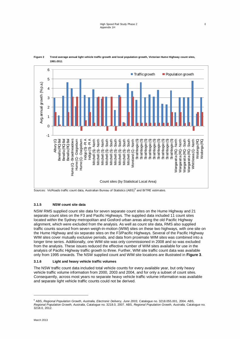
High Speed Rail Study Phase 2 Appendix 1H
March 2013
6
Figure 2 Trend average annual light vehicle traffic growth and local population growth, Victorian Hume Highway count sites, 1991-2011
Sources: VicRoads traffic count data, Australian Bureau of Statistics (ABS)5 and BITRE estimates.
3.1.5 NSW count site data
NSW RMS supplied count site data for seven separate count sites on the Hume Highway and 21 separate count sites on the F3 and Pacific Highways. The supplied data included 11 count sites located within the Sydney metropolitan and Gosford urban areas along the old Pacific Highway alignment, which were excluded from the analysis. As well as count site data, RMS also supplied traffic counts sourced from seven weigh-in-motion (WIM) sites on these two highways, with one site on the Hume Highway and six separate sites on the F3/Pacific Highways. Several of the Pacific Highway WIM sites cover mutually exclusive periods, and data from proximate WIM sites was combined into a longer time series. Additionally, one WIM site was only commissioned in 2008 and so was excluded from the analysis. These issues reduced the effective number of WIM sites available for use in the analysis of Pacific Highway traffic growth to three. Further, WIM site traffic count data was available only from 1995 onwards. The NSW supplied count and WIM site locations are illustrated in Figure 3.
3.1.6 Light and heavy vehicle traffic volumes
The NSW traffic count data included total vehicle counts for every available year, but only heavy vehicle traffic volume information from 2000, 2003 and 2004, and for only a subset of count sites. Consequently, across most years no separate heavy vehicle traffic volume information was available and separate light vehicle traffic counts could not be derived.
5 ABS, Regional Population Growth, Australia, Electronic Delivery, June 2003, Catalogue no. 3218.055.001, 2004. ABS, Regional Population Growth, Australia, Catalogue no. 3218.0, 2007. ABS, Regional Population Growth, Australia, Catalogue no. 3218.0, 2012.
-1
0
1
2
3
4
5
6
Albu
ry (C
)Be
nalla
(RC)
Bal
Bena
lla (R
C) B
alBe
nalla
(RC)
Bal
Hum
e (C
) -Br
oadm
eado
ws
Hum
e (C
) -Cr
aigi
ebur
nH
ume
(C) -
Crai
gieb
urn
Indi
go (S
) -Pt
AIn
digo
(S) -
Pt A
Mitc
hell
(S) -
Nor
thM
itche
ll (S
) -N
orth
Mitc
hell
(S) -
Nor
thM
itche
ll (S
) -So
uth
Mitc
hell
(S) -
Sout
hM
itche
ll (S
) -So
uth
Mitc
hell
(S) -
Sout
hM
itche
ll (S
) -So
uth
Mitc
hell
(S) -
Sout
hM
orel
and
(C) -
Nor
thSt
rath
bogi
e (S
)St
rath
bogi
e (S
)St
rath
bogi
e (S
)St
rath
bogi
e (S
)St
rath
bogi
e (S
)St
rath
bogi
e (S
)St
rath
bogi
e (S
)St
rath
bogi
e (S
)St
rath
bogi
e (S
)W
anga
ratt
a (R
C) -
Nor
thW
anga
ratt
a (R
C) -
Nor
thW
anga
ratt
a (R
C) -
Sout
hW
anga
ratt
a (R
C) -
Sout
hW
hitt
lese
a (C
) -N
orth
Wod
onga
(RC)
Wod
onga
(RC)
Avg.
annu
al g
row
th (%
p.a
.)
Count sites (by Statistical Local Area)
Traffic growth Population growth
Count sites (by Statistical Local Area)

High Speed Rail Study Phase 2 Appendix 1H
March 2013
7
WIM data includes counts of both light vehicles (Austroads Class 1 and 2 vehicles), which are detected but not weighed at each site, and heavy vehicles. While consideration was given to applying growth in heavy vehicle shares measured at WIM sites to regular count sites missing heavy vehicle count information, few of the count sites and WIM sites are located in sufficient close proximity to guarantee robust inferences about trends in heavy vehicle traffic volumes at those sites. In lieu of reliable heavy vehicle traffic volume data, heavy vehicle traffic shares were simply assumed to have remained more or less unchanged over the sample period and applied to missing years. For count sites located relatively close to Sydney or other major urban centres, heavy vehicle traffic shares are generally less than 15 per cent, so this assumption is unlikely to significantly affect implied light vehicle traffic growth. For other sites, where heavy vehicles can comprise between 30 and 40 per cent of total traffic, the inclusion of WIM data in the estimation of light vehicle traffic growth provides a measure of comparison. Figure 3 NSW traffic count site locations and weigh-in-motion
Source: RMS traffic count data.

High Speed Rail Study Phase 2 Appendix 1H
March 2013
8
3.1.7 Inter-capital and inter-regional light traffic volumes
Section 3.1.1 provided an outline of inter-capital light vehicle traffic volumes on the Hume Highway and is not repeated here. Comparison of traffic count data and NVS data implies that inter-capital travel is generally less than between 10 per cent of measured light vehicle traffic volumes on the Pacific Highway, with the share again varying by site location6. Consequently, local and shorter-distance inter-regional traffic are likely to account for the majority of measured growth in total light vehicle traffic volumes on this highway.
3.1.8 Traffic growth – NSW count sites
Averaged across all sites, total traffic grew by approximately 2.7 per cent a year between 1991 and 2011 on the Hume Highway in NSW. Light vehicle traffic grew by approximately two per cent per annum between 1991 and 2011 on the Hume Highway, with growth ranging from 1.4 per cent per annum at sites south of the Southern Highlands in NSW up to 3.2 per cent per annum on the outskirts of Sydney.
Averaged across all sites on the Pacific Highway, total traffic grew by approximately 4.6 per cent a year between 1991 and 2011. However, this appears to be inflated by measured traffic growth at three sites. Across other sites, traffic growth has varied between 1.6 and 4.5 per cent a year over this period.
Figure 4 shows the implied growth in light vehicle traffic volumes at NSW traffic count and WIM sites and local SLA population growth between 1991 and 2011. Similar to sites on the Hume Highway in Victoria, traffic growth has generally exceeded local population growth at most sites over that period. Figure 4 Trend average annual light vehicle traffic growth and local population growth, NSW Hume and Pacific Highway traffic count
sites, 1991–2011
Sources: State traffic count data, ABS (2004, 2007, 2012) and BITRE estimates.
6 BITRE (2006) estimates of inter-capital car traffic volumes for major inter-capital city pairs implies annual inter-capital car passenger numbers between Sydney-Brisbane, Sydney-Melbourne and the Gold Coast have generally been around 600,000 persons per annum between 1971 and 2010. Assuming an average vehicle occupancy of 2.5 persons per vehicle for inter-capital trips implies around 650 vehicles per day (both directions).
-0.5
1.5
3.5
5.5
7.5
9.5
11.5
Gre
ater
Hum
e Sh
ire (A
) Pt B
Yass
Val
ley (
A)
Gou
lbur
n M
ulw
aree
(A) B
al
Win
geca
rrib
ee (A
)
Win
geca
rrib
ee (A
)
Wol
lond
illy (
A)
Wol
lond
illy (
A)
Port
Ste
phen
s (A
)
Gos
ford
(C) -
Wes
t
Gos
ford
(C) -
Wes
t
Wyo
ng (A
) -N
orth
-Eas
t
Wyo
ng (A
) -N
orth
-Eas
t
Lake
Mac
quar
ie (C
) -N
orth
Lake
Mac
quar
ie (C
) -N
orth
Clar
ence
Val
ley (
A) -
Coas
t
Lake
Mac
quar
ie (C
) -N
orth
New
cast
le (C
) -O
uter
Wes
t
Sydn
ey
Twee
d (A
) -Pt
B /
Byro
n (A
)
Coff
s Har
bour
(C) -
Pt A
Has
tings
(A) /
Gre
ater
Tar
ee (C
)
Avg.
ann
ual g
row
th (%
p.a
.)
Count sites (by Statistical Local Area)
Traffic growth Population growth
Hume Hwy Pacific Hwy

High Speed Rail Study Phase 2 Appendix 1H
March 2013
9
3.2 Regional population SLA-level regional population data was sourced from ABS Regional Population Growth statistical releases in 2004, 2007 and 2012. Changes in statistical boundaries over that period were handled by first standardising all regional population estimates to the 2006 SLA boundaries, using ABS-supplied SLA-level population concordances, and then spatially matching regional areas to count sites.
Between census years, the regional population estimates are an approximation to the actual resident population, derived from the last census year population measurement and data and/or assumptions about fertility, mortality and regional migration patterns. This may affect the estimated travel elasticities. Figure 5 and Figure 6 show average annual population growth between 1991 and 2011, for NSW and Victorian SLAs. Figure 5 NSW average annual regional population growth, 1991–2011
Sources: ABS (2004, 2007, 2012) and BITRE estimates.

High Speed Rail Study Phase 2 Appendix 1H
March 2013
10
Figure 6 Victorian average annual regional population growth, 1991–2011
Sources: ABS (2004, 2007, 2012) and BITRE estimates.
3.3 Household income Consistent with the demand analysis in the HSR study, household income growth was proxied by growth in real GDP per capita7. BITRE also estimated the models using real gross national expenditure which measures real expenditure by Australian households. While real gross national expenditure grew approximately half a percentage point per year faster than real GDP between 1989 and 2011, and produces slightly different income elasticities, it did not improve the statistical performance of the models.
3.4 Travel costs/fuel prices Two alternative measures of travel cost were used in the empirical analysis: i) the private motoring price index, and ii) automotive fuel price index, both sourced from the Consumer Price Index collection and deflated by movements in the Consumer Price Index All Groups index8. While the choice of travel cost variable does affect the size and significance of the parameter estimate, the real automotive fuel price index has been used to align with wider assumptions in the HSR study.
3.5 Network changes Since 1991, there have been several major expansion and/or realignment projects along the Hume and Pacific Highways.
Construction of the Wangaratta (1994) and Albury-Wodonga (2007) bypasses have been main changes to the Hume Highway in Victoria over that time. Dummy variables were included in the analysis to account for the impact of these projects on the level of light vehicle traffic at nearby traffic count sites.
7 ABS, Australian System of National Accounts, 2010-11,Catalogue no. 5204.0, release date 28 October 2011. 8 ABS, Consumer Price Index Collection, 2012.

High Speed Rail Study Phase 2 Appendix 1H
March 2013
11
Along the Hume Highway in NSW, the main infrastructure upgrades since 1991 have been alignment changes, mainly the addition of the following town bypasses: Goulburn (1992), Yass (1994), Bookham (Northbound 1991, Southbound 1998) and Coolac (2007). Work is currently being completed to duplicate the remaining single carriageway sections in southern NSW and bypass Holbrook. With the exception of Goulburn and Yass, none of the count sites for which data was available are very close to these locations, and for Goulburn and Yass the available data does not overlap with the upgrade period, so these network changes were not explicitly accounted for in this analysis for this section of the corridor.
There have also been significant enhancements applied to the Pacific Highway over the sample period. These include duplication of highway sections at Bonville (9.6 kilometres, opened 2008), Brunswick Heads to Yelgun (8.6 kilometres, 2007), Nabiac (10 kilometres, 2006), Yelgun to Chinderah (14.5 kilometres, 2002) and bypass of Karuah (2004). Dummy variables were included in the models to account for the impact of these projects on the level of light vehicle traffic at count sites near the Yelgun-Chinderah section. No explicit adjustment was made for other upgrades sections as no count sites are located in close proximity to these sections.
4.0 Estimation specification and empirical analysis
4.1 Empirical specification BITRE modelled growth in traffic volumes across the available count sites using three separate empirical specifications, all based on the general formulation given in equation (1):
i. A simple ‘in-levels’ specification (equation 2).
ii. ‘Lagged-differences’ specification, around a base year T (equation 3).
iii. An error correction mechanism (ECM), which incorporates dynamic effects (equation 4).
log = log + log + + log + (2)
log log = log – log + log – log+ ( ) + (log log ) + (3)
log = log + log + + log +log log log log + (4)
Most variables are as defined in Section 2. The estimating specifications include separate population – P , denotes population in region I – and GDP per capita – Y denotes national per capita income – terms. The ECM specification includes short-run ( ) and long-run ( ) impacts (the in-levels specification is a restricted version of the ECM model). The parameter estimates were tested for statistical significance in order to derive the most parsimonious empirical specification. Separate ‘in-levels’ estimates were derived using both: 1) the raw traffic count data, which contained missing observations; and 2) ‘multiply-imputed’ traffic count data set, where missing traffic count observations were imputed using multiple imputation techniques (Rubin 1987, see discussion below)9. The ‘lagged differences’ specification was estimated using only the raw data and involved the use of different base years (T) across sites, due to differences in temporal data availability. Although the base year should be essentially arbitrary from the point of view of the analysis, it may have some effect on the results. The base year was chosen as close as possible to 2000–01 (the mid-point of the analysis period). The lagged differences specification effectively removes the site-specific constant terms from the regression. The ECM model estimates used the multiply-imputed data sets.
For each of the similar linear and ECM specifications, BITRE derived two sets of results: i) using a simple linear model with separate fixed effects for traffic volumes, and ii) including random effects to account for variation in the relationship between traffic growth and population/income across different 9 DB Rubin, Multiple Imputation for Nonresponse in Surveys, J Wiley and Sons, New York, 1987.

High Speed Rail Study Phase 2 Appendix 1H
March 2013
12
sites10. Owing to differences between jurisdictional data and potential differences in traffic growth across the Hume and Pacific Highways, separate estimates were made of traffic growth across each of the Hume Highway in Victoria, and the Hume Highway and the Pacific Highway in NSW. For all models, separate estimates were produced using unweighted data and weighting each observation by the number of recording/sampling days, to reflect the relative reliability of the measured count data. Weighting accords greater weight to observations based on a higher number of recording days, which should, in theory, exhibit less count variability. The Victorian data included the number of sampling days for all count sites. The NSW data, however, did not include the number of sampling days at non-WIM traffic count sites. Where this was the case, the number of sampling days was assumed equal to the total number of days in the year. The consequence of this assumption is that the days-weighted model results tend to be little different to the unweighted model results for NSW sections.
As already mentioned, all specifications included dummy variables to account for changes in network alignment over the period (for example, Wangaratta bypass c.1994 and Albury-Wodonga bypass 2007 at Victorian sites), and to also other account for other non-measurable effects such as unavailability of heavy vehicle counts at several sites between 1992 and 1994. These dummy variable parameter estimates are not reported in the estimation results. Models were also estimated using light vehicle traffic growth less BITRE-estimated inter-capital road-based trips11. However, as inter-capital passenger car trips typically represent less than 10 per cent of total road traffic volumes, removal of these trips did not significantly affect the estimation results.
4.2 Multiple imputation of missing data Multiple imputation methods were used to impute missing vehicle count and pre-1991 SLA-level populations, in order to estimate the ECM model specification which requires annual observations. For Victorian sites, missing vehicle count data comprised approximately 62 per cent of the annual number of records across all count sites and 58 per cent of total annual light vehicle counts across sites included in the analysis. Accordingly, BITRE generated 10 multiply-imputed data sets for the Victorian analysis.12 For NSW sites, the rate of missing vehicle count data was approximately 44 per cent on the Hume Highway and 42 per cent on the Pacific Highway, and again 10 imputations were generated. All imputations were generated using the Amelia II package13.
The impact of imputation was ‘tested’ by comparing the raw and multiply imputed data based ‘in-levels’ estimation results. In general, imputation had little impact on the sign and magnitude of the estimated parameters across Hume Highway sites, but did have a more significant impact on the Pacific Highway results. The multiply imputed data generally provided less variable and more sensible results than the raw data.
4.3 Estimation results 4.3.1 ‘In-levels’ specification results
Table 1 shows the ‘preferred’ specification model results for the raw data based ‘in-levels’ specification (equation 2). In all cases, the dependent variable is the natural logarithm of average daily light vehicle traffic volumes. The reported results include separate estimates based on the Hume Highway in Victoria, and the Hume Highway and the Pacific Highway in NSW, and separate estimates based on unweighted and recorded days-weighted estimation. The results reported were based on linear mixed effects (LME) specification, with site-specific fixed effects to account for variation in average traffic volumes across sites and site-specific random effects to account for site-specific variation in the relationship between traffic growth and the independent factors. All specifications are linear in logs, so the parameter estimates may be directly interpreted as (long-run) elasticities.
10 Use of the mixed effects specification allows for fixed variation in traffic levels across sites and random effects to capture average trend and variation in traffic growth from across the sample of available count sites. In other words, the count sites are treated as a sample of traffic growth across the road corridor of interest. 11 BITRE, op. cit. 12 The efficiency of estimates based on multiple imputations is 1 + where is the rate of missing information and m the number of imputations (Rubin op. cit.). For a missing information rate of between 50 and 70 per cent, the efficiency of 10 imputations is between 93 and 95 per cent and that of 20 imputations is between 97 and 98 per cent. 13 J Honaker, G King, M Blackwell, Amelia II: A Program for Missing Data, Journal of Statistical Software, 2011.

High Speed Rail Study Phase 2 Appendix 1H
March 2013
13
Table 1 ‘In-levels’ raw data based results
Hume Highway – Victoria Hume Highway – NSW Pacific Highway – NSW
Unweighted Days weighted Unweighted Days
weighted Unweighted Days weighted
Parameter estimates (fixed effects)
Local population 0.046 0.100 0.081 0.065 0.922 4.70
(0.095) (0.018) (0.150) (0.008) (0.385) (2.67)
GDP per capita 0.694 0.519 1.181 1.141 1.329 –0.889
(0.145) (0.023) (0.133) (0.007) (0.216) (0.169)
Fuel cost 0.002 –0.068 –0.367 –0.345 –0.087 –0.321
(0.089) (0.016) (0.067) (0.003) (0.083) (0.010)
Catchment population 1.161 1.446 NA NA NA NA
(0.215) (0.023)
Catchment distance 0.447 0.494 NA NA NA NA
Random effects (standard deviation)
Intercept 0.061 0.029 0.001 0.021 0.042 0.014
Local population 0.500 0.084 0.054 0.012 1.138 1.124
GDP per capita 0.383 0.100 0.008 0.002 0.047 0.710
Fuel cost 0.500 0.076 0.003 0.0002 0.15 0.041
Catchment population NE NE NE NE NE NE
Summary statistics
0.1040 0.05 0.002 0.042 0.082 0.034
R2 0.9862 0.9841 0.9984 0.9984 0.9956 0.9993
Log likelihood 282.7 –263.3 107.8 –125.3 126.8 –319.5 NA denotes not applicable. NE denotes not estimated. Note: Standard errors in parentheses. Intercept, site-specific constants and dummy variable parameter estimates not
shown. Source: BITRE estimates.
4.3.2 Victorian Hume Highway results
Columns 2 and 3 in Table 1 list the preferred raw model results for light vehicle traffic growth across Victorian traffic count sites between 1991 and 2011 (population data for 1989 and 1990 which was not readily available, so these years were excluded from the analysis). For both the weighted and unweighted results, the inclusion of the catchment population term is statistically significant, with the catchment population distance weighting approximately 0.5. The inclusion of catchment population reduces the magnitude of the local population term. The parameter estimates for local population, GDP per capita and fuel costs are all of the expected sign and nearly all are statistically significant. The mean per capita GDP elasticity is statistically significant and approximately 0.7 in the unweighted model, with a standard deviation across sites of approximately 0.4, and 0.5 in the days weighted specification, with a standard deviation across sites of 0.1. The fuel cost elasticity was generally negative and small (below -0.1) across most specifications and not statistically significant in the unweighted specification.

High Speed Rail Study Phase 2 Appendix 1H
March 2013
14
4.3.3 NSW Hume Highway results
Columns 4 and 5 in Table 1 list the preferred raw data based ‘in-levels’ model results for light vehicle traffic growth at NSW Hume Highway count sites. In contrast to the Victorian Hume Highway results, the catchment population term was not statistically significant across NSW Hume Highway sites. There is little difference between the unweighted and days weighted specifications. Information on the number of recording days was available for only a small number of NSW sites. The parameter estimates for local population, GDP per capita and real fuel costs are of the expected sign and generally statistically significant. Local population was not statistically significant in the unweighted specification. The results imply a GDP per capita elasticity of around 1.1 to 1.2, which is significantly higher than that derived for Victorian Hume Highway sites. The implied fuel cost elasticity is around –0.35 to –0.40, which implies travel is relatively inelastic to movements in fuel prices, but higher than the fuel price elasticity implied by the Victorian data.
4.3.4 NSW Pacific Highway results
Columns 6 and 7 in Table 1 list the preferred raw model results for light vehicle traffic growth across NSW Pacific Highway count sites. The estimation results exhibit significantly more variation across the different model specifications than for either of the two Hume Highway data sets. This variation disappears when the multiply-imputed data is used instead of the raw data, suggesting the small number of observations and variation affects the results. The equivalent results derived using the multiply-imputed data are listed in Sub appendix 1H.1, Table 4. The wider catchment-area population term was generally not statistically significant for data from this corridor. The parameter estimates for local population and fuel prices are of the expected signs, with rural traffic volumes being relatively inelastic with respect to fuel prices and local population having a more significant effect. The GDP per capita parameter estimate is of completely different signs depending on whether the estimates are weighted or not. The multiply-imputed parameter estimates, by contrast, are reasonably consistent and imply a GDP per capita elasticity of around 1.1 to 1.2 on the Pacific Highway (see Appendix 1H.1), Table 4.
4.3.5 ‘Lagged difference’ model results
Table 2 shows the ‘preferred’ estimation results for the lagged difference specification (equation 2). The lagged difference specification removes site-specific variation in traffic volumes. For estimation purposes, constant terms were included in the linear regressions in order to facilitate ready interpretability of the summary statistics, but they were generally not statistically significant. As for the in-levels model, several different specifications were estimated, including unweighted and days-weighted regressions and allowing for random parameter variation across sites. The lagged difference income elasticity estimates are generally similar in magnitude and sign to the in-levels estimates.

High Speed Rail Study Phase 2 Appendix 1H
March 2013
15
Table 2 ‘Lagged-differences’ raw data based results
Hume Highway – Victoria Hume Highway – NSW Pacific Highway – NSW
Unweighted Days weighted Unweighted Days
weighted Unweighted Days weighted
Parameter estimates (fixed effects)
Intercept –0.012 0.0004 –0.014 –0.028 –0.071 –0.061
(0.089) (0.028) (0.037) (0.012) (0.045) (0.039)
Local population –0.063 0.056 0.081 0.065 0.465 0.551
(0.086) (0.017) (0.150) (0.008) (0.104) (0.116)
GDP per capita 0.384 0.340 1.181 1.141 1.224 1.128
(0.153) (0.020) (0.133) (0.007) (0.161) (0.155)
Fuel cost 0.044 –0.038 –0.367 –0.345 0.074 0.053
(0.080) (0.006) (0.066) (0.003) (0.099) (0.091)
Catchment population 1.660 1.658 NA NA NA NA
(0.212) (0.020)
Catchment distance 0.911 0.847 NA NA NA NA
Random effects (standard deviation)
Intercept 0.056 0.025 0.022 0.013 NA NA
Local population 0.381 0.070 0.231 0.012 NA NA
GDP per capita 0.346 0.074 0.087 0.002 NA NA
Fuel cost 0.364 0.020 0.059 0.0001 NA NA
Catchment population NE NE NE NE NA NA
Summary statistics
0.092 0.041 0.023 0.041 0.118 1.965
R2 0.9528 0.9402 0.8934 0.8908 0.8770 0.8781
Log likelihood 256.3 –166.1 107.8 –125.3 141.7 153.9 NA denotes not applicable. NE denotes not estimated. Note: Standard errors in parentheses. Intercept, site-specific constants and dummy variable parameter estimates not
shown. Source: BITRE estimates.
Victorian Hume Highway results
Columns 2 and 3 of Table 2 show the lagged difference model results for light vehicle traffic growth for Victorian Hume Highway traffic count sites. The table includes unweighted and recording days weighted results. For both specifications, local population has little effect on traffic growth, but the catchment population parameter estimate, of approximately 1.6, is statistically greater than one. The optimal catchment distance is around 0.9, suggesting a surprisingly strong relationship between travel and regional population growth. The per capita GDP elasticity is around 0.35 to 0.40 implying that growth in travel on Victorian sections of the Hume Highway is relatively inelastic with respect to income. The estimates imply fuel cost has little effect on light travel on the Hume Highway in Victoria.

High Speed Rail Study Phase 2 Appendix 1H
March 2013
16
NSW Hume Highway results
Columns 4 and 5 of Table 2 show the preferred unweighted and days weighted lagged difference model results for light vehicle traffic growth across NSW Hume Highway traffic count sites. Preferred specifications include random variation in the parameter estimates. The catchment population parameter is not statistically significant across these sites. Again, there is little difference in the parameter values across the two specifications and the parameter estimates are broadly similar to the in-levels estimates in Table 1 (i.e. local population growth is marginally statistically significant, fuel prices have a statistically significant but relatively small impact on travel and the per capita income elasticity is quite significant and around 1.1 to 1.2).
NSW Pacific Highway results
Columns 6 and 7 of Table 2 show the preferred specification results for the lagged difference model of light vehicle traffic growth across NSW Pacific Highway traffic count sites between 1991 and 2011. The preferred specifications do not include site-specific random parameter variation. The catchment population term is not statistically significant across these sites. Again, like the results for NSW Hume Highway sites, there is little difference between the weighted and unweighted regression results. The estimates imply a local population elasticity of around 0.5 and per capita income elasticity of 1.1 to 1.2 for rural car travel on the Pacific Highway. The real fuel price parameter is not statistically significant, implying rural car travel on this section is relatively unresponsive to fuel prices.
4.3.6 ECM model results
Table 3 shows the model results for various multiply-imputed ECM model results (equation 3). In all cases, the dependent variable is the first difference of light vehicles traffic volumes. Again, the results report estimates for two separate specifications: i) unweighted and ii) days weighted, estimated separately using linear (LM) and LME specifications. All specifications are linear in logarithms, so the parameter estimates can be readily interpreted as elasticities. The ECM specification enables identification of short- and long-run impacts.
Victorian Hume Highway results
Columns 2–5 of Table 3 show the ECM model results for light vehicle traffic growth for Victorian Hume Highway traffic count sites between 1991 and 2011. The summary statistics imply that the LM specification results fit the data better than the LME specification, but there is generally little difference in the parameter estimates across the different specifications. The results shown in Table 3 are based on the unit distance weighted catchment population term (the distance weighting parameter was not estimated for the ECM specification, but the results for the non-distance weighted catchment population term are broadly similar). With the exception of local population, the first difference parameter terms are generally not statistically significant. The short-run local population term is statistically significant only in the LM specification, with an elasticity of around +0.1. The lagged dependent variable is strongly significant and around –0.8 to–0.9 across the different specifications, implying only a slight lag in dynamic response of travel to changes in income and fuel prices. The long-run local and catchment population terms are also statistically significant, and imply long-run elasticities of 0.25–0.36 and 0.6–1.1, respectively. The GDP per capita term implies a long-run elasticity of between 0.3 and 0.5. The inclusion of the catchment population term reduces the GDP per capita elasticity. Excluding the catchment population term, the long-run GDP per capita elasticity is around 0.8. The estimates imply fuel cost has little effect on rural light vehicle travel on the Hume Highway in Victoria.
NSW Hume Highway results
Columns 6–9 of Table 3 show the ECM model results for light vehicle traffic growth across NSW Hume Highway traffic count sites between 1991 and 2011. The summary statistics imply that the LME specification results fit the data slightly better than the LM specifications. The catchment population parameter is not statistically significant across these sites. With the exception of real fuel costs, the first difference variable parameter estimates are generally not statistically significant. The short-run real fuel cost term is statistically significant with an elasticity of around –0.27. The lagged dependent variable is strongly significant and around –1.0 across all specifications, implying a very short lag in rural travel response to changes in income and fuel prices. The GDP per capita term is strongly

High Speed Rail Study Phase 2 Appendix 1H
March 2013
17
significant, and implies a long-run income elasticity of around 1.1. The long-run fuel cost elasticity is around –0.4.
NSW Pacific Highway results
Columns 10–13 of Table 3 show the ECM model results for light vehicle traffic growth across NSW Pacific Highway traffic count sites between 1991 and 2011. Again, none of the first differences parameter estimates are statistically significant. The lagged dependent variable is strongly significant and around –0.9 in the LM estimates and –0.75 in the LME estimates, implying a short lag in long run rural travel response to changes in population, income and fuel prices. The lagged GDP per capita parameter estimate is strongly significant across all specifications, and implies a long-run income elasticity of around 1.5 to 1.6 across these sites (after allowing for lagged adjustment effects). The long-run local population and fuel cost elasticities are of the wrong sign, but generally not statistically significant.
4.4 Implications for long-term rural car travel growth The empirical results imply quite a degree of variation in population and income elasticity estimates across the three modelled road segments: i) the Hume Highway in Victoria, ii) Hume Highway in NSW, and iii) Pacific Highway in NSW. Fuel price responsiveness of rural car travel appears relatively consistent across the different road sections and model specifications, suggesting rural car travel is relatively insensitive to fuel prices. Within each road section, however, the parameter estimates derived for each model specification (i.e. in-levels, lagged differences and error correction model) are relatively consistent.

High Speed Rail Study Phase 2 Appendix 1H
March 2013
18
Table 3 Preferred multiply-imputed ECM model results
Hume Highway – Victoria Hume Highway – NSW Pacific Highway – NSW
Unweighed Days weighted Unweighed Days weighted Unweighed Days weighted
LM LME LM LME LM LME LM LME LM LME LM LME
Parameter estimates (fixed effects)
First differences
Local population 0.145 0.061 0.113 0.085 –0.097 –0.625 –0.045 –0.474 0.343 0.349 0.338 0.681
(0.047) (0.067) (0.041) (0.064) (1.434) (1.709) (1.457) (0.796) (0.268) (0.272) (0.266) (1.188)
GDP per capita 0.413 –0.393 –0.813 –0.721 0.338 0.293 0.324 0.296 0.874 0.330 1.020 0.465
(0.713) (0.510) (0.559) (0.633) (1.181) (1.215) (1.144) (0.863) (1.427) (1.995) (1.236) (0.904)
Fuel cost –0.085 –0.024 0.077 0.030 –0.274 –0.273 –0.266 –0.267 0.094 0.092 0.057 0.070
(0.063) (0.081) (0.104) (0.113) (0.127) (0.131) (0.134) (0.092) (0.175) (0.182) (0.157) (0.095)
Catchment population –1.764 –0.736 –0.208 0.587 NA NA NA NA NA NA NA NA
(4.535) (3.781) (0.582) (0.457)
Catchment distance 1 1 1 1 NA NA NA NA NA NA NA NA
Lagged variables
LV AADT –0.887 –0.768 –0.894 –0.761 –1.064 –1.084 –1.066 –1.080 –0.897 –0.743 –0.933 –0.733
(0.059) (0.054) (0.050) (0.055) (0.127) (0.153) (0.152) (0.135) (0.124) (0.100) (0.113) (0.068)
Local population 0.324 0.276 0.228 0.228 0.145 0.137 0.118 0.112 –0.296 –0.370 –0.268 –0.374
(0.051) (0.036) (0.043) (0.040) (0.241) (0.236) (0.240) (0.139) (0.180) (0.191) (0.188) (0.096)
GDP per capita 0.277 0.319 0.309 0.404 1.113 1.141 1.140 1.160 1.371 1.186 1.462 1.221
(0.261) (0.174) (0.218) (0.177) (0.299) (0.313) (0.293) (0.217) (0.296) (0.278) (0.289) (0.177)

High Speed Rail Study Phase 2 Appendix 1H
March 2013
19
Table 3 (continued)
Hume Highway – Victoria Hume Highway – NSW Pacific Highway – NSW
Unweighed Days weighted Unweighed Days weighted Unweighed Days weighted
LM LME LM LME LM LME LM LME LM LME LM LME
Fuel cost –0.012 0.003 0.057 0.038 –0.407 –0.411 –0.409 –0.411 0.238 0.239 0.143 0.165
(0.100) (0.097) (0.098) (0.103) (0.157) (0.161) (0.160) (0.117) (0.192) (0.194) (0.174) (0.091)
Catchment population 1.001 0.685 0.898 0.446 NA NA NA NA NA NA NA NA
(0.299) (0.213) (0.381) (0.293)
Random effects (standard deviation)
Intercept NA 0.045 NA 0.027 NA 0.031 NA 0.013 NA 0.064 NA 4.15e–07
Population NA 0.025 NA 0.106 NA 1.943 NA 0.082 NA 0.008 NA 0.121
GDP per capita NA 0.487 NA 1.682 NA 0.753 NA 0.030 NA 4.755 NA 0.177
Fuel cost NA 0.039 NA 0.071 NA 0.065 NA 0.004 NA 0.222 NA 0.007
Catchment population NA NE NA NE NA NE NA NE NA NE NA NE
Summary statistics
0.5971 0.1380 0.1690 0.1772 0.090 0.087 1.662 0.087 0.197 0.197 3.150 0.181
R2 0.4489 0.3680 0.4202 0.3857 0.5738 0.6051 0.5785 0.5983 0.3681 0.3886 0.4033 0.3701
Log likelihood 347.69 –1573.9 425.56 358.21 147.41 119.25 145.95 –289.51 73.61 21.87 102.29 –804.59 NA denotes not applicable. NE denotes not estimated. Note: Standard errors in parentheses. Intercept, site-specific constants and dummy variable parameter estimates not shown. Source: BITRE estimates.

High Speed Rail Study Phase 2 Appendix 1H
March 2013
20
On Victorian Hume Highway sections, the (long-run) income elasticity is statistically significant, generally ranging between 0.4 and 0.7, depending on the empirical specification and variables included. If the distance-weighted catchment population term is excluded, the income elasticity on Victorian Hume Highway sections was around 0.8 to 1.0. Across all model specifications, however, the empirical results imply an income elasticity statistically significantly less than one. By contrast, the model estimates for count sites on the Hume and Pacific Highways in NSW imply a higher (long-run) income elasticity for rural car travel, typically around 1.1 to 1.2. The distance-weighted catchment population term was generally not statistically significant across these highway sections. Factors that might account for some of the estimated difference in the income elasticity of rural car travel across these different sections could include inherent differences in the mix and type of rural car trips, relative distribution of count sites and input data accuracy.
Travel mix and behaviour
Part of the difference in estimated income elasticities across different highway sections could be due to inherent differences in the type and mix of trips on the two highways. It may be that the mix of rural car trips on the Hume Highway in Victoria entail a greater share of shorter-distance, less discretionary trips than either of the Hume or Pacific Highways in NSW. However, as stated at the outset, there is little information available on the relative mix of rural car trip types and lengths.
Count site location impacts
Differences in the relative geographic distribution of available traffic count site data across the three different highway segments may contribute to some of the difference in the estimated income elasticity, particularly between NSW and Victorian sections of the Hume Highway. The Victorian data provides a more evenly distributed set of counts across the length of the highway, whereas the NSW count sites, both on the Hume and Pacific Highways, are predominantly located closer to Sydney. The more even geographic distribution may mean that the Victorian data includes more observations at sites where shorter-distance farm to local rural town trips are a greater proportion of the traffic stream, and hence affect the measured income and price elasticities. Again, with relatively little available information on the composition of car travel across different sites, it is not possible to determine how significant this effect is.
Population and household income measures
As noted in Section 3, between census years, regional population data is an approximation to the actual resident population, based on data and/or assumptions about trends in births, deaths and regional migration patterns. Intercensal disparity in regional population estimates may also explain some of the relative difference in estimated elasticities across the different corridors. In a similar vein, per capita GDP is a very blunt approximation to changes in household incomes, which may vary considerably across urban and rural regional areas. Were household income growth is available at a regional level, it might account for some of the estimated variation in the income elasticity across the different corridors.
Choice of long-run income elasticity
In considering the long-run income elasticity to apply to future rural car travel across the corridor, the separate Victorian and NSW section results present a choice between an income elasticity either slightly below one or slightly above one. For forecasting potential future rural car travel in the HSR corridor, a long-run income elasticity of 0.8 has been chosen for long-distance car trips, and about half that for shorter-distance rural car trips. Influential in opting for these values is the judged relative robustness of the Victorian-based estimation results, e.g. greater number of count sites, generally more observations per site and more evenly distributed geographic coverage of sites. These elasticity values also imply more conservative estimates of likely future rural car travel demand, which is generally consistent with the approach adopted across the HSR study.

High Speed Rail Study Phase 2 Appendix 1H
March 2013
21
5.0 Concluding remarks This paper has outlined the methods and empirical results of analysis of the relationship between historical growth in light vehicle traffic on the Hume and Pacific Highways and growth in regional populations, per capita GDP, a proxy for household income growth, and real fuel prices. The primary purpose of the analysis was to determine the significance and size of the relationship between household income growth and rural light vehicle traffic volumes. The analysis estimated separate relationships for each of: i) the Hume Highway in Victoria; ii) the Hume Highway in NSW and iii) the Pacific Highway in NSW, using a range of different empirical specifications.
The empirical results imply a statistically significant and positive relationship between rural light vehicle traffic growth and per capita GDP across the corridor. The Victorian Hume Highway data implies an average income elasticity for light vehicle rural traffic volumes of around 0.5 to 0.8, depending on the estimation method, and the NSW Hume and Pacific Highway data implies an average income elasticity of around 1.1 to 1.2. The results also imply local and regional population growth has a small but positive effect on rural traffic volumes, but that rural travel is relatively insensitive to changes in fuel prices. For forecasting potential future rural car travel in the HSR corridor, a long-run elasticity of 0.8 would appear to be appropriate for long-distance rural travel, and a lower elasticity value for shorter-distance rural trips.

High Speed Rail Study Phase 2 Appendix 1H
March 2013
22
Sub appendix 1H.1 Additional empirical results Table 4 Multiply-imputed ‘in-levels’ preferred specification estimates
Hume Highway – Victoria Hume Highway – NSW Pacific Highway – NSW
Unweighed Days weighted Unweighed Days
weighted Unweighed Days weighted
Parameter estimates (fixed effects)
Local population 0.209 0.252 0.125 0.114 0.549 0.573
(0.077) (0.072) (0.231) (0.116) (0.450) (0.169)
GDP per capita 0.982 0.965 0.990 0.991 1.216 1.159
(0.124) (0.113) (0.246) (0.143) (0.326) (0.148)
Fuel cost 0.132 0.081 –0.289 –0.279 0.113 0.107
(0.093) (0.091) (0.122) (0.089) (0.143) (0.075)
Catchment population NA NA NA NA NA NA
Catchment distance NA NA NA NA NA NA
Random effects (standard deviation)
Intercept 0.032 0.027 0.041 0.031 0.050 0.049
Local population 0.220 0.046 0.089 0.007 0.829 0.039
GDP per capita 0.262 0.045 0.189 0.011 0.460 0.021
Fuel cost 0.155 0.042 0.087 0.005 0.322 0.018
Catchment population NE NE NE NE NE NE
Summary statistics
0.150 0.120 0.090 0.090 0.129 0.126
R2 0.9325 0.9294 0.9919 0.9919 0.9860 0.9856
Log likelihood 506.06 –1229.2 122.37 –309.67 135.59 –755.45 NA denotes not applicable. NE denotes not estimated. Note: Standard errors in parentheses. Intercept, site-specific constants and dummy variable parameter estimates not
shown. Source: BITRE estimates.


Related Documents


![Zorgbehoeftenonderzoek [BOOZ]t](https://static.cupdf.com/doc/110x72/557807f9d8b42aa5488b4e2b/zorgbehoeftenonderzoek-boozt.jpg)


