High-resolution tropospheric ozone fields for INTEX and ARCTAS from IONS ozonesondes

High‐resolution tropospheric ozone fields for INTEXand ARCTAS from IONS ozonesondes

D. W. Tarasick,1 J. J. Jin,2,3 V. E. Fioletov,1 G. Liu,1,4 A. M. Thompson,5 S. J. Oltmans,6

J. Liu,1 C. E. Sioris,1 X. Liu,7,8 O. R. Cooper,9,10 T. Dann,11 and V. Thouret12

Received 29 July 2009; revised 11 May 2010; accepted 17 May 2010; published 19 October 2010.

[1] The IONS‐04, IONS‐06, and ARC‐IONS ozone sounding campaigns over NorthAmerica in 2004, 2006, and 2008 obtained approximately 1400 profiles, in five series ofcoordinated and closely spaced (typically daily) launches. Although this coverage isunprecedented, it is still somewhat sparse in its geographical spacing. Here we use forwardand back trajectory calculations for each sounding to map ozone measurements to anumber of other locations and so to fill in the spatial domain. This is possible because thelifetime of ozone in the troposphere is of the order of weeks. The trajectory‐mapped ozonevalues show reasonable agreement, where they overlap, to the actual soundings, andthe patterns produced separately by forward and backward trajectory calculations aresimilar. Comparisons with MOZAIC profiles and surface station data show generally goodagreement. A variable‐length smoothing algorithm is used to fill data gaps: for each pointon the map, the smoothing radius is such that a minimum of 10 data points are included inthe average. The total tropospheric ozone column maps calculated by integrating thesmoothed fields agree well with similar maps derived from TOMS and OMI/MLSmeasurements. The resulting three‐dimensional picture of the tropospheric ozone field forthe INTEX and ARCTAS periods facilitates visualization and comparison of differentyears and seasons and will be useful to other researchers.

Citation: Tarasick, D. W., et al. (2010), High‐resolution tropospheric ozone fields for INTEX and ARCTAS from IONSozonesondes, J. Geophys. Res., 115, D20301, doi:10.1029/2009JD012918.

1. Introduction

[2] Ozone plays a major role in the chemical and radiativebalance of the troposphere. It controls the oxidizing capacity

of the lower atmosphere (it is a primary precursor to theformation of OH radicals) and thereby the capacity of thelower atmosphere to remove other pollutants. Ozone acts asan important infrared absorber (greenhouse gas), particularlyin the upper troposphere, and, because of multiple scatter-ing, is more effective in filtering UV‐B than its smallabundance in the troposphere (about 10% of the total col-umn) would suggest. However, at ground level, ozone isresponsible for significant damage to forests and crops andis a principal factor in air quality, as it has adverse effects onhuman respiratory health [Jerrett et al., 2009].[3] Ozone soundings are the major source of information

on ozone amounts in the free troposphere. When properlyprepared and handled, electrochemical concentration cell(ECC) ozonesondes have a precision of 3%–5% and anabsolute accuracy of about 10% in the troposphere [Smit et al.,2007; Kerr et al., 1994; Deshler et al., 2008; Liu et al.,2009]. The ozone sensor response time (e−1) of about 25 sgives the sonde a vertical resolution of about 100 m for atypical balloon ascent rate of 4 m/s in the troposphere. Twotypes of ECC ozonesondes are in current use, the 2Z modelmanufactured by EnSci Corp. and the 6A model manufac-tured by Science Pump, with minor differences in con-struction and some variation in recommended concentrationsof the potassium iodide sensing solution and of its phosphatebuffer. The maximum variation in tropospheric response

1Air Quality Research Division, Environment Canada, Downsview,Ontario, Canada.

2Department of Earth and Space Science and Engineering, YorkUniversity, Toronto, Ontario, Canada.

3Now at Jet Propulsion Laboratory, California Institute of Technology,Pasadena, California, USA.

4Now at Space Sciences Laboratory, University of California, Berkeley,California, USA.

5Department of Meteorology, Pennsylvania State University,University Park, Pennsylvania, USA.

6NOAA Climate Monitoring and Diagnostics Laboratory, Boulder,Colorado, USA.

7Goddard Earth Sciences and Technology Center, University ofMaryland, Baltimore, Maryland, USA.

8Harvard‐Smithsonian Center for Astrophysics, Cambridge,Massachusetts, USA.

9Cooperative Institute for Research in Environmental Sciences,University of Colorado, Boulder, Colorado, USA.

10NOAA Earth System Research Laboratory, Boulder, Colorado, USA.11Air Quality Research Division, Environment Canada, Ottawa,

Ontario, Canada.12Laboratoire d’Aerologie, Centre National de la Recherche

Scientifique, Observatoire Midi‐Pyrenees, Toulouse, France.

Published in 2010 by the American Geophysical Union.

JOURNAL OF GEOPHYSICAL RESEARCH, VOL. 115, D20301, doi:10.1029/2009JD012918, 2010

D20301 1 of 12

resulting from these differences is likely on the order of2%–3% [Smit et al., 2007].[4] Although the vertical resolution of ozone soundings is

excellent, their geographical and temporal coverage issparse. Worldwide, there are currently about 60 ozonesondestations making regular soundings and reporting the datato the World Ozone and Ultraviolet Radiation Data Center(WOUDC; http://www.woudc.org/). Most make weeklysoundings. However, during the ICARTT (InternationalConsortium for Atmospheric Research on Transport andTransformation) INTEX (Intercontinental Chemical Trans-port Experiment) field campaigns (1 July to 15 August 2004),Environment Canada (EC), the National Aeronautics andSpace Administration (NASA), the National Oceanic andAtmospheric Administration (NOAA), and several U. S. uni-versities pooled resources to release 275 ozonesondes from adozen sites across the eastern United States and Canada underthe IONS‐04 (INTEX Ozonesonde Network Study 2004)program [Thompson et al., 2007a, 2007b]. This representedthe largest single set of free tropospheric ozone measure-ments ever compiled (as of 2004) for this region.[5] A second IONS campaign, IONS‐06, was carried out

in 2006, to complement the INTEX‐B and TEXAQS aircraftand model studies. This campaign provided more completecoverage of North America, with more sites and launches: atotal of 740 sonde profiles were taken from 23 sites.[6] In 2008, the ARC‐IONS (ARCTAS Intensive Ozo-

nesonde Network Study) campaign was undertaken incooperation with the NASA project Arctic Research of theComposition of the Troposphere from Aircraft and Satellites(ARCTAS), with sites in Canada, Alaska, Greenland, andthe northern United States. It consisted of two phases (Apriland July) with 17 sites, most launching daily, for a total ofmore than 380 profiles.[7] The IONS coordinated intensive observational cam-

paigns have provided a unique set of ozone profile mea-surements over North America. The data have been usedextensively to study tropospheric ozone processes and theircontribution to the ozone budget [e.g., Cooper et al., 2006,2007; Thompson et al., 2007a, 2007b, 2008; Tarasick et al.,

2007; Pfister et al., 2008; Yorks et al., 2009] for validationof satellite measurements [Parrington et al., 2008, 2009;Stajner et al., 2008; Schoeberl et al., 2007; Nassar et al.,2008; Jiang et al., 2007; Dupuy et al., 2009; Livingstonet al., 2007; Nardi et al., 2008] and for initialization andvalidation of models [Chai et al., 2007; Pierce et al., 2007,2009; Yu et al., 2007; Tang et al., 2008].[8] Although the geographical and temporal coverage of

the IONS measurements is more than 5 times greater thanthat of regular network launches, it is still somewhat sparsein its geographical spacing. However, as the lifetime ofozone in the troposphere is of the order of weeks, a mea-surement of ozone mixing ratio at one place and time alsoprovides an good estimate of ozone mixing ratio in thatsame air parcel several hours or days before and after. It istherefore possible to employ a technique that has beenused successfully in the stratosphere [Sutton et al., 1994;Newman and Schoeberl, 1995; Morris et al., 2000] and useforward and back trajectory calculations for each soundingto map ozone measurements to a number of other locationsand so to fill in the spatial domain. In the troposphere, tra-jectories have larger errors than in the stratosphere [Stohland Seibert, 1997], primarily because of the importance ofvertical motion, which is difficult to compute accurately,but also because of turbulence in the boundary layer.Nevertheless, trajectory‐based domain‐filling models havebeen used successfully to extend ozone climatologies basedon MOZAIC aircraft data [Stohl et al., 2001], to recon-struct tropospheric water vapor fields [Pierrehumbert, 1998;Pierrehumbert and Roca, 1998; Dessler and Minschwaner,2007], and to analyze small‐scale variations in ozonemixing ratio observed by research aircraft [Methven et al.,2003].

2. Data and Method

2.1. Ozonesonde Profiles

[9] During the three IONS campaigns ozonesonde profile,data were collected at the sites described in Tables 1–3. Atall sites electrochemical concentration cell (ECC) ozone-sondes were used, either the 2Z model manufactured byEnSci Corp. or the 6Amodel manufactured by Science Pump,with some variation in concentration of the KI sensing solu-tion and of its phosphate buffer. Sounding frequency varied,from as often as twice daily to as little as weekly, as may beseen from the column indicating the number of availableprofiles for each site. Sonde release times also varied betweensites but were generally constant, within a campaign, for eachsite. In general sonde releases were timed to coincide withsatellite overpasses and with the maximum in the diurnalcycle of tropospheric ozone (∼1–3 p.m. local standardtime), except where prescribed by operational weatherservice requirements (as for many of the Canadian sites,which launch at 11 or 23 UT).

2.2. Data Mapping

[10] Ozone profile data were first converted to 1 kmaltitude resolution. Ozone partial pressures were averagedfor 1 km layers starting at sea level, where altitude wascalculated from the measured temperature profile using thehydrostatic relation. These were then divided by the average

Table 1. IONS‐04 Sites for the July 1 to 15 August 2004 StudyPeriod

Sounding Site

Location

No. ofProfiles

ReleaseTime

Lat(°N)

Long(°W)

Alt(m) UT LST

CanadaEgbert, ON 44.23 79.78 251 5 11 6Sable Is., NS 43.93 60.01 4 33 23 18Yarmouth, NS 43.87 66.12 9 15 17 12

USARon Brown research vessel,

Gulf of Maine ∼43.3 ∼69.5 0 33 15 10Beltsville, MD 39.04 76.52 24 8 14 9Boulder, CO 40.30 105.20 1743 7 17 10Houston, TX 29.87 95.33 19 25 19 13Huntsville, AL 34.73 86.58 196 14 19 13Narragansett, RI 41.52 71.32 21 39 18 13Pellston, MI 45.57 84.68 235 38 18 13Trinidad Head, CA 41.05 124.15 20 20 18 10Wallops Is., VA 37.85 75.50 13 18 17 12

TARASICK ET AL.: TROPOSPHERIC OZONE FIELDS FROM IONS D20301D20301

2 of 12

pressure in the layer to produce values for average ozonemixing ratio. The tropopause height was calculated for eachprofile according to the World Meteorological Organization[1992] criterion, that is, the lowest height at which thetemperature lapse rate falls to 2°C/km or less, provided thatthe average lapse rate for 2 km above this height is also notmore than 2°C/km. The layer containing the tropopause andthose above were not used.[11] For each location, at 1 km height intervals (0.5 km,

1.5 km, etc.) forward and back trajectories were calculatedusing version 4.8 of the HYSPLIT model [Draxler and Hess,1997, 1998], developed by the NOAA Air Resources Labo-ratory (NOAA ARL). The meteorological input for the tra-jectory model was the global NOAA‐NCEP/NCAR (NationalCenters for Environmental Prediction/National Center forAtmospheric Research) pressure level reanalysis data set.Each trajectory was calculated for 96 h duration, and theoriginal data were mapped to the locations calculated forevery 6 h along the forward and back trajectories. In this way,each original measurement was mapped into 32 additionalozone mixing ratio values.[12] As a quality check, maps produced using only for-

ward trajectories or only back trajectories were compared.These showed, in a few cases, anomalous differences thatcould be traced to measurements near particularly strongozone sources. At such points, rapid local ozone productioncan overwhelm the contribution from advection. The localmeasurement is therefore not representative of past his-tory, and the back trajectory mapping of the measured ozoneis invalid. Such back trajectories were removed. (The for-ward trajectory‐mapped values were presumed still valid.)Although all five IONS campaigns and all levels weresimilarly examined, only a small number of back trajectories

needed to be removed, primarily from the Houston area,Mexico City, and Holtville, CA, in the summers of 2004and 2006.[13] The original and trajectory‐mapped data were then

averaged into bins measuring 1° latitude by 1° longitude,at each 1 km altitude, for the duration of each campaign(∼1 month in each case). Two different altitude coordinateswere employed for this binning, and so two sets of maps

Table 2. IONS‐06 Sites for the March to May (INTEX‐B) and August 2006 Study Periods

Sounding Site

Location No. of Profiles Release Time

Lat (°N) Long (°W) Alt (m) March April–May August UT LST

CanadaBratt’s Lake, SK 50.20 104.70 580 2 30 29 21 15Edmonton, AB 53.55 114.11 766 3 4 4 11 4Egbert, ON 44.23 79.78 251 3 5 15 19 14Kelowna, BC 49.93 119.40 456 2 26 27 23 15Sable Is., NS 43.93 60.01 4 28 23 18Walsingham, ON 42.64 80.60 200 21 20 1,13 20,8Yarmouth, NS 43.87 66.12 9 3 5 13 23 18

USARon Brown research vessel, Gulf of Mexico ∼29.0 ∼95.0 0 38 18 12Barbados 13.20 59.50 0 27 17 13Beltsville, MD 39.04 76.52 24 12 18 13Boulder, CO 40.30 105.20 1743 4 5 34 19 12Holtville, CA 32.80 115.40 −19 20 20 12Houston, TX 29.72 95.40 19 17 7 19 20 14Huntsville, AL 35.28 86.58 196 11 3 33 18 12Narragansett, RI 41.52 71.32 21 2 13 30 17 12Paradox, NY 43.92 73.64 284 5 19 14Socorro, NM 34.6 106.9 1402 27 19 12Table Mountain, CA 34.40 117.70 2285 3 2 31 20 12Trinidad Head, CA 41.05 124.15 20 6 15 31 20 12Valparaiso, IN 41.50 87.00 240 15 5 19 14Wallops Is., VA 37.87 75.50 13 5 7 11 17 12Richland, WA 46.20 119.16 123 24 21 13

MexicoMexico City 19.42 98.58 2272 14 21 18 12

Table 3. ARC‐IONS Sites for the April and July 2008 StudyPeriods

Sounding Site

LocationNo. ofProfiles

ReleaseTime

Lat(°N)

Long(°W)

Alt(m) April July UT LST

CanadaBratt’s Lake, SK 50.20 104.70 580 15 14 21 15Churchill, MB 58.74 94.07 30 17 10 23 17Edmonton, AB 53.55 114.11 766 19 16 23 16Egbert, ON 44.23 79.78 251 11 18 13Eureka, NU 79.99 85.94 10 19 1 23 18Goose Bay, NL 53.32 60.30 44 15 23 19Kelowna, BC 49.93 119.40 456 13 14 23 15Resolute, NU 74.71 94.97 46 17 2 23 17Sable Is., NS 43.93 60.01 4 12 15 23 18Whitehorse, YT 60.70 135.07 704 12 15 23 15Yarmouth, NS 43.87 66.12 9 15 23 18Yellowknife, NT 62.50 114.48 210 19 19 12

USABarrow, AK 71.32 156.60 11 20 21 12Boulder, CO 40.30 105.20 1743 13 19 12Narragansett, RI 41.52 71.32 21 4 3 16 11Summit, Greenland 72.57 38.48 3238 19 18 14 11Trinidad Head, CA 41.05 124.15 20 18 17 19 11

TARASICK ET AL.: TROPOSPHERIC OZONE FIELDS FROM IONS D20301D20301

3 of 12

were produced: one binned by altitude above sea level andthe other binned by altitude above ground level.[14] Both sets of maps are presented with and without

smoothing. For the smoothed maps, a variable‐lengthsmoothing algorithm is employed: each 1 × 1° pixel on themap is replaced by the simple average of all data pointswithin a radius of 1°–10°, the smoothing radius beingmade just large enough that a minimum of 10 data pointsare included in each average. The parameters of 10° radius(1–2 correlation lengths for ozone in the troposphere) and10 points are evidently somewhat arbitrary and weredetermined empirically. Where the data density is high,these parameters imply that for some pixels no smoothing isapplied. No average is calculated for locations that do nothave 10 data points within a 10° radius.

2.3. Accuracy

[15] The accuracy of these results depends upon theaccuracy of the calculated trajectories and also on theassumption that ozone chemistry can be neglected over a4‐day time scale. The latter assumption is generally valid,

since the average lifetime of ozone is about 22 days in thetroposphere [Stevenson et al., 2006], although it varies withlatitude, altitude, and season [von Kuhlmann et al., 2003;Roelofs and Lelieveld, 1997]. However, as is well known,in pollution plumes photochemistry can produce ozone ontime scales of a few days [e.g., Mao et al., 2006], so thisassumption can be violated in certain circumstances, asdescribed below.[16] A number of studies have attempted to estimate the

accuracy of trajectories by several different methods.Downey et al. [1990] estimate typical errors of 350 km for4 day trajectories based on estimated wind errors. Stohl[1998] gives a comprehensive review of studies usingballoons, material tracers, smoke plumes, and Saharan dustto evaluate trajectory errors and quotes typical errors of 20%of the trajectory distance or about 100–200 km/d (with widevariation between studies). More recently, Harris et al.[2005] evaluate trajectory model sensitivity to uncertaintiesin input meteorological fields and find uncertainties of30%–40% of the horizontal trajectory distance or 600–1000 km after 4 days, while Engström and Magnusson[2009], using an ensemble analysis method, find typicalerrors in the northern hemisphere of 350–400 km after3 days and ∼600 km after 4 days.

x

xxx

x

x

x

xx

x

x x

x

x

x

x

xx

xx

x

x

Figure 1. (top) Trajectory‐mapped ozone field at 2–3 kmabove ground level, from the IONS soundings for August2006. The original data set is 480 soundings from 22 sites.The individual (1° × 1°) pixel averages are shown. Thelocations of the sounding sites contributing data to this mapare also indicated. (bottom) Smoothed version of the ozonefield in the upper figure (see text).

Figure 2. (top) The number of data points contributing tothe averages in Figure 1. (bottom) The standard error inppb for each (1° × 1°) pixel average.

TARASICK ET AL.: TROPOSPHERIC OZONE FIELDS FROM IONS D20301D20301

4 of 12

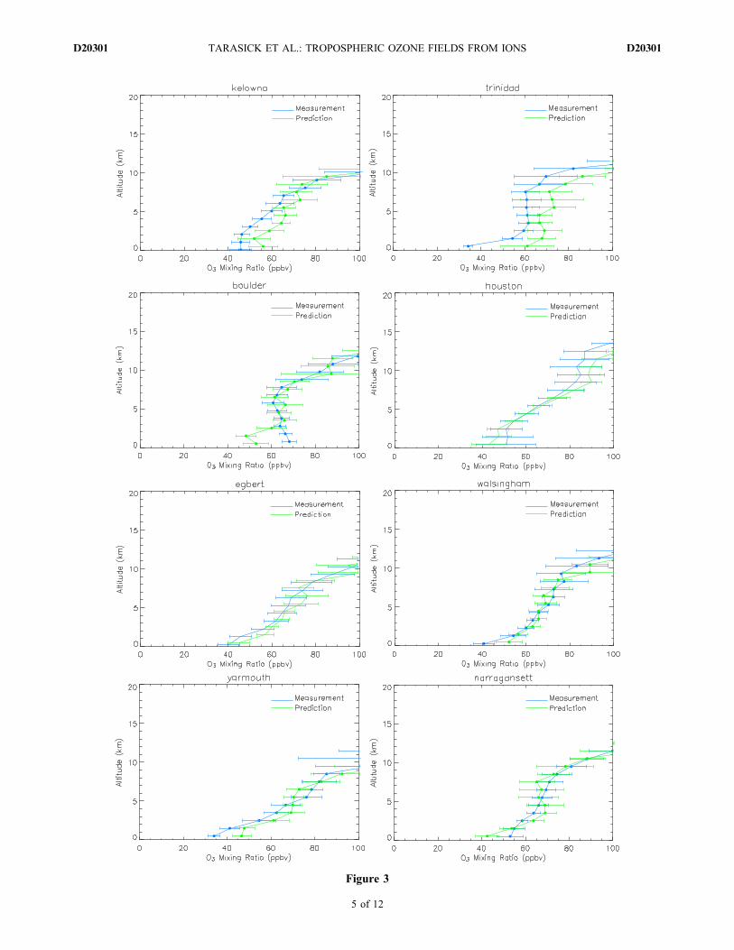
Figure 3

TARASICK ET AL.: TROPOSPHERIC OZONE FIELDS FROM IONS D20301D20301

5 of 12

[17] Calculated correlations between ozone values overNorth America from Aura OMI (Ozone MonitoringInstrument) retrievals [Liu et al., 2005, 2009a, 2009b], andtrajectory‐mapped ozone soundings at different altitudes(not shown) decrease with time for 1, 2, 3, and 4 days’ lag,indicating a decline in accuracy with time (or trajectorylength) of the trajectory‐mapped ozone values that is con-sistent with the discussion above; that is, trajectory errorincreases with time. Correlations are also in general non‐negligible even at 4 days’ lag. Since this lag is considerablylonger, both in time and average trajectory length, thantypical correlation time scales (or distances) for ozone in thetroposphere [Liu et al., 2009], it implies (as expected basedon the discussion above) that the trajectory‐mapped valueshave useful information even after 4 days.[18] The estimates of ∼100–200 km/d quoted above rep-

resent errors for individual trajectories in the troposphere.Errors in the final product should be much reduced byaveraging of multiple trajectories. However, in the planetaryboundary layer (PBL), complex dispersion and turbulencetends to render single trajectories less representative of theactual flow [Stohl and Seibert, 1997], and several authorssuggest using an ensemble of trajectories [Merrill et al.,1985; Stohl, 1998]. In the PBL therefore the averaging ofozone values from multiple trajectories in each pixel, as

well as subsequent horizontal averaging (smoothing), willbe particularly important for reducing trajectory errors.Nevertheless, we expect results for the lowest (0–1 km)layer to be less accurate than for higher levels.

3. Results and Discussion

3.1. Validation

[19] Figure 1 (top) shows an example of a trajectory‐mapped ozone field produced by the procedure describedabove. The original data set of approximately 480 mea-surements has been mapped into some 15,800 data values(not precisely 33 × 480, as air parcels do not necessarilyremain within an altitude level for the entire 96 h durationof a trajectory). Coverage of North America is quite good,and although there appears to be considerable variationbetween nearby pixels in some cases, the map shows fea-tures expected of the ozone distribution at this altitude: highvalues near Mexico City and over the Atlantic Ocean off theeastern seaboard, and low values over northern Canada andvery low values over the Caribbean. Higher values over theRocky Mountains reflect the fact that this map is for 2–3 kmabove ground level, which is the middle troposphere abovethe Rockies.

Figure 4. Comparisons between MOZAIC (Measurement of OZone and Water Vapor by AIrbusin‐service airCraft) profiles and trajectory‐mapped ozone at four North American sites for the July toAugust 2004 IONS campaign. The error bar half‐length is 2 times the standard error of the mean (equivalentto 95% confidence limits on the averages when n is large).

Figure 3. Comparisons between the measured ozonesonde profiles and trajectory‐mapped fields for selected IONS‐06sites for the month of August 2006. “Measurement” is the ensemble of measured profiles for that site; “Prediction” isthe profile generated from the mapping procedure when data from that site is omitted. The error bars indicate 95% confi-dence limits on the monthly averages.

TARASICK ET AL.: TROPOSPHERIC OZONE FIELDS FROM IONS D20301D20301

6 of 12

[20] Similar maps, but produced using only forward tra-jectories or only back trajectories, and therefore comprisinghalf the number of data points (not shown), while notidentical, showed similar patterns, permitting some confi-dence that the averaged results of the trajectory calculationsare in general reasonably accurate.[21] Nevertheless this map appears somewhat “noisy”;

that is, it shows small‐scale variability that appears random,particularly in areas where data density is low (Figure 2).Since 1° is much less than typical correlation lengths forozone in the troposphere [Liu et al., 2009], this implies thatsome degree of horizontal averaging would improve esti-mates in such areas. However, such averaging will alsoflatten or reduce any real features that have sharp gradients.Figure 2 indicates that while many pixels contain only oneor a few data points, others have as many as 20. In theformer case, the number of data points is too small to pro-duce an accurate estimate of the monthly average, and

horizontal smoothing would improve that estimate byincluding information from adjacent pixels. In the lattercase, the estimation error is likely already low, and infor-mation from adjacent pixels is not likely to improve theestimate. The smoothing function described in section 2.2attempts to preserve sharp gradients in the maps where thedata density is sufficient to resolve them, while smoothing“noise” (both measurement and/or mapping errors andatmospheric variability) where data density is low. Thebottom shows the result of this smoothing applied to thetrajectory‐mapped ozone field. In addition to filling in datagaps with values that are averages of nearby pixels, thesmoothing has indeed reduced some of the small‐scalevariability where data density is low (off the coast of easternCanada and in the western United States, for example). Insuch areas and particularly near the edges of the originaldata field where there are larger data gaps, the smoothinghas generated broad features. In the southern and easternUnited States, as well as in the northwestern United Statesand southwestern Canada, where Figure 2 shows a higherdensity of data, the smoothed field shows more detail.[22] As noted earlier, the trajectory‐mapped data set from

which Figure 1 was generated contains nearly 16,000 values;many of these fall within the same 1° × 1° pixel and so areaveraged. Figure 2 shows the number of data values and thestandard error of the mean for each pixel average in Figure 1.The standard errors are generally of the order of a few ppbv(bottom), although where data density is low (top) they canbe higher.[23] Probably the most revealing test of an interpolation

model is to examine how it performs in areas where no datais available. Figure 3 shows comparisons between the mea-sured ozonesonde profile averages for several IONS‐06 sitesand the profiles produced by trajectory mapping (notsmoothed) when data from that site is omitted. Agreement isgenerally quite good, with most sites at most levels showingdifferences that are much smaller than the confidence limitson the averages. Some sites show larger differences at thesurface and in the PBL, which is not unexpected since, asnoted earlier, trajectories are probably less accurate in thePBL, and photochemical production and loss of ozone ismore rapid there. However, at Trinidad Head, on the Pacificcoast, and to a lesser extent Kelowna (also a west coast site,but somewhat inland) the interpolation shows a significantnegative bias when the measured data from the site itselfare removed. At these sites, when the measured data areremoved, the interpolation must rely on trajectories fromcontinental sites that have generally higher ozone con-centrations, while airflow from the west (the dominantinfluence in the extratropics) would not be represented, asthere were no ozonesonde sites to the west (that is, in thePacific Ocean). This is much less of an issue when data fromthese sites are present, since local measurements will dom-inate the averages. However, at coastal sites distant frommeasurement sites, this will likely introduce biases sincetrajectories representing airflow from over the ocean will notbe included (as there are no measurement sites over theocean).[24] This is illustrated in Figure 4, which shows compar-

isons for the July to August 2004 IONS campaign betweenMOZAIC (Measurement of OZone and Water Vapor byAIrbus in‐service airCraft) profiles and trajectory‐mapped

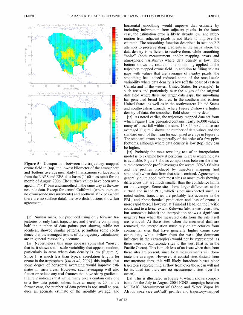
Figure 5. Comparison between the trajectory‐mappedozone field in (top) the lowest kilometer of the atmosphereand (bottom) average mean daily 1 h maximum surface ozonefrom the NAPS and EPA data bases (1160 sites total) for themonth of August 2006. The surface values have been aver-aged in 1° × 1° bins and smoothed in the same way as the ozo-nesonde data. Except for central California (where there areno ozonesonde measurements) and northern Mexico (wherethere are no surface data), the two distributions show fairagreement.

TARASICK ET AL.: TROPOSPHERIC OZONE FIELDS FROM IONS D20301D20301

7 of 12

ozone (not smoothed) at four sites in eastern North America.Differences below 10 km are generally within 95% confi-dence limits on the averages, except for Atlanta. Atlanta ison the coast, and the nearest sounding sites (Houston andHuntsville) are quite distant and inland.[25] Figure 5 shows a comparison between the (smoothed)

trajectory‐mapped ozone field for 0–1 km and mean daily1 h maximum surface ozone from the National Air PollutionSurveillance (NAPS) network Canada‐wide data baseand the U.S. EPA Air Quality System (AQS) data base(1160 sites total) during the month of August 2006. Meandaily 1 h maximum ozone was chosen as the parameter mostsimilar to the ozone soundings, as the latter were mostlytaken in midafternoon. The surface values have been aver-aged in 1° × 1° bins and smoothed in the same way as theozonesonde data. The 0–1 km layer is only approximatelyrepresentative of the PBL, and as remarked above, trajectoryerrors in the PBL are expected to be larger than in the freetroposphere. The surface data are also highly concentrated inCalifornia and the eastern United States and sparse throughthe midwestern United States and Canada; errors in thesurface field will be primarily due to linear interpolation inregions of sparse data. Despite these caveats, except forcentral California (where there are no ozonesonde mea-

surements) and northern Mexico (where there are no surfacedata), the distribution patterns show evident similarities. Amore quantitative comparison, selecting pixels that containboth several surface sites and several trajectory‐mappedozone values (not smoothed), shows a correlation coefficientof about 0.6 for the August 2006 period, if the centralCalifornia values are excluded. Similar comparisons for theother IONS periods show correlation coefficients generallybetween 0.6 and 0.7, with the exception of spring 2006,for which the correlation is poor (0.2).

3.2. Examples

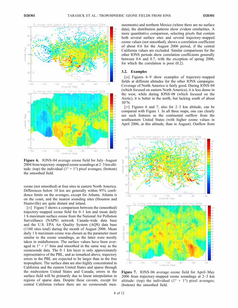
[26] Figures 6–9 show examples of trajectory‐mappedfields at different altitudes for the other IONS campaigns.Coverage of North America is fairly good. During IONS‐04(which focused on eastern North America), it is less dense inthe west, while during IONS‐08 (which focused on theArctic), it is better in the north, but lacking south of about30°N.[27] Figures 6 and 7, also for 2–3 km altitude, can be

compared with Figure 1. In all three maps, one can clearlysee such features as the continental outflow from thesoutheastern United States (with higher ozone values inApril 2006, at this altitude, than in August). Outflow from

Figure 7. IONS‐06 average ozone field for April–May2006 from trajectory‐mapped ozone soundings at 2–3 kmaltitude: (top) the individual (1° × 1°) pixel averages;(bottom) the smoothed field.

Figure 6. IONS‐04 average ozone field for July–August2004 from trajectory‐mapped ozone soundings at 2–3 kmalti-tude: (top) the individual (1° × 1°) pixel averages; (bottom)the smoothed field.

TARASICK ET AL.: TROPOSPHERIC OZONE FIELDS FROM IONS D20301D20301

8 of 12

the northeastern United States and Canada is also evident inall three maps, but this has higher values in August 2006,and possibly in both summers. However, there is limitedsampling off the east coast of Canada in the spring 2006map (Figure 7), resulting in a smoother field that may beexaggerating the value of these sparse data.[28] The outflow off the California coast in August 2006

(Figure 1) is present but weaker in 2004 and apparentlystronger (more data points further from land) but with lowerozone on average in April to May 2006. In both of thesummer figures a number of pixels with ozone values of70–75 ppb off the coast of California have been interpo-lated in the smoothed plot to a large and prominent feature,quite possibly exaggerating its importance. Also, in all threefigures, features appear to be “stretched” by the smoothingon the edges of the sampling domain, most evidently towardthe south. This is again an artifact of the smoothing, whichfills in data gaps with the nearest available information. Thehigh ozone feature off the Mexican coast in August 2006 isnot seen in other maps, but this is likely because there wereno Mexico City ozone soundings in the other data sets.[29] The eastern continental outflow is much less evi-

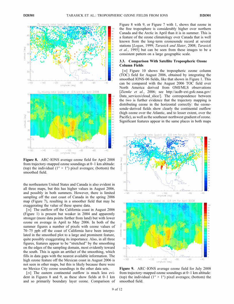
dent in Figures 8 and 9, as these show fields at 0–1 kmand so primarily boundary layer ozone. Comparison of

Figure 8 with 9, or Figure 7 with 1, shows that ozone inthe free troposphere is considerably higher over northernCanada and the Arctic in April than it is in summer. This isa feature of the ozone climatology over Canada that is wellknown from the long‐term ozonesonde record at severalstations [Logan, 1999; Tarasick and Slater, 2008; Tarasicket al., 1995] but can be seen from these images to be aconsistent pattern on a large geographic scale.

3.3. Comparison With Satellite Tropospheric OzoneColumn Fields

[30] Figure 10 shows the tropospheric ozone column(TOC) field for August 2006, obtained by integrating thesmoothed IONS‐06 fields, like that shown in Figure 1. Thiscan be compared with the August 2006 TOC field overNorth America derived from OMI/MLS observations[Ziemke et al., 2006; see http://acdb‐ext.gsfc.nasa.gov/Data_services/cloud_slice/]. The correspondence betweenthe two is further evidence that the trajectory mapping isdistributing ozone in the horizontal correctly: the ozone-sonde‐derived fields show clearly the continental outflow(high ozone over the Atlantic, and to lesser extent, over thePacific), as well as the southeast‐northwest gradient of ozone.Significant features appear in the same places in both maps

Figure 9. ARC‐IONS average ozone field for July 2008from trajectory‐mapped ozone soundings at 0–1 km altitude:(top) the individual (1° × 1°) pixel averages; (bottom) thesmoothed field.

Figure 8. ARC‐IONS average ozone field for April 2008from trajectory‐mapped ozone soundings at 0–1 km altitude:(top) the individual (1° × 1°) pixel averages; (bottom) thesmoothed field.

TARASICK ET AL.: TROPOSPHERIC OZONE FIELDS FROM IONS D20301D20301

9 of 12

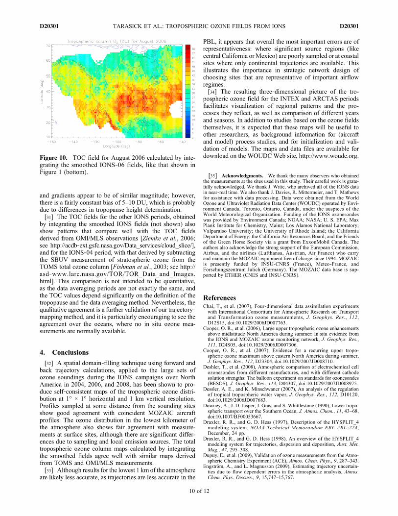
and gradients appear to be of similar magnitude; however,there is a fairly constant bias of 5–10 DU, which is probablydue to differences in tropopause height determination.[31] The TOC fields for the other IONS periods, obtained

by integrating the smoothed IONS fields (not shown) alsoshow patterns that compare well with the TOC fieldsderived from OMI/MLS observations [Ziemke et al., 2006;see http://acdb‐ext.gsfc.nasa.gov/Data_services/cloud_slice/],and for the IONS‐04 period, with that derived by subtractingthe SBUV measurement of stratospheric ozone from theTOMS total ozone column [Fishman et al., 2003; see http://asd‐www.larc.nasa.gov/TOR/TOR_Data_and_Images.html]. This comparison is not intended to be quantitative,as the data averaging periods are not exactly the same, andthe TOC values depend significantly on the definition of thetropopause and the data averaging method. Nevertheless, thequalitative agreement is a further validation of our trajectory‐mapping method, and it is particularly encouraging to see theagreement over the oceans, where no in situ ozone mea-surements are normally available.

4. Conclusions

[32] A spatial domain‐filling technique using forward andback trajectory calculations, applied to the large sets ofozone soundings during the IONS campaigns over NorthAmerica in 2004, 2006, and 2008, has been shown to pro-duce self‐consistent maps of the tropospheric ozone distri-bution at 1° × 1° horizontal and 1 km vertical resolution.Profiles sampled at some distance from the sounding sitesshow good agreement with coincident MOZAIC aircraftprofiles. The ozone distribution in the lowest kilometer ofthe atmosphere also shows fair agreement with measure-ments at surface sites, although there are significant differ-ences due to sampling and local emission sources. The totaltropospheric ozone column maps calculated by integratingthe smoothed fields agree well with similar maps derivedfrom TOMS and OMI/MLS measurements.[33] Although results for the lowest 1 km of the atmosphere

are likely less accurate, as trajectories are less accurate in the

PBL, it appears that overall the most important errors are ofrepresentativeness: where significant source regions (likecentral California or Mexico) are poorly sampled or at coastalsites where only continental trajectories are available. Thisillustrates the importance in strategic network design ofchoosing sites that are representative of important airflowregimes.[34] The resulting three‐dimensional picture of the tro-

pospheric ozone field for the INTEX and ARCTAS periodsfacilitates visualization of regional patterns and the pro-cesses they reflect, as well as comparison of different yearsand seasons. In addition to studies based on the ozone fieldsthemselves, it is expected that these maps will be useful toother researchers, as background information for (aircraftand model) process studies, and for initialization and vali-dation of models. The maps and data files are available fordownload on the WOUDCWeb site, http://www.woudc.org.

[35] Acknowledgments. We thank the many observers who obtainedthe measurements at the sites used in this study. Their careful work is grate-fully acknowledged. We thank J. Witte, who archived all of the IONS datain near‐real time. We also thank J. Davies, R. Mittermeier, and T. Mathewsfor assistance with data processing. Data were obtained from the WorldOzone and Ultraviolet Radiation Data Center (WOUDC) operated by Envi-ronment Canada, Toronto, Ontario, Canada, under the auspices of theWorld Meteorological Organization. Funding of the IONS ozonesondeswas provided by Environment Canada; NOAA; NASA; U. S. EPA; MaxPlank Institute for Chemistry, Mainz; Los Alamos National Laboratory;Valparaiso University; the University of Rhode Island; the CaliforniaDepartment of Energy; the California Air Resources Board; and the Friendsof the Green Horse Society via a grant from ExxonMobil Canada. Theauthors also acknowledge the strong support of the European Commission,Airbus, and the airlines (Lufthansa, Austrian, Air France) who carryand maintain the MOZAIC equipment free of charge since 1994. MOZAICis presently funded by INSU‐CNRS (France), Meteo‐France, andForschungszentrum Julich (Germany). The MOZAIC data base is sup-ported by ETHER (CNES and INSU‐CNRS).

ReferencesChai, T., et al. (2007), Four‐dimensional data assimilation experimentswith International Consortium for Atmospheric Research on Transportand Transformation ozone measurements, J. Geophys. Res., 112,D12S15, doi:10.1029/2006JD007763.

Cooper, O. R., et al. (2006), Large upper tropospheric ozone enhancementsabove midlatitude North America during summer: In situ evidence fromthe IONS and MOZAIC ozone monitoring network, J. Geophys. Res.,111, D24S05, doi:10.1029/2006JD007306.

Cooper, O. R., et al. (2007), Evidence for a recurring upper tropo-spheric ozone maximum above eastern North America during summer,J. Geophys. Res., 112, D23304, doi:10.1029/2007JD008710.

Deshler, T., et al. (2008), Atmospheric comparison of electrochemical cellozonesondes from different manufactures, and with different cathodesolution strengths: The balloon experiment on standards for ozonesondes(BESOS), J. Geophys. Res., 113, D04307, doi:10.1029/2007JD008975.

Dessler, A. E., and K. Minschwaner (2007), An analysis of the regulationof tropical tropospheric water vapor, J. Geophys. Res., 112, D10120,doi:10.1029/2006JD007683.

Downey, A., J. D. Jasper, J. Gras, and S. Whittlestone (1990), Lower tropo-spheric transport over the Southern Ocean, J. Atmos. Chem., 11, 43–68,doi:10.1007/BF00053667.

Draxler, R. R., and G. D. Hess (1997), Description of the HYSPLIT_4modeling system, NOAA Technical Memorandum ERL ARL‐224,December, 24 pp.

Draxler, R. R., and G. D. Hess (1998), An overview of the HYSPLIT_4modeling system for trajectories, dispersion and deposition, Aust. Met.Mag., 47, 295–308.

Dupuy, E., et al. (2009), Validation of ozone measurements from the Atmo-spheric Chemistry Experiment (ACE), Atmos. Chem. Phys., 9, 287–343.

Engström, A., and L. Magnusson (2009), Estimating trajectory uncertain-ties due to flow dependent errors in the atmospheric analysis, Atmos.Chem. Phys. Discuss., 9, 15,747–15,767.

Figure 10. TOC field for August 2006 calculated by inte-grating the smoothed IONS‐06 fields, like that shown inFigure 1 (bottom).

TARASICK ET AL.: TROPOSPHERIC OZONE FIELDS FROM IONS D20301D20301

10 of 12

Fishman, J., A. E. Wozniak, and J. K. Creilson (2003), Global distributionof tropospheric ozone from satellite measurements using the empiricallycorrected tropospheric ozone residual technique: Identification of theregional aspects of air pollution, Atmos. Chem. Phys., 3, 893–907,doi:10.5194/acp-3-893-2003.

Harris, J. M., R. R. Draxler, and S. J. Oltmans (2005), Trajectory modelsensitivity to differences in input data and vertical transport method,J. Geophys. Res., 110, D14109, doi:10.1029/2004JD005750.

Jerrett, M., R. T. Burnett, C. A. Pope III, K. Ito, G. Thurston, D. Krewski,Y. Shi, E. Calle, and M. Thun (2009), Long‐term ozone exposure andmortality, N. Engl. J. Med., 360, 1085–1095.

Jiang, Y., et al. (2007), Validation of aura microwave limb sounder ozoneby ozonesonde and lidar measurements, J. Geophys. Res., 112, D24S34,doi:10.1029/2007JD008776.

Kerr, J. B., et al. (1994), The 1991 WMO international ozonesonde inter-comparison at Vanscoy, Canada, Atmos.‐Ocean, 32, 685–716.

Liu, G., D. W. Tarasick, V. E. Fioletov, C. E. Sioris, and Y. J. Rochon(2009), Ozone correlation lengths and measurement uncertainties fromanalysis of historical ozonesonde data in North America and Europe,J. Geophys. Res., 114, D04112, doi:10.1029/2008JD010576.

Liu, X., K. Chance, C. E. Sioris, R. J. D. Spurr, T. P. Kurosu, R. V. Martin,and M. J. Newchurch (2005), Ozone profile and tropospheric ozone retrie-vals from the Global Ozone Monitoring Experiment: Algorithm descrip-tion and validation, J. Geophys. Res., 110, D20307, doi:10.1029/2005JD006240.

Liu, X., P. K. Bhartia, K. Chance, R. J. D. Spurr, and T. P. Kurosu (2009a),Ozone profile retrievals from the Ozone Monitoring Instrument, Atmos.Chem. Phys. Discuss., 9, 22,693–22,738.

Liu, X., P. K. Bhartia, K. Chance, T. P. Kurosu, and R. J. D. Spurr (2009b),Validation of OMI ozone profiles and stratospheric ozone columns withmicrowave limb sounder, Atmos. Chem. Phys. Discuss., 9, 24,913–24,943.

Livingston, J., et al. (2007), Comparison of water vapor measurements byairborne Sun photometer and near‐coincident in situ and satellite sensorsduring INTEX/ITCT 2004, J. Geophys. Res., 112, D12S16, doi:10.1029/2006JD007733.

Logan, J. A. (1999), An analysis of ozonesonde data for the troposphere:Recommendations for testing 3‐D models and development of a griddedclimatology for tropospheric ozone, J. Geophys. Res., 104(D13),16,115–16,149, doi:10.1029/1998JD100096.

Mao, H., R. Talbot, D. Troop, R. Johnson, S. Businger, and A.M. Thompson(2006), Smart balloon observations over the North Atlantic: O3 data anal-ysis and modeling, J. Geophys. Res., 111, D23S56, doi:10.1029/2005JD006507.

Merrill, J., R. Bleck, and L. Avila (1985), Modeling Atmospheric Transportto the Marshall Islands, J. Geophys. Res., 90(D7), 12,927–12,936,doi:10.1029/JD090iD07p12927.

Methven, J., S. R. Arnold, F. M. O’Connor, H. Barjat, K. Dewey, J. Kent,and N. Brough (2003), Estimating photochemically produced ozonethroughout a domain using flight data and a Lagrangianmodel, J. Geophys.Res., 108(D9), 4271, doi:10.1029/2002JD002955.

Morris, G. A., J. F. Gleason, J. Ziemke, and M. R. Schoeberl (2000), Trajec-tory mapping: A tool for validation of trace gas observations, J. Geophys.Res., 105(D14), 17,875–17,894, doi:10.1029/1999JD901118.

Nardi, B., et al. (2008), Initial validation of ozone measurements from theHigh Resolution Dynamics Limb Sounder, J. Geophys. Res., 113,D16S36, doi:10.1029/2007JD008837.

Nassar, R., et al. (2008), Validation of tropospheric emission spectrometer(TES) Nadir ozone profiles using ozonesonde measurements, J. Geophys.Res., 113, D15S17, doi:10.1029/2007JD008819.

Newman, P. A., and M. R. Schoeberl (1995), A reinterpretation of the datafrom the NASA Stratosphere‐Troposphere Exchange Project, Geophys.Res. Lett., 22(18), 2501–2504, doi:10.1029/95GL02220.

Parrington, M., D. B. A. Jones, K. W. Bowman, L. W. Horowitz, A. M.Thompson, D. Tarasick, and J. C. Witte (2008), Constraining the sum-mertime tropospheric ozone distribution over North America throughassimilation of observations from the Tropospheric Emission Spectrom-eter, J. Geophys. Res., 113, D18307, doi:10.1029/2007JD009341.

Parrington, M., D. B. A. Jones, K. W. Bowman, A. M. Thompson, D. W.Tarasick, J. Merrill, S. J. Oltmans, T. Leblanc, J. C.Witte, and D. B. Millet(2009), Impact of the assimilation of ozone from the Tropospheric Emis-sion Spectrometer on surface ozone across North America, Geophys.Res. Lett., 36, L04802, doi:10.1029/2008GL036935.

Pfister, G. G., L. K. Emmons, P. G. Hess, J.‐F. Lamarque, A. M. Thompson,and J. E. Yorks (2008), Analysis of the Summer 2004 ozone budget overthe United States using Intercontinental Transport Experiment Ozone-sonde Network Study (IONS) observations and Model of Ozone andRelated Tracers (MOZART‐4) simulations, J. Geophys. Res., 113,D23306, doi:10.1029/2008JD010190.

Pierce, R. B., et al. (2007), Chemical data assimilation estimates of conti-nental U. S. ozone and nitrogen budgets during the IntercontinentalChemical Transport Experiment–North America, J. Geophys. Res.,112, D12S21, doi:10.1029/2006JD007722.

Pierce, R. B., et al. (2009), Impacts of background ozone production onHouston and Dallas, Texas, air quality during the Second Texas AirQuality Study field mission, J. Geophys. Res. , 114 , D00F09,doi:10.1029/2008JD011337.

Pierrehumbert, R. (1998), Lateral mixing as a source of subtropical watervapor, Geophys. Res. Lett., 25(2), 151–154, doi:10.1029/97GL03563.

Pierrehumbert, R., and R. Roca (1998), Evidence for control of Atlanticsubtropical humidity by large scale advection, Geophys. Res. Lett., 25(24),4537–4540, doi:10.1029/1998GL900203.

Roelofs, G.‐J., and J. Lelieveld (1997), Model study of the influence ofcross‐tropopause O3 transports on tropospheric O3 levels, Tellus Ser. B,49, 38–55.

Schoeberl, M. R., et al. (2007), A trajectory based estimate of the tropo-spheric column ozone column using the residual method, J. Geophys.Res., 112, D24S49, doi:10.1029/2007JD008773.

Smit, H. G. J., et al. (2007), Assessment of the performance of ECC‐ozonesondes under quasi‐flight conditions in the environmental simula-tion chamber: Insights from the Juelich Ozone Sonde IntercomparisonExperiment (JOSIE), J. Geophys. Res., 112, D19306, doi:10.1029/2006JD007308.

Stajner, I., et al. (2008), Assimilated ozone from EOS‐Aura: Evaluation ofthe tropopause region and tropospheric columns, J. Geophys. Res., 113,D16S32, doi:10.1029/2007JD008863.

Stevenson, D. S., et al. (2006), Multimodel ensemble simulations of presentday and near‐future tropospheric ozone, J. Geophys. Res., 111, D08301,doi:10.1029/2005JD006338.

Stohl, A. (1998), Computation, accuracy and applications of trajectories –A review and bibliography, Atmos. Environ., 32, 947–966.

Stohl, A., and P. Seibert (1997), Accuracy of trajectories as determinedfrom the conservation of meteorological tracers, Q. J. R. Meteorol.Soc., 124, 1465–1484, doi:10.1002/qj.49712454907.

Stohl, A., P. James, C. Forster, N. Spichtinger, A. Marenco, V. Thouret,and H. G. J. Smit (2001), An extension of Measurement of Ozone andWater Vapour by Airbus In‐service Aircraft (MOZAIC) ozone climatol-ogies using trajectory statistics, J. Geophys. Res., 106, 27,757–27,768,doi:10.1029/2001JD000749.

Sutton, R. T., H. Maclean, R. Swinbank, A. O’Neill, and F. W. Taylor(1994), High‐resolution stratospheric tracer fields estimated from satelliteobservations using Lagrangian trajectory calculations, J. Atmos. Sci., 51,2995–3005.

Tang, Y., et al. (2008), The impact of chemical lateral boundary conditionson CMAQ predictions of tropospheric ozone over the continental UnitedStates, Environ. Fluid Mech., 9, 43–58, doi:10.1007/s10652-008-9092-5.

Tarasick, D. W., and R. Slater (2008), Ozone in the troposphere: Measure-ments, climatology, budget, and trends, Atmos.‐Ocean, 46, 93–115,doi:10.3137/ao.460105.

Tarasick, D. W., D. I. Wardle, J. B. Kerr, J. J. Bellefleur, and J. Davies(1995), Tropospheric ozone trends over Canada: 1980–1993, Geophys.Res. Lett., 22(4), 409–412, doi:10.1029/94GL02991.

Tarasick, D. W., et al. (2007), Comparison of Canadian air quality fore-cast models with tropospheric ozone profile measurements above mid‐latitude North America during the IONS/ICARTT Campaign: Evidencefor stratospheric input, J. Geophys. Res., 112, D12S22, doi:10.1029/2006JD007782.

Thompson, A. M., et al. (2007a), Intercontinental chemical transport exper-iment Ozonesonde Network Study (IONS) 2004: 1. Summertime uppertroposphere/lower stratosphere ozone over northeastern North America,J. Geophys. Res., 112, D12S12, doi:10.1029/2006JD007441.

Thompson, A. M., et al. (2007b), Intercontinental chemical transport exper-iment Ozonesonde Network Study (IONS) 2004: 2. Tropospheric ozonebudgets and variability over northeastern North America, J. Geophys.Res., 112, D12S13, doi:10.1029/2006JD007670.

Thompson, A. M., J. E. Yorks, S. K. Miller, J. C. Witte, G. A. Morris,D. Baumgardner, L. Ladino, and B. Rappenglueck (2008), Troposphericozone sources and wave activity over Mexico City and Houston duringMilagro/Intercontinental Transport Experiment (INTEX‐B) OzonesondeNetwork Study, 2006 (IONS‐06), Atmos. Chem. Phys., 8, 5113–5125.

von Kuhlmann, R., M. G. Lawrence, P. J. Crutzen, and P. J. Rasch (2003),A model for studies of tropospheric ozone and nonmethane hydrocar-bons: Model description and ozone results, J. Geophys. Res., 108(D9),4294, doi:10.1029/2002JD002893.

World Meteorological Organization (1992), International meteorologicalvocabulary,WMO Rep. 182, World Meteorol. Org., Geneva, Switzerland.

TARASICK ET AL.: TROPOSPHERIC OZONE FIELDS FROM IONS D20301D20301

11 of 12

Yorks, J. E., A. M. Thompson, E. Joseph, and S. K. Miller (2009), The var-iability of free tropospheric ozone budgets over Beltsville, Maryland(39N, 77W) in the summers 2004–2007, Atmos. Environ., 43, 1827–1838.

Yu, S., R. Mathur, K. Schere, D. Kang, J. Pleim, and T. L. Otte (2007), Adetailed evaluation of the Eta‐CMAQ forecast model performance forO3, its related precursors, and meteorological parameters during the2004 ICARTT study, J. Geophys. Res., 112, D12S14, doi:10.1029/2006JD007715.

Ziemke, J. R., S. Chandra, B. N. Duncan, L. Froidevaux, P. K. Bhartia, P. F.Levelt, and J. W. Waters (2006), Tropospheric ozone determined fromAura OMI and MLS: Evaluation of measurements and comparison withthe Global Modeling Initiative’s Chemical Transport Model, J. Geophys.Res., 111, D19303, doi:10.1029/2006JD007089.

O. R. Cooper, Cooperative Institute for Research in EnvironmentalSciences, University of Colorado, Boulder, CO 80309, USA.T. Dann, Air Quality Research Division, Environment Canada, 335 River

Road, Ottawa, ON, Canada K1V 1C7.

V. E. Fioletov, J. Liu, C. E. Sioris, and D. W. Tarasick, Air QualityResearch Division, Environment Canada, Downsview, ON, Canada M3H5T4. ([email protected])J. J. Jin, Jet Propulsion Laboratory, California Institute of Technology,

4800 Oak Grove Drive, Mail Stop 183‐701, Pasadena, CA 91109, USA.G. Liu, Space Sciences Laboratory, 7 Gauss Way 7450, University of

California, Berkeley, CA 94720‐7450, USA.X. Liu, Goddard Earth Sciences and Technology Center, University of

Maryland, Baltimore County, 5523 Research Park Drive, Suite 320,Baltimore, MD 21228, USA.S. J. Oltmans, NOAA Climate Monitoring and Diagnostics Laboratory,

325 Broadway, Boulder, CO 80305, USA.A. M. Thompson, Department of Meteorology, 510 Walker Building,

Pennsylvania State University, University Park, PA 16802, USA.V. Thouret, Laboratoire d’Aerologie, Centre National de la Recherche

Scientifique, Observatoire Midi‐Pyrenees, 14 Av. E. Belin, 31400,Toulouse, France.

TARASICK ET AL.: TROPOSPHERIC OZONE FIELDS FROM IONS D20301D20301

12 of 12