High-resolution numerical modeling of wave-supported gravity-driven mudflows

High-resolution numerical modeling of wave-supported

gravity-driven mudflows

Tian-Jian Hsu,1 Celalettin E. Ozdemir,2 and Peter A. Traykovski3

Received 7 July 2008; revised 30 October 2008; accepted 19 March 2009; published 14 May 2009.

[1] Wave-supported gravity-driven mudflow has been identified as a major offshore finesediment transport mechanism of terrestrial sediment into the coastal ocean. This transportprocess essentially occurs within the wave boundary layer. In this study, wave-supportedgravity-driven mudflow is investigated via a wave-phase-resolving high-resolutionnumerical model for fluid mud transport. The model results are verified with fieldobservation of sediment concentration and near-bed flow velocities at Po prodelta. Thecharacteristics of wave-supported gravity-driven mudflows are diagnosed by varying thebed erodibility, floc properties (fractal dimension), and rheological stresses in thenumerical simulations. Model results for moderate concentration suggest that using anappropriately specified fractal dimension, the dynamics of wave-supported gravity-drivenmudflow can be predicted without explicitly incorporating rheological stress. However,incorporating rheological stress makes the results less sensitive to prescribed fractaldimension. For high-concentration conditions, it is necessary to incorporate rheologicalstress in order to match observed intensity of downslope gravity-driven current. Modelresults are further analyzed to evaluate and calibrate simple parameterizations. Analysissuggests that when neglecting rheological stress, the drag coefficient decreases withincreasing wave intensity and seems to follow a power law. However, when rheologicalstress is incorporated, the resulting drag coefficient is more or less constant (around0.0013) for different wave intensities. Model results further suggest the bulk Richardsonnumber has a magnitude smaller than 0.25 and is essentially determined by the amount ofavailable soft mud (i.e., the erodibility), suggesting a supply limited condition forunconsolidated mud.

Citation: Hsu, T.-J., C. E. Ozdemir, and P. A. Traykovski (2009), High-resolution numerical modeling of wave-supported gravity-

driven mudflows, J. Geophys. Res., 114, C05014, doi:10.1029/2008JC005006.

1. Introduction

[2] It is important to understand the fate of terrestrialsediment into the coastal ocean, because it determines forexample the seabed properties and long-term coastal geo-morphology [e.g., Wright and Coleman, 1972; Syvitski etal., 1988; Friedrichs and Wright, 2004]. The world’s fluvialshelf system can be classified into several contrasting cases[e.g., Wright and Nittrouer, 1995]. However, for sedimenttransport we can generally consider the fluvial shelf systemas either large rivers discharging into passive margins (ormarginal seas) with relatively wide continental shelf, suchas the Amazon shelf; or small mountainous rivers attectonically active mountain belts that directly dischargeinto active margins [Milliman and Syvitski, 1992]. Since the

study of Milliman and Syvitski [1992], the significance ofsmall mountainous river contributions to the world’s totalsediment discharge into the ocean has been emphasized.[3] Terrestrial sediments delivered by moderate to large

rivers are driven by seasonal variations. In contrast, forsmall mountainous river systems, major sedimentationevents are dominated by large rainfall events that occurover a short period of time [Wheatcroft, 2000]. In the mostextreme conditions, sediment delivery from small moun-tainous river mouths can generate episodic hyperpycnalplume because of their large sediment yield [Mulder andSyvitski, 1995; Wright and Nittrouer, 1995; Milliman et al.,2007]. In this case, hyperpycnal plume can carry largeamount of fluvial sediment away from the shore in arelatively short period of time [Imran and Syvitski, 2000].According to the analysis reported by Mulder and Syvitski[1995], except for several ‘‘dirty’’ mountainous rivers inthe world where the hyperpycnal plume may be triggeredby heavy rainfall due to typhoons or tropical cyclones onan annual basis [Milliman and Kao, 2005; Dadson et al.,2005], in most situations the initial deposition remainsrather close to the river mouth. For example, at EelRiver shelf of Northern California (USA) the probability

JOURNAL OF GEOPHYSICAL RESEARCH, VOL. 114, C05014, doi:10.1029/2008JC005006, 2009ClickHere

for

FullArticle

1Center for Applied Coastal Research, Civil and EnvironmentalEngineering, University of Delaware, Newark, Deleware, USA.

2Civil and Coastal Engineering, University of Florida, Gainesville,Florida, USA.

3Applied Ocean Physics and Engineering, Woods Hole OceanographicInstitution, Woods Hole, Massachusetts, USA.

Copyright 2009 by the American Geophysical Union.0148-0227/09/2008JC005006$09.00

C05014 1 of 15

http://dx.doi.org/10.1029/2008JC005006

of hyperpycnal plume occurrence is about once every100 years. During the STRATAFORM field experimentsat Eel River shelf [Nittrouer and Kravitz, 1996], the initialdepositions from the river plume are observed to be at theinner shelf within the 40 m isobath [Geyer et al., 2000].However, coring survey indicates that major flood depositsare found in the north of the river mouth in water depth of50–100 m [Wheatcroft and Borgeld, 2000]. Such offshoretransport of initially deposited terrestrial sediment must becaused by shelf resuspension processes. However, numer-ical modeling suggests that conventional resuspensionmechanisms due to energetic waves and currents cannotaccount for the observed offshore transport [Harris et al.,2004]. Hence, other offshore transport mechanisms inadditional to the conventional bottom boundary layerprocesses must be considered.[4] According to the criterion suggested for the occur-

rence of turbidity current [Parker, 1982], the slope of Eelshelf (or most other continental shelves) is too mild toinitiate autosuspending turbidity current for offshore sedi-ment transport [Wright et al., 2001]. Therefore, such down-slope gravity-driven transport has been associated withstrong wave-current resuspension. During the STRATA-FORM field experiment, direct measurements indicate thatthe concentration of the near-bed suspended sedimentexceed the level of fluid mud (�10 g/L) [Ogston et al.,2000; Traykovski et al., 2000]. Hence, it is possible thatsuch high sediment concentration may provide sufficientdensity anomaly to allow gravity-driven downslope mud-flows. This conjecture is further confirmed by the measurednear-bed flow velocity during fluid mud event that showsthe maximum downslope current velocity occurs near thelutocline, consistent with typical gravity-current profile[Traykovski et al., 2000]. Hence, a conceptual picture canbe described as follow. When there is sufficient amount ofunconsolidated fine sediment deposits available near rivermouth, they are resuspended by high bottom stress andboundary layer turbulence under energetic condition. Thepresence of a high-concentration sediment suspension fur-ther damps the carrier flow turbulence and can form a densefluid mud layer near the bed [Trowbridge and Kineke,1994], which may establish sufficient buoyancy anomalyto drive downslope gravitational transport. Apparently, theoccurrences of wave-supported gravity-driven mudflows arealso more frequent than previously believed. During theEuroSTRATAFORM program [Sherwood et al., 2004],wave-supported gravity-driven mudflow were also observedat Po River prodelta [Traykovski et al., 2007], which is aless energetic environment with a flatter slope than the EelRiver shelf.[5] Despite the critical role of downslope gravitational

force, wave-supported gravity-driven mudflows are essen-tially a bottom boundary layer fluid mud process. In atypical coastal modeling system [e.g., Lesser et al., 2004;Harris et al., 2005; Warner et al., 2008], the numericalmodel is not designed to resolve near-bed wave boundarylayer processes. In order to predict large-scale sedimenttransport and morphological evolution, wave-supportedgravity-driven mudflows have to be parameterized as partof the bottom boundary layer module [e.g., Harris et al.,2004, 2005]. Several prior studies propose simplified near-bed formulations for gravity-driven fluid mud transport in

the wave boundary layer [Wright et al., 2001; Harris et al.,2004; Fan et al., 2004] that can be coupled with coastalmodels. However, there are several critical assumptions inthese formulations and empirical coefficients that need to bedetermined.[6] Fluid mud resuspension processes in the wave-current

bottom boundary layer can be predicted by detailed watercolumn numerical model for fluid velocity and sedimentconcentration provided that appropriate turbulence closureand bottom boundary conditions are incorporated [Wiberg etal., 1994; van der Ham and Winterwerp, 2001; Hsu et al.,2007]. Using these small-scale models, it has been shownthat with adequate supply of fine sediment that can beresuspended, the most important mechanism to predict theexistence of fluid mud is the effect of sediment on dampingthe carrier flow turbulence. These numerical model resultsare consistent with earlier theoretical analysis and experi-mental evidence [Wolanski et al., 1988; Trowbridge andKineke, 1994; Vinzon and Mehta, 1998]. Recently, Hsu etal. [2007] developed a numerical model for fine sedimenttransport. In this fine transport modeling framework, mech-anisms such as rheological stresses, gravity-driven sedimentflow and turbulence modulation by the presence of sedimentare incorporated consistently in a formulation simplifiedfrom the multiphase flow theory by assuming small particleresponse time. They demonstrated that the new fine sedi-ment transport model is able to predict the existence of fluidmud and subsequent downslope gravity-driven transportwhen driven by realistic cross-shelf and along-shelf near-bed wave-current velocities measured at Po River prodelta[Traykovski et al., 2007].[7] Our current understanding on the dynamic of fluid

mud processes in the wave boundary layer is limited. This ispartially due to the difficulties in accurate measurement onturbulence, floc properties, rheology and erodibility inconcentrated regime. Because the fluid mud model previ-ously developed by Hsu et al. [2007] resolves the waveboundary layer, incorporates the damping of turbulence dueto sediment in the k-e equations, and allows sedimentconcentration to drive gravitational flow in the momentumequations, the authors demonstrate that the model is able topredict observed wave-supported gravity-driven mudflowswithout explicitly incorporating more sophisticated cohe-sive sediment characteristics. However, without explicitlyincorporating cohesive sediment characteristics, it is diffi-cult to fully understand and quantify the fluid mud transportprocesses. The purpose of this study is twofold. First, thenumerical model of Hsu et al. [2007] is revised to incor-porate several well-known cohesive sediment characteristicsin order to study their effects on wave-supported gravity-driven mudflows (section 3). Second, typical coastal mod-eling systems for morphodynamics cannot resolve processesoccur within the wave boundary layer and hence theseprocesses must be parameterized. Numerical model resultsare further analyzed (section 4) to evaluate the empiricalparameters used in a 1-D depth-integrated parameterizationof wave-supported gravity-driven mudflows suggested byWright et al. [2001; see also Wright and Friedrichs, 2006].[8] This paper is organized as follow. Model formulation

is discussed in section 2. Specifically, we focus on severalnew revisions to the model that are unique for cohesivesediment. In section 3, the capability of the numerical model

C05014 HSU ET AL.: WAVE-SUPPORTED GRAVITY-DRIVEN MUDFLOWS

2 of 15

C05014

is demonstrated by comparing the model results with field datameasured at Po prodelta when wave-supported gravity-drivenmudflows are observed under two different conditions[Traykovski et al., 2007]. The nature and existence of wave-supported gravity-driven mudflows are further diagnosed byvarying the floc properties, bed erodibility, rheological stressesand along-shelf current intensity. In section 4, we investigatethe parameterization of wave-supported gravity-driven mud-flow [e.g.,Wright et al., 2001], specifically the dependence ofdrag coefficients and bulk Richardson numbers on the waveintensity. This study is concluded in section 5.

2. Numerical Model for Fluid Mud Transport

2.1. Model Formulation

[9] A 1DV wave-phase-resolving fine sediment transportmodel [Hsu et al., 2007] is revised here to simulate wave-supported gravity-driven mudflows in consideration of thecharacteristics of cohesive sediment. The governing equa-tion of the model is based on the Fast Equilibrium Eulerianapproximation [Ferry and Balachandar, 2001] to the Euler-ian two-phase equations. The characteristics of fluid-particleinteraction can be quantified by the particle response time[e.g., Allen, 1985; Ferry and Balachandar, 2001]:

Tp ¼raD2

18mf fð Þ ð1Þ

where ra is the particle (floc) density, D is the particle (floc)diameter, m is the dynamic viscosity of the interstitial fluid,and f(f) is a function representing hindered settling and is afunction of the particle (floc) volume concentration 8. Forthe fine floc particles considered in this paper, we set f(f) =(1 � f)4 [Richardson and Zaki, 1954]. Qualitatively,Tp represents the timescale required to accelerate a particle(floc) from rest to the velocity of the carrier fluid flow andis proportional to D2. Because the Fast EquilibriumEulerian approximation requires that the particle responsetime to be small, the present model is appropriate for finesediment (e.g., D < O(100) mm) transport in water.[10] We consider fluid mud transport in the bottom wave-

current boundary layer that is statistically homogeneous in

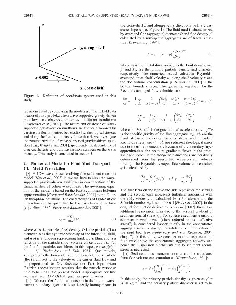
the cross-shelf x and along-shelf y directions with a cross-shore slope a (see Figure 1). The fluid mud is characterizedby averaged floc (aggregate) diameter D and floc density ra

calculated by assuming the aggregates are of fractal struc-ture [Kranenburg, 1994]:

ra ¼ rþ rs � rð Þ D

D0

� �nf �3

ð2Þ

where nf is the fractal dimension, r is the fluid density, andrs and D0 are the primary particle density and diameter,respectively. The numerical model calculates Reynolds-averaged cross-shelf velocity u, along-shelf velocity v andthe floc volume concentration 8 [Hsu et al., 2007] in thebottom boundary layer. The governing equations for theReynolds-averaged flow velocities are:

@u

@t¼ � 1

r@p

@xþ 1

r 1� fð Þ@t f

xz

@zþ @tsxz

@z

� �þ s� 1ð Þf

1� fð Þ g sina ð3Þ

@v

@t¼ � 1

r@p

@yþ 1

r 1� fð Þ@t f

yz

@zþ@tsyz@z

!ð4Þ

where g = 9.8 m/s2 is the gravitational acceleration, s = ra/ris the specific gravity of the floc aggregate, txz

f , tyzf are the

fluid stresses, including viscous stress and turbulentReynolds stress, and txz

s , tyzs are sediment rheological stress

due to interfloc interactions. Because of the boundary layerapproximation, the pressure gradients @p/@x in the cross-shelf and @p/@y in the along-shelf directions are iterativelydetermined from the prescribed wave-current velocityforcing. The Reynolds-averaged floc volume concentration8 is calculated by

@f@t

¼ @

@zfTp 1� s�1� �

g þ ntsf

@f@z

� �ð5Þ

The first term on the right-hand side represents the settlingand the second term represents turbulent suspension withthe eddy viscosity nt calculated by a k-e closure and theSchmidt number s8 is set to be 0.5 [Hsu et al., 2007]. In theoriginal formulation derived by Hsu et al. [2007], there is anadditional suspension term due to the vertical gradient ofsediment normal stress tzz

s . For cohesive sediment transport,sediment normal stress (often referred to as ‘‘effectivestress’’) is considered important only in the concentratedaggregate network during consolidation or fluidization ofthe mud bed [see Winterwerp and van Kesteren, 2004,chap. 7]. In this study, we consider mobile suspensions offluid mud above the concentrated aggregate network andhence the suspension mechanism due to sediment normalstress is neglected.[11] Sediment mass concentration c can be calculated

from floc volume concentration as [Kranenburg, 1994]:

c ¼ rsfD

D0

� �nf �3

¼ rsfra � rrs � r

� �ð6Þ

In this study, the primary particle density is given as rs =2650 kg/m3 and the primary particle diameter is set to be

Figure 1. Definition of coordinate system used in thisstudy.


3 of 15

C05014

D0 = 4 mm. In this paper, the floc diameter and fractaldimension are prescribed as constant. Hence, the dynamicsof floc break up and aggregation in turbulent flow are notexplicitly considered.[12] The fluid shear stresses consist of viscous and

turbulent Reynolds stresses. The turbulent Reynolds stressesare calculated by eddy viscosity and a k�e closure which ismodified for suspended sediment transport:

t fxz ¼ r f n þ ntð Þ @u

@z; t f

yz ¼ r f n þ ntð Þ @v@z

ð7Þ

with n the fluid viscosity, and the eddy viscosity nt iscalculated by turbulent kinetic energy k and its dissipationrate e:

nt ¼ Cmk2

e1� fð Þ: ð8Þ

The turbulent kinetic energy, k, and dissipation rate, e, areestimated by their balance equations

1� fð Þ @k@t

¼ nt@u

@z

� �2

þ @v

@z

� �2" #

þ @

@zn þ nt

sk

� �@ 1� fð Þk

@z

� 1� fð Þeþ s� 1ð Þg ntsc

@f@z

� 2fskTp þ TL

ð9Þ

and

1� fð Þ @e@t

¼ Ce1eknt

@u

@z

� �2

þ @v

@z

� �2" #

þ @

@zn þ nt

se

� �@ 1� fð Þe

@z

� Ce2

e2

k1� fð Þ

þ Ce3ek

s� 1ð Þg ntsc

@f@z

� 2fskTp þ TL

: ð10Þ

Balance equations (9) and (10) herein have two additionalterms compared to that of clear fluid. These terms representthe effects of fine sediment on carrier flow turbulence.Damping of turbulent kinetic energy due to sedimentdensity stratification is accounted for in the fourth term ofthe right-hand side in equation (9). In addition, dissipationin carrier fluid turbulence caused by viscous drag ofparticles in the fluctuating field is included the last term ofequation (9). This term is determined by using particleresponse time Tp, and turbulent eddy timescale TL, which iscalculated as:

TL ¼ k

6eð11Þ

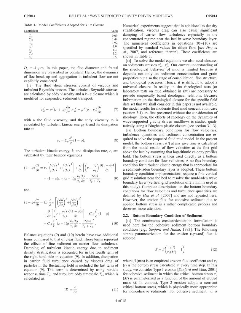
Numerical experiments suggest that in additional to densitystratification, viscous drag can also cause significantdamping of carrier flow turbulence especially in theconcentrated regime near the bed in wave boundary layer.The numerical coefficients in equations (8)–(10) arespecified by standard values for dilute flow [see Hsu etal., 2007, and reference therein]. These coefficients areshown in Table 1.[13] To solve the model equations we also need closures

on sediments stresses txzs , tyz

s . Our current understanding ofthe rheological behavior of mud is limited because itdepends not only on sediment concentration and grainproperties but also the stage of consolidation, floc structure,and biological processes. Hence, it is difficult to adopt auniversal closure. In reality, in situ rheological tests (orlaboratory tests on mud obtained in situ) are necessary toprovide empirically based rheological relations. Becauseinformation on the rheological closure for the specific fielddata set that we shall consider in this paper is not available,the model results for moderate fluid mud concentration case(section 3.1) are first presented without the consideration ofrheology. Then, the effects of rheology on the dynamics ofwave-supported gravity driven mudflows is studied quali-tatively using a Bingham plastic closure (see section 3.1.3).[14] Bottom boundary conditions for flow velocities,

turbulence quantities and sediment concentration are re-quired to solve the proposed fluid mud model. In the presentmodel, the bottom stress tb(t) at any give time is calculatedfrom the model results of flow velocities at the first gridabove the bed by assuming that logarithmic velocity profileshold. The bottom stress is then used directly as a bottomboundary condition for flow velocities. A no-flux boundarycondition for turbulent kinetic energy that is appropriate fora sediment-laden boundary layer is adopted. These bottomboundary condition implementations require a fine verticalgrid resolution near the bed to resolve the mud-laden waveboundary layer (vertical grid resolution of 2.5 mm is used inthis study). Complete descriptions on the bottom boundaryconditions for flow velocities and turbulence quantities aredetailed by Hsu et al. [2007] and are not repeated here.However, the erosion flux for cohesive sediment due toapplied bottom stress is a rather complicated process anddeserves more attention.

2.2. Bottom Boundary Condition of Sediment

[15] The continuous erosion/deposition formulation isused here for the cohesive sediment bottom boundarycondition [e.g., Sanford and Halka, 1993]. The followingsimple parameterization for the erosion (upward) flux isadopted:

E ¼ btb tð Þtc Mð Þ � 1

� �ð12Þ

where b (m/s) is an empirical erosion flux coefficient and tb(t) is the bottom stress calculated at every time step. In thisstudy, we consider Type 1 erosion [Sanford and Maa, 2001]for cohesive sediment in which the critical bottom stress tc(M) is parameterized as a function of the amount of erodedmass M. In contrast, Type 2 erosion adopts a constantcritical bottom stress, which is physically more appropriatefor noncohesive sediments. For cohesive sediment, tc is

Table 1. Model Coefficients Adopted for k�e Closure

Coefficient Value

Cm 0.09Ce1 1.44Ce2 1.92sk 1.0se 1.3Ce3 1.2sC 0.5


4 of 15

C05014

mainly determined by the consolidation process andbiological processes. For a mud bed that is experiencingconsolidation, the critical bottom stress increases as moremud is eroded from the bed. In contrast, the biologicalprocesses can either strengthen or reduce the critical stressand are often difficult to quantify. Complete description ofthese parameters require in situ sampling and characteriza-tion. In this study, we focus on wave-supported gravitydriven mudflows measured on the Po prodelta during theEuroSTRATAFORM field program [Traykovski et al.,2007]. In situ erodibility tests for tc (M) in a nearbylocation can be obtained from Stevens et al. [2007] (the N14site). Their measured erodibility results are fitted here with apower law relation as:

tc Mð Þ ¼ sM1=2 ð13Þ

with s = 0.67. Using equation (13) for critical bottom stress,the erosion flux coefficient b in equation (12) is furtherchosen so that the model calculated sediment massconcentration very near the bed matches that the measuredvalues reported by Traykovski et al. [2007]. In section 3.1.1we also investigate the effect of adopting Type 2 erosion(usually used for noncohesive sediment) on the modelresults for wave-supported gravity-driven mudflows.

3. Model Results

3.1. Moderate Concentration (Cases 1a–1d)

[16] Field data on wave-supported gravity-driven mud-flows measured on the Po prodelta [Traykovski et al., 2007]as part of the EuroSTRATAFORM program [Sherwood etal., 2004] are examined here. As reported by Traykovski etal. [2007], during high-concentration fluid mud events,sediment concentration profiles are measured by multifre-quency Acoustic Backscatter Sensor and flow velocities aremeasured at two vertical locations, 75 cm above bed (cmab)and 11 cmab using Acoustic Doppler Velocimeters. Duringthe EuroSTRATAFORM field campaign, in situ erodibilitytests were carried out at various locations along the Italiancoast of Adriatic Sea [Stevens et al., 2007], including onesite (N14) that is close to the measurement site of wave-supported gravity-driven mudflows. The standard approachof prescribed pressure gradients in the cross-shelf andalong-shelf directions is used to drive the wave-currentboundary layer flows [Davies et al., 1988; Hsu et al.,2007]. Measured time-dependent wave velocity time seriesin the cross-shelf and along-shelf directions are used todrive the numerical model to obtain the oscillatory forcing.For mean current forcing, constant pressure gradients in thecross-shelf and along-shelf directions are further added toobtain required mean current velocities measured at 75 cmab.The cross-shore slope at the Po prodelta is rather mild and isset to be a = 0.002.[17] For the moderate-concentration case (Case 1, see

Table 2 for more details) shown in Figure 2, measuredsediment mass concentration near the bed is about 60 g/L(see dotted curve in Figure 2b), which is sufficiently high tobe considered a fluid mud event. However, this concentra-tion is lower than another extremely high concentrationevent (Case 2) that shall be studied in section 3.2. Case 1studied here is thus categorized as moderate concentration.

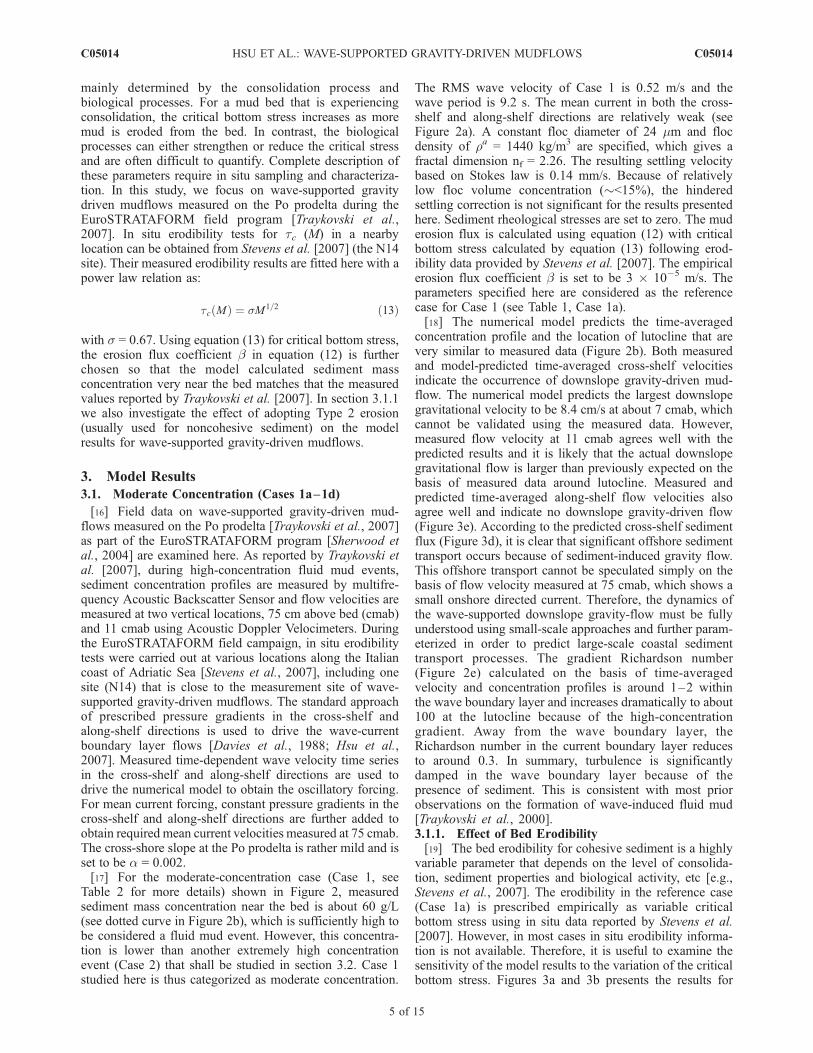
The RMS wave velocity of Case 1 is 0.52 m/s and thewave period is 9.2 s. The mean current in both the cross-shelf and along-shelf directions are relatively weak (seeFigure 2a). A constant floc diameter of 24 mm and flocdensity of ra = 1440 kg/m3 are specified, which gives afractal dimension nf = 2.26. The resulting settling velocitybased on Stokes law is 0.14 mm/s. Because of relativelylow floc volume concentration (�<15%), the hinderedsettling correction is not significant for the results presentedhere. Sediment rheological stresses are set to zero. The muderosion flux is calculated using equation (12) with criticalbottom stress calculated by equation (13) following erod-ibility data provided by Stevens et al. [2007]. The empiricalerosion flux coefficient b is set to be 3 � 10�5 m/s. Theparameters specified here are considered as the referencecase for Case 1 (see Table 1, Case 1a).[18] The numerical model predicts the time-averaged

concentration profile and the location of lutocline that arevery similar to measured data (Figure 2b). Both measuredand model-predicted time-averaged cross-shelf velocitiesindicate the occurrence of downslope gravity-driven mud-flow. The numerical model predicts the largest downslopegravitational velocity to be 8.4 cm/s at about 7 cmab, whichcannot be validated using the measured data. However,measured flow velocity at 11 cmab agrees well with thepredicted results and it is likely that the actual downslopegravitational flow is larger than previously expected on thebasis of measured data around lutocline. Measured andpredicted time-averaged along-shelf flow velocities alsoagree well and indicate no downslope gravity-driven flow(Figure 3e). According to the predicted cross-shelf sedimentflux (Figure 3d), it is clear that significant offshore sedimenttransport occurs because of sediment-induced gravity flow.This offshore transport cannot be speculated simply on thebasis of flow velocity measured at 75 cmab, which shows asmall onshore directed current. Therefore, the dynamics ofthe wave-supported downslope gravity-flow must be fullyunderstood using small-scale approaches and further param-eterized in order to predict large-scale coastal sedimenttransport processes. The gradient Richardson number(Figure 2e) calculated on the basis of time-averagedvelocity and concentration profiles is around 1–2 withinthe wave boundary layer and increases dramatically to about100 at the lutocline because of the high-concentrationgradient. Away from the wave boundary layer, theRichardson number in the current boundary layer reducesto around 0.3. In summary, turbulence is significantlydamped in the wave boundary layer because of thepresence of sediment. This is consistent with most priorobservations on the formation of wave-induced fluid mud[Traykovski et al., 2000].3.1.1. Effect of Bed Erodibility[19] The bed erodibility for cohesive sediment is a highly

variable parameter that depends on the level of consolida-tion, sediment properties and biological activity, etc [e.g.,Stevens et al., 2007]. The erodibility in the reference case(Case 1a) is prescribed empirically as variable criticalbottom stress using in situ data reported by Stevens et al.[2007]. However, in most cases in situ erodibility informa-tion is not available. Therefore, it is useful to examine thesensitivity of the model results to the variation of the criticalbottom stress. Figures 3a and 3b presents the results for


5 of 15

C05014

critical bottom stress and total eroded mass during thepassage of the wave group for Case 1a. Because of thesmall settling velocity, the total suspended sediment massdoes not respond to individual waves (compare Figure 3b

and Figure 2a). And in fact, the variation of total erodedmass and hence the critical bottom stress appears to evolvesomewhat with the envelope of the wave group. But we canconclude that their overall changes in magnitude are rather

Figure 2. Model-data comparison of wave-supported gravity-driven mudflow at Po prodelta formoderate-concentration conditions (Case 1a). (a) Measured 520-s wave-current velocities time series inthe cross-shelf (solid curve) and along-shelf (dashed curve) directions at 75 cmab [Traykovski et al.,2007] are used to drive the fluid mud model, (b) time-averaged mud concentration with the solid curverepresenting model results and dotted curve representing measured data, (c) modeled (solid curve) andmeasured (circles) time-averaged cross-shelf velocity profiles, (d) model results for cross-shelf sedimentflux, (e) model results for gradient Richardson number based on time-averaged concentration andvelocity profiles, (f) modeled (solid curve) and measured (crosses) time-averaged along-shelf velocityprofile, and (g) model results for along-shelf sediment flux.

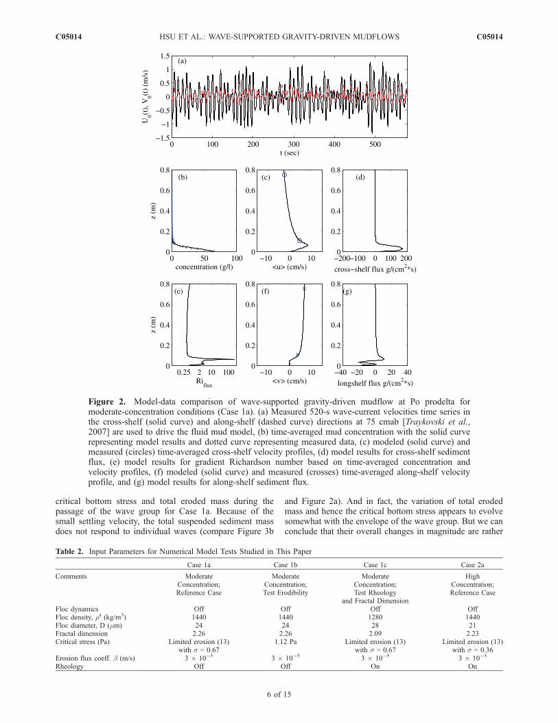
Table 2. Input Parameters for Numerical Model Tests Studied in This Paper

Case 1a Case 1b Case 1c Case 2a

Comments ModerateConcentration;Reference Case

ModerateConcentration;Test Erodibility

ModerateConcentration;Test Rheology

and Fractal Dimension

HighConcentration;Reference Case

Floc dynamics Off Off Off OffFloc density, ra (kg/m3) 1440 1440 1280 1440Floc diameter, D (mm) 24 24 28 21Fractal dimension 2.26 2.26 2.09 2.23Critical stress (Pa) Limited erosion (13)

with s = 0.671.12 Pa Limited erosion (13)

with s = 0.67Limited erosion (13)

with s = 0.36Erosion flux coeff. b (m/s) 3 � 10�5 3 � 10�5 3 � 10�5 3 � 10�5

Rheology Off Off On On


6 of 15

C05014

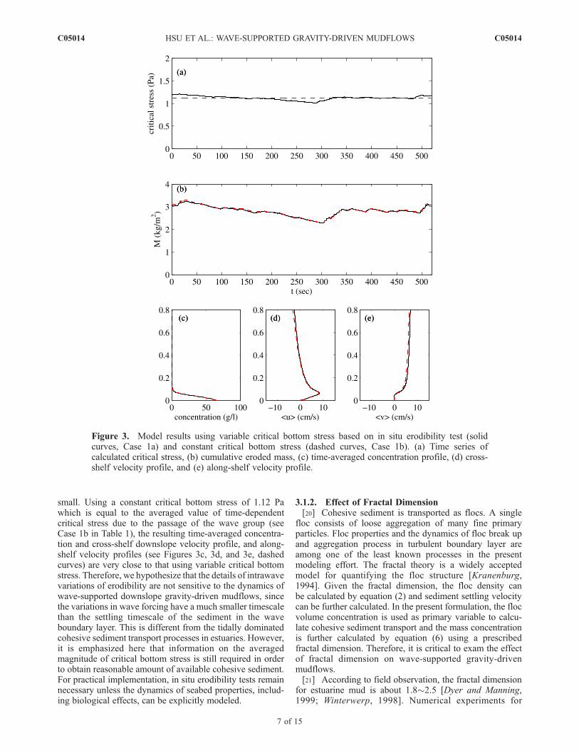
small. Using a constant critical bottom stress of 1.12 Pawhich is equal to the averaged value of time-dependentcritical stress due to the passage of the wave group (seeCase 1b in Table 1), the resulting time-averaged concentra-tion and cross-shelf downslope velocity profile, and along-shelf velocity profiles (see Figures 3c, 3d, and 3e, dashedcurves) are very close to that using variable critical bottomstress. Therefore, we hypothesize that the details of intrawavevariations of erodibility are not sensitive to the dynamics ofwave-supported downslope gravity-driven mudflows, sincethe variations in wave forcing have a much smaller timescalethan the settling timescale of the sediment in the waveboundary layer. This is different from the tidally dominatedcohesive sediment transport processes in estuaries. However,it is emphasized here that information on the averagedmagnitude of critical bottom stress is still required in orderto obtain reasonable amount of available cohesive sediment.For practical implementation, in situ erodibility tests remainnecessary unless the dynamics of seabed properties, includ-ing biological effects, can be explicitly modeled.

3.1.2. Effect of Fractal Dimension[20] Cohesive sediment is transported as flocs. A single

floc consists of loose aggregation of many fine primaryparticles. Floc properties and the dynamics of floc break upand aggregation process in turbulent boundary layer areamong one of the least known processes in the presentmodeling effort. The fractal theory is a widely acceptedmodel for quantifying the floc structure [Kranenburg,1994]. Given the fractal dimension, the floc density canbe calculated by equation (2) and sediment settling velocitycan be further calculated. In the present formulation, the flocvolume concentration is used as primary variable to calcu-late cohesive sediment transport and the mass concentrationis further calculated by equation (6) using a prescribedfractal dimension. Therefore, it is critical to exam the effectof fractal dimension on wave-supported gravity-drivenmudflows.[21] According to field observation, the fractal dimension

for estuarine mud is about 1.8�2.5 [Dyer and Manning,1999; Winterwerp, 1998]. Numerical experiments for

Figure 3. Model results using variable critical bottom stress based on in situ erodibility test (solidcurves, Case 1a) and constant critical bottom stress (dashed curves, Case 1b). (a) Time series ofcalculated critical stress, (b) cumulative eroded mass, (c) time-averaged concentration profile, (d) cross-shelf velocity profile, and (e) along-shelf velocity profile.


7 of 15

C05014

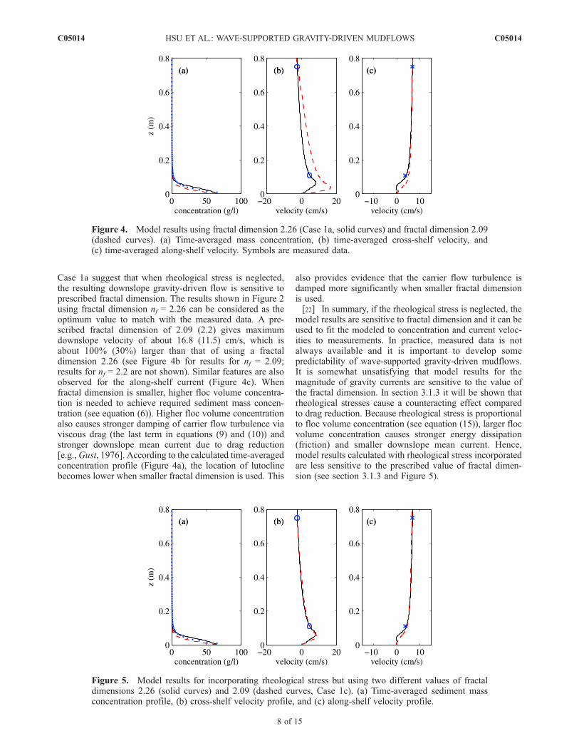
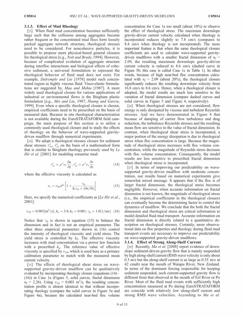
Case 1a suggest that when rheological stress is neglected,the resulting downslope gravity-driven flow is sensitive toprescribed fractal dimension. The results shown in Figure 2using fractal dimension nf = 2.26 can be considered as theoptimum value to match with the measured data. A pre-scribed fractal dimension of 2.09 (2.2) gives maximumdownslope velocity of about 16.8 (11.5) cm/s, which isabout 100% (30%) larger than that of using a fractaldimension 2.26 (see Figure 4b for results for nf = 2.09;results for nf = 2.2 are not shown). Similar features are alsoobserved for the along-shelf current (Figure 4c). Whenfractal dimension is smaller, higher floc volume concentra-tion is needed to achieve required sediment mass concen-tration (see equation (6)). Higher floc volume concentrationalso causes stronger damping of carrier flow turbulence viaviscous drag (the last term in equations (9) and (10)) andstronger downslope mean current due to drag reduction[e.g.,Gust, 1976]. According to the calculated time-averagedconcentration profile (Figure 4a), the location of lutoclinebecomes lower when smaller fractal dimension is used. This

also provides evidence that the carrier flow turbulence isdamped more significantly when smaller fractal dimensionis used.[22] In summary, if the rheological stress is neglected, the

model results are sensitive to fractal dimension and it can beused to fit the modeled to concentration and current veloc-ities to measurements. In practice, measured data is notalways available and it is important to develop somepredictability of wave-supported gravity-driven mudflows.It is somewhat unsatisfying that model results for themagnitude of gravity currents are sensitive to the value ofthe fractal dimension. In section 3.1.3 it will be shown thatrheological stresses cause a counteracting effect comparedto drag reduction. Because rheological stress is proportionalto floc volume concentration (see equation (15)), larger flocvolume concentration causes stronger energy dissipation(friction) and smaller downslope mean current. Hence,model results calculated with rheological stress incorporatedare less sensitive to the prescribed value of fractal dimen-sion (see section 3.1.3 and Figure 5).

Figure 4. Model results using fractal dimension 2.26 (Case 1a, solid curves) and fractal dimension 2.09(dashed curves). (a) Time-averaged mass concentration, (b) time-averaged cross-shelf velocity, and(c) time-averaged along-shelf velocity. Symbols are measured data.

Figure 5. Model results for incorporating rheological stress but using two different values of fractaldimensions 2.26 (solid curves) and 2.09 (dashed curves, Case 1c). (a) Time-averaged sediment massconcentration profile, (b) cross-shelf velocity profile, and (c) along-shelf velocity profile.


8 of 15

C05014

3.1.3. Effect of Mud Rheology[23] When fluid mud concentration becomes sufficiently

large such that the collisions among aggregates becomerather frequent or the concentrated mud flocs form looselypacked aggregate network structure, rheological stressesneed to be considered. For noncohesive particles, it ispossible to propose more physical-based general closuresfor rheological stress [e.g., Nott and Brady, 1994]. However,because of complicated evolution of aggregate structureduring interfloc interactions and biological effects of cohe-sive sediment, a universal formulation to represent therheological behavior of fluid mud does not exist. Forexample, Dalrymple and Liu [1978] model such concen-trated region as highly viscous fluid. Visco-elastic formula-tions are suggested by, Maa and Mehta [1987]. A morewidely used rheological closure for various applications ofindustrial or environmental flows is the Bingham plasticformulation [e.g., Mei and Liu, 1987; Huang and Garcia,1999]. Even when a specific rheological closure is chosen,empirical coefficients need to be prescribed on the basis ofmeasured data. Because in situ rheological characterizationis not available during the EuroSTRATAFORM field cam-paign, the main purpose of this section is to utilize acommonly used rheological closure and to study the effectsof rheology on the behavior of wave-supported gravity-driven mudflow through numerical experiments.[24] We adopt a rheological stresses closure for sediment

shear stresses txzs , tyz

s on the basis of a mathematical formthat is similar to Bingham rheology previously used by LeHir et al. [2001] for modeling estuarine mud:

tsxz ¼ r f ns@u

@z; tsyz ¼ r f ns

@v

@zð14Þ

where the effective viscosity is calculated as

ns ¼ ns0fka 1þ g0kbg0 þ @u=@zj j

ð15Þ

Here, we specify the numerical coefficients as [Le Hir et al.,2001]:

ns0 ¼ 0:003 m2=s� �

; ka ¼ 3:0; kb ¼ 0:001; g0 ¼ 1:0 1=secð Þ ð16Þ

Notice that g0 is shown in equation (15) to balance thedimension and in fact is not an empirical parameter. Theother three empirical parameters shown in (16) controlthe intensity of rheological viscosity and yield stress. Theyield stress is controlled by kb. The effective viscosityincreases with mud concentration via a power law functionwith a prescribed ka. The reference value of effectiveviscosity is specified by ns0, which is used here as a primarycalibration parameter to match with the measured meancurrent velocity.[25] The effects of rheological shear stress on wave-

supported gravity-driven mudflow can be qualitativelyevaluated by incorporating rheology closure (equations (14)–(16)) in Case 1a (Figure 5, solid curves, fractal dimensionnf = 2.26). Using ns0 = 0.003 m2/s, the resulting concen-tration profile is almost identical to that without incorpo-rating rheology (compare the solid curves in Figure 5a andFigure 4a), because the calculated near-bed floc volume

concentration for Case 1a too small (about 10%) to observethe effect of rheological stress. The maximum downslopegravity-driven current velocity calculated when rheology isincorporated reduces slightly to 7.8 cm/s (compares to8.4 cm/s when rheology is not incorporated). The moreimportant feature is that when the same rheological closurecoefficients are used to calculate wave-supported gravity-driven mudflows with a smaller fractal dimension of nf =2.09, the resulting maximum downslope gravity-drivencurrent velocity is reduced to 8.6 cm/s (dashed curve inFigure 5b; this case is called Case 1c in Table 1). In otherwords, because of high near-bed floc concentration calcu-lated with nf = 2.09 (about 20%), the rheological closuresignificantly reduces the resulting downslope velocity from16.8 cm/s to 8.6 cm/s. Hence, when a rheological closure isadopted, the model results are much less sensitive to thevariation of fractal dimension (compare dashed curves andsolid curves in Figure 5 and Figure 4, respectively).[26] When rheological stresses are not considered, flow

energy is only dissipated by viscous and turbulent Reynoldsstresses. And we have demonstrated in Figure 4 thatbecause of damping of carrier flow turbulence and dragreduction, the turbulence Reynolds stresses and the resultingmean flow are sensitive to the value of fractal dimension. Incontrast, when rheological shear stress is incorporated, amajor portion of the energy dissipation is due to rheologicalstress when floc concentration is large. Because the magni-tude of rheological stress increases with floc volume con-centration, while the magnitude of Reynolds stress decreasewith floc volume concentration. Consequently, the modelresults are less sensitive to prescribed fractal dimensionwhen rheological stress is incorporated.[27] In terms of improving our predictability on wave-

supported gravity-driven mudflow with moderate concen-tration, our results based on numerical experiments givesomewhat mixed message. It appears that if the floc is oflarger fractal dimension, the rheological stress becomesnegligible. However, when accurate information on fractaldimension is not known, the magnitude of rheological stress(i.e., the empirical coefficients in the rheological closure)can eventually become the determining factor to control thedynamics of mudflow. We conclude that the both the fractaldimension and rheological stress are critical information tomodel detailed fluid mud transport. Accurate information onfractal dimension is directly related to a quantitative de-scription on rheological stresses. Certainly, more observa-tional data on floc properties and rheology during fluid mudtransport events are necessary to improve our predictabilityon wave-supported gravity-driven mudflows.3.1.4. Effect of Strong Along-Shelf Current[28] Recently, Ma et al. [2008] report evidence of down-

slope sediment-driven gravity flow that is mainly suspendedby high along-shelf current (RMSwave velocity is only about0.3 m/s but the along-shelf current is as large as 0.35 m/s at42 cmab) near the mouth of Waiapu River, New Zealand.In terms of the dominant forcing responsible for keepingsediment suspended, such current-supported gravity flow isdifferent from that observed at the mouth of Eel River or PoRiver. Most of the fluid mud events with sufficiently highconcentration measured at Po during EuroSTRATAFORMare coincide with relatively low along-shelf current andstrong RMS wave velocities. According to Ma et al.


9 of 15

C05014

[2008], there are some characteristics of current-supportedgravity-driven sediment flow that are distinct from wave-supported ones. In current-supported condition, sediment isnot confined in the wave boundary layer because of strongcurrent-induced mixing and the magnitude of the resultingdownslope gravity flow is also larger.[29] The fluid mud model developed in this study is based

on a general wave-current bottom boundary layer formula-tion. Hence, the present model is utilized here to study theeffect of strong along-shelf current on wave-supportedgravity-driven mudflows by specifying a larger along-shelfpressure gradient in Case 1a. As shown in Figure 6e, largeralong-shelf pressure gradient causes stronger along-shelfcurrent of 30 cm/s at 80 cmab (solid curve), which is about4.5 times larger than that of Case 1a (dashed curve).Sediment is mixing is increased in the water column. Hence,the lutocline is located at around 25 cmab, which is about2�3 times higher than that of Case 1a (see Figure 6a).Moreover, the resulting downslope gravity-driven flowexceeds 20 cm/s (Figure 6b) and significant offshore andalong-shelf sediment transports are predicted (Figures 6cand 6f). These features are qualitatively consistent with fieldobserved features of current-supported gravity-driven flowat the mouth of Waiapu River, New Zealand [Ma et al.,2008]. More detailed model-data comparison and numericalmodeling study are necessary in order to better understandthe mechanisms and the parameterization of current-supported gravity-driven sediment flow.

3.2. High Concentration (Case 2)

[30] The near-bed fluid mud mass concentration observedin Case 2 exceeds 150 g/L (Figure 7a), which is more than

two times larger than the moderate-concentration case(Case 1 in section 3.1). However, measured RMS wavevelocity and wave period are 0.51 m/s and 8.9 s, respec-tively, which are similar to that of Case 1. Hence, it is likelythat Case 2 is observed when more soft mud is availableand the erodibility is larger to attain the observed highconcentration under similar wave intensity. According toTraykovski et al. [2007], Case 2 was measured at thebeginning of a wave event right after high–river dischargeevent [Traykovski et al., 2007, Figure 11, day 6.1]. Incontrast, Case 1 is measured about 4 h later after 50% to70% [see also Traykovski et al., 2007, Figure 11] of theavailable sediment had already been transported offshoreby the downslope gravity flows. Using a similar flocdiameter and fractal dimension that are used in Case 1a(ra = 1440 kg/m3 and D = 21 mm, nf = 2.23), the criticalbottom stress (see equation (13)) suggested by Stevens et al.[2007] is too large to achieve measured magnitude of mudmass concentration. To simulate more unconsolidated softmud during this high-concentration event, the critical bot-tom stress is reduced by setting s = 0.36 in equation (13).Model results further indicate that if rheology is notconsidered, the calculated downslope gravity-driven flowvelocity is several times larger than the observed data. Asexplained in sections 3.1.2 and 3.1.3, the calculated largedownslope current velocity is due to drag reduction phe-nomenon caused by damped turbulence via sediment den-sity stratification. Under such high mud concentration therheological stress is expected to be large. When Binghamrheology shown in equations (14)–(16) is incorporated(withns0 increased to 0.03 m2/s), the predicted downslope

Figure 6. Model results for wave-supported gravity-driven mudflows when strong along-shelf currentis applied to Case 1a (solid curves). Dashed curves represent results of Case 1a shown here for thepurpose of comparison. (a) Time-averaged mud concentration, (b) time-averaged cross-shelf velocityprofile, (c) cross-shelf sediment flux, model results for gradient Richardson number based on (d) time-averaged concentration and (e) velocity profiles, (f) time-averaged along-shelf velocity profile, and (g)along-shelf sediment flux.


10 of 15

C05014

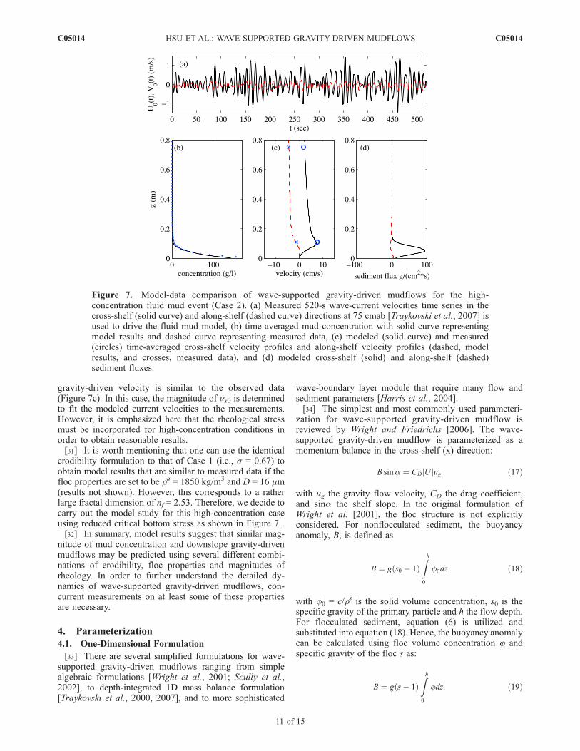
gravity-driven velocity is similar to the observed data(Figure 7c). In this case, the magnitude of ns0 is determinedto fit the modeled current velocities to the measurements.However, it is emphasized here that the rheological stressmust be incorporated for high-concentration conditions inorder to obtain reasonable results.[31] It is worth mentioning that one can use the identical

erodibility formulation to that of Case 1 (i.e., s = 0.67) toobtain model results that are similar to measured data if thefloc properties are set to be ra = 1850 kg/m3 and D = 16 mm(results not shown). However, this corresponds to a ratherlarge fractal dimension of nf = 2.53. Therefore, we decide tocarry out the model study for this high-concentration caseusing reduced critical bottom stress as shown in Figure 7.[32] In summary, model results suggest that similar mag-

nitude of mud concentration and downslope gravity-drivenmudflows may be predicted using several different combi-nations of erodibility, floc properties and magnitudes ofrheology. In order to further understand the detailed dy-namics of wave-supported gravity-driven mudflows, con-current measurements on at least some of these propertiesare necessary.

4. Parameterization

4.1. One-Dimensional Formulation

[33] There are several simplified formulations for wave-supported gravity-driven mudflows ranging from simplealgebraic formulations [Wright et al., 2001; Scully et al.,2002], to depth-integrated 1D mass balance formulation[Traykovski et al., 2000, 2007], and to more sophisticated

wave-boundary layer module that require many flow andsediment parameters [Harris et al., 2004].[34] The simplest and most commonly used parameteri-

zation for wave-supported gravity-driven mudflow isreviewed by Wright and Friedrichs [2006]. The wave-supported gravity-driven mudflow is parameterized as amomentum balance in the cross-shelf (x) direction:

B sina ¼ CD Uj jug ð17Þ

with ug the gravity flow velocity, CD the drag coefficient,and sina the shelf slope. In the original formulation ofWright et al. [2001], the floc structure is not explicitlyconsidered. For nonflocculated sediment, the buoyancyanomaly, B, is defined as

B ¼ g s0 � 1ð ÞZh0

f0dz ð18Þ

with f0 = c/rs is the solid volume concentration, s0 is thespecific gravity of the primary particle and h the flow depth.For flocculated sediment, equation (6) is utilized andsubstituted into equation (18). Hence, the buoyancy anomalycan be calculated using floc volume concentration 8 andspecific gravity of the floc s as:

B ¼ g s� 1ð ÞZh0

fdz: ð19Þ

Figure 7. Model-data comparison of wave-supported gravity-driven mudflows for the high-concentration fluid mud event (Case 2). (a) Measured 520-s wave-current velocities time series in thecross-shelf (solid curve) and along-shelf (dashed curve) directions at 75 cmab [Traykovski et al., 2007] isused to drive the fluid mud model, (b) time-averaged mud concentration with solid curve representingmodel results and dashed curve representing measured data, (c) modeled (solid curve) and measured(circles) time-averaged cross-shelf velocity profiles and along-shelf velocity profiles (dashed, modelresults, and crosses, measured data), and (d) modeled cross-shelf (solid) and along-shelf (dashed)sediment fluxes.


11 of 15

C05014

The total velocity in equation (17) is defined as

Uj j ¼ffiffiffiffiffiffiffiffiffiffiffiffiffiffiffiffiffiffiffiffiffiffiffiffiffiffiffiffiffiffiffiffiffiffiffiffiffiffiffiffiffiffiffiffiffiffiu2w þ v2w þ u2c þ v2c þ u2g

qð20Þ

with uw, uc and vw, vc the cross-shelf and along-shelf RMSwave velocity and mean current velocities, respectively.[35] This formulation is efficient to calculate large-scale

coastal sediment transport. However, it requires prioriknowledge on CD and B. On the basis of field data, CD iscalibrated to be around 0.001–0.004 [Wright et al., 2001;Traykovski et al., 2007]. The buoyancy anomaly is estimatedfrom the bulk Richardson number and total velocity [Wrightet al., 2001]:

B ¼ RiBU2 ð21Þ

[36] The bulk Richardson number of the fluid mud layeris often assumed to be 0.25, i.e., the critical Richardsonnumber with a marginally turbulent condition [e.g.,Trowbridge and Kineke, 1994]. Essentially, the total amountof suspended mud, phrased as buoyancy anomaly, is con-sidered as only a function of total velocity and an equilib-rium assumption is utilized such that the total amount ofsuspended sediment exactly matches the carrying capacityof the turbulent flow. However, according to Case 1 andCase 2 discussed in section 3.1 and 3.2, the total amount ofsuspended sediment is not always related to RMS wavevelocity but may be controlled by the availability of theunconsolidated mud. In addition, the critical Richardsonnumber concept is mostly applicable to steady or tidalboundary layers. Recent laboratory experiments and fieldmeasurements suggest that the bulk Richardson numberin the wave boundary layer is smaller than 0.25 [Lamband Parsons, 2005; Traykovski et al., 2007]. Hence, it

is necessary to further study the parameterization ofbuoyancy anomaly.[37] In summary, there are several key questions related

to the parameterization of wave-supported gravity-drivenmudflows that can be studied using the present numericalmodel: (1) What is the magnitude of CD and its dependenceon wave condition, the availability of mud and floc prop-erties? (2) What is the magnitude of bulk Richardsonnumber for wave-induced fluid mud layer and its depen-dence on wave condition, the availability of mud and flocproperties?[38] Detailed numerical model results allow us to evaluate

the parameters used in the aforementioned 1D formulation.The RMS wave velocities and mean current velocities in thecross-shelf and along-shelf directions are directly evaluatedfrom the time series measured at 75 cmab. The downslopegravity flow velocity ug is extracted from the model resultsbased on the maximum velocity observed near the bed.The buoyancy anomaly is obtained by numerical integra-tion of concentration across the water column according toequation (19). With all these physical quantities obtainedfrom the numerical model results, CD and RiB can becalculated using equations (17) and (21).

4.2. Effects of Wave Intensity and Erodibility

[39] The wave-supported gravity-driven mudflow studiedhere is different from the autosuspension turbidity current[Mulder and Syvitski, 1995; Imran and Syvitski, 2000]. Thesediment-induced gravity current considered here must besupported by ambient waves or currents. Hence it isimportant to study the effects of wave intensity on fluidmud transport. As also discussed previously, the RMS wavevelocities for moderate-concentration (Case 1) and high-concentration (Case 2) cases are similar. The major reasonthat is responsible for the observed large differences in fluidmud concentration appears to be erodibility. Using Case 1ashown in Figure 2 for moderate concentration and Case 2shown in Figure 8 for high concentration, further numericalexperiments are conducted by driving the model withseveral different intensities of wave velocity (see Tables 3and 4 for details).[40] For moderate-concentration condition (crosses in

Figure 8a), the magnitude of drag coefficient decays asRMS wave velocity increases, which is qualitatively similarto the logarithmic formula used by Harris et al. [2004].However, for high-concentration conditions (circles in Fig-ure 8) with rheological stress incorporated, the resultingmagnitude of drag coefficient is about 0.0013 and is more orless insensitive to the variations in wave intensity. Erodibil-ity can change the degree of dependence of drag coefficientson wave intensity. For highly erodible mud, small waves

Figure 8. (a) Drag coefficients (CD) versus RMS wavevelocity and (b) bulk Richardson number versus RMS wavevelocity for moderate-concentration conditions (crosses) andhigh-concentration conditions (circles). Detailed numericvalues are presented in Tables 3 and 4.

Table 3. Model Results for Different Magnitude of Wave Intensity

for Moderate-Concentration Condition

RMS WaveVelocity (m/s) jUj (m/s) ug (m/s) B (m2/s2) Cd RiB

0.26 0.281 0.014 0.0078 0.00397 0.098780.39 0.404 0.056 0.0141 0.00124 0.086340.52 0.531 0.084 0.0181 0.00081 0.064190.65 0.662 0.114 0.019 0.00050 0.043360.78 0.803 0.172 0.0166 0.00024 0.02574


12 of 15

C05014

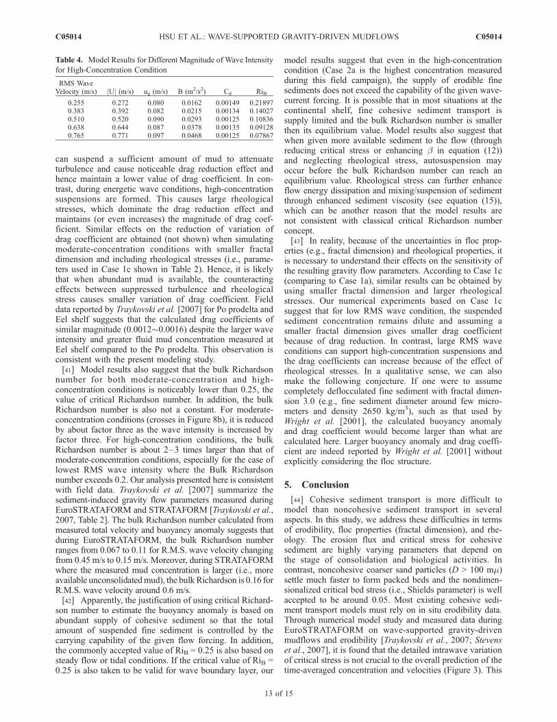
can suspend a sufficient amount of mud to attenuateturbulence and cause noticeable drag reduction effect andhence maintain a lower value of drag coefficient. In con-trast, during energetic wave conditions, high-concentrationsuspensions are formed. This causes large rheologicalstresses, which dominate the drag reduction effect andmaintains (or even increases) the magnitude of drag coef-ficient. Similar effects on the reduction of variation ofdrag coefficient are obtained (not shown) when simulatingmoderate-concentration conditions with smaller fractaldimension and including rheological stresses (i.e., parame-ters used in Case 1c shown in Table 2). Hence, it is likelythat when abundant mud is available, the counteractingeffects between suppressed turbulence and rheologicalstress causes smaller variation of drag coefficient. Fielddata reported by Traykovski et al. [2007] for Po prodelta andEel shelf suggests that the calculated drag coefficients ofsimilar magnitude (0.0012�0.0016) despite the larger waveintensity and greater fluid mud concentration measured atEel shelf compared to the Po prodelta. This observation isconsistent with the present modeling study.[41] Model results also suggest that the bulk Richardson

number for both moderate-concentration and high-concentration conditions is noticeably lower than 0.25, thevalue of critical Richardson number. In addition, the bulkRichardson number is also not a constant. For moderate-concentration conditions (crosses in Figure 8b), it is reducedby about factor three as the wave intensity is increased byfactor three. For high-concentration conditions, the bulkRichardson number is about 2–3 times larger than that ofmoderate-concentration conditions, especially for the case oflowest RMS wave intensity where the Bulk Richardsonnumber exceeds 0.2. Our analysis presented here is consistentwith field data. Traykovski et al. [2007] summarize thesediment-induced gravity flow parameters measured duringEuroSTRATAFORM and STRATAFORM [Traykovski et al.,2007, Table 2]. The bulk Richardson number calculated frommeasured total velocity and buoyancy anomaly suggests thatduring EuroSTRATAFORM, the bulk Richardson numberranges from 0.067 to 0.11 for R.M.S. wave velocity changingfrom 0.45 m/s to 0.15 m/s. Moreover, during STRATAFORMwhere the measured mud concentration is larger (i.e., moreavailable unconsolidatedmud), the bulk Richardson is 0.16 forR.M.S. wave velocity around 0.6 m/s.[42] Apparently, the justification of using critical Richard-

son number to estimate the buoyancy anomaly is based onabundant supply of cohesive sediment so that the totalamount of suspended fine sediment is controlled by thecarrying capability of the given flow forcing. In addition,the commonly accepted value of RiB = 0.25 is also based onsteady flow or tidal conditions. If the critical value of RiB =0.25 is also taken to be valid for wave boundary layer, our

model results suggest that even in the high-concentrationcondition (Case 2a is the highest concentration measuredduring this field campaign), the supply of erodible finesediments does not exceed the capability of the given wave-current forcing. It is possible that in most situations at thecontinental shelf, fine cohesive sediment transport issupply limited and the bulk Richardson number is smallerthen its equilibrium value. Model results also suggest thatwhen given more available sediment to the flow (throughreducing critical stress or enhancing b in equation (12))and neglecting rheological stress, autosuspension mayoccur before the bulk Richardson number can reach anequilibrium value. Rheological stress can further enhanceflow energy dissipation and mixing/suspension of sedimentthrough enhanced sediment viscosity (see equation (15)),which can be another reason that the model results arenot consistent with classical critical Richardson numberconcept.[43] In reality, because of the uncertainties in floc prop-

erties (e.g., fractal dimension) and rheological properties, itis necessary to understand their effects on the sensitivity ofthe resulting gravity flow parameters. According to Case 1c(comparing to Case 1a), similar results can be obtained byusing smaller fractal dimension and larger rheologicalstresses. Our numerical experiments based on Case 1csuggest that for low RMS wave condition, the suspendedsediment concentration remains dilute and assuming asmaller fractal dimension gives smaller drag coefficientbecause of drag reduction. In contrast, large RMS waveconditions can support high-concentration suspensions andthe drag coefficients can increase because of the effect ofrheological stresses. In a qualitative sense, we can alsomake the following conjecture. If one were to assumecompletely deflocculated fine sediment with fractal dimen-sion 3.0 (e.g., fine sediment diameter around few micro-meters and density 2650 kg/m3), such as that used byWright et al. [2001], the calculated buoyancy anomalyand drag coefficient would become larger than what arecalculated here. Larger buoyancy anomaly and drag coeffi-cient are indeed reported by Wright et al. [2001] withoutexplicitly considering the floc structure.

5. Conclusion

[44] Cohesive sediment transport is more difficult tomodel than noncohesive sediment transport in severalaspects. In this study, we address these difficulties in termsof erodibility, floc properties (fractal dimension), and rhe-ology. The erosion flux and critical stress for cohesivesediment are highly varying parameters that depend onthe stage of consolidation and biological activities. Incontrast, noncohesive coarser sand particles (D > 100 mm)settle much faster to form packed beds and the nondimen-sionalized critical bed stress (i.e., Shields parameter) is wellaccepted to be around 0.05. Most existing cohesive sedi-ment transport models must rely on in situ erodibility data.Through numerical model study and measured data duringEuroSTRATAFORM on wave-supported gravity-drivenmudflows and erodibility [Traykovski et al., 2007; Stevenset al., 2007], it is found that the detailed intrawave variationof critical stress is not crucial to the overall prediction of thetime-averaged concentration and velocities (Figure 3). This

Table 4. Model Results for Different Magnitude of Wave Intensity

for High-Concentration Condition

RMS WaveVelocity (m/s) jUj (m/s) ug (m/s) B (m2/s2) Cd RiB

0.255 0.272 0.080 0.0162 0.00149 0.218970.383 0.392 0.082 0.0215 0.00134 0.140270.510 0.520 0.090 0.0293 0.00125 0.108360.638 0.644 0.087 0.0378 0.00135 0.091280.765 0.771 0.097 0.0468 0.00125 0.07867


13 of 15

C05014

is because the settling timescale (i.e., wave boundary layerthickness divided by settling velocity, which is around10 min) is in general much larger than intrawave period(�10 s). However, in situ information on near-bed concen-tration or averaged erodibility is still necessary to match thetotal amount of suspended fluid mud. The consolidationtimescale (hours and days) is also much larger than theintrawave and settling timescales considered here, suggestingthat a stand alone consolidation module [Sanford, 2008]may be incorporated in the cohesive sediment transportmodel to provide bulk averaged erodibility information. Amore challenging situation that deserves more future studyis when wave forcing is actively fluidizing the mud bed andincreasing the erodibility.[45] Unlike noncohesive sediments, cohesive sediment is

transported as floc aggregates, which present additionalunknowns in floc properties and the changes of floc size(floc dynamics) in the carrier flow [e.g., Winterwerp, 1998;Son and Hsu, 2008]. The basic mud floc properties aredetermined by the fractal dimension, which is qualitativelyagreed upon to be around 2 but its specific value cannot bedetermined without in situ data. Model results suggest thatwhen rheological stresses are not incorporated (or negligi-ble), the predicted cross-shelf and along-shelf currents aresensitive to the prescribed fractal dimension. Smaller fractaldimension requires larger floc volume concentration tomatch the measured fluid mud mass concentration, whichgives larger mean current velocity because of dampedturbulence via drag reduction. The rheological closure forcohesive sediment is another highly empirical component.The role of rheological stress is to cause more friction(energy dissipation via interfloc interactions) in the bound-ary layer and hence incorporating larger rheological stressesreduces mean current. Our numerical study implies twoscenarios that may occur in reality: For relatively lowconcentration fluid mud suspension (�10 g/L) with negli-gible rheological stresses, floc properties defined by thefractal dimension is the most important physical quantitythat controls the dynamics of wave-supported gravity-driven mudflows. For high-concentration fluid mud suspen-sions (10 g/L) with rheological stresses dominatingturbulent Reynolds stress in the fluid mud layer, uncertain-ties in fractal dimension are of less importance, and thedynamics of fluid mud transport are controlled by therheological closure. It is extremely desirable for the researchcommunity to further investigate floc properties and rheo-logical stress during cohesive sediment transport through insitu measurements and more detailed modeling.[46] Despite this study’s focus on wave-supported gravity-

driven mudflows, the numerical model developed here isbased on general wave-current boundary layer formulationand is also able to model current-supported downslopegravity-driven mudflows. Through numerical experimentwe demonstrate that the present model predicts current-driven sediment-induced gravity flow characteristics thatare consistent with recently observed field data at the mouthof Waiapu River, New Zealand [Ma et al., 2008].[47] By analyzing the results of many numerical model

experiments, gravity flow parameters used in the 1D pa-rameterization [Wright et al., 2001] are discussed. When theavailability of mud is abundant, the counteracting effectsbetween attenuated turbulence and rheological stress allow a

more or less constant value of drag coefficient for differentwave intensity, consistent with prior field observations. Thecalculated bulk Richardson number is smaller than thecritical Richardson number 0.25, suggesting a supply lim-ited condition for unconsolidated mud and/or a distinctdifference between tidal and wave boundary layer processes.Moreover, the resulting bulk Richardson number and dragcoefficient are also sensitive to prescribed floc properties andrheological stresses. In order to provide more accurateparameterization of wave-supported gravity-driven mud-flows for large-scale coastal models, in situ erodibility andfloc structure characterizations are critical.

[48] Acknowledgments. This study is supported by the Office ofNaval Research grant N00014-09-1-0134 and grant N00014-06-1-0945 aspart of the Community Sediment Transport Modeling System (CSTMS)through the National Oceanographic Partnership Program (NOPP). Thisstudy is also partially supported by National Science Foundation (OCE-0644497).

ReferencesAllen, J. R. L. (1985), Principles of Physical Sedimentology, Allen andUnwin, London.

Dadson, S., N. Hovius, S. Pegg, W. B. Dade, M. J. Horng, and H. Chen(2005), Hyperpycnal river flows from an active mountain belt, J. Geo-phys. Res., 110, F04016, doi:10.1029/2004JF000244.

Dalrymple, R. A., and P. L. Liu (1978), Waves over soft mud beds: A two-layer fluid mud model, J. Phys. Oceanogr., 8, 1121–1131, doi:10.1175/1520-0485(1978)008<1121:WOSMAT>2.0.CO;2.

Davies, A. G., R. L. Soulsby, and H. L. King (1988), A numerical model ofthe combined wave and current bottom boundary layer, J. Geophys. Res.,93, 491–508, doi:10.1029/JC093iC01p00491.

Dyer, K. R., and A. J. Manning (1999), Observation of the size, settlingvelocity and effective density of flocs, and their fractal dimensions, J. SeaRes., 41, 87–95, doi:10.1016/S1385-1101(98)00036-7.

Fan, S., D. J. P. Swift, P. A. Traykovski, S. J. Bentley, J. C. Borgeld, C. W.Reed, and A. W. Niedoroda (2004), River flooding, storm resuspension,and event stratigraphy on the northern California shelf: Observationscompared with simulations, Mar. Geol., 210, 17–41, doi:10.1016/j.margeo.2004.05.024.

Ferry, J., and S. Balachandar (2001), A fast Eulerian method for dispersetwo-phase flow, Int. J. Multiphase Flow, 27, 1199–1226, doi:10.1016/S0301-9322(00)00069-0.

Friedrichs, C. T., and L. D. Wright (2004), Gravity-driven sediment trans-port on the continental shelf: Implications for equilibrium profiles nearriver mouth, Coastal Eng., 51, 795 –811, doi:10.1016/j.coastaleng.2004.07.010.

Geyer, W. R., P. Hill, T. Milligan, and P. Traykovski (2000), The structureof the Eel River plume during floods, Cont. Shelf Res., 20, 2067–2093,doi:10.1016/S0278-4343(00)00063-7.

Gust, G. (1976), Observations on turbulent-drag reduction in a dilute sus-pension of clay in sea-water, J. Fluid Mech., 75, 29–47, doi:10.1017/S0022112076000116.

Harris, C. K., P. A. Traykovski, and R. W. Geyer (2004), Including a near-bed turbid layer in a three-dimensional sediment transport model withapplication to the Eel River shelf, northern California, in Proceedings ofthe Eighth Conference on Estuarine and Coastal Modeling, edited byM. Spaulding, pp. 784–803, Am. Soc. of Civ. Eng., Reston, Va.

Harris, C. K., P. A. Traykovski, and W. R. Geyer (2005), Flood dispersaland deposition by near-bed gravitational sediment flows and oceano-graphic transport: A numerical modeling study of the Eel River shelf,northern California, J. Geophys. Res., 110, C09025, doi:10.1029/2004JC002727.

Hsu, T.-J., P. A. Traykovski, and G. C. Kineke (2007), On modeling bound-ary layer and gravity-driven fluid mud transport, J. Geophys. Res., 112,C04011, doi:10.1029/2006JC003719.

Huang, X., and M. H. Garcia (1999), Modeling of non-hydroplaning mud-flows on continental slopes, Mar. Geol., 154, 131–142, doi:10.1016/S0025-3227(98)00108-X.

Imran, J., and J. P. M. Syvitski (2000), Impact of extreme river events onthe coastal ocean, Oceanography, 13, 85–92.

Kranenburg, C. (1994), The fractal structure of cohesive sediment aggre-gates, Estuarine Coastal Shelf Sci., 39, 451–460.

Lamb, M. P., and J. D. Parsons (2005), High-density suspensions formedunder waves, J. Sediment. Res., 75, 386–397, doi:10.2110/jsr.2005.030.


14 of 15

C05014

Le Hir, P., P. Bassoulet, and H. Jestin (2001), Application of the continuousmodeling concept to simulate high-concentration suspended sediment ina macro-tidal estuary, in Coastal and Estuarine Fine Sediment Processes,Proc. Mar. Sci., vol. 3, edited by W. H. McAnally and A. J. Metha,pp. 229–248, Elsevier Sci., Amsterdam.

Lesser, G. R., J. A. Roelvink, A. T. M. J.van Kester, and G. S. Stelling(2004), Development of a three-dimensional morphological model,Coastal Eng., 51, 883–915, doi:10.1016/j.coastaleng.2004.07.014.

Ma, Y., D. L. Wright, and C. F. Friedrichs (2008), Observation of sedimenttransport on the continental shelf off the mouth of the Waiapu River, NewZealand: Evidence for current-supported gravity flows, Cont. Shelf Res.,28, 516–532, doi:10.1016/j.csr.2007.11.001.

Maa, P.-Y., and A. J. Mehta (1987), Mud erosion by waves: A laboratorystudy, Cont. Shelf Res., 7, 1269–1284.

Mei, C. C., and K. F. Liu (1987), A Bingham plastic model for a muddyseabed under long waves, J. Geophys. Res., 92, 14,581 – 14,594,doi:10.1029/JC092iC13p14581.

Milliman, J. D., and S. J. Kao (2005), Hyperpycnal discharge of fluvialsediment to the ocean: Impact of Super-Typhoon Herb (1996) on Taiwa-nese rivers, J. Geol., 113, 503–506, doi:10.1086/431906.

Milliman, J. D., and J. P. M. Syvitski (1992), Geomorphic/tectonic controlof sediment discharge to the ocean: The importance of small mountainrivers, J. Geol., 100, 525–544.

Milliman, J. D., S. W. Lin, S. J. Kao, J. P. Liu, C. S. Liu, J. K. Chiu, andY. C. Lin (2007), Short-term changes in seafloor character due to flood-derived hyperpycnal discharge: Typhoon Mindulle, Taiwan, July 2004,Geology, 35, 779–782, doi:10.1130/G23760A.1.

Mulder, T., and J. P. M. Syvitski (1995), Turbidity currents generated atriver mouths during exceptional discharges to the world oceans, J. Geol.,103, 285–299.

Nittrouer, C. A., and J. H. Kravitz (1996), STRATAFORM: A program tostudy the creation and interpretation of sedimentary strata on continentalmargins, Oceanography, 9, 146–152.

Nott, P. R., and J. F. Brady (1994), Pressure-driven flow of suspension:Simulation and theory, J. Fluid Mech., 275, 157–199, doi:10.1017/S0022112094002326.

Ogston, A. S., D. A. Cacchione, R. W. Sternberg, and C. G. Kineke (2000),Observation of storm and river flood-driven sediment transport on thenorthern California continental shelf, Cont. Shelf Res., 20, 2141–2162,doi:10.1016/S0278-4343(00)00065-0.

Parker, G. (1982), Condition for the ignition of catastrophically erosiveturbidity currents, Mar. Geol., 46, 307 – 327, doi:10.1016/0025-3227(82)90086-X.

Richardson, J. F., and W. N. Zaki (1954), Sedimentation and fluidization,part 1, Trans. Inst. Chem. Eng., 32, 35–53.

Sanford, L. P. (2008), Modeling a dynamically varying mixed sedimentbed with erosion, deposition, bioturbation, consolidation, and armoring,Comput. Geosci., 34, 1263–1283, doi:10.1016/j.cageo.2008.02.011.

Sanford, L. P., and J. P. Halka (1993), Assessing the paradigm of mutuallyexclusive erosion and deposition of mud, with examples from upperChesapeake Bay, Mar. Geol., 114, 37 – 57, doi:10.1016/0025-3227(93)90038-W.

Sanford, L. P., and J. P.-Y. Maa (2001), A unified erosion formulationfor fine sediments, Mar. Geol., 179, 9 –23, doi:10.1016/S0025-3227(01)00201-8.

Scully, M. E., C. T. Friedrichs, and L. D. Wright (2002), Application of ananalytical model of critically stratified gravity-driven sediment transportand deposition to observations from the Eel River continental shelf,northern California, Cont. Shelf Res., 22, 1951–1974, doi:10.1016/S0278-4343(02)00047-X.

Sherwood, C. R., et al. (2004), Sediment dynamics in the Adriatic Seainvestigated with coupled models, Oceanography, 17, 58–69.

Son, M., and T.-J. Hsu (2008), Flocculation model of cohesive sedimentusing variable fractal dimension, Environ. Fluid Mech., 8, 55 – 71,doi:10.1007/s10652-007-9050-7.

Stevens, A. W., R. A. Wheatcroft, and P. L. Wiberg (2007), Seabed proper-ties and sediment erodibility along the western Adriatic margin, Italy,Cont. Shelf Res., 27, 400–416, doi:10.1016/j.csr.2005.09.009.

Syvitski, J. P. M., J. N. Smith, E. A. Calabrese, and B. P. Boudreau (1988),Basin sedimentation and the growth of prograding deltas, J. Geophys.Res., 93, 6895–6908, doi:10.1029/JC093iC06p06895.

Traykovski, P., W. R. Geyer, J. D. Irish, and J. F. Lynch (2000), The role ofwave-induced fluid mud flows for cross-shelf transport on the Eel Rivercontinental shelf, Cont. Shelf Res., 20, 2113–2140, doi:10.1016/S0278-4343(00)00071-6.

Traykovski, P., P. Wiberg, and W. R. Geyer (2007), Observations andmodeling of wave-supported sediment gravity flows on the Po prodeltaand comparison to prior observations from the Eel shelf, Cont. Shelf Res.,27, 375–399, doi:10.1016/j.csr.2005.07.008.

Trowbridge, J. H., and G. C. Kineke (1994), Structure and dynamics offluid mud on the Amazon continental shelf, J. Geophys. Res., 99, 865–874, doi:10.1029/93JC02860.

van der Ham, R., and J. C. Winterwerp (2001), Turbulent exchange of finesediments in a tidal channel in the Ems/Dollard estuary. Part I: Analysiswith a 1DV numerical model, Cont. Shelf Res., 21, 1629 – 1647,doi:10.1016/S0278-4343(01)00011-5.

Vinzon, S. B., and A. J. Mehta (1998), Mechanism for formation of luto-clines by waves, J. Waterw. Port Coastal Ocean Eng., 124, 147–149,doi:10.1061/(ASCE)0733-950X(1998)124:3(147).

Warner, J. C., C. R. Sherwood, R. P. Signell, C. K. Harris, and H. G.Arango (2008), Development of a three-dimensional, regional, coupledwave, current and sediment-transport model, Comput. Geosci., 34,1284–1306, doi:10.1016/j.cageo.2008.02.012.

Wheatcroft, R. A. (2000), Oceanic flood sedimentation: A new perspective,Cont. Shelf Res., 20, 2059–2066, doi:10.1016/S0278-4343(00)00062-5.

Wheatcroft, R. A., and J. C. Borgeld (2000), Oceanic flood deposits on thenorthern California shelf: Large-scale distribution and small-scale physi-cal properties, Cont. Shelf Res., 20, 2163–2190, doi:10.1016/S0278-4343(00)00066-2.

Wiberg, P. L., D. E. Drake, and D. A. Cacchione (1994), Sediment resus-pension and bed armoring during high bottom stress events on the north-ern California continental shelf: Measurements and predictions, Cont.Shelf Res., 14, 1191–1219, doi:10.1016/0278-4343(94)90034-5.

Winterwerp, J. C. (1998), A simple model for turbulence induced floccula-tion of cohesive sediment, J. Hydraul. Res., 36, 309–326.

Winterwerp, J. C., and W. G. M. van Kesteren (2004), Introduction to thePhysics of Cohesive Sediment in the Marine Environment, Elsevier, NewYork.

Wolanski, E., J. Chappell, P. Ridd, and R. Vertessy (1988), Fluidization ofmud in estuaries, J. Geophys. Res., 93, 2351 – 2361, doi:10.1029/JC093iC03p02351.

Wright, L. D., and J. M. Coleman (1972), River delta morphology: Waveclimate and role of subaqueous profile, Science, 176, 282 – 283,doi:10.1126/science.176.4032.282.

Wright, L. D., and C. T. Friedrichs (2006), Gravity-driven sediment trans-port on continental shelves: A status report, Cont. Shelf Res., 26, 2092–2107.

Wright, L. D., and C. A. Nittrouer (1995), Dispersal of river sediments incoastal seas: Six contrasting cases, Estuaries, 18, 494–508, doi:10.2307/1352367.

Wright, L. D., C. T. Friedrichs, S. C. Kim, and M. E. Scully (2001), Effectsof ambient currents and waves on gravity-driven sediment transport oncontinental shelves, Mar. Geol., 175, 25 – 45, doi:10.1016/S0025-3227(01)00140-2.

��T.-J. Hsu, Center for Applied Coastal Research, Civil and Environmental

Engineering, University of Delaware, Newark, DE 19716, USA. ([email protected])C. E. Ozdemir, Civil and Coastal Engineering, University of Florida,

Gainesville, FL 32611, USA.P. A. Traykovski, Applied Ocean Physics and Engineering, Woods Hole

Oceanographic Institution, Woods Hole, MA 02543, USA.


15 of 15

C05014

High-resolution numerical modeling of wave-supported gravity-driven mudflows

Documents