High Resolution Fossil Fuel Combustion CO 2 Emission Fluxes for the United States

High Resolution Fossil FuelCombustion CO2 Emission Fluxes forthe United StatesK E V I N R . G U R N E Y , * , †

D A N I E L L . M E N D O Z A , † Y U Y U Z H O U , †

M A R C L . F I S C H E R , ‡ C H R I S C . M I L L E R , †

S A R A T H G E E T H A K U M A R , † A N DS T E P H A N E D E L A R U E D U C A N ‡

Department of Earth and Atmospheric Sciences/Department ofAgronomy, Purdue University, 550 Stadium Mall Drive, WestLafayette, Indiana 47907, and Atmospheric ScienceDepartment, Environmental Energy Technologies Division,Lawrence Berkeley National Laboratory, 90K-125,Berkeley, California 94720

Received March 19, 2009. Revised manuscript receivedMay 11, 2009. Accepted May 23, 2009.

Quantification of fossil fuel CO2 emissions at fine space andtime resolution is emerging as a critical need in carbon cycleand climate change research. As atmospheric CO2 measure-ments expand with the advent of a dedicated remote sensingplatform and denser in situ measurements, the ability toclose the carbon budget at spatial scales of ∼100 km2 anddaily time scales requires fossil fuel CO2 inventories atcommensurate resolution. Additionally, the growing interest inU.S. climate change policy measures are best served byemissions that are tied to the driving processes in space andtime. Here we introduce a high resolution data product (the“Vulcan” inventory: www.purdue.edu/eas/carbon/vulcan/) thathas quantified fossil fuel CO2 emissions for the contiguousU.S. at spatial scales less than 100 km2 and temporal scalesas small as hours. This data product, completed for the year 2002,includes detail on combustion technology and 48 fuel typesthrough all sectors of the U.S. economy. The Vulcan inventoryis built from the decades of local/regional air pollutionmonitoring and complements these data with census, traffic,and digital road data sets. The Vulcan inventory shows excellentagreement with national-level Department of Energy inventories,despite the different approach taken by the DOE to quantifyU.S. fossil fuel CO2 emissions. Comparison to the global 1° × 1°fossil fuel CO2 inventory, used widely by the carbon cycleand climate change community prior to the construction ofthe Vulcan inventory, highlights the space/time biases inherentin the population-based approach.

IntroductionImproving the quantitative understanding of the globalcarbon cycle has emerged as a central element in advancingour understanding of climate change and climate changeprojections, not to mention deepening our understandingof ecosystem level biogeochemical principles (1). Recentresearch has highlighted the importance of feedbacksbetween climate change and carbon uptake in the oceans

and land, emphasizing the considerable spread in projectedatmospheric CO2 concentration due to uncertainties insurface-atmosphere exchange (2). The single largest net fluxof carbon between the surface and the atmosphere is thatdue to the combustion of fossil fuels and cement production,recently estimated at 8.4 PgC year-1 (U.S. share is 1.6 PgCyear-1) for the year 2006 (10, 3). More importantly, quantita-tive assessment of biotic exchange on land and exchangewith the oceans relies critically on the accuracy of both theincremental change of CO2 in the Earth’s atmosphere andthe fossil fuel carbon flux from the surface. This is due to thefact that the surface-atmosphere exchange, particularly thatbetween the terrestrial biosphere and the atmosphere, iscommonly solved as the residual in large-scale budgetassessments, such as atmospheric inversions (4).

Fossil fuel CO2 inventories began as an accounting exercisebased on the production/consumption of fossil fuels at thenational scale (5). In most cases, little subnational allocationof the emissions was performed because the initial purpose,understanding 20th century global climate change, requiredlittle subnational information. Thus, the most commonspatiotemporal distribution of fossil fuel CO2 emissionsoccurred at an annual time scale and at the national spatialscale. Starting in the 1980s, research was begun to furthersubdivide these emissions into finer spatial and temporalscales (6). By the beginning of the 21st century, fossil fuelCO2 emissions had been produced which were resolvedglobally, at the 1° × 1° spatial scale and most commonly atan annual time scale (7, 8). This subnational downscaling inspace, however, was achieved through a spatial proxy suchas population density statistics. The most recent work, priorto the results reported here, has quantified emissions at thescale of U.S. states/monthly (9-13) with two studies esti-mating and analyzing CO2 fluxes from the power productionsector down to the facility level (14, 15).

In the past decade, there has been a growing need, fromboth the science and policymaking communities, for quan-tification of the complete fossil fuel CO2 emissions at spaceand time scales finer than what has been produced thus far(16, 17). Carbon cycle science requires more accurate andmore finely resolved quantification because of downscalingof carbon budget and inverse approaches, which use space/time patterns of atmospheric CO2 to infer exchange of carbonwith the oceans and the terrestrial biosphere (18). Thesescientific needs have contributed to the launch of theGreenhouse Gases Observing Satellite (GOSAT), launched inearly 2009 which will soon return measurements of thecolumn concentration of atmospheric CO2 with a instanta-neous field of view of roughly 10 km and a 3 day return time(www.jaxa.jp/projects/sat/gosat/. The policymaking com-munity in the U.S. has recognized the need for accurate,highly resolved CO2 emissions due to the emerging require-ments of proposed carbon trading systems or sectoralemissions caps (19). To answer this growing need for betterresolution, accuracy, and linkage to the underlying emissiondrivers, research was begun on the Vulcan project. This paperserves as the first complete description of the methods andresults emerging from this effort in which U.S., process-driven, fuel-specific, fossil fuel CO2 emissions were quantifiedat scales finer than 100 km2/hourly for the year 2002. Wepresent the data sources and methods used to quantify fossilfuel CO2 and the techniques used to perform spatial andtemporal allocation. We quantify the results across a numberof different data set dimensions and compare these resultsto inventories built at coarser scales. Lastly, we describe theimplications for carbon cycle science by quantifying the

* Corresponding author e-mail: [email protected].† Purdue University.‡ Lawrence Berkeley National Laboratory.

Environ. Sci. Technol. 2009, 43, 5535–5541

10.1021/es900806c CCC: $40.75 2009 American Chemical Society VOL. 43, NO. 14, 2009 / ENVIRONMENTAL SCIENCE & TECHNOLOGY 9 5535

Published on Web 06/09/2009

differences between the Vulcan inventory and the widelyused predecessor inventory in terms of atmospheric CO2

concentrations.

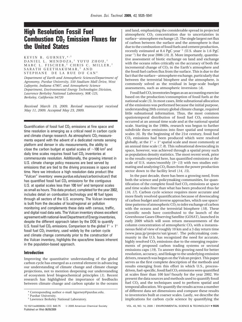
MethodsData Sources. The Vulcan U.S. fossil fuel CO2 emissionsinventory is constructed from seven primary data sets withadditional data used to shape the space/time distribution.A schematic is shown in Figure 1. A detailed description ofthe data sources, processing, and space/time allocation areprovided in Supporting Information [SI Text 1]. The followingis a summary of the Vulcan inventory methods.

The point, nonpoint, and airport data files come from theEnvironmental Protection Agency’s (EPA) National EmissionsInventory (NEI) for the year 2002 which is a comprehensiveinventory of all criteria air pollutants (CAPs) and hazardousair pollutants (HAPs) across the United States (24).

Point sources are stationary emitting sources identifiedto a geocoded location and comprise entities such asindustrial facilities in which emissions exit through a stackor identifiable exhaust feature (25, 26). The area or nonpointsource emissions (dominated by residential and commercialactivity) are stationary sources that are not inventoried atthe facility level and represent diffuse emissions within anindividual U.S. county reported as annual totals. The airportsource includes emissions associated with geocoded airportlocations (3865 facilities) and represent takeoff/landing cycle,taxiing, idling, and related aircraft activities on an annualbasis though some airports report emissions only duringsummer months (27). In all three of these categories, weutilize the reported CO emissions.

Emissions due to aircraft, beyond the takeoff/landing cycleand emissions captured in the NEI airport database, are takendirectly from the Aero2K aircraft CO2 emissions inventory,defined on a global three-dimensional 1° × 1° degree grid(28).

Because of the reliability of direct CO2 monitoring andthe need for fine time resolution data, we utilize CO2

emissions available at electrical generating units (EGUs)reported to the EPA’s Clean Air Market Division (CAMD)(United States Environmental Protection Agency, Clean AirMarkets - Data and Maps, http://camddataandmaps.epa.gov/

gdm/index.cfm, accessed June 10, 2008) under Part 75 of theClean Air Act (39). This data contains a large number offacilities that utilize Emission Tracking System/ContinuousEmissions Monitoring systems (ETS/CEMs), widely consid-ered the most accurate for CO2 emissions estimation at thesefacilities (15).

The onroad mobile emissions are based on a combinationof county-level data and standard internal combustion enginestochiometry. The county-level data comes from the NationalMobile Inventory Model (NMIM) County Database (NCD)for 2002 which quantifies the vehicle miles traveled in acounty by month, specific to vehicle class and road type (29).The Mobile6.2 combustion emissions model is used togenerate CO2 emission factors on a per mile basis given inputssuch as fleet information, temperature, fuel type, and vehiclespeed (30, 31).

Nonroad emissions are structured similarly to the onroadmobile emissions data and consist of mobile sources that donot travel on designated roadways. These data, retrieved fromthe NMIM NCD, have a space/time resolution of county/month and are reported as activity (number of hour/monthvehicle runs), population, and a CO2 emission factor specificto vehicle class (27, 32).

Emissions Calculation. For data sets that do not directlyprovide CO2 emissions, CO and CO2 emission factors areused. These factors are specific to the combustion processand the 48 fuels tracked in the Vulcan system. CO emissionfactors are often supplied in the incoming data sets but areoften missing or inconsistent with independent data. In manycases, therefore, standard emission factor databases are usedto assign values to each combustion technology/fuel com-bination (Technology Transfer Network Clearinghouse forInventories & Emissions Factor, WebFIRE, December 2005,http://cfpub.epa.gov/oarweb/index.cfm?action)fire.main,accessed 06/10/08). (33, 24). Where standard factors are notavailable, default emission factors are used (see SupportingInformation, SI text 1 and SI Tables 1 and 2).

Emission factors for CO2 are based on the fuel carboncontent and assume a gross calorific value or high heatingvalue, as this is the convention most commonly used in theU.S. and Canada (35). The basic process by which CO2

emissions are created is as follows:

FIGURE 1. Data sources, incoming/outgoing resolution, conditioning data sets, and processing details used in the Vulcan inventoryconstruction.

5536 9 ENVIRONMENTAL SCIENCE & TECHNOLOGY / VOL. 43, NO. 14, 2009

where C is the emitted amount of carbon, PE is the equivalentamount of uncontrolled criteria pollutant emissions (COemissions), p is the combustion process (e.g., industrial 10MMBTU boiler, industrial gasoline reciprocating turbine), fis the fuel type (e.g., natural gas or bituminous coal), PF isthe emission factor associated with the criteria pollutant,and CF is the emission factor associated with CO2. Percentoxidation level is embedded in the CO2 emission factor.

Spatial/Temporal Downscaling. For those data sourcesthat are not geocoded (mobile and nonpoint sources),allocation of emissions in space is performed through theuse of additional data sets. Downscaling of the residentialand commercial emissions in addition to the small amountof industrial sector emissions reported in the nonpoint NEIfiles are performed through use of U.S.Census tract-level (aU.S. Census tract is a geographic unit, smaller or equal to aU.S. county, defined for the purpose of taking a census) spatialsurrogates prepared by the EPA (36).

Onroad emissions are also spatially downscaled from thecounty level by allocating the hourly/county/road/vehicle-specific CO2 emissions onto roadways using a GIS road atlas(NTAD 2003 a collection of spatial data for use in GIS-basedapplications, United States. Bureau of Transportation Sta-tistics, www.worldcat.org/oclc/52933703&referer)one_hit).The monthly/county/road/vehicle-specific CO2 emissions arefurther subdivided in time using weight in motion (WIM)data obtained from the San Jose Valley traffic department(37).

Temporal downscaling to monthly time incrementsincrements by state for the residential and commercial sectorwas performed for the nonpoint data sources by state andsector. Data on state-level, sector-based natural gas deliveredto consumers from the DOE/EIA (38) was used to constructmonthly fractions for the year 2002.

In order to facilitate atmospheric transport modeling, allof these emission sources are placed onto a common 10 km× 10 km grid. Geocoded sources are evenly spread across theresident grid cell while onroad sources are broken at theedges of the grid cells and summed into the cells to whichthey belong. Nonpoint sources are downscaled from theCensus tract to 10 km via area-based weighting.

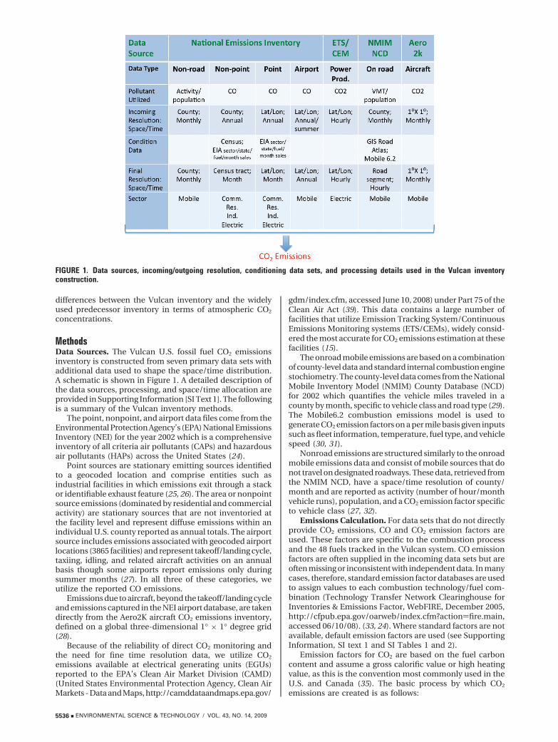
Results and DiscussionFigure 2 shows the Vulcan total 2002 U.S. fossil fuel CO2

emissions, represented on a 10 km × 10 km grid. Emissionsare most readily associated with population centers, butinterstate highways and concentrations of industrial activityare also evident. Because the incoming data represents amixture of spatial resolution, the gridded 10 km emissionsmap has both a background palette of uniform county-levelemissions and higher resolution points and line sources. Thisreflects data that was reported at geocoded points, data thatwas reported at the county level but downscaled to the censustract level, and data which could not be further downscaledfrom the county scale. This last category shows up asemissions evenly distributed over county areas. This isparticularly noticeable in the Plains states and intermountainWest, where county sizes are large, population is low, andfewer industrial and electric production point sources exist.

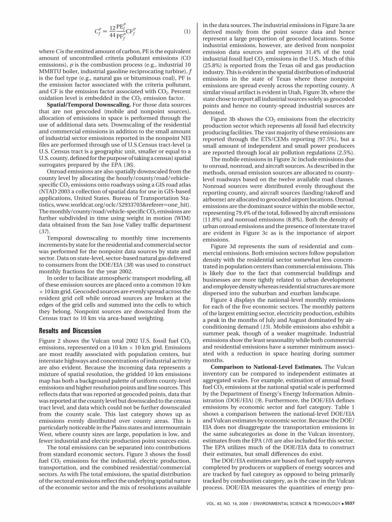
The total emissions can be separated into contributionsfrom standard economic sectors. Figure 3 shows the fossilfuel CO2 emissions for the industrial, electric production,transportation, and the combined residential/commercialsectors. As with Fhe total emissions, the spatial distributionof the sectoral emissions reflect the underlying spatial natureof the economic sector and the mix of resolutions available

in the data sources. The industrial emissions in Figure 3a arederived mostly from the point source data and hencerepresent a large proportion of geocoded locations. Someindustrial emissions, however, are derived from nonpointemission data sources and represent 31.4% of the totalindustrial fossil fuel CO2 emissions in the U.S.. Much of this(25.8%) is reported from the Texas oil and gas productionindustry. This is evident in the spatial distribution of industrialemissions in the state of Texas where these nonpointemissions are spread evenly across the reporting county. Asimilar visual artifact is evident in Utah, Figure 3b, where thestate chose to report all industrial sources solely as geocodedpoints and hence no county-spread industrial sources aredenoted.

Figure 3b shows the CO2 emissions from the electricityproduction sector which represents all fossil fuel electricityproducing facilities. The vast majority of these emissions arereported through the ETS/CEMs reporting (97.5%), but asmall amount of independent and small power producersare reported through local air pollution regulations (2.5%).

The mobile emissions in Figure 3c include emissions dueto onroad, nonroad, and aircraft sources. As described in themethods, onroad emission sources are allocated to county-level roadways based on the twelve available road classes.Nonroad sources were distributed evenly throughout thereporting county, and aircraft sources (landing/takeoff andairborne) are allocated to geocoded airport locations. Onroademissions are the dominant source within the mobile sector,representing 79.4% of the total, followed by aircraft emissions(11.8%) and nonroad emissions (8.8%). Both the density ofurban onroad emissions and the presence of interstate travelare evident in Figure 3c as is the importance of airportemissions.

Figure 3d represents the sum of residential and com-mercial emissions. Both emission sectors follow populationdensity with the residential sector somewhat less concen-trated in population centers than commercial emissions. Thisis likely due to the fact that commercial buildings andbusinesses are more tightly related to urban developmentand employee density whereas residential structures are moredispersed into the suburban and exurban landscape.

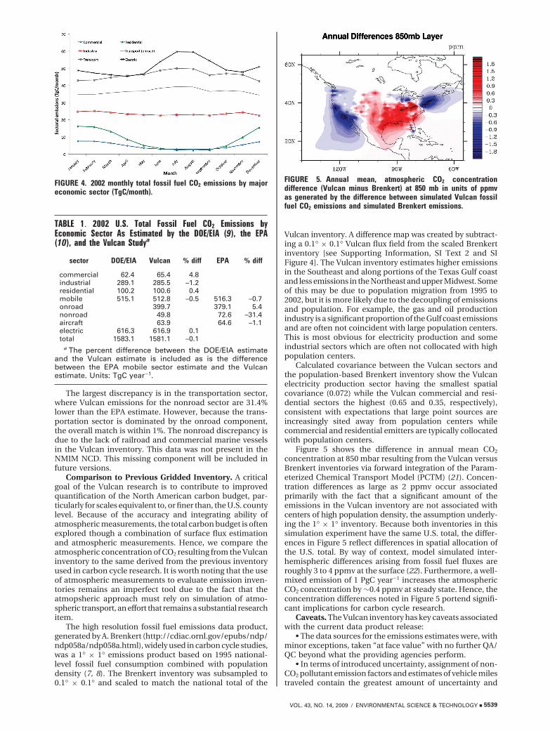
Figure 4 displays the national-level monthly emissionsfor each of the five economic sectors. The monthly patternof the largest emitting sector, electricity production, exhibitsa peak in the months of July and August dominated by air-conditioning demand (15). Mobile emissions also exhibit asummer peak, though of a weaker magnitude. Industrialemissions show the least seasonality while both commercialand residential emissions have a summer minimum associ-ated with a reduction in space heating during summermonths.

Comparison to National-Level Estimates. The Vulcaninventory can be compared to independent estimates ataggregated scales. For example, estimation of annual fossilfuel CO2 emissions at the national spatial scale is performedby the Department of Energy’s Energy Information Admin-istration (DOE/EIA) (9). Furthermore, the DOE/EIA definesemissions by economic sector and fuel category. Table 1shows a comparison between the national-level DOE/EIAand Vulcan estimates by economic sector. Because the DOE/EIA does not disaggregate the transportation emissions inthe same subcategories as done in the Vulcan inventory,estimates from the EPA (10) are also included for this sector.The EPA utilizes much of the DOE/EIA data to constructtheir estimates, but small differences do exist.

The DOE/EIA estimates are based on fuel supply surveyscompleted by producers or suppliers of energy sources andare tracked by fuel category as opposed to being primarilytracked by combustion category, as is the case in the Vulcanprocess. DOE/EIA measures the quantities of energy pro-

C fP ) 12

44

PEfP

PFfP

CFfP (1)

VOL. 43, NO. 14, 2009 / ENVIRONMENTAL SCIENCE & TECHNOLOGY 9 5537

duced or supplied to the market. At the national/annual scale,very small differences might be expected to occur whencomparing the DOE/EIA surveys to the Vulcan estimates.For example, the DOE/EIA does require balancing items inorder to balance the supply and consumption of natural gas,

and these can be on the order of 0.5 to 1% (20). Furthermore,supply and ultimate combustion of fuel may be differentdue to changes in stockpiling from one year to the next andassumptions about noncombustion oxidation of fossil fuels.This is particularly relevant for liquid petroleum fuel.

FIGURE 2. Total contiguous U.S. fossil fuel CO2 emissions for the year 2002 represented on a 10 km × 10 km grid (units: log10 GgC100 km-2 year-1).

FIGURE 3. Contiguous U.S. fossil fuel CO2 emissions from the (a) industrial sector (log10 GgC 100 km-2 year-1); (b) the electricityproduction sector (log10 GgC facility-1 year-1); (c) the transportation sector (log10 GgC km-1 year-1 for onroad, log10 GgC facility-1

year-1 for air transport, log10 GgC 100 km-2 year-1 for nonroad); (d) the sum of the commercial and residential sectors (log10 GgC 100km-2 year-1).


The largest discrepancy is in the transportation sector,where Vulcan emissions for the nonroad sector are 31.4%lower than the EPA estimate. However, because the trans-portation sector is dominated by the onroad component,the overall match is within 1%. The nonroad discrepancy isdue to the lack of railroad and commercial marine vesselsin the Vulcan inventory. This data was not present in theNMIM NCD. This missing component will be included infuture versions.

Comparison to Previous Gridded Inventory. A criticalgoal of the Vulcan research is to contribute to improvedquantification of the North American carbon budget, par-ticularly for scales equivalent to, or finer than, the U.S. countylevel. Because of the accuracy and integrating ability ofatmospheric measurements, the total carbon budget is oftenexplored though a combination of surface flux estimationand atmospheric measurements. Hence, we compare theatmospheric concentration of CO2 resulting from the Vulcaninventory to the same derived from the previous inventoryused in carbon cycle research. It is worth noting that the useof atmospheric measurements to evaluate emission inven-tories remains an imperfect tool due to the fact that theatmopsheric approach must rely on simulation of atmo-spheric transport, an effort that remains a substantial researchitem.

The high resolution fossil fuel emissions data product,generated by A. Brenkert (http://cdiac.ornl.gov/epubs/ndp/ndp058a/ndp058a.html), widely used in carbon cycle studies,was a 1° × 1° emissions product based on 1995 national-level fossil fuel consumption combined with populationdensity (7, 8). The Brenkert inventory was subsampled to0.1° × 0.1° and scaled to match the national total of the

Vulcan inventory. A difference map was created by subtract-ing a 0.1° × 0.1° Vulcan flux field from the scaled Brenkertinventory [see Supporting Information, SI Text 2 and SIFigure 4]. The Vulcan inventory estimates higher emissionsin the Southeast and along portions of the Texas Gulf coastand less emissions in the Northeast and upper Midwest. Someof this may be due to population migration from 1995 to2002, but it is more likely due to the decoupling of emissionsand population. For example, the gas and oil productionindustry is a significant proportion of the Gulf coast emissionsand are often not coincident with large population centers.This is most obvious for electricity production and someindustrial sectors which are often not collocated with highpopulation centers.

Calculated covariance between the Vulcan sectors andthe population-based Brenkert inventory show the Vulcanelectricity production sector having the smallest spatialcovariance (0.072) while the Vulcan commercial and resi-dential sectors the highest (0.65 and 0.35, respectively),consistent with expectations that large point sources areincreasingly sited away from population centers whilecommercial and residential emitters are typically collocatedwith population centers.

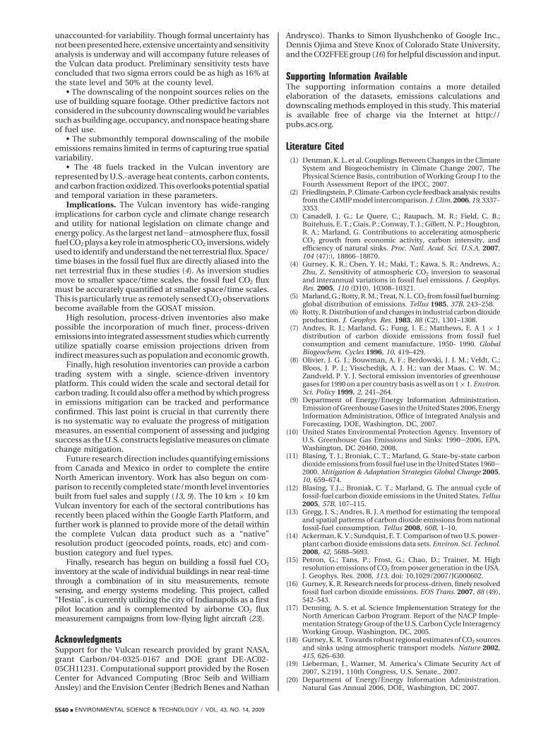
Figure 5 shows the difference in annual mean CO2

concentration at 850 mbar resulting from the Vulcan versusBrenkert inventories via forward integration of the Param-eterized Chemical Transport Model (PCTM) (21). Concen-tration differences as large as 2 ppmv occur associatedprimarily with the fact that a significant amount of theemissions in the Vulcan inventory are not associated withcenters of high population density, the assumption underly-ing the 1° × 1° inventory. Because both inventories in thissimulation experiment have the same U.S. total, the differ-ences in Figure 5 reflect differences in spatial allocation ofthe U.S. total. By way of context, model simulated inter-hemispheric differences arising from fossil fuel fluxes areroughly 3 to 4 ppmv at the surface (22). Furthermore, a well-mixed emission of 1 PgC year-1 increases the atmosphericCO2 concentration by ∼0.4 ppmv at steady state. Hence, theconcentration differences noted in Figure 5 portend signifi-cant implications for carbon cycle research.

Caveats. The Vulcan inventory has key caveats associatedwith the current data product release:

• The data sources for the emissions estimates were, withminor exceptions, taken “at face value” with no further QA/QC beyond what the providing agencies perform.

• In terms of introduced uncertainty, assignment of non-CO2 pollutant emission factors and estimates of vehicle milestraveled contain the greatest amount of uncertainty and

FIGURE 4. 2002 monthly total fossil fuel CO2 emissions by majoreconomic sector (TgC/month).

TABLE 1. 2002 U.S. Total Fossil Fuel CO2 Emissions byEconomic Sector As Estimated by the DOE/EIA (9), the EPA(10), and the Vulcan Studya

sector DOE/EIA Vulcan % diff EPA % diff

commercial 62.4 65.4 4.8industrial 289.1 285.5 –1.2residential 100.2 100.6 0.4mobile 515.1 512.8 –0.5 516.3 –0.7onroad 399.7 379.1 5.4nonroad 49.8 72.6 –31.4aircraft 63.9 64.6 –1.1electric 616.3 616.9 0.1total 1583.1 1581.1 –0.1

a The percent difference between the DOE/EIA estimateand the Vulcan estimate is included as is the differencebetween the EPA mobile sector estimate and the Vulcanestimate. Units: TgC year-1.

FIGURE 5. Annual mean, atmospheric CO2 concentrationdifference (Vulcan minus Brenkert) at 850 mb in units of ppmvas generated by the difference between simulated Vulcan fossilfuel CO2 emissions and simulated Brenkert emissions.


unaccounted-for variability. Though formal uncertainty hasnot been presented here, extensive uncertainty and sensitivityanalysis is underway and will accompany future releases ofthe Vulcan data product. Preliminary sensitivity tests haveconcluded that two sigma errors could be as high as 16% atthe state level and 50% at the county level.

• The downscaling of the nonpoint sources relies on theuse of building square footage. Other predictive factors notconsidered in the subcounty downscaling would be variablessuch as building age, occupancy, and nonspace heating shareof fuel use.

• The submonthly temporal downscaling of the mobileemissions remains limited in terms of capturing true spatialvariability.

• The 48 fuels tracked in the Vulcan inventory arerepresented by U.S.-average heat contents, carbon contents,and carbon fraction oxidized. This overlooks potential spatialand temporal variation in these parameters.

Implications. The Vulcan inventory has wide-rangingimplications for carbon cycle and climate change researchand utility for national legislation on climate change andenergy policy. As the largest net land-atmosphere flux, fossilfuel CO2 plays a key role in atmospheric CO2 inversions, widelyused to identify and understand the net terrestrial flux. Space/time biases in the fossil fuel flux are directly aliased into thenet terrestrial flux in these studies (4). As inversion studiesmove to smaller space/time scales, the fossil fuel CO2 fluxmust be accurately quantified at smaller space/time scales.This is particularly true as remotely sensed CO2 observationsbecome available from the GOSAT mission.

High resolution, process-driven inventories also makepossible the incorporation of much finer, process-drivenemissions into integrated assessment studies which currentlyutilize spatially coarse emission projections driven fromindirect measures such as population and economic growth.

Finally, high resolution inventories can provide a carbontrading system with a single, science-driven inventoryplatform. This could widen the scale and sectoral detail forcarbon trading. It could also offer a method by which progressin emissions mitigation can be tracked and performanceconfirmed. This last point is crucial in that currently thereis no systematic way to evaluate the progress of mitigationmeasures, an essential component of assessing and judgingsuccess as the U.S. constructs legislative measures on climatechange mitigation.

Future research direction includes quantifying emissionsfrom Canada and Mexico in order to complete the entireNorth American inventory. Work has also begun on com-parison to recently completed state/month level inventoriesbuilt from fuel sales and supply (13, 9). The 10 km × 10 kmVulcan inventory for each of the sectoral contributions hasrecently been placed within the Google Earth Platform, andfurther work is planned to provide more of the detail withinthe complete Vulcan data product such as a “native”resolution product (geocoded points, roads, etc) and com-bustion category and fuel types.

Finally, research has begun on building a fossil fuel CO2

inventory at the scale of individual buildings in near real-timethrough a combination of in situ measurements, remotesensing, and energy systems modeling. This project, called“Hestia”, is currently utilizing the city of Indianapolis as a firstpilot location and is complemented by airborne CO2 fluxmeasurement campaigns from low-flying light aircraft (23).

AcknowledgmentsSupport for the Vulcan research provided by grant NASA,grant Carbon/04-0325-0167 and DOE grant DE-AC02-05CH11231. Computational support provided by the RosenCenter for Advanced Computing (Broc Seib and WilliamAnsley) and the Envision Center (Bedrich Benes and Nathan

Andrysco). Thanks to Simon Ilyushchenko of Google Inc.,Dennis Ojima and Steve Knox of Colorado State University,and the CO2FFEE group (16) for helpful discussion and input.

Supporting Information AvailableThe supporting information contains a more detailedelaboration of the datasets, emissions calculations anddownscaling methods employed in this study. This materialis available free of charge via the Internet at http://pubs.acs.org.

Literature Cited(1) Denman, K. L. et al. Couplings Between Changes in the Climate

System and Biogeochemistry in Climate Change 2007, ThePhysical Science Basis, contribution of Working Group I to theFourth Assessment Report of the IPCC, 2007.

(2) Friedlingstein, P. Climate-Carbon cycle feedback analysis: resultsfrom the C4MIP model intercomparison. J. Clim. 2006, 19, 3337–3353.

(3) Canadell, J. G.; Le Quere, C.; Raupach, M. R.; Field, C. B.;Buitehuis, E. T.; Ciais, P.; Conway, T. J.; Gillett, N. P.; Houghton,R. A.; Marland, G. Contributions to accelerating atmosphericCO2 growth from economic activity, carbon intensity, andefficiency of natural sinks. Proc. Natl. Acad. Sci. U.S.A. 2007,104 (47):), 18866–18870.

(4) Gurney, K. R.; Chen, Y. H.; Maki, T.; Kawa, S. R.; Andrews, A.;Zhu, Z. Sensitivity of atmospheric CO2 inversion to seasonaland interannual variations in fossil fuel emissions. J. Geophys.Res. 2005, 110 (D10), 10308–10321.

(5) Marland, G.; Rotty, R. M.; Treat, N. L. CO2 from fossil fuel burning:global distribution of emissions. Tellus 1985, 37B, 243–258.

(6) Rotty, R. Distribution of and changes in industrial carbon dioxideproduction. J. Geophys. Res. 1983, 88 (C2), 1301–1308.

(7) Andres, R. J.; Marland, G.; Fung, I. E.; Matthews, E. A 1 × 1distribution of carbon dioxide emissions from fossil fuelconsumption and cement manufacture, 1950- 1990. GlobalBiogeochem. Cycles 1996, 10, 419–429.

(8) Olivier, J. G. J.; Bouwman, A. F.; Berdowski, J. J. M.; Veldt, C.;Bloos, J. P. J.; Visschedijk, A. J. H.; van der Maas, C. W. M.;Zandveld, P. Y. J. Sectoral emission inventories of greenhousegases for 1990 on a per country basis as well as on 1 × 1. Environ.Sci. Policy 1999, 2, 241–264.

(9) Department of Energy/Energy Information Administration.Emission of Greenhouse Gases in the United States 2006, EnergyInformation Administration, Office of Integrated Analysis andForecasting, DOE, Washington, DC, 2007.

(10) United States Environmental Protection Agency. Inventory ofU.S. Greenhouse Gas Emissions and Sinks: 1990-2006, EPA,Washington, DC 20460, 2008.

(11) Blasing, T. J.; Broniak, C. T.; Marland, G. State-by-state carbondioxide emissions from fossil fuel use in the United States 1960-2000. Mitigation & Adaptation Strategies Global Change 2005,10, 659–674.

(12) Blasing, T.J.,; Broniak, C. T.; Marland, G. The annual cycle offossil-fuel carbon dioxide emissions in the United States. Tellus2005, 57B, 107–115.

(13) Gregg, J. S.; Andres, R. J. A method for estimating the temporaland spatial patterns of carbon dioxide emissions from nationalfossil-fuel consumption. Tellus 2008, 60B, 1–10.

(14) Ackerman, K. V.; Sundquist, E. T. Comparison of two U.S. power-plant carbon dioxide emissions data sets. Environ. Sci. Technol.2008, 42, 5688–5693.

(15) Petron, G.; Tans, P.; Frost, G.; Chao, D.; Trainer, M. Highresolution emissions of CO2 from power generation in the USA.J. Geophys. Res. 2008, 113, doi: 10.1029/2007/JG000602.

(16) Gurney, K. R. Research needs for process-driven, finely resolvedfossil fuel carbon dioxide emissions. EOS Trans. 2007, 88 (49),542–543.

(17) Denning, A. S. et al. Science Implementation Strategy for theNorth American Carbon Program. Report of the NACP Imple-mentation Strategy Group of the U.S. Carbon Cycle InteragencyWorking Group, Washington, DC, 2005.

(18) Gurney, K. R. Towards robust regional estimates of CO2 sourcesand sinks using atmospheric transport models. Nature 2002,415, 626–630.

(19) Lieberman, J., Warner, M. America’s Climate Security Act of2007, S.2191, 110th Congress, U.S. Senate., 2007.

(20) Department of Energy/Energy Information Administration.Natural Gas Annual 2006, DOE, Washington, DC 2007.


(21) Kawa, S. R., Erickson, D. J., III. Pawson, S., Zhu, Z. Global CO2

transport simulations using meteorological data from the NASAdata assimilation system, 2004, J. Geophys. Res., 109 (D18312),doi: 10.1029/2004JD004554.

(22) Denning, A. S.; Fung, I. Y.; Randall, D. Latitudinal gradient ofatmospheric CO2 due to seasonal exchange with land biota.Nature 1995, 376, 240–243.

(23) Ross, K., Shepson, P., Stirm, B., Karion, A., Sweeney, C., Gurney,K., Aircraft-based measurements of the carbon footprint ofIndianapolis. Environ. Sci. Technol. 2009, submitted.

(24) United States Environmental Protection Agency. Emissions Inven-tory Guidance for Implementation of Ozone and Particulate MatterNational Ambient Air Quality Standards (NAAQS and RegionalHaze Regulations), EPA, Research Triangle Park, NC, 2005.

(25) United States Environmental Protection Agency. Documentationfor the Final 2002 Point Source National Emissions Inventory,Emission Inventory and Analysis Group, Air Quality and AnlysisDivision, EPA, Research Triangle Park, NC, 2006.

(26) Eastern Research Group, Inc. Introduction to Stationary PointSource Emissions Inventory Development, Volume II, Chapter1, prepared for Point Sources Committee, Emission InventoryImprovement Program, 2001.

(27) United States Environmental Protection Agency. Documentationfor Aircraft, Commercial Marine Vessel, Locomotive, and OtherNonroad Components of the National Emissions Inventory,Volume I - Methodology, EPA, Research Triangle Park, NC, 2005.

(28) Eyers, C. J.; Norman, P.; Middel, J.; Plohr, M.; Michot., S.;Atkinson, K.; Christou, R. A. AERO2k Global Aviation EmissionsInventories for 2002 and 2025, Center for Air Transport and theEnvironment, QINETIQ/04/01113, 2004.

(29) United States Environmental Protection Agency. EPA’s NationalMobile Inventory Model (NMIM), A consolidated emissionsmodeling system for MOBILE6 and NONROAD, EPA, Wash-ington, DC, 2005.

(30) United States Environmental Protection Agency. Fleet Char-acterization Data for MOBILE6: Development and Use of AgeDistributions, Average Annual Mileage Accumulation Rates, andProjected Vehicle Counts for Use in MOBILE6, EPA, Washington,DC, 2001.

(31) Harrigton, W. A Behavioral Analysis of EPA’s MOBILE EmissionFactor Model, Discussion Paper 98-47, Resources for the Future:Washington, DC, 1998.

(32) United States Environmental Protection Agency. User’s Guidefor the Final NONROAD 2005 Model, Assessment and Standards,EPA, Washington DC, 2005.

(33) United States Environmental Protection Agency. Proceduresfor Preparing Emission Factor Documents, EPA, ResearchTriangle Park, NC,November, EPA-454/R-95-015 Revised, 1997.

(34) United States Environmental Protection Agency. Draft DetailedProcedures for Preparing Emissions Factors, EPA, ResearchTriangle Park, NC, 2006.

(35) URS. Greenhouse Gas Emission Factor Review, Final TechnicalMemorandum, URS Corporation, Austin, TX, 2003.

(36) DynTel. Spatial Allocation Information Improvements, TechnicalMemorandum, Review of Existing Data Sources, Work Order25.6, 2002.

(37) Marr, L. C.; Black, D. R.; Harley, R. A. Formation of photochemicalair pollution in central California - 1. Development of a revisedmotor vehicle emission inventory. J. Geophys. Res.-A: Space Phys.2002, 107 (D5-D6), 4047–4056.

(38) Department of Energy/Energy Information Administration.Natural Gas Monthly February 2003, DOE, Washington, DC,2003.

(39) United States Environmental Protection Agency. Plain EnglishGuide to the Part 75 Rule, EPA: Washington, DC, 2005.

ES900806C
