High-resolution calcareous nannoplankton palaeoecology as a proxy for small-scale environmental changes in the Early Miocene

Marine Micropaleontology 111 (2014) 53–65

Contents lists available at ScienceDirect

Marine Micropaleontology

j ourna l homepage: www.e lsev ie r .com/ locate /marmicro

Research paper

High-resolution calcareous nannoplankton palaeoecology as a proxy forsmall-scale environmental changes in the Early Miocene

Gerald Auer a,⁎, Werner E. Piller a, Mathias Harzhauser b

a Institute for Earth Sciences, University of Graz, NAWI Graz, Heinrichstrasse 26, 8010 Graz, Austriab Natural History Museum Vienna, Geological–Paleontological Department, Burgring 7, 1010 Vienna, Austria

⁎ Corresponding author at: University of Graz, InstituteHeinrichstrasse 26, 8010 Graz, Styria, Austria. Tel.: +43380 9871.

E-mail addresses: [email protected] (G. Auer(W.E. Piller), [email protected] (M

http://dx.doi.org/10.1016/j.marmicro.2014.06.0050377-8398/© 2014 The Authors. Published by Elsevier B.V

a b s t r a c t

Article history:Received 26 June 2013Received in revised form 5 June 2014Accepted 15 June 2014Available online 20 June 2014

Keywords:High-resolutionPalaeoecologyCalcareous nannoplanktonSmall-scale environmental changeEarly MioceneNorth Alpine Foreland Basin

Within a 5.5-m-thick succession of upper Burdigalian (CNP-zone NN4) shallow neritic sediments from the NorthAlpine Foreland Basin in Lower Austria a high-resolution section of finely laminated sedimentwith a thickness of940.5 mmwas logged. The section was continuously sampled, resulting in 100 samples, covering a thickness of~10 mm each. An integrated approach was applied to these samples in order to study proxy records includingcalcareous nannoplankton, geochemical and geophysical data.Multivariate statistics on the autochthonous assemblagewere used to evaluate the ecological preferences of eachtaxon and to rule out possible contamination of the signal by taphonomic processes. In order to assess changes inthe assemblage composition throughout the section, three taphogroups were defined using both the autochtho-nous and allochthonous nannofossils. Based on the distribution of these taphogroups five distinct intervals weredefined that are indicative of centennial to decadal changes in palaeoenvironmental conditions. Combining theseresults with other proxies (geochemistry, geophysics) we were able to reconstruct short-term, small-scale vari-ations in terms of temperature, primary productivity, bottomwater oxygenation, organicmatter flux, freshwaterinflux and changes in relative sea level in a highly dynamic shallow marine setting.This study represents thefirst such high-resolution analysis performed on amarine succession of late Burdigalianage. It is also a first attempt to analyse outcrop data on such a high-resolution, sub-Milankovitch scale, with re-spect to calcareous nannoplankton in conjunction with geochemical and sedimentological data.

© 2014 The Authors. Published by Elsevier B.V. This is an open access article under the CC BY license(http://creativecommons.org/licenses/by/3.0/).

1. Introduction

Althoughgeosciences are amajor player in the climate change debate,high-resolution palaeoecological and palaeoenvironmental studies on adecadal to millennial scale are mostly restricted to geologically youngsediments, in particular, to those of the Quaternary (e.g., Meyers andArnaboldi, 2005; Kloosterboer-van Hoeve et al., 2006; Mudie et al.,2007; Sprovieri et al., 2012). Undisturbed and laminated sedimentswith-out bioturbation are best suited for this type of study. Examples from thepre-Pleistocene originate mostly from palaeolakes where laminated orvarved sediments are relatively abundant (Lindqvist and Lee, 2009;Lenz et al., 2010; Gross et al., 2011; Kern et al., 2012; 2013). In pre-Pleistocene marine sediments palaeoecological studies based onpalaeobiological proxies have never been performed on a comparableresolution. Principally, only a few proxies are applicable in high-resolution studies. In addition to geochemical and geophysical proxies

for Earth Sciences, NAWI Graz,316 380 8727; fax: +43 316

), [email protected]. Harzhauser).

. This is an open access article under

only microfossils can be used for this type of study because of theirsmall size. Calcareous nannofossils fulfil these requirements best, howev-er, they are mostly well known for their excellent stratigraphic potentialin the Mesozoic and Cenozoic, which is expressed in standard biostrati-graphic zonations (e.g., Bown, 1998 and references therein). Although adeep understanding of their ecology is still lacking, general inferenceson the ecological preferences ofmany taxa can still be drawn froma care-ful study of nannoplankton literature data (e.g., Ziveri et al., 2004). Com-bined with statistical methods, especially cluster analysis, these datashow promise as a powerful tool for ecological interpretations ofnannofossil assemblages (e.g., Spezzaferri and Ćorić, 2001; Couapelet al., 2007), even with the severe limitations imposed on the currentknowledge of nannoplankton ecology.

In particular, for high-resolution studies calcareous nannoplanktonhave only been used in Pleistocene to Holocene deposits (Negri andGiunta, 2001; Álvarez et al., 2005; Mertens et al., 2009). InMiocene sur-face outcrops it has never been studied with a decadal to millennialresolution.

In order to demonstrate that calcareous nannoplankton assemblagesare an excellent proxy for high-resolution palaeoenvironmental recon-structions we use laminated marine sediments of late Burdigalian agefrom the Central Paratethys with high sedimentation rates (estimated

the CC BY license (http://creativecommons.org/licenses/by/3.0/).

54 G. Auer et al. / Marine Micropaleontology 111 (2014) 53–65

as 500mm kyr−1 based on calculations in similar settings; Hoheneggerand Wagreich, 2011). Together with the distribution of nannoplanktonassemblages we also analyse geochemical and sedimentological prox-ies. The results show that Early Miocene coccolithophores were highlysensitive to changes in environmental conditions and thus allow ecolog-ical reconstructions with a high temporal resolution.

2. Geological setting

The studied section is located in an abandoned clay pit ESE of Laa ander Thaya in Lower Austria (48° 43′ 0.84″N, 16° 24′ 45.18″ E), about50 km north of Vienna (Fig. 1). Palaeogeographically, the area of depo-sition was located within the North Alpine Foreland Basin (NAFB),whichwas part of the Central Paratethys during the Oligocene andMio-cene (Harzhauser and Piller, 2007; Piller et al., 2007). In the studied claypit sediments of the Laa Formation are exposed. This formation is anupper Burdigalian lithostratigraphic unit, with a thickness of up to1000 m (as recorded in well logs near the outcrop), which displays ageneral coarsening upward trend and corresponds to the lower andmiddle Karpatian of the regional chronostratigraphic scheme of theCentral Paratethys (Piller et al., 2007; Fig. 2). The total geochronologicrange of the Karpatian is 17.2–15.9 Ma (Grunert et al., 2010b; 2012;Fig. 2). The Laa Formation unconformably overlies Ottnangian sedi-ments (Nehyba and Petrová, 2000; Roetzel and Schnabel, 2002;Adamek et al., 2003). The marine sediments of the Laa Formation arecomposed of calcareous, laminated, greenish to brownish grey, mica-ceous, silty shales with thin fine sand intercalations (Roetzel andSchnabel, 2002). Dellmour and Harzhauser (2012) suggest an age of c.17.2–16.5 Ma for the Laa Formation. Due to the isolated occurrence ofthe studied outcrop no precise position of these sediments within theformation can be given.

Benthic foraminiferal assemblages and the P/B-ratio indicate waterdepths between 100 and 200 m (inner to outer shelf environment)(Spezzaferri and Ćorić, 2001). Sandy intercalations are interpreted asepisodic storm events (Roetzel and Schnabel, 2002). Nannoplankton as-semblages indicate cool to temperate, nutrient-rich surface-water con-ditions that triggered the formation of dysoxic bottom waters(Spezzaferri and Ćorić, 2001; Spezzaferri et al., 2002). Upwelling condi-tions have been reported for the study area as well as for other parts ofthe North Alpine Foreland Basin (Spezzaferri and Ćorić, 2001; Roetzelet al., 2007).

The entire Laa Formation is dated toNeogeneNannoplankton Zone 4(NN4) (Martini, 1971) orMediterraneanNeogene Nannoplankton Zone

Tha

CZ

DE

CZ

AUSTRIA

ITCH

SI

HU

ViennaLAA a. d. Thaya

Fig. 1. Location map showing the geographical position of the clay pit near

4a (MNN4a; Fornaciari and Rio, 1996; Fornaciari et al., 1996)(Spezzaferri and Ćorić, 2001; Spezzaferri et al., 2002; Adamek et al.,2003; Svabenicka et al., 2003). Both of which correspond to CalcareousNannofossil Miocene biozone 6 (CNM6) of Backman et al. (2012). Thecalcareous nannofossil assemblages are of low to moderate diversityand contain a very high amount (up to 45%) of reworked (Palaeogeneand Cretaceous) specimens (Spezzaferri and Ćorić, 2001).

3. Material and methods

3.1. Sampling and field methods

The exposed sedimentary succession in the clay pit has an overallthickness of 5.5 m and consists of finely laminated blue-grey to green-grey clayswith intercalations offine sand and silt lenses (Fig. 3). Lamina-tion varies on a sub-millimetre to centimetre scale. The intercalated siltand fine sand layers reach a thickness of up to 50 mm and decrease infrequency and thickness towards the top of the succession and frequent-ly show well-preserved current ripples. The sediment is mostly free ofbioturbation aswell as macrofossils. Natural gamma radiation andmag-netic susceptibility were logged continuously for the whole outcrop,using a portable scintillation counter (Heger–Breitband–Gammasonde)and a portable magnetic susceptibility meter (Exploranium KT-9), re-spectively (Fig. 3).

Starting at 3.06m above the base of the succession a high-resolutionsection was studied with an overall thickness of 940.5 mm (Fig. 3). 100layers were logged and sampled by completely removing a substantialportion (N300 g) of each layer. The top of each newly exposed layerwas thoroughly cleaned of debris before sampling. This top down ap-proach was applied because it allowed clean retrieval of all samples.For subsequent analyses a portion of each sample was extracted afterthoroughly homogenising the sediment from the respective layer.

The high-resolution section is situated in a relatively undisturbed se-quence of finely laminated clays with some intercalations of fine sandand silt. The intercalations increase in frequency and thickness in thetopmost part of the section and some show current ripples. Weak bio-turbation is only present in two successive layers of laminated claysnear the base of the section. Otherwise a clear lamination dominatesthe lower half of the section but becomes progressively less prominentto the top. Additionally, the layers become less clearly defined andwavy. This trend is coupled with a decrease in gamma ray intensityand magnetic susceptibility in the topmost part of the high-resolutionsection (Fig. 3).

ya

clay pit

AT

0 2.5km

B45

B46

LAA a. d. Thaya

Laa an der Thaya in Lower Austria where the studied section is located.

C6C

C6B

C6AA

C6A

C6

C5E

C5D

C5C

C5B

C5AD

C5AC

C5AB C5AA C5A

Aquitanian

Burdigalian

Langhian

Serravallian

Miocene

15

20 Ear

ly

Egerian

Eggenburgian

Ottnangian

Badenian

Sarmatian

NN1

NN2

NN3

NN4

NN5

NN6

CN1

CN2

CN3

CN4

Aq2

Bur1

Bur2

Bur3

Bur4

Bur5/Lan1

Ser1Ser2

Ser3

Tor1

23.0

20.4

15.97

13.82

Neo

gene

Aquitanian

Burdigalian

Langhian

Serravallian

15

20 Ear

ly

Egerian

Eggenburgian

Ottnangian

Badenian

Sarmatian

NN1

NN2

NN3

NN4

NN5

NN6

CN1

CN2

CN3

CN4

CN5

23.0

20.4

15.97

13.82

11.63 C5 NN7

SequenceStratigraphy

rd(3 order)Geomagnetic

PolarityAge/StageEpochPeriod

Age

(Ma

BP

) RegionalStages

(Central Paratethys)Calcareous

Nannofossils

Mid

dle

Karpatian16

14

13

12

17

18

19

21

22

23

Fig. 2. Global and regional Miocene chronostratigraphy and nannoplankton stratigraphy. Global chronostratigraphy follows Gradstein et al. (2012 and references therein). Sequence stra-tigraphy after Hardenbol et al. (1988). Regional stratigraphy of the Central Paratethys after Harzhauser and Piller (2007)with calibrated ages of theOttnangian andKarpatian after Grunertet al. (2010b) and Dellmour and Harzhauser (2012).

55G. Auer et al. / Marine Micropaleontology 111 (2014) 53–65

3.2. Sample preparation

Approximately 10 g of each of the 100 samples was powdered and0.1–0.15 g was analysed using a LECO CS230 for wt.% of total carbon(TC), sulphur and total organic carbon (TOC). Based on the TC andTOC the total inorganic carbon (TIC= TC− TOC) content was calculat-ed, which was then used to compute the calcite equivalent carbonatecontent using the stoichiometric formula (8.34 ∗ TIC) (Stax and Stein,1995; Grunert et al., 2010a). Additionally, the ratio of organic carbonto sulphur (C/S-ratio) was calculated (Berner and Raiswell, 1984).

Smear slideswere prepared for analysis of calcareous nannofossil as-semblages following the standard preparation methods of Bown andYoung (1998). We opted to leave the sediment untreated in order topreserve the original composition of the assemblages. To facilitate dis-aggregation they were ultrasonicated for 5 s before transfer of the sus-pension onto the coverslip. The slides were mounted using Eucit® andstudied with a standard light microscope at a magnification of 1000×under parallel and crossed nicols. Approximately 300 specimens werecounted in each sample. The assemblages were then analysed with re-spect to their similarity/dissimilarity to each other, as well as shifts inabundances of taxa over time.

3.3. Taxonomic remarks

The taxonomy used herein is largely based on Perch-Nielsen (1985a;1985b), Young (1998), Varol (1998) and Burnett (1998), supplementedby the Handbook of Calcareous Nannoplankton 1–5 (Aubry, 1984;1988; 1989; 1990; 1999) and the Nannotax website (Young et al.,2013). The revised taxonomy for the Paratethys by Galović and Young(2012) was also considered.

Specimens were identified to the species level wherever possible.Subsequently all identified taxawere grouped according to their record-ed stratigraphic range, in order to create a stratigraphic framework andquantify the amount of allochthonous taxa present in the assemblage.The autochthonous taxa were then analysed using multivariate statis-tics (cluster-analyses andnMDS) to reconstruct the palaeoenvironment.

The use of the terms allochthonous and autochthonous follows theguidelines of Martin (1999) regarding fossil assemblages.

The genus Reticulofenestra is a morphologically diverse andsomewhat poorly constrained coccolith taxon ranging from Eoceneto Recent (Young, 1998). For this study the general distinction ofYoung (1998) based on the placolith size was used: Reticulofenestraminuta b3 μm, Reticulofenestra haqii 3–5 μm, Reticulofenestrapseudoumbilicus N5 μm. The frequently applied distinction betweenmedium-sized reticulofenestrids (3–5 μm) with open and closedcentral areas (R. haqii (open) versus Reticulofenestra antarctica(closed)) (Wade and Bown, 2006) was not used because of thehigh amount of reworked and poorly preserved specimens. Other al-lochthonous taxa of the genus Reticulofenestra from the Palaeogenewere identified following the morphotype concept of Varol (1998).

3.4. Statistical treatment and analyses

The number of specimens per field of view in the light microscopewas used as a rough indicator of the total abundance of calcareousnannofossils in the samples. The arithmetic mean as well as the stan-dard deviation for the collected datasets were calculated using the per-centages of taxa within each sample. The Shannon–Wiener diversityindex, the dominance index and the species evenness (Shannon andWeaver, 1948; Sokal and Rohlf, 1995;Wade and Bown, 2006) were cal-culated using the statistics software PAST® (Hammer et al., 2001).

In order to ensure the normal distribution of the relative abun-dances, the studied dataset was transformed using the arcsine transfor-mation as outlined in Sokal and Rohlf (1995). The reason for using thistransformationmethodwas to generate awell-suited dataset for subse-quent statistical treatments.

In order to verify that allochthonous specimens of long ranging taxado not obscure the ecological signal of the autochthonous assemblage anR-mode analysis was performed. For this analysis both cluster analysis(Ward's-method) andnon-metricmultidimensional scaling (nMDS; Eu-clidean similarity measure) were applied (Hammer and Harper, 2006).

To determine assemblages a Q-mode cluster analysis was performedusing Ward's-method (Ward, 1963; Hammer and Harper, 2006). To

outcrop

1 m

2 m

3 m

4 m

5 m

clay withsilt layerssiltfine sand

with clay gypsum

lithology:

silt-fine sandalternation clayfine sand clay-silt

alternation current ripples

sedimentary structures:

lamination bioturbation

T-R cycles

- 0,04 0,08 0,12 0,160

magnetic susceptibility

3-point running average

32 40 48CPS

gamma-ray

3-point running average

+rel. sea level

HR-section1 m

0.75 m

0.5 m

0.25 m0.25 m

0 m

Fig. 3. Lithologs of the 5.5-metre-outcrop and the high-resolution section. Position of the HR-section within the 5.5-metre-section is indicated by the grey rectangle. Gamma-ray emissionandmagnetic susceptibility logs are shown as black lines. A threepoint runningmeanwas calculated for bothmeasurements and is shown asmirrored column for bothmeasurements. Thegamma-ray log was used to reconstruct changes in relative sea level.

56 G. Auer et al. / Marine Micropaleontology 111 (2014) 53–65

assess which taxa are primarily responsible for the differences betweenclusters, a similarity percentage analysis (SIMPER)was performedusingthe Bray–Curtis similaritymeasure (Bray and Curtis, 1957; Clarke, 1993;Hammer and Harper, 2006).

4. Results

4.1. Nannoplankton taphonomy

Of the 124 recorded taxa only 10 of them occur with a mean N1%.These represent an average of 78.64% (σ = 4.61) of the total assem-blage. In decreasing abundances the taxa are: Coccolithus pelagicus(34.52%; σ = 4.91), R. minuta (12.48%; σ = 4.95), Cyclicargolithusfloridanus (8.57%; σ = 3.23), Watznaueria barnesae (8.47%; σ = 3.07),R. haqii (5.76%; σ = 2.51), R. pseudoumbilicus (2.18%, σ = 1.19),

Reticulofenestra bisecta (2.04%; σ = 1.14), Prediscosphaera cretacea(1.72%; σ = 0.91), Cyclagelosphaera reinhardtii (1.72%; σ = 1.17) andLanternithus minutus (1.18%; σ= 0.85).

The remaining 114 taxa (b1%) represent on average 21.36%(σ = 4.61) of the total assemblage. Some accessory taxa, e.g.,Braarudosphaera bigelowii, Helicosphaera carteri and Sphenolithusmoriformis, show elevated abundances in certain samples.

Of all taxa recorded, only 24 occur within Zone MNN4a (see taxo-nomic list in the supplement). These represent an average of 67.86%(σ= 5.33) of the total assemblage. Some of them display a wide strat-igraphic range and thus likely contain specimens that are reworkedfrom Paleocene to Eocene sediments (see below). Such taxa areC. pelagicus, C. floridanus, as well as S. moriformis and R. minuta. Sincein such cases allochthonous specimens could not be readily distin-guished from autochthonous ones all specimens belonging to these

57G. Auer et al. / Marine Micropaleontology 111 (2014) 53–65

taxawere considered to be part of the autochthonous assemblage. How-ever, subsequent analyses indicate that the ecological signal of thesetaxa is largely unaffected by this partial contamination.

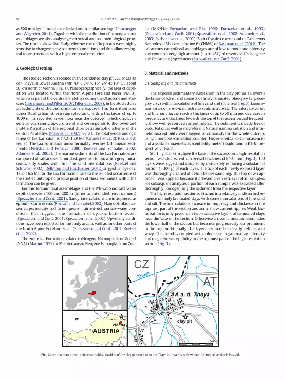
100 clearly allochthonous taxawere found: 41 taxa can be attributedto the Palaeogene, mainly Paleocene and Eocene and 59 were clearlyCretaceous (mainly Campanian to Maastrichtian). Palaeogene taxa in-clude R. bisecta, Reticulofenestra umbilica, L. minutus, Zygrhablithusbijugatus, as well as Cyclicargolithus luminis. The Cretaceous assemblageis dominated by W. barnesae, P. cretacea, C. reinhardtii, Miculastaurophora andMicula decussata. All allochthonous taxa were groupedtogether for subsequent statistical treatments as a proxy for terrigenousinput (Fig. 4).

4.2. Nannoplankton abundance and diversity

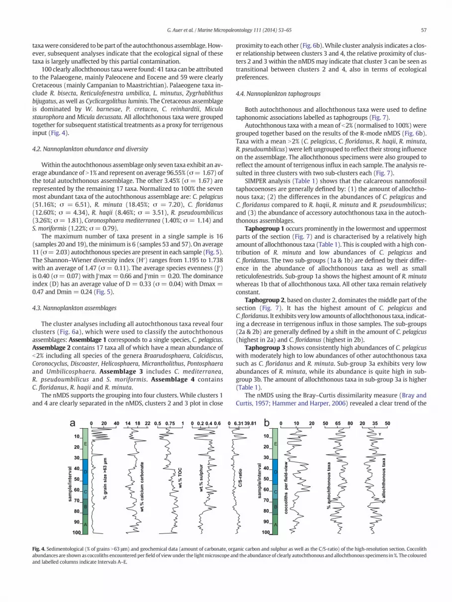
Within the autochthonous assemblage only seven taxa exhibit an av-erage abundance of N1% and represent on average 96.55% (σ= 1.67) ofthe total autochthonous assemblage. The other 3.45% (σ = 1.67) arerepresented by the remaining 17 taxa. Normalized to 100% the sevenmost abundant taxa of the autochthonous assemblage are: C. pelagicus(51.16%; σ = 6.51), R. minuta (18.45%; σ = 7.20), C. floridanus(12.60%; σ = 4.34), R. haqii (8.46%; σ = 3.51), R. pseudoumbilicus(3.26%; σ = 1.81), Coronosphaera mediterranea (1.40%; σ = 1.14) andS. moriformis (1.22%; σ = 0.79).

The maximum number of taxa present in a single sample is 16(samples 20 and 19), theminimum is 6 (samples 53 and 57). On average11 (σ= 2.03) autochthonous species are present in each sample (Fig. 5).The Shannon–Wiener diversity index (H′) ranges from 1.195 to 1.738with an average of 1.47 (σ = 0.11). The average species evenness (J′)is 0.40 (σ= 0.07) with J′max= 0.66 and J′min = 0.20. The dominanceindex (D) has an average value of D = 0.33 (σ = 0.04) with Dmax =0.47 and Dmin = 0.24 (Fig. 5).

4.3. Nannoplankton assemblages

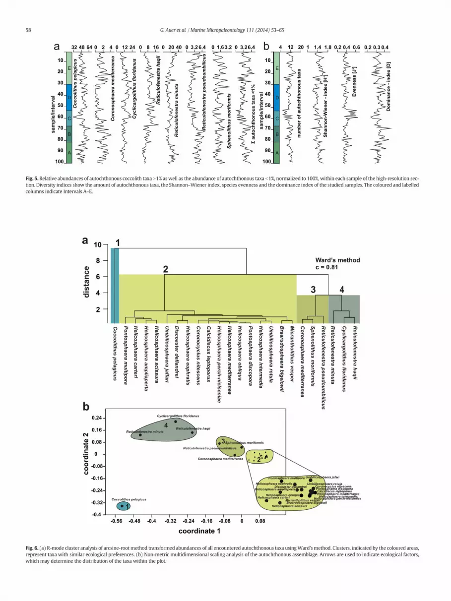
The cluster analyses including all autochthonous taxa reveal fourclusters (Fig. 6a), which were used to classify the autochthonousassemblages: Assemblage 1 corresponds to a single species, C. pelagicus.Assemblage 2 contains 17 taxa all of which have a mean abundance ofb2% including all species of the genera Braarudosphaera, Calcidiscus,Coronocyclus, Discoaster, Helicosphaera, Micrantholithus, Pontosphaeraand Umbilicosphaera. Assemblage 3 includes C. mediterranea,R. pseudoumbilicus and S. moriformis. Assemblage 4 containsC. floridanus, R. haqii and R. minuta.

The nMDS supports the grouping into four clusters. While clusters 1and 4 are clearly separated in the nMDS, clusters 2 and 3 plot in close

A

B

C

D

E

14 18 22

wt.%

cal

cium

car

bona

te

0.5 1 0 0.2 0.4 0.6

wt.%

sul

phur

00 40

% g

rain

siz

e >6

3 μm

20

wt.%

TO

C

0.75

10

20

30

40

50

60

70

80

90

100

sam

ple/

inte

rval

a

Fig. 4. Sedimentological (% of grains N63 μm) and geochemical data (amount of carbonate, orgabundances are shown as coccoliths encountered perfield of viewunder the lightmicroscope anand labelled columns indicate Intervals A–E.

proximity to each other (Fig. 6b).While cluster analysis indicates a clos-er relationship between clusters 3 and 4, the relative proximity of clus-ters 2 and 3 within the nMDSmay indicate that cluster 3 can be seen astransitional between clusters 2 and 4, also in terms of ecologicalpreferences.

4.4. Nannoplankton taphogroups

Both autochthonous and allochthonous taxa were used to definetaphonomic associations labelled as taphogroups (Fig. 7).

Autochthonous taxa with a mean of b2% (normalised to 100%) weregrouped together based on the results of the R-mode nMDS (Fig. 6b).Taxa with a mean N2% (C. pelagicus, C. floridanus, R. haqii, R. minuta,R. pseudoumbilicus)were left ungrouped to reflect their strong influenceon the assemblage. The allochthonous specimens were also grouped toreflect the amount of terrigenous influx in each sample. The analysis re-sulted in three clusters with two sub-clusters each (Fig. 7).

SIMPER analysis (Table 1) shows that the calcareous nannofossiltaphocoenoses are generally defined by: (1) the amount of allochtho-nous taxa; (2) the differences in the abundances of C. pelagicus andC. floridanus compared to R. haqii, R. minuta and R. pseudoumbilicus;and (3) the abundance of accessory autochthonous taxa in the autoch-thonous assemblages.

Taphogroup 1 occurs prominently in the lowermost and uppermostparts of the section (Fig. 7) and is characterised by a relatively highamount of allochthonous taxa (Table 1). This is coupled with a high con-tribution of R. minuta and low abundances of C. pelagicus andC. floridanus. The two sub-groups (1a & 1b) are defined by their differ-ence in the abundance of allochthonous taxa as well as smallreticulofenestrids. Sub-group 1a shows the highest amount of R. minutawhereas 1b that of allochthonous taxa. All other taxa remain relativelyconstant.

Taphogroup 2, based on cluster 2, dominates themiddle part of thesection (Fig. 7). It has the highest amount of C. pelagicus andC. floridanus. It exhibits very low amounts of allochthonous taxa, indicat-ing a decrease in terrigenous influx in those samples. The sub-groups(2a & 2b) are generally defined by a shift in the amount of C. pelagicus(highest in 2a) and C. floridanus (highest in 2b).

Taphogroup 3 shows consistently high abundances of C. pelagicuswith moderately high to low abundances of other autochthonous taxasuch as C. floridanus and R. minuta. Sub-group 3a exhibits very lowabundances of R. minuta, while its abundance is quite high in sub-group 3b. The amount of allochthonous taxa in sub-group 3a is higher(Table 1).

The nMDS using the Bray–Curtis dissimilarity measure (Bray andCurtis, 1957; Hammer and Harper, 2006) revealed a clear trend of the

Y

6.31 39.81

C/S

-rat

io

0 10 20

cocc

olith

s p

er fi

eld-

view

50 65

% a

utoc

htho

nous

taxa

20 35

% a

lloch

thon

ous

taxa

80 50

10

20

30

40

50

60

70

80

90

100

sam

ple/

inte

rval

b

A

B

C

D

E

anic carbon and sulphur as well as the C/S-ratio) of the high-resolution section. Coccolithd the abundance of clearly autochthonous and allochthonous specimens in %. The coloured

4 12 20 1 1.4 1.8 0.2 0.3 0.4

num

ber o

f aut

ocht

hono

us ta

xa

Shan

non-

Wie

ner -

inde

x [H

‘]

Dom

inan

ce -

inde

x [D

]

0.2 0.4 0.6

Even

ness

[J‘]

sam

ple/

inte

rval

32 48 64

Coc

colit

hus

pela

gicu

s

0 2 4

Cor

onos

phae

ra m

edite

rran

ea

0 12 24

Cyc

licar

golit

hus

florid

anus

0 8 16

Ret

icul

ofen

estr

a ha

qii

0 20 40

Ret

icul

ofen

estr

a m

inut

a

0 3.2 6.4

Ret

icul

ofen

estr

a ps

eudo

umbi

licus

0 1.63.2

Sphe

nolit

hus

mor

iform

is

0 3.26.4

Σ au

toch

thon

ous

taxa

<1%

10

20

30

40

50

60

70

80

90

100

sam

ple/

inte

rval

a b10

20

30

40

50

60

70

80

90

100A

B

C

D

E

A

B

C

D

E

Fig. 5. Relative abundances of autochthonous coccolith taxa N1% aswell as the abundance of autochthonous taxa b1%, normalized to 100%, within each sample of the high-resolution sec-tion. Diversity indices show the amount of autochthonous taxa, the Shannon–Wiener index, species evenness and the dominance index of the studied samples. The coloured and labelledcolumns indicate Intervals A–E.

10

8

6

4

2

dist

ance

Helicosphaera am

pliaperta

Helicosphaera carteri

Pontosphaera multipora

Coccolithus pelagicus

Helicosphaera scissura

Um

bilicosphaera jaffari

Discoaster deflandrei

Coronocyclus nitescens

Calcidiscus leptoporus

Helicosphaera perch-nielseniae

Helicosphaera m

editerranea

Helicosphaera obliqua

Pontosphaera discopora

Helicosphaera interm

edia

Um

bilicosphaera rotula

Braarudosphaera bigelow

ii

Micrantholithus vesper

Coronosphaera m

editerranea

Sphenolithus moriform

is

Reticulofenestra pseudoum

bilicus

Reticulofenestra m

inuta

Cyclicargolithus floridanus

Reticulofenestra haqii

Helicosphaera euphratis

Ward’s methodc = 0.81

a

-0.56 -0.48 -0.4 -0.32 -0.24 -0.16 -0.08 0 0.08

coordinate 1

-0.4

-0.32

-0.24

-0.16

-0.08

0

0.08

0.16

0.24

coor

dina

te 2

Coccolithus pelagicus

1

Cyclicargolithus floridanus

Reticulofenestra haqiiReticulofenestra minuta

4

Reticulofenestra pseudoumbilicusSphenolithus moriformis

Coronosphaera mediterranea

3

2

b

2

3 4

1

Braarudosphaera bigelowii

Calcidiscus leptoporusCoronocyclus nitescensDiscoaster deflandrei

Helicosphaera ampliaperta

Helicosphaera carteri

Helicosphaera euphratis

Helicosphaera intermediaHelicosphaera mediterraneaHelicosphaera obliqua

Helicosphaera perch-nielseniae

Helicosphaera scissura

Micrantholithus vesper

Pontosphaera discopora

Pontosphaera multipora Umbilicosphaera jafari

Umbilicosphaera rotula

Fig. 6. (a) R-mode cluster analysis of arcsine-root method transformed abundances of all encountered autochthonous taxa usingWard'smethod. Clusters, indicated by the coloured areas,represent taxa with similar ecological preferences. (b) Non-metric multidimensional scaling analysis of the autochthonous assemblage. Arrows are used to indicate ecological factors,which may determine the distribution of the taxa within the plot.

58 G. Auer et al. / Marine Micropaleontology 111 (2014) 53–65

thic

knes

s in

mm

% g

rain

siz

e <

63 μ

m

wt.%

car

bona

te

wt.%

sul

phur

wt.%

TO

C

C/S

-rat

io

% C

occo

lithu

s pe

lagi

cus

% R

etic

ulof

enes

tra

min

uta

% C

yclic

argo

lithu

s flo

ridan

us

Σ %

aut

ocht

hono

us ta

xa <

1%

Σ %

allo

chth

onou

s ta

xa

14 16 18 20 22 0.6 0.7 0.8 0.9 0.1 0.3 0.5 2.5 6.3 15.8 39.8 25 35 45 5 15 25 3 6 9 12 15 18 2 6 105 15 25 35 25 35 45

050

100150

200250

300350

400450

500550

600650

700750

800850

900

1.6

1.4

1.2

1

0.8

0.6

0.4

0.2

0

2

1

3

1a2a 2b 3a 3b

1bdist

ance

Ward’s methodc = 0.46

P84P96P91P94P98P04P92P02P03P89P86P11P87P67P70P19P22P29P81P82P06P88P07P1 4P26P64P54P57P53P13P5 5P58P2 1P60P59P10P1 7P 18P63P65P61P66P31P47P4 9P43P44P46P50P36P40P34P38P35P33P39P42P37P56P2 8P41P69P 79P76P83P2 7P24P23P30P62P32P20P45P71P72P100P99P73P78P85P 95P9 7P80P77P93P01P74P16P25P68P75P15P05P9 0P12P09P51P48P08P52

Fig. 7.Q-mode cluster analysis of arcsine-root method transformed abundances of the five key taxa (Coccolithus pelagicus, Cyclicargolithus floridanus, Reticulofenestra haqii, Reticulofenestraminuta, Reticulofenestra pseudoumbilicus) combined with the abundance of taxa b1% and the amount of allochthonous taxa. Significant clusters were numbered (1–3) with their sub-assemblages labelled a and b respectively, and assigned colours. The colour-code was applied to each layer according to their cluster-affiliation within the section and plotted in conjunc-tion with sedimentological, geochemical and coccolith abundance data. The thickness of the coloured bars indicates the thickness and positions of each sampled layer within the section.

Table 1SIMPER analysis using Bray–Curtis similarity showing the contribution (in percent) of all used groups of calcareous nannofossils to their respective taphogroups (TG) 1a,b; 2a,b; 3a,b.

Group Contribution Cumulative % TG 1a TG 1b TG 2a TG 2b TG 3a TG 3b

Allochthonous taxa 3.267 22.89 31.90 40.00 30.80 28.80 38.00 30.00Reticulofenestra minuta 3.000 43.90 22.00 12.50 15.20 10.90 5.45 12.60Coccolithus pelagicus 2.941 64.51 30.10 29.30 30.10 37.40 36.00 37.20Cyclicargolithus floridanus 1.897 77.79 5.95 6.83 11.80 10.70 8.78 7.22Reticulofenestra haqii 1.493 88.25 2.81 4.17 7.80 7.66 5.78 5.11Autochthonous taxa b1% 0.955 94.94 3.94 4.73 2.18 3.47 4.14 4.92Reticulofenestra pseudoumbilicus 0.722 100.00 3.22 2.55 1.99 1.05 1.79 2.90

59G. Auer et al. / Marine Micropaleontology 111 (2014) 53–65

P01

P02

P03P04P05

P06P07

P08 P09

P10

P11

P12 P13

P14P15P16

P17 P18

P19

P20

P21

P22

P23

P24

P25

P26

P27

P28

P29

P30

P31

P32

P33P34

P35

P36P38

P39

P40

P41P42

P43P44

P45

P46 P47P48

P49

P50

P51 P52

P53

P54

P55P56P57

P58

P59

P60

P61

P62

P63P64

P65

P66

P67

P68

P69

P70

P71

P72P73 P74

P75

P76

P77

P78

P79

P80

P81

P83

P84

P85

P86

P87

P88

P89

P90 P91

P92

P93

P94

P95

P96

P97P98

P99

P100

-0.2 -0.16 -0.12 -0.08 -0.04 0 0.04 0.08 0.12 0.16

coordinate 1

-0.25

-0.2

-0.15

-0.1

-0.05

0

0.05

0.1

0.15

cluster:1a 1b2a 2b3a 3b

coor

dina

te 2

distance from shore

upw

ellin

g in

tens

ity

+

+

-0.30.2

P82

P37

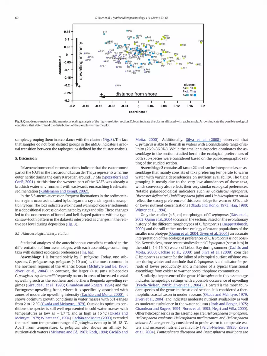
Fig. 8.Q-mode non-metricmultidimensional scaling analysis of the high-resolution section. Colours indicate the cluster affiliatedwith each sample. Arrows indicate the possible ecologicalconditions that determined the distribution of the samples within the plot.

60 G. Auer et al. / Marine Micropaleontology 111 (2014) 53–65

samples, grouping them in accordancewith the clusters (Fig. 8). The factthat samples do not form distinct groups in the nMDS indicates a grad-ual transition between the taphogroups defined by the cluster analysis.

5. Discussion

Palaeoenvironmental reconstructions indicate that the easternmostpart of theNAFB in the area around Laa an der Thaya represents amarineouter neritic during the early Karpatian around 17 Ma (Spezzaferri andĆorić, 2001). At this time the western part of the NAFB was already abrackish water environment with eastwards encroaching freshwatersedimentation (Kuhlemann and Kempf, 2002).

In the 5.5-metre-succession frequent fluctuations in the sedimenta-tion regimeoccur as indicated by both gamma ray andmagnetic suscep-tibility logs. The logs indicate awaxing andwaning of coarser sedimentsin a depositional succession dominated by clays and silts. These changesled to the occurrences of funnel and bell shaped patterns within a typi-cal saw-tooth pattern in the datasets interpreted as changes in the rela-tive sea level during deposition (Fig. 3).

5.1. Palaeoecological interpretation

Statistical analyses of the autochthonous coccoliths resulted in thedifferentiation of four assemblages, with each assemblage containingtaxa with distinct ecological preferences (Fig. 6a):

Assemblage 1 is formed solely by C. pelagicus. Today, one sub-species, C. pelagicus ssp. pelagicus (b10 μm), is the most common inthe northern regions of the Atlantic Ocean (McIntyre and Bé, 1967;Ziveri et al., 2004). In contrast, the larger (N10 μm) sub-speciesC. pelagicus ssp. braarudii frequently occurs in areas of increased coastalupwelling such as the southern and northern Benguela upwelling re-gimes (Giraudeau et al., 1993; Giraudeau and Rogers, 1994) and thePortuguese upwelling front, where it is specifically associated withzones of moderate upwelling intensity (Cachão and Moita, 2000). Itshows optimum growth conditions in water masses with SST-rangesfrom 2 to 12 °C (Okada and McIntyre, 1979). Outside its optimum con-ditions the species is still well represented in cold water masses withtemperatures as low as −1.7 °C and as high as 15 °C (Okada andMcIntyre, 1979;Winter et al., 1994). Cachão andMoita (2000) extendedthe maximum temperature range of C. pelagicus even up to 16–18 °C.Apart from temperature, C. pelagicus also shows an affinity fornutrient-rich waters (McIntyre and Bé, 1967; Roth, 1994; Cachão and

Moita, 2000). Additionally, Silva et al. (2008) observed thatC. pelagicus is able to flourish in waters with a considerable range of sa-linity (26.9–36.0‰). While the smaller subspecies dominates the as-semblage in the section studied herein the ecological preferences ofboth sub-species were considered based on the palaeogeographic set-ting of the studied section.

Assemblage 2 contains all taxa b2% and can be interpreted as an as-semblage that mainly consists of taxa preferring temperate to warmwater with varying dependencies on nutrient availability. The tightgrouping is mostly due to the very low abundances of those taxa,which conversely also reflects their very similar ecological preferences.Notable palaeoecological indicators such as Calcidiscus leptoporus,Discoaster deflandrei, Umbilicosphaera jafari and Umbilicosphaera rotulareflect the strong preference of this assemblage for warmer SSTs and/or lower nutrient concentrations (Okada and Honjo, 1973; Haq, 1980;Winter et al., 1994).

Only the smaller (b5 μm) morphotype of C. leptoporus (Sáez et al.,2003;Quinn et al., 2004) occurs in the section. Based on theevolutionaryhistory of the different morphotypes of C. leptoporus (Knappertsbusch,2000) and the still rather unclear ecology of extant populations of thesmaller morphotype (Quinn et al., 2004; Ziveri et al., 2004) an accurateinterpretation of the ecological preferences of C. leptoporus is not possi-ble. Nevertheless, more recent studies found C. leptoporus (sensu lato) inthe cold (~14–15 °C) waters of Lisbon Bay during summer (Cachão andMoita, 2000; Cachão et al., 2000) and Silva et al. (2008) considerC. leptoporus as a tracer for the influx of subtropical surface offshore wa-ters during winter and conclude that C. leptoporus is an indicator for pe-riods of lower productivity and a member of a typical transitionalassemblage from colder to warmer coccolithophore communities.

Similarly, the presence of the genusHelicosphaera in this assemblageindicates hemipelagic settings with a possible occurrence of upwelling(Perch-Nielsen, 1985b; Ziveri et al., 2004). H. carteri is the most abun-dant species of the genus in the studied section. It is considered a ther-mophilic coastal taxon in modern oceans (Okada and McIntyre, 1979;Ziveri et al., 2004) and indicates moderate nutrient availability as wellas moderate turbulence in the water column (Roth and Berger, 1975;Giraudeau and Rogers, 1994; Flores et al., 1995; Negri and Villa, 2000).Other helicosphaerids in the assemblage are:Helicosphaera ampliaperta,Helicosphaera euphratis, Helicosphaera mediterranea, and Helicosphaerascissura. All are generally considered to prefer warm to temperate wa-ters and increased nutrient availability (Perch-Nielsen, 1985b; Ziveriet al., 2004). Pontosphaera discopora and Pontosphaera multipora are

61G. Auer et al. / Marine Micropaleontology 111 (2014) 53–65

generally described as preferring shelf areas, while being uncommon inopen ocean settings (Perch-Nielsen, 1985b).

B. bigelowii and the closely relatedMicrantholithus vesper (Street andBown, 2000; Bown, 2005) show rather ambiguous ecological prefer-ences (see Aubry, 2013 for extensive discussion). Nevertheless, the spe-cies often bloom in waters of low salinity or even brackish conditions incoastal areas (Peleo-Alampay et al., 1999) and appear to also thriveunder highly eutrophic conditions (Cunha and Shimabukuro, 1997)with a strong influx of terrigenous material (Svabenicka, 1999). Sincethey also occur in the open ocean (Siesser et al., 1992; Peleo-Alampayet al., 1999; Kelly et al., 2003) and especially during times of reducedcompetition and raised nutrient availability (Thierstein et al., 2004),both species cannot be necessarily linked to neritic environments, butrather to periods of high nutrient availability and/or increased environ-mental stress (Wade and Bown, 2006). Based on the palaeogeographicalsetting of the section especially B. bigelowii can thus be regarded as anindicator of environmental stress most likely related to lowered salinityor increased terrigenous influx, caused by an increased proximity to theshore.

Assemblage 3 consists of three taxa (R. pseudoumbilicus,C. mediterranea, S. moriformis) that cannot be easily linked accordingto their preferences for water temperature or nutrient availability.R. pseudoumbilicus is indicative of high nutrient levels with no particularpreferences for water temperature (Lohmann and Carlson, 1981).C. mediterranea occurs in modern temperate to warm waters, withmarked spikes during times between upwelling and downwellingpulses at amoderate distance from the shore (Silva et al., 2008). Similar-ly, while typically being a taxon preferring warm open marine condi-tions, S. moriformis seems to be able to still prosper in shallowercoastal areas and also times of considerable environmental stress(Wade and Bown, 2006). Assemblage 3 can thus be interpreted to re-flect a preference for shallow waters and near-shore environmentswith generally warm to temperate SSTs and a tolerance for varying nu-trient availability; it is considered to be transitional between Assem-blages 2 and 4.

Assemblage 4 includes small and medium-sized reticulofenestrids(R. haqii, R. minuta) as well as C. floridanus and can be interpreted asan assemblage that is indicative of nutrient-rich waters without strongfluctuations in temperature, nutrient availability and surface water tur-bulence. R. minuta in particular is often associated with an increasedavailability of terrigenous nutrients and stable water conditions (Haq,1980; Wade and Bown, 2006). Wei and Wise (1990) considerC. floridanus an indicator for temperate waters. Aubry (1992) suggestedthat the distribution of C. floridanus is not necessarily only an expressionof temperature, but could also reflect high nutrient availability.

Based on the ecological preferences of the considered taxa the clus-ter distribution in the nMDS (Fig. 6b) can be interpreted in the followingway: Coordinate 1 of the nMDS correlates positively to calcareous nan-noplankton taxa able to thrive in waters in a closer proximity to theshore. Coordinate 2 displays a strong negative correlationwith the pref-erences for upwelling conditions. Temperature was defined as a thirdecological factor in the nMDS ranging between coordinate axes 1 and2. The temperature gradient shows a positive correlation with both co-ordinates, placing taxa that prefer cooler water conditions on the lowerleft side and taxa that prefer warmer SSTs on the upper right side. Theseresults indicate that a primary ecological signal is preserved in the au-tochthonous assemblages, despite the fact that certain taxa are likelycontaminated by allochthonous specimens.

The three taphogroups (Fig. 7), with two sub-groups each, reflectsmall-scale changes in palaeoenvironmental conditions:

Taphogroup 1 The high amount of R. minuta in sub-group 1a indicateshigh nutrient levels of terrigenous origin. The highamount of allochthonous taxa in sub-group 1b can becorrelated with high terrigenous influx. Low amountsof the typical open water species C. floridanus support

the assumption that this group occupies a position rela-tively close to the shore. Similarly, the elevated contentof warm water taxa as well as the low content ofC. pelagicus points towards generally warmer SSTs com-pared to the other two groups. In summary, Taphogroup1 is interpreted as being indicative of high terrigenousinflux and a close proximity to the shore.

Taphogroup 2 High amounts of the open ocean species C. floridanus(sub-group 2a) and C. pelagicus (sub-group 2b) indicatethat Taphogroup 2 can be correlated with the greatestdistance from the shore. This is also supported by alow content of warm water and allochthonous taxa.Sub-group 2a was associated with waters showingreducedwater turbulence, based on the higher amountsof C. floridanus. Sub-taphogroup 2b was adapted to up-welling conditions based on the preference ofC. pelagicus for cool nutrient-rich waters.

Taphogroup 3 This group can be interpreted as a transitional group be-tween groups 1 and 2. This assumption is based on highabundances of C. pelagicus that are coupled with moder-ately low to very low abundances of typical warmwatertaxa. C. floridanus is also low in abundance. High con-tents of R. minuta (sub-group 3b) and allochthonoustaxa (sub-group 3a) indicate terrigenous influx andhigh nutrient availability similar to Taphogroup 1.Higher amounts of C. pelagicus in both sub-groups indi-cate colder SSTs comparable to sub-group 2b.

The nMDS plot shows a gradual progression from samples dominat-ed by cool SSTs and upwelling conditions to samples that are dominatedby terrigenous influx and relatively warmer SSTs. The samples do notform separated clusters, but a clear trend is still apparent. Coordinate1 can be thus correlated with the proximity to the shore, while Coordi-nate 2 is negatively correlated with upwelling intensity (Fig. 8).

5.2. Palaeoenvironmental model

The regime under which the studied section was deposited can beconsidered as a marine near-shore environment in the eastern part ofthe NAFB. It is characterised by calcareous nannofossil assemblagesthat point towards cool to temperate SSTs and high nutrient availabilityassociated with terrigenous input and wind-driven upwelling. Geo-chemical data and the largely absent bioturbation indicate anoxic todysoxic bottom water conditions. Previous studies (Spezzaferri andĆorić, 2001; Spezzaferri et al., 2002) further indicated a relative proxim-ity to the shore with water depths not exceeding 200 m based on stud-ied assemblages of benthic foraminifers.

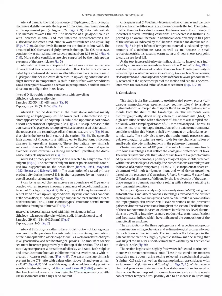
While the overall conditions remain more or less stable during thedeposition of the 940-mm-thick section, the distribution of the definedassemblages and taphogroups and to a lesser degree changes in geo-chemical (see below) and sedimentological proxies clearly point tosmall-scale palaeoenvironmental variations. These data allow a differ-entiation of the section into five intervals (A–E; Fig. 9):

Interval A Shallow neritic fresh water influenced environmentSamples 100–81 (0–212 mm) (Fig. 9)Lithology calcareous silty clayTaphogroups 1a, 1b, 3b (3a) (Fig. 7)

Interval A is the most notable for its low content in sulphur com-pared to all other intervals in the section. The low sulphur contentcoupled with a continuously high carbonate content point towardsmuch better oxygenated bottomwaters compared to the rest of the sec-tion. Higher contents of TOC point to higher fertility levels (Berner andRaiswell, 1984; Kuypers et al., 2002; Twichell et al., 2002).

The nannoplankton assemblages predominantly consist ofC. pelagicus and R. minuta (Figs. 5, 7, 9). Both indicate high primary

A

B

C

D

E

interval

thic

knes

s in

mm

14 16 18 20 22 0.6 0.7 0.8 0.9 0.1 0.3 0.5 2.5 6.3 15.8 39.8 25 35 45 5 15 25 3 6 9 12 15 18 2 6 105 15 25 35 25 35 45

% g

rain

siz

e <

63 μ

m

wt.%

car

bona

te

wt.%

sul

phur

wt.%

TO

C

C/S

-rat

io

% C

occo

lithu

s pe

lagi

cus

% R

etic

ulof

enes

tra

min

uta

% C

yclic

argo

lithu

s flo

ridan

us

Σ %

aut

ocht

hono

us ta

xa <

1%

Σ %

allo

chth

onou

s ta

xa

050

100150

200250

300350

400450

500550

600650

700750

800850

900

Fig. 9. Graphical representation the five described intervals (Interval A–E), as a labelled column. The intervals were additionally plotted in conjunction with key sedimentological, geo-chemical and coccolith abundance data (see Fig. 6) transformed to reflect the thickness of each layer.

62 G. Auer et al. / Marine Micropaleontology 111 (2014) 53–65

productivity under eutrophic conditions. The elevated content of smallreticulofenestrids points to strong influx of terrigenous material and arelative proximity to the shore (Haq, 1980; Aubry, 1992; Flores et al.,1995; Wade and Bown, 2006). This is further supported by highamounts of allochthonous taxa in this interval, indicating increased con-tinental runoff (Fig. 9).

R. minuta is considered to thrive during times of strongly fluctuatingenvironmental conditions (Wade and Bown, 2006), so the intercalationof Taphogroups 1 and 3 is most likely indicative of increased continentalrunoff, explaining changes in the abundance of R. minuta and C. pelagicus.Layers characterised by Taphogroups 1a and 1b and thus higher amountsof R.minuta or allochthonous taxa indicate strong terrigenous influxwithraised nutrient availability possibly coupled with an increased stratifica-tion of water masses (Ćorić and Hohenegger, 2008). This may furtherpoint to repeated input of surface bound fresh water transporting highamounts of reworked Cretaceous and Palaeogene nannoplankton taxa.Hence, the alternation between Taphogroups 1 and 3 can be roughly cor-related with a variability of precipitation in the hinterland. Low levels ofsulphur coupled with continuously high amounts of carbonate and or-ganic carbon (Figs. 4, 9), indicate stable, at least partly oxygenated,bottom-water conditions. Such conditions could also account for the spo-radic bioturbation in the lower part of the high-resolution section (Fig. 3).Berner and Raiswell (1984) point out that levels of organic carbon below1 wt.% are not suitable for a reliable interpretation of the C/S-ratio. How-ever, the general trend of the C/S-ratio in the section still reflects thestrong terrigenous influence in Interval A. Raised levels (2.83–7.41)would at least indicate slightly brackish conditions.

Interval B Transition from fresh water influence to more stable marineconditions

Samples 80–67 (212–292 mm) (Fig. 9)Lithology calcareous silty clayTaphogroups 3b (3a & 1b) (Fig. 7)

Interval B marks the onset of more dysoxic to anoxic bottom waterconditions that are indicated by a slight increase in sulphur (Berner,1981;Maynard, 1982; Berner and Raiswell, 1984). The sediment is fine-ly laminated in this part of the section. The C/S-ratio decreases to typicalmarine conditions pointing towards higher salinity levels and the wan-ing of freshwater influx (Figs. 4, 7, 9). The decrease in bottomwater ox-ygenation coupled with a decrease in influx of terrigenous material andfreshwater, is also expressed by a decrease in small reticulofenestrids(Haq, 1980; Aubry, 1992; Flores et al., 1995; Wade and Bown, 2006).This decrease further points towards a decrease in precipitation in thehinterland or a slight rise in sea level.

This interval shows a dominance of Taphogroup 3. The increase inC. pelagicus may indicate the possible establishment of a more stablewind-driven upwelling cell in the lower part. Lower amounts ofreticulofenestrids as well as allochthonous taxa indicate a decrease ofterrigenous influx (McIntyre and Bé, 1967; Aubry, 1992; Cachão andMoita, 2000; Persico and Villa, 2004). The increase in C. pelagicus goeshand in hand with a small decrease in the overall abundance of taxacompared to Interval A (Figs. 5, 9), reflecting an increase in coolnutrient-richwatermasses that are no longer influenced byfluctuationsin salinity. An ongoing decrease in the amount of allochthonous calcar-eous nannofossils further points towards a decrease in riverine outflow.

The lower part of Interval B marks the first increase in upwellingconditions, which favoured C. pelagicus and primary productivity alsoincreased. Bottom water conditions, however, remained more or lessstable and stagnant. The top of Interval B is characterised by a shortre-establishment of conditions similar to Interval A (samples 70–67;Figs. 7, 9).

Interval C Eutrophic marine conditionsSamples 66–53 (292–431 mm) (Fig. 9)Lithology calcareous silty clayTaphogroups 2a, 2b (3a) (Fig. 7)

63G. Auer et al. / Marine Micropaleontology 111 (2014) 53–65

Interval C marks the first occurrence of Taphogroup 2. C. pelagicusdecreases slightly towards the top and C. floridanus increases stronglyin the uppermost part (sub-group 2a; Figs. 7, 9). Reticulofenestridsalso increase towards the top. The decrease of C. pelagicus coupledwith increases in small and medium-sized reticulofenestrids andC. floridanus indicates a reduction in water turbulence and upwelling(Figs. 5, 7, 9). Sulphur levels fluctuate but are similar to Interval B. Theamount of TOC decreases slightly towards the top. The C/S-ratio staysconsistently at normal marine values, ranging from 2.58 to 1.5 (Figs. 4,7, 9). More stable conditions are also supported by the high speciesevenness of the assemblage (Fig. 5).

Interval C can thus be interpreted to reflect more open marine con-ditions linked to a decrease in freshwater influx. The latter is also indi-cated by a continued decrease in allochthonous taxa. A decrease inC. pelagicus further indicates decreases in upwelling conditions or aslight increase in temperature. A shift in the surface water conditionscould either point towards a decrease in precipitation, a shift in currentdirection, or a slight rise in sea level.

Interval D Eutrophic marine conditions with upwellingLithology calcareous silty claySamples 52–30 (431–684 mm) (Fig. 9)Taphogroups 2b (3b & 3a) (Fig. 7)

Interval D can be described as the most stable interval mainlyconsisting of Taphogroup 2b. The lower part is characterised by ashort appearance of Taphogroup 3b, while the uppermost part showsa short appearance of Taphogroup 3a (Fig. 7). A sharp increase in theabundance of C. pelagicus is coupled with a decrease of all other autoch-thonous taxa in the assemblage. Allochthonous taxa are rare (Fig. 9) anddiversity is the lowest in this part of the section (Fig. 5). The generallyhigh amount of C. pelagicus is still subject to fluctuations, indicatingchanges in upwelling intensity. These fluctuations are similarlyreflected in diversity. While both Shannon–Wiener-index and speciesevenness show lower values during suspected upwelling, the domi-nance index clearly increases (Fig. 5).

Increased primary productivity is also reflected by a high amount ofsulphur (Fig. 9). The content of sulphur further points towards contin-ued low oxygenation on the ocean floor (Berner, 1981; Maynard,1982; Berner and Raiswell, 1984). The assumption of a raised primaryproductivity during Interval D is further supported by an increase inoverall coccolith abundance (Fig. 4).

It can be assumed that an increase in abundance of C. pelagicuscoupled with an increase in overall abundance of coccoliths indicates abloom of C. pelagicus (Figs. 4, 5). Hence, Interval D may be assumed toreflect wind driven upwelling conditions. Dysoxic conditions continueat the oceanfloor, as indicated by high sulphur contents and the absenceof bioturbation. The C/S-ratio exhibits typical values for normal marineconditions throughout Interval D (Fig. 8).

Interval E Decreasing sea level with high terrigenous influxLithology calcareous silty clay with episodic intercalation of sandSamples 29–01 (684–940.5 mm) (Fig. 9)Taphogroups 1–5 (Fig. 7)

Interval E displays a rather different distribution of taphogroupscompared to the previous four intervals. It shows strong fluctuationsof the nannoplankton assemblage as well as well-correlated changesin all geochemical and sedimentological proxies. The amount of coarsersediment increases progressively to the top of the section. The 13 top-most layers represent alternations of silt/clay and sand. Both sulphurand organic carbon fluctuate exhibiting minima synchronous with in-creases in coarser sediment (Figs. 4, 9). The excursions are similarlypresent in the C/S-ratio with values often above 10 and even as highas 21.87 (Figs. 4, 9). Values of this magnitude would normally point to-wards a freshwater zone, but Berner and Raiswell (1984) pointed outthat low levels of organic carbon make the C/S-ratio generally of littleuse in sediments with a high sand content.

C. pelagicus and C. floridanus decrease, while R. minuta and the con-tent of other autochthonous taxa increase towards the top. The contentof allochthonous taxa also increases. The lower content of C. pelagicusindicates reduced upwelling conditions. This decrease is further sup-ported by an overall increase in nannoplankton diversity in this partof the section, as indicated by the Shannon–Wiener and dominance in-dices (Fig. 5). Higher influx of terrigenous material is indicated by highamounts of allochthonous taxa as well as an increase in smallreticulofenestrids. Increases in warm water and ‘near shore’ taxa pointtowards a sea level fall.

At the top, increased freshwater influx, similar to Interval A, is indi-cated by an increase in near-shore taxa such as R. minuta (Haq, 1980)and also the raised amount of allochthonous taxa. Coastal proximity isreflected by a marked increase in accessory taxa such as Sphenolithus,Helicosphaera and Coronosphaera. Spikes of those taxa are predominant-ly recorded in the uppermost part of the section and can thus be corre-lated with the increased influx of coarser sediment (Figs. 5, 7, 9).

6. Conclusions

This study is the first attempt to use integrated proxy records (cal-careous nannoplankton, geochemistry, sedimentology) to analysehigh-resolution outcrop data of upper Burdigalian (Karpatian) sedi-ments from the shelf of the Paratethys Sea. The sediments werebiostratigraphically dated using calcareous nannofossils (NN4). Ahigh-resolution sectionwith a thickness of 940.5mmwas sampled con-tinuouslywith a sampling distance of ~10mmand analysed. The resultsdocument surprisingly rapid fluctuations of the palaeoenvironmentalconditions within this Miocene shelf environment on a decadal to cen-tennial scale. The study also shows that taphonomic processes andpalaeoecological proxies are useful tools for the characterisation ofsmall-scale, short-term fluctuations in the palaeoenvironment.

Cluster analysis and nMDS group the autochthonous nannofossilsinto four assemblages that reflect the ecological preferences of taxa.The results further indicate that,while certain taxa are likely contaminat-ed by reworked specimens, a primary ecological signal is still preservedwithin the assemblages. Generally, the autochthonous assemblages areindicative of a cool to temperate (~14 to 17 °C) eutrophic near-shore en-vironment with high terrigenous input and wind-driven upwelling,based on the presence of C. pelagicus, R. haqii, R. minuta, H. carteri andC. floridanus in all samples. Additionally, the low diversity of the assem-blage suggests a dynamic near-shore setting with a strong variability inenvironmental conditions.

Subsequent Q-mode analyses (cluster analysis and nMDS) using bothautochthonous and allochthonous assemblages revealed three distincttaphogroups with two sub-groups each. While similar in compositionthe taphogroups still reflect small-scale variations of the prevalentpalaeoenvironmental conditions throughout the section. Thedistributionof these taphogroups is based on changes in relative sea level, fluctua-tions in upwelling intensity, primary productivity, water stratificationand freshwater influx, which have influenced the composition of thenannofossil assemblages.

The distribution of the three taphogroups and respective sub-groupsin combinationwith geochemical and sedimentological proxies allowedthe definition of five intervals. The intervals reflect changes in thepalaeoenvironment of a highly dynamic shallow marine setting thatwas subject to small-scale short-term climate variability on a centennialto decadal scale (Fig. 9):

The section begins with slightly freshwater-influenced marine sedi-ments with strong terrigenous input. These initial conditions progresstowards a more open marine setting reflected in geochemical proxies(sulphur, C/S-ratio) as well as the nannoplankton assemblages withan increase in C. floridanus and C. pelagicus (Figs. 7, 9.). While the geo-chemical proxies indicate more or less stable conditions for most ofthe section the nannoplankton assemblages indicate a shift towardscooler water temperatures, possibly due to an increase in upwelling

64 G. Auer et al. / Marine Micropaleontology 111 (2014) 53–65

conditions in the middle part of the section (Figs. 7, 9). Finally, the de-velopment in the uppermost part of the section points towards a de-crease in water depth (Fig. 3). The nannoplankton taphocoenosesfurther support a fall in relative sea-level with elevated amounts of al-lochthonous taxa, as well as higher contents of near shore and stresstaxa, such as R. minuta and Helicosphaera pointing towards a dynamicenvironment with high nutrient levels, most likely of terrestrial originand high terrigenous input (Fig. 9).

Acknowledgements

The authors would like to thank Stjepan Ćorić (Geological Survey ofAustria, Vienna), Patrick Grunert (University of Graz) and Andrea Kern(StateMuseumof NaturalHistory, Stuttgart, Germany) formanyhelpfulcomments and discussions. We also would like to thank Marie-PierreAubry (Rutgers University), for providing key literature. Finally wewould like to thank two anonymous reviewers for their commentsand helpful suggestions, as well as the editor Richard Jordan, for his ed-itorial expertise. Additional thanks go to the participants of the field-course “Paleontological Lab- and Fieldwork 2009” for their help withsampling and the logging of the outcrop and David Strahlhofer (Univer-sity of Graz) for his assistance with sample preparations in the lab. Thisstudy contributes to the Austrian Science Fund (FWF) grants P21414-B16 and P23492-B17.

Appendix A. Supplementary data

Supplementary data to this article can be found online at http://dx.doi.org/10.1016/j.marmicro.2014.06.005.

References

Adamek, J., Brzobohaty, R., Palensky, P., Sikula, J., 2003. The Karpatian in the CarpathianForedeep (Moravia). In: Brzobohaty, R., Cicha, I., Kováč, M., Rögl, F. (Eds.), TheKarpatian — a Lower Miocene Stage of the Central Paratethys. Masaryk University,Brno, pp. 75–89.

Álvarez, M.C., Flores, J.A., Sierro, F.J., Diz, P., Francés, G., Pelejero, C., Grimalt, J.O., 2005. Mil-lennial surface water dynamics in the Ría de Vigo during the last 3000 years as re-vealed by coccoliths and molecular biomarkers. Palaeogeogr. Palaeoclimatol.Palaeoecol. 218 (1–2), 1–13.

Aubry, M.-P., 1984. Handbook of Cenozoic Calcareous Nannoplankton: Book 1.Ortholithae (Discoasters). Micropaleontology Press, New York.

Aubry, M.-P., 1988. Handbook of Cenozoic Calcareous Nannoplankton: Book 2.Ortholithae (Holococcoliths, Ceratoliths, Ortholiths and Others). MicropaleontologyPress, New York.

Aubry, M.-P., 1989. Handbook of Cenozoic Calcareous Nannoplankton: Book 3.Ortholithae (Pentaliths, and Others), Heliolithae (Fasciculiths, Sphenoliths andOthers). Micropaleontology Press, New York.

Aubry, M.-P., 1990. Handbook of Cenozoic Calcareous Nannoplankton: Book 4. Heliolithae(Helicoliths, Cribriliths, Lopadoliths and Others). Micropaleontology Press, New York.

Aubry, M.-P., 1992. Late Paleogene calcareous nannoplankton evolution: a tale of climaticdeterioration. In: Prothero, D.R., Berggren, W.A. (Eds.), Eocene–Oligocene Climaticand Biotic Evolution. Princeton University Press, New Jersey (272-208).

Aubry, M.-P., 1999. Handbook of Cenozoic Calcareous Nannoplankton. Book 5: Heliolithae(Zygoliths and Rhabdoliths). Micropaleontology Press, New York.

Aubry, M.-P., 2013. Cenozoic Coccolithophores: Braarudosphaerales, 1st ed. Micropaleon-tology Press, New York.

Backman, J., Raffi, I., Rio, D., Fornaciari, E., Pälike, H., 2012. Biozonation and biochronologyof Miocene through Pleistocene calcareous nannofossils from low and middle lati-tudes. Newsl. Stratigr. 45 (3), 221–244.

Berner, R.A., 1981. A new geochemical classification of sedimentary environments. J. Sed-iment. Petrol. 51 (2), 359–365.

Berner, R.A., Raiswell, R., 1984. C/S method for distinguishing freshwater from marinesedimentary rocks. Geology 12 (6), 365–368.

Bown, P.R. (Ed.), 1998. Calcareous Nannofossil Biostratigraphy, 1st ed.Chapman & Hall,Cambridge.

Bown, P.R., 2005. Early to mid-Cretaceous calcareous nannoplankton from the northwestPacific Ocean, Leg 198, Shatsky Rise. Proc. Ocean Drill. Program Sci. Results 198, 1–82.

Bown, P.R., Young, J.R., 1998. Techniques. In: Bown, P.R. (Ed.), Calcareous Nannofossil Bio-stratigraphy. Chapman & Hall, Cambridge, pp. 16–28.

Bray, J.R., Curtis, J.T., 1957. An ordination of the upland forest communities of SouthernWisconsin. Ecol. Monogr. 27 (4), 325.

Burnett, J.A., 1998. Upper Cretaceous. In: Bown, P.R. (Ed.), Calcareous Nannofossil Biostra-tigraphy. Chapman & Hall, Cambridge, pp. 132–199.

Cachão, M., Moita, M.T., 2000. Coccolithus pelagicus, a productivity proxy related to mod-erate fronts off Western Iberia. Mar. Micropaleontol. 39 (1–4), 131–155.

Cachão, M., Oliveira, A., Vitorino, J., 2000. Subtropical winter guests, offshore Portugal. J.Nannoplankton Res. 22, 19–26.

Clarke, K.R., 1993. Non-parametric multivariate analyses of changes in community struc-ture. Aust. J. Ecol. 18 (1), 117–143.

Ćorić, S., Hohenegger, J., 2008. Quantitative analyses of calcareous nannoplankton assem-blages from the Baden-Sooss section (MiddleMiocene of Vienna Basin, Austria). Geol.Carpath. Clays 59 (5), 447–460.

Couapel, M.J.J., Beaufort, L., Jones, B.G., Chivas, A.R., 2007. Late Quaternary marginal ma-rine palaeoenvironments of northern Australia as inferred from cluster analysis ofcoccolith assemblages. Mar. Micropaleontol. 65 (3–4), 213–231.

Cunha, A.S., Shimabukuro, S., 1997. Braarudosphaera blooms and anomalous enrichmentsof Nannoconus: evidence from the Turonian south Atlantic, Santos basin, Brazil. J.Nannoplankton Res. 19 (1), 51–55.

Dellmour, R., Harzhauser, M., 2012. The Iváň Canyon, a large Miocene canyon in theAlpine-Carpathian Foredeep. Mar. Pet. Geol. 38 (1), 83–94.

Flores, J.A., Sierro, F.J., Raffi, I., 1995. Evolution of the calcareous nannofossil assemblage asa response to the paleoceanographic changes in the eastern equatorial Pacific Oceanfrom 4 to 2 Ma (Leg 138, Sites 849 and 852). Proc. Ocean Drill. Program Sci. Results138, 163–176.

Fornaciari, E., Rio, D., 1996. Latest Oligocene to early middle Miocene quantitative calcare-ous nannofossil biostratigraphy in the Mediterranean region. Micropaleontology 42(1), 1–36.

Fornaciari, E., Stefano, A.D., Rio, D., Negri, A., 1996. Middle Miocene quantitative calcare-ous nannofossil biostratigraphy in the Mediterranean region. Micropaleontology 42(1), 37–63.

Galović, I., Young, J.R., 2012. Revised taxonomy and stratigraphy of Middle Miocene cal-careous nannofossils of the Paratethys. Micropaleontology 58 (4), 305–334.

Giraudeau, J., Rogers, J., 1994. Phytoplankton biomass and sea-surface temperature esti-mates from sea-bed distribution of nannofossils and planktonic foraminifera in theBenguela upwelling system. Micropaleontology 40 (3), 275–285.

Giraudeau, J., Monteiro, P.M.S., Nikodemus, K., 1993. Distribution andmalformation of liv-ing coccolithophores in the northern Benguela upwelling system off Namibia. Mar.Micropaleontol. 22 (1–2), 93–110.

Gradstein, F., Ogg, J., Schmitz, M., Ogg, G. (Eds.), 2012. The Geologic Time Scale 2012, 1sted.Elsevier, Boston.

Gross, M., Piller, W.E., Scholger, R., Gitter, F., 2011. Biotic and abiotic response topalaeoenvironmental changes at Lake Pannons' western margin (Central Europe,Late Miocene). Palaeogeogr. Palaeoclimatol. Palaeoecol. 312 (1–2), 181–193.

Grunert, P., Harzhauser, M., Rögl, F., Sachsenhofer, R.F., Gratzer, R., Soliman, A., Piller, W.E.,2010a. Oceanographic conditions as a trigger for the formation of an Early Miocene(Aquitanian) Konservat-Lagerstätte in the Central Paratethys Sea. Palaeogeogr.Palaeoclimatol. Palaeoecol. 292 (3–4), 425–442.

Grunert, P., Soliman, A., Ćorić, S., Scholger, R., Harzhauser, M., Piller, W.E., 2010b. Strati-graphic re-evaluation of the stratotype for the regional Ottnangian stage (CentralParatethys, middle Burdigalian). Newsl. Stratigr. 44 (1), 1–16.

Grunert, P., Soliman, A., Ćorić, S., Roetzel, R., Harzhauser, M., Piller, W.E., 2012. Facies de-velopment along the tide-influenced shelf of the Burdigalian Seaway: an examplefrom the Ottnangian stratotype (Early Miocene, middle Burdigalian). Mar.Micropaleontol. 84–85, 14–36.

Hammer, Ø., Harper, D.A.T., 2006. Paleontological Data Analysis, 1st ed. Blackwell Publish-ing Ltd, Oxford.

Hammer, Ø., Harper, D.A.T., Ryan, P.D., 2001. PAST: paleontological statistics softwarepackage for education and data analysis. Palaeontol. Electron. 4 (1), 1–9.

Haq, B.U., 1980. Biogeographic history of Miocene calcareous nannoplankton andpaleoceanography of the Atlantic Ocean. Micropaleontology 26 (4), 414–443.

Hardenbol, J., Thierry, J., Farley, M.B., Jacquin, T., Graciansky, P.-C., Vail, P.R., 1988. Mesozo-ic and Cenozoic sequence chronostratigraphic framework of European basins. In:Graciansky, P.-C., Hardenbol, J., Jacquin, T., Vail, P.R. (Eds.), Mesozoic and Cenozoic Se-quence Stratigraphy of European Basins. SEPM Special Publication, pp. 3–13.

Harzhauser, M., Piller, W.E., 2007. Benchmark data of a changing sea — palaeogeography,palaeobiogeography and events in the Central Paratethys during the Miocene.Palaeogeogr. Palaeoclimatol. Palaeoecol. 253 (1–2), 8–31.

Hohenegger, J., Wagreich, M., 2011. Time calibration of sedimentary sections based on in-solation cycles using combined cross-correlation: dating the gone Badenianstratotype (Middle Miocene, Paratethys, Vienna Basin, Austria) as an example. Int.J. Earth Sci. 101 (1), 339–349.

Kelly, D.C., Norris, R.D., Zachos, J.C., 2003. Deciphering the paleoceanographic significanceof Early Oligocene Braarudosphaera chalks in the South Atlantic. Mar. Micropaleontol.49 (1–2), 49–63.

Kern, A.K., Harzhauser, M., Soliman, A., Piller, W.E., Gross, M., 2012. Precipitation drivendecadal scale decline and recovery of wetlands of Lake Pannon during the Tortonian.Palaeogeogr. Palaeoclimatol. Palaeoecol. 317–318, 1–12.

Kern, A.K., Harzhauser, M., Soliman, A., Piller, W.E., Mandic, O., 2013. High-resolutionanalysis of upper Miocene lake deposits: evidence for the influence of Gleissberg-band solar forcing. Palaeogeogr. Palaeoclimatol. Palaeoecol. 370, 167–183.

Kloosterboer-van Hoeve, M.L., Steenbrink, J., Visscher, H., Brinkhuis, H., 2006. Millennial-scale climatic cycles in the Early Pliocene pollen record of Ptolemais, northern Greece.Palaeogeogr. Palaeoclimatol. Palaeoecol. 229 (4), 321–334.

Knappertsbusch, M., 2000. Morphologic evolution of the coccolithophorid Calcidiscusleptoporus from the Early Miocene to recent. J. Paleontol. 74 (4), 712–730.

Kuhlemann, J., Kempf, O., 2002. Post-Eocene evolution of the North Alpine Foreland Basinand its response to Alpine tectonics. Sediment. Geol. 152 (1–2), 45–78.

Kuypers, M.M.M., Pancost, R.D., Nijenhuis, I.A., Sinninghe Damsté, J.S., 2002. Enhancedproductivity led to increased organic carbon burial in the euxinic North Atlanticbasin during the late Cenomanian oceanic anoxic event. Paleoceanography 17 (4)(3-1-3-13).

65G. Auer et al. / Marine Micropaleontology 111 (2014) 53–65

Lenz, O.K., Wilde, V., Riegel, W., Harms, F.-J., 2010. A 600 ky record of El Niño–SouthernOscillation (ENSO): evidence for persisting teleconnections during theMiddle Eocenegreenhouse climate of Central Europe. Geology 38 (7), 627–630.

Lindqvist, J.K., Lee, D.E., 2009. High-frequency paleoclimate signals from Foulden Maar,Waipiata Volcanic Field, southern New Zealand: an Early Miocene varved lacustrinediatomite deposit. Sediment. Geol. 222 (1–2), 98–110.

Lohmann, G.P., Carlson, J.J., 1981. Oceanographic significance of Pacific Late Miocene cal-careous nannoplankton. Mar. Micropaleontol. 6 (5–6), 553–579.

Martin, R.E., 1999. Taphonomy: A Process Approach. Cambridge University Press,Cambridge.

Martini, E., 1971. Standard Tertiary and Quaternary calcareous nannoplankton zonation.In: Farinacci, A. (Ed.), Proceedings of the Second Planktonic Conference Roma 1970.Edizioni Tecnoscienza, Rome, pp. 739–785.

Maynard, J.B., 1982. Extension of Berner's ‘New geochemical classification of sedimentaryenvironments’ to ancient sediments. J. Sediment. Petrol. 52 (4), 1325–1331.

McIntyre, A., Bé, A.W.H., 1967. Modern coccolithophoridae of the Atlantic Ocean — I.Placoliths and cyrtoliths. Deep-Sea Res. Oceanogr. Abstr. 14 (5), 561–597.

Mertens, K.N.J.M., Lynn, M., Aycard, M., Lin, H.-L., Louwye, S., 2009. Coccolithophores aspalaeoecological indicators for shifts of the ITCZ in the Cariaco Basin during the lateQuaternary. J. Quat. Sci. 24 (2), 159–174.

Meyers, P.A., Arnaboldi, M., 2005. Trans-Mediterranean comparison of geochemicalpaleoproductivity proxies in a mid-Pleistocene interrupted sapropel. Palaeogeogr.Palaeoclimatol. Palaeoecol. 222 (3–4), 313–328.

Mudie, P.J., Marret, F., Aksu, A.E., Hiscott, R.N., Gillespie, H., 2007. Palynological evidencefor climatic change, anthropogenic activity and outflow of Black Sea water duringthe late Pleistocene and Holocene: centennial- to decadal-scale records from theBlack and Marmara Seas. Quat. Int. 167–168, 73–90.

Negri, A., Giunta, S., 2001. Calcareous nannofossil paleoecology in the sapropel S1 of theeastern Ionian sea: paleoceanographic implications. Palaeogeogr. Palaeoclimatol.Palaeoecol. 169 (1–2), 101–112.

Negri, A., Villa, G., 2000. Calcareous nannofossil biostratigraphy, biochronology and paleo-ecology at the Tortonian/Messinian boundary of the Faneromeni section (Crete).Palaeogeogr. Palaeoclimatol. Palaeoecol. 156 (3), 195–209.

Nehyba, S., Petrová, P., 2000. Karpatian sandy deposits in the southern part of theCarpathian Foredeep in Moravia. Bull. Czech Geol. Surv. 75 (1210–3527), 53–66.

Okada, H., Honjo, S., 1973. The distribution of oceanic coccolithophorids in the Pacific.Deep-Sea Res. Oceanogr. Abstr. 20 (4), 355–374.

Okada, H., McIntyre, A., 1979. Seasonal distribution of modern coccolithophores in thewestern North Atlantic Ocean. Mar. Biol. 54 (4) (319–328–328).

Peleo-Alampay, A.M., Mead, G.A., Wei, W., 1999. Unusual Oligocene Braarudosphaera-richlayers of the South Atlantic and their paleoceanographic implications. J. Nannoplank-ton Res. 21 (1), 17–26.

Perch-Nielsen, K., 1985a. Mesozoic calcareous nannofossils. In: Bolli, H.M., Saunders, J.B.,Perch-Nielsen, K. (Eds.), Plankton Stratigraphy Volume 1. Cambridge UniversityPress, Cambridge, pp. 329–426.

Perch-Nielsen, K., 1985b. Cenozoic calcareous nanofossils. In: Bolli, H.M., Saunders, J.B.,Perch-Nielsen, K. (Eds.), Plankton Stratigraphy Volume 1. Cambridge UniversityPress, Cambridge, pp. 427–554.

Persico, D., Villa, G., 2004. Eocene–Oligocene calcareous nannofossils fromMaud Rise andKerguelen Plateau (Antarctica): paleoecological and paleoceanographic implications.Mar. Micropaleontol. 52 (1–4), 153–179.

Piller, W.E., Harzhauser, M., Mandic, O., 2007. Miocene Central Paratethys stratigraphy —current status and future directions. Stratigraphy 4 (2/3), 71–88.

Quinn, P.S., Sáez, A.G., Baumann, K.-H., Steel, B.A., Sprengel, C., Medlin, L.K., 2004.Coccolithophorid biodiversity: evidence from the cosmopolitan species Calcidiscusleptoporus. In: Thierstein, H.R., Young, J.R. (Eds.), Coccolithophores. Springer, Berlin,Heidelberg (299–326–326).

Roetzel, R., Schnabel, W., 2002. Molasse, Waschbergzone, Paläogen und Neogen auf derBöhmischen Masse. 1:200.000 In: Schnabel, W. (Ed.), Legende Und KurzerläuterungDer Geologischen Karte Von Niederösterreich. Geologische Bundesanstalt, Vienna,pp. 23–30.

Roetzel, R., Ćorić, S., Galović, I., Rögl, F., 2007. Early Miocene (Ottnangian) coastal upwell-ing conditions along the southeastern scarp of the BohemianMassif (Parisdorf, LowerAustria, Central Paratethys). Beitr. Paläontol. 30 (2006), 387–413.

Roth, P.H., 1994. Distribution of coccoliths in oceanic sediments. In: Winter, A., Siesser, W.G. (Eds.), Coccolithophores. Cambridge University Press, Cambridge, pp. 199–218.

Roth, P.H., Berger, W.H., 1975. Distribution and dissolution of coccoliths in the south andcentral Pacific. In: Sliter, W.V., Bé, A.W.H., Berger,W.H. (Eds.), Dissolution of Deep-SeaCarbonates. Cushman Foundation Foraminiferal Research, Special Publication, pp.87–113.

Sáez, A.G., Probert, I., Geisen, M., Quinn, P., Young, J.R., Medlin, L.K., 2003. Pseudo-crypticspeciation in coccolithophores. Proc. Natl. Acad. Sci. 100 (12), 7163–7168.

Shannon, C.E., Weaver, W., 1948. A mathematical theory of communication. Bell Syst.Tech. J. 27 (379–423, 623–659).

Siesser, W.G., Bralower, T.J., De Carlo, E.H., 1992. Mid-Tertiary Braarudosphaera-richsediments on the Exmouth Plateau. Proc. Ocean Drill. Program Sci. Results 122,653–663.

Silva, A., Palma, S., Moita, M.T., 2008. Coccolithophores in the upwelling waters ofPortugal: four years of weekly distribution in Lisbon bay. Cont. Shelf Res. 28 (18),2601–2613.

Sokal, R.R., Rohlf, F.J., 1995. Biometry, 3rd ed. W. H. Freeman and Company, New York.Spezzaferri, S., Ćorić, S., 2001. Ecology of Karpatian (Early Miocene) foraminifers and cal-

careous nannoplankton from Laa an der Thaya, Lower Austria: a statistical approach.Geol. Carpath. 52 (6), 361–374.

Spezzaferri, S., Ćorić, S., Hohenegger, J., Rögl, F., 2002. Basin-scale paleobiogeography andpaleoecology: an example from Karpatian (Latest Burdigalian) benthic and plankton-ic foraminifera and calcareous nannofossils from the Central Paratethys. Geobios 35,241–256.

Sprovieri, M., Di Stefano, E., Incarbona, A., Manta, D.S., Pelosi, N., d'Alcalà, M.R., Sprovieri,R., 2012. Centennial- to millennial-scale climate oscillations in the Central–EasternMediterranean Sea between 20,000 and 70,000 years ago: evidence from a high-resolution geochemical and micropaleontological record. Quat. Sci. Rev. 46(C),126–135.

Stax, R., Stein, R., 1995. Data report: organic carbon and carbonate records from Detroitseamount and Patton-Murray seamount: results from sites 882 and 887 (North Pacif-ic Transect). Proc. Ocean Drill. Program Sci. Results 145, 645–655.

Street, C., Bown, P.R., 2000. Palaeobiogeography of Early Cretaceous (Berriasian–Barremian) calcareous nannoplankton. Mar. Micropaleontol. 39 (1–4), 265–291.

Svabenicka, L., 1999. Braarudosphaera-rich sediments in the Turonian of the BohemianCretaceous Basin, Czech Republic. Cretac. Res. 20 (6), 773–782.

Svabenicka, L., Ćorić, S., Andreyeva-Grigorovich, A.S., Halasova, E., Marunteanu, M.,Nagymarosy, A., Oszczypko-Clowes, M., 2003. Central Paratethys Karpatian cal-careous nannofossils. In: Brzobohaty, R., Cicha, I., Kováč, M., Rögl, F. (Eds.), TheKarpatian — a Lower Miocene Stage of the Central Paratethys. Masaryk Universi-ty, Brno, pp. 151–167.

Thierstein, H.R., Cortés, M., Haidar, A.T., 2004. Plankton community behavior on ecologicaland evolutionary time-scales: when models confront evidence. In: Thierstein, H.R.,Young, J.R. (Eds.), Coccolithophores. Springer, Berlin, Heidelberg, pp. 455–479.

Twichell, S.C., Meyers, P.A., Diester-Haass, L., 2002. Significance of high C/N ratios inorganic-carbon-rich Neogene sediments under the Benguela Current upwelling sys-tem. Org. Geochem. 33 (7), 715–722.

Varol, O., 1998. Palaeogene. In: Bown, P.R. (Ed.), Calcareous Nannofossil Biostratigraphy.Chapman & Hall, Cambridge, pp. 200–224.

Wade, B.S., Bown, P.R., 2006. Calcareous nannofossils in extreme environments: theMessinian salinity crisis, Polemi Basin, Cyprus. Palaeogeogr. Palaeoclimatol.Palaeoecol. 233 (3–4), 271–286.

Ward Jr., J.H., 1963. Hierarchical grouping to optimize an objective function. J. Am. Stat.Assoc. 58 (301), 236–244.

Wei, W.,Wise Jr., S.W., 1990. Biogeographic gradients of middle Eocene–Oligocene calcar-eous nannoplankton in the South Atlantic Ocean. Palaeogeogr. Palaeoclimatol.Palaeoecol. 79 (1–2), 29–61.

Winter, A., Jordan, R., Roth, P.H., 1994. Biogeography of living coccolithophores in oceanwaters. In: Winter, A., Siesser, W.G. (Eds.), Coccolithophores. Cambridge UniversityPress, Cambridge, pp. 13–37.

Young, J.R., 1998. Neogene. In: Bown, P.R. (Ed.), Calcareous Nannofossil Biostratigraphy.Chapman & Hall, Cambridge, pp. 225–265.

Young, J.R., Bown, P.R., Lees, J.A. (Eds.), 2013. Nannotax Website. International Nanno-plankton Association (URL http://nannotax.org (accessed: 14. March 2013)).

Ziveri, P., Baumann, K.-H., Böckel, B., Bollmann, J., Young, J.R., 2004. Biogeography of se-lected Holocene coccoliths in the Atlantic Ocean. In: Thierstein, H.R., Young, J.R.(Eds.), Coccolithophores: From Molecular Processes to Global Impact. Springer,Berlin, Heidelberg, pp. 403–428.