High-Redshift Quasars Found in Sloan Digital Sky Survey Commissioning Data. V. Hobby-Eberly Telescope Observations

arX

iv:a

stro

-ph/

0012

083v

1 4

Dec

200

0

To Appear in The Astronomical Journal

High-Redshift Quasars Found in Sloan Digital Sky Survey Commissioning

Data V. Hobby-Eberly Telescope Observations 1,2

Donald P. Schneider3, Xiaohui Fan4,5, Michael A. Strauss4, James E. Gunn4,

Gordon T. Richards3, Gary J. Hill6, Phillip J. MacQueen6, Lawrence W. Ramsey3,

Mark T. Adams6, John A. Booth6, Grant M. Hill6, G.R. Knapp4, Robert H. Lupton4,

David H. Saxe5, Matthew Shetrone6, Joseph R. Tufts6, Daniel E. Vanden Berk8, Marsha J. Wolf6,

Donald G. York7, John E. Anderson, Jr.8, Scott F. Anderson9, Neta A. Bahcall4, J. Brinkmann10,

Robert Brunner11, Istvan Csabai12,13, Masataka Fukugita14,5, G.S. Hennessy15, Zeljko Ivezic4,

Donald Q. Lamb7, Jeffrey A. Munn16, and Aniruddha R. Thakar12

email addresses: [email protected], [email protected], [email protected]

1Based on observations obtained with the Sloan Digital Sky Survey, which is owned and operated by the

Astrophysical Research Consortium.

2Based on observations obtained with the Hobby-Eberly Telescope, which is a joint project of the University of

Texas at Austin, the Pennsylvania State University, Stanford University, Ludwig-Maximillians-Universitat Munchen,

and Georg-August-Universitat Gottingen.

3Department of Astronomy and Astrophysics, The Pennsylvania State University, University Park, PA 16802.

4Princeton University Observatory, Princeton, NJ 08544.

5The Institute for Advanced Study, Princeton, NJ 08540.

6Department of Astronomy, McDonald Observatory, University of Texas, Austin, TX 78712.

7Astronomy and Astrophysics Center, University of Chicago, 5640 South Ellis Avenue, Chicago, IL 60637.

8Fermi National Accelerator Laboratory, P.O. Box 500, Batavia, IL 60510.

9University of Washington, Department of Astronomy, Box 351580, Seattle, WA 98195.

10Apache Point Observatory, P.O. Box 59, Sunspot, NM 88349-0059.

11Astronomy Department, California Institute of Technology, Pasadena, CA 91125.

12Department of Physics and Astronomy, Johns Hopkins University, 3701 University Drive, Baltimore, MD 21218.

13Department of Physics of Complex Systems, Eotvos University, Pazmay Peter setany 1/A, H-1117, Budapest,

Hungary.

14Institute for Cosmic Ray Research, University of Tokyo, Midori, Tanashi, Tokyo 188-8588, Japan

15US Naval Observatory, 3450 Massachusetts Avenue NW, Washington, DC 20392-5420.

16US Naval Observatory, Flagstaff Station, P.O. Box 1149, Flagstaff, AZ 86002-1149.

– 2 –

ABSTRACT

We report the discovery of 27 quasars with redshifts between 3.58 and 4.49. The

objects were identified as high-redshift candidates based on their colors in Sloan Digital

Sky Survey commissioning data. The redshifts were confirmed with low resolution

spectra obtained at the Hobby-Eberly Telescope. The quasars’ i∗ magnitudes range

from 18.55 to 20.97. Nearly 60% of the quasar candidates observed are confirmed

spectroscopically as quasars. Two of the objects are Broad Absorption Line quasars,

and several other quasars appear to have narrow associated absorption features.

Subject headings: cosmology: early universe — quasars:individual

1. Introduction

The Sloan Digital Sky Survey (SDSS; York et al. 2000) has proven to be a rich source of

high-redshift (z ≥ 3.5) quasars; to date, 86 high-redshift quasars have been published by the SDSS,

including four that have redshifts larger than 4.95 (Fan et al. 1999, Paper I; 2000a, Paper II;

2000b; 2001a, Paper III; Schneider et al. 2000a,b; Zheng et al. 2000). In this paper we report the

discovery of 27 quasars at 3.5 < z < 4.5 taken from SDSS commissioning data along the Celestial

Equator. High-redshift quasar candidates were identified using a multicolor selection technique

(e.g., Warren, Hewett, and Osmer 1994). Low-resolution spectra of the candidates were obtained

with the Hobby-Eberly Telescope (HET; Ramsey et al. 1998, Hill 2000) during its first year

of science operations. The data were acquired as part of our investigation of the high-redshift

quasar luminosity function using SDSS data. Eight of the objects discussed in this paper (many

of the brighter ones located in the Southern Galactic sky) form part of the complete sample of

high-redshift quasars discussed in Paper III and by Fan et al. (2001b, Paper IV). The remaining

quasars do not form a complete sample, but are presented at this time so the community can have

rapid access to the sources, several of which have interesting absorption features.

The SDSS and HET observations are described in §2, the properties of the quasars presented

in §3, and a brief discussion appears in §4. Throughout this paper we will adopt the cosmological

model with H0 = 50 km s−1 Mpc−1, Ω0 = 1.0, and Λ = 0.0.

2. Observations

– 3 –

2.1. Sloan Digital Sky Survey

The Sloan Digital Sky Survey uses a CCD camera (Gunn et al. 1998) on a dedicated

2.5-m telescope (Siegmund et al. 2001) at Apache Point Observatory, New Mexico, to obtain

images in five broad optical bands over 10,000 deg2 of the high Galactic latitude sky centered

approximately on the North Galactic Pole. The five filters (designated u′, g′, r′, i′, and z′) cover

the entire wavelength range of the CCD response (Fukugita et al. 1996; Paper III). Photometric

calibration is provided by simultaneous observations with a 20-inch telescope at the same site. The

survey data processing software measures the properties of each detected object in the imaging

data, and determines and applies astrometric and photometric calibrations (Pier et al. 2001;

Lupton et al. 2001).

The high photometric accuracy of the SDSS images and the information provided by the

z′ filter (central wavelength of 8873 A, see Paper III) make the SDSS data an excellent source

for identification of high-redshift quasar candidates. The SDSS high-redshift quasar selection

efficiency (number of quasars divided by the number of quasar candidates) is approximately

60–70% (e.g., Papers I, II, and III) for sources with i∗ < 20.0, which is a much higher value than

that achieved in previous investigations in this field.

We have started a survey of faint, high-redshift quasars using the SDSS imaging data. This

investigation uses a multicolor selection technique to identify suitable candidates; the locations of

z > 3.5 quasars in the multidimensional SDSS color space are well separated from the stellar locus

(see Fan 1999; Papers I and II). A detailed discussion of the selection criteria can be found in

Paper III and references therein. For the quasars in this paper, all having redshifts less than 4.5,

the (g∗ − r∗, r∗ − i∗) diagram is the key to separating the quasars from the stellar locus. In this

study the candidates must have an i∗ magnitude brighter than 21.0; this is one magnitude fainter

than the limit imposed in Papers I and II, and that of the complete sample in Papers III and IV.

We are currently assembling a sample of quasars down to a magnitude limit i∗ = 21 to investigate

the z > 3.5 quasar luminosity function luminosities considerably fainter than that reached in

Paper IV.

The quasars presented here were identified from four different SDSS scans along

the Celestial Equator (observation dates in parentheses): 94 (1998 September 19),

125 (1998 September 25), 745 (1999 March 20), and 756 (1999 March 22). All of the data

were taken under photometric conditions, and the typical seeing was 1.5′′. The total area covered

is approximately 500 square degrees.

Notes on SDSS nomenclature: The source name format is SDSSp Jhhmmss.ss+ddmmss.s,

where the coordinate equinox is J2000, and the “p” refers to the preliminary nature of the

astrometry. The reported magnitudes are based on a preliminary photometric calibration; to

indicate this, the filters have an asterisk instead of a prime superscript. The estimated astrometric

accuracies in each coordinate are 0.15′′ and the calibration of the photometric measurements is

accurate to 0.04 magnitudes in the g′, r′, and i′ filters and 0.06 magnitudes in the u′ and z′ bands.

– 4 –

Throughout the text, object names will be abbreviated as SDSShhmm+ddmm.

2.2. Spectroscopy of Quasar Candidates

Spectra of 50 SDSS high-redshift quasar candidates were obtained with the HET’s

Marcario Low Resolution Spectrograph (LRS; Hill et al. 1998a,b; Cobos Duenas et al. 1998;

Schneider et al. 2000b) between October 1999 and June 2000. The LRS is mounted in the

Prime Focus Instrument Package, which rides on the HET tracker. The dispersive element

was a 300 line mm−1 grism blazed at 5500 A. An OG515 blocking filter was installed to permit

calibration of the spectra beyond 8000 A. The detector is a thinned, antireflection-coated

3072 × 1024 Ford Aerospace CCD, and was binned 2 × 2 during readout; this produced an image

scale of 0.50′′ pixel−1 and a dispersion of ≈ 4.5 A pixel−1. The spectra covered the range from

5100–10,200 A at a resolution of approximately 20 A.

The wavelength calibration was provided by Ne, Cd, and Ar comparison lamps; a cubic fit to

the lines produced an rms error of less than 1 A. The relative flux calibration and atmospheric

absorption band corrections were performed by observations of spectrophotometric standards,

usually the primary spectrophotometric standards of Oke & Gunn (1983). The objects were

observed under a wide range of conditions; the FWHM of the spectra ranged from slightly

under 2′′ to over 4′′. The exposure times varied from 566 s to 1800 s, with a median of 800 s.

Absolute spectrophotometric calibration was performed by scaling each spectrum so that the r∗

and i∗ magnitudes synthesized from the spectra matched the SDSS photometric measurements;

this scaling used the new SDSS response curves of Paper III.

Of the 50 objects observed, the spectra of two had essentially no signal (weather related),

13 had featureless spectra (usually low S/N, but of sufficient quality to rule out a typical quasar

Lyman α emission line), one was a faint carbon star (see Margon et al. 2001), two were strong,

narrow emission line objects at redshifts of a few tenths, three were E-type galaxies at redshifts

between 0.4 and 0.7, three were E+A galaxies at redshifts of ≈ 0.4 (in these objects, the Balmer

jump produces SDSS colors that mimic the Lyman α emission line/forest boundary), and 28

were quasars with redshifts between 3.58 and 4.49. One of the quasars, the brighter member of

a z = 4.25 pair, was described by Schneider et al. 2000a. This efficiency (28 of 48, or 58%) is

comparable to previous SDSS studies.

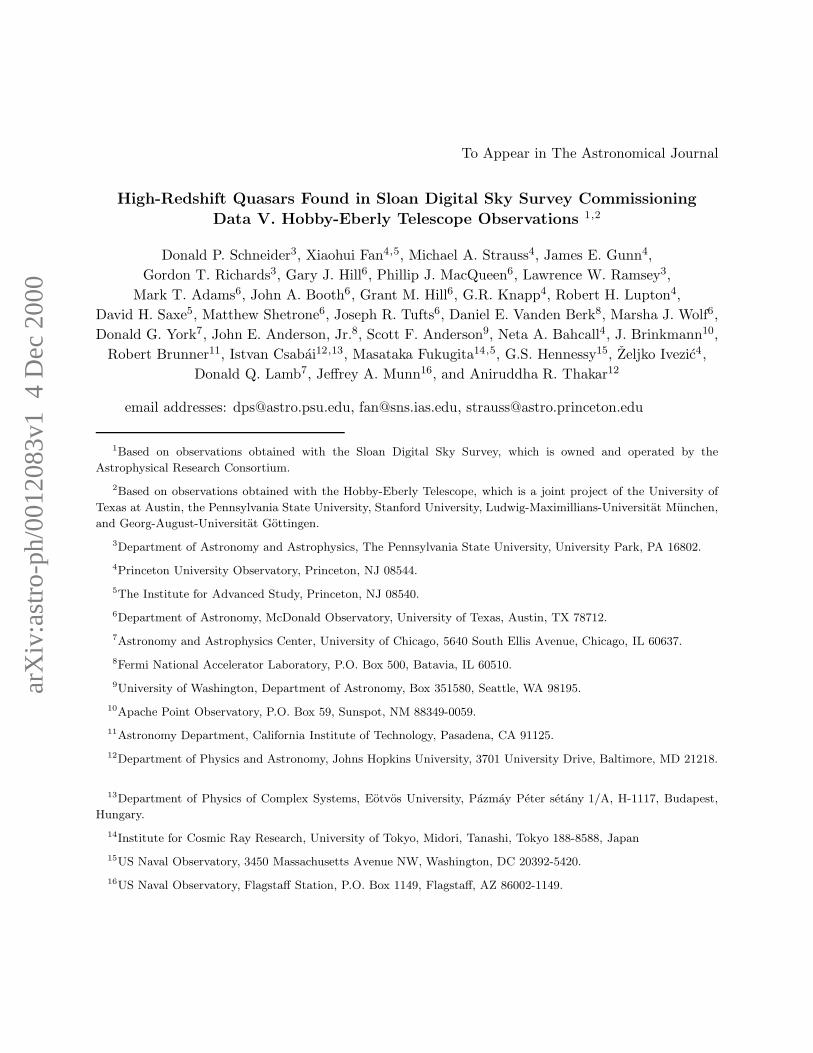
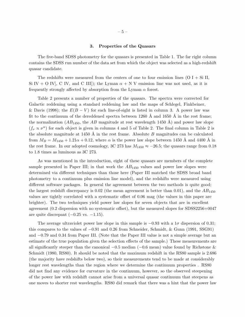
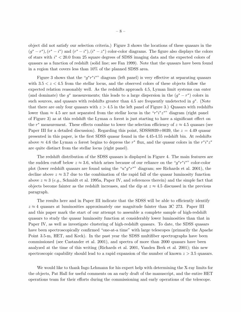
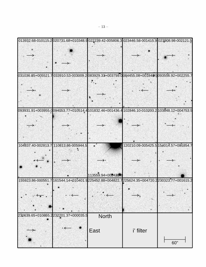
Finding charts for the 27 new quasars are given in Figure 1; each panel is the SDSS i′ image

of the field. (The finding chart for the z = 4.25 quasar mentioned in the previous paragraph can

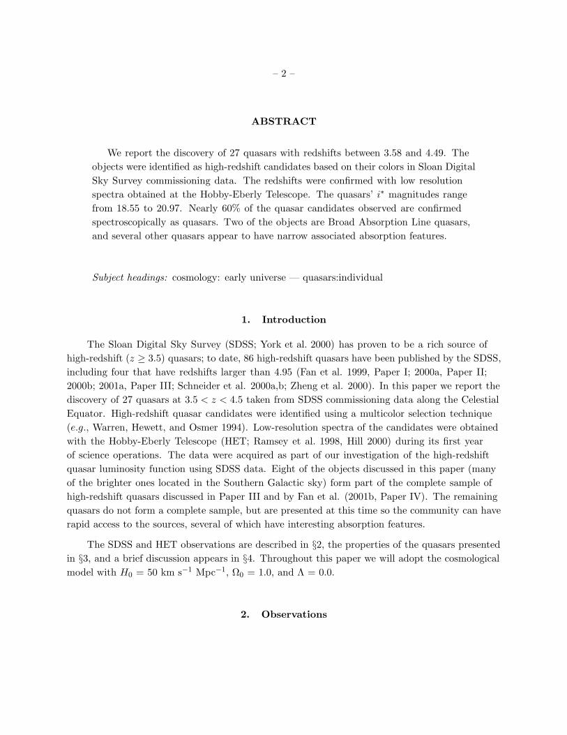
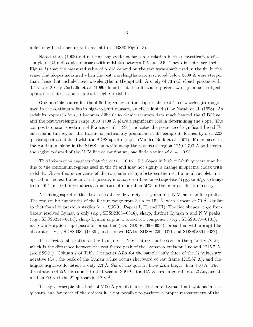
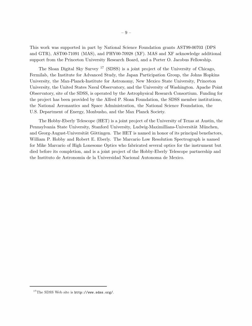
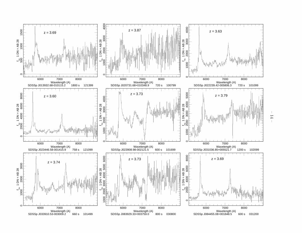
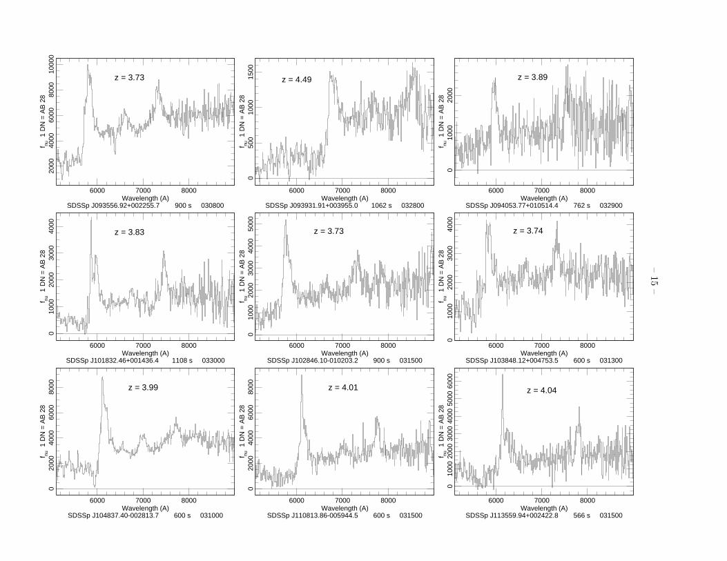
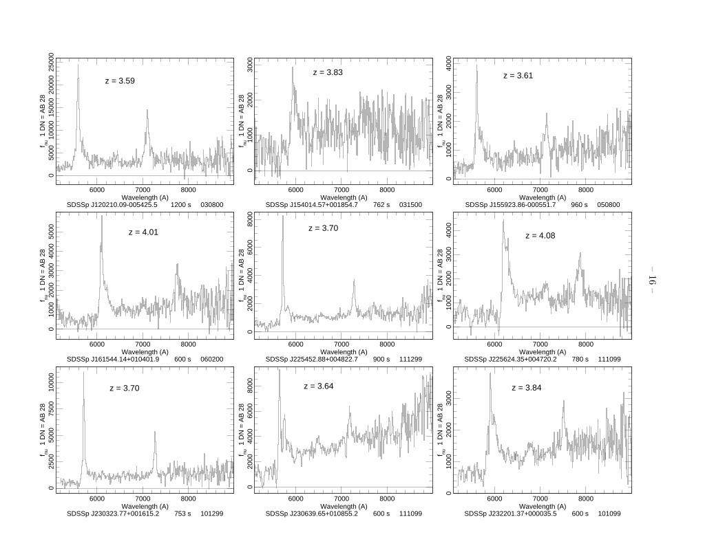
be found in Schneider et al. 2000a.) The flux and wavelength calibrated spectra of the objects

are presented in Figure 2, where the data have been rebinned at 8 A pixel−1. We do not show

the data beyond 9000 A as the signal-to-noise ratio in this region is low for the vast majority of

the objects. Two of the spectra (SDSS0239−0021 and SDSS0839+0037) display prominent BAL

features, and the sample contains a wide variety of Lyman α emission line profiles.

– 5 –

3. Properties of the Quasars

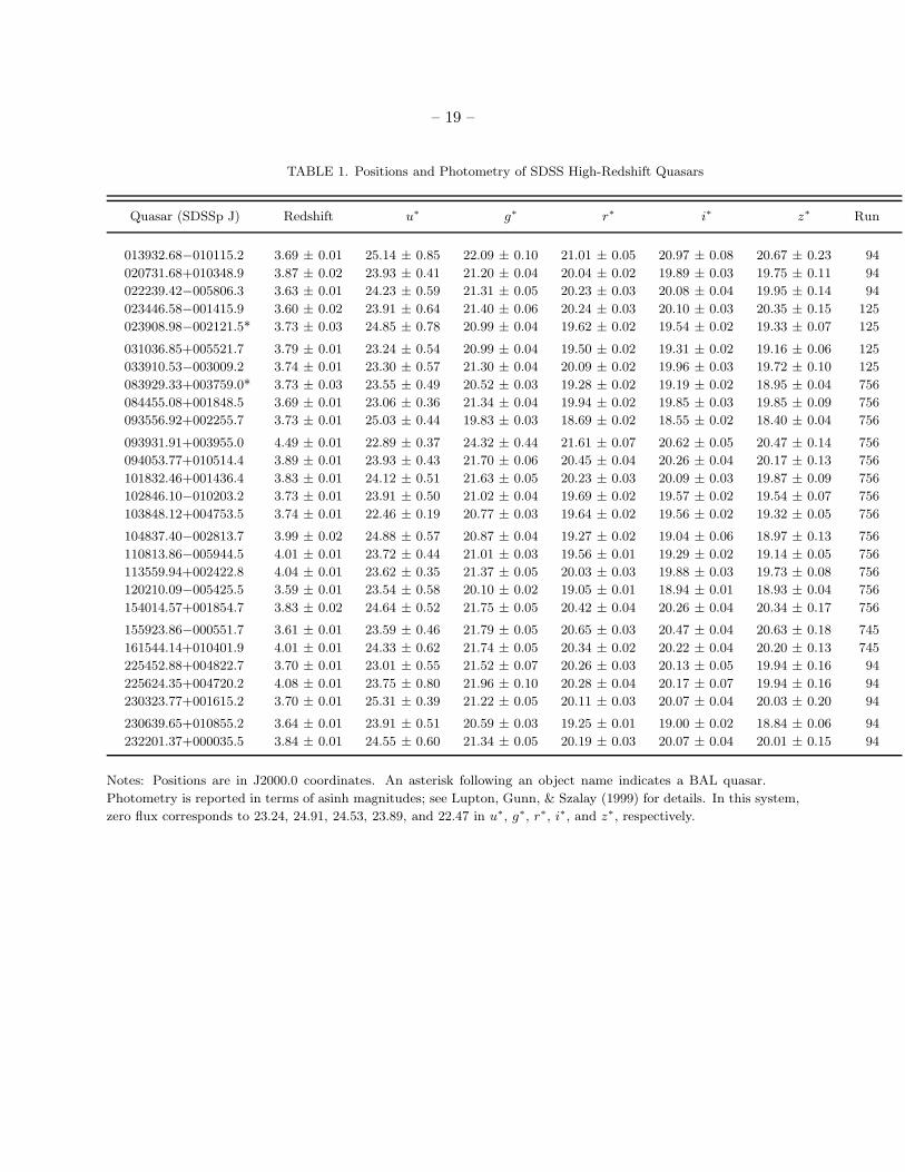
The five-band SDSS photometry for the quasars is presented in Table 1. The far right column

contains the SDSS run number of the data set from which the object was selected as a high-redshift

quasar candidate.

The redshifts were measured from the centers of one to four emission lines (O I + Si II,

Si IV + O IV], C IV, and C III]); the Lyman α + N V emission line was not used, as it is

frequently strongly affected by absorption from the Lyman α forest.

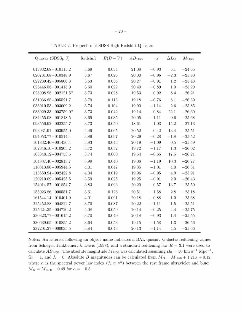
Table 2 presents a number of properties of the quasars. The spectra were corrected for

Galactic reddening using a standard reddening law and the maps of Schlegel, Finkbeiner,

& Davis (1998); the E(B − V ) for each line-of-sight is listed in column 3. A power law was

fit to the continuum of the dereddened spectra between 1260 A and 1650 A in the rest frame;

the normalization (AB1450, the AB magnitude at rest wavelength 1450 A) and power law slope

(fν ∝ να) for each object is given in columns 4 and 5 of Table 2. The final column in Table 2 is

the absolute magnitude at 1450 A in the rest frame. Absolute B magnitudes can be calculated

from MB = M1450 + 1.21α + 0.12, where α is the power law slope between 1450 A and 4400 A in

the rest frame. In our adopted cosmology, 3C 273 has M1450 ≈ −26.5; the quasars range from 0.18

to 1.8 times as luminous as 3C 273.

As was mentioned in the introduction, eight of these quasars are members of the complete

sample presented in Paper III; in that work the AB1450 values and power law slopes were

determined via different techniques than those here (Paper III matched the SDSS broad band

photometry to a continuum plus emission line model), and the redshifts were measured using

different software packages. In general the agreement between the two methods is quite good;

the largest redshift discrepancy is 0.02 (the mean agreement is better than 0.01), and the AB1450

values are tightly correlated with a systematic offset of 0.06 mag (the values in this paper are

brighter). The two techniques yield power law slopes for seven objects that are in excellent

agreement (0.2 dispersion with no systematic offset), but the measured slopes for SDSS2256+0047

are quite discrepant (−0.25 vs. −1.15).

The average ultraviolet power law slope in this sample is −0.93 with a 1σ dispersion of 0.31;

this compares to the values of −0.91 and 0.26 from Schneider, Schmidt, & Gunn (1991, SSG91)

and −0.79 and 0.34 from Paper III. (Note that the Paper III value is not a simple average but an

estimate of the true population given the selection effects of the sample.) These measurements are

all significantly steeper than the canonical −0.5 median (−0.6 mean) value found by Richstone &

Schmidt (1980, RS80). It should be noted that the maximum redshift in the RS80 sample is 2.686

(the majority have redshifts below two), so their measurements tend to be made at considerably

longer rest wavelengths than the region where we determine the continuum properties . RS80

did not find any evidence for curvature in the continuum, however, so the observed steepening

of the power law with redshift cannot arise from a universal quasar continuum that steepens as

one moves to shorter rest wavelengths. RS80 did remark that there was a hint that the power law

– 6 –

index may be steepening with redshift (see RS80 Figure 8).

Natali et al. (1998) did not find any evidence for a α-z relation in their investigation of a

sample of 62 radio-quiet quasars with redshifts between 0.5 and 2.5. They did note (see their

Figure 3) that the measured value of α did depend on the rest wavelength used in the fit, in the

sense that slopes measured when the rest wavelengths were restricted below 3000 A were steeper

than those that included rest wavelengths in the optical. A study of 73 radio-loud quasars with

0.4 < z < 2.8 by Carballo et al. (1999) found that the ultraviolet power law slope in such objects

appears to flatten as one moves to higher redshift.

One possible source for the differing values of the slope is the restricted wavelength range

used in the continuum fits in high-redshift quasars, an effect hinted at by Natali et al. (1998). As

redshifts approach four, it becomes difficult to obtain accurate data much beyond the C IV line,

and the rest wavelength range 1600–1700 A plays a significant role in determining the slope. The

composite quasar spectrum of Francis et al. (1991) indicates the presence of significant broad Fe

emission in this region; this feature is particularly prominent in the composite formed by over 2200

quasar spectra obtained with the SDSS spectrographs (Vanden Berk et al. 2001). If one measures

the continuum slope in the SDSS composite using the rest frame region 1250–1700 A and treats

the region redward of the C IV line as continuum, one finds a value of α = −0.93.

This information suggests that the α ≈ −1.0 to −0.8 slopes in high redshift quasars may be

due to the continuum regions used in the fit and may not signify a change in spectral index with

redshift. Given this uncertainty of the continuum shape between the rest frame ultraviolet and

optical in the rest frame in z ≈ 4 quasars, it is not clear how to extrapolate M1450 to MB ; a change

from −0.5 to −0.9 in α induces an increase of more than 50% in the inferred blue luminosity!

A striking aspect of this data set is the wide variety of Lyman α + N V emission line profiles.

The rest equivalent widths of the feature range from 30 A to 151 A, with a mean of 70 A, similar

to that found in previous studies (e.g., SSG91, Papers I, II, and III). The line shapes range from

barely resolved Lyman α only (e.g., SDSS2303+0016), sharp, distinct Lyman α and N V peaks

(e.g., SDSS0234−0014), sharp Lyman α plus a broad red component (e.g., SDSS0139−0101),

narrow absorption superposed on broad line (e.g., SDSS0339−0030), broad line with abrupt blue

absorption (e.g., SDSS0939+0039), and the two BALs (SDSS0239−0021 and SDSS0839+0037).

The effect of absorption of the Lyman α + N V feature can be seen in the quantity ∆Lα,

which is the difference between the rest frame peak of the Lyman α emission line and 1215.7 A

(see SSG91). Column 7 of Table 2 presents ∆Lα for the sample; only three of the 27 values are

negative (i.e., the peak of the Lyman α line occurs shortward of rest frame 1215.67 A), and the

largest negative deviation is only 2.3 A. Six of the quasars have ∆Lα larger than +10 A. The

distribution of ∆Lα is similar to that seen in SSG91; the BALs have large values of ∆Lα, and the

median ∆Lα of the 27 quasars is +2.8 A.

The spectroscopic blue limit of 5100 A prohibits investigation of Lyman limit systems in these

quasars, and for most of the objects it is not possible to perform a proper measurement of the

– 7 –

continuum depression (DA) produced by the Lyman α forest. Three objects, (SDSS1135+0024,

SDSS2256+0047, and SDSS2306+0108), have strong absorption features that have redshifts

of ≈ 3.6 if they are damped Lyman α lines.

One of the quasars, SDSS0844+0018 (z = 3.69), is radio-loud; it has an observed 20 cm flux

density of 6.05 mJy in the FIRST (Becker, White & Helfand 1995) survey. The other 26 quasars

are not detected at the 1 mJy level and are therefore radio-quiet, as are the vast majority of

optically selected z > 3 quasars (Schneider et al. 1992; Schmidt et al. 1995b; Stern et al. 2000).

None of the quasars are found in the ROSAT Bright Survey Catalog (Schwope et al. 2000), which

has a flux limit of 2.4 × 10−12 erg cm−2 s−1 in the 0.5 to 2.0 keV band; this is not surprising given

that except for a few exceptional sources (e.g., blazars), high-redshift quasars have X-ray fluxes

well below the catalog limit (Kaspi, Brandt, & Schneider 2000; Brandt et al. 2001).

Notes on Individual Objects

SDSSp J023446.58−001415.9 (z = 3.60): The Lyman α, N V, and C IV lines all have a very

sharp core and broad wings.

SDSSp J023908.98−002121.5 (z = 3.73): A BAL with a number of quite impressive absorption

troughs; the C IV feature nearly reaches zero even at this low spectral resolution.

SDSSp J031036.85+005521.7 (z = 3.79): The C IV emission line is split into two sections by a

very deep, narrow absorption feature that appears to be centered slightly to the red of the center

of the emission line. The center of this absorption nearly reaches zero flux density even at this

spectral resolution.

SDSSp J033910.53−003009.2 (z = 3.74): Narrow absorption features are present on the blue

wing of the C IV emission line and in the Lyman α + N V emission line; the absorptions are

probably produced by intrinsic C IV and N V, respectively.

SDSSp J083929.33+003759.0 (z = 3.73): A BAL with several strong BAL troughs.

SDSSp J230323.77+001615.2 (z = 3.70): The spectrum shows strong, barely resolved

Lyman α + N V and C IV lines.

SDSSp J230639.65+010855.2 (z = 3.64): This is probably another example of a quasar with

associated N V and C IV absorpton.

4. Discussion

The results in this paper bring the total number of published z > 3.5 quasars identified by

the SDSS to 113; 23 have redshifts larger than 4.4. (Six of the 113 objects were previously known,

but the SDSS quasar selection algorithm identified them as high-redshift quasar candidates. We

will include the six objects in the discussion and figures that follow. We do not include the fainter

quasar of the z = 4.25 pair serendipitously found by the SDSS [Schneider et al. 2000a] as this

– 8 –

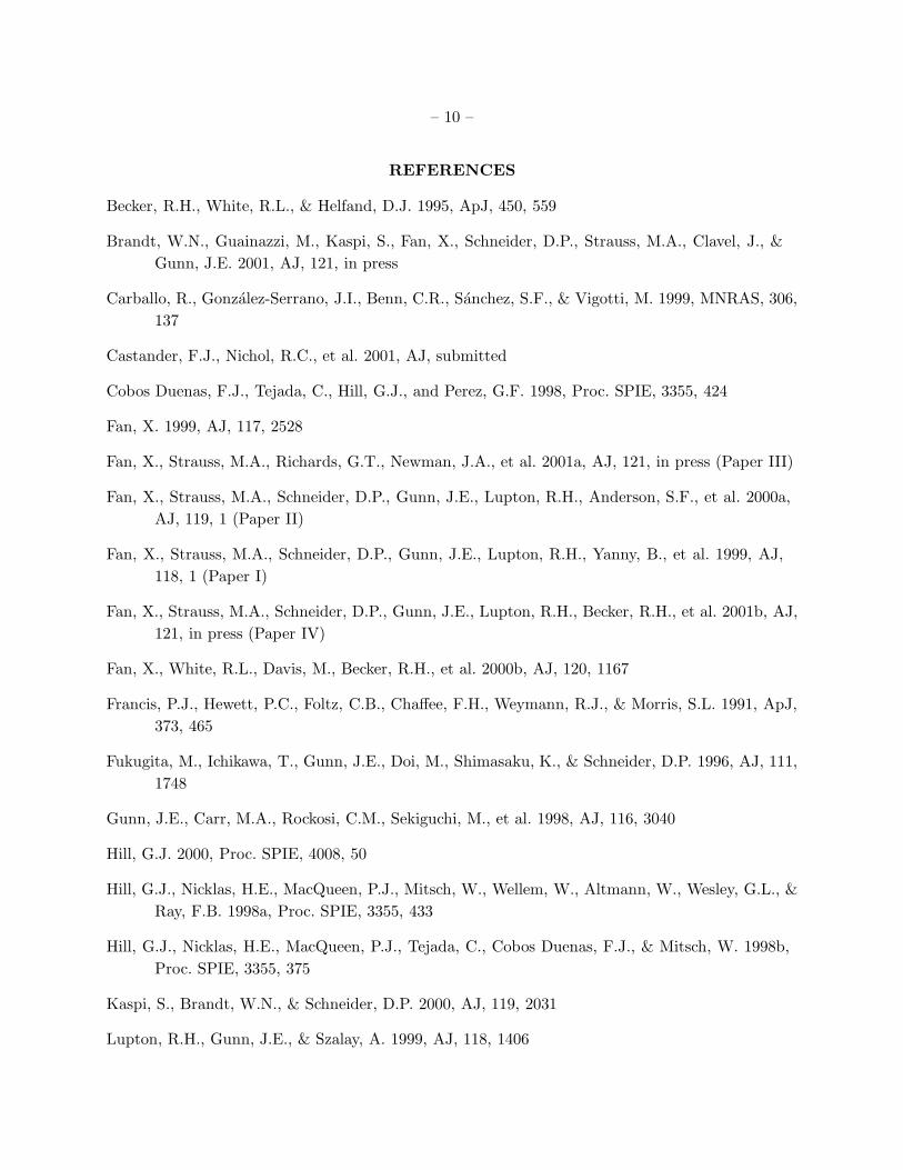
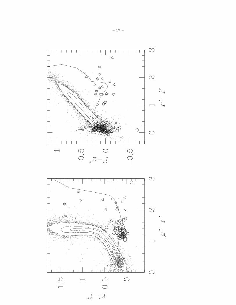
object did not satisfy our selection criteria.) Figure 3 shows the locations of these quasars in the

(g∗ − r∗), (r∗ − i∗) and (r∗ − i∗), (i∗ − z∗) color-color diagrams. The figure also displays the colors

of stars with i∗ < 20.0 from 25 square degrees of SDSS imaging data and the expected colors of

quasars as a function of redshift (solid line; see Fan 1999). Note that the quasars have been found

in a region that covers less than 10% of the planned SDSS area.

Figure 3 shows that the “g∗r∗i∗” diagram (left panel) is very effective at separating quasars

with 3.5 < z < 4.5 from the stellar locus, and the observed colors of these objects follow the

expected relation reasonably well. As the redshifts approach 4.5, Lyman limit systems can enter

(and dominate) the g∗ measurements; this leads to a large dispersion in the (g∗ − r∗) colors in

such sources, and quasars with redshifts greater than 4.5 are frequently undetected in g∗. (Note

that there are only four quasars with z > 4.5 in the left panel of Figure 3.) Quasars with redshifts

lower than ≈ 4.5 are not separated from the stellar locus in the “r∗i∗z∗” diagram (right panel

of Figure 3) as at this redshift the Lyman α forest is just starting to have a significant effect on

the r∗ measurement. These effects combine to lower the selection efficiency of z ≈ 4.5 quasars (see

Paper III for a detailed discussion). Regarding this point, SDSS0939+0039, the z = 4.49 quasar

presented in this paper, is the first SDSS quasar found in the 4.45-4.55 redshift bin. At redshifts

above ≈ 4.6 the Lyman α forest begins to depress the r∗ flux, and the quasar colors in the r∗i∗z∗

are quite distinct from the stellar locus (right panel).

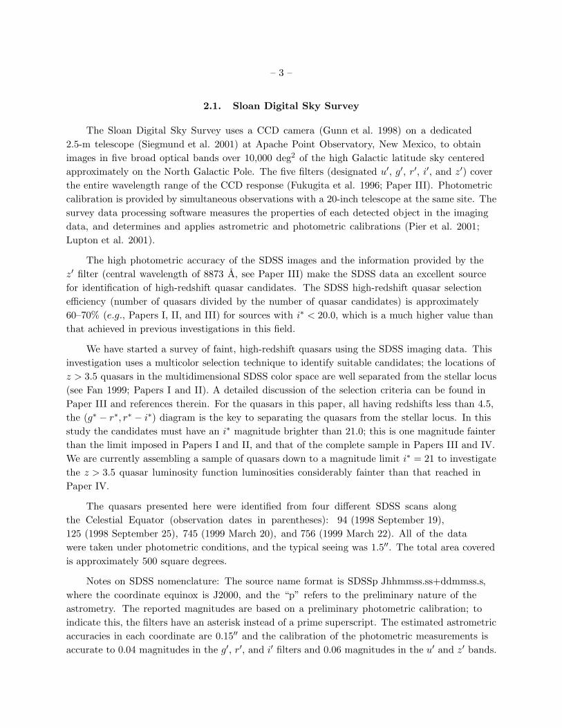
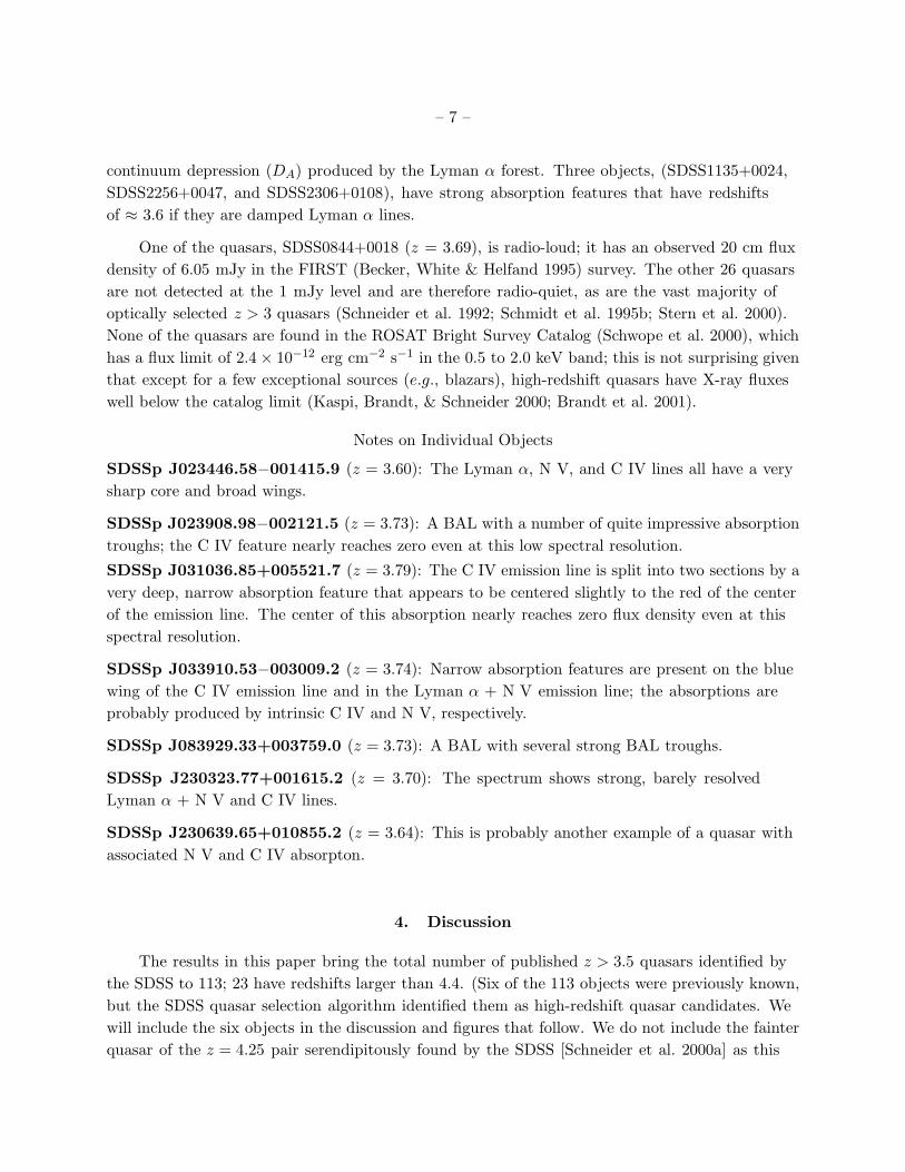
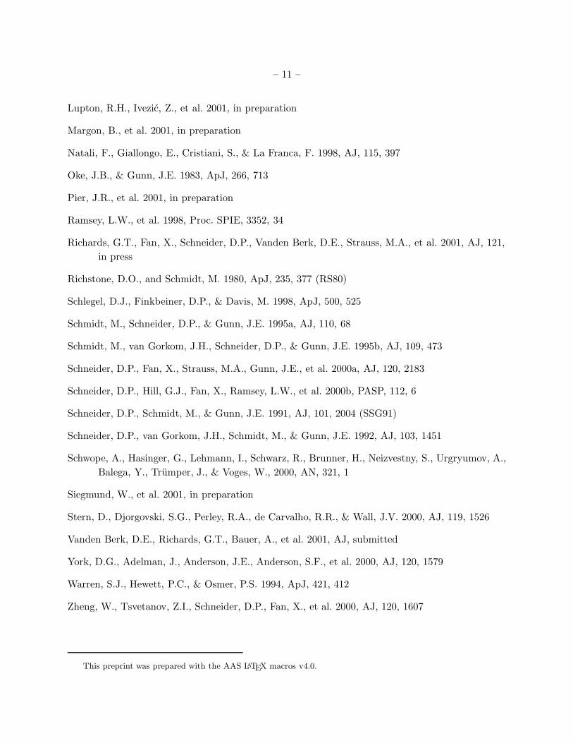
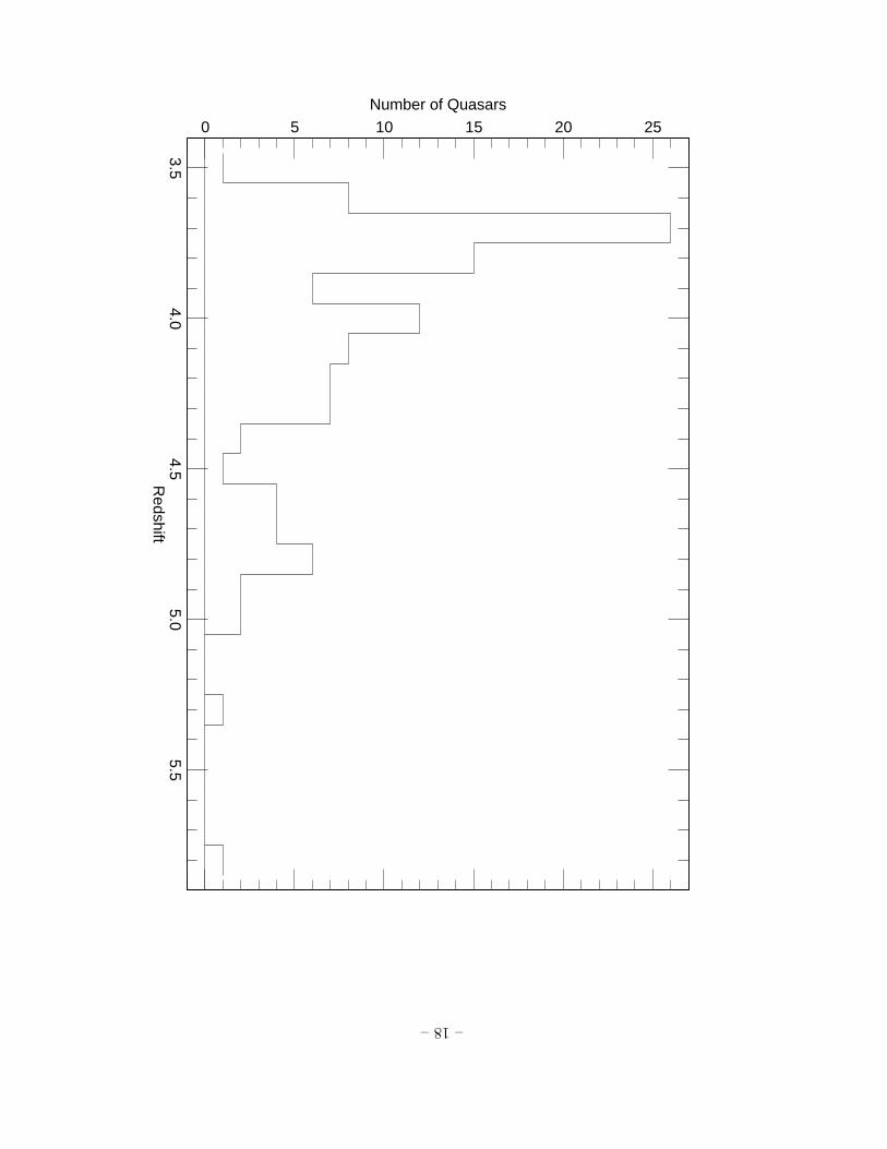
The redshift distribution of the SDSS quasars is displayed in Figure 4. The main features are

the sudden cutoff below z ≈ 3.6, which arises because of our reliance on the “g∗r∗i∗” color-color

plot (lower redshift quasars are found using the “u∗g∗r∗” diagram; see Richards et al. 2001), the

decline above z ≈ 3.7 due to the combination of the rapid fall of the quasar luminosity function

above z ≈ 3 (e.g., Schmidt et al. 1995a, Paper IV, and references therein) and the simple fact that

objects become fainter as the redshift increases, and the dip at z ≈ 4.5 discussed in the previous

paragraph.

The results here and in Paper III indicate that the SDSS will be able to efficiently identify

z ≈ 4 quasars at luminosities approximately one magnitude fainter than 3C 273. Paper III

and this paper mark the start of our attempt to assemble a complete sample of high-redshift

quasars to study the quasar luminosity function at considerably lower luminosities than that in

Paper IV, as well as investigate clustering of high-redshift quasars. To date, the SDSS quasars

have been spectroscopically confirmed “one-at-a time” with large telescopes (primarily the Apache

Point 3.5-m, HET, and Keck). In the past year the SDSS multifiber spectrographs have been

commissioned (see Castander et al. 2001), and spectra of more than 2000 quasars have been

analyzed at the time of this writing (Richards et al. 2001, Vanden Berk et al. 2001); this new

spectroscopic capability should lead to a rapid expansion of the number of known z > 3.5 quasars.

We would like to thank Ingo Lehmann for his expert help with determining the X-ray limits for

the objects, Pat Hall for useful comments on an early draft of the manuscript, and the entire HET

operations team for their efforts during the commissioning and early operations of the telescope.

– 9 –

This work was supported in part by National Science Foundation grants AST99-00703 (DPS

and GTR), AST00-71091 (MAS), and PHY00-70928 (XF). MAS and XF acknowledge additional

support from the Princeton University Research Board, and a Porter O. Jacobus Fellowship.

The Sloan Digital Sky Survey 17 (SDSS) is a joint project of the University of Chicago,

Fermilab, the Institute for Advanced Study, the Japan Participation Group, the Johns Hopkins

University, the Max-Planck-Institute for Astronomy, New Mexico State University, Princeton

University, the United States Naval Observatory, and the University of Washington. Apache Point

Observatory, site of the SDSS, is operated by the Astrophysical Research Consortium. Funding for

the project has been provided by the Alfred P. Sloan Foundation, the SDSS member institutions,

the National Aeronautics and Space Administration, the National Science Foundation, the

U.S. Department of Energy, Monbusho, and the Max Planck Society.

The Hobby-Eberly Telescope (HET) is a joint project of the University of Texas at Austin, the

Pennsylvania State University, Stanford University, Ludwig-Maximillians-Universitat Munchen,

and Georg-August-Universitat Gottingen. The HET is named in honor of its principal benefactors,

William P. Hobby and Robert E. Eberly. The Marcario Low Resolution Spectrograph is named

for Mike Marcario of High Lonesome Optics who fabricated several optics for the instrument but

died before its completion, and is a joint project of the Hobby-Eberly Telescope partnership and

the Instituto de Astronomia de la Universidad Nacional Autonoma de Mexico.

17The SDSS Web site is http://www.sdss.org/.

– 10 –

REFERENCES

Becker, R.H., White, R.L., & Helfand, D.J. 1995, ApJ, 450, 559

Brandt, W.N., Guainazzi, M., Kaspi, S., Fan, X., Schneider, D.P., Strauss, M.A., Clavel, J., &

Gunn, J.E. 2001, AJ, 121, in press

Carballo, R., Gonzalez-Serrano, J.I., Benn, C.R., Sanchez, S.F., & Vigotti, M. 1999, MNRAS, 306,

137

Castander, F.J., Nichol, R.C., et al. 2001, AJ, submitted

Cobos Duenas, F.J., Tejada, C., Hill, G.J., and Perez, G.F. 1998, Proc. SPIE, 3355, 424

Fan, X. 1999, AJ, 117, 2528

Fan, X., Strauss, M.A., Richards, G.T., Newman, J.A., et al. 2001a, AJ, 121, in press (Paper III)

Fan, X., Strauss, M.A., Schneider, D.P., Gunn, J.E., Lupton, R.H., Anderson, S.F., et al. 2000a,

AJ, 119, 1 (Paper II)

Fan, X., Strauss, M.A., Schneider, D.P., Gunn, J.E., Lupton, R.H., Yanny, B., et al. 1999, AJ,

118, 1 (Paper I)

Fan, X., Strauss, M.A., Schneider, D.P., Gunn, J.E., Lupton, R.H., Becker, R.H., et al. 2001b, AJ,

121, in press (Paper IV)

Fan, X., White, R.L., Davis, M., Becker, R.H., et al. 2000b, AJ, 120, 1167

Francis, P.J., Hewett, P.C., Foltz, C.B., Chaffee, F.H., Weymann, R.J., & Morris, S.L. 1991, ApJ,

373, 465

Fukugita, M., Ichikawa, T., Gunn, J.E., Doi, M., Shimasaku, K., & Schneider, D.P. 1996, AJ, 111,

1748

Gunn, J.E., Carr, M.A., Rockosi, C.M., Sekiguchi, M., et al. 1998, AJ, 116, 3040

Hill, G.J. 2000, Proc. SPIE, 4008, 50

Hill, G.J., Nicklas, H.E., MacQueen, P.J., Mitsch, W., Wellem, W., Altmann, W., Wesley, G.L., &

Ray, F.B. 1998a, Proc. SPIE, 3355, 433

Hill, G.J., Nicklas, H.E., MacQueen, P.J., Tejada, C., Cobos Duenas, F.J., & Mitsch, W. 1998b,

Proc. SPIE, 3355, 375

Kaspi, S., Brandt, W.N., & Schneider, D.P. 2000, AJ, 119, 2031

Lupton, R.H., Gunn, J.E., & Szalay, A. 1999, AJ, 118, 1406

– 11 –

Lupton, R.H., Ivezic, Z., et al. 2001, in preparation

Margon, B., et al. 2001, in preparation

Natali, F., Giallongo, E., Cristiani, S., & La Franca, F. 1998, AJ, 115, 397

Oke, J.B., & Gunn, J.E. 1983, ApJ, 266, 713

Pier, J.R., et al. 2001, in preparation

Ramsey, L.W., et al. 1998, Proc. SPIE, 3352, 34

Richards, G.T., Fan, X., Schneider, D.P., Vanden Berk, D.E., Strauss, M.A., et al. 2001, AJ, 121,

in press

Richstone, D.O., and Schmidt, M. 1980, ApJ, 235, 377 (RS80)

Schlegel, D.J., Finkbeiner, D.P., & Davis, M. 1998, ApJ, 500, 525

Schmidt, M., Schneider, D.P., & Gunn, J.E. 1995a, AJ, 110, 68

Schmidt, M., van Gorkom, J.H., Schneider, D.P., & Gunn, J.E. 1995b, AJ, 109, 473

Schneider, D.P., Fan, X., Strauss, M.A., Gunn, J.E., et al. 2000a, AJ, 120, 2183

Schneider, D.P., Hill, G.J., Fan, X., Ramsey, L.W., et al. 2000b, PASP, 112, 6

Schneider, D.P., Schmidt, M., & Gunn, J.E. 1991, AJ, 101, 2004 (SSG91)

Schneider, D.P., van Gorkom, J.H., Schmidt, M., & Gunn, J.E. 1992, AJ, 103, 1451

Schwope, A., Hasinger, G., Lehmann, I., Schwarz, R., Brunner, H., Neizvestny, S., Urgryumov, A.,

Balega, Y., Trumper, J., & Voges, W., 2000, AN, 321, 1

Siegmund, W., et al. 2001, in preparation

Stern, D., Djorgovski, S.G., Perley, R.A., de Carvalho, R.R., & Wall, J.V. 2000, AJ, 119, 1526

Vanden Berk, D.E., Richards, G.T., Bauer, A., et al. 2001, AJ, submitted

York, D.G., Adelman, J., Anderson, J.E., Anderson, S.F., et al. 2000, AJ, 120, 1579

Warren, S.J., Hewett, P.C., & Osmer, P.S. 1994, ApJ, 421, 412

Zheng, W., Tsvetanov, Z.I., Schneider, D.P., Fan, X., et al. 2000, AJ, 120, 1607

This preprint was prepared with the AAS LATEX macros v4.0.

– 12 –

Figure Captions

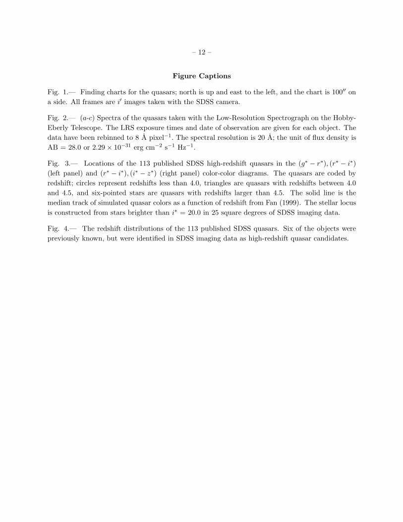
Fig. 1.— Finding charts for the quasars; north is up and east to the left, and the chart is 100′′ on

a side. All frames are i′ images taken with the SDSS camera.

Fig. 2.— (a-c) Spectra of the quasars taken with the Low-Resolution Spectrograph on the Hobby-

Eberly Telescope. The LRS exposure times and date of observation are given for each object. The

data have been rebinned to 8 A pixel−1. The spectral resolution is 20 A; the unit of flux density is

AB = 28.0 or 2.29 × 10−31 erg cm−2 s−1 Hz−1.

Fig. 3.— Locations of the 113 published SDSS high-redshift quasars in the (g∗ − r∗), (r∗ − i∗)

(left panel) and (r∗ − i∗), (i∗ − z∗) (right panel) color-color diagrams. The quasars are coded by

redshift; circles represent redshifts less than 4.0, triangles are quasars with redshifts between 4.0

and 4.5, and six-pointed stars are quasars with redshifts larger than 4.5. The solid line is the

median track of simulated quasar colors as a function of redshift from Fan (1999). The stellar locus

is constructed from stars brighter than i∗ = 20.0 in 25 square degrees of SDSS imaging data.

Fig. 4.— The redshift distributions of the 113 published SDSS quasars. Six of the objects were

previously known, but were identified in SDSS imaging data as high-redshift quasar candidates.

– 13 –

013932.68-010115.2 020731.68+010348.9 022239.42-005806.3 023446.58-001415.9 023908.98-002121.5

031036.85+005521.7 033910.53-003009.2 083929.33+003759.0084455.08+001848.5093556.92+002255.7

093931.91+003955.0094053.77+010514.4101832.46+001436.4 102846.10-010203.2 103848.12+004753.5

104837.40-002813.7 110813.86-005944.5

113559.94+002422.8

120210.09-005425.5 154014.57+001854.7

155923.86-000551.7 161544.14+010401.9225452.88+004822.7225624.35+004720.2230323.77+001615.2

230639.65+010855.2232201.37+000035.5 North

East i’ filter

60"

–14

–

Wavelength (A)

f nu 1

DN

= A

B 2

8

6000 7000 8000

050

010

0015

00

SDSSp J013932.68-010115.2 1800 s 121399

z = 3.69

Wavelength (A)

f nu 1

DN

= A

B 2

8

6000 7000 8000

010

0020

0030

0040

00

SDSSp J020731.68+010348.9 720 s 100799

z = 3.87

Wavelength (A)

f nu 1

DN

= A

B 2

8

6000 7000 8000

010

0020

0030

0040

00

SDSSp J022239.42-005806.3 720 s 101099

z = 3.63

Wavelength (A)

f nu 1

DN

= A

B 2

8

6000 7000 8000

020

0040

0060

0080

00

SDSSp J023446.58-001415.9 758 s 121099

z = 3.60

Wavelength (A)

f nu 1

DN

= A

B 2

8

6000 7000 8000

010

0020

0030

0040

00

SDSSp J023908.98-002121.5 600 s 101699

z = 3.73

Wavelength (A)

f nu 1

DN

= A

B 2

8

6000 7000 8000

010

0020

0030

0040

0050

00

SDSSp J031036.85+005521.7 1200 s 102099

z = 3.79

Wavelength (A)

f nu 1

DN

= A

B 2

8

6000 7000 8000

010

0020

0030

00

SDSSp J033910.53-003009.2 660 s 101499

z = 3.74

Wavelength (A)

f nu 1

DN

= A

B 2

8

6000 7000 8000

1000

2000

3000

4000

5000

6000

SDSSp J083929.33+003759.0 800 s 030800

z = 3.73

Wavelength (A)

f nu 1

DN

= A

B 2

8

6000 7000 8000

020

0040

0060

0080

00

SDSSp J084455.08+001848.5 600 s 031200

z = 3.69

–15

–

Wavelength (A)

f nu 1

DN

= A

B 2

8

6000 7000 8000

2000

4000

6000

8000

1000

0

SDSSp J093556.92+002255.7 900 s 030800

z = 3.73

Wavelength (A)

f nu 1

DN

= A

B 2

8

6000 7000 8000

050

010

0015

00

SDSSp J093931.91+003955.0 1062 s 032800

z = 4.49

Wavelength (A)

f nu 1

DN

= A

B 2

8

6000 7000 8000

010

0020

00

SDSSp J094053.77+010514.4 762 s 032900

z = 3.89

Wavelength (A)

f nu 1

DN

= A

B 2

8

6000 7000 8000

010

0020

0030

0040

00

SDSSp J101832.46+001436.4 1108 s 033000

z = 3.83

Wavelength (A)

f nu 1

DN

= A

B 2

8

6000 7000 8000

010

0020

0030

0040

0050

00

SDSSp J102846.10-010203.2 900 s 031500

z = 3.73

Wavelength (A)

f nu 1

DN

= A

B 2

8

6000 7000 8000

010

0020

0030

0040

00

SDSSp J103848.12+004753.5 600 s 031300

z = 3.74

Wavelength (A)

f nu 1

DN

= A

B 2

8

6000 7000 8000

020

0040

0060

0080

00

SDSSp J104837.40-002813.7 600 s 031000

z = 3.99

Wavelength (A)

f nu 1

DN

= A

B 2

8

6000 7000 8000

020

0040

0060

0080

00

SDSSp J110813.86-005944.5 600 s 031500

z = 4.01

Wavelength (A)

f nu 1

DN

= A

B 2

8

6000 7000 8000

010

0020

0030

0040

0050

0060

00

SDSSp J113559.94+002422.8 566 s 031500

z = 4.04

–16

–

Wavelength (A)

f nu 1

DN

= A

B 2

8

6000 7000 8000

050

0010

000

1500

020

000

2500

0

SDSSp J120210.09-005425.5 1200 s 030800

z = 3.59

Wavelength (A)

f nu 1

DN

= A

B 2

8

6000 7000 8000

010

0020

0030

00

SDSSp J154014.57+001854.7 762 s 031500

z = 3.83

Wavelength (A)

f nu 1

DN

= A

B 2

8

6000 7000 8000

010

0020

0030

0040

00

SDSSp J155923.86-000551.7 960 s 050800

z = 3.61

Wavelength (A)

f nu 1

DN

= A

B 2

8

6000 7000 8000

010

0020

0030

0040

0050

00

SDSSp J161544.14+010401.9 600 s 060200

z = 4.01

Wavelength (A)

f nu 1

DN

= A

B 2

8

6000 7000 8000

020

0040

0060

0080

00

SDSSp J225452.88+004822.7 900 s 111299

z = 3.70

Wavelength (A)

f nu 1

DN

= A

B 2

8

6000 7000 8000

010

0020

0030

0040

00

SDSSp J225624.35+004720.2 780 s 111099

z = 4.08

Wavelength (A)

f nu 1

DN

= A

B 2

8

6000 7000 8000

025

0050

0075

0010

000

SDSSp J230323.77+001615.2 753 s 101299

z = 3.70

Wavelength (A)

f nu 1

DN

= A

B 2

8

6000 7000 8000

020

0040

0060

0080

00

SDSSp J230639.65+010855.2 600 s 111099

z = 3.64

Wavelength (A)

f nu 1

DN

= A

B 2

8

6000 7000 8000

010

0020

0030

00

SDSSp J232201.37+000035.5 600 s 101099

z = 3.84

– 17 –

–18–

Redshift

Number of Quasars

3.54.0

4.55.0

5.5

0 5 10 15 20 25

– 19 –

TABLE 1. Positions and Photometry of SDSS High-Redshift Quasars

Quasar (SDSSp J) Redshift u∗ g∗ r∗ i∗ z∗ Run

013932.68−010115.2 3.69 ± 0.01 25.14 ± 0.85 22.09 ± 0.10 21.01 ± 0.05 20.97 ± 0.08 20.67 ± 0.23 94

020731.68+010348.9 3.87 ± 0.02 23.93 ± 0.41 21.20 ± 0.04 20.04 ± 0.02 19.89 ± 0.03 19.75 ± 0.11 94

022239.42−005806.3 3.63 ± 0.01 24.23 ± 0.59 21.31 ± 0.05 20.23 ± 0.03 20.08 ± 0.04 19.95 ± 0.14 94

023446.58−001415.9 3.60 ± 0.02 23.91 ± 0.64 21.40 ± 0.06 20.24 ± 0.03 20.10 ± 0.03 20.35 ± 0.15 125

023908.98−002121.5* 3.73 ± 0.03 24.85 ± 0.78 20.99 ± 0.04 19.62 ± 0.02 19.54 ± 0.02 19.33 ± 0.07 125

031036.85+005521.7 3.79 ± 0.01 23.24 ± 0.54 20.99 ± 0.04 19.50 ± 0.02 19.31 ± 0.02 19.16 ± 0.06 125

033910.53−003009.2 3.74 ± 0.01 23.30 ± 0.57 21.30 ± 0.04 20.09 ± 0.02 19.96 ± 0.03 19.72 ± 0.10 125

083929.33+003759.0* 3.73 ± 0.03 23.55 ± 0.49 20.52 ± 0.03 19.28 ± 0.02 19.19 ± 0.02 18.95 ± 0.04 756

084455.08+001848.5 3.69 ± 0.01 23.06 ± 0.36 21.34 ± 0.04 19.94 ± 0.02 19.85 ± 0.03 19.85 ± 0.09 756

093556.92+002255.7 3.73 ± 0.01 25.03 ± 0.44 19.83 ± 0.03 18.69 ± 0.02 18.55 ± 0.02 18.40 ± 0.04 756

093931.91+003955.0 4.49 ± 0.01 22.89 ± 0.37 24.32 ± 0.44 21.61 ± 0.07 20.62 ± 0.05 20.47 ± 0.14 756

094053.77+010514.4 3.89 ± 0.01 23.93 ± 0.43 21.70 ± 0.06 20.45 ± 0.04 20.26 ± 0.04 20.17 ± 0.13 756

101832.46+001436.4 3.83 ± 0.01 24.12 ± 0.51 21.63 ± 0.05 20.23 ± 0.03 20.09 ± 0.03 19.87 ± 0.09 756

102846.10−010203.2 3.73 ± 0.01 23.91 ± 0.50 21.02 ± 0.04 19.69 ± 0.02 19.57 ± 0.02 19.54 ± 0.07 756

103848.12+004753.5 3.74 ± 0.01 22.46 ± 0.19 20.77 ± 0.03 19.64 ± 0.02 19.56 ± 0.02 19.32 ± 0.05 756

104837.40−002813.7 3.99 ± 0.02 24.88 ± 0.57 20.87 ± 0.04 19.27 ± 0.02 19.04 ± 0.06 18.97 ± 0.13 756

110813.86−005944.5 4.01 ± 0.01 23.72 ± 0.44 21.01 ± 0.03 19.56 ± 0.01 19.29 ± 0.02 19.14 ± 0.05 756

113559.94+002422.8 4.04 ± 0.01 23.62 ± 0.35 21.37 ± 0.05 20.03 ± 0.03 19.88 ± 0.03 19.73 ± 0.08 756

120210.09−005425.5 3.59 ± 0.01 23.54 ± 0.58 20.10 ± 0.02 19.05 ± 0.01 18.94 ± 0.01 18.93 ± 0.04 756

154014.57+001854.7 3.83 ± 0.02 24.64 ± 0.52 21.75 ± 0.05 20.42 ± 0.04 20.26 ± 0.04 20.34 ± 0.17 756

155923.86−000551.7 3.61 ± 0.01 23.59 ± 0.46 21.79 ± 0.05 20.65 ± 0.03 20.47 ± 0.04 20.63 ± 0.18 745

161544.14+010401.9 4.01 ± 0.01 24.33 ± 0.62 21.74 ± 0.05 20.34 ± 0.02 20.22 ± 0.04 20.20 ± 0.13 745

225452.88+004822.7 3.70 ± 0.01 23.01 ± 0.55 21.52 ± 0.07 20.26 ± 0.03 20.13 ± 0.05 19.94 ± 0.16 94

225624.35+004720.2 4.08 ± 0.01 23.75 ± 0.80 21.96 ± 0.10 20.28 ± 0.04 20.17 ± 0.07 19.94 ± 0.16 94

230323.77+001615.2 3.70 ± 0.01 25.31 ± 0.39 21.22 ± 0.05 20.11 ± 0.03 20.07 ± 0.04 20.03 ± 0.20 94

230639.65+010855.2 3.64 ± 0.01 23.91 ± 0.51 20.59 ± 0.03 19.25 ± 0.01 19.00 ± 0.02 18.84 ± 0.06 94

232201.37+000035.5 3.84 ± 0.01 24.55 ± 0.60 21.34 ± 0.05 20.19 ± 0.03 20.07 ± 0.04 20.01 ± 0.15 94

Notes: Positions are in J2000.0 coordinates. An asterisk following an object name indicates a BAL quasar.

Photometry is reported in terms of asinh magnitudes; see Lupton, Gunn, & Szalay (1999) for details. In this system,

zero flux corresponds to 23.24, 24.91, 24.53, 23.89, and 22.47 in u∗, g∗, r∗, i∗, and z∗, respectively.

– 20 –

TABLE 2. Properties of SDSS High-Redshift Quasars

Quasar (SDSSp J) Redshift E(B − V ) AB1450 α ∆Lα M1450

013932.68−010115.2 3.69 0.034 21.08 −0.93 5.1 −24.65

020731.68+010348.9 3.87 0.026 20.00 −0.96 −2.3 −25.80

022239.42−005806.3 3.63 0.036 20.27 −0.91 1.2 −25.43

023446.58−001415.9 3.60 0.022 20.40 −0.89 1.0 −25.29

023908.98−002121.5* 3.73 0.028 19.53 −0.92 8.4 −26.21

031036.85+005521.7 3.79 0.115 19.18 −0.76 8.1 −26.59

033910.53−003009.2 3.74 0.104 19.90 −1.14 2.6 −25.85

083929.33+003759.0* 3.73 0.042 19.14 −0.84 22.1 −26.60

084455.08+001848.5 3.69 0.035 20.05 −1.11 −0.6 −25.68

093556.92+002255.7 3.73 0.050 18.61 −1.03 15.2 −27.13

093931.91+003955.0 4.49 0.065 20.52 −0.42 13.4 −25.51

094053.77+010514.4 3.89 0.097 20.29 −0.28 −1.8 −25.52

101832.46+001436.4 3.83 0.043 20.19 −1.09 0.5 −25.59

102846.10−010203.2 3.72 0.052 19.72 −1.17 1.3 −26.02

103848.12+004753.5 3.74 0.060 19.54 −0.65 17.5 −26.21

104837.40−002813.7 3.99 0.040 19.08 −1.19 10.3 −26.77

110813.86−005944.5 4.01 0.047 19.35 −1.01 4.0 −26.51

113559.94+002422.8 4.04 0.019 19.96 −0.95 4.9 −25.91

120210.09−005425.5 3.59 0.025 19.25 −0.91 2.0 −26.43

154014.57+001854.7 3.83 0.093 20.20 −0.57 13.7 −25.59

155923.86−000551.7 3.61 0.126 20.51 −1.58 2.8 −25.18

161544.14+010401.9 4.01 0.091 20.18 −0.88 1.0 −25.68

225452.88+004822.7 3.70 0.087 20.22 −1.11 1.5 −25.51

225624.35+004720.2 4.08 0.059 20.14 −0.25 4.4 −25.75

230323.77+001615.2 3.70 0.049 20.18 −0.93 1.4 −25.55

230639.65+010855.2 3.64 0.053 19.15 −1.58 1.3 −26.56

232201.37+000035.5 3.84 0.043 20.13 −1.14 4.5 −25.66

Notes: An asterisk following an object name indicates a BAL quasar. Galactic reddening values

from Schlegel, Finkbeiner, & Davis (1998), and a standard reddening law R = 3.1 were used to

calculate AB1450. The absolute magnitude M1450 was calculated assuming H0 = 50 km s−1 Mpc−1,

Ω0 = 1, and Λ = 0. Absolute B magnitudes can be calculated from MB = M1450 + 1.21α + 0.12,

where α is the spectral power law index (fν ∝ να) between the rest frame ultraviolet and blue;

MB = M1450 − 0.49 for α = −0.5.