High-pressure vapor–liquid equilibria in the nitrogen–n-pentane system

A

5ewamt©

K

1

gemstftltfcHoiNo

0d

J. of Supercritical Fluids 42 (2007) 36–47

High-pressure vapor–liquid equilibria in the nitrogen–n-nonane system

Guadalupe Silva-Oliver a,b, Gaudencio Eliosa-Jimenez a,Fernando Garcıa-Sanchez a,∗, Juan Ramon Avendano-Gomez b

a Laboratorio de Termodinamica, Programa de Ingenierıa Molecular, Instituto Mexicano del Petroleo,Eje Central Lazaro Cardenas 152, 07730 Mexico, D.F., Mexico

b Departamento de Ingenierıa Quımica Petrolera y Laboratorio de Investigacion en Ingenierıa Quımica Ambiental, ESIQIE,Instituto Politecnico Nacional, Unidad Profesional Adolfo Lopez Mateos, Zacatenco, 07738 Mexico, D.F., Mexico

Received 28 July 2006; received in revised form 24 January 2007; accepted 25 January 2007

bstract

New experimental vapor–liquid equilibrium data of the N2–n-nonane system were measured over a wide temperature range from 344.3 to43.4 K and pressures up to 50 MPa. A static-analytical apparatus with visual sapphire windows and pneumatic capillary samplers was used in thexperimental measurements. Equilibrium phase compositions and vapor–liquid equilibrium ratios are reported. The new results were comparedith those reported by other authors. The comparison showed that the pressure-liquid phase composition data reported in this work are in good

greement with those determined by others. The experimental data were modeled with the PR and PC-SAFT equations of state by using one-fluidixing rules and a single temperature-independent interaction parameter. Results of the modeling showed that the PC-SAFT equation was superior

o the PR equation in correlating the experimental data of the N2–n-nonane system.2007 Elsevier B.V. All rights reserved.

tabili

mittNptNqtNlci

eywords: Vapor–liquid equilibria; Enhanced oil recovery; Equation of state; S

. Introduction

An optimal recovery strategy in enhanced oil recovery byas N2 injection requires of extensive knowledge of the phasequilibria and physicochemical properties inherent to the ther-odynamic systems found at reservoir conditions. A literature

urvey of the phase behavior of N2-containing systems showedhat all binary N2–hydrocarbon fluid mixtures develop, exceptor methane, type III phase diagrams according to the classifica-ion scheme of van Konynenburg and Scott [1]; i.e., one criticaline going from the component with the lower critical tempera-ure to an upper critical endpoint and a second critical line goingrom the component with the higher critical temperature to aritical point in a dense mixture at extremely high pressures.ence, a comprehensive understanding of the phase behaviorf the N2 and the crude oil is essential for applications of N2
n enhanced oil recovery; e.g., the equilibrium phase diagram of
2–crude oil systems can be used to establish whether a miscibler immiscible condition will occur.

∗ Corresponding author. Tel.: +52 55 9175 6574; fax: +52 55 9175 6380.E-mail address: [email protected] (F. Garcıa-Sanchez).

atawtab

896-8446/$ – see front matter © 2007 Elsevier B.V. All rights reserved.oi:10.1016/j.supflu.2007.01.006

ty analysis; Phase envelope; Critical point

In practice, the phase behavior of these multicomponentixtures is predicted by using equations of state. However,

t is difficult to use these equations to predict correctlyhe complex phase behavior of N2–crude oil systems dueo a lack of experimental phase equilibrium information of

2–hydrocarbon systems over wide ranges of temperature andressure. In fact, most of the information on this subject referso binary N2–hydrocarbon systems [2–52] and only a few

2–hydrocarbon data are reported for ternary [10,15,35,53–58],uaternary [35,59], and multicomponent [60] systems. Never-heless, as pointed out by Grausø et al. [9], many of the binary

2–hydrocarbon vapor–liquid equilibrium data reported in theiterature are generally not internally consistent and mutuallyonflicting; i.e., there is a great deal of scatter among the exper-mental points.

On the basis of the above, it is necessary to carry outdditional experimental phase equilibrium studies at elevatedemperatures and pressures of N2-containing binary systemslong with experimental fitting using thermodynamic models. It
ill ensure the right qualitative and quantitative description of
he phase behavior of N2–hydrocarbon mixtures and will providebetter understanding of phase behavior patterns that hydrocar-on mixtures develop during an enhanced oil recovery process

mailto:[email protected]

dx.doi.org/10.1016/j.supflu.2007.01.006

G. Silva-Oliver et al. / J. of Supercritical Fluids 42 (2007) 36–47 37

Nomenclature

a attractive term in PR EoSa reduced Helmholtz energy, a = A/NkBT

A Helmholtz energy (J)b co-volume in PR EoSd temperature dependent segment diameter (A)ghs

αβ site-site radial distribution function of hard-sphere fluid

I1, I2 abbreviations, defined by Eqs. (B.13) and (B.14)kB Boltzmann constant (J K−1)kij binary interaction parameterKi equilibrium ratio of component i, Ki = yi/xi

m number of segments per chainm mean segment number in the system, defined in

Eq. (B.3)P pressure (MPa)R gas constantRi chromatographic response coefficient to compo-

nent iRij ratio of chromatographic response coefficients,

Rij = Ri/Rj

S1 objective function, defined in Eq. (4)S2 objective function, defined in Eq. (5)Si chromatographic peak area for component iSji ratio of chromatographic peak areas, Sji = Sj/Si

T temperature (K)v molar volumexi liquid mole fraction of component iyi vapor mole fraction of component iZ compressibility factor, Z = Pv/(RT )

Greek lettersα alpha function in PR EoSη packing fraction, η = ζ3ϕi fugacity coefficient of component iρ total number density of molecules (A−3)σ segment diameter (A)σP standard percent relative deviation in pressure,

defined in Eq. (6)σx standard percent deviation in liquid mole fraction,

defined in Eq. (7)σy standard percent deviation in vapor mole fraction,

defined in Eq. (8)ω acentric factor in PR EoSζn abbreviation (n = 0, . . ., 3), defined by Eq. (B.6)

(An−3)

Superscriptscalc calculated propertydisp contribution due to dispersive attractionexp experimental propertyhc residual contribution of hard-chain systemhs residual contribution of hard-sphere systemres residual property

Subscripts

baapM

srihtmsicr

mToid

2

2

Gtp9c

2

watct

ltrsc

u

c critical propertyi, j components i, j

y N2 injection. Toward this end, we have undertaken a system-tic study of the phase behavior of N2–hydrocarbon mixturest high pressures. This study is part of a research project wherehase behavior is studied for enhanced oil recovery in selectedexican fields by N2 injection.In this work, we report new vapor–liquid equilibrium mea-

urements for the system N2–n-nonane over a temperatureange from 344.3 to 543.4 K and pressures up to 50 MPa. Fivesotherms are reported in this study, which were determined in aigh-pressure phase equilibrium facility of the static-analyticalype. The apparatus uses a sampling-analyzing process for deter-

ining the composition of the different coexisting phases. Thisampling-analyzing system consists of a series of RolsiTM cap-llary samplers [61] connected altogether on-line with a gashromatograph that makes the apparatus very practical and accu-ate for measurements at high temperatures and pressures.

The experimental data obtained in our measurements wereodeled using the PR [62] and PC-SAFT [63] equations of state.he mixing rules used for these equations were the classicalne-fluid mixing rules. For both models, a single temperature-ndependent interaction parameter was fitted to all experimentalata.

. Experimental

.1. Materials

Nitrogen and helium (carrier gas) were acquired from Agaas (Mexico) and Infra (Mexico), respectively, both with a cer-

ified purity greater than 99.999 mol%. Nonane normal wasurchased from Aldrich (USA) with a minimum purity of9 mol%. The chemicals were used without any further purifi-ation except for careful degassing of the n-nonane.

.2. Apparatus and procedure

The experimental apparatus (Armines, France) used in thisork is schematically shown in Fig. 1. It is based on the static-

nalytical method with fluid phase sampling, and can be usedo determine the multiphase equilibrium of binary and multi-omponent systems between 313 and 673 K, and pressures upo 60 MPa.

This apparatus consists mainly of the following: an equi-ibrium cell, three pneumatic capillary samplers, a pressureransducer, two platinum temperature sensors, a magnetic stir-ing device, a timer and compressed-air control device for each
ampler, an analytical system, and feeding and degassing cir-uits.
The equilibrium cell, made of titanium, has an internal vol-me of about 100 mL and holds two sapphire windows for visual

38 G. Silva-Oliver et al. / J. of Supercritical Fluids 42 (2007) 36–47

f the

omscato

tsvtdsmatp

6icvotte

(cs

(u

stetatrIBItht

sw

Fig. 1. Schematic diagram o

bservation of the coexisting phases. The cap of the cell (alsoade out of titanium) holds three fixed pneumatic capillary

amplers (for studies with up to three coexisting phases) withapillaries of different lengths: the extremity of one capillary ist the top of the cell (vapor withdrawing), another one at the bot-om of the cell (withdrawing of the dense liquid), and the thirdne in an intermediate position (light liquid phase withdrawing).

The pneumatic samplers, being heated independently fromhe vessel or tubing containing the fluid to be sampled, arepecially adapted to the study of fluid phase equilibria (i.e.,apor–liquid, liquid–liquid, vapor–liquid–liquid . . .) becausehey allow very small samples to be withdrawn without anyisturbance of equilibrium. The fast transfer of the totality ofamples, from the equilibrium cell up to the column of chro-atograph, ensures reliability. Withdrawn quantities are roughly

djusted by means of a differential screw acting on the stroke ofhe bellows, and a fine adjustment is obtained in the backwardart of the sampler through a timer.

The pressure transducer (Sensonetics for temperatures up to73 K) is connected to the cell by heating capillary tubing. Its thermoregulated to avoid condensation and ensuring the bestonditions. On one side of the cell there are two high-pressurealves (Autoclave Engineers) for liquid and gas feeding. On the
ther side, two wells were drilled inside the cylindrical wall ofhe cell body: one at the top and the other at the bottom to receivehe temperature sensors. A magnetic rod is used to achieve anfficient stirring inside the equilibrium cell. The magnetic rod
bito

static-analytical apparatus.

Hastelloy covered) is rotated using a magnet, external to theell, and driven through a variable speed motor mounted on atirring device.

All the electronics connected to the measurement devicespressure transducer, temperature probes, monitoring of the liq-id and vapor samplers) are gathered into a monitor box.

The cell is placed in a high temperature regulating air thermo-tat (Spame, France), which controls and maintains the desiredemperature within ±0.2 K. Temperature measurements in thequilibrium cell were monitored by using two Pt100 resistancehermometers located at the top and bottom of the cell, whichllows checking of the thermal gradients. The two Pt100 resis-ances thermometers are periodically calibrated against a 25

eference platinum resistance thermometer (Tinsley Precisionnstruments), which was previously calibrated by the Nationalureau of Metrology (CENAM, Mexico) based on the 1990

nternational Temperature Scale (ITS 90). The resulting uncer-ainty of the two Pt100 probes was not higher than ±0.02 K;owever, drift in the temperature of the oven makes the uncer-ainty of the temperature measurements to be ±0.2 K.

Pressure measurements were carried out by means of a pres-ure transducer (Sensonetics, model SEN-401-7.5M-12-6-C1),hich is periodically calibrated against a dead-weight pressure
alance (DH-Budenberg, model 5203). This pressure transducers maintained at constant temperature (temperature higher thanhe highest temperature of study) by means of a specially madeven, which is controlled using a proportional regulator (West,

percr

mt

mcscSTINrifDb

actts

dtTtTef4iptpfp5rParaccvclRr

stwdtw

3

Lci

bTtinlm

z

w

�

w

�

woafi

teert

drs

TS

R

LT

G. Silva-Oliver et al. / J. of Su

odel 6100). Pressure measurement uncertainties are estimatedo be within ±0.02 MPa for pressures up to 50 MPa.

The analytical work was carried out by using a gas chro-atograph (Varian, model 3800) equipped with a thermal

onductivity detector (TCD), which is connected to a data acqui-ition system (Star GC Workstation, Version 5.3). The analyticalolumn used is a Restek 3% OV-101 column (mesh 100/120ilcoport-W, silcosteel tube, length: 3 m, diameter: 3.175 mm).he TCD was used to detect the n-nonane and N2 compounds.

t was calibrated by injecting known amounts of n-nonane and2 through liquid-tight (5 �L) and gas-tight (1000 �L) syringes,

espectively. Calibration data were fitted to a straight line, lead-ng to an estimated mole fraction uncertainty less than 1%or liquid and vapor phases on the whole concentration range.etails of the calibration procedure and the calibration data cane found elsewhere [64].

Once the pressure transducer, platinum temperature probes,nd chromatographic thermal conductivity detector have beenalibrated, the system was preflushed with isopropyl alcohol andhen dried under vacuum at 423 K. After drying under vacuum,he system was purged with N2 to ensure that the last traces ofolvents were removed.

During an experimental run, the liquid component, previouslyegassed in one of the degassing cells (see Fig. 1) according tohe method of Battino et al. [65], is first introduced into the cell.he equilibrium cell and its loading lines are evacuated down

o 0.1 Pa before filling it with the degassed liquid component.he liquid component is then introduced by gravity into thequilibrium cell via valve 4. In this case, the gravity push wasast enough to prevent the entering fluid from flashing. Valveis then closed and the temperature in the air bath thermostat

s adjusted at the top and bottom of the cell to the same tem-erature by means of the heating resistances. Once the desiredemperature is reached and stabilized, the gaseous component,reviously stored in a stainless steel high-pressure cell, is care-ully introduced into the equilibrium cell via valve 5 until aressure slightly lower to that pressure of measurement. Valveis then closed and the magnetic stirring device is activated to

each equilibrium, which is indicated by pressure stabilization.ressure is adjusted by injecting again the gaseous componentnd activating the stirring device until the desired pressure iseached. After equilibrium in the cell is achieved, measurementsre performed using the capillary-sampling injectors, which areonnected to the equilibrium cell by 0.1 mm internal diameterapillary tubes of different length. The samples are injected andaporized directly into the carrier gas (helium) stream of the gas
hromatograph. For each equilibrium condition, at least 25 equi-ibrium samples are withdrawn using the pneumatic samplersolsiTM and analyzed in order to check for measurement and
epeatability. As the volume of the withdrawn samples is very

obcl

able 1ummary of vapor–liquid equilibria for the N2–n-nonane system

eference Temperature range (K) Pressu

lave and Chung [35] 322.0–344.3 3.72–3his work 344.3–543.4 1.97–4

itical Fluids 42 (2007) 36–47 39

mall compared to the volume of the vapor or liquid present inhe equilibrium cell, it is possible to withdraw many samplesithout disturbing the phase equilibrium. In order to avoid con-ensation and adsorption of n-nonane, the samplers and all ofhe lines for the gas stream are superheated to ensure that thehole of the samples is transferred to the chromatograph.

. Experimental results

The N2–n-nonane system has been previously studied bylave and Chung [35] at different temperature and pressureonditions. Table 1 contains a summary of the earlier results,ncluding those presented in this paper.

The new measured equilibrium phase compositions for thisinary system, temperatures, and pressures, are tabulated inable 2. Uncertainties in the phase compositions, due mainly

o errors associated with sampling, are estimated to be ±0.003n the mole fraction, although this may be as large as ±0.005ear the critical region. Error calculations were performed as fol-ows: from Eq. (1) relating mole fractions zi to chromatographic

easurements

i = 1

1 +∑j �=iRijSji

, zi = xi or yi (1)

e have the errors given by

zi = z2i

∑j �=i

(Rij �Sji + Sji �Rij) (2)

ith

Rij = (�R2i + �R2

j )1/2

(3)

here �Sji is estimated from the dispersion of Si and Sj valuesbtained by analyses on a least five samples, and �Ri and �Rj

re the mean quadratic relative deviations resulting from a datatting on the results of the chromatograph detector calibration.

Table 2 also presents the vapor pressures of n-nonane at eachemperature level. These values were calculated with the Wagnerquation in the “3, 6” form using the parameters reported by Reidt al. [66]. The calculated K-values, defined as the equilibriumatio between the vapor and liquid for each component at a givenemperature and pressure, are also given in this table.

Fig. 2 shows the results obtained on a pressure-compositioniagram for the various experimental temperatures, including theesults of Llave and Chung [35]. An examination of this figurehows that our liquid-phase composition results at temperature
f 344.3 K are in very good agreement with those determinedy these investigators at the same temperature. In this figure, itan be observed that the solubility of N2 in the n-nonane-richiquid phase increases as pressure increases for all isotherms
re range (MPa) Number of points Remarks

4.74 12 P–x data9.75 70 P–x–y data

40 G. Silva-Oliver et al. / J. of Supercritical Fluids 42 (2007) 36–47

Table 2Experimental vapor–liquid equilibrium data for the system N2–n-nonane

T (K) P (MPa) xN2 yN2 KN2 KnC9

344.3 0.007a 0.0000 0.00002.34 0.0310 0.9852 31.7806 0.01533.50 0.0456 0.9904 21.7193 0.01015.36 0.0695 0.9932 14.2906 0.00737.15 0.0905 0.9940 10.9834 0.00669.82 0.1195 0.9944 8.3213 0.0064

13.72 0.1589 0.9944 6.2580 0.006717.24 0.1906 0.9942 5.2162 0.007220.59 0.2203 0.9936 4.5102 0.008224.03 0.2483 0.9929 3.9988 0.009427.48 0.2763 0.9921 3.5907 0.010931.02 0.3032 0.9915 3.2701 0.012234.46 0.3268 0.9904 3.0306 0.014337.74 0.3486 0.9892 2.8376 0.016641.65 0.3746 0.9879 2.6372 0.019345.72 0.3969 0.9860 2.4843 0.023249.58 0.4189 0.9835 2.3478 0.0284

423.5 0.10a 0.0000 0.00002.44 0.0374 0.9494 25.3850 0.05263.18 0.0484 0.9577 19.7872 0.04453.84 0.0587 0.9625 16.3969 0.03984.77 0.0732 0.9679 13.2227 0.03467.37 0.1120 0.9741 8.6973 0.02929.65 0.1437 0.9770 6.7989 0.0269

14.71 0.2096 0.9775 4.6636 0.028519.86 0.2716 0.9772 3.5979 0.031324.73 0.3248 0.9740 2.9988 0.038529.83 0.3823 0.9708 2.5394 0.047334.36 0.4295 0.9676 2.2529 0.056839.75 0.4814 0.9627 1.9998 0.071944.08 0.5188 0.9553 1.8414 0.092949.75 0.5741 0.9466 1.6488 0.1254

473.4 0.32a 0.0000 0.00002.49 0.0382 0.8366 21.9005 0.16993.79 0.0626 0.8867 14.1645 0.12095.29 0.0891 0.9114 10.2290 0.09737.56 0.1274 0.9271 7.2771 0.0835

10.34 0.1736 0.9366 5.3952 0.076715.06 0.2489 0.9408 3.7798 0.0788

473.4 19.49 0.3134 0.9393 2.9971 0.088425.25 0.3962 0.9320 2.3523 0.112629.76 0.4607 0.9230 2.0035 0.142835.00 0.5426 0.9067 1.6710 0.204037.55 0.5843 0.8963 1.5340 0.249539.95 0.6299 0.8753 1.3896 0.336941.51 0.6688 0.8484 1.2685 0.4577

508.1 0.61a 0.0000 0.00001.97 0.0293 0.6193 21.1365 0.39223.67 0.0649 0.7698 11.8613 0.24625.14 0.0949 0.8193 8.6333 0.19967.63 0.1443 0.8581 5.9466 0.1658

10.08 0.1925 0.8749 4.5449 0.154912.55 0.2398 0.8816 3.6764 0.155715.01 0.2879 0.8835 3.0688 0.163617.57 0.3360 0.8825 2.6265 0.177020.03 0.3807 0.8767 2.3029 0.199122.66 0.4338 0.8688 2.0028 0.231725.08 0.4803 0.8564 1.7831 0.276327.41 0.5348 0.8376 1.5662 0.349129.79 0.6203 0.7897 1.2731 0.5539

Table 2 (Continued )

T (K) P (MPa) xN2 yN2 KN2 KnC9

543.4 1.10a 0.0000 0.00002.08 0.0255 0.3639 14.2706 0.65272.61 0.0393 0.4580 11.6539 0.56423.28 0.0564 0.5434 9.6348 0.48394.19 0.0800 0.6126 7.6575 0.42115.35 0.1089 0.6685 6.1387 0.37206.69 0.1431 0.7050 4.9266 0.34438.14 0.1804 0.7309 4.0516 0.32839.60 0.2184 0.7458 3.4148 0.3252

11.05 0.2573 0.7540 2.9304 0.331212.52 0.2960 0.7601 2.5679 0.340814.08 0.3395 0.7583 2.2336 0.365915.55 0.3810 0.7461 1.9583 0.4102

irtpbc

(sapiow

FsL

17.10 0.4331 0.7290 1.6832 0.478018.32 0.4879 0.6976 1.4298 0.5905

a Calculated vapor pressure of pure n-nonane [66].

nvestigated. However, the solubility of N2 in the n-nonane-ich liquid phase decreases with decreasing temperature; i.e.,he N2–n-nonane system exhibits the reverse order solubilityhenomenon, which is opposite of what normally occurs for ainary mixture of a supercritical component and a subcriticalomponent.

Isotherms obtained above the critical temperature of N2Tc = 126.2 K) end up in the mixture critical point. Notwith-tanding, it was very difficult to distinguish between the vapornd liquid phases when the mixture was approaching the critical
oint since the meniscus became very diffuse. The mixture crit-cal point was approached by adding carefully small quantitiesf N2 in order to avoid upsetting the phase equilibrium. It isorth noting that the measurements at 508.1 K and 29.79 MPa
ig. 2. Experimental pressure-composition phase diagram for the N2–n-nonaneystem. Full circles: data reported in this work; open symbols: data taken fromlave and Chung [35].

G. Silva-Oliver et al. / J. of Supercritical Fluids 42 (2007) 36–47 41

Table 3Mixture critical data of the N2–n-nonane system

T (K) P (MPa) xN2 T (K) P (MPa) xN2

473.4 42.48 0.7659 543.4 19.12 0.58775

wpctthiswa1

tetctwbpcmmtpTfs

letdmtscjcmc[

iubv(i

Fs

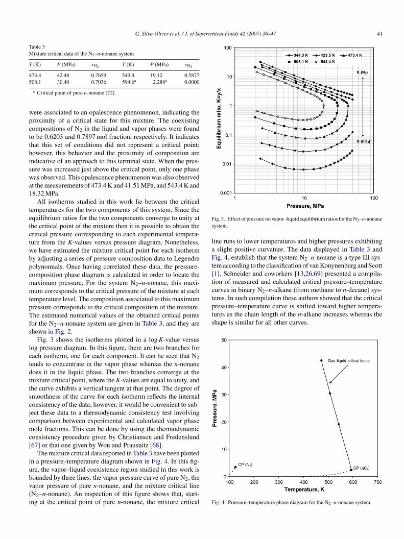
laFt[tctems. In such compilation these authors showed that the criticalpressure–temperature curve is shifted toward higher tempera-tures as the chain length of the n-alkane increases whereas theshape is similar for all other curves.

08.1 30.40 0.7036 594.6a 2.288a 0.0000

a Critical point of pure n-nonane [72].

ere associated to an opalescence phenomenon, indicating theroximity of a critical state for this mixture. The coexistingompositions of N2 in the liquid and vapor phases were foundo be 0.6203 and 0.7897 mol fraction, respectively. It indicateshat this set of conditions did not represent a critical point;owever, this behavior and the proximity of composition arendicative of an approach to this terminal state. When the pres-ure was increased just above the critical point, only one phaseas observed. This opalescence phenomenon was also observed

t the measurements of 473.4 K and 41.51 MPa, and 543.4 K and8.32 MPa.

All isotherms studied in this work lie between the criticalemperatures for the two components of this system. Since thequilibrium ratios for the two components converge to unity athe critical point of the mixture then it is possible to obtain theritical pressure corresponding to each experimental tempera-ure from the K-values versus pressure diagram. Nonetheless,e have estimated the mixture critical point for each isothermy adjusting a series of pressure-composition data to Legendreolynomials. Once having correlated these data, the pressure-omposition phase diagram is calculated in order to locate theaximum pressure. For the system N2–n-nonane, this maxi-um corresponds to the critical pressure of the mixture at each

emperature level. The composition associated to this maximumressure corresponds to the critical composition of the mixture.he estimated numerical values of the obtained critical points

or the N2–n-nonane system are given in Table 3, and they arehown in Fig. 2.

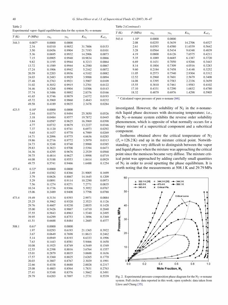
Fig. 3 shows the isotherms plotted in a log K-value versusog pressure diagram. In this figure, there are two branches forach isotherm, one for each component. It can be seen that N2ends to concentrate in the vapor phase whereas the n-nonaneoes it in the liquid phase. The two branches converge at theixture critical point, where the K-values are equal to unity, and

he curve exhibits a vertical tangent at that point. The degree ofmoothness of the curve for each isotherm reflects the internalonsistency of the data; however, it would be convenient to sub-ect these data to a thermodynamic consistency test involvingomparison between experimental and calculated vapor phaseole fractions. This can be done by using the thermodynamic

onsistency procedure given by Christiansen and Fredenslund67] or that one given by Won and Prausnitz [68].

The mixture critical data reported in Table 3 have been plottedn a pressure–temperature diagram shown in Fig. 4. In this fig-re, the vapor–liquid coexistence region studied in this work is
ounded by three lines: the vapor pressure curve of pure N2, theapor pressure of pure n-nonane, and the mixture critical lineN2–n-nonane). An inspection of this figure shows that, start-ng at the critical point of pure n-nonane, the mixture critical F
ig. 3. Effect of pressure on vapor–liquid equilibrium ratios for the N2–n-nonaneystem.

ine runs to lower temperatures and higher pressures exhibitingslight positive curvature. The data displayed in Table 3 andig. 4, establish that the system N2–n-nonane is a type III sys-

em according to the classification of van Konynenburg and Scott1]. Schneider and coworkers [13,26,69] presented a compila-ion of measured and calculated critical pressure–temperatureurves in binary N2–n-alkane (from methane to n-decane) sys-

ig. 4. Pressure–temperature phase diagram for the N2–n-nonane system.

4 percr

4

mteouptatsA

wtiltciacfwinP[

wwf

S

f

S

fP

tpfe

pdfsctbfttim

ptdfc

σ

σ

σ

wuTamt

TE

P

k

B

F

2 G. Silva-Oliver et al. / J. of Su

. Modeling

It is well-known that mixtures containing components thatarkedly differ in size and shape (e.g., N2–hydrocarbon mix-

ures) behave highly asymmetric so that the calculation of phasequilibria using an equation with pure-component informationnly is generally unsatisfactory. Thus, in order to increase thesefulness of the combining rules in the equations of state forredicting the global phase behavior of the N2–n-nonane sys-em, we have estimated the interaction parameter for the PR [62]nd PC-SAFT [63] equations of state by fitting the experimen-al vapor–liquid equilibrium data presented in Table 2 for thisystem. A brief description of these equations is given in theppendices A and B.The binary interaction parameter for each equation of state

as estimated by minimizing the sum of squared relative devia-ions of bubble point pressures and the sum of squared deviationsn mole fraction of phase equilibrium compositions. The calcu-ation of the phase equilibria was carried out by minimization ofhe Gibbs energy using stability tests (based on the tangent planeriterion) to find the most stable state of the system, accord-ng to the solution approach presented by Garcıa-Sanchez etl. [70,71]. Physical properties of N2 and n-nonane (i.e., criti-al temperature Tc, critical pressure Pc, and acentric factor ω)or the PR equation of state were taken from Ambrose [72],hile the three pure-component parameters (i.e., temperature-

ndependent segment diameter σ, depth of the potential ε, andumber of segments per chain m) of these compounds for theC-SAFT equation of state were taken from Gross and Sadowski63].

The simplex optimization procedure of Nelder and Mead [73]ith convergence accelerated by the Wegstein algorithm [74]as used in the computations by searching the minimum of the

ollowing objective functions:

1 =M∑i=1

⎡⎣(

Pexpi − Pcalc

i

Pexpi

)2

+ (yexpi − ycalc

i )2

⎤⎦ (4)

or the bubble-point pressure method, and

M∑ exp calc 2 exp calc 2
2 =
i=1

[(xi − xi ) + (yi − yi ) ] (5)

or the flash calculation method. In these equations, Pexpi −

calci , x

expi − xcalc

i , and yexpi − ycalc

i are the residuals between

cvPe

able 4stimated binary interaction parameters for the N2–n-nonane system

R equation of state

ij σP σx σy

ubble-point pressure method0.1566 10.8 3.2

lash method0.1093 2.9 2.5

itical Fluids 42 (2007) 36–47

he experimental and calculated values of, respectively, bubble-oint pressures, liquid mole fractions, and vapor moleractions for an experiment i, and M is the total number ofxperiments.

Although the bubble-point pressure method is one of the mostopular methods used for modeling vapor–liquid equilibriumata of binary systems through the minimization of the objectiveunction S1, it is biased toward fitting liquid compositions. Con-equently, the calculated phase envelopes may not necessarilylose at the last experimental composition. On the contrary, whenhe flash method is used for fitting vapor–liquid equilibrium data,oth the liquid and vapor compositions appear in the objectiveunction S2, and therefore treated equally. This allows analyzinghe overprediction of the mixture critical points of isotherms; i.e.,he phase envelopes can be calculated to near critical conditionsndependent of the location of the last experimental composition

easurements.Once minimization of objective functions S1 and S2 was

erformed, the agreement between calculated and experimen-al values was established through the standard percent relativeeviation in pressure, σP, and standard percent deviation in moleraction for the liquid, σx, and vapor, σy, phases of the lightestomponent,

P = 100

⎡⎣ 1

M

M∑i=1

(P

expi − Pcalc

i

Pexpi

)2⎤⎦

1/2

(6)

x = 100

[1

M

M∑i=1

(xexpi − xcalc

i )2

]1/2

(7)

y = 100

[1

M

M∑i=1

(yexpi − ycalc

i )2

]1/2

(8)

here σP, σx, and σy were obtained by using the optimal val-es of the binary interaction parameters, and they are given inable 4. This table shows the correlative capabilities of the PRnd PC-SAFT equations by using the van der Waals one-fluidixing rules and an temperature-independent binary interac-

ion parameter for the N2–n-nonane system. On the whole, it
an be said that the quality for correlating the experimentalapor–liquid equilibrium data of this binary system with theC-SAFT equation is superior to that obtained with the PRquation.
PC-SAFT equation of state

kij σP σx σy

0.1317 7.6 1.1

0.1254 1.9 0.9

G. Silva-Oliver et al. / J. of Supercr

Ftv

nAwaitcs

Ftt

tapspadr

ebtbtcioscgc

5

cvt5

ig. 5. Experimental and calculated pressure-composition phase diagram forhe N2–n-nonane system. Solid lines: PR EoS with kij = 0.1566 fitted to theapor–liquid equilibrium data of this work.

The fits of the PR and PC-SAFT equations to the N2–n-onane binary system are shown in Figs. 5 and 6, respectively.n inspection of Fig. 5 shows that the PR equation fit the dataell at low and moderate pressures but fails when pressure

nd temperature increase. The poor fits are caused by the
nability of the PR equation to predict with reasonable accuracyhe critical pressures. The prediction of the critical pressurean be improved significantly, but this can only be done byacrificing accuracy in the low pressure region. In addition,
ig. 6. Experimental and calculated pressure-composition phase diagram forhe N2–n-nonane system. Solid lines: PC-SAFT EoS with kij = 0.1317 fitted tohe vapor–liquid equilibrium data of this work.

oc

tacrstv

odiowtss

A

PDt(l

itical Fluids 42 (2007) 36–47 43

he fact that predictions at the different temperatures are notccurate indicates that a temperature-dependent interactionarameter is necessary to adequately model the N2–n-nonaneystem when calculations are made over a wide range of tem-eratures. Nevertheless, this is beyond the scope of this worknd no attempt was made to either determine this temperatureependence or apply other complex mixing rules or combiningules.

Fig. 6 shows the results of the correlation with the PC-SAFTquation. In this figure, it can be seen that the overall agreementetween experimental and calculated values is quite satisfac-ory, although not perfect, due to the complexity of the phaseehavior of this system. Nonetheless, it is worthwhile to notehat this equation represents well the data in the vicinity of theritical region at the highest temperatures. The superior qual-ty of the PC-SAFT equation for predicting the phase behaviorf asymmetric mixtures is due to the fact that this equation oftate is based on a perturbation theory for chain molecules thatan be applied to mixtures of small spherical molecules such asases, non-spherical solvents, and chainlike polymers by usingonventional one-fluid mixing rules.

. Conclusions

An experimental static-analytical apparatus with pneumaticapillary samplers has been successfully used to determine theapor–liquid equilibria of the N2–n-nonane system over a wideemperature range from 344.3 to 543.4 K and pressures up to0 MPa. Special care was taken to obtain representative samplesf the coexisting phases for compositional analysis using gashromatography.

New experimental vapor–liquid equilibrium data reported inhis work are in good agreement with those determined by Llavend Chung. The smoothness of the equilibrium ratio–pressureurve for each isotherm showed suggests a low level of theandom errors in the measurements. The phase equilibrium mea-urements on the system N2–n-nonane showed that it belongso the type III class of systems according to the classification ofan Konynenburg and Scott.

The PR and PC-SAFT equations of state with van der Waalsne-fluid mixing rules were used to represent the measuredata of this binary system by adjusting a single temperature-ndependent interaction parameter for each equation. Resultsf the representation showed that the PR equation fit the dataell at low and moderate pressures but fails when pressure and

emperature increase, while the PC-SAFT equation fit the dataatisfactorily on the whole temperature and pressure range undertudy.

cknowledgments

This work was supported by the Molecular Engineeringrogram of the Mexican Petroleum Institute under projects
.00182 and I.00348. G. Silva-Oliver gratefully acknowledges
he National Council for Science and Technology of MexicoCONACyT) for their pecuniary support through a Ph.D. fel-owship (117349).

4 percr

A

w

P

w

a

b

a

α

F

a

b

a

a

wt

a

Z

w

l

A

aigmedc

hctIa

a

T

a

w

m

Tp

a

a

g

w

ζ

Ti

d

wp

b

a

w


ppendix A. The PR equation of state

The explicit form of the PR equation of state [62] can beritten as

= RT

v − b− a(T )

v(v + b) + b(v − b)(A.1)

here constants a and b for pure-components are related to

= 0.45724RTc

Pcα(Tr) (A.2)

= 0.07780RTc

Pc(A.3)

nd α(Tr) is expressed in terms of the acentric factor ω as

(Tr) = [1 + (0.37464 + 1.5422ω − 0.26992ω2)(1 − T 1/2r )]

2

(A.4)

or mixtures, constants a and b are given by

=N∑

i=1

N∑j=1

xixjaij (A.5)

=N∑

i=1

xibi (A.6)

nd aij is defined as

ij = (1 − kij)√

aiaj, kij = kji; kii = 0 (A.7)

here kij is an adjustable interaction parameter characterizinghe binary formed by components i and j.

Eq. (A.1) can be written in terms of compressibility factor,s

3 − (1 − B)Z2 + (A − 3B2 − 2B)Z − (AB − B2 − B3) = 0

(A.8)

here A = aP/(RT)2 and B = bP/(RT).The expression for the fugacity coefficient is given by

n ϕi = bi

b(Z − 1) − ln(Z − B) − A

2√

2B

×(

2∑N

j=1xjaij

a− bi

b

)ln

(Z + (1 + √

2)B

Z + (1 − √2)B

)(A.9)

ppendix B. The PC-SAFT equation of state

In the PC-SAFT equation of state [63], the moleculesre conceived to be chains composed of spherical segments,n which the pair potential for the segment of a chain isiven by a modified square-well potential [75]. Non-associating
olecules are characterized by three pure-component param-
ters: the temperature-independent segment diameter σ, theepth of the potential ε, and the number of segments perhain m.

e

m


The PC-SAFT equation of state written in terms of the Helm-oltz energy for an N-component mixture of non-associatinghains consists of a hard-chain reference contribution and a per-urbation contribution to account for the attractive interactions.n terms of reduced quantities, this equation can be expresseds

˜ res = ahc + adisp (B.1)

he hard-chain reference contribution is given by

˜hc = mahs −N∑

i=1

xi(mi − 1) ln ghsii (σii) (B.2)

here m is the mean segment number in the mixture

¯ =N∑

i=1

ximi (B.3)

he Helmholtz energy of the hard-sphere fluid is given on aer-segment basis as

˜hs = 1

ζ0

[3ζ1ζ2

(1 − ζ3)+ ζ3

2

ζ3(1 − ζ3)2 +(

ζ32

ζ23

− ζ0

)ln(1 − ζ3)

]

(B.4)

nd the radial distribution function of the hard-sphere fluid is

hsij = 1

(1 − ζ3)+(

didj

di + dj

)3ζ2

(1 − ζ3)2 +(

didj

di + dj

)2 2ζ22

(1 − ζ3)3

(B.5)

ith ζn defined as

n = π

6ρ

N∑i=1

ximidin, n ∈ {0, 1, 2, 3} (B.6)

he temperature-dependent segment diameter di of componentis given by

i = σi

[1 − 0.12 exp

(−3

εi

kBT

)](B.7)

here kB is the Boltzmann constant and T is the absolute tem-erature.

The dispersion contribution to the Helmholtz energy is giveny

˜disp = −2πρI1(η, m)m2εσ3 − πρm

(1 + Zhc + ρ

∂Zhc

∂ρ

)−1

× I2(η, m)m2ε2σ3 (B.8)

here Zhc is the compressibility factor of the hard-chain refer-
nce contribution, and
2εσ3 =N∑

i=1

N∑j=1

xixjmimj

(εij

kBT

)σ3

ij (B.9)

percr

m

Tu

σ

ε

wt

b

I

I

wg

iFg

ρ

Up

r

Z

Ti

P

T

l

w[

Ia

R

[

[

[

[

[

[

[

[

[

[

[

[

[

[


2ε2σ3 =N∑

i=1

N∑j=1

xixjmimj

(εij

kBT

)2

σ3ij (B.10)

he parameters for a pair of unlike segments are obtained bysing conventional combining rules

ij = 12 (σi + σj) (B.11)

ij = √εiεj(1 − kij) (B.12)

here kij is a binary interaction parameter, which is introducedo correct the segment-segment interactions of unlike chains.

The terms I1(η, m) and I2(η, m) in Eq. (B.8) are calculatedy simple power series in density

1(η, m) =6∑

i=0

ai(m)ηi (B.13)

2(η, m) =6∑

i=0

bi(m)ηi (B.14)

here the coefficients ai and bi depend on the chain length asiven in Gross and Sadowski [60].

The density to a given system pressure Psys is determinedteratively by adjusting the reduced density η until Pcalc = Psys.or a converged value of η, the number density of molecules ρ,iven in A−3, is calculated from

= 6

πη

(N∑

i=1

ximidi3

)−1

(B.15)

sing Avogadro’s number and appropriate conversion factors, ρroduces the molar density in different units such as kmol m−3.

Equations for the compressibility factor are derived from theelation

= 1 + η

(∂ares

∂η

)T,xi

= 1 + Zhc + Zdisp (B.16)

he pressure can be calculated in units of Pa = N m−2 by apply-ng the relation

= ZkBTρ

(1010 A

m

)3

(B.17)

he expression for the fugacity coefficient is given by

n ϕi =[∂(nares)

∂ni

]ρ,T,nj �=i

+ (Z − 1) − ln Z (B.18)

here

∂(nares)

∂ni

]ρ,T,nj �=i

= ares +(

∂ares

∂xi

)ρ,T,xj �=i

N∑[ (∂ares) ]

−k=1

xk∂xk ρ,T,xj �=k

(B.19)

n Eq. (B.19), partial derivatives with respect to mole fractionsre calculated regardless of the summation relation

∑Ni=1xi = 1.

[

itical Fluids 42 (2007) 36–47 45

eferences

[1] P.H. van Konynenburg, R.L. Scott, Critical lines and phase equilibria inbinary van der Waals mixtures, Phil. Trans. Roy. Soc. Lond. Ser. A. 298(1980) 495–540.

[2] M.R. Cines, J.T. Roach, R.J. Hogan, C.H. Roland, Nitrogen-methanevapor–liquid equilibria, Chem. Eng. Progr. Symp. Ser. 49 (1953) 1–10.

[3] O.T. Bloomer, J.D. Parent, Liquid-vapor phase behavior of the methane-nitrogen system, Chem. Eng. Progr. Symp. Ser. 49 (1953) 11–24.

[4] R. Stryjek, P. Chappelear, R. Kobayashi, Low temperature vapor–liquidequilibria of nitrogen-methane system, J. Chem. Eng. Data 19 (1974)334–339.

[5] W.R. Parrish, M.J. Hiza, Liquid-vapor equilibria in the nitrogen-methanesystem between 95 and 120 K, Adv. Cryog. Eng. 19 (1974) 300–308.

[6] A.J. Kidnay, R.C. Miller, W.R. Parrish, M.J. Hiza, Liquid-vapor phaseequilibria in the N2-CH4 system from 130 to 180 K, Cryogenics 15 (1975)531–540.

[7] Z.-L. Jin, K.-Y. Liu, S.-W. Sheng, Vapor–liquid equilibrium in binary andternary mixtures of nitrogen, argon, and methane, J. Chem. Eng. Data 38(1993) 353–355.

[8] R. Stryjek, P. Chappelear, R. Kobayashi, Low temperature vapor–liquidequilibria of nitrogen-ethane system, J. Chem. Eng. Data 19 (1974)340–343.

[9] L. Grausø, A. Fredenslund, J. Mollerup, Vapour-liquid equilibrium datafor the systems C2H6 + N2, C2H4 + N2, C3H8 + N2, and C3H6 + N2, FluidPhase Equilib. 1 (1977) 13–26.

10] M.K. Gupta, G.C. Gardner, M.J. Hegarty, A.J. Kidnay, Liquid-vapor equi-libria for the N2 + CH4 + C2H6 system from 260 to 280 K, J. Chem. Eng.Data 25 (1980) 313–318.

11] S. Zeck, H. Knapp, Vapor–liquid and vapor–liquid–liquid phase equilibriafor binary and ternary systems of nitrogen, ethane, and methanol: experi-ment and data reduction, Fluid Phase Equilib. 25 (1986) 303–322.

12] T.S. Brown, E.D. Sloan, A.J. Kidnay, Vapor–liquid equilibria in the nitro-gen + carbon dioxide + ethane system, Fluid Phase Equilib. 51 (1989)299–313.

13] K.D. Wisotzki, G.M. Schneider, Fluid phase equilibria of the binary sys-tems N2+ ethane and N2+ pentane between 88 K and 313 K and at pressuresup to 200 MPa, Ber. Bunsenges. Phys. Chem. 89 (1985) 21–25.

14] D.L. Schindler, G.W. Swift, F. Kurata, More low temperature V-L designdata, Hydrocarbon Process. 45 (1966) 205–210.

15] D.P.L. Poon, B.C.-Y. Lu, Phase equilibria for systems containing nitrogen,methane, and propane, Adv. Cryog. Eng. 19 (1974) 292–299.

16] B. Yucelen, A.J. Kidnay, Vapor–liquid equilibria in the nitrogen + carbondioxide + propane system from 240 to 330 K and pressures to 15 MPa, J.Chem. Eng. Data 44 (1999) 926–931.

17] W.W. Akers, L.L. Attwell, J.A. Robinson, Volumetric and phase behav-ior of nitrogen-hydrocarbon systems. Nitrogen–n-butane system, Ind. Eng.Chem. 46 (1954) 2539–2540.

18] L.R. Roberts, J.J. McKetta, Vapor–liquid equilibrium in the n-butane-nitrogen system, AIChE J. 7 (1961) 173–174.

19] T.S. Brown, V.G. Niesen, E.D. Sloan, A.J. Kidnay, Vapor–liquid equilibriafor the binary systems of nitrogen, carbon dioxide, and n-butane system,Fluid Phase Equilib. 53 (1989) 7–14.

20] S.K. Shibata, S.I. Sandler, High-pressure vapor–liquid equilibria involvingmixtures of nitrogen, carbon dioxide, and n-butane, J. Chem. Eng. Data 34(1989) 291–298.

21] M.K.F. Malewski, S.I. Sandler, High-pressure vapor–liquid equilibria of thebinary mixtures nitrogen + n-butane and argon + n-butane, J. Chem. Eng.Data 34 (1989) 424–426.

22] T.S. Brown, Experimental and calculated vapor–liquid and fluid–fluid equi-libria in natural gas systems, Ph.D. Dissertation, Colorado School of Mines,Golden, Colorado, 1990.

23] F. Kurata, G.W. Swift, Experimental measurements of vapor–liquid equi-
librium data of the ethane-carbon dioxide and nitrogen–n-pentane binarysystems, Research Report RR-5, Gas Processors Association, Tulsa, Okla-homa, 1971.
24] H. Kalra, D.B. Robinson, G.J. Besserer, The equilibrium phase propertiesof the nitrogen-n-pentane system, J. Chem. Eng. Data 22 (1977) 215–218.

4 percr

[

[

[

[

[

[

[

[

[

[

[

[

[

[

[

[

[

[

[

[

[

[

[

[

[

[

[

[

[

[

[

[

[

[

[

[

[

[

[

[

[

[

[

[

[


25] G. Silva-Oliver, G. Eliosa-Jimenez, F. Garcıa-Sanchez, J.R. Avendano-Gomez, High-pressure vapor–liquid equilibria in the nitrogen–n-pentanesystem, Fluid Phase Equilib. 250 (2006) 37–48.

26] H. Reisig, G.M. Schneider, Fluid-phase and crystallization equilibria of thebinary system nitrogen + dimethylpropane between 190 and 300 K and atpressures up to 200 MPa, Fluid Phase Equilib. 45 (1989) 103–114.

27] R.S. Poston, J.J. McKetta, Vapor–liquid equilibrium in the n-hexane-nitrogen system, J. Chem. Eng. Data 11 (1966) 364–365.

28] G. Eliosa-Jimenez, G. Silva-Oliver, F. Garcıa-Sanchez, A. de Ita de la Torre,High-pressure vapor–liquid equilibria in the nitrogen + n-hexane system, J.Chem. Eng. Data, in press.

29] W.W. Akers, D.M. Kehn, C.H. Kilgore, Volumetric and phase behaviorof nitrogen-hydrocarbon systems. Nitrogen–n-heptane system, Ind. Eng.Chem. 46 (1954) 2536–2539.

30] S. Peter, H.F. Eicke, Das phasengleichgewicht in den systemen N2–n-Heptan, N2-2,2,4-trimethylpentan und N2-methylcyclohexan bei hoherenDrucken und temperaturen, Ber. Bunsenges. Phys. Chem. 74 (1970)190–194.

31] G. Brunner, S. Peter, H. Wenzel, Phase equilibrium in the systems n–heptane–nitrogen, methylcyclohexane–nitrogen, and n-heptane–methyl-cyclohexane–nitrogen at high pressures, Chem. Eng. J. 7 (1974) 99–104.

32] P. Figuiere, J.F. Hom, S. Laugier, H. Renon, D. Richon, H. Szwark,Vapor–liquid equilibria up to 40000 kPa and 400 ◦C: a new static method,AIChE J. 26 (1980) 872–875.

33] D. Legret, D. Richon, H. Renon, Vapor–liquid equilibria up to 100 MPa: anew apparatus, AIChE J. 27 (1981) 203–207.

34] A. Cohen, D. Richon, New apparatus for simultaneous determination ofphase equilibria and rheological properties of fluids at high pressures: itsapplication to coal pastes studies up to 773 K and 30 MPa, Rev. Sci. Instrum.57 (1986) 1192–1195.

35] F.M. Llave, T.H. Chung, Vapor–liquid equilibria of nitrogen-hydrocarbonsystems at elevated pressures, J. Chem. Eng. Data 33 (1988) 123–128.

36] F. Garcıa-Sanchez, G. Eliosa-Jimenez, G. Silva-Oliver, A. Godınez-Silva,High-pressure (vapor + liquid) equilibria in the (nitrogen + n-heptane) sys-tem, J. Chem. Thermodyn., in press.

37] A. Azarnoosh, J.J. McKetta, Nitrogen–n-decane in the two-phase region,J. Chem. Eng. Data 8 (1963) 494–496.

38] J. Tong, W. Gao, R.L. Robinson Jr., K.A.M. Gasem, Solubilities of nitrogenin heavy normal paraffins from 233 to 423 K and pressures to 18.0 MPa, J.Chem. Eng. Data 44 (1999) 784–787.

39] F. Ampueda Ramos, Diagrammes de phases, Hydrocarbures (C12)–fluidessupercritiques (N2, CO2, N2 + CO2), Doctoral Thesis, Universite Claude-Bernard Lyon I, Lyon, France, 1986.

40] W. Gao, R.L. Robinson Jr., K.A.M. Gasem, High-pressure solubilities ofhydrogen, nitrogen, and carbon dioxide in dodecane from 344 to 410 K atpressures to 13.2 MPa, J. Chem. Eng. Data 44 (1999) 130–132.

41] V.V. de Leeuw, Th.W. de Loos, H.A. Kooijman, J. de Swaan Arons, Theexperimental determination and modeling of VLE for binary subsystemsof the quaternary N2 + CH4 + C4H10 + C14H30 up to 1000 bar and 440 K,Fluid Phase Equilib. 73 (1992) 285–321.

42] H.-M. Lin, H. Kim, K.-C. Chao, Gas-liquid equilibria in nitrogen + n-hexadecane at elevated temperatures and pressures, Fluid Phase Equilib.7 (1981) 181–185.

43] H. Kalra, H.J. Ng, R.D. Miranda, D.B. Robinson, Equilibrium phase prop-erties of the nitrogen-isobutane system, J. Chem. Eng. Data 23 (1978)321–324.

44] T.R. Krishnan, H. Kalra, D.B. Robinson, The equilibrium phase propertiesof the nitrogen-isopentane system, J. Chem. Eng. Data 22 (1977) 282–285.

45] P. Marathe, S.I. Sandler, High-pressure vapor–liquid phase equilibriumof some binary mixtures of cyclopentane, argon, nitrogen, n-butane, andneopentane, J. Chem. Eng. Data 36 (1991) 192–197.

46] S.K. Shibata, S.I. Sandler, High-pressure vapor–liquid equilibria of mix-tures of nitrogen, carbon dioxide, and cyclohexane, J. Chem. Eng. Data 34
(1989) 419–424.
47] W. Gao, K.A.M. Gasem, R.L. Robinson Jr., Solubilities of nitrogen inselected naphthenic and aromatic hydrocarbons at temperatures from344 to 433 K at pressures to 22.8 MPa, J. Chem. Eng. Data 44 (1999)185–189.

[


48] P. Miller, B.F. Dodge, The system benzene–nitrogen: liquid–vaporequilibria at elevated pressures, Ind. Eng. Chem. 32 (1940) 434–438.

49] V.V. de Leeuw, W. Poot, Th.W. de Loos, J. de Swaan Arons, High-pressurephase equilibria of the binary systems N2 + benzene, N2 + p-xylene, andN2 + naphthalene, Fluid Phase Equilib. 49 (1989) 75–101.

50] D. Richon, S. Laugier, H. Renon, High-pressure vapor–liquid equilibriumdata for binary mixtures containing N2, CO2, H2S, and aromatics hydro-carbon or propylcyclohexane in the range 313–473 K, J. Chem. Eng. Data37 (1992) 264–268.

51] H. Kim, W. Wang, H.-M. Lin, K.-C. Chao, Vapor–liquid equilibrium inbinary mixtures of nitrogen + tetralin and nitrogen + m-cresol, J. Chem.Eng. Data 28 (1983) 216–218.

52] H.-M. Lin, H. Kim, K.C. Chao, Vapor–liquid equilibrium in nitrogen + 1-methylnaphthalene mixtures at elevated temperatures and pressures, FluidPhase Equilib. 10 (1983) 73–76.

53] F.M. Llave, K.D. Luks, J.P. Kohn, Three-phase liquid–liquid–vapor equi-libria in the nitrogen + methane + ethane and nitrogen + methane + propane,J. Chem. Eng. Data 32 (1987) 14–17.

54] R.C. Merrill Jr., K.D. Luks, J.P. Kohn, Three-phase liquid–liquid–vaporequilibria in the methane + n-hexane + nitrogen and methane + n-pentane + nitrogen, J. Chem. Eng. Data 29 (1984) 272–276.

55] W.N. Chen, K.D. Luks, J.P. Kohn, Three-phase liquid–liquid–vapor equi-libria in the nitrogen + methane + n-heptane, J. Chem. Eng. Data 34 (1989)312–314.

56] A. Azarnoosh, J.J. McKetta, Vapor–liquid equilibria in the methane–n-decane–nitrogen system, J. Chem. Eng. Data 8 (1963) 513–519.

57] R.S. Poston, J.J. McKetta, Vapor–liquid equilibrium in the methane–n-hexane–nitrogen system, AIChE J. 11 (1965) 917–920.

58] V. Uribe-Vargas, A. Trejo, Vapor–liquid equilibrium of nitrogen in anequimolar hexane + decane mixture at temperatures of 258, 273, and298 K and pressures to 20 MPa, Fluid Phase Equilib. 220 (2004) 137–145.

59] V. Uribe-Vargas, A. Trejo, Vapor–liquid equilibrium of methane andmethane + nitrogen and an equimolar hexane + decane mixture underisothermal conditions, Fluid Phase Equilib. 238 (2005) 95–105.

60] L. Yarborough, Vapor–liquid equilibrium data for multicomponent mix-tures containing hydrocarbon and nonhydrocarbon components, J. Chem.Eng. Data 17 (1972) 127–133.

61] P. Guilbot, A. Valtz, H. Legendre, D. Richon, Rapid on-line sampler-injector: a reliable tool for HT-HP sampling and on-line GC analysis,Analusis 28 (2000) 426–431.

62] D.-Y. Peng, D.B. Robinson, A new two constant equation of state, Ind. Eng.Chem. Fundam. 15 (1976) 59–64.

63] J. Gross, G. Sadowski, Perturbed-chain SAFT: An equation of state basedon perturbation theory for chain molecules, Ind. Eng. Chem. Res. 40 (2001)1244–1260.

64] G. Silva-Oliver, Vapor–liquid equilibria of N2-hydrocarbon systems: mea-surements and modeling of the systems N2-pentane, N2-heptane, andN2-nonane (in Spanish), Doctoral Thesis, Universidad Nacional Autonomade Mexico, Mexico, D.F., Mexico, 2006.

65] R. Battino, M. Banzhof, M. Bogan, E. Wilhelm, Apparatus for rapiddegassing of liquids, Part III, Anal. Chem. 43 (1971) 806–807.

66] R.C. Reid, J.M. Prausnitz, B.E. Poling, The Properties of Gases and Liq-uids, fourth ed., McGraw-Hill, New York, 1987.

67] L.J. Christiansen, A. Fredenslund, Thermodynamic consistency usingorthogonal collocation or computation of equilibrium vapor compositionsat high pressures, AIChE J. 21 (1975) 49–57.

68] K.W. Won, J.M. Prausnitz, High-pressure vapor–liquid equilibria. Cal-culation of partial pressures from total pressure data. Thermodynamicconsistency, Ind. Eng. Chem. Fundam. 12 (1973) 459–463.

69] J. Kulka, G.M. Schneider, Low-temperature high-pressure crystallizationand fluid-phase equilibria of the binary systems nitrogen + trifluoromethane
and argon trifluoromethane between 110 and 230 K and at pressure up to200 MPa, Fluid Phase Equilib. 63 (1991) 111–128.
70] F. Garcıa-Sanchez, J. Schwartzentruber, M.N. Ammar, H. Renon, Modelingof multiphase liquid equilibria for multicomponent mixtures, Fluid PhaseEquilib. 121 (1996) 207–225.

percr

[

[

[

[74] J.H. Wegstein, Accelerating convergence for iterative processes, Commun.Assoc. Comp. Mach. 1 (1958) 9–13.


71] F. Garcıa-Sanchez, G. Eliosa-Jimenez, A. Salas-Padron, O. Hernandez-Garduza, D. Apam-Martınez, Modeling of microemulsion phase diagrams
from excess Gibbs energy models, Chem. Eng. J. 84 (2001) 257–274.
72] D. Ambrose, Vapour–liquid critical properties, NPL Report Chem. 107,National Physical Laboratory, Teddington, 1980.

73] J.A. Nelder, R.A. Mead, Simplex method for function minimization, Comp.J. 7 (1965) 308–313.

[

itical Fluids 42 (2007) 36–47 47

75] S.S. Chen, A. Kreglewski, Applications of the augmented van der Waalstheory of fluids I. Pure fluids, Ber. Bunsenges. Phys. Chem. 81 (1977)1048–1052.

High-pressure vapor–liquid equilibria in the nitrogen–n-pentane system

Documents