РОССИЙСКАЯ АКАДЕМИЯ НАУК Институт проблем безопасного развития атомной энергетики RUSSIAN ACADEMY OF SCIENCES Nuclear Safety Institute (IBRAE) High Performance Computing for CFD problems and uncertainties quantification Presented by V.Strizhov Nuclear Safety Institute (IBRAE) Russian Academy of Sciences . Workshop on Advanced simulation in support to GIF reactor design studies – Contribution of HPC and UQ"

Welcome message from author
This document is posted to help you gain knowledge. Please leave a comment to let me know what you think about it! Share it to your friends and learn new things together.
Transcript

РОССИЙСКАЯ АКАДЕМИЯ НАУК Институт проблем безопасного развития атомной энергетики
RUSSIAN ACADEMY OF SCIENCES Nuclear Safety Institute (IBRAE)
High Performance Computing
for CFD problems and uncertainties quantification
Presented by V.Strizhov
Nuclear Safety Institute (IBRAE) Russian Academy of Sciences
. Workshop on Advanced simulation in support to GIF reactor
design studies – Contribution of HPC and UQ"

Contents CONV3D code for numerical solving of Navier-Stokes
equations Code performance Code validation
• T-junction thermal mixing flow • SIBERIA Experiment, results of modelling by means CONV-3D • OECD/NEA─MATiS-H BENCHMARK: results of modelling by means
CONV-3D: average velocities, Rms, specters.
SOCRAT-BN: Integrated code for SFRs Code description Validation efforts
VARIA: Uncertainties quantification

CONV3D code for numerical solving of Navier-Stokes equations
3D CFD CONV code based on finite-volume methods and fully staggered grids. For convection the nonlinear monotonic scheme is developed. The Richardson iterative method with FFT as preconditioner is applied for solving of pressure equation. The CONV code is fully parallelized and highly effective at the HPC “Chebyshev”, “Lomonosov” .
The time-dependent incompressible Navier-Stokes equations in the primitive variables for incompressible fluid together with energy equation:
=
++−=
0vdiv
vgraddivgradv
)1.1(
gPdt
d ρνρ ( ) ( ) ( )
( ) ξξ
ρρ
dch
Tkhvth
T
∫=
=+∂
∂
0
graddivdiv)2.1(
,0CSFgradv)graddiv)((vv
)3.1( 2/12/1
=−+−+− +
+nnn
nn
pvC ντ
ρ
.gradvv,vdiv1grad1div(1.4) 1/2n1n2/1 pp hn
hhh δρτ
τδ
ρ−==
+++

Turbulence modeling
Different turbulence models are used Algebraic Models (Algebraic models work well for attached boundary
layers under mild pressure gradients, but are not very useful when the boundary layer separates.)
• Cebeci-Smith • Baldwin-Lomax (improves on the correlations of the C-S model and
does not require evaluation of the boundary layer thickness. It is the most popular algebraic model.)
One-Equation Models (1 pde) • Spalart-Allmaras (S-A) (can be used when the boundary layer
separates and has been shown to be a good, general-purpose model; at least robust to be used for a variety of applications.)
Two-Equation Models (2 pdes) • k-epsilon and its different modifications
Models mostly assume fully turbulent flow rather than accurately model transition from laminar to turbulence flow.

CONV-3D scalability
5
Example: ERCOFTAC test using SMITH-solver (HPC Mira BlueGene/Q(ANL))
Processors number
Com
puta
tion
time
SMITH BlueGene Ideal curve

Validation : T-junction thermal mixing flow
A test’s singularity is that the hot fluid flows from a vertical pipe is
poured into a horizontal pipe with a cold flux.
Computational geometry
CONV3D predictions are obtained at grid with 12 million nodes and marked
by a dashed line (12M). CONV3D predictions are obtained at grid with 40 million nodes and marked
by a solid line (40M).
Mahaffy predictions (2010) were obtained at grid with 7 million nodes
and marked by stars (7M).
Experimental data are marked by circles.
John Mahaffy and Brian Smith, Synthesis of Benchmark Results, OECD/NEA T-JUNCTION BENCHMARK, 2010.
Comparison of CONV3D numerical predictions to results experimental and computational results of Mahaffy (2010).

T-junction thermal mixing flow #2
Time averaged values for U - (a) and W – (b) versus z/R at x/D=1.6.
a) b) A coincidence of numerical predictions
and experiment is satisfactory.
Failure to take account of some
effects and usage of a rough
grid are responsible for the observed
divergence. с) d)
RMS of the velocity x (с) and z (d) component fluctuations versus z/R at x/D=1.6.

T-junction thermal mixing flow #3
Fourier transform for Thermocouples
CONV-3D CONV-3D
Mahaffy’s data Mahaffy’s data
CONV-3D
Fourier transform of W at 3.6D:

SIBERIA Experiment (Kutateladze Institute of Thermophysics)
The assembly is designed as a closed
hydrodynamic circuit with operating fluid thermal stabilization system. Working area is a plexiglas vertical tube of inner diameter of D= 42.2 mm and L= 3,600 mm.
Sensors are mounted on inner metal tube with outer diameter d = 20 mm. Equivalent diameter of annular channel is D – d = 22.2 mm.
Experiment conditions. • Ferro- and potassium ferrocyanide and
sodium bicarbonate is dissolved in distilled water to make an operating fluid. Physical properties of this solution are similar to water characteristics.
• The temperature of operating fluid is 25° С. Fluid viscosity corresponds to the one of distilled water under 25° С (10-6 m2/s). Average fluid velocity is 0.55 and 1.1 m/s against flow area of annular channel.

Simulations of flow in the geometry analog of SIBIRIA test facility by means CONV3D
02_40mm 04_120mm
Friction vs angle
Rms friction vs angle
04_120mm 02_40mm

OECD/NEA─MATiS-H BENCHMARK
This cold loop test facility, with the acronym MATiS-H (Measurement and Analysis of Turbulent Mixing in Subchannels – Horizontal), is used to perform hydraulic tests in a rod bundle array at normal pressure and temperature conditions.
The rig consists of a water storage tank (e), a circulation pump (f) and a test section (a). The volume of the water storage tank and the maximum flow rate of the circulation pump are 0.9 m3 and 2 m3/min., respectively. The flow rate in the loop during operation is controlled by adjusting the rotational speed of the pump, and the loop coolant temperature is also accurately maintained within a range of ± 0.5°C by controlling the heater (i) and the cooler (h) in the water storage tank.
For monitoring and controlling the loop parameters (flow rate, pressure and temperature), a mass flowmeter (m), a gauge pressure transmitter (o) and a thermocouple (n) are installed at the inlet to the test section.
Schematic of MATiS-H test facility

Average velocities and RMS are presented in the cross planes at z/DH=0.5, 1.0, 4.0, 10.0 from the downstream face of the spacer grid
(measurement section A-A), where. DH =24.27mm.
All the results are measured along of the three line segments in a ¼ section, namely at y1= 16.56 mm, y2=49.68 mm and y3=81.29 mm
marked in red in Figs. 1.
Fig. 1
y2
y1
y3
MATiS-H #1:

Section 0.5DH Section 1DH Section 4DH Section 10DH
Swirl-type grid spacer
Split-type grid spacer
MATiS-H#2: Average velocity U at y=16.56mm

MATiS-H #3: Rms U velocity at y=16.56mm
Section 0.5DH Section 1DH Section 4DH Section 10DH
Swirl-type grid spacer
Split-type grid spacer

MATiS-H #4: Average velocity V at y=16.56mm
Section 0.5DH Section 1DH Section 4DH Section 10DH
Swirl-type grid spacer
Split-type grid spacer

MATiS-H #5: Rms V velocity at y=16.56mm
Section 0.5DH Section 1DH Section 4DH Section 10DH
Swirl-type grid spacer
Split-type grid spacer

17
Integral Code SOCRAT-FR is developing on the basis of SA code SOCRAT certified for VVER NPPs
Goals: Safety justification of the new generation SFR (FR-800, FR-1200)
Application Field: Numerical modeling of SFRs behavior under BDBA conditions from initial set of events up to release of FP to enviroment.
SOCRAT-FR Development

Multi-physics BE SOCRAT-BN code structure
18

The current state of SOCRAT-BN code development
19
Directions of development The current state
Closing equations and thermo-physical properties for sodium coolant.
Implemented. Verification
Non-condensable gases transport. Implemented. Verification
3-d diffusion neutronics module Implemented. Debugging and assessment.
Improvement of severe accident module SVECHA for SFR core degradation modeling in course of SA.
Implementation of fuel and cladding properties Melt relocation model assessment.
FP transport to the environment (NOSTRADAMUS code).
Implementation.

20
Directions of development The prospects
Aerosols and FP transport in NPP building (updating KUPOL code - IPPE).
Integration to SOCRAT-BN
FP generation in the fuel and FP release to coolant. Integration to SOCRAT-BN
Thermo-mechanics of fuel rods (transients and accidents).
Integration to SOCRAT-BN
FP and corrosion products transport by coolant and their settling on the construction elements.
Integration to SOCRAT-BN
The prospects of development integral code SOCRAT-BN

Verification matrix of thermal-hydraulic model code SOCRAT-BN
21
Country, laboratory, facility Type of experiment Italy, JRC Ispra, ML-4 Determination of the pressure drop in stationary boiling
experiment in tubular geometry
Determination of the pressure drop in stationary boiling experiment in annular geometry
Germany, KNS Heat transfer in steady and unsteady boiling in 37-pin bundle
Germany, NSK Dynamic boiling tests in tubular channel (coolant flow rate was lowered by linearly )
Simulation of loss-of-flow (LOF) experiments (coolant flow rate was lowered by linearly )
Japan, SIENA
Simulation of loss-of-flow (LOF) experiments (coolant flow rate was lowered by hyperbolically)
USA, ANL, SLSF Simulation of loss-of-flow (LOF) experiments (coolant flow rate was lowered by hyperbolically)
USA, THORS Oak Ridge National Laboratory
Sodium boiling in a blocked LMFBR subassembly
USA, FFM Sodium boiling in a blocked LMFBR subassembly (19-pin bundle )
Russia, IHT RAS Determination of the pressure drop and heat transfer in boiling experiment in tubular geometry

22
Two-phase sodium flow in channel with induction heating
Test-section scheme Nodalization scheme
Test facility ML-4 , Italy, JRC Ispra
ΔP measured pressure drop
heat
ing
zone
P = 1 Bar

23
Pressure drop in channel
Two-phase sodium flow in channel with induction heating

24
Test facility NSK, Germany, FZK
Nodalization scheme Test-section scheme
Heat transfer in liquid sodium (heated annular channel )

25
Calculation results
Heat transfer in liquid sodium (heated annular channel )

26
Sodium boiling in 7-pin bundle
Ch1
In1
Out1
Hea
t
0,6
м
CHANNEL BOUNDARY HEAT ELEMENT
x7
Scheme of the test facility Nodalization scheme
Test facility NSK, Germany, FZK

27
Reduce flow from100 to 30 %, kg/s
Sodium Velocity in
bundle, m/s
Full power of bundle, kW
Power per unit area, W/cm²
Pressure outlet heating zone, bar
0,535/0,16 2,97 114 144 1,48
Experiment conditions
Sodium boiling in 7-pin bundle

28
Scheme BN-600 (LMFR type) Primary circuit nodalization
SOCRAT-FR Verification on BN-600 data

Transient results
Coolant temperature
29
inlet core sodium temperature inlet and outlet IHX sodium temperature

Varia: tool for multivariate simulation
Variedparametersdescription
Creation of input filesfor BE code
Instance ofBE code
Results Results Results
Statistical analysis,uncertainty assessment, etc
…
Parallel computingmanagement
Instance ofBE code
Instance ofBE code
Varia performs following tasks: Creates the directory tree Creates modified input decks
and controls launching of the instances of the BE code
Performs distribution of the instances between computational units
After the termination of all instances a statistical assessment of the results is performed
30/21

SOCRAT/HEFEST code
SOCRAT – System Of Codes for Realistic AssessmenT of severe accidents HEFEST – Highly Efficient Finite-Element Solution for Thermal problems
HEFEST
31/21
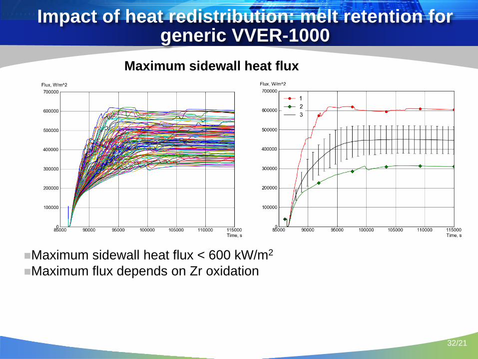
Impact of heat redistribution: melt retention for generic VVER-1000
Maximum sidewall heat flux < 600 kW/m2
Maximum flux depends on Zr oxidation
Maximum sidewall heat flux
32/21

15th Internationa
l Topical Meeting on
Nuclear Reactor The
In-vessel melt retention: thermal mechanics (HEFEST-M code)
Long-term strength model was validated on LHF (Sandia labs) experiments Creep parameters are considered
Temperature field and vessel melting – from previous simulation (highest flux)
130 code instances (0.95/0.99)
0( , , ) ( ) ( ) ( , )p p p py y tT d T E T f d Tσ ε σ ε= + +
( )( , ) ( )( )p Tpf d T B T d β=
Varied parameters
Varied parameter Range
B ± 20%
β ± 5%
Long-term strength parameter
± 30%
Filippov A.S., Drobyshevsky N.I., Strizhov V.Th., Simulation of Vessel-with-melt Deformation by SOCRAT/HEFEST Code, 17th Int. Conf. on Nucl. Eng., ICONE17, July 12-16, 2009,
Brussels, Belgium
33/21

In-vessel melt retention: thermal mechanics (HEFEST-M code)
After 200 000 s (more than 2 days) the residual thickness exceeds 3 cm.
Min Max Average 3.4 cm 6.1 cm 5.1 cm
What will happen in longer timespan?
Heat flux will decrease and: In metallic layer RPV thickness will
increase In oxide layer heat-insulating crust
will grow and T will decrease

Summary
Advanced CFD codes allow predictions of local flow characteristics Computation technique realized in the CONV3D was tested on HPC and showed effectiveness of algorithms for parallel computations Integrated best estimate multi-physics tools based on simplified description of processes can be used in combination with uncertainties evaluation (BEPU methoodology).
Related Documents


![UNITED STATES COURT OF INTERNATIONAL TRADE NSK LTD., NSK ...public].pdf Plaintiffs and Defendant-Intervenors NSK Ltd., NSK Corp., NSK Precision America, Inc. Barnes, ... covering a](https://static.cupdf.com/doc/110x72/5c4aa13793f3c34c55086977/united-states-court-of-international-trade-nsk-ltd-nsk-publicpdf-plaintiffs.jpg)


