High-frequency analysis of Earth gravity field models based on terrestrial gravity and GPS/levelling data: A case study in Greece

© 2015 T. D. Papanikolaou et al., licensee De Gruyter Open.This work is licensed under the Creative Commons Attribution-NonCommercial-NoDerivs 3.0 License.

J. Geod. Sci. 2015; 5:67–79

Research Article Open Access

T. D. Papanikolaou* and N. Papadopoulos

High-frequency analysis of Earth gravity fieldmodels based on terrestrial gravity andGPS/levelling data: a case study in GreeceDOI 10.1515/jogs-2015-0008Received January 12, 2015; accepted May 15, 2015

Abstract:Thepresent studyaimsat the validationof globalgravity field models through numerical investigation ingravity field functionals based on spherical harmonic syn-thesis of the geopotential models and the analysis of ter-restrial data. We examine gravity models produced ac-cording to the latest approaches for gravity field recoverybased on the principles of the Gravity field and steady-state Ocean Circulation Explorer (GOCE) and Gravity Re-covery And Climate Experiment (GRACE) satellite mis-sions. Furthermore, we evaluate the overall spectrum ofthe ultra-high degree combined gravity models EGM2008and EIGEN-6C3stat. The terrestrial data consist of gravityand collocated GPS/levelling data in the overall Hellenicregion. The software presented here implements the al-gorithm of spherical harmonic synthesis in a degree-wisecumulative sense. This approach may quantify the band-limited performance of the individual models by monitor-ing the degree-wise computed functionals against the ter-restrial data. The degree-wise analysis performed yieldsinsight in the short-wavelengths of the Earth gravity fieldas these are expressed by the high degree harmonics.

Keywords: GOCE; Gravity models; Gravimetry;GPS/levelling; Spherical harmonic synthesis

1 IntroductionThe role of global gravity field models is fundamental invarious research objectives such as precise orbit determi-nation of LEOs (Low Earth Orbiters), geoid modelling andgeophysical research. In such cases, the accuracy of the

*Corresponding Author: T. D. Papanikolaou: Department ofGravimetry, Hellenic Military Geographical Service, Greece, E-mail:[email protected], www.thomaspap.comN. Papadopoulos: Geodesy and Surveying Branch, Hellenic Mili-tary Geographical Service, Greece

gravity field functionals based on the global models e.g.gravity anomaly or geoid height, has a major effect in theoverall analysis and the results.

During the last decade, gravity fieldmappinghas beenbased on the innovative techniques that were introducedby the Gravity Recovery And Climate Experiment (GRACE)and Gravity field and steady-state Ocean Circulation Ex-plorer (GOCE) satellite missions (Tapley et al. 2004, ESA1999, Floberghagen et al. 2011). The new space-borne tech-niques of the two satellite gravitymissions have generatedextended numerical investigations as well as the evolu-tion of theoretical approaches in gravity field modelling.Therefore, a series of gravity fieldmodels according to var-iousmethodologies has beendemonstratedduring the lastfew years. The GRACEmission in-orbit since 2002 is imple-menting the concept of low-low satellite-to-satellite track-ing while the GOCE mission materialized the concept ofspace gravity gradiometry in the period 2009-2013. In ad-dition, the concept of a future satellite gravity mission isbeing studied (Loomis et al. 2012, Sheard et al. 2012, Panetet al. 2013, Elsaka et al. 2014) by considering the achieve-ments aswell as the limitations of themeasurementprinci-ples and the orbital design of the two aforementionedmis-sions. Thus, the validation of the gravity field models de-termined by the current adopted approaches is a criticalaspect in the satellite gravity missions’ performance.

The assessment of global gravity models may be in-vestigated by a variety of quality tests such as the anal-ysis of satellite orbits and terrestrial data (Förste et al.2008, Arabelos and Tscherning 2010, Tapley et al. 2005,Featherstone 2001, Lemoine et al. 1998, Perosanz et al.1997), space-borne data analysis (Hashemi Farahani et al.2013a, Papanikolaou and Tsoulis 2014) or even spectral as-sessment and error analysis of the harmonics coefficients(Tsoulis and Patlakis 2013, Baur et al. 2014).

The present study aims at the validation of currentgravity models through the numerical comparison be-tween the terrestrial data and the gravity field functionalscomputed through the procedure of spherical harmonicsynthesis of the geopotential models. We focus in the eval-

UnauthenticatedDownload Date | 7/1/15 1:59 PM

www.thomaspap.com

68 | T. D. Papanikolaou and N. Papadopoulos

uation of global gravity models that have been producedaccording to the current methodologies adopted in thegravity field recovery based on the principles of GOCEand GRACE satellite gravity missions. The satellite gravitymodels, that are analyzed here, are referred to approachessuch as the short-arc method (Mayer-Gürr 2006, Mayer-Gürr 2010), the celestial mechanics approach (Beutler etal. 2010), the acceleration approach (Ditmar et al. 2006,Hashemi Farahani et al. 2013b) and the three major meth-ods adopted in the frame of the European Space Agency(ESA) project GOCE High-level Processing Facility (Pail etal. 2011) i.e. the direct (Bruinsma et al. 2013), time-wise(Pail et al. 2010) and space-wise (Migliaccio et al. 2011) so-lutions of the Earth’s gravity field.

We examine the GOCE-based satellite gravity modelsthat may be distinguished in the GOCE-only models andthe models that have been extracted by optimum combi-nation of GOCE and GRACE data processing. In addition,we have elaborated state-of-the-art models compiled ex-clusively by GRACE observations.

Furthermore, we focus on evaluating the ultra-highdegree combined gravity models i.e. the EGM2008 (Pavliset al. 2012) and EIGEN-6C3stat models (Förste et al. 2013).These twomodels are analyzedhere in theirwhole spectralcontent which is expressed by the overall spherical har-monics range.

The terrestrial data consist of gravity andGPS/levelling measurements in the overall Hellenic re-gion. These data have been obtained from the database ofthe Hellenic Military Geographical Service (HMGS). Thedata have been derived in the frame of national projectsthat are described as follows.

Studies for the validation of GOCE-based gravity mod-els through terrestrial data over various geographical re-gions have been carried out by Gruber et al. (2011), Hirtet al. (2011), Šprlák et al. (2012), Voigt and Denker (2014),Rexer et al. (2014). An evaluation of global gravity mod-els over Greece can be found in Kotsakis and Katsambalos(2010), Vergos et al. (2012), etc.

The spherical harmonic synthesis for gravity fieldfunctionals is implemented here in a degree-wise cumu-lative sense. The algorithm of harmonic synthesis is re-peated for each individual degree and we monitor theresiduals of the terrestrial data to the computed valuesconsidering the global gravity models. Therefore, the pro-posed analysis schememay quantify the band-limited per-formance of the individual models.

The aforementioned degree-wise cumulative ap-proach has been previously applied for global gravitymodels validation through a scheme of dynamic orbitanalysis by Papanikolaou and Tsoulis (2014).

2 Theoretical backgroundThe basic tool for the synthetic evaluation of the Earth’sgravity functionals is the expression of the gravitationalpotential V in terms of a spherical harmonic expansion(Heiskanen and Moritz 1967)

V = GMr ×∞∑︁n=0

(︁aer

)︁n n∑︁m=0

P̄nm (cos θ)(︀C̄nm cos (mλ) + S̄nm sin (mλ)

)︀(1)

where GM is the product between the constant of gravita-tion G and the total Earth’smassM, ae is the equatorial ra-dius, (r, θ, λ) are the spherical coordinates of the computa-tion point, C̄nm and S̄nm are the normalized spherical har-monic coefficients that are provided by the gravity model,and P̄nm are thenormalized associated Legendre functionswith n and m denoting degree and order, respectively.

The Legendre functions are described in several text-books e.g. Hobson (1931), Abramowitz and Stegun (1965),Heiskanen and Moritz (1967). The numerical stability andaccuracy of the normalized associated Legendre functionspresented in Eq. 1 is a critical computing problem (Bosch2000, Claessens 2005, Montenbruck and Gill 2000), espe-cially in the case of very high degree and order (Wittweret al. 2008, Holmes and Featherstone 2002). The numer-ical stability is treated here by implementing appropriaterecurrence relations into our source code that are recom-mended for this purpose (Montenbruck and Gill 2000).

The geoid undulation is given by the following equa-tion (Heiskanen and Moritz 1967)

N (φ, λ) = ζp (φ, λ, r) + ∆gB�̄�H (2)

where ∆gB is theBouger gravity anomaly,H is the orthome-tric height, p denotes the computation point with spheri-cal coordinates (φ, λ, r) and �̄� is the average value of thenormal gravity along the normal plumb line between tel-luroid and ellipsoid.

The height anomaly ζp, which expresses the distancebetween the computation point and the telluroid surface,is computed according to Bruns’ formula

ζp (φ, λ, r) = Tp − (W0 − U0)𝛾p

(3)

or equivalently

ζp (φ, λ, r) = GM − GM0r𝛾p

− W0 − U0𝛾p

+ GMr𝛾p×

∞∑︁n=2

(︁aer

)︁n n∑︁m=0

P̄nm (cos θ)(︀dC̄nm cos (mλ) + S̄nm sin (mλ)

)︀(4)


High-frequency analysis of Earth gravity field models | 69

where Tp is the disturbing potential, 𝛾p is the value of nor-mal gravity at the point p and dC̄nm are obtained from thedifferences between C̄nm and C̄enm(J2n ,m = 0) i.e. the co-efficients of the zonal harmonics of the normal gravita-tional potential. In the present computations we considerthe zonal harmonic coefficients for degree values equal to2, 4, 6 and 8.

TheW0 and U0 refer to the gravity potential of the ac-tual and the normal gravity field respectively, while GM0is the geocentric gravitational constant of the normal grav-ity field. In the present study, we consider the values ofGM0 andU0with respect to theGeodetic Reference System1980 (GRS80)which are given byMoritz (2000) and theW0value as it has been adopted by the International Earth Ro-tation and Reference Systems Service (IERS) Conventions(Petit and Luzum 2010). Moreover, our computations withrespect to the WGS84 (World Geodetic System 1984) haveshown small differences at sub-mm level in terms of geoidheight.

The first term of Eq. 3)

N0 =GM − GM0

r𝛾p− W0 − U0

𝛾p(5)

is known in the literature as the zero-degree term (Heiska-nen and Moritz 1967).

The zero-degree term has been computed, within thestudy region, equal to −0.4422 meters with respect toGRS80.

Eq. 4 requires further analysis, prior to its implemen-tation, in case where the ellipsoidal height of the compu-tation point is not known as it is discussed in Rapp (1997).The steps for the additional reduction are well describedby Rapp (1997) and Lemoine et al. (1998).

The Bouger gravity anomaly in Eq. 2 is obtainedthrough the following reduction of the free-air gravityanomaly

∆gB = ∆gFA − 0.1119H. (6)

The free-air gravity anomaly ∆gFA is computed in terms ofspherical harmonic expansion by the following equation

∆gFA =GMr2

∞∑︁n=2

(n − 1)(︁aer

)︁nn∑︁

m=0P̄nm (cos θ)

(︀dC̄nm cos (mλ) + S̄nm sin (mλ)

)︀. (7)

The equations presented in this section, which are ex-pressed in spherical harmonic expansion series, aretreated here in a degree-wise cumulative sense. We repeatthe computational procedure for each degree and the ex-pansion series are formed by using all previous harmoniccoefficients up to that specific degree. This approach may

reveal band-limited areas of the models’ harmonics andrepresents the dynamic contribution of the coefficients be-longing to an individual degree.

The gravity field models usually provide the series ofthe spherical harmonic coefficients C̄nm and S̄nm referringin the tide free system or “conventional tide free system” ina rigorous sense. This term assumes that the effects of allthe constituents of the solid Earth and ocean tides havebeen removed. However, the gravity models may be re-ferred in the “zero tide” systemwhich contains the perma-nent part of the tides. In the current analysis, in order tobe consistent with all models, the zero tide gravity modelsare converted in the tide free system. In this case, the per-manent part of the tides is removed prior to the analysisaccording to the Earth tides modelling as it is extensivelydescribed in the IERSConventions (Petit and Luzum2010).For this purpose, we apply the required correction to theC̄20 coefficient that enters Eq. 1, 4 and 7

C̄tf20 = C̄zt20 − ∆C̄perm20 (8)

where ∆C̄perm20 is the correction, C̄zt20 and C̄tf20 are the zero-tide and tide-free coefficients correspondingly.

The respective correction is computed by taking in ac-count the adopted formula by the IERS Conventions (Petitand Luzum 2010, Eq. 6.14)

∆C̄perm20 =(︁4.4228 × 10−8

)︁(−0.31460) k20 (9)

with k20 being a nominal Love number equal to 0.30190.

3 DataThe terrestrial data used in the present analysis havebeen provided by the Hellenic Military Geographical Ser-vice (HMGS) which established the national gravity, lev-elling and triangulation networks. Since the last decade,HMGS has maintained these networks by performing GPSand gravity surveys all over the Hellenic region. Here, webriefly describe the projects that have been performed andprovided thegravity andGPSdataused in the current anal-ysis. Overall, the presented terrestrial data consist of 9658gravity data points and 3293 co-located GPS/Levellingpoints.

3.1 GPS data

HMGS initialized the HEllenic GPS NETwork 2002 (HEG-NET2002) project (Anagnostou 2007) in 2000. In the frameof this project, a national GPS network was established as



it is illustrated in Fig. 1. The GPSmeasurements performedduring 2000 and 2001 while the data was processed us-ing Bernese GPS software (Dach et al. 2007). Themeasure-ments are referred to benchmarks of the national trian-gulation network. In particular, the HEGNET2002 networkcomprises the following data points that form the 1st ordernetwork.

Figure 1: HEGNET2002 network referring in 1st order.

– the permanent GPS station DIONYSOS, defined asthe network’s reference station, which is consid-ered in the InternationalGNSSService (IGS) network(Dow et al. 2009).

– 28 points at benchmarks of the national triangula-tion network that were adjusted as reference points.

– 201 points at benchmarks of the national triangula-tion network

– 9 points at tide gauges that have contributed in theSELF (Sea Level Fluctuations) project (Zerbini et al.1996).

– 5 points at benchmarks where Satellite Laser Rang-ing (SLR) baselineshavebeenmeasured in the frameof the WEGENER (Working group of European Geo-scientists for the Establishment of Networks forEarth-science Research) project (Wilson 1996).

In 2004,HMGS initializedGPS and gravity surveys in orderto cover the overall Hellenic region with spatial distribu-tion of 8 points per 25 km × 25 kmapproximately. Since thisproject is still in progress, in the present analysis we usea part from these data that refers to the region of CentralGreece and comprise 660 gravity and GPS data points thathave been collected by field campaigns from 2004-2007.

In addition, we use here GPS data that have beencollected in the frame of the Hellenic Positioning Sys-tem (HEPOS) project (Gianniou 2010) which has been or-

ganized by the National Cadastre and Mapping Agency.These data consist of 2431 GPS points at benchmarks of thenational triangulation network.

3.2 Levelling data

The Hellenic Vertical Datumwas established by HMGS ac-cording to a Helmert-type orthometric height system. Theorthometric heights of the national leveling network referto one origin i.e. the tide gauge station placed at the Pi-raeus harbor. The measurements at this station during theperiod 1933-1978 were considered exclusively for the esti-mation of the local mean sea level (Takos 1989). The or-thometric heights of the national triangulation network’sbenchmarks were estimated through spirit and trigono-metric leveling tieswith the national leveling network. Nu-merical investigations on the assessment of the Hellenicvertical datum have been carried out by Kotsakis et al.(2012), Grigoriadis et al. (2014) for the case of the Hellenicislands and Andritsanos et al. (2014), Tziavos et al. (2012)for selected regions in Central and Northen Greece.

Since the orthometric heights were estimated at thebenchmarks of the triangulation network, the GPS obser-vations performed at these points may yield geoid undula-tions with respect to the GPS/leveling technique

NGPS−lev = h − H (10)

where H denotes the orthometric height, h is the el-lipsoidal height obtained by the GPS observations andNGPS−lev is the computed geoid undulation.

3.3 Gravity data

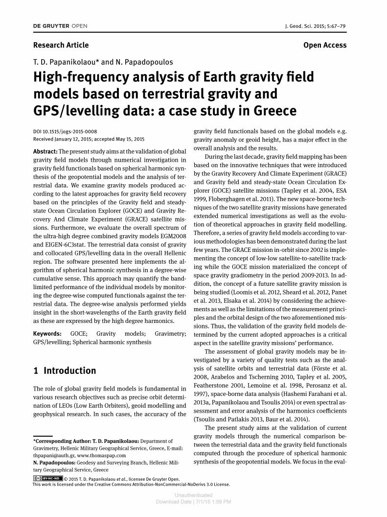
The national gravity network consists of 8 stations of zeroorder, 50 stations of 1st order and 88 stations of 2nd order,as shown in Fig. 2. The network is referred to the Inter-national Gravity Standardization Net 1971 (IGSN71) grav-ity datum (Morelli et al. 1974) through one reference sta-tion, i.e. the National Gravity Station located in Athens.The reference station has been connected through loopswith gravity stations in Rome, Frankfurt and Addis Ababawhich are part of the IGSN71 network.

In the frame of the aforementioned national field cam-paigns, gravity measurements were collected in parallelwith the GPS survey asmentioned in Section 3.2. Themea-surements were observed by the relative gravimeters La-Coste & Romberg G730, G496, G63 and D107. Gravimetryobservations were carried out by forming loops where theinitial and final points have been selected as points of the



gravity network. These data are provided as gravity valuesreferred in the IGSN71 system.

Moreover, a set of 8998 gravity data points has beenobtained from the database of the HMGS. These data werederived from past gravimetry surveys that were not per-formed at benchmarks of the triangulation/leveling net-work and the corresponding accuracy of the positioningand levelling is lower compared to the rest of the gravime-try field surveys. Therefore, this data set is applied in thepresent analysis separately in order to avoid systematic ef-fects that may come from the reference system.

Figure 2: HMGS gravity network.

4 Computing and resultsIn the frame of the present computations, the GRAVsynthsoftware for spherical harmonic synthesis has been devel-oped byPapanikolaou (2013)with a part of the source codeprovided by Papanikolaou (2012). Our source code imple-ments the harmonic synthesis for gravity field function-als i.e. the gravity anomaly, the height anomaly and thegeoid undulation, according to the mathematical formu-las described in Section 2. The computations run in a stan-dard PCwhere the corresponding CPU time varies at about4 hours for a data set of 9000 computation points basedon harmonics series expansion with maximum degree upto 2000. Preliminary results of the current work have beenreported in Papanikolaou and Papadopoulos (2013).

An accuracy assessment of our source code has beenperformed through comparison with the HARMONIC_SYNTH_ WGS84 software (Holmes and Pavlis 2008). Thenumerical comparison has led to differences in geoidheights that vary from 10−4 to 10−1 meters for theGPS/levelling data set of the 3293 computation points. It

should be remarked that these discrepancies are partlyaffected by systematic differences in the adopted zero-degree term and the heights data sources.

Moreover, we have applied comparisons betweenGRAVsynth and the web-based calculation service(icgem.gfz-potsdam.de/ICGEM) of the International Cen-tre of Global Earth Models (ICGEM). The numerical dif-ferences obtained for 65341 points in global scale, haveyielded RMS values of 2 cm and 0.18 mgal in terms ofgeoid and free-air gravity anomalies, respectively.

The gravity field models that have been elaboratedhere are listed in Table 1 together with the type of dataprocessed during the models’ determination. The modelsare provided by the International Centre for Global EarthModels (ICGEM) according to the format of the ICGEM(Barthelmes and Förste 2011). We have analyzed the high-degree combined gravity models EGM2008 (Pavlis et al.2012) and EIGEN-6C3stat (Förste et al. 2013), which is thelatest available version of the European Improved Gravitymodel of the Earth by New techniques (EIGEN) series. Inaddition, we have considered satellite-only gravity mod-els such as the latest releases of the GOCE models basedon the direct (Bruinsma et al. 2013), time-wise (Pail et al.2010) and space-wise (Migliaccio et al. 2011) approaches,the ITG-Goce02 (Schall et al. 2014) and JYY_GOCE04S (Yiet al. 2013) which are GOCE-only solutions, the DGM-1S(Hashemi Farahani et al. 2013b) and GOCO-03S (Mayer-Gürr et al. 2012)which are combined satellite-onlymodels,the GGM05S (Tapley et al. 2013), AIUB-GRACE03S (Jäggiet al. 2012) and ITG-Grace2010s (Mayer-Gürr et al. 2010)which have been determined exclusively by GRACE obser-vations analysis.

We have used the two latest ESA releases of the GOCEgravitymodels (Pail et al. 2011) i.e. the 4th and 5th releases,for the time-wise and direct approaches as well as the lat-est model of the space-wise approach that comes from the2nd release. In the following, we refer to these models byusing the terms GOCE-DIR-Rx, GOCE-TIM-Rx and GOCE-SPW-Rx respectively for the three approaches and Rx de-notes the particular release e.g. R5, R4, R2.

The latest GOCE release of time-wise and direct solu-tions i.e. the 5th release (R5), has taken into account theentire data from the satellite mission’s lifetime includingthe last low-orbit phase (GFCT2014).During this last phasethe orbital altitude has been decreased from the routinealtitude of 260 km to 229 km. Therefore, the sensitivity ofthe GOCE observations analysis due to the Earth’s gravita-tional perturbations has been increased. The strength ofthis sensitivity is pronounced in the present computationsthrough the relative comparison of the results based on theR4 and R5 GOCE models.



Table 1: Satellite data and maximum degree of the used Earth gravity models.

Gravity Field Models DegreeData type used (x: yes / -: no)

Gravity Altimetry Satellite trackingEGM2008 2190 x x GRACE

EIGEN-6C3stat 1949 x x GOCE, GRACE, LAGEOSGO_ CONS_ GCF_ 2_ TIM_ R5 280 - - GOCEGO_ CONS_ GCF_ 2_ DIR_ R5 300 - - GOCE, GRACE, LAGEOSGO_ CONS_ GCF_ 2_ TIM_ R4 250 - - GOCEGO_ CONS_ GCF_ 2_ DIR_ R4 260 - - GOCE, GRACE, LAGEOSGO_ CONS_ GCF_ 2_ SPW_ R2 240 - - GOCE

ITG-Goce02 240 - - GOCEJYY_ GOCE04S 230 - - GOCE

DGM-1S 250 - - GOCE, GRACEGOCO-03S 250 - - GOCE, GRACE, CHAMP, SLRGGM05S 160 - - GRACE

AIUB-GRACE03S 160 - - GRACEITG-Grace2010s 180 - - GRACE

The ITG-Goce02, GGM05S and ITG-Grace2010smodelsrefer to the zero tide system and thus, we add the requiredcorrection in order to convert them to the tide free systemaccording to the formula discussed in Section 2 (Eq. 9 and??).

According to the procedure of the spherical harmonicsynthesis as presented in the previous sections, we havecomputed geoid undulations and free-air gravity anoma-lies at the data points presented in Section 3. The compar-ison between the values from the gravity models and theterrestrial gravity andGPS/levelingdata,maybedescribedby the following equations

∆N = N lev − NGGM = (h − H) − NGGM (11)

∆Dg = Dgfagrav − DgfaGGM (12)

where NGGM is the geoid undulation computed by theglobal gravity model, H denotes the orthometric height,h refers to the ellipsoidal height obtained by the GPS ob-servations and NGPS−lev denotes the geoid height by theGPS/levelling technique.

The terms Dgfagrav and DgfaGGM denote the free-air grav-ity anomaly derived by the gravity data and the computedvalues based on the gravity models respectively.

The computations have been carried out for the threedata sets described in Section 3 i.e. the 3293 GPS/levelingand 8998 gravity data points in the overall Hellenic regionaswell as the 660 gravity data points in the Central Greece.The two gravity data sets are applied individually in thecomputations since the corresponding campaign surveys

were not performed according to common standards andthus, systematic differences may occur.

The numerical comparison between the gravity mod-els and the terrestrial data has also been considered as avaluable tool in order to detect outliers. We have removedpart of the data i.e. 45 points, by setting limits inmaximumdifference as outliers’ limits i.e. 300 mgal and 5 meters forthe differences in gravity anomalies and geoid heights re-spectively.

The numerical comparison is expressed by represen-tative statistical quantities such as the root mean square(RMS), standard deviation, mean, maximum and mini-mum values. The respective results are shown in Tables 2and 3.

In general, the gravity models derived from the com-bination of the GOCE and GRACE data has yielded a bet-ter fit according to the residuals of the gravity and theGPS/levelling data. The comparison among the GOCE R5and R4 released models reveal the contribution of theadditional GOCE data during the last phase of low-orbit(GFCT 2014). The lower orbital altitude provided sensitiv-ity to the estimation of additional spherical harmonic co-efficients at higher degree. Therefore, the R5 models aregiven at higher degree. This overall improvement has beencaptured in the present computations at the level cm- and0.5 mgal level based on the GPS/levelling and gravity dataresiduals, respectively (Tables 2 and 3).

The space-wisemodel (GOCE-SPW-R2) presents higherresiduals than the other GOCE-based models but leads tobetter results than the GRACE-only models. Nevertheless,the space-wise model has yielded low performance in the



Table 2: Statistics of the comparison between GPS/levelling data and geoid heights based on global gravity models after the estimation ofa constant bias. Data refer to a set of 3293 data points over the Hellenic region. Maximum degree of its model is considered. Unit is meters.

Gravity Field Models RMS bias Min MaxEGM2008 0.278 0.692 −4.233 3.843

EIGEN-6C3stat 0.273 0.690 −4.301 3.930GOCE-DIR-R5 0.552 0.818 −4.439 3.916GOCE-DIR-R4 0.568 0.823 −4.455 3.831GOCE-TIM-R5 0.567 0.813 −4.465 3.871GOCE-TIM-R4 0.574 0.826 −4.591 3.876GOCE-SPW-R2 0.643 0.862 −4.601 3.962ITG-Goce02 0.612 0.8431 −4.4938 3.7642

JYY_ GOCE04S 0.609 0.8507 −4.5231 3.9242DGM-1S 0.622 0.841 −4.634 3.936GOCO-03S 0.604 0.841 −4.482 3.883GGM05S 0.900 0.9124 −5.5884 3.9872

AIUB-GRACE03S 0.759 0.8904 −4.4836 2.7196ITG-Grace2010s 0.759 0.911 −5.115 3.446

Table 3: Statistics of the comparison between gravity anomalies based on global gravity models and a data set of 8998 free-air gravityanomalies over Greece. Maximum degree of its model is considered. Unit is mgal.

Gravity Field Models RMS σ Mean Min MaxEGM2008 21.96 20.56 7.70 −192.26 288.43

EIGEN-6C3stat 22.39 21.08 7.55 −186.16 285.37GOCE-DIR-R5 44.94 40.81 18.82 −206.84 270.10GOCE-DIR-R4 45.76 41.44 19.39 −204.12 260.35GOCE-TIM-R5 45.16 41.09 18.75 −204.51 265.62GOCE-TIM-R4 45.50 41.12 19.49 −199.61 263.43GOCE-SPW-R2 48.69 43.46 21.96 −189.31 255.92ITG-Goce02 47.16 42.54 20.37 −192.73 259.25

JYY_ GOCE04S 46.72 42.06 20.33 −193.19 257.16DGM-1S 47.17 42.72 20.01 −192.15 260.56GOCO-03S 46.70 42.13 20.16 −190.19 253.36GGM05S 53.41 47.89 23.65 −186.82 254.50

AIUB-GRACE03S 51.87 46.27 23.45 −171.75 257.57ITG-Grace2010s 51.89 46.15 23.71 −178.93 248.88

analysis of the GRACE satellites orbit and inter-satelliteK-band ranging (KBR) observations (Papanikolaou andTsoulis 2014).

The analysis of the GPS/levelling data reveals system-atic errors that canbe absorbed through the estimationof aconstant bias (Table 2). The bias is estimated based on theleast-squares method according to the equations of obser-vations as follows:

N lev = NGGM + bias + v. (13)

where v denotes the random errors.

The estimated bias varies from 70 to 90 cm for vari-ous geopotential models shown in Table 2. The bias’ orderof magnitude may imply the presence of systematic differ-ences in the level surface of the vertical reference frame.Asmentioned in Section 3.2, the present orthometric heightsrefer to the Hellenic Vertical Datum. The datum was es-tablished according to the local mean level estimated bythe tide gauge station at the Piraeus harbor. Therefore, thebias may be interpreted as a level difference between thelocal mean sea level and the geoid approximated througha global gravity model. According to the present computa-tions, the level of the heights has been found to be about



69 cm lower than the global geoid with respect to the high-degree gravity models.

However, further analysis is required formodelling theresiduals between these two level surfaces which may in-clude additional parameters for treating tilts andother sys-tematic errors in heights systems. By estimating additionalparameters the fitting of the global gravity models mayimproved in terms of geoid residuals. On the other hand,such parametric models may absorb part of the errors ofthe global gravity models. Since the scope of this study isthe evaluation of the gravity models, we estimate only oneconstant bias parameter.

In particular, the bias is estimated to be 75 cm approx-imately for considering only the GPS/leveling data in Cen-tral Greece while in the overall Hellenic region the bias es-timation is equal to 69 cm (Table 1). These values are validfor EGM2008 and EIGEN-6Cstat models up to their maxi-mum degree. This small discrepancy in bias estimation isjustified due to systematic differences in the Hellenic ver-tical datum among the mainland and islands (Kotsakis etal. 2012, Grigoriadis et al. 2014). Our bias estimation is inclose agreement with Tziavos et al. (2012) who obtained amean value of 75 cm for EGM2008 based on GPS/levellingdata in the region of Thessaloniki in Northern Greece. Nev-ertheless, there are significant differences in comparisonwith the bias estimated byKotsakis andKatsmbalos (2010)and Vergos et al. (2014).

The degree-wise cumulative analysis, as it has beendiscussed in Section 2, has been implemented for selectedsatellite-only gravity models as well as the EGM2008 andEIGEN-6C3stat combined gravity models. The degree in-terval between the sequential iterations of the harmonicssynthesis algorithm has been set as 1. The data used re-fer to 660 gravity and GPS/levelling computation points inCentral Greece. The corresponding results are illustratedin Fig. 3 to 8. The corresponding satellite-onlymodels havebeen distinguished in the following selected groups forthe application of the degree-wise cumulative analysis i.e.the models based on the time-wise, space-wise and directapproaches (Pail et al. 2011), the GOCE-only models, theGRACE-onlymodels and the satellite gravitymodels basedon the combination of GOCE and GRACE data analysis.

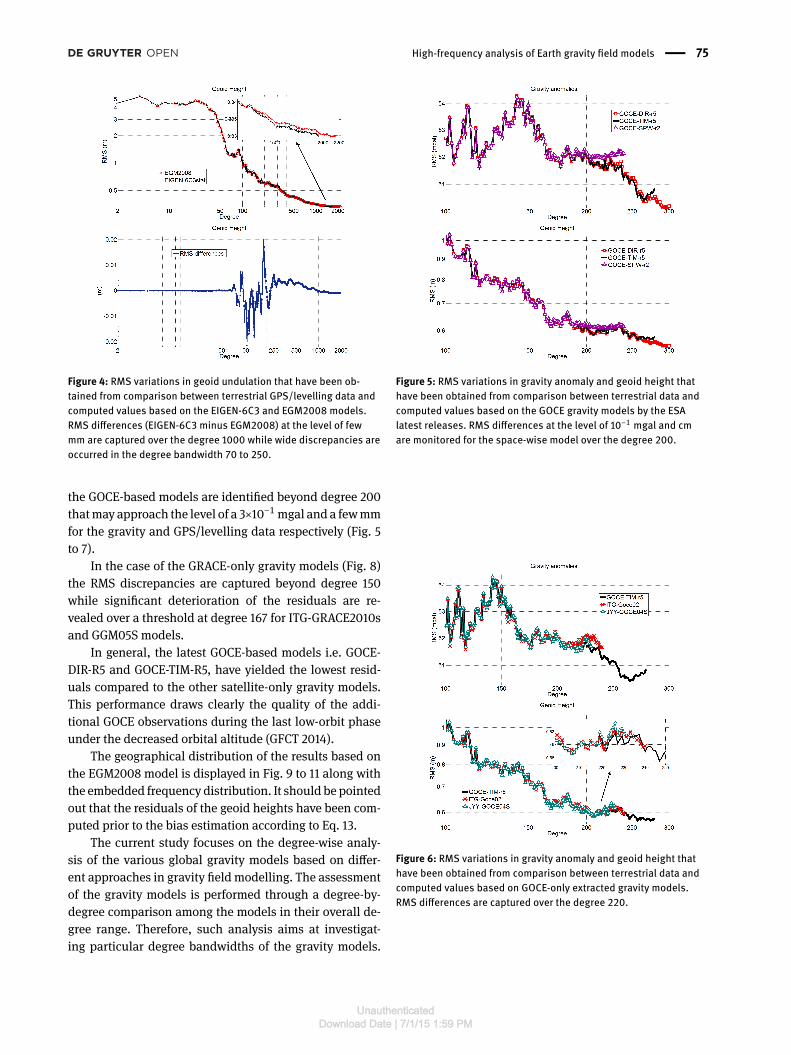
The two high-degree combined gravity models havebeen analyzed according to the degree-wise cumulativeapproach over the full degree range (Fig. 3 and 4). Thisanalysis has captured the small RMS variations as a func-tion of the truncated degree and may yield insights intothe different spectral ranges of the ultra-high degree grav-ity models. The numerical comparison detects discrepan-cies over the degree 1000 that vary at the level of a fewmmand 10−1 mgal in terms of RMS differences for the geoid

height and gravity anomaly respectively.Moreover, the dif-ferences of the corresponding RMS values present widevariations in the degree bandwidth from70 to 250 thatmayreach the level of a few cm and 0.3 mgal for geoid heightand gravity anomaly respectively. Beyond degree 250, theRMS differences are getting smoother and reduced. Thisbehavior implies the impact of incorporating the GOCEdata incorporation in the EIGEN-6C3stat model. In partic-ular, this reflects the major effect of the space-borne grav-ity gradiometry data that have been analyzed for gravityfield modelling in the degree range from 0 to 235 (Försteet al. 2013). Furthermore, the threshold at degree 70 is af-fected by the combination algorithm for the various dataincluded in the gravity field solutions of the EIGEN series(Förste et al. 2008). We should also mention that the satel-lite observations underlying the two combined models re-fer to the LAGEOS, GRACE and GOCE data analysis in thecase of the EIGEN-6C3stat (Förste et al. 2013)while the ITG-GRACE03s model (Mayer-Gürr 2007), which is a GRACE-onlymodel, has been incorporated in the case of EGM2008(Pavlis et al. 2012).

Figure 3: RMS variations in free-air gravity anomaly that have beenobtained from comparison between terrestrial gravity data and com-puted values based on the EIGEN-6C3 and EGM2008 models. RMSdifferences (EIGEN-6C3 minus EGM2008) at the level of 10−1 mgalare monitored over the degree 1000 while wide discrepancies areoccurred in the degree bandwidth 70 to 250.

In the case of the satellite-only gravity models, thedegree-wise cumulative analysis has been oriented in thedegree range from 100 up to the maximum degree of itsindividual model (Fig. 5 to 8). The differences in the mon-itored residuals, by means of the RMS differences, among



Figure 4: RMS variations in geoid undulation that have been ob-tained from comparison between terrestrial GPS/levelling data andcomputed values based on the EIGEN-6C3 and EGM2008 models.RMS differences (EIGEN-6C3 minus EGM2008) at the level of fewmm are captured over the degree 1000 while wide discrepancies areoccurred in the degree bandwidth 70 to 250.

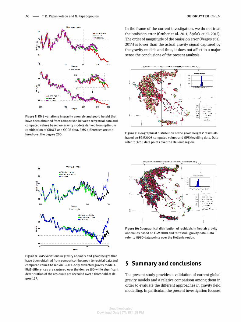
the GOCE-based models are identified beyond degree 200thatmay approach the level of a 3×10−1mgal and a fewmmfor the gravity and GPS/levelling data respectively (Fig. 5to 7).

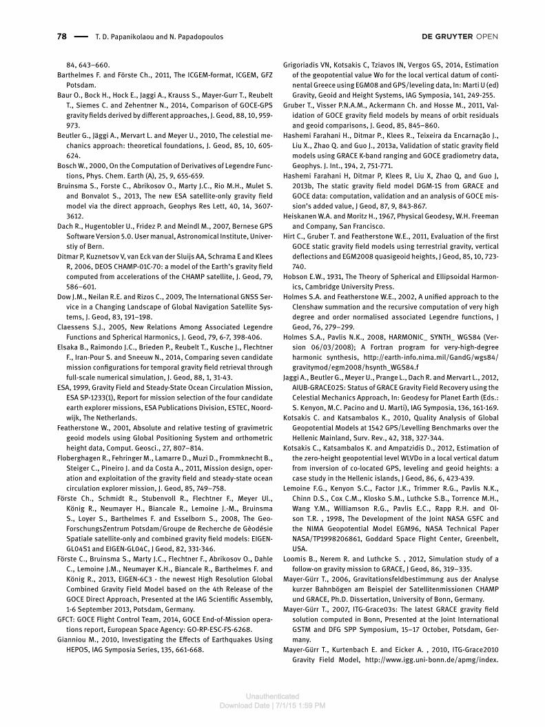
In the case of the GRACE-only gravity models (Fig. 8)the RMS discrepancies are captured beyond degree 150while significant deterioration of the residuals are re-vealed over a threshold at degree 167 for ITG-GRACE2010sand GGM05S models.

In general, the latest GOCE-based models i.e. GOCE-DIR-R5 and GOCE-TIM-R5, have yielded the lowest resid-uals compared to the other satellite-only gravity models.This performance draws clearly the quality of the addi-tional GOCE observations during the last low-orbit phaseunder the decreased orbital altitude (GFCT 2014).

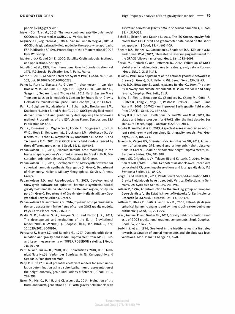
The geographical distribution of the results based onthe EGM2008 model is displayed in Fig. 9 to 11 along withthe embedded frequency distribution. It should be pointedout that the residuals of the geoid heights have been com-puted prior to the bias estimation according to Eq. 13.

The current study focuses on the degree-wise analy-sis of the various global gravity models based on differ-ent approaches in gravity field modelling. The assessmentof the gravity models is performed through a degree-by-degree comparison among the models in their overall de-gree range. Therefore, such analysis aims at investigat-ing particular degree bandwidths of the gravity models.

Figure 5: RMS variations in gravity anomaly and geoid height thathave been obtained from comparison between terrestrial data andcomputed values based on the GOCE gravity models by the ESAlatest releases. RMS differences at the level of 10−1 mgal and cmare monitored for the space-wise model over the degree 200.

Figure 6: RMS variations in gravity anomaly and geoid height thathave been obtained from comparison between terrestrial data andcomputed values based on GOCE-only extracted gravity models.RMS differences are captured over the degree 220.



Figure 7: RMS variations in gravity anomaly and geoid height thathave been obtained from comparison between terrestrial data andcomputed values based on gravity models derived from optimumcombination of GRACE and GOCE data. RMS differences are cap-tured over the degree 200.

Figure 8: RMS variations in gravity anomaly and geoid height thathave been obtained from comparison between terrestrial data andcomputed values based on GRACE-only extracted gravity models.RMS differences are captured over the degree 150 while significantdeterioration of the residuals are revealed over a threshold at de-gree 167.

In the frame of the current investigation, we do not treatthe omission error (Gruber et al. 2011, Sprlak et al. 2012).The order of magnitude of the omission error (Vergos et al.2014) is lower than the actual gravity signal captured bythe gravity models and thus, it does not affect in a majorsense the conclusions of the present analysis.

Figure 9: Geographical distribution of the geoid heights’ residualsbased on EGM2008 computed values and GPS/levelling data. Datarefer to 3268 data points over the Hellenic region.

Figure 10: Geographical distribution of residuals in free-air gravityanomalies based on EGM2008 and terrestrial gravity data. Datarefer to 8980 data points over the Hellenic region.

5 Summary and conclusionsThe present study provides a validation of current globalgravity models and a relative comparison among them inorder to evaluate the different approaches in gravity fieldmodelling. In particular, the present investigation focuses



Figure 11: Geographical distribution of residuals between free-airgravity anomalies based on EGM2008 and terrestrial gravity dataover 660 points in the Central Greece.

on the assessment of the GOCE-based gravity models forcapturing the contribution of the latest satellite gravitymission in Earth’s gravity field recovery.

We have implemented a computing procedure forspherical harmonic synthesis in a degree-wise cumulativesense. Based on such approach, we aim at quantifying theband-limited performance of the individual gravity mod-els and detecting degree bandwidths and thresholds thatreveal particular characteristics of the Earth gravity fieldsolutions. We have been monitoring the residuals of thedegree-wise computed gravity field functionals against theterrestrial data and record the variations of the RMS as afunction of the harmonics degree.

We applied the degree-wise approach to the latestGOCE-based satellite gravitymodels aswell as to the ultra-high degree combined models. The proposed analysis re-veals specific degrees within the models where signifi-cant discrepancies are occurring. This approach has beendemonstrated as a valuable tool in the assessment of thegravity models over the harmonics range even to high de-grees beyond 2000.

In general, the combination of GRACE and GOCE dataanalysis led to significant improvement in the Earth’sgravity field modelling. This is quite pronounced in thecomparison of the GOCE-GRACE satellite gravity modelsagainst the state-of-the-art GRACE-only models.

The current analysis is oriented to the high frequen-cies of the Earth’s gravity field as these are expressedby the higher degrees of the geopotential models. Thecomparison among the ultra-high degree gravity modelsEGM2008 and EIGEN-6C3stat, demonstrates that the sec-ondmodelwhichhas includedGOCEobservations leads toslightly better results in terms of the data residuals withinthe study region. This low improvement is better out-

lined in harmonics degrees higher than 1000. Moreover,a threshold in degrees around 200 has shown detectabledifferences in the different approaches of the GOCE-basedgravity models while a degree threshold equal to 167 hasrevealed significant deterioration of the GRACE-only mod-els’ performance.

The validation procedure is carried out throughthe numerical comparison between computed gravityfield functionals and terrestrial data i.e. gravity andGPS/levelling data over the Hellenic region. Therefore thecurrent analysis exhibit the fitting level of the current grav-itymodels in Greece based on the latest data sets that havebeen collected in national gravity and GPS surveys duringthe last decade.

Furthermore, the terrestrial gravity data have beenfound to be sensitive as an evaluation test even to thehigher degree harmonics. This is justified due to the ef-fect of the Earth gravity field frequencies in the mea-sured gravity signal by the gravimeters. Vice versa, thehigh-degree combined gravity models e.g. EGM2008 andEIGEN-6C3stat, may define a valuable tool for the detec-tion of significant errors in the terrestrial data and thus, re-move them as outliers. Even further, the high-degreemod-els yield geoid undulation residuals of the GPS/levellingdata that may reveal systematic errors of the local heightsystem and the adopted mean sea level. In particular, ithas been found according to the current analysis that thelevel of the used orhtometric heights, based on the meansea level of the study region, has been estimated to belower by about 69 cm than the geoid approximated by theEGM2008 or EIGEN-6C3stat gravity field models.

Acknowledgement: The authors acknowledge the Inter-national Centre for Global Earth Models for providing theglobal gravity field models and the National Cadastre andMapping Agency of Greece for providing the GPS data.

ReferencesAbramowitz M. and Stegun I. A., 1965, Handbook of Mathematical

Functions, Dover, New York.Anagnostou E., 2007, National Report of Greece to EUREF 2007, EUREF

Symposium Proceedings, 6-9 June 2007, London, UK.Andritsanos V.D., Vergos G.S., Grigoriadis V.N., Pagounis V. and Tzi-

avos I.N. , 2014, Spectral characteristics of the Hellenic verti-cal network - Validation over Central and Northern Greece usingGOCE/GRACE global geopotential models, Geophys. Res. Abstr.,Vol. 16, EGU2014-1223.

Arabelos D. and Tscherning C.C., 2010, A comparison of recent Earthgravitational models with emphasis on their contribution in refin-ing the gravity and geoid at continental or regional scale, J. Geod,



84, 643–660.Barthelmes F. and Förste Ch., 2011, The ICGEM-format, ICGEM, GFZ

Potsdam.Baur O., Bock H., Hock E., Jaggi A., Krauss S., Mayer-Gurr T., Reubelt

T., Siemes C. and Zehentner N., 2014, Comparison of GOCE-GPSgravity fieldsderivedbydifferent approaches, J. Geod, 88, 10, 959-973.

Beutler G., Jäggi A., Mervart L. and Meyer U., 2010, The celestial me-chanics approach: theoretical foundations, J. Geod, 85, 10, 605-624.

BoschW., 2000, On the Computation of Derivatives of Legendre Func-tions, Phys. Chem. Earth (A), 25, 9, 655-659.

Bruinsma S., Forste C., Abrikosov O., Marty J.C., Rio M.H., Mulet S.and Bonvalot S., 2013, The new ESA satellite-only gravity fieldmodel via the direct approach, Geophys Res Lett, 40, 14, 3607-3612.

Dach R., Hugentobler U., Fridez P. and Meindl M., 2007, Bernese GPSSoftwareVersion 5.0. Usermanual, Astronomical Institute, Univer-stiy of Bern.

Ditmar P, Kuznetsov V, van Eck van der Sluijs AA, Schrama E and KleesR, 2006, DEOS CHAMP-01C-70: a model of the Earth’s gravity fieldcomputed from accelerations of the CHAMP satellite, J. Geod, 79,586–601.

Dow J.M., Neilan R.E. and Rizos C., 2009, The International GNSS Ser-vice in a Changing Landscape of Global Navigation Satellite Sys-tems, J. Geod, 83, 191–198.

Claessens S.J., 2005, New Relations Among Associated LegendreFunctions and Spherical Harmonics, J. Geod, 79, 6-7, 398-406.

Elsaka B., Raimondo J.C., Brieden P., Reubelt T., Kusche J., FlechtnerF., Iran-Pour S. and Sneeuw N., 2014, Comparing seven candidatemission configurations for temporal gravity field retrieval throughfull-scale numerical simulation, J. Geod, 88, 1, 31-43.

ESA, 1999, Gravity Field and Steady-State Ocean Circulation Mission,ESA SP-1233(1), Report for mission selection of the four candidateearth explorer missions, ESA Publications Division, ESTEC, Noord-wijk, The Netherlands.

Featherstone W., 2001, Absolute and relative testing of gravimetricgeoid models using Global Positioning System and orthometricheight data, Comput. Geosci., 27, 807–814.

Floberghagen R., Fehringer M., Lamarre D., Muzi D., Frommknecht B.,Steiger C., Pineiro J. and da Costa A., 2011, Mission design, oper-ation and exploitation of the gravity field and steady-state oceancirculation explorer mission, J. Geod, 85, 749–758.

Förste Ch., Schmidt R., Stubenvoll R., Flechtner F., Meyer Ul.,König R., Neumayer H., Biancale R., Lemoine J.-M., BruinsmaS., Loyer S., Barthelmes F. and Esselborn S., 2008, The Geo-ForschungsZentrum Potsdam/Groupe de Recherche de GèodésieSpatiale satellite-only and combined gravity field models: EIGEN-GL04S1 and EIGEN-GL04C, J Geod, 82, 331-346.

Förste C., Bruinsma S., Marty J.C., Flechtner F., Abrikosov O., DahleC., Lemoine J.M., Neumayer K.H., Biancale R., Barthelmes F. andKönig R., 2013, EIGEN-6C3 - the newest High Resolution GlobalCombined Gravity Field Model based on the 4th Release of theGOCE Direct Approach, Presented at the IAG Scientific Assembly,1-6 September 2013, Potsdam, Germany.

GFCT: GOCE Flight Control Team, 2014, GOCE End-of-Mission opera-tions report, European Space Agency: GO-RP-ESC-FS-6268.

Gianniou M., 2010, Investigating the Effects of Earthquakes UsingHEPOS, IAG Symposia Series, 135, 661-668.

Grigoriadis VN, Kotsakis C, Tziavos IN, Vergos GS, 2014, Estimationof the geopotential value Wo for the local vertical datum of conti-nental Greece using EGM08andGPS/leveling data, In:Marti U (ed)Gravity, Geoid and Height Systems, IAG Symposia, 141, 249-255.

Gruber T., Visser P.N.A.M., Ackermann Ch. and Hosse M., 2011, Val-idation of GOCE gravity field models by means of orbit residualsand geoid comparisons, J. Geod, 85, 845–860.

Hashemi Farahani H., Ditmar P., Klees R., Teixeira da Encarnação J.,Liu X., Zhao Q. and Guo J., 2013a, Validation of static gravity fieldmodels using GRACE K-band ranging and GOCE gradiometry data,Geophys. J. Int., 194, 2, 751-771.

Hashemi Farahani H, Ditmar P, Klees R, Liu X, Zhao Q, and Guo J,2013b, The static gravity field model DGM-1S from GRACE andGOCE data: computation, validation and an analysis of GOCE mis-sion’s added value, J Geod, 87, 9, 843-867.

HeiskanenW.A. andMoritz H., 1967, Physical Geodesy, W.H. Freemanand Company, San Francisco.

Hirt C., Gruber T. and Featherstone W.E., 2011, Evaluation of the firstGOCE static gravity field models using terrestrial gravity, verticaldeflections and EGM2008 quasigeoid heights, J Geod, 85, 10, 723-740.

Hobson E.W., 1931, The Theory of Spherical and Ellipsoidal Harmon-ics, Cambridge University Press.

Holmes S.A. and Featherstone W.E., 2002, A unified approach to theClenshaw summation and the recursive computation of very highdegree and order normalised associated Legendre functions, JGeod, 76, 279–299.

Holmes S.A., Pavlis N.K., 2008, HARMONIC_ SYNTH_ WGS84 (Ver-sion 06/03/2008); A Fortran program for very-high-degreeharmonic synthesis, http://earth-info.nima.mil/GandG/wgs84/gravitymod/egm2008/hsynth_WGS84.f

Jaggi A., Beutler G.,Meyer U., Prange L., Dach R. andMervart L., 2012,AIUB-GRACE02S: Status of GRACE Gravity Field Recovery using theCelestial Mechanics Approach, In: Geodesy for Planet Earth (Eds.:S. Kenyon, M.C. Pacino and U. Marti), IAG Symposia, 136, 161-169.

Kotsakis C. and Katsambalos K., 2010, Quality Analysis of GlobalGeopotential Models at 1542 GPS/Levelling Benchmarks over theHellenic Mainland, Surv. Rev., 42, 318, 327-344.

Kotsakis C., Katsambalos K. and Ampatzidis D., 2012, Estimation ofthe zero-height geopotential level WLVDo in a local vertical datumfrom inversion of co-located GPS, leveling and geoid heights: acase study in the Hellenic islands, J Geod, 86, 6, 423-439.

Lemoine F.G., Kenyon S.C., Factor J.K., Trimmer R.G., Pavlis N.K.,Chinn D.S., Cox C.M., Klosko S.M., Luthcke S.B., Torrence M.H.,Wang Y.M., Williamson R.G., Pavlis E.C., Rapp R.H. and Ol-son T.R. , 1998, The Development of the Joint NASA GSFC andthe NIMA Geopotential Model EGM96, NASA Technical PaperNASA/TP1998206861, Goddard Space Flight Center, Greenbelt,USA.

Loomis B., Nerem R. and Luthcke S. , 2012, Simulation study of afollow-on gravity mission to GRACE, J Geod, 86, 319–335.

Mayer-Gürr T., 2006, Gravitationsfeldbestimmung aus der Analysekurzer Bahnbögen am Beispiel der Satellitenmissionen CHAMPund GRACE, Ph.D. Dissertation, University of Bonn, Germany.

Mayer-Gürr T., 2007, ITG-Grace03s: The latest GRACE gravity fieldsolution computed in Bonn, Presented at the Joint InternationalGSTM and DFG SPP Symposium, 15–17 October, Potsdam, Ger-many.

Mayer-Gürr T., Kurtenbach E. and Eicker A. , 2010, ITG-Grace2010Gravity Field Model, http://www.igg.uni-bonn.de/apmg/index.


http://earth-info.nima.mil/GandG/wgs84/gravitymod/egm2008/hsynth_ WGS84.f

http://earth-info.nima.mil/GandG/wgs84/gravitymod/egm2008/hsynth_ WGS84.f

http://www.igg.uni-bonn.de/apmg/index.php?id$=$itg-grace2010


php?id$=$itg-grace2010.Mayer- Gürr T. et al., 2012, The new combined satellite only model

GOCO03s, Presented at GGHS2012, Venice, Italy.Migliaccio F., Reguzzoni M., Gatti A., Sanso F. and Herceg M., 2011, A

GOCE-only global gravity field model by the space-wise approach,ESAPublicationSP-696, Proceedingsof the4th InternationalGOCEUser Workshop.

Montenbruck O. and Gill E., 2000, Satellite Orbits; Models, Methodsand Applications, Springer.

Morelli C. et al., 1974, The International Gravity Standardization Net1971, IAG Special Publication No. 4, Paris, France.

Moritz H., 2000, Geodetic Reference System 1980, J Geod, 74, 1, 128-162, doi: 10.1007/s001900050278.

Panet I., Flury J., Biancale R., Gruber T., Johannessen J., van denBroeke M. R., van Dam T., Gegout P., Hughes C. W., Ramillien G.,Sasgen I., Seoane L. and Thomas M., 2013, Earth System MassTransport Mission (e.motion): A Concept for Future Earth GravityField Measurements from Space, Surv. Geophys., 34, 2, 141-163.

Pail R., Goiginger H., Mayrhofer R., Schuh W.D., Brockmann J.M.,Krasbutter I., Höck E. and Fecher T., 2010, GOCE gravity fieldmodelderived from orbit and gradiometry data applying the time-wisemethod, Proceedings of the ESA Living Planet Symposium, ESAPublication SP-686.

Pail R., Bruinsma S., Migliaccio F., Forste C., Goiginger H., SchuhW.-D., Hock E., Reguzzoni M., Brockmann J.M., Abrikosov O., Ve-icherts M., Fecher T., Mayrhofer R., Krasbutter I., Sanso F. andTscherning C.C., 2011, First GOCE gravity field models derived bythree different approaches, J Geod, 85, 11, 819-843.

Papanikolaou T.D., 2012, Dynamic satellite orbit modelling in theframe of space geodesy’s current missions (in Greek), Ph.D. Dis-sertation, Aristotle University of Thessaloniki, Greece.

Papanikolaou T.D., 2013, Development of GRAVsynth software forspherical harmonic synthesis; User guide (in Greek), Departmentof Gravimetry, Hellenic Military Geographical Service, Athens,Greece.

Papanikolaou T.D. and Papadopoulos N., 2013, Development ofGRAVsynth software for spherical harmonic synthesis; Globalgravity field models’ validation in the Hellenic region, Study Re-port (in Greek), Department of Gravimetry, Hellenic Military Geo-graphical Service, Athens, Greece.

Papanikolaou T.D. and Tsoulis D., 2014, Dynamic orbit parameteriza-tion and assessment in the frame of current GOCE gravity models,Phys. Earth Planet Inter., 236, 1-9.

Pavlis N. K., Holmes S. A., Kenyon S. C. and Factor J. K., 2012,The development and evaluation of the Earth GravitationalModel 2008 (EGM2008), J. Geophys. Res., 117, B04406, doi:10.1029/2011JB008916.

Perosanz F., Marty J.C. and Balmino G., 1997, Dynamic orbit deter-mination and gravity field model improvement from GPS, DORISand Laser measurements on TOPEX/POSEIDON satellite, J Geod,71:160-170

Petit G. and Luzum B., 2010, IERS Conventions 2010, IERS Tech-nical Note No.36, Verlag des Bundesamts für Kartographie undGeodäsie, Frankfurt am Main.

Rapp R.H., 1997, Use of potential coeflcient models for geoid undu-lation determination using a spherical harmonic representation ofthe height anomaly/geoid undulations difference, J Geod, 71, 5,282-299.

Rexer M., Hirt C., Pail R. and Claessens S., 2014, Evaluation of thethird- and fourth-generation GOCE Earth gravity field models with

Australian terrestrial gravity data in spherical harmonics, J Geod,88, 4, 319-333.

Schall J., Eicker A. and Kusche J., 2014, The ITG-Goce02 gravity fieldmodel from GOCE orbit and gradiometer data based on the shortarc approach, J Geod, 88, 4, 403-409.

Sheard B.S., Heinzel G., Danzmann K., Shaddock D.A., KlipsteinW.M.and Folkner W.M., 2012, Intersatellite laser ranging instrument forthe GRACE follow-on mission, J Geod, 86, 1083–1095.

Šprlák M., Gerlach C. and Pettersen B., 2012, Validation of GOCEglobal gravity fieldmodels using terrestrial gravity data in Norway,J Geod. Sci., 2, 2, 134-143.

Takos I., 1989, New adjustment of the national geodetic networks inGreece (in Greek), Bull. Hellenic Mil. Geogr. Serv., 136, 19-93.

Tapley B.D., Bettadpur S., WatkinsM. and Reigber C., 2004, The grav-ity recovery and climate experiment: Mission overview and earlyresults, Geophys. Res. Lett., 31, 9.

Tapley B., Ries J., Bettadpur S., Chambers D., Cheng M., Condi F.,Gunter B., Kang Z., Nagel P., Pastor R., Pekker T., Poole S. andWang F., 2005, GGM02 - An improved Earth gravity field modelfrom GRACE. J Geod, 79, 467-478.

Tapley B.D., Flechtner F., Bettadpur S.V. and Watkins M.M., 2013, Thestatus and future prospect for GRACE after the first decade, EosTrans., Fall Meet. Suppl., Abstract G22A-01, 2013.

Tsoulis D. and Patlakis K., 2013, A spectral assessment review of cur-rent satellite-only and combined Earth gravity models, Rev. Geo-phys., 51, 2, 186-243.

Tziavos IN, Vergos GS, Grigoriadis VN, Andritsanos VD, 2012, Adjust-ment of collocated GPS, geoid and orthometric height observa-tions in Greece. Geoid or orthometric height improvement?, IAGSymposia Series, 136, 481-488.

Vergos GS, Grigoriadis VN, Tziavos IN and Kotsakis C, 2014, Evalua-tion of GOCE/GRACE Global Geopotential Models over Greece withcollocated GPS/Levelling observations and local gravity data, IAGSymposia Series, 141, 85-92.

Voigt C. and Denker H., 2014, Validation of Second-Generation GOCEGravity Field Models by Astrogeodetic Vertical Deflections in Ger-many, IAG Symposia Series, 139, 291-296.

Wilson P., 1996, An Introduction to the Working group of EuropeanGeo-scientists for the Establishment of Networks for Earth-scienceResearch (WEGENER). J. Geodyn., 25, 3-4, 177-178.

Wittwer T., Klees R., Seitz K. and Heck B., 2008, Ultra-high degreespherical harmonic analysis and synthesis using extended-rangearithmetic, J Geod, 82, 223-229.

YiW., Rummel R. andGruber Th., 2013, Gravity field contribution anal-ysis of GOCE gravitational gradient components, Stud. Geophys.Geod., 57, 2, 174-202.

Zerbini S. et al., 1996, Sea level in the Mediterranean: a first steptowards separation of crustal movements and absolute sea-levelvariations. Glob. Planet. Change, 14, 1-48.




High-frequency analysis of Earth gravity field models based on terrestrial gravity and GPS/levelling data: A case study in Greece

Documents