0885-8950 (c) 2016 IEEE. Personal use is permitted, but republication/redistribution requires IEEE permission. See http://www.ieee.org/publications_standards/publications/rights/index.html for more information. This article has been accepted for publication in a future issue of this journal, but has not been fully edited. Content may change prior to final publication. Citation information: DOI 10.1109/TPWRS.2017.2707400, IEEE Transactions on Power Systems High-Fidelity Model Order Reduction for Microgrids Stability Assessment Petr Vorobev, Member, IEEE, Po-Hsu Huang, Student Member, IEEE, Mohamed Al Hosani, Member, IEEE, James L. Kirtley, Life Fellow, IEEE, and Konstantin Turitsyn, Member, IEEE Abstract—Proper modeling of inverter-based microgrids is crucial for accurate assessment of stability boundaries. It has been recently realized that the stability conditions for such microgrids are significantly different from those known for large- scale power systems. In particular, the network dynamics, despite its fast nature, appears to have major influence on stability of slower modes. While detailed models are available, they are both computationally expensive and not transparent enough to provide an insight into the instability mechanisms and factors. In this paper, a computationally efficient and accurate reduced- order model is proposed for modeling inverter-based microgrids. The developed model has a structure similar to quasi-stationary model and at the same time properly accounts for the effects of network dynamics. The main factors affecting microgrid stability are analyzed using the developed reduced-order model and shown to be unique for microgrids, having no direct analogy in large- scale power systems. Particularly, it has been discovered that the stability limits for the conventional droop-based system are determined by the ratio of inverter rating to network capacity, leading to a smaller stability region for microgrids with shorter lines. Finally, the results are verified with different models based on both frequency and time domain analyses. Index Terms—Droop control, microgrids, reduced-order model, small-signal stability. I. I NTRODUCTION The advances in the renewable energy harvesting tech- nologies and ever-growing affordability of electrical stor- age devices naturally lead to increased interest in micro- grid development. Microgrids are expected not only to be an effective solution for geographically remote areas, where the interconnection to the main power grid is infeasible, but also are considered as an improvement for conventional distribution networks during their disconnection from the feeding substation [1]–[3]. While in grid-connected mode, the simplest and most commonly used method of operation is to set renewable sources to maximum power output with This work was supported in part by Masdar Institute of Science and Technology, Abu Dhabi, UAE, MIT/Skoltech initiative and The Ministry of Education and Science of Russian Federation, Grant agreement No. 14.615.21.0001, Grant identification code: RFMEFI61514X0001. P. Vorobev is with Department of Mechanical Engineering, Massachusetts Institute of Technology and also with Skolkovo Institute of Science and Technology. E-mail: [email protected] P.-H.Huang and J.L.Kirtley are with Department of Electrical and Com- puter Engineering, Massachusetts Institute of Technology. Email:, pohsu, [email protected] M. Al Hosani is with the Department of Electrical Engineering and Computer Science, Khalifa University of Science and Technology, Masdar Institute, Masdar City, P.O.Box 54224, Abu Dhabi, UAE Email: mohal- [email protected] K. Turitsyn is with Department of Mechanical Engineering,Massachusetts Institute of Technology. E-mail: [email protected] the grid’s interconnection taking responsibility for any power imbalances. With the increasing share of distributed generation and, more importantly, in the islanded mode of operation, there is a need for proper control of individual inverters power output [1], [4]. The problem of designing proper controls for microgrids has been the subject of intensive research in the last two decades. Comprehensive reviews [5]–[11] on the state-of- the-art in the field give an insight to the main approaches utilized for microgrid controls. One of the first propositions for inverters connected to an AC grid were made more than two decades ago [12] with a droop control based on real power-frequency and reactive power-voltage control loops. These control methods were proposed to replicate conventional schemes utilized by large- scale central power generators for proper load sharing. The stability issue of microgrids operation was first recognized in [13] and [14] where small-signal stability analysis was carried out in a way similar to transmission grids. By looking at the mathematical and physical models utilized in these studies, there was no principle difference between microgrids and transmission grids and, hence, all principles of small-signal stability which are valid for large-scale power systems can be applied to microgrids. It was later realized that a high R/X ratio, which is typical for microgrids, can lead to considerable changes in microgrid stability regions [15] which was assigned mainly to distortion of a natural P − ω and Q − V coupling which relies on predominantly inductive transmission lines. A number of approaches was proposed to deal with this issue specific to low voltage microgrids, most of them are based on the use of virtual impedance to restore P − ω and Q − V coupling or the mixed droop method [16]–[21]. While the analysis and modeling of large-scale power systems has been thoroughly investigated in the literature with a certain number of modeling assumptions being already standard, there is far less experience and systematic studies of microgrids modeling with proper justification and validation. A natural question is whether the microgrids are similar to large-scale power systems or if there is a qualitative difference between them with certain phenomena being specific to microgrids. Modeling of microgrids, as any other engineering system, relies heavily on the appropriate choice of simplifications. With respect to small-signal stability analysis, the main ques- tion is whether a particular model reduction technique can give qualitatively incorrect results (i.e., predicting stability while in reality the system is unstable or vice-versa). A detailed model for stability assessment of microgrids was developed in [22] considering all internal states of an inverter as well

Welcome message from author
This document is posted to help you gain knowledge. Please leave a comment to let me know what you think about it! Share it to your friends and learn new things together.
Transcript

0885-8950 (c) 2016 IEEE. Personal use is permitted, but republication/redistribution requires IEEE permission. See http://www.ieee.org/publications_standards/publications/rights/index.html for more information.
This article has been accepted for publication in a future issue of this journal, but has not been fully edited. Content may change prior to final publication. Citation information: DOI 10.1109/TPWRS.2017.2707400, IEEETransactions on Power Systems
High-Fidelity Model Order Reduction for
Microgrids Stability AssessmentPetr Vorobev, Member, IEEE, Po-Hsu Huang, Student Member, IEEE, Mohamed Al Hosani, Member, IEEE,
James L. Kirtley, Life Fellow, IEEE, and Konstantin Turitsyn, Member, IEEE
Abstract—Proper modeling of inverter-based microgrids iscrucial for accurate assessment of stability boundaries. It hasbeen recently realized that the stability conditions for suchmicrogrids are significantly different from those known for large-scale power systems. In particular, the network dynamics, despiteits fast nature, appears to have major influence on stabilityof slower modes. While detailed models are available, they areboth computationally expensive and not transparent enough toprovide an insight into the instability mechanisms and factors.In this paper, a computationally efficient and accurate reduced-order model is proposed for modeling inverter-based microgrids.The developed model has a structure similar to quasi-stationarymodel and at the same time properly accounts for the effects ofnetwork dynamics. The main factors affecting microgrid stabilityare analyzed using the developed reduced-order model and shownto be unique for microgrids, having no direct analogy in large-scale power systems. Particularly, it has been discovered thatthe stability limits for the conventional droop-based system aredetermined by the ratio of inverter rating to network capacity,leading to a smaller stability region for microgrids with shorterlines. Finally, the results are verified with different models basedon both frequency and time domain analyses.
Index Terms—Droop control, microgrids, reduced-ordermodel, small-signal stability.
I. INTRODUCTION
The advances in the renewable energy harvesting tech-
nologies and ever-growing affordability of electrical stor-
age devices naturally lead to increased interest in micro-
grid development. Microgrids are expected not only to be
an effective solution for geographically remote areas, where
the interconnection to the main power grid is infeasible,
but also are considered as an improvement for conventional
distribution networks during their disconnection from the
feeding substation [1]–[3]. While in grid-connected mode,
the simplest and most commonly used method of operation
is to set renewable sources to maximum power output with
This work was supported in part by Masdar Institute of Science andTechnology, Abu Dhabi, UAE, MIT/Skoltech initiative and The Ministryof Education and Science of Russian Federation, Grant agreement No.14.615.21.0001, Grant identification code: RFMEFI61514X0001.
P. Vorobev is with Department of Mechanical Engineering, MassachusettsInstitute of Technology and also with Skolkovo Institute of Science andTechnology. E-mail: [email protected]
P.-H.Huang and J.L.Kirtley are with Department of Electrical and Com-puter Engineering, Massachusetts Institute of Technology. Email:, pohsu,[email protected]
M. Al Hosani is with the Department of Electrical Engineering andComputer Science, Khalifa University of Science and Technology, MasdarInstitute, Masdar City, P.O.Box 54224, Abu Dhabi, UAE Email: [email protected]
K. Turitsyn is with Department of Mechanical Engineering,MassachusettsInstitute of Technology. E-mail: [email protected]
the grid’s interconnection taking responsibility for any power
imbalances. With the increasing share of distributed generation
and, more importantly, in the islanded mode of operation,
there is a need for proper control of individual inverters power
output [1], [4]. The problem of designing proper controls for
microgrids has been the subject of intensive research in the last
two decades. Comprehensive reviews [5]–[11] on the state-of-
the-art in the field give an insight to the main approaches
utilized for microgrid controls.
One of the first propositions for inverters connected to an
AC grid were made more than two decades ago [12] with
a droop control based on real power-frequency and reactive
power-voltage control loops. These control methods were
proposed to replicate conventional schemes utilized by large-
scale central power generators for proper load sharing. The
stability issue of microgrids operation was first recognized in
[13] and [14] where small-signal stability analysis was carried
out in a way similar to transmission grids. By looking at the
mathematical and physical models utilized in these studies,
there was no principle difference between microgrids and
transmission grids and, hence, all principles of small-signal
stability which are valid for large-scale power systems can be
applied to microgrids. It was later realized that a high R/Xratio, which is typical for microgrids, can lead to considerable
changes in microgrid stability regions [15] which was assigned
mainly to distortion of a natural P − ω and Q − V coupling
which relies on predominantly inductive transmission lines. A
number of approaches was proposed to deal with this issue
specific to low voltage microgrids, most of them are based on
the use of virtual impedance to restore P − ω and Q − Vcoupling or the mixed droop method [16]–[21]. While the
analysis and modeling of large-scale power systems has been
thoroughly investigated in the literature with a certain number
of modeling assumptions being already standard, there is far
less experience and systematic studies of microgrids modeling
with proper justification and validation. A natural question
is whether the microgrids are similar to large-scale power
systems or if there is a qualitative difference between them
with certain phenomena being specific to microgrids.
Modeling of microgrids, as any other engineering system,
relies heavily on the appropriate choice of simplifications.
With respect to small-signal stability analysis, the main ques-
tion is whether a particular model reduction technique can give
qualitatively incorrect results (i.e., predicting stability while
in reality the system is unstable or vice-versa). A detailed
model for stability assessment of microgrids was developed
in [22] considering all internal states of an inverter as well
0885-8950 (c) 2016 IEEE. Personal use is permitted, but republication/redistribution requires IEEE permission. See http://www.ieee.org/publications_standards/publications/rights/index.html for more information.
This article has been accepted for publication in a future issue of this journal, but has not been fully edited. Content may change prior to final publication. Citation information: DOI 10.1109/TPWRS.2017.2707400, IEEETransactions on Power Systems
as network dynamics. Since then, this model was extensively
used in literature for stability assessment of microgrids with
different configurations and control settings. While detailed
models are the most reliable in stability assessment, they suffer
from certain drawbacks such as: a) detailed models can easily
become very complex and computationally demanding with
the increase in the system size as well as with the addition
of certain components with non-trivial dynamic properties;
b) it is very difficult to get an insight into the key factors
influencing stability, thus they are hardly used as guidelines
for development of new control techniques or provide simple
ways of stability enhancement; c) detailed models require
more accuracy in actual realization which increases the chance
of modeling errors and incorrect predictions. Thus, there is a
great demand for reliable and simple enough reduced-order
models which not only decrease the computational efforts but
also provide the insight into physical origins of instability.
Moreover, such reduced-order models enable a framework
allowing for development of more advanced stability assess-
ment methods as were recently presented for quasi-stationary
representation [23]–[25].
The first attempts to model microgrids in a simple way
were made following the experience from large-scale power
systems neglecting the network dynamics [12]–[14]. This
approach seemed reasonable since there exist a distinct time-
scale separation between different degrees of freedom in
inverter-based microgrids with only the slowest modes being
of interest from stability point of view [22]. Timescales of
network dynamics are determined by electromagnetic transient
time constants which are very small (of the order of few
milliseconds) for resistive microdgids (X/R ratio is around
unity), much smaller than the characteristic timescales of
power controllers. The timescales associated with the inverter
internal controls (current and voltage controllers) are even
smaller. Recently a number of papers approached model order
reduction based on this time-scale separation where quasi-
stationary approximation was applied on a detailed model with
proper choice of degrees of freedom to omit [26]–[28].
Unlike in large-scale power systems, where a distinct
separation of time-scales allows for a straight model order
reduction, in microgrids certain fast modes (mostly electro-
magnetic) can significantly influence the dynamics of slow
ones, which was originally assigned to the fact that the
effective “inertia” of inverter dynamics is small. One of the
first, to our knowledge, reduced-order models that captures the
effects of fast network dynamics was developed in [29] where
the network effect on system dynamics was incorporated by
a certain perturbation method. The importance of network
dynamics despite its very fast nature was pointed out in [30]
where a similar perturbation approach was used. In [28], the
inadequacy of oversimplified models was further emphasized
where it was explicitly shown that in certain situations, the
full-order model predicts instability while the reduced-order
(Kuramoto’s) model predicts stability for a wide range of
parameters. A model reduction technique based on singular
perturbation theory was introduced in [31] allowing for proper
exclusion of fast degrees of freedom, which is based on the
formal summation of multiple orders of expansion in powers
of small parameters (timescale ratio) as opposed to quasi-
stationary approximation leaving just zero-order terms.
It is clear from the literature that a simple timescale ratio
could be insufficient for justification of exclusion of certain
degrees of freedom - even very fast states can still influence
the slow modes. On the other hand, the strong natural time-
scale separation (for example, noted in [22]) existing in
microgrids should allow for proper model order reduction.
Ideally, one would think about getting a reduced-order model
containing only the slowest modes of interest and allowing
for accurate stability prediction. Along with accuracy and
computational efficiency, the reduced-order model should also
allow for physical interpretation of the instability mechanisms
and identification of the main factors affecting stability limits.
This paper concentrates on systematic approach for develop-
ment of such high-fidelity reduced-order models with special
emphasis on the physical mechanisms of fast variables partici-
pation in the dynamics of slow modes. The obtained reduced-
order model will be used to draw a number of practically
important conclusions about the trends in microgrids stability.
The key contributions of this paper are as follow:
1) A reliable and concise reduced-order model for mi-
crogrids is developed allowing for accurate stability
assessment and uncovering the main factors affecting
microgrids stability. It has been explicitly shown that the
obtained stability conditions are unique for microgrids
and can not be directly explained using the example of
large-scale power system.
2) The influence of fast degrees of freedom on system
dynamics is properly quantified and the reasons for
inadequacy of quasi-stationary (with respect to network
dynamics) approximation are given. We demonstrate that
it is the network dynamics that plays the main role
in stability violation and neglecting it leads to overly
optimistic stability regions.
3) Generalization of the proposed method to arbitrary sets
of slow and fast degrees of freedom is presented and
explicit form of reduced-order equations for microgrids
with multiple inverters and arbitrary network structure
is derived. The resulting equations contain dynamics of
only local variables and are mathematically similar to
coupled oscillators which allows for potential applica-
tion of advanced stability assessment methods.
The rest of the paper is organized as follows: in Section
II, the problem is formulated based on a two-bus example and
the reduced-order model is derived with explicit demonstration
of the role of fast degrees of freedom on the dynamics of
slow modes. The proposed model is then compared to the
quasi-stationary model and a physical explanation of instability
mechanism is provided as well as phenomena specific to mi-
crogrids are discussed. Section III gives a formal mathematical
formulation of the problem and presents a general way to
preform model order reduction for arbitrary systems. Section
IV describes an application of the mathematical model to
microgrids with arbitrary network structure. Section V pro-
vides the results of direct numerical simulations based on the
proposed reduced-order model and presents explicit numerical

0885-8950 (c) 2016 IEEE. Personal use is permitted, but republication/redistribution requires IEEE permission. See http://www.ieee.org/publications_standards/publications/rights/index.html for more information.
This article has been accepted for publication in a future issue of this journal, but has not been fully edited. Content may change prior to final publication. Citation information: DOI 10.1109/TPWRS.2017.2707400, IEEETransactions on Power Systems
I
I
I
I
I
s
sUd qI
fd fqIcd cqV
U
Feed-foward Terms
fd fqI
fd fqI
cd
cq
V U
V
cd cqV
Feed-foward Terms
c
c
w
s wmP
mQU
sd qIcd cqV
c
c
w
s w
set
setU
p
n
k
S
q
n
k
S
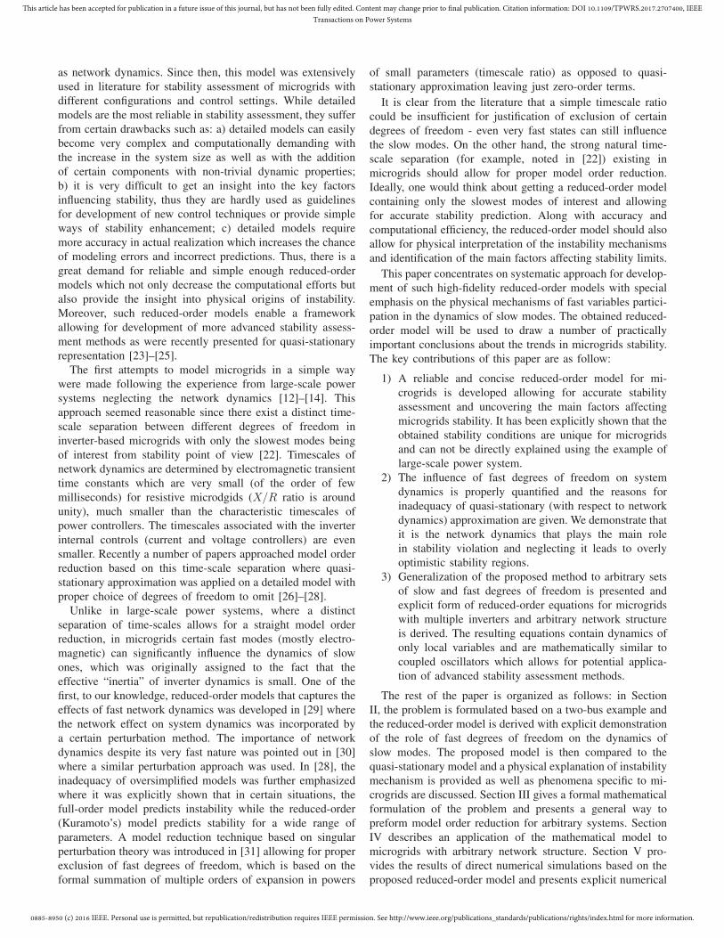
Fig. 1. The two-bus system under study. (a) Network configuration. (b) Two-loop controller. (c) Droop controller.
comparisons for different models under investigation. Finally,
conclusions are drawn in Section VI.
II. TWO-BUS MODEL
In this section, the microgrid stability problem that moti-
vates this study is illustrated using a simple two-bus system
shown in Fig. 1(a). We follow the standard two-loop control
system comprised of the inner current loop and outer voltage
loop with feed-forward compensations [22], as shown in Fig.
1(b). In general, the inner loop is designed to be much
faster than the outer one, allowing independent tuning of
the inner and outer control gains. While preventing over-
current references fed to the current controller, the overall
synthesized control achieves regulation of the filter capacitor
voltage based on the given voltage reference, V ∗
cd = U ,
V ∗
cq = 0 so that the LC filter can also be considered as a
part of this control scheme (since the tuning of both inner
and outer loops takes into account LC filter parameters).
Meanwhile, the integral of the frequency reference is used for
generating the pulsewidth-modulated (PWM) signal. Finally,
the frequency/voltage references are supplied by the droop
control as shown in Fig. 1(c).
Therefore, the following setting based on per-unit represen-
tation will be utilized in this section. A single inverter unit with
nominal power Sn in p.u. is connected to an infinite bus (fixed
voltage Us and frequency ω0) by a coupling impedance with
resistance Rc and inductance Lc and a line with resistance Rl
and inductance Ll. The inverter operates in a droop-controlled
mode 1(c), such that the equilibrium frequency is related to
the output real power while the inverter terminal voltage is
related to the reactive power according to the relations [22]:
ω = ωset −kpω0
Sn
P, U = Uset −kqSn
Q (1)
where Sn = Sinv/Sb denotes the inverter rating in respect
to the base power Sb, while ωset and Uset are the set points
of frequency and voltage controllers, respectively. It should
be noticed that we consider both ω and ω0 to be measured in
rad/s. The variables P and Q in (1) are the active and reactive
power filtered by means of passing the measured instantaneous
values (denoted as Pm and Qm) through a low-pass filter:
P =1
1 + τsPm, Q =
1
1 + τsQm (2)
where τ = ω−1c is the power controller filter time (or
the inverse of the filter cut-off frequency). The values of kpand kq are the per-unit frequency and voltage droop gains,
respectively. It should be noted that the droop gains kp and
kq are normalized to the individual inverter rating Sn (which
might be different for different inverters in the system) thus
representing a natural relative gain of each inverter. Typically,
the values of kp and kq are set within 0.5%− 3% [22].
For small-signal stability analysis of an AC system operat-
ing at equilibrium with a certain frequency ω0, it is convenient
to employ the following dynamic representation:
v(t) = Re[V (t)ejω0t]; i(t) = Re[I(t)ejω0t], (3)
where the complex amplitudes V (t) and I(t) can be ar-
bitrary (not necessarily slowly varying) functions of time. In
the case of grid-connected inverter, the equilibrium frequency
ω0 coincides with the grid frequency. The index 0 is used
throughout the paper to denote the equilibrium values of
corresponding variables. It should be noted that equations
(3) represent a mathematical change of functions and do not
introduce any approximation to dynamic equations - i.e., no
restrictions are imposed on how fast the phasors V (t) and I(t)can change. Similar representation is used in [29] and [30].
The rest of this section is organized as follows. First, an
initial model for a droop-controlled inverter that includes
both fast and slow variables is presented. Then, a simple
model order reduction technique based on the quasi-stationary
approximation is illustrated. Following we introduce a proper
model order reduction procedure explicitly demonstrating the
failure of the quasi-stationary model and uncovering the
physical mechanisms of fast degrees of freedom participation
in dynamics of slow modes. Then, an explicit comparison
with large-scale power systems is carried out to show why
the approaches used for the latter fail to properly describe
microgrids.
A. Electromagnetic 5th-Order Model
In our initial model, the inverter with its LC filter is
considered as an effective voltage source governed by the
slower droop control. Following this model, U∠θ is used
to represent the inverter effective terminal voltage and phase
angle after the LC filters. This allows us to effectively describe
the system using only inverter terminal states (angle, frequency
0885-8950 (c) 2016 IEEE. Personal use is permitted, but republication/redistribution requires IEEE permission. See http://www.ieee.org/publications_standards/publications/rights/index.html for more information.
This article has been accepted for publication in a future issue of this journal, but has not been fully edited. Content may change prior to final publication. Citation information: DOI 10.1109/TPWRS.2017.2707400, IEEETransactions on Power Systems
0 0.1 0.2 0.3 0.4 0.5 0.6 0.7 0.8 0.9 1
Time (s)
312.8
313
313.2
313.4
313.6
313.8F
req
ue
ncy (
rad
/s)
Detailed Model
Electromagnetic Model (EM)
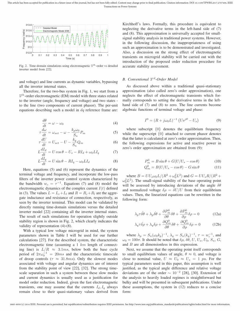
Fig. 2. Time-domain simulations using electromagnetic 5th-order vs detailedinverter model from [22].
and voltage) and line currents as dynamic variables, bypassing
all the inverter internal states.
Therefore, for the two-bus system in Fig. 1, we start from a
5th-order electromagnetic (EM) model with three states related
to the inverter (angle, frequency and voltage) and two states -
to the line (two components of current phasor). The per-unit
equations describing such a model in dq reference frame are:
dθ
dt= ω − ω0 (4)
τdω
dt= ωset − ω −
kpω0
Sn
Pm (5)
τdU
dt= Uset − U −
kqSn
Qm (6)
LdIddt
= U cos θ − Us −RId + ω0LIq (7)
LdIqdt
= U sin θ −RIq − ω0LId (8)
Here, equations (5) and (6) represent the dynamics of the
terminal voltage and frequency, and incorporate the low-pass
filters of the inverter power control system characterized by
the bandwidth wc = τ−1. Equations (7) and (8) model the
electromagnetic dynamics of the complex current I(t) defined
in (3). The values L = Lc+Ll and R = Rc+Rl are the aggre-
gate inductance and resistance of connection, respectively, as
seen by the inverter terminal. This model can be validated by
directly running time-domain simulations versus the detailed
inverter model [22] containing all the inverter internal states.
The result of such simulations for operation slightly outside
stability region is shown in Fig. 2, which clearly indicates the
validity of representation (4)-(8).
With a typical low voltage microgrid in mind, the system
parameters shown in Table I will be used for our further
calculations [27]. For the described system, the characteristic
electromagnetic time (assuming a 1 km length of connect-
ing line) is L/R ≈ 3.1ms, below both the base cycle
period of 2πω−10 = 20ms and the characteristic timescale
of droop controls (τ ≈ 31.8ms). Only the slowest modes
associated with voltage and angular dynamics are of interest
from the stability point of view [22], [32]. The strong time-
scale separation in such a system between these slow modes
and current dynamics is usually used as a justification for
model order reduction. Indeed, given the fast electromagnetic
transients, one may assume that the currents Id, Iq always
remain close to their quasi-stationary values derived from
Kirchhoff’s laws. Formally, this procedure is equivalent to
neglecting the derivative terms in the left-hand side of (7)
and (8). This approximation is universally accepted for small-
signal stability analysis in traditional power systems. However,
in the following discussion, the inappropriateness of using
such an approximation is to be demonstrated and investigated.
Also, a discussion on the strong effect of electromagnetic
transients on microgrid stability will be carried out with the
introduction of the proposed order reduction procedure for
accurate stability assessment.
B. Conventional 3rd-Order Model
As discussed above within a traditional quasi-stationary
approximation (also called zero’s order approximation), one
neglects the effect of electromagnetic transients which for-
mally corresponds to setting the derivative terms in the left-
hand side of (7) and (8) to zero. The line currents become
algebraic functions of terminal voltage and phase:
I0 = (R+ jω0L)−1
(
Uejθ − Us
)
(9)
where subscript 0 denotes the equilibrium frequency
while the superscript 0 attached to current phasor denotes
that the latter is calculated at zero’s order approximation. Then,
the following expressions for active and reactive power in
zero’s order approximation are obtained from (9):
P 0m = B sin θ +G(U/Us − cos θ) (10)
Q0m = B(U/Us − cos θ)−G sin θ (11)
where B = UUsω0L/(R2+ω2
0L2) and G = UUsR/(R2+
ω20L
2). The small-signal stability of the base operating point
will be assessed by introducing deviations of the angle δθand normalized voltage δρ = δU/U from their equilibrium
values. Then, the linearized equations can be rewritten in the
following form:
λpτ δθ + λpδθ +∂P 0
m
∂θδθ +
∂P 0m
∂ρδρ = 0 (12a)
λqτ δρ+ λqδρ+∂Q0
m
∂θδθ +
∂Q0m
∂ρδρ = 0 (12b)
where λp = Sn(ω0kp)−1, λq = Sn(kq)
−1, τ = w−1c , and
ω0 = 100π. It should be noted that δρ, δθ, U , Us, U0, Sn, G,
and B are all dimensionless in this expression.
Next, we assume that the operating point itself corresponds
to small equilibrium values of angle, θ ≈ 0, and voltage is
close to nominal value, U ≈ U0 ≈ Us = 1 pu. For the
typical parameters used in this paper, this assumption is well
justified, as the typical angle difference and relative voltage
deviations are of the order ∼ 10−2 [28], [30]. Extension of
the analysis to heavily loaded regimes is straightforward but
bulky and will be presented in subsequent publications. Under
these assumptions, the system in (12) reduces to a concise
form:

0885-8950 (c) 2016 IEEE. Personal use is permitted, but republication/redistribution requires IEEE permission. See http://www.ieee.org/publications_standards/publications/rights/index.html for more information.
This article has been accepted for publication in a future issue of this journal, but has not been fully edited. Content may change prior to final publication. Citation information: DOI 10.1109/TPWRS.2017.2707400, IEEETransactions on Power Systems
λpτ δθ + λpδθ +Bδθ +Gδρ = 0 (13a)
λqτ δρ+ (λq +B)δρ−Gδθ = 0 (13b)
The form of equations in (13) indicate that in the absence of
conductance, the dynamics of the angle and voltage deviations
become uncoupled and the system is always stable. Active
resistance introduces an effective positive feedback to the
system and may lead to the loss of stability. The detrimental
effect of the conductance on stability can be illustrated using
the following informal argument based on the multi-time-
scale expansion approach utilized in this work. Equation (13b)
implies that the voltage deviation follows the deviation of the
angle with some delay:
δρ(t) =G
λqτ
∫
∞
0
exp
[
−(λq +B)T
λqτ
]
δθ(t− T )dT, (14)
When dynamics of δθ is slow enough, the effect of delay
can be approximated as
δρ(t) ≈G
λq +Bδθ(t)−
λqτG
(λq +B)2δθ(t) (15)
This expansion can be obtained by applying a first-order
Taylor expansion to δθ(t−T ) in (14) and neglecting the con-
tribution of higher-order derivatives of δθ. Plugging expression
(15) back in (13a), the following approximation is obtained:
λpτ δθ +
[
λp −λqτG
2
(λq +B)2
]
δθ +
(
B +G2
λq +B
)
δθ = 0
(16)
The above approximation illustrates the effect of delay on
the system stability. For high conductance values, the effective
damping coefficient in front of δθ can become negative which
results into instability. This can happen for any arbitrary ratio
of timescales of the system modes, since the characteristic
timescale is not the only relevant parameter but rather it’s the
product with the corresponding gain. Assuming Sn = 1, the
system would remain stable whenever kp satisfies
kp <(1 + kqB)2
ω0kqτG(17)
This argument is not entirely rigorous since dynamics of δθis not necessarily slower than dynamics of δρ, although the
resulting condition on kp is reasonably accurate and highlights
the importance of delays. However, a similar procedure can
be applied to account for delays caused by the line inductance
which will be shown to be important for microgrids. In the
case of electromagnetic delays in lines the application of multi-
time-scale expansion is well justified since the electromagnetic
delay time is much smaller than the typical time-scale of
voltage and angle dynamics.
C. High-Fidelity 3rd-Order Model
As discussed above, the conventional (quasistationery) 3rd-
order model becomes inappropriate for microgrids because
electromagnetic transients start to play a critical role in the
onset of instability despite their short timescale (the inap-
propriateness of such a model was explicitely discussed in
[30] and [28]). Mathematically, these electromagnetic tran-
sients manifest themselves in the derivative terms of the left
hand side of (7) and (8) which cannot be fully neglected.
Nevertheless, it is possible to account for these transients by
deriving an effective 3rd-order model which will allow for
accurate stability assessment. We will refer to this model as
“high-fidelity model”. In Laplace domain, (7) and (8) can be
explicitly solved for Id and Iq via a first-order transfer function
I =Uejθ − Us
R+ jω0L+ sL=
I0
1 + sL/(R+ jω0L). (18)
Whenever the goal is to derive an equivalent reduced-order
model capturing the dynamics of slow modes, it is reasonable
to assume that |sL/(R + jω0L)| ≪ 1 holds for modes that
evolve on the time-scales slower than the electromagnetic time
L/R. In this case, one can perform Taylor series expansion
on (18) to get
I ≈ I0 −Ls
R+ jω0LI0. (19)
Returning back to the time domain, (19) can be rewritten
as
I ≈ I0 −L
R+ jω0L
dI0
dt(20)
Then, the approximate values of Pm and Qm are obtained
as follows (detailed derivation is provided in Appendix A):
Pm ≈ P 0m −G′ρ−B′θ (21)
Qm ≈ Q0m −B′ρ+G′θ, (22)
where G′ and B′ are given by
G′ =L(R2 − ω2
0L2)
(R2 + ω20L
2)2; B′ =
2ω0RL2
(R2 + ω20L
2)2. (23)
Hence, the real and reactive powers now depend not only
on the voltage magnitude and angle values, but also on their
rates of change. In general, the terms with derivatives in (21)
are small compared to the quasi-stationary contribution from
P 0m and Q0
m, which justifies the expansion; however, these
terms will contribute to the corresponding derivative terms in
the dynamic equations. The equations for angular and voltage
dynamics, instead of (13) now become:
λpτ δθ + (λp −B′) δθ +Bδθ +Gδρ−G′δρ = 0 (24a)
(λqτ −B′) δρ+ (λq +B)δρ−Gδθ +G′δθ = 0 (24b)
These equations can be analyzed in a similar way to
obtain a generalized version of (17). However, some important
straightforward qualitative conclusions can be made from the
basic structure of (24). The natural negative feedback terms
for δθ and δρ can change sign when the corresponding droop
coefficients are increased (meaning the decrease in λp and/or

0885-8950 (c) 2016 IEEE. Personal use is permitted, but republication/redistribution requires IEEE permission. See http://www.ieee.org/publications_standards/publications/rights/index.html for more information.
This article has been accepted for publication in a future issue of this journal, but has not been fully edited. Content may change prior to final publication. Citation information: DOI 10.1109/TPWRS.2017.2707400, IEEETransactions on Power Systems
λq) - the effect is exclusively due to the network dynamics and
was not present in the conventional 3rd-order model. Thus, a
simple set of stability conditions can be obtained by requiring
these terms in front of the first derivatives to be positive, i.e.,
(λp −B′) > 0 and (λqτ −B′) > 0 which upon substitution
of λp, λq and B′ turns into:
kp < Sn
(R2 +X2)2
2RX2; kq < τω0Sn
(R2 +X2)2
2RX2, (25)
where X = ω0L. It is important to emphasize that the small
timescale of the electromagnetic phenomena L/R cannot be
used as a reliable indicator of the insignificance of the network
dynamics. Specifically, even if the second term in (20) is small
compared to the first (which is actually the case and is the
justification for expansion), this term contributes to a different
order of derivative in the dynamic equation (the derivative
terms in (24)), so that the true conditions on the insignificance
of network dynamics are B′ ≪ λp and B′ ≪ τλq with
the former being usually stronger. To avoid confusion, we
note that relations (25) do not represent the exact stability
criteria but rather give a general estimation of the small-
signal stability boundary in terms of frequency and voltage
droop coefficients and are very good for demonstrating the
key factors affecting stability as well as validity of the model.
The general observations from (25) are:
1) Decrease in the line reactances and resistances (i.e.,
improving the connection to the grid) has a deteriorating
effect on stability.
2) Decreasing the inverter rating (i.e., connecting smaller
inverter with the same relative settings and same cou-
pling impedance) reduces stability region.
3) Increasing the inverter control filtering time affects the
small-signal stability boundary mainly with respect to
the voltage droop gain.
These general stability properties have no analogy on the
level of large-scale power systems. In fact, the first two
are exactly the opposite of what has been well known for
transmission grids where improving the network connections
always has a positive effect on stability [33]. Below we give
a more detailed discussion of each of these properties verified
by the corresponding direct numerical simulations based on
the initial EM model.
A comparison of three different models (the 5th-order EM
model presented in (4)–(8), the conventional 3rd-order model
and the proposed high-fidelity 3rd-order model) is presented
in Fig. 3 with the predicted stable region being to the left
of the corresponding curve. The droop coefficients relative to
inverter rating are used as relevant parameters for stability
regions representation. It is obvious that the electromagnetic
transients play important role in stability violation and that
the conventional 3rd-order model is highly inappropriate for
stability assessment since it predicts a substantially larger sta-
bility region than the other two models (as was pointed in [28],
this simple oscillator-type model predicts stable operation for
almost any realistic microgrid configuration). It is important
to note that according to (24a) and (24b), the electromagnetic
modes start to be relatively unimportant if one considers only
EM model
Proposed 3rd order
Simple 3rd order
0.00 0.01 0.02 0.03 0.04 0.05
0.00
0.02
0.04
0.06
0.08
0.10
0.12
0.14
Frequency droop coefficient kp
Voltagedroopcoefficientkq
Fig. 3. Comparison of stability regions predicted by three different models(EM model refers to the electromagnetic 5th-order model).
sufficiently small values of droop coefficients corresponding to
λp ≫ B′ and λq ≫ B′ thus being far away from the stability
boundary. Any dynamic simulations in this region using either
of the models (quasi-stationary 3rd-order, high-fidelity 3rd-
order or 5th-order EM) will give very similar results. This is an
important observation, since it states that dynamic simulations
for a certain microgrid setting can be misleading in terms
of the model verification - one has to specifically look for
stability boundary predicted by the model in order to test its
validity. The numerical simulations confirming this statement
are provided in Section V.
D. Effect of line impedance
The numerical simulation using a 10 kVA inverter connected
to a grid through a line with parameters given in Table
I produces a stability boundary of kp ∼ 0.5 − 2% and
kq ∼ 2 − 25% depending on the connecting line length and
filter time constant. The result is specific to microgrids and
has no analogy to large-scale transmission grids, and can be
understood in the following way. Let us use a term “line
rating” to refer to a quantity Sl ∼ V 2/Zl which represents an
order of magnitude of power that can be transmitted over a line
until the formal violation of angular and/or voltage stability.
Let us assume that the line resistance and reactance are of
the same order (which is true for low-voltage grids under
consideration). Then, according to (25), the maximum value
of relative frequency droop coefficient is simply the ratio of
inverter rating to line rating. For the parameters under consid-
eration, the line rating is of the order of several hundreds of
kVA (for a 1km line with parameters from Table I, the rating
is around 750kV A) which is two orders of magnitude higher
than the typical inverter rating. Contrary to large transmission
systems, where power flows are mostly limited by voltage
drop and angular stability, the main limitation in microgrids
is the heating overcurrent limit of conductors. Consequently,
microgrids typically operate in a region of very small values
of inverter angles θ (or, more precisely, angle differences), this
fact was also noted in [30]. For large transmission systems,
generator ratings are usually of the same order as line ratings
(mainly due to machine internal inductances) and, hence, the
formal stability limit for machine is around kp ∼ 100% which
is never used in practice for other reasons.

0885-8950 (c) 2016 IEEE. Personal use is permitted, but republication/redistribution requires IEEE permission. See http://www.ieee.org/publications_standards/publications/rights/index.html for more information.
This article has been accepted for publication in a future issue of this journal, but has not been fully edited. Content may change prior to final publication. Citation information: DOI 10.1109/TPWRS.2017.2707400, IEEETransactions on Power Systems
l=0 km
l=0.2 km
l=0.4 km
0.000 0.005 0.010 0.015 0.020 0.025 0.030
0.00
0.02
0.04
0.06
0.08
0.10
0.12
0.14
Frequency droop coefficient kp
Voltagedroopcoefficientkq
Fig. 4. Stability regions for different lengths of connection line.
For the microgrid network under consideration, on the
contrary, a narrow stability boundary is shown - around
kp ∼ 1% which is roughly the ratio of inverter rating to
“line rating”. In fact, by assuming that the X/R ratio of
the connection is fixed (although it is slightly distorted by
the presence of coupling inductance which can have an X/Rdifferent from that of the network), then the term B′ is simply
inversely proportional to connection length, so is the maximum
frequency droop coefficient. It is, therefore, the absence of
large impedance which makes the inverter-based microgrids
completely different from large-scale power systems and syn-
chronous machine-based grids in terms of stability. A syn-
chronous machine connected to a low-voltage grid also does
not exhibit instabilities at such low values of frequency droop,
despite the fact that such machines can formally be described
by equations similar to (5)-(8), since machines normally have
large internal reactance X ′ ∼ 0.2− 0.5 which makes the term
B′ smaller. From this point of view, one can also give a rather
simple explanation why the electromagnetic transients are not
important for large-scale power systems and even for small-
scale synchronous machines (despite the larger timescale of
these transients compared to inverter-based microgrids due
to more inductive impedances of machines). Specifically, the
effect of electromagnetic transients is negligible if the B′ term
in (24a) and (24b) is much smaller than λp. The former has
an order of magnitude similar to the inverse impedance in
p.u. which for large-scale power grids is around unity, while
the latter is the inverse frequency droop - at least one order
of magnitude higher. Moreover, these effects are not directly
related to the generator time constant or, in the case of inverter,
the filter time constant τ (while the constant τ does affect
stability region (Fig. 6 ), it has no direct connection with
the validity of quasi-stationery approximation), which is often
mentioned as the main reason for the importance of network
dynamics for microgrids. It is rather the small per-unit values
of network characteristic impedances that makes it necessary
to consider electromagnetic transients.
The influence of different connecting line lengths on stabil-
ity is illustrated in Fig. 4 with the blue curve corresponding
to direct inverter connection and the effective line impedance
is only due to the internal coupling impedance. As noted in
Fig. 4, the increase in the connecting line impedance tends
to increase the overall stability region especially in terms of
voltage droop coefficient. While there is no strict monotonic
dependence of the maximum frequency droop coefficient on
the connecting line lengths, there seems to exist a robust
stability region corresponding to the lower left corner of Fig.
4 which is due to the minimum coupling impedance always
being present in the system. It is important to note that the
stability region can be expanded either by using lines with
greater impedance (especially with large reactance) or by
adding substantial amount of virtual impedance. In this case,
equations (24a) and (24b) as well as the relations in (25) can
give a key on the proper sizing of this virtual impedance for
a given set of target droop coefficients.
Let us also give a rather simple physical interpretation to the
instability mechanism in terms of time delays in network cur-
rent. One can think about the exact current i(t) being retarded
with respect to quasi-stationary value i0 by the characteristic
electromagnetic time L/R which decreases as R increases,
such that one might expect the quasi-stationary approximation
(conventional 3rd-order model) to work better with decreasing
X/R ratio. However, it is not the delay itself, but rather the
product of delay and gain that determines the overall effect
on stability. While the delay time is inversely proportional to
R, the corresponding gain, which is determined by the 1/B′
term in (24a) and (24b), is proportional to R2 so that the quasi-
stationary approximation becomes less applicable for resistive
lines despite the decrease in electromagnetic delay times.
E. Inverter Rating and Power Filter Time Constants
According to (25), the inverter rating has major influence
on the stability boundary in terms of the relative voltage and
frequency droop coefficients. In fact, one can refer directly to
(24a) and (24b) to infer the role of inverter rating. Stability
regions in the space of relative droop coefficients for inverters
of ratings 5, 10 and 20 kVA, respectively, are illustrated in Fig.
5. The stability criteria for small inverters are becoming stricter
with the acceptable values of relative frequency droop kpbecoming less than 0.5%. An important practical conclusion
from this observation is that connecting few smaller inverters
instead of a single larger one while keeping the same relative
settings for droop controls can lead the system to instability.
To avoid any confusion, it should be pointed out that if one sets
the absolute droop coefficients in (rad/s)/W and V/V AR,
respectively, the stability is not affected by the inverter rating.
It is however reasonable to consider the droop settings in
relative units, similar to the way it is done in large-scale power
systems.
Equation (25) also allows for drawing some general conclu-
sions about the influence of the power filters cut-off frequency
on stability regions. The filtering time constant plays a role
of “inertia” and is considered to be one of the major factors
influencing stability. Equation (25) suggests that the filtering
time constant has the most affect on the small-signal stability
region with respect to the voltage droop coefficient value,
which is confirmed by direct numerical simulations given in
Fig. 6. Increasing the inverter filter time constant significantly
broadens the stability region; however, extension to the larger

0885-8950 (c) 2016 IEEE. Personal use is permitted, but republication/redistribution requires IEEE permission. See http://www.ieee.org/publications_standards/publications/rights/index.html for more information.
This article has been accepted for publication in a future issue of this journal, but has not been fully edited. Content may change prior to final publication. Citation information: DOI 10.1109/TPWRS.2017.2707400, IEEETransactions on Power Systems
Sn=0.5 pu
Sn=1 pu
Sn=2 pu
0.000 0.005 0.010 0.015 0.020 0.025 0.030 0.035
0.00
0.02
0.04
0.06
0.08
0.10
Frequency droop coefficient kp
Voltagedroopcoefficientkq
Fig. 5. Stability regions for different inverter rating values, 1 pu =10 kVA.
ωc=31.41 rads/s
ωc=20.94 rads/s
ωc=15.71 rads/s
0.000 0.005 0.010 0.015 0.020 0.025 0.030 0.035
0.00
0.02
0.04
0.06
0.08
0.10
Frequency droop coefficient kp
Voltagedroopcoefficientkq
Fig. 6. Stability regions for different power filter cut-off frequencies.
0.6 0.8 1.0 1.2 1.4 1.6 1.8 2.0
0.12
0.13
0.14
0.15
0.16
0.17
0.18
X/R Ratio
B'
Fig. 7. Variation of B′ with respect to X/R ratio.
values of frequency droop is only possible if the voltage droop
is varied correspondingly (as seen in Fig.6).
F. Virtual Impedance Methods
It has been shown previously that the stability region of the
droop-controlled inverter system is constrained mainly due to
the presence of B′ term in (24a) and (24b). This, so-called,
transient susceptance B′ becomes larger as a result of stronger
coupling between the inverter and the grid. In [17], it has
been indicated that installation of additional coupling inductors
is recommended for enhancing the stability, however, such a
bulky inductor is not always desirable. Thus, several research
works have proposed the concept of virtual impedances, virtual
inductances or virtual synchronous generators [16], [17], [34],
[35].
As mentioned previously, we follow a standard two-loop
control concept consisting of inner current and outer voltage
X/R=0.5
X/R=1.0
X/R=2.0
0.000 0.005 0.010 0.015 0.020
0.00
0.02
0.04
0.06
0.08
0.10
Frequency droop coefficient kp
Voltagedroopcoefficientkq
Fig. 8. Stability regions for different X/R ratios.
loops. In general, the response of voltage regulation is fast
enough to allow synthesizing different dynamic behaviors.
Therefore, to mimic the virtual impedance, additional terms
that react to the output currents are added for emulating the
inductive dynamics. That is, the modified reference voltages
in Fig. 1 are given by the following forms:
V ∗
cd =U +XmIq −sωfLm
s+ ωf
Id (26a)
V ∗
cq =0−XmId −sωfLm
s+ ωf
Id (26b)
where Xm = ω0Lm denotes the virtual reactance, ωf is the
cut-off frequency of the high-pass filter, V ∗
cd,cq are the modified
reference voltages for the two-loop control scheme, and Id,qare the output currents in dq axis. One can note that the above
mentioned control scheme may have different equivalent forms
that result in similar dynamic behavior, and here we follow
a configuration similar to one proposed in [34]. Details of
particular implementation are beyond the scope of this paper.
With the deployment of virtual impedances/inductances,
expansion of the stability region can be explained by con-
sidering the change of corresponding B′ = 2RX2/(ω0Z4)
value, whose variation with X/R ratio is shown in Fig. 7,
where X = ω0(Lm + Ll + Lc) and R = Rl + Rc. Thus,
equations (24a) and (24b) give a guideline for proper sizing of
the virtual impedance if achieving stability for certain droop
coefficients is targeted. It can be seen that the value of B′
peaks when X/R = 1, implying that bidirectional perturbation
of X/R away from unity allows expansion in stability range
of kp assuming that kq is sufficiently small. That is, when the
interaction between droop and voltage modes is weak (low kq),
a negative damping coefficient of θ in (24a) leads to instability.
As shown in Fig. 8, however, decreasing X/R may further lead
to shrinking the stable kp range with a higher kq . In general,
it is more beneficial to properly select the virtual impedance
to ensure X/R > 1 for further expansion of stability region.
III. GENERALIZED MULTI-TIMESCALE APPROACH
In this section, a formulation of a general method for
stability analysis of multiple timescale systems is presented.
The method represents a first-order of the, so-called, singular

0885-8950 (c) 2016 IEEE. Personal use is permitted, but republication/redistribution requires IEEE permission. See http://www.ieee.org/publications_standards/publications/rights/index.html for more information.
This article has been accepted for publication in a future issue of this journal, but has not been fully edited. Content may change prior to final publication. Citation information: DOI 10.1109/TPWRS.2017.2707400, IEEETransactions on Power Systems
perturbation theory as opposed to zero-order, which corre-
sponds to neglecting the dynamics of fast variables altogether.
Employing this method allows for proper inclusion of possible
effect fast variables have on slow modes. The presence of
strong timescale separation in microgrids manifests itself in
the appearance of several clusters of modes on the plane of
system eigenvalues with only one cluster, corresponding to
the slowest modes, associated with power controllers, is of
interest from the point of view of small-signal stability [22],
[32]. Let us start from the general description of a system with
a set of first-order differential equations linearized around an
equilibrium point:
δx = Aδx (27)
where x is a set of system variables and A is the corresponding
Jacobian matrix. It is desirable to aim at such a simplification
of a system representation, that only the relevant modes are
considered in the form of dynamic equations and all the
rest are properly eliminated. The timescale separation was
presented in [27] where the authors introduced a two time-
scale model of a system and completely excluded the dynamics
of “fast” variables by using their quasi-stationary values and
considered three different ways of separating the initial set into
“fast” and “slow” degrees of freedom. In the present paper,
a more systematic procedure of timescale separation will be
presented along with a procedure for proper exclusion of fast
degrees of freedom while accounting for their effect in the
reduced-order system.The separation of the system in (27) into
two subsystems corresponding to slow and fast variables gives:
δxs = Assδxs +Asfδxf (28)
Γδxf = Afsδxs +Affδxf (29)
where the subscripts s and f correspond to slow and fast
degrees of freedom, respectively; Γ is a set of parameters
designating fast degrees of freedom. A procedure employed
in [27] neglects the left-hand side of (29), thus reducing the
system in (28) to the following (see Appendix B for details):
δxs = (Ass −AsfA−1ff Afs)δxs (30)
The stability of such a system is certified by demanding all
the eigenvalues of the new state matrix (Ass − AsfA−1ff Afs)
to have negative real parts.
Expression (30) can be treated as a zero’s order approxi-
mation of the perturbation approach. It is formally obtained
by stating a linear relation between δxf and δxs which is
found from (29) by neglecting its left-hand side (details are
provided in Appendix B). Let us now consider the next order
by stating that the first derivative of δxf is non-zero (i.e.,˙δxf 6= 0), but the second derivative is negligible. Inserting
such a dependence in (29) and separating different orders of
magnitude, one finds:
δxf = −A−1ff Afsδxs −A−1
ff ΓA−1ff Afsδxs (31)
Inserting this into (28), the following is obtained:
(1+AsfA−1ff ΓA
−1ff Afs)δxs = (Ass−AsfA
−1ff Afs)δxs (32)
which is a generalization of (30) and 1 in the left-hand side
of (32) represents a unity matrix. The described procedure is
rather general and incorporates the cases when some of the
fast degrees of freedom are “instantaneous” which correspond
to respective elements of Γ being zero such that algebraic
constraints can also be treated. The convenience of the rep-
resentation used lies in the fact that one can operate with a
general set of fast degrees of freedom without the need to first
separate the linearly independent ones or solve for individual
variables derivatives.
The general expression (32) can be used in order to explain
why the fast degrees of freedom can play an important role in
system stability and why using quasi-stationary approximation
can be unjustified. The stability of such a system is certified
only if the full state matrix (Ass − AsfA−1ff Afs)
−1(Ass −
AsfA−1ff Afs) satisfies the Routh-Hurwitz criterion. It is not
uncommon that the quasi-stationery state matrix (Ass −AsfA
−1ff Afs) has all the real parts of its eigenvalues negative,
thus certifying the stability of the quasi-stationary system (30)
while the full state matrix has positive real parts of one or more
of its eigenvalues making the whole system unstable. This is
exactly the case with the stability of a droop-controlled inverter
connected to an external grid which was considered in details
in the previous section.
The influence of fast degrees of freedom is described by
the term AsfA−1ff ΓA
−1ff Afs which is added to a unity matrix.
While the timescale parameters Γ can be arbitrarily small,
it is not the components of matrix Γ itself that should be
compared to unity, but rather the components of the matrix
AsfA−1ff ΓA
−1ff Afs which are not necessarily small. This il-
lustrates why a simple observation of time-scales (looking at
components of Γ matrix) of the initial problem can not give
a reliable conclusion about the possibility to omit a certain
degree of freedom from dynamic equations. One should look
at the components of the matrix AsfA−1ff ΓA
−1ff Afs in order
to judge whether the role of fast state is significant or not.
IV. NETWORK GENERALIZATION
A general approach derived in the previous section can be
used to derive a reduced-order system of dynamic equations
for microgrids with multiple inverters and loads. Formally, the
method can be applied to microgrids with arbitrary structure
including those containing loads with nontrivial dynamics - at
the first step one needs to separate the “slow” and “fast” states
and then follow the described procedure to arrive to equa-
tions (32). Here, an application of the method to microgrids
containing multiple droop-controlled inverters and constant
impedance loads will be presented. It is important to note that
this procedure can be also directly applied to networks with
constant power loads (CPL) and current-controlled inverters,
which should be simply treated as constant power sources
(CPS). Although the power consumed by CPL or dispatched
by CPS can change on larger timescales, for small-signal
stability studies it is sufficient to treat them as constant power

0885-8950 (c) 2016 IEEE. Personal use is permitted, but republication/redistribution requires IEEE permission. See http://www.ieee.org/publications_standards/publications/rights/index.html for more information.
This article has been accepted for publication in a future issue of this journal, but has not been fully edited. Content may change prior to final publication. Citation information: DOI 10.1109/TPWRS.2017.2707400, IEEETransactions on Power Systems
components by taking a snapshot of operating conditions for
a given instant. The influence of power electronics controlled
CPL on the stability of inverter-based microgrids has been
extensively studied in [36] with the conclusion that there is
limited effect from the load dynamics on the power controllers
of inverters. Therefore, for the purpose of small-signal stability
studies of a microgrid containing droop-controlled inverters
along with non-dispatchable DGs and constant power loads,
the two latter components can be effectively substituted by
their linearized equivalent impedances. In the following, we
use the term “inverter” only in reference to droop-controlled
ones, all the remaining components of a microgrid (like
current-controlled inverters) are referred to as loads or sources
and treated as described above.
Generalization of the proposed model presented in Section
II to networks is done directly by constructing a system of dy-
namic equations similar to (24) for every inverter node. First,
a network admittance matrix Y(s) (in Laplace representation)
should be constructed using the full network impedance matrix
where all the line and effective load impedances Zij(s) are
written in Laplace domain (i.e., Zij = Rij + jω0Lij + sLij).
Matrix Y(s) links inverter voltages to inverter currents:
I(s) = Y(s)V(s) (33)
where I(s) and V(s) are the Laplace transforms of the
complex vectors of inverter currents and voltages, respectively.
The equivalent network contains inverter buses that are inter-
connected through lines in addition to shunt elements attached
to inverter buses to represent loads. It is convenient to separate
the total admittance matrix into the “network” (denoted by
index N ) and the “load” (denoted by index L) parts:
Y(s) = YN (s) +YL(s) (34)
where the “load” admittance matrix YL(s) is diagonal.
Then, the next step is to expand the admittance matrix using
first-order Taylor expansion:
Y(s) ≈ Y0 +Y1s (35)
where
Y0 = Y(s)|s=0 (36)
Y1 =∂Y(s)
∂s|s=0 (37)
After substitution in (33) and switching back to time do-
main, a generalized version of (20) is obtained:
I(t) = [Y0N +Y0L]V(t) + [Y1N +Y1L] V(t) (38)
One can note that in general it is not appropriate to use the
quasi-stationary reduced admittance matrix (Y0) for network
dynamic simulation, since the proper network representation
should be calculated using the initial structure with full
impedances (including the Laplace parameter s).
Then, the relations (35) and (38) can be used to construct
the generalized dynamic equations of a system with intercon-
nected inverters and loads and, similarly to (24) we get:
τΛpϑ+ (Λp −B′)ϑ+Bϑ+ (G+ G)−G
′ ˙ = 0 (39a)
(τΛq −B′) ˙ + (Λq +B+ B)−Gϑ+G
′ϑ = 0 (39b)
where ϑ and are vectors of inverter angles and (relative)
voltages, respectively; and all the terms in bold are square
matrices with dimensions corresponding to the number of
inverters in the grid. Λp and Λq represent the diagonal
matrices with elements equal to the inverse of frequency and
voltage droop coefficients, respectively.
Matrices B, B, G and G can be expressed in terms of the
quasi-stationary network admittance matrix:
B = −U20 Im Y0N , G = U2
0 Re Y0N (40)
B = −2U20 Im Y0L , G = 2U2
0 Re Y0L (41)
It is important to note that both B and G are singular but
positive semi-definite matrices, while B and G are diagonal
and positive-definite matrices. Matrices B′ and G
′ represent
the effect of network and load dynamics, and can be expressed
in terms of Y1:
B′ = U2
0 Im Y1N +Y1L (42a)
G′ = −U2
0 Re Y1N +Y1L (42b)
Since B′ and G
′ are obtained from the admittance matrix
through linear operation, they preserve the general property:
diagonal element is equal to the negative sum of all elements
in a corresponding row plus the shunt admittance due to a
load attached to the corresponding bus. One can also note
that matrix B′ is positive definite, while matrix G
′ is sign
indefinite. Typically, the equivalent impedances of loads are
much larger than the impedances of the lines, so one would
expect their effect to be negligible (this is also confirmed in
[36] and [37]).
Equations (39) allow one to analyze the stability of a multi-
inverter system taking into account the network dynamics,
while still having an effective low-order form with simple
representation of droop coefficients. The main value of such
a representation is that the resulting equations contain only
local (i.e. related to a single inverter) dynamic states with
all the non-local variables being properly excluded. Such a
property of dynamic equations is crucial for development of
certain advanced methods for stability assessment [23]–[25],
however, as was explicitly pointed out in [28], a simplified rep-
resentation with network dynamics neglected does not allow
for proper assessment of microgrids stability. Therefore, an
important contribution of this work is that it introduces a new
model for microgrids stability study possessing the simplicity
of oscillator-type quasi-stationary reduced-order models but
at the same time properly accounting for important network
dynamics. Any existing techniques that are known for quasi-
stationary approximation can now be directly applied to this
model with the network dynamics effects automatically taken
into account.

0885-8950 (c) 2016 IEEE. Personal use is permitted, but republication/redistribution requires IEEE permission. See http://www.ieee.org/publications_standards/publications/rights/index.html for more information.
This article has been accepted for publication in a future issue of this journal, but has not been fully edited. Content may change prior to final publication. Citation information: DOI 10.1109/TPWRS.2017.2707400, IEEETransactions on Power Systems
Fig. 9. System configuration of inverter-based microgrid under study.
0 0.2 0.4 0.6 0.8 1 1.2 1.4
(a) Time (s)
313.15
313.2
313.25
313.3
Fre
quency (
rad/s
)
EM model
Proposed 3rd order
Simple 3rd order
0.2 0.4 0.6 0.8 1 1.2 1.4
(b) Time (s)
312.24
312.26
312.28
312.3
312.32
312.34
312.36
312.38
312.4
Fre
quency (
rad/s
)
EM model
Proposed 3rd order
Simple 3rd order
Fig. 10. Dynamic responses of different models with different droop gains.(a) kp = 0.45%. (b) kp = 0.75%.
V. NUMERICAL EVALUATION
A. Model Accuracy
In this section, simulation results comparing the different
models are presented. To verify the accuracy of the proposed
reduced-order model, a system with five inverters in the
cascade configuration shown in Fig. 9 is investigated, in which
the coupling inductors are included into the network in Y
representation. The system parameters of five inverter-based
microgrid are given in Table I in the Appendix. First, a time-
domain simulation was conducted to compare the dynamic
responses predicted by different models for different values of
droop coefficients, as shown in Fig. 10. It is shown that all
-40 -30 -20 -10 0 10
real
-100
-50
0
50
100
imag
EM model
Proposed 3rd order
Simple 3rd order
Fig. 11. Eigenvalue plots of different models (kp = 0.3%− 0.75%).
the models match very well when the operating droop gains
are far away from the instability boundary which is shown
in Fig. 10(a). The discrepancies between the models become
significant when the system reaches instability as shown in
Fig. 10(b), where erroneous prediction of stable operation can
be observed from the conventional simple 3rd-order model,
while the EM and the developed high-fidelity model give
correct prediction of the onset of instability. We would like
to emphasize that the performance of reduced-order model in
dynamic simulations for certain number of operating points
is not a sufficient indicator of the model quality - one needs
to look at the stability boundaries predicted by the model in
order to draw conclusions about its accuracy. Furthermore,
a comparison of eigenvalue movements by varying kp for
different models is given in Fig. 11. It can be seen that the
eigenvalues of the system calculated using the proposed 3rd-
order model are much closer to the EM model as compared
to the simple 3rd-order model, which is consistent with the
simplified two-bus results presented in Section II.
B. Simulation Efficiency
Another important feature of the proposed reduced-order
model is that it mitigates the computation burden on the time-
domain simulation. For the EM model, all the cable and load
dynamics are modelled as states. The total number of states
(ns) is approximately 9 times the number of inverters in
the cascade topology. In comparison, the proposed technique
requires only 3 states per inverter, which reduces the number of
states by two-thirds. This allows us to handle a network system
with a large number of inverters. To identity the efficiency of
the proposed model, the EM and proposed 3rd-order models
are tested via time-domain simulation with Matlab default
O.D.E. solvers. The inverters, coupling inductors, and the
lines/cables are assumed to be identical for simplicity. The
simulation time is set to be one second. The results are shown
in Table II for 5 and 25 inverter-based microgrids. These
results clearly demonstrate that the proposed model reduces
the number of states and improves the simulation efficiency
significantly.

0885-8950 (c) 2016 IEEE. Personal use is permitted, but republication/redistribution requires IEEE permission. See http://www.ieee.org/publications_standards/publications/rights/index.html for more information.
This article has been accepted for publication in a future issue of this journal, but has not been fully edited. Content may change prior to final publication. Citation information: DOI 10.1109/TPWRS.2017.2707400, IEEETransactions on Power Systems
VI. CONCLUSION
Contrary to large-scale power grids, network dynamics of
microgrids, despite it’s faster time-scales, can greatly influence
the behavior of slow degrees of freedom associated with
inverter power controllers. Particularly, the stability region
in terms of voltage and frequency droop coefficients is sig-
nificantly diminished compared to the one predicted by a
simple quasi-stationary model. In this paper, an insight to
the physical mechanism of instability is presented along with
a method for proper exclusion of fast network degrees of
freedom without compromising the accuracy of the model
while bringing major simplifications in terms of computational
complexity and model transparency. The influence is reflected
in the corresponding change of the coefficients of the resulting
3rd-order model compared to a purely quasi-stationary approx-
imation (neglecting the fast degrees of freedom altogether)
which leads to significant changes in the predicted regions
of stability. The proposed technique is used to illustrate the
microgrid specific effects, namely deterioration of stability
by reduction of network impedances and/or inverter ratings.
The proposed technique is then generalized to microgrid with
multiple inverters and arbitrary network structure where the
dynamic equations with only local state variables are derived.
Future studies will focus on the development of more advanced
stability assessment methods based on the proposed reduced-
order model. The method of Lyapunov functions may allow
for formulation of stability criteria dealing with each inverter’s
droop coefficients and connecting lines separately or with
pairs of interconnected inverters. Such criteria can be used
for assessment of stability during system reconfiguration or
multiple microgrid interconnection.
APPENDIX A
Here, we provide the detailed derivation of equation (24).
First, let us start from the general expression Pm + jQm =UejθI∗. The current phasor approximation is given by (20)
with I0 given by (9). By taking the time derivative, one
obtains:
I ≈ I0 −L
(R+ jω0L)2
[
Uejθ − jθUejθ]
(43)
Then, by taking the conjugate of (43) and multiplying by
the voltage phasor Uejθ, one can get:
Pm+jQm = P 0m+jQ0
m−L
(R− jω0L)2
[
UU + jθU2]
(44)
After separation of the real and imaginary part and setting
U ≈ Ub = 1pu in the second term in the right-hand side,
the expression from (21) is obtained (we also use θ = δθ,
U = ˙δU ).
APPENDIX B
Here, the detailed derivation of equation (32) is provided.
First, let us start from the initial equation for fast states
dynamics:
TABLE IPARAMETERS OF FIVE INVERTER-BASED MICROGRID
Parameter Description Value
Ub Base Peak Phase Voltage 381.58V
Sb Base Inverter Apparent Power 10 kVA
ω0 Nominal Frequency 2π×50 rad/s
Lc Coupling Inductance 0.35mH
Rc Coupling Resistance 30mΩ
wc Filter Constant 31.4 rad/s
mp Default P − ω Droop Gain 9.3× 10⁻⁵ rad/s/W
nq Default Q− V Droop Gain 1.3× 10⁻³ V/VAR
Ll Line Inductance 0.26mHkm−1
Rl Line Resistance 165mΩkm−1
lij Line Length [5, 4.1, 3, 6] km
Z1 Bus 1 Load 25 Ω
Z2 Bus 2 Load 20 Ω
Z3 Bus 3 Load 20 + 4.72i Ω
Z4 Bus 4 Load 40 + 12.58i Ω
Z5 Bus 5 Load 18.4 + 0.157i Ω
X/R Average X/R Ratio 0.6224
Γδxf = Afsδxs +Affδxf (45)
Then, we seek for δxf as a series:
δxf ≈ δx(0)f + δx
(1)f + δx
(2)f ... (46)
where superscripts in brackets designate the orders of per-
turbation expansion. For our purposes, we only need the zeros
and first order terms. Inserting them into (45) will give:
Γδx(0)f + Γδx
(1)f = Afsδxs +Affδx
(0)f +Affδx
(1)f (47)
Separating the zero and first order terms (in this respect,
the second term in the left-hand side has a second order and
should be omitted), one can find:
Afsδxs +Affδx(0)f = 0 (48)
Γδx(0)f = Affδx
(1)f (49)
Then, the following expressions are obtained:
δx(0)f = −A−1
ff Afsδxs (50)
δx(1)f = −A−1
ff ΓA−1ff Afs
˙δxs (51)
Inserting these expressions into the equations for slow
degrees of freedom in (28), one arrives to (32).
REFERENCES
[1] N. Hatziargyriou, H. Asano, R. Iravani, and C. Marnay, “Microgrids,”IEEE Power Energy Mag., vol. 5, no. 4, pp. 78–94, 2007.
[2] R. H. Lasseter, “Smart distribution: Coupled microgrids,” Proceedings
of the IEEE, vol. 99, no. 6, pp. 1074–1082, 2011.
[3] M. Smith and D. Ton, “Key connections: The us department of energy?s microgrid initiative,” IEEE Power and Energy magazine, vol. 11, no. 4,pp. 22–27, 2013.

0885-8950 (c) 2016 IEEE. Personal use is permitted, but republication/redistribution requires IEEE permission. See http://www.ieee.org/publications_standards/publications/rights/index.html for more information.
This article has been accepted for publication in a future issue of this journal, but has not been fully edited. Content may change prior to final publication. Citation information: DOI 10.1109/TPWRS.2017.2707400, IEEETransactions on Power Systems
TABLE IICOMPUTATIONAL TIME COMPARISON
n = 5 n = 25
EM Proposed EM Proposed
ns 42 15 222 75
ode23 NA 0.118s NA 0.119s
ode23s 17.36s 0.367s >20s 1.727s
ode23t 0.345s 0.067s 0.926s 0.08s
ode23tb 0.384s 0.073s 1.14s 0.097s
[4] E. Romero-Cadaval, G. Spagnuolo, L. G. Franquelo, C. A. Ramos-Paja,T. Suntio, and W. M. Xiao, “Grid-connected photovoltaic generationplants: Components and operation,” IEEE Industrial Electronics Maga-
zine, vol. 7, no. 3, pp. 6–20, 2013.
[5] D. E. Olivares, A. Mehrizi-Sani, A. H. Etemadi, C. A. Canizares,R. Iravani, M. Kazerani, A. H. Hajimiragha, O. Gomis-Bellmunt,M. Saeedifard, R. Palma-Behnke et al., “Trends in microgrid control,”IEEE Trans. Smart Grid, vol. 5, no. 4, pp. 1905–1919, 2014.
[6] Y. Zoka, H. Sasaki, N. Yorino, K. Kawahara, and C. C. Liu, “Aninteraction problem of distributed generators installed in a microgrid,”in IEEE Int. Conf. Electr. Utility Deregulation, Restruct. Power Technol.
IEEE, Apr. 2004, pp. 795–799.
[7] J. Huang, C. Jiang, and R. Xu, “A review on distributed energy resourcesand microgrid,” Renew. Sustain. Energy Rev., vol. 12, no. 9, pp. 2472–2483, 2008.
[8] S. Parhizi, H. Lotfi, A. Khodaei, and S. Bahramirad, “State of the art inresearch on microgrids: a review,” Access, IEEE, vol. 3, pp. 890–925,2015.
[9] E. Planas, A. Gil-de Muro, J. Andreu, I. Kortabarria, and I. M.de Alegrıa, “General aspects, hierarchical controls and droop methodsin microgrids: A review,” Renewable and Sustainable Energy Reviews,vol. 17, pp. 147–159, 2013.
[10] R. Majumder, “Some aspects of stability in microgrids,” IEEE Transac-
tions on power systems, vol. 28, no. 3, pp. 3243–3252, 2013.
[11] X. Wang, Y. W. Li, F. Blaabjerg, and P. C. Loh, “Virtual-impedance-based control for voltage-source and current-source converters,” IEEE
Transactions on Power Electronics, vol. 30, no. 12, pp. 7019–7037,2015.
[12] M. C. Chandorkar, D. M. Divan, and R. Adapa, “Control of parallelconnected inverters in standalone ac supply systems,” IEEE Trans. Ind.
Appl., vol. 29, no. 1, pp. 136–143, 1993.
[13] E. Coelho, P. Cortizo, and P. Garcia, “Small-signal stability for parallel-connected inverters in stand-alone ac supply systems,” IEEE Trans. Ind.
Appl., vol. 38, no. 2, pp. 533–542, 2002.
[14] J. M. Guerrero, L. G. De Vicuna, J. Matas, M. Castilla, and J. Miret, “Awireless controller to enhance dynamic performance of parallel invertersin distributed generation systems,” IEEE Trans. Power Electron., vol. 19,no. 5, pp. 1205–1213, 2004.
[15] N. Hatziargyriou, Microgrids: architectures and control. John Wiley& Sons, 2013.
[16] J. He, Y. W. Li, J. M. Guerrero, F. Blaabjerg, and J. C. Vasquez,“An islanding microgrid power sharing approach using enhanced virtualimpedance control scheme,” IEEE Trans. Power Electron., vol. 28,no. 11, pp. 5272–5282, Nov 2013.
[17] J. He and Y. W. Li, “Analysis, design, and implementation of virtualimpedance for power electronics interfaced distributed generation,” IEEE
Trans. Ind. Appl., vol. 47, no. 6, pp. 2525–2538, Nov 2011.
[18] W. Yao, M. Chen, J. Matas, J. M. Guerrero, and Z.-M. Qian, “Design andanalysis of the droop control method for parallel inverters consideringthe impact of the complex impedance on the power sharing,” IEEE
Transactions on Industrial Electronics, vol. 58, no. 2, pp. 576–588, 2011.
[19] J. M. Guerrero, J. C. Vasquez, J. Matas, L. G. De Vicuna, andM. Castilla, “Hierarchical control of droop-controlled ac and dc mi-crogridsa general approach toward standardization,” IEEE Transactions
on Industrial Electronics, vol. 58, no. 1, pp. 158–172, 2011.
[20] J. Kim, J. M. Guerrero, P. Rodriguez, R. Teodorescu, and K. Nam,“Mode adaptive droop control with virtual output impedances for aninverter-based flexible ac microgrid,” IEEE Transactions on Power
Electronics, vol. 26, no. 3, pp. 689–701, 2011.
[21] J. M. Guerrero, M. Chandorkar, T.-L. Lee, and P. C. Loh, “Advancedcontrol architectures for intelligent microgridspart i: Decentralized and
hierarchical control,” IEEE Transactions on Industrial Electronics,vol. 60, no. 4, pp. 1254–1262, 2013.
[22] N. Pogaku, M. Prodanovic, and T. C. Green, “Modeling, analysis andtesting of autonomous operation of an inverter-based microgrid,” IEEE
Trans. Power Electron., vol. 22, no. 2, pp. 613–625, 2007.[23] J. W. Simpson-Porco, F. Dorfler, and F. Bullo, “Droop-controlled in-
verters are kuramoto oscillators,” IFAC Proceedings Volumes, vol. 45,no. 26, pp. 264–269, 2012.
[24] Y. Zhang, L. Xie, and Q. Ding, “Interactive control of coupled micro-grids for guaranteed system-wide small signal stability,” IEEE Transac-
tions on Smart Grid, vol. 7, no. 2, pp. 1088–1096, 2016.[25] Y. Zhang and L. Xie, “Online dynamic security assessment of microgrid
interconnections in smart distribution systems,” IEEE Transactions on
Power Systems, vol. 30, no. 6, pp. 3246–3254, 2015.[26] L. Luo and S. V. Dhople, “Spatiotemporal model reduction of inverter-
based islanded microgrids,” IEEE Transactions on Energy Conversion,vol. 29, no. 4, pp. 823–832, 2014.
[27] I. P. Nikolakakos, H. H. Zeineldin, M. S. El-Moursi, and N. D. Hatziar-gyriou, “Stability evaluation of interconnected multi-inverter microgridsthrough critical clusters,” IEEE Trans. Power Syst., vol. 31, no. 4, pp.3060–3072, 2016.
[28] V. Mariani, F. Vasca, J. C. Vasquez, and J. M. Guerrero, “Modelorder reductions for stability analysis of islanded microgrids with droopcontrol,” IEEE Trans. Ind. Electron., vol. 62, no. 7, pp. 4344–4354,2015.
[29] S. V. Iyer, M. N. Belur, and M. C. Chandorkar, “A generalized com-putational method to determine stability of a multi-inverter microgrid,”IEEE Trans. Power Electron., vol. 25, no. 9, pp. 2420–2432, 2010.
[30] X. Guo, Z. Lu, B. Wang, X. Sun, L. Wang, and J. M. Guerrero,“Dynamic phasors-based modeling and stability analysis of droop-controlled inverters for microgrid applications,” IEEE Trans. Smart Grid,vol. 5, no. 6, pp. 2980–2987, 2014.
[31] M. Rasheduzzaman, J. A. Mueller, and J. W. Kimball, “Reduced-ordersmall-signal model of microgrid systems,” IEEE Trans. Sustain. Energy,vol. 6, no. 4, pp. 1292–1305, 2015.
[32] Y. A.-R. I. Mohamed and E. F. El-Saadany, “Adaptive decentralizeddroop controller to preserve power sharing stability of paralleled invert-ers in distributed generation microgrids,” IEEE Trans. Power Electron.,vol. 23, no. 6, pp. 2806–2816, 2008.
[33] J. Machowski, J. Bialek, and J. Bumby, Power system dynamics: stability
and control. John Wiley & Sons, 2011.[34] J. M. Guerrero, L. G. de Vicuna, J. Matas, M. Castilla, and J. Miret,
“Output impedance design of parallel-connected ups inverters withwireless load-sharing control,” IEEE Trans. Ind. Electron., vol. 52, no. 4,pp. 1126–1135, Aug 2005.
[35] Q. C. Zhong and G. Weiss, “Synchronverters: Inverters that mimicsynchronous generators,” IEEE Trans. Ind. Electron., vol. 58, no. 4,pp. 1259–1267, April 2011.
[36] N. Bottrell, M. Prodanovic, and T. C. Green, “Dynamic stability of amicrogrid with an active load,” IEEE Transactions on Power Electronics,vol. 28, no. 11, pp. 5107–5119, 2013.
[37] N. Jayawarna, X. Wu, Y. Zhang, N. Jenkins, and M. Barnes, “Stabilityof a microgrid,” in Power Electronics, Machines and Drives, 2006. The
3rd IET International Conference on. IET, 2006, pp. 316–320.

0885-8950 (c) 2016 IEEE. Personal use is permitted, but republication/redistribution requires IEEE permission. See http://www.ieee.org/publications_standards/publications/rights/index.html for more information.
This article has been accepted for publication in a future issue of this journal, but has not been fully edited. Content may change prior to final publication. Citation information: DOI 10.1109/TPWRS.2017.2707400, IEEETransactions on Power Systems
Petr Vorobev (M‘15) received his Ph.D. degreein theoretical physics from Landau Institute forTheoretical Physics, Moscow, in 2010. Currently,he is a Postdoctoral Associate at the MechanicalEngineering Department of Massachusetts Instituteof Technology (MIT), Cambridge. His research in-terests include a broad range of topics related topower system dynamics and control. This covers lowfrequency oscillations in power systems, dynamicsof power system components, multi-timescale ap-proaches to power system modelling, development
of plug-and-play control architectures for microgrids.
Po-Hsu Huang (SM’12) received the B.Sc. degreefrom National Cheng-Kung University, Tainan, Tai-wan, and his first M.Sc. degree from National Tai-wan University, Taipei, Taiwan, in 2007 and 2009,respectively, both in electrical engineering. He alsoattained his second M.Sc. degree from Departmentof Electrical Power Engineering, Masdar Instituteof Science and Technology, Abu Dhabi, UnitedArab Emirates. He is currently pursuing his PhDdegree in the Department of Electrical Engineeringand Computer Science at Massachusetts Institute of
Technology, USA. His current interests include photovoltaic power systems,DC/AC Microgrids, power electronics, wind power generation, linear/non-linear system dynamics, power system stability, and control.
Mohamed Al Hosani (S10M13) received the B.Sc.degree in electrical engineering from the AmericanUniversity of Sharjah, UAE, in 2008 and the M.Sc.and the Ph.D. degrees in electrical engineering fromthe University of Central Florida, Orlando, FL, USA,in 2010 and 2013, respectively. Since 2014, he hasbeen with the Department of Electrical Engineer-ing and Computer Science at Masdar Institute ofScience and Technolo-gy, Abu Dhabi, UAE, as anAssistant Professor. He was a Visiting Assistant Pro-fessor at the Massachusetts Institute of Technology,
Cambridge, MA, USA, for 8 months during 2015-2016. His current interestsinclude anti-islanding algorithm, distributed generation protection and control,modeling and stability analysis of micro-grid and smart grid.
James L. Kirtley Jr. (F’90) is of Professor ofElectrical Engineering at the Massachusetts Instituteof Technology. He was with General Electric, LargeSteam Turbine Generator Department, as an Elec-trical Engineer, for Satcon Technology Corporationas Vice President and General Manager of the TechCenter and as Chief Scientist and as Director. Dr.Kirtley was Gastdozent at the Swiss Federal Instituteof Technology. Dr. Kirtley attended MIT as anundergraduate and received the degree of Ph.D. fromMIT in 1971. Dr. Kirtley is a specialist in electric
machinery and electric power systems. He served as Editor in Chief of theIEEE Transactions on Energy Conversion from 1998 to 2006 and continuesto serve as Editor for that journal and as a member of the Editorial Board ofthe journal Electric Power Components and Systems. Dr. Kirtley was made aFellow of IEEE in 1990. He was awarded the IEEE Third Millennium medalin 2000 and the Nikola Tesla prize in 2002. Dr. Kirtley was elected to theUnited States National Academy of Engineering in 2007. He is a RegisteredProfessional Engineer in Massachusetts.
Konstantin Turitsyn (M‘09) received the M.Sc.degree in physics from Moscow Institute of Physicsand Technology and the Ph.D. degree in physicsfrom Landau Institute for Theoretical Physics,Moscow, in 2007. Currently, he is an AssistantProfessor at the Mechanical Engineering Departmentof Massachusetts Institute of Technology (MIT),Cambridge. Before joining MIT, he held the positionof Oppenheimer fellow at Los Alamos National Lab-oratory, and KadanoffRice Postdoctoral Scholar atUniversity of Chicago. His research interests encom-
pass a broad range of problems involving nonlinear and stochastic dynamicsof complex systems. Specific interests in energy related fields include stabilityand security assessment, integration of distributed and renewable generation.
Related Documents