Hierarchical Clustering of Evolutionary Multiobjective Programming Results to Inform Land Use Planning by Christina Moulton A thesis presented to the University of Waterloo in fulfillment of the thesis requirement for the degree of Master of Applied Science in Systems Design Engineering Waterloo, Ontario, Canada, 2007 c Christina Marie Moulton, 2007

Welcome message from author
This document is posted to help you gain knowledge. Please leave a comment to let me know what you think about it! Share it to your friends and learn new things together.
Transcript
Hierarchical Clustering of Evolutionary Multiobjective
Programming Results to Inform Land Use Planning
by
Christina Moulton
A thesis
presented to the University of Waterloo
in fulfillment of the
thesis requirement for the degree of
Master of Applied Science
in
Systems Design Engineering
Waterloo, Ontario, Canada, 2007
c© Christina Marie Moulton, 2007


I hereby declare that I am the sole author of this thesis. This is a true copy of the thesis,
including any required final revisions, as accepted by my examiners.
I understand that my thesis may be made electronically available to the public.
iii

Abstract
Multiobjective optimization is a branch of mathematical programming for modelling
problems with multiple conflicting objectives. Multiobjective optimization problems can
be solved using Pareto optimization techniques including evolutionary multiobjective op-
timization algorithms. Many real world applications involve multiple objective functions
and can be addressed within a multiobjective optimization framework. Multiobjective op-
timization methods allow exploration of the attainable values of the objective functions
and trade-offs between objective functions without soliciting preference information from
the decision maker(s) before potential solutions are presented. In order to be sufficiently
representative of the possibilities and trade-offs, the results of multiobjective optimization
may be too numerous or complex in shape for decision makers to reasonably consider.
Previous approaches to this problem have aimed to reduce the solution set to a smaller
representative set.
The methodology developed and evaluated in this thesis employs hierarchical cluster
analysis to organize the solutions from multiobjective optimiation into a tree structure
based on their objective function values. Unlike previous approaches none of the solutions
are removed from consideration before being presented to the decision makers. A hierarchi-
cal cluster structure is desirable since it presents a nested organization of the plans which
can be used in decision making as shown in an example decision. The resulting dendrogram
is a tree of clusters that can be used to see the attainable trade-offs on the Pareto front.
As well, it can be used to interactively reduce the set of solutions under consideration or
consider several subsets of solutions that lie in different regions of the Pareto front.
A land use change problem in an urban fringe area in Southern Ontario, Canada is used
as motivation and as an example application to evaluate the proposed methodology. Rele-
vant literature in planning support systems is reviewed in order to focus the methodology
on the application. The multiobjective optimization problem for this application was for-
mulated and analyzed by Roberts (2003); the optimization algorithm used to generate the
approximation of the optimal solutions is the Non-dominated Sorting Genetic Algorithm
II, NSGA-II, developed by Deb et al. (2002). Future work will link the resulting objective
function-based tree to map visualizations of the landscape under consideration. Decision
v

makers will be able to use the tree structure to explore different potential land use plans
based on their performance on the objective functions representing the quality of those
plans for natural and human uses.
This approach is applicable to multiobjective problems with more than three objective
functions and discrete decision variables or hierarchically clustered Pareto optimal sets.
The suitability for reuse with other datasets or other applications is discussed as well as
the potential for inclusion in a decision support system (DSS).
vi

Acknowledgments
I would like to thank my supervisors, Paul Calamai and Steven Roberts, for their
knowledge, advice, time, support, and faith in my abilities. Without their support and
supervision this work likely would not have been completed and would certainly have taken
much longer.
Thanks to my readers, Miguel Anjos and Paul Fieguth, for reviewing my thesis and
providing valuable suggestions for improvement.
Thanks to my parents for always making learning a key part of life. The attitudes and
ideas they instilled in me were invaluable in this work.
Most of all, thanks to Jeff, for putting up with my working hours and providing support
and comic relief as appropriate.
The support provided for this work by an Ontario Graduate Scholarship in Science and
Technology from the Department of Systems Design Engineering and an Ontario Graduate
Scholarship were greatly appreciated.
vii

Contents
Author’s Declaration . . . . . . . . . . . . . . . . . . . . . . . . . . . . . . . . . iii
Abstract . . . . . . . . . . . . . . . . . . . . . . . . . . . . . . . . . . . . . . . . v
Acknowledgements . . . . . . . . . . . . . . . . . . . . . . . . . . . . . . . . . . vii
Table of Contents . . . . . . . . . . . . . . . . . . . . . . . . . . . . . . . . . . . ix
List of Tables . . . . . . . . . . . . . . . . . . . . . . . . . . . . . . . . . . . . . xiii
List of Figures . . . . . . . . . . . . . . . . . . . . . . . . . . . . . . . . . . . . . xv
1 Introduction 1
1.1 Case Study Problem . . . . . . . . . . . . . . . . . . . . . . . . . . . . . . 2
1.2 Thesis Organization . . . . . . . . . . . . . . . . . . . . . . . . . . . . . . . 3
2 Literature Review and Background 5
2.1 Multiobjective Optimization . . . . . . . . . . . . . . . . . . . . . . . . . . 5
2.1.1 Multiobjective Optimization Solution Methodologies . . . . . . . . 6
2.1.2 Evolutionary Multiobjective Algorithms . . . . . . . . . . . . . . . 8
2.2 Post-Pareto Analysis . . . . . . . . . . . . . . . . . . . . . . . . . . . . . . 12
2.3 Planning Decision Support . . . . . . . . . . . . . . . . . . . . . . . . . . . 15
2.4 Clustering Methods . . . . . . . . . . . . . . . . . . . . . . . . . . . . . . . 19
2.4.1 Partitional Clustering Algorithms . . . . . . . . . . . . . . . . . . . 20
2.4.2 Hierarchical Clustering Algorithms . . . . . . . . . . . . . . . . . . 20
2.4.3 Other Clustering Algorithms . . . . . . . . . . . . . . . . . . . . . . 23
3 Problem Statement 27
3.1 Problem Description and Model Formulation . . . . . . . . . . . . . . . . . 28
ix
3.2 Solution Methodology . . . . . . . . . . . . . . . . . . . . . . . . . . . . . 33
3.3 Results and Conclusions . . . . . . . . . . . . . . . . . . . . . . . . . . . . 34
3.4 Problem Statement . . . . . . . . . . . . . . . . . . . . . . . . . . . . . . . 34
4 Methodology 36
4.1 Proposed Methodology . . . . . . . . . . . . . . . . . . . . . . . . . . . . . 36
4.1.1 Input Data . . . . . . . . . . . . . . . . . . . . . . . . . . . . . . . 37
4.1.2 Clustering Tendency, Data Preparation, and Scaling . . . . . . . . . 40
4.1.3 Proximity . . . . . . . . . . . . . . . . . . . . . . . . . . . . . . . . 44
4.1.4 Choice of Clustering Algorithm(s) . . . . . . . . . . . . . . . . . . . 45
4.1.5 Application of Clustering Algorithm(s) . . . . . . . . . . . . . . . . 48
4.1.6 Validation . . . . . . . . . . . . . . . . . . . . . . . . . . . . . . . . 48
4.2 Comparable Methods . . . . . . . . . . . . . . . . . . . . . . . . . . . . . . 51
4.3 Evaluation Methodology . . . . . . . . . . . . . . . . . . . . . . . . . . . . 54
5 Results 57
5.1 Results of Cluster Analysis . . . . . . . . . . . . . . . . . . . . . . . . . . . 57
5.1.1 Clustering Tendency . . . . . . . . . . . . . . . . . . . . . . . . . . 58
5.1.2 Data Preparation, Proximity, and Choice of Clustering Algorithm(s) 60
5.1.3 Application of Clustering Algorithm . . . . . . . . . . . . . . . . . 60
5.2 Validation of Cluster Analysis Results . . . . . . . . . . . . . . . . . . . . . 65
5.2.1 Internal Validity . . . . . . . . . . . . . . . . . . . . . . . . . . . . 65
5.2.2 External Validity . . . . . . . . . . . . . . . . . . . . . . . . . . . . 68
5.2.3 Relative Validity . . . . . . . . . . . . . . . . . . . . . . . . . . . . 73
5.3 Example Decision Process . . . . . . . . . . . . . . . . . . . . . . . . . . . 77
5.4 Results of Comparable Methods . . . . . . . . . . . . . . . . . . . . . . . . 82
5.4.1 Chameleon . . . . . . . . . . . . . . . . . . . . . . . . . . . . . . . 89
5.4.2 DBSCAN . . . . . . . . . . . . . . . . . . . . . . . . . . . . . . . . 92
5.4.3 Unsupervised Decision Tree . . . . . . . . . . . . . . . . . . . . . . 97
6 Discussion 105
6.1 Discussion of Results and Validity . . . . . . . . . . . . . . . . . . . . . . . 106
x
6.2 Suitability for Reuse and Extension . . . . . . . . . . . . . . . . . . . . . . 108
6.2.1 Suitability for Reuse . . . . . . . . . . . . . . . . . . . . . . . . . . 109
6.2.2 Suitability for Decision Support Systems . . . . . . . . . . . . . . . 112
7 Conclusions and Future Work 115
7.1 Limitations . . . . . . . . . . . . . . . . . . . . . . . . . . . . . . . . . . . 117
7.2 Directions for Future Work . . . . . . . . . . . . . . . . . . . . . . . . . . . 118
References 121
A Figures of Weighted Group Average Linkage Clustering Results 127
B Figures of Complete Linkage Clustering Results 139
C Figures of Chameleon Results 147
D Figures of DBSCAN Results 155
E Figures of Unsupervised Decision Tree Results 165
F Figures of Validity Test Results 173
xi


List of Tables
2.1 Non-Domination and Crowding Distance Sorting . . . . . . . . . . . . . . . 10
4.1 Hierarchical Linkage Clustering Algorithm . . . . . . . . . . . . . . . . . . 49
5.1 Number of elements in clusters of weighted group average and complete
linkage methods . . . . . . . . . . . . . . . . . . . . . . . . . . . . . . . . . 75
xiii

List of Figures
2.1 Example of Pareto ranking and crowding distance for NSGA-II with popu-
lation for next generation encircled by solid line . . . . . . . . . . . . . . . 11
2.2 Example dendrogram . . . . . . . . . . . . . . . . . . . . . . . . . . . . . . 21
3.1 The eight candidate sites for land use change . . . . . . . . . . . . . . . . . 30
4.1 Boxplots of objective function values for NSGA-II results . . . . . . . . . . 38
4.2 Boxplots of objective function values for full enumeration of the true Pareto
front . . . . . . . . . . . . . . . . . . . . . . . . . . . . . . . . . . . . . . . 39
4.3 Plotmatrix of NSGA-II results . . . . . . . . . . . . . . . . . . . . . . . . . 42
4.4 Clustering method dendrograms for NSGA-II results . . . . . . . . . . . . 47
5.1 NSGA-II results . . . . . . . . . . . . . . . . . . . . . . . . . . . . . . . . . 59
5.2 Weighted group average linkage dendrogram . . . . . . . . . . . . . . . . . 61
5.3 Plotmatrix showing clusters C(1) 4 and C(2) 5 from weighted average
linkage method . . . . . . . . . . . . . . . . . . . . . . . . . . . . . . . . . 62
5.4 Plotmatrix showing clusters C(2,1) 4 and C(2,2) 5 from weighted average
linkage method . . . . . . . . . . . . . . . . . . . . . . . . . . . . . . . . . 63
5.5 Plotmatrix showing clusters C(2,1,1) 4 and C(2,1,2) 5 from weighted av-
erage linkage method . . . . . . . . . . . . . . . . . . . . . . . . . . . . . . 64
5.6 Land use code values of clusters C(1) and C(2) from weighted group average
linkage method . . . . . . . . . . . . . . . . . . . . . . . . . . . . . . . . . 69
5.7 Land use code values of clusters C(2,1) and C(2,2) from weighted group
average linkage method . . . . . . . . . . . . . . . . . . . . . . . . . . . . . 70
xv
5.8 Land use code values of clusters C(1,1) and C(1,2) from weighted group
average linkage method . . . . . . . . . . . . . . . . . . . . . . . . . . . . . 71
5.9 Land use code values of clusters C(1,1,1) and C(1,1,2) from weighted group
average linkage method . . . . . . . . . . . . . . . . . . . . . . . . . . . . . 71
5.10 Land use code values of clusters C(2,1,1) and C(2,1,2) from weighted group
average linkage method . . . . . . . . . . . . . . . . . . . . . . . . . . . . . 72
5.11 Land use code values of clusters C(2,2,1) and C(2,2,2) from weighted group
average linkage method . . . . . . . . . . . . . . . . . . . . . . . . . . . . . 73
5.12 Dendrograms of complete linkage and group average weighted linkage cluster
analyses . . . . . . . . . . . . . . . . . . . . . . . . . . . . . . . . . . . . . 74
5.13 Objective function values of clusters C(1) and C(2) from weighted group
average linkage method . . . . . . . . . . . . . . . . . . . . . . . . . . . . . 79
5.14 Objective function values of clusters C(2,1) and C(2,2) from weighted group
average linkage method . . . . . . . . . . . . . . . . . . . . . . . . . . . . . 79
5.15 Objective function values of clusters C(2,1,1) and C(2,1,2) from weighted
group average linkage method . . . . . . . . . . . . . . . . . . . . . . . . . 80
5.16 Land use code values of clusters C(2,1,1) and C(2,1,2) from weighted group
average linkage method . . . . . . . . . . . . . . . . . . . . . . . . . . . . . 81
5.17 Land use maps of solutions in cluster C(2,1,1) . . . . . . . . . . . . . . . . 83
5.18 Land use maps of solutions 1 and 2 in cluster C(2,1,2) . . . . . . . . . . . . 84
5.19 Chameleon cluster hierarchy . . . . . . . . . . . . . . . . . . . . . . . . . . 90
5.20 Plotmatrix showing clusters C(2,2,1) 4 and C(2,2,2) 5 from Chameleon . 91
5.21 DBSCAN cluster hierarchy . . . . . . . . . . . . . . . . . . . . . . . . . . . 93
5.22 Plotmatrix showing clusters C(1) 4, C(2) 5, and C(3) © from DBSCAN 94
5.23 Plotmatrix showing clusters C(3,1) 4 and C(3,2) 5 from DBSCAN . . . . 95
5.24 Plotmatrix showing clusters C(3,2,1) 4 and C(3,2,2) 5 from DBSCAN . . 96
5.25 Unsupervised decision tree . . . . . . . . . . . . . . . . . . . . . . . . . . . 98
5.26 Plotmatrix showing clusters C(1) 4 and C(2) 5 from unsupervised decision
tree . . . . . . . . . . . . . . . . . . . . . . . . . . . . . . . . . . . . . . . . 99
5.27 Plotmatrix showing clusters C(1,1) 4 and C(1,2) 5 from unsupervised de-
cision tree . . . . . . . . . . . . . . . . . . . . . . . . . . . . . . . . . . . . 100
xvi
5.28 Plotmatrix showing clusters C(1,2,1) 4 and C(1,2,2) 5 from unsupervised
decision tree . . . . . . . . . . . . . . . . . . . . . . . . . . . . . . . . . . . 101
6.1 Example of a dendrogram enhanced with a colour grid . . . . . . . . . . . 113
A.1 Plotmatrix showing clusters C(1) 4 and C(2) 5 from weighted group aver-
age linkage method . . . . . . . . . . . . . . . . . . . . . . . . . . . . . . . 128
A.2 Plotmatrix showing clusters C(1,1) 4 and C(1,2) 5 from weighted group
average linkage method . . . . . . . . . . . . . . . . . . . . . . . . . . . . . 129
A.3 Plotmatrix showing clusters C(2,1) 4 and C(2,2) 5 from weighted group
average linkage method . . . . . . . . . . . . . . . . . . . . . . . . . . . . . 130
A.4 Plotmatrix showing clusters C(1,1,1)4 and C(1,1,2)5 from weighted group
average linkage method . . . . . . . . . . . . . . . . . . . . . . . . . . . . . 131
A.5 Plotmatrix showing clusters C(1,2,1)4 and C(1,2,2)5 from weighted group
average linkage method . . . . . . . . . . . . . . . . . . . . . . . . . . . . . 132
A.6 Plotmatrix showing clusters C(2,1,1)4 and C(2,1,2)5 from weighted group
average linkage method . . . . . . . . . . . . . . . . . . . . . . . . . . . . . 133
A.7 Plotmatrix showing clusters C(2,2,1)4 and C(2,2,2)5 from weighted group
average linkage method . . . . . . . . . . . . . . . . . . . . . . . . . . . . . 134
A.8 Land use code values of clusters C(1) and C(2) from weighted group average
linkage method . . . . . . . . . . . . . . . . . . . . . . . . . . . . . . . . . 135
A.9 Land use code values of clusters C(1,1) and C(1,2) from weighted group
average linkage method . . . . . . . . . . . . . . . . . . . . . . . . . . . . . 135
A.10 Land use code values of clusters C(2,1) and C(2,2) from weighted group
average linkage method . . . . . . . . . . . . . . . . . . . . . . . . . . . . . 136
A.11 Land use code values of clusters C(1,1,1) and C(1,1,2) from weighted group
average linkage method . . . . . . . . . . . . . . . . . . . . . . . . . . . . . 136
A.12 Land use code values of clusters C(1,2,1) and C(1,2,2) from weighted group
average linkage method . . . . . . . . . . . . . . . . . . . . . . . . . . . . . 137
A.13 Land use code values of clusters C(2,1,1) and C(2,1,2) from weighted group
average linkage method . . . . . . . . . . . . . . . . . . . . . . . . . . . . . 137
xvii
A.14 Land use code values of clusters C(2,2,1) and C(2,2,2) from weighted group
average linkage method . . . . . . . . . . . . . . . . . . . . . . . . . . . . . 138
B.1 Plotmatrix showing clusters C(1)4 and C(2)5 from complete linkage method140
B.2 Plotmatrix showing clusters C(1,1) 4 and C(1,2) 5 from complete linkage
method . . . . . . . . . . . . . . . . . . . . . . . . . . . . . . . . . . . . . 141
B.3 Plotmatrix showing clusters C(2,1) 4 and C(2,2) 5 from complete linkage
method . . . . . . . . . . . . . . . . . . . . . . . . . . . . . . . . . . . . . 142
B.4 Plotmatrix showing clusters C(1,1,1) 4 and C(1,1,2) 5 from complete link-
age method . . . . . . . . . . . . . . . . . . . . . . . . . . . . . . . . . . . 143
B.5 Plotmatrix showing clusters C(1,2,1) 4 and C(1,2,2) 5 from complete link-
age method . . . . . . . . . . . . . . . . . . . . . . . . . . . . . . . . . . . 144
B.6 Plotmatrix showing clusters C(2,1,1) 4 and C(2,1,2) 5 from complete link-
age method . . . . . . . . . . . . . . . . . . . . . . . . . . . . . . . . . . . 145
B.7 Plotmatrix showing clusters C(2,2,1) 4 and C(2,2,2) 5 from complete link-
age method . . . . . . . . . . . . . . . . . . . . . . . . . . . . . . . . . . . 146
C.1 Plotmatrix showing clusters C(1) 4 and C(2) 5 from Chameleon . . . . . 148
C.2 Plotmatrix showing clusters C(1,1) 4 and C(1,2) 5 from Chameleon . . . 149
C.3 Plotmatrix showing clusters C(2,1) 4 and C(2,2) 5 from Chameleon . . . 150
C.4 Plotmatrix showing clusters C(1,2,1) 4 and C(1,2,2) 5 from Chameleon . 151
C.5 Plotmatrix showing clusters C(2,1,1) 4 and C(2,1,2) 5 from Chameleon . 152
C.6 Plotmatrix showing clusters C(2,2,1) 4 and C(2,2,2) 5 from Chameleon . 153
D.1 Plotmatrix showing clusters C(1) 4, C(2) 5, and C(3) © from DBSCAN 156
D.2 Plotmatrix showing clusters C(1,1) 4 and C(1,2) 5 from DBSCAN . . . . 157
D.3 Plotmatrix showing clusters C(2,1) 4 and C(2,2) 5 from DBSCAN . . . . 158
D.4 Plotmatrix showing clusters C(3,1) 4 and C(3,2) 5 from DBSCAN . . . . 159
D.5 Plotmatrix showing clusters C(1,1,1) 4 and C(1,1,2) 5 from DBSCAN . . 160
D.6 Plotmatrix showing clusters C(1,2,1) 4 and C(1,2,2) 5 from DBSCAN . . 161
D.7 Plotmatrix showing clusters C(2,1,1) 4, and C(2,1,2) 5 from DBSCAN . . 162
D.8 Plotmatrix showing clusters C(2,2,1) 4 and C(2,2,2) 5 from DBSCAN . . 163
D.9 Plotmatrix showing clusters C(3,2,1) 4 and C(3,2,2) 5 from DBSCAN . . 164
xviii
E.1 Plotmatrix showing clusters C(1) 4 and C(2) 5 from unsupervised decision
tree method . . . . . . . . . . . . . . . . . . . . . . . . . . . . . . . . . . . 166
E.2 Plotmatrix showing clusters C(1,1) 4 and C(1,2) 5 from unsupervised de-
cision tree method . . . . . . . . . . . . . . . . . . . . . . . . . . . . . . . 167
E.3 Plotmatrix showing clusters C(2,1) 4 and C(2,2) 5 from unsupervised de-
cision tree method . . . . . . . . . . . . . . . . . . . . . . . . . . . . . . . 168
E.4 Plotmatrix showing clusters C(1,1,1) 4 and C(1,1,2) 5 from unsupervised
decision tree method . . . . . . . . . . . . . . . . . . . . . . . . . . . . . . 169
E.5 Plotmatrix showing clusters C(1,2,1) 4 and C(1,2,2) 5 from unsupervised
decision tree method . . . . . . . . . . . . . . . . . . . . . . . . . . . . . . 170
E.6 Plotmatrix showing clusters C(2,1,1) 4 and C(2,1,2) 5 from unsupervised
decision tree method . . . . . . . . . . . . . . . . . . . . . . . . . . . . . . 171
E.7 Plotmatrix showing clusters C(2,2,1) 4 and C(2,2,2) 5 from unsupervised
decision tree method . . . . . . . . . . . . . . . . . . . . . . . . . . . . . . 172
F.1 Dendrogram of first 5% error perturbation test . . . . . . . . . . . . . . . . 173
F.2 Dendrogram of second 5% error perturbation test . . . . . . . . . . . . . . 174
F.3 Dendrogram of third 5% error perturbation test . . . . . . . . . . . . . . . 174
F.4 Dendrogram of fourth 5% error perturbation test . . . . . . . . . . . . . . 175
F.5 Dendrogram of fifth 5% error perturbation test . . . . . . . . . . . . . . . . 175
F.6 Dendrogram of first 10% error perturbation test . . . . . . . . . . . . . . . 176
F.7 Dendrogram of second 10% error perturbation test . . . . . . . . . . . . . 177
F.8 Dendrogram of third 10% error perturbation test . . . . . . . . . . . . . . 177
F.9 Dendrogram of fourth 10% error perturbation test . . . . . . . . . . . . . . 178
F.10 Dendrogram of fifth 10% error perturbation test . . . . . . . . . . . . . . . 178
F.11 Dendrogram of first 25% error perturbation test . . . . . . . . . . . . . . . 179
F.12 Dendrogram of second 25% error perturbation test . . . . . . . . . . . . . 180
F.13 Dendrogram of third 25% error perturbation test . . . . . . . . . . . . . . 180
F.14 Dendrogram of fourth 25% error perturbation test . . . . . . . . . . . . . . 181
F.15 Dendrogram of fifth 25% error perturbation test . . . . . . . . . . . . . . . 181
F.16 Dendrogram of first 5% data deletion test . . . . . . . . . . . . . . . . . . 182
F.17 Dendrogram of second 5% data deletion test . . . . . . . . . . . . . . . . . 183
xix
F.18 Dendrogram of third 5% data deletion test . . . . . . . . . . . . . . . . . . 183
F.19 Dendrogram of fourth 5% data deletion test . . . . . . . . . . . . . . . . . 184
F.20 Dendrogram of fifth 5% data deletion test . . . . . . . . . . . . . . . . . . 184
F.21 Dendrogram of first 10% data deletion test . . . . . . . . . . . . . . . . . . 185
F.22 Dendrogram of second 10% data deletion test . . . . . . . . . . . . . . . . 186
F.23 Dendrogram of third 10% data deletion test . . . . . . . . . . . . . . . . . 186
F.24 Dendrogram of fourth 10% data deletion test . . . . . . . . . . . . . . . . . 187
F.25 Dendrogram of fifth 10% data deletion test . . . . . . . . . . . . . . . . . . 187
F.26 Dendrogram of first 25% data deletion test . . . . . . . . . . . . . . . . . . 188
F.27 Dendrogram of second 25% data deletion test . . . . . . . . . . . . . . . . 189
F.28 Dendrogram of third 25% data deletion test . . . . . . . . . . . . . . . . . 189
F.29 Dendrogram of fourth 25% data deletion test . . . . . . . . . . . . . . . . . 190
F.30 Dendrogram of fifth 25% data deletion test . . . . . . . . . . . . . . . . . . 190
F.31 Dendrograms of first data split test . . . . . . . . . . . . . . . . . . . . . . 192
F.32 Dendrograms of second data split test . . . . . . . . . . . . . . . . . . . . . 193
F.33 Dendrograms of third data split test . . . . . . . . . . . . . . . . . . . . . 194
F.34 Dendrograms of fourth data split test . . . . . . . . . . . . . . . . . . . . . 195
F.35 Dendrograms of fifth data split test . . . . . . . . . . . . . . . . . . . . . . 196
xx
Chapter 1
Introduction
Multiobjective optimization is a branch of mathematical programming for modelling prob-
lems with multiple conflicting objectives. Multiobjective optimization is now applied to a
variety of fields. Sufficient computational power now exists to generate very large sets of
non-dominated solutions for these problems. Within a non-dominated set no solution can
be said to be better than another solution without additional value judgment regarding the
importance of the objective functions. It is undesirable to make this judgment and choose
a single solution without first considering the trade-offs and potential solutions available,
i.e., the shape of the Pareto front. To be sufficiently representative of the possibilities
and trade-offs, a non-dominated set may be too large or complex in shape for decision
makers to reasonably consider; some means of reducing or organizing the non-dominated
set is needed (Benson and Sayin 1997). Several researchers including Rosenman and Gero
(1985), Morse (1980), and Taboada et al. (2007) have dealt with this issue using cluster
analysis or filtering to reduce the set of solutions under consideration.
This thesis presents a hierarchical cluster analysis-based methodology to organize and
present the elements of an approximation of the Pareto front. The goal of clustering is
to create an “efficient representation that characterizes the population being sampled”
(Jain and Dubes 1988, p.55). This representation allows a decision maker to further un-
derstand the decision by making available the attainable limits for each objective, key
decisions and their consequences, and the most relevant variables; this presentation would
be an improvement on a list of potential solutions and their associated objective function
1
2 Clustering Multiobjective Programming for Land Use Planning
values. As stated by Benson and Sayin (1997), “generating manageable global representa-
tions of efficient sets” is a “worthy goal”. Cluster analysis allows the decision emphasis to
be shifted from the importance of objectives to the selection of interesting subsets of attain-
able solutions. A hierarchical algorithm is desirable since it presents a nested partitioning
of the solutions which could be used in decision making after characterizing the partitions.
Unlike previous approaches none of the non-dominated solutions are removed from consid-
eration before being presented to the decision makers. The resulting dendrogram is a tree
of clusters that can be used to see the attainable trade-offs on the Pareto front. As well, it
can be used to interactively reduce the set of solutions under consideration or to identify
subsets of solutions that lie in different regions of the Pareto front.
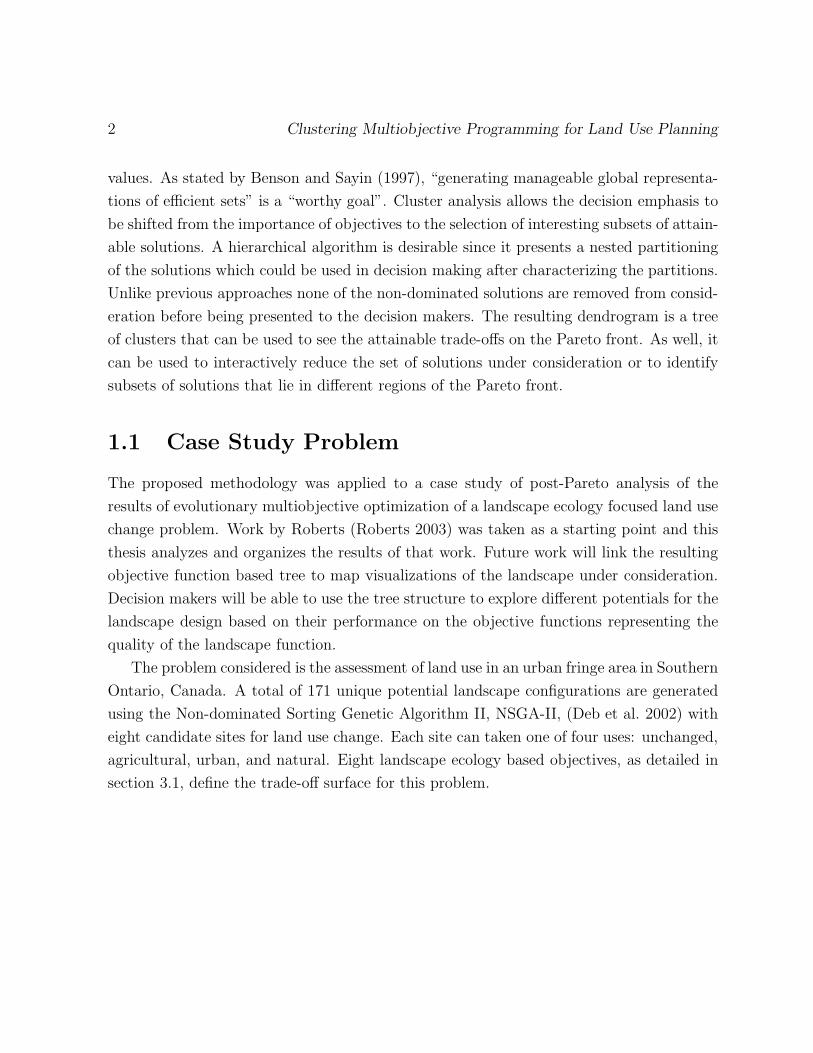
1.1 Case Study Problem
The proposed methodology was applied to a case study of post-Pareto analysis of the
results of evolutionary multiobjective optimization of a landscape ecology focused land use
change problem. Work by Roberts (Roberts 2003) was taken as a starting point and this
thesis analyzes and organizes the results of that work. Future work will link the resulting
objective function based tree to map visualizations of the landscape under consideration.
Decision makers will be able to use the tree structure to explore different potentials for the
landscape design based on their performance on the objective functions representing the
quality of the landscape function.
The problem considered is the assessment of land use in an urban fringe area in Southern
Ontario, Canada. A total of 171 unique potential landscape configurations are generated
using the Non-dominated Sorting Genetic Algorithm II, NSGA-II, (Deb et al. 2002) with
eight candidate sites for land use change. Each site can taken one of four uses: unchanged,
agricultural, urban, and natural. Eight landscape ecology based objectives, as detailed in
section 3.1, define the trade-off surface for this problem.
Introduction 3
1.2 Thesis Organization
This thesis begins with this short introduction in chapter 1. Chapter 2 contains a literature
review with background in multiobjective optimization, cluster analysis, and the land
use configuration problem. The literature review also establishes the current state of
the literature in multiobjective post-optimization analysis and planning decision support.
Chapter 4 describes the proposed cluster analysis methodology including preparation of
the data and selection of a relevant algorithm as well as also detailing the evaluation
methodology for the proposed analysis as well as three alternate data organization methods
for comparison. Chapter 5 applies the methodology described in section 4.1 and the three
comparable methods, considers the validity of the results, and gives an example of using the
results for a land use decision. Chapter 6 discusses these results and the suitability of the
proposed method for handling multiobjective optimization results. Chapter 7 summarizes
the results and discussion, delineates the implications and limitations of the proposed
methodology, and gives directions for future work.

Chapter 2
Literature Review and Background
This chapter reviews the relevant literature for this thesis including multiobjective op-
timization, land use planning, and cluster analysis. The methodology and assessment
methods are outlined in chapter 4. The remainder of this thesis applies the cluster analy-
sis methodology developed in chapter 4 and assesses it using the landscape configuration
optimization problem described in section 3.
This literature review begins with concepts and definitions from multiobjective opti-
mization. Solution schemes for multiobjective optimization problems with discussion of
their shortcomings follow. The Pareto optimization framework is described and previous
work in improving the output of Pareto optimization is discussed in section 2.2; this post-
Pareto analysis literature is the most relevant literature to the methodology described in
this thesis. The following section describes the landscape configuration optimization prob-
lem as formulated and solved by Roberts (2003) including two modifications. Material on
decision making in spatial problems is reviewed. A description of relevant cluster analysis
methods follows. This chapter concludes with a statement of the objective of this thesis.
2.1 Multiobjective Optimization
According to Rardin (1998): “When goals cannot be reduced to a common scale of cost
or benefit, trade-offs have [to] be addressed. Only a model with multiple objective func-
tions is satisfactory . . . ”. A multiobjective optimization problem is composed of a set of
5
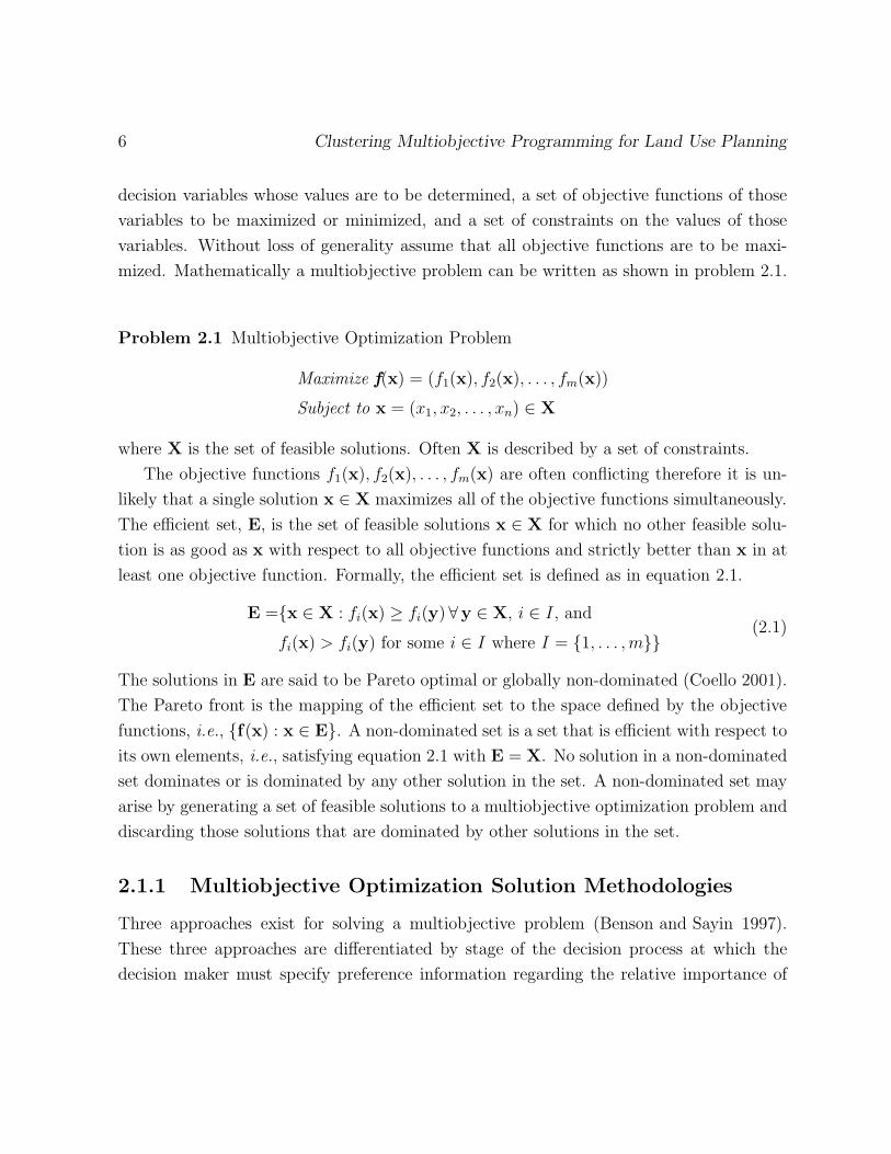
6 Clustering Multiobjective Programming for Land Use Planning
decision variables whose values are to be determined, a set of objective functions of those
variables to be maximized or minimized, and a set of constraints on the values of those
variables. Without loss of generality assume that all objective functions are to be maxi-
mized. Mathematically a multiobjective problem can be written as shown in problem 2.1.
Problem 2.1 Multiobjective Optimization Problem
Maximize f(x) = (f1(x), f2(x), . . . , fm(x))
Subject to x = (x1, x2, . . . , xn) ∈ X
where X is the set of feasible solutions. Often X is described by a set of constraints.
The objective functions f1(x), f2(x), . . . , fm(x) are often conflicting therefore it is un-
likely that a single solution x ∈ X maximizes all of the objective functions simultaneously.
The efficient set, E, is the set of feasible solutions x ∈ X for which no other feasible solu-
tion is as good as x with respect to all objective functions and strictly better than x in at
least one objective function. Formally, the efficient set is defined as in equation 2.1.
E ={x ∈ X : fi(x) ≥ fi(y) ∀y ∈ X, i ∈ I, and
fi(x) > fi(y) for some i ∈ I where I = {1, . . . , m}}(2.1)
The solutions in E are said to be Pareto optimal or globally non-dominated (Coello 2001).
The Pareto front is the mapping of the efficient set to the space defined by the objective
functions, i.e., {f(x) : x ∈ E}. A non-dominated set is a set that is efficient with respect to
its own elements, i.e., satisfying equation 2.1 with E = X. No solution in a non-dominated
set dominates or is dominated by any other solution in the set. A non-dominated set may
arise by generating a set of feasible solutions to a multiobjective optimization problem and
discarding those solutions that are dominated by other solutions in the set.
2.1.1 Multiobjective Optimization Solution Methodologies
Three approaches exist for solving a multiobjective problem (Benson and Sayin 1997).
These three approaches are differentiated by stage of the decision process at which the
decision maker must specify preference information regarding the relative importance of
Literature Review and Background 7
the objective functions differentiates. The first approach requires preferences to be spec-
ified a priori and entails reformulating the problem as a single objective problem. For
this approach preference information is required from the decision makers, e.g., relative
importance or weights of the objective functions, goal levels for the objective functions, or
values functions combining the objective functions. The second approach elicits preferences
throughout the optimization and requires that the decision makers interact with the opti-
mization procedure, typically by specifying preferences between presented solutions. The
third approach, known as Pareto optimization, finds a representative set of non-dominated
solutions approximating the Pareto front before requiring preference information from the
decision makers. Pareto optimization methods, such as evolutionary multiobjective opti-
mization algorithms, allow decision makers to investigate the candidate solutions without
a priori judgments regarding the relative importance of objective functions.
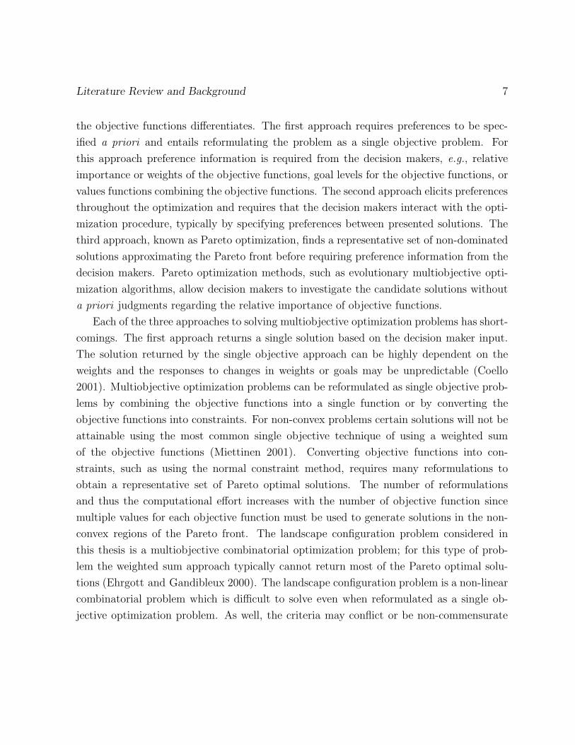
Each of the three approaches to solving multiobjective optimization problems has short-
comings. The first approach returns a single solution based on the decision maker input.
The solution returned by the single objective approach can be highly dependent on the
weights and the responses to changes in weights or goals may be unpredictable (Coello
2001). Multiobjective optimization problems can be reformulated as single objective prob-
lems by combining the objective functions into a single function or by converting the
objective functions into constraints. For non-convex problems certain solutions will not be
attainable using the most common single objective technique of using a weighted sum
of the objective functions (Miettinen 2001). Converting objective functions into con-
straints, such as using the normal constraint method, requires many reformulations to
obtain a representative set of Pareto optimal solutions. The number of reformulations
and thus the computational effort increases with the number of objective function since
multiple values for each objective function must be used to generate solutions in the non-
convex regions of the Pareto front. The landscape configuration problem considered in
this thesis is a multiobjective combinatorial optimization problem; for this type of prob-
lem the weighted sum approach typically cannot return most of the Pareto optimal solu-
tions (Ehrgott and Gandibleux 2000). The landscape configuration problem is a non-linear
combinatorial problem which is difficult to solve even when reformulated as a single ob-
jective optimization problem. As well, the criteria may conflict or be non-commensurate
8 Clustering Multiobjective Programming for Land Use Planning
making it difficult to make value judgments in choosing weights or goals for the criteria
(Greenwood et al. 1997). Even if these value judgments can be made the resulting math-
ematical formulation may be inconsistent or difficult to optimize (Miettinen 2001). The
second approach considers only a small set of non-dominated solutions due to the effort
required on the part of the decision makers (Benson and Sayin 1997). The third approach,
Pareto optimization, results in a potentially large number of solutions that must be con-
sidered. Selecting a single solution from a large non-dominated set is likely to be difficult
for decision makers. In addition, Pareto optimization approaches are typically more com-
putationally expensive than the first two approaches but they do not make the demands
on the decision maker required in the interactive approach.
Benson and Sayin (1997) proposed that an ideal solution procedure for multiobjective
optimization is to provide the decision maker(s) with a globally representative subset of the
non-dominated set that is sufficiently small so as to be tractable. We aim to approach that
ideal by accepting the computational effort required to generate a large non-dominated set
and subsequently organizing it using its own structure to allow decision makers to find and
consider interesting subsets without deleting any of the candidate solutions.
2.1.2 Evolutionary Multiobjective Algorithms
Evolutionary multiobjective algorithms are a subset of Pareto optimization methods that
apply biologically inspired evolutionary processes as heuristics to generate non-dominated
sets of solutions. A set of operators is applied to a population of solutions to generate
new solutions subject to evolutionary pressure to improve. It should be noted that these
solutions may not be Pareto optimal but the algorithms are designed to evolve solutions
that approach the Pareto front and that are sufficiently diverse to capture the spread of
solutions existing on the Pareto front. These methods are robust to the shape of the Pareto
front (Coello 2001).
The Non-dominated Sorting Genetic Algorithm (NSGA) used by Roberts (2003) to
solve the case study problem is replaced here with NSGA-II. Compared to NSGA, NSGA-
II has lower computation complexity, removes the need for a sharing parameter, and im-
plements elitism (Deb et al. 2002). The cluster analysis methodology presented in this
thesis can be employed with any Pareto optimization method if the resulting distribution
Literature Review and Background 9
of solutions is appropriate for hierarchical clustering. NSGA-II is used since it is known
to perform well with non-convex, disconnected, and non-uniform Pareto fronts (Deb et al.
2002). The results returned by NSGA-II are typically not a non-dominated set but are
composed of several non-domination fronts close to the true Pareto front. The use of this
heuristic algorithm allows for efficient searching of a large solution space based on several
discontinuous non-convex objective functions.
NSGA-II is a genetic algorithm (GA). GAs operate on a population of solutions and
employ selection, crossover, and mutation operators, among others, in order to generate
successive improved populations based on a fitness function. At each generation a set of
potential parents is generated, subsets of the parents are combined to create offspring, and
the fittest offspring are included in the next generation (Falkenauer 1998). NSGA-II differs
from single objective GAs in two respects: it aims to maintain diversity in the population
instead of converging to a single solution and it uses non-domination to assess the fitness of
individuals. These differences affect the generation of the set of parents and the selection of
the next generation. The fitness function used by NSGA-II is an artificial fitness; instead
of using the objective functions directly the fitness function is based on the dominance
relationships in the current population. Better fitness values are assigned to members of
the population that are dominated by fewer other members of the population.
At each generation, given a current population, Pt, with N members, the operations
of selection, crossover, and mutation are applied to create an offspring population, Qt,
with N members. The members of the population are represented by the chromosome
strings encoding the decision variables such as the scheme described in section 3. Elitism
is implemented in NSGA-II by allowing the members of the next generation to be drawn
from either the offspring, Qt, or the parents, Pt. Denoting the potential members of the
next generation as Rt, this implies that Rt = Pt∪Qt. The next population, Pt+1, is created
by sorting the potential members, Rt, according to non-domination and crowding distance
then using binary tournament selection based on this order favouring the better members.
The non-domination and crowding distance sorting can be summarized as preferring
the dominating solution if two solutions are on different fronts and preferring the solution
with the lower crowding distance if the solutions are on the same front. This sorting is
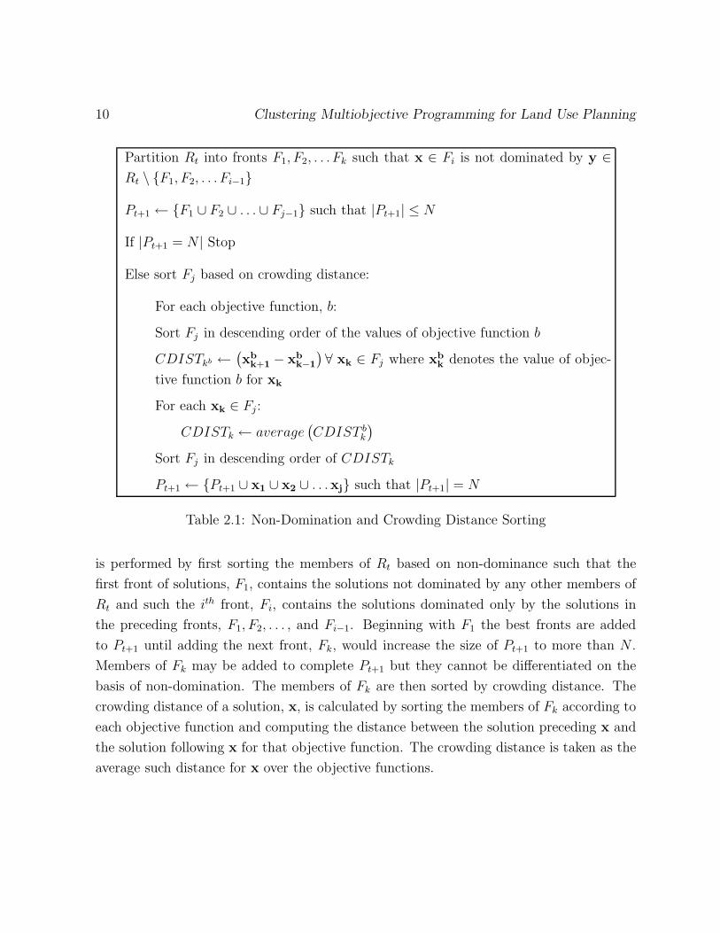
shown as pseudo-code in table 2.1. The non-domination and crowding distance sorting
10 Clustering Multiobjective Programming for Land Use Planning
Partition Rt into fronts F1, F2, . . . Fk such that x ∈ Fi is not dominated by y ∈Rt \ {F1, F2, . . . Fi−1}
Pt+1 ← {F1 ∪ F2 ∪ . . . ∪ Fj−1} such that |Pt+1| ≤ N
If |Pt+1 = N | Stop
Else sort Fj based on crowding distance:
For each objective function, b:
Sort Fj in descending order of the values of objective function b
CDISTkb ←(
xbk+1 − xb
k−1
)
∀ xk ∈ Fj where xbk denotes the value of objec-
tive function b for xk
For each xk ∈ Fj :
CDISTk ← average(
CDIST bk
)
Sort Fj in descending order of CDISTk
Pt+1 ← {Pt+1 ∪ x1 ∪ x2 ∪ . . .xj} such that |Pt+1| = N
Table 2.1: Non-Domination and Crowding Distance Sorting
is performed by first sorting the members of Rt based on non-dominance such that the
first front of solutions, F1, contains the solutions not dominated by any other members of
Rt and such the ith front, Fi, contains the solutions dominated only by the solutions in
the preceding fronts, F1, F2, . . . , and Fi−1. Beginning with F1 the best fronts are added
to Pt+1 until adding the next front, Fk, would increase the size of Pt+1 to more than N .
Members of Fk may be added to complete Pt+1 but they cannot be differentiated on the
basis of non-domination. The members of Fk are then sorted by crowding distance. The
crowding distance of a solution, x, is calculated by sorting the members of Fk according to
each objective function and computing the distance between the solution preceding x and
the solution following x for that objective function. The crowding distance is taken as the
average such distance for x over the objective functions.
Literature Review and Background 11
r
r
r
uu
u
uu
b
b
bb
f1(x)
f2(x)
r
u
b
Front 1Front 2Front 3
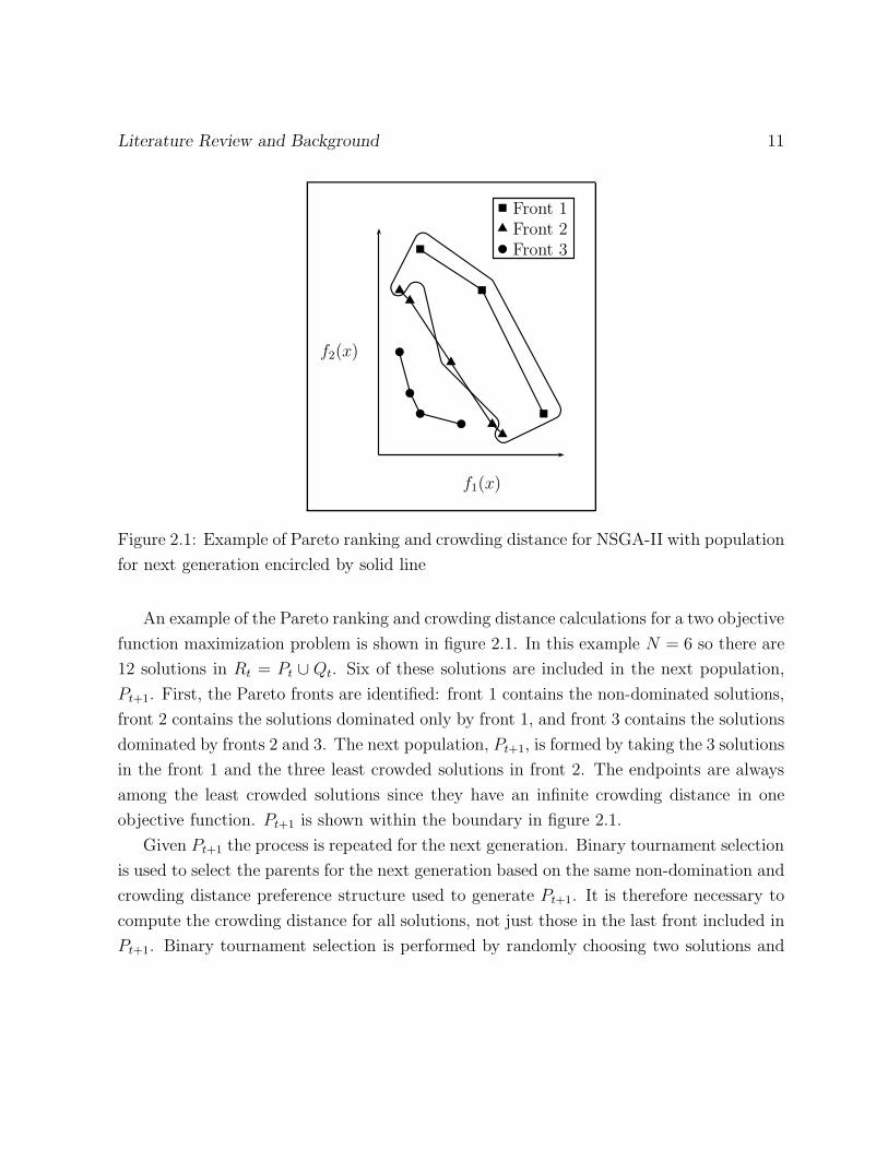
Figure 2.1: Example of Pareto ranking and crowding distance for NSGA-II with population
for next generation encircled by solid line
An example of the Pareto ranking and crowding distance calculations for a two objective
function maximization problem is shown in figure 2.1. In this example N = 6 so there are
12 solutions in Rt = Pt ∪ Qt. Six of these solutions are included in the next population,
Pt+1. First, the Pareto fronts are identified: front 1 contains the non-dominated solutions,
front 2 contains the solutions dominated only by front 1, and front 3 contains the solutions
dominated by fronts 2 and 3. The next population, Pt+1, is formed by taking the 3 solutions
in the front 1 and the three least crowded solutions in front 2. The endpoints are always
among the least crowded solutions since they have an infinite crowding distance in one
objective function. Pt+1 is shown within the boundary in figure 2.1.
Given Pt+1 the process is repeated for the next generation. Binary tournament selection
is used to select the parents for the next generation based on the same non-domination and
crowding distance preference structure used to generate Pt+1. It is therefore necessary to
compute the crowding distance for all solutions, not just those in the last front included in
Pt+1. Binary tournament selection is performed by randomly choosing two solutions and
12 Clustering Multiobjective Programming for Land Use Planning
including the higher ranked solution with a fixed probability typically between 0.5 and 1
(Goldberg and Deb 1991). The crossover operation used is single point crossover and the
mutation employed is site-wise mutation.
While the capability is not used in this thesis, NSGA-II can be modified to accom-
modate constraints on the decision variables. The constraint handling is performed by
extending the binary tournament selection operator to consider constraint violation in ad-
dition to dominance and crowding distance. Feasible solutions are most preferred, followed
by solutions with smaller constraint violation. Constraint violation can be measured by
normalizing the constraint function values and taking the sum of the violation magnitudes
for each constraint (Deb 2000). If both solutions selected for the binary tournament are
feasible then the selection is unchanged from that made by NSGA-II without constraint
handling.
2.2 Post-Pareto Analysis
Post-Pareto analysis concentrates on aiding the decision makers in choosing a final sin-
gle solution from the potentially large set generated by a Pareto optimization method.
Approaches taken include pruning the non-dominated set to the ‘most interesting’ solu-
tions and partitioning the non-dominated set into subsets of similar solutions. Several
researchers have applied clustering methods and distance-based methods to aid decision
makers in considering Pareto optimization results.
Most of these methods rely on considering the similarity of the elements of the non-
dominated set based on their objective function values and removing elements that are
deemed too similar to other elements. In this thesis a tree data structure is used to
organize the non-dominated set to allow decision makers to consider tractable subsets of
the non-dominated solutions without removing any of the elements.
Mattson et al. (2004) detailed a ‘smart Pareto filter’ to obtain a sufficiently small rep-
resentative subset of a non-dominated set. This method does not use cluster analysis.
The smart Pareto filtering approach defines regions of ‘practically insignificant trade-offs’
around points. Each point is considered successively and all points in its region of ‘prac-
tically insignificant trade-off’ are removed on the assumption that those points are not
Literature Review and Background 13
sufficiently distinguishable from the point under consideration. The representativeness re-
lies on retaining more elements of the non-dominated set to represent areas with steeper
trade-offs, commonly known as ‘knees’, and fewer elements to represent areas where the
elements are not highly distinguishable. Extremal solutions or solutions of high trade-off
are preserved as the non-dominated set is pruned. The smart Pareto filter requires the
specification of the dimensions of the regions of ‘practically insignificant trade-offs’ which
may differ for each objective function (Mattson et al. 2004). This specification requires the
decision makers to make a value judgment regarding what they perceive as similar without
first considering the potential values for each objective function and the magnitudes of the
trade-offs between the objective functions.
Greenwood et al. (1997) used a priori preferences from the decision makers to bias the
search of a GA. The preferences form part of the fitness function, in addition to the domi-
nance relation and the diversity mechanism. Fuzzy preferences are used to avoid aggregat-
ing non-commensurate objectives. Instead of approximating the entire Pareto front only
the subset of the Pareto front reflecting the preferences is approximated. Greenwood et al.
(1997) assumed that the preferences are consistent and do not vary across the solution
space; in other words, that the importance of a change in the value of an objective func-
tion does not depend on its current value or on the values of the other objective functions.
The shortcomings of specifying the preferences a priori apply; the decision makers are
not informed regarding the relationships between criteria or the attainable limits prior to
making value judgments.
Morse (1980) detailed one of the first applications of cluster analysis to a non-dominated
set. The multiobjective programs considered were linear programs. An element was re-
moved from the non-dominated set if there was another member of the non-dominated
set that was judged to be indistinguishable. Thresholds modelling the resolution of the
judgment of the decision maker were used to assess which solutions were indistinguishable.
Morse (1980) applied eight types of hierarchical clustering plus direct clustering, a naive
form of bi-clustering that groups both the solutions and the criteria defining the clusters, to
a problem with five objective functions and eight constraints. The hierarchical clustering
methods evaluated were single linkage, complete linkage, group average linkage, median
method, centroid method, Ward’s method, and McQuitty’s similarity analysis. Hierar-
14 Clustering Multiobjective Programming for Land Use Planning
chical clustering outperformed block clustering. In particular, Ward’s method, the group
average method, and the centroid method performed very well. The other five hierarchi-
cal clustering methods considered all exhibited an undesirable behaviour called chaining
which reduced the usefulness of the cluster structure obtained. Ward’s method was pre-
ferred since the clusters at the same level of the hierarchy were of similar size and shape.
Rosenman and Gero (1985) noted that the preference of Ward’s method by Morse (1980)
was based only on slightly better performance than centroid and group average methods
and that Ward’s method had other known shortcomings.
Rosenman and Gero (1985) applied complete linkage hierarchical clustering to ‘reduce
the size of the Pareto optimal set whilst retaining its shape’. Rosenman and Gero (1985)
noted that solutions whose vectors of objective function values are similar by an appro-
priate measure of proximity may have decision variable vectors that are similar or very
different; this idea was noted but not further explored. The aggregation of criteria implicit
in applying proximity measures to the objective function vectors of the elements of the
non-dominated set was avoided by considering the objective functions successively. The
complete linkage method was used since it allowed control of the diameter of the resulting
clusters. This method began by first clustering the elements of the non-dominated set
using a single criterion. Elements within the same cluster were then assumed to be indis-
tinguishable on this criterion. If a solution within a cluster dominated another solution
in that cluster on all criteria except the clustering criterion the dominated solution was
eliminated from consideration. The process was repeated for all criteria until the decision
makers decided that the non-dominated set was sufficiently small.
Taboada et al. (2007) used partitional (k-means) clustering for combinatorial multiob-
jective problems. Either the most interesting cluster, i.e., the ‘knee’ cluster, was considered
in detail by discarding the solutions in other clusters, or one solution from each of the k
clusters was considered to form a representative subset of the non-dominated set.
The Strength Pareto Evolutionary Algorithm (SPEA) proposed by Zitzler and Thiele
(1999) incorporates a clustering method in the optimization procedure. Unlike NSGA-II,
SPEA maintains an external elite population consisting of the best solutions found by the
algorithm so far. If this external population grows too large then it is pruned using cluster
analysis. Controlling the size of the external population is important for good algorithm
Literature Review and Background 15
performance in SPEA. The clustering algorithm employed is the average linkage method.
By retaining the centroid solutions in each cluster and removing some of the other solutions
in the clusters the cardinality of the external population can be reduced while retaining
its shape. The improvements to SPEA developed by Zitzler et al. (2001) and proposed as
SPEA2 include improving this pruning method to preserve extremal solutions.
This thesis differs from the above by considering hierarchical clustering and not reducing
the size of the non-dominated set under consideration before the solutions are presented to
the decision makers. As discussed in section 2.3, the complex and multi-participant nature
of land use decisions makes the presentation of similarly performing solutions desirable.
The hierarchical tree structure for the solutions allows the decision makers to tractably
consider the solutions using a sequence of decisions to reduce the set of solutions under
consideration. If a hierarchical structure is not suspected in the data or if the structure is
not to be used in the decision process then the methodology presented by Taboada et al.
(2007) may be more suitable.
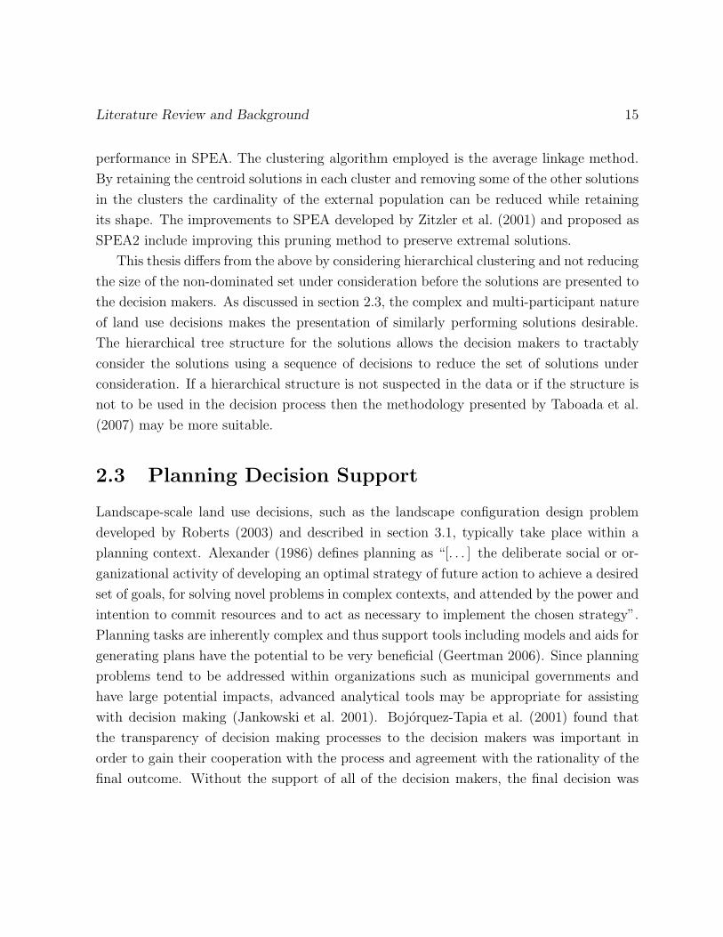
2.3 Planning Decision Support
Landscape-scale land use decisions, such as the landscape configuration design problem
developed by Roberts (2003) and described in section 3.1, typically take place within a
planning context. Alexander (1986) defines planning as “[. . . ] the deliberate social or or-
ganizational activity of developing an optimal strategy of future action to achieve a desired
set of goals, for solving novel problems in complex contexts, and attended by the power and
intention to commit resources and to act as necessary to implement the chosen strategy”.
Planning tasks are inherently complex and thus support tools including models and aids for
generating plans have the potential to be very beneficial (Geertman 2006). Since planning
problems tend to be addressed within organizations such as municipal governments and
have large potential impacts, advanced analytical tools may be appropriate for assisting
with decision making (Jankowski et al. 2001). Bojorquez-Tapia et al. (2001) found that
the transparency of decision making processes to the decision makers was important in
order to gain their cooperation with the process and agreement with the rationality of the
final outcome. Without the support of all of the decision makers, the final decision was
16 Clustering Multiobjective Programming for Land Use Planning
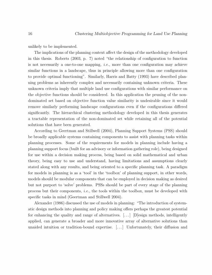
unlikely to be implemented.
The implications of the planning context affect the design of the methodology developed
in this thesis. Roberts (2003, p. 7) noted “the relationship of configuration to function
is not necessarily a one-to-one mapping, i.e., more than one configuration may achieve
similar functions in a landscape, thus in principle allowing more than one configuration
to provide optimal functioning”. Similarly, Harris and Batty (1993) have described plan-
ning problems as inherently complex and necessarily containing unknown criteria. These
unknown criteria imply that multiple land use configurations with similar performance on
the objective functions should be considered. In this application the pruning of the non-
dominated set based on objective function value similarity is undesirable since it would
remove similarly performing landscape configurations even if the configurations differed
significantly. The hierarchical clustering methodology developed in this thesis generates
a tractable representation of the non-dominated set while retaining all of the potential
solutions that have been generated.
According to Geertman and Stillwell (2004), Planning Support Systems (PSS) should
be broadly applicable systems containing components to assist with planning tasks within
planning processes. Some of the requirements for models in planning include having a
planning support focus (built for an advisory or information gathering role), being designed
for use within a decision making process, being based on solid mathematical and urban
theory, being easy to use and understand, having limitations and assumptions clearly
stated along with any results, and being oriented to a specific planning task. A paradigm
for models in planning is as a ‘tool’ in the ‘toolbox’ of planning support, in other words,
models should be modular components that can be employed in decision making as desired
but not purport to ‘solve’ problems. PSSs should be part of every stage of the planning
process but their components, i.e., the tools within the toolbox, must be developed with
specific tasks in mind (Geertman and Stillwell 2004).
Alexander (1986) discussed the use of models in planning: “The introduction of system-
atic design methods into planning and policy making offers perhaps the greatest potential
for enhancing the quality and range of alternatives. [. . . ] [D]esign methods, intelligently
applied, can generate a broader and more innovative array of alternative solutions than
unaided intuition or tradition-bound expertise. [. . . ] Unfortunately, their diffusion and
Literature Review and Background 17
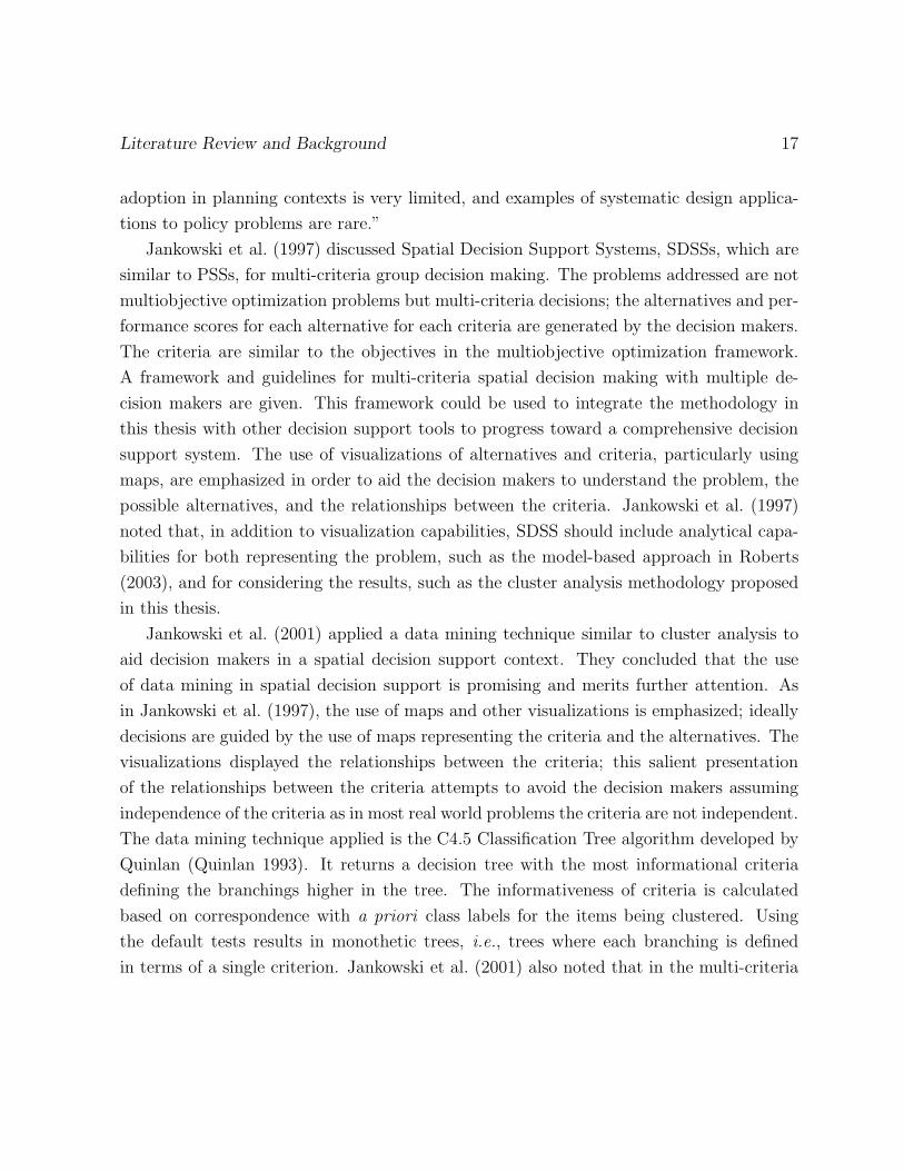
adoption in planning contexts is very limited, and examples of systematic design applica-
tions to policy problems are rare.”
Jankowski et al. (1997) discussed Spatial Decision Support Systems, SDSSs, which are
similar to PSSs, for multi-criteria group decision making. The problems addressed are not
multiobjective optimization problems but multi-criteria decisions; the alternatives and per-
formance scores for each alternative for each criteria are generated by the decision makers.
The criteria are similar to the objectives in the multiobjective optimization framework.
A framework and guidelines for multi-criteria spatial decision making with multiple de-
cision makers are given. This framework could be used to integrate the methodology in
this thesis with other decision support tools to progress toward a comprehensive decision
support system. The use of visualizations of alternatives and criteria, particularly using
maps, are emphasized in order to aid the decision makers to understand the problem, the
possible alternatives, and the relationships between the criteria. Jankowski et al. (1997)
noted that, in addition to visualization capabilities, SDSS should include analytical capa-
bilities for both representing the problem, such as the model-based approach in Roberts
(2003), and for considering the results, such as the cluster analysis methodology proposed
in this thesis.
Jankowski et al. (2001) applied a data mining technique similar to cluster analysis to
aid decision makers in a spatial decision support context. They concluded that the use
of data mining in spatial decision support is promising and merits further attention. As
in Jankowski et al. (1997), the use of maps and other visualizations is emphasized; ideally
decisions are guided by the use of maps representing the criteria and the alternatives. The
visualizations displayed the relationships between the criteria; this salient presentation
of the relationships between the criteria attempts to avoid the decision makers assuming
independence of the criteria as in most real world problems the criteria are not independent.
The data mining technique applied is the C4.5 Classification Tree algorithm developed by
Quinlan (Quinlan 1993). It returns a decision tree with the most informational criteria
defining the branchings higher in the tree. The informativeness of criteria is calculated
based on correspondence with a priori class labels for the items being clustered. Using
the default tests results in monothetic trees, i.e., trees where each branching is defined
in terms of a single criterion. Jankowski et al. (2001) also noted that in the multi-criteria
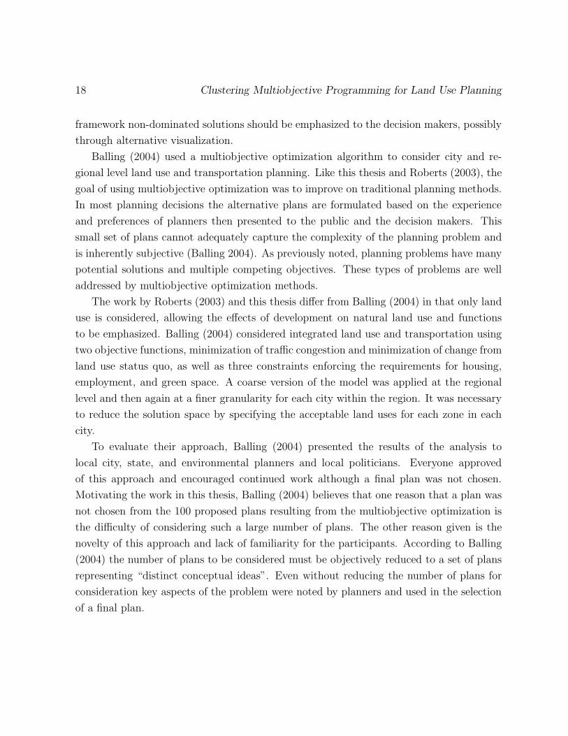
18 Clustering Multiobjective Programming for Land Use Planning
framework non-dominated solutions should be emphasized to the decision makers, possibly
through alternative visualization.
Balling (2004) used a multiobjective optimization algorithm to consider city and re-
gional level land use and transportation planning. Like this thesis and Roberts (2003), the
goal of using multiobjective optimization was to improve on traditional planning methods.
In most planning decisions the alternative plans are formulated based on the experience
and preferences of planners then presented to the public and the decision makers. This
small set of plans cannot adequately capture the complexity of the planning problem and
is inherently subjective (Balling 2004). As previously noted, planning problems have many
potential solutions and multiple competing objectives. These types of problems are well
addressed by multiobjective optimization methods.
The work by Roberts (2003) and this thesis differ from Balling (2004) in that only land
use is considered, allowing the effects of development on natural land use and functions
to be emphasized. Balling (2004) considered integrated land use and transportation using
two objective functions, minimization of traffic congestion and minimization of change from
land use status quo, as well as three constraints enforcing the requirements for housing,
employment, and green space. A coarse version of the model was applied at the regional
level and then again at a finer granularity for each city within the region. It was necessary
to reduce the solution space by specifying the acceptable land uses for each zone in each
city.
To evaluate their approach, Balling (2004) presented the results of the analysis to
local city, state, and environmental planners and local politicians. Everyone approved
of this approach and encouraged continued work although a final plan was not chosen.
Motivating the work in this thesis, Balling (2004) believes that one reason that a plan was
not chosen from the 100 proposed plans resulting from the multiobjective optimization is
the difficulty of considering such a large number of plans. The other reason given is the
novelty of this approach and lack of familiarity for the participants. According to Balling
(2004) the number of plans to be considered must be objectively reduced to a set of plans
representing “distinct conceptual ideas”. Even without reducing the number of plans for
consideration key aspects of the problem were noted by planners and used in the selection
of a final plan.
Literature Review and Background 19
2.4 Clustering Methods
The methodology proposed in this thesis for organizing multiobjective optimization results
used a hierarchical clustering algorithm to construct a tree of the solutions returned by
NSGA-II. This section discusses the relevant background material on clustering including
alternative approaches to which the proposed methodology will be compared. Cluster
analysis involves the use of algorithms and techniques to examine the internal organization
in a data set in an objective way; it can be used to describe the data concisely and to
uncover patterns and relationships that may not be readily apparent (Dubes 1993). The
aim is to group objects that are similar in some way.
Clustering methods are often separated into two categories: partitional methods which
provide a single partition of the solutions and hierarchical methods which provide a series
of nested partitions. A partition is an assignment of the elements to a set of clusters.
Typically each element is assigned to a single cluster. A significant element in the choice of a
clustering method is whether the nested structure from a hierarchical algorithm is useful or
desirable; such a structure cannot be derived from a partitional algorithm (Dubes and Jain
1979). An additional advantage of using a hierarchical clustering method is that the number
of clusters need not be known a priori (Ward 1963).
Many clustering methods assume an underlying model for the clusters (Halkidi et al.
2001), often hyperellipsoidal cluster shape or generation by a Gaussian distribution. Thus
different clustering algorithms are appropriate for different data sets (Jain et al. 1999).
It should be noted that although the choice of a clustering method is important there
remains significant freedom within a method to deliver varied results (Jain et al. 1999).
For example, data normalization and the selection of a similarity measure can significantly
affect the clustering results. The input of a subject matter expert in the application domain
is desirable; domain knowledge can be applied in clustering when representing the data,
selecting an appropriate measure of similarity, choosing a clustering method, and assessing
the validity of the results (Jain et al. 1999).
20 Clustering Multiobjective Programming for Land Use Planning
2.4.1 Partitional Clustering Algorithms
Partitional clustering methods, such as k-means clustering, make certain assumptions
about cluster properties (Karypis et al. 1999). These methods typically construct clus-
ters by minimizing a squared error criterion. Most often these methods assume that the
clusters are hyper ellipsoidal and sometimes assume underlying statistical processes, typ-
ically mixed Gaussian distributions. Mixed Gaussians exist when the data elements to
be clustered are generated from several different Gaussian distributions. Mixed Gaussians
can also be used when approximating non-Gaussian distributions. In cluster analysis the
data elements from each generation process are assumed to lie in different clusters. These
methods require the user to specify the number of clusters, k, a priori.
The most commonly applied partitional clustering algorithm is the k-means algorithm.
The k-means algorithm begins with k randomly chosen points as the representative centres
of k clusters (Jain et al. 1999). The clusters are formed by allocating each of the remaining
patterns to the nearest cluster. The cluster membership is re-evaluated by assigning each
point to the nearest cluster centroid and the locations of the centroids is recomputed.
This process is repeated iteratively until a stopping criterion is met. A typical stopping
criterion is no change in the allocation from the last iteration (Jain et al. 1999). K-means
is sensitive to the initial cluster centres, not guaranteed to attain the true globally optimal
partitional clustering, and has difficulty dealing with outliers due to the assumed hyper
ellipsoidal cluster model (Xu and Wunsch 2005).
Since partitional clustering algorithms cannot return the nested partition structure
required for the methodology developed in this thesis they are not considered further.
2.4.2 Hierarchical Clustering Algorithms
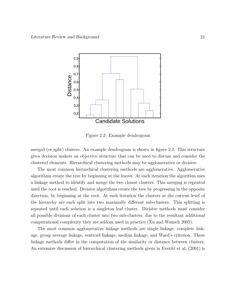
The tree structure of a hierarchical clustering algorithm can be useful for guiding decision
processes when many alternatives must be considered. The tree of the cluster hierarchy
is often represented in a dendrogram where the top element in the tree, the root, is a
cluster containing all of the elements and the bottom elements, i.e., the leaves, represent
individual elements. The dendrogram displays the merging (or dividing) of clusters from
the leaves to the root (or the root to the leaves) and the distance or dissimilarity between the
Literature Review and Background 21
0.2
0.3
0.4
0.5
0.6
0.7
0.8
0.9
Candidate Solutions
Dis
tanc
e
Figure 2.2: Example dendrogram
merged (or split) clusters. An example dendrogram is shown in figure 2.2. This structure
gives decision makers an objective structure that can be used to discuss and consider the
clustered elements. Hierarchical clustering methods may be agglomerative or divisive.
The most common hierarchical clustering methods are agglomerative. Agglomerative
algorithms create the tree by beginning at the leaves. At each iteration the algorithm uses
a linkage method to identify and merge the two closest clusters. This merging is repeated
until the root is reached. Divisive algorithms create the tree by progressing in the opposite
direction, by beginning at the root. At each iteration the clusters at the current level of
the hierarchy are each split into two maximally different sub-clusters. This splitting is
repeated until each solution is a singleton leaf cluster. Divisive methods must consider
all possible divisions of each cluster into two sub-clusters; due to the resultant additional
computational complexity they are seldom used in practice (Xu and Wunsch 2005).
The most common agglomerative linkage methods are single linkage, complete link-
age, group average linkage, centroid linkage, median linkage, and Ward’s criterion. These
linkage methods differ in the computation of the similarity or distance between clusters.
An extensive discussion of hierarchical clustering methods given in Everitt et al. (2001) is
22 Clustering Multiobjective Programming for Land Use Planning
summarized here. The single linkage computes the distance between clusters as the dis-
tance between the closest pair of elements with one element in each cluster, i.e., the nearest
neighbour distance. The complete linkage computes the distance between clusters as the
distance between the further elements with one element in each cluster, i.e., the furthest
neighbour distance. The group average linkage computes the distance between clusters as
the mean distance between all pairs with one element in the first cluster and one element
in the second cluster. The group average linkage may be weighted or unweighted; the
weighted group average linkage counts all pairs of elements including duplicate elements
whereas unweighted group average linkage considers only unique elements. Centroid link-
age computes the distance between clusters as the distance between the mean vectors of
the elements in each cluster. Median linkage computes the distance between clusters as
the distance between their mean vectors but weights the cluster based on the number of
elements in each cluster to avoid giving more implicit weight to larger clusters. Ward’s
method (Ward 1963) merges the clusters that minimize the within-cluster variance.
Hierarchical clustering linkage methods, like all clustering methods, often make as-
sumptions about the sizes and shapes of clusters (Jain et al. 1999). Each linkage tends to
find clusters with certain characteristics. The characteristics and assumptions of linkages
should be considered and compared with the data to be clustered in order to choose the
most appropriate approach. Single linkage can find clusters of varying sizes and shapes
but tends to produce long ‘chained’ clusters and can be sensitive to outliers as well as
the inclusion or deletion of single points (Karypis et al. 1999). Complete linkage tends to
generate compact clusters of the same size, i.e., balanced clusters. Group average linkage
allows clusters to vary in size and shape. Centroid linkage and median linkage assume
convex clusters of the same size and shape (Karypis et al. 1999). Centroid and median
linkages are subject to reversals; clusters may be joined with a smaller inter-cluster dis-
tance than the sub-clusters that were joined to create those clusters (Everitt et al. 2001).
A reversal creates a non-monotonic dendrogram and reduces the interpretability of the
cluster tree structure. Ward’s method is sensitive to outliers, tends to form clusters of the
same size, and tends to perform poorly if the clusters contain different numbers of elements
(Everitt et al. 2001).
Literature Review and Background 23
2.4.3 Other Clustering Algorithms
To assess the quality of the results returned by the proposed methodology several alterna-
tive clustering methods will be applied to the NSGA-II output data. These methods are
described in this section.
Chameleon
Chameleon, developed by Karypis et al. (1999), is an agglomerative hierarchical clustering
algorithm using a different means of measuring cluster similarity than the linkage methods.
This method was proposed to overcome the shortcoming of most clustering methods; it
avoids making assumptions regarding the cluster sizes, shapes, or densities by dynamically
modelling the clusters. It uses measures of connectivity and proximity in order to determine
which clusters to merge at each branching.
The tree of the hierarchical clustering resulting from Chameleon does not have individ-
ual solutions as leaves since the dynamic modelling requires a critical mass of elements in
each cluster considered for merging. There are three steps to the Chameleon algorithm.
First, Chameleon creates the k-nearest neighbour graph of the elements to be clustered.
In the k-nearest neighbour graph the elements to be clustered are the nodes and an edge
exists between two nodes if one of the nodes is one of the k most similar nodes to the other
node. Second, a graph partitioning algorithm partitions the k-nearest neighbour graph
into many small clusters. Third, Chameleon merges these small clusters based on two
criteria to generate a hierarchical clustering structure. The two merging criteria are the
relative interconnectivity and the relative closeness of the clusters (Karypis et al. 1999).
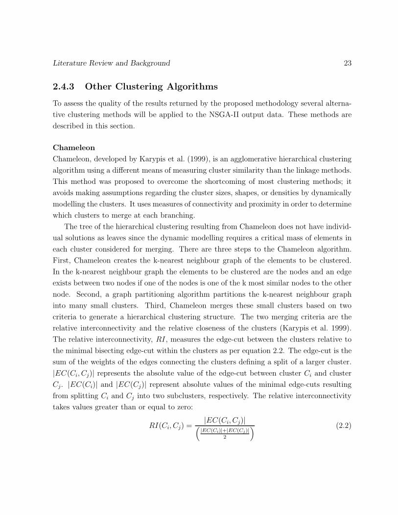
The relative interconnectivity, RI, measures the edge-cut between the clusters relative to
the minimal bisecting edge-cut within the clusters as per equation 2.2. The edge-cut is the
sum of the weights of the edges connecting the clusters defining a split of a larger cluster.
|EC(Ci, Cj)| represents the absolute value of the edge-cut between cluster Ci and cluster
Cj. |EC(Ci)| and |EC(Cj)| represent absolute values of the minimal edge-cuts resulting
from splitting Ci and Cj into two subclusters, respectively. The relative interconnectivity
takes values greater than or equal to zero:
RI(Ci, Cj) =|EC(Ci, Cj)|
(
|EC(Ci)|+|EC(Cj)|
2
) (2.2)
24 Clustering Multiobjective Programming for Land Use Planning
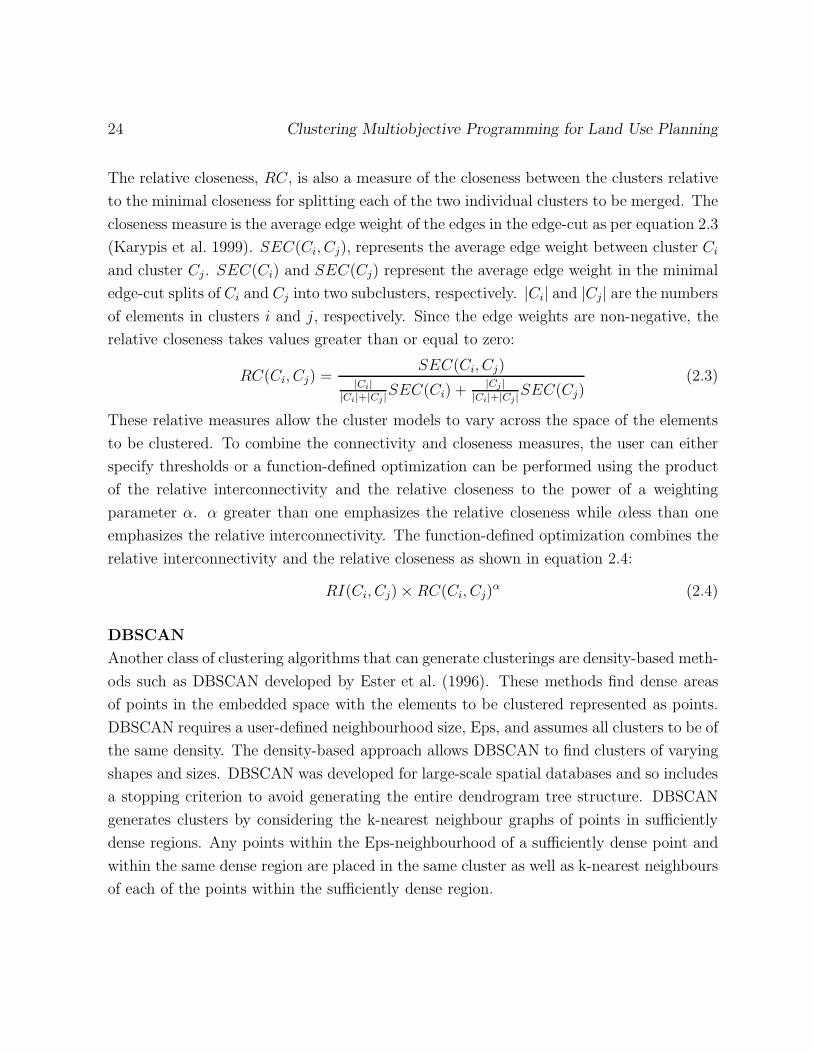
The relative closeness, RC, is also a measure of the closeness between the clusters relative
to the minimal closeness for splitting each of the two individual clusters to be merged. The
closeness measure is the average edge weight of the edges in the edge-cut as per equation 2.3
(Karypis et al. 1999). SEC(Ci, Cj), represents the average edge weight between cluster Ci
and cluster Cj . SEC(Ci) and SEC(Cj) represent the average edge weight in the minimal
edge-cut splits of Ci and Cj into two subclusters, respectively. |Ci| and |Cj| are the numbers
of elements in clusters i and j, respectively. Since the edge weights are non-negative, the
relative closeness takes values greater than or equal to zero:
RC(Ci, Cj) =SEC(Ci, Cj)
|Ci||Ci|+|Cj |
SEC(Ci) +|Cj |
|Ci|+|Cj |SEC(Cj)
(2.3)
These relative measures allow the cluster models to vary across the space of the elements
to be clustered. To combine the connectivity and closeness measures, the user can either
specify thresholds or a function-defined optimization can be performed using the product
of the relative interconnectivity and the relative closeness to the power of a weighting
parameter α. α greater than one emphasizes the relative closeness while αless than one
emphasizes the relative interconnectivity. The function-defined optimization combines the
relative interconnectivity and the relative closeness as shown in equation 2.4:
RI(Ci, Cj)× RC(Ci, Cj)α (2.4)
DBSCAN
Another class of clustering algorithms that can generate clusterings are density-based meth-
ods such as DBSCAN developed by Ester et al. (1996). These methods find dense areas
of points in the embedded space with the elements to be clustered represented as points.
DBSCAN requires a user-defined neighbourhood size, Eps, and assumes all clusters to be of
the same density. The density-based approach allows DBSCAN to find clusters of varying
shapes and sizes. DBSCAN was developed for large-scale spatial databases and so includes
a stopping criterion to avoid generating the entire dendrogram tree structure. DBSCAN
generates clusters by considering the k-nearest neighbour graphs of points in sufficiently
dense regions. Any points within the Eps-neighbourhood of a sufficiently dense point and
within the same dense region are placed in the same cluster as well as k-nearest neighbours
of each of the points within the sufficiently dense region.
Literature Review and Background 25
Decision Tree Classifiers
Like hierarchical clustering methods, decision tree classifiers construct hierarchical struc-
tures of the elements to be considered (Friedl and Brodley 1997). Decision tree classifiers
are similar to divisive hierarchical clustering algorithms as they begin by considering all of
the elements to be classified and successively splitting the elements into nested classes. This
approach differs from hierarchical clustering algorithms in the tests used to generate the
branchings. As classifiers, i.e., supervised learning algorithms in contrast to unsupervised
learning in clustering algorithms, decision tree classifiers use known classes for the objects
being clustered to determine the branchings. Basak and Krishnapuram (2005) proposed
a decision tree motivated clustering method that uses branching rules that do not require
class labels. Decision tree classifiers may be monothetic or polythetic. Monothetic classi-
fiers have branchings based on a single data feature. Most often the branching is binary
and splits the elements using a single objective function into two classes where one has
values greater than a threshold value and the other contains the elements with values less
than the threshold. The threshold value is selected to maximize a discriminant measure
such as the information gain. The resulting partitions of the feature space are separated by
hyperplanes that are parallel to the feature axes. Polythetic decision tree classifiers allow
the branchings to be based on tests of multiple features. Typically the tests are linear sums
of the features. The resulting feature space boundaries are hyperplanes but may not be
orthogonal to the feature axes. The additional complexity in determining the coefficients of
the features in polythetic decision trees makes them more sensitive to algorithmic choices
but often results in more compact trees than monothetic decision trees. Both of these types
of decision tree classifiers assume that the clusters are clearly separated by hyperplanes.
The complexities of Chameleon and DBSCAN make them unsuitable for use in practical
spatial decision support applications. However, these more complex methods make different
assumptions regarding the characteristics of the clusters; these methods are used to assess
the validity of the results returned using the proposed average linkage hierarchical clustering
methodology. If the simpler proposed method returns a similar or better cluster structure
than the more complex methods are not required for this application. If the results are
similar the cluster structure is more likely to be valid as it is robust to the assumptions
regarding the cluster characteristics. If the results differ than they must be compared

26 Clustering Multiobjective Programming for Land Use Planning
to determine which cluster structure is a more accurate representation of the solutions.
Decision tree classifiers make more restrictive assumptions regarding the tree branchings
than the hierarchical clustering algorithms and are expected to result in less informative
or less compact decision trees.
This chapter detailed the background necessary to develop the greenlands design prob-
lem of interest in this thesis. The literature reviewed includes multiobjective optimization,
decision support for planning problems, and cluster analysis methods. Chapter 3 describes
the problem of interest including previous work by Roberts (2003) and concludes with a
statement of the problem addressed in this thesis. Chapter 4 then describes the proposed
cluster analysis methodology, the alternative approaches, and the evaluation framework.
The remaining chapters apply these methods then present and discuss the results.
Chapter 3
Problem Statement
This chapter begins with a description of the greenlands problem formulated by Roberts
(2003) including the multiobjective optimization model. A description of the methodol-
ogy used to generate the potential solutions follows. This methodology is similar to the
methodology used in Roberts (2003) but uses the updated Non-dominated Sorting Ge-
netic Algorithm II (NSGA-II) in place of the Non-dominated Sorting Genetic Algorithm
(NSGA). The results of Roberts (2003) are described and the chapter concludes with a
statement of the problem addressed in this thesis.
The greenlands design problem detailed by Roberts (2003) concerns an urban fringe
area west of Toronto in Southern Ontario, Canada. In this region single family residential
housing and aggregate extraction (hereafter referred to collectively as urban), agriculture,
and natural areas co-exist. The analysis aims to inform land use decision making concerning
the effects of land use, in particular potential habitat loss and fragmentation represented
by reduction in the area and connectedness of natural land. The model takes into account
the existing landscape features and the existing land use. Currently abandoned fields could
potentially be used to allow for urban growth, re-seeded or allowed to regenerate as natural
areas to contribute to habitats, or restored as agricultural land. The configuration of the
landscape features is important in the evaluation of the land use.
27
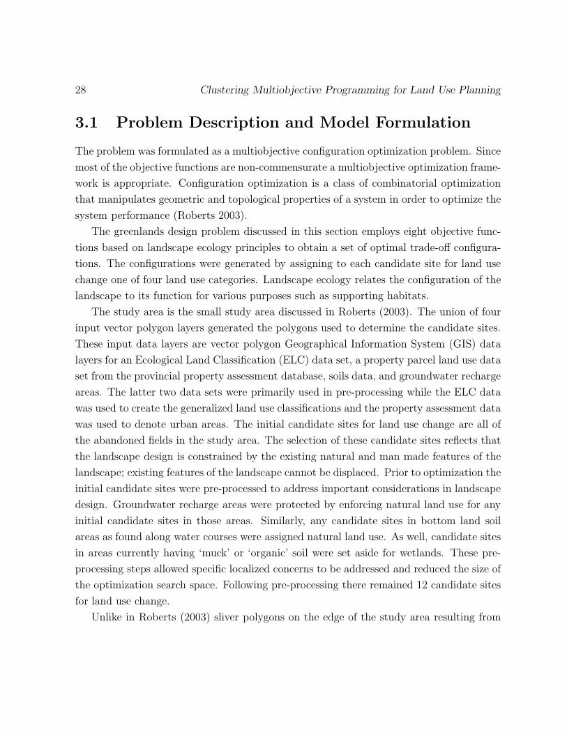
28 Clustering Multiobjective Programming for Land Use Planning
3.1 Problem Description and Model Formulation
The problem was formulated as a multiobjective configuration optimization problem. Since
most of the objective functions are non-commensurate a multiobjective optimization frame-
work is appropriate. Configuration optimization is a class of combinatorial optimization
that manipulates geometric and topological properties of a system in order to optimize the
system performance (Roberts 2003).
The greenlands design problem discussed in this section employs eight objective func-
tions based on landscape ecology principles to obtain a set of optimal trade-off configura-
tions. The configurations were generated by assigning to each candidate site for land use
change one of four land use categories. Landscape ecology relates the configuration of the
landscape to its function for various purposes such as supporting habitats.
The study area is the small study area discussed in Roberts (2003). The union of four
input vector polygon layers generated the polygons used to determine the candidate sites.
These input data layers are vector polygon Geographical Information System (GIS) data
layers for an Ecological Land Classification (ELC) data set, a property parcel land use data
set from the provincial property assessment database, soils data, and groundwater recharge
areas. The latter two data sets were primarily used in pre-processing while the ELC data
was used to create the generalized land use classifications and the property assessment data
was used to denote urban areas. The initial candidate sites for land use change are all of
the abandoned fields in the study area. The selection of these candidate sites reflects that
the landscape design is constrained by the existing natural and man made features of the
landscape; existing features of the landscape cannot be displaced. Prior to optimization the
initial candidate sites were pre-processed to address important considerations in landscape
design. Groundwater recharge areas were protected by enforcing natural land use for any
initial candidate sites in those areas. Similarly, any candidate sites in bottom land soil
areas as found along water courses were assigned natural land use. As well, candidate sites
in areas currently having ‘muck’ or ‘organic’ soil were set aside for wetlands. These pre-
processing steps allowed specific localized concerns to be addressed and reduced the size of
the optimization search space. Following pre-processing there remained 12 candidate sites
for land use change.
Unlike in Roberts (2003) sliver polygons on the edge of the study area resulting from
Problem Statement 29
small differences in the input data source polygons were removed (cf. Roberts and Calamai
(2007)). This step reduced the number of candidate sites to eight. The landscape config-
uration problem is combinatorial since it involves selecting one of four land use codes for
each of the candidate sites. This combinatorial structure results in significant additional
effort required to process each additional candidate site, therefore it is desirable to remove
sliver polygons. To remove sliver polygons they can be merged with one of their bordering
polygons on the edge of the study area. This merging can be done by users generating the
input data although it is more difficult than keeping the sliver polygons. Since the slivers
have little area this merging does not significantly affect the objective functions measuring
the percentage of the area assigned to each land use area. If the sliver is on the edge of the
study area then it is unlikely that this merging will affect the connectivity of the natural
areas or the joins between natural or natural and urban sites, particularly since most of
the slivers border only one other polygon. No objective functions are significantly affected
by the removal of sliver polygons at the edge of the study area. If the sliver is in the
centre of the study area then merging it into one of its bordering polygons could change
the adjacency relationships between its bordering polygons and affect all of the objective
functions except the land use area objective functions. For example, a sliver polygon may
be required to connect two core natural areas to form a large contiguous natural area.
A third possibility exists in addition to merging the slivers and keeping the slivers. An
alternative representation of the polygon boundaries, e.g., fuzzy boundaries, can be used to
avoid changing the adjacency relationships while reducing the number of candidate sites.
This approach requires additional processing of the input data to transform it into the
alternative representation; the user will not be able to directly use their GIS data as input.
The candidate sites are represented by polygons on the landscape; these polygons were
created by overlaying the input source data maps to create a partition of the landscape
into polygons of land with known attributes. These candidate sites are shown in gray on
the study area map in figure 3.1.
Once the candidate sites and their boundaries were defined, the generalized land use
classes were modelled using categorical decision variables. The categories were aggre-
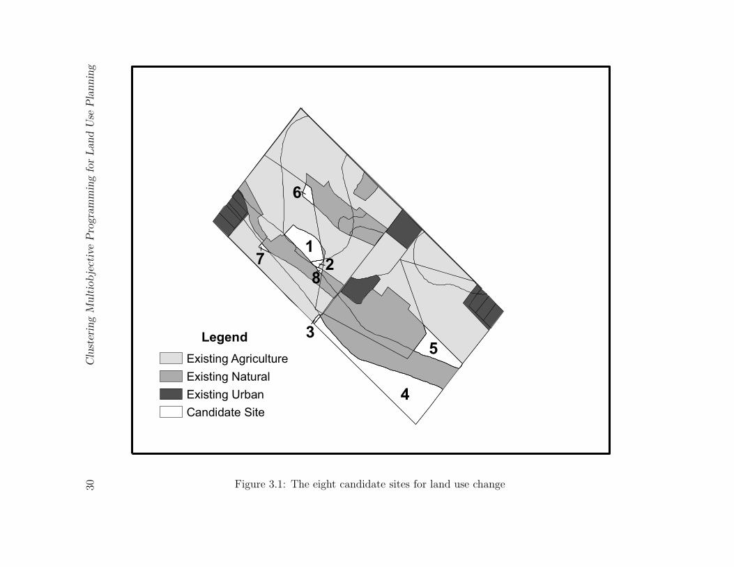
30C
lust
erin
gM
ult
iobje
ctiv
eP
rogra
mm
ing
for
Land
Use
Pla
nnin
g
4
5
1
6
27
3
8
Legend
Existing Agriculture
Existing Natural
Existing Urban
Candidate Site
Figure 3.1: The eight candidate sites for land use change
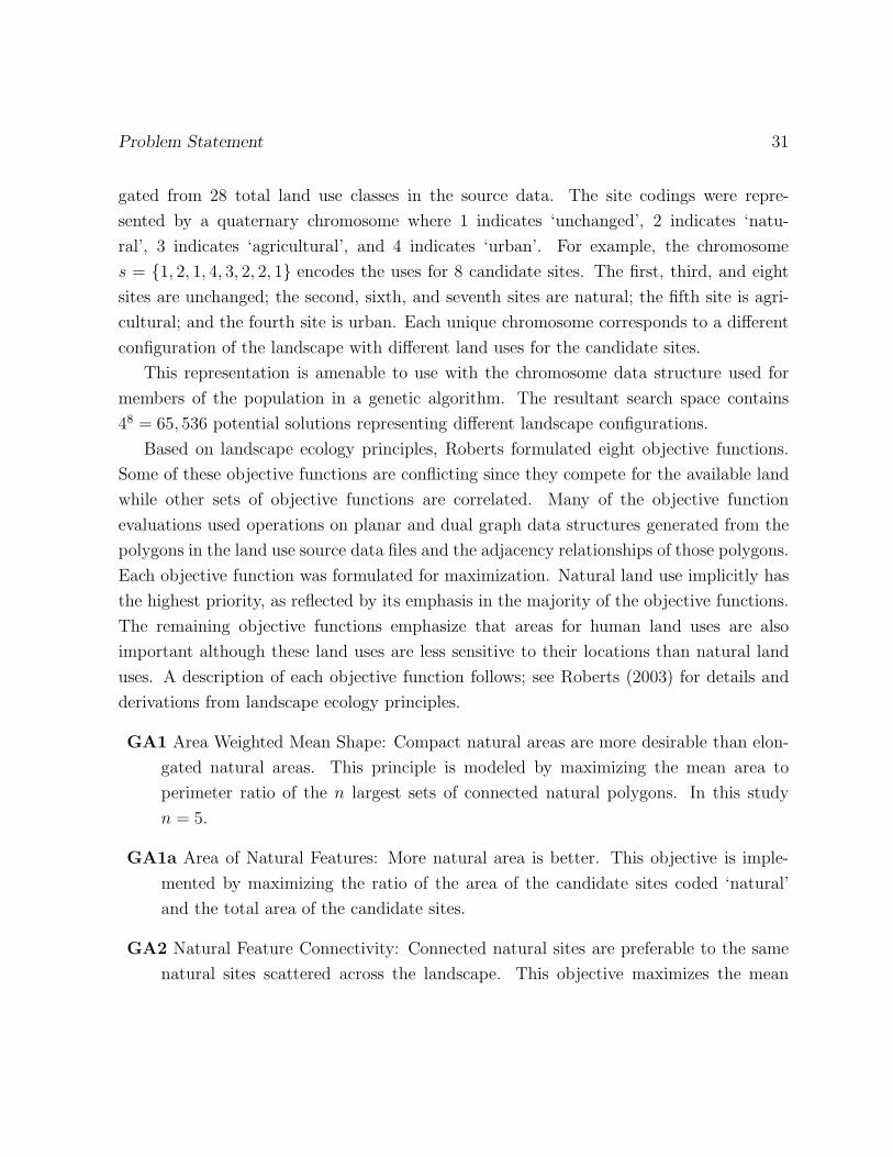
Problem Statement 31
gated from 28 total land use classes in the source data. The site codings were repre-
sented by a quaternary chromosome where 1 indicates ‘unchanged’, 2 indicates ‘natu-
ral’, 3 indicates ‘agricultural’, and 4 indicates ‘urban’. For example, the chromosome
s = {1, 2, 1, 4, 3, 2, 2, 1} encodes the uses for 8 candidate sites. The first, third, and eight
sites are unchanged; the second, sixth, and seventh sites are natural; the fifth site is agri-
cultural; and the fourth site is urban. Each unique chromosome corresponds to a different
configuration of the landscape with different land uses for the candidate sites.
This representation is amenable to use with the chromosome data structure used for
members of the population in a genetic algorithm. The resultant search space contains
48 = 65, 536 potential solutions representing different landscape configurations.
Based on landscape ecology principles, Roberts formulated eight objective functions.
Some of these objective functions are conflicting since they compete for the available land
while other sets of objective functions are correlated. Many of the objective function
evaluations used operations on planar and dual graph data structures generated from the
polygons in the land use source data files and the adjacency relationships of those polygons.
Each objective function was formulated for maximization. Natural land use implicitly has
the highest priority, as reflected by its emphasis in the majority of the objective functions.
The remaining objective functions emphasize that areas for human land uses are also
important although these land uses are less sensitive to their locations than natural land
uses. A description of each objective function follows; see Roberts (2003) for details and
derivations from landscape ecology principles.
GA1 Area Weighted Mean Shape: Compact natural areas are more desirable than elon-
gated natural areas. This principle is modeled by maximizing the mean area to
perimeter ratio of the n largest sets of connected natural polygons. In this study
n = 5.
GA1a Area of Natural Features: More natural area is better. This objective is imple-
mented by maximizing the ratio of the area of the candidate sites coded ‘natural’
and the total area of the candidate sites.
GA2 Natural Feature Connectivity: Connected natural sites are preferable to the same
natural sites scattered across the landscape. This objective maximizes the mean
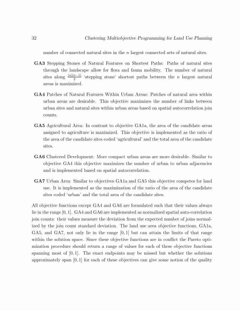
32 Clustering Multiobjective Programming for Land Use Planning
number of connected natural sites in the n largest connected sets of natural sites.
GA3 Stepping Stones of Natural Features on Shortest Paths: Paths of natural sites
through the landscape allow for flora and fauna mobility. The number of natural
sites along (n)(n−1)2
‘stepping stone’ shortest paths between the n largest natural
areas is maximized.
GA4 Patches of Natural Features Within Urban Areas: Patches of natural area within
urban areas are desirable. This objective maximizes the number of links between
urban sites and natural sites within urban areas based on spatial autocorrelation join
counts.
GA5 Agricultural Area: In contrast to objective GA1a, the area of the candidate areas
assigned to agriculture is maximized. This objective is implemented as the ratio of
the area of the candidate sites coded ‘agricultural’ and the total area of the candidate
sites.
GA6 Clustered Development: More compact urban areas are more desirable. Similar to
objective GA4 this objective maximizes the number of urban to urban adjacencies
and is implemented based on spatial autocorrelation.
GA7 Urban Area: Similar to objectives GA1a and GA5 this objective competes for land
use. It is implemented as the maximization of the ratio of the area of the candidate
sites coded ‘urban’ and the total area of the candidate sites.
All objective functions except GA4 and GA6 are formulated such that their values always
lie in the range [0, 1]. GA4 and GA6 are implemented as normalized spatial auto-correlation
join counts: their values measure the deviation from the expected number of joins normal-
ized by the join count standard deviation. The land use area objective functions, GA1a,
GA5, and GA7, not only lie in the range [0, 1] but can attain the limits of that range
within the solution space. Since these objective functions are in conflict the Pareto opti-
mization procedure should return a range of values for each of these objective functions
spanning most of [0, 1]. The exact endpoints may be missed but whether the solutions
approximately span [0, 1] for each of these objectives can give some notion of the quality
Problem Statement 33
of the approximation to the true Pareto front. This observation was used in determining
an appropriate population size and number of generations for NSGA-II.
In Roberts (2003) and in this thesis all potential solutions represented by the chro-
mosomal encoding were assumed to be feasible. In other words, any candidate site could
feasibly be assigned any of the four land use categories. The feasibility of the solutions
returned by the optimization procedure could be assessed after examining the solutions or,
in future implementations, could be explicitly modelled as constraints in the optimization
model. As noted in section 2.1.2, NSGA-II can be applied to constrained multiobjective
optimization problems (Deb et al. 2002) although that capability was not used in this the-
sis as information regarding the suitability of each site for each land use was unavailable.
As well, it is more informative to consider all possibilities since it may be possible to con-
vert unsuitable sites for certain land uses to suitable sites. In a real world decision process,
the capability of NSGA-II to handle constraints would be used to represent the suitable
land uses for each site based on information from the stakeholders.
3.2 Solution Methodology
The multiobjective landscape configuration design problem was solved using an evolu-
tionary multiobjective optimization algorithm. In the context of Pareto optimization
‘solved’ denotes the generation of a range of solutions approximating the true Pareto front
(Miettinen 2001). Landscape configurations whose objective function values approached
the Pareto front were evolved using the Non-dominated Sorting Genetic Algorithm II
(NSGA-II) developed by Deb et al. (2002). NSGA-II is described in section 2.1.2. The set
of solutions returned must be further examined by the decision makers in order to select
a solution; this process may involve considering additional constraints or objective func-
tions not included in this model but can be completed after the decision makers have been
informed about the attainable limits and the trade-offs between the objective functions.
34 Clustering Multiobjective Programming for Land Use Planning
3.3 Results and Conclusions
Roberts (2003) found the multiobjective optimization approach described above tended
to produce landscape configurations that reflected the importance of the natural features
while maintaining some diversity in the population of solutions. The small study area
restricted the impact of some objective functions. For example, even if all candidate sites
were allocated to natural land use the two largest pre-existing natural areas could not
be joined. While this may have been evident from the area map it was clearly shown in
the optimization results and in the two larger study areas considered in Roberts (2003)
such constraints may not be at all obvious. As well, the small study area contains few
urban areas and few candidate sites adjacent to these urban areas. Thus the clustered
development objective function, GA6, could be only marginally improved.
In the small population used due to computational limitations and the goals of the
study in Roberts (2003), most of the final solutions were very similar. The methodology
proposed in this thesis requires a larger and more varied population of solutions as it aims
to consider an approximation of the entire spectrum of optimal trade-off solutions instead
of finding a set of good designs taking into account the implicit land use priorities.
3.4 Problem Statement
The aim of this thesis is to consider a hierarchical clustering approach to post-Pareto
analysis for discrete non-linear multiobjective optimization problems in order to obtain a
tractable representation of the non-dominated set under consideration. Pareto optimization
is desirable for many multiobjective problems since it allows the decision makers to consider
the possible objective function trade-offs before making value judgments. Unfortunately
the number of solutions returned for consideration from Pareto optimization can be too
large to be tractably considered by the decision makers. Previous post-Pareto methods
entail eliminating some of the elements of the non-dominated set before presenting the
set to decision makers. This approach is unnecessary and inappropriate if the distribution
of the elements of the Pareto front is non-uniform. The landscape configuration problem
formulated by Roberts (2003) described in section 3.1 is used as an example of such a

Problem Statement 35
problem. The use of this problem implies that concerns particular to spatial decision
making in a planning context must be considered.
The work presented in this thesis does not consider preferences, goals, or constraints al-
though these problem aspects could be included at the alternative generation stage instead
of using unconstrained NSGA-II. It is expected that in a real world decision context the
problem would be iteratively refined to align with the decision makers’ mental constructs
of the problem and to reflect the available data. This refinement could include goal levels
or constraints limiting the objective function values and reducing the size of the solution
space.
Chapter 4 outlines the proposed cluster analysis methodology, alternative approaches,
and the evaluation framework. Chapter 5 applies the methods and presents the results.
Subsequent chapters discuss and assess these results.
Chapter 4
Methodology
This chapter begins by developing the proposed cluster analysis methodology using a de-
scription of the input data, then discussing data scaling, proximity calculation, and selec-
tion and application of a clustering algorithm to a problem. Methodologies for applying
three comparable clustering methods discussed in the literature review for comparison
to the proposed methodology follow as well as the validity assessment methodology for
evaluation of the proposed methodology.
4.1 Proposed Methodology
Cluster analysis is a sub-field of exploratory data analysis, in contrast to traditional sta-
tistical methods for confirming or rejecting hypotheses about data. No a priori expected
model for the data is necessary for cluster analysis (Dubes 1993). Before applying a clus-
tering algorithm the data must be prepared to remove the potential for biases due to the
scale and representation of the data. As well, a proximity measure must be chosen to
quantify the differences between the elements to be clustered, in this case the different
objective function vectors of the landscape configurations returned by the optimization.
36
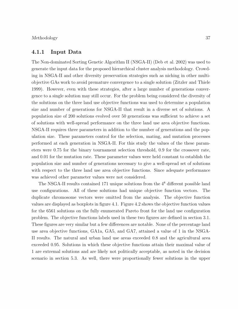
Methodology 37
4.1.1 Input Data
The Non-dominated Sorting Genetic Algorithm II (NSGA-II) (Deb et al. 2002) was used to
generate the input data for the proposed hierarchical cluster analysis methodology. Crowd-
ing in NSGA-II and other diversity preservation strategies such as niching in other multi-
objective GAs work to avoid premature convergence to a single solution (Zitzler and Thiele
1999). However, even with these strategies, after a large number of generations conver-
gence to a single solution may still occur. For the problem being considered the diversity of
the solutions on the three land use objective functions was used to determine a population
size and number of generations for NSGA-II that result in a diverse set of solutions. A
population size of 200 solutions evolved over 50 generations was sufficient to achieve a set
of solutions with well-spread performance on the three land use area objective functions.
NSGA-II requires three parameters in addition to the number of generations and the pop-
ulation size. These parameters control for the selection, mating, and mutation processes
performed at each generation in NSGA-II. For this study the values of the these param-
eters were 0.75 for the binary tournament selection threshold, 0.9 for the crossover rate,
and 0.01 for the mutation rate. These parameter values were held constant to establish the
population size and number of generations necessary to give a well-spread set of solutions
with respect to the three land use area objective functions. Since adequate performance
was achieved other parameter values were not considered.
The NSGA-II results contained 171 unique solutions from the 48 different possible land
use configurations. All of these solutions had unique objective function vectors. The
duplicate chromosome vectors were omitted from the analysis. The objective function
values are displayed as boxplots in figure 4.1. Figure 4.2 shows the objective function values
for the 6561 solutions on the fully enumerated Pareto front for the land use configuration
problem. The objective functions labels used in these two figures are defined in section 3.1.
These figures are very similar but a few differences are notable. None of the percentage land
use area objective functions, GA1a, GA5, and GA7, attained a value of 1 in the NSGA-
II results. The natural and urban land use areas exceeded 0.8 and the agricultural area
exceeded 0.95. Solutions in which these objective functions attain their maximal value of
1 are extremal solutions and are likely not politically acceptable, as noted in the decision
scenario in section 5.3. As well, there were proportionally fewer solutions in the upper
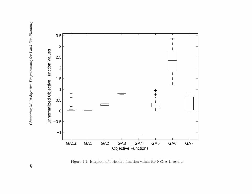
38C
lust
erin
gM
ult
iobje
ctiv
eP
rogra
mm
ing
for
Land
Use
Pla
nnin
g
GA1a GA1 GA2 GA3 GA4 GA5 GA6 GA7
−1
−0.5
0
0.5
1
1.5
2
2.5
3
3.5
Unn
orm
aliz
ed O
bjec
tive
Fun
ctio
n V
alue
s
Objective Functions
Figure 4.1: Boxplots of objective function values for NSGA-II results
Meth
odolo
gy
39
GA1a GA1 GA2 GA3 GA4 GA5 GA6 GA7
−1
−0.5
0
0.5
1
1.5
2
2.5
3
3.5
Unn
orm
aliz
ed O
bjec
tive
Fun
ctio
n V
alue
s
Objective Functions
Figure 4.2: Boxplots of objective function values for full enumeration of the true Pareto front
40 Clustering Multiobjective Programming for Land Use Planning
portions of the ranges for the natural and agricultural land use objective functions, GA1a
and GA5, respectively. The mean value for the urban land use objective function, GA7,
was higher in the NSGA-II results than in the enumeration of the true Pareto front. While
the ranges of new area for each land use were well represented in the NSGA-II results,
there is a bias toward urban land use and away from natural and agricultural land use.
The mean for GA2, the connectivity of natural area, was near the bottom of the range in
the NSGA-II results and near the top of the range in the Pareto front enumeration. There
were proportionally more solutions near the top and bottom of the range for GA6, clustered
development, in the NSGA-II results than the Pareto front enumeration. Objective GA4,
patches of natural features in urban areas, took only a single value in all of these results
due to the small problem size and the existing land use configuration, therefore it was
excluded from further analysis.
The input data was represented as a matrix, X, containing the data features for each
element to be clustered. In this case these features were the objective function values
for each Pareto optimal landscape configuration. The n rows of X represented the n
landscape configurations represented by the chromosome vectors returned by NSGA-II.
The p columns of X represented the objective function values. Thus entry xij of X was
the jth objective function value for proposed landscape configuration i. The elements to
be clustered can be envisioned as n points embedded in a p-dimensional space.
Since the decision variables were categorical, the true Pareto front and the approxima-
tions returned by NSGA-II were discrete sets of solutions. Due to this discreteness and
the non-linearity of some of the objective functions the density of the solutions was not
homogeneous across the Pareto front. This variation in solution density implies that a
hierarchical clustering structure may exist.
4.1.2 Clustering Tendency, Data Preparation, and Scaling
Cluster analysis should begin by checking the data for clustering tendency. If no such
tendency is found then any clustering of the data should not be considered valid, although
a dissection of the data using a clustering methodology may be useful (Dubes and Jain
1979). A visual inspection of the scatter plots of each pair of objective functions shown in
figure 4.3 was considered to establish the existence of hierarchical clustering in the NSGA-II
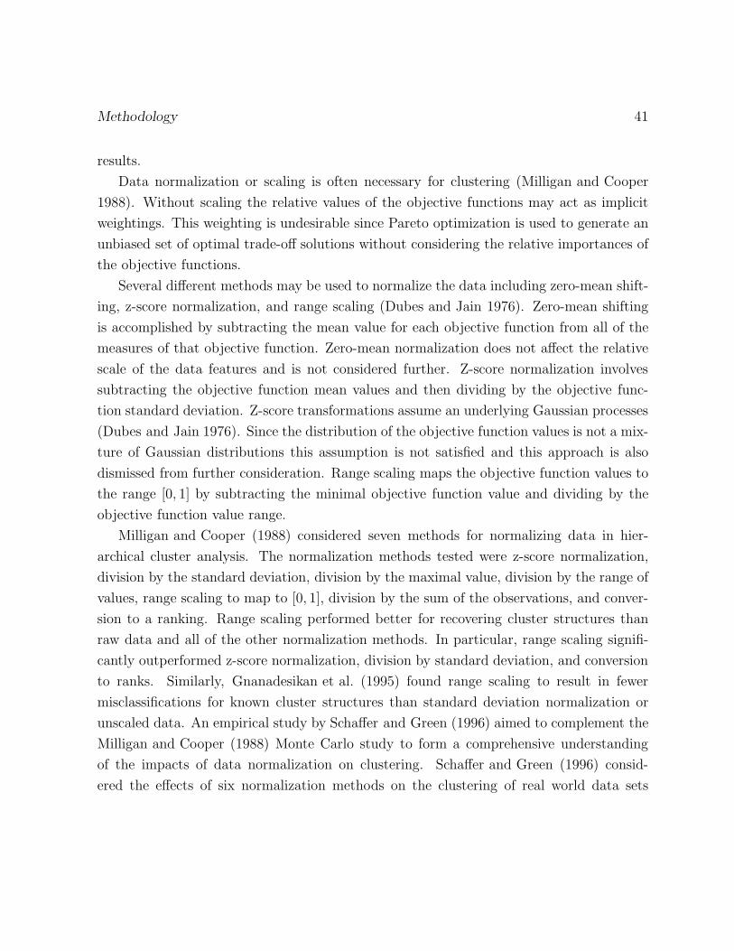
Methodology 41
results.
Data normalization or scaling is often necessary for clustering (Milligan and Cooper
1988). Without scaling the relative values of the objective functions may act as implicit
weightings. This weighting is undesirable since Pareto optimization is used to generate an
unbiased set of optimal trade-off solutions without considering the relative importances of
the objective functions.
Several different methods may be used to normalize the data including zero-mean shift-
ing, z-score normalization, and range scaling (Dubes and Jain 1976). Zero-mean shifting
is accomplished by subtracting the mean value for each objective function from all of the
measures of that objective function. Zero-mean normalization does not affect the relative
scale of the data features and is not considered further. Z-score normalization involves
subtracting the objective function mean values and then dividing by the objective func-
tion standard deviation. Z-score transformations assume an underlying Gaussian processes
(Dubes and Jain 1976). Since the distribution of the objective function values is not a mix-
ture of Gaussian distributions this assumption is not satisfied and this approach is also
dismissed from further consideration. Range scaling maps the objective function values to
the range [0, 1] by subtracting the minimal objective function value and dividing by the
objective function value range.
Milligan and Cooper (1988) considered seven methods for normalizing data in hier-
archical cluster analysis. The normalization methods tested were z-score normalization,
division by the standard deviation, division by the maximal value, division by the range of
values, range scaling to map to [0, 1], division by the sum of the observations, and conver-
sion to a ranking. Range scaling performed better for recovering cluster structures than
raw data and all of the other normalization methods. In particular, range scaling signifi-
cantly outperformed z-score normalization, division by standard deviation, and conversion
to ranks. Similarly, Gnanadesikan et al. (1995) found range scaling to result in fewer
misclassifications for known cluster structures than standard deviation normalization or
unscaled data. An empirical study by Schaffer and Green (1996) aimed to complement the
Milligan and Cooper (1988) Monte Carlo study to form a comprehensive understanding
of the impacts of data normalization on clustering. Schaffer and Green (1996) consid-
ered the effects of six normalization methods on the clustering of real world data sets
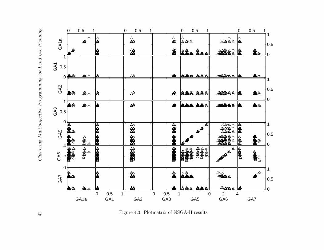
42C
lust
erin
gM
ult
iobje
ctiv
eP
rogra
mm
ing
for
Land
Use
Pla
nnin
g
0
0.5
1
GA70 2 4
GA6
GA50 0.5 1
GA3
GA20 0.5 1
GA1
GA1a
GA
7
0
2
4
GA
6
0
0.5
1
GA
5
0
0.5
1
GA
3
0
0.5
1
GA
2
0
0.5
1G
A1
0 0.5 1
0
0.5
10 0.5 10 0.5 10 0.5 1
GA
1a
Figure 4.3: Plotmatrix of NSGA-II results
Methodology 43
using k-means clustering. The normalization procedures were the same as those used by
Milligan and Cooper (1988) with a trimmed range method included and the division by
standard deviation excluded. The trimmed range method is similar to the range scaling
method but excludes the top and bottom 5% of the variable values when calculating the
range. The clustering results with normalization were compared to the k-means results
on the raw data and to several background attributes not included in the analysis. This
step is similar to typical tests of external cluster validity as discussed in section 4.1.6. In
contrast to Milligan and Cooper (1988), Schaffer and Green (1996) found that clustering
based on the raw data performed best. This difference may be a result of using the k-
means partitional clustering algorithm or indicate a lack of noise in the data, since the raw
data performed well in Milligan and Cooper (1988) other than when significant noise was
present. As in Milligan and Cooper (1988) other elements of a clustering study were seen
to be more significant than the effects of normalization, particularly the choice of clustering
method and the type and amount of noise in the raw data.
In addition to the scaling of the results there may be scaling issues implicit in the
Pareto optimization algorithm. In order to calculate the crowding distance in NSGA-II
the side lengths of cuboids each containing only a single solution must be computed. These
values are used in conjunction with the Pareto ranks in the crowded-comparison operator.
Deb et al. (2002) notes that each objective function must be normalized before computing
the crowding distance. This normalization uses linear range scaling to the range of values
for the objective function in the current generation. NSGA uses a sharing mechanism
instead of crowding that also included an implicit combination of objective functions;
the sharing parameter defined a neighbourhood around each solution and the fitness of a
solution was shared with any other solution in its neighbourhood. This neighbourhood can
be defined using any distance measure but has the same width along all of the objective
functions.
Range scaling was employed in this thesis to remove the implicit relative weights of
the objective functions in the NSGA-II results. All but one of the objective functions
were formulated to range [0, 1]. Only the spatial autocorrelation objective functions, GA4
and GA6, were not formulated to lie in this range. As noted above, since GA4 took only
a single value it was excluded from further analysis. Objective function GA6, clustered
44 Clustering Multiobjective Programming for Land Use Planning
development, was rescaled to lie in the range [0, 1] by mapping the lowest value occurring
in the NSGA-II results to 0 and the highest value occurring to 1 and linearly adjusting all
other values accordingly. Theoretically each objective function could have attained a value
of 1 within the solution space although the existing landscape configuration limited some
objective functions to a narrow range of values as seen in figure 4.1. The scaling within
NSGA-II was not considered and the Euclidean distance was used in the crowding distance
calculation; although it could have been modified to use the known limits for the objective
functions, the algorithm was applied as described in Deb et al. (2002).
4.1.3 Proximity
For most clustering methods part of preparing for cluster analysis, in addition to data
normalization, is obtaining a representative proximity measure (Jain and Dubes 1988).
The most common measures are symmetric and real-valued; in particular the Euclidean
distance is frequently used (Cormack 1971). Some reasons for the common use of the
Euclidean distance include ease of interpretability, particularly when using visualizations,
and invariance to rotations and translations. Many other metrics are possible, depending
on the type of data and the application.
Similarity measures include the Minkowski norms (which include the Euclidean and
rectilinear distances), the angular separation (or cosine metric), the correlation, the Can-
berra metric, and the Jaccard and simple matching metrics for binary categorical data
(Cormack 1971). Some metrics cannot easily accommodate correlated variables. The
Mahalanobis distance adjusts for the correlation between variables by incorporating the
covariance matrix (Cormack 1971). The Mahalanobis distance between two vectors x and
y with covariance matrix S is given by dM(x, y) =√
(x− y)TS−1(x− y). If the covariance
matrix is the identity matrix, i.e., the variables are independent, then the Mahalanobis
distance reduces to the Euclidean distance (Cormack 1971). The Mahalanobis distance
imposes a single model for all clusters; it assumes a single covariance matrix S over the
entire domain of the elements to be clustered (Mimmack et al. 2001). This assumption
is inappropriate if the correlation between the variables varies between clusters, i.e., if
the clusters have different shapes. The Mahalanobis can adapt to different correlations
in different regions if local covariance matrices are available. For the land configuration
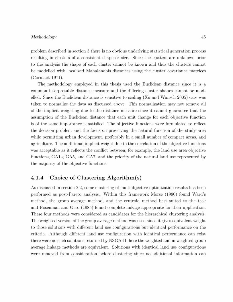
Methodology 45
problem described in section 3 there is no obvious underlying statistical generation process
resulting in clusters of a consistent shape or size. Since the clusters are unknown prior
to the analysis the shape of each cluster cannot be known and thus the clusters cannot
be modelled with localized Mahalanobis distances using the cluster covariance matrices
(Cormack 1971).
The methodology employed in this thesis used the Euclidean distance since it is a
common interpretable distance measure and the differing cluster shapes cannot be mod-
elled. Since the Euclidean distance is sensitive to scaling (Xu and Wunsch 2005) care was
taken to normalize the data as discussed above. This normalization may not remove all
of the implicit weighting due to the distance measure since it cannot guarantee that the
assumption of the Euclidean distance that each unit change for each objective function
is of the same importance is satisfied. The objective functions were formulated to reflect
the decision problem and the focus on preserving the natural function of the study area
while permitting urban development, preferably in a small number of compact areas, and
agriculture. The additional implicit weight due to the correlation of the objective functions
was acceptable as it reflects the conflict between, for example, the land use area objective
functions, GA1a, GA5, and GA7, and the priority of the natural land use represented by
the majority of the objective functions.
4.1.4 Choice of Clustering Algorithm(s)
As discussed in section 2.2, some clustering of multiobjective optimization results has been
performed as post-Pareto analysis. Within this framework Morse (1980) found Ward’s
method, the group average method, and the centroid method best suited to the task
and Rosenman and Gero (1985) found complete linkage appropriate for their application.
These four methods were considered as candidates for the hierarchical clustering analysis.
The weighted version of the group average method was used since it gives equivalent weight
to those solutions with different land use configurations but identical performance on the
criteria. Although different land use configuration with identical performance can exist
there were no such solutions returned by NSGA-II; here the weighted and unweighted group
average linkage methods are equivalent. Solutions with identical land use configurations
were removed from consideration before clustering since no additional information can
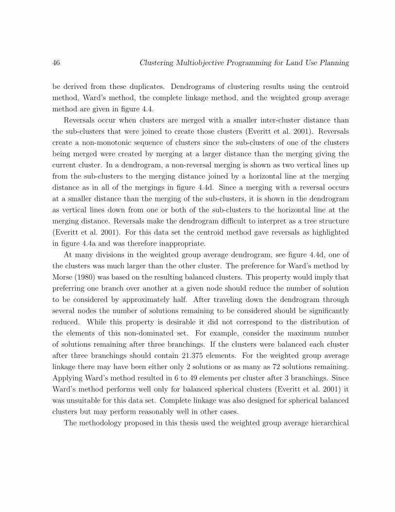
46 Clustering Multiobjective Programming for Land Use Planning
be derived from these duplicates. Dendrograms of clustering results using the centroid
method, Ward’s method, the complete linkage method, and the weighted group average
method are given in figure 4.4.
Reversals occur when clusters are merged with a smaller inter-cluster distance than
the sub-clusters that were joined to create those clusters (Everitt et al. 2001). Reversals
create a non-monotonic sequence of clusters since the sub-clusters of one of the clusters
being merged were created by merging at a larger distance than the merging giving the
current cluster. In a dendrogram, a non-reversal merging is shown as two vertical lines up
from the sub-clusters to the merging distance joined by a horizontal line at the merging
distance as in all of the mergings in figure 4.4d. Since a merging with a reversal occurs
at a smaller distance than the merging of the sub-clusters, it is shown in the dendrogram
as vertical lines down from one or both of the sub-clusters to the horizontal line at the
merging distance. Reversals make the dendrogram difficult to interpret as a tree structure
(Everitt et al. 2001). For this data set the centroid method gave reversals as highlighted
in figure 4.4a and was therefore inappropriate.
At many divisions in the weighted group average dendrogram, see figure 4.4d, one of
the clusters was much larger than the other cluster. The preference for Ward’s method by
Morse (1980) was based on the resulting balanced clusters. This property would imply that
preferring one branch over another at a given node should reduce the number of solution
to be considered by approximately half. After traveling down the dendrogram through
several nodes the number of solutions remaining to be considered should be significantly
reduced. While this property is desirable it did not correspond to the distribution of
the elements of this non-dominated set. For example, consider the maximum number
of solutions remaining after three branchings. If the clusters were balanced each cluster
after three branchings should contain 21.375 elements. For the weighted group average
linkage there may have been either only 2 solutions or as many as 72 solutions remaining.
Applying Ward’s method resulted in 6 to 49 elements per cluster after 3 branchings. Since
Ward’s method performs well only for balanced spherical clusters (Everitt et al. 2001) it
was unsuitable for this data set. Complete linkage was also designed for spherical balanced
clusters but may perform reasonably well in other cases.
The methodology proposed in this thesis used the weighted group average hierarchical
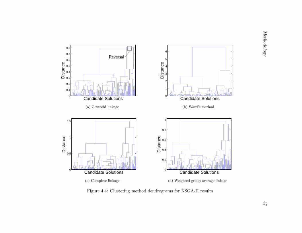
Meth
odolo
gy
47
0
0.1
0.2
0.3
0.4
0.5
0.6
0.7
0.8
Candidate Solutions
Dis
tanc
eReversal
(a) Centroid linkage
0
1
2
3
4
5
6
Candidate Solutions
Dis
tanc
e
(b) Ward’s method
0
0.5
1
1.5
Candidate Solutions
Dis
tanc
e
(c) Complete linkage
0
0.2
0.4
0.6
0.8
1
Candidate Solutions
Dis
tanc
e
(d) Weighted group average linkage
Figure 4.4: Clustering method dendrograms for NSGA-II results
48 Clustering Multiobjective Programming for Land Use Planning
clustering. Agreement with the complete linkage method was taken as an indicator of
cluster validity.
4.1.5 Application of Clustering Algorithm(s)
The weighted group average hierarchical clustering algorithm was applied to the normalized
data using the Euclidean proximity measure. The results of the hierarchical clustering
method were reported using a dendrogram to represent the hierarchy and parallel axis
plots or plotmatrices of the objective function values of the solutions in each cluster.
The hierarchical clustering algorithm was applied by using the Statistical Toolbox for
MATLAB to apply the algorithm shown in table 4.1. After reading in the NSGA-II results
as a matrix and removing solutions with identical land use configurations, the pdist func-
tion was used to compute the Euclidean distance between the objective function vectors
represented as the rows of the input data matrix in step 1. Then the linkage function
was used to merge the closest clusters in steps 2 and 3 and compute the distance between
clusters using the ’weighted’ method for the weighted average linkage and the ’complete’
method for the complete linkage in step 4. Finally the dendrogram function was used
to generate the dendrogram figures to display the results in step 5. Step 6 repeats the
merging process until all of the clusters have been merged into a single large cluster.
4.1.6 Validation
Since clustering methods will find clusters even in random data the validation of clustering
results is difficult. No absolute measure of cluster validity exists although validity indices
may be used to assist in assessing cluster validity (Halkidi et al. 2001). The structure found
must be assessed to determine whether the clustering is truly representative of the data,
including whether the data has any structure whatsoever (Gordon 1987). The final use of
the results should be considered; a comprehensive statistical assessment is not necessary if
the cluster results are to be simply a convenient summarization of the data. While measures
and tests of cluster validity can provide some indication of the validity of the output, the
best measure of cluster validity may be to consider the results in terms of expert knowledge
of the application (Jain et al. 1999). In any case, some objective assessment of the cluster
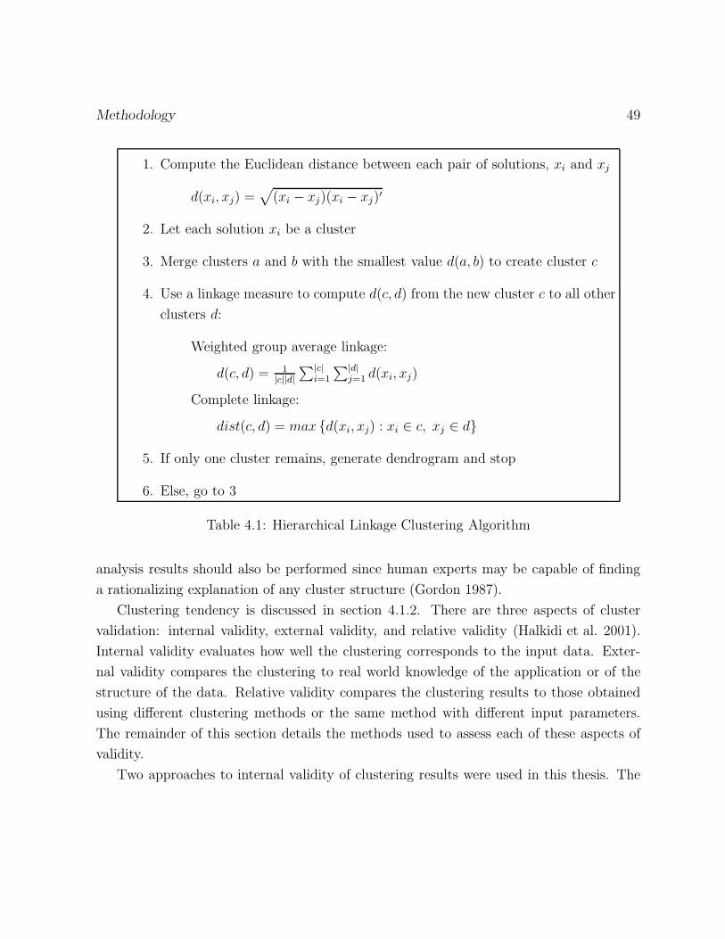
Methodology 49
1. Compute the Euclidean distance between each pair of solutions, xi and xj
d(xi, xj) =√
(xi − xj)(xi − xj)′
2. Let each solution xi be a cluster
3. Merge clusters a and b with the smallest value d(a, b) to create cluster c
4. Use a linkage measure to compute d(c, d) from the new cluster c to all other
clusters d:
Weighted group average linkage:
d(c, d) = 1|c||d|
∑|c|i=1
∑|d|j=1 d(xi, xj)
Complete linkage:
dist(c, d) = max {d(xi, xj) : xi ∈ c, xj ∈ d}
5. If only one cluster remains, generate dendrogram and stop
6. Else, go to 3
Table 4.1: Hierarchical Linkage Clustering Algorithm
analysis results should also be performed since human experts may be capable of finding
a rationalizing explanation of any cluster structure (Gordon 1987).
Clustering tendency is discussed in section 4.1.2. There are three aspects of cluster
validation: internal validity, external validity, and relative validity (Halkidi et al. 2001).
Internal validity evaluates how well the clustering corresponds to the input data. Exter-
nal validity compares the clustering to real world knowledge of the application or of the
structure of the data. Relative validity compares the clustering results to those obtained
using different clustering methods or the same method with different input parameters.
The remainder of this section details the methods used to assess each of these aspects of
validity.
Two approaches to internal validity of clustering results were used in this thesis. The
50 Clustering Multiobjective Programming for Land Use Planning
first approach was to consider the fit of a cluster hierarchy to the proximity matrix. The
cophenetic correlation coefficient (CCPC) is the most common measure of cluster hierarchy
fit (Dubes and Jain 1979). The CCPC measures the correlation of the distances between
the input data points and the cophenetic matrix derived from the dendrogram using the
product-moment correlation. Each entry, ci,j, of the cophenetic matrix is the level of the
hierarchy at which elements i and y are first in the same cluster, i.e., the birth height
of the cluster containing i and j. The CCPC is calculated using equation 4.1 where n is
the number of elements to be clustered, dij is the entry corresponding to elements i and
j in the proximity matrix, and cij is the entry corresponding to elements i and j in the
cophenetic matrix (Dubes and Jain 1979).
CCPC =(1/N)
∑
dijcij − dc
[(1/N)∑
d2ij − d
2]1
2 [(1/N)∑
c2ij − c2]
1
2
(4.1)
where, N = n(n − 1)/2, d = (1/N)∑
dij , and c = (1/N)∑
cij . All summations are over
all values of i and j where i < j. Dubes and Jain (1979) noted that a CCPC greater than
0.8 indicates a high degree of agreement between the proximity and cophenetic matrices
although the exact value lacks interpretability since it is influenced by the choice of clus-
tering algorithm, proximity measure, and the whether the proximity matrix is ultrametric.
A proximity matrix is ultrametric if it satisfies equation 4.2 (Dubes and Jain 1979).
dij ≤ max(dik, dkj) ∀(i, j, k) (4.2)
The second approach used to assess interval validity is data perturbation or stability
testing. This approach entails modifying the input data in some way and comparing the
results to the original clustering (Gordon 1987). The cluster structure should be robust
to reasonably small changes. Three stability tests are employed; in each case the data
was modified and the cluster analysis was repeated. Each test was repeated 5 times for
each set of input parameters. The first stability test was performed by adding random
perturbation terms to the objective function values. These random perturbations were
uniformly distributed with a mean of 0.5 and a width of 0.05, 0.10, and 0.25, corresponding
to 5%, 10%, and 25% of the potential range for the objective function values. The second
stability test was performed by removing some of the NSGA-II results from the objective
Methodology 51
function matrix. 5%, 10%, and 25% of the data points were removed and the cluster
analysis was repeated. The third stability test was performed by dividing the data set into
approximately two halves by randomly assigning each member to one of two subsets.
The external validity was assessed by comparing the cluster structure to the landscape
configurations. This external validation is similar to having a subject matter expert assess
the results in terms of their applicability to the decision. The most significant component
of the decision is the trade-off between the natural, agricultural, and urban land uses; the
cluster structure should reflect that trade-off and it should be clear from the landscape
configurations for the solutions in each cluster that this trade-off has implications for
the landscape designs. The landscape configurations corresponding to clusters were also
considered to determine whether the cluster analysis makes clear the effects of candidate
sites for particular objective functions.
Relative validity was also considered. Dubes and Jain (1979) recommended applying
multiple clustering algorithms and taking agreement in the results as an indicator of a
valid cluster structure. Parts of the structure that are similar with different clustering
methods likely indicate true structure in the data since the cluster models in the different
clustering algorithms will differ. Since the underlying models and assumptions for the
group average and complete linkage methods are significantly different, their agreement,
where it exists, was taken as an indicator of a valid cluster structure. As well, in this
thesis the dendrograms resulting from alternate clustering algorithms were compared to
the chosen clustering method to assess the robustness of the uncovered structure to the
clustering algorithm selection.
4.2 Comparable Methods
The alternative methods applied for comparison to the proposed methodology are described
in section 2.4.3. These methods were Chameleon, DBSCAN, and a binary monothetic
decision tree method. In spatial decision support overly complex analysis methodologies
are akin to black boxes; the understanding of the methodology by the decision makers
is essential to their cooperation during the analysis and the implementation of the final
results.
52 Clustering Multiobjective Programming for Land Use Planning
Chameleon is an example of a more complex clustering algorithm using the k-nearest
neighbour graph and dynamic cluster models. Chameleon was implemented using the
hMetis package (http://glaros.dtc.umn.edu/gkhome/) and Matlab based on Karypis et al.
(1999) and to partition the k-nearest neighbour graph and to find the optimal edge cuts in
the computations of the relative interconnectivity and closeness. Chameleon was applied
using a value of k = 15 for the k-nearest neighbour graph. The k value was increased from
10 used in Karypis et al. (1999) in order to obtain a connected k-nearest neighbour graph.
The connectivity of the k-nearest neighbour graph is necessary to obtain a single tree
structure when merging the partitions. The edge weights of the k-nearest neighbour graph
were computed as 1 − normalized Euclidean distance. The k-nearest neighbour graph is
partitioned into 16 subgraphs. A value of 2 was used for α, as in Karypis et al. (1999), to
emphasize the relative closeness over the relative interconnectivity.
DBSCAN represents an entirely different approach to clustering than the hierarchical
clustering methods; instead of considering the proximity of the elements to be clusters
DBSCAN uncovers clusters that are dense regions in the solution space. The Matlab code
for DBSCAN was obtained from http://www.chemometria.us.edu.pl/ (Daszykowski et al.
2001; 2002). In order to construct a hierarchical clustering DBSCAN was applied iter-
atively: first on the root, then on the resulting subclusters, and so on. DBSCAN uses
two parameters, k, the number of other elements that must be in the neighbourhood of
the current point to consider it a dense area, and Eps, the distance defining the neigh-
bourhood around a point. Eps was approximated using equation 4.3 where x is the data
matrix containing the objective function values, Γ is the gamma function, n is the num-
ber of objective function, i.e., columns in the data matrix, and k is as is described above
(Ester et al. 1996).
Eps =
[∏
(max(x)−min(x)) k Γ(0.5n + 1)
m√
πn
]1
n
(4.3)
DBSCAN was applied with Eps determined by the formula unless only a single cluster
resulted and k = 3. If only a single cluster resulted the value of Eps was changed to return
two clusters. If more than two clusters resulted using the automated value for Eps then
the branching split the current node into the resulting number of clusters. k values greater
than 4 require more computation and do not significantly improve the quality of the results
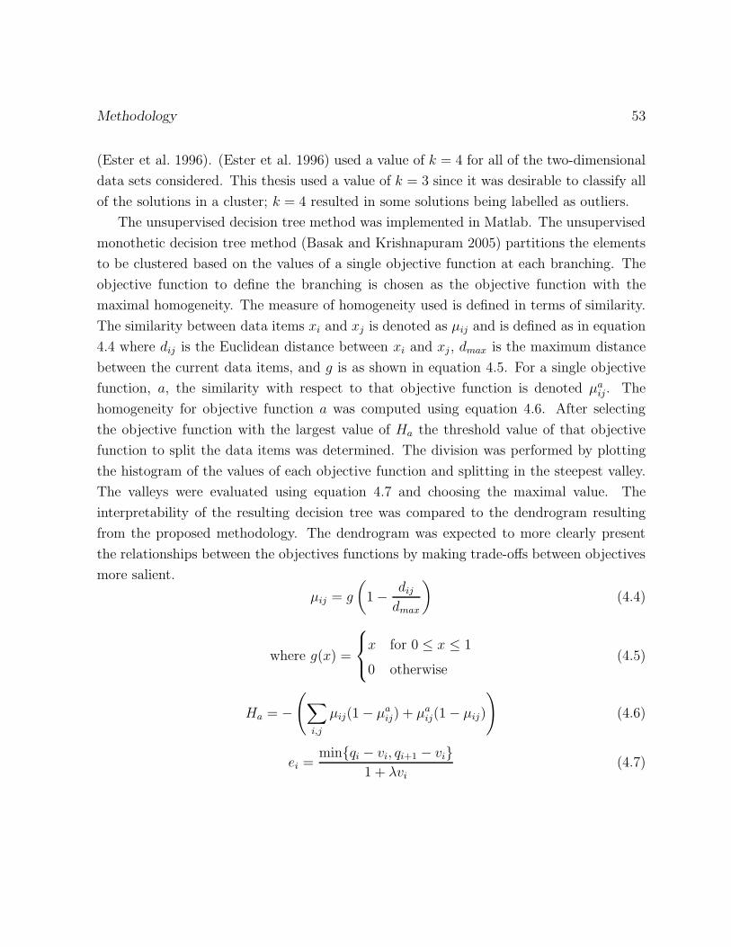
Methodology 53
(Ester et al. 1996). (Ester et al. 1996) used a value of k = 4 for all of the two-dimensional
data sets considered. This thesis used a value of k = 3 since it was desirable to classify all
of the solutions in a cluster; k = 4 resulted in some solutions being labelled as outliers.
The unsupervised decision tree method was implemented in Matlab. The unsupervised
monothetic decision tree method (Basak and Krishnapuram 2005) partitions the elements
to be clustered based on the values of a single objective function at each branching. The
objective function to define the branching is chosen as the objective function with the
maximal homogeneity. The measure of homogeneity used is defined in terms of similarity.
The similarity between data items xi and xj is denoted as µij and is defined as in equation
4.4 where dij is the Euclidean distance between xi and xj , dmax is the maximum distance
between the current data items, and g is as shown in equation 4.5. For a single objective
function, a, the similarity with respect to that objective function is denoted µaij. The
homogeneity for objective function a was computed using equation 4.6. After selecting
the objective function with the largest value of Ha the threshold value of that objective
function to split the data items was determined. The division was performed by plotting
the histogram of the values of each objective function and splitting in the steepest valley.
The valleys were evaluated using equation 4.7 and choosing the maximal value. The
interpretability of the resulting decision tree was compared to the dendrogram resulting
from the proposed methodology. The dendrogram was expected to more clearly present
the relationships between the objectives functions by making trade-offs between objectives
more salient.
µij = g
(
1− dij
dmax
)
(4.4)
where g(x) =
x for 0 ≤ x ≤ 1
0 otherwise(4.5)
Ha = −(
∑
i,j
µij(1− µaij) + µa
ij(1− µij)
)
(4.6)
ei =min{qi − vi, qi+1 − vi}
1 + λvi
(4.7)
54 Clustering Multiobjective Programming for Land Use Planning
4.3 Evaluation Methodology
After applying the cluster analysis methodology described in section 4.1.4 and the methods
for comparison, the results of these clustering methods, average linkage hierarchical clus-
tering described in section 4.1.5, Chameleon, DBSCAN, and the unsupervised decision tree
method described in section 4.2, were considered and evaluated. The proposed hierarchical
clustering method was considered based on cluster validity as described in section 4.1.6.
While it is not the focus of this thesis, the methodology and evaluation presented
employed visualization of the cluster hierarchy, individual clusters, and the relationships
between the objective functions. Clusters were visualized using a parallel axis plot (or value
path plot) as in Jankowski et al. (2001), matrices of scatter plots are used to visualize
objective function relationships, and dendrograms represent the cluster hierarchies. In
future work, these plots will be linked with maps to allow the decision makers to explore
the solution space as recommended by Jankowski et al. (2001).
The most important measure of success of the cluster analysis is the relevance and
correspondence with the application, in this case the land use configuration design prob-
lem. To assess this usefulness each branching in the hierarchy was considered to determine
whether the trade-off represented by choosing one of the resulting clusters over the other
cluster is reasonable. For illustrative purposes, and to consider the use of the structure in
a land use decision process, an example decision is presented in section 5.3. The example
decision begins with a case study decision context giving the decision makers concerns
and priorities and follows through the use of the hierarchical cluster tree until only a few
potential land use configurations remain under consideration. Since other aspects of the
decision may not have been modelled, the tree is not used to select a single solution for
implementation but rather a set of good solutions for further consideration. This exam-
ple decision and the consideration of the dendrogram branchings and the corresponding
landscape configurations encompass the external validity assessment.
The cophenetic correlation coefficient, perturbation testing, and subset clustering were
used to assess the internal validity of the structure resulting from the proposed method-
ology. The cophenetic correlation coefficient measures how closely the dendrogram tree
structure reflects the proximity matrix. In this thesis this measure relates to how well
the summary structure of the data used in the decision process reflects the trade-offs and
Methodology 55
relationships of the objective functions measuring the performance of the landscape con-
figuration. As well, the NSGA-II results were modified by adding random perturbation
factors to assess the stability of the dendrogram; the size of the perturbations required to
significantly change the upper levels of the dendrogram is determined as a measure of the
robustness of the cluster structure. As a third test of the internal validity, the NSGA-II
results were randomly split into two subsets and the resulting dendrograms were compared
to the initial dendrogram using all of the NSGA-II results.
To assess the relative validity the results of a second hierarchical clustering linkage
method were compared to the results of the proposed hierarchical clustering methodology.
If the underlying cluster models differ then agreement in the dendrogram structure indicates
true cluster structure in the data. The second hierarchical clustering linkage method
applied was the complete linkage method as discussed in section 4.1.4. The alternative
comparable methods listed in section 4.2 were also compared to the proposed methodology
to determine whether these methods provide a better summary structure of the data.
Chapter 5 reports the results of applying the methods presented in this chapter. Chap-
ter 6 discusses those results and chapter 7 gives conclusions and items for future work.

Chapter 5
Results
The methodology described in chapter 4 was applied to the 171 landscape configurations
in the NSGA-II results. This chapter details the results, following the outline in the last
chapter, beginning with establishing a clustering tendency and includes the application
of the hierarchical clustering method and cluster validation. Following the application of
the proposed methodology an example decision for the land use configuration problem is
outlined to demonstrate how the cluster analysis results can be used in decision-making. At
the end of this chapter the results of the comparable methods, Chameleon, DBSCAN, and
an unsupervised decision tree algorithm, are presented. Chapter 6 discusses the results
presented in this chapter and chapter 7 presents conclusions and recommendations for
future work.
5.1 Results of Cluster Analysis
This section includes the results of the cluster analysis as described in chapter 4. It
begins by establishing the existence of a hierarchical clustering tendency and discusses the
preparation for the cluster analysis. The results of applying the weighted group average
linkage hierarchical clustering algorithm are reported. Section 5.2 discusses the validity of
these results.
57
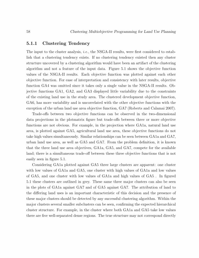
58 Clustering Multiobjective Programming for Land Use Planning
5.1.1 Clustering Tendency
The input to the cluster analysis, i.e., the NSGA-II results, were first considered to estab-
lish that a clustering tendency exists. If no clustering tendency existed then any cluster
structure uncovered by a clustering algorithm would have been an artifact of the clustering
algorithm and not a feature of the input data. Figure 5.1 shows the objective function
values of the NSGA-II results. Each objective function was plotted against each other
objective function. For ease of interpretation and consistency with later results, objective
function GA4 was omitted since it takes only a single value in the NSGA-II results. Ob-
jective functions GA1, GA2, and GA3 displayed little variability due to the constraints
of the existing land use in the study area. The clustered development objective function,
GA6, has more variability and is uncorrelated with the other objective functions with the
exception of the urban land use area objective function, GA7 (Roberts and Calamai 2007).
Trade-offs between two objective functions can be observed in the two-dimensional
data projections in the plotmatrix figure but trade-offs between three or more objective
functions are not obvious. For example, in the projection where GA1a, natural land use
area, is plotted against GA5, agricultural land use area, these objective functions do not
take high values simultaneously. Similar relationships can be seen between GA1a and GA7,
urban land use area, as well as GA5 and GA7. From the problem definition, it is known
that the three land use area objectives, GA1a, GA5, and GA7, compete for the available
land; there is a simultaneous trade-off between these three objective functions that is not
easily seen in figure 5.1.
Considering GA1a plotted against GA5 three large clusters are apparent: one cluster
with low values of GA1a and GA5, one cluster with high values of GA1a and low values
of GA5, and one cluster with low values of GA1a and high values of GA5 . In figured
5.1 these clusters are outlined in grey. These same three major clusters can also be seen
in the plots of GA1a against GA7 and of GA5 against GA7. The attribution of land to
the differing land uses is an important characteristic of this decision and the presence of
these major clusters should be detected by any successful clustering algorithm. Within the
major clusters several smaller subclusters can be seen, confirming the expected hierarchical
cluster structure. For example, in the cluster where both GA1a and GA5 take low values
there are five well-separated dense regions. The true structure may not correspond directly
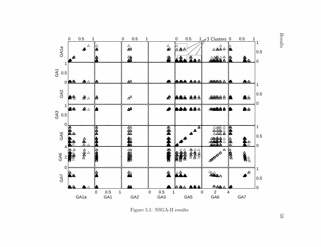
Resu
lts59
0
0.5
1
GA70 2 4
GA6
GA50 0.5 1
GA3
GA20 0.5 1
GA1
GA1a
GA
7
0
2
4
GA
6
0
0.5
1
GA
5
0
0.5
1
GA
3
0
0.5
1
GA
2
0
0.5
1
GA
1
0 0.5 1
0
0.5
10 0.5 10 0.5 10 0.5 1
GA
1a
3 Clusters
Figure 5.1: NSGA-II results
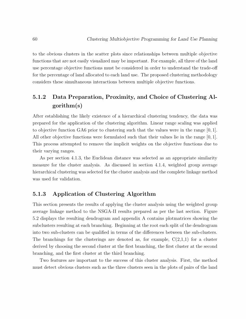
60 Clustering Multiobjective Programming for Land Use Planning
to the obvious clusters in the scatter plots since relationships between multiple objective
functions that are not easily visualized may be important. For example, all three of the land
use percentage objective functions must be considered in order to understand the trade-off
for the percentage of land allocated to each land use. The proposed clustering methodology
considers these simultaneous interactions between multiple objective functions.
5.1.2 Data Preparation, Proximity, and Choice of Clustering Al-
gorithm(s)
After establishing the likely existence of a hierarchical clustering tendency, the data was
prepared for the application of the clustering algorithm. Linear range scaling was applied
to objective function GA6 prior to clustering such that the values were in the range [0, 1].
All other objective functions were formulated such that their values lie in the range [0, 1].
This process attempted to remove the implicit weights on the objective functions due to
their varying ranges.
As per section 4.1.3, the Euclidean distance was selected as an appropriate similarity
measure for the cluster analysis. As discussed in section 4.1.4, weighted group average
hierarchical clustering was selected for the cluster analysis and the complete linkage method
was used for validation.
5.1.3 Application of Clustering Algorithm
This section presents the results of applying the cluster analysis using the weighted group
average linkage method to the NSGA-II results prepared as per the last section. Figure
5.2 displays the resulting dendrogram and appendix A contains plotmatrices showing the
subclusters resulting at each branching. Beginning at the root each split of the dendrogram
into two sub-clusters can be qualified in terms of the differences between the sub-clusters.
The branchings for the clusterings are denoted as, for example, C(2,1,1) for a cluster
derived by choosing the second cluster at the first branching, the first cluster at the second
branching, and the first cluster at the third branching.
Two features are important to the success of this cluster analysis. First, the method
must detect obvious clusters such as the three clusters seen in the plots of pairs of the land
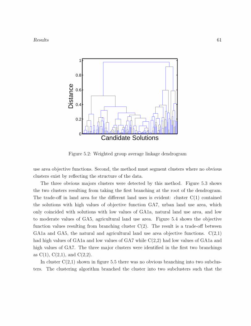
Results 61
0
0.2
0.4
0.6
0.8
1
Candidate Solutions
Dis
tanc
e
Figure 5.2: Weighted group average linkage dendrogram
use area objective functions. Second, the method must segment clusters where no obvious
clusters exist by reflecting the structure of the data.
The three obvious majors clusters were detected by this method. Figure 5.3 shows
the two clusters resulting from taking the first branching at the root of the dendrogram.
The trade-off in land area for the different land uses is evident: cluster C(1) contained
the solutions with high values of objective function GA7, urban land use area, which
only coincided with solutions with low values of GA1a, natural land use area, and low
to moderate values of GA5, agricultural land use area. Figure 5.4 shows the objective
function values resulting from branching cluster C(2). The result is a trade-off between
GA1a and GA5, the natural and agricultural land use area objective functions. C(2,1)
had high values of GA1a and low values of GA7 while C(2,2) had low values of GA1a and
high values of GA7. The three major clusters were identified in the first two branchings
as C(1), C(2,1), and C(2,2).
In cluster C(2,1) shown in figure 5.5 there was no obvious branching into two subclus-
ters. The clustering algorithm branched the cluster into two subclusters such that the
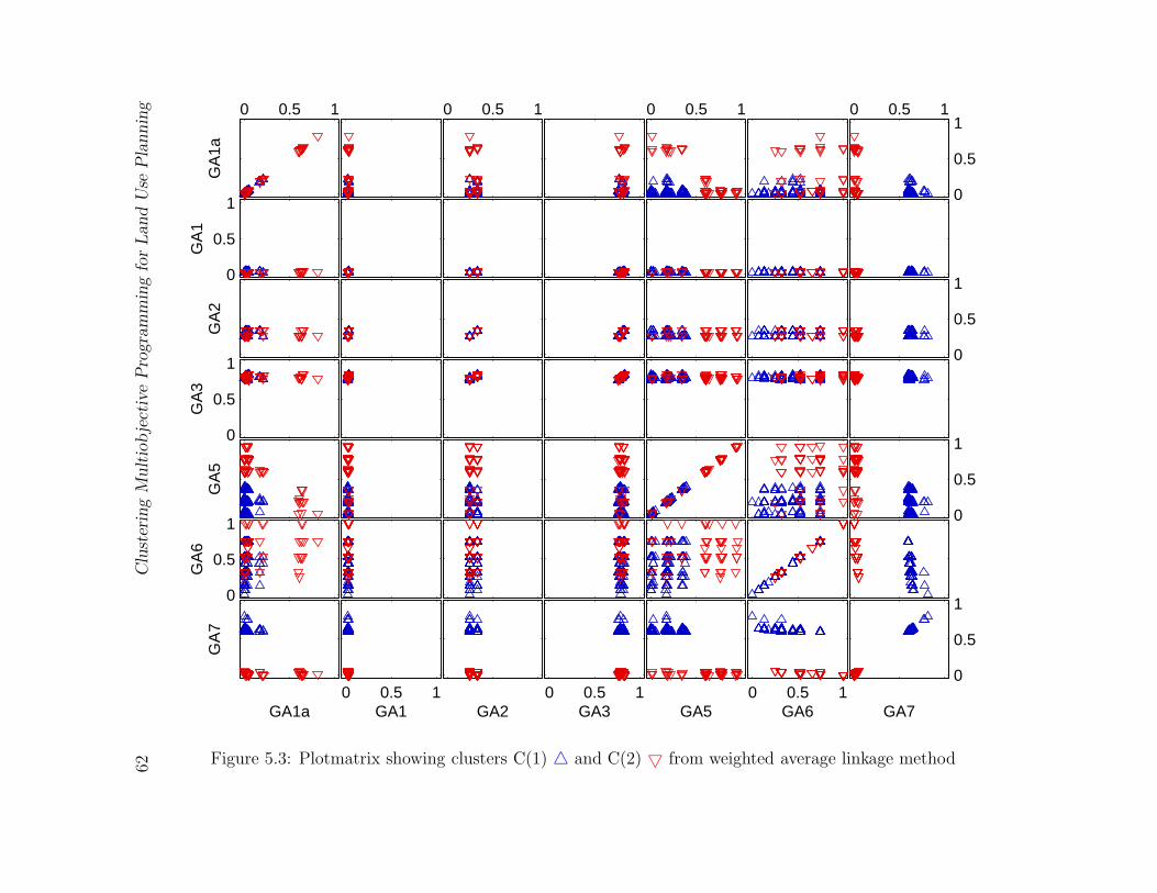
62C
lust
erin
gM
ult
iobje
ctiv
eP
rogra
mm
ing
for
Land
Use
Pla
nnin
g
0
0.5
1
GA70 0.5 1
GA6
GA50 0.5 1
GA3
GA20 0.5 1
GA1
GA1a
GA
7
0
0.5
1
GA
6
0
0.5
1
GA
5
0
0.5
1
GA
3
0
0.5
1
GA
2
0
0.5
1G
A1
0 0.5 1
0
0.5
10 0.5 10 0.5 10 0.5 1
GA
1a
Figure 5.3: Plotmatrix showing clusters C(1) 4 and C(2) 5 from weighted average linkage method
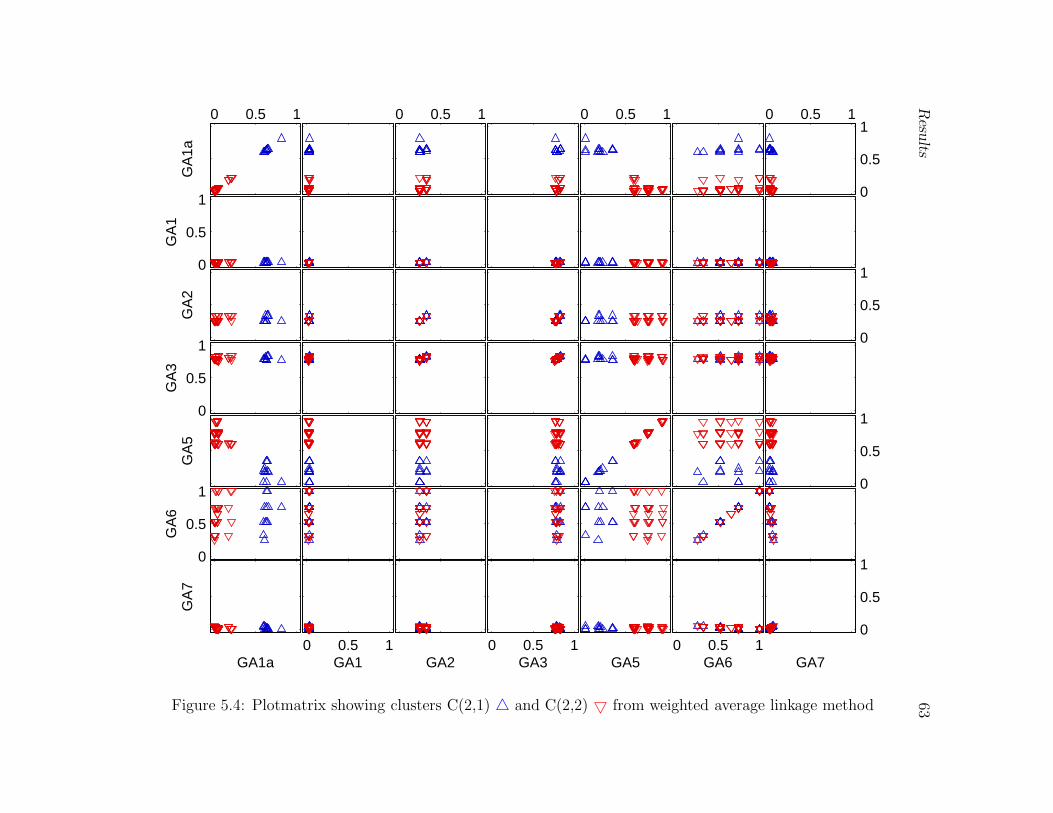
Resu
lts63
0
0.5
1
GA70 0.5 1
GA6
GA50 0.5 1
GA3
GA20 0.5 1
GA1
GA1a
GA
7
0
0.5
1
GA
6
0
0.5
1
GA
5
0
0.5
1
GA
3
0
0.5
1
GA
2
0
0.5
1
GA
1
0 0.5 1
0
0.5
10 0.5 10 0.5 10 0.5 1
GA
1a
Figure 5.4: Plotmatrix showing clusters C(2,1) 4 and C(2,2) 5 from weighted average linkage method
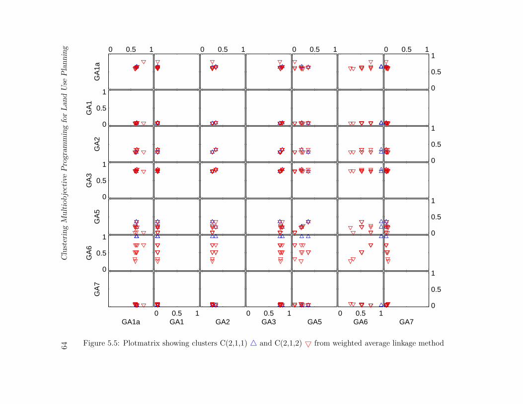
64C
lust
erin
gM
ult
iobje
ctiv
eP
rogra
mm
ing
for
Land
Use
Pla
nnin
g
0
0.5
1
GA70 0.5 1
GA6
GA50 0.5 1
GA3
GA20 0.5 1
GA1
GA1a
GA
7
0
0.5
1
GA
6
0
0.5
1
GA
5
0
0.5
1
GA
3
0
0.5
1
GA
2
0
0.5
1G
A1
0 0.5 1
0
0.5
10 0.5 10 0.5 10 0.5 1
GA
1a
Figure 5.5: Plotmatrix showing clusters C(2,1,1) 4 and C(2,1,2) 5 from weighted average linkage method
Results 65
solutions in cluster C(2,1,1) were preferable to those in cluster C(2,1,2) on objective func-
tion GA6, clustered development on which they all attained the maximal value. As well,
no solution in cluster C(2,1,1) took the minimal value for objective function GA5, agricul-
tural land use area. The solutions in cluster C(2,1,2) attained similar or better values of
objective function GA1a, natural land use area, than the solutions in cluster C(2,1,1) and
similar or worse values of objective function GA5, agricultural land use area. None of the
solutions in cluster C(2,1,2) took a value of zero for objective function GA7, urban land
use area, and no solution in cluster C(2,1,1) included any new urban land use area. These
subclusters were clearly different and reflected trade-offs between the objective functions.
After using the clustering structure to select one or more clusters at this level as poten-
tial solutions, other elements of the decision that were not modelled should be considered,
such as political issues or costs of obtaining or transforming certain land parcels. The
following section presents the results of cluster validation for these results. Section 5.3 de-
scribes a hypothetical decision scenario and demonstrates how the structure and trade-off
information returned by the clustering methodology can be used to aid in the selection of
good land use configurations for further investigation. At the end of the decision process
using the clustering structure, the land use codings for the selected candidate sites are
considered.
5.2 Validation of Cluster Analysis Results
This section presents the results of three types of validation for the cluster analysis. Inter-
nal, external, and relative validity, as described in section 4.1.6, are considered.
5.2.1 Internal Validity
The cophenetic correlation coefficient, as described in section 4.1.6, was 0.9247 for the
weighted group average linkage method and 0.9124 for the complete linkage method. Both
of these values were sufficiently high to indicate that the dendrograms are good fits to the
data but the higher value for the weighted group average linkage method cannot be used
as an indicator of a better fit since the cophenetic correlation coefficient value depends on
the linkage method.
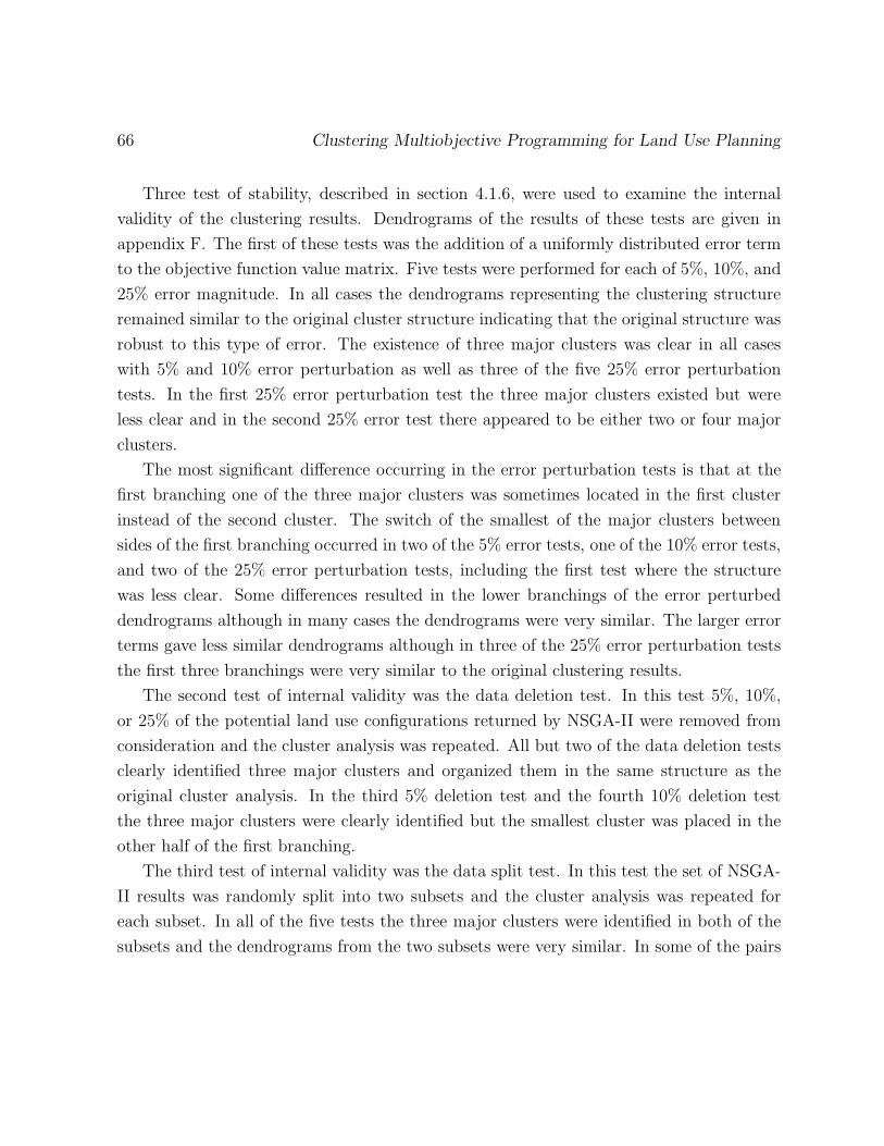
66 Clustering Multiobjective Programming for Land Use Planning
Three test of stability, described in section 4.1.6, were used to examine the internal
validity of the clustering results. Dendrograms of the results of these tests are given in
appendix F. The first of these tests was the addition of a uniformly distributed error term
to the objective function value matrix. Five tests were performed for each of 5%, 10%, and
25% error magnitude. In all cases the dendrograms representing the clustering structure
remained similar to the original cluster structure indicating that the original structure was
robust to this type of error. The existence of three major clusters was clear in all cases
with 5% and 10% error perturbation as well as three of the five 25% error perturbation
tests. In the first 25% error perturbation test the three major clusters existed but were
less clear and in the second 25% error test there appeared to be either two or four major
clusters.
The most significant difference occurring in the error perturbation tests is that at the
first branching one of the three major clusters was sometimes located in the first cluster
instead of the second cluster. The switch of the smallest of the major clusters between
sides of the first branching occurred in two of the 5% error tests, one of the 10% error tests,
and two of the 25% error perturbation tests, including the first test where the structure
was less clear. Some differences resulted in the lower branchings of the error perturbed
dendrograms although in many cases the dendrograms were very similar. The larger error
terms gave less similar dendrograms although in three of the 25% error perturbation tests
the first three branchings were very similar to the original clustering results.
The second test of internal validity was the data deletion test. In this test 5%, 10%,
or 25% of the potential land use configurations returned by NSGA-II were removed from
consideration and the cluster analysis was repeated. All but two of the data deletion tests
clearly identified three major clusters and organized them in the same structure as the
original cluster analysis. In the third 5% deletion test and the fourth 10% deletion test
the three major clusters were clearly identified but the smallest cluster was placed in the
other half of the first branching.
The third test of internal validity was the data split test. In this test the set of NSGA-
II results was randomly split into two subsets and the cluster analysis was repeated for
each subset. In all of the five tests the three major clusters were identified in both of the
subsets and the dendrograms from the two subsets were very similar. In some of the pairs
Results 67
of subsets some of the branching heights differed between the two subsets. In the first
half of the second test one of the major clusters was placed on the other side of the first
branching.
The switching of a major cluster between the two halves, in all three types of validity
tests, indicated that the order of the first two branchings is not robust to error in the
data. The dendrograms represent this element of the cluster structure by the heights of
the branchings representing the inconsistency measures for branchings. Branchings that
occur at approximately the same height have small inconsistency values. Highly differ-
entiating branchings exist where a significant height difference exists between successive
branchings. While this feature of the dendrogram does reflect the similar importance of
the first branching and the second branching of the cluster containing two of the major
clusters, a three-way branching in a tree may be more interpretable (e.g., cf. the structure
for DBSCAN in figure 5.21).
In most of the tests some of the structure of the lower clusters remained similar to
the original clustering results although the clustering structures were only highly similar
to two branchings. This variation may be due to less clear clustering in the lower, and
therefore smaller, clusters since fewer elements existed to define the clusters. As well, the
hierarchical cluster structure was a more accurate representation at the higher levels of the
dendrogram.
In summary, based on the value cophenetic correlation coefficient and the stability tests,
the internal validity, of the weighted group average linkage method results was satisfactory.
The cophenetic correlation coefficient was sufficiently large to indicate a good fit of the
dendrogram to the data. All three types of stability tests: error perturbation, data deletion,
and data split, indicated that the three major clusters that were detected are a valid
structure. Which of the three major clusters are defined at the first and second branchings
was less definite but that was reflected in the similar heights in the original dendrogram.
The clusters due to branchings resulting lower in the dendrogram were less robust than
the clusters from branchings higher in the dendrogram. This reduced robustness reflected
that those clusters are less differentiated and in many cases they were not the result of an
obvious cluster structure.
68 Clustering Multiobjective Programming for Land Use Planning
5.2.2 External Validity
The objective functions measure the performance of the landscape configuration. The set
of landscape configurations in each cluster was considered to determine whether the group-
ing of those configurations was reasonable and whether it corresponded to the objective
function values as expected. This consideration of the landscape configurations is similar
to consulting a subject matter expert in order to validate the cluster analysis in terms of
the real world aspects of the decision. The site codings occurring in the clusters are shown
in figures A.8 through A.14 in appendix A. The candidate site numbers correspond to
the map shown in figure 3.1. The objective functions were formulated in order to favour
landscape designs with large connected natural areas as well as compact natural core areas
(Roberts and Calamai 2007). As a verification of external validity, the resulting clusters
should correspond to differing sets of landscape designs with these characteristics.
Objective functions GA1a, GA5, and GA7 compute the additional natural, agricultural,
and urban area, respectively, resulting from the allocation of the candidate sites to each
of these land use categories. These land area objective functions should compete for the
larger sites. Site 4 is the largest candidate site. Sites 1 and 5 are large and sites 3, 7,
and 8 are small. In the NSGA-II results most of the candidate sites took every land use
code at least once; the exceptions are that site three is never agricultural, site four is never
unchanged, and site five is never urban.
Roberts and Calamai (2007) considered the same landscape configuration design prob-
lem for the same study area without eliminating small ‘sliver’ polygons. Objective function
GA2 measures the connectivity of the natural areas. Roberts and Calamai (2007) noted
that the two large existing natural areas cannot be connected by coding candidate sites
as natural. That limitation of the landscape remained true when the sliver polygons were
removed. Roberts and Calamai (2007) also noted that coding the candidate sites num-
bered one and two in this thesis as natural allows a small two polygon natural area to
be connected to the largest natural area. The largest natural area is increased in area by
coding any of the candidate sites three, four, five, seven, and eight as natural. Coding
candidate site six as natural increases the area of the second natural core area. As in
Roberts and Calamai (2007), one natural polygon located in the upper centre of the study
area could not be joined to any of the other natural areas. There are no candidate sites
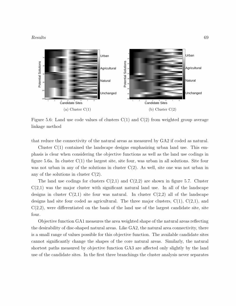
Results 69
Candidate Sites
Pot
entia
l Sol
utio
ns
1 2 3 4 5 6 7 8
20
40
60
80
100
120
Unchanged
Natural
Agricultural
Urban
(a) Cluster C(1)
Candidate Sites
Pot
entia
l Sol
utio
ns
1 2 3 4 5 6 7 8
5
10
15
20
25
30
35
40
45
50
Unchanged
Natural
Agricultural
Urban
(b) Cluster C(2)
Figure 5.6: Land use code values of clusters C(1) and C(2) from weighted group average
linkage method
that reduce the connectivity of the natural areas as measured by GA2 if coded as natural.
Cluster C(1) contained the landscape designs emphasizing urban land use. This em-
phasis is clear when considering the objective functions as well as the land use codings in
figure 5.6a. In cluster C(1) the largest site, site four, was urban in all solutions. Site four
was not urban in any of the solutions in cluster C(2). As well, site one was not urban in
any of the solutions in cluster C(2).
The land use codings for clusters C(2,1) and C(2,2) are shown in figure 5.7. Cluster
C(2,1) was the major cluster with significant natural land use. In all of the landscape
designs in cluster C(2,1) site four was natural. In cluster C(2,2) all of the landscape
designs had site four coded as agricultural. The three major clusters, C(1), C(2,1), and
C(2,2), were differentiated on the basis of the land use of the largest candidate site, site
four.
Objective function GA1 measures the area weighted shape of the natural areas reflecting
the desirability of disc-shaped natural areas. Like GA2, the natural area connectivity, there
is a small range of values possible for this objective function. The available candidate sites
cannot significantly change the shapes of the core natural areas. Similarly, the natural
shortest paths measured by objective function GA3 are affected only slightly by the land
use of the candidate sites. In the first three branchings the cluster analysis never separates
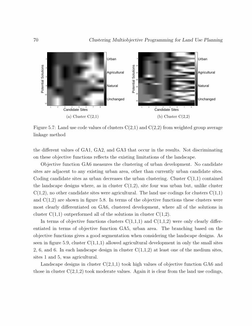
70 Clustering Multiobjective Programming for Land Use Planning
Candidate Sites
Pot
entia
l Sol
utio
ns
1 2 3 4 5 6 7 8
2
4
6
8
10
12
Unchanged
Natural
Agricultural
Urban
(a) Cluster C(2,1)
Candidate Sites
Pot
entia
l Sol
utio
ns
1 2 3 4 5 6 7 8
5
10
15
20
25
30
35Unchanged
Natural
Agricultural
Urban
(b) Cluster C(2,2)
Figure 5.7: Land use code values of clusters C(2,1) and C(2,2) from weighted group average
linkage method
the different values of GA1, GA2, and GA3 that occur in the results. Not discriminating
on these objective functions reflects the existing limitations of the landscape.
Objective function GA6 measures the clustering of urban development. No candidate
sites are adjacent to any existing urban area, other than currently urban candidate sites.
Coding candidate sites as urban decreases the urban clustering. Cluster C(1,1) contained
the landscape designs where, as in cluster C(1,2), site four was urban but, unlike cluster
C(1,2), no other candidate sites were agricultural. The land use codings for clusters C(1,1)
and C(1,2) are shown in figure 5.8. In terms of the objective functions these clusters were
most clearly differentiated on GA6, clustered development, where all of the solutions in
cluster C(1,1) outperformed all of the solutions in cluster C(1,2).
In terms of objective functions clusters C(1,1,1) and C(1,1,2) were only clearly differ-
entiated in terms of objective function GA5, urban area. The branching based on the
objective functions gives a good segmentation when considering the landscape designs. As
seen in figure 5.9, cluster C(1,1,1) allowed agricultural development in only the small sites
2, 6, and 6. In each landscape design in cluster C(1,1,2) at least one of the medium sites,
sites 1 and 5, was agricultural.
Landscape designs in cluster C(2,1,1) took high values of objective function GA6 and
those in cluster C(2,1,2) took moderate values. Again it is clear from the land use codings,
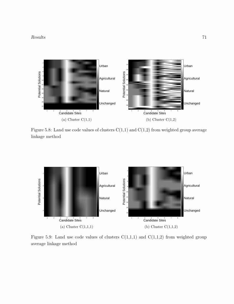
Results 71
Candidate Sites
Pot
entia
l Sol
utio
ns
1 2 3 4 5 6 7 8
2
4
6
8
10
12
14
16
18
20
22
Unchanged
Natural
Agricultural
Urban
(a) Cluster C(1,1)
Candidate Sites
Pot
entia
l Sol
utio
ns
1 2 3 4 5 6 7 8
10
20
30
40
50
60
70
80
90Unchanged
Natural
Agricultural
Urban
(b) Cluster C(1,2)
Figure 5.8: Land use code values of clusters C(1,1) and C(1,2) from weighted group average
linkage method
Candidate Sites
Pot
entia
l Sol
utio
ns
1 2 3 4 5 6 7 8
1
2
3
4 Unchanged
Natural
Agricultural
Urban
(a) Cluster C(1,1,1)
Candidate Sites
Pot
entia
l Sol
utio
ns
1 2 3 4 5 6 7 8
2
4
6
8
10
12
14
16
18Unchanged
Natural
Agricultural
Urban
(b) Cluster C(1,1,2)
Figure 5.9: Land use code values of clusters C(1,1,1) and C(1,1,2) from weighted group
average linkage method
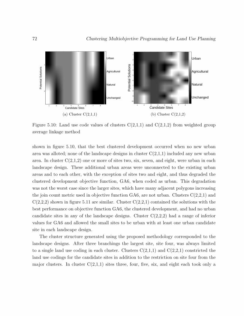
72 Clustering Multiobjective Programming for Land Use Planning
Candidate Sites
Pot
entia
l Sol
utio
ns
1 2 3 4 5 6 7 8
1
2
Unchanged
Natural
Agricultural
Urban
(a) Cluster C(2,1,1)
Candidate Sites
Pot
entia
l Sol
utio
ns
1 2 3 4 5 6 7 8
1
2
3
4
5
6
7
8
9
10
Unchanged
Natural
Agricultural
Urban
(b) Cluster C(2,1,2)
Figure 5.10: Land use code values of clusters C(2,1,1) and C(2,1,2) from weighted group
average linkage method
shown in figure 5.10, that the best clustered development occurred when no new urban
area was alloted; none of the landscape designs in cluster C(2,1,1) included any new urban
area. In cluster C(2,1,2) one or more of sites two, six, seven, and eight, were urban in each
landscape design. These additional urban areas were unconnected to the existing urban
areas and to each other, with the exception of sites two and eight, and thus degraded the
clustered development objective function, GA6, when coded as urban. This degradation
was not the worst case since the larger sites, which have many adjacent polygons increasing
the join count metric used in objective function GA6, are not urban. Clusters C(2,2,1) and
C(2,2,2) shown in figure 5.11 are similar. Cluster C(2,2,1) contained the solutions with the
best performance on objective function GA6, the clustered development, and had no urban
candidate sites in any of the landscape designs. Cluster C(2,2,2) had a range of inferior
values for GA6 and allowed the small sites to be urban with at least one urban candidate
site in each landscape design.
The cluster structure generated using the proposed methodology corresponded to the
landscape designs. After three branchings the largest site, site four, was always limited
to a single land use coding in each cluster. Clusters C(2,1,1) and C(2,2,1) constricted the
land use codings for the candidate sites in addition to the restriction on site four from the
major clusters. In cluster C(2,1,1) sites three, four, five, six, and eight each took only a
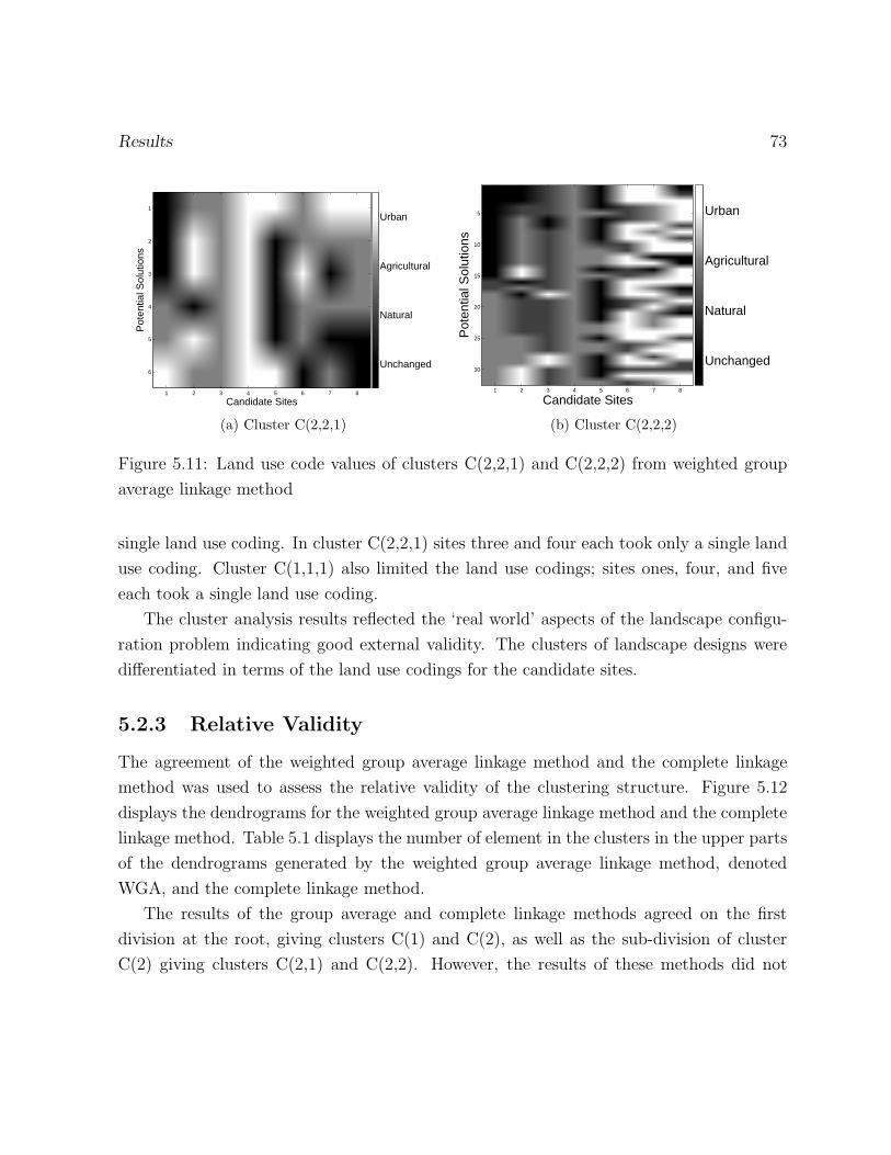
Results 73
Candidate Sites
Pot
entia
l Sol
utio
ns
1 2 3 4 5 6 7 8
1
2
3
4
5
6Unchanged
Natural
Agricultural
Urban
(a) Cluster C(2,2,1)
Candidate Sites
Pot
entia
l Sol
utio
ns
1 2 3 4 5 6 7 8
5
10
15
20
25
30Unchanged
Natural
Agricultural
Urban
(b) Cluster C(2,2,2)
Figure 5.11: Land use code values of clusters C(2,2,1) and C(2,2,2) from weighted group
average linkage method
single land use coding. In cluster C(2,2,1) sites three and four each took only a single land
use coding. Cluster C(1,1,1) also limited the land use codings; sites ones, four, and five
each took a single land use coding.
The cluster analysis results reflected the ‘real world’ aspects of the landscape configu-
ration problem indicating good external validity. The clusters of landscape designs were
differentiated in terms of the land use codings for the candidate sites.
5.2.3 Relative Validity
The agreement of the weighted group average linkage method and the complete linkage
method was used to assess the relative validity of the clustering structure. Figure 5.12
displays the dendrograms for the weighted group average linkage method and the complete
linkage method. Table 5.1 displays the number of element in the clusters in the upper parts
of the dendrograms generated by the weighted group average linkage method, denoted
WGA, and the complete linkage method.
The results of the group average and complete linkage methods agreed on the first
division at the root, giving clusters C(1) and C(2), as well as the sub-division of cluster
C(2) giving clusters C(2,1) and C(2,2). However, the results of these methods did not
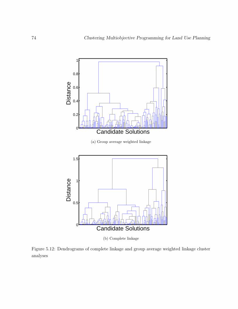
74 Clustering Multiobjective Programming for Land Use Planning
0
0.2
0.4
0.6
0.8
1
Candidate Solutions
Dis
tanc
e
(a) Group average weighted linkage
0
0.5
1
1.5
Candidate Solutions
Dis
tanc
e
(b) Complete linkage
Figure 5.12: Dendrograms of complete linkage and group average weighted linkage cluster
analyses
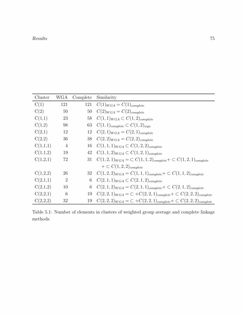
Results 75
Cluster WGA Complete Similarity
C(1) 121 121 C(1)WGA = C(1)complete
C(2) 50 50 C(2)WGA = C(2)complete
C(1,1) 23 58 C(1, 1)WGA ⊂ C(1, 2)complete
C(1,2) 98 63 C(1, 1)complete ⊂ C(1, 2)wga
C(2,1) 12 12 C(2, 1)WGA = C(2, 1)complete
C(2,2) 36 38 C(2, 2)WGA = C(2, 2)complete
C(1,1,1) 4 16 C(1, 1, 1)WGA ⊂ C(1, 2, 2)complete
C(1,1,2) 19 42 C(1, 1, 2)WGA ⊂ C(1, 2, 1)complete
C(1,2,1) 72 31 C(1, 2, 1)WGA =⊂ C(1, 1, 2)complete+ ⊂ C(1, 2, 1)complete
+ ⊂ C(1, 2, 2)complete
C(1,2,2) 26 32 C(1, 2, 2)WGA = C(1, 1, 1)complete+ ⊂ C(1, 1, 2)complete
C(2,1,1) 2 6 C(2, 1, 1)WGA ⊂ C(2, 1, 2)complete
C(2,1,2) 10 6 C(2, 1, 2)WGA = C(2, 1, 1)complete+ ⊂ C(2, 1, 2)complete
C(2,2,1) 6 19 C(2, 2, 1)WGA =⊂ +C(2, 2, 1)complete+ ⊂ C(2, 2, 2)complete
C(2,2,2) 32 19 C(2, 2, 2)WGA =⊂ +C(2, 2, 1)complete+ ⊂ C(2, 2, 2)complete
Table 5.1: Number of elements in clusters of weighted group average and complete linkage
methods
76 Clustering Multiobjective Programming for Land Use Planning
agree at the division of cluster C(1) giving clusters C(1,1) and C(1,2) and at each division
following from that branching. The weighted group average linkage method split cluster
C(1) into two well separated groups that differed in their values of objective function GA6,
clustered development. The complete linkage method gave a more balanced branching
at a narrower separation in the values of objective function GA6. The weighted group
average linkage method placed all of the solutions with higher values of GA1a, natural
land area, in cluster C(1,2), along with some solutions with lower values of GA1a, while
the complete linkage method placed some of these solutions in each cluster. This splitting
by the weighted group average linkage method resulted in cluster C(1,1) having a very
little variability in objective function GA1a while both of the subclusters of C(1) in the
complete linkage method had a range that is similar to C(1).
The complete linkage method may force the clusters to be balanced even if the un-
derlying structure does not include balanced clusters. The group average method makes
no such assumption. At a branching, the assumption of balanced clusters should lead
to two subclusters containing approximately the same number of solutions. The number
of solutions in each cluster for the weighted group average and complete linkage meth-
ods is given in table 5.1. For example, the two clusters, C(1,1) and C(1,2), that result
from branching cluster C(1), are unbalanced in the weighted group average method re-
sults; cluster C(1,1) contains 23 solutions while cluster C(1,2) contains 98 solutions. In
contrast, these same clusters in the complete linkage results are balanced; cluster C(1,1)
contains 58 solutions while cluster C(1,2) contains 63 solutions. Similar behaviour is seen
when branching C(1,2), C(2,1), and C(2,2). Since this behaviour of the complete linkage
method corresponds to a known assumption of that method, it is likely that the actual
structure contains unbalanced clusters. Considering these same clusters in the complete
linkage method results, the complete linkage method segmented the larger cluster found
by the group average method and thus occluded the smaller cluster. The balanced clusters
in the complete linkage method, relative to the weighted group average linkage method,
can be seen in figure 5.12.
The weighted group average linkage method results tended to agree with the complete
linkage method indicating good relative validity. The discrepancies in the results from
these methods can be attributed to known assumptions of the complete linkage method;
Results 77
the weighted group average results were more valid where these discrepancies existed.
The internal, external, and relative validity assessments of the weighted group average
method results indicated that these results are a good representation of the input data and
the problem being modelled. These assessments confirmed that there were three major
clusters in the data and that the general dendrogram structure was valid although the
clusters lower in the dendrogram were less robust.
5.3 Example Decision Process
This section gives an example of the use of the hierarchical clustering structure developed
in this thesis in the land use decision described in section 3. The hypothetical decision
scenario reflects the emphasis on the objective functions. The local human population
requires land to work, live, and grow food, i.e., urban and agricultural land. Land at
the fringes of the currently developed areas is desirable for these purposes but this land
currently serves natural functions. For example, water recharge area and animal habitats
may exist within the natural area. In this thesis and previous work (Roberts 2003) the
natural functions that require specific land parcels, such as water recharge, were dealt
with by pre-processing and the natural functions that may not be specific to particular
land parcels, such as animal habitats, are dealt with using the multiobjective optimization
model for the landscape configuration problem. In this scenario there are several current
candidate sites whose land use can be changed. There is pressure for new land for urban
and agricultural uses as well as pressure to allocate some of the available land to the
natural systems in order to preserve the existing function of the landscape. None of the
stakeholders advocating each of the three types of land use is willing to accept that there
be no new area of that type. As is reflected by the number of related objective functions,
the most significant concern of the decision makers is the loss of natural land. New natural
land is most important in this area. The potential loss of natural land functions is related
to the first four objective functions and GA6 which measures the clustering of urban
development. The clustering of urban development is also desirable for human use of the
land, for example, services such as public transit and waste collection can be implemented
more efficiently in compact urban areas.
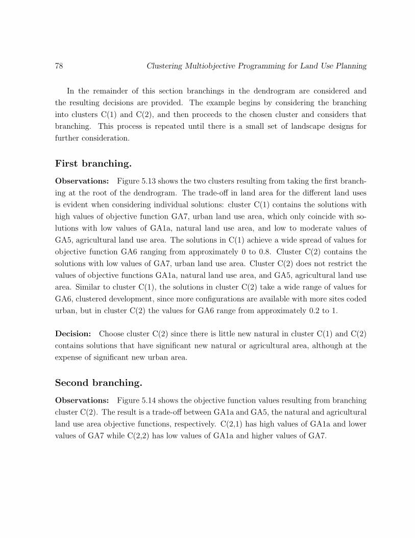
78 Clustering Multiobjective Programming for Land Use Planning
In the remainder of this section branchings in the dendrogram are considered and
the resulting decisions are provided. The example begins by considering the branching
into clusters C(1) and C(2), and then proceeds to the chosen cluster and considers that
branching. This process is repeated until there is a small set of landscape designs for
further consideration.
First branching.
Observations: Figure 5.13 shows the two clusters resulting from taking the first branch-
ing at the root of the dendrogram. The trade-off in land area for the different land uses
is evident when considering individual solutions: cluster C(1) contains the solutions with
high values of objective function GA7, urban land use area, which only coincide with so-
lutions with low values of GA1a, natural land use area, and low to moderate values of
GA5, agricultural land use area. The solutions in C(1) achieve a wide spread of values for
objective function GA6 ranging from approximately 0 to 0.8. Cluster C(2) contains the
solutions with low values of GA7, urban land use area. Cluster C(2) does not restrict the
values of objective functions GA1a, natural land use area, and GA5, agricultural land use
area. Similar to cluster C(1), the solutions in cluster C(2) take a wide range of values for
GA6, clustered development, since more configurations are available with more sites coded
urban, but in cluster C(2) the values for GA6 range from approximately 0.2 to 1.
Decision: Choose cluster C(2) since there is little new natural in cluster C(1) and C(2)
contains solutions that have significant new natural or agricultural area, although at the
expense of significant new urban area.
Second branching.
Observations: Figure 5.14 shows the objective function values resulting from branching
cluster C(2). The result is a trade-off between GA1a and GA5, the natural and agricultural
land use area objective functions, respectively. C(2,1) has high values of GA1a and lower
values of GA7 while C(2,2) has low values of GA1a and higher values of GA7.
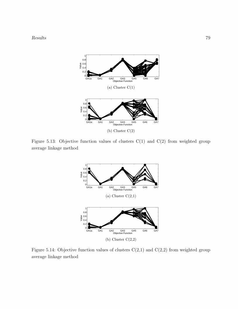
Results 79
GA1a GA1 GA2 GA3 GA5 GA6 GA70
0.2
0.4
0.6
0.8
1
Val
ueObjective Function
(a) Cluster C(1)
GA1a GA1 GA2 GA3 GA5 GA6 GA70
0.2
0.4
0.6
0.8
1
Val
ue
Objective Function
(b) Cluster C(2)
Figure 5.13: Objective function values of clusters C(1) and C(2) from weighted group
average linkage method
GA1a GA1 GA2 GA3 GA5 GA6 GA70
0.2
0.4
0.6
0.8
1
Val
ue
Objective Function
(a) Cluster C(2,1)
GA1a GA1 GA2 GA3 GA5 GA6 GA70
0.2
0.4
0.6
0.8
1
Val
ue
Objective Function
(b) Cluster C(2,2)
Figure 5.14: Objective function values of clusters C(2,1) and C(2,2) from weighted group
average linkage method
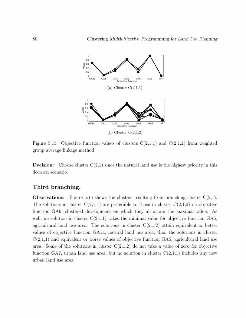
80 Clustering Multiobjective Programming for Land Use Planning
GA1a GA1 GA2 GA3 GA5 GA6 GA70
0.2
0.4
0.6
0.8
1
Val
ueObjective Function
(a) Cluster C(2,1,1)
GA1a GA1 GA2 GA3 GA5 GA6 GA70
0.2
0.4
0.6
0.8
1
Val
ue
Objective Function
(b) Cluster C(2,1,2)
Figure 5.15: Objective function values of clusters C(2,1,1) and C(2,1,2) from weighted
group average linkage method
Decision: Choose cluster C(2,1) since the natural land use is the highest priority in this
decision scenario.
Third branching.
Observations: Figure 5.15 shows the clusters resulting from branching cluster C(2,1).
The solutions in cluster C(2,1,1) are preferable to those in cluster C(2,1,2) on objective
function GA6, clustered development on which they all attain the maximal value. As
well, no solution in cluster C(2,1,1) takes the minimal value for objective function GA5,
agricultural land use area. The solutions in cluster C(2,1,2) attain equivalent or better
values of objective function GA1a, natural land use area, than the solutions in cluster
C(2,1,1) and equivalent or worse values of objective function GA5, agricultural land use
area. Some of the solutions in cluster C(2,1,2) do not take a value of zero for objective
function GA7, urban land use area, but no solution in cluster C(2,1,1) includes any new
urban land use area.
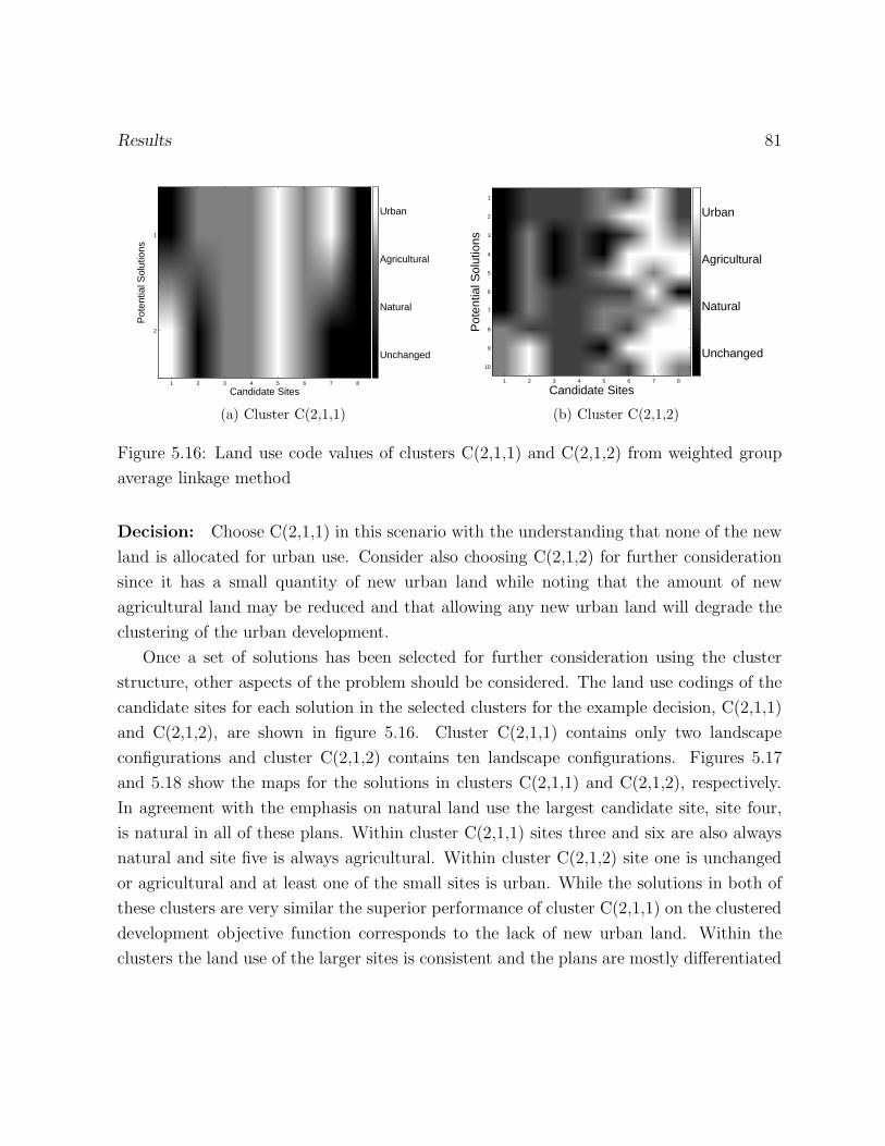
Results 81
Candidate Sites
Pot
entia
l Sol
utio
ns
1 2 3 4 5 6 7 8
1
2
Unchanged
Natural
Agricultural
Urban
(a) Cluster C(2,1,1)
Candidate Sites
Pot
entia
l Sol
utio
ns
1 2 3 4 5 6 7 8
1
2
3
4
5
6
7
8
9
10
Unchanged
Natural
Agricultural
Urban
(b) Cluster C(2,1,2)
Figure 5.16: Land use code values of clusters C(2,1,1) and C(2,1,2) from weighted group
average linkage method
Decision: Choose C(2,1,1) in this scenario with the understanding that none of the new
land is allocated for urban use. Consider also choosing C(2,1,2) for further consideration
since it has a small quantity of new urban land while noting that the amount of new
agricultural land may be reduced and that allowing any new urban land will degrade the
clustering of the urban development.
Once a set of solutions has been selected for further consideration using the cluster
structure, other aspects of the problem should be considered. The land use codings of the
candidate sites for each solution in the selected clusters for the example decision, C(2,1,1)
and C(2,1,2), are shown in figure 5.16. Cluster C(2,1,1) contains only two landscape
configurations and cluster C(2,1,2) contains ten landscape configurations. Figures 5.17
and 5.18 show the maps for the solutions in clusters C(2,1,1) and C(2,1,2), respectively.
In agreement with the emphasis on natural land use the largest candidate site, site four,
is natural in all of these plans. Within cluster C(2,1,1) sites three and six are also always
natural and site five is always agricultural. Within cluster C(2,1,2) site one is unchanged
or agricultural and at least one of the small sites is urban. While the solutions in both of
these clusters are very similar the superior performance of cluster C(2,1,1) on the clustered
development objective function corresponds to the lack of new urban land. Within the
clusters the land use of the larger sites is consistent and the plans are mostly differentiated
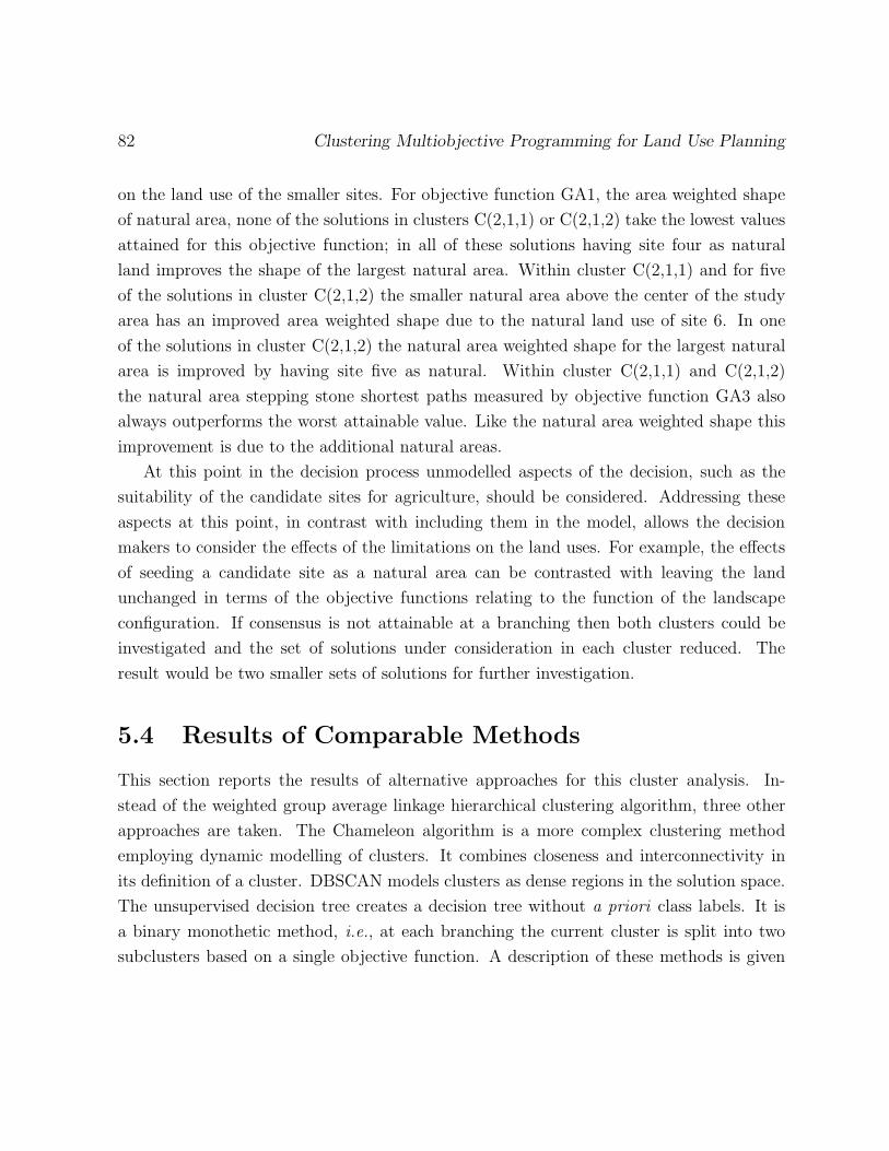
82 Clustering Multiobjective Programming for Land Use Planning
on the land use of the smaller sites. For objective function GA1, the area weighted shape
of natural area, none of the solutions in clusters C(2,1,1) or C(2,1,2) take the lowest values
attained for this objective function; in all of these solutions having site four as natural
land improves the shape of the largest natural area. Within cluster C(2,1,1) and for five
of the solutions in cluster C(2,1,2) the smaller natural area above the center of the study
area has an improved area weighted shape due to the natural land use of site 6. In one
of the solutions in cluster C(2,1,2) the natural area weighted shape for the largest natural
area is improved by having site five as natural. Within cluster C(2,1,1) and C(2,1,2)
the natural area stepping stone shortest paths measured by objective function GA3 also
always outperforms the worst attainable value. Like the natural area weighted shape this
improvement is due to the additional natural areas.
At this point in the decision process unmodelled aspects of the decision, such as the
suitability of the candidate sites for agriculture, should be considered. Addressing these
aspects at this point, in contrast with including them in the model, allows the decision
makers to consider the effects of the limitations on the land uses. For example, the effects
of seeding a candidate site as a natural area can be contrasted with leaving the land
unchanged in terms of the objective functions relating to the function of the landscape
configuration. If consensus is not attainable at a branching then both clusters could be
investigated and the set of solutions under consideration in each cluster reduced. The
result would be two smaller sets of solutions for further investigation.
5.4 Results of Comparable Methods
This section reports the results of alternative approaches for this cluster analysis. In-
stead of the weighted group average linkage hierarchical clustering algorithm, three other
approaches are taken. The Chameleon algorithm is a more complex clustering method
employing dynamic modelling of clusters. It combines closeness and interconnectivity in
its definition of a cluster. DBSCAN models clusters as dense regions in the solution space.
The unsupervised decision tree creates a decision tree without a priori class labels. It is
a binary monothetic method, i.e., at each branching the current cluster is split into two
subclusters based on a single objective function. A description of these methods is given
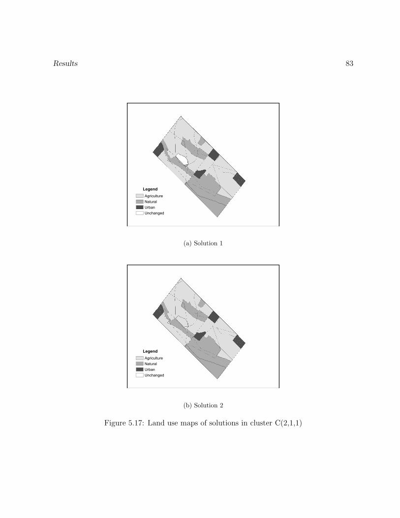
Results 83
Legend
Agriculture
Natural
Urban
Unchanged
(a) Solution 1
Legend
Agriculture
Natural
Urban
Unchanged
(b) Solution 2
Figure 5.17: Land use maps of solutions in cluster C(2,1,1)
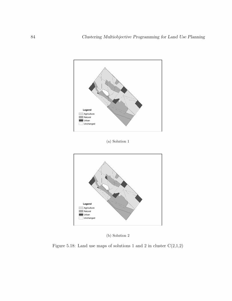
84 Clustering Multiobjective Programming for Land Use Planning
Legend
Agriculture
Natural
Urban
Unchanged
(a) Solution 1
Legend
Agriculture
Natural
Urban
Unchanged
(b) Solution 2
Figure 5.18: Land use maps of solutions 1 and 2 in cluster C(2,1,2)
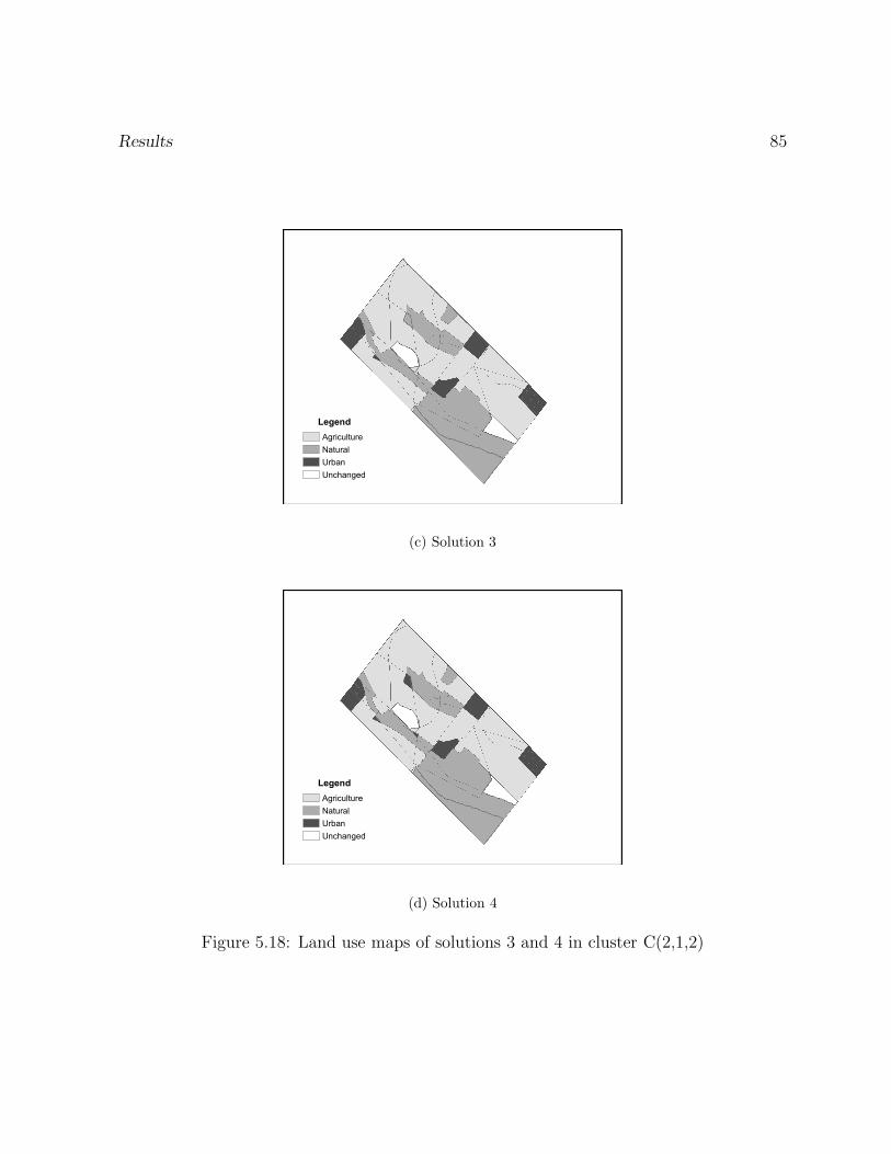
Results 85
Legend
Agriculture
Natural
Urban
Unchanged
(c) Solution 3
Legend
Agriculture
Natural
Urban
Unchanged
(d) Solution 4
Figure 5.18: Land use maps of solutions 3 and 4 in cluster C(2,1,2)
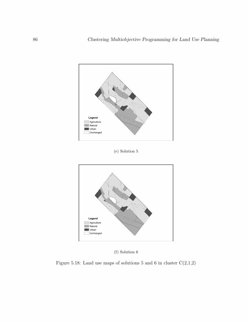
86 Clustering Multiobjective Programming for Land Use Planning
Legend
Agriculture
Natural
Urban
Unchanged
(e) Solution 5
Legend
Agriculture
Natural
Urban
Unchanged
(f) Solution 6
Figure 5.18: Land use maps of solutions 5 and 6 in cluster C(2,1,2)
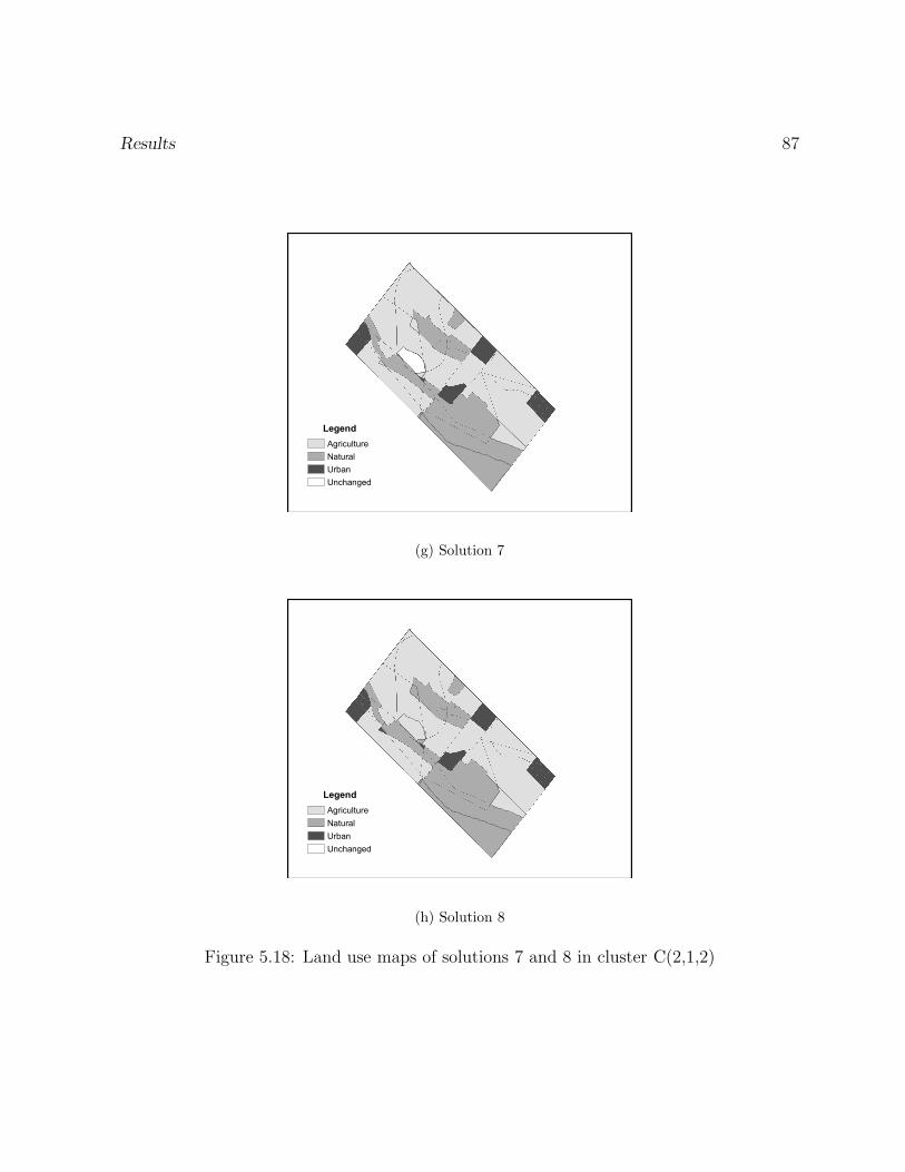
Results 87
Legend
Agriculture
Natural
Urban
Unchanged
(g) Solution 7
Legend
Agriculture
Natural
Urban
Unchanged
(h) Solution 8
Figure 5.18: Land use maps of solutions 7 and 8 in cluster C(2,1,2)
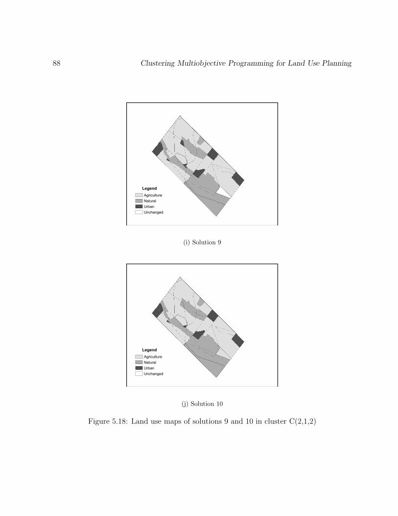
88 Clustering Multiobjective Programming for Land Use Planning
Legend
Agriculture
Natural
Urban
Unchanged
(i) Solution 9
Legend
Agriculture
Natural
Urban
Unchanged
(j) Solution 10
Figure 5.18: Land use maps of solutions 9 and 10 in cluster C(2,1,2)
Results 89
in section 2.4.3.
5.4.1 Chameleon
Chameleon merges the 16 partitions of the k-nearest neighbour graph into the tree shown
in figure 5.19. The results of Chameleon are shown as plotmatrices in appendix C. These
partitions are numbered P1 through P16. This tree differs from the results of the hierar-
chical clustering algorithms and the other comparable methods in that the leaves are not
individual solutions; the solutions cannot be partitioned more finely than the partitioning
of the k-nearest neighbour graph. For example cluster C(1,1) is partition P1. There are 13
solutions in this cluster which cannot be further divided in these results. Five of the leaves
occur after only three or fewer branchings; these are clusters C(1,1), C(1,2,1), C(1,2,2),
C(2,1,1), and C(2,1,2).
Chameleon does not detect the three major clusters even after three branchings. Cluster
C(2,2,2), shown in figure 5.20, contains solutions from each of the three major clusters.
The trade-off for area between the three land uses is not detected by Chameleon even
though it is a significant part of the landscape design problem.
One strength of the hierarchical linkage method is that it provides clearly differentiated
clusterings even where there is no discernible cluster structure. In the lower parts of the
dendrograms the solutions are highly similar but the algorithm is always able to provide
a clearly interpretable branching. Chameleon has two weaknesses in this regard. First, it
cannot branch the solutions any more finely than the k-nearest neighbour graph partition-
ing. Second, some of the branchings lack interpretability in the plotmatrix and value path
plots. For example, clusters C(2,2,1) and C(2,2,2) appear to overlap in all of the objective
function plots in figure 5.20.
Even if the results of Chameleon were as good as the weighted group average hierarchical
linkage results, the complexity of Chameleon makes it undesirable for this application for
two reasons. First, the many interacting parameters require fine-tuning in order to obtain
good results. It is unlikely that Chameleon could be automated and included in a decision
support system without requiring in depth knowledge of the algorithm by an analyst using
the system. Second, decision makers in land use planning require an understanding of the
analysis in order to be accountable and responsible. Increased complexity makes it the
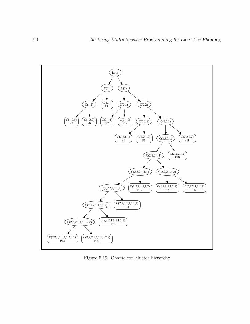
90 Clustering Multiobjective Programming for Land Use Planning
Root
C(1) C(2)
C(1,2)C(1,1)
P1C(2,1) C(2,2)
C(1,2,1)P3
C(1,2,2)P6
C(2,1,1)P2
C(2,1,2)P12
C(2,2,1) C(2,2,2)
C(2,2,1,1)P5
C(2,2,1,2)P9
C(2,2,2,1)C(2,2,2,2)
P11
C(2,2,2,1,1)C(2,2,2,1,2)
P10
C(2,2,2,1,1,1) C(2,2,2,1,1,2)
C(2,2,2,1,1,1,1)C(2,2,2,1,1,1,2)
P15C(2,2,2,1,1,2,1)
P7C(2,2,2,1,1,2,2)
P13
C(2,2,2,1,1,1,1,2)C(2,2,2,1,1,1,1,1)
P4
C(2,2,2,1,1,1,1,2,2)C(2,2,2,1,1,1,1,2,1)
P8
C(2,2,2,1,1,1,1,2,2,1)P14
C(2,2,2,1,1,1,1,2,2,2)P16
Figure 5.19: Chameleon cluster hierarchy
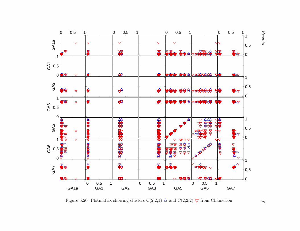
Resu
lts91
0
0.5
1
GA70 0.5 1
GA6
GA50 0.5 1
GA3
GA20 0.5 1
GA1
GA1a
GA
7
0
0.5
1
GA
6
0
0.5
1
GA
5
0
0.5
1
GA
3
0
0.5
1
GA
2
0
0.5
1
GA
1
0 0.5 1
0
0.5
10 0.5 10 0.5 10 0.5 1
GA
1a
Figure 5.20: Plotmatrix showing clusters C(2,2,1) 4 and C(2,2,2) 5 from Chameleon
92 Clustering Multiobjective Programming for Land Use Planning
system more likely to be a ‘black box’ to the end users.
5.4.2 DBSCAN
Figure 5.21 is a tree showing the clustering hierarchy resulting from using DBSCAN. If
at a branching it was necessary to adjust the value of Eps, the distance defining the
neighbourhood around a point, from the automated calculation the final value is shown
within the node being branched. It is also necessary to specify k, the number of points
required to define a dense region. The appropriate value of k depends on the data set
characteristics such as the dimensionality and densities. The manual adjustment of Eps
is an additional complication necessary in DBSCAN compared to the hierarchical linkage
clustering methods and is required in five of the ten branchings performed. At the root the
automated value of Eps resulted in three nodes, C(1), C(2), and C(3); with the default
setting DBSCAN detected the three major clusters as seen in figure 5.22. Unlike the
hierarchical linkage clustering methods no indication of the relative importance of the
branchings, e.g., the dendrogram heights, is available but three-way branchings can occur
where two consecutive branchings are of nearly the same importance. At node C(1,1),
where Eps = 0.02, three clusters resulted after adjusting Eps to obtain more than a
single cluster. Cluster C(3,1) contains only two solutions and cannot be branched using
DBSCAN since there must be more than one solution in each dense region defining a
subcluster. Appendix D contains plotmatrices of each branching shown in figure 5.21.
In some cases it is difficult to find a value of Eps that results in more than a single
cluster. Unlike the hierarchical linkage clustering methods DBSCAN did not easily adapt
to the smaller and more compact clusters resulting after several branchings; the three
major clusters are easily detected but it is necessary to manually adjust the value of Eps
in some cases where no obvious subcluster structure exists.
The clustering structure resulting from DBSCAN can be assessed based on the decision
example scenario in section 5.3. At the first branching the three major clusters are obvious.
Cluster C(1) is the most desirable since it contains the solutions with high values of the
natural land use area objective function, GA1a. This selection eliminates all solutions with
high values of urban area, GA7, from consideration.
Within cluster C(3), shown in figure 5.23, there are two subclusters. These subclusters
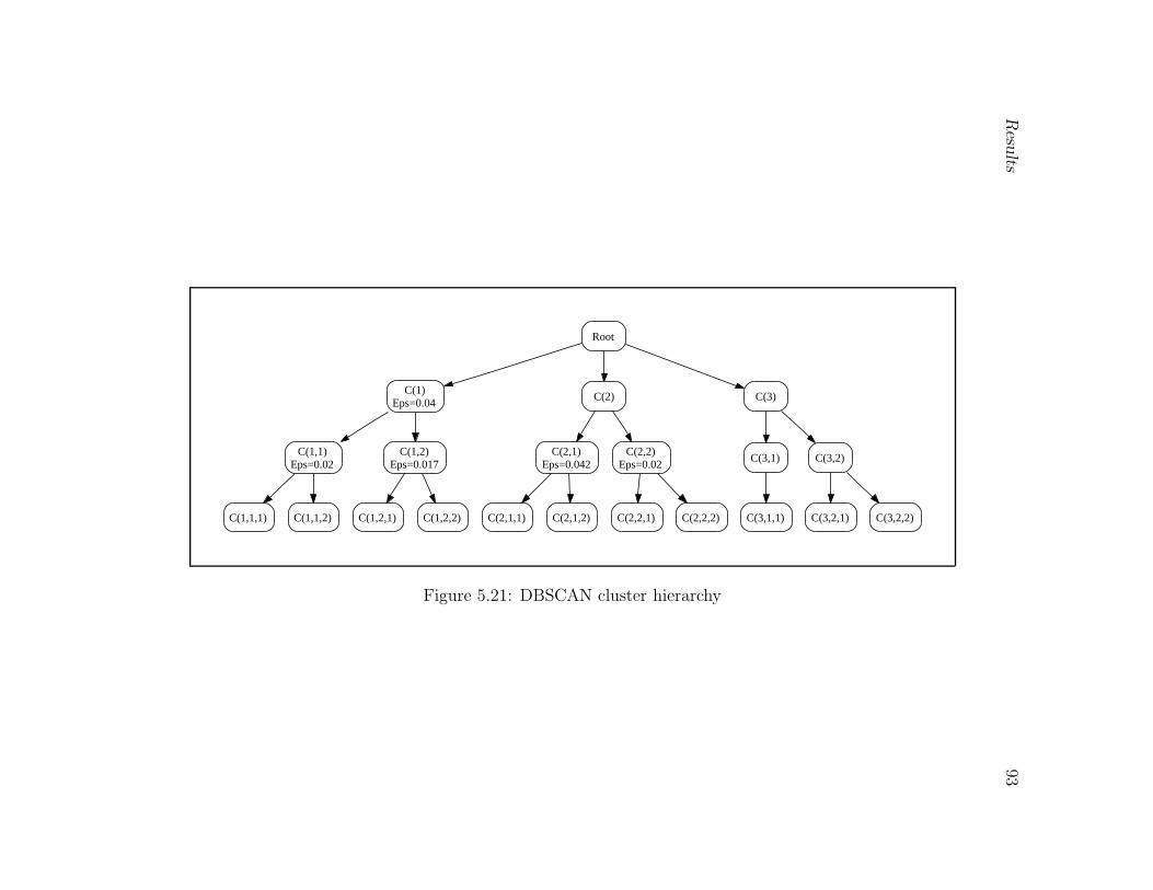
Resu
lts93
Root
C(1)Eps=0.04
C(2) C(3)
C(1,1)Eps=0.02
C(1,2)Eps=0.017
C(2,1)Eps=0.042
C(2,2)Eps=0.02
C(3,1) C(3,2)
C(1,1,1) C(1,1,2) C(1,2,1) C(1,2,2) C(2,1,1) C(2,1,2) C(2,2,1) C(2,2,2) C(3,1,1) C(3,2,1) C(3,2,2)
Figure 5.21: DBSCAN cluster hierarchy
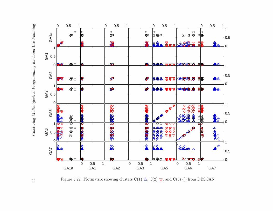
94C
lust
erin
gM
ult
iobje
ctiv
eP
rogra
mm
ing
for
Land
Use
Pla
nnin
g
0
0.5
1
GA70 0.5 1
GA6
GA50 0.5 1
GA3
GA20 0.5 1
GA1
GA1a
GA
7
0
0.5
1
GA
6
0
0.5
1
GA
5
0
0.5
1
GA
3
0
0.5
1
GA
2
0
0.5
1G
A1
0 0.5 1
0
0.5
10 0.5 10 0.5 10 0.5 1
GA
1a
Figure 5.22: Plotmatrix showing clusters C(1) 4, C(2) 5, and C(3) © from DBSCAN
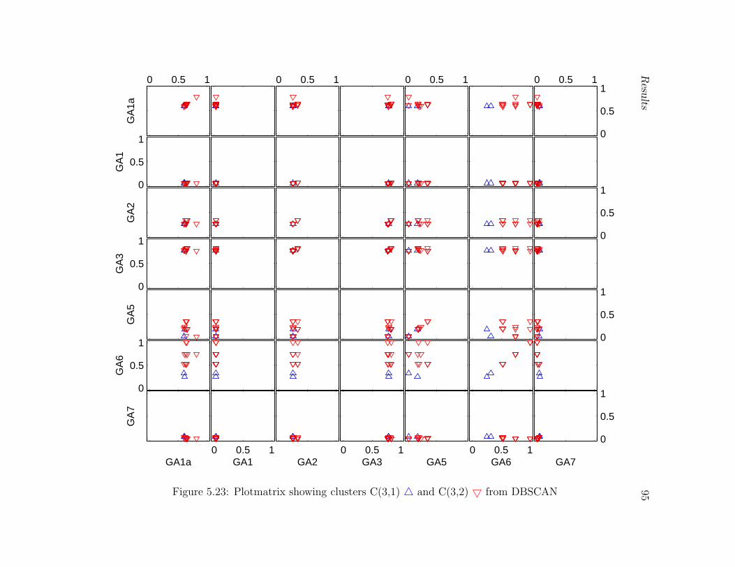
Resu
lts95
0
0.5
1
GA70 0.5 1
GA6
GA50 0.5 1
GA3
GA20 0.5 1
GA1
GA1a
GA
7
0
0.5
1
GA
6
0
0.5
1
GA
5
0
0.5
1
GA
3
0
0.5
1
GA
2
0
0.5
1
GA
1
0 0.5 1
0
0.5
10 0.5 10 0.5 10 0.5 1
GA
1a
Figure 5.23: Plotmatrix showing clusters C(3,1) 4 and C(3,2) 5 from DBSCAN
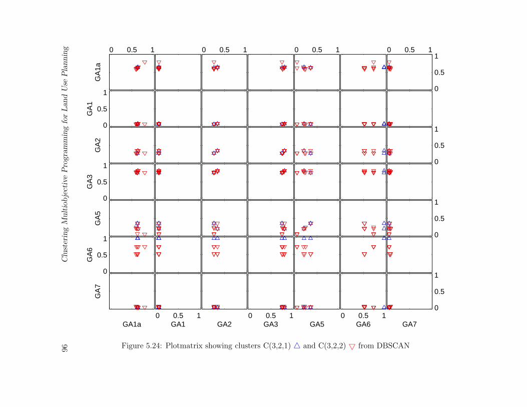
96C
lust
erin
gM
ult
iobje
ctiv
eP
rogra
mm
ing
for
Land
Use
Pla
nnin
g
0
0.5
1
GA70 0.5 1
GA6
GA50 0.5 1
GA3
GA20 0.5 1
GA1
GA1a
GA
7
0
0.5
1
GA
6
0
0.5
1
GA
5
0
0.5
1
GA
3
0
0.5
1
GA
2
0
0.5
1G
A1
0 0.5 1
0
0.5
10 0.5 10 0.5 10 0.5 1
GA
1a
Figure 5.24: Plotmatrix showing clusters C(3,2,1) 4 and C(3,2,2) 5 from DBSCAN
Results 97
are differentiated on objective function GA6, clustered development. Cluster C(3,1) takes
the lower values of clustered development and cluster C(3,2) takes the higher values. The
maximal values of GA1a, natural land area, and GA2, natural connectivity, occur only in
cluster C(3,2). Cluster C(3,2) is preferable according to the decision scenario.
As in cluster C(3), the subclusters of cluster C(3,2), shown in figure 5.24, differ primarily
in objective function GA6, clustered development. The highest value for objective function
GA1a, natural land area, trades off with the highest value for objective function GA6,
clustered development. Clusters C(3,2,1) and C(3,2,2) are the same as cluster C(2,1,1)
and C(2,1,2) from the weighted group average linkage method as shown in figure 5.5.
DBSCAN allows branchings resulting in more than two clusters which may more ac-
curately depict certain cluster structures, for example, the three major clusters in the
landscape configuration problem. Like Chameleon, DBSCAN is more complicated than
the hierarchical linkage clustering algorithms. DBSCAN requires the specification of a
parameter, Eps. While there is a formula available to calculate a default value of Eps for
each branching at some branchings it is necessary to manually adjust Eps to obtain more
than one subcluster. Although it is a more complicated method for the example decision
DBSCAN selects the same solutions for further consider as the proposed methodology.
5.4.3 Unsupervised Decision Tree
Figure 5.25 shows the unsupervised decision tree for the NSGA-II results. Each branching
is labeled with the test based on a single objective function to define that branching. The
existence of three major clusters is unclear from this tree. At the first branching two of the
major clusters are contained in cluster C(1) and the other major cluster is cluster C(2).
Even though the two major clusters in cluster C(1) can be differentiated based on a single
objective function, GA1a, the unsupervised decision tree algorithm does not split them at
the next branching. Clusters C(1,1) and C(1,2), as well as C(1,1,1), C(1,1,2), C(1,2,1), and
C(1,2,2), contain elements from two of the major clusters. These two of the three major
clusters are not uncovered even after three branchings.
The objective function used at the first branching is GA5, agricultural land area. From
figure 5.26 it can be seen that cluster C(2) contains only sites with low values for the
natural land use objective functions. Thus, based on the scenario in the example decision
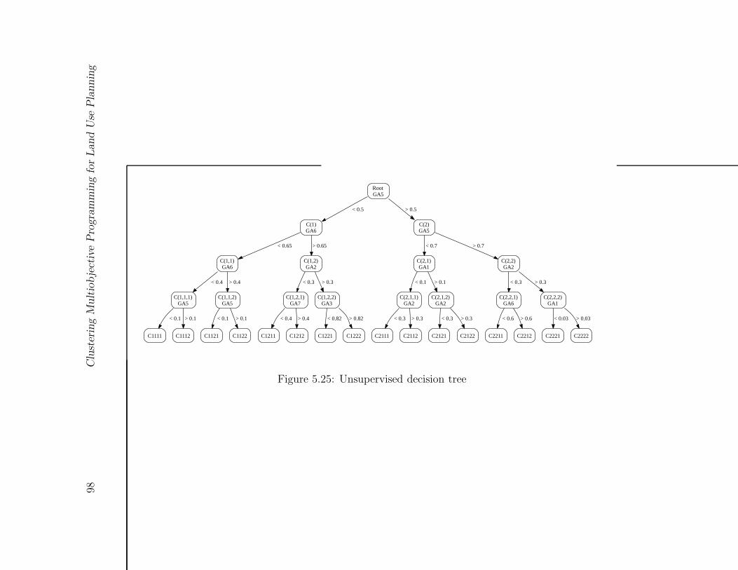
98C
lust
erin
gM
ult
iobje
ctiv
eP
rogra
mm
ing
for
Land
Use
Pla
nnin
g
RootGA5
C(1)GA6
< 0.5
C(2)GA5
> 0.5
C(1,1)GA6
< 0.65
C(1,2)GA2
> 0.65
C(2,1)GA1
< 0.7
C(2,2)GA2
> 0.7
C(1,1,1)GA5
< 0.4
C(1,1,2)GA5
> 0.4
C(1,2,1)GA7
< 0.3
C(1,2,2)GA3
> 0.3
C(2,1,1)GA2
< 0.1
C(2,1,2)GA2
> 0.1
C(2,2,1)GA6
< 0.3
C(2,2,2)GA1
> 0.3
C1111
< 0.1
C1112
> 0.1
C1121
< 0.1
C1122
> 0.1
C1211
< 0.4
C1212
> 0.4
C1221
< 0.82
C1222
> 0.82
C2111
< 0.3
C2112
> 0.3
C2121
< 0.3
C2122
> 0.3
C2211
< 0.6
C2212
> 0.6
C2221
< 0.03
C2222
> 0.03
Figure 5.25: Unsupervised decision tree
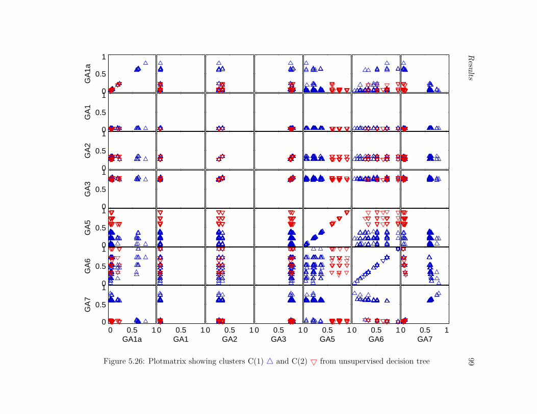
Resu
lts99
0 0.5 1GA7
0 0.5 1GA6
0 0.5 1GA5
0 0.5 1GA3
0 0.5 1GA2
0 0.5 1GA1
0 0.5 10
0.5
1
GA1a
GA
7
0
0.5
1
GA
6
0
0.5
1
GA
5
0
0.5
1
GA
3
0
0.5
1
GA
2
0
0.5
1G
A1
0
0.5
1
GA
1a
Figure 5.26: Plotmatrix showing clusters C(1) 4 and C(2) 5 from unsupervised decision tree
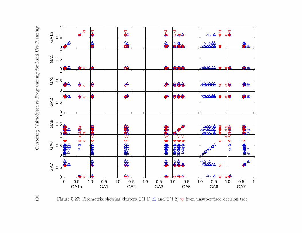
100
Clu
ster
ing
Mult
iobje
ctiv
eP
rogra
mm
ing
for
Land
Use
Pla
nnin
g
0 0.5 1GA7
0 0.5 1GA6
0 0.5 1GA5
0 0.5 1GA3
0 0.5 1GA2
0 0.5 1GA1
0 0.5 10
0.5
1
GA1a
GA
7
0
0.5
1
GA
6
0
0.5
1
GA
5
0
0.5
1
GA
3
0
0.5
1
GA
2
0
0.5
1G
A1
0
0.5
1
GA
1a
Figure 5.27: Plotmatrix showing clusters C(1,1) 4 and C(1,2) 5 from unsupervised decision tree
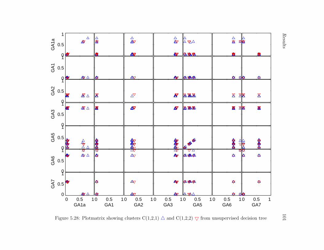
Resu
lts101
0 0.5 1GA7
0 0.5 1GA6
0 0.5 1GA5
0 0.5 1GA3
0 0.5 1GA2
0 0.5 1GA1
0 0.5 10
0.5
1
GA1a
GA
7
0
0.5
1
GA
6
0
0.5
1
GA
5
0
0.5
1
GA
3
0
0.5
1
GA
2
0
0.5
1G
A1
0
0.5
1
GA
1a
Figure 5.28: Plotmatrix showing clusters C(1,2,1) 4 and C(1,2,2) 5 from unsupervised decision tree

102 Clustering Multiobjective Programming for Land Use Planning
in section 5.3, none of the solutions in cluster C(2) are desirable. While these solutions
contains significant new natural area, the new agricultural area is less than 50% of the
total area of the candidate sites.
The decision at the second branching as shown in figure 5.27 is whether GA6, clustered
development, should be greater than 0.65. Since, based on the decision scenario described,
it is desirable to increase this objective function and neither of the subclusters limit the
attainable values of the other objective functions,, the higher value of GA6 would be chosen.
That choice leads to cluster C(1,2) and the third branching decision: whether GA2,
natural connectivity, should be greater than 0.3. The values of GA2 differ little within
cluster C(1,2) but it is selected for branching even though much more significant variability
exists within GA1a, natural area. Again there is no obvious relationships between the
branching objective function and the other objective functions within the cluster, as seen
in figure 5.28. The higher values of GA2 are more desirable so cluster C(1,2,2) should be
selected.
After three branchings the landscape designs under consideration contained wide ranges
of values for the land use area objective functions, GA1a, GA5, and GA7, as well as for
clustered development, GA6. Some of the solutions selected for further consideration using
the unsupervised decision tree are in cluster C(2,1,1) selected for further consideration in
the proposed methodology shown in figure 5.5. The set of solutions selected for further
consideration also contains some solutions that different significantly from those in the
weighted group average cluster C(2,1,1) in terms of objective functions GA1a, GA6, and
GA7, the natural land area, the clustered development, and urban land area.
The structure resulting from the unsupervised decision tree approach did not address
the aim of identifying the three major clusters; after three branchings the solutions chosen
for further consideration still contained solutions in two of the major clusters. These
solutions vary significantly in two objective functions known to conflict, GA1a and GA7,
the natural and urban land areas, respectively.
This chapter presented the results of the proposed cluster analysis methodology as well
as tests of internal, external, and relative validity. The results of the proposed methodology
are sufficiently valid. It also detailed an example decision using the results of the proposed

Results 103
methodology leading to the selection of a small set of solutions for further consideration.
The results of three comparable methods were also presented. Two of the comparable
methods, Chameleon and the unsupervised decision tree method, do not yield a suitable
representation of the NSGA-II results. The remaining comparable method, DBSCAN,
gives similar results to the proposed methodology although it allows three-way branchings.
DBSCAN is more complex and requires the manual adjustment of a parameter to ensure
good performance; thus it is less suitable than the proposed methodology. Chapter 6 dis-
cusses the results presented in this chapter including potential reuse for other applications
and inclusion in a decision support system. The last chapter presents conclusions and
recommendations for future work.

Chapter 6
Discussion
This chapter begins with a discussion of the proposed cluster analysis methodology in
terms of the quality and usefulness of the resulting structure for the landscape configu-
ration problem. It then addresses the suitability of the proposed methodology for other
applications, both for reusing the methodology with other data sets or applications and
employing the methodology as part of a decision support system (DSS) for multiobjective
optimization problems.
The weighted group average linkage hierarchical clustering method was largely success-
ful for this application. There are three primary aims for the proposed methodology. First,
it should create a tractable presentation of the NSGA-II results for the landscape configu-
ration problem. As noted in section 5.1.3, visually obvious clusters should be detected and
a useful structure should be provided even where no obvious structure exists. The validity
of the resulting structure is also important. This aim is discussed in section 6.1. Second,
it should be adaptable to other problems suited to a multiobjective optimization frame-
work using Pareto front enumeration or approximation methods. This second requirement
includes being extendable to include other model aspects such as constraints, preferences,
and weights. This aim is discussed in section 6.2.1. Third, it should be amenable to future
inclusion in a decision support system (DSS). This aim is discussed in section 6.2.2.
105
106 Clustering Multiobjective Programming for Land Use Planning
6.1 Discussion of Results and Validity
The proposed methodology successfully detects the three major clusters as clusters C(1),
C(2,1), and C(2,2). Two branchings are required to detect the three major clusters since
the weighted group average hierarchical linkage method allows only two subclusters to exist
at a branching. As per section 5.2, the results are a reasonable representation of the input
data with respect to internal, external, and relative validity.
Some sets of consecutive branchings in the dendrogram occur at similar heights. In such
cases the branchings could be merged without significantly changing the interpretation
and potentially increasing the clarity of the presentation of the cluster structure. In the
landscape configuration problem merging the first two branchings would give one three-
way branching at the top of the dendrogram; at the root three clusters would be presented
instead of two, i.e., clusters C(1), C(2), and C(3) would be the three major clusters instead
of clusters C(1), C(2,1), and C(2,2). This structure would more accurately reflect the
trade-off between the land use objective functions. As well, allowing three-way or n-way
branchings in the tree could result in a more compact tree, since the number of branchings
would be reduced, but doing so would force the decision makers to consider more than
two alternatives at once. Further investigation is needed to assess whether this type of
structure would be desirable for some applications or whether the dendrogram should be
accompanied by a note emphasizing the meaning of the heights more clearly.
In the first few branchings of the dendrogram the clusters correspond to those noted in
the visual inspection for clustering tendency. The branchings lower in the dendrogram do
not correspond to visually obvious clusters since no obvious clusters exist. These branchings
segment the obvious clusters into sub-clusters that are differentiated but not significantly
separated. The use of a hierarchical linkage clustering algorithm allows the method to deal
with these branchings where there may be no cluster structure and return usable results.
As discussed in section 5.4, Chameleon is unable to adapt to these regions and DBSCAN
requires fine-tuning to return the desired results.
In the first three branchings the resulting clusters are not differentiated on objective
functions GA1, the area weighted mean shape of the core natural areas, GA2, the natural
features connectivity, and GA3, the stepping stones of natural features on shortest paths.
This behaviour occurs due to the small range of values taken by each of these objective
Discussion 107
functions. The Euclidean distance measure embedded in the average linkage hierarchical
clustering method emphasizes larger distances. If these objective functions are key com-
ponents of the decision then this behaviour is undesirable and the structure returned by
the unsupervised decision tree is preferable. This behaviour could be changed by rescaling
these objective functions to reflect their importance. This rescaling was not done as the
objective functions could potentially have values ranging from 0 to 1. The limitations of
the existing landscape prevent most of that range from being attainable. This rescaling
would add an additional step to the proposed methodology where the relative ranges of the
objective functions must be considered and linearly rescaled in order to reflect their rela-
tive importance. Since it is undesirable to make such value judgments before exploring the
possibilities existing on the Pareto front, this step should be used after the methodology
has been applied and the cluster analysis should be repeated. A difficulty that may result
is achieving consensus from the decision makers regarding the appropriate selection and
scaling of the objective functions but this methodology is proposed as a tool to tractably
consider the efficient solutions; it does not determine whether one objective function is
more important than any other objective function but uses them in a simple manner in or-
der to organize the results. If an objective function is clearly very important than it should
be employed by the cluster analysis. Alternatively, this behaviour could be changed by
using a different distance measure but this approach may complicate the method and in-
volves more explicitly considering the relationships between the objective functions. The
initial results of the cluster analysis will inform later formulations of the problem making
this approach more desirable than a priori value judgments such as specifying weights or
goals for objective functions.
The binary branching structure in the dendrogram allows the set of solutions to be
considered based on their objective function values. Potentially interesting subsets of
solutions for further consideration can be found by reducing the set under consideration
by descending in the tree from the root until a sufficiently small set of solutions with
sufficiently similar objective function values remains. Using the dendrogram resulting
from the weighted group average linkage method the set under consideration can be made
arbitrarily small. Since the tree is not balanced the decrease in the number of solutions
under consideration resulting from each branching is not predictable and many branchings
108 Clustering Multiobjective Programming for Land Use Planning
may need to be taken in order to obtain a sufficiently small set. If that were the case
then another hierarchical linkage method, such as the complete linkage method, could be
employed to return a dendrogram that is more balanced but less indicative of the trade-off
surface structure.
The proposed methodology provides a tractable representation of the multiobjective
optimization results. While the effects of the relative ranges of the objective functions
may complicate the use of this methodology or implicitly convey additional importance
to a particular objective function, currently available methods do not consider multiple
objective functions simultaneously without some consideration of the relative importance
of the objective functions or other a priori value judgments. NSGA, NSGA-II, and other
multiobjective optimization algorithms may give good results for problems with objective
functions of different scales but they often include an implicit rescaling or assumption
that the objective functions are similarly scaled. For example, within NSGA the sharing
parameter defines a hypersphere in the objective function space within which solutions
are deemed ‘close’ and thus have their fitness values degraded. This hypersphere has
the same radius along each objective function. In NSGA-II the sharing parameter is
replaced by the crowding distance calculation. In the crowding distance each objective
function is linearly rescaled by mapping the current sample range to [0, 1]. The rescaled
objective function values are used to calculate the largest cuboid containing each solution
that contains no other solutions. The solutions are then ranked according to the dimensions
of their cuboids. In addition to this implicit assumption regarding the scales of the objective
functions, in this thesis the cluster structure emphasizes those objective functions that
clearly differentiate the clusters occurring higher in the dendrogram.
6.2 Suitability for Reuse and Extension
There are two aspects to the generalizability of the proposed methodology. First, whether
this cluster analysis methodology could be adapted for other multiobjective problems.
This aspect includes applying it to other datasets resulting from Pareto front enumeration
or approximation methods as well as extending it to include other modelling tools such
as constraints, preferences, or weights. Second, the suitability of this methodology for
Discussion 109
inclusion in decision support systems (DSS), particularly spatial DSS (SDSS) and planning
support systems (PSS).
6.2.1 Suitability for Reuse
The steps involved in the cluster analysis methodology are acquiring the input data, es-
tablishing a clustering tendency, data preparation and scaling, selection of a proximity
measure, choice of a clustering algorithm, application of the clustering algorithm, and val-
idation. This section discusses the requirements for each of these steps in order to apply
this methodology to a different data set or application. It also notes the limitations of the
methodology imposed by each step.
The characteristics of the input data are important to the use and success of this
methodology. The proposed methodology is most easily applied where the input data
is the result of a Pareto front enumeration or approximation algorithm and a clustering
tendency can clearly be seen in two-dimensional visualizations. If the decision variables in
the multiobjective optimization problem are continuous, as opposed to discrete as in the
landscape configuration problem, the input to the clustering algorithm must be a discrete
approximation of the Pareto front. A multiobjective programming solution algorithm that
returns functions approximating the Pareto front could be used only if the functions were
sampled to generate a discrete approximation.
If the problem has only two or three objective functions, and in particular if those
functions are well-behaved, there is little benefit to using the proposed methodology. If a
simple two or three dimensional visualization of the Pareto front or a good approximation
thereof is available the proposed methodology cannot lead to additional insight. The
proposed methodology is particularly useful where there are more than three objective
functions but not so many objective functions that it becomes difficult to select one of the
clusters at a branching.
One potential application is engineering design. In these problems there are often
many parameters to be specified. These parameters can be specified a priori or modelled
with objective functions, e.g., minimizing the weight of an airplane wing and the cost of
material while maximizing the lift and the rigidity. In a single objective framework, one
or more of these parameters would be combined to form the objective function. Goal
110 Clustering Multiobjective Programming for Land Use Planning
values or ranges would be specified for the other parameters to model them as constraints.
Using multiobjective optimization and the methodology developed in this thesis, the range
of different Pareto optimal designs and the interaction between the parameters can be
considered before formulating the specifications for the wing.
A second potential application is portfolio selection in financial optimization. Portfolio
selection problems consider a set of criteria in order to select a good portfolio, where the
meaning of good depends on the criteria chosen. For example, the variance, as a measure of
risk, and the expected return are commonly used. Considering additional criteria, such as
Value-at-Risk (VaR) and expected shortfall, would provide additional information about
the quality of the portfolios. These criteria can be modelled as multiple objective and the
methodology presented in this thesis used to consider the possible values and interactions.
The proposed methodology is best applied where there is a clustering tendency in
the input data. If the decision variables of the multiobjective optimization problem are
continuous then the concept of density across the Pareto front has no meaning. If the
decision variables are continuous then the input data to the proposed methodology should
sample the Pareto front uniformly. A non-uniform sample could be used but the resulting
cluster structure would reflect the varying sample density across the trade-off surface. If
the decision variables are discrete the Pareto front, which will then be discrete as well, may
have a constant density. Again, care should be taken to ensure that this constant density
is reflected in the input data to the clustering algorithm. In this case, as with continuous
decision variables, unless there are several components to the Pareto front in different
regions of the objective function space there will be no cluster structure. In either case, even
if there are segments of the Pareto front in different regions of the objective function space
resulting in a set of clusters it is unlikely that there will be sets of segments within each of
those regions and subsets of segments within those sets leading to a hierarchical clustering
structure. Again it is important to consider a two- or three-dimensional projection of the
input data to consider its structure. If the decision variables are continuous or discrete with
a constant density and a good approximation of the Pareto front is easily obtained then
the approach taken by Mattson et al. (2004) described in section 2.2 to find ‘interesting’
regions of the Pareto front may be more suitable. Applying the methodology proposed in
this thesis may still yield insight for these problems, particularly if it is difficult to obtain
Discussion 111
a good approximation of the Pareto front. If no clustering tendency exists it should be
acknowledged that any structure resulting from the application of a clustering algorithm
will be an artifact of that clustering algorithm. Nonetheless, a clustering algorithm could
be used to objectively construct a tractable representation using a dendrogram.
Data preparation, in particularly scaling of the objective functions to remove implicit
bias toward the objective functions with larger ranges, must be repeated for any new data
set or any other application. The linear range scaling used in this thesis performs well
for recovering clustering structure without imposing additional assumptions regarding the
processes generating the data, as noted in section 4.1.2. If the data is known to have been
generated from a statistical process, such as a mixture of Gaussian processes, and good esti-
mates of the shapes of the clusters are available then scaling using the variance or standard
deviation may be suitable. If the data is known to follow a statistical distribution then an
alternate clustering method should be used that takes advantage of that knowledge. The
methodology described in the thesis may yield useful results in those cases but additional
insight may be available by taking all the known information, including the distributions or
generation processes, into account. The methodology developed in this thesis is primarily
concerned with discrete data points resulting from multiobjective optimization without an
obvious generating process.
The selection of a suitable proximity measure may change with the input data. As
discussed in section 4.1.3, the Euclidean distance is a robust measure that is easily inter-
preted. It is commonly used and suitable for many data sets. A major shortcoming of the
Euclidean distance is a sensitivity to the relative scales of the objective functions which
must be address as described in the previous paragraph.
Section 4.1.4 begins by considering the centroid method, Ward’s method, the complete
linkage method, and the weighted group average method as candidate hierarchical cluster-
ing methods for use in this methodology. Each of these methods were found to work well in
similar studies. The centroid method is found to give reversals, reducing the interpretabil-
ity of the results. It should not be used due to this possibility. Ward’s method assumes
spherical balanced clusters and the complete linkage method assumes balanced clusters.
The weighted group average linkage method selected makes the fewest assumptions about
the characteristics of the clusters. If when considering the clustering tendency the clusters

112 Clustering Multiobjective Programming for Land Use Planning
are seen to be spherical or balanced then Ward’s method or the complete linkage method
may be considered although the weighted average linkage method may perform as well. The
weighted average linkage method should be used if there is no obvious reason to employ
another hierarchical linkage method.
The application of the selected clustering algorithm, likely the weighted average hi-
erarchical linkage method, can be performed by a number of software packages or can
be coded based on the material in section 2.4.2. Some software packages implementing
clustering algorithms include SPSS, Matlab (with the Statistical Toolbox), and the open
source packages Cluster and R (with the Stats Package). Seo and Shneiderman (2002) dis-
cusses several hierarchical clustering software packages used in genomics with an emphasis
on visualization. Hierarchical linkage-based cluster algorithms do not require any input
parameters. A dendrogram is the typical output visualizations and individual branchings
can be considered using other visualization such as value path plots or plotmatrices. The
suitability of the proposed methodology within a decision support system is described in
the next section.
6.2.2 Suitability for Decision Support Systems
The proposed method aims to inform decision making in discrete multiobjective optimiza-
tion.
The dendrogram representing the cluster structure can be used as in the example de-
cision in section 5.3. An alternative approach is to consider the dendrogram as a binary
tree and at each branching to consider whether either of the two branches can be pruned.
Pruning a branch removes the solutions in that cluster from consideration. Once a branch
has been pruned the branchings deeper in that cluster need not be considered. The result
of this process may be a single cluster of interest that remains after pruning is complete
or a reduced binary tree where fewer of the branchings remain than were initially under
consideration. If a reduced tree is obtained then there are several clusters of solutions that
merit further consideration and the tree shows how these clusters are related.
Once a hierarchical clustering structure is obtained, the dendrogram can be used in de-
cision support systems. The dendrogram may be enhanced by simultaneous display with
other visualizations. Seo and Shneiderman (2002) present uses for dendrograms in explor-
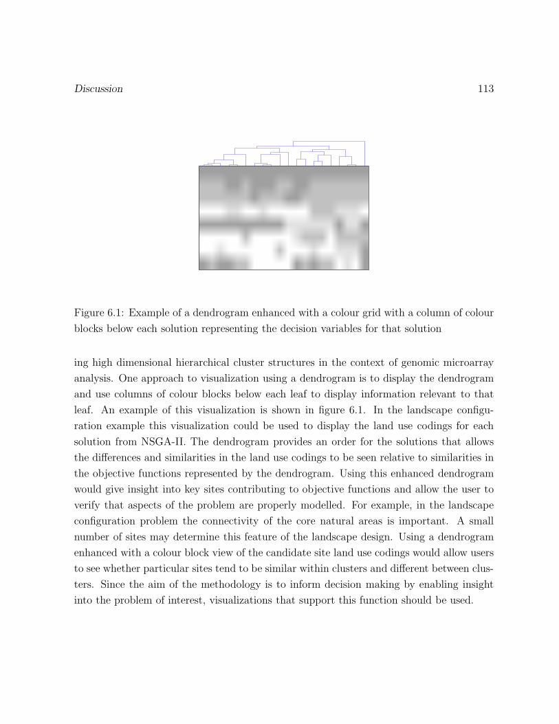
Discussion 113
Figure 6.1: Example of a dendrogram enhanced with a colour grid with a column of colour
blocks below each solution representing the decision variables for that solution
ing high dimensional hierarchical cluster structures in the context of genomic microarray
analysis. One approach to visualization using a dendrogram is to display the dendrogram
and use columns of colour blocks below each leaf to display information relevant to that
leaf. An example of this visualization is shown in figure 6.1. In the landscape configu-
ration example this visualization could be used to display the land use codings for each
solution from NSGA-II. The dendrogram provides an order for the solutions that allows
the differences and similarities in the land use codings to be seen relative to similarities in
the objective functions represented by the dendrogram. Using this enhanced dendrogram
would give insight into key sites contributing to objective functions and allow the user to
verify that aspects of the problem are properly modelled. For example, in the landscape
configuration problem the connectivity of the core natural areas is important. A small
number of sites may determine this feature of the landscape design. Using a dendrogram
enhanced with a colour block view of the candidate site land use codings would allow users
to see whether particular sites tend to be similar within clusters and different between clus-
ters. Since the aim of the methodology is to inform decision making by enabling insight
into the problem of interest, visualizations that support this function should be used.
114 Clustering Multiobjective Programming for Land Use Planning
A possible different use of the dendrogram for visualization in the landscape config-
uration problem is to use it as an input interface in order to allow users to display the
full maps of the study area. Choosing a cluster would overlay the land use codings in the
NSGA-II solution allowing the user to see the solutions of interest as a whole landscape
design. Seo and Shneiderman (2002) call these types of uses of dendrograms coordinated
displays. In place of the land use codings the dendrogram could also be used to select
subsets of solutions to display in two or three dimensional projections.
Seo and Shneiderman (2002) includes a discussion of several visualization software
packages for hierarchical clustering in the context of bioinformatics. Several of these soft-
ware packages allow users to consider subsets of the results by selecting the root of a
subtree. The abilities of these software packages range from static displays to interactive
manipulation of the dendrogram, color block displays, scatterplots, and bar charts. These
visualization capabilities can be extended to other hierarchical clustering problems, such
as the landscape visualization problem, in order to better convey the results.
The proposed methodology is expected to be used in an iterative decision process
where the problem is reformulated based on the output of earlier iterations. Objective
functions and constraints on the decision variables can be added, removed, or changed
and the analysis repeated. This iterative process is necessary to ensure that the model
accurately represents the problem and can be used to further explore the problem to
obtain additional insight. For example, objective functions can be considered for the
clusters where no obvious subclusters exist. The additional objective functions, which may
have been expensive to compute for all of the solutions or may be less important than
the objective functions considered, may differentiate the otherwise similar solutions into
subclusters. Another use of the iterative process is to properly allocate available resources
to investigating potential solutions. At the first iteration the proposed methodology is
applied to a small sample of all feasible solutions. The resulting cluster structure is used to
select regions of the trade-off surface for more detailed analysis. The proposed methodology
can be applied to each of these interesting regions in turn by constraining the decision
variables or placing limits on the objective function values.
Chapter 7
Conclusions and Future Work
Pareto optimization methods allow the use of multiobjective optimization models with-
out soliciting preference information from the decision maker(s) before potential solutions
are presented. This approach allows the decision maker(s) to consider the possibilities
and trade-offs between objectives before selecting a solution for implementation. These
methods suffer from the shortcoming of requiring the decision maker(s) to consider many
possible solutions forming an approximation of the Pareto optimal set provided by the
optimization procedure. This thesis developed and evaluated a cluster analysis methodol-
ogy to address this issue. A land use planning problem was used as motivation and as an
example application to evaluate the proposed methodology.
The proposed methodology uses cluster analysis to group similar solutions in the ap-
proximation of the Pareto front returned by a multiobjective optimization. A hierarchical
cluster structure was formed using the weighted group average hierarchical clustering algo-
rithm. The weighted group average linkage used in this algorithm to evaluate the similarity
of clusters could be replaced with another similarity measure, such as the complete link-
age, Ward’s method, or the centroid linkage, if these measures are more appropriate for a
particular data set. Three other hierarchical clustering algorithms, DBSCAN, Chameleon,
and an unsupervised decision tree method, were applied to the same data set; these meth-
ods did not perform as well as the weighted group average clustering. The steps of the
analysis are as follows:
1. Define decision variables, feasible set, and objective functions.
115
116 Clustering Multiobjective Programming for Land Use Planning
2. Choose and apply a Pareto optimization algorithm, e.g., NSGA-II.
3. Cluster Analysis:
(a) Clustering tendency: By visual inspection or data projections verify that a
hierarchical cluster structure is a reasonable model for the data.
(b) Data scaling: Remove implicit variable weightings due to relative scales using
range scaling.
(c) Proximity: Select and apply an appropriate similarity measure for the data.
(d) Choice of algorithm(s): Consider the assumptions and characteristics of clus-
tering algorithms and select the most suitable algorithm for the application.
Consider selecting additional algorithms for validation of the results.
(e) Application of algorithm: Apply the selected algorithm and obtain dendrogram.
(f) Validation: Assess the internal, external, and relative validity of the results to
determine the stability of the cluster structure and the validity of the results
relative to the problem being addressed.
4. Represent and use the clusters and structure: If the clustering is reasonable and
valid examine the divisions in the hierarchy for trade-offs and other information to
aid decision making.
Previous work in multiobjective optimization in land use planning called for a method
to objectively reduce to a set of plans representing “distinct conceptual ideas” (Balling
2004). Balling (2004) found that decision makers in land use decisions preferred objec-
tive approaches considering larger numbers of plans were preferred to the current ad hoc
methods employed. The methodology presented in this thesis addresses the limitations of
considering only a few plans and allows the objective consideration of many good plans with
different characteristics as represented by the objective function values. Building on the
work by Balling (2004) this methodology allows the decision makers to tractably consider
the many solutions on the Pareto front using an objective structure without eliminating
any of the solutions from consideration before presenting them to the decision makers.
Conclusions and Future Work 117
Although multiple good plans can be generated more quickly using the evolutionary multi-
objective optimization framework than the current ad hoc approaches, the generation and
evaluation of multiple good plans remains computationally expensive. It is undesirable to
expend the effort required to generate a large number of solutions and then eliminate many
for consideration before presenting the solutions to the decision makers.
Previous methods to address the difficulty in considering the large number of solu-
tions in a Pareto front involved eliminating some of the Pareto optimal solutions before
presenting them to the decision maker(s). The proposed methodology allows the entire
non-dominated set to be retained for presentation to the decision maker(s) while provid-
ing a tractable organization of the results. The main outcome of the methodology is a
dendrogram representing the hierarchical cluster structure. This structure is generated
based on the similarity of the objective function values of the multiobjective optimization
solutions. By considering the branchings in the dendrogram arbritrarily small subsets of
solutions can be identified for further consideration. The goal of ‘generating manageable
global representations of efficient sets’ expressed by Benson and Sayin (1997) is addressed
without reducing the size of the non-dominated set. This methodology will continue to
be applicable as computational power increases and better Pareto optimization algorithms
are developed leading to the generation of larger non-dominated sets.
7.1 Limitations
This approach is applicable to multiobjective problems with discrete decision variables
or having hierarchically clustered non-dominated sets. Multiobjective configuration opti-
mization problems and the more general class of combinatorial multiobjective optimization
problems have discrete Pareto fronts. It may also be applicable to problems containing
highly discontinuous Pareto fronts. For those problems the smallest clusters found, i.e.,
leaves of the dendrogram, would be the continuous components of the discontinuous Pareto
front and the clusters higher in the tree would be sets of similar discontinuous components.
Any clustering of results from a sampling of a continuous surface is an artifact of the sam-
pling method. A cluster structure may result in the sample if the sampling method used
is not uniform across the Pareto front. If a hierarchical structure is not suspected in the
118 Clustering Multiobjective Programming for Land Use Planning
data or if the structure is not to be used in the decision process but a clustering tendency
exists in the data then the methodology presented by Taboada et al. (2007) may be more
suitable.
This methodology is particularly useful if similarly performing solutions based on the
objective function values may be distinguishable to the decision maker(s) based on the
importance of the decision variable values or unmodelled aspects of the problem. Previous
approaches to this issue would have eliminated similarly performing solutions from con-
sideration. This methodology is unnecessary if there are two or three objective functions
since a simple visualization could be used to explore the Pareto front.
7.2 Directions for Future Work
Future work will revisit the issues in cluster analysis including scaling, proximity measures,
selection of algorithms, and validity. As well, this work could be extended to consider the
proximity of the solutions based on their decision variable values, e.g., in the land use
application the similarity of the landscape configurations. Shape space measures (Small
1996) may be a suitable approach modeling the landscape configurations as attributed
graphs of the candidate site land use codings.
The correspondence between the objective function values and other aspects of the
decision will be investigated. For example, the relationships between the decision variable
values, the land uses for each site in the land use configuration problem, and the objec-
tive function values may be informative for the decision makers. It may be desirable in
some applications to highlight clusters containing similarly performing solutions with very
different decision variable values; these solutions could denote unmodelled aspects of a
problem which should be reformulated or possible freedom in the decision. This design
freedom would indicate that the decision makers are indifferent to the values of the deci-
sion variables, e.g., the land uses of particular sites. In some applications it may also be
desirable to determine which, if any, of the solutions have similar decision variables, e.g.,
similar land use plans, with significantly different performance on the objective functions;
in other words, to find similar solutions that are in the different clusters. These solutions
may indicate key decisions. For example, a single site whose land use differs between the

Conclusions and Future Work 119
two solutions may be a key factor driving the values of some of the objective functions.
Both of these considerations of the relationships between the decision variables and the
objective function values are types of sensitivity analysis that may aid in informing the
land use decision.
For land use planning applications improved visualization of the clusters will be de-
veloped. The dendrogram will be linked to maps of the study area allowing the decision
maker(s) to see the impact of selecting a cluster in terms of both the objective function
values and the candidate site land use codings. A method to display the multiple land use
codings occurring for a single candidate site within a cluster will be needed.
Further evaluation of this methodology is needed using larger study areas and different
applications in order to generalize the methodology and obtain a better understanding of
its capabilities and limitations.

Bibliography
Alexander, E. R. (1986). Approaches to planning: Introducing current planning theories,
concepts, and issues. New York: Gordon and Breach Science Publishers.
Balling, R. (2004). Applications of Multi-Objective Evolutionary Algorithms: Advances in
Natural Computation, Volume 1, Chapter City and Regional Planning via a MOEA:
Lessons Learned, pp. 227–245. Singapore: World Scientific.
Basak, J. and R. Krishnapuram (2005). Interpretable hierarchical clustering by construct-
ing an unsupervised decision tree. IEEE Transactions on Knowledge and Data Engi-
neering 17 (1), 121–132.
Benson, H. P. and S. Sayin (1997). Towards finding global representations of the efficient set
in multiple objective mathematical programming. Naval Research Logistics 44, 47–67.
Bojorquez-Tapia, L., S. Dıaz-Mondragon, and E. Ezcurra (2001). GIS-based approach for
participatory decision making and land suitability assessment. International Journal of
Geographical Information Systems 15 (2), 129–151.
Coello, C. A. C. (2001). A short tutorial on evolutionary multiobjective optimization. In
E. Zitzler, K. Deb, L. Thiele, C. A. C. Coello, and D. Corne (Eds.), Evolutionary Multi-
Criterion Optimization: First International Conference, Lecture Notes in Computer
Science, pp. 21–40. Springer-Verlag Berlin Heidelberg.
Cormack, R. (1971). A review of classification. Journal of the Royal Statistical Society,
Series A (General) 134 (3), 321–367.
121
122 Clustering Multiobjective Programming for Land Use Planning
Daszykowski, M., B. Walczak, and D. L. Massart (2001). Looking for natural patterns
in data. part 1: Density based approach. Chemometrics and Intelligent Laboratory
Systems 56, 83–92.
Daszykowski, M., B. Walczak, and D. L. Massart (2002). Looking for natural patterns in
analytical data. part 2: Tracing local density with optics. Journal of Chemical Informa-
tion and Computer Sciences 42, 500–507.
Deb, K. (2000). An efficient constraint handling method for genetic algorithms. Compu-
tational Methods in Applied Mechanics and Engineering 186, 311–338.
Deb, K., A. Pratap, S. Agarak, and T. Meyarivan (2002, April). A fast and elitist multi-
objective genetic algorithm: NSGA-II. IEEE Transactions on Evolutionary Computa-
tion 6 (2), 182–197.
Dubes, R. and A. K. Jain (1976). Clustering techniques: The user’s dilemma. Pattern
Recognition 8, 247–260.
Dubes, R. and A. K. Jain (1979). Validity studies in clustering methodologies. Pattern
Recognition 11, 235–254.
Dubes, R. C. (1993). Handbook of Pattern Recognition and Computer Vision, Chapter
Cluster Analysis and Related Issues, pp. 3–32. Salem, Massachusetts: World Scientific
Publishing Company.
Ehrgott, M. and X. Gandibleux (2000). A survey and annotated bibliography of multiob-
jective combinatorial optimization. OR Spektrum 22, 425–460.
Ester, M., H.-P. Kriegel, J. Sander, and X. Xu (1996). A density-based algorithm for
discovering clusters in large spatial databases with noise. In E. Simoudis, J. Han, and
U. Fayyad (Eds.), Second International Conference on Knowledge Discovery and Data
Mining, Portland, Oregon, pp. 226–231. AAAI Press.
Everitt, B. S., S. Landau, and M. Leese (2001). Cluster Analysis (fourth ed.). London:
Arnold Publishers.
Bibliography 123
Falkenauer, E. (1998). Genetic Algorithms and Grouping Problems. Chichester, West
Sussex, England: John Wiley & Sons.
Friedl, M. A. and C. E. Brodley (1997). Decision tree classification of land cover from
remotely sensed data. Remote Sensing of Environment 61, 399–409.
Geertman, S. (2006). Potentials for planning support: A planning-conceptual approach.
Environment and Planning B: Planning and Design 33, 863–880.
Geertman, S. and J. Stillwell (2004). Planning support systems: An inventory of current
practice. Computers, Environment and Urban Systems 28, 291–310.
Gnanadesikan, R., J. R. Kettenring, and S. L. Tsao (1995). Weighting and selection of
variables for cluster analysis. Journal of Classification 12, 113–136.
Goldberg, D. E. and K. Deb (1991). Foundations of Genetic Algorithms, Chapter A Com-
parative Analysis of Selection Schemes Used in Genetic Algorithms, pp. 69–93. San
Mateo: Morgan Kaufmann.
Gordon, A. D. (1987). A review of hierarchical classification. Journal of the Royal Statistical
Society: Series A (General) 150 (2), 119–137.
Greenwood, G. W., X. S. Hu, and J. G. D’Ambrosio (1997). Fitness functions for multiple
objective optimization problems: Combining preferences with Pareto rankings. In R. K.
Belew and M. D. Vose (Eds.), Foundations of Genetic Algorithms 4, pp. 437–455. San
Francisco, CA: Morgan Kaufmann Publishers.
Halkidi, M., Y. Batistakis, and M. Vazirgiannis (2001). On clustering validation techniques.
Journal of Intelligent Information Systems 17 (2/3), 107–145.
Harris, B. and M. Batty (1993). Locational models, geographic information and planning
support systems. Journal of Planning Education and Research 12, 184–198.
Jain, A., M. Murty, and P. Flynn (1999). Data clustering: A review. ACM Computing
Surveys 31 (3), 264–323.
124 Clustering Multiobjective Programming for Land Use Planning
Jain, A. K. and R. C. Dubes (1988). Algorithms for clustering data. Englewood Cliffs,
New Jersey: Prentice Hall.
Jankowski, P., N. Andrienko, and G. Adrienko (2001). Map-centred exploratory approach
to multiple criteria spatial decision making. International Journal of Geographical In-
formation Science 15 (2), 101–127.
Jankowski, P., T. L. Nyerges, A. Smith, T. J. Moore, and E. Horvath (1997). Spatial group
choice: a SDSS tool for collaborative spatial decision-making. International Journal of
Geographical Information Science 11 (6), 577–602.
Karypis, G., E.-H. S. Han, and V. Kumar (1999). Chameleon: Hierarchical clustering using
dynamic modeling. Computer 32 (8), 68–75.
Mattson, C. A., A. A. Mullur, and A. Messac (2004). Smart Pareto filter: Obtaining
a minimal representation of multiobjective design space. Engineering Optim. 36 (6),
721–740.
Miettinen, K. (2001). Some methods for nonlinear multi-objective optimization. In E. Zit-
zler, K. Deb, L. Thiele, C. A. C. Coello, and D. Corne (Eds.), Evolutionary Multi-
Criterion Optimization: First International Conference, Lecture Notes in Computer
Science, pp. 1–20. Springer-Verlag Berlin Heidelberg.
Milligan, G. W. and M. C. Cooper (1988). A study of standardization of variables in
cluster analysis. Journal of Classification 5, 181–204.
Mimmack, G. M., S. J. Mason, and J. S. Galpin (2001). Choice of distance matrices in
cluster analysis: Defining regions. Journal of Climate 14, 2790–2797.
Morse, J. N. (1980). Reducing the size of the nondominated set: Pruning by clustering.
Computers and Operations Research 7, 55–66.
Quinlan, J. (1993). C4. 5: programs for machine learning. Morgan Kaufmann Publishers
Inc. San Francisco, CA, USA.
Bibliography 125
Rardin, R. (1998). Optimization in Operations Research. Upper Saddle River: Prentice
Hall.
Roberts, S. A. (2003). Configuration Optimization in Socio-Ecological Systems. Ph. D.
thesis, Department of Systems Design Engineering, University of Waterloo, Waterloo,
ON.
Roberts, S. A. and P. H. Calamai (2007). Evolutionary multi-objective optimization for
greenlands system design. Unpublished manuscript.
Rosenman, M. A. and J. S. Gero (1985). Reducing the Pareto optimal set in multicriteria
optimization (with applications to Pareto optimal dynamic programming). Engineering
Optimization 8, 189–206.
Schaffer, C. M. and P. E. Green (1996). An empirical comparison of variable standardiza-
tion methods in cluster analysis. Multivariate Behavioural Research 31 (2), 149–167.
Seo, J. and B. Shneiderman (2002). Interactively exploring hierarchical clustering results.
Computer 35 (7), 80–86.
Small, C. G. (1996). The Statistical Theory of Shape. New York: Springer.
Taboada, H., F. Baheranwala, D. Coit, and N. Wattanapongsakorn (2007). Practical
solutions for multi-objective optimization: An application to system reliability design
problems. Reliability Engineering and System Safety 92 (3), 314–322.
Ward, Joe H., J. (1963). Hierarchical grouping to optimize an objective function. Journal
of the American Statistical Association 58 (301), 236–244.
Xu, R. and D. Wunsch, II (2005). Survey of clustering algorithms. IEEE Transactions on
Neural Networks 16 (3), 645–678.
Zitzler, E., M. Laumanns, and L. Thiele (2001). SPEA2: Improving the Strength Pareto
Evolutionary Algorithm. Technical Report TIK-Report 103, Swiss Federal Institute of
Technology, Zurich.

126 Clustering Multiobjective Programming for Land Use Planning
Zitzler, E. and L. Thiele (1999). Multiobjective evolutionary algorithms: A compara-
tive case study and the strength Pareto approach. IEEE Transactions on Evolutionary
Computation 4 (3), 257–271.
Appendix A
Figures of Weighted Group Average
Linkage Clustering Results
127
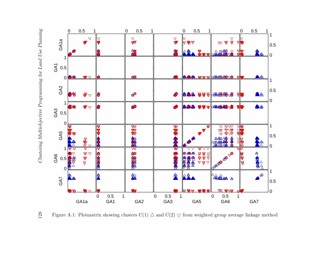
128
Clu
ster
ing
Mult
iobje
ctiv
eP
rogra
mm
ing
for
Land
Use
Pla
nnin
g
0
0.5
1
GA70 0.5 1
GA6
GA50 0.5 1
GA3
GA20 0.5 1
GA1
GA1a
GA
7
0
0.5
1
GA
6
0
0.5
1
GA
5
0
0.5
1
GA
3
0
0.5
1
GA
2
0
0.5
1G
A1
0 0.5 1
0
0.5
10 0.5 10 0.5 10 0.5 1
GA
1a
Figure A.1: Plotmatrix showing clusters C(1) 4 and C(2) 5 from weighted group average linkage method
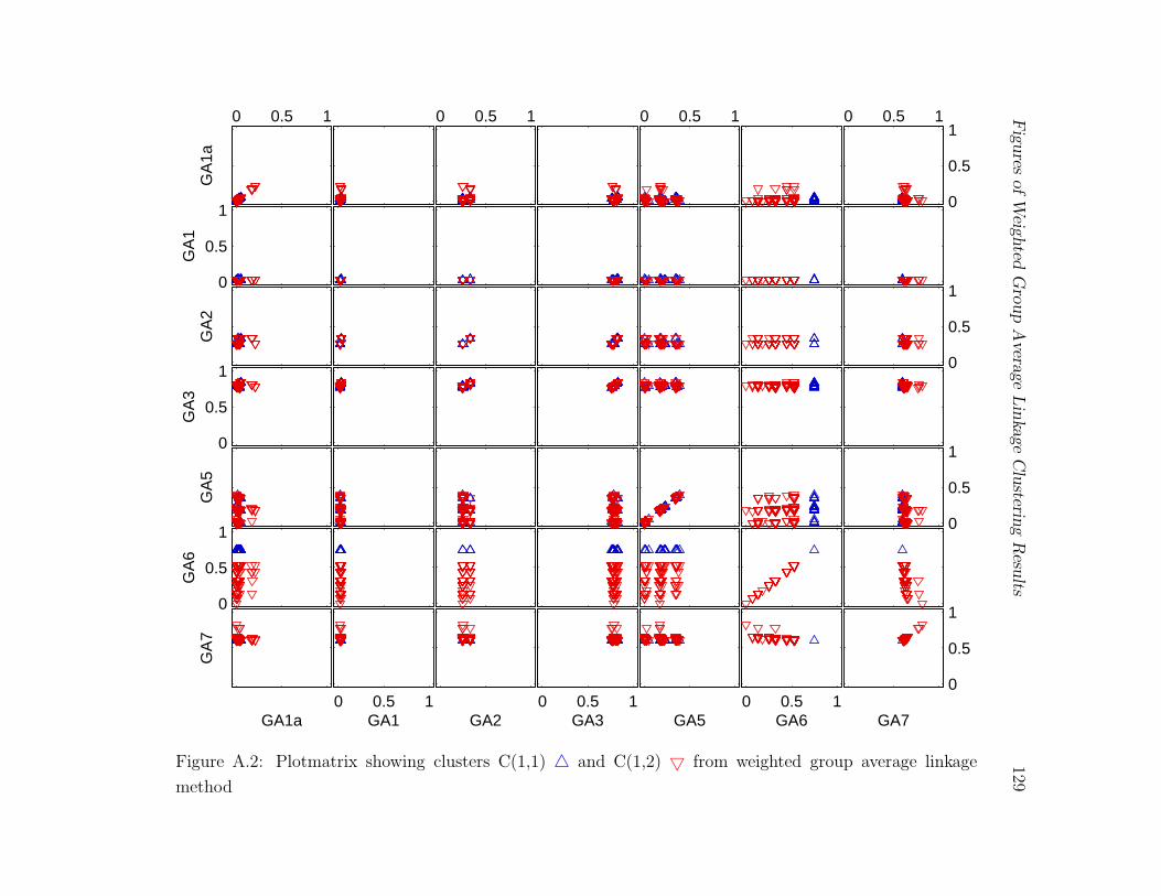
Fig
ures
ofW
eighted
Gro
up
Avera
ge
Lin
kage
Clu
stering
Resu
lts129
0
0.5
1
GA70 0.5 1
GA6
GA50 0.5 1
GA3
GA20 0.5 1
GA1
GA1a
GA
7
0
0.5
1
GA
6
0
0.5
1
GA
5
0
0.5
1
GA
3
0
0.5
1
GA
2
0
0.5
1G
A1
0 0.5 1
0
0.5
10 0.5 10 0.5 10 0.5 1
GA
1a
Figure A.2: Plotmatrix showing clusters C(1,1) 4 and C(1,2) 5 from weighted group average linkage
method
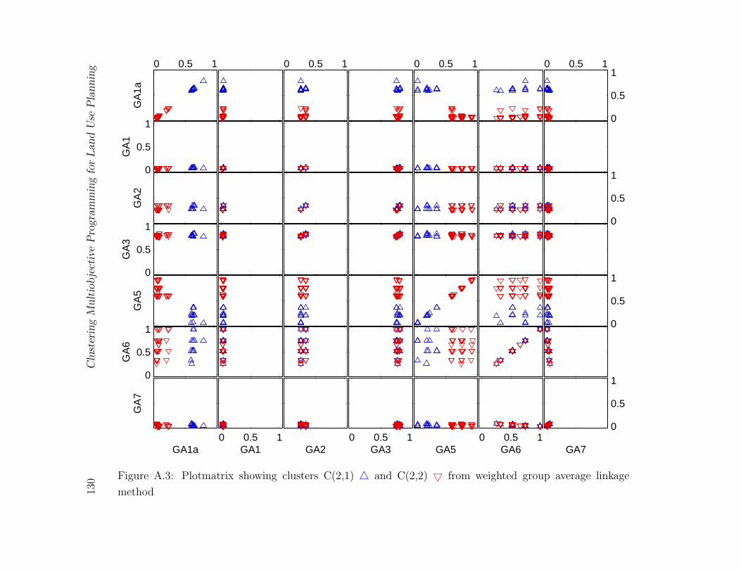
130
Clu
ster
ing
Mult
iobje
ctiv
eP
rogra
mm
ing
for
Land
Use
Pla
nnin
g
0
0.5
1
GA70 0.5 1
GA6
GA50 0.5 1
GA3
GA20 0.5 1
GA1
GA1a
GA
7
0
0.5
1
GA
6
0
0.5
1
GA
5
0
0.5
1
GA
3
0
0.5
1
GA
2
0
0.5
1G
A1
0 0.5 1
0
0.5
10 0.5 10 0.5 10 0.5 1
GA
1a
Figure A.3: Plotmatrix showing clusters C(2,1) 4 and C(2,2) 5 from weighted group average linkage
method
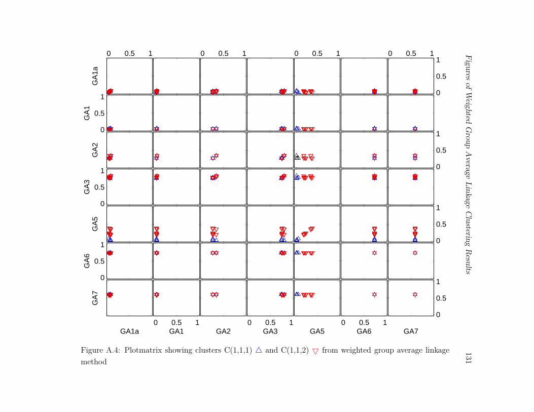
Fig
ures
ofW
eighted
Gro
up
Avera
ge
Lin
kage
Clu
stering
Resu
lts131
0
0.5
1
GA70 0.5 1
GA6
GA50 0.5 1
GA3
GA20 0.5 1
GA1
GA1a
GA
7
0
0.5
1
GA
6
0
0.5
1
GA
5
0
0.5
1
GA
3
0
0.5
1
GA
2
0
0.5
1G
A1
0 0.5 1
0
0.5
10 0.5 10 0.5 10 0.5 1
GA
1a
Figure A.4: Plotmatrix showing clusters C(1,1,1) 4 and C(1,1,2) 5 from weighted group average linkage
method
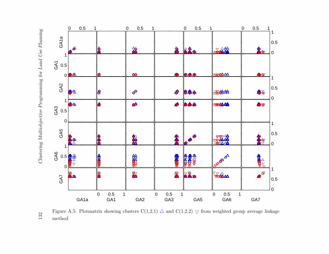
132
Clu
ster
ing
Mult
iobje
ctiv
eP
rogra
mm
ing
for
Land
Use
Pla
nnin
g
0
0.5
1
GA70 0.5 1
GA6
GA50 0.5 1
GA3
GA20 0.5 1
GA1
GA1a
GA
7
0
0.5
1
GA
6
0
0.5
1
GA
5
0
0.5
1
GA
3
0
0.5
1
GA
2
0
0.5
1G
A1
0 0.5 1
0
0.5
10 0.5 10 0.5 10 0.5 1
GA
1a
Figure A.5: Plotmatrix showing clusters C(1,2,1) 4 and C(1,2,2) 5 from weighted group average linkage
method
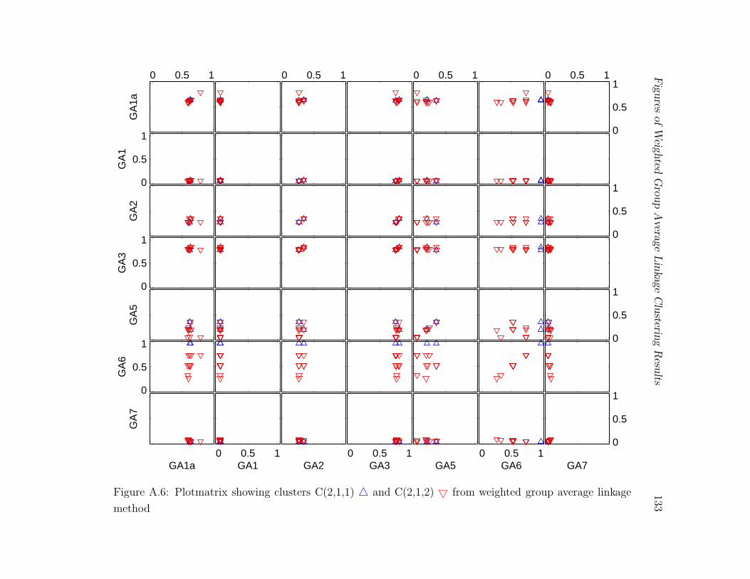
Fig
ures
ofW
eighted
Gro
up
Avera
ge
Lin
kage
Clu
stering
Resu
lts133
0
0.5
1
GA70 0.5 1
GA6
GA50 0.5 1
GA3
GA20 0.5 1
GA1
GA1a
GA
7
0
0.5
1
GA
6
0
0.5
1
GA
5
0
0.5
1
GA
3
0
0.5
1
GA
2
0
0.5
1G
A1
0 0.5 1
0
0.5
10 0.5 10 0.5 10 0.5 1
GA
1a
Figure A.6: Plotmatrix showing clusters C(2,1,1) 4 and C(2,1,2) 5 from weighted group average linkage
method
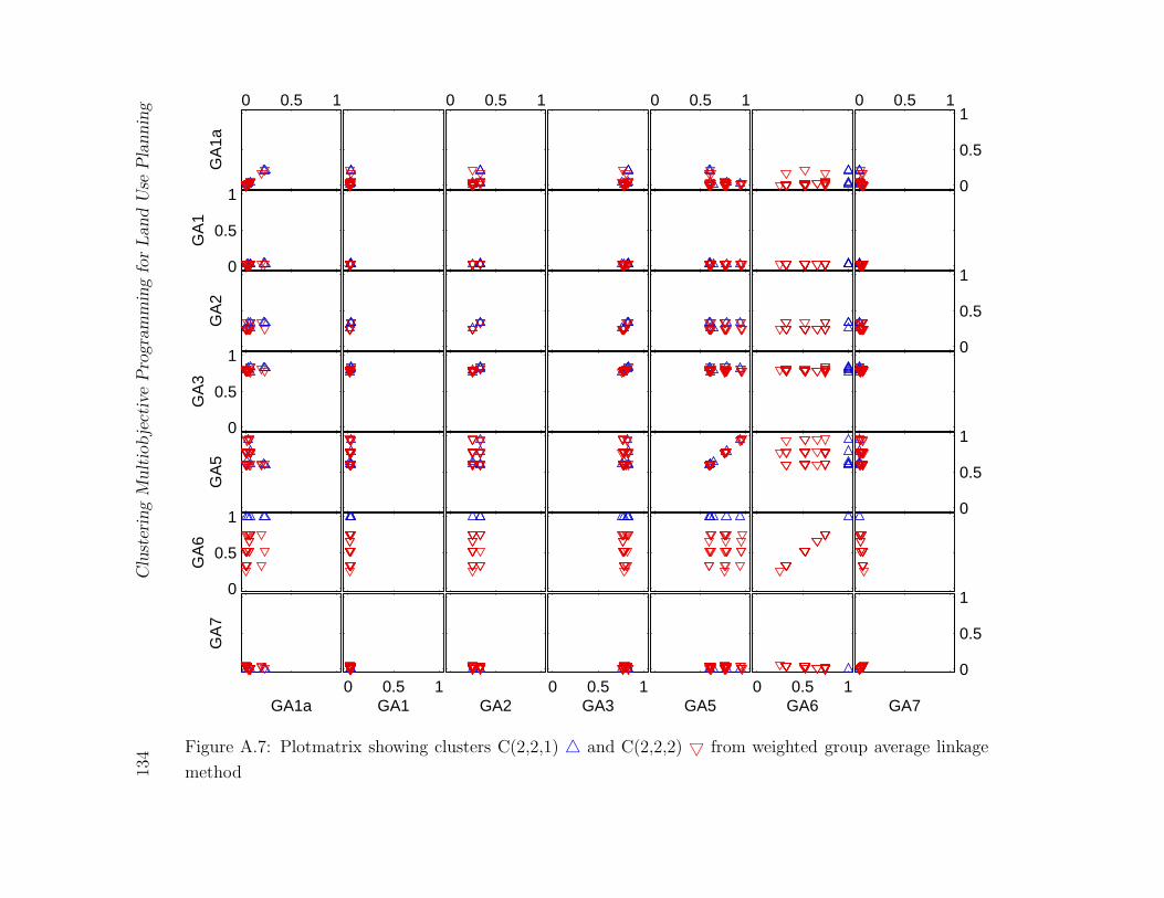
134
Clu
ster
ing
Mult
iobje
ctiv
eP
rogra
mm
ing
for
Land
Use
Pla
nnin
g
0
0.5
1
GA70 0.5 1
GA6
GA50 0.5 1
GA3
GA20 0.5 1
GA1
GA1a
GA
7
0
0.5
1
GA
6
0
0.5
1
GA
5
0
0.5
1
GA
3
0
0.5
1
GA
2
0
0.5
1G
A1
0 0.5 1
0
0.5
10 0.5 10 0.5 10 0.5 1
GA
1a
Figure A.7: Plotmatrix showing clusters C(2,2,1) 4 and C(2,2,2) 5 from weighted group average linkage
method
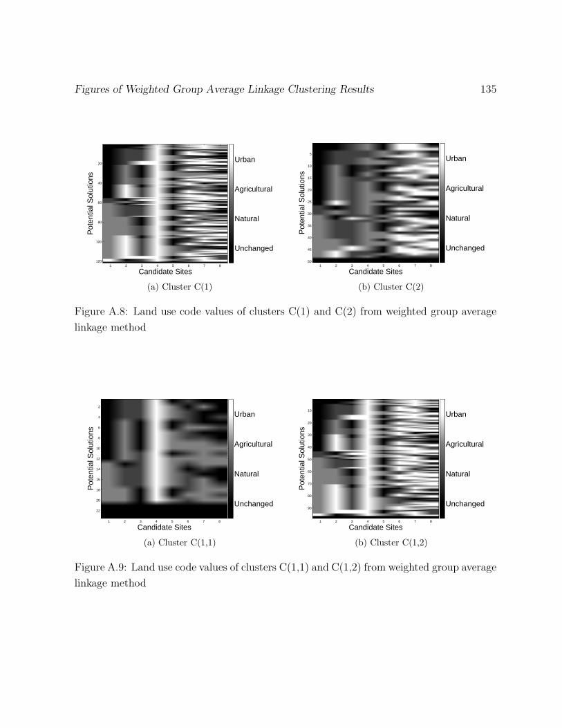
Figures of Weighted Group Average Linkage Clustering Results 135
Candidate Sites
Pot
entia
l Sol
utio
ns
1 2 3 4 5 6 7 8
20
40
60
80
100
120
Unchanged
Natural
Agricultural
Urban
(a) Cluster C(1)
Candidate Sites
Pot
entia
l Sol
utio
ns
1 2 3 4 5 6 7 8
5
10
15
20
25
30
35
40
45
50
Unchanged
Natural
Agricultural
Urban
(b) Cluster C(2)
Figure A.8: Land use code values of clusters C(1) and C(2) from weighted group average
linkage method
Candidate Sites
Pot
entia
l Sol
utio
ns
1 2 3 4 5 6 7 8
2
4
6
8
10
12
14
16
18
20
22
Unchanged
Natural
Agricultural
Urban
(a) Cluster C(1,1)
Candidate Sites
Pot
entia
l Sol
utio
ns
1 2 3 4 5 6 7 8
10
20
30
40
50
60
70
80
90Unchanged
Natural
Agricultural
Urban
(b) Cluster C(1,2)
Figure A.9: Land use code values of clusters C(1,1) and C(1,2) from weighted group average
linkage method
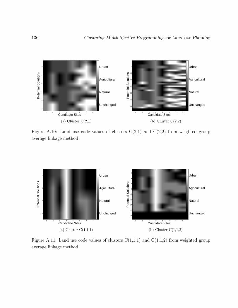
136 Clustering Multiobjective Programming for Land Use Planning
Candidate Sites
Pot
entia
l Sol
utio
ns
1 2 3 4 5 6 7 8
2
4
6
8
10
12
Unchanged
Natural
Agricultural
Urban
(a) Cluster C(2,1)
Candidate Sites
Pot
entia
l Sol
utio
ns
1 2 3 4 5 6 7 8
5
10
15
20
25
30
35Unchanged
Natural
Agricultural
Urban
(b) Cluster C(2,2)
Figure A.10: Land use code values of clusters C(2,1) and C(2,2) from weighted group
average linkage method
Candidate Sites
Pot
entia
l Sol
utio
ns
1 2 3 4 5 6 7 8
1
2
3
4 Unchanged
Natural
Agricultural
Urban
(a) Cluster C(1,1,1)
Candidate Sites
Pot
entia
l Sol
utio
ns
1 2 3 4 5 6 7 8
2
4
6
8
10
12
14
16
18Unchanged
Natural
Agricultural
Urban
(b) Cluster C(1,1,2)
Figure A.11: Land use code values of clusters C(1,1,1) and C(1,1,2) from weighted group
average linkage method
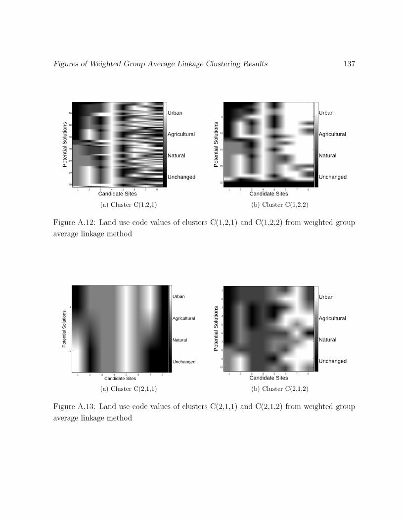
Figures of Weighted Group Average Linkage Clustering Results 137
Candidate Sites
Pot
entia
l Sol
utio
ns
1 2 3 4 5 6 7 8
10
20
30
40
50
60
70
Unchanged
Natural
Agricultural
Urban
(a) Cluster C(1,2,1)
Candidate Sites
Pot
entia
l Sol
utio
ns
1 2 3 4 5 6 7 8
5
10
15
20
25
Unchanged
Natural
Agricultural
Urban
(b) Cluster C(1,2,2)
Figure A.12: Land use code values of clusters C(1,2,1) and C(1,2,2) from weighted group
average linkage method
Candidate Sites
Pot
entia
l Sol
utio
ns
1 2 3 4 5 6 7 8
1
2
Unchanged
Natural
Agricultural
Urban
(a) Cluster C(2,1,1)
Candidate Sites
Pot
entia
l Sol
utio
ns
1 2 3 4 5 6 7 8
1
2
3
4
5
6
7
8
9
10
Unchanged
Natural
Agricultural
Urban
(b) Cluster C(2,1,2)
Figure A.13: Land use code values of clusters C(2,1,1) and C(2,1,2) from weighted group
average linkage method
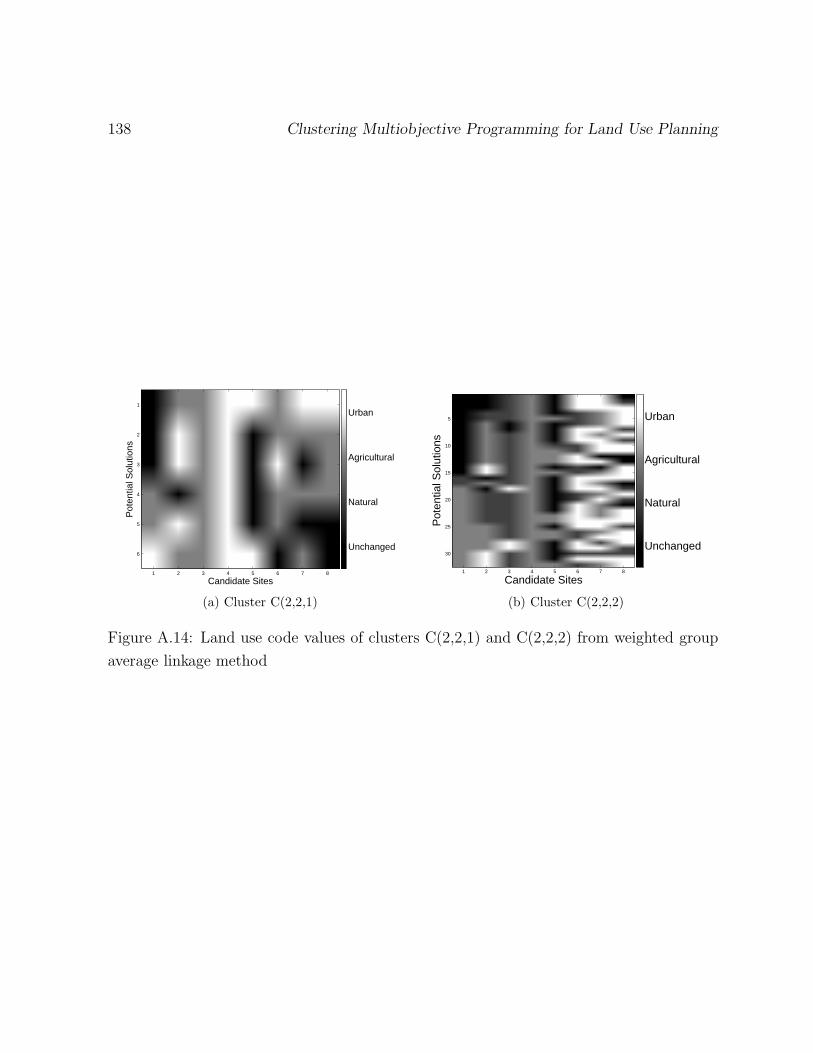
138 Clustering Multiobjective Programming for Land Use Planning
Candidate Sites
Pot
entia
l Sol
utio
ns
1 2 3 4 5 6 7 8
1
2
3
4
5
6Unchanged
Natural
Agricultural
Urban
(a) Cluster C(2,2,1)
Candidate Sites
Pot
entia
l Sol
utio
ns
1 2 3 4 5 6 7 8
5
10
15
20
25
30Unchanged
Natural
Agricultural
Urban
(b) Cluster C(2,2,2)
Figure A.14: Land use code values of clusters C(2,2,1) and C(2,2,2) from weighted group
average linkage method
Appendix B
Figures of Complete Linkage
Clustering Results
139
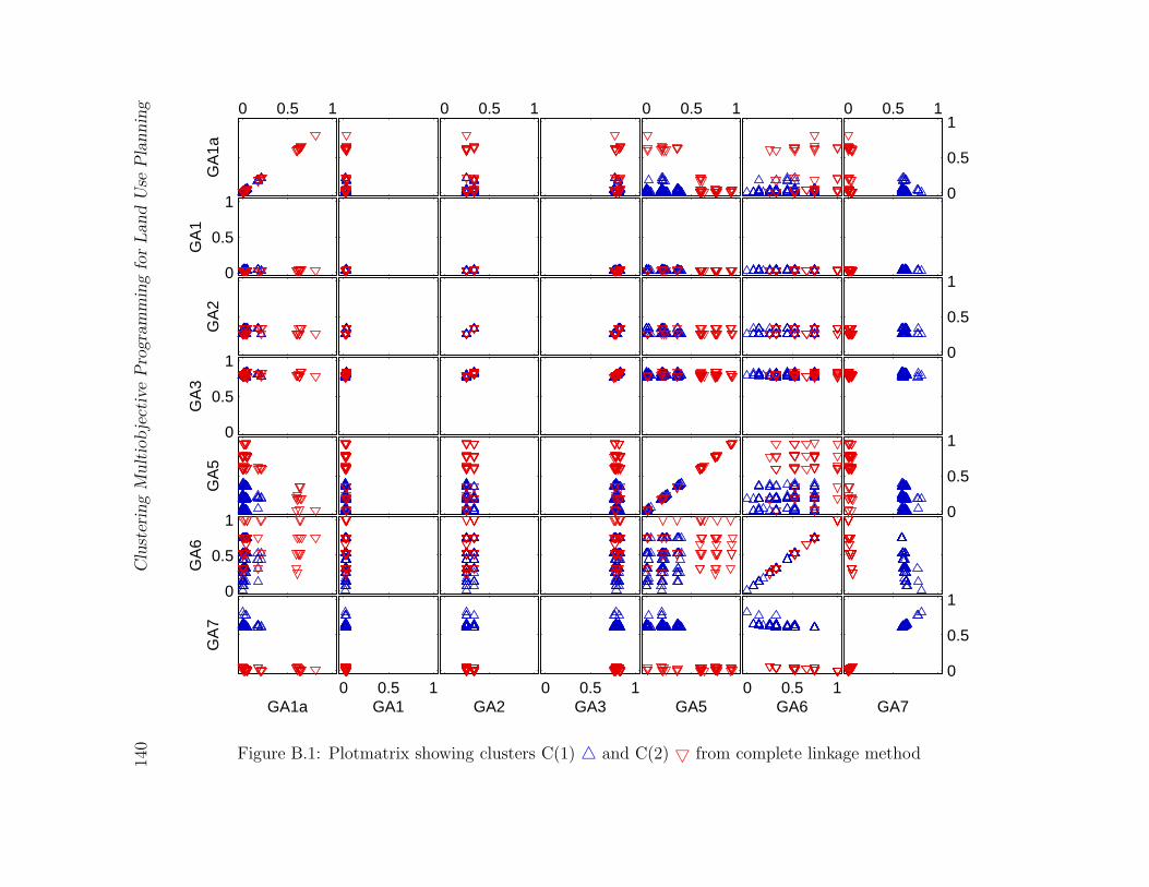
140
Clu
ster
ing
Mult
iobje
ctiv
eP
rogra
mm
ing
for
Land
Use
Pla
nnin
g
0
0.5
1
GA70 0.5 1
GA6
GA50 0.5 1
GA3
GA20 0.5 1
GA1
GA1a
GA
7
0
0.5
1
GA
6
0
0.5
1
GA
5
0
0.5
1
GA
3
0
0.5
1
GA
2
0
0.5
1G
A1
0 0.5 1
0
0.5
10 0.5 10 0.5 10 0.5 1
GA
1a
Figure B.1: Plotmatrix showing clusters C(1) 4 and C(2) 5 from complete linkage method
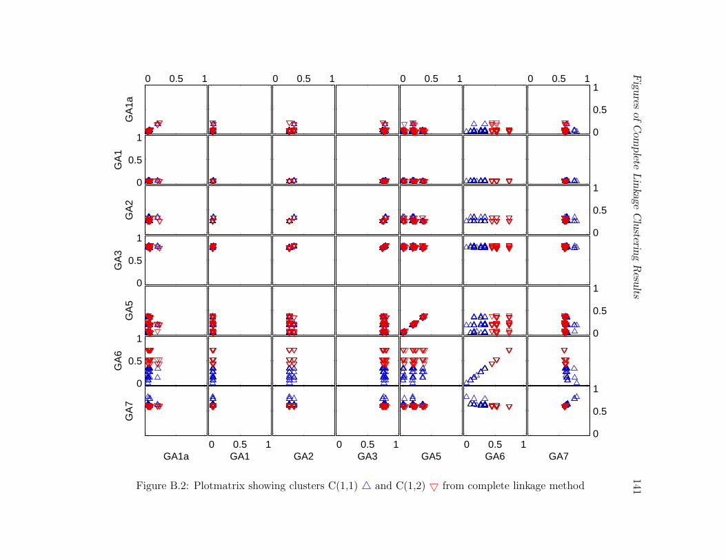
Fig
ures
ofC
om
plete
Lin
kage
Clu
stering
Resu
lts141
0
0.5
1
GA70 0.5 1
GA6
GA50 0.5 1
GA3
GA20 0.5 1
GA1
GA1a
GA
7
0
0.5
1
GA
6
0
0.5
1
GA
5
0
0.5
1
GA
3
0
0.5
1
GA
2
0
0.5
1
GA
1
0 0.5 1
0
0.5
10 0.5 10 0.5 10 0.5 1
GA
1a
Figure B.2: Plotmatrix showing clusters C(1,1) 4 and C(1,2) 5 from complete linkage method
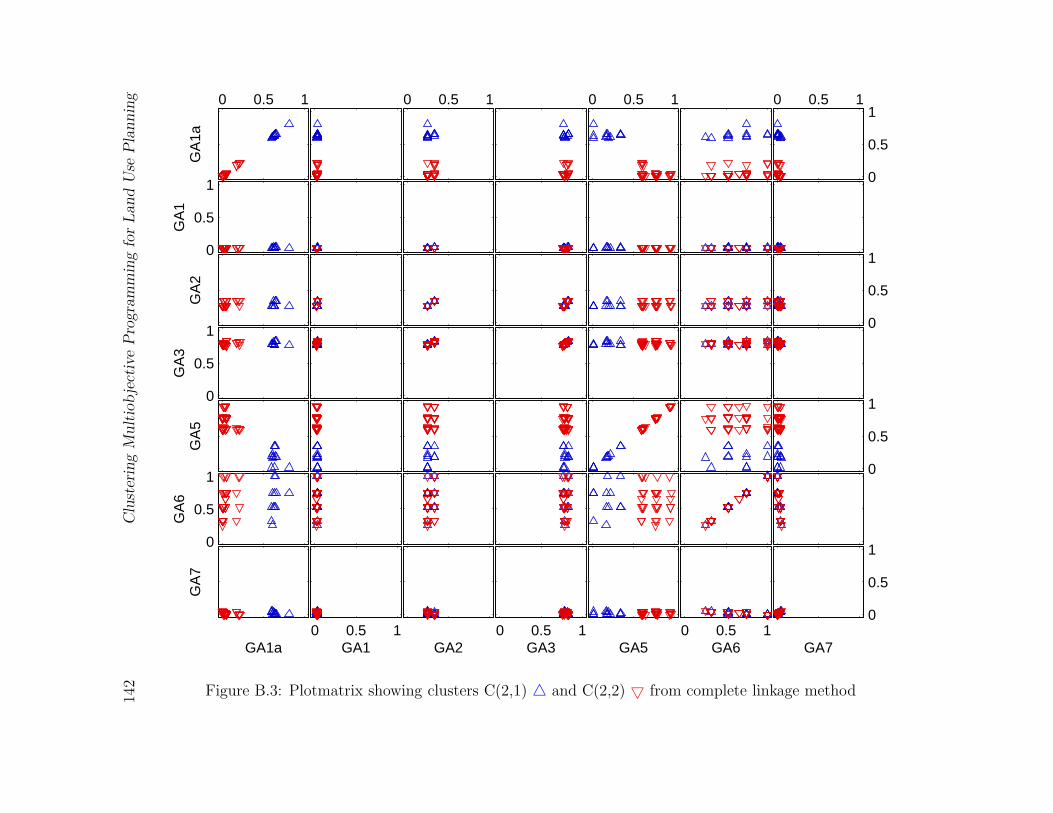
142
Clu
ster
ing
Mult
iobje
ctiv
eP
rogra
mm
ing
for
Land
Use
Pla
nnin
g
0
0.5
1
GA70 0.5 1
GA6
GA50 0.5 1
GA3
GA20 0.5 1
GA1
GA1a
GA
7
0
0.5
1
GA
6
0
0.5
1
GA
5
0
0.5
1
GA
3
0
0.5
1
GA
2
0
0.5
1G
A1
0 0.5 1
0
0.5
10 0.5 10 0.5 10 0.5 1
GA
1a
Figure B.3: Plotmatrix showing clusters C(2,1) 4 and C(2,2) 5 from complete linkage method
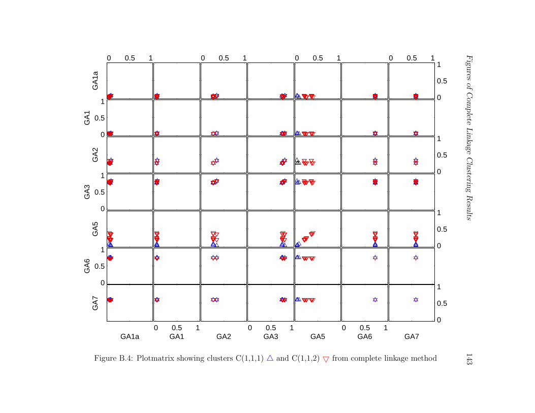
Fig
ures
ofC
om
plete
Lin
kage
Clu
stering
Resu
lts143
0
0.5
1
GA70 0.5 1
GA6
GA50 0.5 1
GA3
GA20 0.5 1
GA1
GA1a
GA
7
0
0.5
1
GA
6
0
0.5
1
GA
5
0
0.5
1
GA
3
0
0.5
1
GA
2
0
0.5
1
GA
1
0 0.5 1
0
0.5
10 0.5 10 0.5 10 0.5 1
GA
1a
Figure B.4: Plotmatrix showing clusters C(1,1,1) 4 and C(1,1,2) 5 from complete linkage method
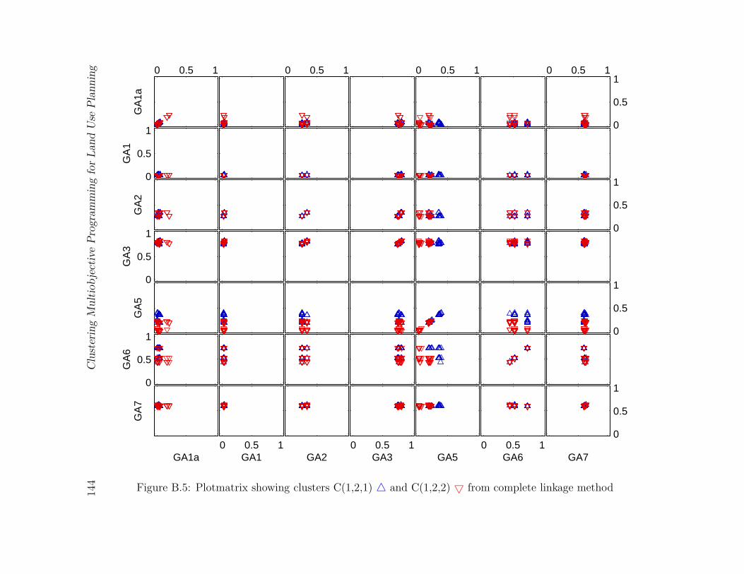
144
Clu
ster
ing
Mult
iobje
ctiv
eP
rogra
mm
ing
for
Land
Use
Pla
nnin
g
0
0.5
1
GA70 0.5 1
GA6
GA50 0.5 1
GA3
GA20 0.5 1
GA1
GA1a
GA
7
0
0.5
1
GA
6
0
0.5
1
GA
5
0
0.5
1
GA
3
0
0.5
1
GA
2
0
0.5
1G
A1
0 0.5 1
0
0.5
10 0.5 10 0.5 10 0.5 1
GA
1a
Figure B.5: Plotmatrix showing clusters C(1,2,1) 4 and C(1,2,2) 5 from complete linkage method
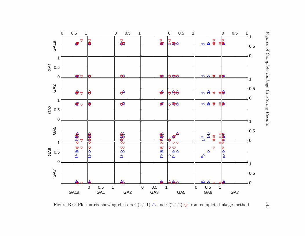
Fig
ures
ofC
om
plete
Lin
kage
Clu
stering
Resu
lts145
0
0.5
1
GA70 0.5 1
GA6
GA50 0.5 1
GA3
GA20 0.5 1
GA1
GA1a
GA
7
0
0.5
1
GA
6
0
0.5
1
GA
5
0
0.5
1
GA
3
0
0.5
1
GA
2
0
0.5
1
GA
1
0 0.5 1
0
0.5
10 0.5 10 0.5 10 0.5 1
GA
1a
Figure B.6: Plotmatrix showing clusters C(2,1,1) 4 and C(2,1,2) 5 from complete linkage method
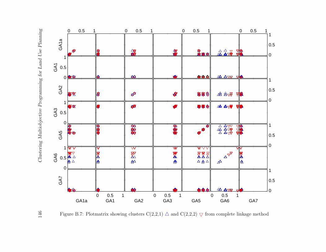
146
Clu
ster
ing
Mult
iobje
ctiv
eP
rogra
mm
ing
for
Land
Use
Pla
nnin
g
0
0.5
1
GA70 0.5 1
GA6
GA50 0.5 1
GA3
GA20 0.5 1
GA1
GA1a
GA
7
0
0.5
1
GA
6
0
0.5
1
GA
5
0
0.5
1
GA
3
0
0.5
1
GA
2
0
0.5
1G
A1
0 0.5 1
0
0.5
10 0.5 10 0.5 10 0.5 1
GA
1a
Figure B.7: Plotmatrix showing clusters C(2,2,1) 4 and C(2,2,2) 5 from complete linkage method

Appendix C
Figures of Chameleon Results
147
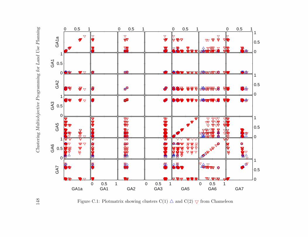
148
Clu
ster
ing
Mult
iobje
ctiv
eP
rogra
mm
ing
for
Land
Use
Pla
nnin
g
0
0.5
1
GA70 0.5 1
GA6
GA50 0.5 1
GA3
GA20 0.5 1
GA1
GA1a
GA
7
0
0.5
1
GA
6
0
0.5
1
GA
5
0
0.5
1
GA
3
0
0.5
1
GA
2
0
0.5
1G
A1
0 0.5 1
0
0.5
10 0.5 10 0.5 10 0.5 1
GA
1a
Figure C.1: Plotmatrix showing clusters C(1) 4 and C(2) 5 from Chameleon
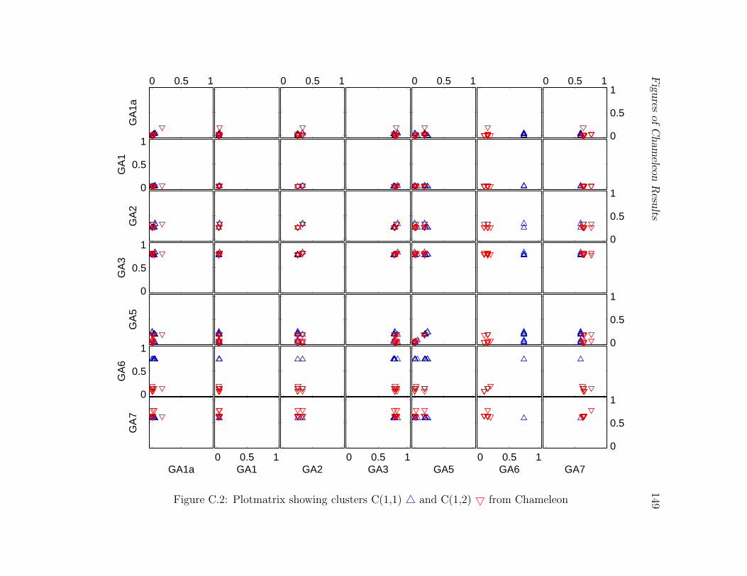
Fig
ures
ofC
ham
eleon
Resu
lts149
0
0.5
1
GA70 0.5 1
GA6
GA50 0.5 1
GA3
GA20 0.5 1
GA1
GA1a
GA
7
0
0.5
1
GA
6
0
0.5
1
GA
5
0
0.5
1
GA
3
0
0.5
1
GA
2
0
0.5
1
GA
1
0 0.5 1
0
0.5
10 0.5 10 0.5 10 0.5 1
GA
1a
Figure C.2: Plotmatrix showing clusters C(1,1) 4 and C(1,2) 5 from Chameleon
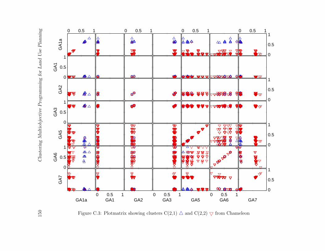
150
Clu
ster
ing
Mult
iobje
ctiv
eP
rogra
mm
ing
for
Land
Use
Pla
nnin
g
0
0.5
1
GA70 0.5 1
GA6
GA50 0.5 1
GA3
GA20 0.5 1
GA1
GA1a
GA
7
0
0.5
1
GA
6
0
0.5
1
GA
5
0
0.5
1
GA
3
0
0.5
1
GA
2
0
0.5
1G
A1
0 0.5 1
0
0.5
10 0.5 10 0.5 10 0.5 1
GA
1a
Figure C.3: Plotmatrix showing clusters C(2,1) 4 and C(2,2) 5 from Chameleon
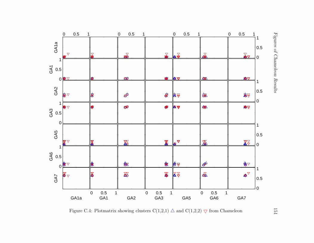
Fig
ures
ofC
ham
eleon
Resu
lts151
0
0.5
1
GA70 0.5 1
GA6
GA50 0.5 1
GA3
GA20 0.5 1
GA1
GA1a
GA
7
0
0.5
1
GA
6
0
0.5
1
GA
5
0
0.5
1
GA
3
0
0.5
1
GA
2
0
0.5
1
GA
1
0 0.5 1
0
0.5
10 0.5 10 0.5 10 0.5 1
GA
1a
Figure C.4: Plotmatrix showing clusters C(1,2,1) 4 and C(1,2,2) 5 from Chameleon
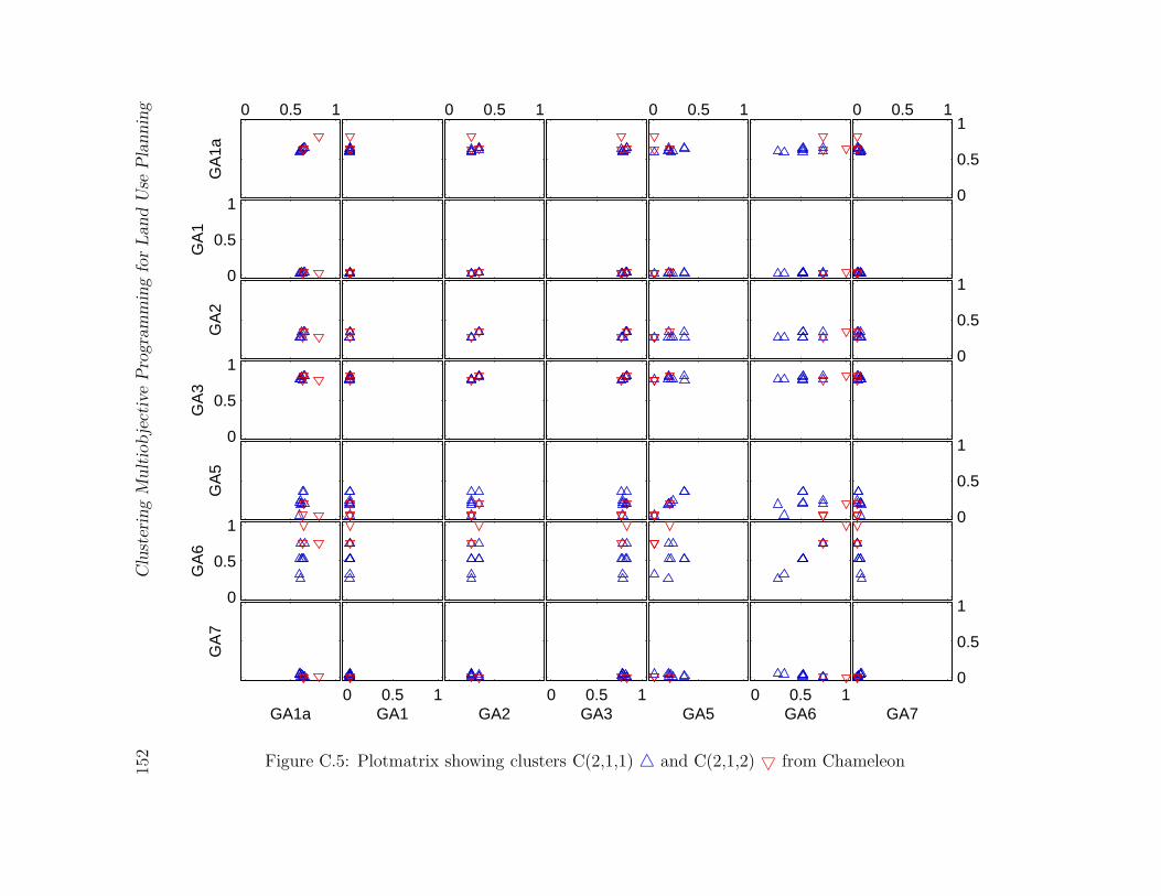
152
Clu
ster
ing
Mult
iobje
ctiv
eP
rogra
mm
ing
for
Land
Use
Pla
nnin
g
0
0.5
1
GA70 0.5 1
GA6
GA50 0.5 1
GA3
GA20 0.5 1
GA1
GA1a
GA
7
0
0.5
1
GA
6
0
0.5
1
GA
5
0
0.5
1
GA
3
0
0.5
1
GA
2
0
0.5
1G
A1
0 0.5 1
0
0.5
10 0.5 10 0.5 10 0.5 1
GA
1a
Figure C.5: Plotmatrix showing clusters C(2,1,1) 4 and C(2,1,2) 5 from Chameleon
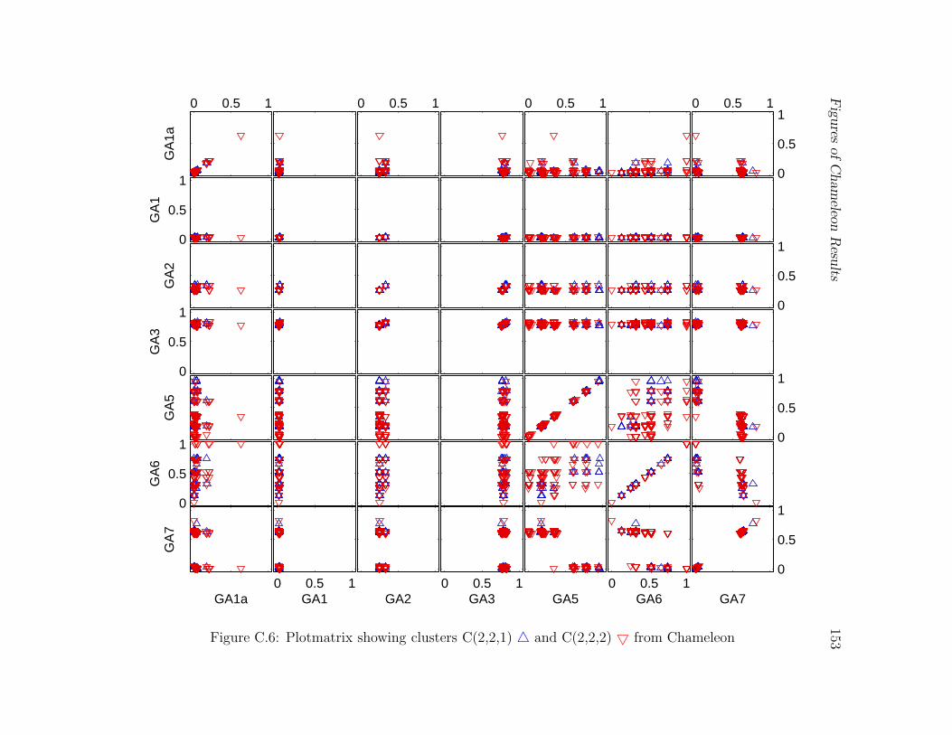
Fig
ures
ofC
ham
eleon
Resu
lts153
0
0.5
1
GA70 0.5 1
GA6
GA50 0.5 1
GA3
GA20 0.5 1
GA1
GA1a
GA
7
0
0.5
1
GA
6
0
0.5
1
GA
5
0
0.5
1
GA
3
0
0.5
1
GA
2
0
0.5
1
GA
1
0 0.5 1
0
0.5
10 0.5 10 0.5 10 0.5 1
GA
1a
Figure C.6: Plotmatrix showing clusters C(2,2,1) 4 and C(2,2,2) 5 from Chameleon


Appendix D
Figures of DBSCAN Results
155
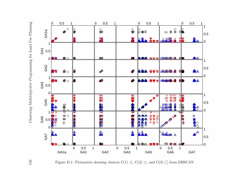
156
Clu
ster
ing
Mult
iobje
ctiv
eP
rogra
mm
ing
for
Land
Use
Pla
nnin
g
0
0.5
1
GA70 0.5 1
GA6
GA50 0.5 1
GA3
GA20 0.5 1
GA1
GA1a
GA
7
0
0.5
1
GA
6
0
0.5
1
GA
5
0
0.5
1
GA
3
0
0.5
1
GA
2
0
0.5
1G
A1
0 0.5 1
0
0.5
10 0.5 10 0.5 10 0.5 1
GA
1a
Figure D.1: Plotmatrix showing clusters C(1) 4, C(2) 5, and C(3) © from DBSCAN
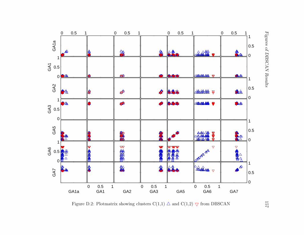
Fig
ures
ofD
BSC
AN
Resu
lts157
0
0.5
1
GA70 0.5 1
GA6
GA50 0.5 1
GA3
GA20 0.5 1
GA1
GA1a
GA
7
0
0.5
1
GA
6
0
0.5
1
GA
5
0
0.5
1
GA
3
0
0.5
1
GA
2
0
0.5
1
GA
1
0 0.5 1
0
0.5
10 0.5 10 0.5 10 0.5 1
GA
1a
Figure D.2: Plotmatrix showing clusters C(1,1) 4 and C(1,2) 5 from DBSCAN
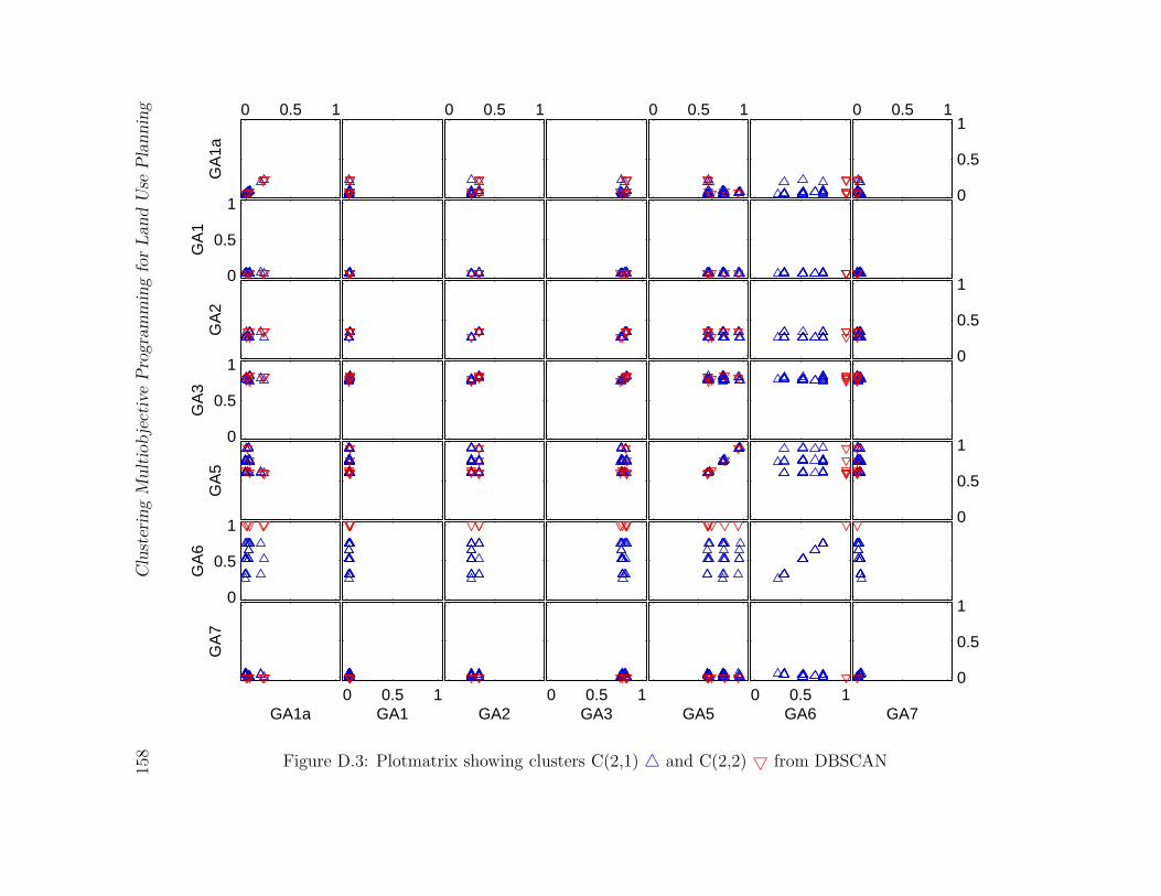
158
Clu
ster
ing
Mult
iobje
ctiv
eP
rogra
mm
ing
for
Land
Use
Pla
nnin
g
0
0.5
1
GA70 0.5 1
GA6
GA50 0.5 1
GA3
GA20 0.5 1
GA1
GA1a
GA
7
0
0.5
1
GA
6
0
0.5
1
GA
5
0
0.5
1
GA
3
0
0.5
1
GA
2
0
0.5
1G
A1
0 0.5 1
0
0.5
10 0.5 10 0.5 10 0.5 1
GA
1a
Figure D.3: Plotmatrix showing clusters C(2,1) 4 and C(2,2) 5 from DBSCAN
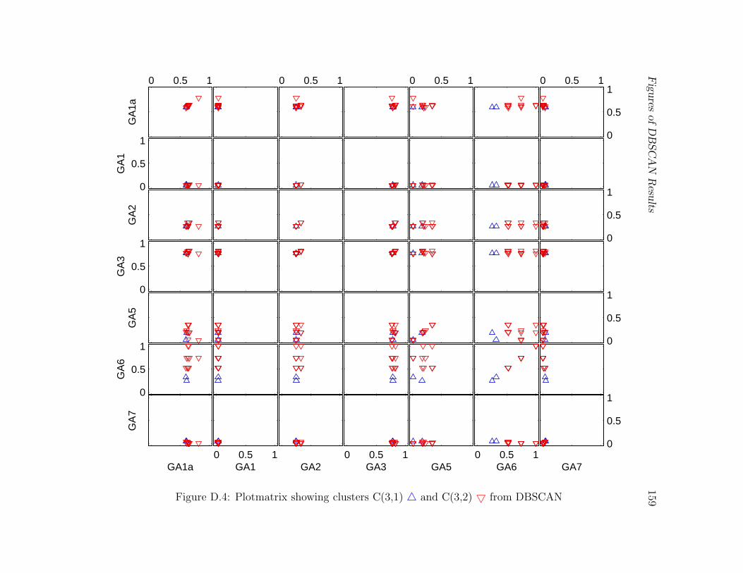
Fig
ures
ofD
BSC
AN
Resu
lts159
0
0.5
1
GA70 0.5 1
GA6
GA50 0.5 1
GA3
GA20 0.5 1
GA1
GA1a
GA
7
0
0.5
1
GA
6
0
0.5
1
GA
5
0
0.5
1
GA
3
0
0.5
1
GA
2
0
0.5
1
GA
1
0 0.5 1
0
0.5
10 0.5 10 0.5 10 0.5 1
GA
1a
Figure D.4: Plotmatrix showing clusters C(3,1) 4 and C(3,2) 5 from DBSCAN
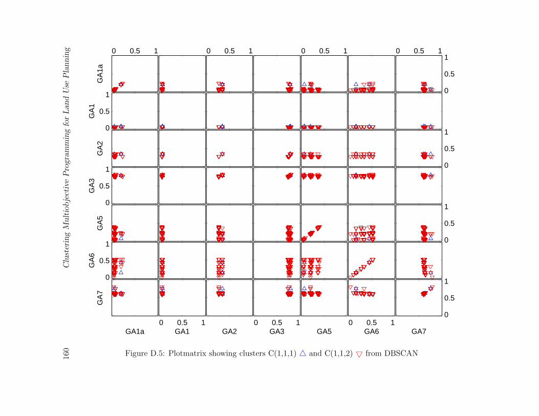
160
Clu
ster
ing
Mult
iobje
ctiv
eP
rogra
mm
ing
for
Land
Use
Pla
nnin
g
0
0.5
1
GA70 0.5 1
GA6
GA50 0.5 1
GA3
GA20 0.5 1
GA1
GA1a
GA
7
0
0.5
1
GA
6
0
0.5
1
GA
5
0
0.5
1
GA
3
0
0.5
1
GA
2
0
0.5
1G
A1
0 0.5 1
0
0.5
10 0.5 10 0.5 10 0.5 1
GA
1a
Figure D.5: Plotmatrix showing clusters C(1,1,1) 4 and C(1,1,2) 5 from DBSCAN
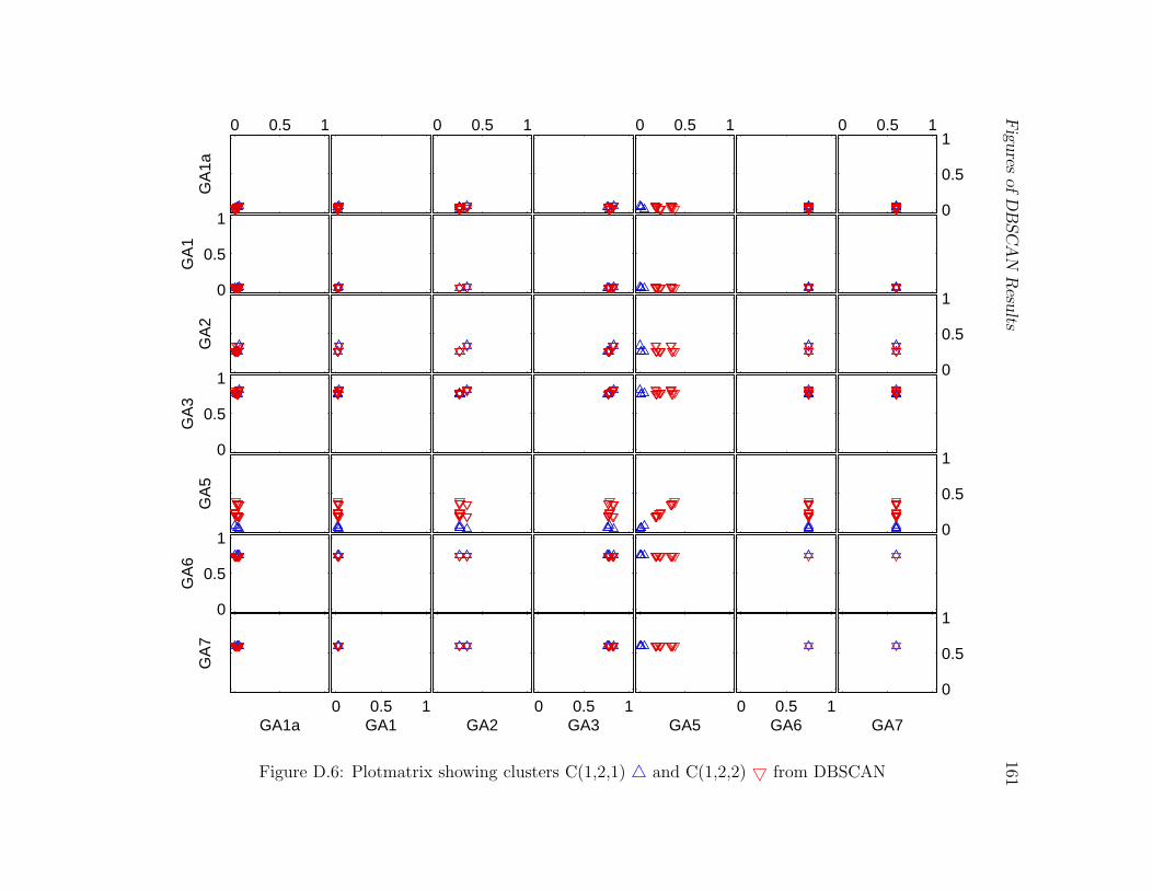
Fig
ures
ofD
BSC
AN
Resu
lts161
0
0.5
1
GA70 0.5 1
GA6
GA50 0.5 1
GA3
GA20 0.5 1
GA1
GA1a
GA
7
0
0.5
1
GA
6
0
0.5
1
GA
5
0
0.5
1
GA
3
0
0.5
1
GA
2
0
0.5
1
GA
1
0 0.5 1
0
0.5
10 0.5 10 0.5 10 0.5 1
GA
1a
Figure D.6: Plotmatrix showing clusters C(1,2,1) 4 and C(1,2,2) 5 from DBSCAN
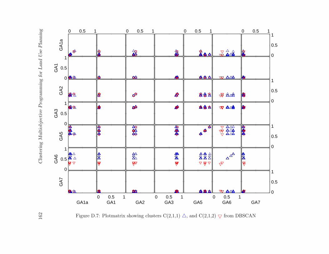
162
Clu
ster
ing
Mult
iobje
ctiv
eP
rogra
mm
ing
for
Land
Use
Pla
nnin
g
0
0.5
1
GA70 0.5 1
GA6
GA50 0.5 1
GA3
GA20 0.5 1
GA1
GA1a
GA
7
0
0.5
1
GA
6
0
0.5
1
GA
5
0
0.5
1
GA
3
0
0.5
1
GA
2
0
0.5
1G
A1
0 0.5 1
0
0.5
10 0.5 10 0.5 10 0.5 1
GA
1a
Figure D.7: Plotmatrix showing clusters C(2,1,1) 4, and C(2,1,2) 5 from DBSCAN
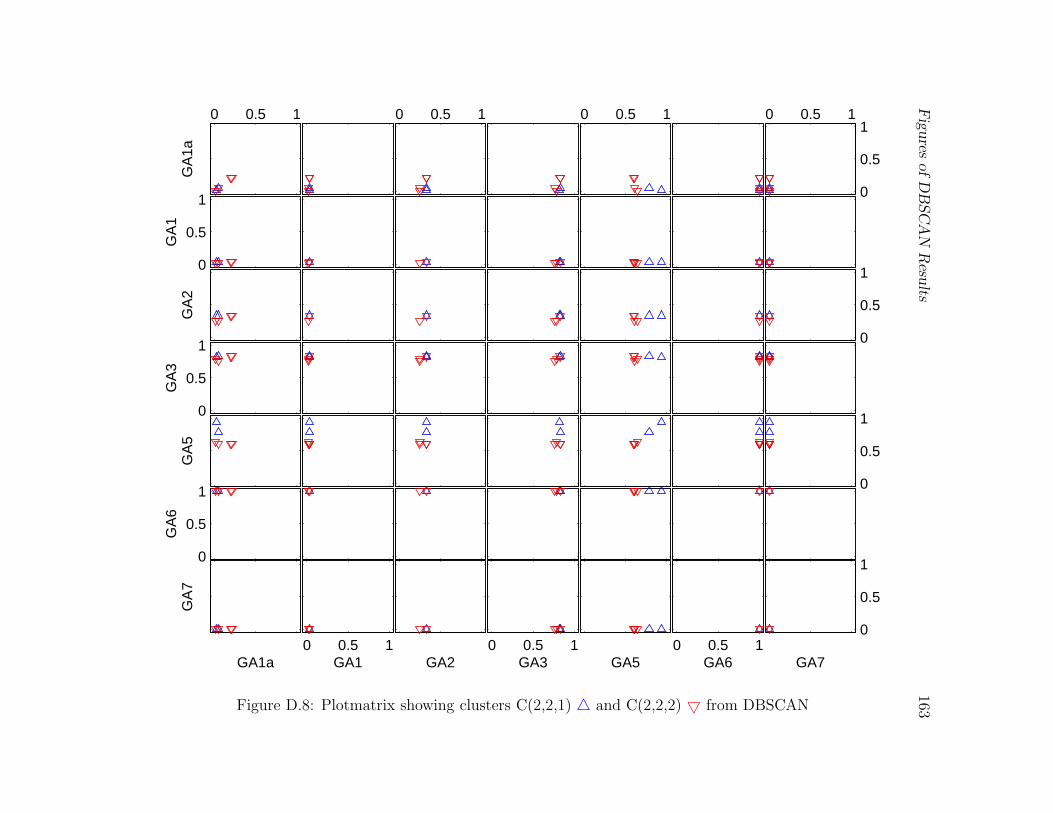
Fig
ures
ofD
BSC
AN
Resu
lts163
0
0.5
1
GA70 0.5 1
GA6
GA50 0.5 1
GA3
GA20 0.5 1
GA1
GA1a
GA
7
0
0.5
1
GA
6
0
0.5
1
GA
5
0
0.5
1
GA
3
0
0.5
1
GA
2
0
0.5
1
GA
1
0 0.5 1
0
0.5
10 0.5 10 0.5 10 0.5 1
GA
1a
Figure D.8: Plotmatrix showing clusters C(2,2,1) 4 and C(2,2,2) 5 from DBSCAN
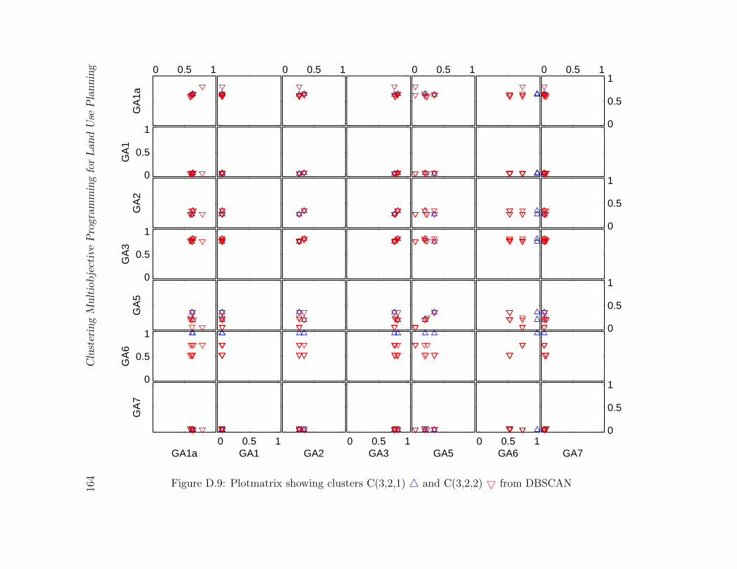
164
Clu
ster
ing
Mult
iobje
ctiv
eP
rogra
mm
ing
for
Land
Use
Pla
nnin
g
0
0.5
1
GA70 0.5 1
GA6
GA50 0.5 1
GA3
GA20 0.5 1
GA1
GA1a
GA
7
0
0.5
1
GA
6
0
0.5
1
GA
5
0
0.5
1
GA
3
0
0.5
1
GA
2
0
0.5
1G
A1
0 0.5 1
0
0.5
10 0.5 10 0.5 10 0.5 1
GA
1a
Figure D.9: Plotmatrix showing clusters C(3,2,1) 4 and C(3,2,2) 5 from DBSCAN

Appendix E
Figures of Unsupervised Decision
Tree Results
165
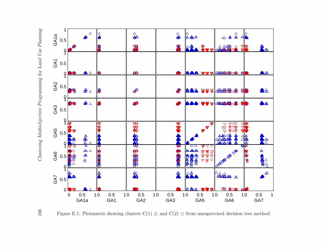
166
Clu
ster
ing
Mult
iobje
ctiv
eP
rogra
mm
ing
for
Land
Use
Pla
nnin
g
0 0.5 1GA7
0 0.5 1GA6
0 0.5 1GA5
0 0.5 1GA3
0 0.5 1GA2
0 0.5 1GA1
0 0.5 10
0.5
1
GA1a
GA
7
0
0.5
1
GA
6
0
0.5
1
GA
5
0
0.5
1
GA
3
0
0.5
1
GA
2
0
0.5
1G
A1
0
0.5
1
GA
1a
Figure E.1: Plotmatrix showing clusters C(1) 4 and C(2) 5 from unsupervised decision tree method
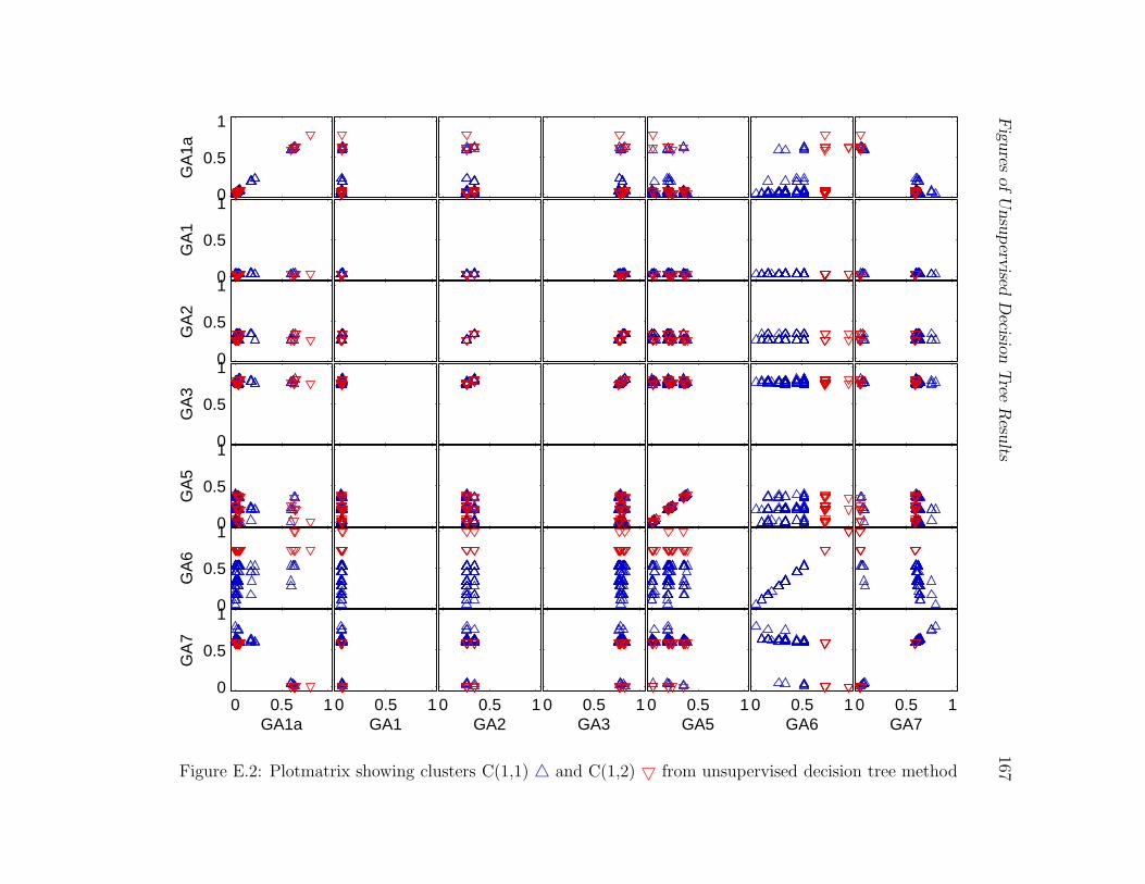
Fig
ures
ofU
nsu
perv
isedD
ecision
Tree
Resu
lts167
0 0.5 1GA7
0 0.5 1GA6
0 0.5 1GA5
0 0.5 1GA3
0 0.5 1GA2
0 0.5 1GA1
0 0.5 10
0.5
1
GA1a
GA
7
0
0.5
1
GA
6
0
0.5
1
GA
5
0
0.5
1
GA
3
0
0.5
1
GA
2
0
0.5
1G
A1
0
0.5
1
GA
1a
Figure E.2: Plotmatrix showing clusters C(1,1) 4 and C(1,2) 5 from unsupervised decision tree method
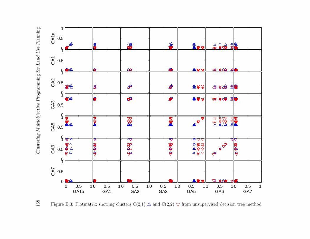
168
Clu
ster
ing
Mult
iobje
ctiv
eP
rogra
mm
ing
for
Land
Use
Pla
nnin
g
0 0.5 1GA7
0 0.5 1GA6
0 0.5 1GA5
0 0.5 1GA3
0 0.5 1GA2
0 0.5 1GA1
0 0.5 10
0.5
1
GA1a
GA
7
0
0.5
1
GA
6
0
0.5
1
GA
5
0
0.5
1
GA
3
0
0.5
1
GA
2
0
0.5
1G
A1
0
0.5
1
GA
1a
Figure E.3: Plotmatrix showing clusters C(2,1) 4 and C(2,2) 5 from unsupervised decision tree method
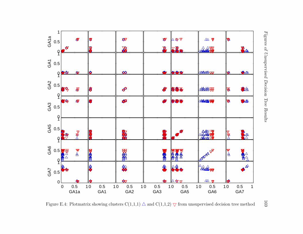
Fig
ures
ofU
nsu
perv
isedD
ecision
Tree
Resu
lts169
0 0.5 1GA7
0 0.5 1GA6
0 0.5 1GA5
0 0.5 1GA3
0 0.5 1GA2
0 0.5 1GA1
0 0.5 10
0.5
1
GA1a
GA
7
0
0.5
1
GA
6
0
0.5
1
GA
5
0
0.5
1
GA
3
0
0.5
1
GA
2
0
0.5
1G
A1
0
0.5
1
GA
1a
Figure E.4: Plotmatrix showing clusters C(1,1,1)4 and C(1,1,2)5 from unsupervised decision tree method
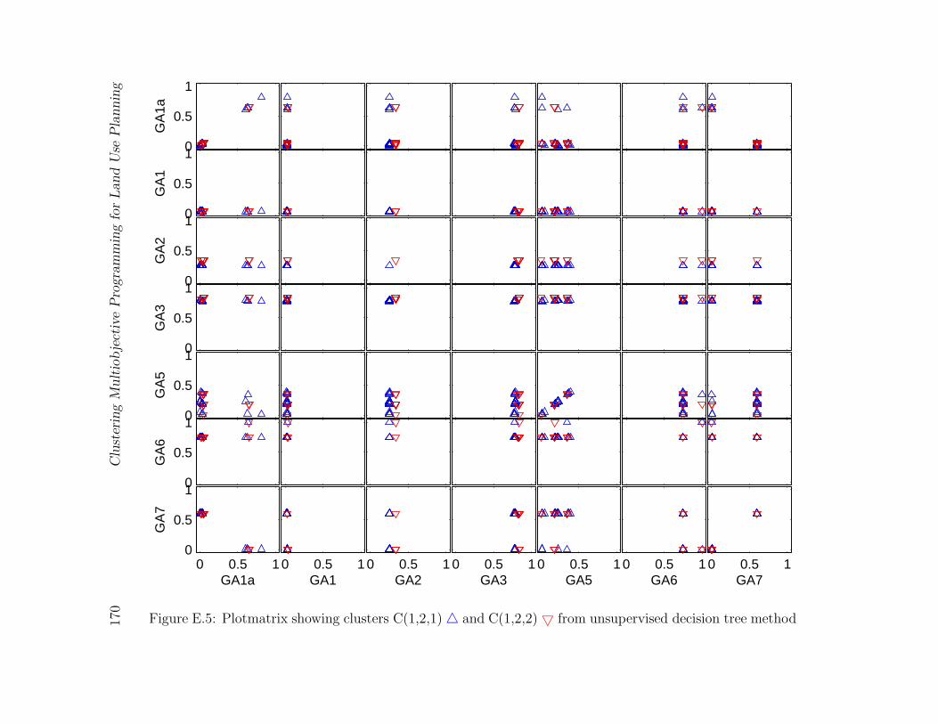
170
Clu
ster
ing
Mult
iobje
ctiv
eP
rogra
mm
ing
for
Land
Use
Pla
nnin
g
0 0.5 1GA7
0 0.5 1GA6
0 0.5 1GA5
0 0.5 1GA3
0 0.5 1GA2
0 0.5 1GA1
0 0.5 10
0.5
1
GA1a
GA
7
0
0.5
1
GA
6
0
0.5
1
GA
5
0
0.5
1
GA
3
0
0.5
1
GA
2
0
0.5
1G
A1
0
0.5
1
GA
1a
Figure E.5: Plotmatrix showing clusters C(1,2,1)4 and C(1,2,2)5 from unsupervised decision tree method
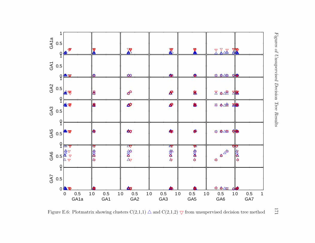
Fig
ures
ofU
nsu
perv
isedD
ecision
Tree
Resu
lts171
0 0.5 1GA7
0 0.5 1GA6
0 0.5 1GA5
0 0.5 1GA3
0 0.5 1GA2
0 0.5 1GA1
0 0.5 10
0.5
1
GA1a
GA
7
0
0.5
1
GA
6
0
0.5
1
GA
5
0
0.5
1
GA
3
0
0.5
1
GA
2
0
0.5
1G
A1
0
0.5
1
GA
1a
Figure E.6: Plotmatrix showing clusters C(2,1,1)4 and C(2,1,2)5 from unsupervised decision tree method
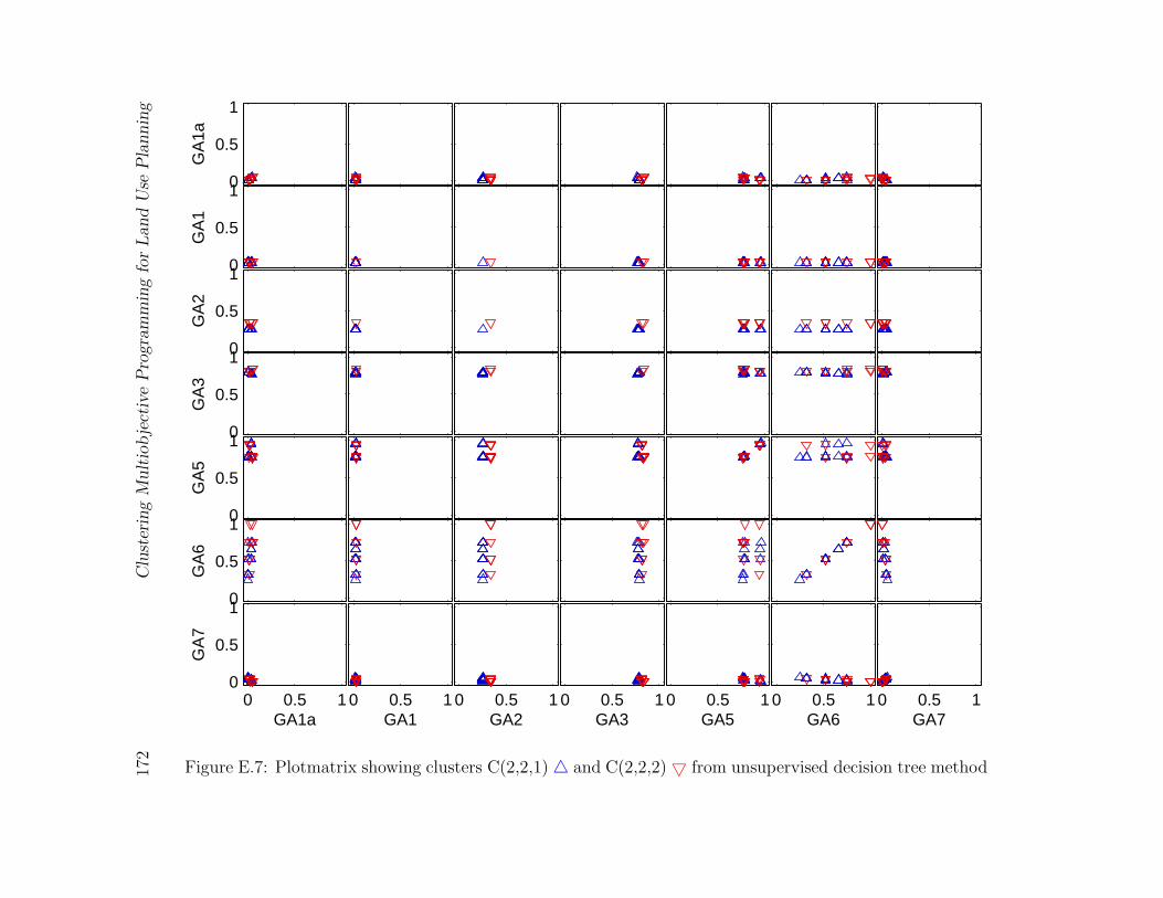
172
Clu
ster
ing
Mult
iobje
ctiv
eP
rogra
mm
ing
for
Land
Use
Pla
nnin
g
0 0.5 1GA7
0 0.5 1GA6
0 0.5 1GA5
0 0.5 1GA3
0 0.5 1GA2
0 0.5 1GA1
0 0.5 10
0.5
1
GA1a
GA
7
0
0.5
1
GA
6
0
0.5
1
GA
5
0
0.5
1
GA
3
0
0.5
1
GA
2
0
0.5
1G
A1
0
0.5
1
GA
1a
Figure E.7: Plotmatrix showing clusters C(2,2,1)4 and C(2,2,2)5 from unsupervised decision tree method
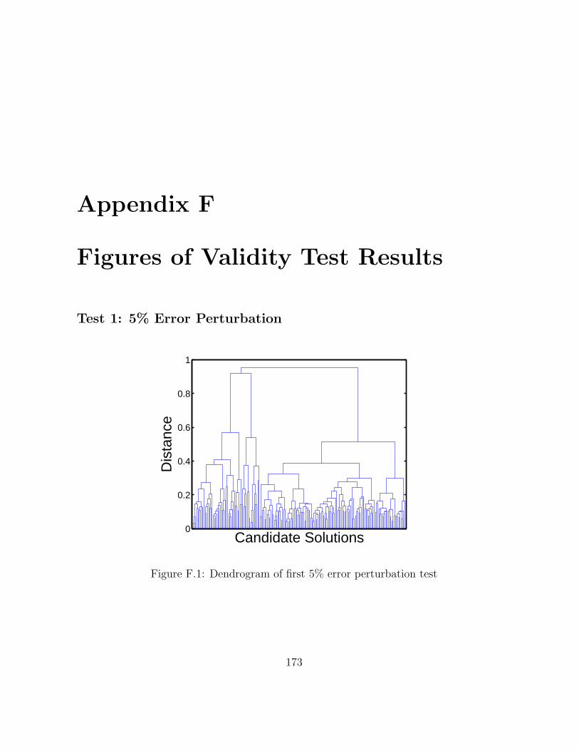
Appendix F
Figures of Validity Test Results
Test 1: 5% Error Perturbation
0
0.2
0.4
0.6
0.8
1
Candidate Solutions
Dis
tanc
e
Figure F.1: Dendrogram of first 5% error perturbation test
173
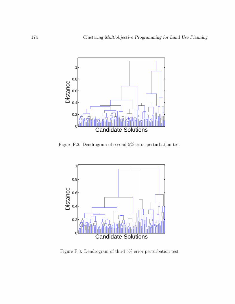
174 Clustering Multiobjective Programming for Land Use Planning
0
0.2
0.4
0.6
0.8
1
Candidate Solutions
Dis
tanc
e
Figure F.2: Dendrogram of second 5% error perturbation test
0
0.2
0.4
0.6
0.8
1
Candidate Solutions
Dis
tanc
e
Figure F.3: Dendrogram of third 5% error perturbation test
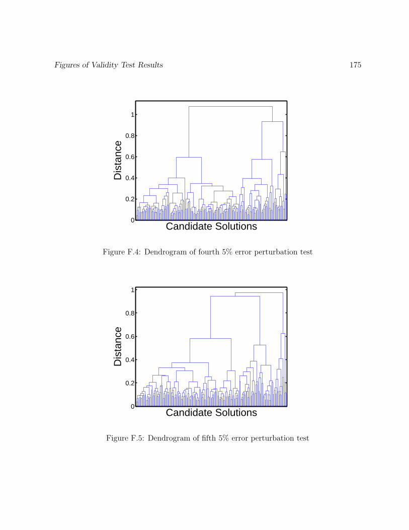
Figures of Validity Test Results 175
0
0.2
0.4
0.6
0.8
1
Candidate Solutions
Dis
tanc
e
Figure F.4: Dendrogram of fourth 5% error perturbation test
0
0.2
0.4
0.6
0.8
1
Candidate Solutions
Dis
tanc
e
Figure F.5: Dendrogram of fifth 5% error perturbation test
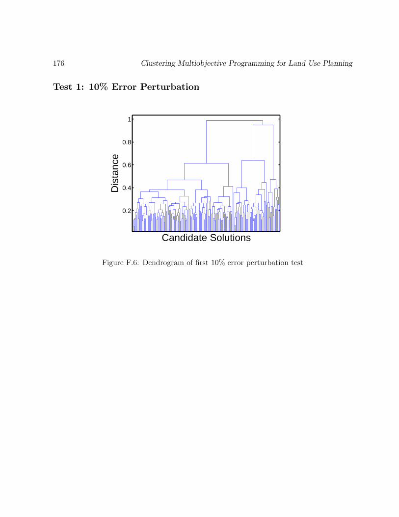
176 Clustering Multiobjective Programming for Land Use Planning
Test 1: 10% Error Perturbation
0.2
0.4
0.6
0.8
1
Candidate Solutions
Dis
tanc
e
Figure F.6: Dendrogram of first 10% error perturbation test
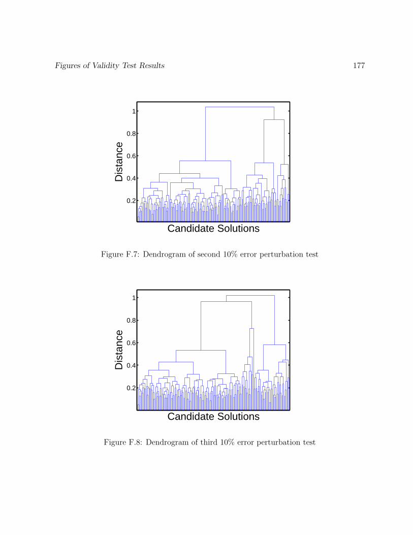
Figures of Validity Test Results 177
0.2
0.4
0.6
0.8
1
Candidate Solutions
Dis
tanc
e
Figure F.7: Dendrogram of second 10% error perturbation test
0.2
0.4
0.6
0.8
1
Candidate Solutions
Dis
tanc
e
Figure F.8: Dendrogram of third 10% error perturbation test
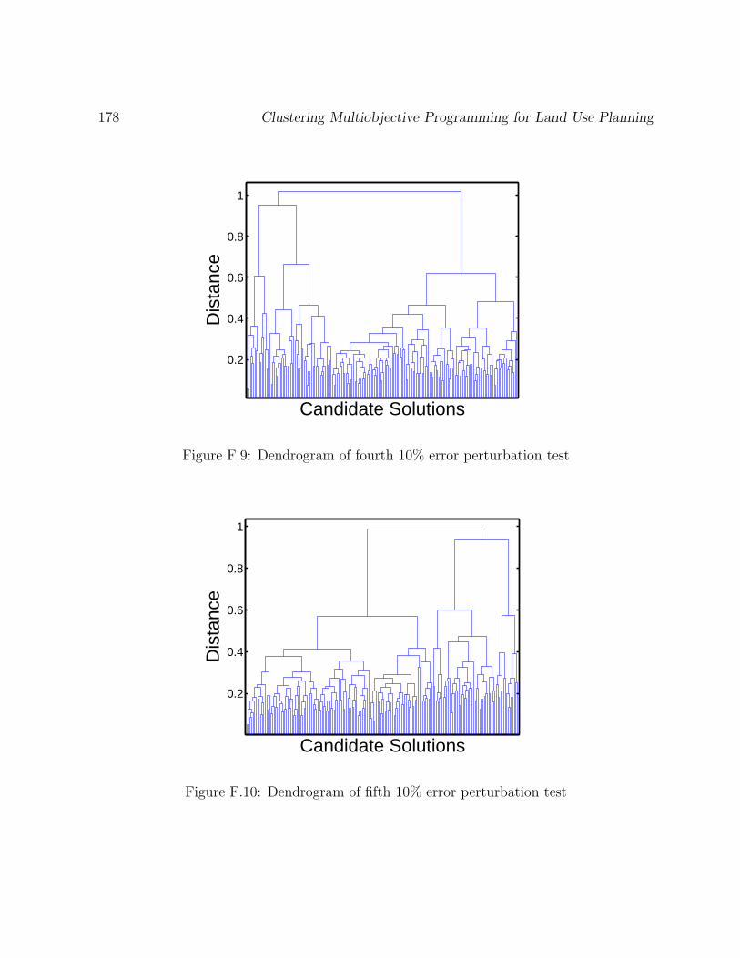
178 Clustering Multiobjective Programming for Land Use Planning
0.2
0.4
0.6
0.8
1
Candidate Solutions
Dis
tanc
e
Figure F.9: Dendrogram of fourth 10% error perturbation test
0.2
0.4
0.6
0.8
1
Candidate Solutions
Dis
tanc
e
Figure F.10: Dendrogram of fifth 10% error perturbation test
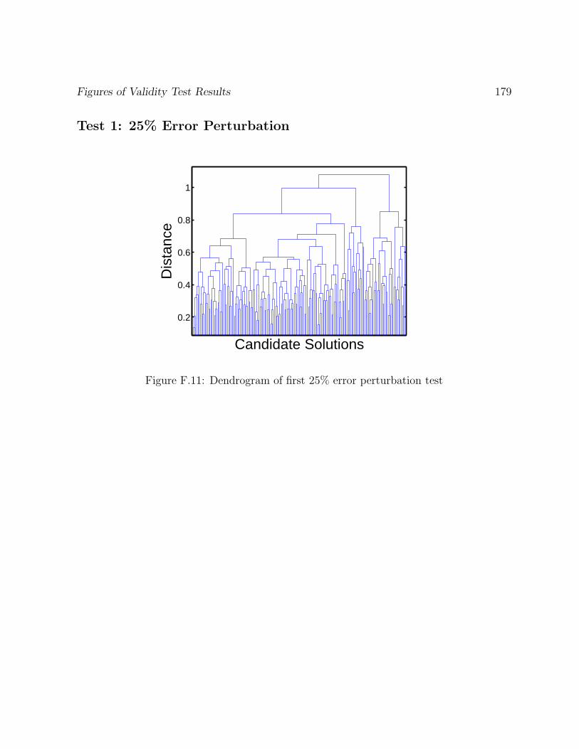
Figures of Validity Test Results 179
Test 1: 25% Error Perturbation
0.2
0.4
0.6
0.8
1
Candidate Solutions
Dis
tanc
e
Figure F.11: Dendrogram of first 25% error perturbation test
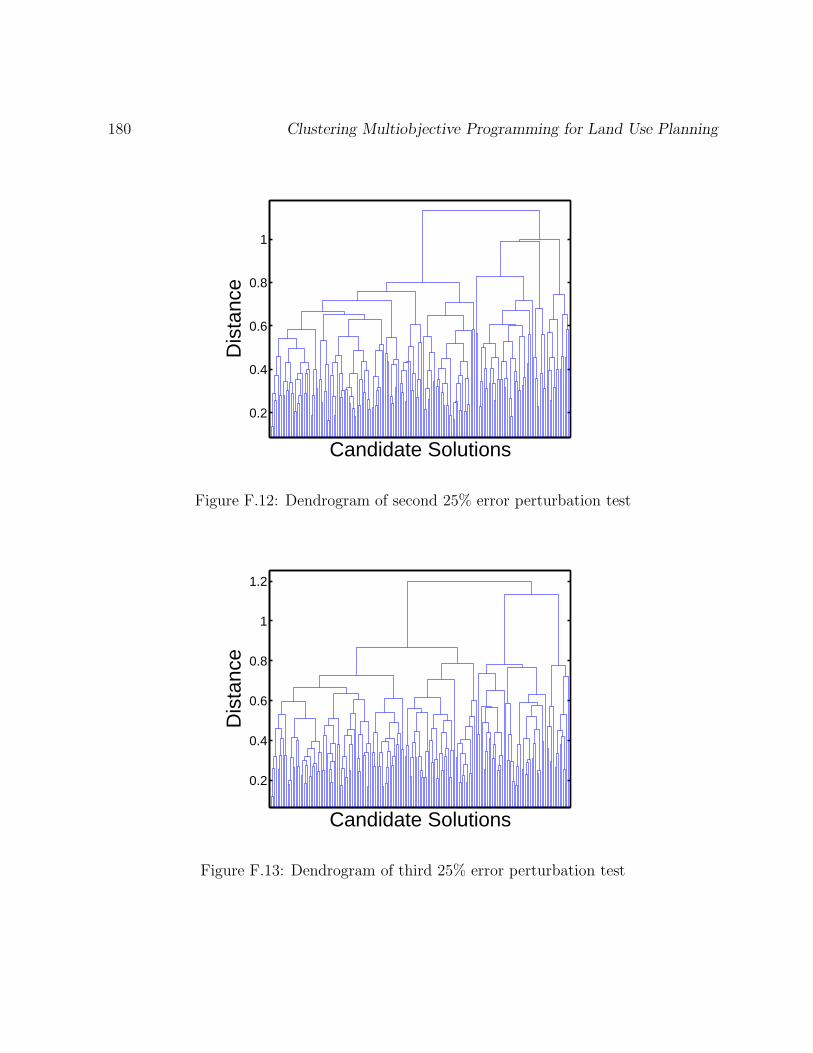
180 Clustering Multiobjective Programming for Land Use Planning
0.2
0.4
0.6
0.8
1
Candidate Solutions
Dis
tanc
e
Figure F.12: Dendrogram of second 25% error perturbation test
0.2
0.4
0.6
0.8
1
1.2
Candidate Solutions
Dis
tanc
e
Figure F.13: Dendrogram of third 25% error perturbation test
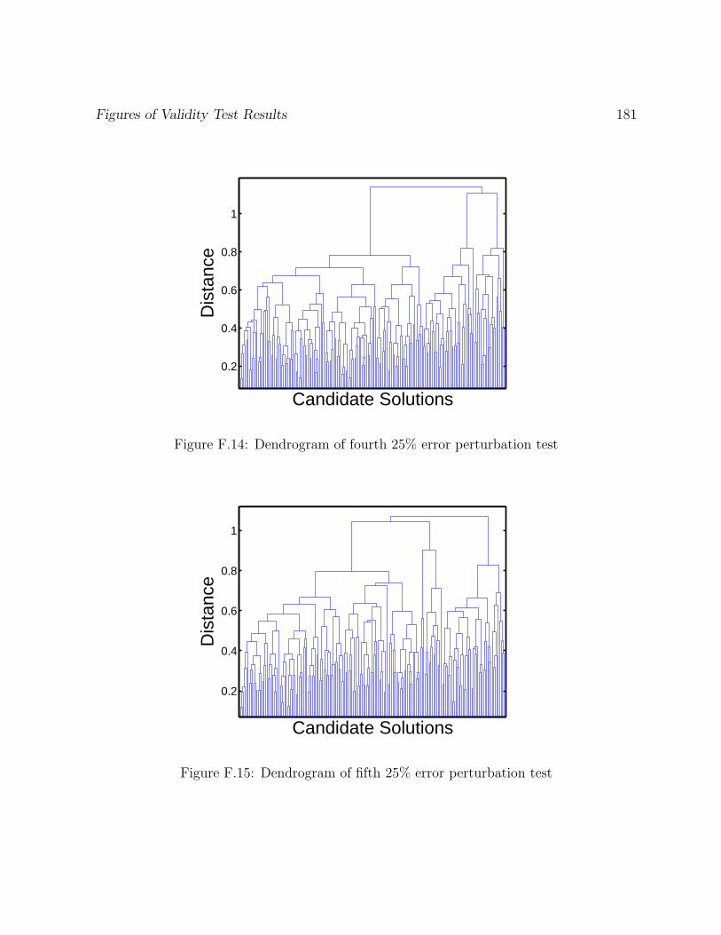
Figures of Validity Test Results 181
0.2
0.4
0.6
0.8
1
Candidate Solutions
Dis
tanc
e
Figure F.14: Dendrogram of fourth 25% error perturbation test
0.2
0.4
0.6
0.8
1
Candidate Solutions
Dis
tanc
e
Figure F.15: Dendrogram of fifth 25% error perturbation test

182 Clustering Multiobjective Programming for Land Use Planning
Test 2: 5% Data Deletion
0
0.1
0.2
0.3
0.4
0.5
0.6
0.7
0.8
0.9
1
Candidate Solutions
Dis
tanc
e
Figure F.16: Dendrogram of first 5% data deletion test
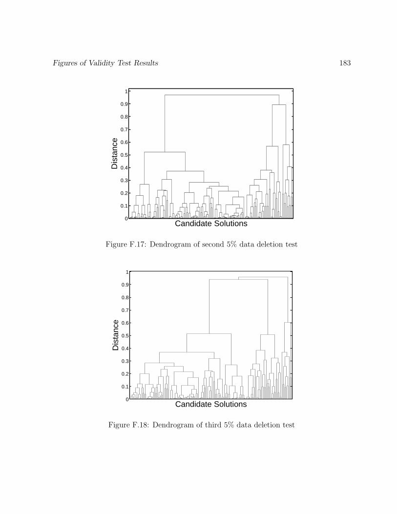
Figures of Validity Test Results 183
0
0.1
0.2
0.3
0.4
0.5
0.6
0.7
0.8
0.9
1
Candidate Solutions
Dis
tanc
e
Figure F.17: Dendrogram of second 5% data deletion test
0
0.1
0.2
0.3
0.4
0.5
0.6
0.7
0.8
0.9
1
Candidate Solutions
Dis
tanc
e
Figure F.18: Dendrogram of third 5% data deletion test
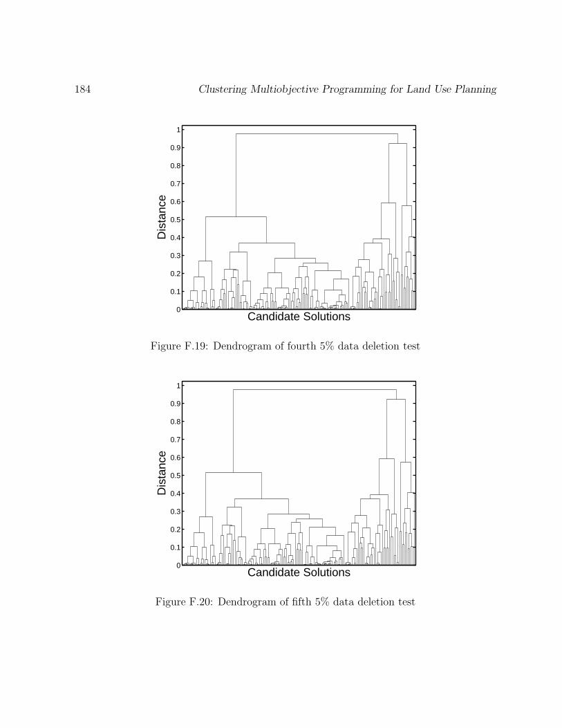
184 Clustering Multiobjective Programming for Land Use Planning
0
0.1
0.2
0.3
0.4
0.5
0.6
0.7
0.8
0.9
1
Candidate Solutions
Dis
tanc
e
Figure F.19: Dendrogram of fourth 5% data deletion test
0
0.1
0.2
0.3
0.4
0.5
0.6
0.7
0.8
0.9
1
Candidate Solutions
Dis
tanc
e
Figure F.20: Dendrogram of fifth 5% data deletion test
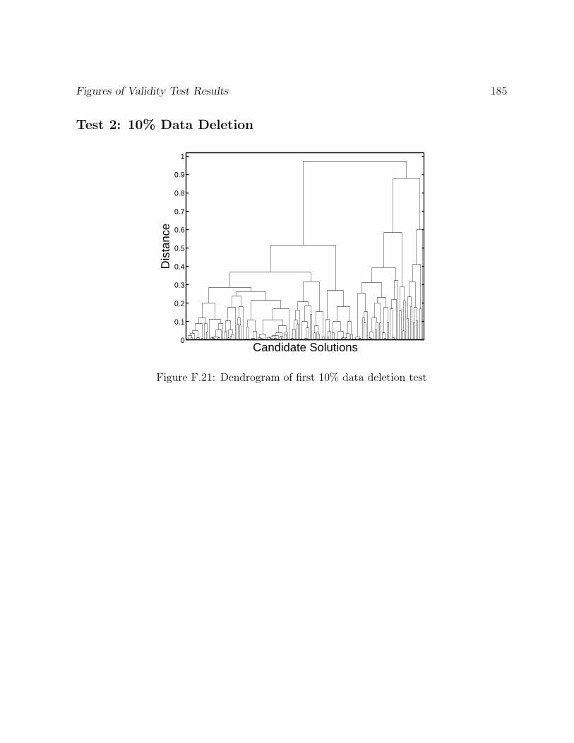
Figures of Validity Test Results 185
Test 2: 10% Data Deletion
0
0.1
0.2
0.3
0.4
0.5
0.6
0.7
0.8
0.9
1
Candidate Solutions
Dis
tanc
e
Figure F.21: Dendrogram of first 10% data deletion test
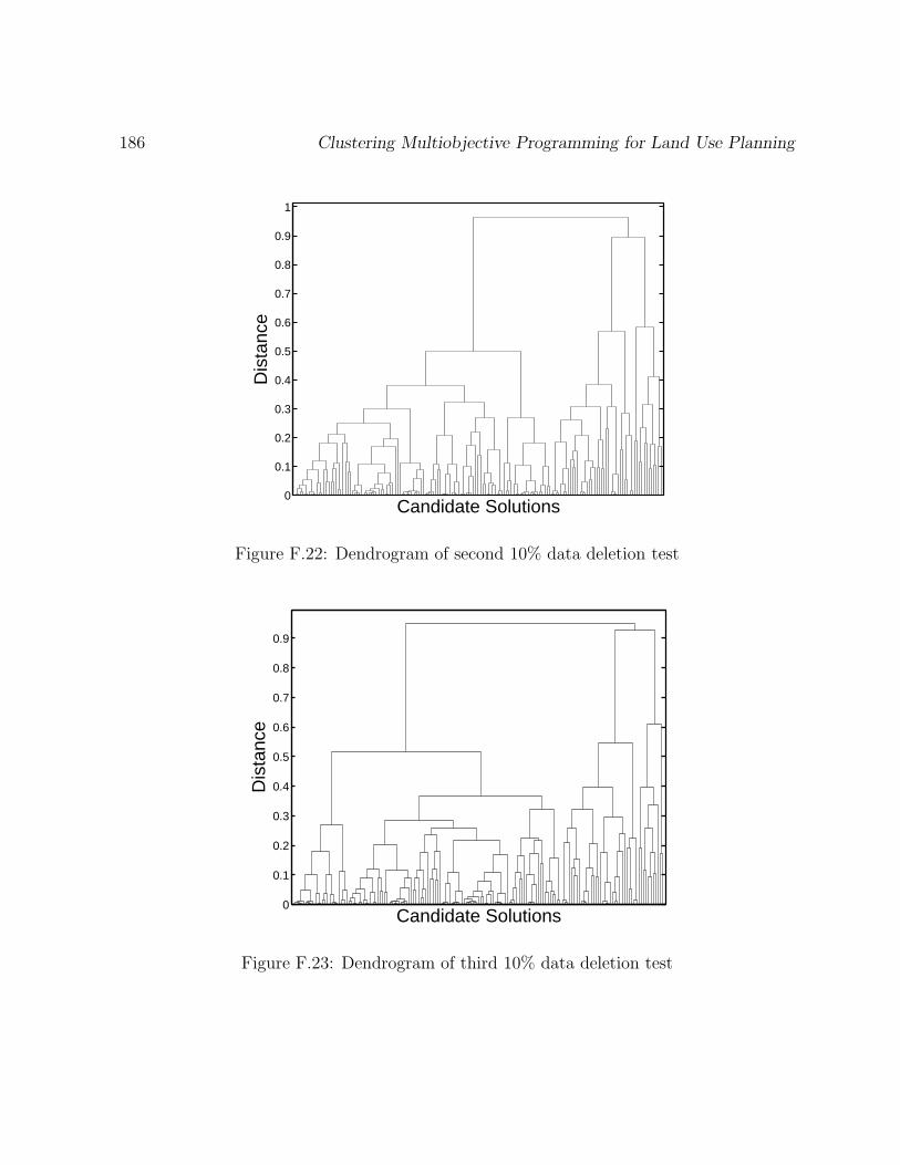
186 Clustering Multiobjective Programming for Land Use Planning
0
0.1
0.2
0.3
0.4
0.5
0.6
0.7
0.8
0.9
1
Candidate Solutions
Dis
tanc
e
Figure F.22: Dendrogram of second 10% data deletion test
0
0.1
0.2
0.3
0.4
0.5
0.6
0.7
0.8
0.9
Candidate Solutions
Dis
tanc
e
Figure F.23: Dendrogram of third 10% data deletion test
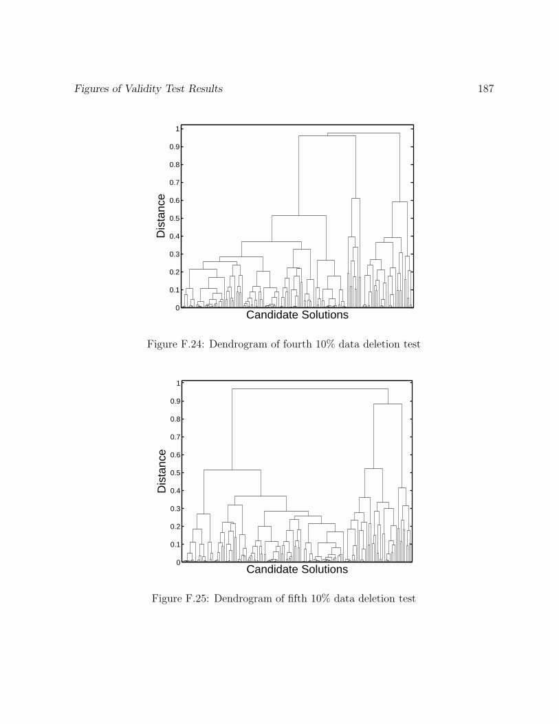
Figures of Validity Test Results 187
0
0.1
0.2
0.3
0.4
0.5
0.6
0.7
0.8
0.9
1
Candidate Solutions
Dis
tanc
e
Figure F.24: Dendrogram of fourth 10% data deletion test
0
0.1
0.2
0.3
0.4
0.5
0.6
0.7
0.8
0.9
1
Candidate Solutions
Dis
tanc
e
Figure F.25: Dendrogram of fifth 10% data deletion test
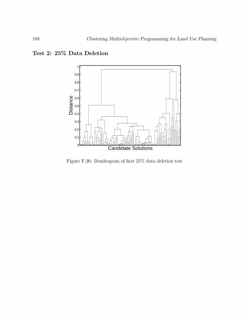
188 Clustering Multiobjective Programming for Land Use Planning
Test 2: 25% Data Deletion
0
0.1
0.2
0.3
0.4
0.5
0.6
0.7
0.8
0.9
1
Candidate Solutions
Dis
tanc
e
Figure F.26: Dendrogram of first 25% data deletion test

Figures of Validity Test Results 189
0
0.1
0.2
0.3
0.4
0.5
0.6
0.7
0.8
0.9
1
Candidate Solutions
Dis
tanc
e
Figure F.27: Dendrogram of second 25% data deletion test
0
0.1
0.2
0.3
0.4
0.5
0.6
0.7
0.8
0.9
1
Candidate Solutions
Dis
tanc
e
Figure F.28: Dendrogram of third 25% data deletion test
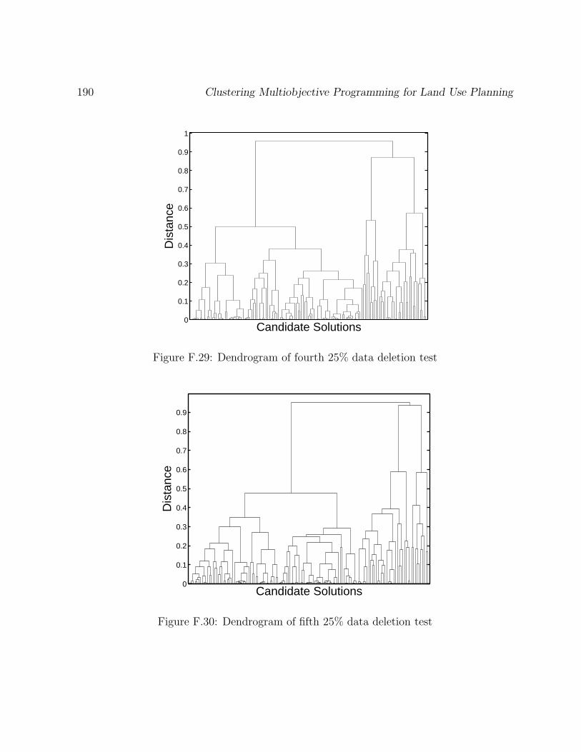
190 Clustering Multiobjective Programming for Land Use Planning
0
0.1
0.2
0.3
0.4
0.5
0.6
0.7
0.8
0.9
1
Candidate Solutions
Dis
tanc
e
Figure F.29: Dendrogram of fourth 25% data deletion test
0
0.1
0.2
0.3
0.4
0.5
0.6
0.7
0.8
0.9
Candidate Solutions
Dis
tanc
e
Figure F.30: Dendrogram of fifth 25% data deletion test

Figures of Validity Test Results 191
Test 3: Data Split
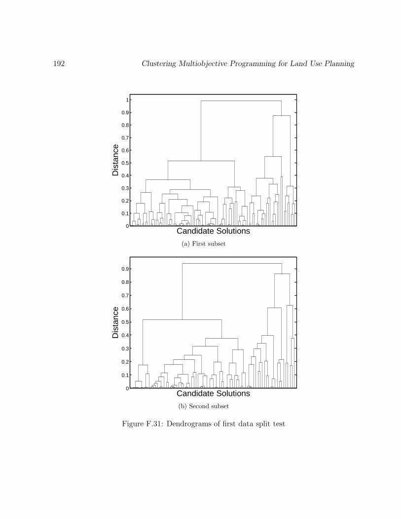
192 Clustering Multiobjective Programming for Land Use Planning
0
0.1
0.2
0.3
0.4
0.5
0.6
0.7
0.8
0.9
1
Candidate Solutions
Dis
tanc
e
(a) First subset
0
0.1
0.2
0.3
0.4
0.5
0.6
0.7
0.8
0.9
Candidate Solutions
Dis
tanc
e
(b) Second subset
Figure F.31: Dendrograms of first data split test
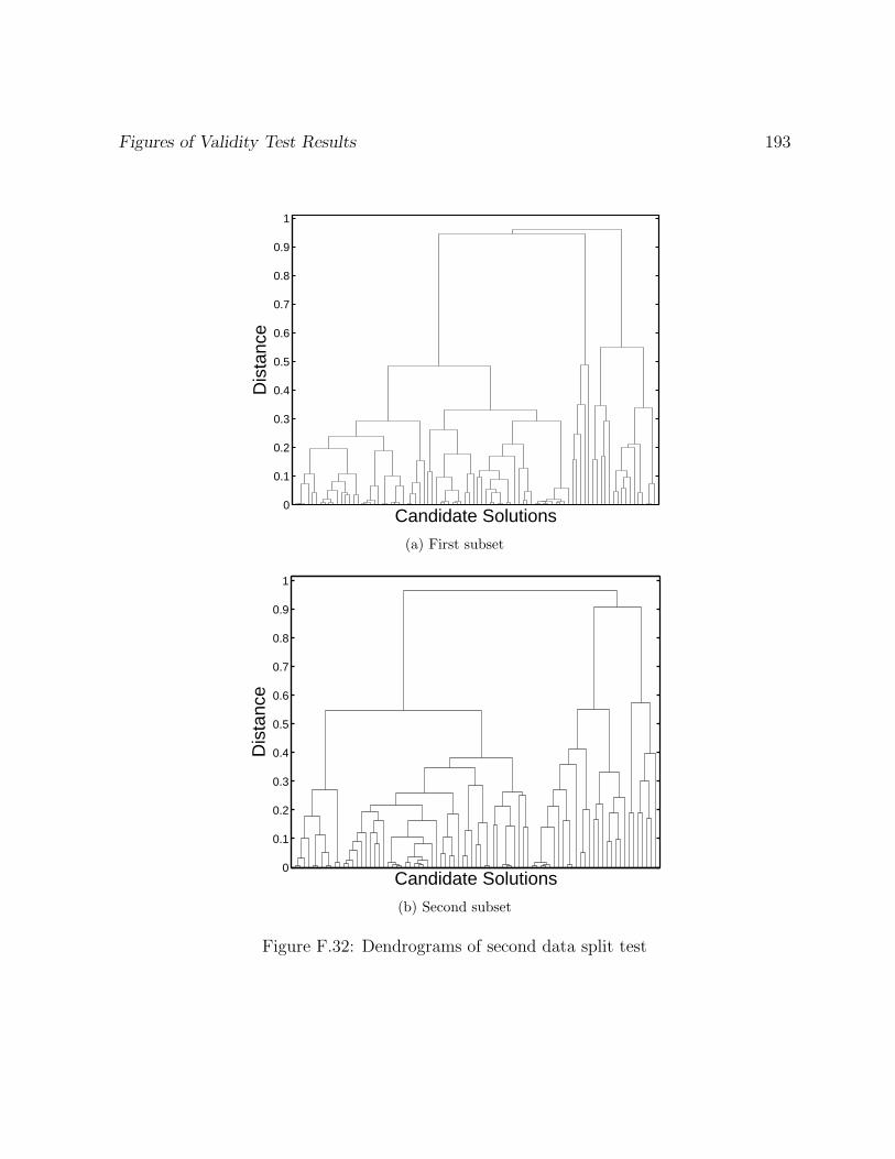
Figures of Validity Test Results 193
0
0.1
0.2
0.3
0.4
0.5
0.6
0.7
0.8
0.9
1
Candidate Solutions
Dis
tanc
e
(a) First subset
0
0.1
0.2
0.3
0.4
0.5
0.6
0.7
0.8
0.9
1
Candidate Solutions
Dis
tanc
e
(b) Second subset
Figure F.32: Dendrograms of second data split test
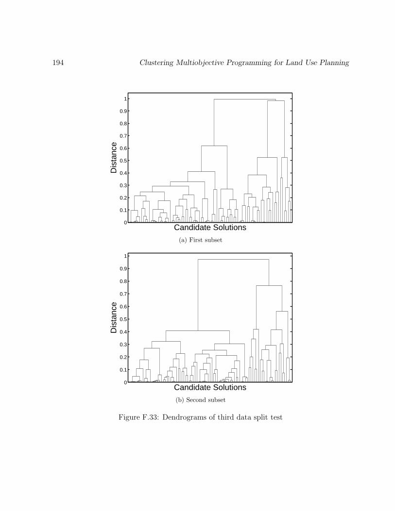
194 Clustering Multiobjective Programming for Land Use Planning
0
0.1
0.2
0.3
0.4
0.5
0.6
0.7
0.8
0.9
1
Candidate Solutions
Dis
tanc
e
(a) First subset
0
0.1
0.2
0.3
0.4
0.5
0.6
0.7
0.8
0.9
1
Candidate Solutions
Dis
tanc
e
(b) Second subset
Figure F.33: Dendrograms of third data split test
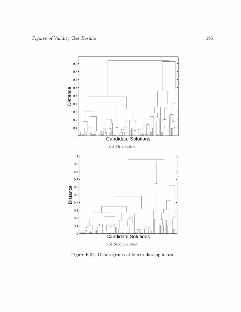
Figures of Validity Test Results 195
0
0.1
0.2
0.3
0.4
0.5
0.6
0.7
0.8
0.9
Candidate Solutions
Dis
tanc
e
(a) First subset
0
0.1
0.2
0.3
0.4
0.5
0.6
0.7
0.8
0.9
1
Candidate Solutions
Dis
tanc
e
(b) Second subset
Figure F.34: Dendrograms of fourth data split test
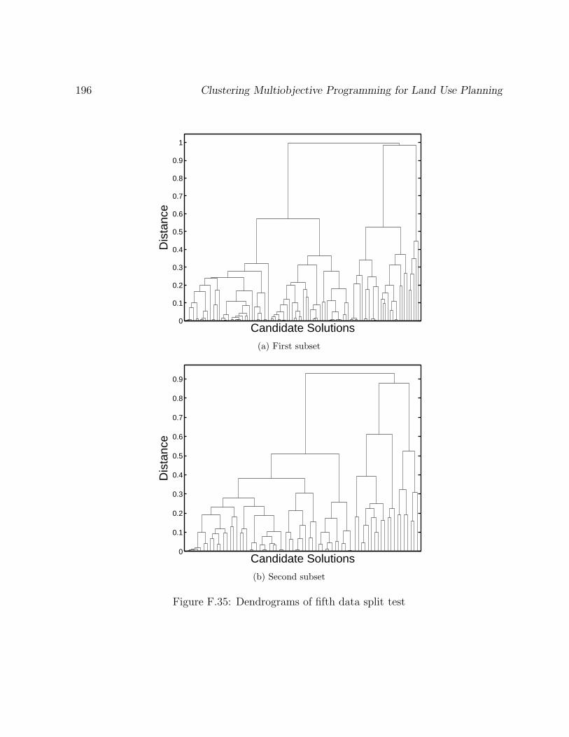
196 Clustering Multiobjective Programming for Land Use Planning
0
0.1
0.2
0.3
0.4
0.5
0.6
0.7
0.8
0.9
1
Candidate Solutions
Dis
tanc
e
(a) First subset
0
0.1
0.2
0.3
0.4
0.5
0.6
0.7
0.8
0.9
Candidate Solutions
Dis
tanc
e
(b) Second subset
Figure F.35: Dendrograms of fifth data split test
Related Documents