Hidden Markov Models - Northwestern Engineeringddowney/courses/474_Fall2017/hmms.pdf · Hidden Markov Models as Bayes Nets ... 1 according to prob e 1 (x 1) 3. Go to state ...

Hidden Markov Models

1

2

K

…

1

2

K

…

1

2

K

…

…

…

…

1

2

K

…

x1 x2 x3 xN

2

1

K

2

Example: The dishonest casino

A casino has two dice:

• Fair die

P(1) = P(2) = P(3) = P(4) = P(5) = P(6) = 1/6

• Loaded die

P(1) = P(2) = P(3) = P(4) = P(5) = 1/10

P(6) = 1/2

Casino player switches between fair and loaded die with probability 1/20 at each turn

Game:

1. You bet $1

2. You roll (always with a fair die)

3. Casino player rolls (maybe with fair die, maybe with loaded die)

4. Highest number wins $2

Question # 1 – Evaluation

GIVEN

A sequence of rolls by the casino player

1245526462146146136136661664661636616366163616515615115146123562344

QUESTION

How likely is this sequence, given our model of how the casino works?

This is the EVALUATION problem in HMMs

Prob = 1.3 x 10-35

Question # 2 – Decoding

GIVEN

A sequence of rolls by the casino player

1245526462146146136136661664661636616366163616515615115146123562344

QUESTION

What portion of the sequence was generated with the fair die, and what

portion with the loaded die?

This is the DECODING question in HMMs

FAIR LOADED FAIR

Question # 3 – Learning

GIVEN

A sequence of rolls by the casino player

1245526462146146136136661664661636616366163616515615115146123562344

QUESTION

How “loaded” is the loaded die? How “fair” is the fair die? How often

does the casino player change from fair to loaded, and back?

This is the LEARNING question in HMMs

Prob(6) = 64%

The dishonest casino model

FAIR LOADED

0.05

0.05

0.950.95

P(1|F) = 1/6

P(2|F) = 1/6

P(3|F) = 1/6

P(4|F) = 1/6

P(5|F) = 1/6

P(6|F) = 1/6

P(1|L) = 1/10

P(2|L) = 1/10

P(3|L) = 1/10

P(4|L) = 1/10

P(5|L) = 1/10

P(6|L) = 1/2

A Hidden Markov Model: we never observe the state, only

observe output dependent (probabilistically) on state

A parse of a sequence

Observation sequence x = x1……xN,

State sequence = 1, ……, N

1

2

K

…

1

2

K

…

1

2

K

…

…

…

…

1

2

K

…

x1 x2 x3 xN

2

1

K

2

An HMM is memoryless

At each time step t,

the only thing that affects future states

is the current state t

P(t+1 = k | “whatever happened so far”) =

P(t+1 = k | 1, 2, …, t, x1, x2, …, xt) =

P(t+1 = k | t)

K

1

…

2

An HMM is memoryless

At each time step t,

the only thing that affects xt

is the current state t

P(xt = b | “whatever happened so far”) =

P(xt = b | 1, 2, …, t, x1, x2, …, xt-1) =

P(xt = b | t)

K

1

…

2

Definition of a hidden Markov model

Definition: A hidden Markov model (HMM)

• Alphabet = { b1, b2, …, bM } = Val(xt)

• Set of states Q = { 1, ..., K } ….= Val(t)

• Transition probabilities between any two states

aij = transition prob from state i to state j

ai1 + … + aiK = 1, for all states i = 1…K

• Start probabilities a0i

a01 + … + a0K = 1

• Emission probabilities within each state

ek(b) = P( xt = b | t = k)

ek(b1) + … + ek(bM) = 1, for all states k = 1…K

K

1

…

2

Hidden Markov Models as Bayes Nets

i i+1 i+2 i+3

xi xi+1 xi+2 xi+3

6 5 2 4

States – unobserved

Observations

• Transition probabilities between any two states

ajk = transition prob from state j to state k

= P(i+1 = k | i = j)

• Emission probabilities within each state

ek(b) = P( xi = b | i = k)

How “special” of a case are HMM BNs?

• Template-based representation

All hidden nodes have same CPTs, as do all output nodes

• Limited connectivity

Junction tree has clique nodes of size <=

…2

• Special-purpose algorithms are simple and efficient

HMMs are good for…

• Speech Recognition

• Gene Sequence Matching

• Text Processing

Part of speech tagging

Information extraction

Handwriting recognition

Generating a sequence by the model

Given a HMM, we can generate a sequence of length n as follows:

1. Start at state 1 according to prob a01

2. Emit letter x1 according to prob e1(x1)

3. Go to state 2 according to prob a12

4. … until emitting xn

1

2

K

…

1

2

K

…

1

2

K

…

…

…

…

1

2

K

…

x1 x2 x3 xn

2

1

K

2

0

e2(x1)

a02

What did we call this earlier, for general Bayes Nets?

A parse of a sequence

Given a sequence x = x1……xN,

A parse of x is a sequence of states = 1, ……, N

1

2

K

…

1

2

K

…

1

2

K

…

…

…

…

1

2

K

…

x1 x2 x3 xN

2

1

K

2

Likelihood of a parse

Given a sequence x = x1……xN

and a parse = 1, ……, N,

To find how likely this scenario is:

(given our HMM)

P(x, ) = P(x1, …, xN, 1, ……, N) =

P(xN | N) P(N | N-1) ……P(x2 | 2) P(2 | 1) P(x1 | 1) P(1) =

a01 a12……aN-1N e1(x1)……eN(xN)

1

2

K

…

1

2

K

…

1

2

K

…

…

…

…

1

2

K

…

x1 x2 x3 xK

2

1

K

2

Example: the dishonest casino

Let the sequence of rolls be:

x = 1, 2, 1, 5, 6, 2, 1, 5, 2, 4

Then, what is the likelihood of

= Fair, Fair, Fair, Fair, Fair, Fair, Fair, Fair, Fair, Fair?

(say initial probs a0Fair = ½, a0Loaded = ½)

½ P(1 | Fair) P(Fair | Fair) P(2 | Fair) P(Fair | Fair) … P(4 | Fair) =

½ (1/6)10 (0.95)9 = .00000000521158647211 ~= 0.5 10-9

Example: the dishonest casino

So, the likelihood the die is fair in this run

is just 0.521 10-9

What is the likelihood of

= Loaded, Loaded, Loaded, Loaded, Loaded, Loaded, Loaded,

Loaded, Loaded, Loaded?

½ P(1 | Loaded) P(Loaded, Loaded) … P(4 | Loaded) =

½ (1/10)9 (1/2)1 (0.95)9 = .00000000015756235243 ~= 0.16 10-9

Therefore, it’s somewhat more likely that all the rolls are done with the

fair die, than that they are all done with the loaded die

Example: the dishonest casino

Let the sequence of rolls be:

x = 1, 6, 6, 5, 6, 2, 6, 6, 3, 6

Now, what is the likelihood = F, F, …, F?

½ (1/6)10 (0.95)9 ~= 0.5 10-9, same as before

What is the likelihood

= L, L, …, L?

½ (1/10)4 (1/2)6 (0.95)9 = .00000049238235134735 ~= 0.5 10-7

So, it is 100 times more likely the die is loaded

The three main questions for HMMs

1. Evaluation

GIVEN a HMM M, and a sequence x,

FIND Prob[ x | M ]

2. Decoding

GIVEN a HMM M, and a sequence x,

FIND the sequence of states that maximizes P[ x, | M ]

3. Learning

GIVEN a HMM M, with unspecified transition/emission probs.,

and a sequence x,

FIND parameters = (ei(.), aij) that maximize P[ x | ]

Problem 1: Evaluation

Compute the likelihood that a

sequence is generated by the model

Generating a sequence by the model

Given a HMM, we can generate a sequence of length n as follows:

1. Start at state 1 according to prob a01

2. Emit letter x1 according to prob e1(x1)

3. Go to state 2 according to prob a12

4. … until emitting xn

1

2

K

…

1

2

K

…

1

2

K

…

…

…

…

1

2

K

…

x1 x2 x3 xn

2

1

K

2

0

e2(x1)

a02

Evaluation

We will develop algorithms that allow us to compute:

P(x) Probability of x given the model

P(xi…xj) Probability of a substring of x given the model

P(i = k | x) “Posterior” probability that the ith state is k, given x

The Forward Algorithm

We want to calculate

P(x) = probability of x, given the HMM

Sum over all possible ways of generating x:

P(x) = P(x, ) = P(x | ) P()

To avoid summing over exponentially many paths , use variable

elimination. In HMMs, VE has same form at each i. Define:

fk(i) = P(x1…xi, i = k) (the forward probability)

“generate i first observations and end up in state k”

The Forward Algorithm – derivation

Define the forward probability:

fk(i) = P(x1…xi, i = k)

= 1…i-1 P(x1…xi-1, 1,…, i-1, i = k) ek(xi)

= j 1…i-2 P(x1…xi-1, 1,…, i-2, i-1 = j) ajk ek(xi)

= j P(x1…xi-1, i-1 = j) ajk ek(xi)

= ek(xi) j fj(i – 1) ajk

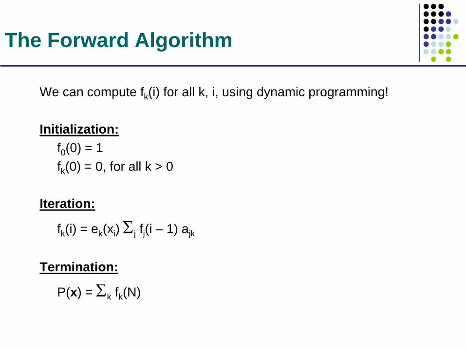
The Forward Algorithm

We can compute fk(i) for all k, i, using dynamic programming!

Initialization:

f0(0) = 1

fk(0) = 0, for all k > 0

Iteration:

fk(i) = ek(xi) j fj(i – 1) ajk

Termination:

P(x) = k fk(N)

Backward Algorithm

Forward algorithm can compute P(x). But we’d also like:

P(i = k | x),

the probability distribution on the ith position, given x

Again, we’ll use variable elimination. We start by computing:

P(i = k, x) = P(x1…xi, i = k, xi+1…xN)

= P(x1…xi, i = k) P(xi+1…xN | x1…xi, i = k)

= P(x1…xi, i = k) P(xi+1…xN | i = k)

Then, P(i = k | x) = P(i = k, x) / P(x)

Forward, fk(i) Backward, bk(i)

The Backward Algorithm – derivation

Define the backward probability:

bk(i) = P(xi+1…xN | i = k) “starting from ith state = k, generate rest of x”

= i+1…N P(xi+1,xi+2, …, xN, i+1, …, N | i = k)

= j i+2…N P(xi+1,xi+2, …, xN, i+1 = j, i+2, …, N | i = k)

= j ej(xi+1) akj i+2…N P(xi+2, …, xN, i+2, …, N | i+1 = j)

= j el(xi+1) akj bj(i+1)

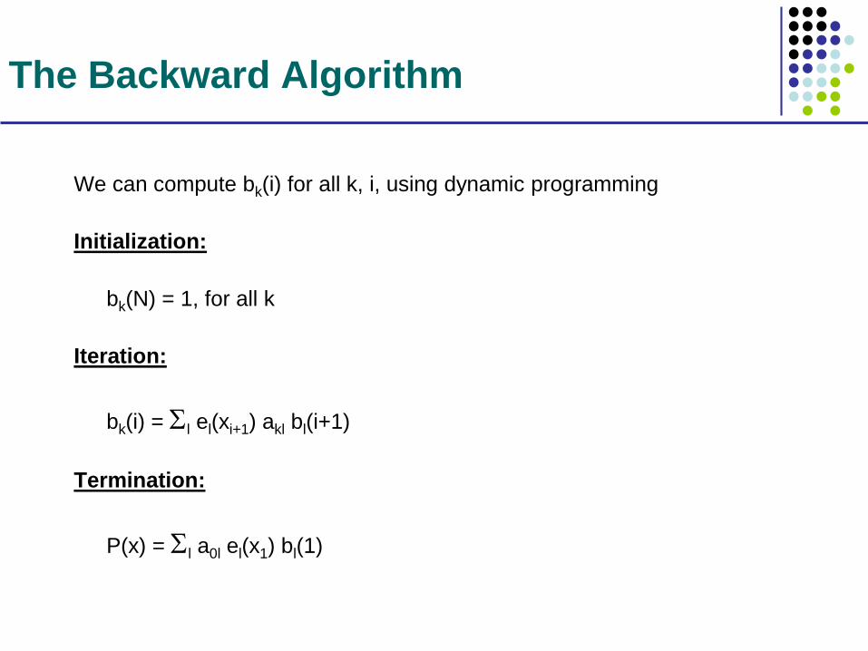
The Backward Algorithm

We can compute bk(i) for all k, i, using dynamic programming

Initialization:

bk(N) = 1, for all k

Iteration:

bk(i) = l el(xi+1) akl bl(i+1)

Termination:

P(x) = l a0l el(x1) bl(1)

Computational Complexity

What is the running time, and space required, for Forward and Backward?

Time: O(K2N)

Space: O(KN)

Useful implementation technique to avoid underflows:

rescaling at each few positions by multiplying

by a constant

Assuming we want to

save all forward,

backward messages.

Otherwise space can

be O(K)

Posterior Decoding

We can now calculate

fk(i) bk(i)

P(i = k | x) = –––––––

P(x)

Then, we can ask

What is the most likely state at position i of sequence x:

Define ^ by Posterior Decoding:

^i = argmaxk P(i = k | x)

P(i = k | x) =

P(i = k , x)/P(x) =

P(x1, …, xi, i = k, xi+1, … xn) / P(x) =

P(x1, …, xi, i = k) P(xi+1, … xn | i = k) / P(x) =

fk(i) bk(i) / P(x)

Posterior Decoding

x1 x2 x3 …………………………………………… xN

State 1

l P(i=j|x)

k

Problem 2: Decoding

Find the most likely parse

of a sequence

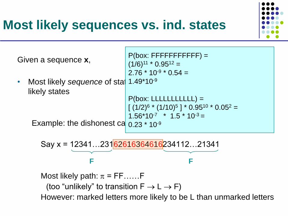
Most likely sequences vs. ind. states

Given a sequence x,

• Most likely sequence of states very different from sequence of most

likely states

Example: the dishonest casino

Say x = 12341…23162616364616234112…21341

Most likely path: = FF……F

(too “unlikely” to transition F L F)

However: marked letters more likely to be L than unmarked letters

P(box: FFFFFFFFFFF) =

(1/6)11 * 0.9512 =

2.76 * 10-9 * 0.54 =

1.49*10-9

P(box: LLLLLLLLLLL) =

[ (1/2)6 * (1/10)5 ] * 0.9510 * 0.052 =

1.56*10-7 * 1.5 * 10-3 =

0.23 * 10-9

F F

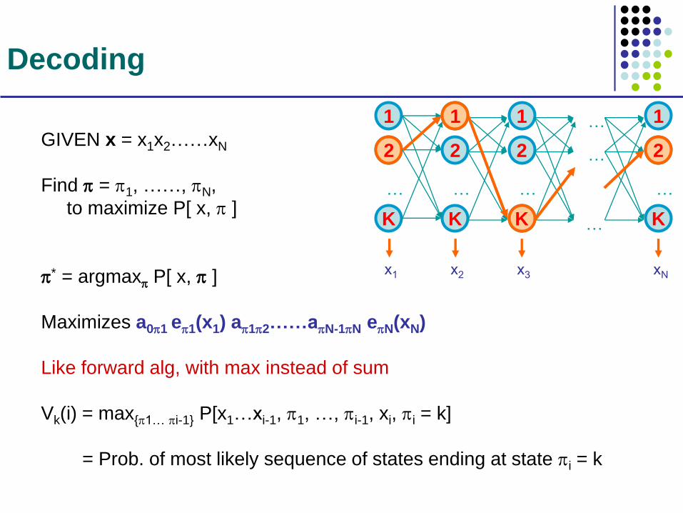
Decoding

GIVEN x = x1x2……xN

Find = 1, ……, N,

to maximize P[ x, ]

* = argmax P[ x, ]

Maximizes a01 e1(x1) a12……aN-1N eN(xN)

Like forward alg, with max instead of sum

Vk(i) = max{1… i-1} P[x1…xi-1, 1, …, i-1, xi, i = k]

= Prob. of most likely sequence of states ending at state i = k

1

2

K

…

1

2

K

…

1

2

K

…

…

…

…

1

2

K

…

x1 x2 x3 xN

2

1

K

2

Decoding – main idea

Induction: Given that for all states k, and for a fixed position i,

Vk(i) = max{1… i-1} P[x1…xi-1, 1, …, i-1, xi, i = k]

What is Vj(i+1)?

From definition,

Vl(i+1) = max{1… i}P[ x1…xi, 1, …, i, xi+1, i+1 = j ]

= max{1… i}P(xi+1, i+1 = j | x1…xi, 1,…, i) P[x1…xi, 1,…, i]

= max{1… i}P(xi+1, i+1 = j | i ) P[x1…xi-1, 1, …, i-1, xi, i]

= maxk [P(xi+1, i+1 = j | i=k) max{1… i-1}P[x1…xi-1,1,…,i-

1,xi,i=k]]

= maxk [ P(xi+1 | i+1 = j ) P(i+1 = j | i=k) Vk(i) ]= ej(xi+1) maxk akj Vk(i)

The Viterbi Algorithm

Input: x = x1……xN

Initialization:

V0(0) = 1 (0 is the imaginary first position)

Vk(0) = 0, for all k > 0

Iteration:

Vj(i) = ej(xi) maxk akj Vk(i – 1)

Ptrj(i) = argmaxk akj Vk(i – 1)

Termination:

P(x, *) = maxk Vk(N)

Traceback:

N* = argmaxk Vk(N)

i-1* = Ptri (i)

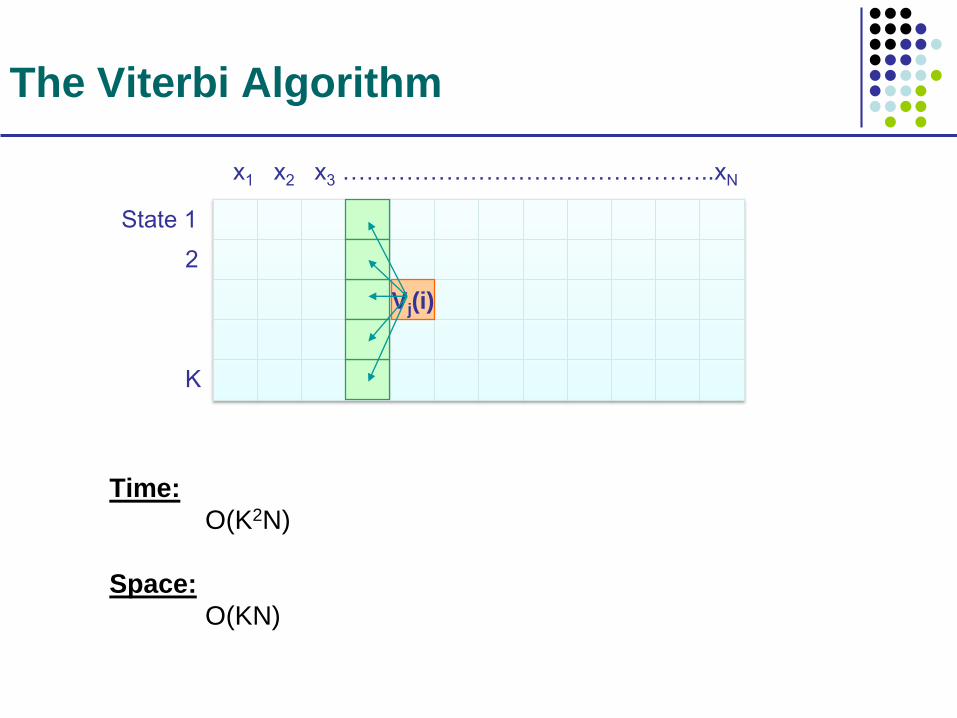
The Viterbi Algorithm

Time:

O(K2N)

Space:

O(KN)

x1 x2 x3 ………………………………………..xN

State 1

2

K

Vj(i)

Viterbi Algorithm – a practical detail

Underflows are a significant problem (like with forward, backward)

P[ x1,…., xi, 1, …, i ] = a01 a12……ai e1(x1)……ei(xi)

These numbers become extremely small – underflow

Solution: Take the logs of all values

Vl(i) = log ek(xi) + maxk [ Vk(i-1) + log akl ]

Example

Let x be a long sequence with a portion of ~ 1/6 6’s,

followed by a portion of ~ ½ 6’s…

x = 123456123456…12345 6626364656…1626364656

Then, it is not hard to show that optimal parse is:

FFF…………………...F LLL………………………...L

6 characters “123456” parsed as F, contribute .956(1/6)6 = 1.610-5

parsed as L, contribute .956(1/2)1(1/10)5 = 0.410-5

“162636” parsed as F, contribute .956(1/6)6 = 1.610-5

parsed as L, contribute .956(1/2)3(1/10)3 = 9.010-5

Viterbi, Forward, Backward

VITERBI

Initialization:

V0(0) = 1

Vk(0) = 0, for all k > 0

Iteration:

Vl(i) = el(xi) maxk Vk(i-1) akl

Termination:

P(x, *) = maxk Vk(N)

FORWARD

Initialization:

f0(0) = 1

fk(0) = 0, for all k > 0

Iteration:

fl(i) = el(xi) k fk(i-1) akl

Termination:

P(x) = k fk(N)

BACKWARD

Initialization:

bk(N) = 1, for all k

Iteration:

bl(i) = k el(xi+1) akl bk(i+1)

Termination:

P(x) = k a0k ek(x1) bk(1)

Problem 3: Learning

Find the parameters that maximize the likelihood of the

observed sequence

Estimating HMM parameters

• Easy if we know the sequence of hidden states

Count # times each transition occurs

Count #times each observation occurs in each state

• Given an HMM and observed sequence,

we can compute the distribution over paths,

and therefore the expected counts

• “Chicken and egg” problem

Solution: Use the EM algorithm

• Guess initial HMM parameters

• E step: Compute distribution over paths

• M step: Compute max likelihood parameters

• But how do we do this efficiently?

The forward-backward algorithm

• Also known as the Baum-Welch algorithm

• Compute probability of each state at each

position using forward and backward probabilities

→ (Expected) observation counts

• Compute probability of each pair of states at each

pair of consecutive positions i and i+1 using

forward(i) and backward(i+1)

→ (Expected) transition counts

Count(j→k) i fj(i) ajk bk(i+1)

Application: HMMs for

Information Extraction (IE)

• IE: Text machine-understandable data

Paris, the capital of France, …

(Paris, France) CapitalOf, p=0.85

• Applied to Web: better search engines, semantic Web, step toward human-level AI

IE Automatically?

Intractable to get human labels for every concept expressed

on the Web

Idea: extract from semantically tractable sentences

…Edison invented the light bulb…

(Edison, light bulb) Invented

x V y => (x, y) V

…Bloomberg, mayor of New York City…

(Bloomberg, New York City) Mayor

x, C of y => (x, y) C

Extraction patterns make errors:

“Erik Jonsson, CEO of Texas Instruments,

mayor of Dallas from 1964-1971, and…”

Extraction patterns make errors:

“Erik Jonsson, CEO of Texas Instruments,

mayor of Dallas from 1964-1971, and…”

48

But…

• Empirical fact:

Extractions you see over and over tend to be correct

The problem is the “long tail”

49

0

250

500

0 50000 100000

Frequency rank of extraction

Nu

mb

er

of

tim

es

ex

tra

cti

on

ap

pe

ars

in

pa

tte

rn

A mixture of correct and incorrect

e.g., (Dave Shaver, Pickerington)

(Ronald McDonald, McDonaldland)

Tend to be correct

e.g., (Bloomberg, New York City)

Challenge: the “long tail”

50

Mayor McCheese

51

Strategy

1) Model how common extractions occur in text

2) Rank sparse extractions by fit to model

Assessing Sparse Extractions

52

• Terms in the same class tend to appear in

similar contexts.

“cities including __” 42,000 1

“__ and other cities” 37,900 0

The Distributional Hypothesis

Hits with Hits withContext Chicago Twisp

“__ hotels” 2,000,000 1,670

“mayor of __” 657,000 82

53

• Precomputed – scalable

• Handle sparsity

HMM Language Models

54

…

cities such as Chicago , Boston ,

But Chicago isn’t the best

cities such as Chicago , Boston ,

Los Angeles and Chicago .

…

• Compute dot products between vectors of

common and sparse extractions [cf. Ravichandran et al. 2005]

1 2 1… …

Baseline: context vectors

55

ti ti+1 ti+2 ti+3

wi wi+1 wi+2 wi+3

cities such as Seattle

Hidden Markov Model (HMM)

States – unobserved

Words – observed

Hidden States ti {1, …, N} (N fairly small)

Train on unlabeled data

– P(ti | wi = w) is N-dim. distributional summary of w

– Compare extractions using KL divergence

56

Twisp: < >

P(t | Twisp):

Distributional Summary P(t | w)

Compact (efficient – 10-50x less data retrieved)

Dense (accurate – 23-46% error reduction)

. . . 0 0 0 1 . . .

0.14 0.01 … 0.06

t=1 2 N

HMM Compresses Context Vectors

57

Is Pickerington of the same type as Chicago?

Chicago , Illinois

Pickerington , Ohio

Chicago:

Pickerington:

=> Context vectors say no, dot product is 0!

291 0 …

0 1 …

Example

58

HMM Generalizes:

Chicago , Illinois

Pickerington , Ohio

Example

59

Task: Ranking sparse TextRunner extractions.

Metric: Area under precision-recall curve.

Language models reduce missing area by 39% over

nearest competitor.

Experimental Results

Headquartered Merged Average

Frequency 0.710 0.784 0.713

PL 0.651 0.851 … 0.785

LM 0.810 0.908 0.851

Example word distributions (1 of 2)

• P(word | state 3)

unk0 0.0244415

new 0.0235757

more 0.0123496

unk1 0.0119841

few 0.0114422

small 0.00858043

good 0.00806342

large 0.00736572

great 0.00728838

important 0.00710116

other 0.0067399

major 0.00628244

little 0.00545736

…

• P(word | state 24)

, 0.49014

. 0.433618

; 0.0079789

-- 0.00365591

- 0.00302614

! 0.00235752

: 0.001859

Example word distributions (2 of 2)

• P(word | state 1) unk1 0.116254

United+States 0.012609

world 0.009212

U.S 0.007950

University 0.007243

Internet 0.007152

time 0.005167

end 0.004928

unk0 0.004818

war 0.004260

country 0.003774

way 0.003528

city 0.003429

US 0.003269

Sun 0.002982

Earth 0.002628 …

• P(word | state 3) the 0.863846

a 0.0131049

an 0.00960474

its 0.008541

our 0.00650477

this 0.00366675

unk1 0.00313899

your 0.00265876

Correlation between LM and IE accuracy

Below: correlation coefficients

As LM error decreases, IE accuracy increases

Correlation between LM and IE accuracy

Correlation between LM and IE accuracy

What this suggests

• Better HMM language models => better information

extraction

• Better HMM language models => … => human-level

AI?

Consider: a good enough LM could do question answering,

pass the Turing Test, etc.

• There are lots of paths to human-level AI, but LMs

have:

Well-defined progress

Ridiculous amounts of training data

Also: active learning

• Today, people train language models by “taking

what comes”

Larger corpora => better language models

• But corpus size limited by # of humans typing

What if we asked for the most informative

sentences? (active learning)

What have we learned?

• In HMMs, general Bayes Net algorithms have

simple & efficient form1. Evaluation

GIVEN a HMM M, and a sequence x,

FIND Prob[ x | M ]

Forward Algorithm and Backward Algorithm (Variable Elimination)

2. Decoding

GIVEN a HMM M, and a sequence x,

FIND the sequence of states that maximizes P[ x, | M ]

Viterbi Algorithm (MAP query)

3. Learning

GIVEN A sequence x,

FIND HMM parameters = (ei(.), aij) that maximize P[ x | ]

Baum-Welch/Forward-Backward algorithm (EM)

What have we learned?

• Unsupervised Learning of HMMs can power

more scalable, accurate unsupervised IE

• Today, unsupervised learning of neural network

language models is much more popular

“Deep” networks – to be discussed in future weeks