International Journal of Computer Applications Technology and Research Volume 4– Issue 5, 336 - 339, 2015, ISSN:- 2319–8656 www.ijcat.com 336 Heuristic Algorithm for Efficient Data Retrieval Scheduling in the Multichannel Wireless Broadcast Environments A. Porselvi Dept. of CSE Panimalar Institute of Technology Chennai,India S.Brindha Devi Dept. of CSE Panimalar Institute of Technology Chennai,India Abstract: Wireless data broadcast is an efficient way of disseminating data to users in the mobile computing environments. From the server’s point of view, how to place the data items on channels is a crucial issue, with the objective of minimizing the average access time and tuning time. Similarly, how to schedule the data retrieval process for a given request at the client side such that all the requested items can be downloaded in a short time is also an important problem. In this paper, we investigate the multi-item data retrieval scheduling in the push-based multichannel broadcast environments. The most important issues in mobile computing are energy efficiency and query response efficiency. However, in data broadcast the objectives of reducing access latency and energy cost can be contradictive to each other. Consequently, we define a new problem named Minimum Cost Data Retrieval Problem (MCDR) and Large Number Data Retrieval (LNDR) Problem. We also develop a heuristic algorithm to download a large number of items efficiently. When there is no replicated item in a broadcast cycle, we show that an optimal retrieval schedule can be obtained in polynomial time. Keywords – Multichannel, Wireless data broadcast, MCDR, LNDR 1. INTRODUCTION BROADCAST is a means by which a single server can transmit data to an unlimited number of clients in a scalable way [3], [4]. Unlike unicast transmission, broadcast is scalable because a single transmission of an item satisfies all outstanding requests for it Generally, there are two types of broadcast systems: push-based and pull-based. In a push-based system, the server will broadcast a set of data items to the clients periodically according to a fixed schedule; while in a pull-based system, the clients will first send requests to the server and the server will provide timely broadcast according to the requests received. Response time is the time interval between the moment a client tunes in a broadcast system with a request of one or more data items to the moment all requested data are downloaded. It is obvious that shorter response time is more desirable. On the other hand, in wireless communication environments, most clients are mobile devices operating on batteries. The smaller the amount of energy consumed during retrieving data is, the longer the battery life of a mobile device will be. Therefore, saving energy is another important issue for designing wireless data broadcast system. The fast development of wireless communication technologies such as OFDM (Orthogonal frequency division multiplexing) makes efficiently broadcasting data through multiple channels possible [25]. How to allocate the data onto multiple channels to minimize the expected response time has become a hot research topic and lots of scheduling algorithms are proposed [11], [19], [21]. When a query requests only one data item, to schedule the retrieving process is straightforward. However, it is common that a query requests multiple data items at a time [9], [15], [18] (e.g., a user may submit a query of the top 10 stocks). In such cases, different retrieving schedules may result in different response time. Moreover, in a multi-channel broadcast system, retrieving data will probably need switchings among the channels, which not only consumes additional energy, but also causes possible conflicts [17], [22], [26]. The LNDR problem takes the “deadline” into consideration and therefore also describes the time-critical scenario. For push- based broadcast, we derive a polynomial time (1 − 1 −∈)- approximation scheme for LNDR, and we also propose a heuristic algorithm for it based on maximum independent set. For the case that all channels are synchronized, we propose a polynomial time optimal algorithm for LNDR. When channels are unsynchronized, we prove LNDR is NP- hard. When all the requested data items have to be downloaded, we formulate another problem, namely minimum cost data retrieval (MCDR), with the objective of minimizing the response time and energy consumption .We

Welcome message from author
This document is posted to help you gain knowledge. Please leave a comment to let me know what you think about it! Share it to your friends and learn new things together.
Transcript

International Journal of Computer Applications Technology and Research
Volume 4– Issue 5, 336 - 339, 2015, ISSN:- 2319–8656
www.ijcat.com 336
Heuristic Algorithm for Efficient Data Retrieval Scheduling in the Multichannel Wireless Broadcast
Environments
A. Porselvi
Dept. of CSE
Panimalar Institute of Technology
Chennai,India
S.Brindha Devi
Dept. of CSE
Panimalar Institute of Technology
Chennai,India
Abstract: Wireless data broadcast is an efficient way of disseminating data to users in the mobile computing environments.
From the server’s point of view, how to place the data items on channels is a crucial issue, with the objective of minimizing the
average access time and tuning time. Similarly, how to schedule the data retrieval process for a given request at the client side
such that all the requested items can be downloaded in a short time is also an important problem. In this paper, we investigate the
multi-item data retrieval scheduling in the push-based multichannel broadcast environments. The most important issues in mobile
computing are energy efficiency and query response efficiency. However, in data broadcast the objectives of reducing access
latency and energy cost can be contradictive to each other. Consequently, we define a new problem named Minimum Cost Data
Retrieval Problem (MCDR) and Large Number Data Retrieval (LNDR) Problem. We also develop a heuristic algorithm to
download a large number of items efficiently. When there is no replicated item in a broadcast cycle, we show that an optimal
retrieval schedule can be obtained in polynomial time.
Keywords – Multichannel, Wireless data broadcast, MCDR, LNDR
1. INTRODUCTION
BROADCAST is a means by which a single server can
transmit data to an unlimited number of clients in a scalable
way [3], [4]. Unlike unicast transmission, broadcast is
scalable because a single transmission of an item satisfies all
outstanding requests for it Generally, there are two types of
broadcast systems: push-based and pull-based.
In a push-based system, the server will broadcast
a set of data items to the clients periodically according to a
fixed schedule; while in a pull-based system, the clients will
first send requests to the server and the server will provide
timely broadcast according to the requests received.
Response time is the time interval between the moment a
client tunes in a broadcast system with a request of one or
more data items to the moment all requested data are
downloaded. It is obvious that shorter response time is more
desirable. On the other hand, in wireless communication
environments, most clients are mobile devices operating on
batteries. The smaller the amount of energy consumed
during retrieving data is, the longer the battery life of a
mobile device will be. Therefore, saving energy is another
important issue for designing wireless data broadcast
system. The fast development of wireless communication
technologies such as OFDM (Orthogonal frequency division
multiplexing) makes efficiently broadcasting data through
multiple channels possible [25]. How to allocate the data
onto multiple channels to minimize the expected response
time has become a hot research topic and lots of scheduling
algorithms are proposed [11], [19], [21]. When a query
requests only one data item, to schedule the retrieving
process is straightforward. However, it is common that a
query requests multiple data items at a time [9], [15], [18]
(e.g., a user may submit a query of the top 10 stocks). In such
cases, different retrieving schedules may result in different
response time. Moreover, in a multi-channel broadcast
system, retrieving data will probably need switchings among
the channels, which not only consumes additional energy,
but also causes possible conflicts [17], [22], [26]. The LNDR
problem takes the “deadline” into consideration and
therefore also describes the time-critical scenario. For push-
based broadcast, we derive a polynomial time (1 −1
𝑒−∈)-
approximation scheme for LNDR, and we also propose a
heuristic algorithm for it based on maximum independent
set. For the case that all channels are synchronized, we
propose a polynomial time optimal algorithm for LNDR.
When channels are unsynchronized, we prove LNDR is NP-
hard. When all the requested data items have to be
downloaded, we formulate another problem, namely
minimum cost data retrieval (MCDR), with the objective of
minimizing the response time and energy consumption .We
International Journal of Computer Applications Technology and Research
Volume 4– Issue 5, 336 - 339, 2015, ISSN:- 2319–8656
www.ijcat.com 337
investigate the approximability of MCDR in push-based
broadcast. Due to the strong in-approximability, we develop
a heuristic algorithm for MCDR.
2. RELATED WORKS
Scheduling is an important issue in the area of
wireless data broadcast. Acharya et al. first proposed the
scheduling problem for data broadcast [1], and Prabhakara
et al. suggested the multi-channel model for data broadcast
to improve the data delivery performance [14]. Since then,
many works have been done for scheduling data on multiple
channels to reduce the expected access time [20,22,2].
Besides, some researches began to study how to allocate
dependent data on broadcast channels (see, e.g.,
[10,19,21,5,6]). With respect to index, many methods have
been proposed to improve the search efficiency in data
broadcast systems (see, e.g., [8,16,18,19,21]).
Jung et al. proposed a tree-structured index
algorithm that allocates indices and data on different
channels [11]. Lo and Chen designed a parameterized
schema for allocating indices and data optimally on multiple
channels such that the average expected access latency is
minimized [12]. In terms of data retrieval scheduling,
Hurson et al. proposed two heuristic algorithms for
downloading multiple data items from multiple channels [7].
As both push-based and pull-based approaches have their
own strengths and drawbacks [15,16], hybrid scheduling is
regarded as a prospective approach to better scheduling.
N. Saxena et al. [17] proposed a probabilistic
hybrid scheduling, which probabilistically selects push
operation or pull operation based on the present system
statistics. Their results show that hybrid scheduling
generally outperforms other purely push-based or pull-based
algorithms in terms of access time. However, the above are
all non-real-time scheduling. Huang and Chen proposed a
scheme based on a generic algorithm to handle a similar
problem [5].
3. PROPOSED WORK In graph theory, an independent set or stable set
for a graph G is a subset of vertices that are pairwise non-
adjacent. A maximum independent set is an independent set
with the maximum cardinality. As we mentioned in Section
2, a valid retrieval schedule for an LNDR instance is a set of
triples without conflicts. Thus, finding a valid schedule with
the largest number of requested data items is equivalent to
finding a maximum independent set, considering conflicts as
edges and triples as vertices. Although finding a maximum
independent set is NP-hard, we still can devise heuristics that
provide solutions not necessarily provable, but usually
efficient for practice. We next present a sequential greedy
heuristic that guarantees a maximal valid retrieval schedule
(i.e., a valid set of triples that is not a subset of others).
Heuristic Algorithm: 1. Input: an LNDR instance which is represented by
a set of triples.
2. Construct a graph G of triples and add edges
between conflicted triples;
3. Let P<-Ø (P denotes the set of triples selected);
4. While G is not empty do
select a triple in G with the minimum degree;
put it in P and delete its neighbors;
5.end while
6.output P;
Generally, when a subset of elements need to be selected, a
greedy based algorithm will construct a solution by adding
elements sequentially. Decisions on which element is to be
added is based on certain rule. In SGH each time we add a
triple with the minimum degree. It can be shown that
choosing a vertex and removing its neighbors repeatedly will
achieve a maximal independent set. Thus, the solution
resulted by SGH is maximal. Moreover, based on our
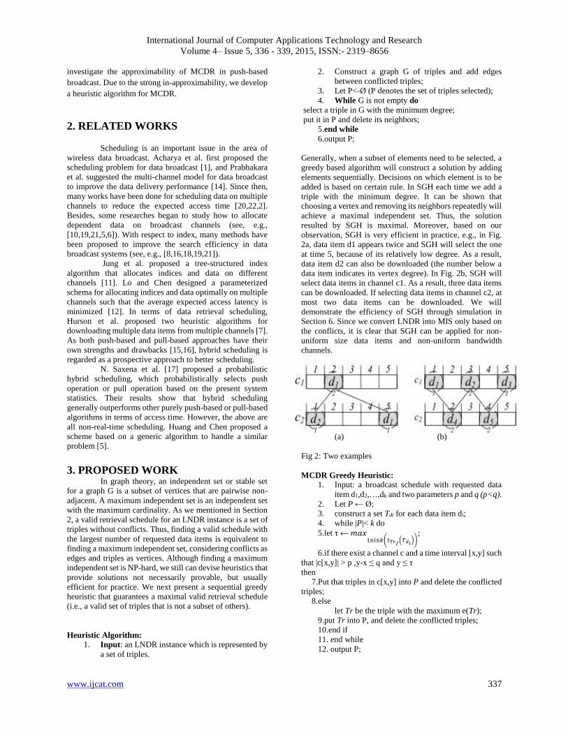
observation, SGH is very efficient in practice, e.g., in Fig.
2a, data item d1 appears twice and SGH will select the one
at time 5, because of its relatively low degree. As a result,
data item d2 can also be downloaded (the number below a
data item indicates its vertex degree). In Fig. 2b, SGH will
select data items in channel c1. As a result, three data items
can be downloaded. If selecting data items in channel c2, at
most two data items can be downloaded. We will
demonstrate the efficiency of SGH through simulation in
Section 6. Since we convert LNDR into MIS only based on
the conflicts, it is clear that SGH can be applied for non-
uniform size data items and non-uniform bandwidth
channels.
(a) (b)
Fig 2: Two examples
MCDR Greedy Heuristic: 1. Input: a broadcast schedule with requested data
item d1,d2,…,dk and two parameters p and q (p<q).
2. Let P ← Ø;
3. construct a set Tdi for each data item di;
4. while |P|< k do
5.let τ ← 𝑚𝑎𝑥1≤𝑖≤𝑘(𝑡𝑇𝑟𝑓(𝑇𝑑𝑖))
;
6.if there exist a channel c and a time interval [x,y] such
that |c[x,y]| > p ,y-x ≤ q and y ≤ τ
then
7.Put that triples in c[x,y] into P and delete the conflicted
triples;
8.else
let Tr be the triple with the maximum e(Tr);
9.put Tr into P, and delete the conflicted triples;
10.end if
11. end while
12. output P;

International Journal of Computer Applications Technology and Research
Volume 4– Issue 5, 336 - 339, 2015, ISSN:- 2319–8656
www.ijcat.com 338
1) Let [x,y] be a time interval and c be a channel, define
c[x,y] to be the set of data items in the time interval [x, y] of
channel c.
2) For each triple Tr= (dTr; cTr; tTr), define e(Tr) to be the
earliest time that data item dTr is downloadable if we do not
download Tr at time tTr.
3) For each requested data item d, define T d to be the set of
triples of d.
4) Let T be a set of triples, define Trf(T) and Tre(T),
respectively, to be the first and last triples in T according to
the broadcasting time.
In MGH (Algorithm 5), P holds the triples selected and t is
the earliest possible time that all the requested data items can
be downloaded. Each time MGH searches for a channel
broadcasting a significant number of data items during a
short time interval before t. If there exists such a channel, it
downloads those data items; otherwise, it selects a triple Tr
greedily with the maximum e(Tr). The two parameters p and
q would be chosen according to α, λActive, λDoze and λSwitch.
When α=0 and λDoze=0, we can ignore the response time and
set q to be greater than the cycle length, which converts the
MCDR problem into a set cover problem, and thus brings an
O(log k)-factor approximation solution. When α=1, we can
decrease q and increase p to minimize the response time,
regardless of the energy consumption.
4. CONCLUSION
In this paper, the data retrieval scheduling for
multi-item requests over multiple channels is studied. Two
optimization problems, LNDR and MCDR, are defined and
some approximation and heuristic algorithms are proposed.
The algorithms are analyzed both theoretically and
practically. Their efficiencies are also demonstrated through
simulation. For LNDR in push-based broadcast, MM can
download the maximum number of data items when the
channels are synchronized. When the channels are
unsynchronized, SGH always achieves a better solution with
respect to GL, NO, MM and RS, and it scales well. AS is
slightly better than SGH but it cannot be applied to download
a large number of data items. For LNDR in pull-based
broadcast, GL is better than NO, and other algorithms cannot
be applied. For MCDR, MGH always outperforms MH, GL,
NO and RS.
RS is also an efficient scheduling when a large
percentage of data items have to be downloaded. To the best
of our knowledge, we do not find any algorithms in the
literature which are designed for pull-based data scheduling
at the server side over multiple unsynchronized channels. As
a direction for further research, one can study the data
scheduling problem for unsynchronized channels from the
server’s point of view.
6. REFERENCES
[1] J.E. Hopcroft and R.M. Karp, “An n5=2 Algorithm for
Maximum Matchings in Bipartite Graphs,” SIAM J.
Computing, vol. 2, no. 4, pp. 225-231, 1973.
[2] H.D. Dykeman, M. Ammar, and J.W. Wong,
“Scheduling Algorithms for Videotex Systems under
Broadcast Delivery,” Proc. IEEE Int’l Conf. Comm., pp.
1847-1851, 1986.
[3] S. Acharya, R. Alonso, M. Franklin, and S. Zdonik,
“Broadcast
Disks: Data Management for Asymmetric Communication
Environments,” Proc. ACM SIGMOD Int’l Conf.
Management of Data, pp. 199-210, 1995.
[4] N. Vaidya and S. Hameed, “Log Time Algorithms for
Scheduling Single and Multiple Channel Data Broadcast,”
Proc. Ann. Int’l Conf. Mobile Computing and Networking,
pp. 90-99, 1997.
[5] U. Feige, “A Threshold of lnn for Approximating Set
Cover,” J. ACM, vol. 45, no. 4, pp. 314-318, 1998.
[6] T. Imielinski, S. Viswanathan, and B.R. Badrinath, “Data
on Air: Organization and Access,” IEEE Trans. Knowledge
and Data Eng., vol. 9, no. 3, pp. 353-372, May/June 1997.
[7] D. Aksoy and M. Franklin, “Scheduling for Large-Scale
On-Demand Data Broadcasting,” Proc. IEEE Int’l Conf.
Computer Comm., pp. 651-659, 1998.
[8] D. Aksoy and M. Franklin, “R _W: A Scheduling
Approach for Large-Scale On-Demand Data Broadcasting,”
IEEE/ACM Trans. Networking, vol. 7, no. 6, pp. 846-860,
Dec. 1999.
[9] C. Kenyon and N. Schabanel, “The Data Broadcast
Problem with Non-Uniform Transmission Time,” Proc.
ACM-SIAM Symp. Discrete Algorithms, pp. 547-556,
1999.
[10] C.D. Manning and H. Schutze, Foundations of
Statistical Natural Language Processing. MIT Press, 1999.
[11] K. Prabhakara, K.A. Hua, and J. Oh, “Multi-Level
Multi-Channel Air Cache Designs for Broadcasting in a
Mobile Environment,” Proc. IEEE Int’l Conf. Data Eng., pp.
167-176, 2000.
[12] W. Mao, “Competitive Analysis of On-line Algorithms
for On- Demand Data Broadcast Scheduling,” Proc. Int’l
Symp. Parallel Architectures, Algorithms and Networks, pp.
292-296, 2000.
[13] Y.D. Chung and M.H. Kim, “Effective Data Placement
for Wireless Broadcast,” Distributed and Parallel Databases,
vol. 9, no. 2, pp. 133-150, 2001.
[14] G. Lee, M.S. Yeh, S.C. Lo, and A. Chen, “A Strategy
for Efficient Access of Multiple Data Items in Mobile
Environments,” Proc. IEEE Int’l Conf. Mobile Data
Management, pp. 71-78, 2002.
[15] W.G.Yee , S.B. Navathe, E. Omiecinski, and C.
Jermaine, “Efficient Data Allocation over Multiple Channels
at Broadcast Servers,” IEEE Trans. Computers, vol. 51, no.
10, pp. 1231-1236, Oct. 2002.
[16] W.G. Yee and S.B. Navathe, “Efficient Data Access to
Multi- Channel Broadcast Programs,” Proc. ACM Int’l
Conf. Information and Knowledge Management, pp. 153-
160, 2003.
[17] J.L. Huang, M.S. Chen, and W.C. Peng, “Broadcasting
Dependent
Data for Ordered Queries without Replication in a Multi-
Channel Mobile Environment,” Proc. IEEE Int’l Conf. Data
Eng., pp. 692- 694, 2003.
[18] M.V. Lawrence, L.S. Brakmo, and W.R. Hamburgen,
“Energy Management on Handheld Devices,” ACM Queue,
vol. 1, pp. 44- 52, 2003.

International Journal of Computer Applications Technology and Research
Volume 4– Issue 5, 336 - 339, 2015, ISSN:- 2319–8656
www.ijcat.com 339
[19] J.L. Huang and M.S. Chen, “Broadcast Program
Generation for Unordered Queries with Data Replication,”
Proc. ACM Symp. Applied Computing, pp. 866-870, 2003.
[20] A.A. Ageev and M.I. Sviridenko, “Pipage Rounding: A
New Method of Constructing Algorithms with Proven
Performance Guarantee,” J. Combinatorial Optimization,
vol. 8, no. 3, pp. 307- 328, 2004.
[21] K. Foltz, L. Xu, and J. Bruck, “Scheduling for Efficient
Data Broadcast over Two Channels,” Proc. IEEE Int’l Symp.
Information Theory,
pp. 113-116, 2004.
[22] J. Juran, A.R. Hurson, N. Vijaykrishnan, and S. Kim,
“Data Organization and Retrieval on Parallel Air Channels:
Performance and Energy Issues,” Wireless Networks, vol.
10, no. 2, pp. 183-195, 2004.
[23] J.L. Huang and M.S. Chen, “Dependent Data
Broadcasting for Unordered Queries in a Multiple Channel
Mobile Environment,” IEEE Trans. Knowledge and Data
Eng., vol. 16, no. 9, pp. 1143-1156, Sept. 2004.
[24] E. Ardizzoni, A.A. Bertossi, S. Ramaprasad, R. Rizzi,
and M.V.S. Shashanka, “Optimal Skewed Data Allocation
on Multiple Channels with Flat Broadcast per Channel,”
IEEE Trans. Computers, vol. 54, no. 5, pp. 558-572, 2005.
[25] S. Jung, B. Lee, and S. Pramanik, “A Tree-Structured
Index Allocation Method with Replication over Multiple
Broadcast Channels in Wireless Environment,” IEEE Trans.
Knowledge and Data Eng., vol. 17, no. 3, pp. 311-325, Mar.
2005.
[26] B. Zheng, X. Wu, X. Jin, and D.L. Lee, “Tosa: A Near-
Optimal Scheduling Algorithm for Multi-Channel Data
Broadcast,” Proc. IEEE Int’l Conf. Mobile Data
Management, pp. 29-37, 2005.
[27] A.R. Hurson, A.M. Munoz-Avila, N. Orchowski, B.
Shirazi, and Y. Jiao, “Power Aware Data Retrieval Protocols
for Indexed Broadcast Parallel Channels,” Pervasive and
Mobile Computing, vol. 2, no. 1, pp. 85-107, 2006.
[28] Y. Yao, X. Tang, E.P. Lim, and A. Sun, “An Energy-
Efficient and Access Latency Optimized Indexing Scheme
for Wireless Data Broadcast,” IEEE Trans. Knowledge and
Data Eng., vol. 18, no. 8, pp. 1111-1124, Aug. 2006.
[29] J. Xu, W.C. Lee, X. Tang, Q. Gao, and S. Li, “An Error-
Resilient and Tunable Distributed Indexing Scheme for
Wireless Data Broadcast,” IEEE Trans. Knowledge and
Data Eng., vol. 18, no. 3, pp. 392-404, Mar. 2006.
[30] T. Jiang, W. Xiang, H.H. Chen, and Q. Ni, “Multicast
Broadcast Services Support in OFDMA-Based WiMAX
Systems,” IEEE Comm. Magazine, vol. 45, no. 8, pp. 78-86,
Aug. 2007.
[31] J. Chen, G. Huang, and V.C.S. Lee, “Scheduling
Algorithm for Multi-Item Requests with Time Constraints in
Mobile Computing Environments,” Proc. Int’l Conf. Parallel
and Distributed Systems, pp. 1-7, 2007.
[32] K. Liu and V.C.S. Lee, “On-demand Broadcast for
Multi-Item Requests in a Multiple Channel Mobile
Environment,” Information Sciences, vol. 180, no. 22, pp.
4336-4352, 2010.
[33] Y. Shi, X. Gao, J. Zhong, and W. Wu, “Efficient
Parallel Data Retrieval Protocols with MIMO Antennae for
Data Broadcast in 4G Wireless Communications,” Proc.
Int’l Conf. Database and Expert Systems Applications, pp.
80-95, 2010.
[34] X. Gao, Z. Lu, W. Wu, and B. Fu, “Algebraic Algorithm
for Scheduling Data Retrieval in Multi-channel Wireless
Data Broadcast Environments,” Proc. Int’l Conf.
Combinatorial Optimization and Applications, pp. 74-81,
2011.
[35] J. Lv, V.C.S. Lee, M. Li, and E. Chen, “Profit-Based
Scheduling and Channel Allocation for Multi-Item Requests
in Real-Time On- Demand Data Broadcast Systems,” Data
& Knowledge Eng., vol. 73, pp. 23-42, 2012.
[36] Z. Lu, W. Wu, and B. Fu, “Optimal Data Retrieval
Scheduling in the Multi-Channel Wireless Broadcast
Environments,” IEEE Trans. Computers, vol. 62, no. 12, pp.
2427-2439, Dec. 2013.

International Journal of Computer Applications Technology and Research
Volume 4– Issue 5, 340 - 343, 2015, ISSN:- 2319–8656
www.ijcat.com 340
A Novel Constant size Cipher-text Scheme for Security in Real-time Systems
M.Dhivya
Department of Computer
Science and Engineering
Panimalar Institute of
Technology, Chennai, India
Tina Belinda Miranda
Department of Computer
Science and Engineering
Panimalar Institute of
Technology, Chennai, India
S.Venkatraman
Department of Computer
Science and Engineering
Panimalar Institute of
Technology, Chennai, India
Abstract: In this paper, we consider ‘secure attribute based system with short ciphertext’ is a tool for implementing fine-grained
access control over encrypted data, and is conceptually similar to traditional access control methods such as Role-Based Access
Control. However, current ‘secure attribute based system with short ciphertext’ schemes suffer from the issue of having long
decryption keys, in which the size is linear to and dependent on the number of attributes.Ciphertext-Policy ABE (CP-ABE)
provides a scalable way of encrypting data such that the encryptor defines the attribute set that the decryptor needs to possess in
order to decrypt the ciphertext. We propose a novel ‘secure attribute based system with short ciphertext’ scheme with constant-
size decryption keys independent of the number of attributes. We found that the size can be as small as 672 bits.
Keywords – Attribute Based Encryption, Ciphertext Policy, Short Decryption Key.
1. INTRODUCTION
LIGHTWEIGHT devices (e.g. Radio Frequency
Identification (RFID) tags) have been well known to have
many useful applications[1]. This is useful for
creating passports, ID cards and secret data storage, such as
cryptographic key storage. Authorized persons generate a
cryptographic key for each individual user. Then the key
embedded within a user’s ID card. The user can extract the
key from his/her ID card for a security use.
Lightweight devices usually have limited memory
capacity. This has become a major challenge to applications
such as key storage. Many encryption systems can offer
short decryption keys. Attribute-based encryption (ABE) is
an extension of identity-based encryption which allows
users to encrypt and decrypt messages based on attributes
and access structures. Ciphertext-policy attribute-based
encryption (CP-ABE) is a type of ABE schemes where the
decryption key is associated with a user’s attribute set. The
encryptor encrypt the attributes for protect the data. We
generate the group key for each individual user for protect
the sensitive data. The encryptor defines the access structure
to protect sensitive data such that only users whose
attributes satisfy the access structure can decrypt the
messages.[1] Many CP-ABE schemes have been proposed for
various purposes such as short ciphertext and full security proofs. However, we found no CP-ABE scheme with expressive access structures in the literature addressing the size issue of decryption keys, which seems to be a drawback due to resource consumption. All existing CP-ABE schemes suffer from the issue of long decryption keys, in which the length is dependent on the number of attributes.[2]
This issue becomes more obvious, when CP-ABE
decryption keys are applied to storage-constrained devices. Because of the popularity of lightweight devices and useful applications of CP-ABE, in this work, we propose a provably secure CP-ABE scheme that offers short decryption keys, which are applicable for key storage in lightweight devices.[1],[2]
2. ARCHITECTURE
Fig.1. System Architecture

International Journal of Computer Applications Technology and Research
Volume 4– Issue 5, 340 - 343, 2015, ISSN:- 2319–8656
www.ijcat.com 341
3. RELATED WORK
Attribute based Encryption consists of two variants
of ABE: Key-Policy ABE and Ciphertext-Policy ABE.
KP-ABE: In a KP-ABE scheme, the ciphertext encrypting
a message is associated with a set of attributes. A
decryption key issued by an authority is associated with an
access structure. The ciphertext can be decrypted with the
decryption key if and only if the attribute set of ciphertext
satisfies the access structure of decryption key.[12],[27] CP-ABE: In a CP-ABE scheme, on the contrary, the ciphertext encrypts a message with an access structure while a decryption key is associated with a set of attributes. The decryption condition is similar: if and only if the attribute set fulfils the access structure[14].
John Bethencourt, Amit Sahai and Brent Waters presented a system for realizing complex access control on encrypted data that we call Ciphertext-Policy Attribute-Based Encryption. collusion attacks. Our methods are conceptually closer to traditional access control methods such as Role-Based Access Control (RBAC). Our system allows policies to be expressed as any monotonic tree access structure and is resistant to collusion attacks in which an attacker might obtain multiple remote keys.In addition, we provide an implementation of our system and give performance measurement.
Serge Vaudenay provide strong definitions for
security and privacy. Our model captures the notion of a powerful adversary who can monitor all communications, trace tags within a limited period of time, corrupt tags, and get side channel information on the reader output. Prove some constructions: narrow-strong and forward privacy based on a public-key cryptosystem, narrow-destructive privacy based on a random oracle, and weak privacy based on a pseudo random function.[5]
Work by Omkant Pandey and Amit Sahai Presented
the first construction of a ciphertext-policy attribute based encryption scheme having a security proof based on a number theoretic assumption and supporting advanced access structures.[33]
Guojun Wang,Qin Liu and Jie Wu propose a
hierarchical attribute-based encryption model by combining a HIBE system and a CP-ABE system,to provide fine-grained access control and full delegation.Based on this model to achieve high performance.we construct several traits such as high performance, fine-grained access control, scalability and full delegation.
Charan, K.Dinesh kumar and D.Arun Kumar Reddy propose verifiability guarantees that a user can effectively check if the transformation is correctly and proved it is secure. Attribute based Encryption schemes are that the access policy can be classified as key-policy and cipher-text policy.[4]
Kan Yang and Xiaohua Jia propose a revocable
multi-authority CP-ABE scheme and apply it as the underlying technique to design the data access control scheme which can be applied in any remote storage systems, onlinesocial networks, etc..Attribute revocation method is efficient and also it has less Communication cost and Computation cost and is secure it can achieve both backward security and for forward security.
Venkateshprasad.kalluri and D.Haritha presents a Attribute –Based access to the media in the cloud where it uses CP-ABE technique to create an access control structure.By using this technique the encrypted data is trustworthy even on the untrusted server and also this requires flexible,cryptographic key management to support difficult access policies Yi Mu proposed a novel dynamical identity-based authenticated key management protocol to optimize key management for a user with multiple options.[8]
4. PROPOSED SYSTEM In this proposed system scheme with constant-size
decryption keys independent of the number of attributes. We found that the size can be as small as 672 bits. In comparison with other schemes in the literature, the proposed scheme is the only with expressive access structures, which is suitable for ‘secure attribute based system with short ciphertext’ key storage in lightweight devices. Because of the popularity of lightweight devices and useful applications of secure attribute based system with short ciphertext’ , in this work, we propose a probably secure proposed system scheme that offers short decryption keys, which are applicable for key storage in lightweight devices.[17],[18],[19]
CP-ABE works under four ways Setup, Encrypt
KeyGen and decrypt.
1. Setup: The setup algorithm takes no input other than the
implicit security parameter. It outputs the public parameters PK and a master key MK.
2. Encrypt (PK, M,A): The encryption algorithm takes as input the public
parameters PK, a message M, and an access structure A over the universe of attributes. The algorithm will encrypt M and produce a ciphertext CT such that only a user that possesses a set of attributes that satisfies the access structure will be able to decrypt the message. We will assume that the ciphertext implicitly contains A.[17]
3. Key Generation (MK, S): The key generation algorithm takes as input the
master key MK and a set of attributes S that describe the key. It outputs a private key SK.
4. Decrypt(PK,CT, SK): The decryption algorithm takes as input the public
parameters PK, a ciphertext CT, which contains an access policy A, and a private key SK, which is a private key or set S of attributes. If the set S of attributes satisfies the

International Journal of Computer Applications Technology and Research
Volume 4– Issue 5, 340 - 343, 2015, ISSN:- 2319–8656
www.ijcat.com 342
access structure A then the algorithm will decrypt the ciphertext and return a message M.[5]
Efficiency: The decryption key of our scheme is composed of
two group elements only, and is independent of the number of attributes. Recently proposed attribute based encryption schemes in terms of policy type, access structure, security model, length of decryption key and length of ciphertext. We compare the efficiency of schemes under CPA (chosen plaintext attack) security only as previous schemes utilized different generalized security transformation from CPA to CCA.[6],[7]
Fig.2. A Security use of decryption with decryption key stored in RFID tags embedded within ID cards.
Modules: Registration & ID Generation
Key Generation & Encryption
Uploading & Verification
Registration & ID Generation: In this paper we develop a applying for Online Electronic Passport for this user has to register application form. User has to fill their own personal details and upload their individual photo for registration. After they submit the form authorized person will generate the ID for particular registered person. ID can be generated for every registered users.
Key Generation & Encryption: Once Id has been generated authority will generate key for every registered person. This key contains public, private and secret key for each individual person. Based on the key only, attributes are encrypted and provide the cipher text values. Encryption is done independent on number of attributes with constant size decryption keys.
Uploading & Verification: Authority generates a short decryption key and uploading into the device. Once encryption key has been generated it
must be uploaded into the light weight devices. When user wants to see the content of his/her profile means he/she has to retrieve the key from the device. After key has been read from device they perform decryption and view full profile. Here verification is carried out, when the uploaded key and retrieved key are match means they perform some operations otherwise they didn’t perform.
5. CONCLUSION Light weight devices usually have limited memory storage, which could be too small to store decryption keys of secure attribute based system with short ciphertext schemes. We develop a project using ciphertext key for light weight devices. This CP-ABE should contain security, Performance and flexibility.[19] Thus, the proposed scheme is very much useful in real time security systems. Future works may include schemes to reduce number of bits of key without compromising the security feature. Thus, the proposed work can improve the real time systems.
which
6. REFERENCES [1] S. Vaudenay, “On privacy models for RFID,” in Proc. ASIACRYPT, 2007, vol. 4.
[2] C. Delerablée, “Identity-based broadcast encryption with constant size ciphertexts and private keys,” in Proc. ASIACRYPT, 2007, vol. 4.
[3] F. Guo, Y. Mu, and W. Susilo, “Identity-based traitor tracing with short private key and short ciphertext,” in Proc. ESORICS, 2012, vol. 7.
[4] F. Guo, Y. Mu, and Z. Chen, “Identity-based encryption: How to decrypt multiple ciphertexts using a single decryption key,” in Proc. Pairing, 2007, vol. 4.
[5] F. Guo, Y. Mu, Z. Chen, and L. Xu, “Multi-identity single-key decryption without random oracles,” in Proc. Inscrypt, 2007, vol. 4.
[6] H. Guo, C. Xu, Z. Li, Y. Yao, and Y. Mu,
“Efficient and dynamic key management for multiple identities in identity-based systems,” Inf. Sci., vol. 2, Feb.
2013.
[7] D. Boneh and M. K. Franklin, “Identity-based
encryption from the weil pairing,” in Proc. CRYPTO, 2001, vol. 2. [8] G. Wang, Q. Liu, and J. Wu, “Hierarchical attribute-
based encryption for fine-grained access control in cloud storage services,” in Proc. ACM Conf. Comput. Commun. Security, 2010.
International Journal of Computer Applications Technology and Research
Volume 4– Issue 5, 340 - 343, 2015, ISSN:- 2319–8656
www.ijcat.com 343
[9] J. Hur and D. K. Noh, “Attribute-based access control with efficient revocation in data outsourcing systems,” IEEE Trans. Parallel Distrib. Syst., vol. 22, Jul. 2011.
[10] Z. Wan, J. Liu, and R. H. Deng, “Hasbe: A hierarchical attributebased solution for flexible and scalable access control in cloud computing,” IEEE Trans. Inf. Forensics Security, vol. 7, Apr. 2012.
[11] V. Goyal, O. Pandey, A. Sahai, and B. Waters, “Attribute-based encryption for fine-grained access control of encrypted data,” in Proc. ACM Conf. Comput. Commun. Security, 2006.
[12] J. Bethencourt, A. Sahai, and B. Waters, “Ciphertext-policy attribute based encryption,” in Proc.
IEEE Symp. Security Privacy, May 2007. [13] L. Cheung and C. C. Newport, “Provably secure ciphertext policy abe,” in Proc. ACM Conf. Comput. Commun. Security, 2007.
[14] B. Waters, “Ciphertext-policy attribute-based encryption: An expressive, efficient, and provably secure realization,” in Proc. Public Key Cryptography., 2011, vol. 6.
[15] K. Emura, A. Miyaji, A. Nomura, K. Omote, and M. Soshi, “A ciphertext-policy attribute-based encryption scheme with constant ciphertext length,” in Proc. ISPEC, 2009, vol. 5.
[16] Z. Zhou and D. Huang, “On efficient ciphertext-policy attribute based encryption and broadcast encryption: Extended abstract,” in Proc. ACM Conf. Comput. Commun. Security, 2010.
[17] J. Herranz, F. Laguillaumie, and C. Ràfols, “Constant size ciphertexts in threshold attribute-based encryption,” in Proc. Public Key Cryptography, 2010, vol. 6.
[18] A. B. Lewko, T. Okamoto, A. Sahai, K.Takashima, and B. Waters, “Fully secure functional encryption: Attribute-based encryption and (hierarchical) inner product encryption,” in Proc. EUROCRYPT, 2010, vol. 6.
[19] A. B. Lewko and B. Waters, “New proof methods for attribute-based encryption: Achieving full security through selective techniques,” in Proc. CRYPTO, 2012, vol. 7.
[20] A. Sahai and B. Waters, “Fuzzy identity-based encryption,” in Proc. EUROCRYPT, 2005, vol. 3.
[21] R. Ostrovsky, A. Sahai, and B. Waters, “Attribute-based encryption with non-monotonic access structures,” in Proc. ACM Conf. Comput. Commun. Security, 2007.
[22] C. Chen et al., “Fully secure attribute-based systems with short ciphertexts/signatures and threshold access structures,” in Proc. CT-RSA, 2013, vol. 7. GUO et al.: CP-ABE WITH CONSTANT-SIZE KEYS FOR LIGHTWEIGHT DEVICES 771
[23] N. Attrapadung, B. Libert, and E. de Panafieu, “Expressive key-policy attribute-based encryption with constant-size ciphertexts,” in Proc. Public Key Cryptography., 2011, vol. 6.
[24] C. Chen, Z. Zhang, and D. Feng, “Efficient ciphertext policy attribute-based encryption with constant-size ciphertext and constant computation-cost,” in Proc. ProvSec, 2011, vol. 6.
[25] A. Ge, R. Zhang, C. Chen, C. Ma, and Z. Zhang, “Threshold ciphertext policy attribute-based encryption with constant size ciphertexts,” in Proc. ACISP, 2012, vol. [26] T. Okamoto and K. Takashima, “Fully secure unbounded inner-product and attribute-based encryption,” in Proc. ASIACRYPT, 2012, vol. 7.
[27] V. Goyal, A. Jain, O. Pandey, and A. Sahai, “Bounded ciphertext policy attribute based encryption,” in Proc. 35th ICALP, 2008, vol. 5.
[28] A. Sahai and B. Waters, “Attribute-based
encryption for circuits from multilinear maps”,
CoRR, vol. abs/1210.5287, 2012. its
[29] M. Chase, “Multi-authority attribute based encryption,” in Proc. TCC, 2007, vol. 4.
[30] T. Nishide, K. Yoneyama, and K. Ohta, “Attribute-based encryption with partially hidden encryptor-specified access structures,” in Proc. ACNS, 2008, vol. 5.
[31] S. Hohenberger and B. Waters, “Attribute-based encryption with fast decryption,” in Proc. Public Key Cryptography., 2013, vol.7. [32] M. J. Hinek, S. Jiang, R. Safavi-Naini, and S. F.
Shahandashti, “Attribute-based encryption without
key cloning,” IJACT, vol. 2, 2012.
[33]Z. Liu, Z. Cao, and D. Wong, “White-box traceable ciphertext-policy attribute-based encryption supporting any monotone access structures,” IEEE Trans. Inf. Forensics Security, vol. 8, Jan. 2013.
International Journal of Computer Applications Technology and Research
Volume 4– Issue 5, 343 - 350, 2015, ISSN:- 2319–8656
www.ijcat.com 344
Video Transmission over an Enhancement Approach Of IEEE802.11e
Abdirisaq M. Jama and Othman O. khalifa
Faculty of Engineering
International Islamic University
Malaysia
Diaa Eldein Mustafa Ahmed
Faculty of Computer Science and Information
Technology, Sudan University for Science and
Technology, Sudan
Abstract: Multimedia Video transmission is over Wireless Local Area Networks is expected to be an important component of many
emerging multimedia applications. However, Wireless networks will always be bandwidth limited compared to fixed networks due to
background noise, limited frequency spectrum, and varying degrees of network coverage and signal strength One of the critical issues
for multimedia applications is to ensure that the Quality of Service (QoS) requirement to be maintained at an acceptable level. Modern
mobile devices are equipped with multiple network interfaces, including 3G/LTE WiFi. Bandwidth aggregation over LTE and WiFi
links offers an attractive opportunity of supporting bandwidth-intensive services, such as high-quality video streaming, on mobile
devices. Achieving effective bandwidth aggregation in wireless environments raises several challenges related to deployment, link
heterogeneity, Network congestion, network fluctuation, and energy consumption. In this work, an overview of schemes for video
transmission over wireless networks is presented where an acceptable quality of service (QoS) for video applications required real-
time video transmission is achieved.
Keywords: Video coding, video compression, wireless video transmission, Wireless Networks
1. INTRODUCTION Video Transmission has been an important media for
communications and entertainment for many decades. Initially
video was captured and transmitted in analog form. The
advent of digital integrated circuits and computers led to the
digitization of video, and digital video enabled a revolution in
the compression and communication of video. Video
compression became an important area of research in the late
1980’s and 1990’s and enabled a variety of applications
including video storage on DVD’s and Video-CD’s, video
broadcast over digital cable, satellite and terrestrial (over-the-
air) digital television (DTV), and video conferencing and
videophone over circuit-switched networks. The growth and
popularity of the Internet in the mid- 1990’s motivated video
communication over best-effort packet networks [1][2][3]. It
is complicated by a number of factors including unknown and
time -varying bandwidth, delay, and losses, as well as many
additional issues such as how to fairly share the network
resources amongst many flows and how to efficiently perform
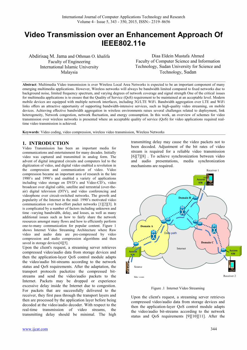
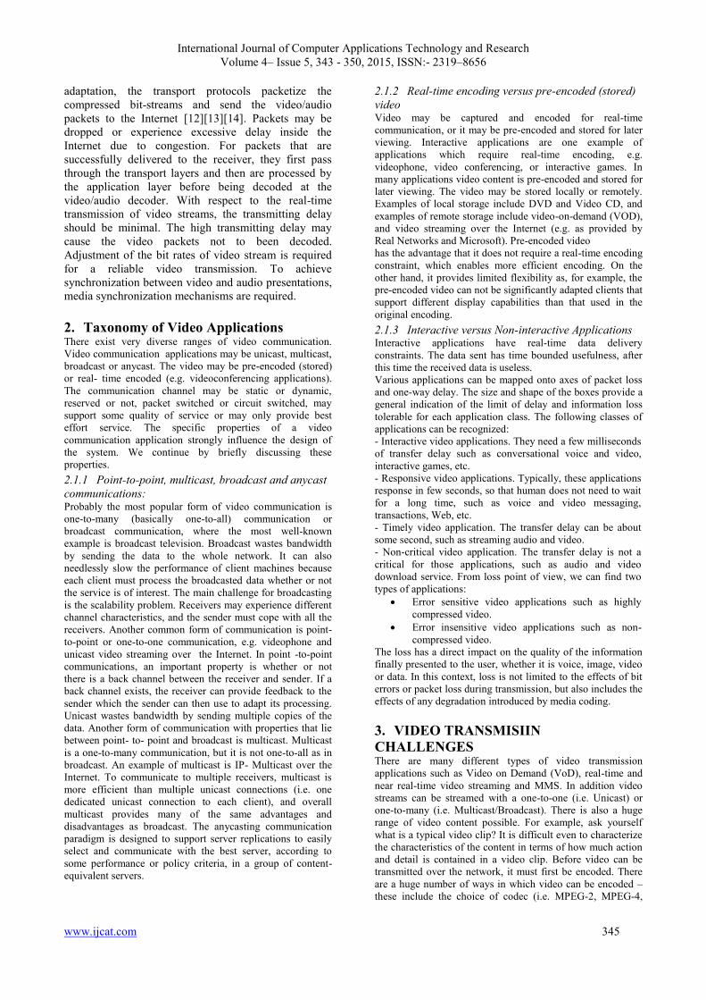
one-to-many communication for popular content. Figure 1
shows Internet Video Streaming Architecture where Raw
video and audio data are pre-compressed by video
compression and audio compression algorithms and then
saved in storage devices[4][5].
Upon the client's request, a streaming server retrieves
compressed video/audio data from storage devices and
then the application-layer QoS control module adapts
the video/audio bit-streams according to the network
status and QoS requirements. After the adaptation, the
transport protocols packetize the compressed bit-
streams and send the video/audio packets to the
Internet. Packets may be dropped or experience
excessive delay inside the Internet due to congestion.
For packets that are successfully delivered to the
receiver, they first pass through the transport layers and
then are processed by the application layer before being
decoded at the video/audio decoder. With respect to the
real-time transmission of video streams, the
transmitting delay should be minimal. The high
transmitting delay may cause the video packets not to
been decoded. Adjustment of the bit rates of video
stream is required for a reliable video transmission
[6][7][8] . To achieve synchronization between video
and audio presentations, media synchronization
mechanisms are required.
Figure .1 Internet Video Streaming
Upon the client's request, a streaming server retrieves
compressed video/audio data from storage devices and
then the application-layer QoS control module adapts
the video/audio bit-streams according to the network
status and QoS requirements [9][10][11]. After the
AAcccceessss SSWW
Data path
AAcccceessss SSWW
Domain A
Domain B
Domain C
Internet
AAcccceessss SSWW
Source
Receiver 2
Receiver 1
bbc.com
International Journal of Computer Applications Technology and Research
Volume 4– Issue 5, 343 - 350, 2015, ISSN:- 2319–8656
www.ijcat.com 345
adaptation, the transport protocols packetize the
compressed bit-streams and send the video/audio
packets to the Internet [12][13][14]. Packets may be
dropped or experience excessive delay inside the
Internet due to congestion. For packets that are
successfully delivered to the receiver, they first pass
through the transport layers and then are processed by
the application layer before being decoded at the
video/audio decoder. With respect to the real-time
transmission of video streams, the transmitting delay
should be minimal. The high transmitting delay may
cause the video packets not to been decoded.
Adjustment of the bit rates of video stream is required
for a reliable video transmission. To achieve
synchronization between video and audio presentations,
media synchronization mechanisms are required.
2. Taxonomy of Video Applications There exist very diverse ranges of video communication.
Video communication applications may be unicast, multicast,
broadcast or anycast. The video may be pre-encoded (stored)
or real- time encoded (e.g. videoconferencing applications).
The communication channel may be static or dynamic,
reserved or not, packet switched or circuit switched, may
support some quality of service or may only provide best
effort service. The specific properties of a video
communication application strongly influence the design of
the system. We continue by briefly discussing these
properties.
2.1.1 Point-to-point, multicast, broadcast and anycast
communications: Probably the most popular form of video communication is
one-to-many (basically one-to-all) communication or
broadcast communication, where the most well-known
example is broadcast television. Broadcast wastes bandwidth
by sending the data to the whole network. It can also
needlessly slow the performance of client machines because
each client must process the broadcasted data whether or not
the service is of interest. The main challenge for broadcasting
is the scalability problem. Receivers may experience different
channel characteristics, and the sender must cope with all the
receivers. Another common form of communication is point-
to-point or one-to-one communication, e.g. videophone and
unicast video streaming over the Internet. In point -to-point
communications, an important property is whether or not
there is a back channel between the receiver and sender. If a
back channel exists, the receiver can provide feedback to the
sender which the sender can then use to adapt its processing.
Unicast wastes bandwidth by sending multiple copies of the
data. Another form of communication with properties that lie
between point- to- point and broadcast is multicast. Multicast
is a one-to-many communication, but it is not one-to-all as in
broadcast. An example of multicast is IP- Multicast over the
Internet. To communicate to multiple receivers, multicast is
more efficient than multiple unicast connections (i.e. one
dedicated unicast connection to each client), and overall
multicast provides many of the same advantages and
disadvantages as broadcast. The anycasting communication
paradigm is designed to support server replications to easily
select and communicate with the best server, according to
some performance or policy criteria, in a group of content-
equivalent servers.
2.1.2 Real-time encoding versus pre-encoded (stored)
video Video may be captured and encoded for real-time
communication, or it may be pre-encoded and stored for later
viewing. Interactive applications are one example of
applications which require real-time encoding, e.g.
videophone, video conferencing, or interactive games. In
many applications video content is pre-encoded and stored for
later viewing. The video may be stored locally or remotely.
Examples of local storage include DVD and Video CD, and
examples of remote storage include video-on-demand (VOD),
and video streaming over the Internet (e.g. as provided by
Real Networks and Microsoft). Pre-encoded video
has the advantage that it does not require a real-time encoding
constraint, which enables more efficient encoding. On the
other hand, it provides limited flexibility as, for example, the
pre-encoded video can not be significantly adapted clients that
support different display capabilities than that used in the
original encoding.
2.1.3 Interactive versus Non-interactive Applications Interactive applications have real-time data delivery
constraints. The data sent has time bounded usefulness, after
this time the received data is useless.
Various applications can be mapped onto axes of packet loss
and one-way delay. The size and shape of the boxes provide a
general indication of the limit of delay and information loss
tolerable for each application class. The following classes of
applications can be recognized:
- Interactive video applications. They need a few milliseconds
of transfer delay such as conversational voice and video,
interactive games, etc.
- Responsive video applications. Typically, these applications
response in few seconds, so that human does not need to wait
for a long time, such as voice and video messaging,
transactions, Web, etc.
- Timely video application. The transfer delay can be about
some second, such as streaming audio and video.
- Non-critical video application. The transfer delay is not a
critical for those applications, such as audio and video
download service. From loss point of view, we can find two
types of applications:
Error sensitive video applications such as highly
compressed video.
Error insensitive video applications such as non-
compressed video.
The loss has a direct impact on the quality of the information
finally presented to the user, whether it is voice, image, video
or data. In this context, loss is not limited to the effects of bit
errors or packet loss during transmission, but also includes the
effects of any degradation introduced by media coding.
3. VIDEO TRANSMISIIN
CHALLENGES There are many different types of video transmission
applications such as Video on Demand (VoD), real-time and
near real-time video streaming and MMS. In addition video
streams can be streamed with a one-to-one (i.e. Unicast) or
one-to-many (i.e. Multicast/Broadcast). There is also a huge
range of video content possible. For example, ask yourself
what is a typical video clip? It is difficult even to characterize
the characteristics of the content in terms of how much action
and detail is contained in a video clip. Before video can be
transmitted over the network, it must first be encoded. There
are a huge number of ways in which video can be encoded –
these include the choice of codec (i.e. MPEG-2, MPEG-4,

International Journal of Computer Applications Technology and Research
Volume 4– Issue 5, 343 - 350, 2015, ISSN:- 2319–8656
www.ijcat.com 346
H.264, AVI, WMV etc.), the target bit rate, the frame rate,
equalization parameter, the resolution and so on. The choice
of these parameters will affect the delivery of the video on the
network. Once the video has been encoded, it is then
transmitted/streamed using a streaming server. The server can
transmit the video in a number of ways using various
transmission protocols and packetization schemes. The client
periodically sends feedback to the server telling the server
how much information has been received. The server uses this
feedback to adapt the transmitted video stream so as to
minimize the any negative effects of congestion in the
network might have on the video stream. The ability of the
server to optimally adapt the video stream depends on the
frequency of the feedback and the relevance, usefulness, and
accuracy of the feedback information [15][16]. There are a
number of different techniques that can be used in the server
to adapt the video quality including rate control, rate shaping,
frame dropping, and stream switching. Finally, to add to the
difficulties of video streaming, there are no accepted metrics
to calculate video quality so as to correlate to the Human
Visual System (HVS) or in other words human perception,
e.g. PSNR, VQM, MPQM, PVQ etc [6]. There is a strong
demand in modern societies for pioneering ICT services that
will support modern social infrastructures. Emerging new
techniques in the fields of wireless communication, network
coding and video transmission, which can be used as a base
for creating smart services that would serve people’s everyday
life in modern societies? Typical example of such services is
video surveillance over wireless networks to support traffic
monitoring, fire detection and real-time events (such as
natural disasters) broadcasting for the societies of the smart
cities , real time monitoring of patients in ICU.
4. VIDEO QUALITY EVALUATION Several factors, such as network delay, packet loss etc., may
lead to loss of video data that can distort the video sequence.
Two types of methodologies have become popular that can
measure the distortion: objective assessment and subjective
assessment. We describe these approaches in the following
text.
4.1 Objective Assessment Objective Assessment methods use algorithms to measure the
distortion in a given video sequence. These algorithms are fast
and very easy to use [17] . Most of these algorithms require
the original signal in order to compare it with the distorted
signal. One of the most popular methods is to use the Peak
Signal-to-Noise Ratio (PSNR) measure.
PSNR gives the distortion between the original and the
processed (impaired) versions of a video sequence. Let’s say
that we have two sequences: S (original) and S′ (impaired).
S(x, y, k) is the luminance of a pixel at position x, y in frame k
from the original sequence and S′(x, y, k) is the luminance of a
pixel at the corresponding position in the impaired version.
The sequences are K frames long, the frame size is M * N
pixels, and each pixel luminance is represented with 8 bits.
The Mean Square Error is first obtained with the Equation.1.
N
x
M
y
K
k
kyxSkyxSKMN
MSE1
2'
11
)],,(),,([1
(1)
The MSE is the cumulative squared error between
the original and the impaired images. A lower MSE means a
smaller error. The PSNR is then computed with the following
equation 2.:-
MSEPSNR
255log20 10 (2)
The unit of the PSNR is a decibel value (dB), 255 is
the maximum possible pixel value of the image. When the
pixels are represented using 8 bits per sample. Typical values
for the PSNR image and video compression are between 30
and 50 dB, where higher is better. Acceptable values for
PSNR are considered to be about 28 dB to 35 dB.
4.2 Subjective Assessment Subjective assessment methods are supposed to be the best
indicators of the video quality, for a video that will be watched
by humans, because the assessment is done by real humans. In
general a distorted sequence, in addition to the original
sequence, is shown to the human subjects and they are asked
to give a score to the sequence. Later, the scores from several
subjects are statistically processed to give a mean score (the
MOS or Mean Opinion Score) for that particular distorted
sequence.
The ITU-R Recommendation (ITU-R, 2002) defines
several standard methods and procedures for the subjective
quality assessment of television pictures. One of the methods
is called Double-Stimulus Impairment Scale (DSIS). In DSIS
method, an assessor is first presented with the original video
sequence, and then he is shown the distorted version. The
assessor rates the degree of the impairment of the second
image having the reference in mind. This is repeated with
several pairs of sequences. The score for each sequence is
taken from the impairment scale shown in Table 1.
Table 1 Impairment scale
Number
Score
Impairment Scale Quality of Scale
5 Imperceptible Excellent
4 Perceptible, but not
Annoying
Good
3 Slightly Annoying Fair
2 Annoying Poor
1 Very Annoying Unsatisfactory
5. CONTENT DELIVERY CHOICE
IMPLICATIONS Each delivery technique has some inherent advantages and
disadvantages. The selection of a means of delivery by
training and education organizations should be primarily based
on providing the best viewing experience to the learner as
possible for a given instructional design. Familiarity with the
various strengths and weaknesses of HTTP streaming, RTSP
streaming, and CD content distribution methods are essential
[18][19].
5.1 Streaming Quality Between HTTP and RTSP streaming techniques, HTTP
streaming usually permits content providers the ability to
provide higher data rates. These higher data delivery rates
permit higher quality files to be made available to viewers.
The disadvantage of having the ability to support higher data
delivery rates is the lengthy download times associated with
the files. Additionally, viewers must be willing to wait for
these files as well, often times needing a high-speed
connection to endure the longer download times [20][21][22].
The HTTP streaming method guarantees the
delivery of all of a given video files data, no matter how long
it takes. The implication is there will be no dropped frames or

International Journal of Computer Applications Technology and Research
Volume 4– Issue 5, 343 - 350, 2015, ISSN:- 2319–8656
www.ijcat.com 347
missing information data that will lead to picture quality
degradation. With RSTP streaming, there is no guarantee for
the complete delivery of data. Consequently, viewers may
experience dropped frames, excessive pixilation of images, or
“jerky” motions if the network cannot deliver all of the data on
time. If the network becomes overly congested, viewers may
be unable to view or hear all of the data intended for them.
However, with RSTP streaming, viewers will experience what
they do see at the intended time; similar to a broadcast.
Depending on the type of training and education being offered,
missing some of the data, some of the time, may become
unacceptable from a learning perspective.
For best picture quality, the CD or DVD will
provide the largest and richest quality pictures. Most of the
streaming methods are designed to deliver a smaller picture,
approximately 240 x 180, at 12 to 15 frames per second.
Because there is no network transfer involved with a CD or
DVD, picture quality can be as large as 720 x 480, at 30
frames per second. If picture quality of video multimedia is of
paramount importance in the instructional design of a given
the training and education module, then CDs and DVDs are
the delivery means of choice.
5.2 File Size and Performance For individual video files longer than five minutes, RTSP
streaming is usually a better choice than HTTP streaming.
When downloading larger files, HTTP streaming can present
problems for viewer connecting to the network without a high
speed connection. Additionally, those viewers lacking
adequate hard drive storage space and system processor speeds
on their local machines tend to be frustrated with HTTP
streaming architectures. Simply, the files take too long to
download and users become impatient waiting the video to
play. With RTSP streaming, there is only a small “priming”
file to download before the entire video file begins to play.
Under an RTSP streaming architecture, viewers can easily fast
forward ahead through a video file and only have to wait a few
seconds until the video playback begins to play at the new
start point. Such functionality is not possible with HTTP
streaming. With HTTP streaming, viewers cannot randomly
access portions of a particular clip without downloading the
entire file first.
Both types of streaming are suitable depending on
the instructional design of a given course. If the course is
supported by videos that are most likely to be watched once,
RTSP streaming is suitable. However, if it is anticipated that
students will watch the video repeatedly, viewing the file on a
CD or DVD will provide a more satisfying experience.
6. IEEE802.11E PERFORMANCE
ANALYSIS FOR VIDEO
TRANSMISSION
In this work, Networks were designed for non-real time traffic,
like data are today being used to support real-time applications
like Video streaming which are inherently different from data
traffic. Video applications have very different requirements
and characteristics compared to data traffic. Packet-loss affects
the quality of video and degrades the user experience. End-to-
end delay is also an important requirement, similar to that the
throughput and bandwidth requirement is important. The
traffic characteristics of the non-video flows were used in the
simulations. The non-video flows were chosen to provide a
mix of traffic types to compete in the medium & increase the
network load since all the stations share the access to the same
channel to evaluate the performance analysis.
In this Scenario, video is given higher priority that
the other video traffics; Hence, video gets faster access to the
medium.
Figure 2 shows the network topology used for the simulation
experiments of the first and second scenario which is a single
AP with thee traffic flows.
Figure 2 Three traffic flows
This scenario demonstrates three data flows. The
number of mobile stations was increased from 3 to 15 to
increase the network load. Three stations are added every
simulation and each one of them transmits different data flow
than others such as video, voice or best-effort data flow. This
scenario is to calculate the throughput, delay and packet loss
characteristics with the variation of number of stations.
For the second scenario is similar to the first one
except that the number of mobile stations was increased from
3 to 9, there are 3 groups of stations with 3 stations each. The
first group transmits video flow, while the second transmits
voice flow, and the third transmits best-effort data flow.
Relatively, delay and packet loss are calculated under the
variation of the topology where the stations are moving from
100 to 1000 square meters. This is considered as a very
difficult scenario and it may be used to design hotspots under
different conditions. Table 2 shows the IEEE802.11e MAC
parameters values used in the simulation for the two scenarios.
Table 2 IEEE802.11e MAC Parameters
Parameter
Value
Slot time 20 us
Beacon interval 100 ms
Fragmentation threshold 1024 Bytes
RTS threshold 500Bytes
SIFS 10 us
PIFS 40 us
DIFS 50 us
MSDU (Voice and Video) 60 ms
MSDU (data) 200 ms
Retry limit 7
TXOP limit 3428 us
CAP rate 21 us
CAP max 8000 us
CAP timer 5120 us

International Journal of Computer Applications Technology and Research
Volume 4– Issue 5, 343 - 350, 2015, ISSN:- 2319–8656
www.ijcat.com 348
The number of mobile stations is increased from 3 to
15 with 3 stations at a time to increase the network load. As
mentioned in the introduction of this simulation, every three
QoS stations transmit three different types of flows (video,
voice and best-effort data) to the same destination, which is
the access point, and the PHY data rate is set 11 Mbps. Table
3 shows the simulation parameters used in the first & second
scenario.
Table 3 Enhanced EDCA Simulation Parameters
Simulation
Parameter
Video Voice Best
effort
Transport Protocol UDP UDP UDP
CWmin 3 7 15
CWmax 7 15 1023
AIFSN 1 2 3
Packet Size (bytes) 1028 160 1500
Packet Interval (ms) 10 20 12.5
Data rate (kbps) 822.40 64 960
All the simulation results are averaged over five
simulations, with random starting time for each flow. There is
a variation in the channel load by increasing the number of
active QoS stations from 3 to 15 with 3 stations at a time. All
stations are in the range of each other.
Table 4 shows the original IEEE802.11e parameters
used in the first scenario & second scenario
Table 4 Original IEEE802.11e EDCA Simulation Parameters
Simulation
Parameter
Video Voice Best-effort
Data
CWmin 7 15 31
CWmax 15 31 1023
AIFSN 2 3 4
Results are based on the three basic performance
metrics (Throughput, delay and packet loss) for the different
access categories (video, voice and best-effort data). These
metrics were selected due to their great effect on the
IEEE802.11e performance for QoS support.
7. DEMONSTRATION RESULTS In this section, a few simulation results of the two scenarios
respectively as a comparative performance analysis of
IEEE802.11e WLAN protocol are presented. These results
include throughput, average end-to-end delay and packet loss.
It also provides a detailed explanation of the behaviour of
IEEE802.11e supported by graphs. The number of mobile
stations is increased from 3 to 15 with 3 stations at a time to
increase the network load. As mentioned in the introduction of
this simulation, every three QoS stations transmit three
different types of flows (video, voice and best-effort data) to
the same destination, which is the access point, and the PHY
data rate is set 11 Mbps. Table 4 shows the simulation
parameters used in this scenario.
Table 4 Enhanced EDCA Simulation Parameters
All the simulation results are averaged over five simulations,
with random starting time for each flow. There is a variation in
the channel load by increasing the number of active QoS
stations from 3 to 15 with 3 stations at a time. All stations are
in the range of each other. Table 5 shows the original
IEEE802.11e parameters used in this scenario.
Table 5 Original IEEE802.11e EDCA Simulation Parameters
for the first & second scenario
Simulation
Parameter
Video Voice Best-effort
Data
CWmin 7 15 31
CWmax 15 31 1023
AIFSN 2 3 4
Results are based on the three basic performance metrics
(Throughput, delay and packet loss) for the different access
categories (video, voice and best-effort data). These metrics
were selected due to their great effect on the IEEE802.11e
performance for QoS support. The following analysis focuses
the throughput results for the first scenario, which is shown in
Figure 3.
Number of Stations Vs Throughput
0
1
2
3
4
5
6
7
8
1 3 5 7 9 11 13 15
Number of Stations
Th
rou
gh
pu
t (M
bp
s)
Video[enhanced]
Voice[enhanced]
Best-Effort[enhanced]
Video[original]
Voice[original]
Best-Effort[original]
Figure 3 Effect of network load on throughput for different
access categories (video, voice and best effort data) using
original & enhanced EDCA values
Simulation
Parameter
Video Voice Best effort
Transport Protocol UDP UDP UDP
CWmin 3 7 15
CWmax 7 15 1023
AIFSN 1 2 3
Packet Size
(bytes)
1028 160 1500
Packet Interval
(ms)
10 20 12.5
Data rate (kbps) 822.40 64 960

International Journal of Computer Applications Technology and Research
Volume 4– Issue 5, 343 - 350, 2015, ISSN:- 2319–8656
www.ijcat.com 349
The graph illustrates the effect of increasing the number of
active QoS stations transmitting data to the access point on the
throughput values for the three data flows. The sending rate in
this simulation is 11 Mbps, while the CWmin and CWmax size
and AIFSN values as stated in Table 4 &5. In comparison,
Figure 3 illustrates the effect of increasing the number of
active QoS stations transmitting data to the access point on the
throughput values for the three data flows using IEEE802.11e
standard (IEEE, 2003) CW size and AIFSN values shown in
Table 5.
Enhanced CW size and AIFSN values provide better
results considering the video and voice flows, this is clearly
observed from Figure 3. In both cases, it is clearly seen from
the graphs that IEEE802.11e provides service differentiation
for different priorities when the system is heavily loaded by
increasing the number of stations. When the number of
stations is 3 or 6, all the data flows have equal channel
capacity. However, in the case of 9, 12, and 15 stations, the
channel is reserved for higher priority data flows. As
explained in the beginning of this chapter, video flow has the
highest priority among the others, while the best effort data
flow has the lowest priority.
The average end-to-end delay is another important
performance metric that should be taken into account. Figure 4
represent the results obtained from the simulations using the
enhanced CW size and AIFSN values.
Number of Nodes Vs Average end-to-end delay
0
100
200
300
400
500
600
700
800
1 3 5 7 9 11 13
Number of Nodes
Av
era
ge
en
d-t
o-e
nd
de
lay
(m
s)
Video [enhanced]
Voice [enhanced]
Best Effort [enhanced]
Video [original]
Voice [original]
Best Effort [original]
Figure 4 Effect of network load on the average end-to-end
delay for different access categories (voice, video and best
effort data) using original & enhanced EDCA values.
Figures 4 illustrate the effect of increasing the number of
active QoS stations transmitting data to the access point on the
average end-to-end delay values for the three data flows
separately from source (mobile stations) to destination (access
point). It was modified the first scenario so that all the stations
transmit three types of data flows. The channel load was
varied by increasing the number of active QoS stations from 1
to 14. The enhanced CW size and AIFSN values illustrates
better performance with respect to the video and voice flows,
but not for the best effort data flow. This is shown in Figure 5
when the active QoS stations are 11.
As comparison, Figure 6 similarly represents the
simulation results using the CW size and AIFSN values in
Table 5. These enhanced values provide better results than
ours with respect to best effort data flow. Here, the main
concern is to enhance the performance for Video flow.
Another important factor that has a great effect on
the IEEE802.11e WLAN performance for QoS support is the
packet drop and loss ratio. To calculate the number of packets
dropped or lost in the transmission medium, we subtract the
number of packet successfully received by the receiver (the
access point in our case) from the total number of packets sent
by the sender (mobile stations).
In Figure 5, illustrates the effect of increasing the
number of active QoS stations on the packet drop and loss
ratio. The network load was varied by 3 stations at a time
sending three different data flows. In this simulation, is to
compare the original with the enhanced IEEE802.11e
parameters.
It is clearly observed from Figure 6 the service
differentiation between the different data flows according to
their priority levels. This difference appears more when the
channel is heavily loaded by increasing the number of stations.
For the best effort data flow, the packet drop starts when the
number of stations is 3. That is due to the fact that best-effort
data flow has the lowest priority. On the other hand, as the
video flow is considered, the packet drop starts when the
number of stations increases to 9.
This reflects the fact that video flow has the highest
priority to reserve the channel when it is heavily loaded. The
percentage of the packet drop reaches up to 82% for the
maximum channel load considering the best effort data flow,
while it reaches up to 19% for the video flow.
Number of Stations Vs Packet Drop Ratio
0
10
20
30
40
50
60
70
80
90
100
1 3 5 7 9 11 13 15
Number of Stations
Pa
ck
et
Dro
p R
ati
o (
%)
Video[enhanced]
Voice[enhanced]
Best-
Effort[enhanced]
Video[original]
Voice[original]
Best-Effort[original]
Figure 5 Effect of number of stations on the Packet drop ratio
for different access categories (voice, video and best effort
data) using original & enhanced EDCA values.
In fact, the system throughput is inversely proportional to the
number of stations. And the number of stations is inversely
proportional to the dropped and lost packets. In addition,
packet drop has great effect on the network average end-to-
end delay. Delay is directly proportional to the number of
dropped packets.
8. CONCLUSION Video transmission over wireless networks and the internet is
a challenging task due to the stringent QoS required by video
applications and also affected by many channel impairments.
In this work, An Enhancement approaches of IEEE802.11e
were presented. Different simulation scenarios such as
average end-to-end delay, throughput and packet loss ratio to
suite different environments under various conditions in
performance analysis for MPEG-4 video transmission over
WLANs were conducted. The level of performance such as

International Journal of Computer Applications Technology and Research
Volume 4– Issue 5, 343 - 350, 2015, ISSN:- 2319–8656
www.ijcat.com 350
Packet loss, PSNR, Decodable Frame Rate (Q) were evaluated
which shows better results for lower packet loss, higher
Throughput, PSNR & Decodable Frame Rate (Q) for MPEG-
4 video transmission over IEEE802.11e. The experimentation
results have shown that MPEG-4 video streaming services
performs well only when the SNR is above 30dB. However,
the received video quality becomes unacceptable in 20 dB to
30 dB. Any traffic transmission will be easily denied when the
SNR is below 20dB.
REFERENCES [1] Vinod B Durdi, P. T. Kulkarni, and K. L. Sudha, Robust
Video Transmission over Wireless Networks Using
Cross Layer Approach” , Journal of Industrial and
Intelligent Information Vol. 1, No. 2, June 2013:
[2] Kalvein Rantelobo, Wirawan, G. Hendrantoro, A.
Affandi, and Hua-An Zhao, “A New Scheme for
Evaluating Video Transmission over Broadband
Wireless Network “ , Future Wireless Networks and
Information Systems, LNEE 143, pp. 335–341,
Springerlink.com © Springer-Verlag Berlin Heidelberg
2012
[3] S.M. Koli, R.G. Purandare, S.P. Kshirsagar, and V.V.
Gohokar, “A Survey on Video Transmission Using
Wireless Technology “,CCSIT 2011, Part II, CCIS 132,
pp. 137–147, Springer-Verlag Berlin Heidelberg 2011.
[4] Gopikrishnan.R , “An Efficient Real Time Video
Multicasting Protocol and WLANs Cross-Layer
Optimization in IEEE 802.11N “, IJCSMC, Vol. 3, Issue.
2, February 2014, pg.811 – 814
[5] S Kumar, Reactive and Proactive Routing Protocols for
Wireless Mesh Network using Multimedia
Streaming[A]. Proceedings of the International
Conference on Recent Advances and Future Trends in
Information Technology (iRAFIT 2012) (: International
Journal of Computer Applications, Special Issue[C],
2012.
[6] T. Kim, “Scalable video streaming over internet”, P h.D.
Thesis, School of Electrical and Computer Engineering,
Georgia Institute of Technology, Jan. 2005.
[7] D. Wu, Y. T. Hou, W. Zhu, Y.-Q. Zhang and J. M. Peha,
“Streaming video over the internet: Approaches and
directions,” IEEE Trans. Circuits Syst. Video Technol.,
vol. 11, pp. 282–300, Mar. 2001.
[8] G. Conklin, G. Greenbaum, K. Lillevold, A. Lippman
and Y. Reznik, “Video coding for streaming media
delivery on the Internet,” IEEE Trans. Circuits Syst.
Video Technol., vol. 11, pp. 269–281, Mar. 2001.
[9] J.G. Apostolopoulos, W. Tan and S.J. Wee “Video Str
eaming: Concepts, Algorithms, and Systems” Mobile
and Media Systems L aboratory HP Laboratories Palo
Alto, HPL-2002-260, Sept. 2002.
[10] F. Yang, Q. Zhang, W. Zhu and Y.Q. Zhang, “Bit Allo
cation for Scalable Video Streaming over Mobile
Wireless Internet”, Infocom, 2004.
[11] F. Ziliani and J-C. Michelou, “Scalable Video Codin g
in Digital Video Security”, White paper, VisioWave,
2005.
[12] Y.-M. Hsiao, J.-F. Lee, J.-S. Chen, and Y.-S. Chu,
“H.264 video transmissions over wireless networks:
challenges and solutions,” Computer Communications,
vol. 34, no. 14, pp. 1661–1672, 2011. View at Publisher
· View at Google Scholar · View at Scopus
[13] M. van der Schaar and N. S. Shankar, “Cross-layer
wireless multimedia transmission: challenges,
principles, and new paradigms,” IEEE Wireless
Communications, vol. 12, no. 4, pp. 50–58, 2005.
[14] Z. Han, G.-M. Su, A. Kwasinski, M. Wu, and K. J. R.
Liu, “Multiuser distortion management of layered video
over resource limited downlink multicode-CDMA,”
IEEE Transactions on Wireless Communications, vol. 5,
no. 11, pp. 3056–3067, 2006. View at Publisher · View
at Google Scholar · View at Scopus
[15] F. Fu and M. van der Schaar, “A systematic framework
for dynamically optimizing multi-user wireless video
transmission,” IEEE Journal on Selected Areas in
Communications, vol. 28, no. 3, pp. 308–320, 2010.
View at Publisher · View at Google Scholar · View at
Scopus
[16] F. Li, G. Liu, and L. He, “Cross-layer approach to
multiuser H.264 video transmission over wireless
networks,” Journal of Multimedia, vol. 5, no. 2, pp.
110–117, 2010. View at Publisher · View at Google
Scholar · View at Scopus
[17] D.-E. Meddour, A. Abdallah, T. Ahmed, and R.
Boutaba, “A cross layer architecture for multicast and
unicast video transmission in mobile broadband
networks,” Journal of Network and Computer
Applications, vol. 35, no. 5, pp. 1377–1391, 2012. View
at Publisher · View at Google Scholar · View at Scopus
[18] L. Superiori, M. Wrulich, P. Svoboda et al., “Content-
aware scheduling for video streaming over HSDPA
networks,” in Proceedings of the 2nd International
Workshop on Cross Layer Design (IWCLD '09), pp. 1–
5, Palma de Mallorca, Spain, June 2009. View at
Publisher · View at Google Scholar · View at Scopus
[19] A. Chan, H. Lundgren, and T. Salonidis, “Video-aware
rate adaptation for MIMO WLANs,” in Proceedings of
the 19th IEEE International Conference on Network
Protocols (ICNP '11), pp. 321–330, British Columbia,
Canada, October 2011. View at Publisher · View at
Google Scholar · View at Scopus
[20] J. Rexford, “Performance evaluation of smoothing
algorithms for transmitting prerecorded variable-bit-rate
video,” IEEE Transactions on Multimedia, vol. 1, no. 3,
pp. 302–312, 1999. View at Publisher · View at Google
Scholar · View at Scopus
[21] A. Khalek, C. Caramanis, and R. Heath, “Video-aware
MIMO precoding with packet prioritization and unequal
modulation,” in Proceedings of the 20th European
Signal Processing Conference (EUSIPCO '12), pp.
1905–1909, Bucharest, Romania, August 2012.
[22] Ronak Dak, Dharm and Naveen Choudhary, A
Technical Survey based on Secure Video Transmission
Techniques, International Journal of Computer
Applications.2014, Number 2, pp 19-23.

International Journal of Computer Applications Technology and Research
Volume 4– Issue 5, 351 - 354, 2015, ISSN:- 2319–8656
www.ijcat.com 351
Frequent Data Mining in Data Publishing for Privacy
Preservation
Sheikh Nargis Nasir
Matoshri COERC,
Nashik, India
Swati A. Bhawsar
Matoshri COERC,
Nashik, India
Abstract: Weighted frequent pattern mining is suggested to find out more important frequent pattern by considering different weights
of each item. Weighted Frequent Patterns are generated in weight ascending and frequency descending order by using prefix tree
structure. These generated weighted frequent patterns are applied to maximal frequent item set mining algorithm. Maximal frequent
pattern mining can reduces the number of frequent patterns and keep sufficient result information. In this paper, we proposed an efficient
algorithm to mine maximal weighted frequent pattern mining over data streams. A new efficient data structure i.e. prefix tree and
conditional tree structure is used to dynamically maintain the information of transactions. Here, three information mining strategies (i.e.
Incremental, Interactive and Maximal) are presented. The detail of the algorithms is also discussed. Our study has submitted an
application to the Electronic shop Market Basket Analysis. Experimental studies are performed to evaluate the good effectiveness of our
algorithm..
Keywords: Data Mining, Incremental mining, Interactive mining, Maximal mining, Support;
1. INTRODUCTION Nowadays, many commercial applications have their
data presented in the form of continuously transmitted stream,
namely data streams. In such environments, data is generated
at some end nodes or remote sites and received by a local
system (to be processed and stored) with continuous
transmission. It is usually desirable for decision makers to find
out valuable information hidden in the stream. Data-stream
mining [1][2] is just a technique to continuously discover useful
information or knowledge from a large amount of running data
elements. Apart from traditional databases, evolving data set
has some special properties: continuous, unbounded, coming
with high speed and time varying data distribution. Therefore,
discovering knowledge from data streams masquerades some
limitations as follows. First, traditional multi-scan algorithms
are no more allowed on infinite data as it can’t be stored.
Second, the algorithm must be as fast as possible because of
high arrival rate of the data; otherwise, the accuracy of mining
results will be decreased. Third, the data distribution within the
data streams should be kept to avoid concept drifting problem.
Fourth, it needs incremental processes to process the existing
data as less as possible.
On the other hand, the main problem exists in this
work is that the actual profits of items are not considered. In
many applications, such as e-business, this factor is often one
of the most important factors for the results. To triumph over
this problem, frequent pattern mining [3] emerges as a new
research issue for discovering the itemsets with high weights,
i.e., high profits. To discover useful information from data
streams, we need not only efficient one-pass algorithms but
also effective data summary techniques.
The remainder of this paper is organized as follows.
In section 2, we describe motivation. In section 3, we develop
our proposed technique weighted frequent pattern mining over
data stream. In section 4, our experimental results are presented
and analyzed. Lastly, in section 5, conclusions are drawn.
2. MOTIVATION In the very beginning some weighted frequent pattern
mining algorithms MINWAL [4], WARM [5], WAR[6] have
been developed based on the Apriori Algorithm [7]. There are
two main problems exist in relevant studies: (1) The utilities
(e.g., importance or profits or weights) of items are not
considered. Actual weights of patterns cannot be reflected in
frequent patterns. (2) Existing weighted frequent pattern
mining methods produce too many patterns and this makes it
difficult for the users to filter useful patterns among the huge
set of patterns. In examination of this, in this paper we proposed
a framework, to find maximal high utility patterns from data
streams.
Motivated by these real world scenarios, in this
paper, we propose a tree based technique to mine weighted
frequent patterns over data streams. It can discover useful
recent knowledge from a data stream by using a single scan.
Our technique exploits a tree growth mining approach to avoid
level-wise candidate generation and test problem. Besides retail
market data, our technique can be well applied for the area of
mining weighted patterns. By considering different importance
values for different items, our algorithm can discover very
important knowledge about weighted frequent items in real
time using only one scan of data stream. Downward closure
property is used to prune the infrequent patterns [7].
Main contributions of this paper are as follows: (1) This is the
first approach on mining the compact form of high utility
patterns from data streams; (2) the proposed framework is an
effective single-pass framework which meets the requirements
of data stream mining; (3) It also generates patterns which are
not only high utility but also maximal. This provides compact
and intuitive hidden information in the data streams. An itemset
is called maximal if it is not a subset of any other patterns [8].
3. TECHNIQUE USED: An evolving dataset may have infinite number of
transactions. A weighted support of pattern P is calculated over
by multiplying its support with its weight. Therefore, pattern P
is weighted frequent pattern if its weighted support is greater
than or equal to the minimum threshold. For example, if
minimum threshold is 3.0,”ab” is a weighted frequent pattern.
Its weighted support is 4*0.55=2.2, which is greater than the
minimum threshold. Let, X= (X1, X2, X3,....,Xm) Where, X is

International Journal of Computer Applications Technology and Research
Volume 4– Issue 5, 351 - 354, 2015, ISSN:- 2319–8656
www.ijcat.com 352
pattern of item set, X ϵ I and k ϵ [1,m]. The weight of pattern
(WT), P[X1,X2,X3,...,Xk] is given by:
Our proposed technique consist of some preliminary
steps like Generation of header table, Construction of tree
structure, Calculate weighted support, pattern pruning and
evaluation of maximal frequent patterns.
Initially, the database performs transactions
according to the user choice viz; get transaction or remove
transaction. Transactions are read one by one from a transaction
database and insert it into the tree according to any predefined
order. The header table gets updated according to weighted
ascending order and frequency descending order
simultaneously. Each entry in a header table explicitly
maintains item-id, frequency and weight information for each
item. Then, WFP mining takes into an account that generated
weighted frequent item sets. The generated weighted frequent
patterns are appended for the maximal weighted frequent
itemset mining. Then, Vertical bitmap is maintained to keep the
record of candidate patterns. It performs AND-ing operation on
the items of transactions. lastly, the final output is generated
from weighted frequent patterns i.e. Maximal weighted
frequent pattens mining. The proposed work is divided into
four major modules:
1. Database Transaction:
The weight of the items has to be taken into consideration so
that the algorithm can be more effective in real world
applications. The weight of the pattern is the average of the
weight of the itemsets that constitute the pattern if the weighted
support of the pattern is greater than or equal to the minimum
threshold. Header table is generated to handle the item weights
and frequency.
2. Calculate Weighted Support:
The value achieved when multiplying the support of a pattern
with the weight of the pattern is the weighted support of that
pattern. That is, given pattern P, the weighted support is defined
as WSupport(P) = Weight(P)*Support(P). A pattern is called a
weighted frequent pattern if the weighted support of the pattern
is no less than the minimum support threshold.
3. Pattern Pruning:
If the value of Weighted Support is greater than or equal to the
threshold, then it is considered as frequent pattern else pattern
is pruned.
4. Maximal Mining:
From the resultant weighted frequent patterns, maximal
weighted frequent patterns are extracted.
4. ALGORITHMIC STRATEGY: When new transactions are inserted or deleted, the
incremental algorithm is processed to update the discovered
most frequent itemsets. These transactions can be partitioned
into four parts according to whether they are high transaction-
weighted utilization itemsets or not in the original database.
Each part is then processed in its own procedure. A simple way
of finding possible frequent itemsets is to mine frequent
patterns from every possible transaction, and then calculate
weighted support of the occurrences of these patterns. The
details of the proposed incremental mining algorithm are
described below.
4.1.1 Algorithmic Strategy to Implement Incremental Data
Mining:
The important problem is extracting frequent item
sets from a large uncertain database. Frequent patterns are
interpreted by calculating the weighted support for each pattern
under the weight and frequency of the item. This issue is
technically challenging for an uncertain database which
contains an exponential number of possible patterns. By
observing that the mining process can be modeled as a Poisson
binomial distribution, we develop an approximate algorithm,
which can efficiently and accurately discover frequent item sets
in a large uncertain database. We also study the important issue
of maintaining the mining result for a database that is evolving
(e.g., by inserting a transaction). Specifically, we implement
incremental mining algorithms, which enable Probabilistic
Frequent Item set (PFI) results to be refreshed. This reduces the
need of re executing the whole mining algorithm on the new
database, which is often more expensive and unnecessary.
Downward Closure Property:
The downward closure property [1] is used to prune the
infrequent patterns. This property says that if a pattern is
infrequent, then all of its super patterns must be infrequent. We
can maintain the downward closure property by transaction
weighted utilization. In this method a data structure, called
prefix Tree, is introduced to maintain frequent item sets in
evolving databases. Another structure, called conditional,
arranges tree nodes in an order that is affected by changes in
weighted support for candidate pattern. The data structure is
used to support mining on a changing database. To our best
knowledge, maintaining frequent item sets in evolving
uncertain databases has not been examined before. Here, Static
Algorithms do not handle database changes. Hence, any change
in the database necessitates a complete execution of these
algorithms.
Following are the input and output requirements for
implementing this incremental data mining algorithm.
Input:
1. Database,
2. Weight Table,
3. Updated database,
4. Minimum threshold
Output:
1. Weighted Frequent Patterns
4.1.2 Algorithmic Strategy to Implement Interactive Data
Mining:
The data structures of the existing frequent pattern mining
algorithms do not have the "build once mine many" property.
As a consequence, they cannot use their previous data
structures and mining results for the new mining threshold.
This property means that by building the data structure only
once, several mining operations can be done for interactive
mining. For example, if the algorithms presented in the
previous works want to calculate which patterns cover 40% of
the total profit, then their internal data structures are designed
in such a way that they can only calculate the asked amount. If
the amount is changed from 40% to 30% of the total profit, then
they have to do the whole calculation from the very beginning.
They cannot take any advantage from their previous design.
They have shown that incremental prefix-tree structures are
quite possible and efficient using currently available memory
in the gigabyte range. In our real world, however, the users
need to repeatedly change the minimum threshold for useful
information extraction according to their application
requirements. Therefore, the "build once mine many" property
is essentially needed to solve these interactive mining
problems.

International Journal of Computer Applications Technology and Research
Volume 4– Issue 5, 351 - 354, 2015, ISSN:- 2319–8656
www.ijcat.com 353
Motivated by these real world scenarios, in this project, we
presented a tree structure, called frequent pattern tree (or high
utility stream tree) and an algorithm, called high utility pattern
mining over stream data, for incremental and interactive
weighted frequent pattern mining over data streams. By
exploiting a pattern growth approach, this algorithm can
successfully mine all the resultant patterns. Therefore, it can
avoid the level-wise candidate generation-and-test problem
completely and reduces a large number of candidate patterns.
As a consequence, it significantly reduces the execution time
and memory usage for stream data processing.
Input:
1. Database,
2. Weight Table,
3. Updated database,
4. Minimum threshold
Output:
1. Weighted Frequent Patterns
4.1.3 Algorithmic Strategy to Implement Maximal
Weighted Frequent Pattern Mining: In this Maximal Miner algorithm, a descending
support or frequency count order method is used. A divide-and-
conquer traversal paradigm is used to mine weighted FP-tree
for mining closed weighted patterns in bottom-up manner. The
Maximal frequent itemset tree is used to store so far found
(global) maximal weighted frequent patterns. After mining the
traversal transaction, the set of real maximal weighted frequent
Patterns is generated. This is because weighted Maximal
Mining carries out the maximal frequent pattern mining with
weight constraints. This proposed approach can reduces search
space effectively. As compared to other methods, FPmax
method only does the maximal frequent pattern mining without
weight constraints, its search space is larger than that of our
algorithm. Following diagram shows the location maximal
frequent itemsets in frequent itemsets and closed patterns.
In this algorithm, we use divide-and-conquer
paradigm with a bottom-up pattern-growth method and
incorporates the closure property with weight constrain to
reduce effectively search space. This also includes anti-
monotone property. The reason for that is weighted Maximal
Mining has a weight constraint to reduce the search space than
FPmax [27] which has not weight constraint. To reduce the
calculation time, they have used bit vectors and TID-lists for
each distinct item. But these lists become very large and
inefficient when the numbers of distinct items and/or
transactions become large.
Anti-monotone Property:
The main focus in weighted frequent pattern mining
is on satisfying the anti-monotone property[27] since this
property is generally broken when different weights are applied
to different items. Even if a pattern is weighted as infrequent,
its super patterns can be weighted as frequent since super
patterns of a low weight pattern can receive a high weight after
other items with higher weight are added.
Input:
1. Weight Table,
2. Frequent Patterns,
3. Minimum Threshold.
Output:
1. Maximal Weighted Frequent Patterns.
4.1.4 Mining Process:
Here, we develop scalable algorithms for finding frequent item
sets (i.e., sets of attribute values that appear together frequently
in tuples) for uncertain databases. Our algorithms can be
applied to tuple or transactions uncertainty models. Here, every
tuple or transaction is associated with a probability to indicate
whether it exists. The frequent item sets discovered from
uncertain data are naturally probabilistic, in order to reflect the
confidence placed on the mining results.
5. EXPERIMENTAL RESULTS:
5.1 Experimental Environment &
Datasets: Experimentation is carried out on Customer purchase
behaviors-supermarket basket databases. This synthetic dataset
contain statistical information for predicting what a customer
will buy in the future. The weight value associated with each
item represents the chance that a customer may buy that item
in the near future. These probability values may be obtained by
analyzing the users' browsing histories. For instance, if
customer visited the marketplace 10 times in the previous
week, out of which video products were clicked five times, the
marketplace may conclude that customer has a 50 percent
chance of buying videos. Conceptually, a database is viewed as
a set of deterministic instances (called possible patterns), each
of which contains a set of items. To implement and test this
system, we have used a market basket analysis- synthetic
dataset in which various transactions are performed on the
items of the market.
5.1.1 Observations of the system on sparse dataset: Impact of Parameter Minimum Threshold (delta)
Following graph in the figure 5.1 is drawn by taking different
minimum threshold values to the 15 number of transactions.
Analysis:
1. Time required by itemsets in frequency descending
order is less than the time consumed by itemsets in
weight ascending order.
2. As the threshold value increases, the run time
required is decreases.
Figure 5.1 Impact of the No. of Transactions
Observations:
To observe the behavior of our proposed system
under increased number of transactions, we applied a constant
threshold value i.e. Threshold value = 40. Following graph is
drawn from different number of transactions to the same input
value, runtime is calculated. Figure 5.2: Impact of No. of
transactions on efficiency
Analysis:
1. For any number of transactions, time required by the
structure in weight ascending order is greater than the structure
in frequency descending order.
2. As the number of transactions increases, the time required to
execute transactions also increases.

International Journal of Computer Applications Technology and Research
Volume 4– Issue 5, 351 - 354, 2015, ISSN:- 2319–8656
www.ijcat.com 354
Figure 5.2 Impact of Modified Transactions
5.1.2 Comparison between Sorting Frequency in
Descending Order and Weight in Ascending Order: Analysis from Graph 1 and Graph 2:
1. IWFPTFD guarantees that non candidate item can't be passed
in to the set of candidate patterns.
2. IWFPTFD creates tree structure from the candidate items
generated from IWFPTWA. hence, speed up the tree creation
process.
3. IWFPTED reduces memory space required to store items.
4. This speed up the overall time required to mine patterns.
Analysis:
1. When the newly discovered transactions are added to the
existing dataset, existing tree structure in modified for the
newly evolved transactions.
2. This reduces the processing overhead of the transactions.
Worst Case Scenario: When all the transactions are modified.
Best Case Scenario: When no transaction is modified.
6. CONCLUSION The algorithm exploits two tree structures which
employs weighted frequent pattern mining over data streams.
The major objective of discovering recent weighted frequent
patterns from uncertain database is fulfilled. By making use of
efficient tree structure, our projected technique could capture
newest data from a data stream. Since, it requires a single-pass
of data stream for tree construction and mining operations. It is
reasonably appropriate to apply maximal weighted frequent
pattern mining algorithm to the operational database. The
mining paradigm also prunes the unimportant patterns and
reduces the size of the search space. We executed this work on
synthetic dataset of Market Basket Analysis. The results show
that our paradigm reduces the size required to search a
frequently used patterns. Also, this could speed up the process
to mine weighted frequent patterns.
7. REFERENCES [1] Bifet, A., Holmes, G., Pfahringer, B., & Gavaldà, R.
(2011). Mining frequent closed graphs on evolving
data streams. In Proceedings of the 17th ACM
SIGKDD conference on Knowledge Discovery and
Data Mining (KDD 2011), San Diego, CA, USA (pp.
591–599).
[2] Cheng, J., Ke, Y., & Ng, W. (2008). A survey on
algorithms for mining frequent itemsets over data
streams. Knowledge and Information Systems,
16(1), 1–27.
[3] Agrawal, R., & Srikant, R. (1994). Fast algorithms
for mining association rules. In Proceedings of the
20th international conference on very large data
bases (pp. 487– 499).
[4] C. H. Cai, A.W. fu, C. H. Cheng and W. W.
Kwong,”mining association rules with weighted
items”.Proc of int. database engineering and
application symposiums, IDEAS 98,pp 68-7,Cardiff,
Wales, UK, 1998.
[5] F. Tao,”Weighted association rules using weighted
support and significant framework”, Proc. Ninth
ACM SIGKDD Int. conference on knowledge
discovery and data mining,pp 661-666, 2003.
[6] W. Wang and J. Yang and P.S. Yu,”WAR: Weighted
association rules for item intensities”, Knowledge
Information and Systems , vol 6, pp 203-229, 2004.
[7] Agrawal, R., Imielin´ ski, T., Swami, A. (1993).
Mining association rules between sets of items in
large databases. In Proceedings of the 12th ACM
SIGMOD international conference on management
of data, May (pp. 207–216).
[8] Gouda, K., & Zaki, M. J. (2001). Efficiently mining
maximal frequent itemsets. In Proceedings of the
IEEE international conference on data mining
(ICDM), San Jose (pp. 163–170).

International Journal of Computer Applications Technology and Research
Volume 4– Issue 5, 355 - 358, 2015, ISSN:- 2319–8656
www.ijcat.com 355
Test-Case Optimization Using Genetic and Tabu Search Algorithm in Structural Testing
Tina Belinda Miranda M. Dhivya K. Sathyamoorthy
Department of Computer Department of Computer Department of Computer
Science and Engineering Science and Engineering Science and Engineering
Panimalar Institute of Panimalar Institute of Panimalar Institute of
Technology, Chennai, India Technology, Chennai, India Technology, Chennai, India
Abstract-- Software test-case generation is the process of identifying a set of test cases. It is necessary to generate the test sequence
that satisfies the testing criteria. For solving this kind of difficult problem there were a lot of research works, which have been done
in the past. The length of the test sequence plays an important role in software testing. The length of test sequence decides whether
the sufficient testing is carried or not. Many existing test sequence generation techniques uses genetic algorithm for test-case
generation in software testing. The Genetic Algorithm (GA) is an optimization heuristic technique that is implemented through
evolution and fitness function. It generates new test cases from the existing test sequence. Further to improve the existing
techniques, a new technique is proposed in this paper which combines the tabu search algorithm and the genetic algorithm. The
hybrid technique combines the strength of the two meta-heuristic methods and produces efficient test- case sequence.
Keywords: Test sequence, testing criteria, test case generation, genetic algorithm, tabu search algorithm.
1. INTRODUCTION Software engineering is a discipline concerned
with all aspects of software right from development to its retirement.[18] Software testing plays a prime role in software development life cycle[7]. It is aimed at discovering the faults in software to provide software quality. In white box testing it is necessary to design a set of test cases that satisfy testing criteria[9]. A test case executes software with a set of input values and then compares the expected output with the obtained output to see whether the test has passed or failed. In this paper we focus on branch coverage. As software testing consumes about 50% of software development effort, test data generation plays an important role[8].
Various approaches for test data generations have
been developed. These can be classified into three broad categories: random, static and dynamic techniques. Some of the dynamic methods of test data generation using meta-heuristic techniques treat testing problem as search space or optimization problem. Due to the difficulty and complexity in the testing process, these techniques have to search a large space. Some of the meta-heuristic techniques
suffer from the problems of local optimum, when software testing is done.
The solution that is best within neighboring space and not globally is local optimal solution. The search algorithms have a tendency to converge immaturely to local optimum. Because of this, test data generated will not satisfy the testing criteria. Particularly, Genetic algorithm has problems like slow convergence, blind search and risk of getting stuck into local optimum solution.
This paper analyzes test-sequence generation
technique based on genetic and tabu search algorithms. Genetic algorithm generates new test data from previously generated good candidates. The tabu search is added to the mutation step of genetic algorithm to reduce the time of search.
The rest of this paper is organized as follows: The Section 2 deals with the related work. The Section 3 deals with the search algorithm. The Section 4 deals with the proposed solution. Section 5 deals with the experimental validation. The section 6 deals with the conclusion.
2. RELATED WORK
There are many search based meta heuristic
algorithms that have been proposed to generate the test
data. The main characteristic of meta heuristics is to find better solutions at each step by adjusting the sub solutions. Genetic algorithm is an important population-based algorithm. The way in which genetic algorithm was applied to testing the object-oriented software was done by
Tonella[4]. A population of test sequences was evolved using evolutionary techniques. The main disadvantage of the paper was that in case of complex conditions in the code the evolutionary search was reduced to random search. Later many researchers used the genetic algorithm for test data generation. Ahmed used the genetic algorithm
to generate the test data when path coverage was used as the test criteria[1]. This method covered more paths in one run thus improving structural coverage. The basic concepts of tabu search algorithm were explained by Glover [2]. The main concept of Tabu search to reduce the cost by providing maximum structural coverage. Many researchers used the tabu search algorithm for lot scheduling problems.

International Journal of Computer Applications Technology and Research
Volume 4– Issue 5, 355 - 358, 2015, ISSN:- 2319–8656
www.ijcat.com 356
3. SEARCH ALGORITHM There are several search algorithms. A search
algorithm will not find a global optima in a fair amount of time. Therefore, it is common to put premature stopping criteria based on the available computational resources. In this paper two search algorithms are analyzed.
Genetic Algorithm:
Genetic algorithm is a famous meta-heuristic search based algorithm [10]. It has been demonstrated that
the test cases generated by genetic algorithm are more efficient than the random search algorithm. Genetic
algorithm generates new test data from already generated good candidates. This algorithm is inspired by Darwin’s
Theory. The algorithm uses evaluation, selection, crossover
point and the mutation operators to generate new test cases
from the existing test sequence. The evaluation procedure measures the fitness of each individual solution also known
as chromosome in the population and assigns a value based on the optimizing criterion. The selection procedure selects
individuals randomly in the current population for
development of the next generation. The selection procedure chooses the individual solutions to be
recombined and mutated out of the initial population. Recombination procedure reproduces the selected
individuals and exchanges the information for generating new individuals. The information that is exchanged is
called crossover. The crossover procedure chooses the two selected individuals and then combines them, thereby
creating two new individuals. Mutation creates a small change to newly created individual. The resulting
individuals are then evaluated through the fitness function. The fitness procedure measures how well chromosome
satisfies the testing criteria. These concepts have been explained earlier in[5,6].
There is an issue in using the genetic algorithm
for generation of test cases because it suffers from problems like slow convergence, blind search and the risk of getting stuck to the local optimum solution. Local optimum is a solution that is best within the neighboring space but not globally.
Tabu Search Algorithm:
Tabu search is a meta heuristic approach which is used to solve the optimization problems[2,3]. It is designed in such a way to guide other methods to move away from the local optima. It provides memory to avoid falling into the local optima.
The main characteristics of Tabu Search are its
flexible memory structure which is designed so that criteria as well the information regarding the search are exploited thoroughly. Tabu maintains two different types of memory a short term memory and the long term memory. The recent moves are captured in the short term memory and the related moves are captured in the long term memory. The
intensification and the diversification strategies help the search process to give optimal results. The intensification strategies help to reinforce previous solutions that are found good. And the diversification strategies help to search new areas that have not been explored earlier. To avoid getting stuck in the local optima or searching the same solution, a
list is created to maintain the most recently visited solutions. This list is called as the tabu list. The tabu list consists of a set of forbidden moves to prevent cycling and avoids getting stuck to the local optima. The tabu search will search for better solutions until the testing criteria are met.
Choose population N uniformly at random from S(l)
While global optimum not found Copy best a solutions from N to N’ While N’ is not completely filled
Select 2 parents from N according to selection criterion Generate two offspring that are same as their parents Apply crossover on offspring Mutate each offspring Copy the 2 new offspring into N’ N=N’.
Create an intial solution n While the stopping criteria is not met
Create a set of solutions K that are the neighbors of n and that are not in
tabu list Choose a best solution n* in K Update the tabu list based on n* Let n=n*
End
Pseudo code of Genetic Algorithm
Pseudo code for Tabu Search Algorithm

International Journal of Computer Applications Technology and Research
Volume 4– Issue 5, 355 - 358, 2015, ISSN:- 2319–8656
www.ijcat.com 357
4. PROPOSED SOLUTION
A test suite is used to test the software. There is
an issue in selecting the appropriate test cases for testing. The inappropriate and redundant test case selection will increase the test sequence length. The genetic algorithm suffers from local optima, in order to avoid this situation; The hybrid algorithm is proposed which is a combination of the genetic algorithm and the tabu search algorithm. The tabu search algorithm is added to the mutation step of genetic algorithm to reduce the randomness and the execution time of search and this enhances the quality of the end result. The genetic algorithm is used initially and its result is passed to the tabu search algorithm and this deals with repeated individuals by forbidding it from being chosen. This helps in generating new individuals in the next generation which is not present in the tabu list.
Initially a group of test cases are generated. Then a set of test cases are selected randomly. The selected test cases are set as the population size. Recursively select a number of best solutions from the population size. Then select two parent test cases according to the selection criteria. Generate two offspring that are the replica of their parents. Use crossover on the offspring with specified probability. Then mutate the offspring based on the long term and short term tabu list in order to avoid the unwanted new offspring generation. Then generate new offspring and put into the solution. This gives the optimized test sequence.
5. EXPERIMENTAL VALIDATION
To evaluate the performance of this algorithm an
experiment was conducted to analyze the test suite. Initially a sample voter validation form was created and then structural testing had to be done. So, a set test cases were generated for the form. Then the genetic algorithm was used to optimize the test cases.
There after the same experiment was carried out using the proposed hybrid algorithm and similarly the test cases were optimized . And then by comparing the test cases produced by genetic algorithm and hybrid algorithm it was found that test cases produced by the hybrid algorithm was more efficient than the test cases produced by the genetic algorithm.
Fig.1. Test Suite size versus Optimized Test Suite Size
1. Generate Random Test cases and set
population size
2. Define the Initial Population Size called
PopSize
3. Generate the Random Population Set to
represent the possible test sequences
Define Fitness Function called Maximum
Coverage
4. For i=1 to MaxIterations
[Repeat Steps 6 to 10]
5. Select two Random Parents called P1 and P2
from Population Set
6. Perform crossover to generate new Child
7. Perform Mutation Operation Child=Mutation
(Child) using tabu search list
8. Population=Population U Child
9. Return Optimized Test Sequence
Fig.2.Time Duration versus Code Coverage
Algorithm for Hybrid Technique
International Journal of Computer Applications Technology and Research
Volume 4– Issue 5, 355 - 358, 2015, ISSN:- 2319–8656
www.ijcat.com 358
6. CONCLUSION In this paper we have the analyzed the way in
which the genetic algorithm and the tabu search algorithm are used for optimizing the test cases.
The disadvantages of the genetic algorithm are analyzed, the problem of getting stuck in the local optima are overcome by using the hybrid algorithm. The Hybrid algorithm proposed in this paper generates the test cases that satisfies the given test criteria. The results of optimized test case and statistical data support claim that this algorithm performs better than other related strategies. 7. REFERENCES
[1] Ahmed, M.A. and I. Hermadi, "GA-based multiple
paths test data generator," Computers and Operations Research, 2008. 35(10): p. 3107-3124.
[2] F. Glover and M. Laguna, “Tabu Search,”
Kluwer Academic Publishers, 1997.
[3] F. Glover, “Tabu Search Part I,” ORSA Journal on
Computing, Vol. 1, No. 3, 1989, pp. 190-206.
[4] Tonella, P, "Evolutionary testing of classes," ACM SIGSOFT Software Engineering Notes.Boston, MA, United states: Association for Computing Machinery, p.119-128, 2004.
[5] B Jones et al. “Automatic Structural Testing Using
Genetic Algorithms”, Software Engineering Journal, Vol.11, No.5, 1996.
[6] P McMinn, “Search-Based Software Test
Data Generation: A Survey”, Software
Testing, Verification and Reliability, Vol.14, No.2, pp. 105—156, 2004.
[7] I. Sommerville, “Software Engineering, Pearson
Education,”7th Edition, Tata Mc-Graw Hill, India, 2005.
[8] B. Beizer, “Software Testing Techniques,”
2nd Edition,van Nostrand Reinhold, New York, 1990.
[9] G. Myers. The Art of Software Testing. Wiley, New York, 1979.
[10] M. Harman, S.A. Mansouri, and Y. Zhang,“Search Based Software
Engineering: A Comprehensive Analysis and Review
Of Trends Techniques and Applications,”Technical Report
TR-09-03, King’s College, 2009.

International Journal of Computer Applications Technology and Research
Volume 4– Issue 5, 359 - 367, 2015, ISSN:- 2319–8656
www.ijcat.com 359
Object Oriented Software Testability (OOST) Metrics
Analysis
Pushpa R. Suri
Department of Computer Science and
Applications, Kurukshetra University,
Kurukshetra -136119, Haryana, India
Harsha Singhani
Institute of Information Technology &
Management (GGSIPU), Janak Puri, New
Delhi -110058, India
Abstract: One of the core quality assurance feature which combines fault prevention and fault detection, is often known as
testability approach also. There are many assessment techniques and quantification method evolved for software testability
prediction which actually identifies testability weakness or factors to further help reduce test effort. This paper examines all
those measurement techniques that are being proposed for software testability assessment at various phases of object oriented
software development life cycle. The aim is to find the best metrics suit for software quality improvisation through software
testability support. The ultimate objective is to establish the ground work for finding ways reduce the testing effort by
improvising software testability and its assessment using well planned guidelines for object-oriented software development
with the help of suitable metrics.
Keywords: Software Testability, Testability Metrics, Object Oriented Software Analysis, OO Metrics
1. INTRODUCTION
The testing phase of the software life-cycle is extremely cost
intensive 40% or more of entire resources from designing
through implementation to maintenance are often spent on
testing[1].This is due to the enlargement of software scale and
complexity, leading to increasing testing problems. A major
means to solve these problems is making testing easier or
efficient by improving the software testability. Software
testability analysis can help developing a more test friendly
testable applications. Software testability analysis helps in
quantifying testability value. Test designers can use this value
to calculate the test cases number that is needed for a complete
testing [2]. Software designers can use these values to compare
different software components testability, find out the software
weakness and improve it and project managers can use the
value to judge the software quality, determine when to stop
testing and release a program[3].
The purpose of this paper is to examine the software testability
measurement metrics at various stages of software
development life cycle in object oriented system. The study is
done to analyze various OO metrics related to testability and
study the literature for various other techniques and metrics for
evaluation of testability at design and analysis phase as well as
at coding and implementation phase respectively. The study is
done because metrics are a good driver for the investigation of
aspects of software. The evaluation of these metrics has direct
or indirect impact on the testing effort and thus, it affects
testability. So, by this study we would be able to serve two
objectives: (1) Provide practitioners with information on the
available metrics for Object Oriented Software Testability, if
they are empirically validated (from the point of view of the
practitioners, one of the most important aspects of interest, i.e.,
if the metrics are really fruitful in practice), (2) Provide
researchers with an overview of the current state of metrics for
object oriented software testability (OOST) from Design to
Implementation phase, focusing on the strengths and
weaknesses of each existing proposal. Thus, researchers can
have a broad insight into the work already done.
Another aim of this work is to help reveal areas of research
either lacking completion or yet to undertaken. This work is
organised as follows: After giving a brief overview of software
testability in section 2, the existing proposals of OO metrics
that can be applied to OO software presented is in Section 3.
Section 4 presents an overall analysis of all the proposals.
Finally, Section 5 presents some concluding remarks and
highlights the future trends in the field of metrics for object
oriented software testability.
2. SOFTWARE TESTABILITY
Software Testability as defined by IEEE standards [4] as: “(1)
Degree to which a system or component facilitates the
establishment of test criteria and the performance of tests to
determine whether those criteria have been met. (2) The degree
to which a requirement is stated in terms that permit
establishment of test criteria and the performance of tests to
determine whether those criteria have been met.”
Thus, Testability actually acts as a software support
characteristic for making it easier to test. As stated by Binder
and Freedman a Testable Software is one that can be tested
easily, systematically and externally at the user interface level
without any ad-hoc measure [5][6]. Whereas [2] describe it as
complimentary support to software testing by easing down the
method of finding faults within the system by focussing more
on areas that most likely to deliver these faults. The insight
provided by testability at designing, coding and testing phase is
very useful as this additional information helps in product

International Journal of Computer Applications Technology and Research
Volume 4– Issue 5, 359 - 367, 2015, ISSN:- 2319–8656
www.ijcat.com 360
quality and reliability improvisation [7][8]. All this has lead to
a notion amongst practitioners that testability should be
planned early in the design phase though not necessarily so. As
seen by experts like Binder it involves factors like
controllability and observability i.e. ability to control software
input and state along with possibility to observe the output and
state changes that occur in software. So, overall testable
software has to be controllable and observable[5].But over the
years more such quality factors like understandability,
traceability, complexity and test–support capability have
contributed to testability of a system[3].All these factors make
testability a core quality factor.
Hence, over the years Testability has been diagnosed as one of
the core quality indicators, which leads to improvisation of test
process. Several approaches as Program Based , Model Based
and Dependability Testability assessment for Testability
estimation have been proposed [9]. The studies mostly revolve
around the measurement methods or factors affecting
testability. We would take this study further keeping focus on
mainly object oriented system. As object oriented technology
has become most widely accepted concept by software industry
nowadays. But testability still is a taboo concept not used much
amongst industry mainly due to lack of standardization, which
may not be imposed for mandatory usage but just been looked
upon for test support[10].
3. SIGNIFICANT OBJECT
ORIENTED METRICS USED FOR
TESTABILITY ASSESSMENT
Over the years a lot of OO design and coding metrics have been
adopted or discussed by research practitioners for studying to
be relevantly adopted in quantification of software testability.
Most of these metrics are proposed by Chidamber and Kemerer
[11], which is found to be easily understandable and applicable
set of metrics suite. But along with that there are other metrics
suites also available such as MOOD metrics suite [12].These
metrics can be categorized as one of the following object
oriented characteristic metrics- Size, Encapsulation,
Polymorphism, Coupling, Cohesion, Inheritance and
Complexity. Along with that from testability perspective,
which is the main motive of study, we have discussed few
important UML diagram metric suite too. So, now we present
those OO metrics selected for consideration and that may best
demonstrate the present-day context of metrics for OOST:
I. CK Metrics Suite [11],[1]
CK Metrics suite contains six metrics, which are
indicative of object oriented design principle usage
and implementation in software.
i. Number of Children (NOC): It is a basic
size metrics which calculates the no of
immediate descendants of the class. It is an
inheritance metrics, indicative of level of
reuse in an application. High NOC
represents a class with more children and
hence more responsibilities.
ii. Weighted Method per class (WMC):
WMC is a complexity metrics used for
class complexity calculation. Any
complexity measurement method can be
used for WMC calculation most popular
amongst all is cyclomatic complexity
method[13]. WMC values are indicators of
required effort to maintain a particular
class. Lesser the WMC value better will be
the class.
iii. Depth of Inheritance Tree (DIT): DIT is
an inheritance metrics whose measurement
finds the level of inheritance of a class in
system design. It is the length of maximum
path from the node to the root of the
hierarchy tree. It is a helps in
understanding behaviour of class,
measuring complexity of design and
potential reuse also.
iv. Coupling between Objects (CBO): This is
a coupling metrics which gives count of no
of other classes coupled to a class, which
method of one class using method or
attribute of other class. The high CBO
indicates more coupling and hence less
reusability.
v. Lack of Cohesion Metrics (LCOM): It is
a cohesion metrics which measures count
of methods pairs with zero similarity minus
method pairs with non zero similarity.
Higher cohesion values lead too complex
class bringing cohesion down. So,
practitioners keep cohesion high by
keeping LCOM low. LCOM was later
reformed as LCOM* by Henderson-Sellers
[14] and used in few researches.
vi. Response for a class (RFC): RFC is the
count of methods implemented within a
class. Higher RFC value indicates more
complex design and less understandability.
Whereas, lower RFC is a sign of greater
polymorphism. Hence, it is generally
categorized as complexity metrics.
II. HS Metric Suite[14]
i. Line of Code (LOC) or Line of Code per
Class (LOCC): It is a size metrics which
gives total no of lines of code (non
comment & non blank) in a class.
i. Number of Classes (NC / NOC): The total
number of classes.
ii. Number of Attributes (NA / NOA): The
total number of attributes.
ii. Number of Methods (NM / NOM): The
total number of methods
iii. Data Abstraction Coupling (DAC): The
DAC measures the coupling complexity
caused by Abstract Data Types (ADTs)

International Journal of Computer Applications Technology and Research
Volume 4– Issue 5, 359 - 367, 2015, ISSN:- 2319–8656
www.ijcat.com 361
iv. Message Passing Coupling (MPC): number of send statements defined in a
class
v. Number of Overriden Methods (NMO):
defined as number of methods overridden
by a subclass.
III. MOOD Metrics Suite [12][1]
Metrics for object oriented design (MOOD) metrics
suite consists of encapsulation (MHF, AHF),
inheritance (MIF, AIF), polymorphism (POF) and
coupling metrics (COF). This model was based on
two major features of object oriented classes i.e.
methods and attributes. Each feature is either hidden
or visible from a given class. Each metrics thus
calculates values between lowest (0%)-highest
(100%) indicating the absence or presence of a
particular feature. The metrics are as follows:
i. Method Hiding Factor (MHF): This
metric is computed by dividing the
methods hidden to the total methods
defined in the class. By this an estimated
encapsulation value is generated. High
value indicates more private attribute and
low value indicates more public attributes.
ii. Attribute Hidden Factor (AHF): It
shows the attributes hidden to the total
attributes defined in the class. By this an
estimated encapsulation value is generated.
iii. Method Inheritance Factor (MIF): This
metrics is the sum of all inherited methods
in a class. Low value indicates no
inheritance.
iv. Attribute Inheritance Factor (AIF): This
is ratio of sum of all inherited attributes in
all classes of the system. Low value
indicates no inherited attribute in the class.
v. Polymorphism Factor (POF): This factor
represents the actual number of possible
polymorphic states. Higher value indicates
that all methods are overridden in all
derived classes.
vi. Coupling Factor (COF): The coupling
here is same as CBO. It is measured as ratio
of maximum possible couplings in the
system to actual number of coupling.
Higher value indicates rise in system
complexity as it means all classes are
coupled with each other thus increasing
hence reducing system understandability
and maintainability along with less
reusability scope.
IV. Genero’s UML Class Diagram Metrics Suite [15]
iii. Number of Associations (NAssoc): The
total number of associations
iv. Number of Aggregation (NAgg) : The
total number of aggregation relationships
within a class diagram (each whole-part
pair in an aggregation relationship)
v. Number of Dependencies (NDep): The
total number of dependency relationships
vi. Number of Generalisations (NGen): The
total number of generalisation
relationships within a class diagram (each
parent-child pair in a generalisation
relationship)
vii. Number of Aggregations Hierarchies
(NAggH): The total number of aggregation
hierarchies in a class diagram.
viii. Number of Generalisations Hierarchies
(NGenH): The total number of
generalisation hierarchies in a class
diagram
ix. Maximum DIT: It is the maximum
between the DIT value obtained for each
class of the class diagram. The DIT value
for a class within a generalisation hierarchy
is the longest path from the class to the root
of the hierarchy.
x. Maximum HAgg: It is the maximum
between the HAgg value obtained for each
class of the class diagram. The HAgg value
for a class within an aggregation hierarchy
is the longest path from the class to the
leaves.
xi. Coupling Between Classes (CBC): it is
same as CBO.
V. MTMOOD Metrics [16]:
i. Enumeration Metrics (ENM): it is the
count of all the methods defined in a class.
ii. Inheritance Metrics (REM): it is the
count of the number of class hierarchies in
the design.
iii. Coupling Metrics (CPM): it is the count
of the different number of classes that a
class is directly related to.
iv. Cohesion Metrics (COM): This metric
computes the relatedness among methods
of a class based upon the parameter list of
the methods [computed as LCOM, 1993 Li
and Henry version]
VI. Other Important OO Metrics:
Apart from above mentioned metrics there are few
other significant structural as well as object oriented
metrics which have been significantly used in
testability research:
i. No of Object(NOO) [14]: which gives the
number of operations in a class
ii. McCabe Complexity Metrics[13]
Cyclomatic Complexity (CC): It is equal
to the number of decision statements plus
one. It predicts the scope of the branch
coverage testing strategy. CC gives the
recommended number of tests needed to
test every decision point in a program.
iii. Fan-out (FOUT)[17]: FOUT of any
method A is the number of local flows

International Journal of Computer Applications Technology and Research
Volume 4– Issue 5, 359 - 367, 2015, ISSN:- 2319–8656
www.ijcat.com 362
from method A plus the number of data
structures which A updates. In other words
FOUT estimates the number of methods to
be stubbed, to carry out a unit testing of
method A.
VII. Test Class Metrics:
These test class metrics used for the study actually
correlate the various testability affecting factors
identified through above metrics with testing effort
required at unit testing or integration testing level in
object oriented software’s. Few of these metrics are
TLOC/TLOCC (Test class line of code), TM(no of
test methods), TA/TAssert (no of asserts/test cases
per class), NTClass( no of test classes), TNOO ( test
class operation count), TRFC( test class RFC count),
TWMC(test class complexity sum)[18], [19]. The
metrics are calculated with respect to the unit test
class generated for the specific module. These
metrics are analytically correlated with specific
metrics suite for analysing testing effort required at
various testing level by many researchers.
4. SOFTWARE TESTABILITY
MEASUREMENT SURVEY Software testability measurement refers to the activities and
methods that study, analyze, and measure software testability
during a software product life cycle. Unlike software testing,
the major objective of software testability measurement is to
find out which software components are poor in quality, and
where faults can hide from software testing. Now these
measurements can be applied at various phases during software
development life cycle of a system. In the past, there were a
number of research efforts addressing software testability
measurement. The focus of past studies was on how to measure
software testability at the various development phase like
Design Phase[5][20]–[22][8], [23] and Coding Phase[24][25]
[26][18]. Quite recently there has been some focus on Testing
& Debugging Phase also[27][28]. These metrics are closely
related to the Software quality factors i.e. Controllability,
Observability, Built in Test Capability, Understandability and
Complexity, all these factors are independent to each other. All
these measurement methods specifically from object oriented
software systems perspectives are discussed below in brief in
coming sections. Our work is the extension of work done by
Binder[5] and Bousquet [29] along with giving a framework
model for testability implementation during object oriented
software development using testability metrics support in
upcoming papers.
4.1 Metrics Survey at Design & Analysis
Phase Early stage software design improvisation techniques have
highly beneficial impact on the final testing cost and its
efficiency. Although software testability is most obviously
relevant during testing, but paying attention to testability early
in the development process can potentially enhance testing
along with significantly improving testing phase effectiveness.
Binder was amongst few of the early researchers who proposed
design by testability concept [5] which revolved around a basic
fishbone model for testability with six main affecting factors
though not exactly giving any clear metrics for software design
constructs, as all these factors namely Representation ,
Implementation , Built In Test, Test Suite, Test Tool & Test
process are related to higher level abstraction. But his work
highlighted some of the key features such as controllability,
observability, traceability, complexity, built in test and
understandability which were later used & identified as critical
assessment attributes of testability. He identified various
metrics from CK metric suite [11] and McCabe complexity
metrics [13] which may be relatively useful for testability
measurement. Later lot of work has been done focussed around
Binders theory and lot of other new found factors for testability
measurement. Voas and Miller [30] [31] also spoke about some
factors but mainly in context with conventional structured
programming design. Below is the brief description of major
contributions made by researchers in the direction of software
testability metrics in past few years.
Binder,1994 [5] suggested few basic popular structural metrics
for testability assessment from encapsulation, inheritance,
polymorphism, and complexity point of view to indicate
complexity, scope of testing or both under all above mentioned
features. The effect of all complexity metrics indicated the
same: a relatively high value of the metric indicates decreased
testability and relatively low value indicates increased
testability. Scope metrics indicated the quantity of tests: the
number of tests is proportional to the value of the metric.
Binder’s work which was based on Ck metric suite along with
few other object oriented metrics under review has been kept as
benchmark during many studies found at later stages. The study
and reviews did not lead to concrete testability metrics but laid
a ground work for further assessment and analysis work.
McGregor & Srinivas, 1996 [32] study elaborated a Testability
calculation technique using visibility component metrics. The
proposed method used to estimate the effort that is needed to
test a class, as early as possible in the development process by
assessing the testability of a method in a class. Testability of a
method into the class depends upon the visibility component as
elaborated below:
Testability of method is Tm=k *(VC), Where
visibility component (VC = Possible Output /
Possible Input) and
Testability of the class is Tc=min(Tm)
The visibility component (VC) has been designed to be
sensitive to object oriented features such as inheritance,
encapsulation, collaboration and exceptions. Due to its role in
early phases of a development process the VC calculations
require an accurate and complete specification of documents.
Khan & Mustafa,2009 [16] proposed a design level testability
metrics name Metrics Based Testability Model for Object
Oriented Design (MTMOOD), which was calculated on the
basis of key object oriented features such as encapsulation,
Inheritance, coupling and cohesion. The models ability to
International Journal of Computer Applications Technology and Research
Volume 4– Issue 5, 359 - 367, 2015, ISSN:- 2319–8656
www.ijcat.com 363
estimate overall testability from design information has been
demonstrated using six functionally equivalent projects where
the overall testability estimate computed by model had
statistically significant correlation with the assessment of
overall project characteristics determined by independent
evaluators. The proposed testability metrics details are as
follows:
Testability= -0.08 * Encapsulation + 1.12 *
Inheritance + 0.97 * Coupling
The three standard metrics used for incorporating above object
oriented features mentioned in the equation were ENM, REM
& CPM respectively as explained in section 2. The proposed
model for the assessment of testability has been validated by
author using structural and functional information from object
oriented software. Though the metrics is easy but is very
abstract, it does not cover major testability affecting features of
any object oriented software in consideration such as cohesion
, polymorphism etc.
Khalid et. al. ,2011 [33] proposed five metrics model based on
CK metrics suite[11] and MTMOOD[16] for measuring
complexity & testability in OO designs based on significant
design properties of these systems such as encapsulation,
inheritance and polymorphism along with coupling &
cohesion. These metrics are: AHF, MHF, DIT, NOC, and CBC,
as explained in section 2. With findings that High AHF and
MHF values implies less complexity and high testability value
making system easy to test. On the other hand DIT, NOC and
CBC are directly proportional to complexity as higher values
of any of these will increase system complexity making it less
testable and hence making system more non test friendly.
Nazir Khan,2013[34]–[36] did their research from object
oriented design perspective. The model proposed was on the
basis of two major quality factors affecting testability of object
oriented classes at design level named- understandability and
complexity. The measurement of these two factors was
established with basic object oriented features in other research
[34], [35] The metrics used for the assessment of these two
factors were based on Genero metrics suite [15] as well as
some basic coupling , cohesion and inheritance metrics.
Understandability = 1.33515 + 0.12*NAssoc +
0.0463*NA + 0.3405*MaxDIT
Complexity = 90.8488 + 10.5849*Coupling -
102.7527*Cohesion + 128.0856*Inheritance
Testability = - 483.65 + 300.92*Understandability
- 0.86*Complexity
Where the coupling, cohesion and Inheritance was measured
using CPM, COM, INM metrics as explained in section 2. The
Testability metrics was validated with very small scale C++
project data. Thus the empirical study with industrial data needs
to be performed yet. Though the model found important from
object oriented design perspective but lacked integrity in terms
of complete elaboration of their study considering the frame
work provided [37] by them. Also, not much elaborative study
was conducted on complexity and understandability correlation
establishment with basic object oriented features.
4.2 Metrics Survey at Coding &
Implementation Phase
The metrics study at source code level has gained more
popularity in the industry for planning and resource
management. Generally the metrics used at this level is not for
code improvisation but rather to help systems identify hidden
faults. So, basically here the metrics is not for finding
alternatives to a predefined system but for establishing relation
between source code factors affecting testability in terms of test
case generation factors, test case affecting factors etc. as
noticed by Bruntink and others [38].
Voas & Miller 1992 [2], [7], [39] concentrated their study of
testability in the context of conventional structured design. The
technique is also known as PIE technique. PIE measurement
helps computing the sensitivity of individual locations in a
program, which refers to the minimum likelihood that a fault at
that location will produce incorrect output, under a specified
input distribution. The concept here is of execution, infection
and propagation of fault within the code and it outputs.
Testability of a software statement T(s) = Re(s) ∗
Ri(s) ∗ Rp(s)
Where, Re(s) is the probability of the statement execution, Ri(s)
the probability of internal state infection and Rp(s) the
probability of error propagation. PIE analysis determines the
probability of each fault to be revealed. PIE original metric
requires sophisticated calculations. It does not cover object-
oriented features such as encapsulation, inheritance,
polymorphism, etc. These studies were further analysed by
many researchers [40] with many extensions and changes
proposed to basic PIE model [41] .
Voas & Miller,1993 [42]proposed a simplification model of
sensitivity analysis with the Domain-Range Ratio (DRR). DRR
of a specification is defined as follows:
Domain-Range Ratio (DRR) = it is defined as the
ratio d / r, where d is the cardinality of the domain of
the specification and r is the cardinality of the range
Testability =inversely proportional to (DRR). It
was found as the DRR of the intended function
increases, the testability of an implementation of that
function decreases. In other words, high DRR is
thought to lead to low testability and vice versa.
DRR depends only on the number of values in the domain and
the range, not on the relative probabilities that individual
elements may appear in these sets.DRR evaluates application
fault hiding capacity. It is a priori information, which can be
considered as a rough approximation of testability. This ratio
was later reformed and named dynamic range–to-domain ratio
(DRDR)[43].Which is a inverse ratio of DRR and determined
dynamically to establish a link between the testability and
DRDR, the results were though not influential.
Bainbridge 1994[Bainbridge 1994] propose testability
assessment on flow graphs. In this two flow graph metrics were
defined axiomatically:

International Journal of Computer Applications Technology and Research
Volume 4– Issue 5, 359 - 367, 2015, ISSN:- 2319–8656
www.ijcat.com 364
Number of Trails metric which represents the
number of unique simple paths through a flow graph
(path with no repeated nodes),
Mask [k=2] metric, which stands for “Maximal Set
of K-Walks”, where a k-walk is a walk through a
flow graph that visits no node of the flow graph more
than k times. Mask reflects a sequence of
increasingly exhaustive loop-testing strategies.
These two metrics measure the structural complexity of the
code. One of the main benefits of defining these testability
metrics axiomatically is that flow graphs can be measured
easily and efficiently with tools such as QUALMS.
Yeh & Lin,1998 [44] proposed two families of metrics in their
research to evaluate the number of elements which has to be
covered with respect to the data-flow graph testing strategies
respectively :testable element in all- paths, visit-each-loop-
paths, simple paths, structured, branches, statements, and to
develop a metric on the properties of program structure that
affect software testability.
8 testable elements: no of non comment code
lines(NCLOC), p-uses(PU), defs(DEFS), uses(U),
edges(EDGE), nodes(NODE), d-u-paths(D_UP) and
dominating paths(PATH). As per definition, all those
metrics used for normalized source code predict the
scope of the associated testing strategies.
Testability Metrics: The testability of each of these
factors is calculated individually by taking inverse of
the factor value. Thus giving an idea of testing effort
required for individual codes.
The model focussed on how to measure software testability
under the relationships between definitions and references
(uses) of variables that are the dominant elements in program
testing. The proposed model represents a beginning of a
research to formalize the software testability. This metric can
be practiced easily because only a static analysis of the text of
a program is required.
Jungmayr 2002 [45] study was basically on metrics based on
software dependencies and certain system testability metrics.
The study was based on four metrics required to analyse
component testability from dependency perspective. Such
dependencies called test-critical dependencies were identified
and their impact was evaluated on overall testability. To
automate the identification of test-critical dependencies a
prototype tool called ImproveT. The Metrics used for the
analysis were:
Average Component Dependency (ACD): It is the
total count of component dependency by total no of
components in the system.
No of Feedback Dependency (NFD): It is the total
number of feedback dependency.
Number of Stubs to Break Cycles (NSBC): It is the
total number of stubs required to break cycles.
No of Component within Dependency Cycles
(NCDC): It is the total number of components within
all dependency cycles.
Reduction metrics r(d) – These metrics were further
reduced in percentile form and named rACD, rNFD,
rNSBC, rNCDC. These reduction metrics which are
themselves not highly correlated were then studied
for system structure, class coupling, etc. and other
perspectives.
It was found in the research that smaller metric values mean
better testability for all metrics described above. The approach
was helpful in identifying design and test problems.
Bruntink 2003[19], [38] used various metrics based on source
code factors for testability analysis using dependency of test
case creation and execution on these factors. The number of test
cases to be created and executed is determined by source code
factors as well as the testing criterion. In many cases, the testing
criterion determines which source code factors actually
influence the number of required test cases. The testability was
not directly quantified tough, but the results were influential in
other research studies.
The nine popular design metrics DIT, FOUT,
LCOM, LOCC, NOC, NOF, NOM, RFC, and WMC
from CK metrics suite [11] were identified and
considered for analysing their impact on test case
generation.
dLOCC, dNOTC were the two proposed test suite
metrics for analysing the effect of above metrics in
test case construction.
The research resulted in finding the correlation between source
code metrics themselves like LOCC & NOM and DIT & NOC.
Also there is a significant correlation between class level
metrics (most notably FOUT, LOCC, and RFC) and test level
metrics (dLOCC and dNOTC). Though there was no
quantification of testability as such but based on Binders theory
of testability and factors which were studied further in this
paper. Hence the study on source code factors: factors that
influence the number of test cases required to test the system,
and factors that influence the effort required to develop each
individual test case, helped giving testability vision, which
further need refinement.
Nguyen & Robach, 2005[46] focussed on controllability and
observability issues. Testability of source code is measured in
terms of controllability and observability of source data flow
graph which was converted to ITG (Information Transfer
graph) and further to ITN( Information transfer net ) using
SATAN tool. Basically the no of flows within these graphs and
diagrams highlighted the scope of testability effort calculation
by finding couple value of controllability and observability
metrics.
TEF(M)= (COF(M),OBF (M)), the paired metrics for
testability effort estimation for a module.
COF(M)=T(IF;IM) / C(IM) denoted controllability,
where T(IF;IM) is the maximum information quantity
that module M receives from inputs IF of flow F and
C(IM) is the total information quantity that module M
would receive if isolated
OBF(M)= T(OF;OM) / O(IM) denoted observability
measure of module M in flow graph. Where,

International Journal of Computer Applications Technology and Research
Volume 4– Issue 5, 359 - 367, 2015, ISSN:- 2319–8656
www.ijcat.com 365
T(OF;OM) is the maximum information quantity that
the outputs of flow F may receive from the outputs
OM of module M and C(OM) is the total information
quantity that module M can produce on its outputs.
The relative case study showed the testability effort of few
flows was (1, 1) which is ideal for testing and for few flows (1,
0.083) which indicates low observability. The SATAN tool
used can be used for flow analysis at design as well as code
level.
Gonzalez 2009 [47] worked for Runtime testability in
component based system with mainly two issues test
sensitivity, and test isolation. Where test sensitivity
characterises which operations, performed as part of a test,
interfere with the state of the running system or its environment
in an unacceptable way and Test isolation techniques are the
means test engineers have of preventing test operations from
interfering with the state or environment of the system. The
Runtime testability thus is defined
RTM=Mr / M* where M* is a measurement of all
those features or requirements which are to be tested
we want to test and Mr be the same measurement but
reduced to the actual amount of features or
requirements that can be tested at runtime.
It was found in the study that amount of runtime testing that can
be performed on a system is limited by the characteristics of the
system, its components, and the test cases themselves. Though
the evaluation of accuracy of the predicted values and of the
effect of runtime testability on the system’s reliability was not
yet established, but the study was useful from built in test
capability of systems whether object oriented or component,
which surely effects testability.
Singh & Saha (2010) [48]did empirical study to establish
relation between various source code metrics from past
[11][14] and test metrics proposed by [19] and others. The
study was conducted on large Java system Eclipse. The study
showed a strong correlation amongst four test metrics and all
the source code metrics (explained briefly in section 2), which
are listed below:
Five Size Metrics: LOC, NOA, NOM, WMC and
NSClass.
Three Cohesion Metrics: LCOM, ICH and TCC
Three Coupling Metrics: CBO, DAC, MPC, & RFC
Two Inheritance Metrics: DIT & NOC.
One Polymorphism Metrics: NMO
Four Test Metrics : TLOC, TM, TA & NTClass
The study showed that all the observed source code metrics are
highly correlated amongst themselves. Second observation was
that, the test metrics are also correlated. The size metrics are
highly correlated to testing metrics. Increase in Software Size,
Cohesion, Coupling, Inheritance and Polymorphism metrics
values decreases testability due to increase in testing effort.
M. Badri et. al.,2011 [18] study was based on adapted model
MTMOOD proposed by [16], at source code level named as
MTMOOP. They adapted this model to the code level by using
the following source code metrics: NOO [14], DIT and CBO
[11]. Using these three source code metrics they proposed a
new testability estimation model. The model was empirically
verified against various test class metrics of commercial java
systems. The proposed testability metrics was:
Testability = -0.08*NOO + 1.12*DIT + 0.97*CBO
Five Test Class Metrics Used: TLOC, TAssert,
TNOO, TRFC, TWMPC
The basic purpose was to establish the relationship between the
MTMOOP model and testability of classes (measured
characteristics of corresponding test classes).The result showed
positive correlation between the two.
Badri et. al.,2012 [49], [50] further did study, which was
basically to identify the relationship between major object
oriented metrics and unit testing. Along with that they also
studied the impact of various lack of cohesion metrics on
testability at source code level from unit testing point of view
using existing commercial java software’s with junit test class.
The cohesion metrics and other object oriented metrics used for
the study were explained in section 2 already are listed below:
Three Cohesion metrics: LCOM, LCOM* and LCD
Seven object oriented metrics: CBO, DIT, NOC,
RFC, WMC, LCOM, LOC
Two Test class metrics used: TAssert , TLOC
The study performed at two stages actually showed significant
correlation between the observed object oriented metrics and
test class metrics.
5. CONCLUSION This paper analysed and surveyed the role of various object
oriented metrics in software testability. The purpose was to
increase the basic understanding of testability evaluation and
quantification techniques for object oriented systems using
various researched metrics based on popular OO metrics suits.
We mainly wanted to survey the existing relevant work related
to metrics for object oriented software testability at various
stages of software development, providing practitioners with an
overall view on what has been done in the field and which are
the available metrics that can help them in making decisions in
the design as well as implementation phases of OO
development. This work will also help researchers to get a more
comprehensive view of the direction that work in OO testability
measurement is taking.
During the study we found out the number of existent measures
that can be applied to object oriented software at initial design
stage is low in comparison with the large number of those
defined for coding or implementation phase. What we found is
that despite of all the efforts and new developments in research
and international standardization during the last two decades,
there is not a consensus yet on the concepts, techniques and
standard methods used in the field of software testability. This,
in turn, may serve as a basis for discussion from where the
software engineering community can start paving the way to
future agreements.

International Journal of Computer Applications Technology and Research
Volume 4– Issue 5, 359 - 367, 2015, ISSN:- 2319–8656
www.ijcat.com 366
6. REFERENCES
[1] R S Pressman, Software Engineering. McGraw-Hills,
1992.
[2] J. M. Voas and K. W. Miller, “Software Testability : The New Verification,” pp. 187–196, 1993.
[3] J. Fu, B. Liu, and M. Lu, “Present and future of
software testability analysis,” ICCASM 2010 - 2010
Int. Conf. Comput. Appl. Syst. Model. Proc., vol. 15, no. Iccasm, 2010.
[4] IEEE, “IEEE Standard Glossary of Software
Engineering Terminology (IEEE Std 610.12-1990),” 1990.
[5] R. V Binder, “Design For Testabity in Object-
Oriented Systems,” Commun. ACM, vol. 37, pp. 87–
100, 1994.
[6] R. S. Freedman, “Testability of software components
-Rewritten,” IEEE Trans. Softw. Eng., vol. 17, no. 6, pp. 553–564, 1991.
[7] J. M. Voas and K. W. Miller, “Improving the
software development process using testability
research,” Softw. Reliab. Eng. 1992. …, 1992.
[8] D. Esposito, “Design Your Classes For Testbility.”
2008.
[9] M. Ó. Cinnéide, D. Boyle, and I. H. Moghadam,
“Automated refactoring for testability,” Proc. - 4th
IEEE Int. Conf. Softw. Testing, Verif. Valid. Work. ICSTW 2011, pp. 437–443, 2011.
[10] J. W. Sheppard and M. Kaufman, “Formal
specification of testability metrics in IEEE P1522,”
2001 IEEE Autotestcon Proceedings. IEEE Syst.
Readiness Technol. Conf. (Cat. No.01CH37237), no. 410, pp. 71–82, 2001.
[11] S. R. Chidamber and C. F. Kemerer, “A Metrics
Suite for Object Oriented Design,” IEEE Trans.
Softw. Eng., vol. 20, no. 6, pp. 476–493, 1994.
[12] A. Fernando, “Design Metrics for OO software
system,” ECOOP’95, Quant. Methods Work., 1995.
[13] T. J. McCabe and C. W. Butler, “Design complexity
measurement and testing,” Commun. ACM, vol. 32, no. 12, pp. 1415–1425, 1989.
[14] B. Henderson and Sellers, Object-Oriented Metric. New Jersey: Prentice Hall, 1996.
[15] M. Genero, M. Piattini, and C. Calero, “Early
measures for UML class diagrams,” L’Objet 6.4, pp.
489–515, 2000.
[16] R. A. Khan and K. Mustafa, “Metric based testability
model for object oriented design (MTMOOD),” ACM
SIGSOFT Softw. Eng. Notes, vol. 34, no. 2, p. 1,
2009.
[17] S. Henry and D. Kafura, “Software structure metrics
based on information flow,” IEEE Trans. Softw. Eng., vol. 7, no. 5, pp. 510–518, 1981.
[18] M. Badri, A. Kout, and F. Toure, “An empirical
analysis of a testability model for object-oriented
programs,” ACM SIGSOFT Softw. Eng. Notes, vol. 36, no. 4, p. 1, 2011.
[19] M. Bruntink, “Testability of Object-Oriented
Systems : a Metrics-based Approach,” Universiy Van Amsterdam, 2003.
[20] S. Jungmayr, “Testability during Design,” pp. 1–2,
2002.
[21] B. Pettichord, “Design for Testability,” Pettichord.com, pp. 1–28, 2002.
[22] E. Mulo, “Design for testability in software systems,”
2007.
[23] J. E. Payne, R. T. Alexander, and C. D. Hutchinson,
“Design-for-Testability for Object-Oriented Software,” vol. 7, pp. 34–43, 1997.
[24] Y. Wang, G. King, I. Court, M. Ross, and G. Staples,
“On testable object-oriented programming,” ACM
SIGSOFT Softw. Eng. Notes, vol. 22, no. 4, pp. 84–
90, 1997.
[25] B. Baudry, Y. Le Traon, G. Sunye, and J. M.
Jézéquel, “Towards a ’ Safe ’ Use of Design Patterns
to Improve OO Software Testability,” Softw. Reliab.
Eng. 2001. ISSRE 2001. Proceedings. 12th Int.
Symp., pp. 324–329, 2001.
[26] M. Harman, A. Baresel, D. Binkley, and R. Hierons,
“Testability Transformation: Program
Transformation to Improve Testability,” in Formal Method and Testing, LNCS, 2011, pp. 320–344.
[27] S. Khatri, “Improving the Testability of Object-
oriented Software during Testing and Debugging
Processes,” Int. J. Comput. Appl., vol. 35, no. 11, pp. 24–35, 2011.
[28] A. González, R. Abreu, H.-G. Gross, and A. J. C. van
Gemund, “An empirical study on the usage of
testability information to fault localization in
software,” in Proceedings of the ACM Symposium on
Applied Computing, 2011, pp. 1398–1403.
[29] M. R. Shaheen and L. Du Bousquet, “Survey of
source code metrics for evaluating testability of
object oriented systems,” ACM Trans. Comput. Log., vol. 20, pp. 1–18, 2014.

International Journal of Computer Applications Technology and Research
Volume 4– Issue 5, 359 - 367, 2015, ISSN:- 2319–8656
www.ijcat.com 367
[30] J. M. Voas, “Factors that Affect Software Testability,” 1994.
[31] B. W. N. Lo and H. Shi, “A preliminary testability
model for object-oriented software,” Proceedings.
1998 Int. Conf. Softw. Eng. Educ. Pract. (Cat. No.98EX220), pp. 1–8, 1998.
[32] J. McGregor and S. Srinivas, “A measure of testing
effort,” in Proceedings of the Conference on Object-
Oriented Technologies, USENIX Association, 1996,
vol. 9, pp. 129–142.
[33] S. Khalid, S. Zehra, and F. Arif, “Analysis of object
oriented complexity and testability using object
oriented design metrics,” in Proceedings of the 2010
National Software Engineering Conference on - NSEC ’10, 2010, pp. 1–8.
[34] M. Nazir, R. A. Khan, and K. Mustafa, “A Metrics
Based Model for Understandability Quantification,” J. Comput., vol. 2, no. 4, pp. 90–94, 2010.
[35] M. Nazir, “An Empirical Validation of Complexity
Quatification Model,” Int. J. Adv. Res. Comput. Sci. Softw. Eng., vol. 3, no. 1, pp. 444–446, 2013.
[36] M. Nazir and K. Mustafa, “An Empirical Validation
of Testability Estimation Model,” Int. J. Adv. Res.
Comput. Sci. Softw. Eng., vol. 3, no. 9, pp. 1298–1301, 2013.
[37] M. Nazir, R. A. Khan, and K. Mustafa, “Testability
Estimation Framework,” Int. J. Comput. Appl., vol. 2, no. 5, pp. 9–14, 2010.
[38] M. Bruntink and A. Vandeursen, “Predicting class
testability using object-oriented metrics,” in
Proceedings - Fourth IEEE International Workshop
on Source Code Analysis and Manipulation, 2004, pp. 136–145.
[39] J. M. Voas, L. Morell, and K. W. Miller, “Predicting
where faults can hide from testing,” IEEE Softw., vol. 8, pp. 41–48, 1991.
[40] Z. a. Al-Khanjari, M. R. Woodward, and H. A.
Ramadhan, “Critical Analysis of the PIE Testability
Technique,” Softw. Qual. J., vol. 10, no. April 1998, pp. 331–354, 2002.
[41] J.-C. Lin and S. Lin, “An analytic software testability
model,” in Proceedings of the 11th Asian Test
Symposium, 2002. (ATS ’02)., 2002, pp. 1–6.
[42] J. M. Voas, K. W. Miller, and J. E. Payne, “An
Empirical Comparison of a Dynamic Software
Testability Metric to Static Cyclomatic Complexity,” 1993.
[43] Z. a. Al-Khanjari and M. R. Woodward,
“Investigating the Relationship Between Testability
& The Dynamic Range To Domain Ratio,” AJIS, vol. 11, no. 1, pp. 55–74, 2003.
[44] P.-L. Yeh and J.-C. Lin, “Software testability
measurements derived from data flow analysis,” in
Proceedings of the Second Euromicro Conference on
Software Maintenance and Reengineering, 1998, pp. 1–7.
[45] S. Jungmayr, “Testability measurement and software dependencies,” 2002.
[46] T. B. Nguyen, M. Delaunay, and C. Robach,
“Testability Analysis of Data-Flow Software,”
Electron. Notes Theor. Comput. Sci., vol. 116, pp. 213–225, 2005.
[47] A. González, É. Piel, and H.-G. Gross, “A model for
the measurement of the runtime testability of
component-based systems,” in IEEE International
Conference on Software Testing, Verification, and
Validation Workshops, ICSTW 2009, 2009, pp. 19–28.
[48] Y. Singh and A. Saha, “Predicting Testability of
Eclipse: Case Study,” J. Softw. Eng., vol. 4, no. 2, pp. 122–136, 2010.
[49] L. Badri, M. Badri, and F. Toure, “An empirical
analysis of lack of cohesion metrics for predicting
testability of classes,” Int. J. Softw. Eng. its Appl., vol. 5, no. 2, pp. 69–86, 2011.
[50] M. Badri, “Empirical Analysis of Object-Oriented
Design Metrics for Predicting Unit Testing Effort of
Classes,” J. Softw. Eng. Appl., vol. 05, no. July, pp.
513–526, 2012.

International Journal of Computer Applications Technology and Research
Volume 4– Issue 5, 368 - 373, 2015, ISSN:- 2319–8656
www.ijcat.com 368
Military Networks by Disruption Tolerant
Network Technology
K.V Srikanth
Dept. Of C.S.E.
Bharath University
Chennai, India
B.Aravindsamy
Dept. Of C.S.E.
Bharath University
Chennai, India
S.Pothumani
Dept. Of C.S.E.
Bharath University
Chennai, India
Abstract: Mobile nodes in military environments like a field of battle or a hostile region ar seemingly to suffer from
intermittent network property and frequent partitions. Disruption-tolerant network (DTN) technologieshave
become eminent solutions that enable wireless devices carried by troopers to speak with one another and access
the guidance or command faithfully by exploiting secondary storage nodes.a number of the
foremost difficult problems during this state of affairs ar the social control of authorization policiesand also
the policies update for secure information retrieval. Ciphertext- policy attribute-based secret writing (CP-ABE) could
be a promising cryptologic resolution to the access management problems. However, the matter of applying CP-ABE
in suburbanised DTNs introduces many security and privacy challenges with respect to the issued fromtotally
different authorities. during this paper, we have a tendencyto propose se- cure information
retrieval theme victimization CP-ABE for suburbanised DTNs wherever multiple key authorities manage their
attributes severally. we have a tendency to demonstrate a way to apply the projected mechanism and with
efficiency manage confidential information distributed within the disruption-tolerant military network.
Keyworsds: DTN- Disruption tolerant network, CP-ABE- Cipher text-Policy Attribute-Based Encryption, IBE-
Identity Based Encryption2 PC-Protocol To Protocol, PKI-Public Key Infrastructure, ACG-Access Control Gadgets ,
DBDH- Decision Bilinear Diffie Hellman assumption, KGC-Key Generative Center.
International Journal of Computer Applications Technology and Research
Volume 4– Issue 5, 368 - 373, 2015, ISSN:- 2319–8656
www.ijcat.com 369
I.INTRODUCTION
In several military network troopers is briefly
disconnected by jam,environmental. Disruption-
tolerant network (DTN) technologies have
become successful solutions that enable nodes to
speak with one another in these extreme networking
access services specified knowledge access
policies are outlined over user attributes or roles that
are managed by disruption-tolerant military network,
a commander might store a counseling at a 1” United
Nations agency are taking part in
“Region two.” during this case, it's an
inexpensive assumption that multiple key
authorities are possible to manage their own dynamic
attributes for troopers in their deployed regions or
echelons, (ABE) [11]–[14] could be a promising
approach that fulfills the wants forse-
cure knowledge retrieval in DTNs. ABE options a
mechanism that allows associate
degree access management over
encrypted knowledge exploitation access policies and
ascribed attributes among personal keys and
ciphertexts. Especially, ciphertext-policy ABE (CP-
ABE) provides a scalable method of
encrypting knowledge specified the encryptor defines
the attribute set that the decryptor must possess so
as to de-crypt the ciphertext [13].. However, the
matter of applying the ABE to DTNs
introduces many security their associated attributes at
some purpose (for ex-ample, moving their region), or
some personal keys could be compromised, key
revocation (or update) for every attribute is in any
single user in an attribute cluster would have an effect
on the opposite users within the cluster. For ex-ample,
if a user joins or leaves associate and decentralized to
all or any the opposite members within
the same cluster for backward or rekeying procedure,
or security degradation as a result of the windows of
vulnerability if the previous attribute key's not
updated directly.
2. LITERATURE SURVEY
Identity-Based Encryption With Efficient Revocation,
Identity-based encryption (IBE) is an exciting
alternative to public-key encryption, as IBE eliminates
the need for a Public Key Infrastructure (PKI). PKI-
or identity-based, Its provide a revoke users from the
system. Efficient revocation is a well-studied problem
in the traditional PKI setting. The setting of IBE has
been little work on studying the revocation
mechanisms. The most practical solution requires the
senders to also use time periods when encrypting, and
all the receivers (regardless of whether their keys have
been compromised or not) to update their private keys
regularly by contacting the trusted authority. That this
solution does not scale well – as the number of user’s
increases, the work on key updates becomes a
bottleneck.
Decentralizing Attribute-Based Encryption, Multi
Authority Attribute-Based Encryption (ABE) system.
Any party can become an authority and there is no
requirement for any global coordination other than the
creation of an initial set of common reference
parameters. A party can simply act as an ABE
authority by creating a public key and issuing private
keys to different users that react their attributes. A user
can encrypt data in terms of any Boolean formula over
attributes issued from any chosen set of authorities.
Finally, our system does not require any central
authority. In constructing our system .We create new
techniques to tie key components together and prevent
collusion attacks between users with different global
identifiers.
User-Driven Access Control: Rethinking Permission
Granting In Modern Operating Systems, Modern
client platforms, such as iOS, Android, Windows
Phone, Windows 8, and web browsers, run each
application in an isolated environment with limited
privileges. A pressing open problem in such systems
is how to allow users to grant applications access to
user-owned resources, e.g., to privacy- and cost-
sensitive devices like the camera or to user data
residing in other applications. A key challenge is to
enable such access in a way that is non-disruptive to
users while still maintaining least-privilege
restrictions on applications To allow the system to
precisely capture permission-granting intent in an
application’s context, we introduce access control
gadgets (ACGs). Each user-owned resource exposes
ACGs for applications to embed. The user’s authentic
UI interactions with an ACG grant the application
permission to access the corresponding resource. Our
prototyping and evaluation experience indicates that
user driven access control enables in-context, non-
disruptive, and least-privilege permission granting on
modern client platforms.
Efficient And Provable Secure Cipher Text-Policy
Attribute-Based Encryption Schemes, In CP-ABE
scheme, the data is encrypted under an access policy
defened by a user who encrypts the data and a user
secret key is associated with a set of at- tributes which
identify the user. A user can decrypt the ciphertext if
and only if his attributes satisfy the access policy. In
CP-ABE, the user enforces the access policy at the
encryption phase, the policy moves with the encrypted
data. It’s important for data storage servers where data
confidentiality must be preserved even if the server is
compromised or un-trusted. The scheme is secure
under Decision Bilinear Diffie Hellman assumption
(DBDH). The expressivity of the scheme by including
of (threshold) operator in addition to and operators.
Comparison with existing CP-ABE schemes and show
that our schemes are more efficient .The
computational work done by the decryptor is reduced.
Selective Group Broadcast In Vehicular Networks
Using Dynamic Abe ,CP-ABE) provides an encrypted
access control mechanism for broadcasting messages.
Basically, a sender encrypts a message with an access
control policy tree which is logically composed of
attributes; receivers are able to decrypt the message
when their attributes satisfy the policy tree. A user’s
attributes stand for the properties that he current has.
It is required for a user to keep his attributes up-to-
date. It is difficult in CP-ABE because one attribute
changes, the entire private key, which is based on all
the attributes, must be changed .We introduce fading
function, which renders attributes ”dynamic” and
allows us to update each one of them separately
.Choosing fading rate for fading function affects the
efficiency and security. We also compare our design
with CP-ABE and find our scheme performs
significantly better under certain circumstance.

International Journal of Computer Applications Technology and Research
Volume 4– Issue 5, 368 - 373, 2015, ISSN:- 2319–8656
www.ijcat.com 370
3. RELATED WORK:
ABE comes in 2 flavors known as key-policy ABE
(KP-ABE) and ciphertext-policy ABE (CP-ABE). In
KP-ABE, the encryptor solely gets to label a
ciphertext with a collection of attributes. However, the
roles of the cipher texts and keys square
measure reversed in CP -ABE. In CP-ABE, the
ciphertext is encrypted with AN access policy chosen
by AN encryptor, however a key's merely created
with regard to an attributes set. CP-ABE
is additional acceptable to DTNs than KP-ABE as a
result of it allows en cipherors like a commander to
settle on AN access policy on attributes and to encrypt
confidential information below the access structure
via encrypting with the corresponding public keys or
attributes .
1).Attribute Revocation:
Bethencourt et al. [13] and Boldyreva et al.
[16] 1st recommended key revocation mechanisms in
CP-ABE and KP-ABE, severally. Their solutions area
unit to append to every attribute Associate in
Nursing expiration date (or time) and distribute a
brand new set of keys to valid users once the
expiration.The first drawback is that the security
degradation in terms of the backward and forward
secrecy it's a substantial scenario that
users like troopers could amendment the attributes
frequently, Then, a user World Health
Organization freshly holds the attribute could be able
to access the previous knowledge encrypted before he
obtains the attribute till the info is re-encrypted with
the freshly updated attribute keys by periodic rekeying
(backward secrecy). as an example, assume that
may be decrypted with a collection of attributes
(embedded within the users keys) for users with .
After time , say , a user freshly holds the attribute set
. albeit the new user ought to be disallowed
to decipher the ciphertext for the time instance ,
he will still decipher the previous ciphertext till it's re-
encrypted with the freshly updated attribute keys.
On the opposite hand, a revoked user would still
be able to access the
encrypted knowledge albeit he doesn't hold the
attribute any further till successive expiration time
(forward secrecy).
2). Key Escrow:
Most of the present ABE schemes square
measure constructed on
the design wherever one trusty authority has the
ability to get the complete non-public keys of users
with its master secret info[11], [13], [14], [21]–[23].
Thus, the key written agreement drawback is
inherent specified the key
authority will rewrite each ciphertext addressed to
users within the system by generating their secret keys
at anytime. Chase et al. [24] bestowed a distributed
KP-ABE theme that solves the key written agreement
drawback in an exceedingly multi authority
system. During this approach, all (disjoint) attribute
authorities square measure collaborating within
the key generation protocol in an exceedingly
distributed method specified they cannot pool
their information and link multiple attribute sets
happiness to a similar user. One disadvantage of
this totally distributed approach is that the
performance degradation. Since there's no centralized
authority with master secret info, all attribute
authorities ought to communicate with one
another within the system to get a user’s secret key.
This ends up in communication overhead on the
system setup and therefore the rekeying phases
and needs every user to store further auxiliary
key elements besides the attributes keys, wherever is
that the variety of authorities within the system.
3. ) Decentralized ABE:
Huang and Roy et al. [4] projected decentralized CP-
ABE schemes within the multi authority
network surroundings. They achieved a combined
access policy over the attributes issued from
completely different authorities
by merely encrypting information multiple times. the
most disadvantages of this approach area
unit potency and quality of access policy. for
instance, once a commander encrypts a secret mission
to troopers beneath the policy it can not
be expressed once every “Region” attribute is
managed by completely different authorities,
since merely multi encrypting approaches will by
no means that specific any general .
Therefore, they're somewhat restricted in terms
of quality of the access policy and need computation
and storage prices. Chase and Lewko et al.
[10] projected multi authority KP-ABE and CP-ABE
schemes, severally. However, their
schemes additionally suffer from the key written
agreement drawback just like the previous
decentralized
4. NETWORK ARCHITECTURE
In this section, we describe the DTN architecture and
define the security model
Fig. 1. Architecture of secure data retrieval in a disruption-tolerant
military network System Description and Assumptions.
1) Key Authorities: they're key generation centers that
generate public/secret parameters for CP-ABE. The
key authorities comprises a central authority and
multiple native authorities. we tend to assume that
there are secure and reliable communication channels
between a central authority and every
bureau throughout the initial key setup and
generation section. They grant differential access
rights to individual users supported the users’
attributes. The key authorities are assumed to be
honest-but-curious. That is, they're going to honestly
execute the allotted tasks within the system, but they
might prefer to learn data of encrypted contents the
maximum amount as potential.
2) Storage Node: this is often associate degree entity
that stores knowledge from senders and
supply corresponding access to users. it's going to be
mo-bile or static [4], [5]. almost like the previous
schemes, we tend to additionally assume the storage

International Journal of Computer Applications Technology and Research
Volume 4– Issue 5, 368 - 373, 2015, ISSN:- 2319–8656
www.ijcat.com 371
node to be semi trusted , that's honest-but-curious.
3)Sender: This is often associate degree entity World
Health Organization owns confidential messages
or knowledge (e.g., a commander) and needs to store
them into the external knowledge storage node
for simple sharing or for reliable delivery to
users within the extreme networking environments. A
sender is chargeable for shaping (attribute-based)
access policy and implementing it on its own
4) User: this is often a mobile node World Health
Organization needs to access the info keep at the
storage node (e.g., a soldier). If a user possesses a
collection of attributes satisfying the access policy of
the encrypted knowledge outlined by the sender,
and isn't revoked in any of the attributes, then he are
going to be ready to rewrite the cip her text and
procure the info.
5. ANALYSIS
In this section, we have a tendency to first analyze and
compare the efficiency of the projected theme to the
previous multi authority CP-ABE schemes in
theoretical aspects. Then, the potency of the
projected theme is incontestable within the network
simulation in terms of the communication value . we
have a tendency to additionally discuss
its potency once enforced with specific parameters
and compare these results to those obtained by the
opposite schemes.
A.Efficiency:
Logic expressiveness of access structure which
will be outline dunderneath totally {different
|completely different} disjoint sets of attributes
(managed by different authorities), key escrow, and
revocation roughness of every CP-ABE theme. within
the projected theme, the logic are
often terribly communicative as within the single
authority system like BSW [13] specified the access
policy are often expressed with any monotone access
structure underneath attributes of any chosen set of
authorities; whereas HV [9] and RC [4]
schemes solelyenable the gate among the sets of
attributes managed by completely
different authorities. The revocation within
the projected theme are often wiped out an on the
spot method as against BSW. Therefore, attributes of
users are often revoked at any time even before the
expiration time that may be set summarizes
the potency comparison results among CP-ABE
schemes. within the comparison, rekeying message
size represents the communication price that the key
authority or the storage node has to send to update
non-revoked users’ keys for associate attribute. non-
public key size represents the
storage price required for every user to store attribute
keys or KEKs. Public key size represents the scale of
the system public parameters. during this comparison,
the access tree is built with attributes of completely
different authorities except in BSW of that total size
is capable that of the one access tree in BSW. As
shown in Table II,
the projected theme desires rekeying message size
of at the most to notice user-level
access management for every attribute within
the system .though RC doesn't got
to send extra rekeying message for user revocations
as against the opposite schemes, its cip her text size is
linear to the quantity of revoked users within
the system since the user revocation message
is enclosed within the cip her text.
The projected theme needs a user to
store additional KEKs than BSW. However, it's a
sway on reducing the rekeying message size.
The projected theme is as economical because
the basic BSW in terms of the cip her text size where
as realizing safer immediate rekeying in multi-
authority systems.
B. Simulation:
In this simulation, we have a tendency to take into
account DTN applications victimisation the net
protected by the attribute-based cryptography.
Almeroth and Anmar [32] incontestable the cluster
behavior within the Internet’s multicast backbone
network (MBone). They showed that the quantity of
users change of integrity a bunch follows a Poisson
distribution with rate , and therefore the
membership length time follows Associate in
Nursing exponential distribution with a mean length .
Since every attribute cluster may be shown
as Associate in Nursing freelance network multi cast
cluster wherever the members of the cluster share a
typical attribute, we have a tendency to show the
simulation result following this probabilistic behavior
distribution.
The amount of the key authorities is ten, and therefore
the average variety of attributes related to a
user’s secret is ten. For a good comparison
with relevancy the safety perspective, we have a
tendency to set the rekeying periods in HV as min. to
attain associate degree 80-bit security level, we set
. isn't additional to the simulation result as a result
of it's common altogether multi authority CP-ABE
schemes. As shown in Fig. 3, the
communication value in HV is a smaller amount than
RC within the starting of the simulation time
(until regarding thirty h). However, because the time
elapses, it will increase prominently as a result of the
amount of revoked users will increase accumulatively.
The projected theme needs the smallest
amount communication value within the network
system since the rekeying message in is
comparatively but the opposite multi authority
schemes.
C. Implementation:
Next, we tend to analyze and live the
computation price for encrypting (by a sender) and
decrypting (by a user) an information. we tend to used
a Type- A curve (in the pairing-based cryptography
(PBC) library [33]) providing teams within
which a additive map is outlined . Though such curves
give smart computational efficiency (especially for
pairing computation), an equivalent doesn't hold
from the purpose of read of the area needed to
represent cluster components .The implementation
uses a 160-bit elliptic curve cluster supported the
super singular curve over a 512 -bit finite field.
The process price is analyzed in terms of the
pairing, involution operations in and
the relatively negligible hash, cruciform key, and
multiplication operations within the cluster square
measure unheeded within the time result. during
this analysis, we tend to assume
Computation prices in Table III represent the edge of
every price. we are able to see that the overall
computation time to encrypt knowledge by a
sender within the planned theme is that the same as
BSW, whereas coding time by a
user needs exponentiations in a lot of.

International Journal of Computer Applications Technology and Research
Volume 4– Issue 5, 368 - 373, 2015, ISSN:- 2319–8656
www.ijcat.com 372
6. SECURITY
In this section, we prove the security of our scheme
with regard to the security requirements discussed. A. Collusion Resistance:
In CP-ABE, the key sharing should be embedded into
the cip her text instead to the non-public keys are
irregular with personalized random values selected by
the such they can't be combined within the projected
scheme .This price are often blind out if and providing
the user has the enough key parts to satisfy the key
sharing theme embedded within the cip her text.
Another collusion attack state of affairs is that the
collusion between revoked users so as to obtain the
valid attribute cluster keys for a few attributes that
they're not licensed to possess (e.g., because of
revocation). The at-tribute cluster key distribution
protocol, that is complete sub-tree methodology
within the projected theme, is secure in terms of the
key identity [29]. Thus, the colluding revoked users
will by no suggests that get any valid attribute cluster
keys for at-tributes that they're not licensed to carry.
Therefore, the colluding native authorities cannot
derive the total set of secret keys of users.
B Data Confidentiality:
In our trust model, the multiple key authorities are not
any longer absolutely trustworthy further because
the storage node even though they're honest Data
confidentiality on the keep knowledge against
unauthorized users are often trivially warranted. If the
set of attributes of a user cannot satisfy the access
tree within the cip her text, he cannot recover the
specified price throughout the secret
writing method, wherever could be a random price
unambiguously assigned to him. On the
opposite hand, once a user is revoked from some
attribute teams that satisfy the access policy, he
cannot rewrite the cip her text either unless the
remainder of the attributes of him satisfy the access
policy. so as to rewrite a node for AN attribute , the
user mustry from the cip her text and from
its personal key. However, this cannot end in the
worth , that is desired to get , since is blind by the
updated attribute cluster key that the revoked user
from the attribute cluster will by no suggests that get.
B. Backward and Forward Secrecy: When a user involves hold a collection of attributes
that satisfy the access policy within the cip hertext
at your time instance, the corresponding
attribute cluster keys are updated and delivered to the
valid attribute cluster members firmly (including the
user). Additionally, all of the element sencrypted with
a secret key within the cip her text are re-encrypted by
the storage node with a random ,and also the cip her
text elements reminiscent of the attributes are re-
encrypted with the updated attribute cluster keys. even
though the user has keep the previous cip hertext ex-
changed before he obtains the attribute keys and also
the holding at-tributes satisfy the access policy, he
cannot re-write the pervious cip her text. this can be as
a result of, even though he will reach computing
from the present cip her text, it'll not facilitate to re-
cover the specified price for the previous cip her text
since it's unsighted by a random .On the
opposite hand, once a user involves drop a
collection of at-tributes that satisfy the access policy
at your time instance, the corresponding
attribute cluster keys are updated and delivered to the
valid attribute cluster members firmly (excluding the
user). Then, all of the elements encrypted with a secret
key within the cip her text are re encrypted by the
storage node with a random , and also the cip
hertext elements reminiscent of the attributes are re
encrypted with the updated attribute cluster keys.
7. CONCLUSION
DTN technologies have become self-made solutions
in military applications that permit wireless devices to
speak with one another and access
the counseling reliably by exploiting storage device
nodes. CP-ABE could be
a scalable science resolution to the
access management and secure
information retrieval problems .During this paper we
tend to planned Associate in Nursing economical and
secure information retrieval technique victimization
CP-ABE for localized DTNs wherever multiple key
authorities manage their attributes independently. The
inherent key written agreement drawback is
resolved specified the confidentiality of the hold
on information is secure deven underneath the
hostile atmosphere wherever key authorities could
be com-promised or not totally trust worthy .
Additionally, the fine -grained key revocation are
often finished every attribute cluster. we tend
to demonstrate the way to apply
the planned mechanism to firmly and
expeditiously manage the
confidential information distributed within
the disruption-tolerant military network.
REFERENCES
1. J. Burgess, B. Gallagher, D. Jensen, and B.
N. Levine, “Maxprop: Routing for vehicle-
based disruption tolerant networks,” in Proc.
IEEE INFOCOM, 2006, pp. 1–11.
2. M. Chuah and P. Yang, “Node density-based
adaptive routing scheme for disruption
tolerant networks,” in Proc. IEEE MILCOM,
2006, pp. 1–6.
3. M. M. B. Tariq, M. Ammar, and E. Zequra,
“Mesage ferry route de-sign for sparse ad hoc
networks with mobile nodes,” in Proc. ACM
MobiHoc, 2006, pp. 37–48.
4. S. Roy and M. Chuah, “Secure data retrieval
based on ciphertext policy attribute-based
encryption (CP-ABE) system for the DTNs,”
Lehigh CSE Tech. Rep., 2009.
5. M. Chuah and P. Yang, “Performance
evaluation of content-based information
retrieval schemes for DTNs,” in Proc. IEEE
MILCOM, 2007, pp. 1–7.
6. M. Kallahalla, E. Riedel, R. Swaminathan,
Q. Wang, and K. Fu, “Plutus: Scalable secure
file sharing on untrusted storage,” in Proc.
Conf. File Storage Technol., 2003, pp. 29–
42.
7. L. Ibraimi, M. Petkovic, S. Nikova, P. Hartel,
and W. Jonker, “Mediated ciphertext-policy

International Journal of Computer Applications Technology and Research
Volume 4– Issue 5, 368 - 373, 2015, ISSN:- 2319–8656
www.ijcat.com 373
attribute-based encryption and its
application,” in Proc. WISA, 2009, LNCS
5932, pp. 309–323.
8. N. Chen, M. Gerla, D. Huang, and X. Hong,
“Secure, selective group broadcast in
vehicular networks using dynamic attribute
based encryption,” in Proc. Ad Hoc Netw.
Workshop, 2010, pp. 1–8.
9. D. Huang and M. Verma, “ASPE: Attribute-
based secure policy enforcement in vehicular
ad hoc networks,” Ad Hoc Netw., vol. 7, no.
8,
a. 1526–1535, 2009.
10. A. Lewko and B. Waters, “Decentralizing
attribute-based encryption,” Cryptology
ePrint Archive: Rep. 2010/351, 2010.
11. A. Sahai and B. Waters, “Fuzzy identity-
based encryption,” in Proc. Eurocrypt, 2005,
pp. 457–473.
12. V. Goyal, O. Pandey, A. Sahai, and B.
Waters, “Attribute-based encryption for fine-
grained access control of encrypted data,” in
Proc. ACM Conf. Comput. Commun.
Security, 2006, pp. 89–98.
13. J. Bethencourt, A. Sahai, and B. Waters,
“Ciphertext-policy attribute-based
encryption,” in Proc. IEEE Symp. Security
Privacy, 2007, pp. 321–334.
14. R. Ostrovsky, A. Sahai, and B. Waters,
“Attribute-based encryption with non-
monotonic access structures,” in Proc. ACM
Conf. Comput. Commun. Security, 2007, pp.
195–203.
15. S. Yu, C. Wang, K. Ren, and W. Lou,
“Attribute based data sharing with attribute
revocation,” in Proc. ASIACCS, 2010, pp.
261–270.
16. A. Boldyreva, V. Goyal, and V. Kumar,
“Identity-based encryption with efficient
revocation,” in Proc. ACM Conf. Comput.
Commun. Security, 2008, pp. 417–426.
17. M. Pirretti, P. Traynor, P. McDaniel, and B.
Waters, “Secure attribute-based systems,” in
Proc. ACM Conf. Comput. Commun.
Security, 2006,
18. 28 M.Belenkiy, J. Camenisch, M. Chase, M.
Kohlweiss,A.Hysyanskaya, and H. Shacham,
“Randomizable proofs and delegatable
anonymous credentials,” in Proc. Crypto,
LNCS 5677, pp. 108–125.
19. 29D. Naor, M. Naor, and J. Lotspiech,
“Revocation and tracing schemes for
stateless receivers,” in Proc. CRYPTO, 2001,
LNCS 2139, pp.41–62.
20. 30C. K.Wong,M. Gouda, and S. S. Lam,
“Secure group communications using key
graphs,” in Proc. ACM SIGCOMM, 1998, pp.
68–79.

International Journal of Computer Applications Technology and Research
Volume 4– Issue 5, 371 - 373, 2015, ISSN:- 2319–8656
www.ijcat.com 371
Data Mining using Improved Association Rule
Arpit Tripathi
Thakur College of Engineering
and Technology
Mumbai, India
Shefali Singh
Thakur College of Engineering
and Technology
Mumbai,India
Devika Prasad
Thakur College of Engineering
and Technology
Mumbai,India
Abstract: Data Mining plays an important role in extracting patterns and other information from data. The Apriori Algorithm has been
the most popular techniques infinding frequent patterns. However, Apriori Algorithm scans the database many times leading to large
I/O. This paper is proposed to overcome the limitaions of Apriori Algorithm while improving the overall speed of execution for all
variations in ‘minimum support’. It is aimed to reduce the number of scans required to find frequent patters.
Keywords: Aprior, association, candidate sets, data mining
1. INTRODUCTION Data Mining has become a great field of interest in this era of
online shopping and web malls. Although most data mining
systems work with data stored in flat files, it is beneficial to
implement data mining algorithms using SQL in DBMS that
allow us to discover patterns in data. Association rules have
been used to find realtionships between itemsets in large
datasets. In this paper we discuss a method to find frequent
itemsets in datasets faster than traditional algorithms, per se
Apriori Algorithm. This algorithm reduces the number of
scans done to find frequent patterns in large datasets. Apriori
Algorithm creates large candidate itemsets for smaller
‘minimum supports’. The main goal of the system is to reduce
the execution time for finding frequent patterns.
2. RELATED WORK Several attempts were made by researchers to improve the
efficiency:
1. Krishna Balan, Karthiga, Sakthi Priya suggested
using Hash table and finding frequent itemsets in dataset.
They proposed a algorithm that does a three stage process
where the first process is a hash based step is used to reduce
the candidate itemsets generated in the first phase, create a 2-
itemset combination of itemsets in a transaction and include it
in Hashtable. Finally, removing the itemsets with support less
than minimum support.[0]
2. Mahesh Balaji and G Subrahmanya VRK Rao et al
in their paper for IEEE proposed Adaptive Implementation Of
Apriori Algorithm for Retail Scenario in Cloud Environment
which solves the time consuming problem for retail
transactional databases. It aims to reduce the response time
significantly by using the approach of mining the frequent
itemsets.
3. ALGORITHM
4. Apriori Algorithm R. Agrawal and R. Srikant in 1994 presented the apriori
algorithm for mining frequent itemsets which is based on the
generation of candidate itemset.One of the first algorithms to
evolve for frequent itemset and Association rule mining was
Apriori. Two major steps of the Apriori algorithm are the join
and prune steps. The join step is used to construct new
candidate sets. A candidate itemset is basically an item set
that could be either Frequent or infrequent with respect to the
support threshold. Higher level candidate itemsets (Ci) are
generated by joining previous level frequent itemsets are Li-1
with it. The prune step helps in filtering out candidate item-
sets whose subsets (prior level) are not frequent. This is based
on the anti-monotonic property as a result of which every
subset of a frequent item set is also frequent.Thus a candidate
item set which is composed of one or more infrequent item
sets of a prior level is filtered(pruned) from the process of
frequent itemset and association mining.
Algorithm: The Apriori Algorithm
Input:
T//Transaction Dataset
m //Minimum support
Output:
Frequent Itemsets
Steps:
1.Ck: Candidate itemset of size k
2.Lk : frequent itemset of size k
3.L1 = {frequent items};
Ck+1 = candidates generated from Lk;
5.for each transaction t in database do
increment the count of all candidates in Ck+1 that
are contained in t
Lk+1 = candidates in Ck+1 with min_support
6.end
Apriori is an algorithm for frequent item set mining and
association rule learning over transactional databases. It
proceeds by identifying the frequent individual items in the
database and extending them to larger and larger item sets as
long as those item sets appear sufficiently often in the
database. The frequent item sets determined by Apriori can be
used to determine association rules which highlight general
trends in the database: this has applications in domains such
as market basket analysis. Apriori is designed to operate on
databases containing transactions. Other algorithms are

International Journal of Computer Applications Technology and Research
Volume 4– Issue 5, 371 - 373, 2015, ISSN:- 2319–8656
www.ijcat.com 372
designed for finding association rules in data having no
transactions, or having no timestamps. Each transaction is
seen as a set of items (an itemset). Given a threshold , the
Apriori algorithm identifies the item sets which are subsets of
at least transactions in the database.
Apriori uses a "bottom up" approach, where frequent subsets
are extended one item at a time (a step known as candidate
generation), and groups of candidates are tested against the
source dataset.
5. Improved Algorithm In this algorithm, the first step is finding the support of all
itemset is same as Apriori algorithm. Any items that have
support less than minimum support is less are discarded. For
next step, 2-itemsets combination for items in each transaction
is created. Count for 2-itemset is found and itemsets with
count less than minimum support are deleted. The database is
reduced only using these distinct itemsets, this is called
‘Transaction Reduction’. Support for all items is found and
frrequent itemset are found.
Algorithm:
1 Take inputs from user for minimum support.
2. Find count for all itemsets in the database.
3. Delete itemsets from Databse having support less than
minimum support .
4. Create all possible 2-itemset candidate itemset for each
transaction.
5. Modify the transaction database to include only these
candidate pairs
6. Then the candidate itemsets which has less frequent are
then removed from the transaction database.
7. The database is scanned for minimum support threshold,
frequent items are selected and sorted..
6. Example.
TID Items
T1 I1,I3,I7
T2 I2,I3,I7
T3 I2,I3,I1
T4 I2,I3
T5 I2,I3,I4,I5
T6 I2,I3
T7 I1,I2,I3,I4,I6
T8 I2,I3,I4,I6
T9 I1
T10 I1,I3
Reducing the Database:
TID Items
T1 I1,I3
T2 I2,I3
T3 I2,I3,I1
T4 I2,I3
T5 I2,I3,I4
T6 I2,I3
T7 I1,I2,I3,I4
T8 I2,I3,I4
T9 I1
T10 I1,I3
Hash Table-
TID Items
T1 I1I3
T2 I2I3
T3 I1I2,I2I3,I1I3
T4 I2I3
T5 I2I3,I4I3,I2I4
T6 I2I3
T7 I1I2,I2I3,I3I4,I1I3,I2I4,I1I4
T8 I2I3,I3I4,I2I4
T9 I1
T10 I1I3
HASH COUNT: {I1I3}=4,{I2I3}=7, {I1I2}=2,{I1I3}=3,
{I2I4}=3,{I3I4}=3,,{I1I4}=1
Reducing the Database:
TID Items
T1 I1,I3
T2 I2,I3
T3 I2,I3,I1
T4 I2,I3
T5 I2,I3,I4
T6 I2,I3
T7 I1,I2,I3,I4
T8 I2,I3,I4
T9 I1
T10 I1,I3
Item Count-
Items Count
I1 5
I2 7
I3 8
I4 3
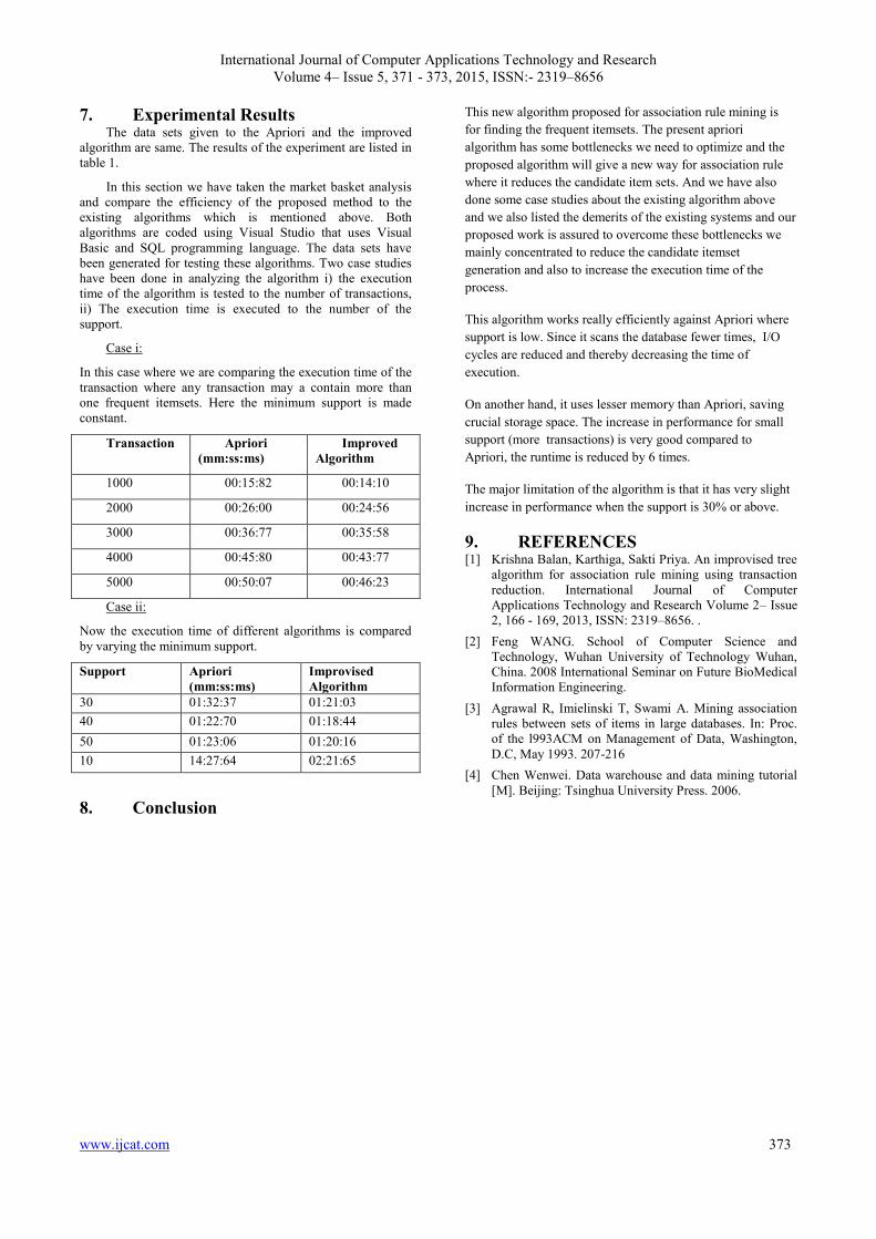
International Journal of Computer Applications Technology and Research
Volume 4– Issue 5, 371 - 373, 2015, ISSN:- 2319–8656
www.ijcat.com 373
7. Experimental Results The data sets given to the Apriori and the improved
algorithm are same. The results of the experiment are listed in
table 1.
In this section we have taken the market basket analysis
and compare the efficiency of the proposed method to the
existing algorithms which is mentioned above. Both
algorithms are coded using Visual Studio that uses Visual
Basic and SQL programming language. The data sets have
been generated for testing these algorithms. Two case studies
have been done in analyzing the algorithm i) the execution
time of the algorithm is tested to the number of transactions,
ii) The execution time is executed to the number of the
support.
Case i:
In this case where we are comparing the execution time of the
transaction where any transaction may a contain more than
one frequent itemsets. Here the minimum support is made
constant.
Transaction Apriori
(mm:ss:ms)
Improved
Algorithm
1000 00:15:82 00:14:10
2000 00:26:00 00:24:56
3000 00:36:77 00:35:58
4000 00:45:80 00:43:77
5000 00:50:07 00:46:23
Case ii:
Now the execution time of different algorithms is compared
by varying the minimum support.
Support Apriori
(mm:ss:ms)
Improvised
Algorithm
30 01:32:37 01:21:03
40 01:22:70 01:18:44
50 01:23:06 01:20:16
10 14:27:64 02:21:65
8. Conclusion
This new algorithm proposed for association rule mining is
for finding the frequent itemsets. The present apriori
algorithm has some bottlenecks we need to optimize and the
proposed algorithm will give a new way for association rule
where it reduces the candidate item sets. And we have also
done some case studies about the existing algorithm above
and we also listed the demerits of the existing systems and our
proposed work is assured to overcome these bottlenecks we
mainly concentrated to reduce the candidate itemset
generation and also to increase the execution time of the
process.
This algorithm works really efficiently against Apriori where
support is low. Since it scans the database fewer times, I/O
cycles are reduced and thereby decreasing the time of
execution.
On another hand, it uses lesser memory than Apriori, saving
crucial storage space. The increase in performance for small
support (more transactions) is very good compared to
Apriori, the runtime is reduced by 6 times.
The major limitation of the algorithm is that it has very slight
increase in performance when the support is 30% or above.
9. REFERENCES [1] Krishna Balan, Karthiga, Sakti Priya. An improvised tree
algorithm for association rule mining using transaction
reduction. International Journal of Computer
Applications Technology and Research Volume 2– Issue
2, 166 - 169, 2013, ISSN: 2319–8656. .
[2] Feng WANG. School of Computer Science and
Technology, Wuhan University of Technology Wuhan,
China. 2008 International Seminar on Future BioMedical
Information Engineering.
[3] Agrawal R, Imielinski T, Swami A. Mining association
rules between sets of items in large databases. In: Proc.
of the l993ACM on Management of Data, Washington,
D.C, May 1993. 207-216
[4] Chen Wenwei. Data warehouse and data mining tutorial
[M]. Beijing: Tsinghua University Press. 2006.
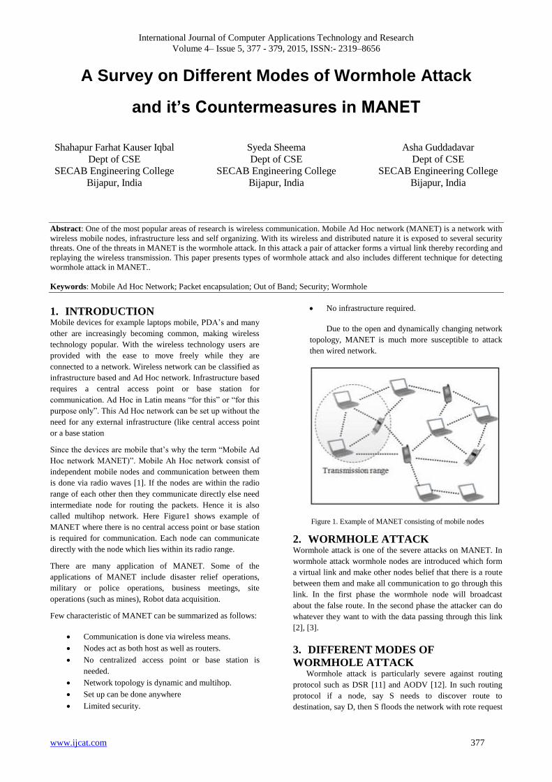
International Journal of Computer Applications Technology and Research
Volume 4– Issue 5, 377 - 379, 2015, ISSN:- 2319–8656
www.ijcat.com 377
A Survey on Different Modes of Wormhole Attack
and it’s Countermeasures in MANET
Shahapur Farhat Kauser Iqbal
Dept of CSE
SECAB Engineering College
Bijapur, India
Syeda Sheema
Dept of CSE
SECAB Engineering College
Bijapur, India
Asha Guddadavar
Dept of CSE
SECAB Engineering College
Bijapur, India
Abstract: One of the most popular areas of research is wireless communication. Mobile Ad Hoc network (MANET) is a network with
wireless mobile nodes, infrastructure less and self organizing. With its wireless and distributed nature it is exposed to several security
threats. One of the threats in MANET is the wormhole attack. In this attack a pair of attacker forms a virtual link thereby recording and
replaying the wireless transmission. This paper presents types of wormhole attack and also includes different technique for detecting
wormhole attack in MANET..
Keywords: Mobile Ad Hoc Network; Packet encapsulation; Out of Band; Security; Wormhole
1. INTRODUCTION Mobile devices for example laptops mobile, PDA’s and many
other are increasingly becoming common, making wireless
technology popular. With the wireless technology users are
provided with the ease to move freely while they are
connected to a network. Wireless network can be classified as
infrastructure based and Ad Hoc network. Infrastructure based
requires a central access point or base station for
communication. Ad Hoc in Latin means “for this” or “for this
purpose only”. This Ad Hoc network can be set up without the
need for any external infrastructure (like central access point
or a base station
Since the devices are mobile that’s why the term “Mobile Ad
Hoc network MANET)”. Mobile Ah Hoc network consist of
independent mobile nodes and communication between them
is done via radio waves [1]. If the nodes are within the radio
range of each other then they communicate directly else need
intermediate node for routing the packets. Hence it is also
called multihop network. Here Figure1 shows example of
MANET where there is no central access point or base station
is required for communication. Each node can communicate
directly with the node which lies within its radio range.
There are many application of MANET. Some of the
applications of MANET include disaster relief operations,
military or police operations, business meetings, site
operations (such as mines), Robot data acquisition.
Few characteristic of MANET can be summarized as follows:
Communication is done via wireless means.
Nodes act as both host as well as routers.
No centralized access point or base station is
needed.
Network topology is dynamic and multihop.
Set up can be done anywhere
Limited security.
No infrastructure required.
Due to the open and dynamically changing network
topology, MANET is much more susceptible to attack
then wired network.
Figure 1. Example of MANET consisting of mobile nodes
2. WORMHOLE ATTACK Wormhole attack is one of the severe attacks on MANET. In
wormhole attack wormhole nodes are introduced which form
a virtual link and make other nodes belief that there is a route
between them and make all communication to go through this
link. In the first phase the wormhole node will broadcast
about the false route. In the second phase the attacker can do
whatever they want to with the data passing through this link
[2], [3].
3. DIFFERENT MODES OF
WORMHOLE ATTACK Wormhole attack is particularly severe against routing
protocol such as DSR [11] and AODV [12]. In such routing
protocol if a node, say S needs to discover route to
destination, say D, then S floods the network with rote request

International Journal of Computer Applications Technology and Research
Volume 4– Issue 5, 377 - 379, 2015, ISSN:- 2319–8656
www.ijcat.com 378
message. The node that receives the request packet processes
the packet, adds its own identity and rebroadcast it. In order to
limit the amount of flooding each node only broadcast the first
packet it receives and drops further copies of same request.
When destination node D receives the request it generates a
route reply and sends back to S. The sender node then selects
the best route from all the route reply it has received. Best
route is selected on basis of shortest route. In case of
wormhole attack the node at one end hears the route request
and tunnels it to the wormhole node at the other end of tunnel.
The wormhole nodes give false illusion that the route passing
through them is the shortest, even though they are not.
Wormhole can be classified into four modes-packet
encapsulation, packet relay, high power transmission and out-
of-B-band [13].
3.1 Packet Encapsulation
In packet encapsulation the wormhole node on one end
encapsulates the packet to prevent nodes on the way from
incrementing node count. When the wormhole node at the
other end receives this packet it will bring the packet to its
original form. Figure 2 below shows an example of packet
encapsulation where node C and node J are wormhole
nodes.
Figure 2. Example of packet encapsulation in wormhole attack
3.2 Packet Relay
In this type of attack two malicious nodes relay the packets
between them which are far apar but make illution of being
neighbor.
3.3 High Power Transmission
In this kind of attack there exist only one malicious node
which has high transmission power used to attract packets to
pass through it.
3.4 Out Of Band
In Out-of-band wormhole attack the attacked node form an
external link between the two nodes to form a tunnel. The
wormhole node then advertises about the shortest path and
makes all the communication pass through it. This can be
further classified as High power transmission. In high power
transmission the attacked node has much higher capability
that lures other nodes to send packets to go through this path.
Figure 3. Out-Of-Band Wormhole Attack
Here figure 3 shows Out-Of-Band wormhole attack in which
node C and node J forms an external link or in other words a
tunnel through which all communication can be captured. The
wormhole node will advertise that there is a shortest path
between node C and node J and make all communication go
through this link.
4. DIFFERENT DETECTION METHODS Several researchers have worked on detection of wormhole
attack in MANET. Some of the detection methods discussed
in next section.
4.1 Hop Count Analysis Method Shang, Laih and Kau[4] introduced a method called hop count
analysis for detection of wormhole. This method does not
really identify the wormhole but simply avoids the route that
is suspected to have wormhole and selects a different route.
The author introduced a multipath routing protocol that is
based on hop count analysis method. The idea is to use split
multipath route and so the data is also split. With this the
attacker cannot completely seize the data.
4.2 Location Based Approach Location based approach is useful where the location of
neighboring nodes and transmission range are known. In this
technique the nodes share their location information with each
other. Author of [5] proposed a special method called the
geographical leash to detect wormhole. A leash is some
information which is attached to a packet designed to control
the maximum allowed transmission distance. This geographic
leash ensures that the receiver of the packet is within the
range of sender. Initially all nodes know their own location.
The node while sending a packet includes time when the
packet was sent, time when packet was received and its

International Journal of Computer Applications Technology and Research
Volume 4– Issue 5, 377 - 379, 2015, ISSN:- 2319–8656
www.ijcat.com 379
location. The recipient node now compares this information
with its own location and time when the packet was received.
In location based approach special hardware is used. Location
based is equipped with either GPS or some positioning
technology. This technology fails in the absence of GPS
system.
4.3 Time Based Approach Time pased approach proposed by Hu et al [5][6] is based on
accurate time measurement. This technique requires the nodes
to maintain tightly synchonized clock. The author has
proposed a technique called temporal leash. In this method
extremly accurate clock synchonization is needed to bound
propogation time of packet. In [7], the author has proposed a
methode called transmission time based mechanism(TTM).
Thia method detects wormhole during early stage of route set
up by calculating the time of transmission between two
successive nodes. If the transmission time betweenn two
nodes is high then wormhole is detected. It doesa not require
any special harware like GPS system.
4.4 Digital Signature Based Approach
In [8] author has proposed a method using digital signature.
All nodes in network contains digital signature of every other
nodes in the same network. A trusted path is created between
the sender and the receiver using digital signature. If a node
does not have legal digital signature, it is identified a
malicious node.
4.4 Neighbor Node Monitoring Author of [9] has proposed a method based on a response time
of reply message. This response time is used for
authentication purpose. All nodes maintain table for storing
the reply time. If the reply time is not accurate then there is a
malicious node in the network. Comparison is done on
response time and repeated until destination is reached.
4.5 Round Trip Time Based Approach The Round Trip Time (RTT) based approach proposed by
Zaw Tun and Thein [10] considers the round trip time (RTT)
between two successive nodes. Based on transmission time
between two nodes wormhole is detected. Here the
transmission time between two false nodes is considered to be
higher than others. This technique does not require any kind
of special hardware for its detection process.
5. CONCLUSION Due to the open nature and dynamic network topology of
MANET, it is much more vulnerable to attacks. This paper
discusses a particularly severe attack that is the wormhole
attack and its different types in detail. Wormhole attack has
different modes through which it can capture and disrupt the
packets. It can either hide the route information by packet
encapsulation or form a tunnel between the attacked nodes to
pass all packets through this tunnel. Various countermeasures
are also discussed here which are used to detect the wormhole
attack in MANET.
6. REFERENCES [1] C. Siva Ram Murthy and B.S.Manoj, “Ad hoc Wireless
Networks” (Chapter 7), 2014.
[2] Jyoti Thalor, Ms. Monika “Wormhole Attack Detection
and Prevention Technique in Mobile Ad Hoc Networks:
A Review”, International Journal of Advanced Research
in Computer Science and Software Engineering -
Volume 3, Issue 2, February 2013.
[3] Reshmi Maulik and Nanbendu Chaki: “A Study on
Wormhole Attacks in MANET” International Journal of
Computer Information System and Industrial
Management Applications (IJCISIM),Vol.3 (2011), pp.
271-279.
[4] Jen S.-M.; Laih C.-S.; Kuo W.-C. A Hop-Count Analysis
Scheme for Avoiding Wormhole Attacks in MANET.
Sensors. 2009.
[5] Yih-Chun Hu, Adrian Perig, David B. Johnson:
“Wormhole Attack on Wireless Network” IEEE
JOURNAL ON SELECTED AREAS IN
COMMUNICATIONS, Vol. 24- No 2, 2006.
[6] Y.C.Hu, A.Perrig and D.Johnson: “Packet leashes: a
defense against wormhole attacks in wireless networks,”
in INFOCOM, 2003.
[7] Phuong Van Tran, Le Xuan Hung, Young-Koo Lee,
Sungyoung Lee and Heejo Lee: “TTM: An Efficient
Mechanism to Detect Wormhole Attacks in Wireless Ad-
hoc Networks” IEEE CCNC, 2007.
[8] Pallavi Sharma, Prof. Aditya Trivedi, "An Approach to
Defend Against Wormhole Attack in Ad Hoc Network
Using Digital Signature”, IEEE, 2011.
[9] sweety goyai, harish rohil, “Securing MANET against
Wormhole Attacl using Neighbour Node Analysis” IJCA
volume 81,November 2013.
[10] Zaw Tun and Ni Lar Thein “Round Trip Time Based
Wormhole Attack Detection” ICCA 2009
[11] D. Johnson, D. Maltz, and J. Broch, The Dynamic
Source Routing Protocol for Multihop Wireless Ad Hoc
Networks, in Ad Hoc Networking, Addison-Wesley,
2001.
[12] C. E. Perkins and E. M. Royer, Ad-Hoc On-Demand
Distance Vector Routing, in Proceedings of the Second
IEEE Workshop on Mobile Computing Systems and
Applications (WMCSA’99), pp. 90-100, February 1990.
[13] Himanshu Prajapati “Techniques for Detection &
Avoidance of Wormhole Attack in Wireless Ad Hoc
Networks” Vol. 3 Issue 3, March-2014, pp: (21-27)

International Journal of Computer Applications Technology and Research
Volume 4– Issue 5, 380 - 385, 2015, ISSN:- 2319–8656
www.ijcat.com 380
A Survey on Selective Jamming Attacks in WMNs
Syeda Arshiya Sultana Samreen Banu kazi Parveen Maniyar M. Azharuddin
Dept of CSE, Dept of CSE, Dept of CSE, Dept of CSE
S.I.E.T, Vijayapur, S.I.E.T, Vijayapur, S.I.E.T, Vijayapur, S.I.E.T, Vijayapur
Karnataka, India Karnataka, India Karnataka, India Karnataka, India
Abstract—Wireless mesh networks (WMNs) assure to expand high-speed wireless connectivity beyond what is possible
with the current Wi-Fi based infrastructure. Due to their unique architectural features leave them particularly vulnerable to
security threats. In this paper, various forms of sophisticated attacks launched from adversaries with internal access to the
WMN are described. We also identify possible detection and mitigation mechanisms.
Keywords—Security, wireless mesh networks, jamming, misbehaviour, insider attacks, packet drop
1. INTRODUCTION
Wireless mesh networks (WMNs) are continuously
receiving significant interest as a possible means of
providing seamless data connectivity, especially in urban
environments [1]. Such networks evolved from classic
mobile ad hoc networks, targeting long-range
transmissions with importance on network throughput
and connectivity. WMN applications include stationary
deployments e.g., community networks, hierarchal sensor
networks as well as mobile ones e.g., intelligent
transportation systems, tactical military networks.
WMNs follow two-tier network architecture [2].
The first tier consists of the end users, also referred to
as stations (STAs), and directly connected to mesh nodes
referred to as Mesh Access Points (MAPs). The second
tier consists of a peer-to-peer network of the MAPs.
Connectivity in the second tier is assisted by intermediate
routers known as Mesh Points (MPs) which interconnect
MAPs (MPs do not accept connections from end users).
The network of MAPs and MPs is often static and uses
separate frequency bands to communicate data and
control information (MAPs are typically equipped with
multiple transceivers). Finally, Mesh Gateways (MGs)
provide connectivity to the wired infrastructure. An
example of a WMN is shown in Fig. 1.
WMNs are always vulnerable to “external” and
“internal” attacks. External attacks take the forms of
random channel jamming, packet replay, and packet
fabrication, and are launched by “foreign” devices that
are unaware of the network secrets e.g., cryptographic
credentials and pseudo-random spreading codes. They
are relatively easier to counter through a combination of
Cryptography based and robust communication
techniques. Internal attacks, which are launched from
compromised nodes, are much more difficult in nature.
These attacks use knowledge of network secrets and
protocol semantics to selectively and adaptively target
critical network functions. By overhearing the first few
bits of a packet, or classification transmissions based on
protocol semantics, attack selectivity can be achieved.
Internal attacks, hereafter referred to as insider attacks,
cannot be mitigated using only proactive methods which
rely on network secrets, because the attacker already has
access to such secrets.
Fig.1 Architecture of WMN
They additionally require protocols with built-in security
measures, through which the attacker can be detected and
its selective nature can be neutralized.
1.1 Vulnerabilities of WMNs: While all types of wireless
networks are vulnerable to insider attacks, for a number
of reasons WMNs are mainly susceptible. First, MPs and
MAPs are relatively cheap devices with poor physical
security, which makes them potential targets for node
capture and compromise. Second, given their relatively
advanced hardware e.g., multiple transceivers per MP
and MAP, WMNs frequently adopt a multi-channel
design, with one or more channels dedicated for control
or broadcast purposes. Such static design makes it easier
for an attacker to selectively target control or broadcast
information. Third, the reliance on multihop routes
further accentuates the WMN vulnerability to
compromised relays which can drop control messages, in
order to enforce a certain routing behaviour e.g., force
packets to follow long or inconsistent routes.
2. SELECTIVE JAMMING ATTACKS
The open nature of the wireless medium makes
it susceptible to jamming attacks. Jamming is a severe
form of DoS (Denial of Service) attack. In wireless
networks jamming has been primarily analyzed under an
external adversarial model. Existing anti-jamming
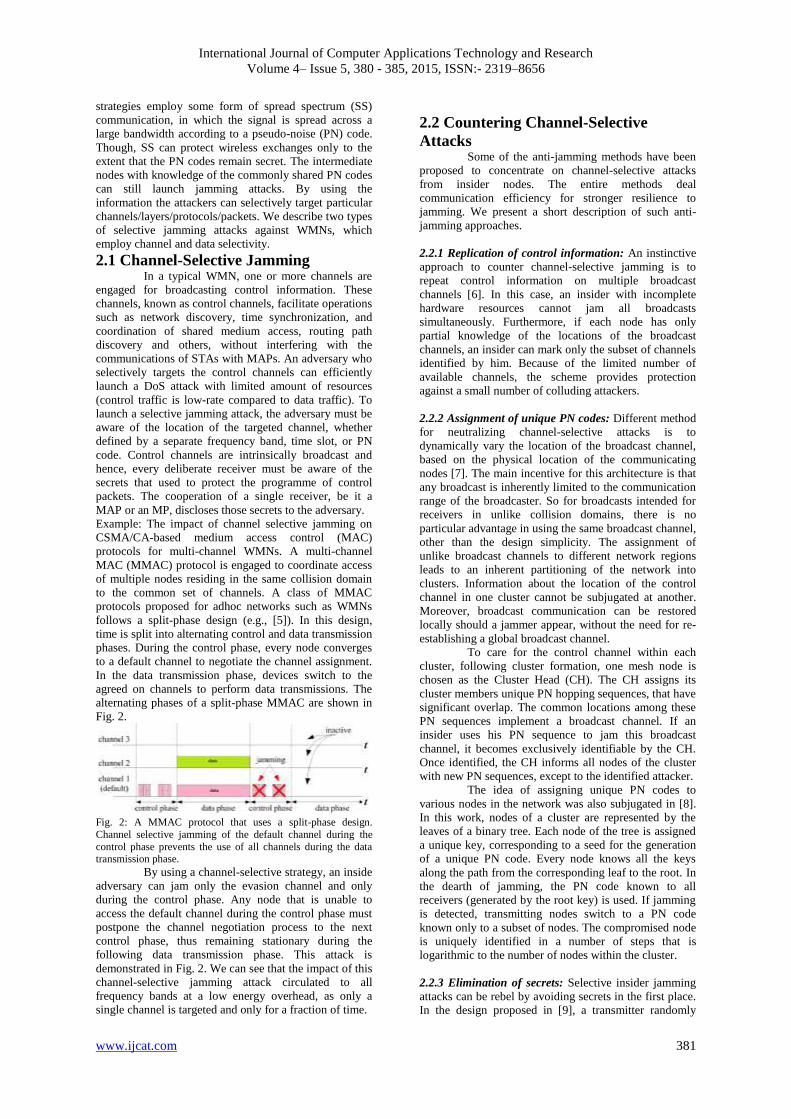
International Journal of Computer Applications Technology and Research
Volume 4– Issue 5, 380 - 385, 2015, ISSN:- 2319–8656
www.ijcat.com 381
strategies employ some form of spread spectrum (SS)
communication, in which the signal is spread across a
large bandwidth according to a pseudo-noise (PN) code.
Though, SS can protect wireless exchanges only to the
extent that the PN codes remain secret. The intermediate
nodes with knowledge of the commonly shared PN codes
can still launch jamming attacks. By using the
information the attackers can selectively target particular
channels/layers/protocols/packets. We describe two types
of selective jamming attacks against WMNs, which
employ channel and data selectivity.
2.1 Channel-Selective Jamming In a typical WMN, one or more channels are
engaged for broadcasting control information. These
channels, known as control channels, facilitate operations
such as network discovery, time synchronization, and
coordination of shared medium access, routing path
discovery and others, without interfering with the
communications of STAs with MAPs. An adversary who
selectively targets the control channels can efficiently
launch a DoS attack with limited amount of resources
(control traffic is low-rate compared to data traffic). To
launch a selective jamming attack, the adversary must be
aware of the location of the targeted channel, whether
defined by a separate frequency band, time slot, or PN
code. Control channels are intrinsically broadcast and
hence, every deliberate receiver must be aware of the
secrets that used to protect the programme of control
packets. The cooperation of a single receiver, be it a
MAP or an MP, discloses those secrets to the adversary.
Example: The impact of channel selective jamming on
CSMA/CA-based medium access control (MAC)
protocols for multi-channel WMNs. A multi-channel
MAC (MMAC) protocol is engaged to coordinate access
of multiple nodes residing in the same collision domain
to the common set of channels. A class of MMAC
protocols proposed for adhoc networks such as WMNs
follows a split-phase design (e.g., [5]). In this design,
time is split into alternating control and data transmission
phases. During the control phase, every node converges
to a default channel to negotiate the channel assignment.
In the data transmission phase, devices switch to the
agreed on channels to perform data transmissions. The
alternating phases of a split-phase MMAC are shown in
Fig. 2.
Fig. 2: A MMAC protocol that uses a split-phase design.
Channel selective jamming of the default channel during the
control phase prevents the use of all channels during the data transmission phase.
By using a channel-selective strategy, an inside
adversary can jam only the evasion channel and only
during the control phase. Any node that is unable to
access the default channel during the control phase must
postpone the channel negotiation process to the next
control phase, thus remaining stationary during the
following data transmission phase. This attack is
demonstrated in Fig. 2. We can see that the impact of this
channel-selective jamming attack circulated to all
frequency bands at a low energy overhead, as only a
single channel is targeted and only for a fraction of time.
2.2 Countering Channel-Selective
Attacks Some of the anti-jamming methods have been
proposed to concentrate on channel-selective attacks
from insider nodes. The entire methods deal
communication efficiency for stronger resilience to
jamming. We present a short description of such anti-
jamming approaches.
2.2.1 Replication of control information: An instinctive
approach to counter channel-selective jamming is to
repeat control information on multiple broadcast
channels [6]. In this case, an insider with incomplete
hardware resources cannot jam all broadcasts
simultaneously. Furthermore, if each node has only
partial knowledge of the locations of the broadcast
channels, an insider can mark only the subset of channels
identified by him. Because of the limited number of
available channels, the scheme provides protection
against a small number of colluding attackers.
2.2.2 Assignment of unique PN codes: Different method
for neutralizing channel-selective attacks is to
dynamically vary the location of the broadcast channel,
based on the physical location of the communicating
nodes [7]. The main incentive for this architecture is that
any broadcast is inherently limited to the communication
range of the broadcaster. So for broadcasts intended for
receivers in unlike collision domains, there is no
particular advantage in using the same broadcast channel,
other than the design simplicity. The assignment of
unlike broadcast channels to different network regions
leads to an inherent partitioning of the network into
clusters. Information about the location of the control
channel in one cluster cannot be subjugated at another.
Moreover, broadcast communication can be restored
locally should a jammer appear, without the need for re-
establishing a global broadcast channel.
To care for the control channel within each
cluster, following cluster formation, one mesh node is
chosen as the Cluster Head (CH). The CH assigns its
cluster members unique PN hopping sequences, that have
significant overlap. The common locations among these
PN sequences implement a broadcast channel. If an
insider uses his PN sequence to jam this broadcast
channel, it becomes exclusively identifiable by the CH.
Once identified, the CH informs all nodes of the cluster
with new PN sequences, except to the identified attacker.
The idea of assigning unique PN codes to
various nodes in the network was also subjugated in [8].
In this work, nodes of a cluster are represented by the
leaves of a binary tree. Each node of the tree is assigned
a unique key, corresponding to a seed for the generation
of a unique PN code. Every node knows all the keys
along the path from the corresponding leaf to the root. In
the dearth of jamming, the PN code known to all
receivers (generated by the root key) is used. If jamming
is detected, transmitting nodes switch to a PN code
known only to a subset of nodes. The compromised node
is uniquely identified in a number of steps that is
logarithmic to the number of nodes within the cluster.
2.2.3 Elimination of secrets: Selective insider jamming
attacks can be rebel by avoiding secrets in the first place.
In the design proposed in [9], a transmitter randomly

International Journal of Computer Applications Technology and Research
Volume 4– Issue 5, 380 - 385, 2015, ISSN:- 2319–8656
www.ijcat.com 382
selects a PN code from a public codebook. To recover a
transmitted packet, receivers must record the transmitted
signal and attempt decoding it using every PN code in
the codebook. Because the PN code used to spread each
packet is not known a priori, an inside adversary can only
attempt to guess it, with a limited probability of success.
Special care needs to be given to the management
between the communicating parties (knowing the PN
code is essential for discovering and “Locking onto” the
transmitted signal).
2.3 Data-Selective Jamming Further to progress the energy efficiency of selective
jamming and reduce the risk of detection, an inside
attacker can use a greater degree of selectivity by
targeting specific packets of high importance. One way
of launching a data-selective jamming attack, is by
classifying packets before their transmission is
completed. An example of this
Fig. 3(a) A data-selective jamming attack
Fig. 3(b) generic packet format
attack is shown in Fig. 3(a). MPA transmits a packet to
MPB. Inside attacker MAPJ classifies the transmitted
packet after overhearing its first few bytes. MAPJ then
interferes with the reception of the rest of the packet at
MPB. Referring to the generic packet format in Fig. 3(b),
a packet can be classified based on the headers of various
layers.
Fig. 3(c) inference of a RREP transmission on link MAPB-
STAC
For example, the MAC header typically contains
information about the next hop and the packet type. The
TCP header reveals the end-to-end source and destination
nodes, the transport-layer packet type (SYN, ACK,
DATA, etc.), and other TCP parameters. Another method
for packet classification is to anticipate a transmission
based on protocol semantics. As an example, consider the
routing function in WNMs, described in the IEEE
802.11s standard [2]. Routing is performed at the MAC
layer according to the Hybrid Wireless Mesh Protocol
(HWMP). The latter is a combination of tree-based
routing, and on-demand routing based on AODV. Tree-
based routing provides fixed path routes from the mesh
nodes to the MGs. On demand routing is employed to
discover routes to mobile STAs who associate with
multiple MAPs due to their mobility. Consider the route
discovery process depicted in Fig. 3(c). MPA transmits a
route reply (RREP) to MAPB, which is listening in by
MAPJ. MAPJ can conjecture that MAPB will forward the
RREP to STAC, and hence, jam this RREP while it is in
transit to STAC.
Packet classification can also be achieved by
observing implicit packet identifiers such as packet
length, or precise protocol timing information [4]. For
example, control packets are usually much smaller than
data packets. The packet length of an eminent
transmission can be inferred by decoding the network
allocation vector field (NAV) of request-to-send (RTS)
and clear-to-send (CTS) messages, used for reserving the
wireless medium.
2.4 Countering Data-Selective Jamming
Attacks An instinctive solution for preventing packet
classification is to encrypt transmitted packets with a
secret key. In this case, the entire packets, including its
headers, have to be encrypted. While a shared key be
sufficient to protect point-to-point-communications, for
broadcast packets, this key must be shared by all
intended receivers. Therefore, this key is also known to
an inside jammer. In symmetric encryption schemes
based on block encryption, reception of one cipher text
block is sufficient to obtain the corresponding plaintext
block, if the decryption key is known. Thus, encryption
alone does not prevent insiders from classifying
broadcasted packets.
To avert classification, a packet must remain
hidden until it is transmitted in its entirety. One possible
way for temporarily hiding the transmitted packet is to
employ commitment schemes. In a commitment scheme,
the transmitting node hides the packet by broadcasting a
committed version of it. The contents of the packet
cannot be inferred by receiving the commitment (hiding
property). After the transmission is completed, the node
releases a de-commitment value, which reveals the
original packet. The commitment scheme must be
carefully designed to prevent the classification of the
original packet based on the partial release of the de-
commitment value. Another approach is to use public
hiding transformations that do not rely on secrets. An
example of them is all-or-nothing transformations
(AONTs), which were originally proposed to slow down
brute force search attacks against encryption schemes.
An AONT serves as a publicly known and completely
invertible pre-processing step for a plaintext, before it is
passed to an encryption algorithm. The defining property
of an AONT is that the entire output of the
transformation must be known before any part of the
input can be computed. In our context, an AONT
prevents packet classification when the AONT of a
packet is transmitted over the wireless medium.

International Journal of Computer Applications Technology and Research
Volume 4– Issue 5, 380 - 385, 2015, ISSN:- 2319–8656
www.ijcat.com 383
3. SELECTIVE DROPPING
ATTACKS If selective jamming is not successful due to
anti-jamming measures, an insider can selectively drop
packets post-reception. Once a packet has been received,
the cooperated node can inspect that the packet headers,
classify the packet, and decide whether to forward it or
not. Such an action is often termed as misbehaviour [10]–
[13]. Post-reception dropping is less flexible than
selective jamming because the adversary is restricted to
dropping only the packets routed through it. Nonetheless,
the impact on the WMN performance can be significant.
Examples: Consider a compromised MP targeting the
routing functionality in WMNs. By selectively dropping
route request and route reply packets employed by the
routing protocol, as defined in the of the 802.11s
standard [2], the compromised MP can prevent the
discovery of any route that passes through it, delay the
route discovery process, and force alternative, possibly
inefficient paths.
Alternatively, the compromised MP can allow
the establishment of a route via itself, but throttle the rate
of the end-to-end connection at the transport layer. This
attack can be actualized by selective dropping of critical
control packets that regulate the end-to-end transmission
rate and effective throughput. For example, the dropping
of cumulative TCP acknowledgments results in the end-
to- end retransmission of the entire batch of pending data
packets (see Fig. 4). In addition, packet loss is interpreted
as congestion, resulting in the throttling of the sender’s
transmission rate. In another selective strategy known as
the Jellyfish attack, a compromised mesh node that
periodically drops a small fraction of consecutive packets
can effectively reduce the throughput of a TCP flow to
near zero [14]. This attack can be achieved even by
inducing random delays to TCP packets, without
dropping them, while remaining protocol compliant [14].
Similar selective dropping attacks can be constructed for
other network functions such as the association/de-
association of STAs, and topology management, to name
a few.
Fig. 4. An insider selectively drops cumulative TCP
acknowledgments and forces end-to-end data retransmissions.
3.1 Mitigation of Selective Dropping Selective dropping attacks can be mitigated by
employing fault-tolerant mechanisms at various layers of
the protocol stack. At the routing layer, multi-path
routing provides robust multi-hop communication in the
presence of network faults, by utilizing more than one
path from a source to a destination. Tree-based routing in
HWMP already provisions for back-up paths to the MG
[2]. At the transport layer, variants of the standardized
TCP protocol have been specifically developed for
dealing with the imperfections of the wireless medium
[15]. These protocols differentiate between congestion
and wireless transmission losses. A selective dropper can
always attribute his losses to congestion, in order to
avoid detection as a malicious node. In this case,
identification mechanisms employing long-term
statistics, can accurately pinpoint selective droppers.
3.1.1 Identification of Selective Droppers
Current methods for detecting misbehaviour in self
organizing systems such as WMNs, can be classified into
reputation systems [12], credit-based systems [13], and
acknowledgment systems [10].
Reputation Systems: Reputation systems identify
misbehaving nodes based on per-node reputation metrics,
computed based on interactions of each node with its
peers. These systems typically incorporate two critical
operations: (a) the collection of accurate observations of
nodes’ behaviour and, (b) the computation of the
reputation metric. Behavioral information is collected
based on first-hand observations provided by
neighboring nodes and second hand information
provided by other interacting peers [12]. First-hand
observations are collected by monitoring nodes which
operate in promiscuous mode in order to confirm the
correct forwarding of transmitted packets. Overhearing
becomes problematic in the case of multichannel WMNs,
because MPs and MAPs are scheduled to communicate
in parallel over orthogonal frequency bands, and hence,
they might not be available to monitor the behavior of
other nodes. Several schemes have been proposed for
managing second-hand information. A node may flood
warnings to the entire network, if it detects a
misbehaving node. Then again, information can be
provided on-demand, after a request from a particular
node has been received. In the latter scenario, flooding of
the request is necessary to discover nodes that possess
second-hand information. Both methods consume
considerable bandwidth resources due to the underlying
flooding operations for the dissemination and collection
of second-hand information. Robust computation of
reputation metrics is equally important for the
identification of packet droppers. Simple aggregate
metrics have been shown to be vulnerable to false
accusations from colluding malicious nodes, and
suddenly changing behavioral patterns. For instance, a
misbehaving node can exhibit a long history of good
behavior in order to build a high reputation metric, before
it starts to misbehave. Such instances are dealt by
assigning larger weights to recent behavioral
observations and/or adopting additive increase-
multiplicative decrease type of algorithms for updating
the reputation metrics [12].
A critical challenge for any metric computation
algorithm is the selective nature of packet droppers.
When a very small fraction of packets is dropped, metrics
that do not take into account the packet type are bound to
have high rates of misdetection. Dropping selectivity can
be detected with the use of storage-efficient reports (e.g.,
based on Bloom filters) of the per-packet behavior
of nodes [11]. Based on these reports, it is possible to
conduct multiple tests to identify malicious selective
dropping patterns. These patterns are likely to have some
deterministic structure compared to packet losses due to
congestion or poor channel quality. ACK-based systems:
ACK-based schemes differ from overhearing techniques
in the method of collecting first-hand behavioral
observations. Downstream nodes (more than a single hop

International Journal of Computer Applications Technology and Research
Volume 4– Issue 5, 380 - 385, 2015, ISSN:- 2319–8656
www.ijcat.com 384
away) are responsible for acknowledging the reception of
messages to nodes several hops upstream [10]. These
systems are suitable for monitoring the faithful relay of
unicast traffic, at the expense of communication
overhead for relaying an additional set of ACKs.
However, ACK-based schemes cannot be used to identify
insiders that selectively drop broadcast packets. Such
packets remain, in general, unacknowledged in wireless
networks, to avoid an ACK implosion situation.
Moreover, a small set of colluding nodes can still provide
authentic ACKs to upstream nodes while dropping
packets.
Credit-based systems: Credit-based systems lessen
selfish behavior by incentivising nodes to forward
packets [13]. Nodes that relay traffic receive credit
in return, which can be later spent to forward their own
traffic. However, in the context of WNMs, MPs do not
generate any traffic of their own, but act as dedicated
relays. Hence, compromised MPs have no incentive for
collecting credit. Moreover, in the case of selective
dropping attacks, misbehaving nodes can still collect
sufficient credit by forwarding packets of low
importance, while dropping a few packets of “high
value.” In addition, the credit collected by a particular
node depends on the topology of the network. A highly
connected node is expected to collect more credit due to
the increased volumes of traffic routed through it. An
adversary cooperating such a node is likely able to
implement a selective dropping strategy without running
out of credit. Finally, credit-based systems lack a
mechanism for identifying the misbehaving node(s),
allowing them to remain within the network indefinitely.
4. DISCUSSION AND CONCLUSIONS
WMNs are exposed to various external and
internal security threats. While most external attacks can
be alleviated with a combination of cryptographic
mechanisms and robust communication techniques,
internal attacks are much harder to counter because the
adversary is aware of the network secrets and its
protocols. Jamming resistant broadcast communications
in the presence of inside jammers leftovers a challenging
problem. Present solutions attempt to eliminate the use of
common secrets for protecting broadcast
communications. Such secrets can be easily exposed in
the event of node compromise. Nevertheless, the
heightened level of security comes at the expense of
performance, because broadcasted messages have to be
transmitted multiple times and on multiple frequency
bands to guarantee robust reception.
Furthermore, even if packet reception of
critical messages is ensured, inside adversaries are in
complete control of the traffic routed through them. A
large body of literature addresses the problem of
misbehavior in the form of packet dropping by
developing reputation systems, credit-based systems, and
communication-intensive acknowledgment schemes.
Despite the relative wealth of literature on this problem,
significant challenges are yet to be addressed. Most
existing methods assume a continuously active adversary
that systematically drops packets. These adversaries are
detected by aggregate behavioral metrics such as per-
packet reputation and credit.
However, these metrics cannot detect attacks of
selective nature, where only a small fraction of “high
value” packets is targeted. Furthermore, when the
adversary drops only a few packet, his behavior can be
indistinguishable from dropping patterns due to
congestion or poor wireless conditions. Further
challenges include efficient behavioral monitoring
mechanisms not relying on continuous overhearing and
efficient maintenance and dissemination of reputation
metrics.
5. ACKNOWLEDGEMENT
Firstly we thanks to Almighty for his mercy on
us. We sincerely thank our Principal Dr. Syed Zakir Ali
for his support and guidance. We thank to Prof. Aslam
Karjagi for his support and we also thanks to Prof.
Mohammed Azharuddin for his guidance and continuous
encouragement. We thank our parents for their moral
support and also thanks to others who have supported us.
6. REFERENCES
[1] I.F.Akyildiz, X. Wang, and W. Wang. Wireless mesh
networks:a survey. Computer Networks, 47(4):445–487,
2005.
[2] IEEE P802.11s/D1.01 standard. At
https://mentor.ieee.org/802.11/dcn/07/11-07-0335-00-
000s-tgs-redline-between-draft-d1-00-and-d1-01.pdf,
2007.
[3] Alejandro, Proano and Loukas Lazos. Selective
jamming attacks in wireless networks. In proceedings of
the IEEE International Conference on Communications
(ICC), 2010.
[4] T.X.Brown, J.E. James, and A. Sethi. Jamming and
sensing of encrypted wireless ad hoc networks. In
Proceedings of the 7th ACM International Symposium on
Mobile ad hoc networking and computing, 2006.
[5] J. So and N.H. Vaidya. Multi-channel MAC for ad
hoc networks: handling multi-channel hidden terminals
using a single transceiver. In Proceedings of the ACM
MobiHoc Conference, pages 222–233, 2004.
[6] P.Tague, M. Li, and R. Poovendran. Probabilistic
mitigation of control channel jamming via random key
distribution. In Proceedings of the International
Symposium in Personal, Indoor and Mobile Radio
Communications (PIMRC), pages 1–5, 2007.
[7] L. Lazos, S. Liu, and M. Krunz. Mitigating control-
channel jamming attacks in multi-channel ad hoc
networks. In Proceedings of the Second ACM
Conference on Wireless Network Security (WiSec),
pages 169–180, 2009.
[8] Jerry Chiang and Yih-Chun Hu. Cross-layer jamming
detection and mitigation in wireless broadcast networks.
In Proceedings of the ACM MobiCom Conference, pages
346–349, 2007.
[9] Christina P´opper, Mario Strasser, and Srdjan
Capkun. Jamming resistant broadcast communication
without shared keys. In Proceedings of the USENIX
Security Symposium, 2009.
[10] K. Liu, J. Deng, P.K. Varshney, and K.
Balakrishnan. An acknowledgment-based approach for
the detection of routing misbehavior in MANETs. IEEE
Transactions on Mobile Computing,6(5):536–550, 2007.
[11] W. Kozma and L. Lazos. Dealing with liars:
Misbehavior identification via R´enyi-Ulam games. In
Security and Privacy in Communication Networks, pages
207–227, 2009.
[12] Han Yu, Zhiqi Shen, Chunyan Miao, C. Leung, and
D. Niyato. A survey of trust and reputation management
systems in wireless

International Journal of Computer Applications Technology and Research
Volume 4– Issue 5, 380 - 385, 2015, ISSN:- 2319–8656
www.ijcat.com 385
communications. Proceedings of the IEEE, 98(10):1755–
1772, 2010.
[13] Y. Zhang, W. Lou, W. Liu, and Y. Fang. A secure
incentive protocol for mobile ad hoc networks. Wireless
Networks, 13(5):569–582, 2007.
[14] Imad Aad, Jean-Pierre Hubaux, and Edward W.
Knightly. Impact of denial of service attacks on ad hoc
networks. IEEE/ACM Transactions on Networking,
16(4):791–802, 2008.
[15] J. Liu and S. Singh. ATCP: TCP for mobile ad hoc
networks.IEEE Journal on Selected Areas in
Communications,19(7):1300–1315, 2002.

International Journal of Computer Applications Technology and Research
Volume 4– Issue 5, 386 - 389, 2015, ISSN:- 2319–8656
www.ijcat.com 386
Hand Gesture Recognition using Colour Based
Segmentation and Hidden Markov Model
Kshitish Milind Deo
Computer Engineering
Department, Pune Institute of
Computer Technology, Pune,
India.
Avanti Yashwant Kulkarni
Computer Engineering
Department, Pune Institute of
Computer Technology, Pune,
India.
Tirtha Suresh Girolkar
Computer Engineering
Department, Pune Institute of
Computer Technology, Pune,
India.
Abstract: Automatic gesture recognition is a key technology used in Human Computer Interaction. In this paper we introduce a hand gesture
recognition system which consists of 4 modules, image segmentation, feature extraction, HMM training and gesture recognition. Image or
video is divided into multiple frames and segmentation process which uses colour based detection of the path of the object is applied to each
frame. Feature extraction process mainly considers the orientation of the state tracked. This is done using HSV[hue-saturation value] image
and contour mapping of the image. The training part of the HMM model works on basis of LRB(Left-Right-Banded)topology and uses the
BW (Baum Welch) algorithm. We have used Viterbi algorithm for mapping the state to a symbol i.e. recognition. HMM is used to predict
the gesture and increase the tolerance of the system to incorporate human errors.
Keywords: Hidden Markov Model (HMM), Forward Backward Algorithm, Baum Welch Algorithm, Viterbi Algorithm, Colour
Segmentation.
1. INTRODUCTION The goal of gesture interpretation is to enhance the advanced
human machine communication so as to make it more close to
human-human interaction. Few of the models used for this purpose
are Neural Networks, Fuzzy logic and HMMs. We are going to
propose a system which is based on HMM model.
In this paper, HMM model is used for dynamic hand gesture
recognition. HMMs can be successfully used for both speech and
two-dimensional signs, because their state based nature enables
them to capture variations in duration of signs, by remaining in
same state for several time frames. Gesture recognition is a step by
step process which has input as sequence of image frames and
output as a symbol.
Here, a system is developed to recognize geometric shapes drawn
with a blue coloured object. Colour is detected and pattern of hand
movement is analyzed. This gesture is divided into multiple states.
Output symbols are extracted from the gesture. These form
parameters for the Hidden Markov Model (HMM).Colour detection
technique has been used in our proposed system so as to track the
path of the object using which the desired shape is being drawn.
After the detection part the main issue is how to make the computer
understand the gesture. Recent works can be said to use two
methods: Data-glove based methods and vision based methods. The
Data Glove method uses sensor devices for digitizing hand and
finger motions for multi-parametric data. For Vision-based method,
the only required equipment is a camera.
Challenges in vision based system are, it needs to be background
invariant and lighting insensitive.
In the upcoming sections we will see how the segmentation part is
being done using colour filtering. We will briefly talk about the
process of feature extraction which requires contour detection and
calculation of centroid of each contour in each frame. Section 3.3
will be encompassing the explanation of how HMM training and
recognition works for our system.
2. HISTORY AND LITERATURE SURVEY
There exist many reported research projects related to learning and
recognizing visual behaviour. However due to its recent
introduction to the vision community, only a small number have
been reported which use Hidden Markov Models. HMM has been
traditionally used as tool for speech recognition tool, recent
researches have begun relating the speech variations to visual
gestures. Moni M. A. et al in their review paper [6] have analysed
various techniques and approaches in gesture recognition for sign
language recognition using HMM. They have provided an
overview of HMM and its use in vision based applications, working
in two stages that of image capturing and processing using cameras,
and the second stage for identifying and learning models has
eliminated the need of previously used sensor embedded equipment
such as gloves for tracking of a gesture. T. E. Stanner have
employed HMM in 1995 in identifying the American Sign
language. On similar grounds authors Gaus Y. F. A. et al have
successfully recognized the Malaysian Sign Language[5], skin
segmentation procedure throughout frames and feature extraction
by centroids, hand distances and orientation has been used, gesture
paths define the hand trajectory. Kalaman filters have been used by
researchers to identify overlaping hand-head and hand-hand
regions. In [1] Elmezain M, Al-Hamadi A, MichaelisB,have
quantized features form spatio-temporal trajectories into
codewords. They have used a novel method of tracking the gesture
by using 3D depth map along with colour information, this helps at
separating the same colour at different surfaces in a complex
background. In order to separate continuous gestures a special zero
codeword is defined, using the start and end points of meaningful
gestures the viterbi algorithm is employed or recognition. In [2]
the authors have used the LRB topology along with forward
algorithm to achieve the best performance. With a recognition rate
of 95.87% arabic numbers have been identified. Shrivastav R[3]
use OpenCV image processing library to perform the isolation of
gesture frames, the entire process form per-processing to testing. In
coordination with this processing, Baum-Welch algorithm and
LRB topology with forward algorithm is applied for recognition.
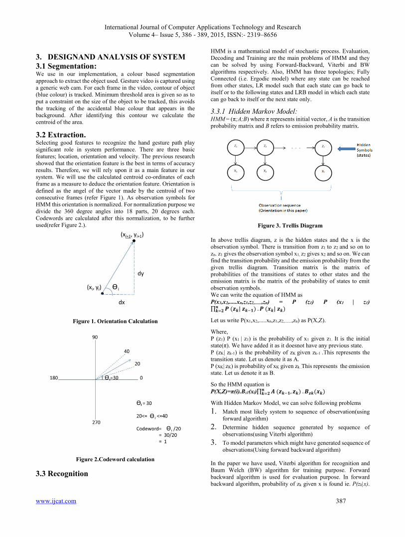
International Journal of Computer Applications Technology and Research
Volume 4– Issue 5, 386 - 389, 2015, ISSN:- 2319–8656
www.ijcat.com 387
3. DESIGNAND ANALYSIS OF SYSTEM
3.1 Segmentation: We use in our implementation, a colour based segmentation
approach to extract the object used. Gesture video is captured using
a generic web cam. For each frame in the video, contour of object
(blue colour) is tracked. Minimum threshold area is given so as to
put a constraint on the size of the object to be tracked, this avoids
the tracking of the accidental blue colour that appears in the
background. After identifying this contour we calculate the
centroid of the area.
3.2 Extraction. Selecting good features to recognize the hand gesture path play
significant role in system performance. There are three basic
features; location, orientation and velocity. The previous research
showed that the orientation feature is the best in terms of accuracy
results. Therefore, we will rely upon it as a main feature in our
system. We will use the calculated centroid co-ordinates of each
frame as a measure to deduce the orientation feature. Orientation is
defined as the angel of the vector made by the centroid of two
consecutive frames (refer Figure 1). As observation symbols for
HMM this orientation is normalized. For normalization purpose we
divide the 360 degree angles into 18 parts, 20 degrees each.
Codewords are calculated after this normalization, to be further
used(refer Figure 2.).
Figure 1. Orientation Calculation
Figure 2.Codeword calculation
3.3 Recognition
HMM is a mathematical model of stochastic process. Evaluation,
Decoding and Training are the main problems of HMM and they
can be solved by using Forward-Backward, Viterbi and BW
algorithms respectively. Also, HMM has three topologies; Fully
Connected (i.e. Ergodic model) where any state can be reached
from other states, LR model such that each state can go back to
itself or to the following states and LRB model in which each state
can go back to itself or the next state only.
3.3.1 Hidden Markov Model: HMM = (π;A;B) where π represents initial vector, A is the transition
probability matrix and B refers to emission probability matrix.
Figure 3. Trellis Diagram
In above trellis diagram, z is the hidden states and the x is the
observation symbol. There is transition from z1 to z2 and so on to
zn. z1 gives the observation symbol x1, z2 gives x2 and so on. We can
find the transition probability and the emission probability from the
given trellis diagram. Transition matrix is the matrix of
probabilities of the transitions of states to other states and the
emission matrix is the matrix of the probability of states to emit
observation symbols.
We can write the equation of HMM as
P(x1,x2,.....xn,z1,z2,.......,zn) = P (z1) P (x1 | z1) ∏ 𝑷 (𝒛𝒌| 𝒛𝒌−𝟏) . 𝑷 (𝒙𝒌| 𝒛𝒌) 𝒏
𝒌=𝟐
Let us write P(x1,x2,.....xn,z1,z2,.......,zn) as P(X,Z).
Where,
P (z1) P (x1 | z1) is the probability of x1 given z1. It is the initial
state(π). We have added it as it doesnot have any previous state.
P (zK| zk-1) is the probability of zK given zk-1 .This represents the
transition state. Let us denote it as A.
P (xK| zK) is probability of xK given zk .This represents the emission
state. Let us denote it as B.
So the HMM equation is
P(X,Z)=π(i).Bz1(xi)∏ 𝑨 (𝒛𝒌−𝟏, 𝒛𝒌) . 𝑩𝒛𝒌(𝒙𝒌) 𝒏𝒌=𝟐
With Hidden Markov Model, we can solve following problems
1. Match most likely system to sequence of observation(using
forward algorithm)
2. Determine hidden sequence generated by sequence of
observations(using Viterbi algorithm)
3. To model parameters which might have generated sequence of
observations(Using forward backward algorithm)
In the paper we have used, Viterbi algorithm for recognition and
Baum Welch (BW) algorithm for training purpose. Forward
backward algorithm is used for evaluation purpose. In forward
backward algorithm, probability of zk given x is found ie. P(zk|x).

International Journal of Computer Applications Technology and Research
Volume 4– Issue 5, 386 - 389, 2015, ISSN:- 2319–8656
www.ijcat.com 388
Assumption is that HMM parameters π(initial state), transition
probability and the emission probability is known. For this purpose
we use forward algorithm and backward algorithm.
In forward algorithm we calculate probability of zk given x1:k ie.
P(zk|x1:k). Note that when we write x1:k it means x1,x2……,xk.
In backward algorithm we calculate probability of xk+1:n given xk ie
P(xk+1:n|xk).
Thus the forward backward algorithm is the multiplication of the
two probabilities generated from the forward algorithm and
backward algorithm.
P(zk,x)=P(xk+1:n|zk,x1:k).P(zk,x1:k) In Viterbi algorithm, we find the maximum likelihood of the given
sequence to the trained model. Thus the goal is to find
Z*=argmaxP(z|x) .
4. EXPERIMENTATION ANALYSIS
4.1 Segmentation Our experiment consists of detecting the motion of blue coloured
object. Now one issue is that different shades of blue from the
background can get detected and create disturbance. To avoid this
we have specified a particular range of blue intensity that is to be
considered for detection. Range values used in our code are
min[95,50,70,0] and max[145,255,255,0].
Another issue which we deal with is the size of blue object. To
avoid detection of unnecessary blue objects we have put a
constraint of area of the object to be detected i.e. the area should be
greater than 1000{units}. Each frame is then passed to a filter
where contours of the object are drawn.
Figure 4. Image Segmentation
4.2 Feature Extraction Here, we used the Orientation feature for extraction. We first
calculated centroids of contour of each frame. Thus we got the
position of the blue spot in each frame. Using position of blue spot
in consecutive frames we calculated angle of orientation.
For convenience we have normalised the angle by forming groups
of 20 degrees each as follows.
Figure 5.Code snippet for angle calculation
Figure 6. Centroid co-ordinates of each frame and output
states and observation symbols
After normalising the orientation angles we get an associated code
word for each state as follows.
Figure 7. State Symbol Mapping for Anticlockwise square.
In above figure, s1 is first state with horizontal line from right to
left. The approximate angle is 180°. After normalization we get
symbol as 10. Similarly for s2 we get symbol as 14, for s3 we get
18 and for s4 we get symbol 5.
4.3 Hidden Markov model analysis and
recognition We have got hidden states and observation symbols for analysis of
HMM. From previously trained samples we have emission and
transition probability matrix. This sequence of symbols is given to
the viterbi algorithm for checking the likelihood of the model with
the trained model. The threshold is fixed to 80% likelihood. Thus
if the model matches with the given trained model, then the
emission and transition matrices are modified accordingly.
However if there is no match with the given model, then next model
is taken for matching.
Figure 8. HMM flow diagram
4.4 RESULTS: In this paper we analysed the algorithm for four shapes which are
square, rhombus, parallelogram and triangle. The analysis includes
test cases from four different users represented in the Figure 9.
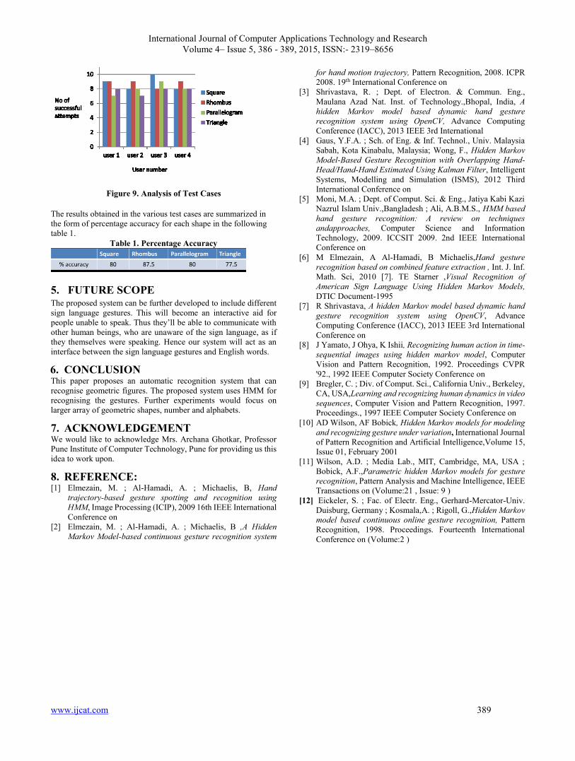
International Journal of Computer Applications Technology and Research
Volume 4– Issue 5, 386 - 389, 2015, ISSN:- 2319–8656
www.ijcat.com 389
Figure 9. Analysis of Test Cases
The results obtained in the various test cases are summarized in
the form of percentage accuracy for each shape in the following
table 1.
Table 1. Percentage Accuracy
5. FUTURE SCOPE The proposed system can be further developed to include different
sign language gestures. This will become an interactive aid for
people unable to speak. Thus they’ll be able to communicate with
other human beings, who are unaware of the sign language, as if
they themselves were speaking. Hence our system will act as an
interface between the sign language gestures and English words.
6. CONCLUSION This paper proposes an automatic recognition system that can
recognise geometric figures. The proposed system uses HMM for
recognising the gestures. Further experiments would focus on
larger array of geometric shapes, number and alphabets.
7. ACKNOWLEDGEMENT We would like to acknowledge Mrs. Archana Ghotkar, Professor
Pune Institute of Computer Technology, Pune for providing us this
idea to work upon.
8. REFERENCE: [1] Elmezain, M. ; Al-Hamadi, A. ; Michaelis, B, Hand
trajectory-based gesture spotting and recognition using
HMM, Image Processing (ICIP), 2009 16th IEEE International
Conference on
[2] Elmezain, M. ; Al-Hamadi, A. ; Michaelis, B ,A Hidden
Markov Model-based continuous gesture recognition system
for hand motion trajectory, Pattern Recognition, 2008. ICPR
2008. 19th International Conference on
[3] Shrivastava, R. ; Dept. of Electron. & Commun. Eng.,
Maulana Azad Nat. Inst. of Technology.,Bhopal, India, A
hidden Markov model based dynamic hand gesture
recognition system using OpenCV, Advance Computing
Conference (IACC), 2013 IEEE 3rd International
[4] Gaus, Y.F.A. ; Sch. of Eng. & Inf. Technol., Univ. Malaysia
Sabah, Kota Kinabalu, Malaysia; Wong, F., Hidden Markov
Model-Based Gesture Recognition with Overlapping Hand-
Head/Hand-Hand Estimated Using Kalman Filter, Intelligent
Systems, Modelling and Simulation (ISMS), 2012 Third
International Conference on
[5] Moni, M.A. ; Dept. of Comput. Sci. & Eng., Jatiya Kabi Kazi
Nazrul Islam Univ.,Bangladesh ; Ali, A.B.M.S., HMM based
hand gesture recognition: A review on techniques
andapproaches, Computer Science and Information
Technology, 2009. ICCSIT 2009. 2nd IEEE International
Conference on
[6] M Elmezain, A Al-Hamadi, B Michaelis,Hand gesture
recognition based on combined feature extraction , Int. J. Inf.
Math. Sci, 2010 [7]. TE Starner ,Visual Recognition of
American Sign Language Using Hidden Markov Models,
DTIC Document-1995
[7] R Shrivastava, A hidden Markov model based dynamic hand
gesture recognition system using OpenCV, Advance
Computing Conference (IACC), 2013 IEEE 3rd International
Conference on
[8] J Yamato, J Ohya, K Ishii, Recognizing human action in time-
sequential images using hidden markov model, Computer
Vision and Pattern Recognition, 1992. Proceedings CVPR
'92., 1992 IEEE Computer Society Conference on
[9] Bregler, C. ; Div. of Comput. Sci., California Univ., Berkeley,
CA, USA,Learning and recognizing human dynamics in video
sequences, Computer Vision and Pattern Recognition, 1997.
Proceedings., 1997 IEEE Computer Society Conference on
[10] AD Wilson, AF Bobick, Hidden Markov models for modeling
and recognizing gesture under variation, International Journal
of Pattern Recognition and Artificial Intelligence,Volume 15,
Issue 01, February 2001
[11] Wilson, A.D. ; Media Lab., MIT, Cambridge, MA, USA ;
Bobick, A.F.,Parametric hidden Markov models for gesture
recognition, Pattern Analysis and Machine Intelligence, IEEE
Transactions on (Volume:21 , Issue: 9 )
[12] Eickeler, S. ; Fac. of Electr. Eng., Gerhard-Mercator-Univ.
Duisburg, Germany ; Kosmala,A. ; Rigoll, G.,Hidden Markov
model based continuous online gesture recognition, Pattern
Recognition, 1998. Proceedings. Fourteenth International
Conference on (Volume:2 )

International Journal of Computer Applications Technology and Research
Volume 4– Issue 5, 390 - 394, 2015, ISSN:- 2319–8656
www.ijcat.com 390
Skip Graph in Distributed Environments: A Review
Upinder Kaur
Department of Computer Science and Application
Kurukshetra University
Kurukshetra, India
Pushpa Rani Suri
Department of Computer Science and Application
Kurukshetra University
Kurukshetra, India
Abstract: As we see that the world has become closer and faster and with the enormous growth of distributed networks like p2p,
social networks, overlay networks, cloud computing etc. Theses Distributed networks are represented as graphs and the
fundamental component of distributed network is the relationship defined by linkages among units or nodes in the network.
Major concern for computer experts is how to store such enormous amount of data especially in form of graphs. There is a need
for efficient data structure used for storage of such type of data should provide efficient format for fast retrieval of data as and
when required, in this types of networks. Although adjacency matrix is an effective technique to represent a graph having few or
large number of nodes and vertices but when it comes to analysis of huge amount of data from site likes like face book or twitter,
adjacency matrix cannot do this. In this paper, we study the existing application of a special kind of data structure, skip graph
with its various versions which can be efficiently used for storing such type of data resulting in optimal storage, space utilization
retrieval and concurrency.
Keywords: Skip List, Skip Graph, and Distributed Networks, Efficient and fast search
1 INTRODUCTION
1.1 SKIPLIST A skip list [3] is an ordered data structure based on a
succession of linked lists with geometrically
decreasing numbers of items. The deterministic
versions of skip list have
guaranteed properties whereas randomized skip lists
only offer high probability performance. This height
(Hn) is the maximum length of a search path for any
key from the top of the skip list. Devroye has proved
that this height Hn is of order log n [10].
Figure 1 - Example of Skip List [13]
1.2 SKIP GRAPH
The skip graph, introduced by Aspnes and Shah in [2, 4], is
a variant of the skip list, designed to perform better in a
distributed environment. In a skip graph, the whole data
structure can be distributed among a large number of nodes,
and the structure provides good load balancing and fault
tolerance properties.
As defined by author in [6] Skip graphs are data structures
with similar functionality to binary trees or skip lists,
permitting efficient insertion, removal and searches among
elements, but they are best suitable for P2P distributed
environments. Skip Graphs are composed of tower of
increasingly refined linked lists in various levels, each one
with no head and doubly linked. shown in fig from [6].
Skip graphs provide the full functionality of a balanced tree
in a distributed system where elements are stored in
separate nodes that may fall at any time as described in [3].
They are designed for use in searching peer-to-peer
networks, and by providing the ability to perform queries
based on key ordering, they improve on existing search
tools that provide only hash table functionality. As per analysis done by James and Shah in [2, 3] on skip lists or
other tree data structures, skip graphs are highly resilient,
tolerating a large fraction of failed nodes without losing
connectivity. In addition, constructing, inserting new
elements into, searching a skip graph and detecting and
repairing errors in the data structure introduced by node
failures can be done using simple and straightforward
algorithms. During past years interesting variants of skip

International Journal of Computer Applications Technology and Research
Volume 4– Issue 5, 390 - 394, 2015, ISSN:- 2319–8656
www.ijcat.com 391
graphs have been studied, like skip nets [7], skip webs [1]
or rainbow skip graphs [6].
Figure 2 - Example of Skip Graph [13]
2. MODELS AND NOTATIONS In a skip graph, each node represents a resource to be
searched where node x holds two fields: the first is a
key, which is arbitrary and may be the resource name.
Nodes are ordered according to their keys. For
notational convenience the keys are the considered to
be integers 1 , 2, . . . , n. Since the keys have no
function in the construction other than to provide an
ordering and a target for searches there is no loss of
generality. The second field is a membership vector
m(x) which is for convenience treated as an infinite
string of random bits chosen independently by each
node. In practice, it is enough to generate an O(log n)-
bit prefix of this string with overwhelming probability.
The nodes are ordered lexicographically by their keys
in a circular doubly-linked list
The insert operation
A new node „u‟ knows some introducing node „v‟ in
the network that will help it to join the network. Node
„u‟ inserts itself in one linked list at each level till it
finds itself in a singleton list at the topmost level. The
insert operation consists of two stages:
(1) Node „u‟ starts a search for itself from „v‟ to find
its neighbours at level 0, and links to them.
(2) Node „u‟ finds the closest nodes „s‟ and „y‟ at each level W _ 0, s < u < y, such that m(u) _
(W + 1) = m(s) & (W + 1) = m(y) _ (W + 1), if they
exist, and links to them at level W + 1. Because each
existing node „v‟ does not require m(v)(W+1) unless
there exists another node „u‟ such that m(v) _ (W + 1)
= m(u) _ (W + 1), it can delay determining its value
until a new node arrives asking for its value; thus at
any given time only a finite prefix of the membership
vector of any node needs to be generated.
The delete operation When node „u‟ wants to leave the
network, it deletes itself in parallel from all lists above
level 0 and then deletes itself from level 0.
3. SKIP GRAPH IN DIFFERENT
AREAS:
Skip index [15]: It is a distributed high-dimensional index
structure based on peer-to-peer overlay routing. A new
routing scheme is used to lookup data keys in the
distributed index, which guarantees logarithmic lookup and
maintenance cost, even in the face of skewed
datasets.efficient performance in dynamic load balancing
and handling complex queries.
Skip Webs [1]: Skip webs a framework for designing
randomized distributed data structure that improves
previous skip-graph/SkipNet approaches and extends their
area of applicability to multi-dimensional data sets. The
queries allowed include one-dimensional nearest neighbor
queries, string searching over fixed alphabets, and multi-
dimensional searching and point location. Our structure,
which we call skip-webs, matches the O(log n/ log log n)
expected query time of NoN skip-graphs [13, 14] for one-
dimensional data, while maintaining the O(log n) memory
size and expected query cost of traditional skip graphs [3]
and SkipNet [10]. We also introduce a bucketed version of
our skip-web structure, which improves the overall space
bounds of our structure, while also significantly improving
the expected query and update times.
Rainbow Skip Graph [8]: this is the first peer-to-peer data
structure that simultaneously achieves high fault-tolerance,
constant-sized nodes, and fast update and query times for
ordered data. It supports successor queries on a set of n
items using O(log n) messages with high probability, an
improvement over the expected O(log n) messages of the
family tree. The structure should be able to adjust to the
failure of some nodes, repairing the structure at small cost
in such casesThe structure should support fast queries and
insertions/deletions, in terms of the number of rounds of
communication and number of messages that must be
exchanged in order to complete requested operationsThe
structure should support queries that are based on an
ordering of the data, such as nearest-neighbor searches and
range queries.
Inverted skip graph [16] : Inverted skip graphs are
capable of processing mobile node updates within the skip
graph with fewer skip graph messages. In a 10,000 node
network, inverted skip graphs process a mobile node's
position update using a fourth of the messages (on average)
International Journal of Computer Applications Technology and Research
Volume 4– Issue 5, 390 - 394, 2015, ISSN:- 2319–8656
www.ijcat.com 392
a standard skip graph requires for the same task. When a
node changes geographical locations in the context of a
standard skip graph, a query is required to re-assign the
node in the proper position in the base list in Lo. inverted
skip graph outperforms the standard skip graph, mobility
performance and query execution,
SkipNet [12]: SkipNet also employs a background
stabilization mechanism that gradually updates all
necessary routing table entries when a node fails. Any
query to a live, reachable node will still succeed during this
time; the stabilization mechanism simply restores optimal
routing Performing range queries in SkipNet is therefore
equivalent to routing along the corresponding ring segment.
Because our current focus is on SkipNet‟s architecture and
locality properties, we do not discuss the use of range
queries for implementing various higher-level data query
operator
Skip Graphs++ [17] : Skip Graphs++ takes the
heterogeneity of P2P networks into account. It treats the
nodes differently and in Skip Graphs++ loads of nodes are
proportional to capacities of nodes. Powerful nodes afford
more loads and weak nodes afford fewer loads. Skip
Graphs++ may be a good tradeoff. The node starts the
search from its own search table, which will avoid the
problem of single point failure. The total number of the
node‟s pointers is proportional to the capacity of the node.
It will be easier to achieve better load balance
SkipStream [14]: SkipStream, a skip graph based Peer-to-
Peer (P2P) on-demand streaming scheme with VCR
support to on-demand streaming services with VCR
functionality over ubiquitous environments address the
above challenges. In the design of SkipStream, we first
group users into a set of disjoint clusters in accordance with
their playback offset and further organize the resulted
clusters into a skip graph based overlay network.. It is a
distributed on-demand streaming scheduling mechanism to
minimize the impact of VCR operations and balance
system load among nodes adaptively. The average search
latency of SkipStream is O (log (N ) ) where N is the
number of disjoint clusters. We also evaluate the
performance of SkipStream via extensive simulations.
Experimental results show that SkipStream outperforms
early skip list based scheme DSL by reducing the search
latency 20%-60% in average case and over 50% in worst
case.
Skip mard [18]: A new multi-attribute P2P resource
discovery approach (SkipMard) that extends Skip Graph
structure to support multi-attribute queries. SkipMard
provides a prefix matching resource routing algorithm to
resolve multi-attribute queries, and introduces the concepts
of “layer” and “crossing layer nearest neighbor” into the
data structure. To decrease message passing numbers, an
approximate closest-point method is addressed that can
help routing a searching key to a node with a key value that
has the minimum distance between two keys. Each node
has O(m*l) neighbors for total m layers and l levels in
SkipMard. The expected time for a multi-attribute query is
O(log N) and the message passing number is O(log
N)+O(k)
Table 1. Table showing the various Skip Graph
Applications.
3.1 BENEFITS OF SKIP GRAPHS
IN DIFFERENT APPLICATIONS
Correctness under concurrency
As discussed in section 2, both insertion and
deletion can be comfortably done on skip
graph and search operations eventually find
their target node or correctly report that it is
not present in the skip graph. So any search
operation can be linearized with respect to
insertion and deletion. In effect, the skip
graph inherits the atomicity properties of its
bottom layer, with upper layers serving only
to provide increased efficiency.
Concurrency is not handled properly in
various applications.
Fault Tolerance
Rainbow skip graph provides fault tolerance
properties of a skip graph [4]. Fault
tolerance of related data structures, such as
augmented versions of linked lists and
binary trees, has been well-studied by
Munro and Poblete [11]. The main question
is how many nodes can be separated from
the primary component by the failure of
other nodes, as this determines the size of
the surviving skip graph after the repair
mechanism finishes. It has been clearly
proved that even a worst-case choice of
failures by an adversary can do only limited
damage to the structure of the skip graph.
With high probability, a skip graph with n
nodes has an tQ(1/logn) expansion ratio,
implying that at most O(flog n) nodes can be
separated .

International Journal of Computer Applications Technology and Research
Volume 4– Issue 5, 390 - 394, 2015, ISSN:- 2319–8656
www.ijcat.com 393
Random failures
Rainbow skip graph, skipmards, skip webs
and skip nets efficiently handles random
failures, the situation appears even more
promising, experimental results presented in
[4,7,9] show that for a reasonably large skip
graph nearly all nodes remain in the primary
component until about two-thirds of the
nodes fail, and that it is possible to make
searches highly resilient to failure even
without using the repair mechanism by use
of redundant links.
Fast Search and Fault Tolerance
All the application of skip graph effienclty
works for fast searching and fault tolerance.
The average search in skip graph involves
only O(logn) nodes that most searches
succeed as long as the proportion of failed
nodes is substantially less than O(logn)
[1,8,9] . By detecting failures locally and
using additional redundant edges, one can
make searches highly tolerant to small
numbers of random faults. In general, results
cannot make as strong guarantees as those
provided by data structures based on explicit
use of expanders [6,7], but this is
compensated for by the simplicity of skip
graphs and the existence of good distributed
mechanisms for constructing and repairing
them
Load balancing
skip index, skip graph++, inverted skip
graphs are best suitable application for load
balancing in didtributed networks like p2p.
In addition to fault-tolerance, a skip graph
provides a limited form of load balancing,
by smoothing out hot spots caused by
popular search targets. The guarantees that a
skip graph makes in this case are similar to
the guarantees made for survivability. Just
as an element stored at a particular node will
not survive the loss of that node or its
neighbours in the graph, many searches
directed at a particular element will lead to
high load on the node that stores it and on
nodes likely to be on a search path.
However, James has shown that this effect
drops off rapidly with distance elements that
are far away from a popular target in the
bottom-level list produce little additional
load on average [4]. Further author has
provided two characterizations of this result.
The first shows that the probability that a
particular search uses a node between the
source and target drops off inversely with
the distance from the node to the target. This
fact is not necessarily reassuring to heavily-
loaded nodes. Since the probability averages
over all choices of membership vectors, it
may be that some particularly unlucky node
finds itself with a membership vector that
puts it on nearly every search path to some
very popular target. Second characterization
addresses load balancing issue by showing
that most of the load-spreading effects are
the result of assuming a random membership
vector for the source of the search.
Low hitting times
skip streams provides Random walks on
expanders done in [7] have the property of
hitting a large set of nodes fast and with high probability. This can be used for a
variety of applications such as load
balancing, gathering statistics on the nodes
of the skip graph and for finding highly
replicated.
High dimensional searching and range
queries
Skip index, rainbow skip graph, skip
streams, all provides a distributed high-
dimensional index structure based on peer-
to-peer overlay routing. A new routing
scheme is used to lookup data keys in the
distributed index, which guarantees
logarithmic lookup and maintenance cost,
even in the face of skewed datasets.efficient
performance in dynamic load balancing and
handling complex and range queries.
4. CONCLUSIONS AND FUTURE
SCOPE A short survey of skip graph with various application areas
provided in this paper, clearly indicate the usage and
advantages of using skip graphs in various distributed and
graph based applications. Since skip graphs provide the full
functionality of a balanced tree in a distributed system they
can be designed for use in searching peer-to-peer networks,
and by providing the ability to perform queries based on

International Journal of Computer Applications Technology and Research
Volume 4– Issue 5, 390 - 394, 2015, ISSN:- 2319–8656
www.ijcat.com 394
key ordering, they improve on existing search tools that
provide only hash table functionality. There are still many
unexplored areas where skip graphs can fine many useful
applications and one such application concurrent execution
of skip graph in distributed networks. Skip graphs can be
used to store the data in graphs and cluster the data and
above all retrieval will be very efficient and fast.
5. REFERENCES
[1] L. Arge, D. Eppstein, and M.T. Goodrich. Skip-
webs: efficient distributed data structures for multi-
dimensional data sets. Proceedings of the annual
ACM SIGACT-SIGOPS symposium on Principles of
distributed computing, pages 69–76, 2009.
[2] J. Aspnes and G. Shah. Skip graphs. Proceedings
of the fourteenth annual ACM-SIAM symposium on
Discrete algorithms, pages 384– 393, 2003.
[3] James Aspnes and Gauri Shah. Skip graphs. ACM
Transactions on Algorithms, 3(4):37, November
2007.
[4] James Aspnes and Udi Wieder. The expansion
and mixing time of skip graphs with applications. In
SPAA ‟05: Proceedings of the seventeenth annual
ACM symposium on Parallelism in algorithms and
architectures, pages 126–134, New York, NY, USA,
2005. ACM.
[5] Thomas Clouser, Mikhail Nesterenko, Christian
Scheideler : Tiara: A self-stabilizing deterministic
skip list and skip graph . 2012 Elsevier
[6] Hammurabi Mendes , Cristina G. Fernandes - A
Concurrent Implementation of Skip graphs .
Electronic Notes in Discrete Mathematics 35 (2009 )
page no .-263-268 .
[7] James Aspnes , Udi Wieder -The expansion and
mixing time of skip graphs with applications. page no
385-394 , Springer-Verlag 2008
[8] Michael T. Goodrich, Michael J. Nelson ,
Jonathan Z. Sun –The Rainbow Skip Graph: A Fault-
Tolerant Constant-Degree P2P Relay Structure .
ArXiv - 2009
[9] Fuminori Makikawa, Tatsuhiro Tsuchiya, Tohru
Kikuno – Balance and Proximity-Aware Skip Graph
Construction. 2010 First International Conference on
Networking and Computing .
10] Shabeera T P, Priya Chandran, Madhu Kumar S
D - Authenticated and Persistent Skip Graph: A Data
Structure for Cloud Based Data-Centric Applications
. CHENNAI, India , 2012 , ACM
[11] Ian Munro and Patricio V. Poblete. Fault
tolerance and storage reduction in binary search trees.
Information and Control, 62(2/3):210-218, August
1984.
[12] Jianjun Yu, Hao Su, Gang Zhou, Ke Xu - SNet:
Skip Graph based Semantic Web Services Discovery
. Seoul, Korea. 2007 ACM
[13] James Aspnes, Guari Shah, ppt in SODA 2003."
http://www.cs.yale.edu/homes/aspnes/papers/skip-
graphs-soda03.ppt"
[14] Qifeng Yu, Tianyin Xu, Baoliu Ye, Sanglu Lu
and Daoxu Chen. SkipStream: A Clustered Skip
Graph Based On-demand Streaming Scheme over
Ubiquitous Environments. Proceedings of IC-
BNMT2009, IEEE
[15] Chi Zhang Arvind Krishnamurthy Randolph Y.
Wang, SkipIndex: Towards a Scalable Peer-to-Peer
Index Service for High Dimensional Data. Vol ol.
TR-703-04 (May 2004)
[16] Gregory J. Brault', Christopher J. Augeri2, Barry
E. Mullins2, Christopher B. Mayer2, Rusty 0.
Baldwin,. Assessing Standard and Inverted Skip
Graphs Using Multi-Dimensional Range Queries and
Mobile Nodes, MobiQuitous 2007. Fourth Annual
International Conference on 6-10 Aug. 2007
[17] Wu Hengkui, Lin Fuhong, Zhang Hongke.
reducing maintenance overhead via heterogeneity in
skip graphs proceedings of ic-bnmt2009 ,2009 ieee
[18] Jun Ni ; Segre, A.M. ; Shaowen Wang.
SkipMard: a multi-attribute peer-to-peer resource
discovery approach. IMSCCS '07 Proceedings of the
Second International Multi-Symposiums on
Computer and Computational Sciences. 2007. IEEE

International Journal of Computer Applications Technology and Research
Volume 4– Issue 5, 395 - 404, 2015, ISSN:- 2319–8656
www.ijcat.com 395
Human Iris Recognition Using Linear Discriminant
Analysis Algorithm
Gafar Zen Alabdeen Salh
Department of IT
Faculty of Computers and IT
University of Jeddah, Khulais
Jeddah, Saudi Arabia
Abdelmajid Hassan Mansour
Department of IT
Faculty of Computers and IT
University of Jeddah, Khulais
Jeddah, Saudi Arabia
Elnazier Abdallah Mohammed
Department of CS
Faculty of CS and IT
Kassala University
Kassala, Sudan
Abstract: The paper holding a presentation of a system, which is recognizing peoples through their iris print and that by using Linear
Discriminant Analysis method. Which is characterized by the classification of a set of things in groups, these groups are observing a
group the features that describe the thing, and is characterized by finding a relationship which give rise to differences in the
dimensions of the iris image data from different varieties, and differences between the images in the same class and are less. This
Prototype proves a high efficiency on the process of classifying the patterns, the algorithms was applied and tested on MMU database,
and it gives good results with a ratio reaching up to 74%.
Keywords: linear discriminant analysis, iris recognition, Biometrics, False Rejection Rate, False Acceptance Rate
1. INTRODUCTION Biometrics refers to the identification of human identity via
special physiological traits. So scientists have been trying to
find solution for designing technologies that can analysis
those traits and ultimately distinguish between different
people. Some of popular Biometric characteristic are features
in fingerprint, speech, DNA, face and different part of it and
hand gesture. Among those method face recognition and
speaker recognition have been considered more than other
during last 2 decades [1].
Iris recognition is one of the most promising approach due to
its high reliability for personal identification. The human iris,
which is the annular part between the pupil and the white
sclera, has a complex pattern. The iris pattern is unique to
each person and to each eye and is essentially stable over a
lifetime. Also iris pattern of left and right eye is different.
Uniqueness, stability makes iris recognition a particularly
promising solution to security [3].
The iris is a thin diaphragm, which lies between the cornea
and the lens of the human eye. A front on view of iris is
shown in fig.1. The iris is perforated close to its centre by a
circular aperture known as pupil. The function of the iris is to
control the amount of light entering through the pupil. The
average diameter of the iris is 12mm and the pupil size can
vary from 10% to 80% of the iris diameter [2].
Iris patterns become interesting as an alternative approach to
reliable visual recognition of persons when imaging can be
done at distances of less than a meter, and especially when
there is a need to search very large databases without
incurring any false matches despite a huge number of
possibilities. Although small (11 mm) and sometimes
problematic to image, the iris has the great mathematical
advantage that its pattern variability among different persons
is enormous. In addition, as an internal (yet externally visible)
organ of the eye, the iris is well protected from the
environment and stable over time. As a planar object its image
is relatively insensitive to angle of illumination, and changes
in viewing angle cause only affine transformations; even the
nonaffine pattern distortion caused by pupillary dilation is
readily reversible. Finally, the ease of localizing eyes in faces,
and the distinctive annular shape of the iris, facilitate reliable
and precise isolation of this feature and the creation of a size-
invariant representation [7].
Fig 1: The Human Iris. [12]
In view of iris recognition issue, domestic and overseas
scholars have done a lot of in-depth researches, and put
forward many effective iris recognition methods. Iris image
has high dimensionality, and its feature dimensions often
exceed the number of samples, so that the iris image is sparse
in high-dimensional spatial distribution. If the original
features of iris image are directly entered into the classifier for

International Journal of Computer Applications Technology and Research
Volume 4– Issue 5, 395 - 404, 2015, ISSN:- 2319–8656
www.ijcat.com 396
learning, in which the useless and redundant features
adversely affect the iris image' recognition rate, resulting in
low identify efficiency [4], [5]. In order to solve the “curse of
dimensionality” and small sample size issues incurred by iris's
high-dimensional feature and improve the iris recognition rate
and efficiency, some scholars have proposed the sub-mode-
based iris recognition algorithm [4], [6]. Sub-mode-based iris
recognition algorithm refers to project the high-dimensional
iris image onto the low-dimensional subspace by adopting
certain dimensionality reduction methods, eliminate the
useless and redundant features, and extract the iris features in
low-dimensional spaces. Currentiris feature dimensionality
reduction techniques consists of the Principal Component
Analysis (PCA), Independent Component Analysis (ICA),
Linear Discriminant Analysis (LDA), Isometric Feature
Mapping (ISOMAP), Locally Linear Embedding algorithm
(LLE), Laplacian Eigenmap algorithm (LE), Locality
Preserving Projection (LPP) and so on. PCA, ICA, LDA are a
class of linear dimension reduction method, which can only
extract the global low-dimensional features. It is difficult to
find the nonlinear manifold [4].
2. Overview of Linear Discriminant
Analysis (LDA) : Linear Discriminant Analysis is a well-known scheme for
feature extraction and dimension reduction. It has been used
widely in many applications such as face recognition, image
retrieval, microarray data classification, etc. Classical LDA
projects the data onto a lower-dimensional vector space such
that the ratio of the between-class distance to the within-class
distance is maximized, thus achieving maximum
discrimination. The optimal projection (transformation) can
be readily computed by applying the Eigen decomposition on
the scatter matrices. An intrinsic limitation of classical LDA is
that its objective function requires the nonsingularity of one of
the scatter matrices. For many applications, such as face
recognition, all scatter matrices in question can be singular
since the data is from a very high-dimensional space, and in
general, the dimension exceeds the number of data points.
Given a data matrix A ∈ IRN×n, classical LDA aims to find a
transformation that maps each column ai of A, for
1 ≤ i ≤ n, in the N-dimensional space to a vector bi in the -
dimensional space. That is
. Equivalently,
classical LDA aims to find a vector space G spanned by
, such that each ai is
projected onto .
Assume that the original data in A is partitioned into k classes
as A = {Π1,···,Πk}, where
Πi contains ni data points from the ith class, and
. Classical LDA aims to find the optimal
transformation G such that the class structure of the original
high-dimensional space is preserved in the low-dimensional
space.
In general, if each class is tightly grouped, but well separated
from the other classes, the quality of the cluster is considered
to be high. In discriminant analysis, two scatter matrices,
called within-class (Sw) and between-class (Sb) matrices, are
defined to quantify the quality of the cluster, as follows [4]:
, and
, where
is the mean of the ith class,
And is the global mean.
It is easy to verify that trace(Sw) measures the closeness of
the vectors within the classes, while trace(Sb) measures the
separation between classes. In the low-dimensional space
resulting from the linear transformation G (or the linear
projection onto the vector space G), the within-class and
between-class matrices become SbL = GTSbG, and SwL =
GTSwG.
An optimal transformation G would maximize trace(SbL) and
minimize trace(SwL). Common optimizations in classical
discriminant analysis:
and trace .
(1)
The optimization problems in Eq. (1) are equivalent to the
following generalized eigenvalue problem:
. The solution can be obtained by
applying an Eigen decomposition to the matrix Sw−1Sb, if Sw is
nonsingular, or Sb−1Sw, if Sb is nonsingular. There are at most k
− 1 eigenvectors corresponding to nonzero eigenvalues, since
the rank of the matrix Sb is bounded from above by k − 1.
Therefore, the reduced dimension by classical LDA is at most
k − 1. A stable way to compute the eigen-decomposition is to
apply SVD on the scatter matrices. Details can be found in
[14].
3. RELATED WORK John Daugman [10] presents the statistical variability that is
the basis of iris recognition is analyzed, using new large
databases. The principle underlying the recognition algorithm
is the failure of a test of statistical independence on iris phase
structure encoded by multi-scale quadrature wavelets.
Combinatorial complexity of this phase information across
deferent persons spans about 249 degrees-of-freedom and
generates a discrimination entropy of about 3:2 bits=mm2
over the iris, enabling real-time identi/cation decisions with
great enough accuracy to support exhaustive searches through
very large databases. This paper presents the results of 9.1
million comparisons among several thousand eye images
acquired in trials in Britain, the USA, Japan and Korea.? 2002
Pattern Recognition Society. Published by Elsevier Science
Ltd. All rights reserved. Shideh Homayon , [1] proposes
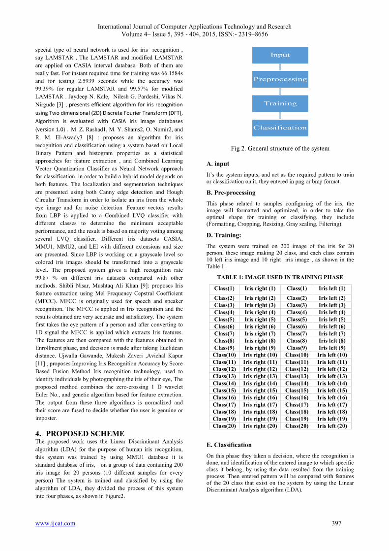
International Journal of Computer Applications Technology and Research
Volume 4– Issue 5, 395 - 404, 2015, ISSN:- 2319–8656
www.ijcat.com 397
special type of neural network is used for iris recognition ,
say LAMSTAR , The LAMSTAR and modified LAMSTAR
are applied on CASIA interval database. Both of them are
really fast. For instant required time for training was 66.1584s
and for testing 2.5939 seconds while the accuracy was
99.39% for regular LAMSTAR and 99.57% for modified
LAMSTAR . Jaydeep N. Kale, Nilesh G. Pardeshi, Vikas N.
Nirgude [3] , presents efficient algorithm for iris recognition
using Two dimensional (2D) Discrete Fourier Transform (DFT),
Algorithm is evaluated with CASIA iris image databases
(version 1.0) . M. Z. Rashad1, M. Y. Shams2, O. Nomir2, and
R. M. El-Awady3 [8] : proposes an algorithm for iris
recognition and classification using a system based on Local
Binary Pattern and histogram properties as a statistical
approaches for feature extraction , and Combined Learning
Vector Quantization Classifier as Neural Network approach
for classification, in order to build a hybrid model depends on
both features. The localization and segmentation techniques
are presented using both Canny edge detection and Hough
Circular Transform in order to isolate an iris from the whole
eye image and for noise detection .Feature vectors results
from LBP is applied to a Combined LVQ classifier with
different classes to determine the minimum acceptable
performance, and the result is based on majority voting among
several LVQ classifier. Different iris datasets CASIA,
MMU1, MMU2, and LEI with different extensions and size
are presented. Since LBP is working on a grayscale level so
colored iris images should be transformed into a grayscale
level. The proposed system gives a high recognition rate
99.87 % on different iris datasets compared with other
methods. Shibli Nisar, Mushtaq Ali Khan [9]: proposes Iris
feature extraction using Mel Frequency Cepstral Coefficient
(MFCC). MFCC is originally used for speech and speaker
recognition. The MFCC is applied in Iris recognition and the
results obtained are very accurate and satisfactory. The system
first takes the eye pattern of a person and after converting to
1D signal the MFCC is applied which extracts Iris features.
The features are then compared with the features obtained in
Enrollment phase, and decision is made after taking Euclidean
distance. Ujwalla Gawande, Mukesh Zaveri ,Avichal Kapur
[11] , proposes Improving Iris Recognition Accuracy by Score
Based Fusion Method Iris recognition technology, used to
identify individuals by photographing the iris of their eye, The
proposed method combines the zero-crossing 1 D wavelet
Euler No., and genetic algorithm based for feature extraction.
The output from these three algorithms is normalized and
their score are fused to decide whether the user is genuine or
imposter.
4. PROPOSED SCHEME The proposed work uses the Linear Discriminant Analysis
algorithm (LDA) for the purpose of human iris recognition,
this system was trained by using MMU1 database it is
standard database of iris, on a group of data containing 200
iris image for 20 persons (10 different samples for every
person) The system is trained and classified by using the
algorithm of LDA, they divided the process of this system
into four phases, as shown in Figure2.
Fig 2. General structure of the system
A. input
It’s the system inputs, and act as the required pattern to train
or classification on it, they entered in png or bmp format.
B. Pre-processing
This phase related to samples configuring of the iris, the
image will formatted and optimized, in order to take the
optimal shape for training or classifying, they include
(Formatting, Cropping, Resizing, Gray scaling, Filtering).
D. Training:
The system were trained on 200 image of the iris for 20
person, these image making 20 class, and each class contain
10 left iris image and 10 right iris image , as shown in the
Table 1.
TABLE 1: IMAGE USED IN TRAINING PHASE
Class(1) Iris right (1) Class(1) Iris left (1)
Class(2) Iris right (2) Class(2) Iris left (2)
Class(3) Iris right (3) Class(3) Iris left (3)
Class(4) Iris right (4) Class(4) Iris left (4)
Class(5) Iris right (5) Class(5) Iris left (5)
Class(6) Iris right (6) Class(6) Iris left (6)
Class(7) Iris right (7) Class(7) Iris left (7)
Class(8) Iris right (8) Class(8) Iris left (8)
Class(9) Iris right (9) Class(9) Iris left (9)
Class(10) Iris right (10) Class(10) Iris left (10)
Class(11) Iris right (11) Class(11) Iris left (11)
Class(12) Iris right (12) Class(12) Iris left (12)
Class(13) Iris right (13) Class(13) Iris left (13)
Class(14) Iris right (14) Class(14) Iris left (14)
Class(15) Iris right (15) Class(15) Iris left (15)
Class(16) Iris right (16) Class(16) Iris left (16)
Class(17) Iris right (17) Class(17) Iris left (17)
Class(18) Iris right (18) Class(18) Iris left (18)
Class(19) Iris right (19) Class(19) Iris left (19)
Class(20) Iris right (20) Class(20) Iris left (20)
E. Classification
On this phase they taken a decision, where the recognition is
done, and identification of the entered image to which specific
class it belong, by using the data resulted from the training
process. Then entered pattern will be compared with features
of the 20 class that exist on the system by using the Linear
Discriminant Analysis algorithm (LDA).

International Journal of Computer Applications Technology and Research
Volume 4– Issue 5, 395 - 404, 2015, ISSN:- 2319–8656
www.ijcat.com 398
V. RESULTS OF TESTING THE SYSTEM ON
MMU1 DATABASE OF IRIS
The Multimedia University has developed a small data set of
450 iris images (MMU). They was captured through one of
the most common iris recognition cameras presently
functioning (LG Iris Access 2200). This is a semi-automated
camera that operates at the range of 7-25 cm. Further, a new
data set (MMU2) comprised of 995 iris images has been
released and another common iris recognition camera
(Panasonic BM-ET100US Authenticam) was used. The iris
images are from 100 volunteers with different ages and
nationalities. They come from Asia, Middle East, Africa and
Europe and each of them contributed with five iris images
from each eye. [15]
The test was over twenty people and each person has ten iris
images under different illuminations and distances from the
camera.
I. Recognition of group 1 After testing the image of the group number 1, the system was
recognized to 8 sample out of 10, as shown in the Table 2
and Fig 3.
Table 2: RECOGNITION OFGROUP 1
Frequency Percent
Valid
Percent
Valid false
Classification 2 20.0 20.0
True
Classification 8 80.0 80.0
Total 10 100.0 100.0
Fig 3. Recognition of group 1
II. Recognition of group 2 After testing the image of the group number 2, the system was
recognized to 8 sample out of 10, as shown in the Table 3
and Fig 4.
Table 3: RECOGNITION OFGROUP 2
Frequency Percent
Valid
Percent
Valid false
Classification 2 20.0 20.0
True
Classification 8 80.0 80.0
Total 10 100.0 100.0
Fig4. Recognition of group 2
III. Recognition of group 3 After testing the image of the group number 3, the system was
recognized to 9 sample out of 10, as shown in the Table 4 and
Fig 5.
Table 4: RECOGNITION OFGROUP 3
Frequency Percent
Valid
Percent
Valid false
Classification 1 10.0 10.0
True
Classification 9 90.0 90.0
Total 10 100.0 100.0
Fig 5. Recognition of group 3
IV. A. Recognition of group 4 After testing the image of the group number 4, the system was
recognized to 8 sample out of 10, as shown in the Table 5 and
Fig 6.
Table 5: RECOGNITION OFGROUP 4
Frequency Percent
Valid
Percent
Valid false
Classification 2 20.0 20.0
True
Classification 8 80.0 80.0
Total 10 100.0 100.0
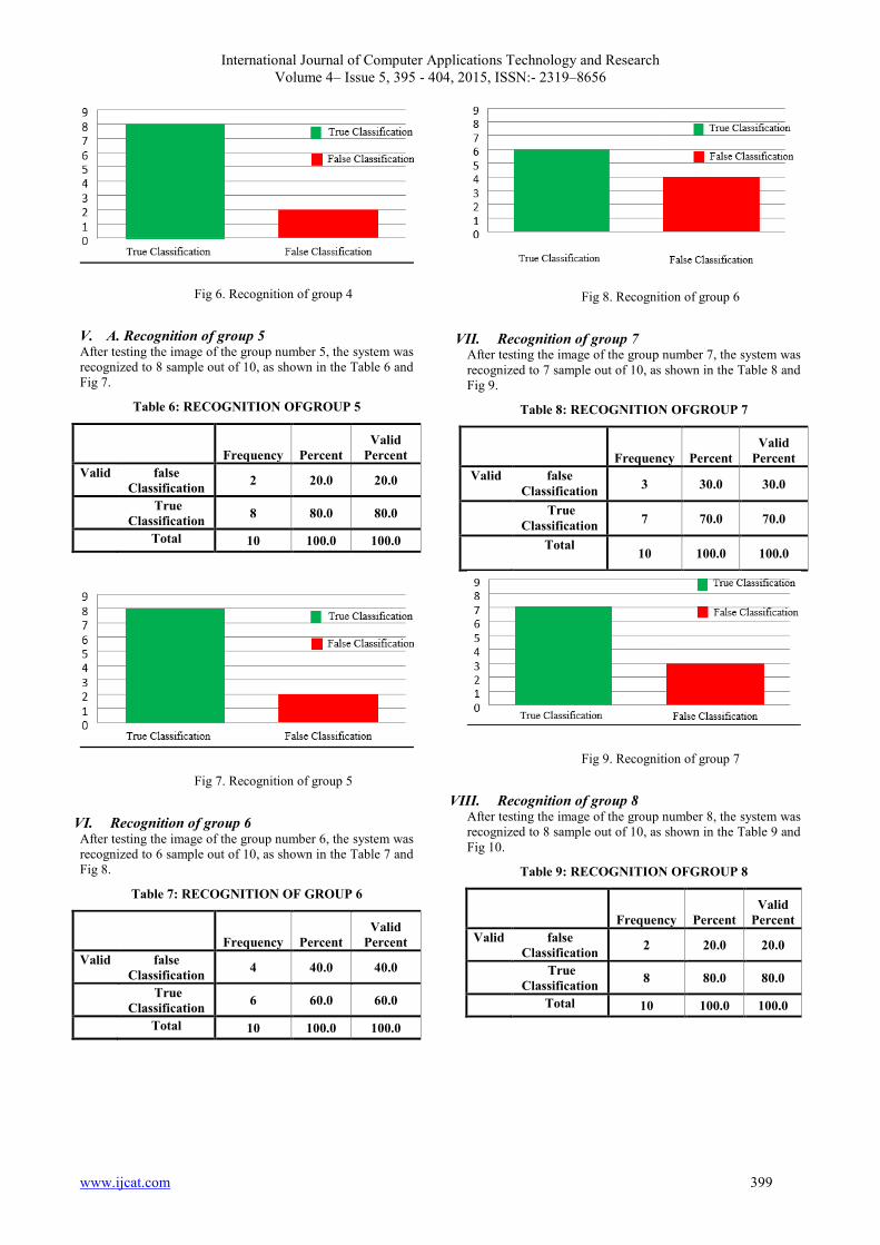
International Journal of Computer Applications Technology and Research
Volume 4– Issue 5, 395 - 404, 2015, ISSN:- 2319–8656
www.ijcat.com 399
Fig 6. Recognition of group 4
V. A. Recognition of group 5 After testing the image of the group number 5, the system was
recognized to 8 sample out of 10, as shown in the Table 6 and
Fig 7.
Table 6: RECOGNITION OFGROUP 5
Frequency Percent
Valid
Percent
Valid false
Classification 2 20.0 20.0
True
Classification 8 80.0 80.0
Total 10 100.0 100.0
Fig 7. Recognition of group 5
VI. Recognition of group 6 After testing the image of the group number 6, the system was
recognized to 6 sample out of 10, as shown in the Table 7 and
Fig 8.
Table 7: RECOGNITION OF GROUP 6
Frequency Percent
Valid
Percent
Valid false
Classification 4 40.0 40.0
True
Classification 6 60.0 60.0
Total 10 100.0 100.0
Fig 8. Recognition of group 6
VII. Recognition of group 7 After testing the image of the group number 7, the system was
recognized to 7 sample out of 10, as shown in the Table 8 and
Fig 9.
Table 8: RECOGNITION OFGROUP 7
Frequency Percent
Valid
Percent
Valid false
Classification 3 30.0 30.0
True
Classification 7 70.0 70.0
Total 10 100.0 100.0
Fig 9. Recognition of group 7
VIII. Recognition of group 8 After testing the image of the group number 8, the system was
recognized to 8 sample out of 10, as shown in the Table 9 and
Fig 10.
Table 9: RECOGNITION OFGROUP 8
Frequency Percent
Valid
Percent
Valid false
Classification 2 20.0 20.0
True
Classification 8 80.0 80.0
Total 10 100.0 100.0

International Journal of Computer Applications Technology and Research
Volume 4– Issue 5, 395 - 404, 2015, ISSN:- 2319–8656
www.ijcat.com 400
Fig 10. Recognition of group 8
IX. Recognition of group 9 After testing the image of the group number 9, the system was
recognized to 8 sample out of 10, as shown in the Table 10
and Fig 11.
Table 10: RECOGNITION OFGROUP 9
Frequency Percent
Valid
Percent
Valid false
Classification 2 20.0 20.0
True
Classification 8 80.0 80.0
Total 10 100.0 100.0
Fig 11. Recognition of group 9
X. Recognition of group 10 After testing the image of the group number 10, the system
was recognized to 8 sample out of 10, as shown in the Table
11 and Fig 12.
Table 11: RECOGNITION OFGROUP 10
Frequency Percent
Valid
Percent
Valid false
Classification 2 20.0 20.0
True
Classification 8 80.0 80.0
Total 10 100.0 100.0
Fig 12. Recognition of group 10
XI. Recognition of group 11 After testing the image of the group number 11, the system
was recognized to 7 sample out of 10, as shown in the Table
12 and Fig 13.
Table 12: RECOGNITION OFGROUP 11
Frequency Percent
Valid
Percent
Valid false
Classification 3 30.0 30.0
True
Classification 7 70.0 70.0
Total 10 100.0 100.0
Fig 13. Recognition of group 11
XII. Recognition of group 12 After testing the image of the group number 8, the system was
recognized to 7 sample out of 10, as shown in the Table 13
and Fig 14.
Table 13: RECOGNITION OFGROUP 12
Frequency Percent
Valid
Percent
Valid false
Classification 3 30.0 30.0
True
Classification 7 70.0 70.0
Total 10 100.0 100.0

International Journal of Computer Applications Technology and Research
Volume 4– Issue 5, 395 - 404, 2015, ISSN:- 2319–8656
www.ijcat.com 401
Fig 14. Recognition of group 12
XIII. Recognition of group 13 After testing the image of the group number 13, the system
was recognized to 7 sample out of 10, as shown in the Table
14 and Fig 15.
Table 14: RECOGNITION OFGROUP 13
Frequency Percent
Valid
Percent
Valid false
Classification 3 30.0 30.0
True
Classification 7 70.0 70.0
Total 10 100.0 100.0
Fig 15. Recognition of group 13
XIV. Recognition of group 14 After testing the image of the group number 14, the system
was recognized to 9 sample out of 10, as shown in the Table
15 and Fig 16.
Table 15: RECOGNITION OFGROUP 14
Frequency Percent
Valid
Percent
Valid false
Classification 1 10.0 10.0
True
Classification 9 90.0 90.0
Total 10 100.0 100.0
Fig 16. Recognition of group 14
XV. Recognition of group 15 After testing the image of the group number 15, the system
was recognized to 7 sample out of 10, as shown in the Table
16 and Fig 17.
Table 16: RECOGNITION OFGROUP 15
Frequency Percent
Valid
Percent
Valid false
Classification 3 30.0 30.0
True
Classification 7 70.0 70.0
Total 10 100.0 100.0
Fig 17. Recognition of group 15
XVI. Recognition of group 16 After testing the image of the group number 16, the system
was recognized to 7 sample out of 10, as shown in the Table
17 and Fig 18.
Table 17: RECOGNITION OFGROUP 16
Frequency Percent
Valid
Percent
Valid false
Classification 3 30.0 30.0
True
Classification 7 70.0 70.0
Total 10 100.0 100.0
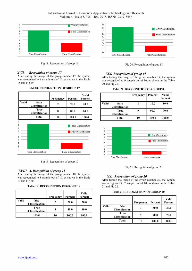
International Journal of Computer Applications Technology and Research
Volume 4– Issue 5, 395 - 404, 2015, ISSN:- 2319–8656
www.ijcat.com 402
Fig 18. Recognition of group 16
XVII. Recognition of group 17 After testing the image of the group number 17, the system
was recognized to 8 sample out of 10, as shown in the Table
18 and Fig 19.
Table18: RECOGNITION OFGROUP 17
Frequency Percent
Valid
Percent
Valid false
Classification 2 20.0 20.0
True
Classification 8 80.0 80.0
Total 10 100.0 100.0
Fig 19. Recognition of group 17
XVIII. A. Recognition of group 18 After testing the image of the group number 18, the system
was recognized to 8 sample out of 10, as shown in the Table
19 and Fig 20.
Table 19: RECOGNITION OFGROUP 18
Frequency Percent
Valid
Percent
Valid false
Classification 2 20.0 20.0
True
Classification 8 80.0 80.0
Total 10 100.0 100.0
Fig 20. Recognition of group 18
XIX. Recognition of group 19 After testing the image of the group number 19, the system
was recognized to 9 sample out of 10, as shown in the Table
20 and Fig 21.
Table 20: RECOGNITION OFGROUP 8
Frequency Percent Valid
Percent
Valid false
Classification
1 10.0 10.0
True
Classification
9 90.0 90.0
Total 10 100.0 100.0
Fig 21. Recognition of group 21
XX. Recognition of group 20 After testing the image of the group number 20, the system
was recognized to 7 sample out of 10, as shown in the Table
21 and Fig 22.
Table 21: RECOGNITION OFGROUP 20
Frequency Percent
Valid
Percent
Valid false
Classification 3 30.0 30.0
True
Classification 7 70.0 70.0
Total 10 100.0 100.0
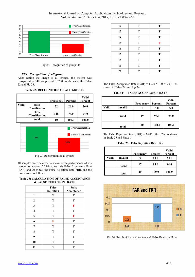
International Journal of Computer Applications Technology and Research
Volume 4– Issue 5, 395 - 404, 2015, ISSN:- 2319–8656
www.ijcat.com 403
Fig 22. Recognition of group 20
XXI. Recognition of all groups After testing the image of all groups, the system was
recognized to 148 sample out of 200, as shown in the Table
22 and Fig 23.
Table 22: RECOGNITION OF ALL GROUPS
Frequency Percent
Valid
Percent
Valid false
Classification 52 26.0 26.0
True
Classification 148 74.0 74.0
total 10 100.0 100.0
Fig 23. Recognition of all groups
40 samples were selected to measure the performance of iris
recognition system .20 iris to test iris False Acceptance Rate
(FAR) and 20 to test the False Rejection Rate FRR, and the
results were as follows:
Table 23: CALCULATION OF FALSE ACCEPTANCE
& FALSE REJECTION RATE
False
Rejection
False
Acceptance
1 T T
2 T T
3 T F
4 T T
5 T F
6 F T
7 T T
8 T T
9 T T
10 T T
11 T T
12 T T
13 T T
14 T T
15 T F
16 T T
17 T T
18 T T
19 T T
20 T T
The False Acceptance Rate (FAR) = 1 /20 * 100 = 5%, as
shown in Table 24 .and Fig 24.
Table 24: FALSE ACCEPTANCE RATE
Frequency Percent
Valid
Percent
Valid invalid 1 5.0 5.0
valid
19 95.0 94.0
total 20 100.0 100.0
The False Rejection Rate (FRR) = 3/20*100= 15%, as shown
in Table 25 and Fig 24.
Table 25: False Rejection Rate FRR
Frequency Percent
Valid
Percent
Valid invalid 3 15.0 5.01
valid 17 85.0 84.0
total 20 100.0 100.0
Fig 24. Result of False Acceptance & False Rejection Rate

International Journal of Computer Applications Technology and Research
Volume 4– Issue 5, 395 - 404, 2015, ISSN:- 2319–8656
www.ijcat.com 404
5. CONCULSION The paper aim to increase efficiently of iris recognition
process , which was reached recognition rate amounted to
74% , the samples are trained and tested on standard database
of iris (MMU), as we have acquired False Acceptance Rate,
FAR) is 5 %, a ratio less than the False Rejection Rate (FRR)
, which amounted to (15% )therefore, we can say that the
linear discriminate analysis algorithm (LDA ) highly efficient
in identifying the iris recognition .
6. References [1] Shideh Homayon, IRIS RECOGNITION FOR
PERSONAL IDENTIFICATION USING LAMSTAR
NEURALNETWORK , International Journal of
Computer Science & Information Technology (IJCSIT)
Vol 7, No 1, February 2015.
DOI:10.5121/ijcsit.2015.7101.
[2] Ms. Aparna G. Gale, DR. S. S. Salankar , A Review On
Advance Methods Of Feature Extraction In Iris
Recognition System, IOSR Journal of Electrical and
Electronics Engineering (IOSR-JEEE) e-ISSN: 2278-
1676, p-ISSN: 2320-3331 PP 65-70
www.iosrjournals.org , International Conference on
Advances in Engineering & Technology – 2014 (ICAET-
2014) 65 | Page
[3] Jaydeep N. Kale, Nilesh G. Pardeshi, Vikas N. Nirgude ,
Improved Iris Recognition using Discrete Fourier
Transform, International Journal of Computer
Applications (0975 – 8887) International Conference on
Recent Trends in engineering & Technology -
2013(ICRTET'2013)
[4] Yongqiang LI, Iris Recognition Algorithm based on
MMC-SPP ,International Journal of Signal Processing,
Image Processing and Pattern Recognition Vol. 8, No. 2
(2015),pp.1-10
http://dx.doi.org/10.14257/ijsip.2015.8.2.01
[5] Z. N. Sun and T. N.Tan,“Ordinal Measures for Iris
Recognition”,IEEE Trans. Pattern Analysis and Machine
Intelligence ,vol. 31, no. 12, (2009), pp.2211-2226.
[6] Z. HeandL. Lv, “Iris feature extraction and recognition
based on ICA-MJE and SVM”,Computer Applications,
vol.27, no. 6, (2007), pp.1505-1507.
[7] John Daugman, How Iris Recognition Works, IEEE
TRANSACTIONS ON CIRCUITS AND SYSTEMS
FOR VIDEO TECHNOLOGY, VOL. 14, NO. 1,
JANUARY 2004 .pp 21-30.
[8] M. Z. Rashad1, M. Y. Shams2, O. Nomir2, and R. M. El-
Awady3 ,IRIS RECOGNITION BASED ON LBP AND
COMBINED LVQ CLASSIFIER , International Journal
of Computer Science & Information Technology
(IJCSIT) Vol 3, No 5, Oct 2011, DOI :
10.5121/ijcsit.2011.3506
[9] Shibli Nisar, Mushtaq Ali Khan, Muhammad Usman ,
Iris Recognition using Mel Fequency Cepstral
Coefficient , International Journal of Engineering
Research (ISSN:2319-6890)(online),2347-5013(print)
Volume No.3, Issue No.2, pp : 100-103
[10] J. Daugman, “The importance of being random:
statistical principles of iris recognition”, Pattern
Recognition Society, Vol. 36, pp. 279-291, 2003.
[11] Ujwalla Gawande, Mukesh Zaveri ,Avichal Kapur ,
Improving Iris Recognition Accuracy by Score Based
Fusion Method , International Journal of Advancements
in Technology (IJoAT) http://ijict.org/ ISSN 0976-4860 ,
Vol 1, No 1 (June 2010) ©IJoAT .
[12] Sangini Shah, Ankita Mandowara, Mitesh Patel , IRIS
SEGMENTATION AND RECOGNITION FOR
HUMAN IDENTIFICATION, INTERNATIONAL
JOURNAL OF INNOVATIVE RESEARCH IN
TECHNOLOGY, © 2014 IJIRT | Volume 1 Issue 7 |
ISSN: 2349-6002
[13] VO Dinh Minh Nhat and SungYoung Lee (2007). Image-
based Subspace Analysis for Face Recognition, Face
Recognition, Kresimir Delac and Mislav Grgic (Ed.),
ISBN: 978-3-902613-03-5, InTech, Available
from:http://www.intechopen.com/books/face_recognition
/image-based_subspace_analysis_for_face_recognition
[14] J. Ye, R. Janardan, and Q. Li, “Two-dimensional linear
discriminant analysis,” Advances in Neural Information
Processing Systems (NIPS2004), 17:1569-1576, 2004.
[15] “MMU Iris Image Database: Multimedia University,”
http://pesona.mmu.edu.my/ccteo; 2004
Authors Profile
Dr. Gafar Zen Alabdeen Salh Hassan, Assistant Professor, Department of
Computers and Information Technology,
University of Jeddah, Faculty of
Computers and Information Technology,
Khulais, Jeddah, Saudi Arabia..
Permanent Address: Department of
Information Technology, Faculty of
computer Science and Information
Technology, Alneelain University, Khartoum, Sudan.
Dr. Abdelmajid Hassan Mansour Emam, Assistant Professor, Department of
Computers and Information Technology,
University of Jeddah, Faculty of
Computers and Information Technology,
Khulais, Jeddah, Saudi Arabia.
Permanent Address: Department of
Information Technology, Faculty of
computer Science and Information
Technology, Alneelain University, Khartoum, Sudan.
Elnazier Abdallah Mohammed Elhassan, Lecturer, Department of computer
Science, Faculty of computer Science
and Information Technology, Kassala
University , Kassala, Sudan

International Journal of Computer Applications Technology and Research
Volume 4– Issue 5, 405 - 408, 2015, ISSN:- 2319–8656
www.ijcat.com 405
Evaluation of automated web testing tools
Mohamed Monier
Information System Department,
Faculty of Computers and Informatics, Zagazig
University, Egypt.
Mahmoud Mohamed El-mahdy
Information System Department,
Faculty of Computers and Informatics, Zagazig
University, Egypt.
Abstract: Software testing is a main part of Software Development Life Cycle and one of the important aspects of Software
Engineering. There is a wide variety of testing tools which require or not the user experience in testing software products. According
to the daily use, Mobile and Web applications take the first place in development and testing. Testing automation enables developers
and testers to easily automate the entire process of testing in software development saving time and costs. This paper provide a
feasibility study for commercial and open source web testing tools helping developers or users to pick the suitable tool based on their
requirements.
Keywords: Black Box Testing; web testing tools; open source; Commercial;
1. INTRODUCTION Software Testing aims to evaluating the software quality and
to what degree the efficiency of that product. Testing Process
including many aspects such as reliability, usability, integrity,
maintainability and compatibility [1].
The Two main types of Software testing Black Box Testing
and White Box [2].Black Box Testing concerned with the
specification of the System component under test which not
require intensive knowledge about the internal structure of the
system. White box strategy otherwise require high experience
of the internal system code for developing test suits suited the
test cases.
Web and Mobile applications have become very complex and
crucial, Most of researches focused attention to Web
application design, development, analysis, and testing, by
studying and proposing methodologies and tools [3].Mobile
applications developed over more than platform which need
more experience in the developing environment and structure
of applications to be designed and developed.
Software Testing follow two ways manual or automation.
Manual Testing has many drawbacks such as consuming time
and cost, require experience, complex reusing, less efficiency
and not provide scripting facility for code [4].Automation
testing reveal all complex Obstacles attached with manual
testing, this type of testing create a scenarios by recording the
interaction with the system under design into test cases to be
tested under many Configurations [5].
Automated testing tools exist widely in the market varying in
the capabilities and features which make the user puzzled for
which tool suitable for his testing purpose [6]. There are two
types testing tools commercial and open source tools. Open
source tools are free for users to use with open source code to
be modified. On the other hand, Commercial tools take
advantage in organizations and mentoring capabilities
providing the user with facilities needed to accomplish tasks
with extra controlled features and low efforts.
The Objective of this paper is to present feasibility study of
automated web testing tools through comparing the tools
features for helping users to select suitable tools according to
their requirements based on a study of tool’s major criteria.
The paper divided into sections. Section I provide a brief
overview of testing tools. Section II discuss the tools features
and criteria used as input to the model. Section III discuss the
related work. Section IV Methodology Section V finally
provide the conclusion and future work.
2. RELATED WORK Last researches interested in comparing the capabilities of the
testing tools by practicing them or only based features each
tool support. Harpreet Kaur, Gagan Gupta conduct a
comparative study among selenium, Test Complete and QTP
tools the study include many aspects but not drag the
automation features of tools such as record and play-back,
cross platform or browsers support features [7]. Abha Jain,
Manish Jain, Sunil Dhankar[8] compare two commercial tools
Ranorex vs. QTP including many features but the main
concern on the cost of the total project and the study not
include any open source software to compare against. Angmo,
R and Sharma, M [9] compare the performance of selenium
web driver against watir-web driver the two open source
software, Study includes performance parameters such as
execution speed which vary in the type of tested Controls.
This research is efficient but require more than one tool to
give the best judge to the user.
3. METHODOLOGY There are a lot of web testing tools exist on the market
commercial or open source. We select the tools that perform
the automation testing using record scripts and then playback
this scripts as an important feature in testing automation.
3.1 Automated Software testing tools
3.1.1 Selenium webdriver Selenium IDE is a one of the most popular free open-source
automated testing tool which provide a testing framework for
testing web applications and supporting multiple kind of
frameworks. It can be easily downloaded from internet as a
plug-in for some browsers. It is basically used by the web
development community to perform automated testing of web
applications. We choose in our study Selenium web-driver
because Selenium IDE not support record-playback feature
and also it most supportive for web-application testing [10].

International Journal of Computer Applications Technology and Research
Volume 4– Issue 5, 405 - 408, 2015, ISSN:- 2319–8656
www.ijcat.com 406
3.1.2 Sahi Sahi is an open source provide a testing framework based on
Ruby and java script supporting the most types of web
browsers and platforms. Sahi provides powerful abilities for
recording and replaying across browsers; different language
drivers for writing test scripts (Java, Ruby) and support for
AJAX and highly dynamic web application Sahi used by IBM
developers for web applications testing automation [11].
3.1.3 Watir-web driver Watir is an abbreviation for Watir application testing in Ruby.
Is a powerful open source tool that requires programming
skills in ruby language [12].We choose Watir web-driver for
evaluation study in web automated testing as it support
record-playback capability. It is available as RubyGems and
capable of driving variety of browser including the major like
Internet Explorer, Firefox etc. [13]. Bret Pettichord and Paul
Rogers developed Watir. Watir project is composed of several
other projects of which watir-classic, watershed and watir
webdriver are important.
3.1.4 Quick Test Profession Quick Test Profession is an automated testing tools based on
graphical interface record playback capability [14]. It works
by identifying the objects in the application user interface or
web page and performing desired operations (such as mouse
and keyboard events).QTP uses a VBScript scripting language
to specify test procedures and manipulate activities.
Automated testing tool QTP provides the industry’s good
solution for functional test and regression test automation –
addressing every major software application and environment.
Quick Test Professional also enables testing Java applets and
applications, and multimedia objects on Applications as well
as standard Windows applications, It works by identifying the
objects in the application user interface or a web page and
performing desired operations (such as mouse clicks or
keyboard events); it can also capture objects properties [15].
3.1.5 Ranorex Ranorex is a commercial and complete image-based detection
tool used for programmed testing [16]. Ranorex perform
testing based on Image detection and facility to record and
playback. It does not necessitate to study a scripting language,
since it is written in pure .net code using C#, VB.net and Iron
Python. Ranorex recommended for expanded projects with
new license for tools as it cost benefits but the support
restricted only to companies.
3.1.6 Test Complete TestComplete is a testing automation tool formulated as Smart
Bear testing framework [17]. It makes available the testing of
windows and web applications and is one of the primary
functional testing tools in the world. TC is a graphical record-
playback automation tool which supports various testing types
and methodologies: unit testing, functional and GUI testing,
regression testing, distributed testing.TC provide recording
and capabilities of generation of test scripts.
3.1.7 Telerik Telerik is a market-leading vendor of UI controls, end-to-end
solutions for web and mobile applications development across
all major development platforms [18]. Telerik empowers over
one million developers to create compelling experiences
across web and mobile applications taking the advantage of
record and playback tested scripts to validate user interaction
with the system. [18]Telerik Perform complex UI actions like
Drag-n-drop and pure UI actions on web pages and provide
comfort and speed web application testing against many
browsers by only change browser type and settings.
3.1.8 Coded UI
Coded UI is an automated testing framework that used for
analyzing and testing user interfaces. Developers create a
coded UI test that can test the user interface for an application
functions correctly [19]. Testing performs actions on the user
interface controls for an application and verifies that the
correct controls are displayed with the correct values.
Developer create coded UI testing cases by recording the
actions of user with applications or by writing test cases using
visual studio platform and then playback this scripts for
verification of user interactions.
3.2 Tools Features The features below used for the evaluation process for
distinguishing the capability of each tool versus the others
[20]. Each parameter are listed with the up to date value based
on intensive searching at tool’s support website and last
research papers. Table below list all evaluation parameters
with the meaning of parameters.
Table 1: Evaluation Parameters
Features Explanation
Cross platforms. To what degree tool support
operating system
Cross –Browsers. How many browsers tools able
to work with
Record-Playback. The ability of tool to record
scripts to be run under different
conditions.
Script-language. Programming language used to
edit testing scripts or for the
creation of testing scripts
Ease of Learning. Working with GUI easy or not
Data-Driven Framework. The ability of tool to reduce
efforts.
Programming skills. Require programming skills or
based on predefined steps
Online-Support. Provide support or not for
sudden situations and
troubleshooting
Training-Cost (USD). The cost of tool training cost if
exist
Debugging support. Does the tool has the
mechanism to handle error and
provide debug or not
Report Generation. Effective analysis for test script

International Journal of Computer Applications Technology and Research
Volume 4– Issue 5, 405 - 408, 2015, ISSN:- 2319–8656
www.ijcat.com 407
4. EVALUATION STUDY
There are a number of open source and commercial
windows, web and mobile application tools available in the
software market [21]. Although the core functions of these
tools are similar, they differ in functionality, features,
usability. Keeping in view the previous mentioned aspects,
we have selected the more usable web testing tools for
comparison taking in consideration tools that support record-
playback feature which are Selenium, Quick Test
professional, Test Complete , Ranorex , Sahi ,Telerik and
CodedUI. Our research work comprises of the analysis of
different automated web testing tools based on the features
each one support. For our comparative study we use the
current version of each open source tool and the demo of
commercial one. The table below constructed based on the
features listed before providing the mainly features chained
with each tool versus other tools. We drag commercial and
open source tools for two reasons, first the main concern of
each tester is how much the tool cost? And is it fulfill his
needs? The open source tools take the advantage of it has low
or no cost for use, maintain and distribute but the main
disadvantage is it is not straight forward to use. In the other
side, the commercial tools give the user the guide steps and
full support to do his work under license agreement. The
features not contain the experimental records for the tools but
only the usability features which chained with the tools.
The evaluation study presented in a tabular form providing
the evaluation study of the tools under study according to
criteria mentioned before. The study give the user the basis
view of how to select the suitable tools based on his/her
requirement .the study list usability features of each tool
against other tools and give the user near view of how to
make a selection.
Table 2: Evaluation study of automated web testing tools.
Tools/criteria
Selenium-
web driver
Sahi Watir-web
driver
QTP Ranorex Test
Complete
Telerik Coded UI
Pricing
(USD)
Open
source
Open
Source Open Source 8000 1855 1,069 2,999 999
Cross
Platform
Windows
Only
Windows
–Mac
Windows-
Mac-Linux
Windows
Only
Windows
Only
except XP
Windows 7
and Higher
Windows
Vista and
Higher
Windows 7
and Higher
Browsers-
support
Chrome-
Firefox-
IE-Opera
All
Browsers
Chrome-
Firefox-IE-
Opera
IE-
Firefox-
Chrome
IE-
Firefox-
Chrome-
Safari
IE-Firefox-
Opera-
Chrome
All
Browsers IE Only
Record-
Playback Support Support Support Support Support Support Support Support
Script-
Language
Ruby-java-
python-
php- java
script
Java script
-Ruby Ruby based
VB
Script VB script
VBScript-
C#-Jscript VB.net-C# VB.net-C#
Ease of Use Experience
needed
No
experience
No
experience
Easy to
learn in a
short
time
Experience
needed
Experience
needed
Experience
needed
Experience
needed
Data-Driven
Framework
Excel-
CSV CSV
XML- Excel
files
Excel
files-text
files-
XML-
DB files
CSV-
Excel-SQL
CSV-Excel-
SQL
Excel
files-text
files-
XML-DB
files
CSV-Excel-
SQL
Programming
skills Required Partially Partially Partially Partially Required Required Required
Online-
Support
Strong
Support
Strong
Support
Weak
support Licensed
Strong
Support
Strong
Support
Strong
Support
Strong
Support
Training-
Cost (USD) 350
No
training
cost
No training
cost 250 1087 449 349 1251
Debugging
support Strong Partially Partially Strong Strong Strong Strong Strong
Report
Generation HTML HTML HTML,XML HTML HTML HTML,XML
HTML,
XLS ,
PDF, CSV
HTML

International Journal of Computer Applications Technology and Research
Volume 4– Issue 5, 405 - 408, 2015, ISSN:- 2319–8656
www.ijcat.com 408
5. CONCLUSION AND FUTURE WORK Our research work comprises of the analyzation of different
automated web testing tools for not also commercial but also
involve open source tools. This study helping in selecting the
suitable tools based on multiple criteria. Selecting tools in this
area, it is important to consider multiple parameters which
vary among different requirements, many requests in the
market make the cost the first target to be considered, in the
other hand some open sources software didn’t provide support
for its user as it work under user experience .The study
present each tools with features which in the same and
different degree with other tools and how each tool behave
against others tools’ features .This comparative study can be
the basis for developing a model facilitate selecting the most
applicable tools based on the needed requirements.
Our future work will encounter more tools and more features
also that will help in building a user based requirement model.
This model also will help researches to select tools helping
their research work.
6. REFERENCES
[1] Ms. Shikha maheshwari1 „A Comparative Analysis
of Different types of Models in Software
Development Life Cycle‟ International Journal of
Advanced Research in Computer Science and
Software Engineering Volume 2, Issue 5, May
2012.
[2] Boydens, Jeroen. Location transparency and
transactions as first-class concepts in object-
oriented programming languages. Diss. PhD thesis,
KU Leuven, 2008.
[3] Bellettini, Carlo, Alessandro Marchetto, and Andrea
Trentini. "TestUml: user-metrics driven web
applications testing." Proceedings of the 2005 ACM
symposium on applied computing. ACM, 2005.
[4] Prof. (Dr.) V. N. Maurya, Er. Rajender Kumar
“Analytical Study on Manual vs. Automated
Testing Using with Simplistic Cost
Model”,International Journal of Electronics and
Electrical Engineering ISSN:2277-7040 Volume 2
Issue 1 (January 2012).
[5] Jomeiri, Alireza. "A SURVEY ON WINDOWS-
BASED WEB TESTING TOOLS." International
Journal of Academic Research 6.4 (2014).
[6] Binder, Robert. Testing object-oriented systems:
models, patterns, and tools. Addison-Wesley
Professional, 2000.
[7] Harpreet kaur et al Int. Journal of Engineering
Research and Applications ISSN : 2248-9622, Vol.
Issue 5, Sep-Oct 2013, pp.1739-1743
[8] Abha Jain, Manish Jain, Sunil Dhankar International
Journal of Engineering, Management & Sciences
(IJEMS)ISSN-2348 –3733, Volume-1, Issue-1,
January 2014
[9] Angmo, Rigzin, and Monika Sharma. "Performance
evaluation of web based automation testing tools."
Confluence The Next Generation Information
Technology Summit (Confluence), 2014 5th
International Conference-. IEEE, 2014.
[10] Bruns, Andreas, Andreas Kornstadt, and Dennis
Wichmann. "Web application tests with selenium."
Software, IEEE 26.5 (2009): 88-91
[11] http://www.ibm.com/developerworks/library/wa-
sahi
[12] "Watir Automated testing that doesn't hurt,"
[Online]. Available: http://watir.com//
[13] B. Marick, Everyday Scripting with Ruby: For
Teams, Testers, and You, The Pragmatic
Programmers, 2007, 2007.
[14] Dustin, Elfriede, Jeff Rashka, and John
Paul. Automated software testing: introduction,
management, and performance. Addison-Wesley
Professional, 1999
[15] Nguyen, Hung Q. Testing applications on the Web:
Test planning for Internet-based systems. John
Wiley & Sons, 2001.
[16] Jain, Abha, Manish Jain, and Sunil Dhankar. "A
Comparison of RANOREX and QTP Automated
Testing Tools and their impact on Software
Testing." IJEMS 1.1 (2014): 8-12.
[17] Dubey, Neha, and Mrs Savita Shiwani. "Studying
and Comparing Automated Testing Tools; Ranorex
and TestComplete." IJECS 3.5 (2014): 5916-23.
[18] http://www.telerik.com/teststudio
[19] Nagarani, P., and R. Venkata Ramana Chary. "A
tool based approach for automation of GUI
applications." Computing Communication &
Networking Technologies (ICCCNT), 2012 Third
International Conference on. IEEE, 2012.
[20] Mohd. Ehmer Khan, “Different Forms of Software
Testing Techniques for Finding Errors,”IJCSI
International Journal of Computer Science Issues,
Vol. 7, Issue 3,No 1, May 2010.
[21] http://www.softwareqatest.com/qatweb1.html

International Journal of Computer Applications Technology and Research
Volume 4– Issue 5, 409 - 413, 2015, ISSN:- 2319–8656
www.ijcat.com 409
A Scalable Two-Phase Top-Down Specialization Approach for Data Anonymization Using Map Reduce on
Cloud
R.Thaayumaanavan
Bharath University
Chennai-600073
J.Balaguru
Bharath University
Chennai-600073
N.Priya
Bharath University
Chennai-600073
Abstract: : More number of users requires cloud services to transfer private data like electronic health records and financial
transaction records. A cloud computing services offers several flavors of virtual machines to handle large scale datasets. But
centralized approaches are difficult in handling of large datasets. Data anonymization is used for privacy preservation techniques. It is
challenged to manage and process such large-scale data within a cloud application. A scalable two-phase top-down specialization
(TDS) approach to anonymize large-scale data sets using the Map Reduce framework on cloud. It is used to investigate the scalability
problem of large-scale data anonymization techniques. These approaches deliberately design a group of innovative Map Reduce jobs
to concretely accomplish the specialization computation in a highly scalable way. The Top-Down Specialization process speeds up the
specialization process because indexing structure avoids frequently scanning entire data sets and storing statistical results.
Keywords: map reduce,TDS approach,cloud computing,large scale data set anonymization,privacy preservation,scalable two-phase
top-down specialization approach
1. INTRODUCTION A cloud computing provides efficient computation power and
storage capacity via utilizing a large numbers of computers
together. On cloud health service, users from various
distributed computers can send and share the data in it. Private
data like electronic health records or financial transactions are
extremely more sensitive if they are used by research centre
/accounting entries. They are two conflicting goals that is
maximizing data usage and minimizing privacy risk. While
determining the best set of transformations has been the focus
of extensive work in the database group, the vast majority of
this work experienced one or both of the following major
problems: scalability and privacy guarantee.
2. EXISTING SYSTEM: In many cloud applications, data are corrupted in accordance
with big data trend while transferring data from one part to
another part. At present, we are used software tools like data
anonymization via generalization to satisfy certain privacy
requirements such as k-anonymity is a widely used category
of privacy protecting procedures. Expansive scale datasets
have incorporated with cloud applications to provide powerful
computation capability. Data anonymization refers to hiding
identity and/or sensitive data for owners of data records. Data
anonymization approach is used TDS algorithms to handle
large scale data sets. It is a challenge to achieve privacy
preservation on privacy-sensitive large-scale data sets due to
their insufficiency of scalability . Inadequacy inhandling large
scale data sets in cloud application.It is failed to achieve high
efficiency and File encryption is much difficult
3. PROPOSED SYSTEM: Data anonymization is difficult in handling of
large datasets in cloud applications. It is very challenged to
achieve privacy preservation techniques and insufficiency of
scalability. To this end, we propose a scalable two-phase top-
down specialization (TDS) approach to anonymize large-scale
data sets using the Map Reduce framework on cloud. It
handles two phase, 1) data partition which describes large
datasets are clustered function. 2) Anonymization Level
merging which describes clustered tasks are merged into a
large-scale dataset. Two- phase TDS combined with Map
Reduce framework to reduce unsecured data and maintenance.
Advantages:
It is very easy to access large data set in cloud applications.
The combinations of two-phase TDS, data anonymization and
encryption are used in efficient way to handle scalability.

International Journal of Computer Applications Technology and Research
Volume 4– Issue 5, 409 - 413, 2015, ISSN:- 2319–8656
www.ijcat.com 410
Private data are secured in storage and send transaction forms.
4. SECTIONS
. MODULES:
Login Module:
Administration persons are securely login to our
storage management by them via identification and
authorization. Only authorized holders enter to view cloud
storage information. If the patient wants to view their
information or status, they are typing their hospitalization
identity number. The users are seen their status when enter the
identification number.
Administration Module:
Hospitalization authorities are stored new patient
information into the datasets. If the patients are already come
into this hospital, update their status via patient treatments.
When authorities are want to view some patient information
to analyze about health specialization, particular data is
required to view full details for preservation of data in cloud
applications.
Customer Module:
If other person wants to know particular patient
information, patient identification number or hospitalization
id must know to view full information. Third parties enter the
correct identification number in the customer module. The
identification number is validated by login module. If number
is correct, patient full details are viewed by the third parties.
Customer module is read only module. It does not change or
update by patient or any other persons.
Data clustering Module:
Organization persons view all patient
information in one selection of administration module. In this
module, large datasets are separated by category/department
wise. Heart patients are stored separately among all patient
information. Likewise, other departments are stored in
distinguishable way. The anonymization merge tables are
viewed by Data clustering module. The two-phase top down
specialization algorithm are applied into the data clustering
module to classify each type of category like headache, heart
patient, knee department etc. Data are split up into several
parts by using first phase of TDS algorithms and data are
merged into large datasets by using second type of TDS
algorithms. Map is used to data specialization and Reduce
framework is used to handle correct dataset organizations.
Privacy Module:
Privacy preservation Techniques are used to data
storage applications. Administration authority’s data are
sometimes easily hacked by malicious users. Overcome of
hacker’s knowledge, privacy modules use the preservation
techniques such as encryption and decryption formats. The
special identification of patient is encrypted by authorities and
it will store to database in encrypted data. It will decrypt for
viewer to read identification is correctly encrypted or not.
Two tables are merged to view full details of patient
information. In that table, Encrypted identification number is
stored replace of original number.
LITERATURE SURVEY:
In the database world, the enterprise data management world,
“Big Data” problems arose when enterprises identified a need
to create data warehouses to house their historical business
data and to run large relational queries over that data for
business analysis and reporting purposes. Storage and
efficient analysis of such data on “database machines” that
could be dedicated to such purposes. Early database machine
recommendations involved a mix of novel hardware
architectures and designs for prehistoric parallel query
processing techniques. Within a few years it became clear that
neither brute force scan-based parallelism nor proprietary
hardware would become sensible substitutes for good
software data structures and algorithms.
This realization led to the first generation of software-based
parallel databases based on the architecture now commonly
referred to as “shared-nothing”. The architecture of a shared-
nothing parallel database system, as the name implies, is
based on the use of a networked cluster of Individual
machines each with their own private processors, main
memories, and disks. All inter-machine coordination and data
communication is accomplished via message passing. These

International Journal of Computer Applications Technology and Research
Volume 4– Issue 5, 409 - 413, 2015, ISSN:- 2319–8656
www.ijcat.com 411
systems exploited the declarative, set-oriented nature of
relational query languages and pioneered the use of divide-
and-conquer parallelism based on hashing in order to partition
data for storage as well as relational operator execution for
query processing. A distributed anonymization protocol that
allows multiple data providers with horizontally partitioned
databases to build a virtual anonymize database based on the
integration (or union) of the data. As the output of the
protocol, each database produces a local anonymize dataset
and their union forms a virtual database that is guaranteed to
be anonymous based on an anonymization guideline. The
convention uses secure multi-party computation protocols for
sub-operations such that information disclosure between
individual databases is minimal during the virtual database
construction. Lsite-diversity, to ensure anonymity of data
providers in addition to that of data subjects for anonymize
data. We present heuristics and adapt existing anonymization
algorithms for l − site – diversity so that anonymize data
achieve better utility. There are some works focused on data
anonymization of distributed databases. presented a two-party
framework along with an application that generates k-
anonymous data from two vertically partitioned sources
without disclosing data from one site to the other. Proposed
provably private solutions for k-anonymization in the
distributed scenario by maintaining end-to-end privacy from
the original customer data to the final k-anonymous results.
designing SMC protocols for anonymization that builds
virtual anonymize database and query processing that
assembles question results. Our disseminated anonymization
methodology uses existing secure SMC protocols for
subroutines such as computing sum, the k-th element and set
union. The protocol is carefully designed so that the
intermediate information disclosure is minimal. Existing
security management and information security life-cycle
models significantly change when enterprises adopt
distributed computing. Specifically, imparted administration
can get to be a significant issue if not legitimately tended to.
Regardless of the potential advantages of utilizing clouds, it
might mean less coordination among different communities of
interest within client organizations. Dependence on external
entities can also raise fears about timely responses to security
incidents and implementing systematic business continuity
and disaster recovery plans. Similarly, risk and cost-benefit
issues will need to involve external parties. Customers
consequently need to consider newer risks introduced by a
perimeter-less environment, such as data leakage within
multi-tenant clouds and resiliency issues such as their
provider’s economic instability and local disasters. Similarly,
the possibility of an insider threat is significantly extended
when outsourcing data and processes to clouds. Within multi-
tenant environments, one tenant could be a highly targeted
attack victim, which could significantly affect the other
tenants. Existing life-cycle
models, risk analysis and management processes, penetration
testing, and service attestation must be reevaluated to ensure
that clients can enjoy the potential benefits of clouds. The
information security area has faced significant problems in
establishing appropriate security metrics for consistent and
realistic measurements that help risk assessment. We must
reevaluate best practices and develop standards to ensure the
deployment and adoption of secure clouds. These issues
necessitate a well-structured cyber insurance industry, but the
global nature of cloud computing makes this prospect
extremely complex. Data in the cloud typically resides in a
shared environment, but the data owner should have full
control over who has the right to use the data and what they
are allowed to do with it once they gain access. To provide
this data control in the cloud, a standard based heterogeneous
data-centric security approach is an essential element that
shifts data protection from systems and applications. In this
approach, documents must be self-describing and defending
regardless of their environments. Cryptographic approaches
and usage policy rules must be considered. When someone
wants to access data, the system should check its policy rules
and reveal it only if the policies are satisfied. Existing
cryptographic techniques can be utilized for data security, but
privacy protection and outsourced computation need
significant attention—both are relatively new research
directions.Data provenance issues have just begun to be
addressed in the literature. In some cases, information related
to a particular hardware component (storage, processing, or
communication) must be associated with a piece of data.
Although security and privacy services in the cloud can be
fine-tuned and managed by experienced groups that can
potentially provide efficient security management and threat
assessment services, the issues we’ve discussed here show
that existing security and privacy solutions must be critically
reevaluated with regard to their appropriateness for clouds.
Many enhancements in existing solutions as well as more
mature and newer solutions are urgently needed to ensure that

International Journal of Computer Applications Technology and Research
Volume 4– Issue 5, 409 - 413, 2015, ISSN:- 2319–8656
www.ijcat.com 412
cloud computing benefits are fully realized as its adoption
accelerates.
SYSTEM ARCHITECTURE
SCREEN SHOTS:
5. ACKNOWLEDGMENTS Our thanks to the N.PRIYA(proj
guide)&ms.ANURADHA(project coordinator) who have
contributed towards development of the template.
6. REFERENCES
[1] S. Chaudhuri, &ldquo,What Next?: A Half-Dozen
Data Management Research Goals for Big Data and the
Cloud,&rdquo, Proc. 31st Symp. Principles of Database
Systems (PODS ',12), pp. 1-4, 2012.
[2] M. Armbrust, A. Fox, R. Griffith, A.D. Joseph, R. Katz,
A. Konwinski, G. Lee, D. Patterson, A. Rabkin, I. Stoica and
M. Zaharia, &ldquo,A View of Cloud
Computing,&rdquo, Comm. ACM, vol. 53, no. 4, pp. 50-58,
2010.

International Journal of Computer Applications Technology and Research
Volume 4– Issue 5, 409 - 413, 2015, ISSN:- 2319–8656
www.ijcat.com 413
[3] L. Wang, J. Zhan, W. Shi and Y. Liang, &ldquo,In Cloud,
Can Scientific Communities Benefit from the Economies of
Scale?,&rdquo, IEEE Trans. Parallel and Distributed
Systems, vol. 23, no. 2, pp.296-303, Feb. 2012
[4] H. Takabi, J.B.D. Joshi and G. Ahn, &ldquo,Security and
Privacy Challenges in Cloud Computing
Environments,&rdquo, IEEE Security and Privacy, vol. 8, no.
6, pp. 24-31, Nov. 2010.
.
[5] D. Zissis and D. Lekkas, &ldquo,Addressing Cloud
Computing Security Issues,&rdquo, Future Generation
Computer Systems, vol. 28, no. 3, pp. 583-592, 2011
[6] X. Zhang, C. Liu, S. Nepal, S. Pandey and J. Chen,
&ldquo,A Privacy Leakage Upper-Bound Constraint Based
Approach for Cost-Effective Privacy Preserving of
Intermediate Data Sets in Cloud,&rdquo, IEEE Trans.
Parallel and Distributed Systems, to be published, 2012.
[7] L. Hsiao-Ying and W.G. Tzeng, &ldquo,A Secure
Erasure Code-Based Cloud Storage System with Secure Data
Forwarding,&rdquo, IEEE Trans. Parallel and Distributed
Systems, vol. 23, no. 6, pp. 995-1003, 2012.
.

International Journal of Computer Applications Technology and Research
Volume 4– Issue 5, 414 - 418, 2015, ISSN:- 2319–8656
www.ijcat.com 414
Review and Analysis of Various Image Enhancement
Techniques
Sandaldeep Kaur
Dept of CSE
Guru Nanak Dev University Amritsar,
India
Prabhpreet Kaur
Dept of CSE
Guru Nanak Dev University Amritsar
India
Abstract: Image enhancement plays an important role in vision applications. Recently a lot of work has been performed in the field of
image enhancement. Many techniques have already been proposed till now for enhancing the digital images. This paper has presented
a comparative analysis of various image enhancement techniques. This paper has shown that the fuzzy logic and histogram based
techniques have quite effective results over the available techniques. This paper ends up with suitable future directions to enhance
fuzzy based image enhancement technique further. In the proposed technique, an approach is made to enhance the images other than
low-contrast images as well by balancing the stretching parameter (K) according to the color contrast. Proposed technique is designed
to restore the degraded edges resulted due to contrast enhancement as well.
Keywords: Fuzzy Logic; image processing; color image enhancement; histogram equalization; edge restoration.
1. INTRODUCTION An image is a two dimensional light intensity function f(x,y),
where x and y denotes the spatial co-ordinates and the value
of ‘f’ at any point is directly proportional to the
brightness(gray level) of the image at that point [1]. Digital
image processing is converting an image into its modified
better version. In computer science, image processing is any
form of signal processing for which the input is an image or
frames of videos and output can be either an image or set of
parameters related to the image [1]. Image processing is the
process of improving image or its features to get maximum
details and highlight the useful information. The area under
applications of image processing has been increased
tremendously. Basic applications of image processing are:
1. Improving the visual quality of images to the next
level.
2. Preparing images for extraction of maximum
possible features.
Image enhancement is basically improving the interpretability
or perception of information in images for human viewers and
providing `better' input for other automated image processing
techniques. Main motive behind image enhancement is to
modify the attributes of given image to make it suitable for
the given task and observer. The modification process may
vary according to the given task. Also, more than one
attributes of the image can be modified as per the
requirements. Various techniques exist for image
enhancement and their selection may vary according to the
observer-specific factors i.e. humans' visual system and their
experience can add great deal of subjectivity to the selection
procedure. For visual perception, color images provide more
information than gray images. Color image enhancement
plays an important role in Digital Image Processing [1]. In
color images, poor illumination may result in dark or low
contrast images. So such images require enhancement to
extract maximum information. In the literature various
enhancement techniques such as histogram equalization have
been discussed. Contrast enhancement is the process of
enhancing the apparent visual quality of that image as well as
the specific image feature for further processing and analysis
by a computer vision system [1].
2. VARIOUS IMAGE ENHANCEMENT
TECHNIQUES: The image enhancement process consists of various
techniques that improve the visual appearance of the given
image or convert the input image into better form for better
analysis by machines as well as humans. Various
enhancement techniques are as follows:
1. Spatial domain methods.
2. Frequency domain methods.
3. Fuzzy domain methods.
1. Spatial Domain Method (SDM):
Image processing techniques based on spatial methods operate
directly on pixels. These methods modify the pixel values
according to rules depending on original pixel value i.e. local
or point process. Numerous methods exist to compare or
combine the pixel values with their immediate or neighboring
pixels.
Consider the original image f(x,y), transformation T can be
applied to obtain the resultant or processed image g(x,y) as:
g(x,y)=T[f(x,y)]
Operator T is defined over neighborhood pixels of (x,y).
Operator T is applied to each pixel (x,y) to obtain g output at
that point. Various SDM based techniques are discussed
below:

International Journal of Computer Applications Technology and Research
Volume 4– Issue 5, 414 - 418, 2015, ISSN:- 2319–8656
www.ijcat.com 415
Histogram Equalization (HE):
It is one of the most popular techniques for contrast
enhancement of image. HE is a technique based in spatial
domain using histogram of the image [1]. A histogram plots
the frequency of gray level, at each pixel of the image,
varying from 0(black) to 255(white). Histogram is a discrete
function given by:
h(rk)=(nk)/N
Where, rk and nk are intensity levels of the pixels,
N is the number of pixels in the image with intensity resp.
Histogram Equalization is a technique that transforms given
histogram of the image by spreading the gray-level clusters
over a dynamic range. It remaps the gray level frequency
based on a probability distribution of input gray-levels of the
original image to histogram with near-to uniform probability
density function. This technique redistributes the intensity
distribution. Histogram having peak and valleys will have
peak and valleys even after equalization but these will be
shifted [5]. Histogram Equalization can be classified into two
principle categories- global and local histogram equalization.
Global histogram equalization (GHE) uses entire input for
transformation function of the input histogram. While, Local
Histogram Equalization (LHE) uses a sliding window that
slides through every pixel or block of pixels sequentially and
gray-level mapping is performed on the center pixel of that
block only. Another methods based on histograms are
Histogram Specification that transforms histogram of one
image into the histogram of another image, and Dynamic
Histogram Specification works on critical points from the
input histogram.
Global Histogram Equalization (GHE):
In this technique, each pixel of the image is assigned a new
intensity value based on previous cumulative density function.
To perform GHE, the original histogram of the grayscale
image needs to be equalized. GHE accounts the global
information. The resultant image of GHE is enhanced in
contrast. But, it may have unnatural looks due to over-
enhancement of brightness. Also, GHE technique is not
adaptable to local light conditions.
Local Histogram Equalization (LHE):
This technique uses sub-blocks of the input image and use
these blocks to retrieve their histograms. Histogram
equalization is applied to the central pixel of that block by
applying Cumulative Density function. The process is
repeated for every pixel until the end-pixel is equalized. This
technique results in over-enhanced portions. This technique is
not adaptable with partial light information. Also,
computational costs are high for this technique.
Histogram Specification (HS):
Under this approach, histogram of input image is transformed
into the histogram of another image. This approach is used at
the times when output is required to form a specific histogram
by achieving highlighted gray-level ranges. This approach
allows to obtain the desired output. Using this approach is bit
complicated, since it’s difficult to specify the output
histogram as it varies for all the images.
Dynamic Histogram Specification (DHS):
In these techniques, some Critical Points (CPs) of the input
image are selected. On the basis of CPs and some other
variants, a specified histogram is created dynamically. This
approach enhances the image, by preserving some of the
characteristics of the input image's histogram. But, it does not
enhance the overall contrast of the image.
Histogram equalization techniques suffer from mean-shift
problem [4]. The mean intensity value of the image is shifted
to the middle gray-level of the intensity range. Thus, HE
based techniques are not useful in the cases where brightness
preservation is required.
2.1 Frequency domain methods (FDT)
Frequency domain methods are based on Fourier transform.
High-frequency contents in the Fourier transform are
responsible for Edges and sharp transitions in an image.
Smooth areas of image appear due to low frequency contents
of Fourier transform. Enhancement of image f(x,y) is
performed by applying frequency domain based on DFT.
2.2 Fuzzy domain
Various uncertainties and functions in image processing can
be easily applied using fuzzy logic. Fuzzy based image
processing is collection of various fuzzy approaches that
understand, represent and process the image. Fuzzy approach
has three main steps: fuzzification, modification of
membership function values, and defuzzification. Some steps
of fuzzy reasoning can be such as:
Fuzzification: Input values are compared with the
membership function to obtain membership values for each
part of image in case of image processing.
Modification of membership function values: The membership
values are then combined with the defined fuzzy set
operations to get weight of each fuzzy rule.
Defuzzification: The qualified output results are combined to
obtain crisp output based on the defined methods.
Rules for Fuzzy Inferencing:
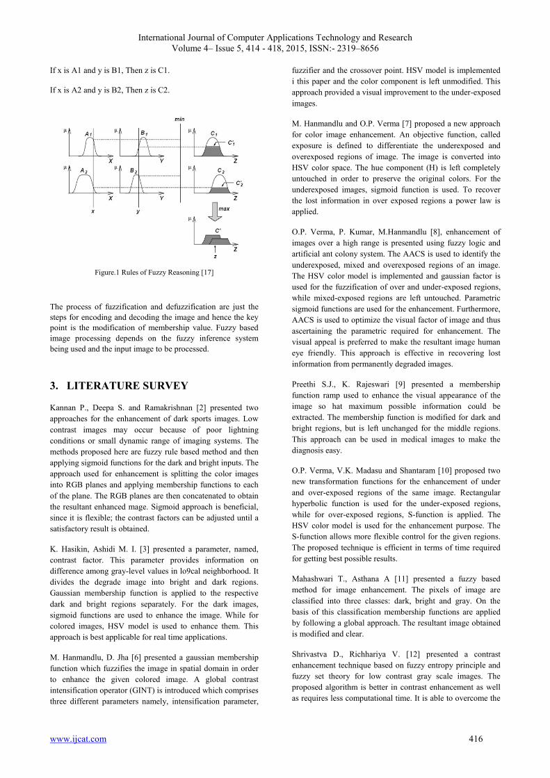
International Journal of Computer Applications Technology and Research
Volume 4– Issue 5, 414 - 418, 2015, ISSN:- 2319–8656
www.ijcat.com 416
If x is A1 and y is B1, Then z is C1.
If x is A2 and y is B2, Then z is C2.
Figure.1 Rules of Fuzzy Reasoning [17]
The process of fuzzification and defuzzification are just the
steps for encoding and decoding the image and hence the key
point is the modification of membership value. Fuzzy based
image processing depends on the fuzzy inference system
being used and the input image to be processed.
3. LITERATURE SURVEY
Kannan P., Deepa S. and Ramakrishnan [2] presented two
approaches for the enhancement of dark sports images. Low
contrast images may occur because of poor lightning
conditions or small dynamic range of imaging systems. The
methods proposed here are fuzzy rule based method and then
applying sigmoid functions for the dark and bright inputs. The
approach used for enhancement is splitting the color images
into RGB planes and applying membership functions to each
of the plane. The RGB planes are then concatenated to obtain
the resultant enhanced mage. Sigmoid approach is beneficial,
since it is flexible; the contrast factors can be adjusted until a
satisfactory result is obtained.
K. Hasikin, Ashidi M. I. [3] presented a parameter, named,
contrast factor. This parameter provides information on
difference among gray-level values in lo9cal neighborhood. It
divides the degrade image into bright and dark regions.
Gaussian membership function is applied to the respective
dark and bright regions separately. For the dark images,
sigmoid functions are used to enhance the image. While for
colored images, HSV model is used to enhance them. This
approach is best applicable for real time applications.
M. Hanmandlu, D. Jha [6] presented a gaussian membership
function which fuzzifies the image in spatial domain in order
to enhance the given colored image. A global contrast
intensification operator (GINT) is introduced which comprises
three different parameters namely, intensification parameter,
fuzzifier and the crossover point. HSV model is implemented
i this paper and the color component is left unmodified. This
approach provided a visual improvement to the under-exposed
images.
M. Hanmandlu and O.P. Verma [7] proposed a new approach
for color image enhancement. An objective function, called
exposure is defined to differentiate the underexposed and
overexposed regions of image. The image is converted into
HSV color space. The hue component (H) is left completely
untouched in order to preserve the original colors. For the
underexposed images, sigmoid function is used. To recover
the lost information in over exposed regions a power law is
applied.
O.P. Verma, P. Kumar, M.Hanmandlu [8], enhancement of
images over a high range is presented using fuzzy logic and
artificial ant colony system. The AACS is used to identify the
underexposed, mixed and overexposed regions of an image.
The HSV color model is implemented and gaussian factor is
used for the fuzzification of over and under-exposed regions,
while mixed-exposed regions are left untouched. Parametric
sigmoid functions are used for the enhancement. Furthermore,
AACS is used to optimize the visual factor of image and thus
ascertaining the parametric required for enhancement. The
visual appeal is preferred to make the resultant image human
eye friendly. This approach is effective in recovering lost
information from permanently degraded images.
Preethi S.J., K. Rajeswari [9] presented a membership
function ramp used to enhance the visual appearance of the
image so hat maximum possible information could be
extracted. The membership function is modified for dark and
bright regions, but is left unchanged for the middle regions.
This approach can be used in medical images to make the
diagnosis easy.
O.P. Verma, V.K. Madasu and Shantaram [10] proposed two
new transformation functions for the enhancement of under
and over-exposed regions of the same image. Rectangular
hyperbolic function is used for the under-exposed regions,
while for over-exposed regions, S-function is applied. The
HSV color model is used for the enhancement purpose. The
S-function allows more flexible control for the given regions.
The proposed technique is efficient in terms of time required
for getting best possible results.
Mahashwari T., Asthana A [11] presented a fuzzy based
method for image enhancement. The pixels of image are
classified into three classes: dark, bright and gray. On the
basis of this classification membership functions are applied
by following a global approach. The resultant image obtained
is modified and clear.
Shrivastva D., Richhariya V. [12] presented a contrast
enhancement technique based on fuzzy entropy principle and
fuzzy set theory for low contrast gray scale images. The
proposed algorithm is better in contrast enhancement as well
as requires less computational time. It is able to overcome the

International Journal of Computer Applications Technology and Research
Volume 4– Issue 5, 414 - 418, 2015, ISSN:- 2319–8656
www.ijcat.com 417
drawbacks of spatial domain methods of thresholding. It
results in high contrast images.
Chamorro J., Sanchez D. [13] discussed various cardinalities
of fuzzy sets and their uses in quantification. The study shows
that scalar measures are not well suited for measuring
cardinalities and fuzzy numbers suit this well. A new fuzzy
based method has been proposed to evaluate the quantified
sentences. Linguistic histograms have resulted in more
appropriate approach to provide inputs to users. The concepts
of color have been defined very well using fuzzy based
approach which can be efficiently used in fuzzy image
processing.
Raju G. and Madhu S. Nair [14] presented a fast and efficient
fuzzy based color image enhancement method for enhancing
low contrast color images. This method is based on two
parameters M and K, where M is average intensity value of
image and K is contrast intensification parameter. The image's
RGB factor is converted into HSV color space. To enhance
the image, V factor i.e. intensity is stretched under the control
of M and K. The basic principle on which the technique is
designed is transforming skewed histogram of input image
into a uniform histogram. The proposed algorithm is
compared with conventional techniques. Beside the visual
results and computational time, Contrast Improvement Index
(CII) and Tenengrad measure are two quantitative measures
used for performance analysis. The tenengrad value is larger
for high quality images which show that it enhances the
structural information, and thus is the result obtained after
applying this approach to images. The proposed method is
computationally faster than the existing methods and well
suits with the images having background with non-uniform
distribution of brightness.
Chi-FarnChen , Hung-Yu Chang, Li-Yu Chang [15] presented
fuzzy-based approach to enhance the contrast and brightness
information on the image. The test results indicated that the
proposed method provides better contrast image compared to
the conventional enhancement methods in terms of visibility
and image details. Two image quality indices have been used
to evaluate the performance of the proposed enhancement
technique. The comparison of proposed technique with
conventional enhancement techniques showed that the
proposed method can produce better measurements compared
to the conventional techniques. The stretch method used to
enhance each cluster is generated by way of a linear model
with stretch parameters.
4. GAPS IN LITERATURE:
The existing contrast intensification parameter (K), has been
taken 128 by most of the researchers, which is only feasible
for very low contrast images' enhancement and hence over-
contrast images when enhanced result in loss of information.
The traditional methods even lay no attention to the regions or
objects present in image and enhancement is performed by
predefined rules thus resulting in color imbalance of the
output image. Conventional techniques also result in images
with degraded edges. Since, edges play a significant role in
extracting information from images, proposed technique will
concentrate on edge restoration as well.
5. Conclusion:
This paper has presented a study on various image
enhancement techniques. The review has shown that there are
still many improvements required in the available techniques
to handle different kind of images. This paper has shown that
no particular technique is effective for every kind of images or
image data set. Although fuzzy logic and histogram based
techniques have shown quite significant results but it still face
many issues. To overcome the limitations of existing
techniques a new technique will be proposed in near future
which will evaluate K factor of fuzzy based enhancement
automatically using the ant colony optimization to find the
best similarity value among the given set of values which
represents the image in more efficient manner.
6. REFERENCES:
[1] Gonzalez RC, Woods RE. 2002. Digital image processing.
2nd ed. Englewood Cliffs, NJ: Prentice-Hall. ISBN: 0-201-
18075-8.
[2] Kannan, P., S. Deepa, and R. Ramakrishnan. 2012.
"Contrast enhancement of sports images using two
comparative approaches." American Journal of Intelligent
Systems 2.6: 141-147.
[3] Hasikin, Khairunnisa, and NorAshidi Mat Isa. 2013.
"Adaptive fuzzy intensity measure enhancement technique for
non-uniform illumination and low-contrast images." Signal,
Image and Video Processing: 1-24.
[4] Kim, Yeong-Taeg. 1997. "Contrast enhancement using
brightness preserving bi-histogram equalization." Consumer
Electronics, IEEE Transactions on 43.1: 1-8.
[5] Arici, Tarik, SalihDikbas, and YucelAltunbasak. 2009. "A
histogram modification framework and its application for
image contrast enhancement." Image processing, IEEE
Transactions on 18.9: 1921-1935.
[6] Hanmandlu, Madasu, and DevendraJha. 2006. "An
optimal fuzzy system for color image enhancement." Image
Processing, IEEE Transactions on 15.10 : 2956-2966.

International Journal of Computer Applications Technology and Research
Volume 4– Issue 5, 414 - 418, 2015, ISSN:- 2319–8656
www.ijcat.com 418
[7] Hanmandlu, Madasu, et al. 2009. "A novel optimal fuzzy
system for color image enhancement using bacterial
foraging." Instrumentation and Measurement, IEEE
Transactions on 58.8 : 2867-2879.
[8] Verma, Om Prakash, et al. 2012. "High dynamic range
optimal fuzzy color image enhancement using artificial ant
colony system." Applied Soft Computing 12.1 : 394-404.
[9] SJ, MrsPreethi, and Mrs K. Rajeswari. "Membership
Function modification for Image Enhancement using fuzzy
logic."
[10] Verma, Om Prakash, V. K. Madasu, and V. Shantaram.
2011. "High Dynamic Range Color Image Enhancement
Using Fuzzy Logic and Bacterial Foraging." Defence Science
Journal 61.5 : 462-472.
[11] Mahashwari, Tarun, and Amit Asthana. 2013. "Image
enhancement using fuzzy technique." International Journal of
Research in Engineering Science and Technology 2.2 : 1-4.
[12] Shrivastava, Diwakar, and VineetRichhariya, "Analytical
Survey on various parameters."
[13] Chamorro-Martínez, J., et al. 2014. "A discussion on
fuzzy cardinality and quantification. Some applications in
image processing." Fuzzy Sets and Systems 257 : 85-101.
[14] Raju G., and Madhu S. Nair. 2014. "A fast and efficient
color image enhancement method based on fuzzy-logic and
histogram." AEU-International Journal of Electronics and
Communications 68.3 : 237-243.
[15] Chen, Chi-Farn, Hung-Yu Chang, and Li-Yu Chang.
2008. "A Fuzzy-based method for remote sensing image
contrast enhancement." The International Archives of the
Photogrammetry, Remote Sensing and Spatial Information
Sciences 37 :995-998.
[16] Zadeh, Lotfi A. 1975. "The concept of a linguistic
variable and its application to approximate reasoning—II."
Information sciences 8.4 : 301-357.
[17] Tizhoosh 1997. "Contrast Improvement based on Fuzzy
If-Then rules.
[18] Tizhoosh, Hamid R. 1997. "Fuzzy image processing."
Publisher: Springer-Verlag. Kartoniert (TB), Deutsch.
Related Documents