Heterogeneous Responses to Effective Tax Enforcement: Evidence from Spanish Firms

Heterogeneous Responses to Effective Tax

Enforcement: Evidence from Spanish Firms∗

Miguel Almunia David Lopez-Rodriguez

University of Warwick Banco de España

July 18, 2014

Abstract

We investigate whether monitoring the information trails generated by firms’ ac-tivities improves tax compliance. We exploit quasi-experimental variation generatedby a Large Taxpayers’ Unit (LTU) in Spain, which devotes additional resources toverifying the transactions reported by firms with more than e6 million in reportedrevenue. Firms bunch below this threshold in order to avoid stricter tax enforce-ment, and this reaction is stronger in sectors where paper trail is easier to monitor.These results suggest that monitoring efforts by the tax authority and the trace-ability of information reported by firms are complements, and both are necessaryfor effective tax enforcement.

Keywords: tax enforcement, firms, bunching, Spain, Large Taxpayers Unit (LTU).

JEL codes: H26, H32.

∗Almunia (corresponding author): [email protected], University of Warwick Department ofEconomics and Centre for Competitive Advantage in the Global Economy (CAGE). Lopez-Rodriguez:[email protected], Banco de España. We thank Emmanuel Saez, Alan Auerbach, Fred Finan and TedMiguel for constant support and encouragement throughout this project. We gratefully acknowledgemany useful comments and suggestions from Juan Pablo Atal, Henrique Basso, Michael Best, David Card,Lorenzo Casaburi, Raj Chetty, Francisco de la Torre, François Gerard, Jonas Hjort, Simon Jäger, AttilaLindner, Justin McCrary, Craig McIntosh, Adair Morse, Gautam Rao, Ana Rocca, Michel Serafinelli,Monica Singhal, Juan Carlos Suárez Serrato, Victoria Vanasco, Andrea Weber, Danny Yagan, Owen Zidarand numerous seminar participants. Almunia gratefully acknowledges financial support from FundaciónRafael del Pino and the Burch Center for Tax Policy and Public Finance. Any views expressed in thispaper are only those of the authors and should not be attributed to the Banco de España.

1 Introduction

Modern tax systems in advanced economies feature high levels of tax compliance despite

low audit rates, an outcome at odds with the predictions of the classical deterrence model

of tax evasion (Allingham and Sandmo, 1972). More recent theoretical studies argue

that third-party information reporting is critical to reconcile these two facts because

of its additional deterrence effect on taxpayers (Kopczuk and Slemrod, 2006; Kleven,

Kreiner and Saez, 2009; Gordon and Li, 2009). Indeed, experimental evidence shows

that individual income tax compliance is much higher when the tax authority has the

capacity to match tax returns and third-party information reports in a systematic way

(Slemrod, Blumenthal and Christian, 2001; Kleven et al., 2011). Even though firms

produce the majority of these reports and they remit1 most of the tax payments collected

by governments, empirical studies of tax compliance usually focus on individuals, rather

than analyzing firm behavior.

This paper contributes to fill this gap by analyzing whether the existence of third-

party reporting is sufficient to ensure high tax compliance by firms. First, we derive

theoretical predictions on how firms respond to higher tax enforcement intensity, which

results from the more effective use of the information trails created by firms’ activities

through various channels. These predictions are then tested using quasi-experimental

variation provided by the Large Taxpayers Unit (LTU) in Spain.2 The Spanish LTU, a

special unit within the tax authority, devotes additional monetary and human resources

to verify tax returns (e.g., audits) and monitor activities of firms with more than e6

million in annual operating revenue. The monitoring intensity changes discretely at

this arbitrary revenue threshold, while firms just below and above face the same tax

schedule and information requirements. This allows us to study the effect of stricter tax

enforcement on firms’ compliance behavior.

In our baseline theoretical framework, firms with heterogeneous productivities make

their production and tax reporting decisions to maximize expected profits, for a given tax

rate on reported profits. There is an incentive to misreport revenue because it lowers tax

liability, but to do so firms incur some resource costs (e.g., keeping two sets of accounting

books or foregoing business opportunities). The deterrence component of tax compli-

ance is captured by a detection probability that increases endogenously with the amount

1For instance, in the United States firms remit 84% of all taxes collected by the federal government(Christensen, Cline and Neubig, 2001). As taxpayers, they remit corporate income tax and a share ofpayroll tax. As tax collectors, they withhold income and payroll tax from employees. In other advancedcountries, firms also remit value added tax (VAT) payments.

2Many tax authorities in advanced countries, and an increasing number of emerging countries, havesome type of LTU to deal with large businesses (IMF, 2002; OECD, 2011). Firms in the Spanish LTUrepresent 2.5% of all registered businesses, employ 40% of private sector workers and report 80% oftaxable profits (AEAT, 1999-2008).

1

evaded by firms. This probability results from the interaction between (i) the resources

devoted by the tax authority to monitor firms (“monitoring effort”); and (ii) the existing

enforcement technology to analyze tax returns and systematically check them against

other information generated by business transactions. We introduce a notch in tax en-

forcement intensity by assuming that monitoring effort jumps up discretely at a fixed

level of reported revenue, while reporting requirements and the enforcement technology

remain constant. The increase in monitoring resources above the threshold strengthens

the effectiveness of the enforcement technology, leading firms to bunch below the LTU

threshold in order to avoid more effective tax enforcement. Absent prohibitive resource

costs, the bunching response creates a “hole” in the distribution of reported revenue with

zero mass in an interval above the tax enforcement notch. We discuss below an extended

model where resource costs of evasion may prevent the reaction to the threshold.

In the empirical analysis, we use financial statements and balance-sheet data reported

by Spanish firms to the Commercial Registry. This dataset, compiled at the European

level by Amadeus, contains firm-level information on annual operating revenue, input

expenditures, fixed assets and number of employees, making it possible to analyze multiple

margins of firms’ responses to the tax enforcement threshold. In addition, the longitudinal

structure of the dataset allows us to analyze the dynamic behavior of firms. The dataset

covers more than 80% of registered businesses in Spain with operating revenue in the

e3-e9 million range for the period 1999-2007, during which the LTU threshold remained

constant at e6 million.

The first set of results shows a considerable reaction to avoid the stricter monitor-

ing effort by the tax agency. Consistent with the predicted response to more effective

tax enforcement, we find substantial bunching of firms just below the LTU threshold in

the empirical distribution of reported revenue. Adopting the empirical procedure devel-

oped in Kleven and Waseem (2013), we quantify the effect of larger tax enforcement on

firms’ reported revenue by comparing the observed and the counterfactual revenue den-

sity around the threshold. Estimates indicate that, on average, bunching firms reduce

their reported revenue by e101,000 (about 1.7% of total revenue) to stay under lower

monitoring effort. Considering that high resource costs of evasion prevent some firms

from responding, the adjusted estimates show that the marginal bunching firm reduces

reported revenue by about e593,000 (almost 10% of total revenue). Both estimates are

statistically significant at the 1% level. Robustness checks indicate that the bunching

response is neither due to other size-contingent regulations nor caused by the persistence

of a small group of firms just below the threshold. Moreover, the estimates are robust to

different assumptions when estimating the counterfactual distribution.

The second set of results illustrates the role of deterrence and resource costs on the tax

2

compliance behavior of firms. We extend the baseline model along two dimensions to allow

for heterogeneous responses across different firm characteristics: the traceability of firms’

transactions and the resource costs related to evasion. In the first extension, we consider

how the position in the production chain affects the traceability of a firm’s transactions.

When a firm sells intermediate inputs, transactions generate substantial information trails

so it is easier for the tax agency to detect evasion by matching tax returns to other

information sources. In contrast, sales to final consumers tend to leave little or no paper

trail, so even an exhaustive audit by the LTU may be unable to detect evasion. Hence,

variation in the traceability of transactions implies that the same monitoring effort results

in different effective enforcement intensities for each firm, holding revenue fixed. We

test this hypothesis empirically dividing the data into ten sectors of activity. We find

that the bunching response is strongest in sectors that sell mostly intermediate inputs

(e.g., wholesalers, heavy manufacturers) and much weaker in sectors that sell mostly

to final consumers (e.g., retailers, restaurants and hotels). This result indicates that

the effectiveness of additional monitoring effort depends crucially on the traceability of

firms’ transactions. In terms of our theoretical framework, this finding suggests that

information reporting requirements and monitoring resources are complements, because

it is the interaction between the two that deters firms from evading taxes.

In the second extension, we allow for variation in the resource costs of evasion. These

costs reduce the profitability of tax evasion and hence lower the incentives to misreport

revenue (regardless of monitoring effort). In some cases, resource costs may be so high

that firms do not misreport their revenue at all. This could be due to the complexity of

firms’ operations, which makes tax evasion unfeasible because it is too costly compared to

the expected benefits (Kleven, Kreiner and Saez, 2009). The presence of such prohibitive

resource costs of evasion for a significant proportion of firms not only attenuates the

bunching response, but it also helps explain why we observe only a small dip, rather than

a hole, in the distribution of revenue just above the LTU threshold. To complement this

analysis, we divide the sample using proxies for the complexity of firms’ operations. We

find that bunching is lower, but still significant, among firms with more employees and a

larger stock of fixed assets, confirming the intuition that complexity of operations affects

the relevance of resource costs.

The third set of results analyzes the mechanisms behind firms’ responses to avoid more

effective tax enforcement. To do this, we consider a model in which firms may also mis-

report their input expenditures. Firms have incentives to overreport their materials (to

lower their VAT and corporate income tax liabilities) and underreport labor expenditures

(to lower their payroll tax liabilities).3 The model’s predictions depend on whether the

3Underreporting labor expenditures increases corporate tax liabilities, but this can be compensated

3

bunching response is due to real (i.e. lower output) or evasion (i.e. increase of concealed

revenue) adjustments. We assess the plausibility of each type of response using a sim-

ple graphical test where the outcomes are the reported ratios of input expenditures over

revenue. We find that the average ratio of material expenditures for firms just below the

LTU threshold is 66%, but the ratio shifts down to 64% for firms just above. In contrast,

average labor expenditures shift up from 15% below threshold to 16% above. According

to our theoretical predictions, these empirical patterns are not compatible with a real

response, which would have resulted in upward shifts of both inputs at the threshold (be-

cause bunching firms are more productive). Instead, the evidence is fully consistent with

an evasion response in which bunching firms strategically misreport their expenditures to

maximize tax evasion.4 While we cannot infer causality from these patterns, they provide

suggestive evidence that firms are able to misreport their input expenditures when they

are under low monitoring effort, even in the presence of third-party reporting.

The findings in this paper contribute to the thin empirical literature on business tax

evasion by providing a well-identified measure of the effects of tax enforcement on firm

behavior in an advanced economy. De Paula and Scheinkman (2010) and Pomeranz

(2013) emphasize the key role of information for effective tax enforcement, particularly

through the self-enforcing mechanisms of the VAT.5 In an experiment with small Chilean

firms, Pomeranz (2013) finds that the VAT paper trail acts as a substitute of tax audits

to improve tax compliance. In contrast, our results suggest that additional resources to

perform audits and the existence of information trails are complements and that both are

necessary to increase tax compliance by firms. Showing another limitation of third-party

reporting, Carrillo, Singhal and Pomeranz (2014) find that firms in Ecuador respond

to the use of third-party reported information by substituting evasion into less verifi-

able margins, such as input expenditures. We also contribute by providing evidence on

the importance of resource costs of evasion, related with firms’ size and complexity (as

discussed in Kleven, Kreiner and Saez, 2009).

The empirical techniques used in this paper draw on a growing literature in pub-

lic finance that analyzes agents’ responses to thresholds in taxes and regulations. In

the seminal paper of this literature, Saez (2010) exploits kinks—i.e., income thresholds

by the tax savings on the payroll tax. During the period under study, the statutory payroll tax in Spainwas 38% (including both the employer’s and the employee’s shares), compared to a corporate income taxrate that declined from 35% to 30%. Moreover, keeping reported salaries low and paying part under thetable protects firms against future negative shocks, because there is downward nominal wage rigidity.

4Disaggregating labor expenditures, we find evidence on wage misreporting with a downward jumpof average wages for firms just below the threshold, while the average number of employees is similararound it. There is additional theoretical support for labor misreporting in Yaniv (1988), and pervasiveevidence of salary underreporting in many countries, as shown in recent empirical studies such as Kumler,Verhoogen and Frias (2012) and Best (2013), and even in the US (Slemrod and Gillitzer, 2014).

5In fiscal systems with a VAT, the transmission of evasion (or compliance) behavior moves upwardsthe production chain from retailers to intermediate goods suppliers.

4

at which the marginal tax rate jumps—to identify taxable income elasticities.6 Our

estimation strategy is most closely-related to Kleven and Waseem (2013), who exploit

notches—income thresholds at which the average tax rate jumps.7 The novel feature of

our setting is that the Spanish LTU generates a notch in enforcement intensity, rather

than the tax rate, allowing us to study the effects of tax enforcement policies in isolation.

Finally, our paper contributes to an extensive literature on the effects of size-dependent

policies and regulations on firm behavior. One strand of this literature has focused on

the impact of such regulations on productivity, given the pervasive incentives for firms

to remain inefficiently small (Guner, Ventura and Xu, 2008; Restuccia and Rogerson,

2008; Garicano, LeLarge and van Reenen, 2013). Other studies have instead focused on

evasion and avoidance responses. For instance, Onji (2009) shows that Japanese firms

reacted to the introduction of a VAT eligibility threshold by splitting into several smaller

entities in other to avoid taxation. In a similar vein, our results show that some firms

may look smaller in the data than they are in reality because of misreporting under low

tax enforcement, which could have important implications for productivity estimations

in many contexts.

The rest of the paper is organized as follows. Section 2 presents the theoretical frame-

work. Section 3 describes the empirical strategy and derives the bunching estimators.

Section 4 provides institutional context and describes the data. Section 5 presents the

estimation results. Section 6 concludes.

2 Theoretical Framework

We model the problem of profit-maximizing firms that can evade taxes and face the risk

of being detected (and punished) by the tax authority. In the basic setting, firms make

production decisions and are able to misreport their revenue, but they bear resource

costs associated to tax evasion. The probability of detection depends on the tax author-

ity’s monitoring efforts and the available technology to cross-check tax returns to find

inconsistencies in reporting, taking advantage of the paper trail generated by information

requirements. This probability therefore depends endogenously on each firm’s level of

evasion. We use this framework to examine how firms respond to a discontinuity in tax

enforcement intensity generated by a sharp increase in monitoring efforts at an arbitrary

6A number of recent studies apply Saez’s method to derive taxable income elasticities using largeadministrative datasets from Denmark, Sweden and the United States (Chetty et al., 2011; Bastani andSelin, 2014; Chetty, Friedman and Saez, 2013). Devereux, Liu and Loretz (2014) also use bunchingtechniques to estimate the elasticity of corporate taxable income in the United Kingdom.

7Slemrod (2010) provides a general description of notches in tax and regulatory systems. Two recentworking papers, Best and Kleven (2013) and Kopczuk and Munroe (forthcoming) study notches generatedby property transaction taxes.

5

revenue threshold. We then extend the model to allow for heterogeneity across firms

in the resource costs of evasion and in the effective monitoring intensity, which yields

testable predictions about the shape of the distribution of reported revenue.

2.1 Corporate Taxation with Risky Evasion

Consider an economy with a continuum of firms of measure one whose income is taxed

by the government. Firms produce good y combining tax-deductible inputs x and nond-

eductible inputs z according to the production function y = ψf(x, z), where ψ is a pro-

ductivity parameter and f(·, ·) is strictly continuous, increasing and concave in both ar-

guments. Productivity ψ is exogenously distributed over the range [ψ,ψ] with a smoothly

decreasing and convex density d0(ψ) in the population of firms. Firms purchase deductible

and nondeductible inputs in competitive markets at unit cost w and q, respectively, and

sell their output at the market price p, which is normalized to unity.

The government levies a proportional tax t on taxable profits P = y − wx, so net-of-

tax profits with truthful reporting are given by Π = (1−t)P−qz. Since the tax authority

does not perfectly observe all transactions in the economy, firms may attempt to evade

taxes by misreporting taxable profits. In the baseline case, firms can underreport their

revenue by an amount u ≡ y−y ≥ 0, where y is reported revenue8 and, therefore, reported

taxable profits are given by P = (1 − t)[y − wx]. The direct and indirect resource costs

of evasion are captured with the reduced form κ(u), which is an increasing and convex

function of concealed revenue.9

The tax authority detects evasion with probability δ = φh(u), where φ > 0 is an en-

forcement intensity parameter, and h(·) is a continuous, increasing and convex function

in concealed revenue. Enforcement intensity φ measures the monitoring effort exerted by

the tax authority, which depends on the resources devoted toe examine firms’ tax returns

and undertake tax audits. The endogenous component, h(u), represents the technology

used to match tax returns among trading partners and to review the paper trail created

by information-reporting requirements. This component captures the intuition that a

larger amount of unreported sales increases the probability of detection because each

inconsistency in reported transactions leaves a paper trail that can be examined (e.g.

discrepancies in the monetary value of sales reported by firms and the purchases claimed

as tax credits by their clients). Hence, the detection probability is determined by the

8In subsection 5.4, we discuss the predictions of an extended model in which firms can also evadetaxes by misreporting their input costs. We fully derive the extended model in the online appendix.

9One example of these resource costs of evasion is the need to maintain parallel accounting books tokeep track of black payments in cash. Tax evading firms may also forego business opportunities by notaccepting credit cards or bank payments, given that it is much easier to conceal cash transactions. SeeChetty (2009) for a detailed discussion on the economic nature of these resource costs.

6

interaction between the resources devoted to monitoring φ and the enforcement technol-

ogy h (u). Intuitively, these two elements are complementary and both are necessary to

achieve effective tax enforcement. For simplicity, we assume that when discrepancies be-

tween firms’ reported transactions are detected, the authorities uncover the full amount

evaded. Whenever evasion is detected, the tax authority imposes a fine with a penalty

rate θ over the amount of tax evaded, on top of the true tax liability.10

Firms make production (i.e., demand of inputs x and z) and reporting (i.e., underre-

ported revenue u) decisions in order to maximize expected after-tax profit, given by

EΠ = (1− t)[ψf(x, z)− wx]− qz − κ(u) + tu[1− φh(u)(1 + θ)]. (1)

An interior optimum satisfies the following system of first-order conditions:11

ψfx(x, z) = w (2)

ψfz(x, z) = q/(1− t) (3)

t[1− φh(u)(1 + θ)] = κu(u) + tu(1 + θ)φhu(u) (4)

where the term [1 − φh(u)(1 + θ)] ≡ r is the expected rate of return of evasion. This

system of equations indicates that a positive tax rate has two effects. First, it distorts

the choice of inputs, reducing production below the zero-tax optimum. Second, it creates

incentives to evade taxes, thereby reducing reported revenue for all firms in equilibrium.

Simple comparative statics show that an increase in enforcement intensity φ leads to a

decrease in concealed revenue u.

To provide more intuition on firms’ incentives to evade taxes, we define the elasticity

of detection probability with respect to concealed income as εδ,u ≡ φhu · u/δ, and rewrite

the optimal evasion condition (4) as follows12

1 =κu(u)

t+ (1 + θ)δ(u) [1 + εδ,u] . (5)

The right-hand side of (5) identifies the two mechanisms that contribute to raising tax

compliance by firms. The first term shows the disincentive effect created by the presence

of marginal resource costs (relative to the marginal benefit of evasion, i.e., the tax rate).

The second term represents the deterrence effect generated by the interaction between

10The canonical Allingham and Sandmo (1972) model of income tax evasion assumes that the penaltyapplies to the total amount evaded, but Yitzhaki (1974) points out that the common practice in mostcountries is to make the penalty proportional to the amount of tax evaded.

11The assumption of convex detection probability is sufficient to ensure the second-order condition forinterior optimum is satisfied.

12This equation is similar to the one derived by Kleven et al. (2011), but obtained from the choiceproblem of firms, with an additional term to capture the impact of resource costs of evasion.

7

the tax authority’s monitoring effort and the existence of a paper trail generated by

misreporting behavior.

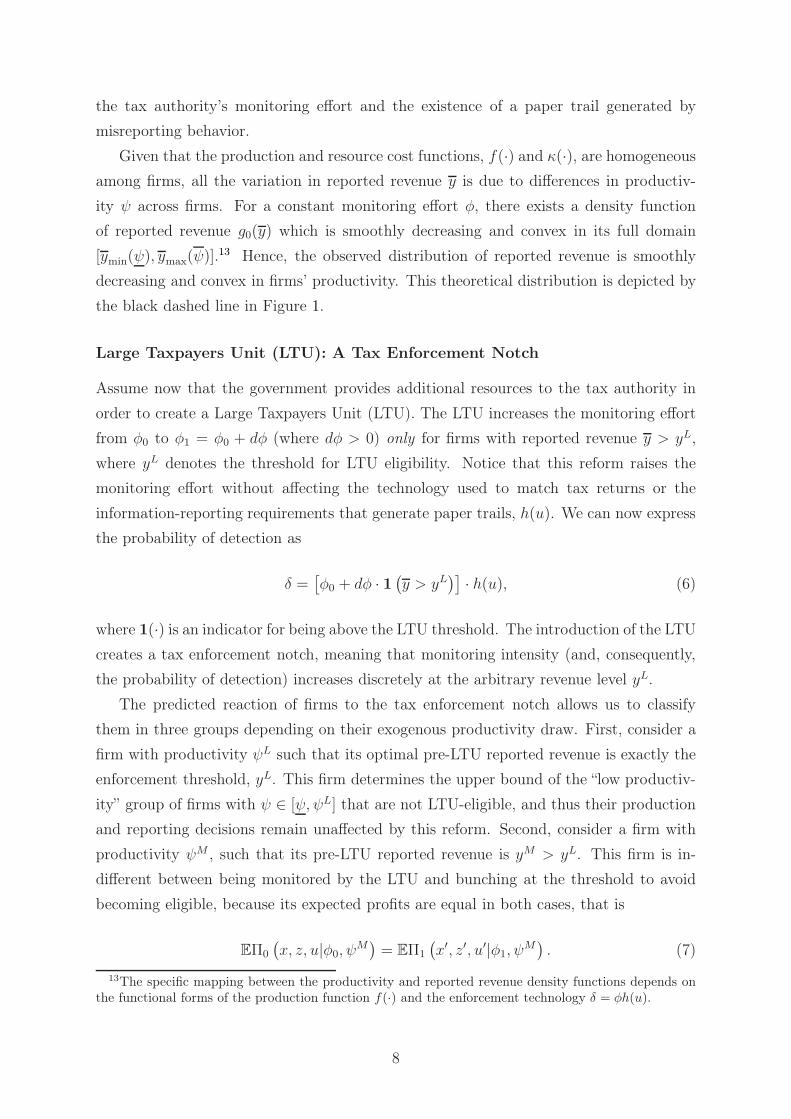
Given that the production and resource cost functions, f(·) and κ(·), are homogeneous

among firms, all the variation in reported revenue y is due to differences in productiv-

ity ψ across firms. For a constant monitoring effort φ, there exists a density function

of reported revenue g0(y) which is smoothly decreasing and convex in its full domain

[ymin(ψ), ymax(ψ)].13 Hence, the observed distribution of reported revenue is smoothly

decreasing and convex in firms’ productivity. This theoretical distribution is depicted by

the black dashed line in Figure 1.

Large Taxpayers Unit (LTU): A Tax Enforcement Notch

Assume now that the government provides additional resources to the tax authority in

order to create a Large Taxpayers Unit (LTU). The LTU increases the monitoring effort

from φ0 to φ1 = φ0 + dφ (where dφ > 0) only for firms with reported revenue y > yL,

where yL denotes the threshold for LTU eligibility. Notice that this reform raises the

monitoring effort without affecting the technology used to match tax returns or the

information-reporting requirements that generate paper trails, h(u). We can now express

the probability of detection as

δ =!φ0 + dφ · 1

"y > yL

#$· h(u), (6)

where 1(·) is an indicator for being above the LTU threshold. The introduction of the LTU

creates a tax enforcement notch, meaning that monitoring intensity (and, consequently,

the probability of detection) increases discretely at the arbitrary revenue level yL.

The predicted reaction of firms to the tax enforcement notch allows us to classify

them in three groups depending on their exogenous productivity draw. First, consider a

firm with productivity ψL such that its optimal pre-LTU reported revenue is exactly the

enforcement threshold, yL. This firm determines the upper bound of the “low productiv-

ity” group of firms with ψ ∈ [ψ,ψL] that are not LTU-eligible, and thus their production

and reporting decisions remain unaffected by this reform. Second, consider a firm with

productivity ψM , such that its pre-LTU reported revenue is yM > yL. This firm is in-

different between being monitored by the LTU and bunching at the threshold to avoid

becoming eligible, because its expected profits are equal in both cases, that is

EΠ0

"x, z, u|φ0,ψ

M#= EΠ1

"x′, z′, u′|φ1,ψ

M#. (7)

13The specific mapping between the productivity and reported revenue density functions depends onthe functional forms of the production function f(·) and the enforcement technology δ = φh(u).

8

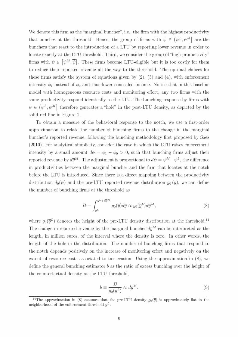
We denote this firm as the “marginal buncher”, i.e., the firm with the highest productivity

that bunches at the threshold. Hence, the group of firms with ψ ∈"ψL,ψM

$are the

bunchers that react to the introduction of a LTU by reporting lower revenue in order to

locate exactly at the LTU threshold. Third, we consider the group of “high productivity”

firms with ψ ∈!ψM ,ψ

$. These firms become LTU-eligible but it is too costly for them

to reduce their reported revenue all the way to the threshold. The optimal choices for

these firms satisfy the system of equations given by (2), (3) and (4), with enforcement

intensity φ1 instead of φ0 and thus lower concealed income. Notice that in this baseline

model with homogeneous resource costs and monitoring effort, any two firms with the

same productivity respond identically to the LTU. The bunching response by firms with

ψ ∈"ψL,ψM

$therefore generates a “hole” in the post-LTU density, as depicted by the

solid red line in Figure 1.

To obtain a measure of the behavioral response to the notch, we use a first-order

approximation to relate the number of bunching firms to the change in the marginal

buncher’s reported revenue, following the bunching methodology first proposed by Saez

(2010). For analytical simplicity, consider the case in which the LTU raises enforcement

intensity by a small amount dφ = φ1 − φ0 > 0, such that bunching firms adjust their

reported revenue by dyM . The adjustment is proportional to dψ = ψM−ψL, the difference

in productivities between the marginal buncher and the firm that locates at the notch

before the LTU is introduced. Since there is a direct mapping between the productivity

distribution d0(ψ) and the pre-LTU reported revenue distribution g0 (y), we can define

the number of bunching firms at the threshold as

B =

ˆ yL+dyM

yLg0(y)dy ≈ g0(y

L)dyM , (8)

where g0(yL) denotes the height of the pre-LTU density distribution at the threshold.14

The change in reported revenue by the marginal buncher dyM can be interpreted as the

length, in million euros, of the interval where the density is zero. In other words, the

length of the hole in the distribution. The number of bunching firms that respond to

the notch depends positively on the increase of monitoring effort and negatively on the

extent of resource costs associated to tax evasion. Using the approximation in (8), we

define the general bunching estimator b as the ratio of excess bunching over the height of

the counterfactual density at the LTU threshold,

b ≡B

g0(yL)≈ dyM . (9)

14The approximation in (8) assumes that the pre-LTU density g0(y) is approximately flat in theneighborhood of the enforcement threshold yL.

9

2.2 Heterogeneous Firms

In the baseline model outlined above, we assume that (i) a discrete jump in monitoring

intensity translates into the same change in enforcement intensity for all firms above the

LTU threshold, and (ii) all taxpayers face the same resource costs of evasion. Given these

simplifying assumptions, the model predicts bunching at the LTU threshold (with zero

mass of firms in an interval just above it), and that all the variation in firms’ reported

revenue is due to differences in productivity. We now extend the model to introduce

heterogeneity across firms in both enforcement intensity and resource costs. We show

how this heterogeneity leads to different incentives to bunch for firms with the same

productivity level. As a consequence, the extended model no longer predicts a hole in the

post-LTU revenue distribution, and allows us to disentangle firms’ structural response to

effective tax enforcement from the average response attenuated by the presence of high

resource costs.

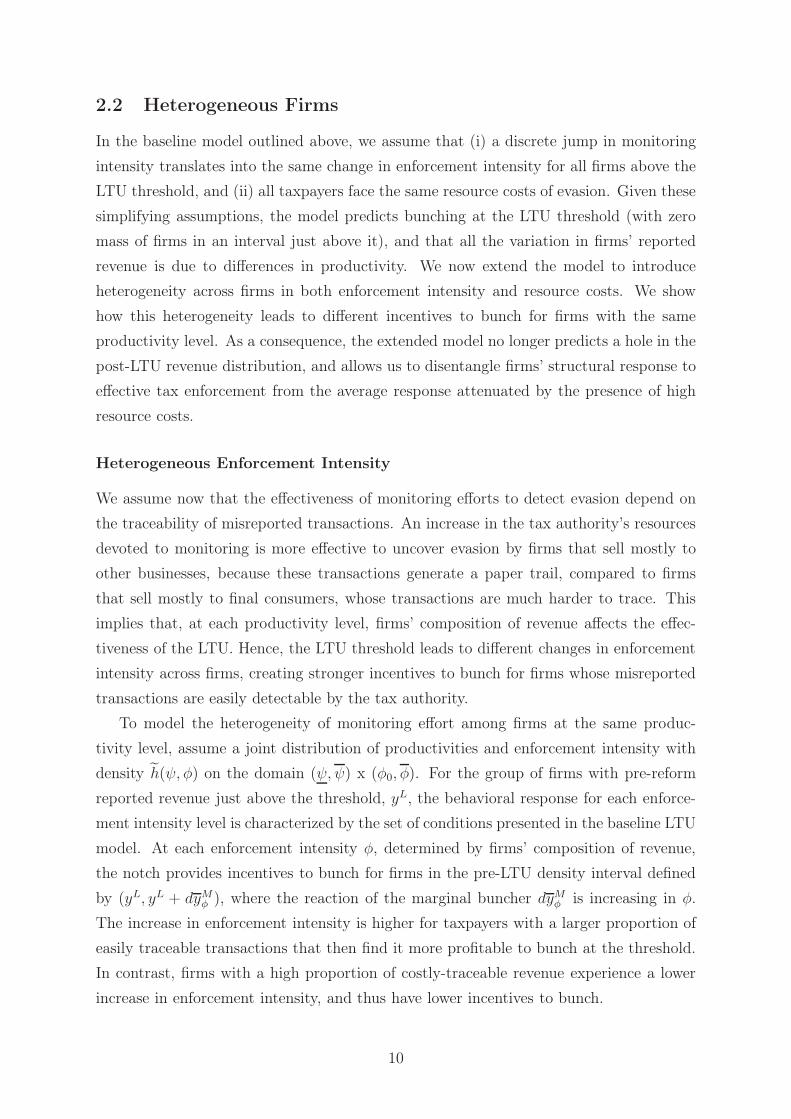
Heterogeneous Enforcement Intensity

We assume now that the effectiveness of monitoring efforts to detect evasion depend on

the traceability of misreported transactions. An increase in the tax authority’s resources

devoted to monitoring is more effective to uncover evasion by firms that sell mostly to

other businesses, because these transactions generate a paper trail, compared to firms

that sell mostly to final consumers, whose transactions are much harder to trace. This

implies that, at each productivity level, firms’ composition of revenue affects the effec-

tiveness of the LTU. Hence, the LTU threshold leads to different changes in enforcement

intensity across firms, creating stronger incentives to bunch for firms whose misreported

transactions are easily detectable by the tax authority.

To model the heterogeneity of monitoring effort among firms at the same produc-

tivity level, assume a joint distribution of productivities and enforcement intensity with

density %h(ψ,φ) on the domain (ψ,ψ) x (φ0,φ). For the group of firms with pre-reform

reported revenue just above the threshold, yL, the behavioral response for each enforce-

ment intensity level is characterized by the set of conditions presented in the baseline LTU

model. At each enforcement intensity φ, determined by firms’ composition of revenue,

the notch provides incentives to bunch for firms in the pre-LTU density interval defined

by (yL, yL + dyMφ ), where the reaction of the marginal buncher dyMφ is increasing in φ.

The increase in enforcement intensity is higher for taxpayers with a larger proportion of

easily traceable transactions that then find it more profitable to bunch at the threshold.

In contrast, firms with a high proportion of costly-traceable revenue experience a lower

increase in enforcement intensity, and thus have lower incentives to bunch.

10

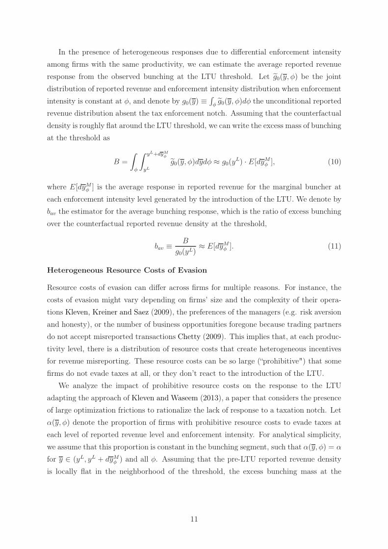
In the presence of heterogeneous responses due to differential enforcement intensity

among firms with the same productivity, we can estimate the average reported revenue

response from the observed bunching at the LTU threshold. Let %g0(y,φ) be the joint

distribution of reported revenue and enforcement intensity distribution when enforcement

intensity is constant at φ, and denote by g0(y) ≡´

φ %g0(y,φ)dφ the unconditional reported

revenue distribution absent the tax enforcement notch. Assuming that the counterfactual

density is roughly flat around the LTU threshold, we can write the excess mass of bunching

at the threshold as

B =

ˆ

φ

ˆ yL+dyMφ

yL%g0(y,φ)dydφ ≈ g0(y

L) · E[dyMφ ], (10)

where E[dyMφ ] is the average response in reported revenue for the marginal buncher at

each enforcement intensity level generated by the introduction of the LTU. We denote by

bav the estimator for the average bunching response, which is the ratio of excess bunching

over the counterfactual reported revenue density at the threshold,

bav ≡B

g0(yL)≈ E[dyMφ ]. (11)

Heterogeneous Resource Costs of Evasion

Resource costs of evasion can differ across firms for multiple reasons. For instance, the

costs of evasion might vary depending on firms’ size and the complexity of their opera-

tions Kleven, Kreiner and Saez (2009), the preferences of the managers (e.g. risk aversion

and honesty), or the number of business opportunities foregone because trading partners

do not accept misreported transactions Chetty (2009). This implies that, at each produc-

tivity level, there is a distribution of resource costs that create heterogeneous incentives

for revenue misreporting. These resource costs can be so large (“prohibitive") that some

firms do not evade taxes at all, or they don’t react to the introduction of the LTU.

We analyze the impact of prohibitive resource costs on the response to the LTU

adapting the approach of Kleven and Waseem (2013), a paper that considers the presence

of large optimization frictions to rationalize the lack of response to a taxation notch. Let

α(y,φ) denote the proportion of firms with prohibitive resource costs to evade taxes at

each level of reported revenue level and enforcement intensity. For analytical simplicity,

we assume that this proportion is constant in the bunching segment, such that α(y,φ) = α

for y ∈ (yL, yL + dyMφ ) and all φ. Assuming that the pre-LTU reported revenue density

is locally flat in the neighborhood of the threshold, the excess bunching mass at the

11

threshold is now given by

Brc =

ˆ

φ

ˆ yL+dyMφ

yL[1− α(y,φ)] · %g0(y,φ)dydφ ≈ g0(y

L) · (1− α) · E[dyMφ ], (12)

where E[dyMφ ] is the average response to the threshold, and (1−α) determines the extent

to which that response is attenuated by resource costs. Considering that any mass in

the bunching segment results from high resource costs, we can estimate the (constant)

proportion of firms with prohibitive costs to react, the “frictioners”, as

α ≡

´ yL+dyMφyL g(y)dy´ yL+dyMφyL g0(y)dy

, (13)

where g(y) is the observed post-LTU reported revenue density and g0(y) is the coun-

terfactual pre-LTU density. We use the approximation in (12) and the estimation of α

to derive a bunching parameter that measures the response to effective tax enforcement

correcting for the attenuation due to resource costs, which we express as

brc ≡B

g0(yL) · (1− α)≈ E[dyMφ ]. (14)

Expression (14) indicates that the larger the number of bunching firms and the smaller the

hole in the bunching range (i.e. higher presence of frictioners) the larger is the response

to effective tax enforcement. This parameter provides a lower bound on the response to

the LTU when the distribution of resource costs is positively related with firm size, and

thus the proportion of frictioners is increasing in the bunching region.15 Instead, when

the LTU creates heterogeneity of enforcement intensity across taxpayers in the bunching

segment, the parameter measures the response by firms most affected by the increase

in monitoring effort. Hence, with an homogeneous distribution of resource costs, the

bunching estimator (14) provides an upper bound on the average response to effective

tax enforcement in the population of firms.

3 Empirical Strategy

This section presents the empirical procedure to estimate the reported revenue response of

firms to a tax enforcement notch [created by the introduction of a LTU]. To quantify this

response, we adapt the techniques from the bunching literature in individual taxation

(Saez, 2010; Chetty et al., 2011; Kleven and Waseem, 2013) to estimate the bunching

15The downward bias is small when firms in the bunching segment have similar/homogenous distribu-tion of resource costs at each productivity level.

12

parameters derived in the previous section. We then introduce an adjustment to quantify

the reaction that would be observed in the absence of high resource costs that constrain

firms’ responses to the notch.

3.1 Standard Bunching Estimator

The basic procedure to estimate the reaction of firms to a LTU relies on constructing

a counterfactual distribution of reported revenue in the absence of a tax enforcement

notch, and comparing it with the observed distribution. To build the counterfactual, we

fit a high-degree polynomial to the observed density, excluding an interval around the

threshold. We discuss below how the excluded interval is determined. Dividing the data

in small bins of width w, we estimate the polynomial regression

Fj =q&

i=0

βi · (yj)i +

yub&

k=ylb

γk · (yj = k) + ηj, (15)

where Fj is the number of firms in bin j, q is the order of the polynomial, yj is the revenue

midpoint of bin j, ylb and yub are the lower and upper bound of the excluded interval

(respectively), and the γk’s are intercept shifters for each of the bins in the excluded

interval. Then, using the estimated coefficients from regression (15), we estimate the

counterfactual distribution of reported revenue, that is,

'Fj =q&

i=0

(βi · (yj)i . (16)

The latter expression excludes the γk shifters to ensure that the counterfactual density

is smooth around the threshold. Comparing this counterfactual density to the observed

distribution we can estimate the excess bunching mass to the left of the threshold (B),

and similarly the missing mass to the right of the threshold (H), given by

(B =yL&

j=ylb

)Fj −'Fj

*≥ 0 and (H =

yub&

j=yL

)'Fj − Fj

*≥ 0. (17)

Determining the lower and upper bounds of the excluded region in a consistent way is

critical for this estimation method to provide credible estimates. We follow the approach

proposed by Kleven and Waseem (2013) to determine these bounds. This procedure

imposes that the areas under both the counterfactual and the observed density have to

be equal, and thus the missing area (H) has to be equal to the excess mass (B). Implicitly,

this is equivalent to assuming that all responses to the tax enforcement notch are on the

intensive margin (i.e., firms don’t go out of business due to the introduction of the LTU,

13

they only adjust their reported revenue). To obtain consistent bunching estimates, we

first fix the lower bound ylb approximately at the point where the shape of the observed

distribution changes due to the bunching response.16 Second, we set the upper bound at

yub ≈ yL and then run regression (15) multiple times, increasing the value of yub by a

small amount after each iteration. When bunching is substantial, the first few iterations

yield large estimates of (B and small estimates of (H . This estimation procedure iterates

until reaching a value of yub such that missing and bunching areas converge, i.e (B = (H .17

Once we have estimates for the number of bunching firms B and the counterfactual

density at the threshold g0(y), we can estimate the bunching parameter b defined in

equation (9). The explicit formula for the estimator is given by

(b =(B+

11+(yL−ylb)/w

,-yL

j=ylb(βi · (yj)i

, (18)

where!1 +

"yL − ylb

#/w

$is the number of excluded bins below the threshold.

Since we apply this estimation to the universe of firms affected by the presence of

the notch, rather than a random sample, there is no sampling error and therefore we

cannot construct the usual confidence intervals. To test whether the point estimates are

statistically significant, we sample the residuals from regression (15) a large number of

times (with replacement) to obtain bootstrapped standard errors.18

3.2 Adjusted Bunching Estimator: Resource Costs

In the theoretical section we derived the parameter brc, which identifies the response to

the LTU that would be observed in the absence of prohibitive resource costs. In order to

estimate this parameter, we need to quantify α, that is, the proportion of firms locating in

the excluded interval"yL, yub

$determined by the (convergence) method compared to the

estimated counterfactual density. We use this measure to reweigh the bunching estimator

in order to obtain the adjusted bunching estimator (brc =!b

1−α . In the presence of a notch,

we can interpret estimates of (brc as an upper bound of the firms’ response to effective

tax enforcement. As before, we calculate standard errors using bootstrapping procedure

described above.19

16Even though there is some discretion in the choice of the lower bound, we show in section 5 that thebunching estimates resulting from a range of values of ylb are fairly stable.

17In the empirical application there is a finite number of bins, so we impose the weaker condition thatthe ratio be “close” to one, i.e. H/B ∈ [0.9, 1.1].

18We thank Michael Best for sharing his Stata code to perform the bootstrapping routine. In all theresults shown below, we perform 200 iterations to obtain the standard errors. Using a larger numberdoes not affect our results.

19Kleven and Waseem (2013) propose a similar method to account for optimization frictions, althoughin their case there is a strictly dominated region in which no taxpayer should locate under any preferences,

14

4 Institutional Context and Data

To test and quantify the predictions of the theoretical framework, we take advantage of

the presence of a tax enforcement notch in Spain. We summarize below the main charac-

teristics of the Spanish Large Taxpayers Unit (LTU), which applies stricter enforcement

intensity on firms above an arbitrary revenue threshold. We also describe two other policy

thresholds relevant for tax administration and the dataset used in our empirical analysis.

4.1 Tax Administration Thresholds: the Spanish LTU

The Spanish tax authority established a LTU (Unidades Regionales de Gestion de Grandes

Empresas) in 1995 to increase its monitoring effort on the largest taxpayers. To define a

“large firm” the tax authority established a threshold at e6 million in annual operating

revenue that has not been modified since then.20 The number of firms in the LTU census

(excluding public companies) increased from 16,713 in 1999 to 34,923 in 2007. Such a

sharp increase was due mainly to strong economic growth and an annual inflation rate

around 3%.21 Despite the fact that the LTU includes only about 2% of all firms that

submit a corporate income tax return, firms in the LTU report about 80% of all taxable

profits and two-thirds of total sales subject to VAT, and they employ around 40% of

private sector wage-earners (AEAT, 1999-2008).

Businesses just above and below the LTU threshold face the same corporate income

tax rates and the same administrative requirements related to invoicing, accounting and

information reporting. Therefore, holding everything else constant, all their transactions

leave the same amount of paper trail. The key difference we exploit in our empirical

strategy is the fact that enforcement intensity is higher for firms above the threshold.

Indeed, the LTU has more human resources to monitor tax returns, allowing it to perform

comprehensive tax audits on approximately 10% of large firms each year, while barely

1% of firms below the threshold are audited (AEAT, 1999-2008). Furthermore, the LTU

makes heavier use of the available technological resources to detect inconsistencies in

firms’ reported transaction by cross-checking tax returns. 22 Overall, the Spanish LTU

because the take-home pay falls as income rises due to the design of the Pakistani income tax. In oursetting, there is no strictly dominated region because there may be heterogeneity in the resource costsof evasion faced by firms.

20The threshold was originally set at 1 billion pesetas, the official currency at the time. The fixedexchange rate is 166.386 pesetas per euro, so the threshold is exactly at e6.010121 million. In 2006, anadditional threshold of e100 million in operating revenue was established to determine eligibility to theCentral Office for Large Firms, a select group of the largest firms within the LTU.

21The overall staff of the tax authority, and the LTU in particular, remained almost constant duringthis period, but the LTU was endowed with better technological resources to monitor the rising numberof taxpayers (AEAT, 1999-2008).

22As an example of its abundance of resources, the LTU has capacity to process electronic VATdeclarations on a monthly basis rather than the quarterly frequency for the rest of firms. This reporting

15

provides quasi-experimental variation in the monitoring effort on large firms with the

same paper trail requirements, allowing us to examine firms’ responses to effective tax

enforcement.

Corporate Income Tax Threshold. The standard rate in the corporate income tax

was 35% of taxable profits in the period 1999-2007. A lower rate of 30% was applied to

firms under a revenue threshold that was modified over time: from e1.5 million in 1999

up to e10 million in 2010 (full details provided in Table A.2). The cutoff for this tax

break overlapped with the LTU threshold in 2004, but was different in the rest of the

years. The lower rate was applied only to the first e90,121 of taxable profits (e120,202

since 2005) creating a notch for eligible firms with low taxable profits, and a kink for

those with high profits.

External Audit and Abbreviated Returns Threshold. Firms are required by law

to have their annual accounts audited by an external private firm if they fulfill two of

the following criteria for two consecutive years: (i) annual revenue above e4.75 million;

(ii) total assets above e2.4 million;23 and (iii) more than 50 employees on average during

the year. These criteria also determine whether a firm can use the abbreviated form of

the corporate income tax return, rather than the standard (long) version. These require-

ments create compliance costs,24 and the private audit information could complement tax

enforcement because auditors face legal responsibility if any misreporting is found.

4.2 Data

In the empirical analysis we use data from financial statements that, according to the

law, all Spanish firms must submit to the Commercial Registry (Registro Mercantil Cen-

tral). The micro-data compiled and digitalized by Amadeus, a European-level data set

published by Bureau van Dijk, provides information for each firm such as business name,

location (5-digit post code), sector of activity (4-digit NAICS25 code), 26 balance sheet

items, 26 profit and loss account items, and 32 standard financial ratios.26 Table A.4 in

requirement might impose a minor compliance cost to LTU-eligible firms compared to ineligible ones.23The revenue limit was originally 790 million pesetas (e4.748 million), and the assets limit was 395

million pesetas (e2.374 million).24The yearly fee charged by private audit firms is in the range e10,000 - e30,000 for firms with revenue

close to e4.75 million, a small but non-negligible expenditure (0.2 to 0.6% of total revenue, but 4 to 12%of reported profits on average).

25NAICS stands for North-American Industry Classification System.26For the purposes of this paper, we accessed the online version of Amadeus in November 2011. Since

the dataset is continuously updated, the information currently available in the online version may havesuffered some changes, e.g., businesses that are inactive for four consecutive years are dropped from thedataset.

16

the online appendix compares the number of firms in the Amadeus data to the number of

corporate tax returns reflected in official statistics, by levels of operating revenue. Very

small firms are underrepresented in the data because they tend to submit their financial

statements on paper rather than electronically, in which case Amadeus is less likely to

include them. However, there is complete data for more than 80% of firms with reported

revenue between e3 and e9 million, the range that is most interesting for our empirical

analysis. Given that there is information on almost the universe of firms in the relevant

size range, this dataset is well suited to examine firms’ responses to the Spanish LTU.

The dataset contains information on the annual net revenue from sales, the key vari-

able used to determine whether firms are eligible to the LTU and also the other policy

thresholds discussed above. Firms have no incentive to report different amounts in their

tax returns, because it would be extremely easy for the tax authority to cross-check the

information. Hence, the annual revenue figure in the financial statements must match

exactly with tax returns. The dataset also includes data on the two largest categories

of firms expenditures: materials, which accounts for the cost of all raw materials and

services purchased by the firm in the production process; and labor, which accounts for

the total wage bill of a firm, including social security contributions charged on employees.

The average number of employees reported during the fiscal year (same as the calendar

year) is also available for the vast majority of firms.27

One important advantage of this dataset is its longitudinal structure, which allows us

to study the dynamic behavior of firms around the threshold over time. One potential

advantage of using financial statements instead of tax returns is the possibility of observ-

ing multiple margins of response in a single dataset.28 We explore dynamic behavior in

subsection 5.3 and the anatomy of the response to the LTU threshold in subsection 5.4.

5 Results

We first document and quantify the reaction of Spanish firms to the notch in effective tax

enforcement created by the introduction of a LTU. Second, we examine the heterogeneity

of this response across sectors of activity and other dimensions of firm size such as the

number of employees. The analysis provides insights on the effectiveness of monitoring

effort depending on firm characteristics, and how resource costs of evasion attenuate the

observed response. Third, we study the dynamic behavior of firms near the threshold

to assess the degree of persistence in bunching behavior. Finally, we consider changes in

27This variable is missing for about 20% of the firms that report their total sales and material inputs.However, we do not detect a different proportion of missing values around the thresholds of interest.

28This is often not possible with administrative tax returns, because confidentiality rules preventresearchers from linking firms across different data sources.

17

reported input expenditures as an alternative margin of response for firms.

5.1 Static Bunching Estimation

Figure 2 shows the empirical distribution of reported revenue for Spanish firms in the

period 1999-2007, using micro-data from Amadeus. We focus on firms in the range

between e3 and e9 million, centering the graph around the LTU threshold. There is

substantial bunching of firms just below the LTU threshold, indicating that a significant

number of firms attempt to avoid stricter tax enforcement.29 Figure 3 shows the coun-

terfactual and empirical distributions of revenue, overlaid. Implementing the bunching

estimation procedure derived in section 3, we obtain a point estimate (bav = 0.101, which

is statistically different from zero at the 1% level (the bootstrapped standard error is

0.007). This point estimate implies that firms reduce their reported revenue by about

e101,000 (approximately 1.7% of total reported revenue) on average in response to the

tax enforcement notch. As predicted by our theoretical framework, there is no “hole”

in the distribution to the right of the LTU threshold, just a small dip. We hypothesize

that firms face heterogeneous resource costs of evasion, which attenuates the bunching

response by preventing some firms from responding. Using the adjusted bunching esti-

mator, we obtain (brc = 0.593 (s.e. 0.122), implying that the marginal bunching firm with

low adjustment costs reduces its reported revenue by about e593,000 (almost 10% of

total reported revenue).

Robustness checks. We address several potential issues that may be raised about

the robustness of the static bunching estimates. First, pooling several annual cross-

sections together increases the effective sample size allowing us to obtain more precise

estimates, but it could mask differences in the response across years. Table 1 shows

that bunching estimates are all significant and of similar magnitude in every year.30

We analyze the dynamic patterns of firm behavior in subsection 5.3 below. Second,

the observed response could be affected by other size-dependent policies, such as the

corporate income tax benefit for small firms discussed in the previous section. We do

not find any evidence of bunching in response to this tax break over time.31 The lack of

reaction to a five-percentage-point reduction in the corporate income tax rate (besides

additional tax credits and fiscal advantages), is remarkable in a context where firms

29There is another spike in the distribution just below the External Audit threshold. This spike issmaller in magnitude and more difficult to interpret because the criteria to determine eligibility involvetwo other variables apart from reported revenue (employees and assets), as discussed in section 4. Forthese reasons, in the remainder of the paper we focus on the response to the LTU threshold.

30The annual histograms are shown in Figure A.2 in the online appendix.31As explained in section 4, this threshold changes over time. The distribution of reported revenue

under each of the thresholds is shown in Figure A.1 in the online appendix.

18

respond strongly to a discontinuity in tax enforcement intensity. This evidence indicates

that the perceived impact of strict tax enforcement is large for a significant proportion of

Spanish firms. Third, the arbitrary selection of the lower bound of the excluded interval

ylb could bias the estimation. We perform a sensitivity analysis of our main estimates

selecting different values for the lower bound of the excluded region around our preferred

value of e5.4 million, such that ylb = {5.2, ..., 5.6}. Table 2 reports the results for the

pooled 1999-2007 data. The resulting upper bound yub is quite stable between e6.62

and e6.78 million. Similarly, point estimates for (bav are all in the interval (0.097, 0.102)

and those of (brc are in the interval (0.537, 0.621). Overall, we conclude that any sensible

choice of the lower bound ylb yields similar estimates of the bunching response.

5.2 Heterogeneous Responses: Deterrence and Resource Costs

According to the theoretical framework, firms face different incentives to misreport their

revenue depending on (i) the deterrence effect of tax enforcement, which is determined

by the tax authority’s ability to detect tax evasion (i.e. the traceability of the paper

trail); and (ii) the costs of such evasion, both direct and indirect, incurred by firms. To

provide insights on the impact of these factors on tax compliance, we analyze evidence

on cross-sectional differences in the behavioral response of firms to the tax enforcement

notch created by the LTU.

Deterrence Effect across Sectors of Activity. On the deterrence component, we

expect a larger response to the LTU for firms in the middle of the value chain, which

sell mostly to other firms, than those at the last stage of the chain, which sell mostly to

final consumers. Intuitively, it is much easier to detect misreported intermediate input

sales than it is to detect unreported sales to final consumers, because the latter have

no incentive to keep a receipt. Since we lack transaction-level data for each firm, we

define 10 sectors of activity as an indicator of firms’ position in the value chain.32 We

obtain the percentage of sales made to final consumers in each sector from the input-

output tables of the Spanish economy in the year 2000, published by the Institute of

National Statistics (INE). Figure 4 plots this percentage (in the horizontal axis) against

the bunching estimates by sector (measured by (bav, vertical axis). The relationship is

downward-sloping, suggesting that the incentive to remain under the LTU threshold is

stronger in sectors where a low percentage of sales is made to final consumers. On the

top-left corner, heavy manufacturing, construction and building contractors, all of them

with less than 10% of sales going to final consumers, present high bunching estimates

(between 0.09 and 0.15). On the bottom-right corner, retailers, restaurants and hotels,

32Details about how we define each of the sectors can be found in the online appendix.

19

which obtain more than 80% of their revenue from sales to final consumers, have much

lower bunching response (between 0.04 and 0.07) to the same nominal revenue threshold.

All the bunching estimates are significantly different from zero except for restaurants and

hotels. The counterfactual and empirical distributions of revenue in the relevant sectors

are shown in Figure 5, and all the point estimates are reported in Table 3.

The negative correlation between a high share of hard-to-trace transactions and the

size of the bunching response at the enforcement notch is consistent with the predictions

of our model. Holding the information requirements constant, the same increase in mon-

itoring resources yields different effective enforcement intensities across firms depending

on the traceability of their paper trail. The empirical results imply that the deterrence

effect associated to higher monitoring resources is most effective for firms whose misre-

ported transactions are easier to detect. In contrast, the increase in monitoring resources

is less binding for firms that sell mostly to final consumers. Overall, the evidence indi-

cates that paper trail requirements and monitoring effort are complements, and thus it

is the interaction between these two elements that yields higher tax compliance.

Resource Costs and Firm Size. As shown above, a significant subset of firms report

revenue just above the LTU threshold. We associate this lack of response to the presence

of prohibitive costs that prevent firms from misreporting their revenue. Measuring re-

source costs of evasion is extremely difficult, because some of these costs are indirect (e.g.,

foregoing business opportunities) and others are hard to separate from regular expenses

(e.g., hiring tax advisers). Instead of quantifying these costs, we take advantage of our

empirical application to test whether they are related with the size and complexity of

firms’ operations Kleven, Kreiner and Saez (2009).

Our empirical setting provides variation in tax enforcement intensity for firms with

similar size in terms of reported revenue. As discussed above, the change in tax en-

forcement intensity is related with the position of firms in the value chain, creating high

incentives to bunch for firms with easily traceable transactions. Bunching estimates by

sector of activity, which control for differences in tax enforcement effectiveness, also show

that the lack of response due to resource costs, α, is significant for sectors with large re-

sponses to the LTU. These results indicate that firm size, measured by reported revenue,

is related with the magnitude of resource costs preventing firms to evade even when the

tax authority undertakes a low effort to monitor their tax returns.

As a complementary analysis, we proxy firms’ complexity using other dimensions of

firms size, such as the number of employees and the stock of fixed assets. For a given

level of reported revenue, we expect firms with more employees and/or fixed assets to

exhibit lower bunching at the LTU threshold because they face higher resource costs of

20

evasion. The results in the bottom panel of Table 3 show that bunching is stronger for

firms with fewer than 50 employees, and for firms with less than e2,4 million in assets.33

These results indicate that additional firm’s complexity contributes to increase its resource

costs preventing them to react to the LTU. We conclude that, as predicted by Kleven,

Kreiner and Saez (2009), large and more complex firms bear considerable resource costs

that result in high tax compliance with low monitoring effort for a significant proportion

of firms.

5.3 Dynamic Firm Behavior

The bunching analysis imposes a static perspective by pooling observations from different

years. This means that many firms appear in the data in multiple years, but the graph-

ical analysis does not control for potential autocorrelation. A potential issue with this

estimation strategy is that persistent bunching behavior by a small group of firms could

bias our cross-sectional estimates upward.34 We present below some descriptive evidence

of firms’ growth patterns and analyze the extent of bunching persistence to address this

concern.

First, we compare the behavior of growing firms, defined as those reporting higher

revenue in the current year than the previous year, and shrinking firms. Figure 6 shows

that growing firms bunch very significantly at the threshold, whereas shrinking firms

barely respond. This seems to indicate that firms perceive crossing the LTU threshold

as a fixed cost, for example because they need to change the way they operate under

stricter tax monitoring. The strong reaction of growing firms is further documented in

Figure 7, which shows median revenue growth compared to current revenue.35 Median

growth rates are close to 5% for most firms in the e3-e9 range, except for a sharp decline

for firms approaching the threshold from below (i.e., those with revenue between e5-e6

million). Overall, these patterns suggest that as small firms approach the threshold from

below, a subset of them slows down their growth to avoid crossing it.

In order to assess more directly the hypothesis that there is a small number of per-

sistent bunchers, we perform an additional test suggested by Marx (2012). The idea is

to estimate whether firms are more likely to stay in the bunching region than in any

other part of the revenue distribution. In order to precisely define the bunching region,

we divide reported revenues in equally-sized bins of e601,012 (ten times wider than the

33We choose these reference thresholds because they are two of the eligibility criteria in the ExternalAudit threshold.

34It is important to keep in mind that the LTU notch was fixed in nominal terms throughout theperiod under study, while inflation averaged 3% per year and real annual growth was close to 4%. Thus,the notch moved down about 27% in real terms between 1999 and 2007.

35We define median growth rate in each revenue bin as Σimedian (ln (yi,t+1)− ln (yi,t)). We usemedian instead of average growth rates because the latter take many extreme values.

21

bins in the histogram of reported revenue). We define the “bunching bin” as the range of

reported revenue between e5.41-e6.01 million.36 We then compare the fraction of firms

that remain in the bunching bin after h years to the fraction that remain in other revenue

bins, where h = {1, 2, ..., 6}. Formally, we estimate the equation

Prob!bin (yit) = bin

"yi,t+h

#$= α+ βBunchBinit + yit + y2it + εit, (19)

where the dependent variable is the fraction of firms that report revenue (yit) in the

same bin in years t and t + h, and the dummy variable BunchBinit takes value one if

yit ∈ (5.4, 6.0]. We add a quadratic polynomial in current reported revenue as a way to

control for the counterfactual probability that firms remain in a given revenue bin.37 In

the actual regression, we use the distance to the threshold instead of the actual level of

reported revenue. This allows us to interpret the constant term α as the fraction of firms

near the notch expected to remain at their current revenue level h years from now.

Figure 8 presents the results graphically. The top-left graph shows the probability that

firms remain in the same revenue bin after one year. This probability decreases smoothly

from about 30% in the range yit ∈ (3.0, 3.6) to 12% in the range yit ∈ (9.4, 10.0). However,

there is a clear deviation from the trend at the bunching bin, where the proportion of

firms that stay is 26.5%, compared to the 20.7% predicted by the counterfactual. This

means that a firm in the bunching bin is 28 percent (5.8 percentage points) more likely

to remain in the same revenue bin one year later. The regression results for all values

of h are summarized in Table 4. The coefficient on the BunchBin dummy is significant

at the 5% level for all lags up to six years, but it is only economically significant for the

short lags (up to two or three years). This short-term persistence suggests that bunching

is generated by a group of growing of firms that changes over time. We conclude that

the static bunching estimates are unlikely to be biased due to this short-term bunching

persistence.

5.4 Anatomy of the Response: Input Misreporting below the

LTU Threshold

We analyze the relative use of inputs reported by firms to learn about the mechanism

behind firms’ responses to stricter tax enforcement. To obtain testable hypothesis, we

derive theoretical predictions on the average reported ratios of tax-deductible input ex-

penditures over revenue around the LTU threshold (see section B in the online appendix

36The results are qualitatively similar for smaller bin widths, such as e180,000 or e60,101. Resultsavailable upon request.

37In the data, the probability of staying in a given revenue bin decreases with revenue for all values ofh, because the equal-sized bins are proportionally smaller as we move to higher revenue levels.

22

for a full derivation of the model). We obtain different predictions depending on whether

firms’ reaction is due to real (i.e. lower output) or evasion (increase of concealed revenue)

adjustments. We enrich the range of predictions with the insights from an extended

model that considers the possibility that firms have also incentives to misreport their

inputs expenditures to evade their tax liabilities in the presence of multiple taxes (i.e.

value-added tax, payroll taxes and corporate income tax). The set of predictions can

be tested with simple graphical evidence from our dataset showing the average reported

ratios of labor and material expenditures over revenue around the LTU threshold. We

use these tests to rule out mechanisms of the reaction consistent with the theory, rather

to identify causal effects of tax enforcement on firms’ expenditures reporting.

Empirical Evidence and Theoretical Predictions. The top-left panel of Figure

9 plots the average reported ratio of material input expenditures over revenue on the

vertical axis and reported revenue in the horizontal axis, both measured in year t, for

the period 1999-2007. Each bin is e120,202 wide, which is twice as wide as the bins in

the reported revenue histograms described above.38 The ratio slopes up in the reported

revenue range between e3 and e9 millions with a concave shape, indicating that firms

with larger revenue use an increasingly higher proportion of material inputs. The relative

use of material inputs increases smoothly in reported revenue until reaching the LTU

threshold where jumps sharply downwards by about two percentage points (from 66%

to 64%). The top-right panel of Figure 9 shows the same evidence for the reported

ratio of labor expenditures over revenue. The pattern in this case is approximately the

reverse: the ratio slopes down smoothly in reported revenue with an upward jump of one

percentage point (from 15% to 16%) at the LTU threshold.

According to our theoretical predictions (see section B in the online appendix), these

patterns are not compatible with a real response to the LTU threshold. In that case, the

reduction of production by the bunchers should have implied lower use of both inputs,

resulting in a upward jump of both expenditure ratios at the threshold. The empirical

patterns instead can be rationalized with an evasion response by buncher firms which

also misreport their expenditures. As we show in section B in the online appendix,

both CIT and VAT create incentives for evader firms to inflate material expenditures in

order to claim larger tax credits. Moreover, those firms have incentives to hide labor

expenditures to reduce their payroll tax liability and avoid the regulatory costs of hiring

workers. Hence, when firms that misreport expenditures conceal revenue to bunch below

the threshold, the model predicts a downward (upward) jump in the ratio of materials

38Wider bins reduce the amount of noise in the figures presented below. We do not adjust for inflationbecause the outcome variable is a ratio of two nominal amounts. We implicitly assume that the inflationon the output good is the same as for inputs.

23

(labor) expenditures over revenue just at the LTU threshold.

A potential issue that may be raised is that labor-intensive firms could be less likely

to bunch because prohibitive resource costs are strongly related with the number of em-

ployees. This would mechanically yield lower average labor expenditures in the interval

just below the threshold creating discontinuities in the expenditures ratio due to a com-

position effect in the data. The bottom panels of Figure 9 provide a more disaggregated

picture of labor expenditures that rejects this hypothesis. On the left, we do not observe

a discontinuity of the average number of employees at the threshold. Instead, the right

panel plots average gross wages (total wage bill divided by the number of employees),

which features an upward jump at the threshold. This means that most of the shift in

labor expenditures at the enforcement threshold is due to different reported wages and

not a different number of employees. This evidence seems more consistent with the in-

puts evasion channel than with the composition-effect hypothesis. Even though this is

not a definitive test, we take it as suggestive evidence that firms that manipulate their

reported revenue to avoid the stricter tax enforcement by the LTU also misreport their

input expenditures in order to evade multiple taxes.

6 Concluding Remarks

In this paper, we have investigated the effectiveness of exploiting information trails gen-

erated by business activities to enforce taxes. We first derive theoretical predictions on

firms’ responses to increases in the tax authority resources to verify the transactions

reported by firms. We then test the predictions on firms’ tax compliance using quasi-

experimental variation in monitoring effort provided by the Large Taxpayers Unit (LTU)

in Spain.

The empirical results show that firms react to avoid being under more effective tax

enforcement reducing their reported revenue. This reaction is heterogeneous among firms

depending on the traceability of their transactions, indicating the complementarity be-

tween monitoring effort and information requirements to reach tax compliance. In partic-

ular, we find larger reaction in sectors that sell intermediate goods where the information

trail is easier to verify with more monitoring resources. Finally, we document that firms

are able to misreport both labor expenditures and material acquisitions to evade taxes

when the capacity to verify those transactions is low.

The results of the paper highlight the relevance of monitoring the information trail

created by firms to ensure tax compliance. Firms are not only the third-party agent that

helps to prevent individuals’ tax evasion, but tax authorities must devote resources to

verify their activities to reach effective tax enforcement.

24

References

AEAT. 1999-2008. “Memoria de Administración Tributaria.” Spanish Tax Authority

(Agencia Estatal de Administración Tributaria).

Allingham, Michael, and Agnar Sandmo. 1972. “Income tax evasion: A theoretical

analysis.” Journal of Public Economics, 1: 323–338.

Amadeus. 1999-2007. “Database of comparable financial information for European com-

panies, published by Bureau van Dijk.”

Bastani, Spencer, and Hakan Selin. 2014. “Bunching and Non-Bunching at Kink

Points of the Swedish Tax Schedule.” Journal of Public Economics, 109: 36–49.

Best, Michael C. 2013. “Salary Misreporting and the Role of Firms in Workers’ Re-

sponse to Taxes: Evidence from Pakistan.” London School of Economics.

Best, Michael C., and Henrik J. Kleven. 2013. “Housing Market Responses to

Transaction Taxes: Evidence from Notches and Stimulus in the UK.” London School

of Economics.

Carrillo, Paul, Monica Singhal, and Dina Pomeranz. 2014. “Tax Me if You Can:

Evidence on Firm Misreporting and Evasion Substitution.” Harvard Kennedy School.

Chetty, Raj. 2009. “Sufficient Statistics for Welfare Analysis: A Bridge Between Struc-

tural and Reduced-Form Analysis.” Annual Review of Economics, 1: 451–488.

Chetty, Raj, John Friedman, and Emmanuel Saez. 2013. “Using Differences in

Knowledge Across Neighborhoods to Uncover the Impacts of the EITC on Earnings.”

American Economic Review, 103(7): 2683–2721.

Chetty, Raj, John Friedman, Tore Olsen, and Luigi Pistaferri. 2011. “Adjustment

Costs, Firm Responses, and Micro vs. Macro Labor Supply Elasticities: Evidence from

Danish Tax Records.” Quarterly Journal of Economics, 126: 749–804.

Christensen, Kevin, Robert Cline, and Tom Neubig. 2001. “Total Corporate

Taxation: "Hidden", Above-the-Line, Non-Income Taxes.” National Tax Journal,

LIV(3): 495–506.

Devereux, Michael, Li Liu, and Simon Loretz. 2014. “The Elasticity of Corporate

Taxable Income: New Evidence from UK Tax Records.” American Economic Journal:

Economic Policy, 6(2): forthcoming.

25

Garicano, Luis, Claire LeLarge, and John van Reenen. 2013. “Firm Size Dis-

trotions and the Productivity Distribution: Evidence from France.” NBER Working

Paper 18841.

Gordon, Roger, and Wei Li. 2009. “Tax Structures in Developing Countries, Many

Puzzles and a Possible Explanation.” Journal of Public Economics, 93: 855–866.

Guner, Nezih, Gustavo Ventura, and Yi Xu. 2008. “Macroeconomic Implications

of Size-Dependent Policies.” Review of Economic Dynamics, 11: 721–744.

IEF. 2011. “Evolución del Sistema Fiscal Español: 1978-2010.” Instituto de Estudios

Fiscales.

IMF. 2002. “Improving Large Taxpayers’ Compliance: A Review of Country Experience.”

International Monetary Fund, Washington DC. Team led by Katherine Baer.

Kleven, Henrik, and Mazhar Waseem. 2013. “Using Notches to Uncover Optimiza-

tion Frictions and Structural Elasticities: Theory and Evidence from Pakistan.” forth-

coming at the Quarterly Journal of Economics.

Kleven, Henrik, Klaus Kreiner, and Emmanuel Saez. 2009. “Why Can Modern

Governments Tax So Much? An Agency Model of Firms as Fiscal Intermediaries.”

NBER Working Paper 15218.

Kleven, Henrik, Martin Knudsen, Claus Kreiner, Soren Pedersen, and Em-

manuel Saez. 2011. “Unable of Unwilling to Cheat? Evidence from a Tax Audit

Experiment in Denmark.” Econometrica, 79(3): 651–692.

Kopczuk, Wojciech, and David J. Munroe. forthcoming. “Mansion Tax: The Effect

of Transfer Taxes on the Residential Real Estate Market.” American Economic Journal:

Economic Policy.

Kopczuk, Wojciech, and Joel Slemrod. 2006. “Putting Firms into Optimal Tax

Theory.” American Economic Review, Papers and Proceedings, 96(2): 130–134.

Kumler, Todd, Eric Verhoogen, and Judith Frias. 2012. “Enlisting Workers in

Monitoring Firms: Payroll Tax Compliance in Mexico.”

Marx, Benjamin. 2012. “Regulatory Hurdles and Growth of Charitable Contributions:

Evidence from a Dynamic Bunching Design.” Columbia University.

OECD. 2011. “Tax Administration in OECD and Selected non-OECD Countries: Com-

parative Information Series (2010).” Organisation for Economic Co-operation and De-

velopment.

26

Onji, Kazuki. 2009. “The response of firms to eligibility thresholds: Evidence from the

Japanese value-added tax.” Journal of Public Economics, 93: 766–775.

Paula, Áureo De, and José Scheinkman. 2010. “Value-Added Taxes, Chain Effects,

and Informality.” American Economic Journal: Macroeconomics, 2: 195–221.

Pomeranz, Dina. 2013. “No Taxation Without Information: Deterrence and Self-

Enforcement in the Value-Added Tax.” Harvard Business School Working Paper 13-057.

Restuccia, Diego, and Richard Rogerson. 2008. “Policy Distortions and Aggre-

gate Productivity with Heterogeneous Establishments.” Review of Economic Dynamics,

11: 707–720.

Saez, Emmanuel. 2010. “Do Taxpayers Bunch at Kink Points?” American Economic

Journal: Economic Policy, 2(3): 180–212.

Slemrod, Joel. 2010. “Buenas Notches: Lines and Notches in Tax System Design.”

University of Michigan.

Slemrod, Joel, and Christian Gillitzer. 2014. Tax Systems. Cambridge, MA:MIT

Press.

Slemrod, Joel, Marsha Blumenthal, and Charles Christian. 2001. “Taxpayer

Response to an Increased Probability of Audit: Evidence from a Controlled Experiment

in Minnesota.” Journal of Public Economics, 79: 455–483.

Yaniv, Gideon. 1988. “Withholding and Non-Withheld Tax Evasion.” Journal of Public

Economics, 35: 183–204.

Yitzhaki, Shlomo. 1974. “A Note on "Income Tax Evasion: A Theoretical Analysis".”

Journal of Public Economics, 3(2): 201–202.

27

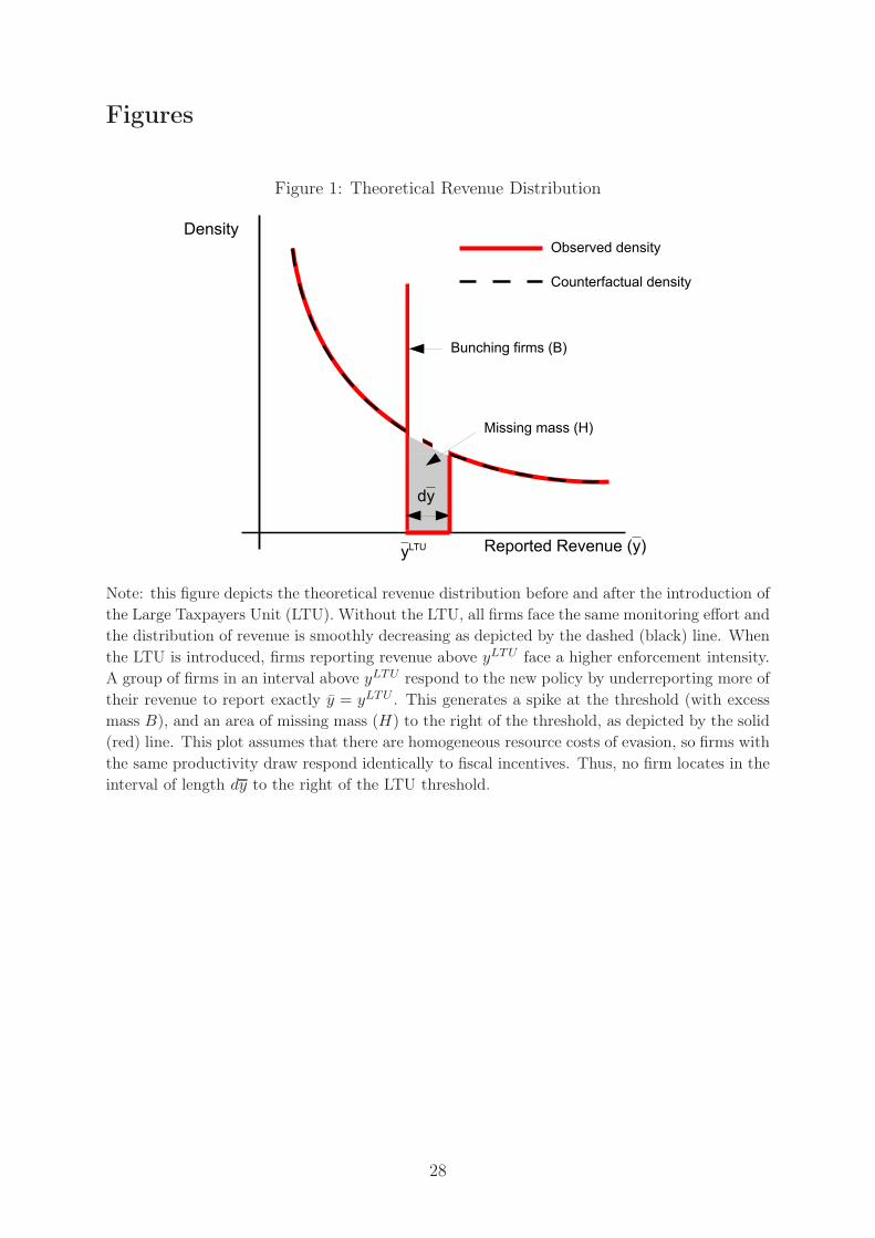
Figures

Figure 1: Theoretical Revenue Distribution

!"#$%&#'()&*+,(-!.

/&,,&#'(+0,,(-1.

23,4*546(64#,&78

9:"#74*)0$7"0;(64#,&78

<4#,&78

=4>:*746(=454#"4(-8.

68

8?@A

Note: this figure depicts the theoretical revenue distribution before and after the introduction ofthe Large Taxpayers Unit (LTU). Without the LTU, all firms face the same monitoring effort andthe distribution of revenue is smoothly decreasing as depicted by the dashed (black) line. When

the LTU is introduced, firms reporting revenue above yLTU face a higher enforcement intensity.A group of firms in an interval above yLTU respond to the new policy by underreporting more of

their revenue to report exactly y = yLTU . This generates a spike at the threshold (with excessmass B), and an area of missing mass (H) to the right of the threshold, as depicted by the solid(red) line. This plot assumes that there are homogeneous resource costs of evasion, so firms with

the same productivity draw respond identically to fiscal incentives. Thus, no firm locates in theinterval of length dy to the right of the LTU threshold.

28

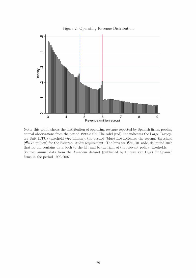
Figure 2: Operating Revenue Distribution

0.1

.2.3

.4.5

Den

sity

3 4 5 6 7 8 9Revenue (million euros)

Note: this graph shows the distribution of operating revenue reported by Spanish firms, poolingannual observations from the period 1999-2007. The solid (red) line indicates the Large Taxpay-ers Unit (LTU) threshold (e6 million); the dashed (blue) line indicates the revenue threshold(e4.75 million) for the External Audit requirement. The bins are e60,101 wide, delimited suchthat no bin contains data both to the left and to the right of the relevant policy thresholds.

Source: annual data from the Amadeus dataset (published by Bureau van Dijk) for Spanishfirms in the period 1999-2007.

29

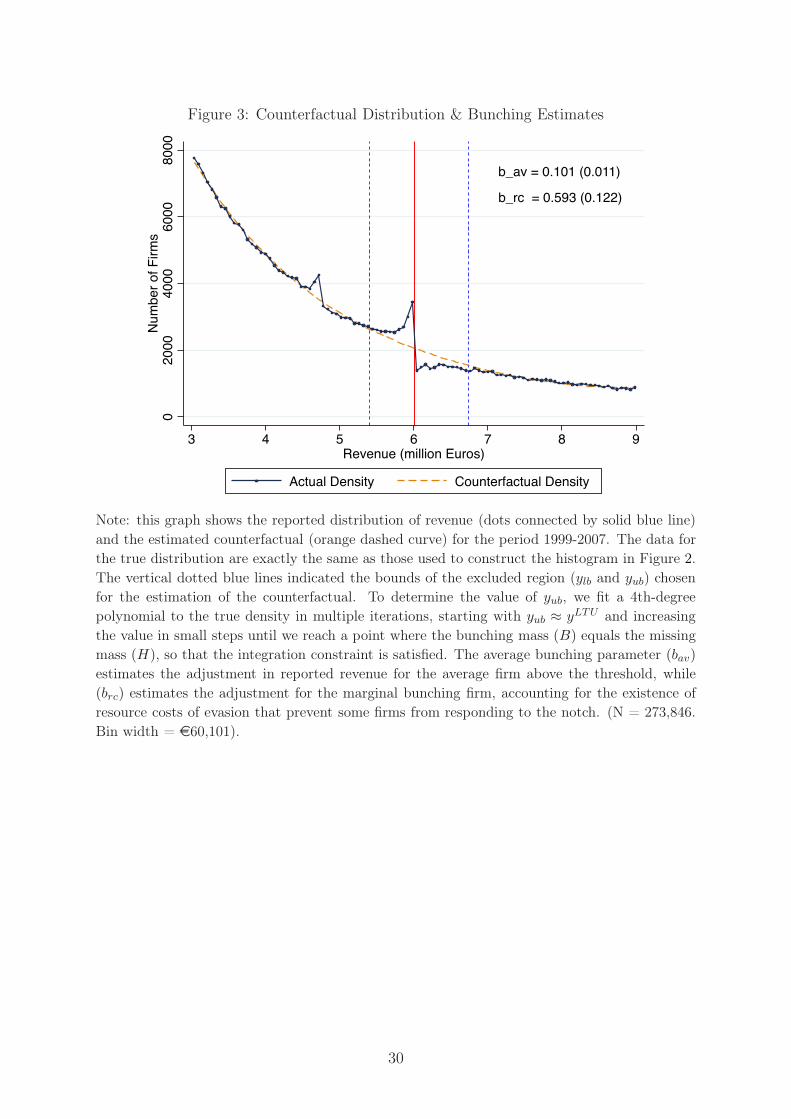
Figure 3: Counterfactual Distribution & Bunching Estimates

b_av = 0.101 (0.011)

b_rc = 0.593 (0.122)

020

0040

0060

0080

00N

umbe

r of F

irms

3 4 5 6 7 8 9Revenue (million Euros)

Actual Density Counterfactual Density

Note: this graph shows the reported distribution of revenue (dots connected by solid blue line)

and the estimated counterfactual (orange dashed curve) for the period 1999-2007. The data forthe true distribution are exactly the same as those used to construct the histogram in Figure 2.

The vertical dotted blue lines indicated the bounds of the excluded region (ylb and yub) chosenfor the estimation of the counterfactual. To determine the value of yub, we fit a 4th-degreepolynomial to the true density in multiple iterations, starting with yub ≈ yLTU and increasing

the value in small steps until we reach a point where the bunching mass (B) equals the missingmass (H), so that the integration constraint is satisfied. The average bunching parameter (bav)estimates the adjustment in reported revenue for the average firm above the threshold, while

(brc) estimates the adjustment for the marginal bunching firm, accounting for the existence ofresource costs of evasion that prevent some firms from responding to the notch. (N = 273,846.

Bin width = e60,101).

30

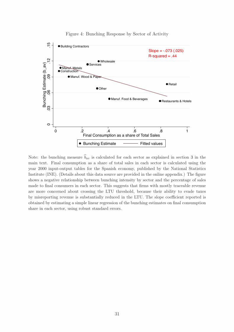
Figure 4: Bunching Response by Sector of Activity

Construction

Building Contractors

Manuf. Food & Beverages

Manuf. Wood & Paper

Manuf. Metals

Wholesale

Retail

Restaurants & Hotels

Services

Other

Slope = -.073 (.025)R-squared = .44

0.0

3.0

6.0

9.1

2.1

5Bu

nchi

ng E

stim

ate

(b_a

v)

0 .2 .4 .6 .8 1Final Consumption as a share of Total Sales

Bunching Estimate Fitted values

Note: the bunching measure (bav is calculated for each sector as explained in section 3 in themain text. Final consumption as a share of total sales in each sector is calculated using theyear 2000 input-output tables for the Spanish economy, published by the National Statistics

Institute (INE). (Details about this data source are provided in the online appendix.) The figureshows a negative relationship between bunching intensity by sector and the percentage of salesmade to final consumers in each sector. This suggests that firms with mostly traceable revenue

are more concerned about crossing the LTU threshold, because their ability to evade taxesby misreporting revenue is substantially reduced in the LTU. The slope coefficient reported is

obtained by estimating a simple linear regression of the bunching estimates on final consumptionshare in each sector, using robust standard errors.

31

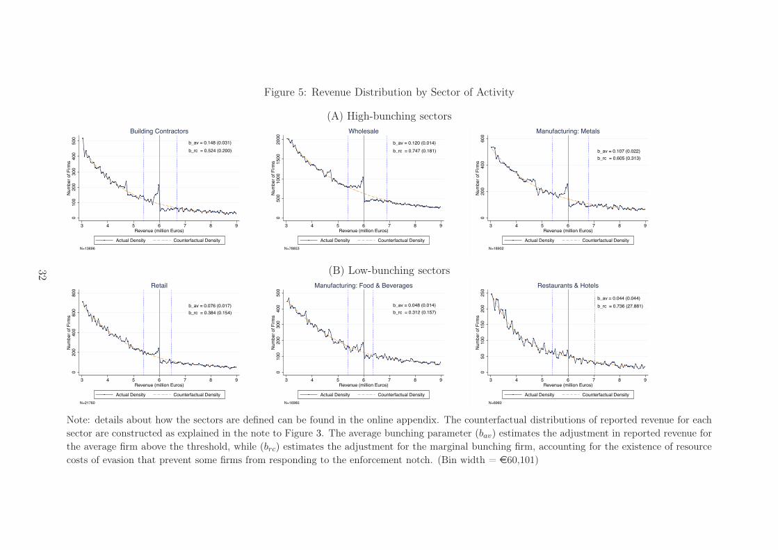
Figure 5: Revenue Distribution by Sector of Activity

(A) High-bunching sectors

b_av = 0.148 (0.031)b_rc = 0.524 (0.200)

010

020

030

040

050

0N

umbe

r of F

irms

3 4 5 6 7 8 9Revenue (million Euros)

Actual Density Counterfactual DensityN=13696

Building Contractorsb_av = 0.120 (0.014)b_rc = 0.747 (0.181)

050

010

0015

0020

00N

umbe

r of F

irms

3 4 5 6 7 8 9Revenue (million Euros)

Actual Density Counterfactual DensityN=78853

Wholesale

b_av = 0.107 (0.022)b_rc = 0.605 (0.313)

020

040

060

0N

umbe

r of F

irms

3 4 5 6 7 8 9Revenue (million Euros)

Actual Density Counterfactual DensityN=18902

Manufacturing: Metals

(B) Low-bunching sectors

b_av = 0.076 (0.017)b_rc = 0.384 (0.154)

020

040

060

080

0N

umbe

r of F

irms

3 4 5 6 7 8 9Revenue (million Euros)

Actual Density Counterfactual DensityN=21760

Retail

b_av = 0.048 (0.014)b_rc = 0.312 (0.157)

010

020

030

040

050

0N

umbe

r of F

irms

3 4 5 6 7 8 9Revenue (million Euros)

Actual Density Counterfactual DensityN=16985

Manufacturing: Food & Beverages

b_av = 0.044 (0.044)b_rc = 0.736 (27.881)

050

100

150

200

250

Num

ber o

f Firm

s

3 4 5 6 7 8 9Revenue (million Euros)

Actual Density Counterfactual DensityN=6960

Restaurants & Hotels

Note: details about how the sectors are defined can be found in the online appendix. The counterfactual distributions of reported revenue for eachsector are constructed as explained in the note to Figure 3. The average bunching parameter (bav) estimates the adjustment in reported revenue forthe average firm above the threshold, while (brc) estimates the adjustment for the marginal bunching firm, accounting for the existence of resource

costs of evasion that prevent some firms from responding to the enforcement notch. (Bin width = e60,101)

32

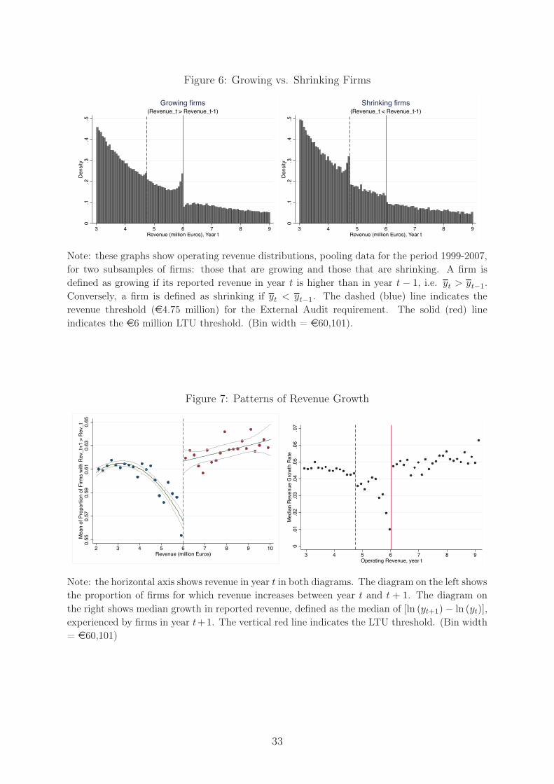
Figure 6: Growing vs. Shrinking Firms0

.1.2

.3.4

.5D

ensi

ty

3 4 5 6 7 8 9Revenue (million Euros), Year t

(Revenue_t > Revenue_t-1)Growing firms

0.1

.2.3

.4.5

Den

sity

3 4 5 6 7 8 9Revenue (million Euros), Year t

(Revenue_t < Revenue_t-1)Shrinking firms

Note: these graphs show operating revenue distributions, pooling data for the period 1999-2007,for two subsamples of firms: those that are growing and those that are shrinking. A firm isdefined as growing if its reported revenue in year t is higher than in year t − 1, i.e. yt > yt−1.

Conversely, a firm is defined as shrinking if yt < yt−1. The dashed (blue) line indicates therevenue threshold (e4.75 million) for the External Audit requirement. The solid (red) line

indicates the e6 million LTU threshold. (Bin width = e60,101).

Figure 7: Patterns of Revenue Growth

0.55

0.57

0.59

0.61

0.63

0.65

Mea

n of

Pro

porti

on o

f Firm

s w

ith R

ev_t

+1 >

Rev

_t

2 3 4 5 6 7 8 9 10Revenue (million Euros)

0.0

1.0

2.0

3.0

4.0

5.0

6.0

7M

edia

n Re

venu

e G

rowt

h Ra

te

3 4 5 6 7 8 9Operating Revenue, year t

Note: the horizontal axis shows revenue in year t in both diagrams. The diagram on the left showsthe proportion of firms for which revenue increases between year t and t + 1. The diagram on

the right shows median growth in reported revenue, defined as the median of [ln (yt+1)− ln (yt)],experienced by firms in year t+1. The vertical red line indicates the LTU threshold. (Bin width= e60,101)

33

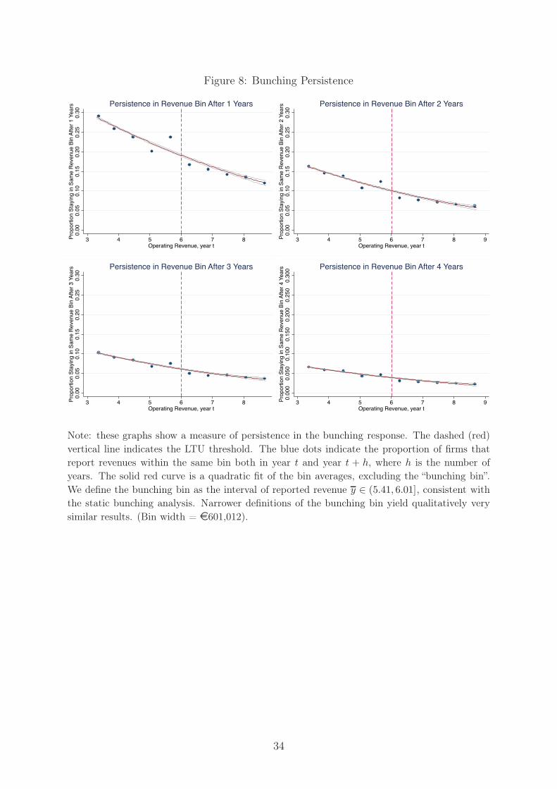
Figure 8: Bunching Persistence0.

000.

050.

100.

150.

200.

250.

30Pr

opor

tion

Stay

ing

in S

ame

Reve

nue

Bin

Afte

r 1 Y

ears

3 4 5 6 7 8 9Operating Revenue, year t

Persistence in Revenue Bin After 1 Years

0.00

0.05

0.10

0.15

0.20

0.25

0.30

Prop

ortio

n St

ayin

g in

Sam

e Re

venu

e Bi

n Af

ter 2

Yea

rs

3 4 5 6 7 8 9Operating Revenue, year t

Persistence in Revenue Bin After 2 Years

0.00

0.05

0.10

0.15

0.20

0.25

0.30

Prop

ortio

n St

ayin

g in

Sam

e Re

venu

e Bi

n Af

ter 3

Yea

rs

3 4 5 6 7 8 9Operating Revenue, year t

Persistence in Revenue Bin After 3 Years

0.00

00.

050

0.10

00.

150

0.20

00.

250

0.30

0Pr

opor

tion

Stay

ing

in S

ame

Reve

nue

Bin

Afte

r 4 Y

ears

3 4 5 6 7 8 9Operating Revenue, year t

Persistence in Revenue Bin After 4 Years

Note: these graphs show a measure of persistence in the bunching response. The dashed (red)

vertical line indicates the LTU threshold. The blue dots indicate the proportion of firms thatreport revenues within the same bin both in year t and year t + h, where h is the number ofyears. The solid red curve is a quadratic fit of the bin averages, excluding the “bunching bin”.

We define the bunching bin as the interval of reported revenue y ∈ (5.41, 6.01], consistent withthe static bunching analysis. Narrower definitions of the bunching bin yield qualitatively very

similar results. (Bin width = e601,012).

34

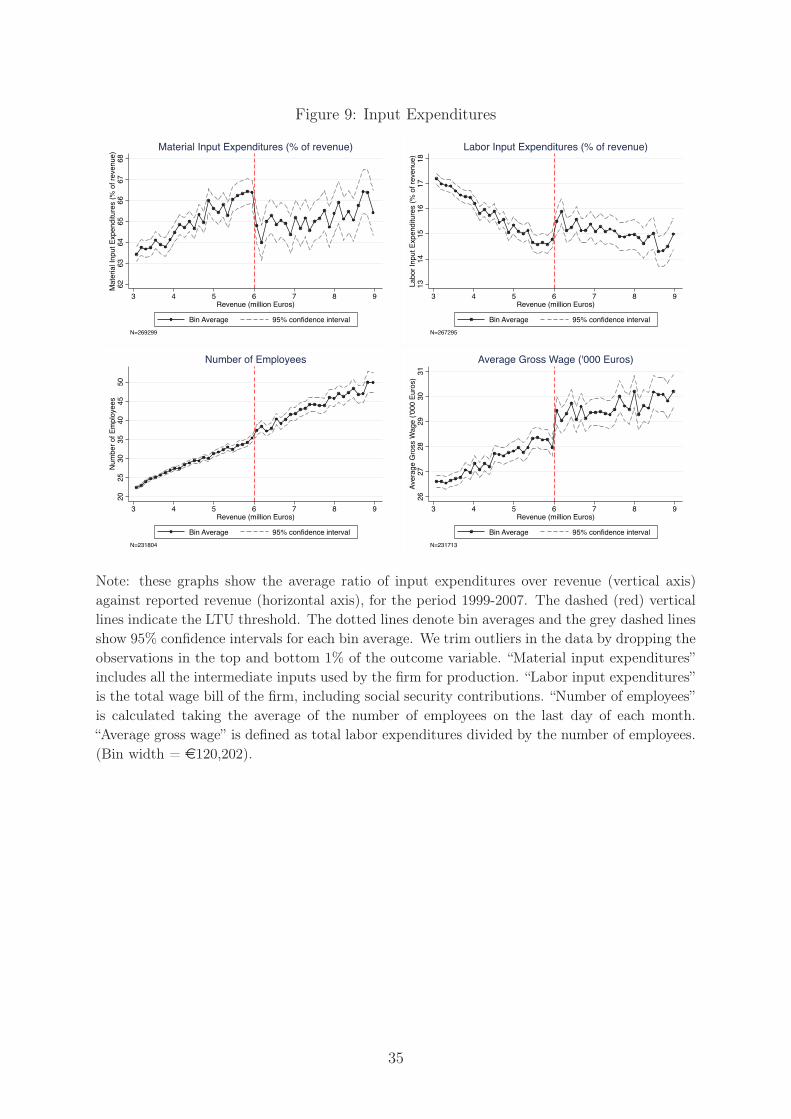
Figure 9: Input Expenditures62

6364

6566

6768

Mat

eria

l Inp

ut E

xpen

ditu

res

(% o

f rev

enue

)

3 4 5 6 7 8 9Revenue (million Euros)

Bin Average 95% confidence intervalN=269299

Material Input Expenditures (% of revenue)

1314

1516

1718

Labo

r Inp

ut E

xpen

ditu

res

(% o

f rev

enue

)

3 4 5 6 7 8 9Revenue (million Euros)

Bin Average 95% confidence intervalN=267295

Labor Input Expenditures (% of revenue)

2025

3035

4045

50N

umbe

r of E

mpl

oyee

s

3 4 5 6 7 8 9Revenue (million Euros)

Bin Average 95% confidence intervalN=231804

Number of Employees

2627

2829

3031

Aver

age

Gro

ss W

age

('000

Eur

os)

3 4 5 6 7 8 9Revenue (million Euros)

Bin Average 95% confidence intervalN=231713

Average Gross Wage ('000 Euros)

Note: these graphs show the average ratio of input expenditures over revenue (vertical axis)

against reported revenue (horizontal axis), for the period 1999-2007. The dashed (red) verticallines indicate the LTU threshold. The dotted lines denote bin averages and the grey dashed linesshow 95% confidence intervals for each bin average. We trim outliers in the data by dropping the

observations in the top and bottom 1% of the outcome variable. “Material input expenditures”includes all the intermediate inputs used by the firm for production. “Labor input expenditures”is the total wage bill of the firm, including social security contributions. “Number of employees”

is calculated taking the average of the number of employees on the last day of each month.“Average gross wage” is defined as total labor expenditures divided by the number of employees.

(Bin width = e120,202).

35

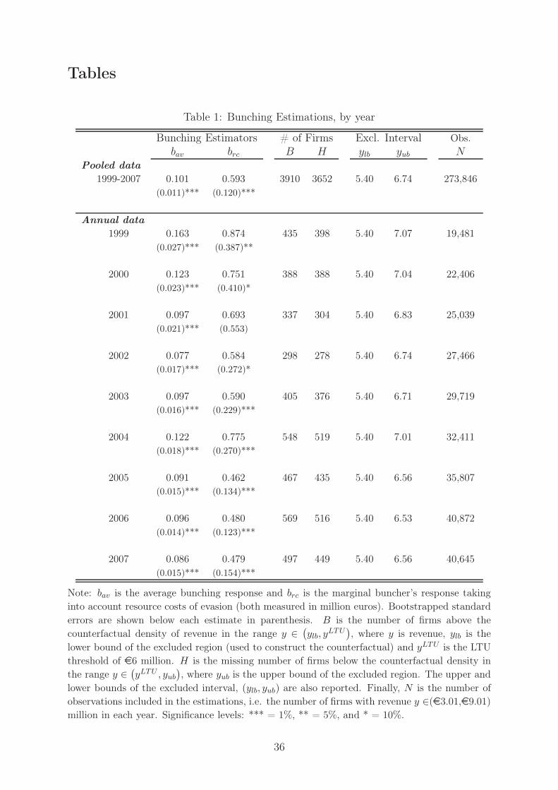
Tables

Table 1: Bunching Estimations, by year

Bunching Estimators # of Firms Excl. Interval Obs.

bav brc B H ylb yub NPooled data

1999-2007 0.101 0.593 3910 3652 5.40 6.74 273,846

(0.011)*** (0.120)***

Annual data

1999 0.163 0.874 435 398 5.40 7.07 19,481

(0.027)*** (0.387)**

2000 0.123 0.751 388 388 5.40 7.04 22,406

(0.023)*** (0.410)*

2001 0.097 0.693 337 304 5.40 6.83 25,039

(0.021)*** (0.553)

2002 0.077 0.584 298 278 5.40 6.74 27,466(0.017)*** (0.272)*

2003 0.097 0.590 405 376 5.40 6.71 29,719(0.016)*** (0.229)***

2004 0.122 0.775 548 519 5.40 7.01 32,411(0.018)*** (0.270)***

2005 0.091 0.462 467 435 5.40 6.56 35,807(0.015)*** (0.134)***

2006 0.096 0.480 569 516 5.40 6.53 40,872

(0.014)*** (0.123)***

2007 0.086 0.479 497 449 5.40 6.56 40,645

(0.015)*** (0.154)***

Note: bav is the average bunching response and brc is the marginal buncher’s response takinginto account resource costs of evasion (both measured in million euros). Bootstrapped standard

errors are shown below each estimate in parenthesis. B is the number of firms above thecounterfactual density of revenue in the range y ∈

"ylb, yLTU

#, where y is revenue, ylb is the

lower bound of the excluded region (used to construct the counterfactual) and yLTU is the LTUthreshold of e6 million. H is the missing number of firms below the counterfactual density inthe range y ∈

"yLTU , yub

#, where yub is the upper bound of the excluded region. The upper and

lower bounds of the excluded interval, (ylb, yub) are also reported. Finally, N is the number ofobservations included in the estimations, i.e. the number of firms with revenue y ∈(e3.01,e9.01)million in each year. Significance levels: *** = 1%, ** = 5%, and * = 10%.

36

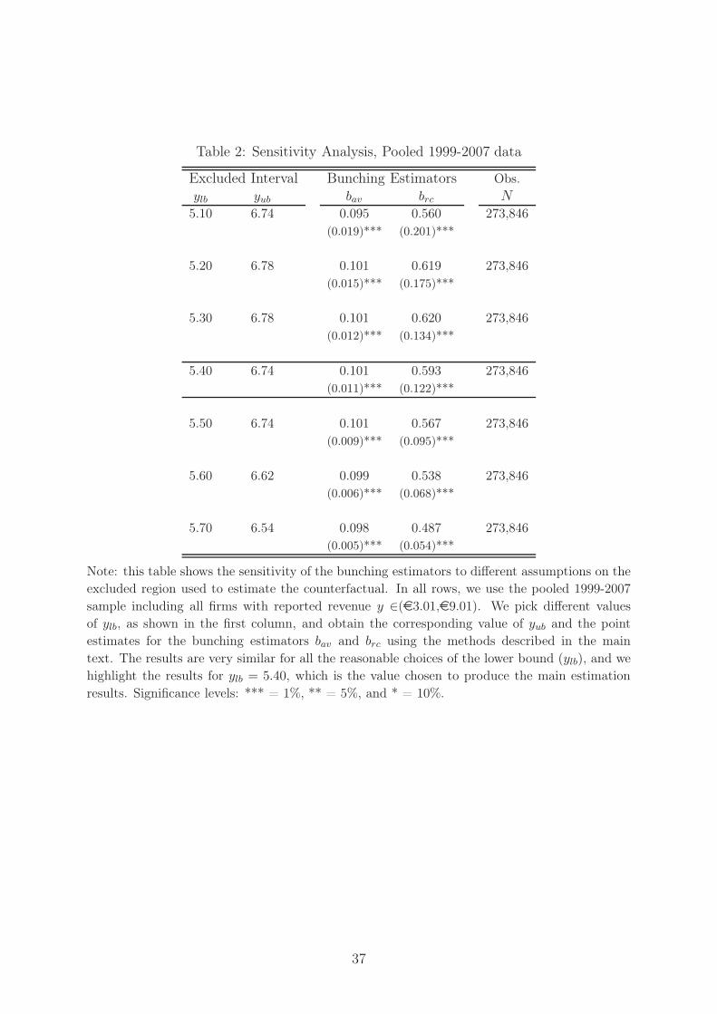
Table 2: Sensitivity Analysis, Pooled 1999-2007 data

Excluded Interval Bunching Estimators Obs.

ylb yub bav brc N5.10 6.74 0.095 0.560 273,846

(0.019)*** (0.201)***

5.20 6.78 0.101 0.619 273,846

(0.015)*** (0.175)***

5.30 6.78 0.101 0.620 273,846

(0.012)*** (0.134)***

5.40 6.74 0.101 0.593 273,846(0.011)*** (0.122)***

5.50 6.74 0.101 0.567 273,846

(0.009)*** (0.095)***

5.60 6.62 0.099 0.538 273,846(0.006)*** (0.068)***

5.70 6.54 0.098 0.487 273,846(0.005)*** (0.054)***

Note: this table shows the sensitivity of the bunching estimators to different assumptions on theexcluded region used to estimate the counterfactual. In all rows, we use the pooled 1999-2007

sample including all firms with reported revenue y ∈(e3.01,e9.01). We pick different valuesof ylb, as shown in the first column, and obtain the corresponding value of yub and the pointestimates for the bunching estimators bav and brc using the methods described in the main

text. The results are very similar for all the reasonable choices of the lower bound (ylb), and wehighlight the results for ylb = 5.40, which is the value chosen to produce the main estimation

results. Significance levels: *** = 1%, ** = 5%, and * = 10%.

37

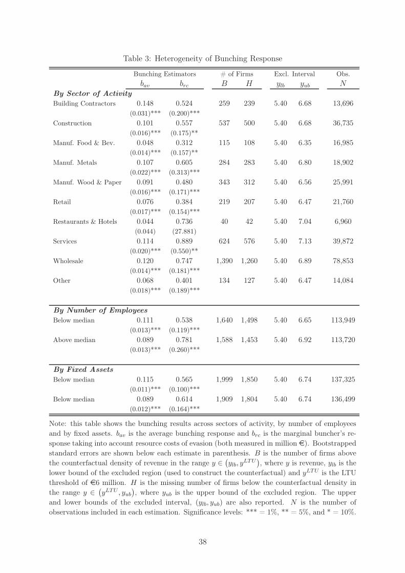
Table 3: Heterogeneity of Bunching Response

Bunching Estimators # of Firms Excl. Interval Obs.

bav brc B H ylb yub NBy Sector of Activity

Building Contractors 0.148 0.524 259 239 5.40 6.68 13,696

(0.031)*** (0.200)***

Construction 0.101 0.557 537 500 5.40 6.68 36,735

(0.016)*** (0.175)**

Manuf. Food & Bev. 0.048 0.312 115 108 5.40 6.35 16,985(0.014)*** (0.157)**

Manuf. Metals 0.107 0.605 284 283 5.40 6.80 18,902(0.022)*** (0.313)***

Manuf. Wood & Paper 0.091 0.480 343 312 5.40 6.56 25,991(0.016)*** (0.171)***

Retail 0.076 0.384 219 207 5.40 6.47 21,760

(0.017)*** (0.154)***

Restaurants & Hotels 0.044 0.736 40 42 5.40 7.04 6,960(0.044) (27.881)

Services 0.114 0.889 624 576 5.40 7.13 39,872(0.020)*** (0.550)**

Wholesale 0.120 0.747 1,390 1,260 5.40 6.89 78,853(0.014)*** (0.181)***

Other 0.068 0.401 134 127 5.40 6.47 14,084

(0.018)*** (0.189)***

By Number of Employees

Below median 0.111 0.538 1,640 1,498 5.40 6.65 113,949

(0.013)*** (0.119)***

Above median 0.089 0.781 1,588 1,453 5.40 6.92 113,720(0.013)*** (0.260)***

By Fixed Assets

Below median 0.115 0.565 1,999 1,850 5.40 6.74 137,325(0.011)*** (0.100)***

Below median 0.089 0.614 1,909 1,804 5.40 6.74 136,499(0.012)*** (0.164)***

Note: this table shows the bunching results across sectors of activity, by number of employeesand by fixed assets. bav is the average bunching response and brc is the marginal buncher’s re-

sponse taking into account resource costs of evasion (both measured in million e). Bootstrappedstandard errors are shown below each estimate in parenthesis. B is the number of firms abovethe counterfactual density of revenue in the range y ∈

"ylb, yLTU

#, where y is revenue, ylb is the

lower bound of the excluded region (used to construct the counterfactual) and yLTU is the LTUthreshold of e6 million. H is the missing number of firms below the counterfactual density inthe range y ∈

"yLTU , yub

#, where yub is the upper bound of the excluded region. The upper

and lower bounds of the excluded interval, (ylb, yub) are also reported. N is the number ofobservations included in each estimation. Significance levels: *** = 1%, ** = 5%, and * = 10%.

38

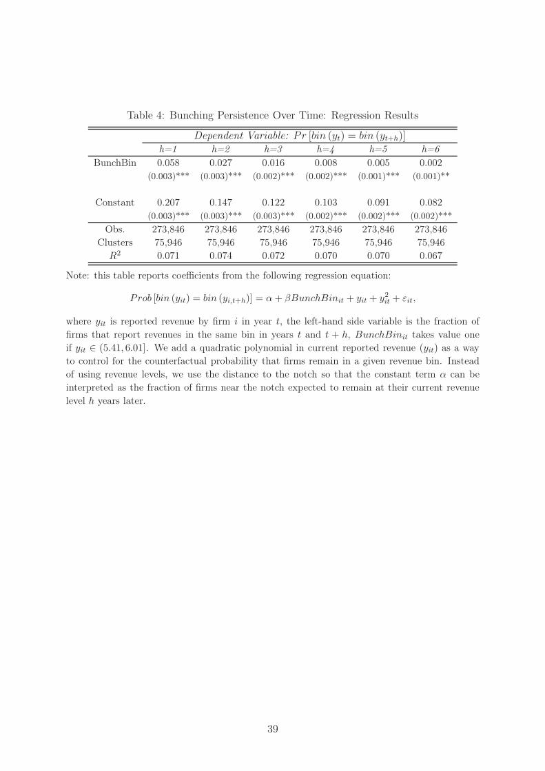
Table 4: Bunching Persistence Over Time: Regression Results

Dependent Variable: Pr [bin (yt) = bin (yt+h)]h=1 h=2 h=3 h=4 h=5 h=6

BunchBin 0.058 0.027 0.016 0.008 0.005 0.002(0.003)*** (0.003)*** (0.002)*** (0.002)*** (0.001)*** (0.001)**

Constant 0.207 0.147 0.122 0.103 0.091 0.082(0.003)*** (0.003)*** (0.003)*** (0.002)*** (0.002)*** (0.002)***

Obs. 273,846 273,846 273,846 273,846 273,846 273,846Clusters 75,946 75,946 75,946 75,946 75,946 75,946

R2 0.071 0.074 0.072 0.070 0.070 0.067

Note: this table reports coefficients from the following regression equation:

Prob [bin (yit) = bin (yi,t+h)] = α+ βBunchBinit + yit + y2it + εit,

where yit is reported revenue by firm i in year t, the left-hand side variable is the fraction of

firms that report revenues in the same bin in years t and t + h, BunchBinit takes value oneif yit ∈ (5.41, 6.01]. We add a quadratic polynomial in current reported revenue (yit) as a wayto control for the counterfactual probability that firms remain in a given revenue bin. Instead

of using revenue levels, we use the distance to the notch so that the constant term α can beinterpreted as the fraction of firms near the notch expected to remain at their current revenue

level h years later.

39

Online Appendix

Not Intended for Publication

“Heterogeneous Responses to Effective TaxEnforcement: Evidence from Spanish Firms”

by Miguel Almunia (Warwick) and David Lopez-Rodriguez(Banco de España)

40

A Data: Further Details

Definition of Sectors of Activity

The table below provides the 2- or 3-digit codes from the North-American Industry

Classification System (NAICS, 2002) that we use to define sectors of activity in the

empirical estimation. The middle column shows the number of firms in each sector for

the pooled 1999-2007 dataset, and the percentage they represent overall.

Sector NAICS-2002 Codes # of Firms

Construction 236 - Construction of buildings 36,735 (13.2%)

Building Contractors 238 - Specialty trade contractors 13,696 (5.0%)

Manufacturing 31 - Food and beverage products 16,985 (6.2%)

32 - Wood, paper, chemical products 25,991 (9.5%)

33 - Metal products, machinery 18,902 (6.9%)

Wholesale 42 - Wholesale trade 78,853 (28.8%)

Retail 44 & 45 - Retail trade 21,760 (8.0%)

Restaurants & Hotels 72 - Restaurants and hotels 6,960 (2.5%)

Services 48 - Transportation 54 - Professional services 39,872 (14.6%)

49 - Postal & warehousing 55 - Management of firms

51 - Information 56 - Administrative support

52 - Finance and insurance 81 - Other services

53 - Real estate

Other 11 - Agriculture & fishing 61 - Education services 14,084 (5.1%)

21 - Mining 62 - Health services

22 - Utility companies 71 - Arts and entertainment

237 - Civil engineering 92 - Public administration

Source: www.census.gov/cgi-bin/sssd/naics/naicsrch?chart=2002

41

Amadeus data and Final dataset

To build the final dataset for this paper, we proceed as follows. In December 2011, we

downloaded all the data available for Spanish firms in Amadeus, accessed online through

Wharton Research Data Services (WRDS). This dataset is updated monthly and firms

that have not reported information for 4 consecutive years are dropped, so it is possible

that a subset firms that are included in our analysis are no longer in the online version

of Amadeus. We include data for the years 1999 through 2007, both included.

In order to construct our final dataset for analysis, we take several steps. First, we

drop observations from two regions where tax collection is independent of the federal tax

authority and hence the LTU threshold does not apply (Pais Vasco and Navarra). Second,

we choose a bin width of e60,101, which is one-hundredth of the revenue level of the LTU

threshold. For symmetry, we keep 50 bins below and 50 bins above the threshold, so in

total there are 100 bins. Hence, our final dataset has firms with reported revenue between

e3.005 million and e9.015 million. Within this range, we define some of the ratios that

we use in the section on input expenditures: materials and labor expenditures as % of

revenue, average gross wages (defined as the total wage bill divided by the number of

employees), and fixed assets as % of revenue. Finally, we drop the top and bottom 1%

of observations from each of these variables, in order to avoid the presence of outliers in

the data. There is some overlap in the extreme values, such that a firm with abnormally

high materials is likely to have abnormally low labor expenditures. The final dataset

contains 273,846 observations, and summary statistics are reported on Table A.1. The

Stata do-files used to process the original data to arrive at the final dataset are available

upon request.

Input-Output Tables

We use the input-output tables produced by the National Statistics Institute (Instituto

Nacional de Estadística, INE ) for the year 2000. Sectors of activity are defined according

to Spanish industry classification, which does not match NAICS codes exactly but has

substantial overlap. To calculate the share of sales made to final consumers by sector, we

divide the column labelled “Consumo final de los hogares, interno” (“Households’ final

consumption, domestic”) by the column “Total empleos” (“Total uses”). The original table

used for the calculations can be downloaded from:

www.ine.es/daco/daco42/cne00/simetrica2000.xls

The table we provide together with our main dataset contains, additionally, the cor-

respondence between our sector definitions (based on NAICS 2002 codes) and the sectors

defined in the input-output tables.

42

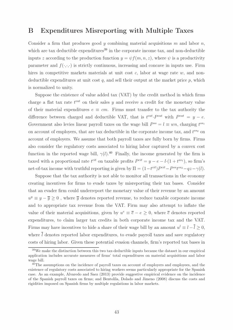
B Expenditures Misreporting with Multiple Taxes

Consider a firm that produces good y combining material acquisitions m and labor n,

which are tax deductible expenditures39 in the corporate income tax, and non-deductible

inputs z according to the production function y = ψf(m,n, z), where ψ is a productivity

parameter and f(·,·,·) is strictly continuous, increasing and concave in inputs use. Firm

hires in competitive markets materials at unit cost c, labor at wage rate w, and non-

deductible expenditures at unit cost q, and sell their output at the market price p, which

is normalized to unity.

Suppose the existence of value added tax (VAT) by the credit method in which firms

charge a flat tax rate tvat on their sales y and receive a credit for the monetary value

of their material expenditures e ≡ cm. Firms must transfer to the tax authority the

difference between charged and deductible VAT, that is tvat·P vat with P vat = y − e.

Government also levies linear payroll taxes on the wage bill P ss = l ≡ wn, charging tss1

on account of employers, that are tax deductible in the corporate income tax, and tss2 on

account of employers. We assume that both payroll taxes are fully born by firms. Firms

also consider the regulatory costs associated to hiring labor captured by a convex cost

function in the reported wage bill, γ(l).40 Finally, the income generated by the firm is

taxed with a proportional rate tcit on taxable profits P cit = y − e− l·(1 + tss1), so firm’s

net-of-tax income with truthful reporting is given by Π = (1−tcit)P cit−P sstss2−qz−γ(l).

Suppose that the tax authority is not able to monitor all transactions in the economy

creating incentives for firms to evade taxes by misreporting their tax bases. Consider

that an evader firm could underreport the monetary value of their revenue by an amount

uy ≡ y − y ≥ 0 , where y denotes reported revenue, to reduce taxable corporate income

and to appropriate tax revenue from the VAT. Firm may also attempt to inflate the

value of their material acquisitions, given by ue ≡ e − e ≥ 0, where e denotes reported

expenditures, to claim larger tax credits in both corporate income tax and the VAT.

Firms may have incentives to hide a share of their wage bill by an amount ul ≡ l− l ≥ 0,

where l denotes reported labor expenditures, to evade payroll taxes and save regulatory

costs of hiring labor. Given these potential evasion channels, firm’s reported tax bases in

39We make the distinction between this two tax-deductible inputs because the dataset in our empiricalapplication includes accurate measures of firms’ total expenditures on material acquisitions and laborwage bill.

40The assumptions on the incidence of payroll taxes on account of employers and employees, and theexistence of regulatory costs associated to hiring workers seems particularly appropriate for the Spanishcase. As an example, Alvaredo and Saez (2013) provide suggestive empirical evidence on the incidenceof the Spanish payroll taxes on firms; and Bentolila, Dolado and Jimeno (2008) discuss the costs andrigidities imposed on Spanish firms by multiple regulations in labor markets.

43

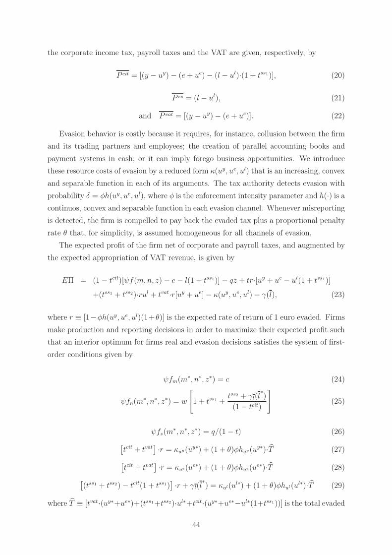
the corporate income tax, payroll taxes and the VAT are given, respectively, by

P cit = [(y − uy)− (e+ ue)− (l − ul)·(1 + tss1)], (20)

P ss = (l − ul), (21)

and P vat = [(y − uy)− (e+ ue)]. (22)

Evasion behavior is costly because it requires, for instance, collusion between the firm

and its trading partners and employees; the creation of parallel accounting books and

payment systems in cash; or it can imply forego business opportunities. We introduce

these resource costs of evasion by a reduced form κ(uy, ue, ul) that is an increasing, convex

and separable function in each of its arguments. The tax authority detects evasion with

probability δ = φh(uy, ue, ul), where φ is the enforcement intensity parameter and h(·) is a

continuos, convex and separable function in each evasion channel. Whenever misreporting

is detected, the firm is compelled to pay back the evaded tax plus a proportional penalty

rate θ that, for simplicity, is assumed homogeneous for all channels of evasion.

The expected profit of the firm net of corporate and payroll taxes, and augmented by

the expected appropriation of VAT revenue, is given by

EΠ = (1− tcit)[ψf(m,n, z)− e− l(1 + tss1)]− qz + tr·[uy + ue − ul(1 + tss1)]

+(tss1 + tss2)·rul + tvat·r[uy + ue]− κ(uy, ue, ul)− γ(l), (23)

where r ≡ [1−φh(uy, ue, ul)(1+θ)] is the expected rate of return of 1 euro evaded. Firms

make production and reporting decisions in order to maximize their expected profit such

that an interior optimum for firms real and evasion decisions satisfies the system of first-

order conditions given by

ψfm(m∗, n∗, z∗) = c (24)

ψfn(m∗, n∗, z∗) = w

.

1 + tss1 +tss2 + γl(l

∗

)

(1− tcit)

/

(25)

ψfz(m∗, n∗, z∗) = q/(1− t) (26)

!tcit + tvat

$·r = κuy(uy∗) + (1 + θ)φhuy(uy∗)·(T (27)

!tcit + tvat

$·r = κue(ue∗) + (1 + θ)φhue(ue∗)·(T (28)

!(tss1 + tss2)− tcit(1 + tss1)

$·r + γl(l

∗

) = κul(ul∗) + (1 + θ)φhul(ul∗)·(T (29)

where (T ≡ [tvat·(uy∗+ue∗)+(tss1+tss2)·ul∗+tcit·(uy∗+ue∗−ul∗(1+tss1))] is the total evaded

44

taxes by the multiple misreporting channels. The system of optimal conditions shows that

positive tax rates on corporate income distort inputs demand decisions reducing revenue

from potential production at zero tax rates. These conditions also indicate that the

existence of both payroll taxes and labor regulatory costs create distortions increasing

the marginal cost of hiring employees and thus reducing labor demand.

The optimal evasion conditions for each misreporting channel predict that firm evades

taxes to the point where the marginal expected return of misreporting transactions is

equal to the expected costs associated to tax evasion. The latter is the result of the

marginal resource costs born in each misreporting channel plus the deterrence effect cre-

ated by tax enforcement that results from the interaction between monitoring effort and

the existence of paper trail. The systematic matching of tax returns from multiple tax-

payers implies that a marginal unit of misreporting in one channel increases the chances

of being detected, and thus paying back the total amount evaded, in multiple channels.

The expected returns of misreporting revenue and expenditures are positively related

with the tax rates. The larger the tax rates on both the VAT and the corporate income tax

are, the higher the incentives to hide revenue and inflate material acquisitions to reduce

those tax bases. Notice that when firms have scope to misreport their transactions they

do not act as fiscal intermediaries, that just transfer collected VAT to the tax agency, but

instead firms have incentives to appropriate a share of VAT revenue. Finally, the optimal

condition for hidden labor bill indicates that firms could have incentives to misreport

it when the marginal savings in payroll taxes and regulatory costs were larger than the

foregoing tax credits in corporate income tax due misreporting of labor costs. Overall,

the model identifies two channels that create positive returns for labor misreporting: i)

the existence of a significant gap between payroll taxes and corporate tax rates; and ii)

the presence of large regulatory costs associated to hiring workers.

B.1 Anatomy of the Response: Input Ratios at the LTU Thresh-

old

Consider the extended model with heterogeneous enforcement intensities and resource

costs presented in section 2. Before the introduction of a LTU, the system of optimal

conditions indicates that the demand of tax-deductible inputs (e.g. materials and labor)

is smoothly increasing in productivity, dm/dψ > 0 and dn/dψ > 0. Hence, the reported

ratios of input expenditures over revenue, M ≡ cm/y and L ≡ wn/y, are continuous in

ψ over the range [ψ,ψ]. This implies that in the neighborhood of yL defined by the small

interval (y′, yL + dyMφ ) the average reported ratios of inputs expenditures over revenue

45

are almost equal, that is,

´ yL

y′ M ·g0(y)dy´ yL

y′ g0(y)dy∼=

´ yL+dyMφyL M ·g0(y)dy´ yL+dyMφyL g0(y)dy

and

´ yL

y′ L·g0(y)dy´ yL

y′ g0(y)dy∼=

´ yL+dyMφyL L·g0(y)dy´ yL+dyMφyL g0(y)dy

.

(30)

Suppose the LTU is introduced. In the presence of resource costs we assume that

there is a constant proportion of firms α with prohibitive resource costs to react in the

pre-LTU density interval (defined) by (yL, yL + dyMφ ) . In contrast, there is a proportion

1 − α of firms in this interval, the bunchers, that reduce their reported revenue to stay

below the threshold when that results in larger expected profits, i.e. EΠ0(m,n, z, u |

ψM ,φ0) > EΠ1(m,n, z, u | ψM ,φ1). Assuming that the bunchers locate in the interval

(y′, yL), we obtain different predictions on the expected average reported ratios of input

expenditures over revenue around the LTU threshold depending on whether these firms’

reaction is due real (i.e. reduction of production) or evasion (i.e. increase of concealed

revenue) adjustments.41

Real Response. Bunchers can react to the threshold lowering their production, and

thus their inputs demand, without bearing additional resource costs of evasion. This

reaction yields that in the interval (y′, yL) below the threshold there are firms with ψ ∈

[ψ′,ψL] that hire more inputs than bunchers with ψ ∈ [ψL,ψM ]. This causes that both

average reported ratios of expenditures over revenue are not continuous at the threshold

yL. The reaction of the bunchers to the LTU yields a (discrete) upward jump of these

ratios at the threshold such that

´ yL

y′ M ·g1(y)dy´ yL

y′ g1(y)dy<

´ yL+dyMφyL M ·g1(y)dy´ yL+dyM

φ

yL g1(y)dyand

´ yL

y′ L·g1(y)dy´ yL

y′ g1(y)dy<

´ yL+dyMφyL L·g1(y)dy´ yL+dyM

φ

yL g1(y)dy.

(31)

Evasion Response. Bunchers can react to the threshold increasing their concealed

revenue, and thus without modifying their inputs demand, paying resource costs of ad-

ditional evasion. This response implies that in the interval (y′, yL) below the threshold

firms with ψ ∈ [ψ′,ψL] hire lower inputs than bunchers with ψ ∈ [ψL,ψM ]. The response

of the bunchers thus creates a discontinuity in the average reported ratios of expenditures

at the threshold yL with a (discrete) downward jump of these ratios at the threshold such

41The bunchers’ reaction to the LTU threshold could be a combination of both potential responses,real and evasion, but we discuss the two polar responses for analytical simplicity. This simplificationprovides predictions on the expected average patterns of input ratios around the threshold when thereaction is dominated by either the real or the evasion channel.

46

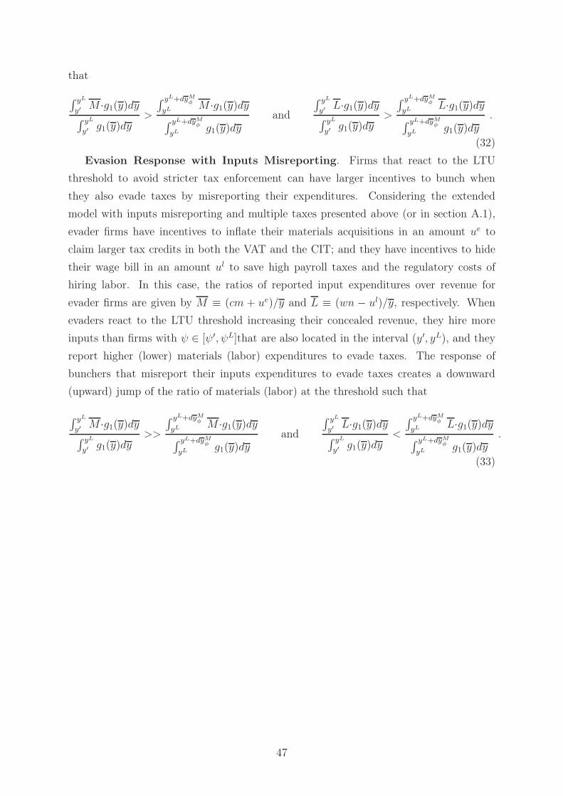
that

´ yL

y′ M ·g1(y)dy´ yL

y′ g1(y)dy>

´ yL+dyMφyL M ·g1(y)dy´ yL+dyM

φ

yL g1(y)dyand

´ yL

y′ L·g1(y)dy´ yL

y′ g1(y)dy>

´ yL+dyMφyL L·g1(y)dy´ yL+dyM

φ

yL g1(y)dy.

(32)

Evasion Response with Inputs Misreporting. Firms that react to the LTU

threshold to avoid stricter tax enforcement can have larger incentives to bunch when

they also evade taxes by misreporting their expenditures. Considering the extended

model with inputs misreporting and multiple taxes presented above (or in section A.1),

evader firms have incentives to inflate their materials acquisitions in an amount ue to

claim larger tax credits in both the VAT and the CIT; and they have incentives to hide

their wage bill in an amount ul to save high payroll taxes and the regulatory costs of

hiring labor. In this case, the ratios of reported input expenditures over revenue for

evader firms are given by M ≡ (cm + ue)/y and L ≡ (wn − ul)/y, respectively. When

evaders react to the LTU threshold increasing their concealed revenue, they hire more

inputs than firms with ψ ∈ [ψ′,ψL]that are also located in the interval (y′, yL), and they

report higher (lower) materials (labor) expenditures to evade taxes. The response of

bunchers that misreport their inputs expenditures to evade taxes creates a downward

(upward) jump of the ratio of materials (labor) at the threshold such that

´ yL

y′ M ·g1(y)dy´ yL

y′ g1(y)dy>>

´ yL+dyMφyL M ·g1(y)dy´ yL+dyM

φ

yL g1(y)dyand

´ yL

y′ L·g1(y)dy´ yL

y′ g1(y)dy<

´ yL+dyMφyL L·g1(y)dy´ yL+dyM

φ

yL g1(y)dy.

(33)

47

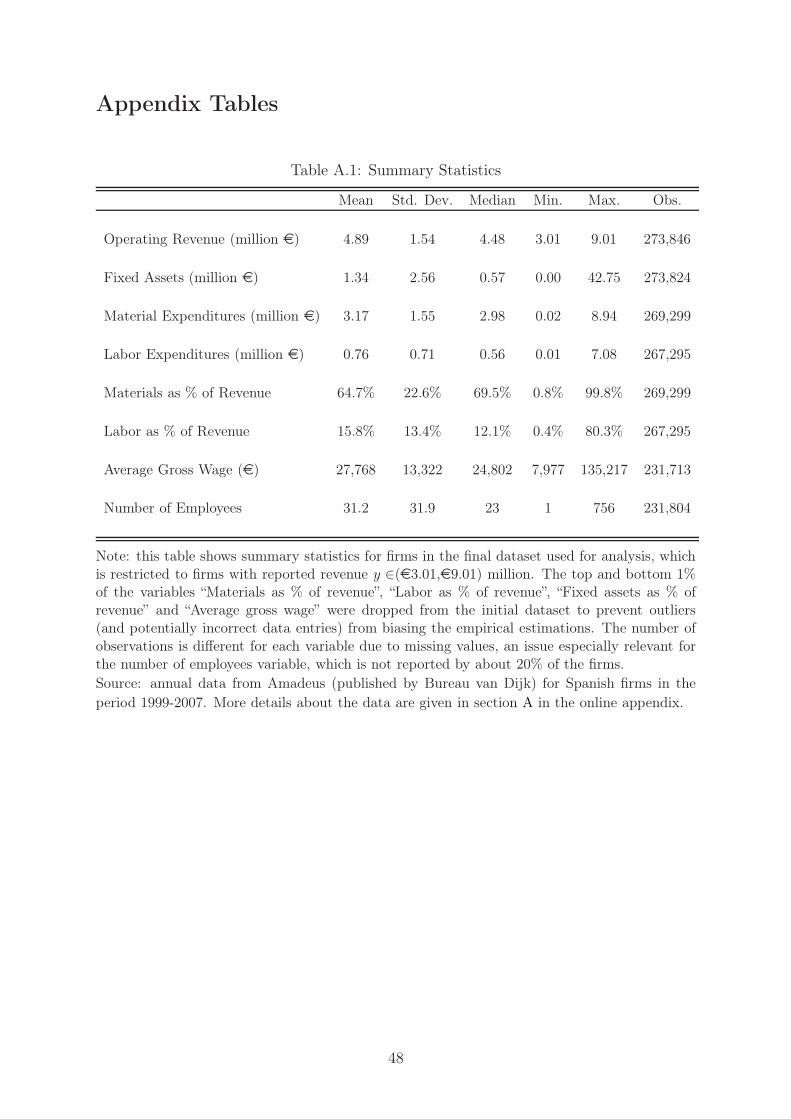
Appendix Tables

Table A.1: Summary Statistics

Mean Std. Dev. Median Min. Max. Obs.

Operating Revenue (million e) 4.89 1.54 4.48 3.01 9.01 273,846

Fixed Assets (million e) 1.34 2.56 0.57 0.00 42.75 273,824

Material Expenditures (million e) 3.17 1.55 2.98 0.02 8.94 269,299

Labor Expenditures (million e) 0.76 0.71 0.56 0.01 7.08 267,295

Materials as % of Revenue 64.7% 22.6% 69.5% 0.8% 99.8% 269,299

Labor as % of Revenue 15.8% 13.4% 12.1% 0.4% 80.3% 267,295

Average Gross Wage (e) 27,768 13,322 24,802 7,977 135,217 231,713

Number of Employees 31.2 31.9 23 1 756 231,804

Note: this table shows summary statistics for firms in the final dataset used for analysis, whichis restricted to firms with reported revenue y ∈(e3.01,e9.01) million. The top and bottom 1%of the variables “Materials as % of revenue”, “Labor as % of revenue”, “Fixed assets as % ofrevenue” and “Average gross wage” were dropped from the initial dataset to prevent outliers(and potentially incorrect data entries) from biasing the empirical estimations. The number ofobservations is different for each variable due to missing values, an issue especially relevant forthe number of employees variable, which is not reported by about 20% of the firms.Source: annual data from Amadeus (published by Bureau van Dijk) for Spanish firms in the

period 1999-2007. More details about the data are given in section A in the online appendix.

48

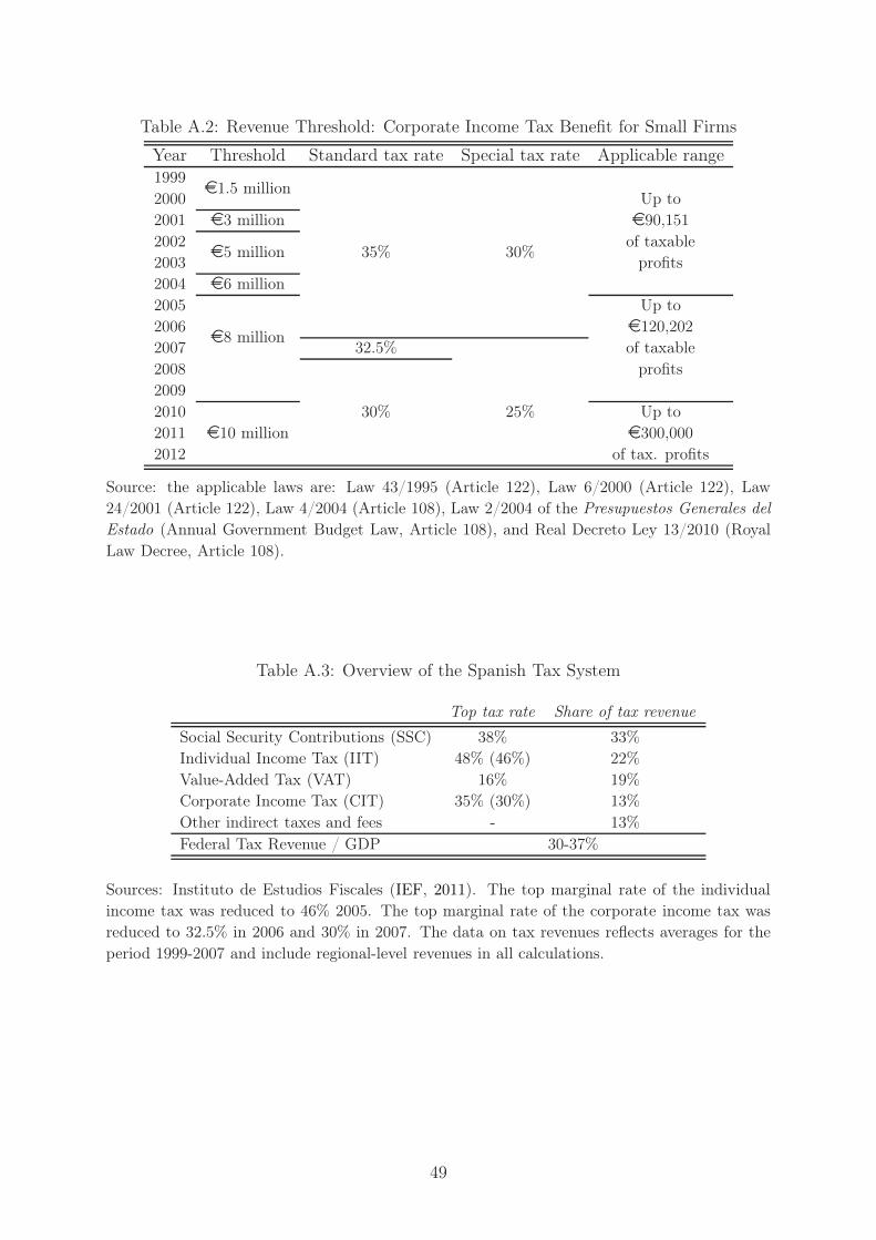
Table A.2: Revenue Threshold: Corporate Income Tax Benefit for Small Firms

Year Threshold Standard tax rate Special tax rate Applicable range1999

e1.5 million

35% 30%

2000 Up to2001 e3 million e90,151

2002e5 million

of taxable2003 profits2004 e6 million

2005

e8 million

Up to2006 e120,2022007 32.5% of taxable

2008

30% 25%

profits2009

2010e10 million

Up to2011 e300,0002012 of tax. profits

Source: the applicable laws are: Law 43/1995 (Article 122), Law 6/2000 (Article 122), Law24/2001 (Article 122), Law 4/2004 (Article 108), Law 2/2004 of the Presupuestos Generales del

Estado (Annual Government Budget Law, Article 108), and Real Decreto Ley 13/2010 (Royal

Law Decree, Article 108).

Table A.3: Overview of the Spanish Tax System

Top tax rate Share of tax revenue

Social Security Contributions (SSC) 38% 33%Individual Income Tax (IIT) 48% (46%) 22%

Value-Added Tax (VAT) 16% 19%Corporate Income Tax (CIT) 35% (30%) 13%

Other indirect taxes and fees - 13%

Federal Tax Revenue / GDP 30-37%

Sources: Instituto de Estudios Fiscales (IEF, 2011). The top marginal rate of the individualincome tax was reduced to 46% 2005. The top marginal rate of the corporate income tax wasreduced to 32.5% in 2006 and 30% in 2007. The data on tax revenues reflects averages for the

period 1999-2007 and include regional-level revenues in all calculations.

49

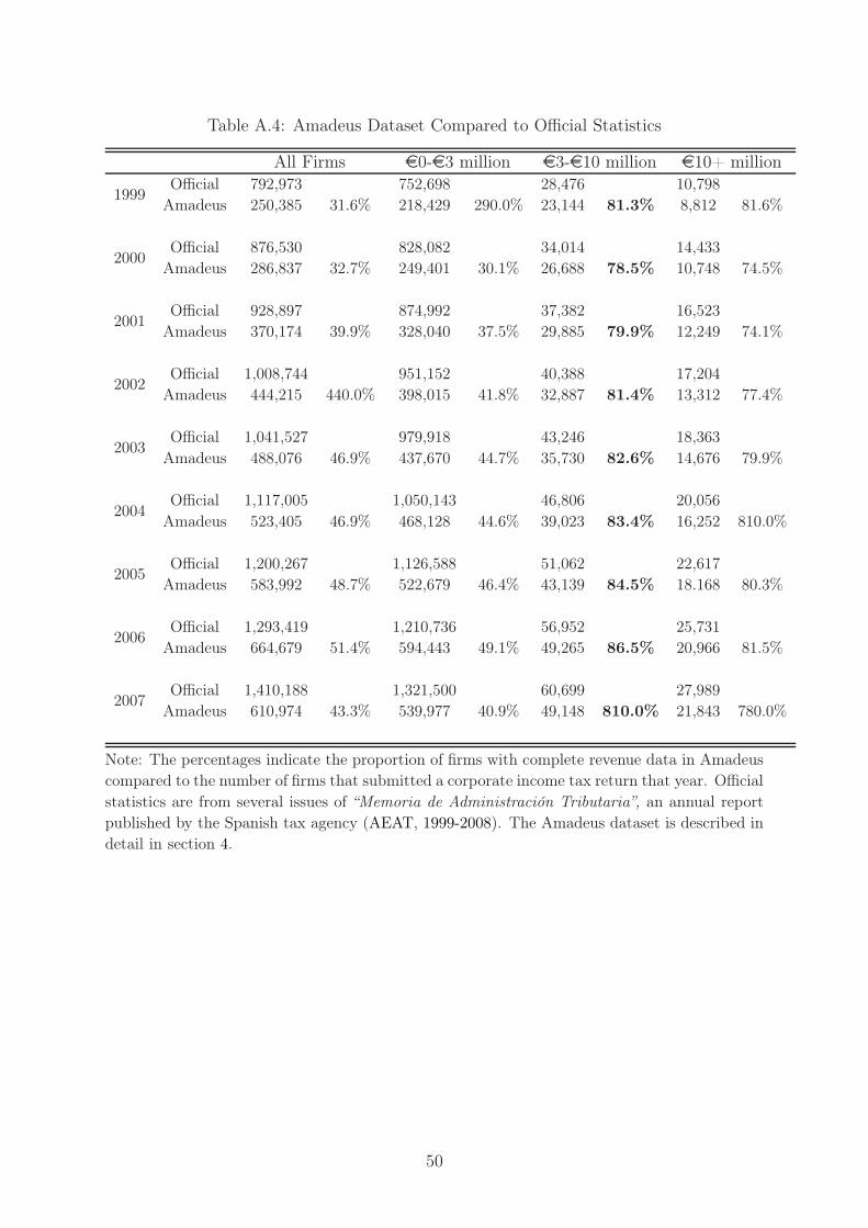
Table A.4: Amadeus Dataset Compared to Official Statistics

All Firms e0-e3 million e3-e10 million e10+ million

1999Official 792,973 752,698 28,476 10,798

Amadeus 250,385 31.6% 218,429 290.0% 23,144 81.3% 8,812 81.6%

2000Official 876,530 828,082 34,014 14,433

Amadeus 286,837 32.7% 249,401 30.1% 26,688 78.5% 10,748 74.5%

2001Official 928,897 874,992 37,382 16,523

Amadeus 370,174 39.9% 328,040 37.5% 29,885 79.9% 12,249 74.1%

2002Official 1,008,744 951,152 40,388 17,204

Amadeus 444,215 440.0% 398,015 41.8% 32,887 81.4% 13,312 77.4%

2003Official 1,041,527 979,918 43,246 18,363

Amadeus 488,076 46.9% 437,670 44.7% 35,730 82.6% 14,676 79.9%

2004Official 1,117,005 1,050,143 46,806 20,056

Amadeus 523,405 46.9% 468,128 44.6% 39,023 83.4% 16,252 810.0%

2005Official 1,200,267 1,126,588 51,062 22,617

Amadeus 583,992 48.7% 522,679 46.4% 43,139 84.5% 18.168 80.3%

2006Official 1,293,419 1,210,736 56,952 25,731

Amadeus 664,679 51.4% 594,443 49.1% 49,265 86.5% 20,966 81.5%

2007Official 1,410,188 1,321,500 60,699 27,989

Amadeus 610,974 43.3% 539,977 40.9% 49,148 810.0% 21,843 780.0%

Note: The percentages indicate the proportion of firms with complete revenue data in Amadeuscompared to the number of firms that submitted a corporate income tax return that year. Official

statistics are from several issues of “Memoria de Administración Tributaria”, an annual reportpublished by the Spanish tax agency (AEAT, 1999-2008). The Amadeus dataset is described indetail in section 4.

50

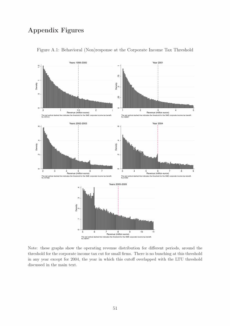
Appendix Figures

Figure A.1: Behavioral (Non)response at the Corporate Income Tax Threshold

0.5

11.

5D

ensi

ty

.5 1 1.5 2 2.5Revenue (million euros)

The red vertical dashed line indicates the threshold for the SME corporate income tax benefit.N=197313

Years 1999-2000

0.2

5.5

.75

1D

ensi

ty

1 2 3 4 5Revenue (million euros)

The red vertical dashed line indicates the threshold for the SME corporate income tax benefit.N=158607

Year 2001

0.2

.4.6

Den

sity

2 3 4 5 6 7 8Revenue (million euros)

The red vertical dashed line indicates the threshold for the SME corporate income tax benefit.N=107058

Years 2002-2003

0.2

.4.6

Den

sity

3 4 5 6 7 8 9Revenue (million euros)

The red vertical dashed line indicates the threshold for the SME corporate income tax benefit.N=37290

Year 2004

0.1

.2.3

.4D

ensi

ty

5 6 7 8 9 10 11Revenue (million euros)

The red vertical dashed line indicates the threshold for the SME corporate income tax benefit.N=100441

Years 2005-2009

Note: these graphs show the operating revenue distribution for different periods, around the

threshold for the corporate income tax cut for small firms. There is no bunching at this thresholdin any year except for 2004, the year in which this cutoff overlapped with the LTU thresholddiscussed in the main text.

51

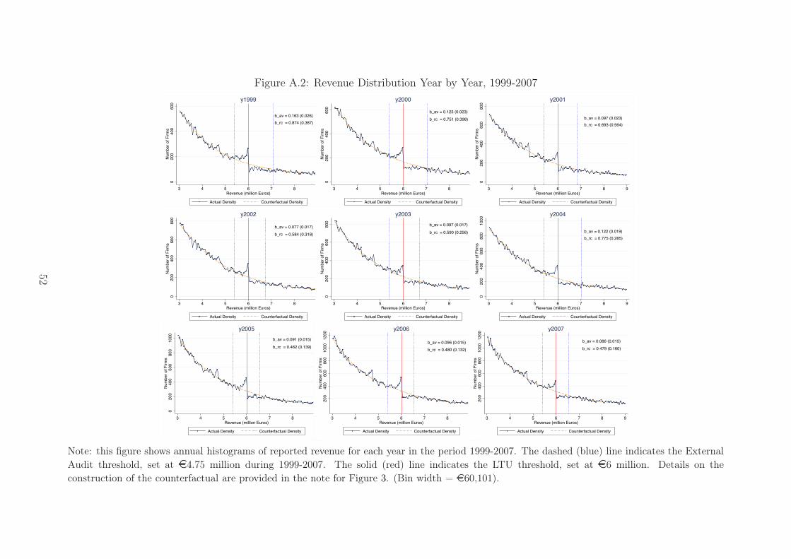
Figure A.2: Revenue Distribution Year by Year, 1999-2007

b_av = 0.163 (0.026)b_rc = 0.874 (0.387)

020

040

060

0N

umbe

r of F

irms

3 4 5 6 7 8 9Revenue (million Euros)

Actual Density Counterfactual Density

y1999

b_av = 0.123 (0.023)b_rc = 0.751 (0.398)

020

040

060

0N

umbe

r of F

irms

3 4 5 6 7 8 9Revenue (million Euros)

Actual Density Counterfactual Density

y2000

b_av = 0.097 (0.023)b_rc = 0.693 (0.564)

020

040

060

080

0N

umbe

r of F

irms

3 4 5 6 7 8 9Revenue (million Euros)

Actual Density Counterfactual Density

y2001

b_av = 0.077 (0.017)b_rc = 0.584 (0.318)

020

040

060

080

0N

umbe

r of F

irms

3 4 5 6 7 8 9Revenue (million Euros)

Actual Density Counterfactual Density

y2002b_av = 0.097 (0.017)

b_rc = 0.590 (0.256)

020

040

060

080

0N

umbe

r of F

irms

3 4 5 6 7 8 9Revenue (million Euros)

Actual Density Counterfactual Density

y2003

b_av = 0.122 (0.019)b_rc = 0.775 (0.285)

020

040

060

080

010

00N

umbe

r of F

irms

3 4 5 6 7 8 9Revenue (million Euros)

Actual Density Counterfactual Density

y2004

b_av = 0.091 (0.015)

b_rc = 0.462 (0.139)

020

040

060

080

010

00N

umbe

r of F

irms

3 4 5 6 7 8 9Revenue (million Euros)

Actual Density Counterfactual Density

y2005

b_av = 0.096 (0.015)b_rc = 0.480 (0.132)

200

400

600

800

1000

1200

Num

ber o

f Firm

s

3 4 5 6 7 8 9Revenue (million Euros)

Actual Density Counterfactual Density

y2006

b_av = 0.086 (0.015)b_rc = 0.479 (0.160)

200

400

600

800

1000

1200

Num

ber o

f Firm

s

3 4 5 6 7 8 9Revenue (million Euros)

Actual Density Counterfactual Density

y2007

Note: this figure shows annual histograms of reported revenue for each year in the period 1999-2007. The dashed (blue) line indicates the ExternalAudit threshold, set at e4.75 million during 1999-2007. The solid (red) line indicates the LTU threshold, set at e6 million. Details on theconstruction of the counterfactual are provided in the note for Figure 3. (Bin width = e60,101).

52

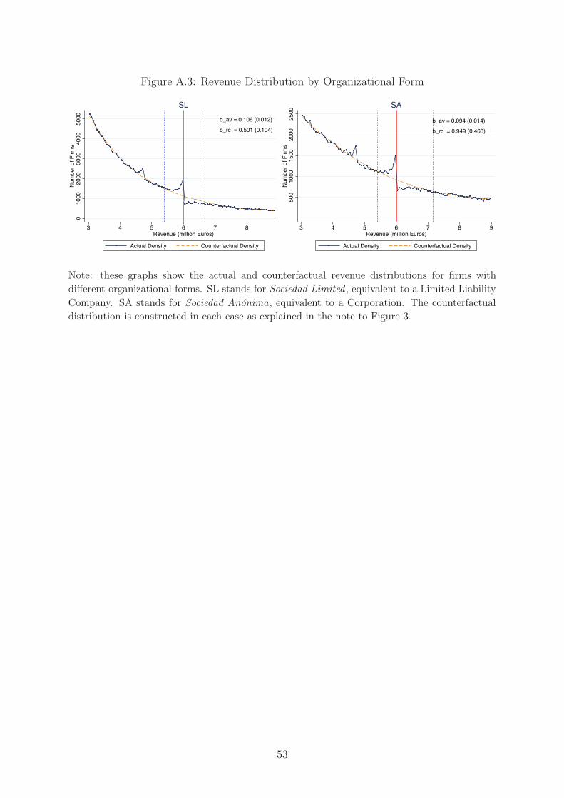
Figure A.3: Revenue Distribution by Organizational Form

b_av = 0.106 (0.012)

b_rc = 0.501 (0.104)

010

0020

0030

0040

0050

00N

umbe

r of F

irms

3 4 5 6 7 8 9Revenue (million Euros)

Actual Density Counterfactual Density

SL

b_av = 0.094 (0.014)

b_rc = 0.949 (0.463)

500

1000

1500

2000

2500

Num

ber o

f Firm

s

3 4 5 6 7 8 9Revenue (million Euros)

Actual Density Counterfactual Density

SA

Note: these graphs show the actual and counterfactual revenue distributions for firms withdifferent organizational forms. SL stands for Sociedad Limited , equivalent to a Limited Liability

Company. SA stands for Sociedad Anónima, equivalent to a Corporation. The counterfactualdistribution is constructed in each case as explained in the note to Figure 3.

53