Heterogeneous (HG) Blankets for Improved Aircraft … Jonathan Bonilla, Chaky Sriranganathan, Junior Villegas, Tony Ponce, Elizabeth Bonnell, Danoosh Kapadia, Diego Benitez, Trevor

Heterogeneous (HG) Blankets for Improved Aircraft

Interior Noise Reduction

Kamal Idrisi

Dissertation submitted to the faculty of the

Virginia Polytechnic Institute and State University

in partial fulfillment of the requirements for the degree of

Doctor of Philosophy

in

Mechanical Engineering

Marty Johnson, Chairman

James Carneal

Rob Clark

Daniel Inman

Alessandro Toso

Ralf Gramlich

November 6, 2008

Blacksburg, VA

Key words: vibration-damping materials and structures, sound isolating elements,

impedance and mobility methods (IMM)

Copyright 2008, Kamal Idrisi

ii

Heterogeneous (HG) Blankets for Improved Aircraft

Interior Noise Reduction

Kamal Idrisi

Marty Johnson, Chairman

Vibrations and Acoustics Laboratories

(ABSTRACT)

This study involves the modeling and optimization of heterogeneous (HG)

blankets for improved reduction of the sound transmission through double-panel

systems at low frequencies. HG blankets consist of poro-elastic media with small,

embedded masses, operating similar to a distributed mass-spring-damper system.

Although most traditional poro-elastic materials have failed to effectively reduce low-

frequency, radiated sound from structures, HG blankets show significant potential.

A design tool predicting the response of a single-bay double panel system

(DPS) with, acoustic cavity, HG blanket and radiated field, later a multi-bay DPS with

frames, stringers, mounts, and four HG blankets, was developed and experimentally

validated using impedance and mobility methods (IMM). A novel impedance matrix

formulation for the HG blanket is derived and coupled to the DPS using an assembled

matrix approach derived from the IMM.

Genetic algorithms coupled with the previously described design tool of the

DPS with the HG blanket treatment can optimize HG blanket design. This study

presents a comparison of the performance obtained using the genetic algorithm

optimization routine and a novel interactive optimization routine based on sequential

addition of masses in the blanket.

This research offers a detailed analysis of the behavior of the mass inclusions,

highlighting controlled stiffness variation of the mass-spring-damper systems inside the

HG blanket. A novel, empirical approach to predict the natural frequency of different

iii

mass shapes embedded in porous media was derived and experimentally verified for

many different types of porous media. In addition, simplifying a model for poro-elastic

materials for low frequencies that Biot and Allard originally proposed and

implementing basic elastomechanical solutions produce a novel analytical approach to

describe the interaction of the mass inclusions with a poro-elastic layer.

A full-scale fuselage experiment performed on a Gulfstream section involves

using the design tool for the positions of the mass inclusions, and the results of the

previously described empirical approach facilitate tuning of the natural frequencies of

the mass inclusions to the desired natural frequencies. The presented results indicate

that proper tuning of the HG blankets can result in broadband noise reduction below

500Hz with less than 10% added mass.

iv

To my parents Jamila and Abderrahman and my grandfather Driss

v

Acknowledgements

First, I would like to express my sincere gratitude to my advisor, Dr. Marty

Johnson, for being an amazing mentor and great friend. Words cannot describe how

thankful I am for having had the opportunity to work with him for the last three years.

I would like to acknowledge my committee member and good friend Dr. Ralf

Gramlich who has been my mentor throughout my undergraduate studies at Technical

University of Darmstadt (TUD). He is the main reason why I wanted to become a Ph.D

in first place.

I would also like to express my gratitude to Dr. James Carneal who was my co-

advisor for the first half of my doctorial studies. Thank you for helping me to grow as a

person and as a researcher.

This project was supported by SMD Corp. under a NASA SBIR grant A2.04-

9836. I am thankful to my committee member and sponsor, Dr. Robert Clark, for

encouraging and supporting me throughout my research. Also, thanks to my co-sponsor

Curtis Michel for the great input throughout the SMD presentations. I would like to

thank my committee members Dr. Daniel Inman as well as Dr. Alessandro Toso for

helping and guiding me every time they had a chance.

I would like to thank the director of the Vibrations and Acoustics Laboratories,

Dr. Chris Fuller coming, who came up with the ‘Heterogeneous Blankets’ idea in first

place. My thesis wouldn’t even exist without him.

Special thanks to Dr. Manfred Hampe and Barbara Seifert at TUD for giving

me the opportunity to study abroad at Virginia Tech as well as for supporting me

throughout the last three years. Also, thanks to Dr. Holger Hanselka for supporting my

future carrerer.

I would like to thank Dr. Paolo Gardonio for the chance to work with him at the

Institute of Sound and Vibration in Southampton over the past summer. I based a lot of

my research on his theories which is why I was honored to work with him in first place.

He is one of the most positive thinking and encouraging professors I have met so far in

my life.

vi

I would especially like to thank Dr. Mike Kidner for all the great input at the

beginning of my doctorial studies. It has been a pleasure to work with him as he is an

expert in the field of poro-elastic media.

Next, I would like to thank the VAL family. It has been a great pleasure

working with them over the past years. I couldn’t think of a better work environment. I

would especially like to thank Gail Coe, my “American mother”, for all the great

support. Thanks to Dan Mennitt for his great input and help as well as for being an

amazing office mate. Special thanks to my colleagues Ben Smith, Tim Wiltgen, Min

Lee for that unbelievable trip to Panama City during Spring Break ’07. I would also

like to thank the various past and current members: Cory Papenfuss, Marcel Remilleux,

Tom Saux, Mark Sumner, Philip Gillett, Elizabeth Hoppe, Yannic Morel, Sean Egger, and

Kyle Schwartz. I wish them all great success in their future academic and professional

lives.

I would also like to thank my former students: Rachel Scott, Parham Sahidi,

Holger Werschnik, Florian Boess, and of course the German dream team Andreas

Wagner and David Bartylla.

Being so far away from home over the last three years would have not been

easy without the support of my friends here in the U.S. My sincere gratitude to my

great friend Judicita Condezo and her parents Oscar and Carmen. I really enjoyed the

time I spend with them at all the family cook-outs, gatherings, etc. This made me feel

like I had a second family here in the U.S. Thank you for that.

I would also like to thank my fellow salseros at SalsaTech for making my stay

at Tech the best time of my life. It was a pleasure to serve as the president of such a

great organization for over two years. Thanks to my performance team dance partner

Erika Kellar for bearing with me for such a long time. Thanks to Brian Murphy for

introducing me to salsa and working with me on my leadership skills. I am also very

grateful for my friendship to Emily Anderson for making me a better person every day

of my life. Thanks especially to my favorite dancer in D.C. Lorena Guerra-Murcia, my

favorite salsa girls in Blacksburg Julia Malapit, Rachel Baldini, Brianna Horricks, and

all my other salsa friends: Diego Cortes, Tamara Chilton, Kelly Gibbs, Jocelyn Casto,

Ilaria Brun del Re, Kate Tressler, Alex Schwartz, Kelsie Ostergarrd, Rachel and

vii

Jessica Wunderlich, Nikolas Sweet, Alejandro Medina, Christin Alleyne, Shelby

Davies-Sekle, Jonathan Bonilla, Chaky Sriranganathan, Junior Villegas, Tony Ponce,

Elizabeth Bonnell, Danoosh Kapadia, Diego Benitez, Trevor kennedy, Emily

Anderson, Kristin Bowers, Kerry Waite, Paul Pallante, and of course one of my

favourite people: Rajesh Thirugnanam. Also, thanks to my non-salsa friends Jamal

Albarghouti, Younes Benchekroun, Wael Hijazi, Saif Rayyan, Melissa Denby, Rangi

Jericevich, William Kaal, Richard Kerr, Brian Stanek, Stephen Daniel, Haitham

Rabadi, Gaith Rabadi, Sven Dorosz, Chanda Leckie and her parents Barbara and Arlen,

Courtney Lynne, and Jon Rice.

I can not forget about my friends back in Germany: Christian Nolda, Lars

Fetzer, Christos Alexandrakis, Joerg Schwab, Harald Zuber, Mathias Nalepa and

Stephan Goessmann. Thanks to my best friend Daniel Theurich for being a loyal and

stand up guy. I couldn’t have done it without him.

At this point I would also like to thank the Virginia Tech writing center for all

the help with my English.

The final words of acknowledgement are reserved for my family. Thanks to my

grandfather Driss for believing in me for all my life. He died the day I first came to

America as the proudest grandfather on earth. It was his dream for me to be the first

Ph.D. in my family and I must say I was very driven by his pride throughout my life.

Thanks to the most important person in my life: my mother Jamila, who is the most

loving and understanding person I know. Thank you for your unconditional love.

Thanks to my father Abderrahman for always having my back no matter what happens.

Knowing that took a lot of pressure off me during my doctorial studies. Special thanks

to Hanan and Iman for being the two greatest sisters ever. I owe everything I achieve in

life to my family’s love, constant support and incredible patience.

viii

Table of Contents

1. INTRODUCTION ........................................................................................1

1.1. Aircraft interior noise ................................................................................................................ 1

1.2. Control of aircraft interior noise............................................................................................... 2

1.3. HG blanket concept.................................................................................................................... 5

1.4. Thesis overview and contributions............................................................................................ 7

2. SINGLE-BAY DOUBLE PANEL SYSTEM...............................................10

2.1. Mathematical model................................................................................................................. 10 2.1.1 Plate mobility matrix ............................................................................................................. 12 2.1.2 Cavity impedance matrix ....................................................................................................... 14 2.1.3 Radiation impedance matrix .................................................................................................. 16 2.1.4 Impedance and mobility matrix for poro-elastic media ......................................................... 17 2.1.5 Matching nodes of the HG blankets, plate and the free field................................................. 21 2.1.6 Input forces ............................................................................................................................ 22 2.1.7 System studied....................................................................................................................... 23 2.1.8 Explicit coupling equations for the system............................................................................ 23 2.1.9 Assembled matrix representation........................................................................................... 25

2.2. Comparison between theory and experiment ........................................................................ 25 2.2.1 Experimental validation for a plate with accelerometer ........................................................ 27

2.2.1.1. Accounting for the mass of the accelerometer ............................................................. 27 2.2.1.2. Experimental results..................................................................................................... 28

2.2.2 Experimental validation for DPS........................................................................................... 29 2.2.3 Experimental validation for DPS with sandwiched HG blanket............................................ 31

2.3. Double HG blankets ................................................................................................................. 35 2.3.1 Single versus double HG blankets ......................................................................................... 36 2.3.2 Weight reduction for double- HG blankets............................................................................ 39

3. MULTI-BAY DOUBLE PANEL SYSTEM .................................................42

3.1. Mathematical model................................................................................................................. 42 3.1.1 Frame and stringers................................................................................................................ 43

3.1.1.1. Mobility matrix for free-free beam ............................................................................... 43 3.1.1.2. Second moment of inertia for frame and stringer......................................................... 44 3.1.1.3. Mobility matrix equations for beam coupled to a plate................................................ 45

3.1.2 Cavity study........................................................................................................................... 47 3.1.2.1. A study on the coupling of two rectangular cavities .................................................... 47 3.1.2.2. A comparison of two cavities inside the MPS .............................................................. 50

3.1.3 Modeling mounts inside MPS................................................................................................ 52 3.1.4 Coupling equations for mounts inside MPS .......................................................................... 53 3.1.5 Fully coupled MPS with HG blankets ................................................................................... 57

3.2. Comparison between theory and experiments....................................................................... 60

ix

4. OPTIMIZATION OF HG BLANKET..........................................................66

4.1. HG blanket design strategies ................................................................................................... 66 4.1.1 Numerical studies on HG blanket .......................................................................................... 67

4.1.1.1. Physical system studied ................................................................................................ 67 4.1.1.2. Modal design................................................................................................................ 68 4.1.1.3. Random and extensive design search ........................................................................... 70

4.1.2 Comparison of results ............................................................................................................ 72 4.1.3 Experimental studies on designed HG blankets..................................................................... 74

4.1.3.1. Experimental investigation on the modal design case.................................................. 74 4.1.3.2. Experimental validation for the design strategies........................................................ 76

4.2. Comparison of optimization routines for the design of HG blankets .................................. 78 4.2.1 System studied....................................................................................................................... 78 4.2.2 Comparison of optimization routines for DPS....................................................................... 79 4.2.3 Iterative method for MPS ...................................................................................................... 82

4.3. Sensitivity of HG blanket design to parameter variation...................................................... 84 4.3.1 Mathematical model .............................................................................................................. 85 4.3.2 Sensitivity study .................................................................................................................... 86

4.3.2.1. Sensitivity study on one DVA ....................................................................................... 87 4.3.2.2. Sensitivity study on two DVAs ...................................................................................... 89

4.3.3 Experimental validation......................................................................................................... 92

5. STUDY ON THE BEHAVIOR OF MASS INCLUSIONS ADDED TO A PORO-ELASTIC LAYER.................................................................................96

5.1. A study on the characteristic behavior of HG blankets ........................................................ 96 5.1.1 FE model and experimental investigation.............................................................................. 96

5.1.1.1. FE model ...................................................................................................................... 97 5.1.1.2. Experimental Investigation .......................................................................................... 97

5.1.2 Parametric studies.................................................................................................................. 99 5.1.2.1. Tuning with varied mass .............................................................................................. 99 5.1.2.2. Tuning with varied stiffness........................................................................................ 100

Mass depth................................................................................................................................ 100 Footprint ................................................................................................................................... 101 Mass interaction distance ......................................................................................................... 104 Effective area............................................................................................................................ 106

5.2. An analytical model for the interaction of mass inclusions with the poro-elastic layer in heterogeneous (HG) blankets............................................................................................................... 112

5.2.1 Mathematical model ............................................................................................................ 113 5.2.1.1. Simplification of the Biot-Allard model for poro-elastic materials............................ 113 5.2.1.2. Modelling of the elastic layer with added mass ......................................................... 115

Numerical evaluation of displacement and stress in 3-direction .............................................. 120 Numerical evaluation of effective stiffness .............................................................................. 121

5.2.2 Results ................................................................................................................................. 125 5.2.2.1. Effective stiffness ........................................................................................................ 125 5.2.2.2. Mass interaction......................................................................................................... 130

6. EXPERIMENTS ON A GULFSTREAM FUSELAGE SECTION .............135

6.1. Preparation of fuselage measurements................................................................................. 135

x

6.2. First fuselage measurements.................................................................................................. 140

6.3. Procedure ................................................................................................................................ 145

6.4. Comparison............................................................................................................................. 147

7. CONCLUSIONS AND FUTURE WORK.................................................154

7.1. Conclusions ............................................................................................................................. 154

7.2. Future work ............................................................................................................................ 159

APPENDIX.....................................................................................................161

A. Experimental measurement techniques - Improved validation of the DPS ........................... 161 A.1. Frame motion....................................................................................................................... 161

Rigidly attached frame .................................................................................................................. 162 Frame on top of foam .................................................................................................................... 164 Hung frame ................................................................................................................................... 165

A.2. Improved preciseness of torque on frame bolts ................................................................... 167 A.3. Improved validation for DPS............................................................................................... 168

B. HG interface ................................................................................................................................ 170

C. Verifying repeatability of poro-elastic media test .................................................................... 172

BIBLIOGRAPHY............................................................................................179

xi

List of Tables Table 2-1: Model parameters of SPS with clamped BC’s used for the exp. validation of the analytical model ....................................................................................................... 28 Table 2-2: Model parameters of the double panel system with two clamped plates. .... 30 Table 2-3: Model parameters of HG blanket and cavity. ............................................. 33 Table 4-1: Average attenuation from 0-500Hz of sound radiated from the trim panel inside a DPS using a porous layer vs. HG-blanket designed with three different strategies ........................................................................................................................ 73 Table 4-2: Average attenuation from 0-500Hz of velocity of the trim panel using three optimization routines ..................................................................................................... 81 Table 4-3: Average attenuation from 0-450Hz of velocity of the trim panel using two optimization routines ..................................................................................................... 83 Table 5-1: Model parameters of the FE model of an HG blanket. ............................... 97 Table 5-2: Parameters and results from masses embedded in “melamine #1a”. ......... 106 Table 5-3: Parameters and results from masses embedded in “melamine #1b”.......... 110 Table 5-4: Linear elastic, isotropic material constants and their expressions in terms of modulus of elasticity E and Poisson´s ratio ν .............................................................. 117 Table 5-5: Material values for evaluation of influence parameters on the effective stiffness ........................................................................................................................ 125 Table 5-6: Comparison between experimental effective stiffness and the predictions of both modelling strategies for the effective stiffness of square, rectangular, and circular mass shapes with different cross-sectional areas......................................................... 127

xii

List of Figures Figure 1-1: Objects incorporated in mathematical model of DPS: Fuselage(1), HG blanket(2), air cavity(3), trim(4) and interior acoustic field(5) ....................................... 3 Figure 1-2: Schematic of plate with acoustic foam mounted on top (a) and measured radiated sound power from the panel with and without passive treatment...................... 4 Figure 1-3: Schematic of plate with: (a) HG blanket mounted on top and (b) schematic of damped mode split effect of the HG blanket on targeted base structure mode. .......... 5 Figure 1-4: Schematic of the development of the HG blanket ........................................ 6 Figure 2-1: Objects incorporated in mathematical model of the double panel system: Fuselage(1), HG blanket(2), air cavity(3), trim(4) and interior acoustic field(5). Interfaces between objects are noted with capital letters A-E. ...................................... 10 Figure 2-2: Schematic of: (a) point force acting off center on a fuselage with 25 output velocities at grid nodes and (b) the 5x5 node points used to compare theory and experiment for the double panel system along with the position of the unit point force excitation........................................................................................................................ 11 Figure 2-3: Notation for velocities and forces on a Plate .............................................. 12 Figure 2-4: 5x5 poro-elastic material model on a plate; Outer nodes (red) of the poro-elastic material model positioned twice the distance away from the inner nodes (green) relative to each other...................................................................................................... 22 Figure 2-5: Experimental setup: schematic (a) and pictures (b) showing the accelerometer position (left) as well as the frame (right), (c) shows the mass position and weight of the HG blanket. ....................................................................................... 26 Figure 2-6: (a) shows the free body diagram of a plate with and without taking the mass m of the accelerometer into account .............................................................................. 27 Figure 2-7: Experimental validation of a clamped plate excited in non center position29 Figure 2-8: Experimental validation of (a) the fuselage and (b) the trim panel of a double panel system measured at 25 points. A unit point force was applied at a non center position on the fuselage panel. ............................................................................ 31 Figure 2-9: Comparison of spatially averaged velocity of a source panel inside a double panel system with and without sandwiched HG blanket. a) predicted response; b) measured response ......................................................................................................... 32 Figure 2-10: Comparison of spatially averaged velocity of a receiving panel inside a double panel system with and without sandwiched HG blanket. a) predicted response; b) measured response..................................................................................................... 34 Figure 2-11: Comparison of experimental and predicted radiated sound power of the receiving side of a DPS with sandwiched HG blanket. Plotted are the spectral density (a) and one-third octave band (b). HG blanket is designed to target the 1-1 mode of the source pane. A unit point force was applied at a non center position on the source panel....................................................................................................................................... 35 Figure 2-12: Experimental configuration of single bay DPS with a) single HG blanket (2’’ thick HG blanket on top of fuselage and 2’’ thick cavity between HG blanket and trim) and b) a double HG blanket (2’’ thick HG blanket on top of fuselage, 1’’ thick HG blanket on top of trim and 1’’ thick cavity in between both HG blankets)............. 36

xiii

Figure 2-13: Measured spatially averaged velocity of the excitation side (fuselage) of a DPS by it self (blue) and with sandwiched single (black) and double (red) HG blanket....................................................................................................................................... 37 Figure 2-14: Experimental vibration response of the receiver side (trim) of a DPS by it self (blue) and with sandwiched single (black) and double (red) HG blanket .............. 38 Figure 2-15: Schematic of the HG blankets used in the double HG blanket experiments. Measured is the fuselage (a) and trim (b) response. ...................................................... 39 Figure 2-16: Experimental vibration response of a DPS. Plotted is the averaged velocity squared of the source panel with no treatment compared to three double HG blankets 40 Figure 2-17: Experimental vibration response of a DPS. Plotted is the spatially averaged velocity of the receiving panel with no treatment compared to three double HG blankets ................................................................................................................... 41 Figure 3-1: 3-D model of multi bay double panel system with sandwiched HG blanket....................................................................................................................................... 42 Figure 3-2: Box- cross section of the beam used for the stringer .................................. 44 Figure 3-3: I-cross section of the beam used for the frame in experimental setup........ 45 Figure 3-4: Free body diagram of a plate with and without beam acting as an individual object.............................................................................................................................. 46 Figure 3-5: (a) MPS with model of two smaller cavities coupled to four HG blankets and additional big cavity block coupled to the trim side; (b) MPS with model of one thick cavity between HG blankets and trim................................................................... 47 Figure 3-6: Pressure squared levels of three air cavities with same base (length x width) dimensions and different thicknesses ............................................................................ 48 Figure 3-7: Free body diagram of two rectangular cavities coupled together ............... 49 Figure 3-8: Pressure squared levels of 0.05m thick cavity vs. two coupled cavities (0.02m + 0.03m thick) ................................................................................................... 50 Figure 3-9: Pressure squared levels of rectangular cavities with various dimensions... 51 Figure 3-10: Two cavities without space in between coupled to a rectangular cavity with same thickness vs. one rectangular cavity with same dimensions......................... 51 Figure 3-11: Figure of a mount modeled in the design tool as a mass-spring/damper-mass system. .................................................................................................................. 52 Figure 3-12: a) Picture of experimental setup to find the mount properties. Mount is set on top of a shaker and a mass connected to an accelerometer was positioned on top of a shaker, b) response of the mount used in the shaker experiment .................................. 53 Figure 3-13: MPS connected with mounts and cavity in between ................................ 54 Figure 3-14: Nodes for the MPS looking through the MPS. The cavity nodes are in the grey area and the mount nodes are presented as red stars. ............................................ 54 Figure 3-15: a) Plot of predicted spatially averaged velocity from 10-105Hz of a coupled multi bay double panel system with mounts and without HG blanket computed at source (fuselage) and receiver (trim) side, b) 3-D model of the computed configuration and c) Animation of the trim (free- free BC, 1), trim mounts (2), fuselage (clamped BC, 3) and fuselage mounts (4) at 62Hz (2nd mode)...................................... 57 Figure 3-16: Schematic of the theoretical MPS model.................................................. 58 Figure 3-17: a) 3-D model of multi bay double panel system with sandwiched HG blanket (1 mass, 17g – top center at each of the four sub sections) and b) operating deflection shape predicted with design tool at 104Hz with fuselage excited at off center

xiv

position and velocity predicted at 130 points throughout the MPS system. Shown is the trim (i), trim mounts (ii), HG blanket with one mass (iii), fuselage mounts (iv) and fuselage panel (v)........................................................................................................... 60 Figure 3-18: 3-D simplified technical drawing of multi bay double panel system ....... 61 Figure 3-19: MPS experimental setup with front (a) and back (b) view. Accelerometers were placed on source and receiving panel as shown in the pictures ............................ 62 Figure 3-20: 3-D model of two cases compared in experimental validation of MPS ... 62 Figure 3-21: Schematic of a) fuselage and b) trim measurement for experimental validation of MPS .......................................................................................................... 63 Figure 3-22: Predicted spatially averaged velocity of the fuselage panel of a MPS with sandwiched porous layer (blue) and with sandwiched HG blanket............................... 63 Figure 3-23: Measured spatially averaged velocity of the fuselage panel of a MPS with sandwiched porous layer (blue) and with sandwiched HG blanket............................... 64 Figure 3-24: Predicted spatially averaged velocity of the trim panel of a MPS with sandwiched porous layer (blue) and with sandwiched HG blanket (red) ...................... 65 Figure 3-25: Measured spatially averaged velocity of the trim panel of a MPS with sandwiched porous layer (blue) and with sandwiched HG blanket............................... 65 Figure 4-1: Schematic of measured source and trim panel. Mass inclusions inside blanket are represented by red dots. Force applied at an off center position, response measured with accelerometer......................................................................................... 68 Figure 4-2: Predicted response of a DPS. Plotted is the spatially averaged velocity of the source and receiving panel from 50-500Hz ............................................................. 69 Figure 4-3: Operating deflection shape of the source panel at its first two resonant frequencies. .................................................................................................................... 69 Figure 4-4: Mass positions of the HG blanket using a) the modal design strategy and b) the best result in terms of attenuation of radiated sound power using the exhaustive design search.................................................................................................................. 70 Figure 4-5: Histogram of the 2500 mass positions vs. attenuation of the sound power radiated from the receiving panel using HG blanket vs. using just porous media ........ 71 Figure 4-6: Schematic of the (top ten) subset of best performers in two layers: top surface and 2.5mmm deep ............................................................................................. 72 Figure 4-7: Predicted response of a DPS. Plotted is the sound radiated from the trim panel with acoustic blanket glued on top and an HG blanket glued on top (modal design vs. best performer in extensive search).......................................................................... 73 Figure 4-8: Experimental vibration response of a clamped DPS. Plotted is the spatially averaged velocity of the fuselage panel with no treatment, an acoustic blanket glued on top and an HG blanket (build with the modal design method) glued on top................. 75 Figure 4-9: Measured response of a clamped DPS. Plotted is the spatially averaged velocity of the trim panel with no treatment, an acoustic blanket glued on top and an HG blanket (build with the modal design method) glued on top................................... 76 Figure 4-10: Predicted response of a DPS. Plotted is the spatially averaged velocity of the trim panel with acoustic blanket glued on top and an HG blanket glued on top (modal design vs. best performer in extensive search).................................................. 77 Figure 4-11: Measured response of a DPS. Plotted is the spatially averaged velocity of the trim panel with acoustic blanket glued on top and an HG blanket glued on top (modal design vs. best performer in extensive search).................................................. 77

xv

Figure 4-12: Schematic of mass positions inside design tool........................................ 78 Figure 4-13: Flow chart of iterative optimization routine ............................................. 79 Figure 4-14: Predicted response of a DPS. Plotted is the spatially averaged velocity of the trim panel with porous media glued on top and an HG blanket glued on top. Compared are three optimization routines..................................................................... 80 Figure 4-15: Predicted response of a MPS trim. The spatially averaged velocity of the trim panel is plotted. The poro-leatic layer case to the two optimization routines is compared........................................................................................................................ 83 Figure 4-16: System to be modelled: mass-spring-damper-system on a plate .............. 84 Figure 4-17: Average velocity in the frequency range from 70Hz-200Hz; DVA targeting the 1-1 mode at 143Hz; crosses symbolize DVA positions on the plate. b) Magnitude of gradient of average velocity describing the change in magnitude (dB) among different DVA positions..................................................................................... 88 Figure 4-18: a) Average velocity in the frequency range from 180Hz-270Hz; DVA targeting the 2-1 mode at 225Hz; crosses symbolize DVA positions on the plate. b) Gradient of average velocity describing the change in magnitude (dB) among different DVA positions. .............................................................................................................. 88 Figure 4-19: a) Average velocity in the frequency range from 270Hz-340Hz; DVA targeting the 1-2 mode at 315Hz; crosses symbolize DVA positions on one quarter of the plate. b) Gradient of average velocity describing the change in magnitude (dB) among different DVA positions..................................................................................... 89 Figure 4-20: a) Average velocity in the frequency range from 320Hz-390Hz; DVA targeting the 3-1 mode at 348Hz; crosses symbolize DVA positions on one quarter of the plate. b) Gradient of average velocity describing the change in magnitude (dB) among different DVA positions..................................................................................... 89 Figure 4-21: Principle of DVA plot concerning different positions.............................. 91 Figure 4-22: Spatially averaged velocity (dB) with first DVA targeting the 1-1 mode and second one targeting the 3-1 mode. Principle of plot is presented in Figure 4-21.. 92 Figure 4-23: Gradient of spatially averaged velocity (dB/DVA position distance) with first DVA targeting the 1-1 mode and second one targeting the 3-1 mode. Principle of plot is presented in Figure 4-21 ..................................................................................... 93 Figure 4-24: Experimental setup and grid for modal hammer excitement (ellipse)...... 94 Figure 4-25: DVA grid for experiments ....................................................................... 94 Figure 4-26: Schematic of HG blanket with mass glued on top of a porous layer........ 95 Figure 4-27: Maximum velocity in the frequency range from 70Hz to 170Hz determined by experiment ............................................................................................. 96 Figure 4-28: Maximum velocity in the frequency range from 70Hz to 170Hz determined by the analytical model. DVA frequency adapted to 139Hz ...................... 96 Figure 5-1: Experimental setup to measure the natural frequencies of the mass inclusions inside the HG blanket. Shown is the data acquisition system (1), the HG blanket (2) and the shaker (3) ...................................................................................... 100 Figure 5-2: Measured transfer function between the input acceleration of the base and output velocity of three different mass inclusions: 11.7g ( ), 18.7g ( ), 27g ( ) ........................................................................................................................ 102

xvi

Figure 5-3: Variation of resonant frequency of an 8 g mass in a melamine foam block as a function of the thickness of foam beneath the mass. Plotted are experimental measurements (+) and a curve fitted through measured data ( )........................ 103 Figure 5-4: (a) Schematic of the HG blanket glued on a base plate moving with the velocity v. (b) An operating deflection shape of a layer of porous media with one mass inclusion (2-D). (c) Force at the base versus the distance x from the middle of the mass inclusion placed at the center of the 150x100x50 mm poro-elastic layer, or the numerical “footprint distance” computation............................................................... 105 Figure 5-5: (a) Schematic of the experimental “footprint distance” measurement, (b) Dimensions of the poro-layer, (c) Natural frequency versus the distance X of the experimental “footprint distance” measurement.......................................................... 106 Figure 5-6: (a) Schematic of numerical estimation of “mass interaction distance” and (b) FE results of natural frequencies of mass inclusions versus mass separation. Plotted is the mode of the first mass ( ), the mode of the second mass ( ), and the natural frequency of a single mass by itself ( )................................................... 108 Figure 5-7: (a) Schematic of the HG blanket experiments used for the “effective area” experiments, and (b) Natural frequencies of different mass shapes measured in shaker experiment. 5.6g ball ( ), 5.8g coin ( ), 5.8g beam ( ), 5.9g square ( ) .......................................................................................................................... 109 Figure 5-8: (a) Schematic of the “effective area” concept and (b) comparison of the “projected” ( ) and the predicted “effective area” ( ) along with the measurements (+) of the ball (a), coin (b), beam (c) and square (d) versus frequency110 Figure 5-9: Experimental validation of “effective area” approach. Shown is the predicted natural frequency for melamine #1a ( ) along with the measurements (+). The coin (1a) and beam (1b) measurement for melamine #1b were used to plot prediction (2, ) for the ball (3a) , square (3b) and an additional shape, a triangle (3c) ............................................................................................................................... 112 Figure 5-10: Comparison of theory ( ) and experiment (+) of “effective area” approach with (1) melamine foam, (2) polyamide, and (3) polyurethane. Measured are the natural frequencies of ball (a), coin (b), triangle (c), beam (d) and square (e). ..... 114 Figure 5-11: Schematic of the “real” HG blanket with a mass glued on top of a poro-elastic layer (a). Approximation with a force F distributed over the area of the mass leading to the pressure distribution p (b) ..................................................................... 119 Figure 5-12: The coordinate system for the “3D Halfspace” of the Boussinesq solution. The force F is applied at a point whose coordinates are described with the vector xf, while the actual position in the material is marked by x. The vector r = x - xf represents the difference of both vectors and has the magnitude R .............................................. 119 Figure 5-13: The Image method leads to the introduction of a limited layer thickness d when 1 2F F= ........................................................................................................... 121 Figure 5-14: Simulation of the displacement in 3-direction at x3 = 0.002m when a force of 1N is distributed over an area of 0.01m x 0.01m .................................................... 127 Figure 5-15: Change of the effective stiffness with the area of the mass shape. A comparison between measurements ( ), predictions of the constant pressure ( ), and constant displacement ( ) model is included for all mass shapes. Part (a) shows the square mass shape, part (b) the rectangular shape with a side length ratio of 1:3, and part (c) the circular shape. ................................................................. 129

xvii

Figure 5-16: Part a) Dependence of the effective stiffness on the side length ratio a:b of an rectangular mass shape. Part b) Dependence of the effective stiffness on the thickness of the poro-elastic layer of the HG blanket. The cross-sectional area of the mass is 0.0001 m2. The evaluation is done with the constant displacement strategy.. 131 Figure 5-17: Prediction of the effective stiffness based on the thickness of the poro-elastic layer and the area of a square-shaped mass...................................................... 132 Figure 5-18: Contour plots of the compressive stress in 3-direction (in Pa) for two applied masses on top of a poro-elastic layer of 0.04 m thickness. Both masses are represented by a pressure p = 104 Pa applied on an area of 0.01 m * 0.01 m and their middle points are 0.08 m away from each other and symbolized in the plots as black quadrangles. Part (a) shows the x2-x3 plane at x1 = 0 (“side view” of the layer) while part (b) shows the stress distribution in the x1-x2-plane at x3 = 0.04 m (“top view” onto the base-plate or fuselage) ........................................................................................... 135 Figure 5-19: Contour plots of the compressive stress in 3-direction (in Pa) for two applied masses on top of a poro-elastic layer of 0.04 m thickness. Both masses are represented by a pressure p = 104 Pa applied on an area of 0.01 m * 0.01 m and their middle points are 0.03 m away from each other and symbolized in the plots as black quadrangles. Part (a) shows the x2-x3 plane at x1 = 0 (“side view” of the layer) while part (b) shows the stress distribution in the x1-x2-plane at x3 = 0.04 m (“top view” onto the base-plate or fuselage) ........................................................................................... 136 Figure 6-1: Section of a Gulfstream fuselage .............................................................. 138 Figure 6-2: Gulfstream fuselage section before (a) and after (b) preparation for final measurements............................................................................................................... 139 Figure 6-3: Poro-elastic cut-outs.................................................................................. 139 Figure 6-4: Drawing of the microphone array, microphones marked with black dots (a) and real microphone array (b) for full scale fuselage measurement............................ 140 Figure 6-5: Side view of fuselage interior. .................................................................. 141 Figure 6-6: Floor sealing (a) and trim connector sheet (b). ......................................... 141 Figure 6-7: Drawing of the experimental setup and the microphone array, microphones marked with black dots (a) accelerometers marked with red dots and picture of fuselage exterior with reference microphone and speaker (b) ................................................... 142 Figure 6-8: Top view of the experimental setup, showing the various positions of the speaker, the reference microphone and the array (I-VI R/L)....................................... 143 Figure 6-9: Picture of the interior of the Gulfstream section with the five skin pockets/ skin pocket groups used for the first measurements .................................................... 144 Figure 6-10: Averaged mobility squared of 1st skin pocket measured at center position excited with modal hammer as shown in left picture .................................................. 144 Figure 6-11: Averaged mobility squared of 2nd skin pocket measured at center position excited with modal hammer as shown in left picture .................................................. 145 Figure 6-12: Averaged mobility squared of 1st group of skin pockets measured at center position excited with modal hammer as shown in left picture.......................... 145 Figure 6-13: Averaged mobility squared of 2nd large group of skin pockets measured at center position excited with modal hammer on two positions as shown in left picture..................................................................................................................................... 146

xviii

Figure 6-14: Averaged mobility squared of 3rd small panel measured at non-center position excited with modal hammer on three positions outside the panel, as shown in left picture .................................................................................................................... 146 Figure 6-15: Histogram of skin pocket cut-on frequencies ......................................... 147 Figure 6-16: Measured spatially averaged squared velocity of a trim panel over ten random points and excited at an off-center position.................................................... 148 Figure 6-17: One of six HG blanket designs (a) obtained with optimization routine and schematic of MPS (b). ................................................................................................. 150 Figure 6-18: Magnitude of the pressure ratio between the 132 microphones (inside the fuselage cabin without trim panel) and the reference microphone from 30-530Hz. Compared is the bare fuselage vs. porous media attached vs. HG blanket attached. .. 151 Figure 6-19: Magnitude of the pressure ratio between the 132 microphones (inside the fuselage cabin without trim panel) and the reference microphone from -1000Hz. Compared is the bare fuselage vs. porous media attached vs. HG blanket attached. .. 152 Figure 6-20: Magnitude of the pressure ratio between the 132 microphones (inside the fuselage cabin without trim panel) and the reference microphone. Compared is the bare fuselage vs. porous media attached vs. HG blanket attached in 1/12 octave band (A-weighted). .................................................................................................................... 153 Figure 6-21: Magnitude of the pressure ratio between the 132 microphones (inside the fuselage cabin with trim panel) and the reference microphone from 40-550Hz. Compared is the bare fuselage vs. porous media attached vs. HG blanket attached. .. 154 Figure 6-22: Magnitude of the pressure ratio between the 132 microphones (inside the fuselage cabin with trim panel) and the reference microphone from 30-1000Hz. Compared is the bare fuselage vs. porous media attached vs. HG blanket attached. .. 155 Figure 6-23: Magnitude of the pressure ratio between the 132 microphones (inside the fuselage cabin with trim panel) and the reference microphone. Compared is the bare fuselage vs. porous media attached vs. HG blanket attached in 1/12 octave band (A-weighted). .................................................................................................................... 155 Figure 6-24: Spatially averaged velocity of skin pocket with cut-on frequency of 125 in 1/12 octave band. Compared is the skin pocket with porous block and with HG blanket. HG blanket has four masses inclusions tuned to 125Hz, 170Hz, 240Hz and 340Hz.. 156 Figure 6-25: Spatially averaged velocity of skin pocket with cut-on frequency of 330Hz in 1/12 octave band. Compared is the skin pocket with porous block and with HG blanket. HG blanket has one mass inclusion tuned to 340Hz...................................... 157 Figure A-1: (a) Comparison of theory vs. experiment of the spatially averaged velocity of a clamped plate with frame mounted to a heavy worktable, (b) picture of the experimental setup, (c) 3-D model of the experimental configuration........................ 163 Figure A-2: (a) Measured plate and frame spatially averaged velocity a clamped plate with frame mounted on a heavy worktable, (b) Picture of experimental setup measuring frame motion on four points while hammering on an off center position ................... 163 Figure A-3: (a) Measured plate and frame spatially averaged velocity a clamped plate with frame placed on top of a 2’’ thick piece of melamine foam, (b) picture of experimental setup measuring frame motion on four points while hammering on an off-center position.............................................................................................................. 164

xix

Figure A-4: (a) Picture of the frame for the single bay experiments hung on a crane, (b) Picture of the modal hammer pointing at the accelerometer position for the hung single bay experiments ........................................................................................................... 165 Figure A-5: (a) Measured plate and frame spatially averaged velocity a clamped plate with hung on a crane, (b) picture of experimental setup measuring frame motion on four points while hammering on an off center position............................................... 166 Figure A-6: (a) Comparison between a clamped plated measurement of the spatially averaged velocity using with (red and blue line) and without (black line) using a torque wrench to mount the plate to the frame, (b) picture of used electronic torque wrench168 Figure A-7: Comparison of the experimental validation of a single bay DPS on the receiver side (trim), excited at a non center position (a) with and (b) without new improvements............................................................................................................... 169 Figure B-1: HG Interface developed for a clearly laid out usage of the developed code for the coupled DPS..................................................................................................... 170 Figure B-2: Material properties in HG interface for DPS ........................................... 171 Figure B-3: Choosing the positions of the masses after choosing the level (height) inside the porous media (left). Plot of the masses (red) inside the porous media (right)..................................................................................................................................... 172 Figure B-4: Some Error Warnings in HG interface..................................................... 172 Figure C-1: Measured transfer function between the input acceleration of the base and output velocity of a single mass inclusion of 5.6g in different porous media blocks (140x140x50mm) from different samples ................................................................... 173 Figure C-2: Resonance frequency for a single mass 5.6g in different porous media blocks (140x140x50mm) from one sample ................................................................. 174

Unless otherwise noted, all images are property of the author.

1. INTRODUCTION There has been substantial research over the last five decades on control of aircraft

cabin noise as private and commercial civil aviation is one of the major categories of

flying. Civil aviation is more then ever an important transportation method for many

people worldwide. The suppression of aircraft interior noise is of major importance as

the environment inside aircrafts affects pilots, crew and passengers. Noise and

vibration inside aircraft cabins cause increasing risks in health and in particular

performance of flight crew and cabin crew as well as a discomfort for the passengers

[1,2]. This thesis presents part of the work that has been done to develop a new passive

noise control device that is used to reduce aircraft interior noise across a broad band

frequency spectrum.

1.1. Aircraft interior noise

Significant process has been made in the last five decades in the understanding,

prediction and control of interior aircraft noise [3]. Aircraft interior noise can be caused

by four major sources: Propeller noise, jet noise, turbulent boundary layer noise and

structure borne noise.

There are many applications in which propeller noise is a serious problem or a

cause for concern. The commercial usage of propeller driven aircraft is limited by high

levels of cabin noise. Propeller noise and can be described by discrete tones at the

fundamental blade passage frequency (BPF) of the engines and its harmonics [4].

These discrete tones are most dominant at low frequencies (below 500 Hz) where

traditional passive treatments have only little effect.

The airborne transmission of jet noise is mainly associated with aircraft that have

wing-mounted engines, and it affects cabin regions aft of the engine exhaust,

particularly when the engines are mounted close to the fuselage. The cabin noise

increases with decreasing the distance of the two engines and the fuselage [3]. An

example of the influence of jet noise is demonstrated in the rear of the passenger cabin

of a Convair 779 airplane which had wing-mounted jet engines is given in [5].

The introduction of turbojet-powered commercial aircraft with flight speeds

much higher then those of propeller driven airplanes have brought the focus on aircraft

2

interior noise control to turbulent boundary layer noise or aerodynamic noise in

general. In 1940 it was recognized that aerodynamic noise is most significant at aircraft

speeds above 200mph [6]. Flight tests have been conducted with driving an airplane

with power off and by measuring twin-engine airplanes in flight level [7,8] and it was

concluded that that aerodynamic noise is a significant contributor to the mid and high

frequency cabin sound pressure levels.

Both, jet noise and turbulent boundary layer noise are broadband and jet noise is

usually present in regions on the rear of the fuselage where boundary layer noise is

shifted to lower frequencies because of the thicker boundary layer. Thus the separation

of this two noise sources to the fluctuating pressures measured on the exterior of an

airplane is a challenge. Cross-spectrum and correlation techniques have been applied to

separate the two contributions to the exterior pressure field on the aft region of the

fuselage of a Boing 737 [9,10].

Engine-induced structure-borne noise caused by out-of-balance forces within the

engines [3] cause vibrations into the fuselage shell which radiate sound into the aircraft

interior. The focus in the last three decades was brought to this noise source

contribution due to the large numbers of jet-powered aircraft with engines mounted

directly on the rear fuselage wall [11]. The structurally excited noise components of the

aircraft take place at the rotating frequencies of the fan and compressor and usually

occur around 75 − 200 Hz [3].

1.2. Control of aircraft interior noise There are several methods to reduce the interior noise levels, including source

reduction, active [12] and passive control of the aircraft transmission paths, and active

control of the sound field [13,14]. Aircraft interior noise has been an important part of

noise control research since the 1930s [15]. A schematic of an aircraft interior

examined in this work is shown in Figure 1-1 consisting of five components: the source

panel or fuselage, HG blanket, air cavity, the receiving panel or trim, and acoustic free

field.

3

Active methods [16,17] have been extensively studied and have been applied in

practice in propeller driven aircraft, but use is limited as passive control systems are

less expensive, less complicated and do not require any control energy.

Figure 1-1: Objects incorporated in mathematical model of DPS: Fuselage(1), HG blanket(2), air cavity(3), trim(4) and interior acoustic field(5)

Passive treatments used in civil aircraft can be broadly grouped into damping

materials and acoustic absorbers. Acoustic barriers are too heavy for aircraft

application. Damping material with different configurations can be mounted on the

fuselage skin [18] as well as to frames, stringers [19] (Figure 1-1(1)) and the trim

panels [20] (Figure 1-1(2)). Parts of the damping material often consist of viscoelastic

material which dissipates energy in addition to adding stiffness and mass. However, it

is also known to have a limited operating temperature range. Although the damping of

viscoelastomers is high, the stiffness of the material changes rapidly with temperature

caused by both external conditions and internal heating due to energy dissipation.

Acoustic absorbers such as fiberglass or polyamide reduce the sound in enclosures by

converting the mechanical motion of the air particles into low-level heat. The control of

low frequency noise in aircraft is a challenge due to the weight and thickness

restrictions imposed on any acoustic treatment. Typically the thickness of a passive

noise control treatment limits the bandwidth over which the treatment will be effective

[21,22]. For example, Baumgartl [23] presented the sound absorbance as a function of

wave frequency for several thicknesses of melamine foam as a function of frequency

and showed that the absorbance was highly dependent upon the thickness of the

treatment and that thick layers are required for the absorption of low frequencies. For

instance, the degree of sound absorption for 50mm thick foam at 500Hz is 0.5 and

drops down rapidly to a absorption value of 0.05 at 100Hz. A measurement conducted

in the Vibrations and Acoustics Laboratories (VAL) by Dr. Johnson and Dr. Carneal

4

shown in Figure 1-2 illustrates once more the weak low frequency performance of

acoustic foam to control the radiated sound of a base plate. Figure 1-2(a) shows the

schematic of the experimental rig used in VAL’s TL facility: Acoustic melamine foam

was mounted on top of an aircraft panel. The sound power radiation of the panel with

and without acoustic foam has been compared. It has been found that passive

treatments positioned inside the fuselage shell of an aircraft, where the fuselage

dimensions limit the thickness of the blankets to a few inches, causes the acoustic

blankets to be ineffective at frequencies below about 500Hz.

a) b)

Figure 1-2: Schematic of plate with acoustic foam mounted on top (a) and measured radiated sound power from the panel with and without passive treatment.

One method to control low frequency transmissions uses damped resonant

devices such as Helmholtz resonators, dynamic vibration absorbers, and tuned vibration

dampers. These have been shown to provide significant reduction at low frequencies

while limiting the added mass to 10% of the untreated structure [24]. However, these

are additional devices that must be used as well as traditional passive treatments.

Another passive control method was the isolation of the interior shell which was

mounted at locations on the floor where the vibration levels were low [25]. This

application has been restricted to relatively small cabins.

From the above analysis, it is evident that an integrated passive solution that can

control noise transmission across the entire bandwidth is needed. One resonant device

developed and tested for broadband control in the last decade is the distributive

vibration absorber which consists of a plate bonded to sound absorbing foam. The

5

b)

resonance of the distributive vibration absorber can be tuned by varying the loading

mass, or the stiffness of the spring. The distributive vibration absorbers were tested on

a cylindrical shell. Experimental results have shown that these devices were very

effective at reducing the vibration response at targeted resonant peaks at lower

frequencies [26]. Once this technology was proven, the natural progression was to

insert the masses inside the porous media instead of mounting the distributive vibration

absorber on top of the porous layer. This way, the stiffness of the poro-elastic material

was used as spring elements of the distributive vibration absorber. This leads to the

development of a new passive control treatment for sound transmission through base

structures, which is called a heterogeneous (HG) blanket.

1.3. HG blanket concept

HG blankets combine the two main passive control mechanisms (damping and

dynamic absorption) into a single control treatment that has the potential to control a

wide frequency range. The HG blanket consists of poro-elastic media such as acoustic

foam with small embedded masses, which act similarly to a distributed mass-spring-

damper-system as seen in Figure 1-3 (a).

Figure 1-3: Schematic of plate with: (a) HG blanket mounted on top and (b) schematic of damped mode split effect of the HG blanket on targeted base structure mode.

a)

6

In present literature, the HG blanket concept evolved through a series of steps,

starting with a single-point absorber (as shown in Figure 1-4(I)), extended to multiple

absorbers acting over a distributed space, (Figure 1-4(II) and ref. [27]), extended

further to multiple masses coupled together (Figure 1-4(III) and refs. [28,29]), and

finally broadened to the full HG concept. In the full HG concept, multiple mass

inclusions are placed inside of a continuous (porous) media to simulate a distributed

mass-spring-damper system (Figure 1-4(IV)) that operates at low frequency where the

blanket is no longer an effective passive absorber. By employing an acoustic treatment

(i.e. the porous media) to provide the stiffness for the mass inclusions, the HG blanket

concept combines both of the main types of passive control mechanisms, damping

(high frequencies) and dynamic absorption (low frequencies), into a single treatment

designed to control a wide frequency range. The acoustic treatment, or porous media, is

a complex structure with coupled fluid and solid properties [30]. However, in the low

frequency regime where the mass inclusions resonate, the polymer matrix or foam

provides the majority of the stiffness that act against the mass inclusions.

Figure 1-4: Schematic of the development of the HG blanket

Recent experimental investigations carried out by Kidner et al.[31,32] as well as

numerical and experimental studies conducted by Sgard, Atalla, and Amedin [33,34]

7

showed that HG blankets have shown significant potential to reduce low frequency

radiated sound from structures, where traditional poro-elastic materials have little effect

[21,22]. This can be accomplished without losing the good performance at high

frequencies due to the porous media. Kidner et al.also came to the conclusion that HG

blankets can be more efficient when the embedded masses are positioned to target

certain modes instead of randomly distributing the masses. In order to target a plate

mode, it is necessary to “tune” the embedded mass to the desired frequency as well as

position it at certain anti-node lines of the mode. “Tuning” the mass insertions can be

achieved by varying the depth of the mass position inside the poro-elastic media, or by

varying the weight and mass shape of the embedded mass [35]. Proper “tuning” of the

masses will result into a mode split of the targeted resonance of the base structure.

Following traditional tuned vibration absorber theory [36], the targeted resonance peak

is then split into two resultant peaks, one above and one below the original peak. If the

damping ratio is correctly designed [37], both resultant resonant frequencies have lower

and more damped amplitudes then the original resonance as shown in Figure 1-3(b).

Note that one can reduce the two “resultant” peaks even more if the damping is

optimized.

1.4. Thesis overview and contributions

As a first step to model the interior of an aircraft with sandwiched HG blanket, a

mathematical model of a single-bay double panel system (DPS) with, acoustic cavity,

HG blanket and radiated field was developed using impedance and mobility methods

(IMM) proposed by Firestone [38,39] and O’Hara [40], further developed by

Gardonio[41]. Panneton and Atalla proposed a model of an acoustic blanket with a FE-

scheme [42]. A novel impedance matrix formulation for the HG blanket is derived and

coupled to the DPS using an assembled matrix approach derived from the IMM [43].

Experimental measurements validated the predicted responses of the source and the

receiver panel due to a point force acting on the DPS [44,45]. As a more rigorous

model of the fuselage interior, the single-bay DPS was then extended to a multi-bay

DPS with frames, stringers, mounts, and four HG blankets [46]. The predicted response

of the animated MPS was compared to measurements and proved viable.

8

This work presents a theoretical and experimental comparison of different design

techniques for allocating the location of embedded masses using the single-bay DPS

[47]. These design techniques include the random placement of the mass inclusions,

placement using a modal design, and an extensive search for the best location for

specific sound transmissions with specific design constraints. Measurements accurately

agree between the results of the modal design and the results of the extensive search

[48]. Genetic algorithms coupled with the previously described design tool of the DPS

with the HG blanket treatment can optimize HG blanket design. This study presents a

comparison of the performance obtained using the genetic algorithm optimization

routine and a novel interactive optimization routine based on sequential addition of

masses in the blanket [49]. After each mass is added, the study requires finding the

optimal location and design for the next mass. When all of the masses are added, the

algorithm then reassesses the design of the first mass and continues until the design has

converged. This technique leads to good attenuation with reduced computational

burden. Variations in mass location and system parameters are investigated. Coupling

between masses modeled as dynamic vibration absorbers (DVA) and the modes of a

clamped rectangular plate probe the sensitivity of the HG blanket design [50].

This study extensively examines the behavior of the mass inclusion inside the

poro-elastic media both numerically and experimentally. The concept of an HG blanket

used to control the sound transmission through double-panel system for aircraft

applications has already been developed in the literature. However, deficiencies in

methodical property control exist and therefore the prime objective of this research is to

provide a simple method to predict and control material properties of the heterogeneous

blankets through alteration of mass and stiffness parameters with the size, varied shape,

and placement of the mass inclusions. Control of these parameters is necessary if

optimized heterogeneous (HG) blankets targeted to specific applications are to be

successfully developed. This research offers a detailed analysis of the behavior of the

mass inclusions, highlighting controlled stiffness variation of the mass-spring-damper

systems inside the HG blanket. Characteristic parameters of the HG blanket like the

“footprint,” “effective area,” and the “mass interaction distance” are defined and

confirmed through mathematical calculations and experimental results [35]. A novel,

9

empirical approach to predict the natural frequency of different mass shapes embedded

in porous media was derived and experimentally verified for many different types of

porous media, including melamine foam, polyurethane, and polyamide [51]. A

maximum error of 8% existed for all the predictions made in this document. In

addition, simplifying a model for poro-elastic materials for low frequencies that Biot

[52] and Allard [53] originally proposed and implementing basic elastomechanical

solutions produce a novel analytical approach to describe the interaction of the mass

inclusions with a poro-elastic layer [54]. The analytical approach formulated with

varied shape of the mass inclusions and the thickness and elastic properties of the poro-

elastic layer predicts the effective stiffness. The experimental validation is included,

and a simplified equation to calculate the effective stiffness of a HG blanket is

proposed. To determine the interaction between two mass inhomogeneities, the stress

field inside the porous material will be evaluated with focus on the stresses at the base

plane (fuselage). These studies are used to gain physical insight into the effect of the

parameters on the performance of the HG blanket, leading to effective optimization and

improved production methodologies

A full-scale fuselage experiment performed on a Gulfstream section involves using

the MPS design tool for the positions of the mass inclusions, and the results of the

“effective area” approach facilitate tuning of the natural frequencies of the mass

inclusions to the desired natural frequencies. The fuselage without any passive

treatment is compared to the cases with added porous media and HG blanket. The

presented results indicate that proper tuning of the HG blankets can result in broadband

noise reduction below 500Hz with less than 10% added mass.

10

2. SINGLE-BAY DOUBLE PANEL SYSTEM A single bay double panel system is modeled and validated in this chapter as a first

step to predict the response of an aircraft interior. An experimental investigation of HG

blanket mounted on both the fuselage and the trim panel is presented.

2.1. Mathematical model

This section presents the mathematical model used to predict the sound radiation

and vibration response of a double panel system with sandwiched HG blanket. The

system investigated consists of 5 components: the fuselage panel or fuselage, HG

blanket, air cavity, the trim panel or trim, and the acoustic free field, which are all

shown in Figure 2-1.

Figure 2-1: Objects incorporated in mathematical model of the double panel system: Fuselage(1), HG blanket(2), air cavity(3), trim(4) and interior acoustic field(5). Interfaces between objects are noted with capital letters A-E.

The fuselage and trim were both modeled as flat plates [55], where the plate

modes from Warburton [56] were used. The foam is modeled using poro-elastic finite

elements based on fundamental fluid, structural, and coupled fluid-structural equations

given by Panneton and Atalla [33,34,57]. A mesh of 8-node brick elements has been

used. The HG blanket itself was developed adding point masses to the poro-elastic

mass matrix. The air cavity is modeled using the modes for a rectangular rigid wall

volume, and the modes are given by Kinsler and Frey [58]. The radiation into the

acoustic free field is modeled as per Elliott and Johnson [60] using an elemental

radiator approach. Note that the diagonal terms lead to a singularity, but the problem

can be avoided as per Bai and Tsao [61] by changing the domain from rectangular to

11

circular in the Rayleigh formula, or as per Berkhoff [62] using the Boundary Element

Method.

To combine the individual models into a system, the forces and velocities at the

interfaces need to be equated. This can be achieved most effectively using the

impedance and mobility method, which couples the components together at discretized

locations on the interfaces. The impedance and mobility method was originally

proposed by Firestone [38,39] and O’Hara [40], further developed by Gardonio and

Brennan [63,64].

For this work, all subsystems were discretized using a 5x5 grid as shown in

Figure 2-2. For a given component, at each frequency, a mobility matrix can be formed

that describes the relationship between all output velocities and all forces in a 25 x 25

matrix. The matrices describing the behavior of each component are calculated by the

aforementioned analytical and finite element models. The detailed derivation of these

matrices is beyond the scope of this paper, and can be found in the references. These

matrices can then be assembled into a larger system matrix, which is described in detail

later.

Figure 2-2: Schematic of: (a) point force acting off center on a fuselage with 25 output velocities at grid nodes and (b) the 5x5 node points used to compare theory and experiment for the double panel system along with the position of the unit point force excitation.

For this derivation, the low frequency assumption is used, i.e. the subsystems of

the double panel system are assumed to be moving with transverse motion only,

therefore moments and axial forces are neglected. In addition, it should be noted that

the panels of a civil aircraft fuselage are curved and coupled through mounts while the

b) a)

12

numerical model in this work assumes flat panels and coupling of the fuselage and trim

panel through the air cavity. This is a common assumption widely used in literature

[66]. The next sections will present the mobility and impedance expressions for the

subsystems as well as the coupling equations used to build the DPS design toll. A

comparison of theory and experiment will prove the mathematical model valid.

2.1.1 Plate mobility matrix

The dynamics of a rectangular plate are considered in terms of a point mobility

matrix. Consider a set of points on the surface of the plate where normal forces are

applied (represented by vector f) and another set of points where normal surface

velocities are measured (represented by vector v) as indicated in Figure 2-3. Therefore,

the velocity and force can be related by the mobility matrix:

v = Mf (2-1)

For a general case the vector v contains the three components of the point

velocity vector ( &u , &v and &w ) and the three angular velocities (θ& x, θ& y and θ& z) but in

this case we take into account only the out-of-plane dynamics. So, the mii term of M

indicates the point mobility at i, while mij indicates the transfer mobility between i

(where v is evaluated) and j (where f is applied).

Figure 2-3: Notation for velocities and forces on a Plate

The mobility matrix can be derived assuming “classical plate theory” for thin

plates. The equation of motion for transverse displacement of a thin plate is

13

4 4 4 2

4 2 2 4 22 ( , , )w w w wD h p x y tx x y y t

ρ⎛ ⎞∂ ∂ ∂ ∂

+ + + = −⎜ ⎟∂ ∂ ∂ ∂ ∂⎝ ⎠ (2-2)

where h is the plate thickness, ρ is the material density, p is the external load applied

and D is the flexural stiffness, defined as:

( )3

212 1EhD

υ=

−, (2-3)

where E and ν are respectively the material Young modulus and Poisson coefficient.

Considering the free vibrations of the plate in vacuum, it is possible to evaluate the

natural frequencies ωmn (integers m and n are the modal numbers) of vibration and the

normal modes given by Warburton [56]. The corresponding mode shapes ψmn with

respect to various boundary conditions are given by Gardonio and Brennan [65]. The

generic term mij of the mobility matrix can be calculated as

( )( ) ( )

( )2 21 1

, ,

1mn i i mn j ji

ijm nj mn

x y x ywm jf j

ψ ψω ω

ω η ω

∞ ∞

= =

= =⎡ ⎤Λ + −⎣ ⎦

∑∑&

(2-4)

where η is the loss factor (η = 2ξ where � is the modal damping) and Λ is the modal

mass which depends on the normalization of the modes and the modes depends on the

boundary conditions. For example for the simply supported case, the modal mass is:

4x yhL Lρ

Λ = (2-5)

where Lx is the plate length and Ly is the plate width. In a real application we are

interested in a limited frequency band so the model indexes are finite such as N and M.

Using the matrix notation (Ψ for the eigenvectors) and defining a diagonal matrix that

contains the denominator and the common term (jω);

=A( )2 21mn

jj

ωω η ω⎡ ⎤Λ + −⎣ ⎦

⎡ ⎤⎢ ⎥⎢ ⎥⎢ ⎥⎢ ⎥⎢ ⎥⎣ ⎦

(2-6)

with N by M modes where n=1 N and m=1 M. The mobility matrix can be written

as: Tv fM = Ψ AΨ (2-7)

14

where Ψv is a N×M×Nv matrix with the eigenvectors evaluated in the measuring points

and Ψf is a N×M×Nf matrix with the eigenvectors evaluated in the forcing points. The

final mobility matrix will be Nv×Nf (number of velocity measurement and force

application points) so is not necessarily square.

2.1.2 Cavity impedance matrix

The pressure field inside the enclosure can be described by the acoustical wave

equation that in its homogeneous form [58,59] is: 2

22 2

1 0ppc t

∂∇ − =

∂ (2-8)

Using the separation of variables, the solution can be written as:

zyxkBkAp ,,cossin)( =+= αααα αααα (2-9)

and

tBtAtp tt ωω cossin)( += (2-10) that leads to the equation:

02

2222 =−++

ckkk zyx

ω (2-11)

hence, the natural resonant frequency for the enclosure:

222

2 zyx kkkcf ++=π

(2-12)

Assuming that the enclosure is rectangular with rigid walls we have:

{ }0+∈= NnL

nk αα

αα

π (2-13)

And the corresponding mode shapes are:

cos cos cosijk ijkx y z

i x j y k zKL L Lπ π π

Φ = (2-14)

The normal modes are orthogonal, so

0 { , , } { , , }{ , , } { , , }ijk mnoV

N

i j k m n odV

V i j k m n o≠⎧

Φ Φ = ⎨ =⎩∫ (2-15)

where VN is the normalization factor. Choosing Kijk equal to

zyxijk LLL

PK 2= (2-16)

where P is the number of nonzero indices, then VN = 1. In order to take into account the

15

forcing terms, the non homogeneous version of (2-8) is considered. And the pressure

field is described by means of the previous mode shapes:

1( , , , ) ( ) ( , , )n n

np x y z t P t x y z

∞

=

= Φ∑ (2-17)

The modal force can be written as:

dStwdS

twdV

tQ

VtF

S ncavityinsideSoursesNo

S nV nn ∫∫∫ ∂∂

−=⎯⎯⎯⎯⎯⎯⎯⎯ →⎯∂∂

−∂∂

= ψψψ 2

2

2

21)( (2-18)

where the first term will be neglected due to the fact that it takes into account the

sources with volume velocity Q and in the examined case there are no sorces inside the

cavity. The velocity on the top surface of the poro-elastic layer (w) is not known as a

function but as a set of discrete values over the FEM grid. Hence, assuming a uniform

acceleration around each node the force can be written as: 2

21

( ) ( , )N

in n i i i

i

wF t x y st=

∂= Φ

∂∑ (2-19)

where si is the area surrounding each node. In the frequency domain, the force can be

written in terms of the velocity field on the top surface of the foam and the prior

equation becomes:

1

( , )( ) ( , )N

i i in n i i i

i

w x yF j x y st

ω ω=

∂= Φ

∂∑ (2-20)

Going into the frequency domain and adding a damping term to eq. (2-8) gives the

following expression: 2

2 2

1

( , )2 ( , )N

i in n n n n n i i i

in

w x ycP P j P j x y sV tρω δ ω ω ω

=

⎛ ⎞ ∂− + + = Φ⎜ ⎟ ∂⎝ ⎠

∑ (2-21)

Hence,

( )2

2 2

1

( , )2 ( , )N

i in n n n i i i

in

w x ycj P j x y sV tρω δ ω ω ω

=

⎛ ⎞ ∂− + + = Φ⎜ ⎟ ∂⎝ ⎠

∑ (2-22)

Solving for the modal pressure amplitude:

( )

2

12 2

( , ) ( , )

2

N

poro i i n i i iin

nn n

c j v x y x y sV

Pj

ρ ω

ω δ ω ω=

⎛ ⎞Φ⎜ ⎟

⎝ ⎠=− + +

∑ (2-23)

using the following vector notation:

1 1 1 2 2 2 1[ ( , ) ( , ) ... ( , )]TN N Nv x y v x y v x y=porov (2-24)

and

16

1 1 2 2 1[ ( , ) ( , ) ... ( , )]Tn n n N Nx y x y x y= Φ Φ ΦnΦ (2-25)

The sum can be written as

1( , ) ( , )

N

poro i i n i i ii

j v x y x y s jω ω=

⎡ ⎤⎢ ⎥Φ = ⎢ ⎥⎢ ⎥⎣ ⎦

∑ Tn poro

\Φ S v

\ (2-26)

and the pressure can be written as: _

( , )nP x ω = poroZv (2-27)

the impedance matrix can finally be described with the following equation:

( )

2

2 22

n

n n

c jV

j

ρ ω

ω δ ω ω

⎡ ⎤⎛ ⎞ ⎢ ⎥⎜ ⎟ ⎢ ⎥⎝ ⎠ ⎢ ⎥⎣ ⎦=

− + +

Tn

\Φ S

\Z

(2-28)

Note that we treated the problem as a “hard” boundary condition:

01=

∂∂np

ρ (2-29)

2.1.3 Radiation impedance matrix

The acoustic power radiated from a structure can be calculated in terms of

normal surface velocity and pressure vectors evaluated on the surface of the vibrating

element as:

Re2S ⎡ ⎤= ⎣ ⎦

HW v p (2-30)

where H refers to Hermitian; on the surface of the source the pressure can be related to

the normal velocity by means of the radiation impedance matrix Z(ω);

=p Zv (2-31) The radiation impedance matrix can be derived using Boundary Element Method or

Rayleigh integral formula in the case of planar sources in a baffle. This leads to the

following expression:

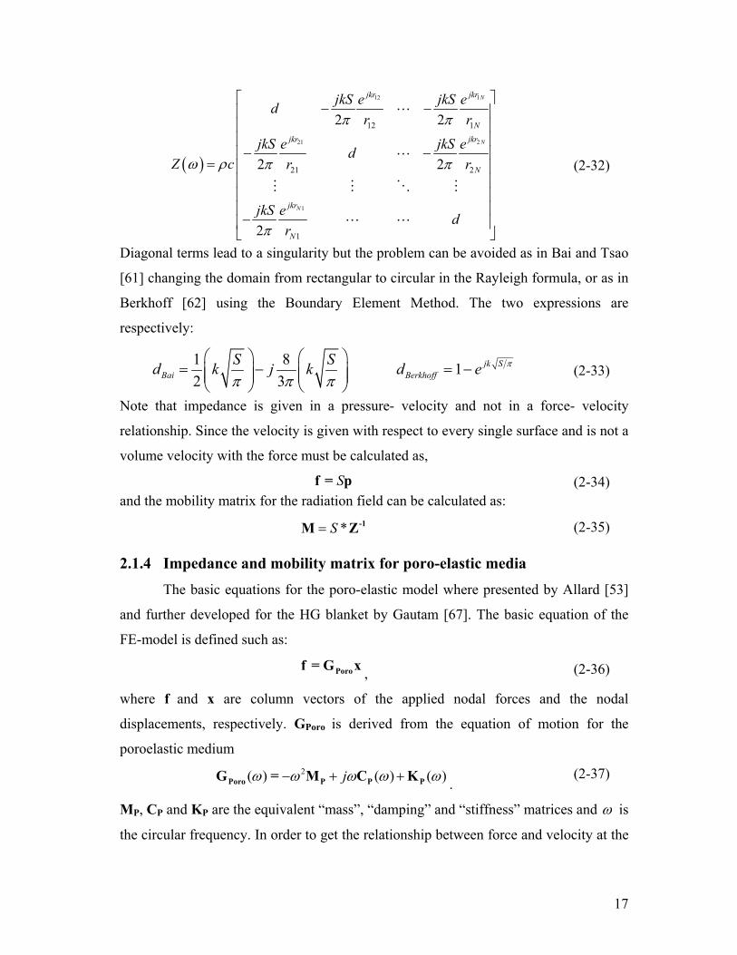
17

( )

112

221

1

12 1

21 2

1

2 2

2 2

2

N

N

N

jkrjkr

N

jkrjkr

N

jkr

N

jkS e jkS edr r

jkS e jkS edZ c r r

jkS e dr

π π

ω ρ π π

π

⎡ ⎤− −⎢ ⎥

⎢ ⎥⎢ ⎥− −⎢ ⎥

= ⎢ ⎥⎢ ⎥⎢ ⎥⎢ ⎥−⎢ ⎥⎣ ⎦

L

L

M M O M

L L

(2-32)

Diagonal terms lead to a singularity but the problem can be avoided as in Bai and Tsao

[61] changing the domain from rectangular to circular in the Rayleigh formula, or as in

Berkhoff [62] using the Boundary Element Method. The two expressions are

respectively:

1 8 12 3

jk SBai Berkhoff

S Sd k j k d e π

π π π⎛ ⎞ ⎛ ⎞

= − = −⎜ ⎟ ⎜ ⎟⎜ ⎟ ⎜ ⎟⎝ ⎠ ⎝ ⎠

(2-33)

Note that impedance is given in a pressure- velocity and not in a force- velocity

relationship. Since the velocity is given with respect to every single surface and is not a

volume velocity with the force must be calculated as,

Sf = p (2-34) and the mobility matrix for the radiation field can be calculated as:

*S= -1M Z (2-35) 2.1.4 Impedance and mobility matrix for poro-elastic media

The basic equations for the poro-elastic model where presented by Allard [53]

and further developed for the HG blanket by Gautam [67]. The basic equation of the

FE-model is defined such as:

Porof = G x , (2-36)

where f

and x are column vectors of the applied nodal forces and the nodal

displacements, respectively. GPoro is derived from the equation of motion for the

poroelastic medium 2( ) ( ) ( )jω ω ω ω ω− + +Poro P P PG = M C K .

(2-37)

MP, CP and KP are the equivalent “mass”, “damping” and “stiffness” matrices and ω is

the circular frequency. In order to get the relationship between force and velocity at the

18

boundary condition nodes (base and top nodes) and the nodes in between, (A.1) can be

written as

⎧ ⎫ ⎧ ⎫⎡ ⎤⎨ ⎬ ⎨ ⎬⎢ ⎥

⎣ ⎦⎩ ⎭ ⎩ ⎭NBC NBC11 12

BC BC21 22

f xG G=

f xG G , (2-38)

with

⎧ ⎫ ⎧ ⎫⎪ ⎪ ⎪ ⎪

⎧ ⎫ ⎧ ⎫⎪ ⎪ ⎪ ⎪⎪ ⎪ ⎪ ⎪⎨ ⎬ ⎨ ⎬ ⎨ ⎬ ⎨ ⎬

⎪ ⎪ ⎪ ⎪⎪ ⎪ ⎪ ⎪⎩ ⎭ ⎩ ⎭⎪ ⎪ ⎪ ⎪⎩ ⎭ ⎩ ⎭

Bs Bs

S SBf Bf

Ts Tsf f

Tf Tf

BC BC

NBC NBCBC BCBC NBC BC NBC

BC BCNBC NBC

BC BC

f x

f xf xf = ,f = , x = , x =

f xf x

f x,

where for the force fBC the first indexes “BC” and “NBC” stand for the boundary

condition and non- boundary condition nodes, respectively and the second indexes

“Bs”, “Bf”, “Ts” and “Tf” stand for the bottom nodes – solid phase/ fluid phase and

the top- nodes solid phase/ fluid phase, respectively. The force and displacement

relationship of the nodes with fixed boundary conditions are obtained by setting the

external force at the non- boundary condition nodes to zero (fNBC=0):

( )-1BC 22 21 11 12 BCf = G - G G G x

. (2-39)

However, since jωBC BCv = x , the impedance at the boundary is given by:

( )1jω

-122 21 11 12Z = G - G G G

, (2-40)

and the mobility matrix is the inverse of the impedance matrix: -1M = Z . (2-41)

Depending on the boundary conditions, the velocity of the fluid phase and solid

phase do not necessarily need to be the same. Therefore it is necessary to split up the

impedance or mobility matrix in a solid-solid phase, solid-fluid phase, fluid-solid phase

and fluid-fluid phase seeing how half of the rows in the impedance or mobility matrix

are due to the fluid phase and the other half due to the solid phase of the poro-elastic

material. The impedance and mobility matrix can then be split up into:

19

⎡ ⎤⎢ ⎥⎣ ⎦

ss sf

fs ff

Z ZZ =

Z Z and ⎡ ⎤⎢ ⎥⎣ ⎦

ss sf

fs ff

M MM =

M M ,

with

⎡ ⎤ ⎡ ⎤ ⎡ ⎤ ⎡ ⎤⎢ ⎥ ⎢ ⎥ ⎢ ⎥ ⎢ ⎥

⎣ ⎦⎣ ⎦ ⎣ ⎦ ⎣ ⎦Bss Bsf Bfs Bff

ss sf fs ffTss Tsf Tfs Tff

Z Z Z ZZ = ,Z = ,Z = ,Z =

Z Z Z Z,

and

⎡ ⎤ ⎡ ⎤ ⎡ ⎤ ⎡ ⎤⎢ ⎥ ⎢ ⎥ ⎢ ⎥ ⎢ ⎥

⎣ ⎦⎣ ⎦ ⎣ ⎦ ⎣ ⎦Bss Bsf Bfs Bff

ss sf fs ffTss Tsf Tfs Tff

M M M MM = ,M = ,M = ,M =

M M M M ,

where the indexes “B” and “T” represent the bottom and top nodes respectively. The

stress and strain relationship for a porous material can be written as

s s s sf fσ = D ε + D ε , (2-42)

hf f f sf sσ = D ε + D ε = p . (2-43)

In which es and ef are strain vectors for the solid and the fluid phases,

respectively and ss and sf are the stress vectors of the solid and fluid phases.

Respectively, where h is the porosity of the poro-elastic material and p is the pore fluid

pressure. Ds, Df, and Dsf are the matrices of the elastic coefficients related to the solid

phase, the fluid phase and the strain coupling between both phases, respectively. The

solid phase stress and strain are the force per unit area and the spatial gradient of the

solid phase displacement. The fluid phase stress is the pressure and the fluid phase

strain is the volumetric strain, or the divergence of the volume displacement. The total

stress on a boundary is the summation of the solid phase and fluid phase stress

s fσ = σ + σ (2-44)

The effective displacement of the boundary depends on if it is a fluid phase or

solid boundary. Consider a very thin layer of fluid phase just in front of the porous

material. The effective velocity at the boundary is (1−h)vs + hvf. In this case the

relationship between the force acting on the porous material and the velocity of the

solid phase at the boundary is given with the mobility matrix Mf such that

(1 )= − +h hf f s fM f v v . (2-45)

20

Consider an infinitesimally thin structural boundary, such that the fluid phase

and solid phase velocities are the same. In this case the relationship between the force

acting on the fluid phase and the total velocity at the boundary is given by the mobility

matrix Ms such that

( )s s s fv = M f + f . (2-46)

The relationship between the solid phase and fluid phase velocities and forces in the

finite element model are

s sf f ss sv = M f + M f , (2-47)

f ff f fs sv = M f + M f , (2-48)

s sf f ss sf = Z v + Z v , (2-49)

f ff f fs sf = Z v + Z v . (2-50)

The total force f applied on the porous material is split into a force applied on the solid

phase fs and on the fluid phase ff, therefore it is assumed that

(1 ) and h h= − =s ff f f f . (2-51)

Hence,

1 hh−⎛ ⎞= +⎜ ⎟

⎝ ⎠s sf ss fv M M f

, (2-52)

1 hh−⎛ ⎞= +⎜ ⎟

⎝ ⎠f ff fs fv M M f

. (2-53)

Using the above equations, the mobility and impedance matrices of a porous material in

contact with an air cavity can be expressed as:

( )2(1 )1 hh h

h−

= + − +f ff fs sf ssM M (M + M ) M, (2-54)

( )12(1 )1 hh h

h

−⎛ ⎞−

= + − +⎜ ⎟⎝ ⎠

f ff fs sf ssZ M (M + M ) M. (2-55)

When calculating the impedance and mobility matrices with solid boundary, the solid

phase velocity vs and the fluid phase velocity vf are equal:

21

s fv = v = v . (2-56)

Hence,

( )s sf ss sf = Z + Z v , (2-57)

( )f ff fs sf = Z + Z v . (2-58)

The mobility and impedance matrices of a porous material in contact with an elastic

structure can be expressed such as:

s sf ss ff fsZ = Z + Z + Z + Z , (2-59)

( )-1s sf ss ff fsM = Z + Z + Z + Z .

(2-60)

The given impedance and mobility matrices in (2-54), (2-55), (2-59) and (2-60)

can be used to describe the HG blanket used in the impedance and mobility method

depending on the boundary conditions.

2.1.5 Matching nodes of the HG blankets, plate and the free field After deriving the individual IMM equations, an interface system must be

developed to interface the plate, heterogeneous blankets, and the acoustic free field.

The problem and solution are now described. The finite element model of the poro-

elastic material has four nodes on each side of an element. However, the radiation

impedance matrix is evaluated at the center of each node. To match the two objects one

could evaluate the velocity at the center of the surface of the finite element model;

however, one could also define a non uniform grid and cut out the outer nodes.

Figure 2-4 shows a simple example of a 5x5 poro-elastic material model (green

and red nodes) on a plate (black nodes). In order to match the radiation mobility matrix,

the outer nodes (red) of the poro-elastic material model have been positioned half the

distance away from the inner nodes (green) relative to each other. Once the impedance

matrix is calculated for the 5x5 matrix, the red nodes will be deleted (by introducing a

new indexing system) and the mobility matrix will be computed with a 3x3 grid size.

Thus if one wants a 5x5 mobility or impedance matrix for the poro-elastic media, the

FE model initially has to create a 7x7 grid.

22

Figure 2-4: 5x5 poro-elastic material model on a plate; Outer nodes (red) of the poro-elastic material model positioned twice the distance away from the inner nodes (green) relative to each other

2.1.6 Input forces

Two main input forces are considered in this thesis, a point force excitation and

plane wave pressure.

The point force excitation is applied on one of the grid points of the left side of

the plate or the bottom surface of the poro-elastic media. Considering the generic

equation that relates the velocity with the force:

),,(),,(),,( ωωω yxfyxMyxv = (2-61)

It is necessary to provide a force in the frequency domain (ω dependency) for

each point to be excited (space dependency). It has been chosen to apply a force with a

unit constant spectrum in the frequency band of interest. In this way it is possible to

find directly the transfer function of the system in terms of velocity over force.

The plane wave pressure that impinges on the left side of the plate or the bottom

surface of the poro-elastic material is considered the blocked pressure (twice the

amplitude of the incident pressure). Considering θ the angle from the vector normal to

the surface and ϕ the angle from the positive x direction on the plate. The incident

plane wave equation [68,69,70] is:

( )( , , ) x yj t k x k yi ip x y t Pe ω − −= (2-62)

23

Where the wavenumber in x-direction is given by sin( ) cos( )xk k θ ϕ= − and the

wavenumber in y-direction is given by sin( ) cos( )yk k θ ϕ= − where c

k ω= is the

wavenumber (c = speed of sound).

2.1.7 System studied

The DPS studied consists of a source and a receiving panel. The source panel,

referred to as the “fuselage,” can be excited with by force or forces. For the work

presented here a unit force acting at x/Lx=0.3 and y/Ly=0.7 on the fuselage panel is

used. The receiving panel is referred to as the “trim” panel.

Figure 2-1 shows the system studied in the mathematical model. The modeled

objects are labeled 1 through 5, which are the fuselage, HG blanket, cavity, trim and

radiation field, respectively. The interfaces of this subsystem are labeled A-E which are

the input force/fuselage, fuselage/HG blanket, HG blanket/cavity, cavity/trim and

trim/radiation field interfaces, respectively.

2.1.8 Explicit coupling equations for the system To couple the objects, a linear system of equations was derived using the

continuity of velocity and equilibrium of forces at all interfaces A E. Mobility and

impedance representations for each object 1 5 were derived. The impedance and

mobility matrices have three indexes. The first index stands for the object number. The

second index points out the interface at which the forces on the objects act. The third

index shows at which interface the velocities are computed. For example, at a given

frequency, the complex mobility matrix M1AB would describe the velocities at interface

B due to forces acting on interface A acting through the first object (1). Hence, M1AB is

a transfer mobility matrix with the input force described by the complex vector fA and

output velocities described by a complex vector vB. Figure 2-2 shows a schematic of

the fuselage with the input point force off center and the 25 output velocities that

describe one column of the mobility matrix M1AB. The impedance matrices Z are

indexed analog to the mobility matrices. The coupling equations for interface B are:

B 1AB A 1BB Bv = M f - M f (2-63)

24

B 2BB B 2BC Cf = Z v + Z v (2-64)

M1BB and fB are the mobility of the fuselage [55] (modeled using analytical

plate equations) and the force acting at the interface B, respectively. Z2BB and Z2BC (see

Appendix A) are derived from the finite element model for the HG blanket. The

equations for interface C are:

C 2CB B 2CC Cf = -Z v - Z v (2-65)

C 3CC C 3CD Df = Z v - Z v (2-66)

Z2CB and Z2CC are also calculated from the finite element model. Z3CC and Z3CD

[58] (calculated using the modes for a rectangular rigid wall volume) are the input and

transfer impedance of the cavity, respectively. The equations for interface D are as

follows:

D 3DC C 3DD Df = Z v - Z v (2-67)

D 4DD D 4ED Ev = M f - M f (2-68)

with Z3DC and Z3DD [58] being the cavity transfer and output impedance respectively.

The coupling equations for the last interface, E, are

E 4DE D 4EE Ev = M f - M f (2-69)

E 5EE Ef = Z v (2-70)

where the mobility matrices of the trim are M4DD, M4DE, M4ED, and M4EE (calculated

similar to the fuselage mobility matrices). The velocity at the trim surface is then

multiplied by the radiation impedance matrix Z5EE (Eq. (8)) as per Elliott et al., Bai et

al. and Berkhoff [60-62] (derived using Boundary Element Method or Rayleigh integral

formula in the case of planar sources in a baffle) to account for radiation loading fE. It

should be noted that in practice, accelerometers were used to measure the fuselage and

trim response. In order to match theory with experiment, these accelerometers were

modeled as lumped masses placed on the plates at the nodes at which the

accelerometers were positioned. The derivation of the explicit coupling matrices makes

it possible to solve for the velocities and forces at the interfaces of interests.

25

2.1.9 Assembled matrix representation There are several potential methods to solve the above set of coupled equations,

from direct algebraic manipulation to a matrix method. Solving for each variable

individually by manipulating (2-63)-(2-70) is a tedious process and prone to

mathematical errors, so it was decided to write the linear set of coupled equations as an

assembled matrix:

⎡ ⎤ ⎡ ⎤⎢ ⎥ ⎢ ⎥⎢ ⎥ ⎢ ⎥⎢ ⎥ ⎢ ⎥⎢ ⎥ ⎢ ⎥⎢ ⎥ ⎢⎢ ⎥ ⎢⎢ ⎥ ⎢⎢ ⎥ ⎢⎢ ⎥ ⎢⎢ ⎥ ⎢

⎢⎢ ⎥ ⎣ ⎦⎣ ⎦

1BB B

2BB 2BC B

2CB 2CC C

3CC 3CD C

3DC 3DD D

4DD 4ED D

4DE 4EE E

5EE E

M I 0 0 0 0 0 0 fI -Z 0 -Z 0 0 0 0 v0 Z I Z 0 0 0 0 f0 0 I -Z Z 0 0 0 v0 0 0 -Z Z I 0 0 v0 0 0 0 I -M M 0 f0 0 0 0 0 -M M I f0 0 0 0 0 0 I -Z v

A1444444444442444444444443{

⎡ ⎤⎢ ⎥⎢ ⎥⎢ ⎥⎢ ⎥

⎥ ⎢ ⎥⎥ ⎢ ⎥⎥ ⎢ ⎥⎥ ⎢ ⎥⎥ ⎢ ⎥⎥ ⎢ ⎥

⎢ ⎥⎥ ⎣ ⎦

1AB AM f000

=0000

x b14243

(2-71)

which can then be solved by inverting the matrix A as well as iteratively. Matrix A is a

sparse and almost block diagonal matrix and therefore efficiently invertible [71].

Taking a closer look at A, one can recognize that it consists of small sub matrices such

as

⎡ ⎤⎢ ⎥⎣ ⎦

3CC 3CD

3DC 3DD

-Z Z-Z Z

(2-72)

which represent the cavity in the observed case. This shows that it is very easy to add

more levels of complexity to an existing system using the matrix formulation, without

needing to use algebraic manipulation.

2.2. Comparison between theory and experiment

This section presents the experimental validation of a DPS with and without the

HG blanket. Figure 2-5 (a) shows the schematic of the experimental setup with the two

clamps (1,6) supporting the clamped boundary conditions of the fuselage (2) and the

trim (5). The HG blanket (3) is attached to the “interior” of the fuselage. A heavy

aluminum block was used as the frame (4). Pictures of the experimental setup in Figure

2-5 (b) show the accelerometer position and grid (left) and the frame (right). A roving

modal hammer excited the fuselage at all of the grid points, and transfer functions from

26

the hammer to accelerometer were measured. Using reciprocity, these can be converted

to a roving accelerometer and a constant position point force excitation, which matches

the model. See Appendix A for more details on experimental techniques.

Figure 2-5: Experimental setup: schematic (a) and pictures (b) showing the accelerometer position (left) as well as the frame (right), (c) shows the mass position and weight of the HG blanket.

Throughout this thesis, the spatially averaged squared velocity of the fuselage

Vf and trim Vt are used to present the predicted response of the double panel system. At

each frequency of interest, Vf and Vt are calculated from 25 by 1 complex vectors of

fuselage and trim velocities vf and vt:

Hf f f

1V = v vN

Ht t t

1V = v vN

(2-73)

These measures are directly proportional to the kinetic energy of the plates as

per Gardonio and Elliott [17]. Furthermore the total sound power radiated from the

double panel system with sandwiched HG blanket can be expressed as follows,

1tP

N= H

t 5EE tv Z v, (2-74)

where Z5EE is the radiation matrix used in (2-70) as per Elliott et al., Bai et al. and

Berkhoff [60-62]. These calculations can then be performed over the frequencies range

of interest (0-500Hz).

27

2.2.1 Experimental validation for a plate with accelerometer In order to validate a complex system such as the DPS with sandwiched HG

blankets, both panels used for the DPS were validated individually. The data of the two

single panels was then used in the analytical model of the DPS. This section presents

the experimental validation of a single plate (used later on as the fuselage panel) with

clamped boundary conditions and a 4g accelerometer placed at an off center position

x/Lx=0.1and y/Ly=0.7 as shown in Figure 2-2(b).

2.2.1.1. Accounting for the mass of the accelerometer

The accelerometer was modeled as a lumped mass and coupled to the plate in

order to build a more accurate mobility matrix for the plate. Figure 2-6 shows the free

body diagram of a plate with and without taking the mass of the accelerometer m into

account.

Figure 2-6: (a) shows the free body diagram of a plate with and without taking the mass m of the accelerometer into account

The equations for the plate modeled with a lumped mass on top of it with an input force

fA and output velocity vA, where the force due to the mass m is fM and the velocity of

the mass at the mass location is vM, solved for vA, is given by:

[ ]→

M 0 M MA A MM M-1

M 0 MM MA A

v = M f = M f - M f

f = M + M M f (2-75)

[ ]⎡ ⎤⎣ ⎦

-1A AA A AM M AA AM 0 MM MA Av = M f - M f = M - M M + M M f (2-76)

M0 is the mobility of the mass m, MAA, MAM , MMA , and MMM are input and transfer

plate mobility matrices with respect to the plate locations (index “A”) and mass

28

locations (index “M”). The output velocity vA in (2-76) which describes the velocity at

all locations on the plate, is expressed as an augmented mobility matrix Mequivalent times

the input force where

[ ]-1equivalent AA AM 0 M M MAM = M - M M + M M (2-77)

2.2.1.2. Experimental results

Table 2-1 presents a list all the important data regarding the experimental test. To

match the experimental fuselage panel in the analytical model, the aspect ratio has been

changed on both plates within 2-3% of the measured values, and the damping ratio for

all modes has been set to 0.006, which is typical for a clamped aluminum plate.

Table 2-1: Model parameters of SPS with clamped BC’s used for the exp. validation of the analytical model

Parameter

Value

Units

Material properties of single plate

Length 0.307 m

Width 0.206 m

Thickness 0.0008 m

Density 2700 kg/m3

Modulus of elasticity 7*1010 N/m2

Poisson’s ratio 0.3 -

Figure 2-7 presents the experimental validation of a clamped plate with the

experimental data presented in Table 2-1. The analytical model matches the experiment

satisfactory in the presented frequency range from 50-1000Hz.

29

Figure 2-7: Experimental validation of a clamped plate excited in non center position

Mequivalent equivalent was used when modeling both the fuselage and the trim

and the result was a better match between the experiment and theory, not only at

higher, but also at low frequencies (below 400Hz), where the additional lumped mass

of the accelerometer would result in an asymmetry of the plate and would let the

uneven modes become more dominant when computing the DPS [72]. Both, the

receiver and the source plate of the DPS were validated individually. The matching

results were similar, hence only the experimental validation of the source plate is

presented.

2.2.2 Experimental validation for DPS This section presents the results of the experimental validation of the coupled

DPS without the HG blanket present. Table 2-2 lists all important properties of the DPS

with two clamped plates used for the experimental validation of the analytical model.

As above, the aspect ratio has been changed on both plates within 2-3% of the

measured values, and the damping ratio for all modes has been set to 0.006.

Figure 2-8 (a) shows the experimental validation of the double panel system on

the fuselage side, excited at x/Lx=0.1 and y/Ly=0.7 as shown in Figure 2-2. Theory and

experiment match very well and the dynamics of the fuselage are all captured with a

high level of detail. Most of the discrepancies can be explained by slight differences in

damping level between experiment and theory. For simplicity, the analytical model

30

uses a constant damping term for all of the modes and the damping was not changed

from mode to mode. This can be particularly seen at the third mode, around 200Hz,

which is much lower in the measured spectrum than in the model. However, the third

experimental mode is an even-odd mode (2-1) [73] which does not couple very well to

the cavity and thus is not very important for sound transmission.

Table 2-2: Model parameters of the double panel system with two clamped plates.

Parameter

Value

Units

Material properties of the Fuselage

Length 0.307 m

Width 0.206 m

Thickness 0.0008 m

Density 2700 kg/m3

Modulus of elasticity 7*1010 N/m2

Poisson’s ratio 0.3 -

Material properties of the Cavity

Thickness 0.1 m

Density 1.2 kg/m3

Speed of sound 343 m/s

Damping 0.01 -

Material properties of the Trim

Length 0.307 m

Width 0.206 m

Thickness 0.0012 m

Density 2700 kg/m3

Modulus of elasticity 7*1010 N/m2

Poisson’s ratio 0.3 -

31

Figure 2-8 (b) presents the experimental validation of the double panel system

on the receiving side, measured at 25 points with the fuselage panel excited at acting at

x/Lx=0.1 and y/Ly=0.7 as shown in Figure 2-2. The comparison shows a good match

across the frequency range of interest (50 to 500 Hz) and should be sufficiently

accurate to capture all of the important physics concerned with sound transmission

through the double panel system. The discrepancies at low frequencies are a result of

minor frame motions which cause a zero in the measured response at around 40Hz. The

frame in the model is assumed to be rigid but the experimental frame, although heavy,

was not perfectly attached to ground. As expected, exact matching between model and

experiment becomes difficult as the system complexity increases.

Figure 2-8: Experimental validation of (a) the fuselage and (b) the trim panel of a double panel system measured at 25 points. A unit point force was applied at a non center position on the fuselage panel.

2.2.3 Experimental validation for DPS with sandwiched HG blanket

This section presents the experimental validation for a DPS with HG-blanket

embedded. The HG-blanket has one mass inserted inside the poro-elastic media, placed

in the center of the plate, near the surface of the poro-elastic media to target the 1-1

mode. This is shown in Figure 2-5(c).

Details of how the embedded masses are tuned to certain natural frequencies are

presented in [35]. The total weight of the embedded masses of all HG blankets

a) b)

32

presented in this paper is approximately 10% of the fuselage panel weight. Other than

the inclusion of the HG blankets, the experimental setup used for the experimental

validation of the double panel system is identical with the one used in this section. Due

to the addition of the HG blanket the cavity thickness is reduced due to the fact that the

distance between fuselage and trim is kept constant. Table 2-3 presents the HG blanket

properties as well as the modified cavity parameters for the experimental validation of

the double panel system with HG blanket inside. The fuselage and trim parameters are

shown on the previous section in Table 2-2.

Figure 2-9 shows the comparison of predicted (a) and measured (b) spatially

averaged velocity of the DPS source panel with and without sandwiched HG blanket.

The HG blanket is designed to target the 1-1 mode of the fuselage at approximately

130Hz. A unit point force was applied at a non center position, shown in Figure 2-6 at

the source panel to excite all plate modes. Theory and experiment show the same

trends: It can be seen that the mode split around 130Hz caused a significant drop in the

vibration response.

Figure 2-9: Comparison of spatially averaged velocity of a source panel inside a double panel system with and without sandwiched HG blanket. a) predicted response; b) measured response

a) b)

33

Table 2-3: Model parameters of HG blanket and cavity.

Parameter

Value

Units

Material properties of the HG blanket

Length 0.298 m

Width 0.198 m

Thickness 0.05 m

Density 50 kg/m3

Modulus of elasticity 2.2*105 N/m2

Poisson’s ratio 0.3 -

Tortuosity 1.7 -

Flow resistivity 3.2*104 Ns/m4

Porosity 0.95 -

Atmospheric pressure 1.0325*105 N/m2

Structural damping 0.0001 -

Viscous characteristic

length 5*10-5 -

Thermal characteristic

length 1.1*10-4 -

Total weight of embedded

masses 23 g

Material properties of the Cavity

Thickness 0.05 m

Density 1.2 kg/m3

Speed of sound 343 m/s

Damping 0.01 -

34

Figure 2-10 shows the comparison of predicted (a) and measured (b) spatially

averaged velocity of the DPS receiving panel with and without sandwiched HG

blanket. One can see that the mode split of the first fuselage mode around 130Hz in

Figure 2-9 caused by the HG blanket, also resulted in a mode split for the first mode of

the trim panel, since the fuselage and trim panels are highly coupled by the air cavity at

this mode. Hence, a drop in the vibration response of the fuselage caused a drop in

vibration response of the trim. It can be seen in Figure 2-10 that the drop in the

vibration response due to the mode split at around 130Hz is quite significant.

Figure 2-10: Comparison of spatially averaged velocity of a receiving panel inside a double panel system with and without sandwiched HG blanket. a) predicted response; b) measured response

Figure 2-11 shows the experimental validation of the power radiated from the

trim panel of the DPS with sandwiched HG blanket. Plotted are the spectral density on

the left and one-third octave band on the right. The results of the experimental

validation in the frequency of interest show that the dynamics of the fuselage are

captured. The results match up well at lower frequencies by duplicating the physics of

the 1-1 mode split on the fuselage. The damping levels do not match perfectly at the

modes but the overall dB level is well matched. From the DPS without the HG blanket

to the DPS with HG blanket, a significant level of complexity has been added to the

analytical model. The one-third octave band plot verifies once again that the theoretical

model captures the basic physics of the system studied.

a) b)

35

Figure 2-11: Comparison of experimental and predicted radiated sound power of the receiving side of a DPS with sandwiched HG blanket. Plotted are the spectral density (a) and one-third octave band (b). HG blanket is designed to target the 1-1 mode of the source pane. A unit point force was applied at a non center position on the source panel

In summary, the above results show that an effective model has been developed

and verified. The results presented using an HG blanket targeting the first mode of the

fuselage also show the potential of the HG blanket to reduce the interior noise levels of

an aircraft by targeting fuselage modes in the low frequency region, i.e. below 500Hz.

In order to make the design tool more user friendly, a user interface was developed

which is presented in Appendix B.

2.3. Double HG blankets Experimental demonstrations of the HG blanket inside the DPS presented in the

previous section have shown that it is possible to control the vibration of the source

panel fairly easy. It seems that the masses inside the poro-elastic media have to be

positioned at the anti-node lines of the source panel and tuned to the right frequencies

to target certain modes of the source panel. Controlling the vibration response of the

receiver panel, by controlling the vibration response of the source panel, was a much

harder task. Every mode in the source panel couples differently into the receiver panel

modes. Some fuselage modes transfer less energy into the system then others as shown

in the “modal” design case in the previous section. The following experiment addresses

this problem by attaching the HG blanket on both, the trim and the fuselage, in order to

control the trim response directly. This is referred to as the “double HG blanket”.

a) b)

36

2.3.1 Single versus double HG blankets

This section compares a DPS with single and double HG blankets inside. Figure

2-12 shows the experimental configuration of the DPS for the double HG blanket

measurements with a) a single HG blanket (2’’ thick HG blanket on top of fuselage and

2’’ thick cavity between HG blanket and trim) and b) a double HG blanket (2’’ thick

HG blanket on top of fuselage, 1’’ thick HG blanket on top of trim and 1’’ thick cavity

in between both HG blankets). The trim has a HG blanket attached that is half as thick

as the HG blanket attached to the fuselage. The fuselage is 0.8mm thick and the trim is

1.2mm thick. This means that the modes of the trim are higher than the fuselage modes.

Thus, the masses inside the HG blanket attached to the trim panel have to be positioned

at a lower depth than the masses inside the poro-elastic media attached to the fuselage.

The HG blankets used in the following experiments are designed to target the first two

modes of the plates they are attached to. This is in reference to the modal design

strategy which will be discussed in section 4.1.1.2.

Figure 2-12: Experimental configuration of single bay DPS with a) single HG blanket (2’’ thick HG blanket on top of fuselage and 2’’ thick cavity between HG blanket and trim) and b) a double HG blanket (2’’ thick HG blanket on top of fuselage, 1’’ thick HG blanket on top of trim and 1’’ thick cavity in between both HG blankets)

Figure 2-13 presents the measured spatially averaged velocity of the fuselage of

a DPS for three cases. With HG blankets on top of both, the trim and the fuselage panel

(red), with an HG blanket on top of the fuselage (black) and just by itself (blue) in the

frequency range of 0-1000Hz. The focus is on the difference between using a single

and a double HG blanket, as the effectiveness of the HG blanket compared to the bare

case was already shown in the previous section. Before looking at this result, one

a) b)

37

would expect that the vibration response of the source panel should not change

significantly, seeing how the configuration on that side has not been changed. The

fuselage is still controlled by the HG blanket. In fact, the response in both cases at low

frequencies is almost identical. However, from 450Hz to 750Hz the response increases

and this could be caused by a different coupling between the two panels. In both

measurements, the poro-elastic media still damps out the vibration response at

frequencies above 500Hz.

Figure 2-13: Measured spatially averaged velocity of the excitation side (fuselage) of a DPS by it self (blue) and with sandwiched single (black) and double (red) HG blanket

Figure 2-14 presents the spatially averaged velocity of the trim of a DPS in

three cases: HG blankets on top of both, the trim and the fuselage panel (red), with an

HG blanket on top of the fuselage (black) and just by itself (blue) in the frequency

range of 0-1000Hz. Again, the focus in this plot is really the comparison between the

single and the double HG blanket configuration. Before looking at the measurements

one would expect improvements when controlling the vibration response of the trim

panel in the DPS directly with the additionally attached HG blanket. First, the HG

blanket is directly attached to the trim and designed to target the first two modes. Prior

results have shown that by reducing the first mode of the fuselage, the first mode of the

trim is reduced. Therefore, a real improvement would only be expected for controlling

the second mode. Second, the poro-elastic media on top of the trim is expected to damp

38

out the response of the trim at frequencies above 500Hz. The layer of poro-elastic

media on top of the trim is very thin, so that the frequency at which the poro-elastic

media will damp out the vibration response of the trim panel is expected to get shifted

to higher frequencies.

Figure 2-14: Experimental vibration response of the receiver side (trim) of a DPS by it self (blue) and with sandwiched single (black) and double (red) HG blanket

The results in Figure 2-14 show the two expected improvements. However, if

one compares the first mode of the trim with and without the second HG blanket on top

of the trim, a large difference can be seen. It was expected that the first mode on the

trim side would not change, seeing how it was already reduced by a significant amount

when using the single HG blanket to control the fuselage. The black line in Figure 2-14

indicates that after splitting the first mode of the fuselage, two modes were created in

both the source and receiver panel that were at a lower amplitude. By attaching the HG

blanket to the trim, one could target either one of these two modes with tuning the mass

inside the poro-elastic media to the right frequency. In other words, the second HG

blanket on top of the trim was really used to split one of the two modes that came out if

splitting the first mode of the fuselage. The vibration response for the first mode

decreased when using the double HG blanket by targeting the first mode of the fuselage

twice. Furthermore, it was possible to target the 2-1 mode of the trim directly with the

HG blanket attached on the trim. It was not possible to target this certain mode by just

39

controlling the fuselage. Finally, in both cases the response of the trim at higher

frequencies was reduced due to the attached poro-elastic media.

In conclusion, a comparison between a single and a double HG blanket inside a

DPS was presented. By attaching a second HG blanket on the trim side, the trim

response could be decreased by a significant amount. At low frequencies, it was

possible to target modes on the trim which were not easy to reduce by just controlling

the fuselage. Additionally, modes that were reduced on the trim side by attaching the

HG blanket on the fuselage could be further reduced by targeting them directly on the

trim.

2.3.2 Weight reduction for double- HG blankets

A comparison between a single and a double HG blanket inside a DPS was

presented in the last section, which led to the following question: Is it more efficient to

design the double HG blankets such that each trim mode is controlled by the HG

blanket on the fuselage side or on the trim side?

In order to answer this question, three double HG blankets were compared (see

Figure 2-15): the first double HG blanket (1) is designed to target the 1-1 mode and the

2-1 mode of both, the fuselage and the trim. The second HG blanket (2) targets the 1-1

mode of the fuselage and the 1-1 mode and the 2-1 mode of the trim. The third HG

blanket (3) targets the 1-1 mode of the fuselage and the 2-1 mode of the trim.

Figure 2-15: Schematic of the HG blankets used in the double HG blanket experiments. Measured is the fuselage (a) and trim (b) response.

Figure 2-16 shows the spatially averaged velocity of the fuselage (schematic

shown in Figure 2-15(a)) of a DPS with and without three different (sandwiched)

double HG blankets. The two yellow arrows highlight the resonant frequencies of the

fuselage targeted with the HG blankets. The green and black line look similar, as both

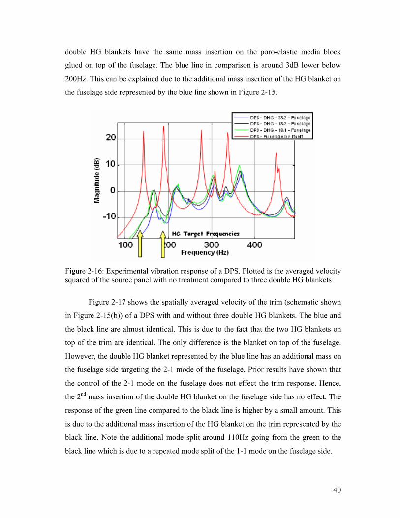
40

double HG blankets have the same mass insertion on the poro-elastic media block

glued on top of the fuselage. The blue line in comparison is around 3dB lower below

200Hz. This can be explained due to the additional mass insertion of the HG blanket on

the fuselage side represented by the blue line shown in Figure 2-15.

Figure 2-16: Experimental vibration response of a DPS. Plotted is the averaged velocity squared of the source panel with no treatment compared to three double HG blankets

Figure 2-17 shows the spatially averaged velocity of the trim (schematic shown

in Figure 2-15(b)) of a DPS with and without three double HG blankets. The blue and

the black line are almost identical. This is due to the fact that the two HG blankets on

top of the trim are identical. The only difference is the blanket on top of the fuselage.

However, the double HG blanket represented by the blue line has an additional mass on

the fuselage side targeting the 2-1 mode of the fuselage. Prior results have shown that

the control of the 2-1 mode on the fuselage does not effect the trim response. Hence,

the 2nd mass insertion of the double HG blanket on the fuselage side has no effect. The

response of the green line compared to the black line is higher by a small amount. This

is due to the additional mass insertion of the HG blanket on the trim represented by the

black line. Note the additional mode split around 110Hz going from the green to the

black line which is due to a repeated mode split of the 1-1 mode on the fuselage side.

41

Figure 2-17: Experimental vibration response of a DPS. Plotted is the spatially averaged velocity of the receiving panel with no treatment compared to three double HG blankets

The main goal of this project is to reduce the sound and vibration of the trim panel

inside the trim panel. All three double HG blankets are designed to target the first two

modes of the DPS. The experimental results show that the double HG blanket can be

designed quite efficiently in terms of reducing the vibration response versus the weight

of the HG blankets: The HG blankets on the two panels need to be designed such that

the trim panel modes which are difficult to control using an HG blanket on the fuselage

side are controlled directly on the trim panel. The modes that are easily controlled by a

HG blanket on the fuselage panel should be targeted directly on the fuselage side. The

results also show that it is very inefficient to target modes on the trim side when they

were already reduced on the fuselage side, like for example the 1-1 mode in the prior

presented case.

Note that there are practical implementation issues associated with the double HG

blankets. Adding HG blankets to aircraft trim panels will result in an increase in

manufacturing costs. Furthermore, the trim panel tends to be more heavily damped than

the fuselage panel, and thus, will respond less to the damping effects of a porous layer.

42

3. MULTI-BAY DOUBLE PANEL SYSTEM The work presented in the last chapter on the design tool included a theoretical

model of a double panel system with a single HG blanket inside. As a step between a

fuselage with multiple skin pockets and the single-bay double panel system (DPS),

more layers of complexity were added to the existing model. This chapter includes a

detailed derivation and analysis of a multi-bay double panel system (MPS) with four

skin pockets and HG blankets of different dimensions including the frames, stringers

and cavity inside the MPS. Finally, this chapter presents a comparison between theory

and experiment of a MPS with sandwiched HG blankets.

3.1. Mathematical model

The mathematical model for the MPS consists of six elements (fuselage,

frame/stringer, HG blankets, mounts, cavity and trim). Figure 3-1 shows a 3-D

computer generated model of the parts that are included. The model is numerated from

(1) – (9). The fuselage (2) is being clamped to a solid structure (3) using four clamps

(1). The stringer (7) and frame (5) are mounted on top of the fuselage without touching

each other (there is a notch inside the frame). Four HG blankets (4) with different

dimensions are glued on top of the fuselage in-between the frame and stringer. Two

angles (6) are attached to the structure (3) in order to hold eight of the twelve mounts

(8) (the other four mounts are held by the frame (5)). A trim (9) built out of aluminum

material was mounted on top of the 12 mounts.

Figure 3-1: 3-D model of multi bay double panel system with sandwiched HG blanket

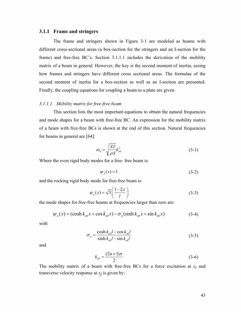
43

3.1.1 Frame and stringers

The frame and stringers shown in Figure 3-1 are modeled as beams with

different cross-sectional areas (a box-section for the stringers and an I-section for the

frame) and free-free BC’s. Section 3.1.1.1 includes the derivation of the mobility

matrix of a beam in general. However, the key is the second moment of inertia, seeing

how frames and stringers have different cross sectional areas. The formulae of the

second moment of inertia for a box-section as well as an I-section are presented.

Finally, the coupling equations for coupling a beam to a plate are given.

3.1.1.1. Mobility matrix for free-free beam

This section lists the most important equations to obtain the natural frequencies

and mode shapes for a beam with free-free BC. An expression for the mobility matrix

of a beam with free-free BCs is shown at the end of this section. Natural frequencies

for beams in general are [64]:

2n nb

EI kS

ωρ

= (3-1)

Where the even rigid body modes for a free- free beam is:

( ) 1n xψ = (3-2)

and the rocking rigid body mode for free-free beam is:

1 2( ) 3nxx

lψ −⎛ ⎞= ⎜ ⎟

⎝ ⎠ (3-3)

the mode shapes for free-free beams at frequencies larger than zero are:

( ) (cosh cos ) (sinh sin )n nb nb n nb nbx k x k x k x k xψ σ= + − + (3-4)

with

cosh cossinh sin

nb nbn

nb nb

k l k lk l k l

σ −=

− (3-5)

and

(2 1)2nb

nk π+= (3-6)

The mobility matrix of a beam with free-free BCs for a force excitation at xi and transverse velocity response at xj is given by:

44

2 21

( ) ( )( (1 ) )ij

n i n j

n n

x xM j

Sl jψ ψ

ωρ ω η ω

∞

=

=+ −∑

(3-7)

3.1.1.2. Second moment of inertia for frame and stringer

The mobility expression in 3.1.1.1 can be used to obtain the mobility matrix

with given mode shapes and natural frequencies. Both the frame and stringer are built

with the same material so the difference really are the cross sectional areas and the

resultant moments of inertia. Figure 3-2 shows a schematic version of the box-cross

section of the beam used as a stringer in the experimental setup.

Figure 3-2: Box- cross section of the beam used for the stringer

The second moment of inertia with bending moment around the y- axis is:

3 31 1 2 2

12Yb h b hI −

=, (3-8)

where the second moment of inertia for the square with the dimensions h1 and b1 are

subtracted from second moment of inertia for the square with the dimensions h2 and b2.

The surface area of the box- section is:

1 1 2 2S b h b h= − (3-9)

Figure 3-3 shows a schematic of the I-cross section of the beam used as a frame in the

experimental setup.

b2

b1

h1 h2

z

y

45

Figure 3-3: I-cross section of the beam used for the frame in experimental setup

The derivation for the second moment of inertia is mathematically more involved as the

I-section used for the MPS experimental rig has two different thicknesses t1 and t2. The

second moment of inertia is: 23 3

1 2 222

12 12 2 2yt h bt thI bt

⎛ ⎞⎛ ⎞= + + +⎜ ⎟⎜ ⎟⎜ ⎟⎝ ⎠⎝ ⎠ (3-10)

With the surface area:

1 2S t h t b= + (3-11)

3.1.1.3. Mobility matrix equations for beam coupled to a plate

In the last chapter the equations for coupling a lumped mass on top of a plate

were given. An equivalent mobility matrix was derived that allowed the mass on top of

the plate and the plate itself to be treated as one single object with one mobility matrix.

Equations for the lumped mass on the plate were used to model the accelerometer used

for the experimental validation of the DPS and gave significantly better results

especially at low and high frequencies.

The previously discussed equivalent matrix method can also be used to couple

larger distributed structures to multiple nodes on the plate. For example, the beams

discussed above were added to the plate using this approach and were coupled to lines

of nodes on the plates. Figure 3-4 shows the free body diagram of a plate with and

without the coupled beam.

h

b

b

t

y

t1 t2

z

46

Figure 3-4: Free body diagram of a plate with and without beam acting as an individual object

The equations for the plate modeled with a beam on top of it, i.e with an input

force fA and output velocity vA and a force due to the beam fB and velocity of the beam

vB, are presented below. Solving for vA:

[ ]0

10

B B BA A BB B

B BB BA A

v M f M f M f

f M M M f−

= = −

⇒ = + (3-12)

[ ] 10A AA A AM M AA AM MM MA Av M f M f M M M M M f−⎡ ⎤= − = − +⎣ ⎦

(3-13)

M0 is the mobility of the beam m. MAA, MAM , MMA , and MMM are input and transfer

plate mobility matrices with respect to the plate locations (index “A”) and beam

locations (index “M”). The output velocity vA in (3-13), which describes the velocity at

all locations on the plate, is expressed as an augmented mobility matrix Mequivalent times

the input force where

[ ] 10equivalent AA AB BB BAM M M M M M−= − + (3-14)

Mequivalent is used to now describe a fuselage panel with beam on top. In the design tool

an equivalent mobility matrix Mequivalent for the stringer on top of the plate was used to

describe the mobility of the fuselage-stringer system. The derived matrix Mequivalent can

then be used as a “new plate mobility matrix” MAA. Therefore, in the case of having

one stringer and one frame, the matrix Mequivalent has to be computed twice iteratively

to add the two components to the plate.

Af

Av

Af

Bf BvBeam

Av

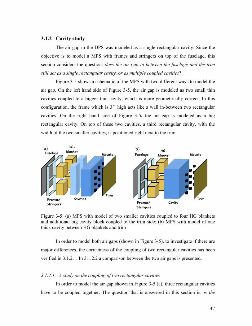
47

3.1.2 Cavity study

The air gap in the DPS was modeled as a single rectangular cavity. Since the

objective is to model a MPS with frames and stringers on top of the fuselage, this

section considers the question: does the air gap in between the fuselage and the trim

still act as a single rectangular cavity, or as multiple coupled cavities?

Figure 3-5 shows a schematic of the MPS with two different ways to model the

air gap. On the left hand side of Figure 3-5, the air gap is modeled as two small thin

cavities coupled to a bigger thin cavity, which is more geometrically correct. In this

configuration, the frame which is 3’’ high acts like a wall in-between two rectangular

cavities. On the right hand side of Figure 3-5, the air gap is modeled as a big

rectangular cavity. On top of these two cavities, a third rectangular cavity, with the

width of the two smaller cavities, is positioned right next to the trim.

Figure 3-5: (a) MPS with model of two smaller cavities coupled to four HG blankets and additional big cavity block coupled to the trim side; (b) MPS with model of one thick cavity between HG blankets and trim

In order to model both air gaps (shown in Figure 3-5), to investigate if there are

major differences, the correctness of the coupling of two rectangular cavities has been

verified in 3.1.2.1. In 3.1.2.2 a comparison between the two air gaps is presented.

3.1.2.1. A study on the coupling of two rectangular cavities

In order to model the air gap shown in Figure 3-5 (a), three rectangular cavities

have to be coupled together. The question that is answered in this section is: is the

Frames/ Stringers

Mounts

Trim Cavity

HG- blanket Fuselage

b)

Trim Frames/ Stringers

Mounts

Cavities

HG- blanket Fuselage

a)

48

continuity of pressure and displacement on the interface nodes of the cavities correctly

included when using the IMM?

In order to prove this, a thick rectangular cavity was compared to two thin

cavities (when coupled together) having the same dimensions as the thick cavity.

Figure 3-6 shows the response of the three cavities (same width and length) with

different thicknesses. Note that the three cavities have modes at the same frequencies

(in the frequency range of interest), since the lower modes are due to the resonant

response of the air along the length and width dimensions of the cavity, and not due to

the thickness. The overall response is lower for the thicker cavities, since the larger

volume leads to less compression of the air, and therefore to less pressure transmitted

across the cavity.

50 100 150 200 250 300 350 400 450

-10

-5

0

5

10

15

20

25

30

35

40

Frequency (Hz)

Pres

sure

squ

ared

leve

ls (d

B)

Cavity TF - 0.05m thickCavity TF - 0.02m thickCavity TF - 0.03m thick

50 100 150 200 250 300 350 400 450

-10

-5

0

5

10

15

20

25

30

35

40

Frequency (Hz)

Pres

sure

squ

ared

leve

ls (d

B)

Cavity TF - 0.05m thickCavity TF - 0.02m thickCavity TF - 0.03m thick

Figure 3-6: Pressure squared levels of three air cavities with same base (length x width) dimensions and different thicknesses

Similar to the principle of an equivalent mobility matrix derived earlier for

lumped masses and beams on top of plates, an equivalent impedance matrix will be

derived to describe the impedance of two cavities coupled together acting as one big

cavity. Figure 3-7 shows the free body diagram of two coupled cavities acting as one

big cavity (a) or acting as two cavities with individual impedance matrices (b).

49

Figure 3-7: Free body diagram of two rectangular cavities coupled together

In order to avoid confusion, the two cavities coupled together will be referred to

as the red cavity and the blue cavity as shown in Figure 3-7. The equations for the

coupled rectangular cavities with an input force fA and output velocity vA, where the

force due to the blue cavity acting on the red cavity is fB and the velocity of the blue

cavity is vB. Solving for fA:

[ ]⇒

B bAB B rBA A rBB B-1

B bAB rBB rBA A

f = Z v = Z v - Z v

v = Z + Z Z v (3-15)

[ ]⎡ ⎤⎣ ⎦

-1A rAA A rAB B rAA rAB bAB rBB rBA Af = Z v - Z v = Z - Z Z + Z Z v (3-16)

The impedance matrices consist of point impedances which are computed for

the nodes at the locations (grid points) at which the two cavities interact. ZbAB is the

transfer impedance of the blue cavity. ZrBA is the impedance of the red cavity from all

locations in the red cavity to the location of the blue cavity, ZrAM is the impedance

from the blue cavity location to all locations on the red cavity, ZrAA is the impedance

matrix that describes all impedances from all locations on the red cavity to all locations

on the red cavity and ZrMM is the red cavity impedance from the blue cavity location to

the blue cavity location. The output velocity vA in (3-17), which describes the velocity

at all locations at the red cavity, is expressed as an augmented impedance matrix

Zequivalent times the input force where:

[ ]-1equivalent AA AB 0 BB BAZ = Z - Z Z + Z Z (3-17)

Af Af

Bf Bv

Av0.03m

0.02m

Av

a) b)

50

Zequivalent can be seen as an equivalent impedance of two coupled cavities. Note that in

the example used in this chapter, the nodes at the locations at which the red and the

blue cavities interact are identical.

Figure 3-8 shows the result of comparing a thick rectangular cavity to two

thinner cavities coupled together. The two cavities were coupled, reversed and coupled

again. The two cavities coupled together have an identical response compared to the

thick cavity, which is independent in the way the two smaller cavities are coupled. This

result proves that two objects described with impedance matrices can be coupled

correctly using the IMM.

Figure 3-8: Pressure squared levels of 0.05m thick cavity vs. two coupled cavities (0.02m + 0.03m thick)

3.1.2.2. A comparison of two cavities inside the MPS

In this section a comparison between a thick cavity and the three thin cavities

shown in Figure 3-5 is presented. Figure 3-9 (a) shows the pressure squared levels of

the two small cavities (black and red, schematic in Figure 3-9 (b)) individually and

acting as a larger cavity next to each other shown in blue. Finally, the pressure squared

levels of a single thin cavity with larger dimensions in width and length is shown in

blue, which has an additional mode at 220Hz due to its larger transverse dimension.

0.03

0.02

0.05

0.03

=

+

=

+

0.02

0 100 200 300 400 500-15

-10

-5

0

5

10

15

20

25

30

35

Frequency (Hz)

Pre

ssur

e sq

uare

d le

vel (

dB)

Cavity TF - 0.05m thickCavity TF - 0.02m + 0.03m thickCavity TF - 0.03m + 0.02m thick

0 100 200 300 400 500-15

-10

-5

0

5

10

15

20

25

30

35

Frequency (Hz)

Pre

ssur

e sq

uare

d le

vel (

dB)

Cavity TF - 0.05m thickCavity TF - 0.02m + 0.03m thickCavity TF - 0.03m + 0.02m thick

51

Figure 3-9: Pressure squared levels of rectangular cavities with various dimensions

Figure 3-10 (a) presents a comparison of the pressure squared levels of the three

cavities coupled together (schematic in Figure 3-10 (b)) to one larger cavity. Both

transfer functions have similar characteristics and modes that lie very close to each

other in terms of frequencies and magnitudes. For the experimental validation of the

MPS, the larger cavity in blue will be used due to shorter computational time.

Figure 3-10: Two cavities without space in between coupled to a rectangular cavity with same thickness vs. one rectangular cavity with same dimensions

b)a)

0 100 200 300 400 500-30

-25

-20

-15

-10

-5

0

5

10

15

Frequency (Hz)

Pres

sure

squ

ared

leve

l (dB

)Cavity TF - 29.5'x14.5'Cavity TF - 13'x14.5'Cavity TF - 15'x14.5'

Vs

+

a) b)

50 100 150 200 250 300 350 400 450

-35

-30

-25

-20

-15

-10

-5

Frequency (Hz)

Pres

sure

squ

ared

leve

l (dB

)

Cavity TF - 1 pieceCavity TF - 2 + 1 pieces

52

3.1.3 Modeling mounts inside MPS As an approximation, the mounts were modeled as a mass-spring/damper-mass

system shown in Figure 3-11. The masses m1 and m2 are connected with a spring and a

damper.

Figure 3-11: Figure of a mount modeled in the design tool as a mass-spring/damper-mass system.

The impedance, Zm1, of the first mass is by definition proportional to the frequency:

1j mω=1mZ (3-18)

The impedance of the spring is inversely proportional to the frequency. And the spring

constant is k. The impedance is:

kjω

=kZ (3-19)

The impedance for the damper is:

c=cZ (3-20)

Analogous to the first mass, the impedance of the second mass is:

2j mω=2mZ (3-21)

Using Firestone’s [74] derivation for impedances in series, the total impedance matrix

for the mounts is:

+1 2

T

m k c m

1Z = 1 1 1+ +Z Z Z Z

(3-22)

In order to obtain the material properties of the mounts used in the later

experimental validation, the mount was analyzed in a shaker experiment. The mount

m1

m2

k c

53

was therefore glued to a shaker. A 12 g steel block and a 1 g accelerometer were then

placed on top of the mount. Figure 3-12 shows a picture of this experiment (a) and the

transfer function of the measurement (b).

Figure 3-12: a) Picture of experimental setup to find the mount properties. Mount is set on top of a shaker and a mass connected to an accelerometer was positioned on top of a shaker, b) response of the mount used in the shaker experiment

The first natural frequency was measured at 25Hz which results in a stiffness

coefficient of k=468.8N/m. The second natural frequency is a rocking mode. Note that

in the model the mount is assumed linear which is not the case if the neoprene-bubble-

mount is deformed excessively.

3.1.4 Coupling equations for mounts inside MPS Modeling the MPS with HG blankets and mounts is different to modeling the

other configurations since the mounts do not touch the HG blanket and are mounted

directly to the fuselage and the trim panel i.e. they bypass the HG blanket and acoustic

cavity. This section first presents the modeling of the MPS without the HG blankets as

an intermediate step. After the impedance of the mounts was derived and the spring

constant was obtained in the prior section, the mounts were incorporated into the MPS.

The most convenient way seems to be the addition of nodes into the system, which

connect the two plates directly with each other without a cavity in between. Figure 3-13

shows the system to be modeled. The fuselage is already modeled as a plate with frame

54

and stringer on top and the only components between the trim and the fuselage are the

cavity and the mounts.

Figure 3-13: MPS connected with mounts and cavity in between

Figure 3-14 shows the top view of the system between the interfaces B and C in

Figure 3-13. The blue nodes marked with a ‘x’ are the 225 cavity nodes. The idea is to

add extra nodes, the mount nodes, noted as red stars in Figure 3-14 that describe the

physics between the two plates connected by this set of mounts.

Figure 3-14: Nodes for the MPS looking through the MPS. The cavity nodes are in the grey area and the mount nodes are presented as red stars.

Fuselage

Trim

Cavity Mounts

A

C

B

1

3

2

0 0.2 0.4 0.6 0.80

0.05

0.1

0.15

0.2

0.25

0.3

0.35

0.4plate/beam/poro grid

x Cavity Nodes

Mount Nodes

55

The key to this derivation of the equations for the coupled MPS with mounts

inside is to understand that the basic equations presented in section 2.1.8 for the DPS

do not change. Instead, the assembled matrix in 2.1.9 gets extended where the number

of added columns and rows is equal to the number of mounts added to the system. The

explicit set of equations, not including the HG blanket, are:

B 1AB A 1BB Bv = M f - M f (3-23)

Cav Cav Cav Cav CavB 2BB B 2BC Cf = Z v - Z v (3-24)

Cav Cav Cav Cav CavC 2CB B 2CC Cf = Z v - Z v (3-25)

c 3CC cv = M f (3-26)

M1AB and M1BB are the mobility matrices of the fuselage [55]. Z2CCcav, Z2CDcav Z2DCcav

and Z2DDcav [58] are the input and transfer impedance matrices of the cavity. The

mobility matrix of the trim M3CC is analogous to the mobility matrix of the fuselage

just with different BCs. In addition to the presented set of equations, an additional set

of equations was derived to describe the interaction between the plates and the mounts

in the MPS:

M M M M MB 2BB B 2BC Cf = Z v - Z v (3-27)

M M M M MC 2CB B 2CC Cf = Z v - Z v (3-28)

The input and transfer impedance matrices of the mounts are Z2CCM, Z2CDM Z2DCM and

Z2DDM. The velocity and force vectors vB, vC, fB and fC include both, the cavity and

mount nodes:

, , ,Cav Cav Cav Cav

M M M M

B C B C

B C B CB C B C

v v f fv v f f

v v f f

⎧ ⎫ ⎧ ⎫ ⎧ ⎫ ⎧ ⎫⎪ ⎪ ⎪ ⎪ ⎪ ⎪ ⎪ ⎪= = = =⎨ ⎬ ⎨ ⎬ ⎨ ⎬ ⎨ ⎬⎪ ⎪ ⎪ ⎪ ⎪ ⎪ ⎪ ⎪⎩ ⎭ ⎩ ⎭ ⎩ ⎭ ⎩ ⎭

(3-29)

The assembled matrix comes out to be the following:

(3-30)

56

{

⎡ ⎤⎢ ⎥

⎡ ⎤ ⎡ ⎤⎢ ⎥ ⎡ ⎤⎢ ⎥ ⎢ ⎥⎢ ⎥ ⎢ ⎥⎢ ⎥ ⎢ ⎥⎣ ⎦ ⎣ ⎦⎢ ⎥ ⎢ ⎥⎢ ⎥ ⎢ ⎥⎡ ⎤ ⎡ ⎤⎢ ⎥ ⎢ ⎥⎢ ⎥ ⎢ ⎥⎢ ⎥ ⎣ ⎦⎢ ⎥ ⎢ ⎥⎣ ⎦ ⎣ ⎦⎢ ⎥⎢ ⎥⎣ ⎦

Cav Cav

M M

Cav Cav

M M

1BB

2BB 2BCB

2BB 2BC B

C2CB 2CC

C2CB 2CCX

3CC

A

M I 0 0-Z 0 Z 0 fI 0

0 -Z 0 Z vf-Z 0 Z 0

0 I v0 -Z 0 Z

0 0 I -M1444444444442444444444443

In order to check the correctness of the code for the MPS with the mounts

included, the operating deflection shape of the system was observed at chosen

frequencies. Figure 3-15 presents a plot of the predicted velocity from 10-105Hz of a

coupled MPS with mounts (without HG blanket) computed at fuselage and trim panel

(a). It also presents the 3-D model of the computed configuration (b) and the operating

deflection shape of the trim (free-free BC, (1)), trim mounts (2), fuselage mounts (3)

and fuselage plate (clamped BC, 4) at 62Hz (2nd mode, (c)). It was found to be more

useful to present the operating deflection shape of the mount nodes independent from

the panel nodes to ensure a realistic movement of the mounts. The fuselage moves in a

2-1 mode, where the plate is divided into four skin pockets due to its frame and

stringer. As expected the trim panel which seems to have small amplitude at the mount

points and deformed at all the non-mount points implying that the main mechanism of

excitation at this resonance is through the acoustic cavity.

57

Figure 3-15: a) Plot of predicted spatially averaged velocity from 10-105Hz of a coupled multi bay double panel system with mounts and without HG blanket computed at source (fuselage) and receiver (trim) side, b) 3-D model of the computed configuration and c) Operating deflection shape of the trim panel (free- free BC, 1), trim mounts (2), fuselage mounts (3) and fuselage panel (clamped BC, 4) at 62Hz (2nd mode)

In conclusion, the assembled matrix for the MPS including mounts was derived

and the predicted response was analyzed to assure the correctness of the design tool.

The next step is the incorporation of the HG blanket into the design tool.

3.1.5 Fully coupled MPS with HG blankets This section presents the coupling equations for the final MPS design tool with

both mounts and HG blanket. The operating deflection shape of the complete MPS

system will be presented at a chosen frequency.

Figure 3-16 presents a schematic of the theoretical model for the MPS design

tool. The interfaces are denoted A, B, C and D. The frame and stringer are modeled as

beams attached to certain nodes of the fuselage. These nodes are denoted with “I”. The

frame and stringer are directly coupled to the cavity; hence the frame and stringer are in

between the interface B and C. The HG blanket is coupled to the fuselage and the

20 40 60 80 100

-60

-50

-40

-30

-20

-10

Frequency (Hz)

Spa

tially

ave

rage

d ve

loci

ty (d

B)

coupled fuselagecoupled trim

b)

c) a)

4

3

2

1

58

cavity. The HG blankets nodes are denoted as “II”. The cavity which is coupled to the

frame and stringer and the HG blanket includes both nodes “I” and “II”. The mounts

are coupled to the fuselage and the trim panel. The nodes for the mounts are denoted

with “III”.

Figure 3-16: Schematic of the theoretical MPS model

The key to the MPS derivation is to understand that the system has to be broken

down into the three node groups. Each of these node groups couples different parts of

the MPS. Once the problem is setup as shown in Figure 3-16, the derivation of the

IMM coupling equations becomes fairly straight forward. The fuselage is coupled to all

three node groups as shown in (3-31):

⎧ ⎫ ⎧ ⎫ ⎧ ⎫⎪ ⎪ ⎪ ⎪ ⎪ ⎪⎨ ⎬ ⎨ ⎬ ⎨ ⎬⎪ ⎪ ⎪ ⎪ ⎪ ⎪⎩ ⎭ ⎩ ⎭ ⎩ ⎭

F F

B,I A,I B,I

B,II AB A,II BB B,II

B,III A,III B,III

v f fv = M f - M fv f f

(3-31)

The sub index “F” represents the fuselage. The fuselage is then coupled to the HG

blankets (“HG”) and the mounts (“M”). The HG blankets are coupled to the cavity in

(3-32) and (3-34), the mounts are directly coupled to the trim panel in (3-33):

B,II 2BB B,II 2BC C,IIf = Z v + Z v (3-32)

M MB,III BB B,III BD D,IIIf = Z v -Z v (3-33)

C,II 2CB B,II 2CC C,IIf = Z v + Z v (3-34)

59

The cavity (“Cav”) couples the frame, stringer and the HG blankets to the trim panel

(3-35) and (3-36) which is attached to the mounts as shown in (3-37):

⎧ ⎫ ⎧ ⎫ ⎧ ⎫⎨ ⎬ ⎨ ⎬ ⎨ ⎬⎩ ⎭ ⎩ ⎭ ⎩ ⎭

Cav Cav

B,I B,I D,ICC CD

C,II C,II D,II

f v v= Z -Z

f v v (3-35)

⎧ ⎫ ⎧ ⎫ ⎧ ⎫⎨ ⎬ ⎨ ⎬ ⎨ ⎬⎩ ⎭ ⎩ ⎭ ⎩ ⎭

Cav Cav

D,I B,I D,IDC DD

D,II C,II D,II

f v v= Z -Z

f v v (3-36)

M MD,III DB B,III DD D,IIIf = Z v -Z v (3-37)

Finally, the mobility matrix representing the free-free trim panel couples the velocities

and forces of all node groups as shown in (3-38):

⎧ ⎫ ⎧ ⎫⎪ ⎪ ⎪ ⎪⎨ ⎬ ⎨ ⎬⎪ ⎪ ⎪ ⎪⎩ ⎭ ⎩ ⎭

T

D,I D,I

D,II DD D,II

D,III D,III

v fv = M fv f

(3-38)

The reason why this is still a fully coupled system is once again because the

fuselage and trim matrices are fully populated. This takes care of describing the

different interactions between the mounts, HG blankets and cavity dynamics to the

fuselage and trim panel. It was decided for brevity not present the assembled matrix

derived from the coupling equations. The matrix consists of 14x14 components which

exceeds the size of a page.

One way to analytically verify the MPS design tool is to look at the operating

deflection shape of the MPS at various frequencies and look if the predicted behavior is

realistic and similar to the deflection shapes presented in the last section. Figure 3-17

presents a 3-D model of multi bay double panel system (a) with sandwiched HG

blankets (1 mass, 23g – top center at each of the four sub sections) and the operating

deflection shape (b) predicted with the design tool at 104Hz, with the fuselage excited

with a point force at an off center position and velocities predicted at 130 points

throughout the MPS system. Shown is the trim (i), trim mounts (ii), HG blanket with

one mass (iii), fuselage mounts (iv) and fuselage panel (v).

60

Figure 3-17: a) 3-D model of multi bay double panel system with sandwiched HG blanket (1 mass, 17g – top center at each of the four sub sections) and b) operating deflection shape predicted with design tool at 104Hz with fuselage excited at off center position and velocity predicted at 130 points throughout the MPS system. Shown is the trim (i), trim mounts (ii), HG blanket with one mass (iii), fuselage mounts (iv) and fuselage panel (v)

The frame and stringer on top of the fuselage divide the plate into four skin

pockets, with each of the quadrants moving as a single plate by itself. At the chosen

frequency two of the four quadrants on each of the two sides divided by the stringer are

moving in phase (v). In (iii) the top surface of the HG blankets is animated. The four

masses at each of the four quadrants, when excited, are moving up and down while two

of each side move in phase and both masses on each side move out of phase. It was

found to be more interesting to plot the mount nodes independent from the panel nodes

(ii, iv). Once again, similar to the results shown in the previous section, the trim (i)

seems to have reduced amplitude at the mount points and deformed at all the non-

mount points.

3.2. Comparison between theory and experiments

This section presents a comparison of predicted and measured spatially

averaged velocity of both the fuselage and the trim response due to a point force

excitation on the fuselage panel.

a) b)

(ii)

(iii)

(iv)

(v)

(i)

61

As shown previously, Figure 3-1 shows a 3-D computer generated model of the MPS

experimental rig without the trim panel. The outer dimensions of the solid structure are

42’’ x 21.5’’ x 4’’ with 1’’ thick walls. The clamps (1) holding the fuselage (2) to the

structure (3) have thin slots inside in order to increase the pressure acting on the

fuselage (2). The stringer (7) has a box-cross section with outer dimensions of 1’’ x 1’’

and the frame (5) has an I-cross section with the dimensions 1.5’’ x 3’’. The frame (5)

and angles (6) are the support for the neoprene mounts (8) with a height of 0.75’’ and a

maximum diameter of 0.256’’. The four areas for the poro-elastic media are: 10’’ x

17.5’’, 8.5’’ x 17.5’’, 10’’ x 21’’ and 8.5’’ x 21’’ which are reasonably close to the

Gulfstream fuselage in the VT facilities presented in chapter 5. A simplified technical

drawing of the MPS without the trim panel including the most important dimensions is

shown in Figure 3-18.

Figure 3-18: 3-D simplified technical drawing of multi bay double panel system

Figure 3-19 presents the picture of the front (a) and the back (b) view of the

complete MPS experimental rig. The MPS fuselage which is clamped to a heavy

aluminum block is 0.8mm thick. The aluminum trim panel is 1.2mm thick and mounted

on top of twelve mounts and sealed with tape on the edges. The accelerometer is placed

Stringer: 1’’x1” Frame: 3’’x1.5”- I Section

42’’

21.5’’

10’’

8.5’’ 21’’

17.5’’

4’’

8.5’’x21’’

8.5’’x17.5’’

10’’x17.5’’

10’’x21’’

Mount 0.256" (Diameter)

1’’

1’’

1’’

1’’ 1.5’’

62

off center, close to the upper left edge on the fuselage panel and close to the upper right

edge on the trim panel. The MPS was excited at 121 points on the fuselage side.

Figure 3-19: MPS experimental setup with front (a) and back (b) view. Accelerometers were placed on source and receiving panel as shown in the pictures

The fuselage has four skin pockets, due to the frame and stringer. The four HG

blankets placed on the skin pockets are chosen to not be completely identical in terms

of the mass inclusion configuration. The two largest skin pockets have a 17g mass on

top of the poro-elastic media. The third and fourth largest skin pockets have an HG

blanket with a 14g and 11.3g mass inclusion on top of the poro-elastic block,

respectively. All mass inclusions are placed on the center of each poro-elastic block to

target the 1-1 mode of each skin pocket. Figure 3-20 shows a 3-D model of the two

cases compared in both theory and experiment: MPS and poro-elastic media with and

without mass inclusions.

Figure 3-20: 3-D model of two cases compared in experimental validation of MPS

accelerometer accelerometer

b)

14g

11.3g

17g

a)

63

Figure 3-21 presents a schematic of the side view of the MPS with measured

fuselage (a) and trim panel (b). Note that in the prediction, a point force was applied at

an off center position; however, the velocities were predicted at 121 points. In the

measurement, a point force was applied at each of the 121 node points using a modal

hammer and the velocities due to each point force are measured and spatially averaged.

This is essentially the same due to reciprocity.

Figure 3-21: Schematic of a) fuselage and b) trim measurement for experimental validation of MPS

The predicted spatially averaged velocity of the fuselage of a MPS with

sandwiched poro-elastic material vs. HG blankets targeting the 1-1 mode of each of the

four sub panels is shown in Figure 3-23. The HG blankets reduce the fuselage vibration

around 100-170Hz and around 250Hz. Note that the HG blankets are not optimized.

Once the HG blankets are tuned to the right natural frequency, they have potential to

reduce the fuselage response by a significant amount.

Figure 3-22: Predicted spatially averaged velocity of the fuselage panel of a MPS with sandwiched porous layer (blue) and with sandwiched HG blanket

100 150 200 250 300 350 400 450 500-50

-45

-40

-35

-30

-25

Frequency (Hz)Spat

ially

ave

rage

d ve

loci

ty (d

B)

PoroHG blanket

64

Figure 3-23 shows the measured spatially averaged velocity of the fuselage

panel of a MPS with sandwiched poro-elastic layer (blue) and with sandwiched HG

blankets (red) from 70-500Hz. Just like in the prediction in Figure 3-22 the

measurement shows a decrease in vibration response around 100-170Hz and around

250Hz. The vibration level of both predictions and measurements are similar, and the

dynamics are captured to a reasonable level of detail considering that the MPS design

tool describes a fairly complicated system with six structural/acoustic components that

are coupled.

Figure 3-23: Measured spatially averaged velocity of the fuselage panel of a MPS with sandwiched porous layer (blue) and with sandwiched HG blanket

The predicted spatially averaged velocity of the trim panel inside the MPS with

sandwiched poro-elastic material vs. HG blankets is presented in Figure 3-24. The HG

blankets reduce the vibration response of the trim panel around 100-170Hz and around

235Hz similar to the fuselage panel. After 360Hz, the trim response does not change.

This does make sense as the HG blankets are tuned to frequencies below 260Hz.

Figure 3-25 shows the measured spatially averaged velocity of the trim panel of

a MPS with sandwiched poro-elastic layer (blue) and with sandwiched HG blankets

(red) from 50-400Hz. The vibration level is similar in both prediction and

measurement. One can see the effect due to the mass inclusions between 100- 200Hz.

However, at higher frequencies, both measured curves are dissimilar, which could be

due to repeatability or flanking issues in the experimental setup. The trim panel is

mounted on top of 12 mounts and sealed with tape. Each measurement involves taking

the trim panel off and then replacing it, in order to add the mass inclusions inside the

100 150 200 250 300 350 400 450 500-50

-45

-40

-35

-30

-25

Frequency (Hz)Spat

ially

ave

rage

d ve

loci

ty (d

B)

PoroHG blanket

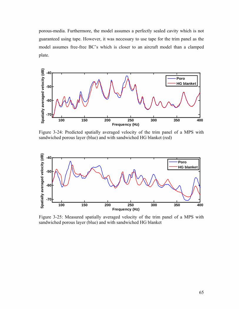
65

porous-media. Furthermore, the model assumes a perfectly sealed cavity which is not

guaranteed using tape. However, it was necessary to use tape for the trim panel as the

model assumes free-free BC’s which is closer to an aircraft model than a clamped

plate.

Figure 3-24: Predicted spatially averaged velocity of the trim panel of a MPS with sandwiched porous layer (blue) and with sandwiched HG blanket (red)

Figure 3-25: Measured spatially averaged velocity of the trim panel of a MPS with sandwiched porous layer (blue) and with sandwiched HG blanket

100 150 200 250 300 350 400-70

-60

-50

-40

Frequency (Hz)Spat

ially

ave

rage

d ve

loci

ty (d

B)

PoroHG blanket

100 150 200 250 300 350 400-70

-60

-50

-40

Frequency (Hz)Spat

ially

ave

rage

d ve

loci

ty (d

B)

PoroHG blanket

66

4. OPTIMIZATION OF HG BLANKET This chapter specifically presents a discussion of different HG blanket design

strategies which will conclude that optimization routines are needed to improve the HG

blanket performance. Finally a sensitivity study was conducted to study the

manufacturing tolerances of optimal HG blankets.

4.1. HG blanket design strategies

Various design strategies can be pursued to position the masses inside the

porous layer. The most straightforward design strategy is to randomly place the mass

inclusions [75]. This strategy is very robust to variations in the structure or error in

placement as the positions do not depend on the parameters and dimensions of the

structure. The downside of this strategy is that it is likely to lead to non-optimal

performance of the HG blanket. Another design strategy is the “modal design” of the

HG blanket. In this case, the positioning of the mass inclusions is designed to target the

modes of the base structure. This design strategy should lead to a better targeted

performance than the random placing strategy—depending on the sensitivity of the

system. However, the modal design strategy requires information about the structure,

and the designing engineer needs to have knowledge of how to “tune” the HG blanket

properly. Another design strategy is to use an optimization strategy with a numerical

design tool. Genetic algorithms, for example, could be used to search for a good HG

blanket design while staying within certain design parameters. However, the optimal

result may be sensitive to changes in the structure, construction, and performance may

be degraded in practice. Furthermore, the optimization algorithm could require

significant computational effort.

In this section, an extensive search of the solution space for a specific case of

sound radiated from a DPS with specific design constraints is conducted, and these

results are used to investigate the advantages and disadvantages of the three design

strategies outlined above. The cost function used to evaluate performance is the sound

power radiation from the receiver panel (trim) from 0-500Hz, for a double panel system

excited by a broadband point force at a specific location. Both the modal design and the

optimal design were tested experimentally in order to validate the model and to verify

67

the predicted performance. The measured vibration levels on source panel (fuselage)

and the trim panel were used to explain the large variation in performance between the

two designs. The HG blanket used in this paper has two mass inclusions with weights

specified as 6g and 17g. Although the forcing in this case is not the same as the forcing

that would be expected in the real application, the objective here is to investigate the

design approach itself. Realistic forcing such as turbulent boundary layer noise and

shock cell noise is the subject of other current and future work.

4.1.1 Numerical studies on HG blanket This section presents a comparison of different design strategies used to

position the masses inside the poro-elastic media. The three design strategies—random

placement, modal design and optimized design—are discussed and the sound radiated

from the trim panel of all three cases is compared.

4.1.1.1. Physical system studied

The physical system studied is a double panel system (DPS) with sandwiched

air cavity and HG blanket, which consists of a poro-elastic material with embedded

masses identical to the validated model in chapter 2. Figure 4-1 presents a schematic of

the DPS used in the design tool. The HG blanket is glued to the top of the fuselage

panel and an air gap is located between the HG blanket and the trim panel. The

schematic shows that the input force is placed at an off center position on the fuselage

panel in order to avoid nodal lines and to excite a wide range of modes. The velocity at

25 locations on both the fuselage and trim panels was used to estimate the spatially

averaged squared velocity response of the panels (both with clamped BC’s). Figure 3

shows the grid distribution used for the computational model of the DPS, which is

constant through all components of the DPS numerical model. Twenty-five nodes are

shown including the off-center node at x/Lx=0.3 and y/Ly=0.7 where the force was

applied to the fuselage panel as shown in Figure 2-2(b). Note that the numerical model

uses a finer grid but the number of positions for the mass insertions is limited to 25

nodes in two layers of the porous model (i.e. 50 potential mass locations) in order to

obtain a manageable solution space.

68

Figure 4-1: Schematic of measured source and trim panel. Mass inclusions inside blanket are represented by red dots. Force applied at an off center position, response measured with accelerometer. 4.1.1.2. Modal design

This section discusses the design process for the HG blanket using modal

design. The results are later compared to the other design strategies.

The HG blanket in the DPS is attached directly to the fuselage panel and hence the

control of the trim panel is due mainly to vibration control on the fuselage panel. In

order to properly tune the masses inside the HG blanket to target the resonant peaks of

the fuselage panel, information about the panel’s resonant frequencies and mode shapes

is required. This is because the mass inclusions are theoretically most efficient when

positioned near to the anti-node of a targeted mode (where they vibrate “against” the

structural deformation of the fuselage panel) and tuned to the resonant frequency of this

mode.

Figure 4-2 shows the response of a double panel system which consists of four

components: the fuselage and trim panel, the rectangular cavity and the acoustic far

field. Plotted are the predicted fuselage and trim panel velocity with an applied unit

point force acting at x/Lx=0.3 and y/Ly=0.7 on the fuselage panel as shown in Figure

2-2(b). Two circles are drawn showing the first and second mode of the fuselage panel.

For the modal design strategy it was decided that these first two modes would be

targeted using the two mass inclusions.

69

Figure 4-2: Predicted response of a DPS. Plotted is the spatially averaged velocity of the source and receiving panel from 50-500Hz

To target the first two modes, the mode shapes are needed and a review of the

plate mode shapes can be found in Refs. [58] and [73]. Figure 4-3 shows the operating

deflection shape of the fuselage panel at the first two resonant frequencies. The 1-1

mode is resonating at the fundamental frequency 133Hz. At 181Hz the plate moves at

the 2-1 mode.

Figure 4-3: Operating deflection shape of the source panel at its first two resonant frequencies.

Figure 4-4(a) Figure 6(a) shows the position of the two mass inclusions inside

the HG blanket using the above analysis. The HG-blanket has one mass (17g) inserted

inside the poro-elastic media, placed in the center of the plate, near the surface of the

poro-elastic media to target the 1-1 mode. The mass weight is approximately 74% of

the total added mass (23g), which is because the fundamental frequency is very low

and the resonant frequency decreases with increasing the weight of the mass inclusion.

70

The resonant frequency of the mass inclusion increases with decreasing the depth as

shown in Ref. [32], and the anti-node of the 1-1 mode is in the center of the plate. To

target the 2-1 mode, a 6g mass was positioned at an off center position at x/Lx=0.3 and

y/Ly=0.7 following a similar physical principle as discussed above. The second

resonant frequency of the fuselage panel is higher than the fundamental frequency.

Hence, the resonant frequency of the mass inclusion is tuned to a higher frequency by

decreasing its weight and depth inside the porous layer. Consideration was also given

to the interaction of the second mass inclusion with the 1-2 and 2-2 modes. Therefore,

the inclusion was not placed exactly on the anti-node of the 2-1, but slightly off so that

the mass also interacted with the 1-2 and 2-2 modes. For comparison, the best solution

found in the extensive search described below is shown in Figure 4-4(b).

Figure 4-4: Mass positions of the HG blanket using a) the modal design strategy and b) the best result in terms of attenuation of radiated sound power using the exhaustive design search

The modal design used here is intended to be simple and does not use any

optimization routines. It is based simply on targeting the modes as if the addition of the

first mass, targeting the first mode, does not change the behavior of the second mode. It

also assumes that all the modes are likely to transmit sound through the system where

this is usually not the case. The modal design approach is in practice very difficult to

do for any but the simplest structures.

4.1.1.3. Random and extensive design search

This section discusses the results of an extensive search of the mass positions

inside the porous media. The design tool used for this search uses a 5x5x3 grid of

locations for the mass inclusions. Figure 2-2(b) shows the grid distribution of the DPS

looking through the system. The first layer is at the top surface of the HG blanket, the

71

second layer is at the center, and the third layer is at the bottom near the interface

between the fuselage panel and the HG blanket. For the extensive search presented in

this chapter, masses were positioned at all 25 nodes of the first two layers. Hence, a

total of 50x50 possible mass positions are run with the two mass inclusions (6g and

17g). The material properties, as well as the number of mass inclusions and mass

weights, are kept constant. It should be noted that the results presented below are only

valid for a DPS with a point force acting at the fuselage panel (position shown in

Figure 2-2 (b)).

The above described scope for the extensive search gives 2500 mass locations

in the HG blankets. The DPS design tool including the HG blanket was run 2500 times

and the spatially averaged velocities, as well as sound power radiation from the trim

panel, were predicted and compared to the response of the DPS with sandwiched

porous media, i.e. an HG blanket without mass inclusions. Figure 4-5 shows a

histogram of the 2500 mass positions vs. attenuation of the sound power radiated from

the trim panel (0-500Hz) where the attenuation is relative to the baseline of a blanket

treatment without masses. This histogram is effectively a description of the

performance due to random placement, and represents the statistics of a random design.

The histogram shows that most HG blanket configurations result in an attenuation (0-

500Hz) of 1-3.75dB. Only 3% of the configurations give an attenuation of more than

8dB.

0 2 4 6 8 10 120

100

200

300

400

num

ber o

f occ

urre

nces

attenuation (dB)

Figure 4-5: Histogram of the 2500 mass positions vs. attenuation of the sound power radiated from the receiving panel using HG blanket vs. using just porous media

72

Figure 4-6 shows a schematic of the subset of the top ten best performing HG blankets.

The schematic is broken down into two parts: the first layer at the top surface of the

HG blanket, and the second layer at 2.5mm depth (half of the porous layer thickness).

The 17g mass is shown only once due the fact that the subset of the best ten performers

had the 17g mass inclusion at the same position: at the top surface, off center as shown

in Figure 4-6. The second mass is shown at ten different locations which leads to the

conclusion that for the special chosen input point force the set of best performers

includes the heavy mass at the position x/Lx=0.7 and y/Ly=0.5 and the lighter mass on

the other half (x-axis) of the plate at various positions shown in Figure 4-6. The best

location was shown in Figure 4-4(b).

Figure 4-6: Schematic of the (top ten) subset of best performers in two layers: top surface and 2.5mmm deep

4.1.2 Comparison of results

The performance of three HG blankets are compared in this section: the random

placement of the mass inclusions represented by the average attenuation of the results

shown in Figure 4-5, the modal design shown in Figure 4-4(a) and the best performer

(scheme shown in Figure 4-4(b)) using the exhaustive search shown in the previous

section. Table 4-1 presents the attenuation from 0-500Hz of sound radiated from the

receiving panel inside a DPS using a porous layer vs. HG-blanket designed with the

three different strategies. The modal design performance is slightly better than the

random placement. However, the best performer gives an attenuation of 12.5dB which

is almost 10dB more than the other two cases. The reason why the modal design is not

73

as effective is due to the fact that the heavier mass is positioned at the center position of

the plate (see: Figure 4-4(a)) which is not the most efficient location.

Table 4-1: Average attenuation from 0-500Hz of sound radiated from the trim panel inside a DPS using a porous layer vs. HG-blanket designed with three different strategies

Design strategy Attenuation (dB)

Mean performer in extensive design search 2.6 Modal design 2.74

Best performer in extensive design search 12.5

In order to compare the responses of the DPS built with the modal design

strategy, the best performer result in the extensive search and DPS with porous media

(HG blanket without mass inclusions), the sound power radiated from the trim panel

was plotted over the frequency of interest (50-500Hz) as shown in Figure 4-7.

Figure 4-7: Predicted response of a DPS. Plotted is the sound radiated from the trim panel with acoustic blanket glued on top and an HG blanket glued on top (modal design vs. best performer in extensive search).

The response of the DPS with porous media is a reference showing the

effectiveness of the designed HG blanket. The modal case targeted the first mode of the

trim panel with the large mass. The second mass inside the modal designed HG blanket

had little effect. This will be further discussed in the experimental section below.

74

However, the best performing HG blanket from the extensive search achieves broad

control over the 140-220Hz range where the first two modes dominate. All HG

blankets have similar performances above 250Hz.

There are two main consequences of adding the masses to the blanket. First, the

masses interact with individual fuselage modes in order to add damping to these modes

(also tends to split the mode). Second, the masses couple the modes of the fuselage

panel together such that the resulting system has coupled modes with different mode

shapes. Therefore the masses can achieve attenuation by either directly controlling

resonances or altering the mode shapes of the fuselage panel (modal reconstruction) in

order to reduce coupling between the panels [76]. Locating the heavier mass off

center, away from nodal lines, allows the mass to couple into higher order modes and

thus increases the opportunity for both control mechanisms to be exploited. In light of

this, it is not surprising that the optimal mass location is not in the center of the panel. It

should be noted that strictly speaking all of the modes as described here represent the

coupled modes of the DPS and therefore fuselage panel modes do not really exist.

However, with relatively weakly coupled systems, such as this one, many of the

coupled modes are still dominated by individual components such that the above

analysis is still valid.

4.1.3 Experimental studies on designed HG blankets This section presents experimental control results used to discuss the results

presented for the modal design method. Furthermore, experimental results of the modal

design method and the best performer for the exhaustive search are used to validate the

above presented results.

4.1.3.1. Experimental investigation on the modal design case

Figure 4-8 presents the experimental vibration response of the fuselage panel in

the DSP without passive noise control and with sandwiched passive noise control

device (poro-elastic media vs. HG-blanket build with the modal design method). The

porous material utilized was melamine foam, fairly stiff acoustic foam with a typically

high porosity (properties given in Table 2-3). Plotted is the spatially averaged velocity

75

of the fuselage panel driven by a point force at x/Lx=0.3 and y/Ly=0.7 on the fuselage

panel as shown Figure 2-2(b). It can be seen that by adding the poro-elastic media to

the plate, stiffness is added to the plate which causes an upward shift of the natural

frequencies. Note that at frequencies over 450Hz, the poro-elastic media dampens the

vibration response of the plate significantly. When adding the heavy mass inside the

poro-elastic media on top of the plate at the top center position of the poro-elastic

media, as shown in Figure 4-4(a), the HG-blanket causes a mode split of the 1-1 Mode

of the plate and reduces the vibration response of the first mode. Adding the second,

lighter mass causes a mode split of the 2-1 mode which further reduces the response of

the fuselage panel.

100 200 300 400 500 600 700 800 900 1000

-40

-30

-20

-10

Frequency (Hz)

Spa

tially

ave

rage

d ve

loci

ty (d

B)

no treatmentporous mediaHG blanket

Figure 4-8: Experimental vibration response of a clamped DPS. Plotted is the spatially averaged velocity of the fuselage panel with no treatment, an acoustic blanket glued on top and an HG blanket (build with the modal design method) glued on top

Figure 4-9 shows the experimental vibration response of the trim panel in the

DSP without passive noise control and with sandwiched passive noise control device

(poro-elastic media vs. HG blanket). Plotted is the spatially averaged velocity of the

trim panel. Due to the mode split of the 1-1 mode discussed in the prior plot, the HG

blanket significantly lowers the vibration response up to 160Hz. At the frequencies

above 550Hz, the poro-elastic media in both passive vibration control devices (poro-

elastic media and HG-blanket) damp out the response of the trim. The above numerical

analysis has shown that the second mass targeting the 2-1 mode on the fuselage panel

has no effect on the trim side and indeed, Figure 4-9 verifies this result.

76

100 200 300 400 500 600 700 800 900 1000-60

-50

-40

-30

-20

-10

Frequency (Hz)

Spa

tially

ave

rage

d ve

loci

ty (d

B)

no treatmentporous mediaHG blanket

Figure 4-9: Measured response of a clamped DPS. Plotted is the spatially averaged velocity of the trim panel with no treatment, an acoustic blanket glued on top and an HG blanket (build with the modal design method) glued on top

In conclusion, the above DPS-HG blanket experiments show that while the

poro-elastic media by itself mainly reduces the vibration level at higher frequencies, the

HG blanket can be used to attack certain modes at low frequencies. Furthermore, the

coupling between the modes of the two panels varies from mode to mode. Thus, only

certain modes of the fuselage panel couple strongly to the trim panel, so a modal design

strategy requires a significant amount of information about the structure of the DPS and

knowledge on the part of the designer.

4.1.3.2. Experimental validation for the design strategies

In order to validate the above presented numerical results of the clamped DPS

with HG blanket built with the modal design strategy, the best performer result in the

extensive search and DPS with porous media (HG blanket without mass inclusions),

the predicted spatially averaged velocity of the trim panel was plotted over the

frequency of interest (50-500Hz) as shown in Figure 4-10. The validation of the

clamped DPS without the HG blankets can be found in Ref. [44].

Figure 4-11 shows the corresponding measurements to Figure 4-10. Although

the mode splits occur in the experiments at lower frequencies than in the predictions,

the relative characteristics of both results are similar. The experimental result for the

“best” HG blanket shows that the first mode split produced larger attenuation than the

second mode split whereas the theoretical model shows similar attenuation at both

mode splits.

77

100 150 200 250 300 350 400 450 500

-60

-50

-40

-30

-20

Frequency (Hz)

Spat

ially

ave

rage

d ve

loci

ty (d

B)

porous mediamodal designbest

Figure 4-10: Predicted response of a DPS. Plotted is the spatially averaged velocity of the trim panel with acoustic blanket glued on top and an HG blanket glued on top (modal design vs. best performer in extensive search)

In summary, theory and experiment show similar trends for the mode splits at

low frequencies and the design tool for the DPS with sandwiched HG blanket captures

the important dynamics of the coupled system. However, the results indicate that the

optimal design strategy may be somewhat sensitive since the resulting attenuation is

not as good as that predicted.

100 150 200 250 300 350 400 450 500

-40

-30

-20

-10

0

Frequency (Hz)

Spa

tially

ave

rage

d ve

loci

ty (d

B)

porous mediamodal designbest

Figure 4-11: Measured response of a DPS. Plotted is the spatially averaged velocity of the trim panel with acoustic blanket glued on top and an HG blanket glued on top (modal design vs. best performer in extensive search)

The main conclusion from this work is that there is a strong need for optimization

routines such as genetic algorithms or interactive routines since optimal performance is

substantially better than the performance achieved using the other simple design

strategies. A comparison of different design strategies is presented in the next section.

78

4.2. Comparison of optimization routines for the design of HG

blankets

In this section two optimization routines, used to design the HG blankets in order

to minimize the trim vibration of a DPS, are compared. The first optimization strategy

couples the design tool developed previously with the “Genetic Algorithm and Direct

Search Toolbox” from MATLAB and the second routine uses a novel iterative

optimization strategy developed at the Vibrations and Acoustics Laboratories at

Virginia Tech. Throughout the development and comparison of optimization routines

for the HG blanket, gradient based algorithms were not considered. This is because the

solution space is not characterized by a single minimum but my multiple minima. This

is borne out by the fact that the optimized HG blankets obtained with the above

described algorithms are similar in results but vary significantly in their design

especially when there are a large number of optimization parameters (e.g. mass

positions and number of skin pockets). Specifically this can be seen by comparing the

optimized HG blankets for the full scale fuselage tests in chapter 6. Although the HG

blankets perform similarly, in terms of attenuation of the trim panel vibration, the mass

inclusion positions for each optimized HG blanket varies significantly.

4.2.1 System studied The DPS design tool used in this section is identical to the design tool used for

the previous section. HG blanket is modeled to be on top of the fuselage panel and an

air gap is located between the HG blanket and the trim panel. The velocity at 25

locations on both the fuselage and trim panels can then be used to estimate the spatially

averaged squared velocity response of the panels (both with clamped BC’s). Figure

2-2(b) shows the grid distribution used for the computational model of the DPS, which

is constant through all components of the DPS numerical model. The fuselage panel is

excited using plane wave pressure excitation [13,14] 30θ = o (angle from the vector

normal to the surface) and 60ϕ = o (angle from the positive x direction on the plate).

Note that the numerical model uses a finer grid but the number of positions for the

mass insertions is limited to 25 nodes in two layers of the porous model (i.e. 50

79

potential mass locations) in order to obtain a manageable solution space as shown in

Figure 4-12. Furthermore the optimization process is constrained to four mass

inclusions (3.5g, 4.5g, 6g and 9g) with the total mass of 23g which is approximately

10% of the fuselage weight.

Figure 4-12: Schematic of mass positions inside design tool

4.2.2 Comparison of optimization routines for DPS This section presents a comparison of the performance obtained using

MATLAB’s “Genetic Algorithm and Direct Search Toolbox” and an iterative

optimization routine based on the sequential addition of massed in the blanket. Figure

4-13 presents a flow chart with the concept of the iterative routine.

Figure 4-13: Flow chart of iterative optimization routine

80

The routine is based on the sequentially addition of mass inclusions, one by

one until the maximum number of mass inclusions is reached. After each mass is added

the optimal location/design for the next mass is found doing an exhaustive search for

each mass (i.e. 50 locations) individually choosing the mass location with the highest

trim attenuation in terms of velocity. When all of the masses are added the algorithm

then reassesses the design of the first mass and continues with each mass inclusion one

by one until the design is converged. The genetic algorithm from MATLAB will be

compared to two different runs of the iterative process. The genetic algorithm runs for

120 generations with a population of 10 per generation. The first iterative routine will

add the mass inclusions one by one with the heaviest mass (9g) first and the lightest

mass (3.5g) last. The second iterative routine will have a different mass order (4.5g, 9g,

6g and 3.5g). Note that running an exhaustive search with all four masses inside the

design tool would mean 504 runs. This novel iterative approach runs exhaustive search

of the solution space of each mass individually which, in the case of successful result

would mean that the number of results would decrease to 4x50 times the number of

outer loop iterations (where the optimal location positions are reassessed). All iterative

routines converged after three outer loop iterations which is a promising result in terms

of computational efficiency for this method.

In order to compare the responses, DPS with the HG blankets designed with the

genetic algorithm from MATLAB with the two iterative routines the spatially averaged

velocity of the trim panel is plotted over the frequency of interest (50-500Hz) as shown

in Figure 4-14 including a reference plot of the layer of melamine foam without any

mass inclusions (blue line).

At first glance, one can see that both the genetic and the iterative algorithm

routines work very well by reducing the first two modes of the DPS (blue line) by a

significant amount. The iterative process with the mass order going from heaviest to

lightest seems to have targeted the first resonance of the reference plot with one mass

more that the other two cases which had a noticeable impact around 140Hz.

81

Figure 4-14: Predicted response of a DPS. Plotted is the spatially averaged velocity of the trim panel with porous media glued on top and an HG blanket glued on top. Compared are three optimization routines.

Table 4-2 presents the attenuation of all three optimized HG blankets. The

average attenuation over from 0-500Hz was computed in respect of the velocity of the

plate with a porous layer on top.

Table 4-2: Average attenuation from 0-500Hz of velocity of the trim panel using three optimization routines

Optimization Routine Attenuation (dB)

Genetic Algorithm 8.8

Iterative Method (mass order A) 9.2

Iterative Method (mass order B) 9.1

The iterative method was a little more effective than the genetic algorithm in

terms of attenuation of trim vibration. However, the iterative processes run for half as

long as the genetic algorithm before the routine converged. Therefore one would

benefit from using the iterative method especially in cases of HG blanket designs with

more than four mass inclusions or larger numbers of potential mass locations.

There has been a similar technique in the past targeting one mode using one

mass, recalculate the behavior of the plate before adding the second mass and so on, up

to the desired number of inclusions. This specific optimization routine has been

successfully used to tune and locate a vibration absorber treatment to control the shock

82

transmission through an aerospace structure by Johnson et al. [77]. Note that the

difference in the two methods is the fact that the method in this paper uses an

exhaustive search for each mass individually minimizing the plate velocity whereas in

Johnson’s algorithm specific modes are targeted individually, meaning the algorithm

assigns each mass inclusion a mode to target which consequently results in additional

constrains to the process.

4.2.3 Iterative method for MPS The main conclusion in the last section was that both, the MATLAB genetic

algorithm as well as the iterative method, have the potential to equally optimize HG

blankets. However, the iterative method was computationally more efficient for the

single bay double panel system (DPS). Going from the DPS to the multi bay double

panel system (MPS), one would expect the iterative method to be even more efficient

as the number of mass inclusions increases. This section shows an optimized HG

blanket using the MPS design tool validated in section 3.2. The iterative method for the

DPS is more straight forward than for the MPS because four individual skin pockets

have to be optimized and the interaction between those skin pockets needs to be taken

into account. The iterative method, in this case, adds two mass inclusions to each skin

pocket (thus, eight inclusions total) to four poro-elastic layers distributed over the MPS

with a total mass of 5% of the fuselage mass. The fastest converging results were

obtained by adding the first mass inclusion on each skin pocket starting with the largest

skin pocket. Once an exhaustive search is run for each of these skin pockets, a second

mass is added, again starting with the largest skin pocket.

The genetic algorithm uses a population of 16 per generation using the same

mass insertion configuration as in the iterative process. It was stopped once the iterative

algorithm converged, creating approx. 23 generations. The iterative method converged

to a satisfactory level after the second run. Figure 4-15 presents the predicted spatially

averaged velocity of the MPS trim with four porous-media blankets, as well as the two

HG blanket configurations, obtained with the iterative method and the genetic

algorithm. As expected, the iterative method gives a better result than the genetic

algorithm. However, the difference is not as significant as expected.

83

Table 4-3 presents the average attenuation of the trim panel inside the MPS from

0-450Hz. The two optimization methods are compared. After adding 5% of the

fuselage mass, the genetic algorithm resulted in an average attenuation of 3.16dB. The

iterative method achieved an average attenuation of 4.01dB, beating the genetic

algorithm in the direct comparison.

Figure 4-15: Predicted response of a MPS trim. The spatially averaged velocity of the trim panel is plotted. The poro-leatic layer case to the two optimization routines is compared.

However, the previous section shows that the genetic algorithm has the potential to

optimize the HG blanket equally well as the iterative method when time is not a

constraint. Therefore, for the full-scale fuselage measurements in chapter 5, both

optimization techniques can be used.

Table 4-3: Average attenuation from 0-450Hz of velocity of the trim panel using two optimization routines

Optimization Routine Attenuation (dB)

Genetic Algorithm 3.16

Iterative Method 4.01

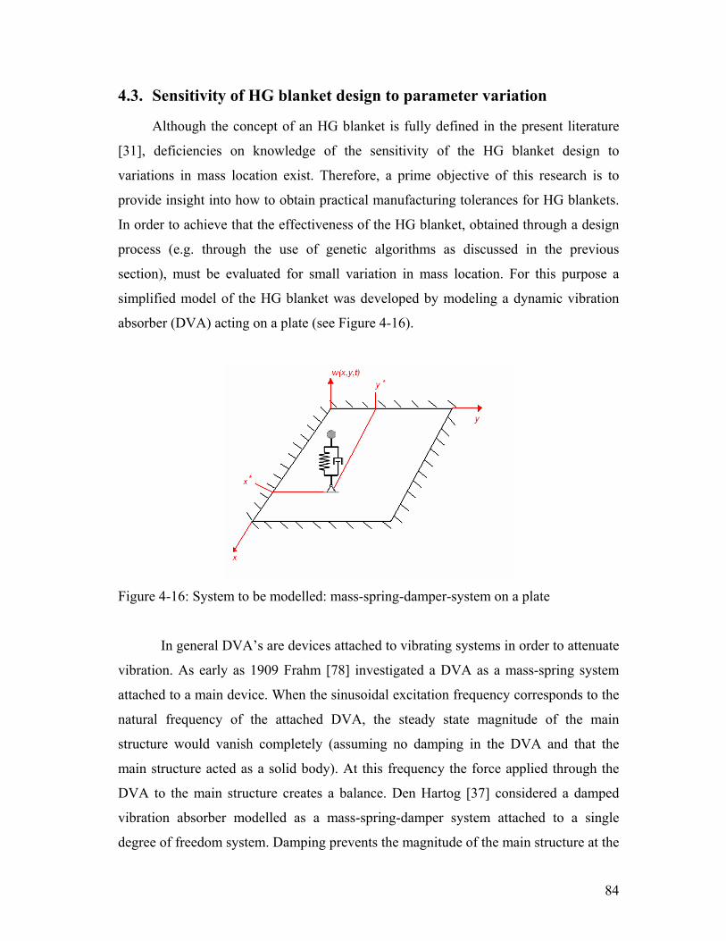
84

4.3. Sensitivity of HG blanket design to parameter variation

Although the concept of an HG blanket is fully defined in the present literature

[31], deficiencies on knowledge of the sensitivity of the HG blanket design to

variations in mass location exist. Therefore, a prime objective of this research is to

provide insight into how to obtain practical manufacturing tolerances for HG blankets.

In order to achieve that the effectiveness of the HG blanket, obtained through a design

process (e.g. through the use of genetic algorithms as discussed in the previous

section), must be evaluated for small variation in mass location. For this purpose a

simplified model of the HG blanket was developed by modeling a dynamic vibration

absorber (DVA) acting on a plate (see Figure 4-16).

Figure 4-16: System to be modelled: mass-spring-damper-system on a plate

In general DVA’s are devices attached to vibrating systems in order to attenuate

vibration. As early as 1909 Frahm [78] investigated a DVA as a mass-spring system

attached to a main device. When the sinusoidal excitation frequency corresponds to the

natural frequency of the attached DVA, the steady state magnitude of the main

structure would vanish completely (assuming no damping in the DVA and that the

main structure acted as a solid body). At this frequency the force applied through the

DVA to the main structure creates a balance. Den Hartog [37] considered a damped

vibration absorber modelled as a mass-spring-damper system attached to a single

degree of freedom system. Damping prevents the magnitude of the main structure at the

85

excitation frequency from becoming zero but decreases the sensitivity of the DVA due

to variations in the excitation frequency. Further research has been done to investigate

multi degree of freedom systems. Analytical and semi analytical methods have been

developed to design a DVA optimally. Since most structures are damped, Thompson

[36] showed an analytical way to tune the DVA parameters using the frequency locus

method. A relationship has been found describing the optimal constellation of these

values. Dayou and Brennan [79] focused on the positioning of DVAs on continuous

structures and developed a positioning method for multiple passive DVAs resulting in

attenuation close to active DVAs. In 2001 Jaquot [80] investigated a simply supported

plate with attached DVA and Jaquot’s model is similar to the model used in this study.

It is stated that attaching the DVA at a location which is driven by all modes dissipates

the energy of every mode in the entire frequency range of interest.

This section specifically presents the mathematical model of a clamped plate

with DVA on top. The sensitivity of HG blankets with respect to their effectiveness

with change in mass position is analyzed using one and two DVA’s. Finally the model

is validated experimentally using modal hammer tests.

4.3.1 Mathematical model This section presents the governing equations of DVAs acting on top of a

clamped plate used as a simplified model of HG blankets controlling a plate. The mass

inclusions inside the porous layer interact in reality at a certain distance away from

each other [35]. For simplification purposes, the masses are assumed to be uncoupled

masses acting as dynamic vibration absorbers with a certain effective stiffness and

damping value obtained experimentally [31]. The plate is modelled using Kirchhoff

plate theory. A Dirac-function [81] is used to distribute the force on an infinitesimal

small area. This means physically that a point force is applied. The equation of motion

for a plate and a DVA, including all assumptions, is given by 2

* *2 ( , ) ( ) ( )i twD w h p x y e F x x y y

tωρ δ δ∂

∆∆ + = ⋅ − ⋅ − −∂

, (4-1)

where x* and y* are the positions of the DVA with the DVA force F

and ( , , )p x y t representing the excitation, (generally due to turbulent boundary layer

86

noise in this application). The displacement w and velocity v of the plate can be written

respectively as

,( , , ) ( , ) i t

nm nmn m

w x y t C x y e ωφ= ⋅∑ , (4-2)

and

,

( , , )( , , ) ( , , )i tnm nm

n m

w x y tv x y t i C e i w x y tt

ωω φ ω∂= = = ⋅

∂ ∑ . (4-3)

The previous set of equations can then be rewritten to solve for the coefficients nmC

due to N DVAs:

{

2 211

112 212

12

2 2

11 11 11 12 11

12 11 22 22

1

0 0 00 00 0

00 0

( )(1 )

mnmn

mn

i i i

rs

CC

C

resonance matrix

f k i b Vexternalexcitation

ω ωω ω

ω ω

φ φ φ φ φ φφ φ φ φ

ω

φ φ

⎡ ⎤−⎛ ⎞⎢ ⎥− ⎜ ⎟⎢ ⎥⎜ ⎟⎢ ⎥ =⎜ ⎟⎢ ⎥⎜ ⎟⎢ ⎥⎝ ⎠⎢ ⎥−⎣ ⎦

−

− + −

L

O M

O O MM

M O O O

K K14444444244444443

L L

O O M

M O O O M

M O O O M

11

12

1

1

N

i

mnrs mn i

CC

C

DVA matrix

φ φ

=

⎡ ⎤⎛ ⎞⎢ ⎥⎜ ⎟⎢ ⎥⎜ ⎟⎢ ⎥⎜ ⎟⎢ ⎥⎜ ⎟⎢ ⎥⎝ ⎠⎢ ⎥⎣ ⎦

−

∑M

L L L144444424444443

(4-4)

The DVA-matrix has to be evaluated at the positions of the DVA. The effective

stiffness ki and damping bi are in reality given by the properties of the porous material

as well as by the interaction between the mass inclusion and the porous layer [35]. The

vector f contains a set of random complex numbers and the velocity of the plate is

computed 20 times, to simulate a random excitation which is similar in effect to a

turbulent boundary layer excitation [82].

4.3.2 Sensitivity study This section uses the previous model to discuss the sensitivity of the DVA in

terms of attenuation of the plate due to a change in mass position. In this chapter the

87

general definition of the sensitivity S is the change of the value c(u) with respect to a

parameter u and can be written as cSu∂

=∂

. In this study, u is the postion of the DVA

and c is the velocity. In the study with two DVA’s, u represents the position of these

DVA’s that are moved within the plate. The parameters for the clamped plate used

throughout the whole thesis are given in Table 2-1.

4.3.2.1. Sensitivity study on one DVA

To analyze the sensitivity of one dynamic vibration absorber acting on a plate, the

velocity spectrum in the frequency range of interest is computed. Thus, the best

position in terms of broad-band attenuation can be found by considering the attenuation

in a defined frequency range. The mass ratio of the DVA to the plate depends on the

frequency the DVA is tuned to. Therefore, the mass varies since the stiffness of the

foam is assumed to be constant. For example the mass ratio using one DVA is 0.1364

for the mass targeting the 1-1 mode and 0.02 for the mass targeting the 3-1 mode. The

criterion applied to target the 1-1 mode leads to the range from 70Hz to 200Hz is

calculated and plotted over the DVA positions marked with a “+”. The best position is

in the middle of the plate where the dominating mode has its highest magnitude, in this

case the 1-1 mode. The sensitivity, as expected, is strongly dependent on the dominant

mode shape. Figure 4-17 b) shows the magnitude of the gradient Sv

of the spatially

averaged velocity between each DVA position. The magnitude of the gradient is less in

the x-direction than in the y-direction since the plate is longer in the x-direction and

therefore the shorter the distance to the edge, the more sensitive is the DVA position.

The shape with lowest sensitivity can therefore be defined by an ellipse around the best

position and is dependent on the dimensions of the plate. Around the middle of the

plate the magnitude of the gradient is low and therefore the sensitivity is low as well.

In the following, the sensitivity with respect to the DVA position while targeting the

2-1, 1-2 and 3-1 mode is presented. The average velocity and the gradient of the

average velocity for the DVA targeting the 2-1 mode are plotted in Figure 4-18 a) and

b), respectively. The best position is where the 2-1 mode shape is at a maximum (anti-

node). Additionally, the positioning of the DVA targeting the 2-1 mode is more

88

sensitive than the positioning targeting the 1-1 mode. This is caused by the smaller area

that is provided by the 2-1 mode shape since the plate is divided into two halves by the

nodal line at x/Lx=0.5. As a result, the mass has to be positioned more accurately in

order to ensure that efficiency is not lost. It should be noted that Figure 4-18 a) is not

symmetric and this is caused by coupling with multiple modes (even though the 2-1

mode is clearly dominant) and the finite number of averages used to approximate the

turbulent boundary layer excitation.

Figure 4-17: Average velocity in the frequency range from 70Hz-200Hz; DVA targeting the 1-1 mode at 143Hz; crosses symbolize DVA positions on the plate. b) Magnitude of gradient of average velocity describing the change in magnitude (dB) among different DVA positions.

Figure 4-18: a) Average velocity in the frequency range from 180Hz-270Hz; DVA targeting the 2-1 mode at 225Hz; crosses symbolize DVA positions on the plate. b) Gradient of average velocity describing the change in magnitude (dB) among different DVA positions.

In Figure 4-19 a) the averaged velocity targeting the 1-2 mode is shown. As

would be expected, the plots for the 2-1 and 1-2 mode are similar.

Considering the DVA positions to target the 3-1 mode, Figure 4-20 a) presents

the average velocity. Again, the areas with the highest attenuation can be found on the

a) b)

a) b)

89

anti-node lines of the mode shape and the most effective locations for the DVA are

separated by a further nodal line. There is an increase in the sensitivity as seen in

Figure 4-20 b) due to the shorter wavelengths.

In conclusion, the design concept following the highest magnitude of the

targeting mode shape is sufficient and leads in all considered cases to the most efficient

position. Additionally, the sensitivity increases with the amount of nodal lines of the

dominating mode shape (i.e. in proportion to wavenumber).

Figure 4-19: a) Average velocity in the frequency range from 270Hz-340Hz; DVA targeting the 1-2 mode at 315Hz; crosses symbolize DVA positions on one quarter of the plate. b) Gradient of average velocity describing the change in magnitude (dB) among different DVA positions.

Figure 4-20: a) Average velocity in the frequency range from 320Hz-390Hz; DVA targeting the 3-1 mode at 348Hz; crosses symbolize DVA positions on one quarter of the plate. b) Gradient of average velocity describing the change in magnitude (dB) among different DVA positions.

4.3.2.2. Sensitivity study on two DVAs

In this study the sensitivity a combination of 48 DVA positions for each of two

DVAs was performed. Therefore 48*48 possibilities are evaluated. To describe the

sensitivity of a system with two DVAs, a way has to be found to compare and plot the

a) b)

a) b)

90

results. The positioning of two DVAs is based on the grid shown in Figure 4-21. Due to

the symmetry of the plate and the modes, one quarter of the plate is sufficient for the

placement of the DVAs. The plot principle can be described as “a picture in the

picture”. The first DVA has to be placed on the quarter of the plate (red dots on the big

plate in Figure 4-21). The green grid to the right of the 1st DVA represents the 48

possible positions on one quarter of the plate for the 2nd DVA. For example, the 1st

DVA is placed on the blue cross indicated in the figure by “Position of 1st DVA” and

the 2nd DVA is placed by the red cross. The red cross on the green grid describes the

DVA combination. Above this position the magnitude of the averaged velocity created

due to the action of both DVAs is plotted. This way a convenient plot can be created

including all details necessary for the DVA study.

Figure 4-21: Principle of DVA plot concerning different positions

In the following the combination with one DVA targeting the 1-1 mode at

143Hz and another one targeting the 3-1 mode at 348Hz will be considered. The 1-1

and 3-1 mode are the modes radiating most in the frequency range up to 500Hz and

therefore these modes should be attenuated.

91

Figure 4-22 shows the average velocity of two DVAs acting on a plate. The

regions with the lowest average velocity can be found in the middle of the whole plate,

where the first DVA acts most efficiently. The highest attenuation can be achieved if

each DVA is placed where the corresponding mode shape has its maxima.

Figure 4-22: Spatially averaged velocity (dB) with first DVA targeting the 1-1 mode

and second one targeting the 3-1 mode. Principle of plot is presented in Figure 4-21

Figure 4-23 shows the gradient of spatially averaged velocity (dB/DVA position

distance) with the first DVA targeting the 1-1 mode and the second one targeting the 3-

1 mode.

Generally, the sensitivity of the system is decreased compared to the sensitivity

with one DVA. If one DVA is placed at the best position, the sensitivity for the second

DVA is decreased. The results with two DVAs are therefore a combination of the

results given by the sensitivity analysis of the two DVAs performed separately.

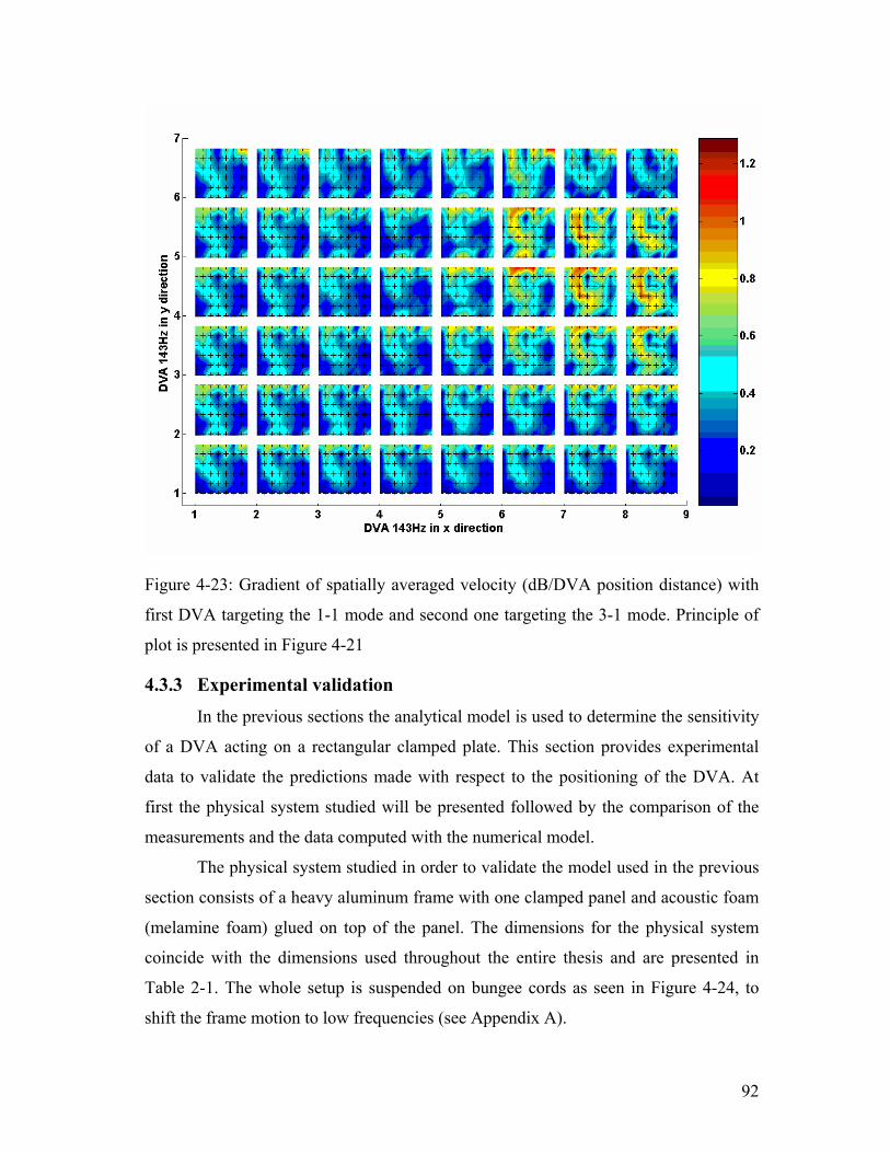
92

Figure 4-23: Gradient of spatially averaged velocity (dB/DVA position distance) with

first DVA targeting the 1-1 mode and second one targeting the 3-1 mode. Principle of

plot is presented in Figure 4-21

4.3.3 Experimental validation In the previous sections the analytical model is used to determine the sensitivity

of a DVA acting on a rectangular clamped plate. This section provides experimental

data to validate the predictions made with respect to the positioning of the DVA. At

first the physical system studied will be presented followed by the comparison of the

measurements and the data computed with the numerical model.

The physical system studied in order to validate the model used in the previous

section consists of a heavy aluminum frame with one clamped panel and acoustic foam

(melamine foam) glued on top of the panel. The dimensions for the physical system

coincide with the dimensions used throughout the entire thesis and are presented in

Table 2-1. The whole setup is suspended on bungee cords as seen in Figure 4-24, to

shift the frame motion to low frequencies (see Appendix A).

93

Figure 4-24: Experimental setup and grid for modal hammer excitement (ellipse)

Figure 4-25: DVA grid for experiments

To obtain an HG blanket acting as a DVA targeting the 1-1 mode of the clamped, a

rectangular mass (10mm x 10mm; 5.5g) was glued on top of the acoustic foam

(schematic is shown in Figure 4-26). In the measurements the mass is moved on a grid

presented in Figure 4-25. The DVA is only moved on one quarter of the plate since the

results for the remaining quarters are similar due to symmetry.

Figure 4-26: Schematic of HG blanket with mass glued on top of a porous layer

The excitation in the experiment is done with a point force at a constant

position. To match this excitation a point force is calculated for the model and the

transfer function is determined. The point force replaces the external excitation ( , )p x y

in Eq. (1) with ( ) ( )F FF x x y yδ δ⋅ − − , where Fx = 0.6Lx and Fy = 0.6Ly represent the

94

position on the plate. The position of the force is adapted to the position of the

accelerometer in the experiment. A random “boundary layer type” excitation was too

impractical to test, as it requires an enormous number of measurements, and therefore

this point force excitation was used to validate the model.

The maximum velocity of the measurement in a frequency range from 70Hz up

to 170Hz is plotted over the corresponding DVA position in Figure 4-27. The

corresponding prediction is shown in Figure 4-28. The tendency and observations made

in the prior section can also be applied to the results of the measurement. The best

position is found in the experiment close to the middle of the plate. An attenuation of

6dB is possible even if the DVA is adjusted slightly to a non-optimal position.

It should be noted that the results from the analytical model and the experiments

have not been scaled but the attenuation by the DVA is similar in theory and

experiment. In both cases an attenuation of about 6dB is achieved. In addition, the

tendency of the DVA position is equal and can be described by the dominating 1-1

mode shape.

Figure 4-27: Maximum velocity in the frequency range from 70Hz to 170Hz

determined by experiment

95

Figure 4-28: Maximum velocity in the frequency range from 70Hz to 170Hz

determined by the analytical model. DVA frequency adapted to 139Hz

In conclusion, a simple mathematical model is proposed to analyse the sensitivety

of a nominal optimized HG blanket. The model was verified and theory and the

experiment match well and the magnitude decay depending on the DVA position is

captured with a desired level of detail.

96

5. STUDY ON THE BEHAVIOR OF MASS INCLUSIONS

ADDED TO A PORO-ELASTIC LAYER This chapter presents a study of the behavior of the embedded masses inside the

poro-elastic media. A parametric analysis of mass inclusion behavior is presented,

probing both mass and stiffness variations inside the HG blanket. The parametric

analysis is conducted to tune the mass inclusions to the required HG blanket natural

frequencies. This can be done by either changing the mass or changing the stiffness.

The mass inclusion, acting like a distributed mass-spring-damper system, interacts with

a “finite volume” of the poro-elastic layer. This behaviour leads to HG blanket

characteristics such as the “footprint”, the “effective area” and the “mass interaction

distance”. An empherical approach is found and used to predict the natural frequencies

of different mass shapes embedded in porous media. An analytical approach is then

developed to describe the interaction of the mass inclusions with a poro-elastic layer by

simplifying a model for poro-elastic materials originally proposed by Biot [52] and

Allard [53] for low frequencies and by implementing basic elastomechanical concepts.

Both, the empherical as well as the analytical approach are compared to measurements

and shown to be accurate within 8% and 6%, respectively, over a range of porous

materials and mass shapes.

5.1. A study on the characteristic behavior of HG blankets

The objective of this section is to outline the characteristic behavior of mass

inclusions added to a layer of poro-elastic material. Furthermore, novel techniques for

predicting and tuning the resonance frequencies of the mass inclusions will be

presented.

5.1.1 FE model and experimental investigation This section presents the finite element (FE) model and experimental setup used

to analyze the HG blanket characteristics and the behavior of the mass inclusions. FE

results are used in cases where experimental results are difficult to obtain. The FE

model of the HG blanket is based on fundamental fluid, structural, and coupled fluid-

97

structural equations and was used in the previous chapters to develop the single-bay as

well as the multi-bay double panel system design tool.

5.1.1.1. FE model

The details of the finite element code used for this work are well presented in

Chapter 2 and therefore this section will only explain how the model was used for this

work.

The FE model of the HG blanket was used to analyze the interaction between the mass

and a block of foam (Melamine #1a in Table 5-1). Mass inclusions were placed at

single nodes in the FE mesh and the stress and displacement fields generated by the

masses could then be calculated. The foam block was excited with a uniform velocity

over its base, thus each node at the base was driven with a constant unit velocity.

Transfer functions between the input base velocity and the nodes corresponding to

mass inclusions could then be used to investigate the characteristics of the masses (such

as natural frequency and damping). In addition, the stress fields created by the masses

when excited could also be investigated.

Table 5-1: Model parameters of the FE model of an HG blanket.

Poro type Modulus of elasticity (N/m2) Density (kg/m3) Flow resistively (Ns/m4)

Melamine #1a

(white) 4.76 * 10^5 8.44 1.14 * 104

Melamine #2

(grey) 3.83 * 10^5 9.07 0.99 * 104

Polyurethane 1.05 * 10^5 28.98 1.3 * 104

Polyamide 3.0 * 10^5 7.86 35.3 * 104

5.1.1.2. Experimental Investigation

To study the fundamental behavior of a mass inclusion, block of porous

material with a single mass inclusion was used to determine the natural frequencies and

damping of the HG blanket. The test could then be repeated for various masses (various

shapes and weights). The mass inclusion was either glued on top of the porous block,

98

or inserted into the middle of the block after cutting the block in two pieces (half of the

depth). The two pieces were subsequently glued back together. Experimental studies

have shown minimal variations of the porous material properties using this technique.

An acoustic foam block (melamine#1 if not stated otherwise) was placed on top

of a shaker with the block glued to a stiff honeycomb platform (see Figure 5-1). An

accelerometer on top of the honeycomb platform and one on the mass inclusion

allowed the transfer function between the drive acceleration at the base and the

acceleration of the mass inclusion to be measured and natural frequency determined.

Figure 5-1 shows the data acquisition system with the HG blanket and the shaker.

Figure 5-1: Experimental setup to measure the natural frequencies of the mass inclusions inside the HG blanket. Shown is the data acquisition system (1), the HG blanket (2) and the shaker (3)

For the corroboration of the “effective area” approach (described below), three

additional porous media were used: a different type of melamine foam (Melamine #2),

polyurethane, and polyamide. The parameters for the four types of porous material

were measured and are presented in Table 5-2. The flow resistivity was measured using

the Ingard and Dear method [83] and the elasticity taken from a dynamic shaker test

[84]. The two melamine foams were acquired from two different companies and exhibit

similar, although not identical, properties. The polyurethane and the polyamide

parameters vary significantly from those of the melamine foam; the polyurethane has

high density while the polyamide has high flow resistivity. Only “typical” values are

99

defined since the properties of the foam can vary from sample to sample. The aim here

is to outline a universal approach to predicting and controlling mass inclusion behavior

in HG samples.

The material properties of a nominally identical acoustic foam produced in two

different batches can vary significantly and can also vary within a single batch even

within the same sheet. The five porous layers with melamine #1a utilized for results in

Table 5-2 (discussed in section 5.1.2.2) were all from the same large sheet of foam.

Melamine #1b comes from a different batch entirely. Provided experiments indicate

that the poro-elastic blocks cut from different batches can result in a five-fold increase

in the standard deviation of the natural frequencies as shown in Appendix C.

5.1.2 Parametric studies This chapter outlines vital HG blanket characteristics including the “footprint”,

the “mass interaction distance” and the “effective area” to allow prediction of mass

inclusion behavior.

The parametric studies of the HG blanket are performed to tune the mass

inclusions to the required natural frequency. There are two ways to tune a mass-spring

system: changing the mass or changing the stiffness. Since the poro-elastic layer acts as

a distributed spring, there are many parameters that can be varied to change the

effective stiffness, and these are investigated in detail and presented in the following

sections.

5.1.2.1. Tuning with varied mass

One way to tune the inclusion behavior is to change the mass of the inclusion. A

foam block (Melamine #1a) with dimensions 140x140x50 mm (length, width, and

thickness respectively), three inclusions, and an attached accelerometer were used. The

inclusions were individually glued on top of the porous block and tested sequentially.

Three different mass inclusions with the same surface shape and area were used. Mass

was varied from 11.7 g to 27.0 g. Figure 5-2 shows the measured transfer function

between the input acceleration of the base and output velocity of the three inclusions.

100

The resonance frequency follows accepted mass law since the natural frequencies were

proportional to the inverse square root of the mass.

Figure 5-2: Measured transfer function between the input acceleration of the base and output velocity of three different mass inclusions: 11.7g ( ), 18.7g ( ), 27g ( )

5.1.2.2. Tuning with varied stiffness

The stiffness of the HG blanket mass-spring-damper system is created when a

region of the porous media interacts with the mass inclusion. Tuning the mass

inclusions by varying the stiffness is a complicated process. To accurately predict

behavior, tuning with varied stiffness requires the definition of mass depth, a

“footprint,” “mass interaction distance,” and “effective area.”

Mass depth Varying mass depth is the simplest way to change the stiffness and thus the

natural frequency of a mass embedded in a layer of poro-elastic media like melamine

#1a. Figure 5-3 depicts the variation in resonant frequency of an 8g mass in a melamine

foam block (140×140×110mm) versus layer thickness. The resonant frequency of the

mass inclusion increases with decreasing depth x. To indicate the trend of the natural

frequency measurements, the solid line represents a curve fit through the data points

given as

6.04483.42nf x= + , (5-1)

101

Where the resonant frequency fn is inversely proportional to the square root of the mass

depth x converging at 83.42Hz. 83.42Hz is therefore the natural frequency that would

be expected for masses placed in very thick blocks of melamine.

Figure 5-3: Variation of resonant frequency of an 8 g mass in a melamine foam block as a function of the thickness of foam beneath the mass. Plotted are experimental measurements (+) and a curve fitted through measured data ( )

Kidner et. al [32] validated this measurement in a previous experiment with a

35×35×100mm melamine foam block. The analysis in the next section signifies that

Kidner et. al. used a porous block too small to take into account all stiffness effects.

Footprint When varying material stiffness, the concept of the “footprint” is vital. Since

the poro-elastic media acts as a distributed spring, a mass moving inside this media will

have a region of influence. The poro-elastic material directly adjacent to an inclusion

will move with the same displacement as the inclusion, but the displacement decreases

with increasing distance from the inclusion. Beyond a certain distance from the

inclusion the motion of the media becomes negligible. Therefore the inclusion can be

considered to have a finite region of influence, or footprint. Similarly the forces

generated by the inclusion only affect a finite region on the base of the poro-elastic

102

media. The forces are the largest directly underneath the inclusion, and increased

distance from the inclusion results in decreased forces. The footprint embodies the

volume of poro-elastic media that a mass inclusion influences and therefore also

delineates the stiffness. The definition of the footprint is dependent on what is

considered to be a “negligible” influence and in this chapter a working definition of

“footprint distance” is suggested. However, other definitions could also be used.

This section presents the basic concept of a footprint, defines the footprint

distance and investigates this concept in detail for a specific type of acoustic foam.

However, the footprint is likely to vary for different porous materials with varied

physical properties. Defining the footprint for a range of materials and for various poro

block thicknesses is a future endeavor and is beyond the scope of this document. The

aim is simply to provide a novel, systematic method to evaluate and define mass

inclusion interactions and performance.

To investigate the basic behavior of a HG blanket (Melamine #1a), the FE

model was run with a 20x8x8 uniform grid and simulated on a base plate that was

driven with a uniform velocity v in the z-direction (Figure 5-4(a)). Figure 5-4(b) shows

the operating deflection shape of the HG blanket when driven at resonance. This

operating deflection shape is a cut-out of the x-z plane of the blanket at the y-coordinate

corresponding to the mass position. In this example, the length and width of the block

of foam are 0.1 m and the thickness is approximately 0.05 m. The weight of the mass

inclusion is 5.6 g. The nodes of the FE model in its static position are noted with +’s,

and the displacements after moving the base plate are noted with x’s connected with

lines. A uniform velocity (and displacement) was applied to the base of the HG blanket.

The lowest row of static nodes has a constant distance to the displaced node lines since

they are directly attached to the base. As expected, the porous media provides less

motion with greater distance from the mass. One can see that the region of influence is

a non-uniform area around the mass inclusion, therefore the footprint is a non-uniform

volume considering that the operating deflection shape only shows the x-z plane of the

blanket. The key is to define and compute a horizontal distance to be able to account

for the interaction between the mass inclusions. This distance will be defined in the

next paragraph and denoted as “footprint distance”.

103

Figure 5-4: (a) Schematic of the HG blanket glued on a base plate moving with the velocity v. (b) An operating deflection shape of a layer of porous media with one mass inclusion (2-D). (c) Force at the base versus the distance x from the middle of the mass inclusion placed at the center of the 150x100x50 mm poro-elastic layer, or the numerical “footprint distance” computation

Similarly, Figure 5-4(c) shows a plot of the force at the base versus the

horizontal distance x from the mass inclusion that is placed at the center of a

140x140x90 mm (length, width and thickness respectively) poro-elastic layer. The plot

shows that the maximum force is directly below the mass and drops down to 5% of the

maximum force at a distance of approximately x=0.04 m. Therefore this distance can

be used as a working definition of the footprint distance.

In order to determine the footprint distance experimentally and to verify

mathematical results presented, a shaker experiment was chosen with the allocations

shown in Figure 5-1. A mass inclusion inside a very small porous block with length

and width much smaller than the footprint should experience lower stiffness than an

inclusion embedded inside a porous layer with infinite x and y dimensions. Increasing

the x and y dimensions of a small block of porous material with an inclusion should

lead to an increase in the natural frequency (i.e. more stiffness). This increase will

continue until the dimensions of the poro-block reach the volume in which the

a)

b) c)

104

inclusions interact, i.e. the footprint. Above this dimension, the natural frequency of the

mass inclusion should not change significantly. Figure 5-5(a) shows a schematic of this

concept. A block of melamine foam with a 5.6 g mass embedded in the center position

was used in the experimental design shown in Figure 5-1. Figure 5-5(b) shows the top

view of the porous block. As with the mathematical example, the dimensions are

140x140x91 mm (length, width, and thickness respectively). The measurement was

repeated while holding the thickness constant and cutting 10 mm off of each of the

sides. For the last measurement, only 5 mm was removed. Consequently, the

maximum distance X from the center of the mass inclusion to the side of the poro-block

is 7 cm. The distance X for the second measurement was 6 cm, and the remainder

followed the same trend. Figure 5-5(c) shows the experimentally determined natural

frequency versus the distance X. At X=0.07 m, the natural frequency is higher than the

one at X=0.015 m due to previously described stiffness effects. At X=0.04 m the natural

frequency of the embedded mass converges to 175 Hz, indicating that the natural

frequency does not increase significantly with enlargement of foam block dimensions

beyond this point. Thus, the footprint distance can be considered to be approximately

0.04 m for this case and is in agreement with the numerically computed footprint

distance described above.

Figure 5-5: (a) Schematic of the experimental “footprint distance” measurement, (b) Dimensions of the poro-layer, (c) Natural frequency versus the distance X of the experimental “footprint distance” measurement

Mass interaction distance When designing the HG blanket, inclusions interactions within a block of poro-

elastic material (like melamine #1a) are important. Two inclusions positioned a large

distance from each other within a porous layer will not interact, but two inclusions

a)

b) c)

105

directly next to each other will interact a great deal or even act as one large mass thus

have a large impact on the natural frequency of the HG blanket. The FE model of the

porous material presented in section 5.1.1.1 is used to investigate the distance when the

two mass inclusions are independent of each other, the “mass interaction distance.” A

foam block of dimensions 200x100x100 mm (length, width and thickness respectively)

with a 21x7x7 FE grid was used with two 5.6 g mass inclusions. The previous section

showed that the footprint distance for a 5.6 g inclusion in melamine foam is

approximately 0.04 m. Therefore one mass inclusion was positioned 0.04 m from the

side of the foam in a center-depth position and the second mass inclusion was

positioned 0.12 m away. In this configuration there are two identical natural

frequencies, one for each of the masses. However as the second mass is moved closer

to the first, the masses become coupled and the system must now be considered to have

two modes of vibration each with a different natural frequency (see Figure 5-6(a)). The

natural frequencies for the two modes were computed for various separation distances

and are presented in Figure 5-6(b).

Figure 5-6: (a) Schematic of numerical estimation of “mass interaction distance” and (b) FE results of natural frequencies of mass inclusions versus mass separation. Plotted is the mode of the first mass ( ), the mode of the second mass ( ), and the natural frequency of a single mass by itself ( )

One would expect that the inclusions stop interacting when the two footprints

no longer overlap and the two modal natural frequencies should converge to the

a)

b)

106

uncoupled natural frequencies. When the inclusions are very close together, the natural

frequency of one mode (masses moving out of phase) will tend to infinity, but the

second mode (masses moving in phase) will tend towards the natural frequency of a

single inclusion with twice the mass. This is bourne out in Figure 5-6(b) and it can be

seen that the masses stop interacting when they are 0.085 m away from each other i.e.

the mass interaction distance is roughly twice the footprint distance.

Effective area Masses embedded inside a porous layer interact with a certain volume of the

porous media. However, the footprint may change if the mass shape is changed. By

increasing the surface area of an inclusion (i.e. its projected area), it can be expected to

interact with a larger volume of the porous media. Therefore, the stiffness of the mass-

spring-damper system inside the HG blanket is expected to increase. A shaker

experiment, similar to the one shown in Figure 5-1, was used to measure the natural

frequencies of four inclusions with different shapes yet with similar mass. Figure 5-7(a)

shows a scheme of the HG blanket used in the shaker experiment with a mass glued on

the top of the porous block.

Table 5-2 displays the result of this experiment. The first two columns show the

mass and the projected area of the mass shapes. The ball, the beam, and the square have

significantly different projected areas. The projected area of the beam and the coin,

however, are roughly the same.

Table 5-2: Parameters and results from masses embedded in “melamine #1a”.

Mass

shape Weight (g)

Projected

area (m2)

Effective

area (m2)

Average mean

of nat.

frequency (Hz)

One-sided 90%

confidence

interval (Hz)

Theoretical nat.

frequency (Hz)

Ball 5.6 1.0*10-4 0.8*10-3 120.2 3.2 110.7

Coin 5.8 4.6*10-4 1.6*10-3 154.8 7.9 156.7

Beam 5.9 6.5*10-4 2.3*10-3 190.8 6.4 188.9

Square 5.9 18.0*10-4 4.0*10-3 240.2 8.7 246.1

107

Figure 5-7(b) presents the transfer functions between the input acceleration of

the base and output velocity of the four mass inclusions. Each measurement was

repeated five times using five different blocks of melamine foam #1a. The mean and

the one-sided confidence interval with a 90% probability are shown in Table 5-2. The

maximum standard deviation of the natural frequency is below 9 Hz for all of the mass

shapes (with a probability of 90%). As expected, the natural frequency increases when

the area of the masses is increased. Interestingly, although the areas of the beam and

the coin are very similar, the natural frequency of the coin is significantly lower than

the natural frequency of the beam. The results presented in Figure 5-7(b) and Table 5-2

indicates that the natural frequency does not simply change linearly with projected

area, but is also dependent on the shape of the inclusion.

Figure 5-7: (a) Schematic of the HG blanket experiments used for the “effective area” experiments, and (b) Natural frequencies of different mass shapes measured in shaker experiment. 5.6g ball ( ), 5.8g coin ( ), 5.8g beam ( ), 5.9g square ( )

As a first-order approximation, the stiffness of the mass inclusion can be

considered to change with an “effective area” that is defined in Figure 5-8(a) as a

perimeter a distance d away from the perimeter of the projected area. Consequently, the

“effective area” of a beam with the same projected area as a coin would result in a

significantly larger “effective area” and thus consequently in a larger footprint and

stiffness. This approximation assumes that the equivalent stiffness constant keq in the

a) b)

108

b)

mass-spring-damper system inside the HG blanket is a function of the effective area

a(d) and a porous material constant cporo (assumes a constant depth):

( )=eq porok a d c , (5-2)

Given the porous material constant cporo, the distance d and the mass weight m, one can

compute the natural frequency in Hz:

( )12

poron

a d cf

mπ= , (5-3)

Figure 5-8(b) shows the projected areas as a function of measured natural

frequencies (+’s connected with the solid line). The dashed line is the approximation of

the natural frequencies plotted as a function of effective area and using Eq.(5-3). A

family of curves with different d’s and cporo’s was plotted, and the dashed curve in

Figure 5-8(b) is the curve with the best fit through all measurements. The distance d

that best fits the data is used to calculate the effective areas listed in Table 5-2: and is

0.0105 m with cporo=3.9*106 N/m3.

Figure 5-8: (a) Schematic of the “effective area” concept and (b) comparison of the “projected” ( ) and the predicted “effective area” ( ) along with the measurements (+) of the ball (a), coin (b), beam (c) and square (d) versus frequency

To define this method as a universal predictive tool, a second type of melamine foam

block, melamine #1b, with different material properties was studied. The porous block

used in the previous experiments is denoted melamine #1a..

In order to predict the natural frequency as described in Eq. (5-3), one must

define the distance d and the material property cporo. The cporo depends on the material

a)

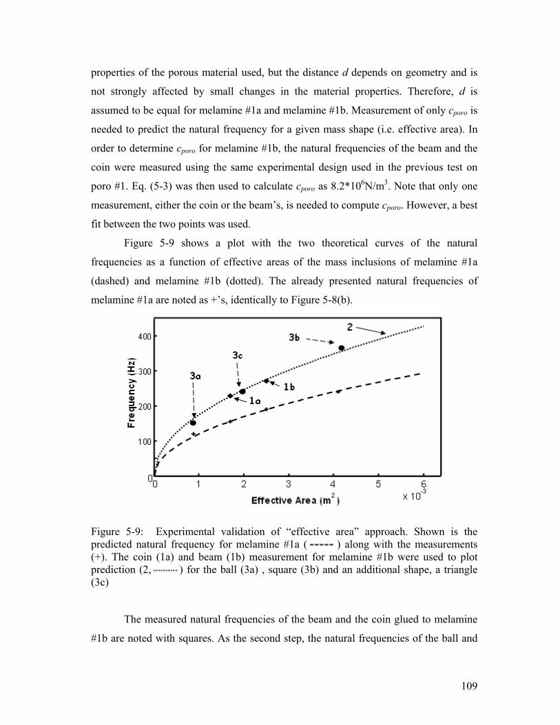
109

properties of the porous material used, but the distance d depends on geometry and is

not strongly affected by small changes in the material properties. Therefore, d is

assumed to be equal for melamine #1a and melamine #1b. Measurement of only cporo is

needed to predict the natural frequency for a given mass shape (i.e. effective area). In

order to determine cporo for melamine #1b, the natural frequencies of the beam and the

coin were measured using the same experimental design used in the previous test on

poro #1. Eq. (5-3) was then used to calculate cporo as 8.2*106N/m3. Note that only one

measurement, either the coin or the beam’s, is needed to compute cporo. However, a best

fit between the two points was used.

Figure 5-9 shows a plot with the two theoretical curves of the natural

frequencies as a function of effective areas of the mass inclusions of melamine #1a

(dashed) and melamine #1b (dotted). The already presented natural frequencies of

melamine #1a are noted as +’s, identically to Figure 5-8(b).

Figure 5-9: Experimental validation of “effective area” approach. Shown is the predicted natural frequency for melamine #1a ( ) along with the measurements (+). The coin (1a) and beam (1b) measurement for melamine #1b were used to plot prediction (2, ) for the ball (3a) , square (3b) and an additional shape, a triangle (3c)

The measured natural frequencies of the beam and the coin glued to melamine

#1b are noted with squares. As the second step, the natural frequencies of the ball and

110

the plate glued to melamine #1b were measured. Both lie on top of the predicted dotted

curve in Figure 5-9, noted as circles. The proposed formula works for porous media

with the four mass shapes: ball, coin, beam and plate. In addition a “new” mass shape:

a triangle with roughly the same weight as the other masses is introduced and the

“effective area” of the triangle lies between the “effective area” of the coin and the

beam. The natural frequency was measured and plotted in Figure 5-9 and is shown to

lie within 2% of the predicted value further validating this approach. The results are

summarized in Table 5-3.

Table 5-3: Parameters and results from masses embedded in “melamine #1b”.

Mass

shape Weight (g)

Projected area

(m2)

Effective area

(m2)

Nat. frequency

(Hz)

Theoretical nat.

frequency (Hz)

Ball 5.6 1.0*10-4 0.8*10-3 150 161.1

Coin 5.8 4.6*10-4 1.6*10-3 230 227.5

Beam 5.9 6.5*10-4 2.3*10-3 270 274.9

Square 5.9 18.0*10-4 4.0*10-3 370 358.1

Triangle 6.1 4.9*10-4 2.0*10-3 249 252.5

To prove that the “effective area” approach is not only valid for one type of

porous medium, three additional types of acoustic foam were used: melamine foam #2,

polyamide, and the polyurethane. These three types of porous media are some of the

most common materials used for interior noise control applications. Figure 5-10(1)

shows the comparison of the predicted and the experimental natural frequency of five

mass inclusions (a: ball, b: coin, c: triangle, d: beam, e: square plate) versus the

effective area for the melamine foam #2. All five mass shapes have the same weight of

approximately 6 g. The natural frequencies of the mass inclusions inside the melamine

foam remain close to the predicted curve with a maximum error of 5 Hz. Furthermore,

Figure 5-10 presents the validation for polyamide (2) and polyurethane (3). Both plots

show excellent correlation between theory and experiment. The experiments for

111

polyamide were executed carefully due to the compressibility of this porous media.

However, polyurethane use was in accordance with the use of melamine foam.

Figure 5-10: Comparison of theory ( ) and experiment (+) of “effective area” approach with (1) melamine foam, (2) polyamide, and (3) polyurethane. Measured are the natural frequencies of ball (a), coin (b), triangle (c), beam (d) and square (e).

In conclusion, the “effective area” approach was validated for three of the most

commonly used porous media: polyamide, polyurethane and melamine foam. The

results presented indicate a major step towards making the HG blankets a serviceable

treatment for interior-noise control applications. Using this approach, the natural

frequencies of the mass inclusions inside the HG blanket can be controlled entirely by

changing the shape of the inclusion. This allows all of the inclusions to be placed on

one layer, instead of varying the depth, and will make the blankets much easier to

manufacture. In addition, the use of the “effective area” theory is not limited to a

112

certain type of melamine but is applicable to a variety of foams. Most importantly the

proposed effective area approach, used to explain the natural frequency of different

mass shapes with constant embedded mass in porous media, has a maximum error of

8% for all the predictions made in this paper.

5.2. An analytical model for the interaction of mass inclusions with

the poro-elastic layer in heterogeneous (HG) blankets

The previous section introduced the “effective area approach” to determine the

resonant frequencies of a mass inclusion glued on top of a poro-elastic layer acting as

single dynamic vibration absorbers. The approach replaces the absorbers’ stiffness k

and determines the resonant frequencies of the dynamic vibration absorbers with

k mω = . This can be achieved by obtaining an effective stiffness provided by the

foam, which depends on the mass shape and poro-elastic material. Nevertheless, the

approach does not include all effects contributing to the resonant frequency of the

dynamic vibration absorber because the approach is too empirical. A novel approach

has thus been developed, which is analytically derived from the basic model for poro-

elastic materials proposed by Biot [52] and Allard [53] to backup and extend the

existing effective area approach. The proposed analytical model offers far more options

than the effective area approach. For example, the stress and displacement fields inside

the porous material can be calculated. Furthermore, the solution includes not only the

elastic properties of the material and influence of the mass shape but also the thickness

of the poro-elastic layer.

After presenting the derivation of the model and its two different modelling

strategies in the next section, the results and predictions of the model are shown with

special regard to the effective stiffness and the stress and displacement fields inside the

layer material of the HG blanket. An experimental validation of the effective stiffness

prediction is also included.

113

5.2.1 Mathematical model

5.2.1.1. Simplification of the Biot-Allard model for poro-elastic materials

Since the beginning of the 20th century, the mechanics of poro-elastic media

have been studied. Initial development came from the fields of geophysics and civil

engineering, leading to models for fluid-saturated soils. Later models were extended to

dynamics and the wave propagation inside the poro-elastic media, which not only

included soil-like materials but also air-saturated foams. Papers concerning the

development of models for fluid-saturated poro-elastic material have been published in

large quantities. An overview can be found in Ref. [85] and [86]. In this work, the

authors concentrate on a model which has originally been proposed by Biot in 1956

[52] and further developed by Allard [53] in 1993. This study assumes the material to

be an elastic frame with a fluid saturating inside. The constitutive equations for the

solid are written as follows when the summation convention is used:

223ij ij ij kk ijGG K pσ ε δ ε αδ⎛ ⎞= + − −⎜ ⎟

⎝ ⎠, (5-4)

where i,j = 1, 2, 3 (representing x, y, z), ijδ is the Kronecker symbol (1 for i = j, 0

otherwise), ijσ represents the components of the stress tensor and ijε represents the

strain tensor (given by the derivative of the displacement vector u). G is the shear

modulus of the material, K the bulk modulus andα accounts for the fact that the fluid

inside the poro-elastic material contributes to the normal stresses with its pressure p.

Shear stresses are not affected.

The first part of Eq. (5-4) (without ij pαδ− ) is the constitutive equation for a

linear elastic, isotropic material, while the additional term couples the fluid and the

frame phase. This coupling is the reason that it is difficult to model the poro-elastic

material properly and that the equations of motion (which can be found in Ref. [53])

get rather complicated.

In the previous chapters, the HG blanket was modelled using a FE scheme

proposed by Panneton and Atalla [57]. However, for HG blankets, the FE method

offers limited grid resolution and requires very high computation times. These

114

disadvantages, and the understanding that for a fast and efficient optimization of HG

blankets an easily manageable prediction of the effective stiffness is necessary, have

led to the conclusion that the Biot-Allard model has to be reasonably simplified until an

analytical and efficient solution can be obtained.

The assumption is made that the dynamic vibration absorber created by the

interaction of mass inclusions and foam layer does not couple to the acoustic field, and

its modelling, can be treated as a separate problem. This assumption has also been

made by Kidner et al. [32]. Furthermore, it is assumed that the air and the elastic frame

of the HG blanket are moving in phase at lower frequencies, and the air does not

present a large amount of stiffness to the poro-elastic material. The interaction between

fluid and frame is the main reason for energy dissipation and results in high frequency

noise reduction [53,87]. However, because the noise reduction nearly disappears at low

frequencies (only very thick foams still reduce low-frequency noise); the interaction is

hardly present in this state. It is therefore assumed that no energy dissipation is

provided by the interaction of fluid and frame.

Under these assumptions, the coupling between the fluid and the elastic solid phase of

the poro-elastic material might be present but is likely negligible for low frequencies.

Thus, the term ij pαδ− can then be neglected.

Under this condition, the constitutive equation of the poro-elastic material can be

reduced to:

223ij ij ij kkGG Kσ ε δ ε⎛ ⎞= + −⎜ ⎟

⎝ ⎠. (5-5)

This simplified form of the stress-strain relationship represents a linear-elastic,

isotropic material. It is not an accurate description of the HG blankets’ foam layer for

the whole frequency range since the bulk modulus of air is highly frequency dependent

and the interaction between the elastic solid frame and its saturating fluid is a central

characteristic of the poro-elastic medium. Yet, it is a valid assumption for the

considered low frequency range up to about 500 Hz.

The obtained linear elastic and isotropic constitutive equation (5-5) will be used

to develop a model to calculate the effective stiffness of the poro-elastic material and

will also explain certain other aspects of HG blankets. However, since the layer

115

material is now described as linear elastic, the following modelling steps can be

performed for all elastic (layer) materials. In order to highlight this generalization, the

layer of the HG blanket will be referred to in this section as an elastic layer.

5.2.1.2. Modelling of the elastic layer with added mass

In order to complete the modelling of the elastic layer, kinematical relationships

and equations of motion are necessary. However, for many applications it is assumed

that the stiffness for a static state is the same as for a dynamic state when the material is

considered linear-elastic and isotropic. The same assumption is made for the poro-

elastic layer of the HG blanket. The further modelling process will focus on a static

state. If a linear-elastic and isotropic material is assumed and volume forces (such as

weight, which is a small influence in foam and many other elastic materials due to the

low density) can be neglected, then the equilibrium conditions, the constitutive

equations and the kinematical relationships can be combined to the Lamé-Navier

equations [88],

( ) ( ) 2 0G Gλ + ∇ ∇ ⋅ + ∇ =u u . (5-6)

u represents the displacement vector, G is the shear modulus and λ is known as the first

Lamé constant, which can also be represented by other elastic constants as shown in

Table 5-4.

Although the material is now fully described, mass inclusions still have to be

modelled. The following modelling steps describe the HG blankets as mass inclusions

glued on top of the base layer instead of distributing them inside it, since this is very

convenient for the manufacturing process. In order to model a mass inhomogeneity on

top of a layer, a force acting in the z-direction (also denoted in this paper as “3-

direction”) is distributed over the mass shape’s cross-sectional area. Two modelling

strategies will be introduced in the next section. One with a constant force applied and

one with a constant displacement applied in 3-direction.

116

Figure 5-11: Schematic of the “real” HG blanket with a mass glued on top of a poro-elastic layer (a). Approximation with a force F distributed over the area of the mass leading to the pressure distribution p (b)

A direct analytical solution for the mentioned case is not known in literature,

but a solution in analytical form can be obtained by modifying a principal solution to

Eq. (5-6). This solution was discovered in the late 19th century by Boussinesq and

describes a single force oriented in the 3-direction acting on the top plane of a three

dimensional space, often called 3D “half-space” or “semi-infinite” space [88]. The

coordinate system used is presented in Figure 5-12. The position of the force F applied

at a point on top of the layer is described by the vector { }1 2 3, ,f f fx x x=fx while the

position of interest inside the material is described by the vector { }1 2 3, ,x x x=x .

Figure 5-12: The coordinate system for the “3D Halfspace” of the Boussinesq solution. The force F is applied at a point whose coordinates are described with the vector xf, while the actual position in the material is marked by x. The vector r = x - xf represents the difference of both vectors and has the magnitude R

x2

x3

x1

xf

x r

F

117

Table 5-4: Linear elastic, isotropic material constants and their expressions in terms of

modulus of elasticity E and Poisson´s ratio ν

Material constant Abbreviation Expression

Lamé´s constant λ ( )( )1 1 2Eνλ

ν ν=

+ −

Lamé´s constant µ ( )2 1EGµν

= =+

Shear modulus G ( )2 1EG µν

= =+

Bulk modulus K ( )3 1 2EKν

=−

The Boussinesq solution directly presents the displacement and stress field for

the whole body and includes the boundary conditions (e.g. the top plane of the 3D

“half-space” has to be stress-free in the 3-direction). The displacement in the 3-

direction created by the applied force in the 3-direction is

( )23 3

3 22(1 )4

fx xFuGR R

νπ

⎡ ⎤−⎢ ⎥= − +⎢ ⎥⎣ ⎦

) . (5-7)

F is the single force applied, G represents the shear modulus of the material and

ν is Poisson´s ratio, x3 is the actual position in the 3-direction inside the material (the

“z”-coordinate), and xf3 is the position of force application in the 3-direction while

R = fx - x (see Figure 5-12) is the distance from the applied force. Also, the normal

stress in the 3-direction is given by:

( )33 33 5

32

fF x xR

σπ

−= −) . (5-8)

The negative-sign is a result of the fact that compressive stresses are defined

negative, and that a force in the positive 3-direction creates a compressive normal stress

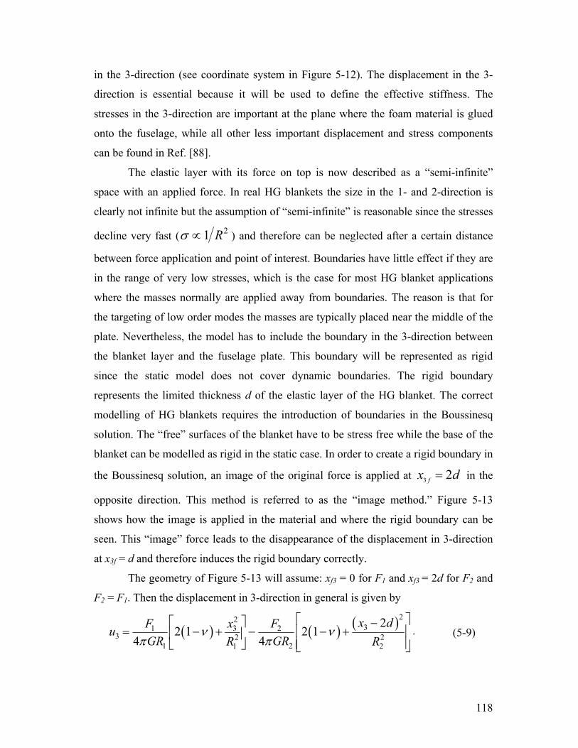
118

in the 3-direction (see coordinate system in Figure 5-12). The displacement in the 3-

direction is essential because it will be used to define the effective stiffness. The

stresses in the 3-direction are important at the plane where the foam material is glued

onto the fuselage, while all other less important displacement and stress components

can be found in Ref. [88].

The elastic layer with its force on top is now described as a “semi-infinite”

space with an applied force. In real HG blankets the size in the 1- and 2-direction is

clearly not infinite but the assumption of “semi-infinite” is reasonable since the stresses

decline very fast ( 21 Rσ ∝ ) and therefore can be neglected after a certain distance

between force application and point of interest. Boundaries have little effect if they are

in the range of very low stresses, which is the case for most HG blanket applications

where the masses normally are applied away from boundaries. The reason is that for

the targeting of low order modes the masses are typically placed near the middle of the

plate. Nevertheless, the model has to include the boundary in the 3-direction between

the blanket layer and the fuselage plate. This boundary will be represented as rigid

since the static model does not cover dynamic boundaries. The rigid boundary

represents the limited thickness d of the elastic layer of the HG blanket. The correct

modelling of HG blankets requires the introduction of boundaries in the Boussinesq

solution. The “free” surfaces of the blanket have to be stress free while the base of the

blanket can be modelled as rigid in the static case. In order to create a rigid boundary in

the Boussinesq solution, an image of the original force is applied at 3 2fx d= in the

opposite direction. This method is referred to as the “image method.” Figure 5-13

shows how the image is applied in the material and where the rigid boundary can be

seen. This “image” force leads to the disappearance of the displacement in 3-direction

at x3f = d and therefore induces the rigid boundary correctly.

The geometry of Figure 5-13 will assume: xf3 = 0 for F1 and xf3 = 2d for F2 and

F2 = F1. Then the displacement in 3-direction in general is given by

( ) ( ) ( )2231 3 2

3 2 21 21 2

22 1 2 1

4 4x dF x Fu

GR GRR Rν ν

π π

⎡ ⎤⎡ ⎤ −= − + − − +⎢ ⎥⎢ ⎥

⎢ ⎥⎣ ⎦ ⎣ ⎦. (5-9)

119

Where R1=|r1| and R2=|r2|. Therefore, the resulting 3-direction displacement at

the rigid boundary x3 = d is zero, regardless of the values of x1 and x2, and this satisfies

the boundary condition, As a consequence of the method, the solution gained by the

superposition of two opposing forces can only be used for 30 x d≤ ≤ . In direct

analogy to the approach made above, it is possible to show that all stress components

disappear at the rigid boundary when the image method is used, except the stresses in

3-direction, which double their value and are solely responsible for maintaining the

force balance. This behaviour must be expected for a correct representation of a rigid

boundary and is successfully implemented by using the image method.

Figure 5-13: The Image method leads to the introduction of a limited layer thickness d when 1 2F F=

The stress expression in general can be written analougus to the above shown

equation, such as:

Therefore, one disadvantage of the method is that the “image” force creates

stresses at the boundary at x3 = 0 disagreeing with the stress free condition as the stress

in that case is not zero. Nevertheless, this stress is negligible when the foam layer

thickness d is large enough, which is normally the case for HG blankets, where the

layer is thicker than 0.02 or 0.03m.

In order to describe the interaction between a mass inclusion and the blanket

material it is necessary to distribute the applied force over the cross-sectional

(projected) area of the mass. This is best described by a pressure p, which can be

( ) ( )3 31 3 2 3

3 5 51 2

3 3 22 2F x F x d

R Rσ

π π−

= − + . (5-10)

F1

F2

rigid boundary

x3 layer surface

image layer surface

d

dSemi-infinite

Semi-infinite r1

r2

x3

120

constant or a function of a coordinates x1 and x2. This pressure acts on the masses

cross-sectional area A in the 3-direction (see Figure 5-12). If the pressure p replaces the

single force F in Eq. (5-7) and Eq. (5-8) then the solution must be integrated over the

cross-sectional area of the mass to obtain the resulting displacement. Therefore, the

compliance V is defined as

this essentially allows the displacement in 3-direction to be expressed anywhere in

space as an integral over the surface area:

A “stress to force ratio” term is defined analogous to the compliance V, where

Thus, the stress in 3-direction can now be computed anywhere in space as

Numerical evaluation of displacement and stress in 3-direction

The above derived equations (5-12) and (5-14) are the analytical solutions for the

diaplacement and stress in 3-direction for any point inside the layer due to a distributed

pressure applied at the surface. In order to be able to solve these equations it is most

convenient to evaluate the integral numerically and the surface will therefore be

divided in i=1…I elements such that the numerical solution for the displacement can be

approximated as

( ) ( ) ( )2233 3

2 21 2

21 1( , ) 2 1 2 14 4

x du xVF Gd GdR R

ν νπ π

⎡ ⎤⎡ ⎤ −= = − + − − +⎢ ⎥⎢ ⎥

⎢ ⎥⎣ ⎦ ⎣ ⎦fx x

, (5-11)

3( ) ( , ) ( )A

u V p dA= ∫ f fx x x x . (5-12)

( ) ( )3 33 33

5 51 2

3 3 2( , )

2 2x x d

QF R Rσ

π π−

= = − +fx x . (5-13)

3( ) ( , ) ( )AQ p dAσ = ∫ f fx x x x . (5-14)

3( ) ( ) ( ) ii

u V p S=∑ if ifx x,x x , (5-15)

121

And the numerical solution for the stress is then:

where Si is the surface area of each element i and pi is the pressure applied on the

surface of each element Si.

Numerical evaluation of effective stiffness

The effect of one mass placed on top of the poro-elastic layer can be

approximated by a single degree of freedom dynamic vibration absorber with a spring

whose effective stiffness is provided by the elastic layer material. The spring stiffness

of a dynamic vibration absorber is assumed constant for the static and dynamic case

and can be written statically as a force over deviation of the spring: 3k F u= . In

direct analogy the effective stiffness calculated by the proposed model for the elastic

layer will be defined as an applied force over a displacement of the area of the

distributed force:

effavg

Fku

= . (5-17)

The elastic layer is assumed to be massless, thus, there is no need to define an

“effective mass” analougus to the “effective stiffness”. The force can then be

approximated by:

The resulting displacement is introduced by uavg using Eq. (5-7) such that:

3i ii

avg

u Su

A=∑

, (5-19)

where A represents the cross-sectional area of the mass.

The displacement and force at the surface are dependent and related to each

other by Eq. (5-11). Therefore, the displacement at all the elements can be decribed as a

vector u which is related to the pressures p through the I by I compliance matrix V

such that:

3( ) ( ) ( ) ii

Q p Sσ =∑ if ifx x,x x . (5-16)

i ii

F p S=∑ . (5-18)

122

u = Vp , (5-20)

where surface of the elastic layer under the mass is split up into i= 1...I small identical

rectangular elements with coordinates x1,i and x2,i and side lengths of 1x∆ and 2x∆ .

The displacement and pressure vectors, respectively, are then:

{ }1 2, ... Iu u u=u , { }1 2, ... Ip p p=p , (5-21)

where the compliance matrix includes the surface area of the rectangular elements such

that:

1 2( , )ij i jfV V x x x x= ∆ ∆ . (5-22)

for each matrix element ij. Since all evaluations of the model use Eq. (5-7) as a basis to

calculate the effective stiffness, a singularity of the equation, and therefore of the

diagonal matrix elements of the matrix V, occurs when the displacement has to be

evaluated at R = 0.

Essentially, the approach is to replace R = 0 (see Eq. (5-7)) of the singular elements iiV

in Eq. (5-22) with an effective radius to generate an equivalent displacement at the

center of the evaluation element due to the pressure over that element. The required

displacement due to a constant pressure over the element´s surface can be found

analytically by replacing the rectangular element with an equivalent circular element.

When the constant pressure p is applied on the element, 3u Eq. (5-7) for a general

element of area S can be written as

312 S

pu dsG Rν

π−

= ∫ . (5-23)

For the general case, R may be a complicated function of the location of the element ds.

However, if the area in question is a circle and the displacement in the center is

evaluated, one gets ds Rd drϕ= and the integral becomes

2

30 0

1 1 12 2

a

S

p pu ds Rd dr apG R G R G

πν ν νϕπ π− − −

= = =∫ ∫ ∫ , (5-24)

with the radius of the circular element a. The total force of the circular element Fel is

given by

123

2el

SF pds a pπ= =∫ . (5-25)

3u is then

3 21 1

el elau F F

G aGaν ν

ππ− −

= = . (5-26)

If the circular area is chosen to be the same as the rectangular elemental area

21 2a x xπ = ∆ ∆ , then 1 2a x x π= ∆ ∆ . Substituting this into the equation for 3u and

considering that 2

1 2elF p a p x xπ= = ∆ ∆ , leads to

1 23

1 2

1 1 12 2

2 4

elel

F p x xu F aaG G G x xν ν ν

π π ππ

− − − ∆ ∆= = =

∆ ∆.

(5-27)

By comparing this equation to Eq. (5-23), it can be seen that the displacement in

the center of the rectangular singular element can be approximated by assuming an

effective radius of

1 2

4effx xRπ

∆ ∆= . (5-28)

This effective radius is applied to all singular elements in the Eq. (5-11), where

the V matrix shown in (5-20), can be evaluated at R = 0. However, the assumption of

an effective radius is only valid for very small and square element sizes 1x∆ and 2x∆ ,

which has been considered for the computation of the results in this section.

In order to evaluate Eq. (5-17) to obtain an effective stiffness, two approaches

are proposed. One applies a constant pressure on the blanket surface across the

projected area of the mass using Eqs. (5-18) and (5-19) (strategy #1) and the other

specifies a constant displacement of the mass (stategy #2).

If a desired pressure distribution pdes is specified, in our case a constant

pressure, then Eq. (5-20) can be directly used to calculate the resultant displacements u

(this implies that the mass bends and is essentially limp). Once the pressure and

displacements under the mass are calculated an effective stiffness can be calculated

using Eqns. (5-17), (5-18) and (5-19).

124

If the force on top the elastic layer is applied evenly (strategy #1), the resulting

displacement of the mass’s cross-sectional area is not constant but shows

approximately a quadratic form, which can be seen in Figure 5-14.

Figure 5-14: Simulation of the displacement in 3-direction when a force of 1N is distributed over an area of 0.01m x 0.01m

For the second strategy, a displacement distribution desu is specified, which for

the case of constant displacement is simply an I length vector of velocities udes. In this

case the resulting pressures can be calculated as

1−= desp V u . (5-29)

Since V is not singular, p can easily be computed. Again, once the pressure and

displacement distributions are known then the effective stiffness can be calculated

using Eqns. (5-17), (5-18) and (5-19). It will be shown in the next section that both modelling strategies lead to nearly

the same results, when the prediction of the effective stiffness is considered.

125

5.2.2 Results With the help of the displacement field and stress field of the model, it is

possible to describe many properties of the HG blanket as well its behavior. These

results and a comparison of the two modelling strategies described in the last section

will be presented in the following sections, starting with the prediction of the effective

stiffness and leading to a description of the interaction between two masses on top of

an elastic layer.

5.2.2.1. Effective stiffness

In this section, the most important parameters influencing the effective stiffness

will be analyzed: The geometry of the mass and the thickness of the blanket layer. The

material parameters used in both strategies can be found in Table 5-5.

Table 5-5: Material values for evaluation of influence parameters on the effective stiffness

Parameter Value

Thickness of foam layer 0.051 m except when noted otherwise

Modulus of Elasticity E 380000 N m-2 except when noted otherwise

Poisson´s ratio ν 0.3

A higher cross-sectional area of the mass leads to the deformation of more layer

material. Therefore, the effective stiffness will increase since it is provided by the

interaction between the mass inhomogeneity and the blanket. This effect can be seen in

Figure 5-15.

The cross-sectional areas, natural frequencies, and effective stiffnesses for the

experimental validation of the model are presented in Table 5-6. Experiments have

been conducted using a shaker (similar to section 5.1.1.2) with a mass glued on top of a

poro-elastic layer to measure the transfer functions and natural frequencies of masses

with different shapes and areas. The experimental stiffness has been calculated from

the measured natural frequencies (deviation of ± 6 Hz) by evaluating the analogy of the

126

described setting with a single dynamic vibration absorber. The experiments were

conducted using melamine foam with the modulus of elasticity E = 320000 N m-2.

2 4 6 8

x 10-4

0

0.5

1

1.5

2x 10

4

area of mass shape [m2]

effe

ctiv

e st

iffne

ss [N

m-1

]

2 4 6 8

x 10-4

0

0.5

1

1.5

2x 10

4

area of mass shape [m2]

effe

ctiv

e st

iffne

ss [N

m-1

]

2 3 4

x 10-4

5000

6000

7000

8000

9000

10000

area of mass shape [m2]

effe

ctiv

e st

iffne

ss [N

m-1

]

Figure 5-15: Change of the effective stiffness with the area of the mass shape. A comparison between measurements ( ), predictions of the constant pressure ( ), and constant displacement ( ) model is included for all mass shapes. Part (a) shows the square mass shape, part (b) the rectangular shape with a side length ratio of 1:3, and part (c) the circular shape.

Both modelling strategies hardly diverge from each other and match

experiments well. Two significant conclusions can be drawn. The first conclusion is

that the stiffness does not linearly increase with the cross-sectional area A, as might be

suspected at first glance. Instead, the effective stiffness can be approximately described

as directly proportional to the square-root of the area for the presented area range

a) b)

c)

127

effk A∝ . The second conclusion is that the mass shape also has an influence on the

stiffness, even if the cross-sectional areas are identical. A circular shape leads to less

stiffness than a square shape, which has less stiffness than a rectangular shape with side

length ratios 1L a b= > . This is because the rectangular shape deforms more layer

material than the circular and square shapes. A more detailed study with the analytical

model leads to Figure 5-16(a), where the effective stiffness is calculated for a fixed

cross-sectional area while the side length ratio changes from 1 to 5.

Table 5-6: Comparison between experimental effective stiffness and the predictions of both modelling strategies for the effective stiffness of square, rectangular, and circular mass shapes with different cross-sectional areas

Cross-sectional area

[m2]

Measured stiffness

[N m-1]

Constant pressure strategy

[N m-1]

Constant displacement

strategy [N m-1]

Square shape

0.0001 3943 4652 4298

0.0002 5590 6409 6248

0.00035 7973 8501 8535

0.00046 10333 9789 9941

0.0009 16064 14196 14726

Rectangular shape (side length ratio 1 : 3)

0.0001 4067 5007 4580

0.0002 6222 6916 6669

0.00035 8447 9244 9123

0.0009 17023 15437 15783

Circular shape

0.0002 6000 5903 6064

0.00035 7869 7892 8299

0.00046 9416 9046 9521

128

1 2 3 4 55000

5250

5500

5750

6000

side length ratio a / b

effe

ctiv

e st

iffne

ss [N

m-1

]

0.03 0.06 0.09 0.12 0.15

4800

5000

5200

5400

thickness of elastic layer [m]

effe

ctiv

e st

iffne

ss [N

m-1

]

Figure 5-16: Part a) Dependence of the effective stiffness on the side length ratio a:b of an rectangular mass shape. Part b) Dependence of the effective stiffness on the thickness of the poro-elastic layer of the HG blanket. The cross-sectional area of the mass is 0.0001 m2. The evaluation is done with the constant displacement strategy.

The effective stiffness varies with the side length ratio a/b: The most elongated

mass piece leads to a nearly 20 percent higher stiffness than that of a square shaped

piece. This effect is very useful for tuning the mass inhomogeneity to a certain natural

frequency of the fuselage by simply varying the side length ratio while keeping its area

and mass constant. An additional benefit is the fact that the relationship between length

ratio and effective stiffness is approximately linear.

An important influence on the effective stiffness is the thickness of the poro-

elastic layer, which was based on experimental results in the previous section. The

proposed analytical model in this section takes the thickness of the poro-elastic layer

into account. Figure 5-16(b), shows that the effective stiffness increases with

decreasing layer thickness. This behavior is not unique to HG blankets, for example,

the stiffness of a rod with cross-sectional area A, length l and modulus of elasticity E is

defined as c EA l= . If the length l is reduced the stiffness increases. The more

material is available, the more deformation is possible. The poro-elastic layer act in

same way: When l is representative of its thickness while its other geometry and elastic

behavior is similar to EA, its effective stiffness will increase with decreasing thickness.

Figure 5-16(b) also shows that when the thickness passes a certain limit the stiffness

hardly changes anymore. This is because the mass only influences and deforms a finite

a) b)

129

volume of embedding material. If this volume is not limited by the boundaries, the

further increase of the thickness does not lead to the deformation of more material, thus

the effective stiffness remains the same. The effects of changing the thickness of the

elastic layer and the area of a square-shaped mass have been evaluated using the model

with the constant displacement strategy and plotted on different axes in Figure 5-17.

1 2 3 4 5 6 7 8

x 10-4

0.040.05

0.060.07

0.080.09

0.1

0.5

1

1.5

2

x 104

area of mass shape [m2]thickness of elastic layer [m]

effe

ctiv

e st

iffne

ss [N

m-1

]

Figure 5-17: Prediction of the effective stiffness based on the thickness of the poro-elastic layer and the area of a square-shaped mass

For a constant thickness, the dependence of the effective stiffness on the area

takes the same square root shape as in Figure 5-15, while for a constant area the

dependence on the thickness shows a relationship similar to Figure 5-16(b). Figure

5-17 shows that this is valid for all combinations and leads to the assumption that both

relationships can be superposed by multiplying the single influences. Furthermore, it

can be taken into account that the relationship between the side length ratio and the

effective stiffness is approximately linear, and that the effective stiffness is directly

proportional to the shear modulus G, and therefore also directly proportional to the

modulus of elasticity E. The combination of all these relationships has led to the

following formula for a rectangular mass inclusion:

130

( )( )0.122 1 0.03 1effk E d A L−= ⋅ ⋅ ⋅ + − , (5-30)

in which keff is the effective stiffness, d the thickness of the elastic layer, A the cross-

sectional area of the mass and L the side length ratio L a b= .

The formula has been developed iteratively, evaluating predictions of the model

with the constant displacement strategy for melamine foam with the material

parameters presented in Table 5-5. This simplified equation is not a perfectly precise

prediction, but nevertheless the relative deviation between effective stiffness

predictions of the model and the simplified equation does not exceed 11%. Since the

maximum error of 11% for the effective stiffness only leads to an error of about 5% in

the natural frequency of the mass inclusion, the error is acceptable for first steps in the

tuning process of HG blankets, as long as only a low frequency range of up to about

400 Hz is considered.

The usage of one single simplified equation for the prediction of the effective

stiffness can be beneficial, especially when an approach is chosen which follows in its

basic form Eq.(5-30), but allows the application to different materials by “free values”:

( )( )1 1effk E d A Lα βδ γ−= ⋅ ⋅ ⋅ ⋅ + − , (5-31)

while the notation is the same as in Eq. (5-30), the constants α, β, γ and δ represent the

new degrees of freedom which allow the application of the formula to be considered for

different materials. They can be evaluated by conducting experiments or from the

model. Eq. (5-31) is a direct consequence of the novel analytical model and could be

seen as its equivalent to the formerly developed effective area approach introduced in

section 5.1.2.2. While the effective area approach has been experimentally validated

using two degrees of freedom, the new approach has four, as the model includes more

influence parameters, e.g. the thickness of the blanket.

5.2.2.2. Mass interaction

Another huge advantage of the analytical model is that the complete

displacement and stress fields inside the layer can be predicted when distributed forces

are applied to simulate the mass inhomogeneities. While the displacement field can be

used to define and calculate the effective stiffness, the stress field gives insight to the

131

interaction between two (or more) masses which are applied onto the same layer. Since

it must be assumed that for an efficient tuning of HG blankets more than one mass may

be necessary it is important that this mass interaction be studied. Finite element

calculations were performed in section 5.1.2.2, which led to the conclusion that masses

interact with each other when placed close together and their interaction increases with

decreasing distance. This critical distance is denoted as “mass-interaction distance” and

will be the main subject of this section.

Since the analytical model represents a static solution to the description of the

poro-elastic layer, the dynamic behavior cannot be included. The dynamics of the poro-

elastic layer will certainly determine its stress field, but a qualitative approximation can

be done with the static model discussed in this work. The most important stress is the

normal stress in the 3-direction, for it determines the pressure on the fuselage (the

“rigid” boundary) and thus the effect of the mass-created dynamic vibration absorber

on the fuselage-plate. Therefore, only the stress in 3-direction will be shown here. Also,

the mass interaction effects directly follow from the interaction of the stress fields of

both masses.

The stress distribution for the two masses is shown in Figure 5-18. The masses

hardly interact with each other in the whole poro-elastic material, which can be seen

from the very small stress values (200 Pa or even just 100 Pa compared to the applied

stress of 104 Pa) in the middle plane between the masses. There is a small interaction

on the base plate, however, the stresses in between the masses are far smaller than the

stresses directly below the masses (less than 200 Pa to over 550 Pa). The exact values

should always be seen in comparison to the applied pressure, but a tendency is clearly

visible. If the distance between the two masses exceeds a certain value (in Figure 5-18,

0.08 m) the interaction will be negligible. This distance between the two masses is the

critical “mass-interaction distance” which has been conceptualized in section 5.1.2.2. If

the mass distance falls below the critical distance, the displacement and stress of one

mass affects the second mass leading e.g. to a change in the stiffness provided by the

second mass and vice versa. Figure 5-19 presents similar plots to Figure 5-18, but the

distance between the masses is only 0.03 m instead of 0.08 m.

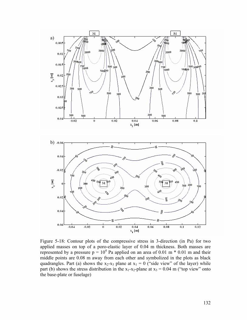
132

Figure 5-18: Contour plots of the compressive stress in 3-direction (in Pa) for two applied masses on top of a poro-elastic layer of 0.04 m thickness. Both masses are represented by a pressure p = 104 Pa applied on an area of 0.01 m * 0.01 m and their middle points are 0.08 m away from each other and symbolized in the plots as black quadrangles. Part (a) shows the x2-x3 plane at x1 = 0 (“side view” of the layer) while part (b) shows the stress distribution in the x1-x2-plane at x3 = 0.04 m (“top view” onto the base-plate or fuselage)

a)

b)

133

Figure 5-19: Contour plots of the compressive stress in 3-direction (in Pa) for two applied masses on top of a poro-elastic layer of 0.04 m thickness. Both masses are represented by a pressure p = 104 Pa applied on an area of 0.01 m * 0.01 m and their middle points are 0.03 m away from each other and symbolized in the plots as black quadrangles. Part (a) shows the x2-x3 plane at x1 = 0 (“side view” of the layer) while part (b) shows the stress distribution in the x1-x2-plane at x3 = 0.04 m (“top view” onto the base-plate or fuselage)

a)

b)

134

The stress fields created by the masses overlap, which leads to huge

interactions. On the base plate (at x3 = 0.04 m), the stresses are completely converged

to a single distribution so that the masses act as one. Qualitatively the stress distribution

for a long single mass looks alike.

In conclusion, both masses can be treated independent from each other when

the critical “mass-interaction distance” is exceeded. Furthermore, the stresses are

independent from the shear modulus (see Eq. (5-8)), indicating that the critical distance

is not affected by the material itself as long as the assumption, to model the HG blanket

as linear isotropic material, is valid. However, as soon as the masses are applied too

close to each other they will strongly interact leading, for example, to changes in the

effective stiffness.

135

6. EXPERIMENTS ON A GULFSTREAM FUSELAGE

SECTION This section gives an overview of the experiments conducted to demonstrate the

effectiveness of optimized HG blankets used to reduce the interior noise levels of civil

aircraft. These experiments are the final work of this thesis.

6.1. Preparation of fuselage measurements

The objective of these tests is to compare the sound transmitted through the

fuselage using two different passive noise control treatments (poro-elastic material vs.

HG blankets). A section of a Gulfstream fuselage formerly used in experiments with

Helmholtz resonators will be used for these experiments. Figure 6-1 shows the outside

of the Gulfstream section which is 10.7’ long with a diameter if 8.2’. Shown is also the

end cap on the front as well as on the back (not visible in the picture).

Figure 6-1: Section of a Gulfstream fuselage

Since the Gulfstream fuselage was used approximately 10 years ago for

Helmholtz resonator experiments, it had to be modified for the final HG blanket

measurements. Figure 6-2 shows the fuselage before (a) and after (b) the modifications.

The Helmholtz resonator experiments required an internal frame attached only to the

base to isolate the trim from the fuselage vibration. These internal frames were

removed. Additional screws on the fuselage were removed and holes due to corrosion

were filled out with paste. All windows were reinsulated with rubber mass. The

136

fuselage interior surface was grinded and cleaned. To decrease the floor vibration, the

mass of the floor was increased with an additional MDF board. In addition, the space

between the floor and the 1st layer of MDF was filled with fiberglass.

Figure 6-2: Gulfstream fuselage section before (a) and after (b) preparation for final measurements

Figure 6-3 presents the 2’’ thick melamine foam cut-outs that were be used to

build the HG blankets. All blocks were numbered using an indexing system of the

fuselage interior created with a CAD model.

Figure 6-3: Poro-elastic cut-outs

To measure the interior sound pressure level with the different experimental

configurations, a microphone array had to be designed. The array was designed to

accurately record frequencies up to 550Hz. Several possibilities were discussed and

a) b)

a)

Internal Frame

Additional MDF board on top of fiberglass layer

137

eventually the arrangement shown in Figure 6-4 a) was chosen. The main constraint

was to avoid aliasing, which means that the maximum distance between the

microphones and the trim panel had to be a half of the smallest wavelength. Because

the smallest wavelength is inversely proportional to the frequency, this constraint

would specify the upper wavelength limit. The array was mounted to the floor and was

moved to six different locations along the center line of the fuselage to capture the

whole cylindrical space. The array was turned 180 degrees after each measurement to

measure both sides of the fuselage interior. Figure 6-4 shows a picture of the

microphone array inside the Gulfstream fuselage.

Figure 6-4: Drawing of the microphone array, microphones marked with black dots (a) and real microphone array (b) for full scale fuselage measurement

Figure 6-5 presents the side view of the aircraft interior. The mounts (i) used to

connect the fuselage with the trim panel are neoprene bubble mounts, which are similar

to those used in the multi-bay double panel system (MPS) experiments in chapter 2.3

except they have a tripled maximum loading value. The trim panel used for this

experiment consists of four transparent, 5mm-thick, curved lexan sheets.

a) b)

138

Figure 6-5: Side view of fuselage interior.

These lexan sheets are connected with silicon on the sides as shown in Figure

6-5, with an additional narrow lexan sheet that connects the two sheets on the upper

center line of the fuselage as shown in Figure 6-6 (a). To reduce flanking, all holes in

the fuselage were sealed and a layer of melamine foam was positioned on the sides

(Figure 6-5, ii) of the trim panel and sealed with tape. In addition, the trim edges were

sealed as shown in Figure 6-6 (b).

Figure 6-6: Floor sealing (a) and trim connector sheet (b).

a) b)

i)

ii) ii)

ii)

139

Figure 6-7 presents a drawing of the experimental setup of the microphone

array (a, microphones marked with black dots, additional accelerometers marked with

red dots) and the real fuselage exterior (b) with a speaker to excite the fuselage and one

of three reference microphones positioned in front of the speaker.

Figure 6-7: Drawing of the experimental setup and the microphone array, microphones marked with black dots (a) accelerometers marked with red dots and picture of fuselage exterior with reference microphone and speaker (b)

Figure 6-8 presents the top view of the entire experimental setup including all

speaker and microphone array positions as well as the reference microphones. In

summary, the setup included three positions for a speaker (A to C Figure 6-8). The

speaker was emitting white noise with a frequency bandwidth from 0-1000Hz. It was

placed at a distance of 3ft away from the fuselage. To assure the repeatability of the

measurements, a reference microphone was set up at three positions synchronized with

the speaker (labeled Ref A to C in Figure 6-8). The reference microphone was placed at

a distance of 2ft from the speaker and 1ft from the fuselage.

The microphone array was moved along the center line and fixed at six different

positions (labeled I to VI in Figure 6-8). Furthermore, the microphone array was

alternately turned to the left and the right side of the fuselage (labeled L and R in

Figure 6-8). This setup enabled the sound pressure level throughout the fuselage

interior to be determined.

Reference Microphone

Speaker

b) a)

140

Figure 6-8: Top view of the experimental setup, showing the various positions of the speaker, the reference microphone and the array (I-VI R/L)

6.2. First fuselage measurements

This section presents the first measurements of the skin pocket vibration of the

Gulfstream fuselage and trim panel. The objective of these first measurements is to get

an idea of the skin pocket behavior. Five skin pocket groups were tested with different

configurations as shown in Figure 6-9. Three single skin pockets are tested as well as

two larger skin pocket groups with various hammer and accelerometer positions.

Looking at the light blue box in Figure 6-9, three frames divide the skin pocket group.

Note that this group is not touching the frames. Hence, although some skin pockets

look like they are subdivided by the frames, they actually act like one large skin pocket.

The same applies for the large skin pocket group highlighted in red in Figure 6-9.

Hammer positions are shown as “o’s” and accelerometer positions are represented by

“x’s.”

141

Figure 6-9: Picture of the interior of the Gulfstream section with the five skin pockets/ skin pocket groups used for the first measurements

Figure 6-10 shows the magnitude of the transfer mobility spectrum of the first

skin pocket observed i.e. it was excited with a modal hammer on a non-center position

with a measured response at the center of the panel. The first resonant frequency of the

skin pocket occurs around 330Hz.

Figure 6-10: Averaged mobility squared of 1st skin pocket measured at center position excited with modal hammer as shown in left picture

Figure 6-11, much like Figure 6-10, presents a plot of the magnitude of the

transfer mobility spectrum of the 2nd skin pocket excited with a modal hammer on a

non-center position with measured response at the center of the panel. The first modes

of this skin pocket are higher than those shown in the prior plot because the skin pocket

used for the measurement in Figure 6-11 has smaller dimensions.

142

Figure 6-11: Averaged mobility squared of 2nd skin pocket measured at center position excited with modal hammer as shown in left picture

Figure 6-12 shows the magnitude of the measured transfer mobility spectrum of

a large group of skin pockets excited with a modal hammer on a non-center position

with the accelerometer in the center of the panel. The first mode is below 200Hz, as

this skin pocket group has larger dimensions than the previous two skin pockets.

Figure 6-12: Averaged mobility squared of 1st group of skin pockets measured at center position excited with modal hammer as shown in left picture

Figure 6-13 presents two plots of measured transfer mobilities of the second

large group of skin pockets excited with a modal hammer on two non-center position (a

and b) with the accelerometer in the center of the panel. The responses of the two

curves are very similar at frequencies below 700Hz. This is expected because the

response to the same subset of skin pockets is measured at two different positions and

both attenuate most of the panel modes.

143

Figure 6-13: Averaged mobility squared of 2nd large group of skin pockets measured at center position excited with modal hammer on two positions as shown in left picture

The last measurement shown in Figure 6-14 presents a plot with three measured

transfer mobilities between panels with the accelerometer at the center of the third

small skin pocket. The skin pocket’s velocity is measured while exciting three

surrounding skin pockets; all three measurements look similar over the broadband.

Interpreting these results is quite complex because the three excited skin pockets (e.g.

the skin pockets with the hammer positions) are surrounded by different frames and

stringers. These three skin pockets also have different dimensions.

Figure 6-14: Averaged mobility squared of 3rd small panel measured at non-center position excited with modal hammer on three positions outside the panel, as shown in left picture

The above presented measurements show a wide range of “cut-on” frequencies

(i.e. 1st resonance frequency) of each skin pocket. They vary from 110Hz to frequencies

as high as 470Hz. Therefore, skin pockets with high cut-on frequencies should be

treated with different HG blankets than skin pockets with low cut-on frequencies. The

poro-elastic media damps out all skin pocket resonances above a certain frequency

(usually above 500Hz). Skin pockets with high cut-on frequencies only have a limited

144

number of low frequency modes that need to be controlled before the porous media

damps out those modes at higher frequencies. Thus, it was decided to measure each

skin pocket cut-on frequency individually in order to treat each skin pocket with its

own HG blanket design Figure 6-15 shows a histogram with the cut-on frequencies,

obtained with modal hammer tests, of each individual skin pocket. One can see that the

cut-on frequencies are distributed over a frequency range of 100-500Hz. However, it

appears that these cut-on frequencies occur in groups of certain small frequency

intervals, which show that the fuselage really consists of similar behaving skin pocket

groups. To simplify the HG blanket design process, the skin pockets were divided into

six groups with the natural frequencies of 127 Hz, 164 Hz, 263 Hz, 296 Hz, 347 Hz,

and 374 Hz.

Figure 6-15: Histogram of skin pocket cut-on frequencies

Figure 6-16 presents a plot with the measured spatially averaged squared

velocity of a trim panel over ten random points while the trim panel was excited at an

off-center position. This measurement was needed for the genetic algorithm design

tool (details in the next section), which is used to optimize the HG blanket. One can see

a significant amount of low frequency modes that need to be controlled with the HG

blankets.

145

100 200 300 400 500 600 700 800 900

-35

-30

-25

-20

-15

Frequency (Hz)

Spat

ially

ave

rage

d ve

loci

ty (d

B)

Figure 6-16: Measured spatially averaged squared velocity of a trim panel over ten random points and excited at an off-center position

The measurements shown in this section include three skin pockets and two

large skin pocket groups. All the skin pockets are very lightly damped. Skin pockets

with roughly the same dimensions act similarly even if surrounded by different BC’s.

For the full scale fuselage experiments, the design tool will take the different skin

pocket dimensions and BC’s into account when optimizing the HG blankets.

Furthermore, a modal hammer test with the trim panel revealed a significant amount of

modes to be controlled at low frequencies.

6.3. Procedure

This section briefly describes the procedure for the final HG blanket

optimization. The goal is to obtain the final optimized HG blanket design by modeling

the fuselage interior as realistically as possible and applying a genetic algorithm using

the design tool. The first step was to apply plane wave pressure excitation to the

fuselage as a more rigorous forcing function, as described in section 2.1.6. A genetic

algorithm was then applied to the MPS design tool. The genetic algorithm used is the

“Genetic Algorithm and Direct Search Toolbox” from MATLAB, as described in

section 4.2. The iterative optimization routine, also described in section 4.2, ran for a

certain configuration of the MPS and it was found that the MATLAB genetic

ii)

146

algorithm, when run for several weeks, converges to the results obtained with the

iterative method. The MPS experimental rig was designed similar to the fuselage

structure. Assumptions were made about the panel curvature as flat panels were used

for both fuselage and trim. The skin pockets inside the fuselage have various

dimensions which makes it difficult to capture all the dynamics of the fuselage using

the design tool. The MPS dimensions were changed to the most frequent dimensions of

skin pockets, frames and stringers inside the Gulfstream fuselage. Measurements of

fuselage and trim response have shown that the theoretical modes in the design tool

have to be adjusted to match the experiments due to the curvature of both panels as

well as the lexan material of the trim panel. The number of mass insertions has been

limited to four due to mass interaction distance limitations. The first test runs indicated

that the attenuation converged with four mass insertions while keeping the total mass

insertion weight constant. The mass has been unevenly distributed over the four mass

insertions and set as a constraint in the MATLAB toolbox. The fuselage and trim

modes vary throughout the fuselage section, thus, it was decided to run six different

cases (with different modes for fuselage and trim panel) on six machines. Figure 6-17

shows one of six possible HG blanket configurations.

Figure 6-17: One of six HG blanket designs (a) obtained with optimization routine and schematic of MPS (b).

a)

b)

147

Presented is the top view of the MPS with stars showing the mass positions (red

for top- and blue for bottom-nodes). The numbers inside the stars represent the mass of

the inclusions in grams. The genetic algorithm results give a good idea of the positions

and natural frequencies of the mass insertions inside the poro-elastic media.

The mass insertions of the final HG design are then tuned to the desired natural

frequencies using the “effective area” approach described in the previous chapter.

6.4. Comparison

This section discusses the final full scale fuselage measurements. The first part

of this section presents the comparison of the magnitude of the pressure ratios between

the 132 microphones inside the fuselage cabin with trim panel and the reference

microphone shown in Figure 6-8. Compared is the fuselage bare and treated with

melamine foam versus HG blankets. The resulted effect of the mass inclusions added to

the melamine foam was disappointing due to flanking transmission problems through

the windows, the floor or the doors. However, the second part of this section presents

measured spatially velocities of skin pockets, demonstrating that the HG blankets are

able to control the vibration of each skin pocket individually. Therefore, it is shown

that the fuselage structure can be controlled at low frequencies using HG blankets.

Figure 6-18 presents the magnitude of the pressure ratios between the 132

microphones inside the fuselage cabin (without trim panel) and the reference

microphone between the sound source and the fuselage from 30-530Hz. Compared is

the bare fuselage versus the porous media attached versus the HG blankets attached.

The melamine foam starts damping out the fuselage structure around 380Hz. Therefore,

all HG blankets target modes below 380Hz. Consequently, skin pockets with a cut-on

frequency above 380Hz were not treated with additional mass inclusions. The higher

the cut-on frequency of a skin pocket is, the fewer mass inclusions were added to the

melamine blocks. Effectively, a total mass of 3% of the fuselage weight was added to

the melamine foam in the form of mass inclusions (a maximum number of four mass

inclusions per block with mass varying from 3.5g to 19g). Unfortunately, no large

effect can be seen with the added mass inclusions.

148

Figure 6-18: Magnitude of the pressure ratio between the 132 microphones (inside the fuselage cabin without trim panel) and the reference microphone from 30-530Hz. Compared is the bare fuselage vs. porous media attached vs. HG blanket attached.

Figure 6-19 presents the magnitude of the pressure ratio between the 132

microphones inside the fuselage cabin (without trim panel) and the reference

microphone between the sound source and the fuselage from 30-1000Hz. Compared is

the bare fuselage versus the porous media attached versus the HG blanket attached. The

porous media controls the transmitted sound pressure through the fuselage by a

significant amount. Note the large number of modes over the bandwidth.

Figure 6-20 presents an a-weighted 1/12 octave band plot of the magnitude of

the pressure ratio between the 132 microphones inside the fuselage cabin (without trim

panel) and the reference microphone. Compared is the bare fuselage versus the porous

media attached versus the HG blanket attached. The porous media adds a significant

amount of damping to the skin pockets. No additional effect due to the mass inclusions

can be seen at low frequencies. The measured pressure ratios inside the cabin of the

porous media and the HG blanket are very similar.

149

Figure 6-19: Magnitude of the pressure ratio between the 132 microphones (inside the fuselage cabin without trim panel) and the reference microphone from -1000Hz. Compared is the bare fuselage vs. porous media attached vs. HG blanket attached.

Figure 6-20: Magnitude of the pressure ratio between the 132 microphones (inside the fuselage cabin without trim panel) and the reference microphone. Compared is the bare fuselage vs. porous media attached vs. HG blanket attached in 1/12 octave band (A-weighted).

150

Figure 6-21 presents the magnitude of the pressure ratio between the 132

microphones inside the fuselage cabin (with trim panel built in) and the reference

microphone between the sound source and the fuselage from 40-550Hz. Compared is

the bare fuselage versus the porous media versus the HG blanket attached. The

pressure ratio inside the cabin drops by a significant amount above 400Hz going from

“Bare” to “Poro” due to the porous media controlling the base structure at frequencies

above 380Hz. No additional effect can be seen from adding mass inclusions to the

melamine foam blocks, which makes sense as there was no effect due to the mass

inclusions without the trim panel attached to the fuselage structure.

Figure 6-21: Magnitude of the pressure ratio between the 132 microphones (inside the fuselage cabin with trim panel) and the reference microphone from 40-550Hz. Compared is the bare fuselage vs. porous media attached vs. HG blanket attached.

Figure 6-22 presents the magnitude of the pressure ratio between the 132

microphones inside the fuselage cabin (with trim panel built in) and the reference

microphone from 30-1000Hz. Compared is the bare fuselage versus the porous media

attached versus the HG blanket attached. The mounts above 400Hz are damped out due

to the porous media attached to the skin pockets. Comparing the porous media case to

the HG blanket case, the noise level inside the cabin is once more very similar.

151

Figure 6-22: Magnitude of the pressure ratio between the 132 microphones (inside the fuselage cabin with trim panel) and the reference microphone from 30-1000Hz. Compared is the bare fuselage vs. porous media attached vs. HG blanket attached.

Figure 6-23 shows an a-weighted 1/12 octave band plot of the magnitude of the

pressure ratio between the 132 microphones inside the fuselage cabin (with trim panel

built in) and the reference microphone. Compared is the bare fuselage versus the

porous media attached versus the HG blanket attached. One can see a small drop of the

magnitude of the pressure ratio around 320Hz going from the porous media to the HG

blanket. However, there is no proof that this is really due to the mass inclusions as the

rest of the pressure distribution is similar in both cases, with and without added mass

inclusions.

Figure 6-24 shows the measured spatially averaged velocity of a skin pocket

with a cut-on frequency of 125Hz in 1/12 octave band. Compared is the vibration of the

skin pocket with the porous block and with the HG blanket. The HG blanket has four

mass inclusions tuned to 125Hz, 170Hz, 240Hz and 340Hz. The mass inclusions cause

a significant drop in the skin pocket vibration at all targeted frequencies. Note that at

280Hz the HG blanket has a reverse effect by increasing the skin pocket vibration.

However, the HG blanket proved to be a very effective passive vibration control

treatment over the frequency band of 100Hz – 350Hz.

152

Figure 6-23: Magnitude of the pressure ratio between the 132 microphones (inside the fuselage cabin with trim panel) and the reference microphone. Compared is the bare fuselage vs. porous media attached vs. HG blanket attached in 1/12 octave band (A-weighted).

100 150 200 250 300 350 400

-8

-6

-4

-2

0

2

4

6

Frequency (Hz)

Spa

tially

ave

rage

d ve

loci

ty (d

B)

Poro

HG blanket2

Figure 6-24: Spatially averaged velocity of skin pocket with cut-on frequency of 125 in 1/12 octave band. Compared is the skin pocket with porous block and with HG blanket. HG blanket has four masses inclusions tuned to 125Hz, 170Hz, 240Hz and 340Hz.

To show that the HG blanket also works well for skin pockets with high cut-on

frequencies Figure 6-25 presents the spatially averaged velocity of a skin pocket with a

cut-on frequency of 330Hz in 1/12 octave band. Compared is the skin pocket with

porous block and with HG blanket. The HG blanket has one mass inclusion tuned to

153

340Hz. One can see that the vibration of the skin pocket is almost identical going from

the porous media to the HG blanket which proves the repeatability of the modal

hammer tests. However, the HG blanket causes a drop in velocity at the targeted

frequency. The reason for the attenuation being rather small compared to the previous

case is due to the mass of the inclusion. The mass of the inclusion used in this HG

blanket is only 4.5g because only light mass inclusions can be tuned to such high

frequencies with still having a reasonable area for the inclusion.

150 200 250 300 350 400

-5

0

5

10

Frequency (Hz)

Spa

tially

ave

rage

d ve

loci

ty(d

B)

PoroHG blanket

Figure 6-25: Spatially averaged velocity of skin pocket with cut-on frequency of 330Hz in 1/12 octave band. Compared is the skin pocket with porous block and with HG blanket. HG blanket has one mass inclusion tuned to 340Hz.

This section presented a full scale fuselage measurement of the sound pressure of

the cabin interior. The bare fuselage was measured and compared to the cases with

added melamine foam blocks and HG blankets attached to the skin pockets.

Unfortunately, no effect could be seen adding the mass inclusions to the porous layer

possibly due to flanking transmission problems. Flanking can be either caused through

the windows, the floor or the doors. However, the second part of this section presented

measured spatially averaged velocities of skin pockets with and without mass

inclusions added to the porous layer. It is shown that HG blankets are able to control

the vibration of each skin pocket individually by adding a total mass of 3% of the

fuselage mass distributed over all skin pockets.

154

7. CONCLUSIONS AND FUTURE WORK

7.1. Conclusions

In this thesis a numerical model has been developed that predicts the response

of a single-bay double panel system with sandwiched HG blanket and air cavity inside.

An impedance and mobility method approach (IMM) was used to couple the analytical

solutions of the fuselage and trim panel and air cavity with the FE model of the HG

blanket. This model was then validated experimentally and shown to accurately capture

the behavior of the double panel – HG blanket system.

The experimental and numerical results presented indicate that the analytical

model correctly predicts the experimental response of the double panel system with HG

blankets, and can be used as a design tool. It was also shown that it is possible to target

certain modes of the fuselage panel in a double panel system by tuning the masses

inside the HG blanket to the resonant frequencies of the fuselage panel. This results in

the reduction of the vibration levels of both the fuselage and trim panels, and a

reduction in the radiated sound field at low frequencies. It is also shown that the HG

blanket achieves this low frequency control while maintaining the high frequency

performance of the passive blankets (i.e. at frequencies above 500Hz).

An experimental investigation using the single bay DPS was presented,

attaching an HG blanket on both, the fuselage and the trim panel. These double HG

blanket measurements have shown promising results as the additional HG blanket on

the trim panel can be used to target modes that are tough to control from the fuselage

panel.

As a more rigorous model for an aircraft fuselage, the single-bay double panel

system was extended to include frames, stringer, mounts and four HG blanket. This

multi-bay double panel system was once again modeled using the IMM approach and

presented in chapter 3 of this thesis. A comparison between theory and experiment

showed a good match of the fuselage panel behavior and the predicted response of the

trim panel captured the main physical characteristics. However, the measured trim

panel results indicated problems in the repeatability of the experiments as the trim

panel has to be removed in order to change the HG blanket configuration.

155

Chapter 4 of this thesis presented a comparison of three different approaches to

the design of an HG blanket used to control the sound radiation from a double panel

system (random placement, modal design and best result in extensive search). An

extensive search of the solution space for a specific case of sound radiated from a DPS

with two mass HG blanket, was conducted and used to compare the different strategies.

The results showed that the best performing designs were substantially better than the

average “random” design with the best performer achieving 12.5dB attenuation (0-

500Hz), whereas the median performer achieved only 2.6dB attenuation in sound

radiation. The performance of the “modal designed” HG blanket was not much better

because the heavier of the two masses, used to attack the 1-1 mode, was positioned in

the middle of the fuselage panel, which turned out not to be the ideal position. In

addition the second mass in the model design case was used to target the 2-1 mode of

the fuselage panel. However, some of the modes of the fuselage panel, such as the 2-1

mode, are not all equally coupled to the trim panel and hence optimal control of the

fuselage panel does not lead to optimal control of the sound radiation.

Experimental results, based on the modal design method, show that the HG-blanket has

potential to significantly lower the vibration level of the fuselage panel at lower

frequencies while keeping the good performance of typical blanket treatments at

frequencies above 500Hz. The results also support the conclusions of the numerical

study: control of the fuselage panel by modal response does not lead to optimal results.

In addition, the comparison of theory and experiment for the presented “HG blanket

designs” has validated the design strategy.

The main conclusion from this work is that there is a strong need for

optimization routines such as genetic algorithms or iterative routines since optimal

performance is substantially better than the performance achieved using the other

simple design strategies. Therefore, a novel iterative routine for the HG blanket design

was introduced based on the sequential addition of massed in the blanket. After each

mass is added the optimal location/design for the next mass is found. When all of the

masses are added the algorithm then reassesses the design of the first mass and

continues until the design is converged. The iterative process was compared to the

results of an optimized HG blanket design obtained with the “Genetic Algorithm and

156

Direct Search Toolbox” from MATLAB. The optimized HG blankets obtained with the

above described algorithms are similar in results but vary significantly in their design

when increasing the solution space (e.g. mass positions and number of skin pockets)

due to the nonlinear relationship between design parameters and the cost function.

Thus, the solution space is not characterized by a single minimum but my multiple

minima and therefore gradient based algorithms were not considered in this work.

The design tool used to compare the optimization routines consisted of the

previously discussed DPS and MPS with sandwiched HG blanket and air cavity. For

this work the system was excited with an acoustic plane wave incident on the fuselage

panel. For the DPS the HG blanket was constrained to have four mass inclusions with a

given mass distribution to be placed on 50 positions. For the MPS the four HG blankets

were constrained to have two mass inclusions each with a given mass distribution to be

placed on 50 positions. The attenuation obtained with the HG blanket built with the

genetic algorithm as well as the iterative routine were similar. However, the iterative

routine managed to obtain its solution twice as fast as the genetic algorithm by

converging quickly after three runs in each of the two observed cases. Thus, the

iterative process has the potential to be even more computationally efficient when the

number of mass inclusions inside the HG blanket increases.

Furthermore, the sensitivity of HG blankets modeled of DVAs acting on a

rectangular clamped plate is investigated with respect to altering positioning of the

DVAs in order to analyze the performance of nominally optimal HG blankets. An

analytical model is derived using a Kirchhoff-plate and a DVA modeled as a mass-

spring-damper-system. The steady state response of the plate with DVA is calculated

and evaluated. To capture the effect of different excitations, the response due to

different excitation forces is calculated and averaged, thus simulating a random

“boundary layer type” excitation. The sensitivity of the placement of a DVA can be

predicted by a combination of the modes determining the velocity. Each mode shape

contributes at certain frequencies differently to the velocity of the plate. The analysis

done using the average velocity in the frequency range around the targeted frequency

reveals that the dominating mode shapes are indicators for sensitivity and the best

position. The highest magnitude of the mode shapes shows the best position. The slope

157

of the dominating mode shapes can be used to obtain the sensitivity of the positioning.

The sensitivity also depends on the amount of nodal lines. Every nodal line reduces the

area to place a DVA effectively and therefore increases the losses if the DVA is moved

from the best position. The model was also extended to include two DVAs and reveals

that the sensitivity of each DVA is fairly independent and therefore the results of a

single DVA can be used to describe the sensitivity of the positions for two DVAs.

Furthermore, the sensitivity of a system with more than one DVA decreases if one

DVA is placed at an optimal spot. In addition, the DVAs must be placed a certain

distance away from each other to avoid interaction caused by the foam. The model is

validated by experiments with different DVA positions. The results match well with the

theory and confirm the sensitivity analysis presented.

Chapter 5 presented a mathematical and experimental study of the behavior of

mass inclusions placed inside a poro-elastic media. The inclusions were shown to

interact with a finite volume of the poro-elastic media termed the “footprint” and it was

shown that this footprint impacted the tuning frequency of the mass inclusion and the

interaction distance between multiple masses. Inclusion mass and depth were shown to

alter the natural frequency of the inclusion and in addition it was also shown that both

the area and shape of the inclusion controlled the natural frequency by changing the

footprint.

A novel, empirical “effective area” approach to predict the natural frequency of

different mass shapes embedded in porous media was found and experimentally

verified for many different types of porous media, including melamine foam,

polyurethane, and polyamide. A maximum error of 8% existed for all the predictions

made.

By defining effective mass inclusion parameters, novel property control

methodologies for HG blanket materials were discovered that allow better control of

natural frequencies by controlling the mass, depth, area and shape of the inclusions. In

principle, inclusions of various shapes, placed on a single layer in the foam, can be

used to control a wide range of frequencies and this will make the blankets much easier

to manufacture.

158

Also in chapter 5 a new model for the interaction of mass inclusions with the

poro-elastic layer in heterogeneous (HG) blankets is presented. Since the previous

mentioned empirical effective area approach does not cover all parameters influencing

the interaction between masses and poro-elastic layer, the development of a more

sophisticated model to include more influence parameters was undertaken. This new

model was directly derived from the general constitutive equations for elastic media.

Basic elastomechanical solutions are implemented in the model making it

computationally far more effective than the finite element models. The model assumes

the system is essentially static and its limitations include a linear elastic and isotropic

constitutive relationship, which is critical for higher frequencies. However, the

analytical model covers all elastic materials and thus can be used in a far more

generalised way. The model is used to calculate the effective “dynamic vibration

absorber” stiffness created by the interaction between embedding material and the

added masses for low frequencies. The predictions are validated by experiments and

summarized in a simplified direct equation to calculate the effective stiffness, which

can be useful when dealing with experimental data in the HG blanket design process.

All known major influences on the effective stiffness of the elastic layer, namely the

material parameters, the mass shape and area, and the layer thickness are included in

the model. Furthermore, the model can also be used to predict the stress and

displacement fields in the elastic layer. Thus, the critical “mass-interaction distance”,

which is a necessary parameter in the HG blanket tuning and optimization process can

be computed. However, since the analytical model is static, it cannot be used to

investigate highly dynamic effects occurring when two masses are placed close to each

other leading to e.g. stiffness variations.

A full scale fuselage measurement of the cabin noise inside a Gulfsream

fuselage was presented in chapter 6 with and without an attached lexan-trim panel. The

bare fuselage was measured and compared to the cases with added melamine foam

blocks and HG blankets attached to the skin pockets. No significant effect could be

seen by adding the mass inclusions to the porous layer and this is probably due to

flanking transmission problems. It is assumed that the three possible flanking paths are

through the windows, the floor or the fuselage doors. However, modal hammer tests

159

measuring the vibration of individual skin pockets have shown the potential of the HG

blanket to control the vibration response of the fuselage structure at low frequencies by

a significant amount with only 3% (of the total fuselage mass) added to the 2’’ thick

melamine foam blocks. Overall, the HG blanket has shown potential for providing

good noise reduction over a wide frequency bandwidth.

7.2. Future work

As mentioned throughout this work, some issues are still unresolved or could be

further developed. The mathematical model for the single bay DPS was proved to be

accurate. However, the MPS measurements showed repeatability problems on the trim

side, thus the experimental rig could be further improved to have a good basis for a

comparison of theory and measurements. The double HG blanket measurements have

shown potential to further reduce the total HG blanket mass by controlling the trim

modes which are difficult to control with HG blankets attached to the fuselage side,

which is achieved by attaching an additional HG blanket directly on the trim. However,

this work needs some further investigation. The double HG blankets have not been

used in a full scale fuselage experiment with an additional HG blanket directly attached

to the trim panel.

Design and optimization strategies for HG blankets have been discussed in

chapter 4 where the mass inclusion position as well as the mass of the inclusions

(where a total mass was distributed over a limited number of inclusions) itself was

optimized. In order to further improve the HG blanket optimization, more parameters,

such as the poro-elastic material properties, the numbers of mass inclusions, as well as

the number of different mass distributions for the inclusions have to be taken into

account. In terms of the sensitivity analysis, future work should focus on variations in

the material parameters of the foam and plate boundary conditions which were not

considered in this work. Only by knowing these uncertainties can a reasonable

quantitative prediction of HG performance be made.

Mathematical and experimental approaches to describe the behavior of the mass

inclusions added to a porous layer have been presented. Yet, there is still a need to

160

analyze more types of poro-elastic material as well as fiberglass and other types of

damping material to fully define the HG blanket characteristics.

As for the analytical model of the mass-blanket interaction, future work is

needed concerning the study of the effects between masses in more detail, especially to

assess the influence of the mass shapes in this context. However, if this is the case, a

dynamic analytical or finite element model will have to be applied.

The full scale fuselage measurements have shown possible flanking issues.

Therefore, it is suggested to retake the measurements after treating the fuselage section

to reduce flanking path problems. Furthermore, in-flight measurements would provide

an opportunity to demonstrate the HG blankets potential to improve the interior noise

reduction at low frequencies in a more realistic environment.

Additional research is needed in order to investigate optimal manufacturing

processes for the HG blanket. The “effective area” approach allows the inclusions to be

placed in one level of the poro-elastic layer which makes the process easier. However,

there is still a need to investigate how applicable the HG blanket would be for aircrafts

with skin pockets of different dimensions throughout the fuselage. This could make the

HG blankets impractical.

Even though the HG blanket has shown its potential to reduce the vibration and

the noise transmitted from single and double panel partitions, it was only tested for

aircraft applications. More research needs to be done to test the HG blankets for

acoustic fields such as community noise, room acoustics and the interior noise control

of cars and trucks to fully explore the usage of the HG blankets in the market.

161

APPENDIX

A. Experimental measurement techniques - Improved validation of the DPS

This section presents some experimental techniques that improved the

experimental validation for the double panel system (DPS) in chapter 2. In the first

attempt to match the theory with the experiments of the DPS without HG blankets, the

major physics of the trim panel (at frequencies between 250Hz and 500Hz) were not

matched to a desired level of accuracy.

The inaccuracy on the experimental validation of the DPS without HG blankets

was most likely caused by three reasons. First, the design tool assumes absolutely no

frame motion. Different experimental approaches have been carried out in order to

reduce the frame motion and are presented in the next section. Second, the “trim panel”

has been removed from the excitation side and mounted on the receiver side. There is

always a change in the clamped BC due to imprecise torque on the bolts. This is further

analyzed by testing the repeatability of measuring the response of a clamped plate.

Third, the analytical solution for the cavity could be inaccurate. Improving the

accuracy of the single bay DPS experimental validation is vital because a more

complicated system will be used to optimize the HG blanket for the full scale fuselage

measurements, the multi-bay double panel system (MPS) discussed in chapter 2.3.

Finding mistakes in a DPS is a lot easier than finding them in a MPS, where the level

of complexity has increased significantly.

This section presents the process of solving problems due to frame motion and

repeatability of the experiments. After improving the experimental test rig, an

experimental validation is presented and shows that the desired level of accuracy is met

so that the analytical solution for the cavity is assumed to be correct.

A.1. Frame motion

In the introduction to this appendix, it was mentioned that one possible reason

for an inaccurate measurement could be the frame of the experimental rig moving in

phase with one of the plates. As an alternative experimental setup, three different cases

162

have been considered. First, the frame was mounted to a heavy worktable. Second, the

frame was placed on top of a piece of acoustic foam. Third, the frame was hung on a

crane.

In all three cases, the spatially averaged velocity of the clamped plate of a DPS at 25

measurement points has been compared to the spatially averaged velocity of the frame

at four measurement points. In order to measure the plate velocity, an accelerometer

was placed at an off-center position and a modal hammer was used to excite the plate at

all 25 points. To measure the frame velocity, an accelerometer was placed at four

positions on the frame. The clamped plate was excited by a modal hammer at the same

position the accelerometer was placed for the experimental validation in chapter 2. All

the frame motion measurements in this section are presented by using the 1.2mm plate,

which was used for the trim panel in the experimental validation throughout chapter 2.

Rigidly attached frame

In the design process of stopping the frame from moving, one alternative was to

bolt the frame to a heavier structure. In the first variation of the improved DPS

experiments, the frame was attached to a heavy worktable. Figure A-1 shows the

comparison of theory (red) vs. experiment (blue) of the spatially averaged velocity of a

clamped plate with the frame mounted to a heavy worktable (a). Furthermore, a picture

and the 3-D model (b) of the test case is presented in Figure A-1. The comparison of

the measurement and the design tool shows an additional peak and an additional zero

around 100Hz. In order to analyze if this was caused by the frame motion, the frame

motion itself was measured.

163

Figure A-1: (a) Comparison of theory vs. experiment of the spatially averaged velocity of a clamped plate with frame mounted to a heavy worktable, (b) picture of the experimental setup, (c) 3-D model of the experimental configuration

Figure A-2 shows the spatially averaged velocity of the clamped plate at 25

points compared to the spatially averaged velocity of the frame at four points (a), a

picture of the four accelerometer positions, and the position at which a point force was

applied (b).

Figure A-2: (a) Measured plate and frame spatially averaged velocity a clamped plate with frame mounted on a heavy worktable, (b) Picture of experimental setup measuring frame motion on four points while hammering on an off center position

0 200 400 600 800 1000-100

-80

-60

-40

-20

0

20

Frequency (Hz)

Spa

tially

ave

rage

d ve

loci

ty (d

B)

Effect of Frame Motion on Plates in DPS

FrameFuselage

a) b)accelerometer

200 300 400 500 600 700-50

-45

-40

-35

-30

-25

-20

-15

-10

-5

0

Frequency (Hz)

Spa

tially

ave

rage

d ve

loci

ty (d

B)

TheoryExperiment

accelerometer a) b)

c)

164

The result in Figure A-2 shows that the additional peak shown in Figure A-1 is

caused by the frame moving in phase with the clamped plate around 100Hz, which

shows two additional facts. First, the frame motion can be measured and compared to

the plate motion with the proposed setup of four measurement points on the frame.

Therefore, for the next experimental setups, the same experimental method will be used

in order to analyze the frame motion. Second, the frame motion at frequencies above

the lowest resonant frequency is much less than the motion of the plate and can be

neglected.

Frame on top of foam

Another method to reduce the frame motion is to damp it out by setting the

frame on top of acoustic foam. In this experiment, 2’’ thick melamine foam was used.

Figure A-3 shows the spatially averaged velocity of the clamped plate at 25 points

compared to that of the frame at four points (a), a picture of the four accelerometer

positions, and the position at which a point force was applied (b).

Figure A-3: (a) Measured plate and frame spatially averaged velocity a clamped plate with frame placed on top of a 2’’ thick piece of melamine foam, (b) picture of experimental setup measuring frame motion on four points while hammering on an off-center position

The results in Figure A-3 are an improvement compared to those found with the

frame mounted to the worktable, as presented in the previous section. At 150Hz, the

100 200 300 400 500 600 700 800 900

-90

-80

-70

-60

-50

-40

-30

-20

-10

0

Frequency (Hz)

Spa

tially

ave

rage

d ve

loci

ty (d

B)

Frame Motion DPS- Fuselage SideDPS - 1.2mm Fuselage (Experiment)

accelerometerb)a)

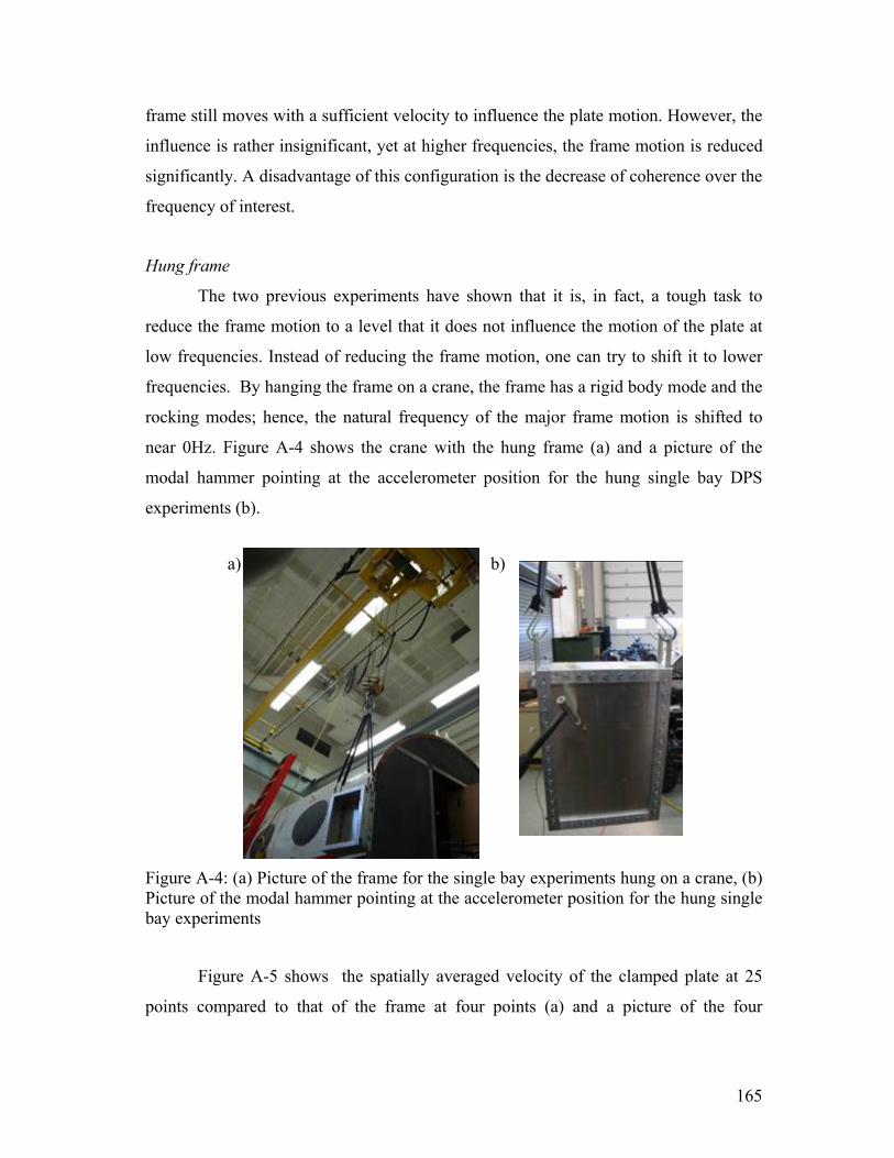
165

frame still moves with a sufficient velocity to influence the plate motion. However, the

influence is rather insignificant, yet at higher frequencies, the frame motion is reduced

significantly. A disadvantage of this configuration is the decrease of coherence over the

frequency of interest.

Hung frame

The two previous experiments have shown that it is, in fact, a tough task to

reduce the frame motion to a level that it does not influence the motion of the plate at

low frequencies. Instead of reducing the frame motion, one can try to shift it to lower

frequencies. By hanging the frame on a crane, the frame has a rigid body mode and the

rocking modes; hence, the natural frequency of the major frame motion is shifted to

near 0Hz. Figure A-4 shows the crane with the hung frame (a) and a picture of the

modal hammer pointing at the accelerometer position for the hung single bay DPS

experiments (b).

Figure A-4: (a) Picture of the frame for the single bay experiments hung on a crane, (b) Picture of the modal hammer pointing at the accelerometer position for the hung single bay experiments

Figure A-5 shows the spatially averaged velocity of the clamped plate at 25

points compared to that of the frame at four points (a) and a picture of the four

a) b)

166

accelerometer positions (red) and the position at which a point force was applied (light

blue).

Figure A-5: (a) Measured plate and frame spatially averaged velocity a clamped plate with hung on a crane, (b) picture of experimental setup measuring frame motion on four points while hammering on an off center position

The results in Figure A-5 show an additional improvement on reducing the

frame motion of the clamped plate measurements for the single bay DPS

measurements. The velocity at lower frequencies is small enough to not cause any

major problems in experimentally validating the design tool for the DPS.

In conclusion, three different experimental setups for the DPS were tested and

the frame motion was compared to the plate motion in each case. From all three cases,

it could be seen that the frame motion was only significant at frequencies lower than

the fundamental frequency of the plate. Mounting the frame to a worktable has shown a

significant frame motion below the first resonance of the plate, due to tension between

frame and plate. Placing the frame on top of poro- elastic material has damped out the

frame motion enough to not be significant. Hanging the frame of the DPS has shifted

the modes of the frame to lower frequencies. The reduction of the frame motion in the

last two cases is satisfactory. Therefore, the single and multi bay double panel system

measurements will all be taken by either placing the frame on top of poro-elastic

material or by hanging the frame.

0 200 400 600 800 1000-100

-90

-80

-70

-60

-50

-40

-30

-20

-10

0

Frequency (Hz)

Spa

tially

ave

rage

d ve

loci

ty (d

B)

DPS - 1.2mm Fuselage (Experiment)Frame Motion DPS- Fuselage Side b)

accelerometera)

167

A.2. Improved preciseness of torque on frame bolts After analyzing the frame motion, the second point to check was the

repeatability of the DPS measurements. The DPS consists of two clamped plates. The

responses of both panels are measured and verified just by themselves before they are

validated in the DPS. The response of a single plate was almost identical in theory and

experiment as shown in section 2.2.1. In order to build the DPS, one of the two plates

has to be removed from the source side and bolted to the receiving side. In an ideal

scenario, where the cavity in between the two panels is modeled correctly as well as the

coupling between the two panels, the DPS system consequently would match in theory

and experiment. This would only be the case if removing the plate from the source to

the receiving side would not have any effect, seeing how the frame motion was reduced

significantly in the previous section. One way to check the repeatability is to match the

DPS measurements with the design tool predictions and then change the source panel

to the receiving panel and the receiving panel to the source panel (in other words: swap

the DPS around) and see if theory and experimental results still match without

changing the aspect ratio of in the design tool. This has been done, and it turned out

that this was not the case; hence, the repeatability of this experiment had to be

improved. In order to analyze the repeatability of the experiment, the simplest

experimental configuration was chosen: a clamped plate by itself. A clamped plate was

measured, removed and bolted back to the frame, and it could be seen that the natural

frequency of these two measurements were significantly different. The assumed reason

for this was a lack in preciseness of the torque on the bolts. In order to solve this

problem, a torque wrench was used.

Figure A-6 shows the spatially averaged velocity of the clamped plate (a) using

a manual torque wrench (blue), an electric torque wrench (red), and no torque wrench

at all (black). An electric drill with torque setting is shown in Figure A-6 (b) and was

found to be accurate enough to replace the manual torque wrench. The blue and red

lines are almost identical. The black line, in comparison, has some significant variation.

168

Figure A-6: (a) Comparison between a clamped plated measurement of the spatially averaged velocity using with (red and blue line) and without (black line) using a torque wrench to mount the plate to the frame, (b) picture of used electronic torque wrench

Figure A-6 points out two important facts. First, the preciseness of the torque on

the frame bolts could be increased by using a torque wrench. Second, there is no

difference in the performance of the DPS between using a manual or electric drill for

bolting the plate to the frame. The only difference is, when using a manual torque

wrench, one can read the torque off the display; with an electric drill, one can only set

the torque to an unspecified level. Seeing how in our case there is no need of knowing

the exact torque, the drill was used, because it is easier and faster.

A.3. Improved validation for DPS After solving the frame motion and repeatability problems in the previous two sections,

the experimental validation of the DPS has been redone. The experimental validation

before and after improving the DPS are compared (trim panel) in this section.

Figure A-7 shows the experimental validation of the receiving side of the old

DPS (a). This validation is compared to the experimental validation with the improved

experimental techniques (b). The experimental validation in (a) shows that the

dynamics of the trim panel were captured correctly at frequencies below the first four

100 200 300 400 500 600 700 800 900

-40

-35

-30

-25

-20

-15

-10

-5

0

5

Frequency (Hz)

Spa

tially

ave

rage

d ve

loci

ty (d

B)

0.8mm Plate - Torque Wrench 1st try0.8mm Plate - Torque Wrench 2st try0.8mm Plate - Without Torque Wrench

a) b)

169

modes. After that frequency, one can see the correct trends, but it is hard to tell which

modes in the experiment belong to the predicted modes. The new experimental

validation (b) captures all the modes at the frequency of interest. Note that the

discrepancies at low frequencies are most likely caused by the frame motion as the

frame is not completely stopped from moving.

Figure A-7: Comparison of the experimental validation of a single bay DPS on the receiver side (trim), excited at a non center position (a) with and (b) without new improvements

In conclusion, three problems have been considered in order to improve the

experimental validation of the DPS. First, the frame motion of the experimental test rig

was suspected to influence the plate motion of the DPS plates. Second, the repeatability

of the measurements was doubted. Third, the equations for the cavity, coupling the two

plates, were assumed to be another source of error. The frame motion was reduced by

placing the frame on top of poro-elastic media as well as by hanging the DPS. The

repeatability of the DPS measurement was increased by using a torque wrench, which

improved the preciseness of the bolts. An experimental validation with the new

improvements was compared to the validation obtained before the improvements. The

dynamics of the trim panel are now all captured in the frequency of interest. Therefore,

there is no need in further analyzing the cavity model for the DPS.

a) b)

170

B. HG interface Going from the FE model to the fully coupled double panel system (DPS)

presented in chapter 2, it became difficult to use the design tool by just running the

code. In order to clearly lay out the code, the HG interface was developed. The

software is composed by several graphical user interfaces (GUIs) that are front ends for

the original FE code for the poro-elastic media and other utility functions for the

performance evaluation of dynamic systems composed by plates, poro-elastic media

and cavity.

The main function loads the default parameters, defines some global variables

and runs the main interface. All routines are working with a global structure which

contains all the variables that the user can change operating on GUIs.

Figure B-1 shows the main HG interface as it appears by running the main

program. Plate and poro-elastic media configurations, parameters and grid size can be

chosen dependent or independent from each other. Also, the frequency range for the

transfer function plots can be chosen from this interface. Furthermore, there is the

option to save and load certain parameter configurations and material properties.

Figure B-1: HG Interface developed for a clearly laid out usage of the developed code for the coupled DPS

171

Different configurations for the various physics can be chosen as shown in

Figure B-2. This is a useful feature when analyzing and debugging the program. Also,

for the experimental validation, it is useful to be able to just compute the response of

certain configurations first before validating the whole model. Furthermore, different

boundary conditions for the fuselage as well as for the trim can be chosen. Another

feature is the choice between the different force excitations.

Figure B-2: Material properties in HG interface for DPS

When analyzing the poro-elastic media with the masses inside, it is useful to

look at the top and the bottom velocity of the poro-elastic block. Choosing between

those velocities is another feature in the HG interface. Since this project deals with

masses inside the poro-elastic media, an easy way to add those masses has been

developed. Figure B-3 shows the x-y plane of the poro-elastic block on the left and a

plot of the masses added inside the poro-elastic media on the right. In case the positions

for the masses are unsatisfactory, one would just have to push the “reset” button.

172

Figure B-3: Choosing the positions of the masses after choosing the level (height) inside the porous media (left). Plot of the masses (red) inside the porous media (right)

Furthermore, magnitude and phase plots for a point response can be created

with the HG interface. This is a strong tool when analytically validating the model.

Finally, error warnings occur when mistakes are made in the usage of the HG interface.

Some error messages are shown in Figure B-4.

Figure B-4: Some Error Warnings in HG interface

C. Verifying repeatability of poro-elastic media test

One major issue when dealing with poro-elastic media is the repeatability of the

experiments. Since the poro-elastic media is a synthetic material, the material

properties depend on the manufacturing process. A small change in this process can

result in a variation of the foam properties. After preliminary tests were performed, it

turned out that the poro-elastic material properties vary from sample to sample. If one

compares the different measurements (obtained with a shaker experiment described in

section 5.1.1.2) in Figure C-1, one can see the high variance of the material properties

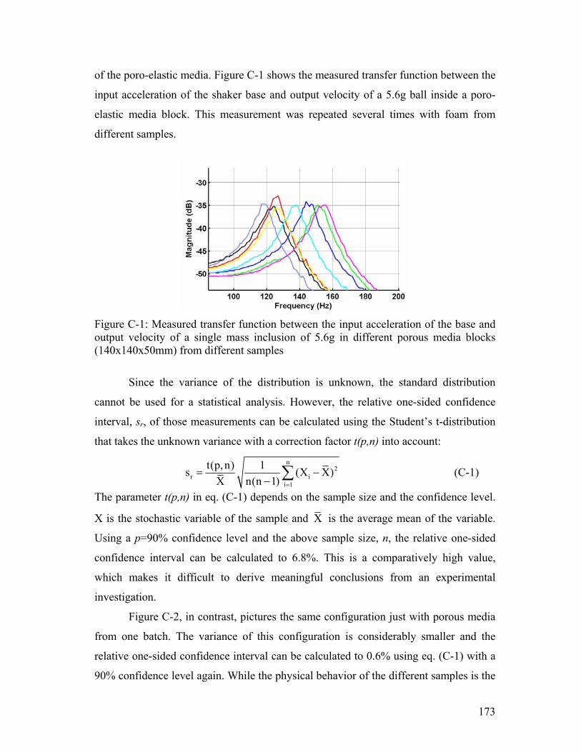
173

of the poro-elastic media. Figure C-1 shows the measured transfer function between the

input acceleration of the shaker base and output velocity of a 5.6g ball inside a poro-

elastic media block. This measurement was repeated several times with foam from

different samples.

Figure C-1: Measured transfer function between the input acceleration of the base and output velocity of a single mass inclusion of 5.6g in different porous media blocks (140x140x50mm) from different samples

Since the variance of the distribution is unknown, the standard distribution

cannot be used for a statistical analysis. However, the relative one-sided confidence

interval, sr, of those measurements can be calculated using the Student’s t-distribution

that takes the unknown variance with a correction factor t(p,n) into account:

n2

r ii 1

t(p, n) 1s (X X)X n(n 1) =

= −− ∑ (C-1)

The parameter t(p,n) in eq. (C-1) depends on the sample size and the confidence level.

X is the stochastic variable of the sample and X is the average mean of the variable.

Using a p=90% confidence level and the above sample size, n, the relative one-sided

confidence interval can be calculated to 6.8%. This is a comparatively high value,

which makes it difficult to derive meaningful conclusions from an experimental

investigation.

Figure C-2, in contrast, pictures the same configuration just with porous media

from one batch. The variance of this configuration is considerably smaller and the

relative one-sided confidence interval can be calculated to 0.6% using eq. (C-1) with a

90% confidence level again. While the physical behavior of the different samples is the

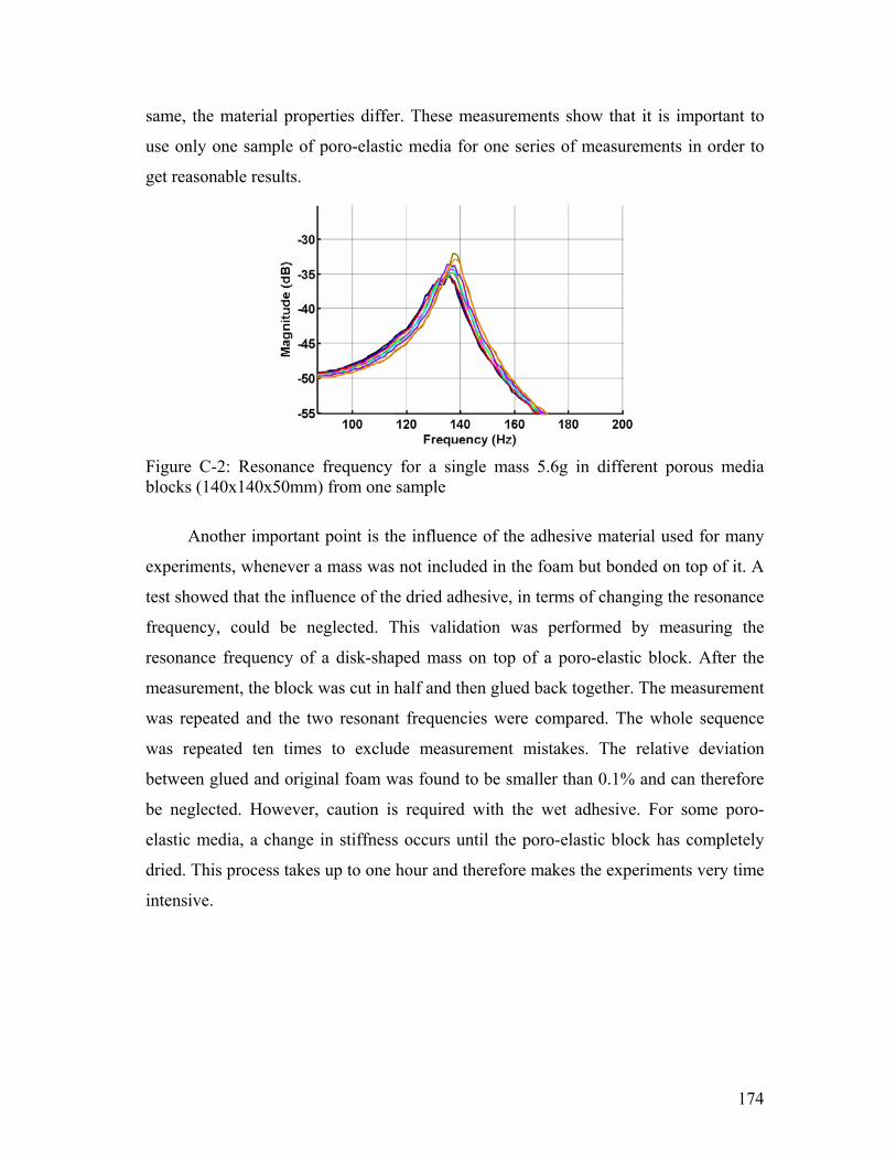
174

same, the material properties differ. These measurements show that it is important to

use only one sample of poro-elastic media for one series of measurements in order to

get reasonable results.

Figure C-2: Resonance frequency for a single mass 5.6g in different porous media blocks (140x140x50mm) from one sample

Another important point is the influence of the adhesive material used for many

experiments, whenever a mass was not included in the foam but bonded on top of it. A

test showed that the influence of the dried adhesive, in terms of changing the resonance

frequency, could be neglected. This validation was performed by measuring the

resonance frequency of a disk-shaped mass on top of a poro-elastic block. After the

measurement, the block was cut in half and then glued back together. The measurement

was repeated and the two resonant frequencies were compared. The whole sequence

was repeated ten times to exclude measurement mistakes. The relative deviation

between glued and original foam was found to be smaller than 0.1% and can therefore

be neglected. However, caution is required with the wet adhesive. For some poro-

elastic media, a change in stiffness occurs until the poro-elastic block has completely

dried. This process takes up to one hour and therefore makes the experiments very time

intensive.

175

BIBLIOGRAPHY [1] V. Mellert, I. Baumann, N. Freese, R. Weber, Impact of sound and vibration on

health, travel comfort and performance of flight attendants and pilots,

Aerospace Science and Technology (2007), doi:10.1016/j.ast.2007.10.009.

[2] M.A. Bellmann, H. Remmers, A. Röder, Environmental conditions for cockpit

and cabin crew members during long-haul flights. From experimental results to

a representative vibro-acoustic input vector for ANN and statistical approaches,

In 33rd German Annual Conference on Acoustics in Stuttgart, DAGA, 2007.

[3] J.F. Wilby, Aircraft interior noise, Journal of Sound and Vibration 190 (1996)

545-564.

[4] M. Carley, Propeller noise fields, Journal of Sound and Vibration, 233(2):255-

277, 2000.

[5] D.E. Bishop, Cruise flight noise levels in a turbojet transport airplane, Noise

Control 7, 37-42 (1961).

[6] N.J. Fleming, The silencing of aircraft, Journal of the Royal Aeronautical

Society, 50, pp. 639-676, 1946.

[7] R.E. Hayden, B.S. Murray, and M.A. Theobald, Boundary-layer-induced noise

in the interior of aircraft, NASA CR-172152, 1983.

[8] J.F. Wilby and E.G. Wilby, Measurements of propeller noise in a light

turboprop airplane, Journal of Aircraft 26, 40-47 (1989).

[9] W.V. Bhat, Use of correlation technique for estimating in-flight noise radiated

by wing-mounted jet engines on a fuselage, Journal of Sound and Vibration 17,

349-355 (1971).

[10] J.F. Wilby and F.L. Gloyna, Vibration measurements of an airplane fuselage

structure, II: jet noise excitation, Journal of Sound and Vibration 23, 467-486

(1972).

[11] E.J. Richards, Foreword, Journal of Sound and Vibration 17, 290-294.

[12] J.P. Carneal, Active structural acoustic control of double panel systems

including hierarchical control approaches, PhD Thesis, Virginia Polytechnic

Institute and State University, 1996.

176

[13] P.A. Nelson and S.J. Elliott, Active control of sound. Academic Press London,

1993.

[14] C.R. Fuller, Active control of sound transmission/radiation from elastic plates

by vibration inputs. I-Analysis, Journal of Sound and Vibration, 136 (1990) 1-

15.

[15] H.H. Bruderlin, Developments in aircraft sound control, Journal of the

Acoustical Society of America, 8, pp. 181-184, 1937.

[16] J.P. Carneal, Active structural acoustic control of double panel systems

including hierarchical control approaches, PhD Thesis, Virginia Polytechnic

Institute and State University, 1996.

[17] P. Gardonio, S.J. Elliott, Active control of structure-borne and airborne sound

transmission through double panel. Journal of Aircraft 36 (1999) 1023-1032.

[18] R.P.Goss, Acoustic program for the Grumman Gulfstream, AIAA Paper (1971)

71-783.

[19] G. SenGupta, Reduction of low frequency cabin noise during cruise condition

by stringer and frame damping, American Institute of Aeronautics and

Astronautics Journal 17 (1979) 229-236.

[20] C.I. Holmer, Approach to interior noise control, part I: damped trim panels,

Journal of Aircraft 22 (1985) 618-623.

[21] K.E. Heitman, J.S. Mixson, Laboratory study of cabin acoustic treatments

installed in an aircraft fuselage, Journal of Aircraft 23 (1986) 32–38.

[22] J.S. Mixson, L.A. Roussos, C.K. Barton, R. Vaicaitis, M. Slazak, Laboratory

tudy of add-on treatments for interior noise control in light aircraft, Journal of

Aircraft 20 (1983) 516-522.

[23] H. Baumgartl, Lightweight, Versatile All-rounder, Kunststoffe international

5/2006

[24] S.J. Estève and M.E. Johnson, Reduction of sound transmission into a circular

cylindrical shell using distribute vibration absorbers and helmholtz resonators,

Journal of the Acoustical Society of America 112 (2002) 2840–2848.

[25] C.I. Holmer, Approach to interior noise control, part II: self-supporting damped

interior shell, Journal of Aircraft 22 (1985) 729-733.

177

[26] H. Osman, M.E. Johnson, C.R. Fuller, P. Marcotte, Interior noise reduction of

composite cylinders using distributed vibration absorbers, 7th AIAA/CEAS

Aeroacoustics Conference (2001).

[27] M. Brennan, Vibration control using a tunable vibration neutraliser, in Proc

Instn Mech Engrs, vol. 211 part C, pp. 91–108, 1997.

[28] S. M. Lee, Normal vibration frequencies of a rectangular two-dimensional array

of identical point masses, Journal of Sound and Vibration, vol. 45(4), pp. 595–

600, 1975.

[29] D.M. Photiadis, Acoustics of a fluid loaded plate with attached oscillators. part

1. feynman rules, Journal of the Acoustical Society of America, vol. 102(1), pp.

348–357, 1997.

[30] C.R. Fuller, M.R.F. Kidner, X. Li, and C.H. Hansen, Active-Passive

Heterogeneous Blankets for Control of Vibration and Sound Radiation, In.

Proc. Active 04,Williamsburg, VA, USA,, Sep. 20–24 2004.

[31] M.R.F. Kidner, C.R. Fuller, B. Gardner, Increase in transmission loss of single

panels by addition of mass inclusions to a poro-ealstic layer: Experimental

investigation, Journal of Sound and Vibration, 294 (2006) 466–472.

[32] M.R.F. Kidner, K. Idrisi, J.P. Carneal and M.E. Johnson, Comparison of

Experiment, Finite Element and Wave Based Models for Mass Inclusions in

Poro-Elastic Layers, 14th International Congress on Sound and Vibration

(ICSV14), Cairns, Queensland, Australia, July 9-12, Paper 577 (2007).

[33] F. Sgard, N. Atalla., C.K. Amedin. “Vibro-acoustic behavior of a cavity backed

by a plate coated with a meso-heterogeneous porous material" Acta Acustica

United with Acustica, 93 (2007) 106-114.

[34] N. Atalla, C.K. Amedin, F. Sgard “Numerical and experimental investigation of

the vibro-acoustics of a plate backed cavity coated with a heterogeneous porous

material”, SAE meeting, Traverse City, USA, 2003, 2003-01-1453.

[35] K. Idrisi, M.E .Johnson, J.P. Carneal and M.R.F. Kidner, Passive control of

sound transmission through a double panel system using heterogeneous (HG)

blankets, Part II: HG parametric studies, Noise Con ’07 (2007).

178

[36] W.T. Thomson, Vibration Theory and Applications, Prentice-Hall,

IncEnglewood Cliffs, N.J., 1965.

[37] J.P. Den Hartog, Mechanical Vibrations, Dover Publications, McGraw Hill,

NY, 1934.

[38] F.A. Firestone, A new analogy between mechanical and electrical systems.

Journal of the Acoustical Society of America, 4 (1933) 249-267.

[39] F.A. Firestone, Twixt earth and sky with road and tube; mobility and classical

impedance analogies, Journal of the Acoustical Society of America, 4, 28(6),

1117-1153 (1956).

[40] G.J. O’Hara, Mechanical, Impedance and Mobility Concepts, U.S. Naval

Research Laboratory, Washington, D.C (1966).

[41] P. Gardonio, M.J. Brennan, On the origin and development of mobility and

impedance methods in structural dynamics, Journal of Sound and Vibration,

249 (2002) 557-573.

[42] R. Panneton, N. Atalla, An efficient finite element scheme for solving the three-

dimensional poroelastic problem in acoustics, Journal of the Acoustical Society

of America, 101 (1997) 3287 – 3298.

[43] Idrisi K., Johnson M. E., Carneal J. P., Toso A., Addition of mass inclusions to

a poro-elastic layer for improved passive control of aircraft interior noise: A

comparison between theory and experiment, Accepted for publication in Journal

of Sound and Vibration

[44] Idrisi K., Johnson M. E., Carneal J. P., Control of aircraft interior noise using

heterogeneous (HG) blankets, Proceedings of Meetings on Acoustics, Vol.1,

065001 (2008)

[45] Idrisi K., Johnson M. E., Carneal J. P., Passive control of sound transmission

through a double panel using heterogeneous (HG) blankets, Part I: Modeling

and validation, In. Proc. Noise-Con 2007 Reno Nevada, Oct. 22–24 2007

[46] Idrisi K., Johnson M. E., Multi-Bay double panel system with heterogeneous

blanket treatment: a comparison between theory and experiment, In 155th

Meeting Of The Acoustical Society Of America, 5th Forum Acusticum, And 9th

Congrès Français d’Acoustique, Paris, France, 29 June-4 July 2008

179

[47] Idrisi K., Johnson M. E., Carneal J. P., Passive control of sound transmission

through a double panel using heterogeneous (HG) blankets, Part III: HG

design strategies, In. Proc. Noise-Con 2007 Reno Nevada, Oct. 22–24 2007

[48] Idrisi K., Johnson M. E., Carneal J. P., Heterogeneous (HG) blanket design

strategies for passive control of aircraft interior noise, Accepted for publication

in Noise Control Engineering Journal

[49] Idrisi K., Johnson M. E, Toso A., Comparison of optimization routines for the

design of heterogeneous blankets, In. Proc. Noise-Con 2008, Dearborn, MI, 29-

30 July 2008

[50] Idrisi K., Bartylla D., Johnson M. E., Wagner A., Sensitivity of heterogeneous

blanket design to parameter variation, In. Proc. Noise-Con 2008, Dearborn, MI,

29-30 July 2008

[51] Idrisi K., Johnson M. E., Carneal J. P., Theurich D., A study on the behavior of

mass inclusions added to a poro-elastic layer, manuscript submitted in October

2008 to Journal of Sound and Vibration

[52] M.A. Biot, Theory of propagation of elastic waves in a fluid-saturated porous

solid. I. Low-frequency range. The Journal of the Acoustical Society of

America, 28 (1956) 168 – 178.

[53] J.F. Allard, Propagation of sound in porous media, modeling sound absorbing

materials, Elsevier Science Publishers LTD., London, 1993.

[54] Idrisi K., Wagner A., Johnson M. E., Bartylla D., On heterogeneous blankets:

Analytical solution for the interaction between masses and poro-elastic layers,

In 155th Meeting Of The Acoustical Society Of America, 5th Forum Acusticum,

And 9th Congrès Français d’Acoustique, Paris, France, 29 June-4 July 2008

[55] P. Gardonio, M.J. Brennan, Active isolation of structural vibration on a

multiple- degree-of-freedom system, Part I: The dynamics of the system.

Journal of Sound and Vibration 207 (1997) 61-93.

[56] G. Warburton, The vibration of rectangular plates. Proceedings of the

Institution of Mechanical Engineers, 168 (1954) 371-384.

180

[57] R. Panneton, N. Atalla, An efficient finite element scheme for solving the three-

dimensional poroelastic problem in acoustics. Journal of the Acoustical Society

of America, 101 (1997) 3287 – 3298.

[58] L. Kinsler, A. Frey, A. Coppens, J. Sanders, Fundamentals of acoustics, Wiley,

New York, 1999.

[59] P.A. Nelson and S.J. Elliott: Active control of sound. Academic Press, London,

1993

[60] S.J. Elliott and M.E. Johnson, Radiation modes and the active control of sound

power. Journal of the Acoustical Society of America, 94 (1993) 2194–2204.

[61] M.R. Bai, M. Tsao, Estimation of sound power of baffled planar sources using

radiation matrices. Journal of the Acoustical Society of America, 112 (2002)

876-883.

[62] A.P. Berkhoff, Sensor scheme design for active structural acoustic control.

Journal of the Acoustical Society of America, 108 (2000) 1037-1045.

[63] P. Gardonio, M.J. Brennan, On the origin and development of mobility and

impedance methods in structural dynamics. Journal of Sound and Vibration,

249 (2002) 557-573.

[64] P. Gardonio, M.J. Brennan, Mobility and impedance methods in structural

dynamics, Spon Press, New York, 2004.

[65] P. Gardonio, and M.J. Brennan, Mobility and impedance methods in structural

dynamics: an historical review, ISVR Technical Report 289, Southampton,

University of Southampton, 2000.

[66] K.A. Mulholland, H.D. Parbrook, A. Cummings, The transmission loss of a

double panel. Journal of Sound and Vibration, 6 (1967) 324-334.

[67] A. Gautam, C.R. Fuller, J.P. Carneal, Application of the Heterogeneous

blankets (HG blankemts) for controlling the base structure vibration

levels, Noise Con ’05 (2005).

[68] C.R. Fuller, S.J. Elliott and P.A. Nelson. Active Control of Vibration (1st

Edition ed.), Academic Press, London (1996).

[69] B.T. Wang, C.R. Fuller and E.K. Dimitriadis, “Active control of noise

transmission through rectangular plates using multiple piezoelectric or point

181

force actuators. Journal of the Acoustical Society of America, 90 (1991) 2820 –

2830.

[70] M.E. Johnson, Active Control of Sound Transmission, PhD Thesis, University

of Southampton, 1996.

[71] K.R. Matthews, Elementary linear Algebra, Dept. of Mathematics, University

of Queensland (1991), http://www.numbertheory.org/book/ (Accessed 21

February 6, 2008).

[72] Idrisi K., Johnson M. E., Carneal J. P., Kidner M. R. F., Passive control of

sound transmission through a double panel using heterogeneous (HG) blankets,

In. 153rd Meeting of Acoustical Society of America (2007) in Salt Lake City,

Journal of the Acoustical Society of America, Vol. 121, No. 5, Pt. 2, May 2007.

[73] A.W. Leissa, Vibration of Plates, NASA SP-160, 1969.

[74] F.A. Firestone, “The mobility method of computing the vibration of linear

mechanical and acoustical systems: mechanical-electrical analogies, Journal of

Applied Physics, 9, 373-387 (1938).

[75] C.R. Fuller, M.R.F. Kidner, X. Li, and C.H. Hansen, Active-Passive

Heterogeneous Blankets for Control of Vibration and Sound Radiation, In.

Proc. Active 04,Williamsburg, VA, USA,, Sep. 20–24 2004.

[76] N. Alujević, K.D. Frampton, P. Gardonio, Stability and performance of a smart

double panel with decentralized active dampers, The American Institute of

Aeronautics and Astronautics Journal. 46(7), 2008, 1747-1756.

[77] M.E. Johnson, J.P. Carneal, C. R. Fuller and H. Osman, Control of shock

transmission through an aerospace structure using optimally damped distributed

vibration absorbers, 12th International Congress on Sound and Vibration Jul.

11-14th 2005.

[78] H. Frahm, Device for damping vibrations of bodies, U.S. Patent No. 989958,

1909.

[79] J. Dayou, M.J. Brennan, Global control of structural vibration using multiple-

tuned tunable vibration neutralizers, Journal of Sound and Vibration (2002)

258(2), 345–357.

182

[80] R.G. Jaquot, Suppression of random vibration in plates using vibration

absorbers, Journal of Sound and Vibration (2001) 248(4), 585-596.

[81] P. Hagedorn, Lineare Schwingungen kontinuierlicher mechanischer Systeme,

Springer-Verlag, Berlin, Heidelberg, New York, 1989.

[82] N.H. Schiller, Decentralized control of sound radiation from periodically

stiffened panels, PhD Thesis, Virginia Polytechnic Institute and State

University, 2007.

[83] K.U. Ingard and T.A. Dear, Measurements of acoustic flow resistance. Journal

of Sound and Vibration 103 (1985) 567–572.

[84] J. Park, Measurements of the frame acoustic properties of porous and granular

materials. Journal of the Acoustical Society of America, 118 (2005) 3483 –

3490.

[85] A. P. S. Selvadurai: Mechanics of poroelastic media , Kluwer Academic

Publishers, Dordrecht, 1996

[86] R. de Boer: Theory of porous media: Highlights in historical development and

current state, Springer, Berlin, Heidelberg and New York, 2000

[87] K. Attenborough: Acoustical characteristics of porous materials, Physics

Reports 82(3), 1982, 179 – 227

[88] W. Becker and D. Gross: Mechanik elastischer Körper und Strukturen.

Springer, Berlin and Heidelberg, 2002