hess-2018-165 Title of the manuscript: Multimodel assessment of ...

Reply to Reviewer 1 comments

Manuscript number: hess-2018-165 Title of the manuscript: Multimodel assessment of climate change-induced hydrologic impacts for a Mediterranean catchment. Authors: E. Perra, M. Piras, R. Deidda, C. Paniconi, G. Mascaro, E.R. Vivoni, P. Cau, P.A. Marras, R. Ludwig, S. Meyer.

We thank Reviewer 1 for her/his comments on our manuscript. In the following, the specific comments by Reviewer 1 are copied in bold font, followed by our replies to each point.

1) On page 6, lines 187-193 the authors introduce the climate models used in their analysis and later they specify the spatial and temporal resolution of the models (25 km, 24 h) and of the downscaled variables (5 km, 1 h). However, we do not know if the analyses presented on section 4.1 were carried out on the original model output at coarse resolution or on the downscaled variables. If the analyses were carried out directly on model output, model resolution (25 km) is similar to basin size, and the process of computing basin averages should be explained in better detail. If the analyses were carried out on the downscaled variables, I think a discussion of the possible influence of bias correction and downscaling on the results should be added.

The analyses presented on section 4.1 were carried out using the downscaled and bias-corrected variables of precipitation and temperature, since we need accurate estimations of the hydrologic variables to run the hydrologic models. This information is now better conveyed in the revised manuscript (lines 258-259). With reference to the last suggestion, we agree on the importance of studying the effect of bias correction and downscaling on the results. This issue was examined for the Rio Mannu catchment by Piras et al. (2014), cited in the paper, and we are currently conducting a separate study on the effect of different downscaling techniques on the hydrologic cycle of another Sardinian basin.

2) I think model calibration also deserves additional discussion. On page 4, lines 112- 114, the authors say: “The hydrologic models were independently calibrated and validated against observed data, with each modelling group using the type of data most suitable to that model, such as field-scale soil moisture, evapotranspiration patterns, and discharge”. I have the impression that some of the differences observed in model behaviour, like the discrepancies in the monthly distribution of soil water content shown in Figure 8, may be explained by how the different models were calibrated. Perhaps the authors should consider a brief discussion of this issue.

We have added at the end of Section 3.1 further details on the calibration and validation procedures for the five hydrological models (lines 193-209).

3) The authors provide a reference to Duveiller et al., 2016 to introduce their bias coefficient

“alpha”. I found it to be a very interesting paper and thank the authors for calling my attention to it. From reading this paper, I gathered the impression that it was intended for comparison of large data sets. However, the authors chose to apply it only to monthly averages, although they had the full time series available for comparison. Perhaps they should explain the reasons for their decision.

We agree with the reviewer that it would have been interesting to apply these performance indices to the time series at their original resolution. However we are using climate model outputs, and the results must be averaged to have projections of climate variability. For this reason we decided to apply the Pearson and Duveiller coefficients using the monthly averages.

4) Following on the same argument, I think Figure 3 would be more useful if it included examples of scatter plots corresponding the four cases shown. This would allow the reader to grasp the kind of agreement obtained in each of the four cases.

We have added the scatter plots in the revised Figure 3.

5) The shift in the seasonal distribution of actual evapotranspiration between SWAT and WASIM observed in Figure 9 and the rest of the models may also deserve additional discussion. Could it be due to limited water availability in the summer? May it be due to spring vegetation growth?

The SWAT and WASIM models anticipate the peak of actual evapotranspiration during spring months: this could be explained by the fact that these models incorporate also vegetation processes, and also by limited water availability in the summer. As we can see from Fig. 8c, SWAT and WASIM simulate very low soil water content during July and August. This point is now added in the revised manuscript (lines 350-352).

TECHNICAL CORRECTION From the formal standpoint, the paper is very well written, correctly organized and adequately illustrated with tables and figures. Interpretation of Figure 5 is handicapped by the fact that the upper row contains four cases for comparison and the lower row contains five cases. I would suggest resizing one of the two so that both rows plot on the same scale.

We have resized the lower panel to better interpret Figure 5.




1) Introduction: while describing the state of the art, it would be appropriate, in addition to listing different sources of uncertainty, also highlight with appropriate bibliographic references that the uncertainty is greater in the climatic modeling of future scenarios rather than in hydrological models.

We have added a couple of references (Hawkins and Sutton, 2009; Pechlivanidis et al., 2017) in the second paragraph of the Introduction that address this point.

2) L.187: According to the sentence “those [models] exhibiting the best performance” it may be useful to provide some further explanations about the criteria involving the choice of climate models.

When assessing a climate model’s skills, it is important to examine its ability to reproduce the annual averages and seasonal variability of precipitation and surface temperature. This is stated in the revised manuscript as follows (lines 211-215): “Deidda et al. (2013) analyzed the open-access outputs of fourteen GCM-RCM combinations from the ENSEMBLES project to identify those exhibiting the best performance in terms of representing the intra-annual variability of precipitation and temperature in the present climate for the seven study sites of the precursor European project. For each study site, the selected set of climate model data was validated using the E-OBS dataset, a high quality pan-European gridded observational dataset of daily precipitation and temperature (Haylock et al., 2008).”

3) L.191: Although I am aware of the large amount of work done both in the calibration and validation of hydrological models and for what concerns the determination of the climatic scenarios, it is worth highlighting that the SRES scenarios used in the paper are now outdated and that perhaps it would have been more useful to refer to the new RCP scenarios. It would be appropriate to motivate this choice.

This study is based on data and model implementations that were part of a European-funded research project that ran from 2010 to 2013 (Ludwig et al., 2010, cited on line 93; see also the Acknowledgements for further details on this project). The new RCP scenarios were not available at the

time of the project.

4) L.205: The authors use a bias coefficient “alpha” proposed by Duveiller et al. (2016), which is interesting from a statistical point of view, but in terms of graphic rendering it does not seem very readable, especially if the number of models is expected to increase. In this sense, Figures 5, 10 and 11 provide summary indications not allowing to appreciate differences, not necessarily macroscopic, between models. The use of tables could better integrate the information content of the aforesaid figures.

We have added, as supplementary material to the paper, four tables that provide the actual values of the Pearson and bias coefficients for the different analyses performed.

5) In the paper it would be useful a "Discussion" section dedicated to a detailed description of the causes of the main differences between the hydrological models, since they are only partially hinted at when results are introduced and at the end of Conclusions.

We have moved the discussion on the differences that emerge in the analysis of agreement from the last paragraph of the Conclusions to the last paragraph of Section 4.3 (Agreement analysis), and we have added an additional consideration to this discussion (lines 412-413).

6) It would also be useful to evaluate such differences among the models also in the light of their performances compared to the observed data, which is not evident in the manuscript.

See the next point.

7) To this end, at least it is necessary to recall in detail the results related to the performances of the single models, not only reporting citations (ll. 114-115), among which there is a manuscript in preparation.

We have added at the end of Section 3.1 more details on the single model performances against observed data during the calibration procedures (lines 193-209).

8) The Conclusions should be improved. For example, it is said (ll, 418-420) "CATHY, for instance, has the most detailed subsurface representation of the five models, and as such will tend to retain more water in subsurface storage, making some of this water available for subsequent evaporation". Is it possible to achieve a more general conclusion from this statement? Is it possible to state only that a more detailed model increases the subsurface storage or one can infer that a more detailed model is more credible and therefore the forecast of increased subsurface storage is to be considered more likely? The same is true for models with a more detailed description of vegetation. This question can be answered only considering also the performances with respect to the observations (see previous point).

This is a holy grail question that is difficult to answer. As the reviewer points out, assessing the actual

worth or correctness, even in likelihood terms, of the different models would require much more extensive comparison against observations. This was not the intent of our study, and indeed, as noted in the added section on the calibration procedures, two of the model parameterizations, CATHY’s and TOPKAPI’s, were in large part based directly on the tRIBS calibration results. Since we are dealing with hydrologic models that represent watershed processes at very different levels of detail, and since the best climate/hydrologic model coupling for our specific study site is not known a priori, our focus instead was on using a multimodel platform to provide a range of possible hydrologic responses for climate change scenarios, while at the same time quantifying in some way the level of interagreement between models based on these different responses.




1) Lines 187-190: Since the climate models ensemble adopted in the study is limited to four members, I believe that a deeper discussion of the criteria adopted in this selection could be beneficial.

When assessing a climate model’s skills, it is important to examine its ability to reproduce the annual averages and seasonal variability of precipitation and surface temperature. This is stated in the revised manuscript as follows (lines 211-215): “Deidda et al. (2013) analyzed the open-access outputs of fourteen GCM-RCM combinations from the ENSEMBLES project to identify those exhibiting the best performance in terms of representing the intra-annual variability of precipitation and temperature in the present climate for the seven study sites of the precursor European project. For each study site, the selected set of climate model data was validated using the E-OBS dataset, a high quality pan-European gridded observational dataset of daily precipitation and temperature (Haylock et al., 2008).”

2) I think that the paper could benefit from the inclusion of a sub-section (or Supplementary Material) in which the calibration methods, metrics, and observations adopted are shortly described for each hydrological model setup.

We have added at the end of Section 3.1 further details on the calibration and validation procedures for the five hydrological models (lines 193-209). 3) Since a robust calibration and validation of each hydrological model is required for ad- dressing the research questions here proposed, I feel that the manuscript could benefit of a more detailed discussion of the differences between simulated and observed streamflow time series.

See the additional paragraph on model calibration mentioned above.

4) Section 4.3. In line with the previous comment, I also think that the performances of the different models in reproducing soil water content and ET should be presented (even in a concise way or as Supplementary Material).

The only model that used soil water content was WASIM, while tRIBS and SWAT were calibrated against discharge observations. See again the new paragraph on model calibration.

5) Finally, I feel that the discussion section could be improved trying to understand if the discrepancies between the models are epistemic in their nature (i.e., related to the different representation of the various hydrological processes) or may be related to other factors, like e.g. calibration methods and type of observational data used for evaluating model performances.

In our study epistemic differences are important since the models are structurally quite different from each other, representing critical processes (subsurface flow, evapotranspiration, etc) in very different ways and to varying levels of complexity. The possible contribution of these structural factors in explaining the performance results obtained is highlighted in the paper. The comparative performance between models will also depend on the response variables or observation data being examined, in part because of the structural differences just mentioned, but also for other reasons not explored in our study. The important issue of the role of calibration methods is also not explored, given that the five models were independently calibrated and that the paper is mainly focused on assessing possible hydrologic response impacts to climate change based on a multimodel platform.

1

Multimodel assessment of climate change-induced hydrologic impacts for a Mediterranean catchment Enrica Perra1,2, Monica Piras1,3, Roberto Deidda1,3, Claudio Paniconi2, Giuseppe Mascaro3,4, Enrique R. Vivoni4, Pierluigi Cau5, Pier Andrea Marras5, Ralf Ludwig6, Swen Meyer6,7 1Dipartimento di Ingegneria Civile, Ambientale ed Architettura, Università degli Studi di Cagliari, Cagliari, Italy 5 2Centre Eau Terre Environnement, Institut National de la Recherche Scientifique, Quebec City, Canada 3Consorzio Interuniversitario nazionale per la Fisica dell’Atmosfere e dell’Idrosfere, Tolentino, Italy 4School of Sustainable Engineering and the Built Environment and School of Earth and Space Exploration, Arizona State University, Tempe, Arizona 5Centro di Ricerca, Sviluppo e Studi Superiori in Sardegna, Pula, Cagliari, Italy 10 6Physical Geography and Environmental Modeling, Department of Geography, Ludwig-Maximilians-Universitaet Muenchen, Munich, Germany 7Leibniz-Institut für Gemüse- und Zierpflanzenbau Großbeeren/Erfurt e.V., Grossbeeren, Germany

Correspondence to: Enrica Perra ([email protected])

Abstract. This work addresses the impact of climate change on the hydrology of a catchment in the Mediterranean, a region 15

that is highly susceptible to variations in rainfall and other components of the water budget. The assessment is based on a

comparison of responses obtained from five hydrologic models implemented for the Rio Mannu catchment in southern

Sardinia (Italy). The examined models – CATchment HYdrology (CATHY), Soil and Water Assessment Tool (SWAT),

TOPographic Kinematic APproximation and Integration (TOPKAPI), TIN-based Real time Integrated Basin Simulator

(tRIBS), and WAter balance SImulation Model (WASIM) – are all distributed hydrologic models but differ greatly in their 20

representation of terrain features and physical processes and in their numerical complexity. After calibration and validation,

the models were forced with bias-corrected, downscaled outputs of four combinations of global and regional climate models

in a reference (1971-2000) and a future (2041-2070) period under a single emission scenario. Climate forcing variations and

the structure of the hydrologic models influence the different components of the catchment response. Three water

availability response variables – discharge, soil water content, and actual evapotranspiration – are analyzed. Simulation 25

results from all five hydrologic models show for the future period decreasing mean annual streamflow and soil water content

at 1 m depth. Actual evapotranspiration in the future will diminish according to four of the five models due to drier soil

conditions. Despite their significant differences, the five hydrologic models responded similarly to the reduced precipitation

and increased temperatures predicted by the climate models, and lend strong support to a future scenario of increased water

shortages for this region of the Mediterranean basin. The multimodel framework adopted for this study allows estimation of 30

the agreement between the five hydrologic models and between the four climate models. Pairwise comparison of the climate

and hydrologic models is shown for the reference and future periods using a recently proposed metric that scales the Pearson

correlation coefficient with a factor that accounts for systematic differences between datasets. The results from this analysis

2

reflect the key structural differences between the hydrologic models, such as a representation of both vertical and lateral

subsurface flow (CATHY, TOPKAPI, and tRIBS) and a detailed treatment of vegetation processes (SWAT and WASIM). 35

1 Introduction

Climate studies agree on the prediction that the Mediterranean area will be particularly affected by changes under global

warming (IPCC, 2014). This region, in fact, has been singled out as one of the hotspots in future climate change predictions

(Giorgi, 2006), due to higher susceptibility to more frequent and more intense extreme events. In addition, observations

during the last decades indicate that mean and extreme temperatures have increased in several Mediterranean regions 40

(Xoplaki et al., 2003; Del Río et al., 2011; El Kenawy et al., 2011; Acero et al., 2014) and that precipitation has diminished,

especially in the warm season (Giorgi and Lionello, 2008; Sousa et al., 2011; Vicente-Serrano and Cuadrat-Prats, 2007).

Climate change impact assessment at the catchment scale is usually conducted through a procedure that involves the

following steps (e.g., Xu et al., 2005): (i) selection of global climate models (GCMs) and regional climate models (RCMs) 45

for future climate predictions; (ii) correction of the discrepancies between simulated and observed climatological features;

(iii) application of downscaling techniques to increase the coarse scale of climate model outputs to the finer resolutions

required by hydrologic models; and (iv) use of downscaled outputs as forcing for the calibrated hydrologic models to

simulate the basin hydrologic response (Sulis et al., 2011, 2012; Piras et al., 2014; Hawkins et al., 2015; Majone et al., 2016;

Meyer et al., 2016). Each of these steps is affected by uncertainties (Xu and Singh, 2004), including the choice of emission 50

scenarios and climate forcings (Giorgi and Mearns, 2002; Tebaldi et al., 2005; Pechlivanidis et al., 2017), the selection of

downscaling techniques (Wood et al., 2004; Im et al., 2010) and hydrologic model (Clark et al., 2008; Jiang et al., 2007;

Dams et al., 2015), and the availability of observed data required for calibration and validation of both downscaling

techniques and hydrologic models. Hawkins and Sutton (2009) estimate that by the end of the century, the emission

scenarios will represent the dominant source of uncertainty in climate projections. 55

One approach to dealing with uncertainties is to use multiple climate and hydrologic models (Bosshard et al., 2013;

Cornelissen et al., 2013; Gädeke et al., 2014; Najafi et al., 2011). For example, Bae et al. (2011) compared in a Korean basin

three semi-distributed hydrologic models forced with outputs from thirteen GCMs and three greenhouse gas emission

scenarios. Their results show that the hydrologic models can produce major differences in runoff change considering the 60

same climate change scenarios, in particular during the dry season. Bastola et al. (2011) examined the role of hydrologic

model uncertainties (parameter and structural uncertainty) using four conceptual hydrologic models and six climate change

scenarios within the generalised likelihood uncertainty estimation (GLUE) and Bayesian model averaging (BMA) methods.

The results for the four Irish catchments considered showed a tendency of increasing flow in winter and decreasing flow in

summer. Thompson et al. (2013) demonstrated for the Mekong river in southeast Asia that GCM-related uncertainty in 65

3

climate change projections is generally larger than that related to the use of three hydrologic models, which simulate the

same direction of change in mean discharge. However, hydrologic model related-uncertainty is not negligible and in some

cases is of a similar magnitude to GCM-related uncertainty. Vansteenkiste et al. (2014) used an ensemble of hydrologic

models, from lumped conceptual to distributed physically based, to assess the impact of climate change on the Grote Nete

basin (Belgium). The uncertainty in the hydrologic impact results was evaluated by the relative change in runoff volumes 70

and peak and low flow extremes from historical and future climate conditions. Large differences in model predictions were

found, especially under low flow conditions Using an ANOVA approach, Bosshard et al. (2013) assessed the uncertainties

induced by climate models, bias correction methods, and hydrological models using the output of eight RCMs for the Upper

Rhine. The results indicate that some of the uncertainties are not attributable to individual modeling chain components but

rather they depend on the interactions between these components, and that overall the greatest contribution to uncertainty 75

derives from the climate models. Maurer et al. (2010) investigated the effect of hydrologic model structure by comparing a

lumped and a distributed model driven by twenty-two climate model outputs for three California watersheds. The projected

percent changes in monthly discharge did not significantly differ between the two models, except for extreme flows and

during summer months.

80

In this study, we characterize the agreement between both climate and hydrologic predictions in the Rio Mannu catchment, a

small Mediterranean basin located in a semiarid region in Sardinia (Italy). For this aim, we use an ensemble of climate and

hydrologic models, including four combinations of GCMs and RCMs and a set of five hydrologic models of varying

structural complexity, from conceptual to physically-based. This is the first study wherein a wide range of distributed

hydrologic models forced with outputs of different climate models is applied to a Mediterranean catchment to assess the 85

impact of climate change. Moreover, unlike many previous studies, we focus on a set of variables characterizing and

affecting the water balance at the catchment scale, including precipitation, air temperature, discharge, soil water content in

the first meter, and actual evapotranspiration. The results are discussed in the context of the process representations for each

model and within a rigorous analysis of agreement framework. For the latter a new metric, proposed by Duveiller et al.

(2016), will be used to compare model results for reference and future periods using correlation and bias coefficients. 90

2 Study area

The study site is the Rio Mannu di San Sperate at Monastir basin, located in southern Sardinia, Italy (Fig. 1). The Rio Mannu

basin was one of the seven study sites of a European-funded climate change research project (Ludwig et al., 2010). Amongst

the reasons for selecting the Rio Mannu site for this project is the presence of an agricultural research station within its

boundaries, where extensive field characterization studies could be undertaken, and the vulnerability of this region to 95

climatic extremes (e.g., several prolonged drought periods over the past decades). Over the course of the European project,

4

several field and modeling activities of relevance to this study were undertaken (Cassiani et al., 2012; Marras et al., 2014;

Filion et al., 2016; Meyer et al., 2016).

The Rio Mannu catchment drains an area of 473 km2 and is characterized by a gently rolling topography, with an elevation 100

range from 66 to 962 m a.s.l. and a mean slope of 17 %. The mean annual precipitation is 600 mm and the mean temperature

ranges from 9 °C in January to 25 °C in July-August. The climate is typically Mediterranean, with about 90 % of the annual

rainfall falling from October to April. The discharge regime is characterized by low flows (less than 1 m3/s) for most of the

year (Mascaro et al., 2013a). Precipitation, temperature, and discharge within and around the Rio Mannu catchment have

been collected at a daily time scale, albeit intermittently and not always coincidentally, since 1925. As shown in Fig 2, soil 105

texture in the Rio Mannu catchment is dominated by three classes, including clay loam–clay (37 %), sandy loam–loam (32

%), and sandy loam–sandy clay loam (20 %). Agriculture (∼ 48 %) and sparse vegetation (∼ 26 %) are the dominant land use

classes. A more detailed description of the basin land surface properties can be found in Mascaro et al. (2013b).

3 Methods

An impact assessment framework was developed during the precursor European project wherein the best performing four 110

GCM-RCM combinations from the ENSEMBLES project (van der Linden and Mitchell, 2009) were selected for each study

site. The daily GCM-RCM outputs at 25 km resolution for a reference (1971-2000) and a future (2041-2070) period were

bias corrected and statistically downscaled. For the Rio Mannu site, the downscaled data were then used to force five

hydrologic models for the reference and future periods. The hydrologic models were independently calibrated and validated

against observed data, with each modeling group using the type of data most suitable to that model, such as field-scale soil 115

moisture, evapotranspiration patterns, and discharge. More details on the model calibration are given after the model

descriptions below.

3.1 Hydrologic models

The five hydrologic models examined in this study are: CATchment HYdrology (CATHY), Soil and Water Assessment Tool

(SWAT), TOPographic Kinematic APproximation and Integration (TOPKAPI), TIN-based Real time Integrated Basin 120

Simulator (tRIBS), and WAter balance SImulation Model (WASIM). The models differ greatly in their representation of

terrain features and physical processes and in their numerical complexity, but they are all able to account for the spatial

variability of meteorological inputs and land surface properties, albeit at different levels of detail. Table 1 summarizes the

characteristics of each hydrologic model, highlighting the main differences between them. For more detail, the reader is

referred to the references provided below in the description of each model. 125

Enrica Perra � 30/5/18 11:27Deleted: (Cau et al., 2005; Mascaro et al., 2013b; Meyer et al., 2016; Perra et al., manuscript in preparation).

5

CATHY is a physically based numerical model that resolves in a detailed manner the interaction between subsurface and 130

surface water (Camporese et al., 2010). The surface module is based on the resolution of a one-dimensional diffusion wave

approximation of the Saint Venant equation for overland and channel routing (Orlandini and Rosso, 1996). The subsurface

module solves the three-dimensional Richards equation that describes flow in variably saturated porous media (Paniconi and

Wood, 1993). The surface grid, catchment boundaries, and rill and channel flow paths are delineated via topographic

analysis of digital elevation maps. Model inputs consist of spatially variable or homogeneous meteorological data and 135

surface properties for each zone and layer of the basin. CATHY outputs include time series of actual fluxes and discharge

and at any location in the stream network and spatial maps of several hydrological variables (e.g., pressure, saturation,

ponding) at specified times. The CATHY model has been used in many exploratory studies, benchmarking exercises, and

real catchment applications, including the assessment of climate change impacts (e.g., Gauthier et al., 2009; Sulis et al.,

2011; Gatel et al., 2016; Kollet et al., 2017; Scudeler et al., 2017). 140

SWAT is a conceptual, semi-distributed model that allows the evaluation of climate and land use impacts on water resources,

sediments, and agriculture through a physical representation of hydrologic processes, soil temperature, plant growth,

nutrients, pesticides, and land use (Arnold et al., 1998). In SWAT, a watershed is divided into multiple subwatersheds, which

are then further divided into hydrologic response units (HRUs) that consist of homogeneous land use, management, 145

topographic, and soil characteristics. The HRUs are represented as a percentage of the subwatershed area and need not be

contiguous or spatially identified. A daily time step is adopted in the simulation of hydrologic processes. Surface runoff is

estimated using the Soil Conservation Service (SCS) curve number procedure, and the movement of soil moisture vertically

within the soil profile is simulated using a one-dimensional tipping bucket approach. Model inputs consist of meteorological

data and surface and vegetation properties. SWAT outputs include time series of discharge at any location in the stream 150

network and actual evapotranspiration and soil water content integrated over the basin. Its applications range from

engineering/practical aims to research studies (e.g., Arnold et al., 1999; Cau et al., 2005; Mausbach and Dedrick, 2004; Volk

et al., 2007).

TOPKAPI is a physically based distributed rainfall-runoff model that combines basin topography with the kinematic 155

approach (Ciarapica and Todini, 2002). The model consists of five modules that simulate the main hydrologic processes

including subsurface flow, overland flow, channel flow, evapotranspiration, and snowmelt. These can be simulated at an

hourly time step. Four nonlinear reservoir differential equations solved using a two-dimensional finite difference method are

used to describe subsurface, overland, and channel flow. The model uses a regular grid to represent the terrain and is

computationally efficient and thus suitable to be applied for real-time flood forecasting. Model inputs consist of 160

meteorological data and spatial maps of surface properties (e.g., soil texture and land cover maps). TOPKAPI outputs

include time series of discharge at any location in the stream network and actual evapotranspiration and soil water content

integrated over the basin. TOPKAPI has been successfully implemented as a research and operational hydrologic model in

6

several catchments worldwide (e.g., Liu and Todini, 2002; Bartholomes and Todini, 2005; Liu et al., 2005; Martina et al.,

2006). 165

tRIBS is a physically based spatially distributed model that reproduces a range of hydrologic processes (Ivanov et al. 2004)

including canopy interception and transpiration, evaporation from bare and vegetated soils, infiltration and soil moisture

redistribution, shallow subsurface transport, and overland and channel flows (Mascaro et al., 2013b). Terrain features are

represented via triangulated irregular networks (TINs). In each Voronoi polygon derived from TINs the coupled energy and 170

water balances are computed, while the infiltration scheme is based on the resolution of the two-dimensional modified

Green-Ampt model. A kinematic wave routing model is used to simulate transport of water in the channel network. Model

inputs include spatial maps of surface properties (e.g., soil texture and land cover maps). tRIBS outputs include time series

of discharge at any location in the stream network and spatial maps of several hydrological variables (e.g., actual

evapotranspiration, soil water content at different depths) at specified times or integrated over the simulation period (Piras, 175

2014). The model has been applied across a large range of scales in the areas of hydrometeorology, climate change, and

ecohydrology (e.g., Liuzzo et al., 2010; Mascaro et al., 2010, 2015; Mahmood and Vivoni, 2014). Recently, Piras (2014) and

Piras et al. (2014) applied tRIBS in the Rio Mannu catchment to evaluate the hydrologic impact of climate change.

WASIM is a physically based and fully distributed hydrologic model (Schulla, 2015) originally developed to evaluate the 180

influence of climate change on water balance and runoff regime in pre-alpine and alpine river catchments (Schulla, 1997).

WASIM runs in a grid-based structure and represents vertical fluxes in the unsaturated zone by the one-dimensional

Richards equation, which is solved with a finite difference scheme. Discharge routing is performed by a kinematic wave

approach. After the translation of the wave for all channels, a single linear storage is applied to the routed discharge

considering the effect of diffusion and retention (Schulla and Jasper, 2001). Sub-modules are available for various 185

hydrologic variables such as interception, discharge, runoff, snowmelt, and evapotranspiration. Model inputs consist of

meteorological data and spatial maps of surface properties (e.g., soil texture and land cover maps). WASIM outputs include

time series of discharge at any location in the stream network and spatial maps of several hydrological variables (e.g., actual

evapotranspiration, soil water content) at specified times or integrated over the simulation period. WASIM has been

previously applied for hydrologic issues such as impact analysis for river basins and hydrologic forecasting (e.g., 190

Cornelissen et al., 2013; Jasper et al., 2002; Kunstmann et al., 2006; Meyer et al., 2016).

The calibration procedures varied from one model to the next, owing to the significant structural differences between the

models, and to the fact that each modeling group worked independently of the others, within different project frameworks

and timelines. tRIBS was calibrated manually against discharge observations at the outlet for the year 1930, and validated for 195

the 1931-1932 period (Mascaro et al., 2013b). The calibration focused on its two most sensitive parameters, saturated

hydraulic conductivity at the surface and the decay parameter that models the variation of conductivity with soil depth.

7

Model performance was assessed based on a comparison between observed and simulated discharge and flood duration

curves, quantified using the Nash-Sutcliffe index. For WASIM, Meyer et al. (2016) conducted a soil sampling campaign on

the Rio Mannu catchment in 2010-2011. They tested the performance of different regionalization methods for soil texture 200

against soil moisture field measurements, and derived a new soil texture map based on the best of these methods. WASIM

was then run with two different soil configurations – the new map and the available regional soil map – and the sensitivity to

model outputs was examined. The model was validated with spatially distributed evapotranspiration rates using the triangle

method (Jiang and Islam, 1999), and performances were quantified using the coefficient of determination. The SWAT model

parameterization was based on a regional scale calibration of the model’s soil parameters against discharge observations 205

(Cau et al., 2005). Model performances were quantified using the correlation coefficient computed from the simulated and

observed discharge for all basins in Sardinia with at least 10 years of continuous streamflow data. For CATHY and

TOPKAPI, the same dataset and parameter settings as the tRIBS model were used for common parameters, in order to

investigate parameter transferability between these three models (Perra et al., manuscript in preparation).

3.2 Climate models, bias correction, and statistical downscaling 210

Deidda et al. (2013) analyzed the open-access outputs of fourteen GCM-RCM combinations from the ENSEMBLES project

to identify those exhibiting the best performance in terms of representing the intra-annual variability of precipitation and

temperature in the present climate for the seven study sites of the precursor European project. For each study site, the

selected set of climate model data was validated using the E-OBS dataset, a high quality pan-European gridded observational

dataset of daily precipitation and temperature (Haylock et al., 2008). The models (and their acronyms: ECH-RCA, ECH-215

REM, ECH-RMO, and HCH-RCA) selected for the Rio Mannu site are listed in Table 2. For these models, outputs were

extracted for a reference (1971-2000) and a future (2041-2070) period under the A1B emission scenario (Nakićeović et al.,

2000), which was considered one of the most realistic and provided the most complete dataset within the ENSEMBLES

models. A large-scale bias correction was applied to precipitation and temperature fields using the daily translation method

(Wood et al., 2004; Maurer and Hildago, 2008) with the E-OBS dataset as reference. In addition, downscaling techniques 220

were applied to disaggregate precipitation and temperature from the coarse resolution of the climate models (~25 km, 24 h)

to finer resolutions (5 km, 1 h) suitable for hydrologic modeling. For precipitation, the multifractal downscaling model of

Deidda et al. (1999) and Deidda (2000) was utilized, while temperature was interpolated in space through lapse rate

corrections as in Liston and Elder (2006). More details on the bias correction and downscaling techniques are provided in

Piras et al. (2014). For the models tRIBS, CATHY, and TOPKAPI, temperature grids were used to derive hourly grids of 225

potential evapotranspiration according to the method described in Mascaro et al. (2013b).

3.3 Metrics to compare climate and hydrologic models

To compare the outputs of (i) the four climate models, and (ii) the five hydrologic models forced by the four climate models

in the reference and future periods, we first derived the climatological monthly means. Next, we quantified the difference

Enrica Perra � 30/5/18 11:27Deleted: (Haylock et al., 2008) 230

8

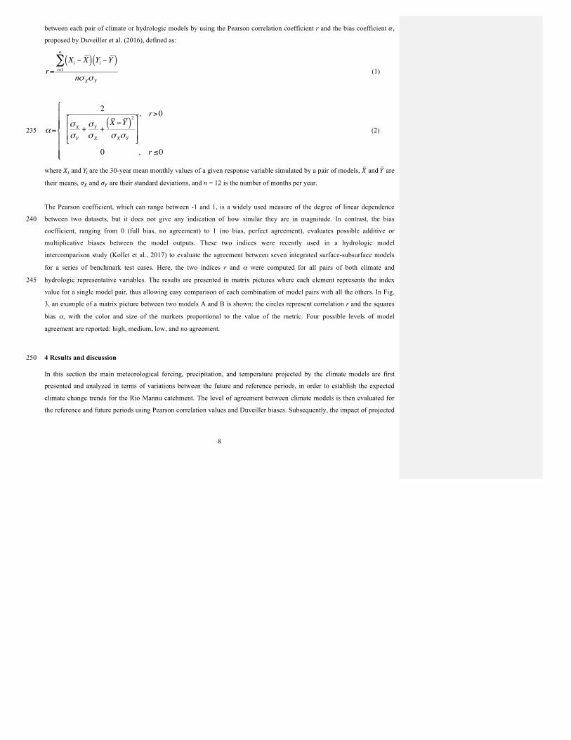
between each pair of climate or hydrologic models by using the Pearson correlation coefficient r and the bias coefficient 𝛼,

proposed by Duveiller et al. (2016), defined as:

r=Xi − X( ) Yi −Y( )

i=1

n

∑nσ XσY

(1)

α=

2

σ X

σY

+σY

σ X

+X −Y( )

2

σ XσY

"

#

$$

%

&

''

, r>0

0 , r ≤0

)

*

+++

,

+++

(2) 235

where 𝑋! and 𝑌! are the 30-year mean monthly values of a given response variable simulated by a pair of models, 𝑋 and 𝑌 are

their means, 𝜎! and 𝜎! are their standard deviations, and n = 12 is the number of months per year.

The Pearson coefficient, which can range between -1 and 1, is a widely used measure of the degree of linear dependence

between two datasets, but it does not give any indication of how similar they are in magnitude. In contrast, the bias 240

coefficient, ranging from 0 (full bias, no agreement) to 1 (no bias, perfect agreement), evaluates possible additive or

multiplicative biases between the model outputs. These two indices were recently used in a hydrologic model

intercomparison study (Kollet et al., 2017) to evaluate the agreement between seven integrated surface-subsurface models

for a series of benchmark test cases. Here, the two indices r and α were computed for all pairs of both climate and

hydrologic representative variables. The results are presented in matrix pictures where each element represents the index 245

value for a single model pair, thus allowing easy comparison of each combination of model pairs with all the others. In Fig.

3, an example of a matrix picture between two models A and B is shown: the circles represent correlation r and the squares

bias α, with the color and size of the markers proportional to the value of the metric. Four possible levels of model

agreement are reported: high, medium, low, and no agreement.

4 Results and discussion 250

In this section the main meteorological forcing, precipitation, and temperature projected by the climate models are first

presented and analyzed in terms of variations between the future and reference periods, in order to establish the expected

climate change trends for the Rio Mannu catchment. The level of agreement between climate models is then evaluated for

the reference and future periods using Pearson correlation values and Duveiller biases. Subsequently, the impact of projected

9

climate change is investigated through application of the five hydrologic models. Water availability and fluxes in terms of 255

discharge, soil water content, and actual evapotranspiration are analyzed for trends and inter-model agreement.

4.1 Climate models: projected changes and comparison/agreement analysis

Climate model outputs were bias-corrected and downscaled to provide more reliable inputs to the hydrologic models.

Specifically, for each climate model, the climatological means of precipitation (P) and temperature (T) averaged over the

catchment were computed at annual and monthly scales. Figure 4 compares results for the reference and future periods. All 260

models predict a decrease of mean annual P, with percent changes ranging from -7 % to -21 %, and an increase of T from 1.9

ºC to 3 ºC. All models predict negative changes in P for all months except winter (December–February), where the models

simulated an increase in P, and also June for ECH-REM and October for ECH-RMO. T is projected to rise in all months for

all models, with the RCMs forced by ECH predicting comparable magnitudes in change, and HCH-RCA simulating the

largest increment. 265

To quantify the agreement of the monthly climatologies of P and T predicted by the models, the correlation coefficient, r,

and the bias, α, are plotted in Fig. 5. The left and right panels show the results for, respectively, P and T for the reference

(top) and future (bottom) periods. In each panel, circles represent r and squares α, while color and size of the markers are

proportional to the metric value. The actual values of the Pearson and bias coefficients are reported in the supplementary 270

Table S1. The metrics indicate a general high level of agreement of the climatologies simulated by all models, with r and α

for each pair of models always larger than 0.9 for both variables and in both periods. Comparing the same climate model for

the reference and future periods, the values of r and α (last row and last column, respectively, of the bottom panels) are also

high for both variables: for P and the HCH-RCA model, which is the model that slightly differs from the others, both

Pearson and bias coefficients are close to 1 (r = 0.918 and α = 0.912). As a result, the agreement of seasonal cycles is high, 275

especially in the case of temperature, suggesting that the uncertainty due to climate models can be considered low, although

a small bias is found when comparing the three climate models forced by ECH with HCH-RCA, as expected since it is

recognized that GCMs exert the major influence on the projected climate change (Graham et al., 2007; Kay et al., 2009).

4.2 Hydrologic impact

A summary of the annual and monthly climatologies of basin-averaged potential evapotranspiration (ETP), runoff (Q), soil 280

water content (SWC), and actual evapotranspiration (ETa) simulated by the five hydrologic models, forced by four climate

models, is reported in Fig. 6-9. Each figure shows: the annual simulated variable in each period, including the percent

change from reference to future (panel a); the relative change in mean annual values between reference and future periods

forced by the four climate models (panel b); the seasonal distribution of mean monthly values of each variable during

Enrica Perra � 30/5/18 11:27Deleted: For285

Enrica Perra � 30/5/18 11:27Deleted: , and in the bottom panels there is also the comparison between the reference and future periods.

10

reference and future periods and corresponding standard deviations (panel c); and finally the seasonal distribution of relative

change of mean monthly values between reference and future periods (panel d). 290

ETP is predicted to rise by all models on an annual basis (Fig. 6a), mostly due to the projected increment of T. The values of

annual and monthly (Fig. 6c) ETP differs among the hydrologic models, due to the different computation methods adopted.

For SWAT and WASIM, ETP was computed at a daily time scale by internal routines based on Hargreaves (Hargreaves et

al., 1994, 2003) and Penman-Monteith (Penman, 1948; Monteith, 1965) formulas, respectively, producing an annual mean of 295

about 1100 mm for SWAT and 1400 mm for WASIM. For CATHY, TOPKAPI, and tRIBS, a common reliable diurnal cycle

for ETP was derived at hourly time scale using an approach based on Penman-Monteith and Hargreaves formulas, detailed in

Mascaro el al. (2013b), producing an annual mean of about 650 mm, which is consistent with previous estimates for this

region (Pulina et al., 1986). From Fig. 6c we can also observe the slight increase of ETP predicted by all hydrologic models

in the future period, except for the WASIM model and especially during summer and spring months. Furthermore, notice 300

that the highest increase of ETP is predicted with all hydrologic models under HCH-RCA forcing (Fig. 6b), as expected

since this GCM-RCM combination also projects the highest increase in temperature, as already discussed. Among the

hydrologic models, WASIM is the one that predicts the higher increase. We can observe also from Fig. 6d that relative

changes in potential evapotranspiration are predicted to increase much more during summer and spring.

305

Results in terms of Q are analyzed in Fig. 7: it is apparent that all models predict decreasing values in the future. Figure 7a,

reporting mean annual Q obtained for each hydrologic model in the reference and future periods obtained as an average

among the four climate models, shows a reduction that ranges from -12 % according to SWAT to -69 % according to

CATHY. Figure 7b reports the relative change between future and reference periods computed for each climate model

configuration: we can observe that the reduction varies within the same hydrologic model considering different climate 310

forcing. The largest decrease is always given by configurations forced with HCH-RCA, ranging from -23 % for the SWAT

model to -91 % for the CATHY model, followed by the climate model ECH-RCA, for which the reduction varies from -16

% for SWAT to -67 % for CATHY. A summary in terms of change (%) between reference and future periods for mean

annual Q, simulated by the five hydrologic models and the four climate models, is provided in Table 3. Figure 7c refers to

mean monthly Q, showing the mean seasonality in reference (solid line) and future (dotted line) periods with bars indicating 315

the standard deviations within each model. Figure 7d details the monthly variations during the two periods according to the

five hydrologic models: the seasonality is quite similar among them even if some differences hold also in this case. The five

hydrologic models predict diminished mean monthly Q in the future period throughout the year with the exception of

January and February, when SWAT and WASIM simulate a slight increase.

320

Figure 8 shows mean values and changes of SWC in the first meter depth of soil. All simulations predict a decreasing trend

of SWC, but again we can notice some differences among the hydrologic models. For instance Fig. 8a clearly shows that

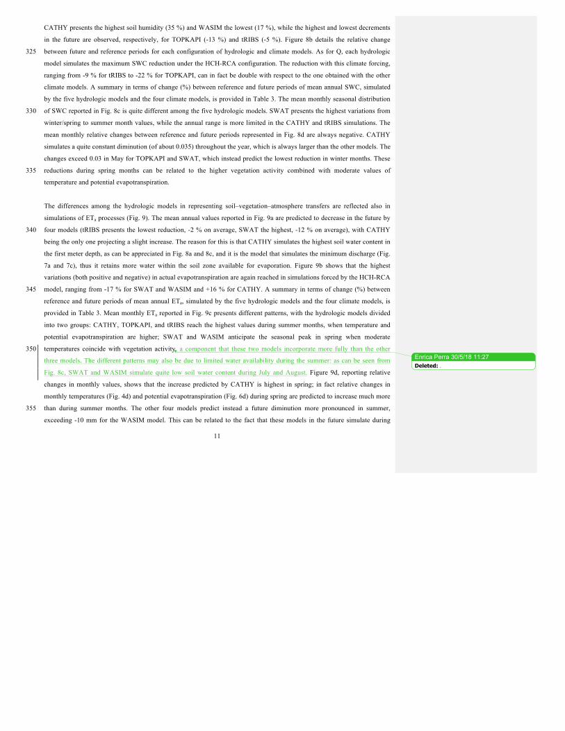
11

CATHY presents the highest soil humidity (35 %) and WASIM the lowest (17 %), while the highest and lowest decrements

in the future are observed, respectively, for TOPKAPI (-13 %) and tRIBS (-5 %). Figure 8b details the relative change

between future and reference periods for each configuration of hydrologic and climate models. As for Q, each hydrologic 325

model simulates the maximum SWC reduction under the HCH-RCA configuration. The reduction with this climate forcing,

ranging from -9 % for tRIBS to -22 % for TOPKAPI, can in fact be double with respect to the one obtained with the other

climate models. A summary in terms of change (%) between reference and future periods of mean annual SWC, simulated

by the five hydrologic models and the four climate models, is provided in Table 3. The mean monthly seasonal distribution

of SWC reported in Fig. 8c is quite different among the five hydrologic models. SWAT presents the highest variations from 330

winter/spring to summer month values, while the annual range is more limited in the CATHY and tRIBS simulations. The

mean monthly relative changes between reference and future periods represented in Fig. 8d are always negative. CATHY

simulates a quite constant diminution (of about 0.035) throughout the year, which is always larger than the other models. The

changes exceed 0.03 in May for TOPKAPI and SWAT, which instead predict the lowest reduction in winter months. These

reductions during spring months can be related to the higher vegetation activity combined with moderate values of 335

temperature and potential evapotranspiration.

The differences among the hydrologic models in representing soil–vegetation–atmosphere transfers are reflected also in

simulations of ETa processes (Fig. 9). The mean annual values reported in Fig. 9a are predicted to decrease in the future by

four models (tRIBS presents the lowest reduction, -2 % on average, SWAT the highest, -12 % on average), with CATHY 340

being the only one projecting a slight increase. The reason for this is that CATHY simulates the highest soil water content in

the first meter depth, as can be appreciated in Fig. 8a and 8c, and it is the model that simulates the minimum discharge (Fig.

7a and 7c), thus it retains more water within the soil zone available for evaporation. Figure 9b shows that the highest

variations (both positive and negative) in actual evapotranspiration are again reached in simulations forced by the HCH-RCA

model, ranging from -17 % for SWAT and WASIM and +16 % for CATHY. A summary in terms of change (%) between 345

reference and future periods of mean annual ETa, simulated by the five hydrologic models and the four climate models, is

provided in Table 3. Mean monthly ETa reported in Fig. 9c presents different patterns, with the hydrologic models divided

into two groups: CATHY, TOPKAPI, and tRIBS reach the highest values during summer months, when temperature and

potential evapotranspiration are higher; SWAT and WASIM anticipate the seasonal peak in spring when moderate

temperatures coincide with vegetation activity, a component that these two models incorporate more fully than the other 350

three models. The different patterns may also be due to limited water availability during the summer: as can be seen from

Fig. 8c, SWAT and WASIM simulate quite low soil water content during July and August. Figure 9d, reporting relative

changes in monthly values, shows that the increase predicted by CATHY is highest in spring; in fact relative changes in

monthly temperatures (Fig. 4d) and potential evapotranspiration (Fig. 6d) during spring are predicted to increase much more

than during summer months. The other four models predict instead a future diminution more pronounced in summer, 355

exceeding -10 mm for the WASIM model. This can be related to the fact that these models in the future simulate during

Enrica Perra � 30/5/18 11:27Deleted: .

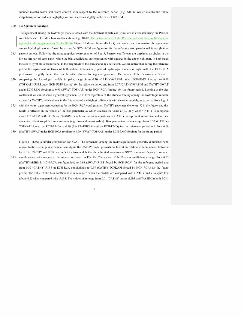
12

summer months lower soil water content with respect to the reference period (Fig. 8d). In winter months the future

evapotranspiration reduces negligibly, or even increases slightly in the case of WASIM.

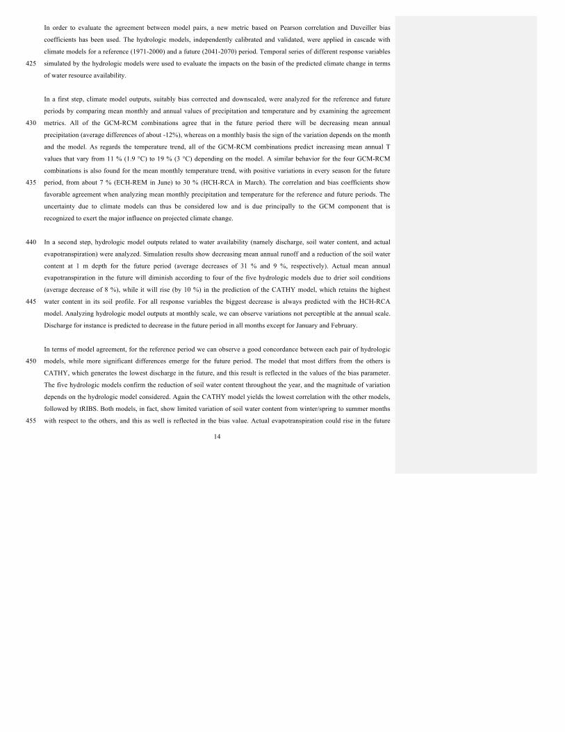
4.3 Agreement analysis 360

The agreement among the hydrologic models forced with the different climate configurations is evaluated using the Pearson

correlation and Duveiller bias coefficients in Fig. 10-12. The actual values of the Pearson and and bias coefficients are

reported in the supplementary Tables S2-S4. Figure 10 shows the results for Q, and each panel summarizes the agreement

among hydrologic models forced by a specific GCM-RCM configuration for the reference (top panels) and future (bottom

panels) periods. Following the same graphical representation of Fig. 3, Pearson coefficients are displayed as circles in the 365

lowest-left part of each panel, while the bias coefficients are represented with squares in the upper-right part. In both cases

the size of symbols is proportional to the magnitude of the corresponding coefficient. We can notice that during the reference

period the agreement in terms of both indices between any pair of hydrologic models is high, with the HCH-RCA

performance slightly better than for the other climate forcing configurations. The values of the Pearson coefficient r,

comparing the hydrologic models in pairs, range from 0.70 (CATHY-WASIM under ECH-RMO forcing) to 0.99 370

(TOPKAPI-tRIBS under ECH-RMO forcing) for the reference period and from 0.67 (CATHY-WASIM and CATHY-SWAT

under ECH-REM forcing) to 0.99 (SWAT-TOPKAPI under HCH-RCA forcing) for the future period. Looking at the bias

coefficient we can observe a general agreement (α > 0.7) regardless of the climate forcing among the hydrologic models,

except for CATHY, which shows in the future period the highest differences with the other models, as expected from Fig. 5,

with the lowest agreement occurring for the HCH-RCA configuration. CATHY generates the lowest Q in the future, and this 375

result is reflected in the values of the bias parameter α, which exceeds the value of 0.7 only when CATHY is compared

under ECH-REM with tRIBS and WASIM, which use the same equations as CATHY to represent subsurface and surface

dynamics, albeit simplified in some way (e.g., lower dimensionality). Bias parameters values range from 0.53 (CATHY-

TOPKAPI forced by ECH-RMO) to 0.99 (SWAT-tRIBS forced by ECH-RMO) for the reference period and from 0.09

(CATHY-SWAT under HCH-RCA forcing) to 0.99 (SWAT-TOPKAPI under ECH-RMO forcing) for the future period. 380

Figure 11 shows a similar comparison for SWC. The agreement among the hydrologic models generally diminishes with

respect to the discharge intercomparison. Again the CATHY model presents the lowest correlation with the others, followed

by tRIBS. CATHY and tRIBS are in fact the two models that show limited variations of SWC from winter/spring to summer

month values with respect to the others, as shown in Fig. 8b. The values of the Pearson coefficient r range from 0.65 385

(CATHY-tRIBS in HCH-RCA configuration) to 0.98 (SWAT-tRIBS forced by ECH-RCA) for the reference period and

from 0.57 (CATHY-tRIBS in ECH-RCA simulations) to 0.97 (CATHY-TOPKAPI forced by HCH-RCA) for the future

period. The value of the bias coefficient α is near zero when the models are compared with CATHY and also quite low

(about 0.2) when compared with tRIBS. The values of α range from 0.01 (CATHY versus tRIBS and WASIM in both ECH-

13

RCA and ECH-REM configurations) to 0.86 (TOPKAPI versus WASIM forced by ECH-RMO) for the reference period and 390

from 0.01 (CATHY-WASIM in ECH-REM simulations) to 0.94 (TOPKAPI versus WASIM forced by ECH-RMO) for the

future period.

The analysis of agreement presents the lowest Pearson correlation values in the case of ETa (Fig. 12). The values of r range

from -0.21 (CATHY-WASIM in ECH-REM configuration) to 0.98 (CATHY-tRIBS for all climate model configurations) for 395

the reference period and from -0.29 (CATHY-WASIM in ECH-REM simulations) to 0.99 (CATHY-tRIBS for all

configurations) for the future period. Despite the high values of the Pearson coefficient between CATHY and tRIBS for both

the reference and future periods regardless of the GCM-RCM forcing, the Duveiller index displays a worsening (α ≈ 0.6 –

0.8). Considering overall results, the values of the bias coefficient α range from 0 (CATHY and tRIBS versus WASIM in

ECH-REM configuration) to 0.99 (TOPKAPI versus tRIBS for all configurations) for the reference period and from 0 400

(CATHY-WASIM in ECH-RMO simulations) to 0.99 (TOPKAPI versus tRIBS for all configurations) for the future period.

From this figure it can be noted that, notwithstanding the differences, Pearson and bias indices for the reference period are

similar for CATHY, tRIBS, and TOPKAPI (which are forced with the same ETP values). Furthermore, these models reach

the highest values of ETa during the summer months (Fig. 9c), when the temperature is highest. For the future period this

agreement is maintained, with a strong correlation between tRIBS and TOPKAPI. Referring to the pair SWAT-WASIM, 405

they anticipate the peak of ETa in spring when moderate temperatures coincide with vegetation activity (Fig. 9c). This can be

seen for the reference period and less for the future one, when α is slightly lower.

The differences that emerge from the analysis of agreement are consistent with the key structural differences between the

hydrologic models. CATHY, for instance, has the most detailed subsurface representation of the five models (fully three-410

dimensional Richards equation; soil and aquifer zones), and as such will tend to retain more water in subsurface storage,

making some of this water available for subsequent evaporation. An additional factor contributing to greater subsurface

storage in CATHY is that all the lateral and bottom boundaries of the simulation domain are considered impermeable. In the

agreement metrics CATHY tends to align most with TOPKAPI and tRIBS, which, although with a more simplified

representation, also account for both vertical and lateral subsurface flow, unlike SWAT and WASIM, which resolve flow 415

only in the vertical direction. These latter two models, on the other hand, show strong agreement, to the exclusion of the

other models, for some of the evapotranspiration responses, consistent with the fact that both these models include a quite

detailed representation of vegetation processes.

5 Conclusions

Five hydrologic models forced with the outputs of four combinations of global and regional climate models were compared 420

to evaluate climate change consequences on the response of a medium-sized Mediterranean basin, the Rio Mannu catchment.

Enrica Perra � 30/5/18 11:27Moved (insertion) [1]

Enrica Perra � 30/5/18 11:27Moved (insertion) [2]

14

In order to evaluate the agreement between model pairs, a new metric based on Pearson correlation and Duveiller bias

coefficients has been used. The hydrologic models, independently calibrated and validated, were applied in cascade with

climate models for a reference (1971-2000) and a future (2041-2070) period. Temporal series of different response variables

simulated by the hydrologic models were used to evaluate the impacts on the basin of the predicted climate change in terms 425

of water resource availability.

In a first step, climate model outputs, suitably bias corrected and downscaled, were analyzed for the reference and future

periods by comparing mean monthly and annual values of precipitation and temperature and by examining the agreement

metrics. All of the GCM-RCM combinations agree that in the future period there will be decreasing mean annual 430

precipitation (average differences of about -12%), whereas on a monthly basis the sign of the variation depends on the month

and the model. As regards the temperature trend, all of the GCM-RCM combinations predict increasing mean annual T

values that vary from 11 % (1.9 °C) to 19 % (3 °C) depending on the model. A similar behavior for the four GCM-RCM

combinations is also found for the mean monthly temperature trend, with positive variations in every season for the future

period, from about 7 % (ECH-REM in June) to 30 % (HCH-RCA in March). The correlation and bias coefficients show 435

favorable agreement when analyzing mean monthly precipitation and temperature for the reference and future periods. The

uncertainty due to climate models can thus be considered low and is due principally to the GCM component that is

recognized to exert the major influence on projected climate change.

In a second step, hydrologic model outputs related to water availability (namely discharge, soil water content, and actual 440

evapotranspiration) were analyzed. Simulation results show decreasing mean annual runoff and a reduction of the soil water

content at 1 m depth for the future period (average decreases of 31 % and 9 %, respectively). Actual mean annual

evapotranspiration in the future will diminish according to four of the five hydrologic models due to drier soil conditions

(average decrease of 8 %), while it will rise (by 10 %) in the prediction of the CATHY model, which retains the highest

water content in its soil profile. For all response variables the biggest decrease is always predicted with the HCH-RCA 445

model. Analyzing hydrologic model outputs at monthly scale, we can observe variations not perceptible at the annual scale.

Discharge for instance is predicted to decrease in the future period in all months except for January and February.

In terms of model agreement, for the reference period we can observe a good concordance between each pair of hydrologic

models, while more significant differences emerge for the future period. The model that most differs from the others is 450

CATHY, which generates the lowest discharge in the future, and this result is reflected in the values of the bias parameter.

The five hydrologic models confirm the reduction of soil water content throughout the year, and the magnitude of variation

depends on the hydrologic model considered. Again the CATHY model yields the lowest correlation with the other models,

followed by tRIBS. Both models, in fact, show limited variation of soil water content from winter/spring to summer months

with respect to the others, and this as well is reflected in the bias value. Actual evapotranspiration could rise in the future 455

15

period according to the CATHY model and, during January and February, also according to WASIM, which instead predicts

the strongest reductions in summer months. As regards the analysis of agreement for actual evapotranspiration, Pearson and

bias indices are similar for CATHY, tRIBS, and TOPKAPI (which are forced with the same values of potential

evapotranspiration). Moreover, these models reach the highest values of actual evapotranspiration during summer months.

For the future period this agreement is maintained, with a strong correlation between tRIBS and TOPKAPI. The model pair 460

SWAT-WASIM anticipates the peak of actual evapotranspiration in spring when moderate temperatures coincide with

vegetation activity. This behavior is more pronounced for the reference period than for the future one, due to the higher bias.

Overall the five hydrologic models show good agreement, responding similarly to the climate model predictions of reduced

precipitation and increased temperatures and lending strong support to a future scenario of increased water shortages for this

region of the Mediterranean, with negative consequences especially for the agricultural sector. 465

Acknowledgements

This study was begun within the CLIMB project (Climate Induced Changes on the Hydrology of Mediterranean Basins,

http://www.climb-fp7.eu), funded by the European Commission 7th Framework Programme. Financial support was also

provided by the Sardinia Region L.R. 7/2007 projects “Valutazione degli impatti sul comportamento idrologico dei bacini

idrografici e sulle produzioni agricole conseguenti alle condizioni di cambiamento climatico” (funding call 2008) and 470

“Impatti antropogenici e climatici sul ciclo idrologico a scala di bacino e di versante” (funding call 2013). The authors wish

to thank Gabriele Coccia for his help in implementing the TOPKAPI model. The first author gratefully acknowledges the

Sardinia Regional Government for financial support during her PhD (P.O.R. Sardegna F.S.E. Operational Programme of the

Autonomous Region of Sardinia, European Social Fund 2007-2013 - Axis IV Human Resources, Objective l.3, Line of

Activity l.3.1). 475

References

Acero, F. J., García, J. A., Cruz Gallego, M., Parey, S. and Dacunha-Castelle, D.: Trends in summer extreme temperatures

over the Iberian Peninsula using nonurban station data, J. Geophys. Res. Atmos. J. Geophys. Res. Atmos, 119(119), 39–53,

doi:10.1002/2013JD020590, 1002.

Arnold, J. G., Srinivasan, R., Muttiah, R. S. and Williams, J. R.: Large area hydrologic modeling and assessment part I: 480

model development, J. Am. Water Resour. Assoc., 34(1), 73–89, doi:10.1111/j.1752-1688.1998.tb05961.x, 1998.

Arnold, J. G., Srinivasan, R., Muttiah, R. S. and Allen, P. M.: Continental scale simulation of the hydrologic balance, J. Am.

Water Resour. Assoc., 35(5), 1037–1051, doi:10.1111/j.1752-1688.1999.tb04192.x, 1999.

Bae, D.-H., Jung, I.-W. and Lettenmaier, D. P.: Hydrologic uncertainties in climate change from IPCC AR4 GCM

simulations of the Chungju Basin, Korea, J. Hydrol., 401(1–2), 90–105, doi:10.1016/J.JHYDROL.2011.02.012, 2011. 485

Enrica Perra � 30/5/18 11:27Moved up [1]: The differences that emerge from the analysis of agreement are consistent with the key structural differences between the hydrologic models. CATHY, for instance, has the most detailed subsurface representation of the five models (fully 490 three-dimensional Richards equation; soil and aquifer zones), and as such will tend to retain more water in subsurface storage, making some of this water available for subsequent evaporation.

Enrica Perra � 30/5/18 11:27Moved up [2]: In the agreement metrics CATHY 495 tends to align most with TOPKAPI and tRIBS, which, although with a more simplified representation, also account for both vertical and lateral subsurface flow, unlike SWAT and WASIM, which resolve flow only in the vertical direction. 500 These latter two models, on the other hand, show strong agreement, to the exclusion of the other models, for some of the evapotranspiration responses, consistent with the fact that both these models include a quite detailed representation of 505 vegetation processes.

Enrica Perra � 30/5/18 11:27Deleted: Notwithstanding these differences, over

16

Bartholmes, J. and Todini, E.: Coupling meteorological and hydrological models for flood forecasting, Hydrol. Earth Syst.

Sci., 9(4), 333–346, 2005.

Bastola, S., Murphy, C. and Sweeney, J.: The role of hydrological modelling uncertainties in climate change impact 510

assessments of Irish river catchments, Adv. Water Resour., 34(5), 562–576, doi:10.1016/j.advwatres.2011.01.008, 2011.

Bosshard, T., Carambia, M., Goergen, K., Kotlarski, S., Krahe, P., Zappa, M. and Schär, C.: Quantifying uncertainty sources

in an ensemble of hydrological climate-impact projections, Water Resour. Res., 49(3), 1523–1536,

doi:10.1029/2011WR011533, 2013.

Camporese, M., Paniconi, C., Putti, M. and Orlandini, S.: Surface-subsurface flow modeling with path-based runoff routing, 515

boundary condition-based coupling, and assimilation of multisource observation data, Water Resour. Res., 46(2),

doi:10.1029/2008WR007536, 2010.

Cassiani, G., Ursino, N., Deiana, R., Vignoli, G., Boaga, J., Rossi, M., Perri, M. T., Blaschek, M., Duttmann, R., Meyer, S.,

Cau, P., Cadeddu, A., Gallo, C., Lecca, G., and Marrocu, M.: Estimating the water balance of the Sardinian island using the

SWAT model, L’Acqua, 5, 29–38, 2005. 520

Ciarapica, L. and Todini, E.: TOPKAPI: a model for the representation of the rainfall-runoff process at different scales,

Hydrol. Process., 16(2), 207–229, doi:10.1002/hyp.342, 2002.

Clark, M. P., Slater, A. G., Rupp, D. E., Woods, R. A., Vrugt, J. A., Gupta, H. V., Wagener, T. and Hay, L. E.: Framework

for Understanding Structural Errors (FUSE): A modular framework to diagnose differences between hydrological models,

Water Resour. Res., 44(12), doi:10.1029/2007WR006735, 2008. 525

Cornelissen, T., Diekkrüger, B. and Giertz, S.: A comparison of hydrological models for assessing the impact of land use and

climate change on discharge in a tropical catchment, J. Hydrol., 498, 221–236, doi:10.1016/J.JHYDROL.2013.06.016, 2013.

Dams, J., Nossent, J., Senbeta, T. B., Willems, P. and Batelaan, O.: Multi-model approach to assess the impact of climate

change on runoff, J. Hydrol., 529, 1601–1616, doi:10.1016/J.JHYDROL.2015.08.023, 2015.

Deidda, R.: Rainfall downscaling in a space-time multifractal framework, Water Resour. Res., 36(7), 1779–1794, 530

doi:10.1029/2000WR900038, 2000.

Deidda, R., Benzi, R. and Siccardi, F.: Multifractal modeling of anomalous scaling laws in rainfall, WATER Resour. Res.,

35(6), 1853–1867, doi:10.1029/1999WR900036, 1999.

Deidda, R., Marrocu, M., Caroletti, G., Pusceddu, G., Langousis, A., Lucarini, V., Puliga, M. and Speranza, A.: Regional

climate models' performance in representing precipitation and temperature over selected Mediterranean areas, Hydrol. Earth 535

Syst. Sci., 17, 5041–5059, doi:10.5194/hess-17-5041-2013, 2013.

Duveiller, G., Fasbender, D. and Meroni, M.: Revisiting the concept of a symmetric index of agreement for continuous

datasets, Sci. Rep., 6(1), 19401, doi:10.1038/srep19401, 2016.

Filion, R., Bernier, M., Paniconi, C., Chokmani, K., Melis, M., Soddu, A., Talazac, M. and Lafortune, F.-X.: Remote sensing

for mapping soil moisture and drainage potential in semi-arid regions: Applications to the Campidano plain of Sardinia, 540

Italy, Sci. Total Environ., 543(Pt B), 862–876, doi:10.1016/j.scitotenv.2015.07.068, 2016.

Enrica Perra � 30/5/18 11:27Deleted: Briggs, D.J., and Martin, D.: CORINE: an environmental information system for the European Community, European Environ. Rev., 2, 29–34, 1988. 545

Enrica Perra � 30/5/18 11:27Deleted: Climate model validation and selection for hydrological applications

Enrica Perra � 30/5/18 11:27Deleted: representative

Enrica Perra � 30/5/18 11:27Deleted: catchments

Enrica Perra � 30/5/18 11:27Deleted: . Discuss., 10(7), 9105–9145550 Enrica Perra � 30/5/18 11:27Deleted: hessd-10-9105

17

Gädeke, A., Hölzel, H., Koch, H., Pohle, I. and Grünewald, U.: Analysis of uncertainties in the hydrological response of a

model-based climate change impact assessment in a subcatchment of the Spree River, Germany, Hydrol. Process., 28(12),

3978–3998, doi:10.1002/hyp.9933, 2014.

Gatel, L., Lauvernet, C., Carluer, N. and Paniconi, C.: Effect of surface and subsurface heterogeneity on the hydrological 555

response of a grassed buffer zone, J. Hydrol., 542, 637–647, doi:10.1016/J.JHYDROL.2016.09.038, 2016.

Gauthier, M. J., Camporese, M., Rivard, C., Paniconi, C. and Larocque, M.: A modeling study of heterogeneity and surface

water-groundwater interactions in the Thomas Brook catchment, Annapolis Valley (Nova Scotia, Canada), Hydrol. Earth

Syst. Sci, 13, 1583–1596, 2009.

Giorgi, F.: Climate change hot-spots, Geophys. Res. Lett., 33(8), L08707, doi:10.1029/2006GL025734, 2006. 560

Giorgi, F. and Lionello, P.: Climate change projections for the Mediterranean region, Glob. Planet. Change, 63(2–3), 90–

104, doi:10.1016/j.gloplacha.2007.09.005, 2008.

Giorgi, F. and Mearns, L. O.: Calculation of average, uncertainty range, and reliability of regional climate changes from

AOGCM simulations via the “Reliability Ensemble Averaging” (REA) method, J. Clim., 15(10), 1141–1158,

doi:10.1175/1520-0442(2002)015<1141:COAURA>2.0.CO;2, 2002. 565

Graham, L. P., Hagemann, S., Jaun, S. and Beniston, M.: On interpreting hydrological change from regional climate models,

Clim. Change, 81(SUPPL. 1), 97–122, doi:10.1007/s10584-006-9217-0, 2007.

Hargreaves, G. H.: Defining and Using Reference Evapotranspiration, J. Irrig. Drain. Eng., 120(6), 1132–1139,

doi:10.1061/(ASCE)0733-9437(1994)120:6(1132), 1994.

Hargreaves, G. H. and Allen, R. G.: History and Evaluation of Hargreaves Evapotranspiration Equation, J. Irrig. Drain. Eng., 570

129(1), 53–63, doi:10.1061/(ASCE)0733-9437(2003)129:1(53), 2003.

Hawkins, E. and Sutton, R.: The potential to narrow uncertainty in regional climate predictions, Bull. Am. Meteorol. Soc.,

90(8), 1095–1107, doi:10.1175/2009BAMS2607.1, 2009.

Hawkins, G. A., Vivoni, E. R., Robles-Morua, A., Mascaro, G., Rivera, E. and Dominguez, F.: A climate change projection

for summer hydrologic conditions in a semiarid watershed of central Arizona, J. Arid Environ., 118, 9–20, 575

doi:10.1016/j.jaridenv.2015.02.022, 2015.

Haylock, M. R., Hofstra, N., Klein Tank, A. M. G., Klok, E. J., Jones, P. D. and New, M.: A European daily high-resolution

gridded data set of surface temperature and precipitation for 1950–2006, J. Geophys. Res, 113, doi:10.1029/2008JD010201,

2008.

Im, E.-S., Jung, I.-W., Chang, H., Bae, D.-H. and Kwon, W.-T.: Hydroclimatological response to dynamically downscaled 580

climate change simulations for Korean basins, Clim. Change, 100(3–4), 485–508, doi:10.1007/s10584-009-9691-2, 2010.

IPCC, Climate Change: Impacts, Adaptation, and Vulnerability. Part A: Global and Sectoral Aspects. Contribution of

Working Group II to the Fifth Assessment Report of the Intergovernmental Panel on Climate Change [Field, C.B., Barros,

V.R., Dokken, D.J., Mach, K.J., Mastrandrea, M.D., Bilir, T.E., Chatterjee, M., Ebi, K.L., Estrada, Y.O., Genova, R.C.,

18

Girma, B., Kissel, E.S., Levy, A.N., MacCracken, S., Mastrandrea, P.R., White L.L. (eds.)], Cambridge University Press, 585

Cambridge, United Kingdom and New York, NY, USA, 1132 pp, 2014.

Ivanov, V. Y., Vivoni, E. R., Bras, R. L. and Entekhabi, D.: Catchment hydrologic response with a fully distributed

triangulated irregular network model, Water Resour. Res, 40, doi:10.1029/2004WR003218, 2004.

Jasper, K., Gurtz, J. and Lang, H.: Advanced flood forecasting in Alpine watersheds by coupling meteorological

observations and forecasts with a distributed hydrological model, J. Hydrol., 267(1–2), 40–52, doi:10.1016/S0022-590

1694(02)00138-5, 2002.

Jiang, L. and Islam, S.: A methodology for estimation of surface evapotranspiration over large areas using remote sensing

observations, Geophys. Res. Lett., 26(17), 2773–2776, doi:10.1029/1999GL006049, 1999.

Jiang, T., Chen, Y. D., Xu, C., Chen, X., Chen, X. and Singh, V. P.: Comparison of hydrological impacts of climate change

simulated by six hydrological models in the Dongjiang Basin, South China, J. Hydrol., 336(3–4), 316–333, 595

doi:10.1016/J.JHYDROL.2007.01.010, 2007.

Kay, A. L., Davies, H. N., Bell, V. A. and Jones, R. G.: Comparison of uncertainty sources for climate change impacts: flood

frequency in England, Clim. Change, 92(1–2), 41–63, doi:10.1007/s10584-008-9471-4, 2009.

El Kenawy, A., López-Moreno, J. I. and Vicente-Serrano, S. M.: Recent trends in daily temperature extremes over

northeastern Spain (1960–2006), Nat. Hazards Earth Syst. Sci., 11(9), 2583–2603, doi:10.5194/nhess-11-2583-2011, 2011. 600

Kollet, S., Sulis, M., Maxwell, R. M., Paniconi, C., Putti, M., Bertoldi, G., Coon, E. T., Cordano, E., Endrizzi, S., Kikinzon,

E., Mouche, E., Mügler, C., Park, Y.-J., Refsgaard, J. C., Stisen, S. and Sudicky, E.: The integrated hydrologic model

intercomparison project, IH-MIP2: A second set of benchmark results to diagnose integrated hydrology and feedbacks,

Water Resour. Res., 53(1), 867–890, doi:10.1002/2016WR019191, 2017.

Kunstmann, H., Krause, J. and Mayr, S.: Inverse distributed hydrological modelling of Alpine catchments, Hydrol. Earth 605

Syst. Sci, 10, 395–412, 2006.

Liston, G. E., Elder, K., Liston, G. E. and Elder, K.: A Meteorological Distribution System for High-Resolution Terrestrial

Modeling (MicroMet), J. Hydrometeorol., 7(2), 217–234, doi:10.1175/JHM486.1, 2006.

Liu, Z. and Todini, E.: Towards a comprehensive physically-based rainfall-runoff model, Hydrol. Earth Syst. Sci., 6(5), 859–

881, 2002. 610

Liu, Z., Martina, M. L. V. and Todini, E.: Flood forecasting using a fully distributed model: application of the TOPKAPI

model to the Upper Xixian Catchment, Hydrol. Earth Syst. Sci., 9(4), 347–364, 2005.

Liuzzo, L., Noto, L. V., Vivoni, E. R. and La Loggia, G.: Basin-Scale Water Resources Assessment in Oklahoma under

Synthetic Climate Change Scenarios Using a Fully Distributed Hydrologic Model, J. Hydrol. Eng., 15(2), 107–122,

doi:10.1061/(ASCE)HE.1943-5584.0000166, 2010. 615

Ludwig, R., Soddu, A., Duttmann, R., Baghdadi, N., Benabdallah, S., Deidda, R., Marrocu, M., Strunz, G., Wendland, F.,

Engin, G., Paniconi, C., Prettenthaler, F., Lajeunesse, I., Afifi, S., Cassiani, G., Bellin, A., Mabrouk, B., Bach, H., and

Enrica Perra � 30/5/18 11:27Deleted: . Discuss

19

Ammerl, T.: Climate-induced changes on the hydrology of Mediterranean basins - A research concept to reduce uncertainty

and quantify risk, Fresenius Envir. Bull., 19 (10 A), 2379–2384, 2010. 620

Mahmood, T. H. and Vivoni, E. R.: Forest ecohydrological response to bimodal precipitation during contrasting winter to

summer transitions, Ecohydrology, 7(3), 998–1013, doi:10.1002/eco.1424, 2014.

Majone, B., Villa, F., Deidda, R. and Bellin, A.: Impact of climate change and water use policies on hydropower potential in

the south-eastern Alpine region., Sci. Total Environ., 543(Pt B), 965–80, doi:10.1016/j.scitotenv.2015.05.009, 2016.

Marras, P., Muroni, D., Manca, S., Soru, C., Pusceddu, G., Marrocu, M., and Cau, P.: The SWAT model and a web-based 625

information system to assess the water balance of Sardinia (Italy). SWAT International Conference, Pernambuco, Brazil, 21–

33, 2014.

Martina, M. L. V, Todini, E. and Libralon, A.: A Bayesian decision approach to rainfall thresholds based flood warning,

Hydrol. Earth Syst. Sci, 10, 413–426, 2006.

Mascaro, G., Vivoni, E. R. and Deidda, R.: Implications of ensemble quantitative precipitation forecast errors on distributed 630

streamflow forecasting, J. Hydrometeorol., 11(1), 69–86, doi:10.1175/2009JHM1144.1, 2010.

Mascaro, G., Deidda, R. and Hellies, M.: On the nature of rainfall intermittency as revealed by different metrics and

sampling approaches, Hydrol. Earth Syst. Sci., 17(1), 355–369, doi:10.5194/hess-17-355-2013, 2013a.

Mascaro, G., Piras, M., Deidda, R. and Vivoni, E. R.: Distributed hydrologic modeling of a sparsely monitored basin in

Sardinia, Italy, through hydrometeorological downscaling, Hydrol. Earth Syst. Sci., 17(10), 4143–4158, doi:10.5194/hess-635

17-4143-2013, 2013b.

Mascaro, G., Vivoni, E. R. and Méndez-Barroso, L. A.: Hyperresolution hydrologic modeling in a regional watershed and its

interpretation using empirical orthogonal functions, Adv. Water Resour., 83, 190–206, doi:10.1016/j.advwatres.2015.05.023,

2015.

Maurer, E. P. and Hidalgo, H. G.: Utility of daily vs. monthly large-scale climate data: an intercomparison of two statistical 640

downscaling methods, Hydrol. Earth Syst. Sci., 12(2), 551–563, doi:10.5194/hess-12-551-2008, 2008.

Maurer, E. P., Brekke, L. D. and Pruitt, T.: Contrasting Lumped and Distributed Hydrology Models for Estimating Climate

Change Impacts on California Watersheds1, JAWRA J. Am. Water Resour. Assoc., 46(5), 1024–1035, doi:10.1111/j.1752-

1688.2010.00473.x, 2010.

Mausbach, M.J., and Dedrick, A.R.: The length we go: Measuring environmental benefits of conservation practices, J. Soil 645

Water Conserv., 59(5), 96A–103A, 2004.

Meyer, S., Blaschek, M. and Duttmann, R.: Improved hydrological model parametrization for climate change impact

assessment under data scarcity — The potential of field monitoring techniques and geostatistics, Sci. Total Environ., 543,

906–923, doi:10.1016/J.SCITOTENV.2015.07.116, 2016.

Monteith, J. L.: Evaporation and environment., Symp. Soc. Exp. Biol., 19, 205–34, 1965. 650

Najafi, M. R., Moradkhani, H. and Jung, I. W.: Assessing the uncertainties of hydrologic model selection in climate change

impact studies, Hydrol. Process., 25(18), 2814–2826, doi:10.1002/hyp.8043, 2011.

Enrica Perra � 30/5/18 11:27Deleted: Ensemble Quantitative Precipitation Forecast Errors

Enrica Perra � 30/5/18 11:27Deleted: Distributed Streamflow Forecasting, J.655 Enrica Perra � 30/5/18 11:27Moved (insertion) [3]

Enrica Perra � 30/5/18 11:27Deleted: 2013a.

Enrica Perra � 30/5/18 11:27Deleted: Mascaro, G.,

Enrica Perra � 30/5/18 11:27Moved up [3]: Deidda, R. and Hellies, M.: On the nature of rainfall intermittency as revealed by different metrics and sampling approaches, Hydrol. 660 Earth Syst. Sci., 17(1), 355–369, doi:10.5194/hess-17-355-2013,

Enrica Perra � 30/5/18 11:27Deleted: 2013b.

20

Nakićeović, N., Alcamo, J., Davis, G., de Vries, H.J.M., Fenhann, J., Gaffin, S., Gregory, K., Grubler, A., Jung, T.Y., Kram,

T., La Rovere, E.L., Michaelis, L., Mori, S., Morita, T., Papper, W., Pitcher, H., Price, L., Riahi, K., Roehrl, A., Rogner, H-665

H, Sankovski, A., Schlesinger, M., Shukla, P., Smith, S., Swart, R., van Rooijen, S., Victor, N., Dadi, Z.: Emissions

Scenarios, A Special Report of Working Group III of the Intergovernmental Panel on Climate Change. Cambridge

University Press: Cambridge, 559, 2000.

Orlandini, S. and Rosso, R.: Diffusion Wave Modeling of Distributed Catchment Dynamics, J. Hydrol. Eng., 1(3), 103–113,

doi:10.1061/(ASCE)1084-0699(1996)1:3(103), 1996. 670

Paniconi, C. and Wood, E. F.: A detailed model for simulation of catchment scale subsurface hydrologic processes, Water

Resour. Res., 29(6), 1601–1620, doi:10.1029/92WR02333, 1993.

Pechlivanidis, I. G., Arheimer, B., Donnelly, C., Hundecha, Y., Huang, S., Aich, V., Samaniego, L., Eisner, S. and Shi, P.:

Analysis of hydrological extremes at different hydro-climatic regimes under present and future conditions, Clim. Change,

141, 467–481, doi:10.1007/s10584-016-1723-0, 2017. 675

Penman, H. L.: Natural evaporation from open water, hare soil and grass., Proc. R. Soc. Lond. A. Math. Phys. Sci.,

193(1032), 120–45, doi:10.1098/RSPA.1948.0037, 1948.

Piras, M.: Evaluation of climate change impacts on the hydrologic response of a sparsely-monitored basin in Sardinia, Italy,

through distributed hydrologic simulations and hydrometeorological downscaling. PhD Thesis, University of Cagliari, Italy,

2014. 680

Piras, M., Mascaro, G., Deidda, R. and Vivoni, E. R.: Quantification of hydrologic impacts of climate change in a

Mediterranean basin in Sardinia, Italy, through high-resolution simulations, Hydrol. Earth Syst. Sci, 18, 5201–5217,

doi:10.5194/hess-18-5201-2014, 2014.

Pulina, M.A.: L’evapotraspirazione potenziale in Sardegna in funzione dello studio del regime idrico dei suoli. Studi

Sassaresi, Annali della Facoltà di Agraria dell’Università di Sassari, 1986. 685

Schulla, J.: Hydrologische Modellierung von Flussgebieten zur Abschatzung der Folgen von Klimaanderungen. Zurcher

Geographische Schriften, Heft 69, ETH Zurich, pp. 187, 1997.

Schulla, J.: Model description WaSiM (Water balance Simulation Model). Hydrology Software Consulting,

Regensdorferstrasse, Zurich, 2015.

Schulla, J., and Jasper, K.: Model Description WASIM-ETH (Water Balance Simulation Model ETH), ETH-Zurich, Zurich, 690

2001.

Río, S. del, Herrero, L., Fraile, R. and Penas, A.: Spatial distribution of recent rainfall trends in Spain (1961-2006), Int. J.

Climatol., 31(5), 656–667, doi:10.1002/joc.2111, 2011.

Scudeler, C., Paniconi, C., Pasetto, D. and Putti, M.: Examination of the seepage face boundary condition in subsurface and

coupled surface/subsurface hydrological models, Water Resour. Res., 53(3), 1799–1819, doi:10.1002/2016WR019277, 695

2017.

Sousa, P. M., Trigo, R. M., Aizpurua, P., Nieto, R., Gimeno, L. and Garcia-Herrera, R.: Trends and extremes of drought

21

indices throughout the 20th century in the Mediterranean, Nat. Hazards Earth Syst. Sci., 11(1), 33–51, doi:10.5194/nhess-11-

33-2011, 2011.

Sulis, M., Paniconi, C., Rivard, C., Harvey, R. and Chaumont, D.: Assessment of climate change impacts at the catchment 700

scale with a detailed hydrological model of surface-subsurface interactions and comparison with a land surface model, Water

Resour. Res., 47(1), doi:10.1029/2010WR009167, 2011.

Sulis, M., Paniconi, C., Marrocu, M., Huard, D. and Chaumont, D.: Hydrologic response to multimodel climate output using

a physically based model of groundwater/surface water interactions, Water Resour. Res., 48(12),

doi:10.1029/2012WR012304, 2012. 705

Tebaldi, C., Smith, R. L., Nychka, D. and Mearns, L. O.: Quantifying uncertainty in projections of regional climate change:

A Bayesian approach to the analysis of multimodel ensembles, J. Clim., 18(10), 1524–1540, doi:10.1175/JCLI3363.1, 2005.

Thompson, J. R., Green, A. J., Kingston, D. G. and Gosling, S. N.: Assessment of uncertainty in river flow projections for

the Mekong River using multiple GCMs and hydrological models, J. Hydrol., 486, 1–30, doi:10.1016/j.jhydrol.2013.01.029,

2013. 710

van der Linden, P. and Mitchell, J. F. B.: ENSEMBLES: Climate change and its impacts: Summary of research and results

from the ENSEMBLES project, Met Office Hadley Centre, Exeter, UK, 2009.

Vansteenkiste, T., Tavakoli, M., Ntegeka, V., De Smedt, F., Batelaan, O., Pereira, F. and Willems, P.: Intercomparison of

hydrological model structures and calibration approaches in climate scenario impact projections, J. Hydrol., 519, 743–755,

doi:10.1016/J.JHYDROL.2014.07.062, 2014. 715

Volk, M., Hirschfeld, J., Schmidt, G., Bohn, C., Dehnhardt, A., Liersch, S. and Lymburner, L.: A SDSS-based Ecological-

economic Modelling Approach for Integrated River Basin Management on Different Scale Levels – The Project

FLUMAGIS, Water Resour. Manag., 21(12), 2049–2061, doi:10.1007/s11269-007-9158-z, 2007.

Wood, A. W., Leung, L. R., Sridhar, V. and Lettenmaier, D. P.: Hydrologic Implications of Dynamical and Statistical

Approaches to Downscaling Climate Model Outputs, Clim. Change, 62(1–3), 189–216, 720

doi:10.1023/B:CLIM.0000013685.99609.9e, 2004.

Xoplaki, E., González-Rouco, J. F., Luterbacher, J. and Wanner, H.: Mediterranean summer air temperature variability and

its connection to the large-scale atmospheric circulation and SSTs, Clim. Dyn., 20(7–8), 723–739, doi:10.1007/s00382-003-

0304-x, 2003.

Xu, C., Widén, E. and Halldin, S.: Modelling hydrological consequences of climate change—Progress and challenges, Adv. 725

Atmos. Sci., 22(6), 789–797, doi:10.1007/BF02918679, 2005.

Xu, C.-Y. and Singh, V. P.: Review on Regional Water Resources Assessment Models under Stationary and Changing

Climate, Water Resour. Manag., 18(6), 591–612, doi:10.1007/s11269-004-9130-0, 2004.

730

Enrica Perra � 30/5/18 11:27Formatted: English (US)Enrica Perra � 30/5/18 11:27Deleted: ... [1]

Enrica Perra � 30/5/18 11:27Formatted: Font:10 pt

22

Model Discretization

scheme

Infiltration/Subsurface

flow

Surface

flow

Topographic

representation

CATHY Finite element Richards’ equation

Diffusive wave Regular grid

SWAT Subwatershed Tipping bucket Soil Conservation

Service (SCS)

Homogeneous

hydrologic units

TOPKAPI

Finite difference

Kinematic wave

Kinematic wave

Regular grid

tRIBS

Finite difference

control volume

Modified

Green-Ampt

Kinematic wave

Triangulated irregular

network

WASIM Finite difference Richards’ equation

Kinematic wave Regular grid

735 Table 1: Comparison of the structure and characteristics of the five hydrologic models.

740

745

750

23

Climatological center and model Acronym

GCM

Hadley Centre for Climate Prediction, Met Office, UK

HadCM3 Model HCH

Max Planck Institute for Meteorology, Germany

ECHAM5 / MPI Model ECH

RCM

Swedish Meteorological and Hydrological Institute (SMHI), Sweden

RCA Model RCA

Max Planck Institute for Meteorology, Hamburg, Germany

REMO Model REM

Koninklijk Nederlands Meteorologisch Instituut (KNMI), Netherlands

RACMO2 Model RMO

Table 2: List of global and regional climate models used in this work. The four GCM-RCM combinations used are ECH-RCA, 755 ECH-REM, ECH-RMO, and HCH-RCA.

760

765

770

775

24

Overall tendencies

considering all climate models

Overall tendencies

considering all hydrologic models

CAT

(%)

SWA

(%)

TOP

(%)

TRI

(%)

WAS

(%)

ALL

H.M.

(%)

ERC

(%)

ERE

(%)

ERM

(%)

HRC

(%)

ALL

C.M.

(%)

Q 𝜇 -68 -12 -25 -32 -19 -31 -32 -19 -24 -49 -31

𝜎 18 10 13 14 14 14 20 16 26 25 22

SWC 𝜇 -10 -8 -13 -5 -10 -9 -8 -6 -6 -16 -9

𝜎 5 5 6 3 4 5 2 2 3 5 3

ETa 𝜇 10 -12 -8 -2 -11 -5 -3 -3 -5 -7 -5

𝜎 4 5 3 1 5 3 7 6 9 14 9

Table 3: Change (%) between future and reference periods of mean annual discharge (Q), soil water content (SWC) and actual

evapotranspiration (ETa) for the five hydrologic models (CAT = CATHY, SWA = SWAT, TOP = TOPKAPI, TRI = tRIBS, WAS =

WASIM), expressed as mean (𝝁) and standard deviation (𝝈) calculated for each and then all hydrologic models (H.M.) considering 780 all climate models (ERC = ECH-RCA, ERE = ECH-REM, ERM = ECH-RMO, HRC = HCH-RCA), and for each and then all

climate models (C.M.) considering all hydrologic models.

785

790

795

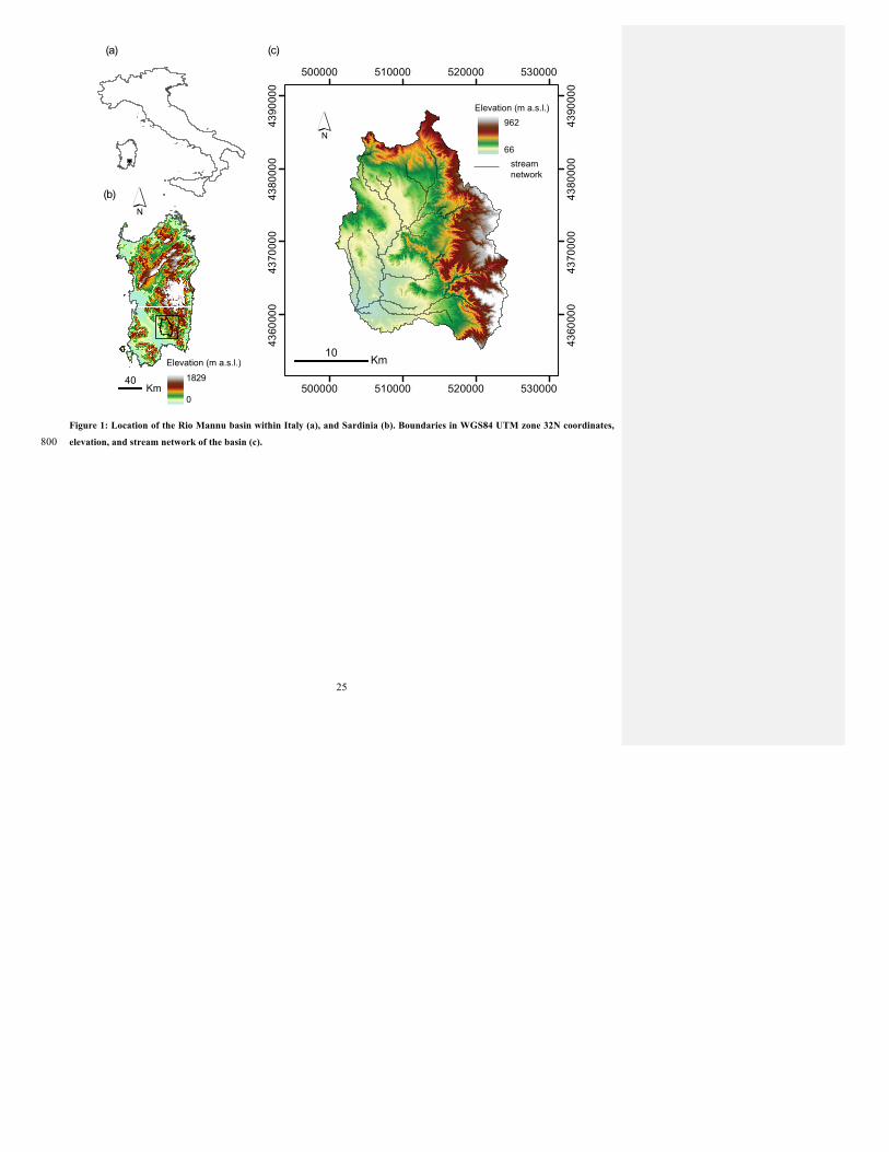
25

Figure 1: Location of the Rio Mannu basin within Italy (a), and Sardinia (b). Boundaries in WGS84 UTM zone 32N coordinates,

elevation, and stream network of the basin (c). 800

´

Elevation (m a.s.l.)

1829

0

40Km

(c)

(b)

(a)

500000.

500000.

510000.

510000.

520000.

520000.

530000.

530000.

4360

000.

4360

000.

4370

000.

4370

000.

4380

000.

4380

000.

4390

000.

4390

000.

´

10 Km

962

66 streamnetwork

Elevation (m a.s.l.)

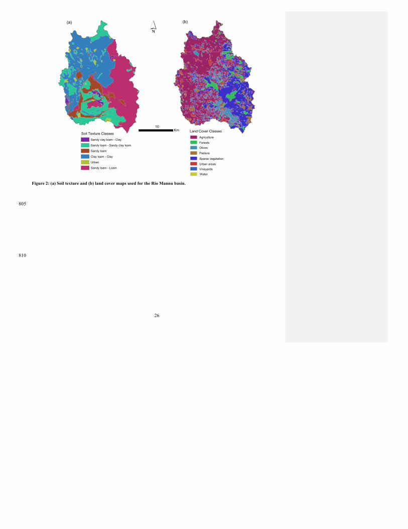
26

Figure 2: (a) Soil texture and (b) land cover maps used for the Rio Mannu basin.

805

810

´

Soil Texture Classes

Sandy clay loam - Clay

Sandy loam - Sandy clay loam

Sandy loam

Clay loam - Clay

Urban

Sandy loam - Loam

10

Km

.

Land Cover Classes

Agriculture

Forests

Olives

Pasture

Sparse vegetation

Urban areas

Vineyards

Water

(a) (b)

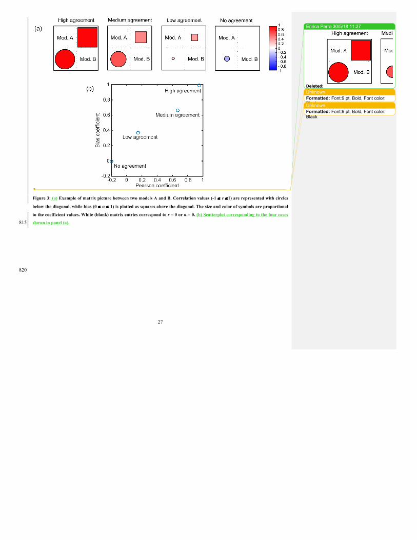
27

Figure 3: (a) Example of matrix picture between two models A and B. Correlation values (-1 ≤ r ≤1) are represented with circles

below the diagonal, while bias (0 ≤ α ≤ 1) is plotted as squares above the diagonal. The size and color of symbols are proportional

to the coefficient values. White (blank) matrix entries correspond to r = 0 or α = 0. (b) Scatterplot corresponding to the four cases

shown in panel (a). 815

820

Enrica Perra � 30/5/18 11:27

Deleted: 825 UnknownFormatted: Font:9 pt, Bold, Font color:BlackUnknownFormatted: Font:9 pt, Bold, Font color:Black

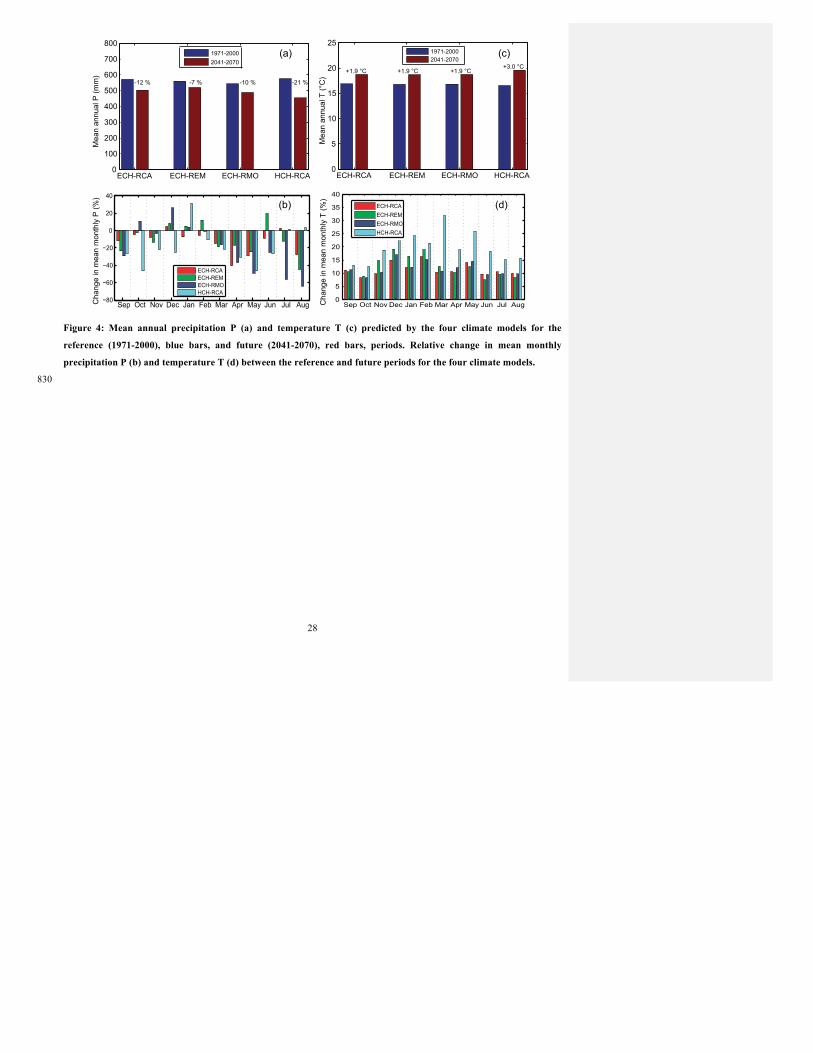
28

Figure 4: Mean annual precipitation P (a) and temperature T (c) predicted by the four climate models for the

reference (1971-2000), blue bars, and future (2041-2070), red bars, periods. Relative change in mean monthly

precipitation P (b) and temperature T (d) between the reference and future periods for the four climate models.

830

Cha

nge

in m

ean

mon

thly

P (%

)

Sep Oct Nov Dec Jan Feb Mar Apr May Jun Jul Aug−80

−60

−40

−20

0

20

40

ECH-RCAECH-REMECH-RMOHCH-RCA

Mea

n an

nual

T (°

C)

ECH-RCA ECH-REM ECH-RMO HCH-RCA0

5

10

15

20

25

1971-20002041-2070

+1.9 °C +1.9 °C +1.9 °C+3.0 °C

Mea

n an

nual

P (m

m)

ECH-RCA ECH-REM ECH-RMO HCH-RCA0

100

200

300

400

500

600

700

800

1971-20002041-2070

-12 % -7 % -10 % -21 %

Cha

nge

in m

ean

mon

thly

T (%

)

Sep Oct Nov Dec Jan Feb Mar Apr May Jun Jul Aug0

5

10

15

20

25

30

35

40

ECH-REMECH-RCA

ECH-RMOHCH-RCA

(a) (c)

(b) (d)

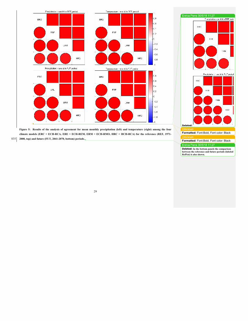
29

Figure 5: Results of the analysis of agreement for mean monthly precipitation (left) and temperature (right) among the four

climate models (ERC = ECH-RCA, ERE = ECH-REM, ERM = ECH-RMO, HRC = HCH-RCA) for the reference (REF, 1971-

2000, top) and future (FUT, 2041-2070, bottom) periods. 835

Enrica Perra � 30/5/18 11:27

Deleted:

UnknownFormatted: Font:Bold, Font color: BlackUnknownFormatted: Font:Bold, Font color: BlackEnrica Perra � 30/5/18 11:27Deleted: In the bottom panels the comparison between the reference and future periods (labeled RefFut) is also shown.

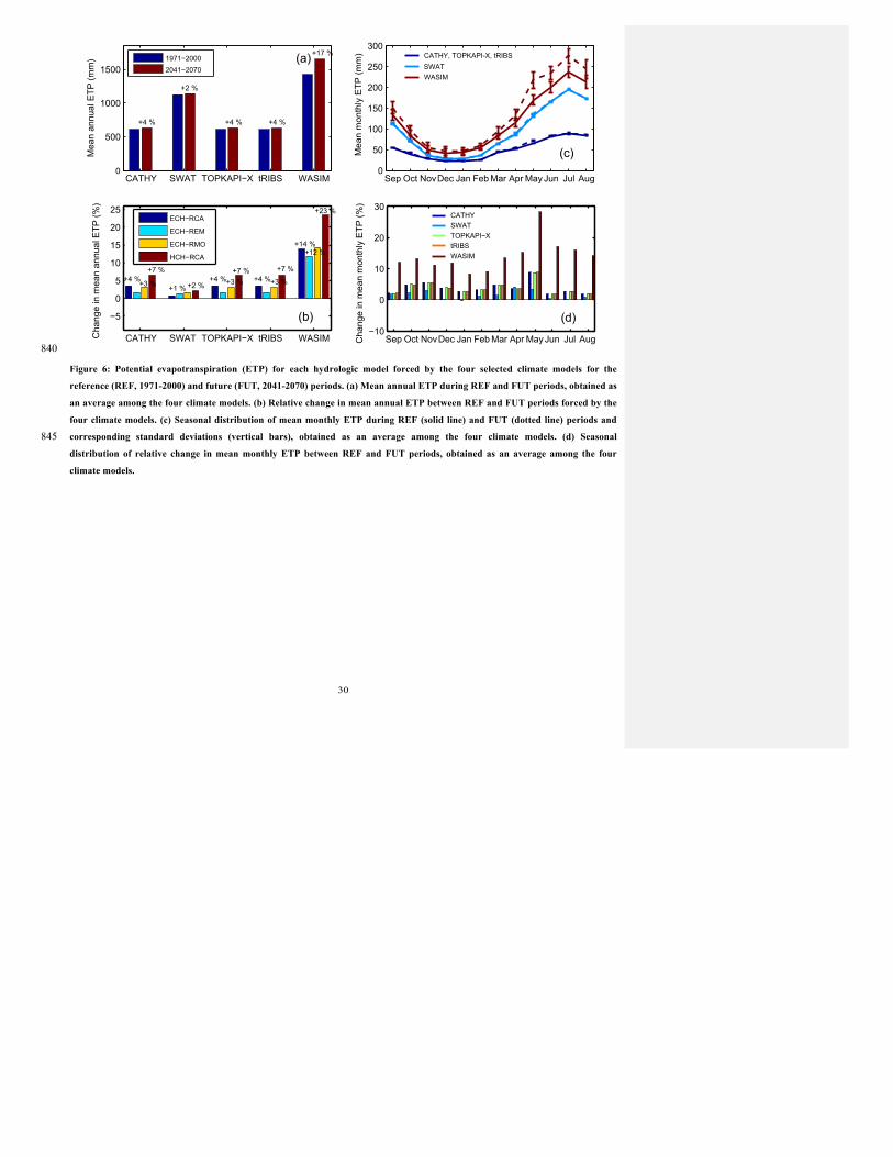
30

840

Figure 6: Potential evapotranspiration (ETP) for each hydrologic model forced by the four selected climate models for the

reference (REF, 1971-2000) and future (FUT, 2041-2070) periods. (a) Mean annual ETP during REF and FUT periods, obtained as

an average among the four climate models. (b) Relative change in mean annual ETP between REF and FUT periods forced by the

four climate models. (c) Seasonal distribution of mean monthly ETP during REF (solid line) and FUT (dotted line) periods and

corresponding standard deviations (vertical bars), obtained as an average among the four climate models. (d) Seasonal 845 distribution of relative change in mean monthly ETP between REF and FUT periods, obtained as an average among the four

climate models.

−5

0

5

10

15

20

25

Cha

nge

in m

ean

annu

al E

TP (%

) ECH−RCA

ECH−REM

ECH−RMO

HCH−RCA

CATHY SWAT TOPKAPI−X tRIBS WASIM0

500

1000

1500

Mea

n an

nual

ETP

(mm

)

1971−20002041−2070

(a)

(b)−10

0

10

20

30

Cha

nge

in m

ean

mon

thly

ETP

(%)

Sep Oct NovDec Jan Feb Mar Apr May Jun Jul Aug0

50

100

150

200

250

300

Mea

n m

onth

ly E

TP (m

m)

(d)

(c)

CATHYSWATTOPKAPI−XtRIBSWASIM

SWATCATHY, TOPKAPI-X, tRIBS

WASIM

+4 % +4 % +4 %

+2 %

+17 %

+4 %+7 %

+3 % +4 %+7 %

+3 %

+7 %

+3 %+4 %+2 %+1 %

+14 %

+23 %

+12 %

CATHY SWAT TOPKAPI−X tRIBS WASIM Sep Oct NovDec Jan Feb Mar Apr May Jun Jul Aug

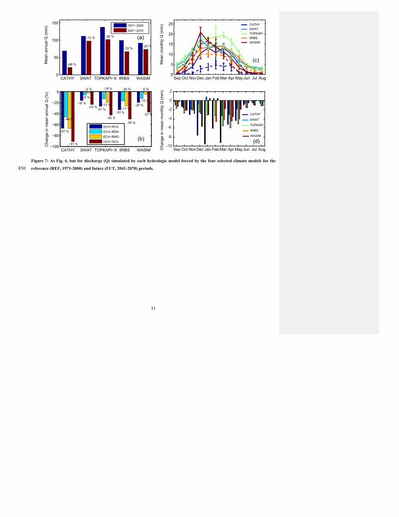
31

Figure 7: As Fig. 6, but for discharge (Q) simulated by each hydrologic model forced by the four selected climate models for the

reference (REF, 1971-2000) and future (FUT, 2041-2070) periods. 850


50

100

150

Mea

n an

nual

Q (m

m)

1971−20002041−2070

−100

−80

−60

−40

−20

0

Cha

nge

in m

ean

annu

al Q

(%)

ECH−RCAECH−REMECH−RMOHCH−RCA

-67 %

-46 %

-91 %

-16 %

-6 %

-2 %

-23 %-27 %

-13 %

-19 %

-42 %

-33 %-17 %

-26 %

-50 %

-20 %-12 %

-5 %

-37 %


5

10

15

20

25

Mea

n m

onth

ly Q

(mm

) CATHYSWATTOPKAPItRIBSWASIM

Cha

nge

in m

ean

mon

thly

Q (m

m)

-69 %

-12 % -26 %

-32 % -20 %

(a)

(c)

(b)-10

-8

-6

-4

-2

0

2

CATHY

SWAT

TOPKAPI

tRIBS

WASIM

(d)CATHY SWAT TOPKAPI−X tRIBS WASIM Sep Oct NovDec Jan Feb Mar Apr May Jun Jul Aug

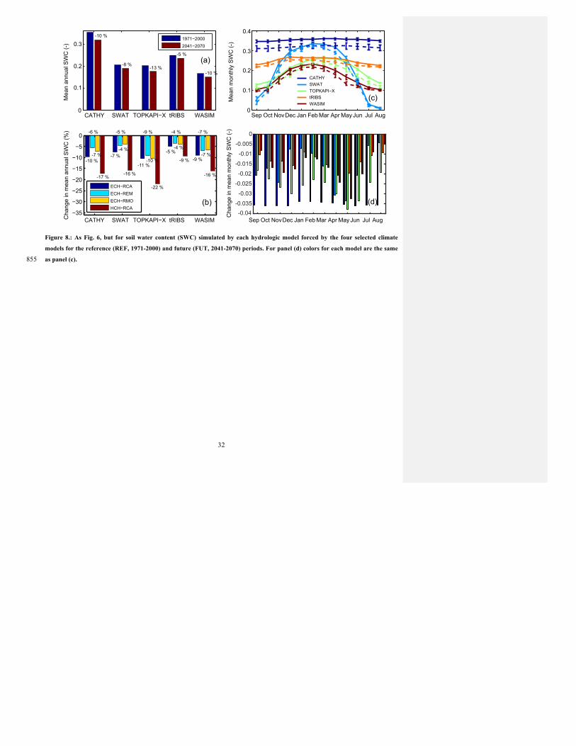
32

Figure 8.: As Fig. 6, but for soil water content (SWC) simulated by each hydrologic model forced by the four selected climate

models for the reference (REF, 1971-2000) and future (FUT, 2041-2070) periods. For panel (d) colors for each model are the same

as panel (c). 855


0.1

0.2

0.3

0.4

Mea

n m

onth

ly S

WC

(-)


Sep Oct NovDec Jan Feb Mar Apr May Jun Jul AugC

hang

e in

mea

n m

onth

ly S

WC

(-)


0.1

0.2

0.3

Mea

n an

nual

SW

C (-

)

1971−20002041−2070

−35

−30

−25

−20

−15

−10

−5

0

Cha

nge

in m

ean

annu

al S

WC

(%)


(a)

(c)

(b)

-10 %

-10 %

-8 %-13 %

-5 %

-10 %

-6 %

-7 %

-17 %

-7 %

-5 %

-4 %

-16 %

-11 %

-9 %

-10 %

-22 %

-5 %

-4 %

-4 %

-9 % -9 %

-7 %

-7 %

-16 %

-0.04-0.035

-0.03

-0.025

-0.02

-0.015

-0.01

-0.005

0

(d)

CATHY SWAT TOPKAPI−X tRIBS WASIM

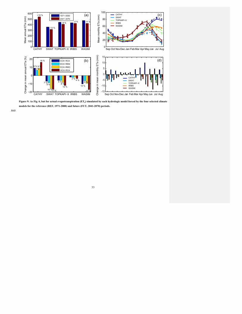
33

Figure 9: As Fig. 6, but for actual evapotranspiration (ETa) simulated by each hydrologic model forced by the four selected climate

models for the reference (REF, 1971-2000) and future (FUT, 2041-2070) periods.

860

CATHY SWAT TOPKAPI−X tRIBS WASIM−20

−10

0

10

20

Cha

nge

in m

ean

annu

al E

Ta (%

)



100

200

300

400

500

600

Mea

n an

nual

ETa

(mm

)

1971−20002041−2070


20

40

60

80

100

Mea

n m

onth

ly E

Ta (m

m) CATHY

SWATTOPKAPI−XtRIBSWASIM

Sep Oct NovDec Jan Feb Mar Apr May Jun Jul AugCha

nge

in m

ean

mon

thly

ETa

(mm

)

+10 %

-12 %

-8 % -2 % -11 %

9 %6 %

9 %

16 %

7 %9 %

16 %17 %

6 %8 %

12 %

2 %4 %

10 %

6 %

17 %

(a)

(b)

(c)

-15

-10

-5

0

5

10

15(d)


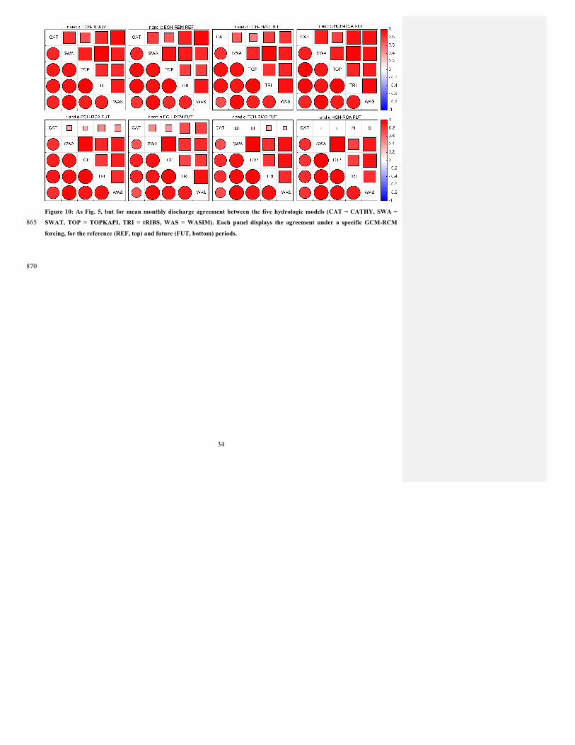
34

Figure 10: As Fig. 5, but for mean monthly discharge agreement between the five hydrologic models (CAT = CATHY, SWA =

SWAT, TOP = TOPKAPI, TRI = tRIBS, WAS = WASIM). Each panel displays the agreement under a specific GCM-RCM 865 forcing, for the reference (REF, top) and future (FUT, bottom) periods.

870

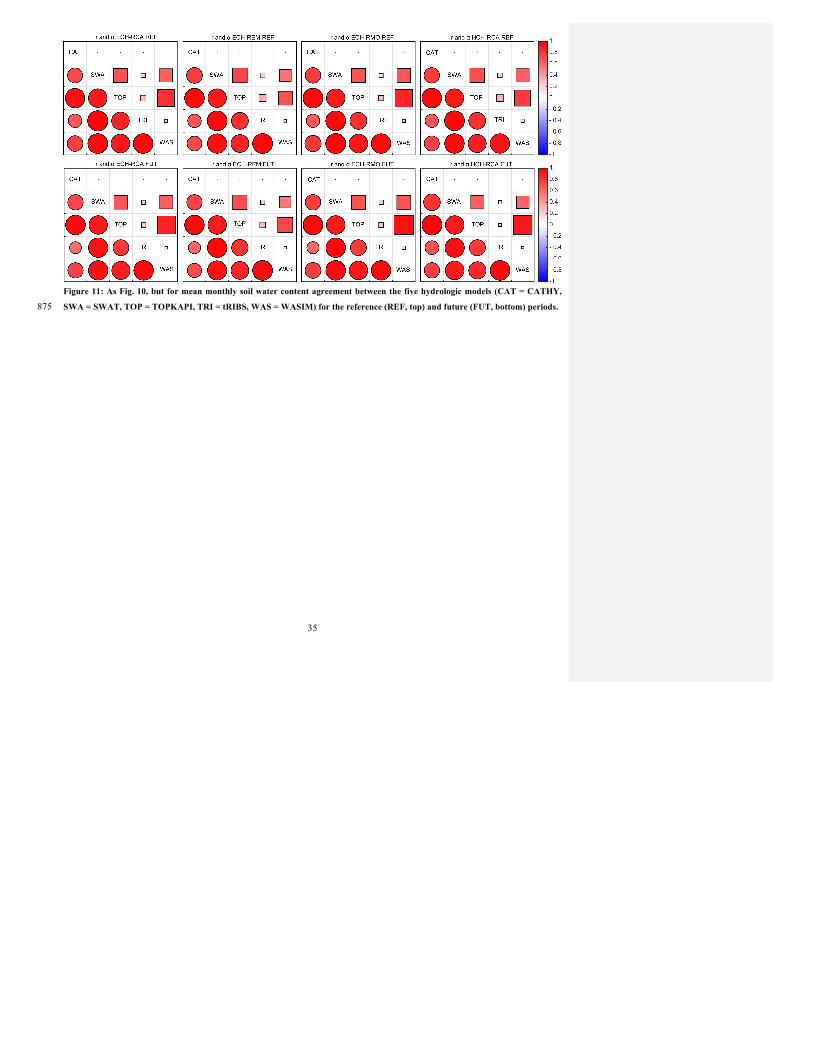
35

Figure 11: As Fig. 10, but for mean monthly soil water content agreement between the five hydrologic models (CAT = CATHY,

SWA = SWAT, TOP = TOPKAPI, TRI = tRIBS, WAS = WASIM) for the reference (REF, top) and future (FUT, bottom) periods. 875

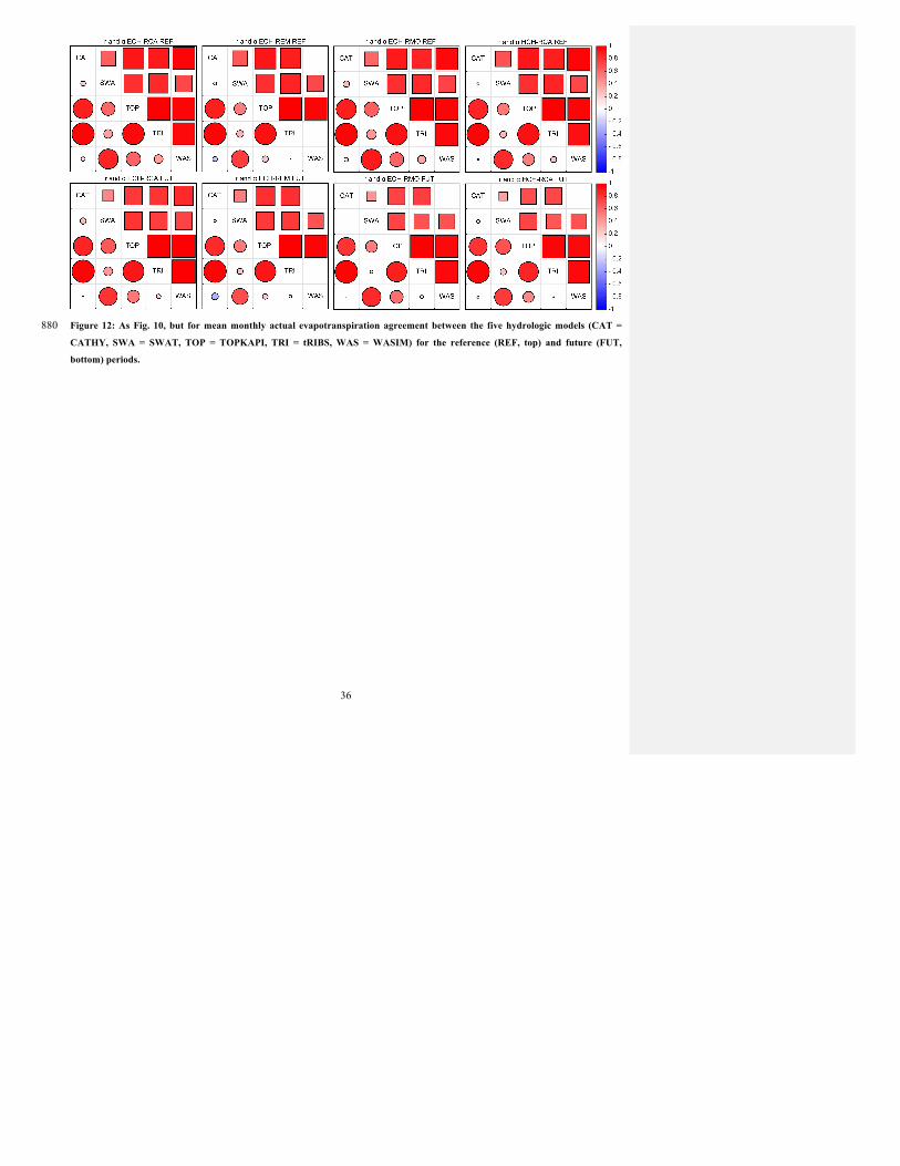
36

Figure 12: As Fig. 10, but for mean monthly actual evapotranspiration agreement between the five hydrologic models (CAT = 880 CATHY, SWA = SWAT, TOP = TOPKAPI, TRI = tRIBS, WAS = WASIM) for the reference (REF, top) and future (FUT,

bottom) periods.

hess-2018-165 Title of the manuscript: Multimodel assessment of ...

Documents