Hepp's bound for Feynman graphs and matroids - arXiv

Hepp’s bound for Feynman graphs andmatroids

Erik Panzer∗

October 29, 2019

We study a rational matroid invariant, obtained as the tropicalization ofthe Feynman period integral. It equals the volume of the polar of the matroidpolytope and we give efficient formulas for its computation. This invariantis proven to respect all known identities of Feynman integrals for graphs.We observe a strong correlation between the tropical and transcendentalintegrals, which yields a method to approximate unknown Feynman periods.

Contents1 Introduction 2

2 Definition and basic properties 82.1 Combinatorial definition . . . . . . . . . . . . . . . . . . . . . . . . . . . . 92.2 The Mellin integral . . . . . . . . . . . . . . . . . . . . . . . . . . . . . . . 102.3 Matroids . . . . . . . . . . . . . . . . . . . . . . . . . . . . . . . . . . . . . 122.4 Convergence . . . . . . . . . . . . . . . . . . . . . . . . . . . . . . . . . . . 142.5 Zeroes and shuffles . . . . . . . . . . . . . . . . . . . . . . . . . . . . . . . 152.6 Poles and factorizations . . . . . . . . . . . . . . . . . . . . . . . . . . . . 182.7 Other matroid invariants . . . . . . . . . . . . . . . . . . . . . . . . . . . . 21

3 Flag formulas 233.1 Bridges and ears . . . . . . . . . . . . . . . . . . . . . . . . . . . . . . . . 233.2 Flats and cuts . . . . . . . . . . . . . . . . . . . . . . . . . . . . . . . . . . 283.3 Cyclic flats . . . . . . . . . . . . . . . . . . . . . . . . . . . . . . . . . . . 32

4 Symmetries 344.1 Duality . . . . . . . . . . . . . . . . . . . . . . . . . . . . . . . . . . . . . 364.2 Products and 2-sums . . . . . . . . . . . . . . . . . . . . . . . . . . . . . . 37

∗All Souls College, University of Oxford, UK, [email protected]

1

arX

iv:1

908.

0982

0v2

[m

ath-

ph]

28

Oct

201

9

4.3 Completion . . . . . . . . . . . . . . . . . . . . . . . . . . . . . . . . . . . 404.4 Twist . . . . . . . . . . . . . . . . . . . . . . . . . . . . . . . . . . . . . . 454.5 Fourier split and uniqueness . . . . . . . . . . . . . . . . . . . . . . . . . . 48

5 φ4 theory 515.1 Period correlation . . . . . . . . . . . . . . . . . . . . . . . . . . . . . . . . 515.2 Unexplained identities . . . . . . . . . . . . . . . . . . . . . . . . . . . . . 535.3 Improved bounds . . . . . . . . . . . . . . . . . . . . . . . . . . . . . . . . 55

6 Polyhedral geometry 596.1 Singularities, facets and vertices . . . . . . . . . . . . . . . . . . . . . . . . 626.2 Factorization . . . . . . . . . . . . . . . . . . . . . . . . . . . . . . . . . . 636.3 Computations . . . . . . . . . . . . . . . . . . . . . . . . . . . . . . . . . . 646.4 Shape . . . . . . . . . . . . . . . . . . . . . . . . . . . . . . . . . . . . . . 656.5 Tree decomposition . . . . . . . . . . . . . . . . . . . . . . . . . . . . . . . 666.6 Period correlation . . . . . . . . . . . . . . . . . . . . . . . . . . . . . . . . 67

7 Outlook 68

References 69

1 IntroductionTo a connected graph G with N edges, Kirchhoff [76] attached the graph polynomial

ΨG =∑T∈TG

∏e/∈T

xe ∈ Z[x1, . . . , xN ] (1.1)

given by a sum over the set TG of spanning trees. In the context [12, 87] of perturbativequantum field theory, the variables xe associated to each edge e are called Schwingerparameters. The scalar Feynman integral encoded by G contributes the period [9, 80]

P (G) =(N−1∏e=1

∫ ∞0

dxe

)1

Ψd/2G

∣∣∣∣∣xN=1

(1.2)

to the beta function of the field theory in d dimensions of space-time [79, 97, 107].This integral is well-defined when G is primitive logarithmically divergent (p-log), whichmeans that ω(G) = 0 and ω(γ) > 0 for every non-empty, proper subgraph γ ⊂ G, where

ω(G) = |G| − d2 · `(G) = # edges in G − d

2 ·# loops in G

is called the superficial degree of convergence of G. For example, the complete graph K4with |K4| = 6 edges and `(K4) = 3 loops is p-log in d = 4 dimensions. Its period is

P (K4) = P( )

= 6ζ (3) ≈ 7.21 (1.3)

2

delete v←−−−−−w

v

delete w−−−−−→

Figure 1: Two non-isomorphic graphs with the same completion.

in terms of the Riemann zeta function. The transcendental numbers [22, 26, 90] emergingas periods of graphs are extremely difficult to compute exactly, and even approximationsare very challenging. For most graphs, the periods thus remain unknown.

This complexity stimulates the search for simpler graph invariants, that are easier tocompute, but still capture information about the period [43]. To be meaningful, suchinvariants should obey period identities. For example, conformal invariance [21] equatesthe periods of the complements G\v and G\w in Figure 1. This completion relation andthe product identity show that

P( )

= P( )

= P( )2

= 36ζ(3)2.

Further relations include planar duality, the twist [97] and the recently discovered Fouriersplit [70], which generalizes the uniqueness relations [73]. It is a challenge to constructnon-trivial graph invariants with these symmetries. In fact, apart from the period itself,only two such invariants had been found so far: the c2 invariant [98] and the (extended)graph permanent [44, 45].The c2 invariant is constructed from the point counts of the hypersurface ΨG = 0 ⊂

FNq over finite fields Fq. It is related to the number theory of the period [26, 27, 29, 90],but several of the symmetries remain conjectural despite recent progress [54, 55, 118].For the permanent (of copies of the incidence matrix), the first four symmetries aboveare proven. It is not yet clear, however, what the permanent implies for the period.

In this paper, we study a new invariant obtained by a drastic simplification of theperiod integral: In the spirit of tropical geometry, replace ΨG by its maximal monomial,

ΨtrG := max

T∈TG

∏e/∈T

xe. (1.4)

This function is locally just some monomial, but which particular monomial it is dependson the actual values of the Schwinger parameters. We refer to the corresponding integral

H(G) :=(N−1∏e=1

∫ ∞0

dxe

)1

(ΨtrG)d/2

∣∣∣∣∣xN=1

∈ Q (1.5)

as the Hepp bound, which defines a rational number for each p-log graph. It is indeed abound on the period, since we have Ψtr

G ≤ ΨG ≤ ΨtrG · |TG| and therefore

H(G) · |TG|−d/2 ≤ P (G) ≤ H(G) . (1.6)

3

Hepp [69] used this idea to deduce the convergence of the integral P (G) from a power-counting argument, by dissecting the integration domain into regions

Dσ =xσ(1) < · · · < xσ(N)

⊂ RN

+ (1.7)

according to the permutation σ of the edges determined by the order of the Schwingerparameters. These regions Dσ, called Hepp sectors, have wide applications to renormal-ization, regularization and asymptotic expansion of Feynman integrals [7, 48, 101, 103].

Symmetries The surprising observation is that the crude bound (1.5) is in fact verywell behaved and closely related to the actual period (1.2). Firstly, we will prove

Theorem 1.1. The Hepp bound respects the five period symmetries from [70, 97].

This suggests that graphs with equal periods might also have the same Hepp bound.Analogous conjectures were made for the c2 invariant and the permanent mentionedabove. We conjecture that, for the Hepp bound, also the converse is true—at least inthe case of φ4 theory [77]. Concretely, we say that a graph G is in φ4 if it is p-log ind = 4 dimensions and every vertex has degree at most 4 (for example K4 from before).More than a thousand φ4 periods are known [90], and they are all in agreement with:

Conjecture 1.2. Two φ4 graphs have equal periods if and only if they have equal Heppbounds.

This significant strengthening of Theorem 1.1 is wrong for the c2 invariant and the per-manent, because there exist pairs of φ4 graphs with the same c2 invariant or permanent,but whose periods are known and different. There still seems to be a possibility, however,that c2 and the permanent combined might distinguish periods [44, Appendix A].The “faithfulness” of the Hepp bound according to Conjecture 1.2 would imply new

relations between yet unknown periods, which are not explained by the five operationsdiscussed in [70, 97]. The first examples of still unproven, conjectural identities of φ4

periods appear at 8 loops, where in the notation of [97] we find two pairs

H(P8,30\v) = H(P8,36\v) = 17244883 and H(P8,31\v) = H(P8,35\v) = 536760 (1.8)

of graphs with equal Hepp bounds and thus conjecturally equal periods (see Figure 24).Of these four, only P (P8,31) ≈ 460.09 could be computed exactly in [97]. The combina-torial origin of the equalities (1.8) is currently not understood.

Hepp–Period correlation For explicit computations of the Hepp bound, the integralrepresentation (1.5) is not very practical. In Proposition 3.2 we rewrite it as a sum overflags of bridgeless subgraphs, a generalization of ear decompositions. This formula reads

H(G) =∑

γ1(···(γ`=G

|γ1| · |γ2 \ γ1| · · · |G \ γ`−1|ω(γ1) · · ·ω(γ`−1)

4

1.5

2.5

3.5

4.5

8 10 12 14 16 18

H(G)/104

P(G)/102b

bb

bb

b

bb

b

bb

b

P7,8

P7,11

P7,9

P7,5 = P7,10

P7,6

P7,4 = P7,7

P7,3

P 33,1

P7,2

P3,1 · P5,1

P 24,1

P7,1

Figure 2: The period as a function of the Hepp bound for all φ4 periods at 7 loops, thedashed line is a power law fit P (G) ≈ 3.96/105 · [H(G)]1.3495. The graphs arelabelled according to [97], see Table 2 for details.

and allows the calculation of H(G) for most graphs of interest. We used it to obtain theHepp bounds of all φ4 graphs with `(G) ≤ 11 loops. For example, we find

H(K4) = H( )

= 84, (1.9)

which should be compared with the much smaller period (1.3). So the Hepp bound is verycrude indeed and it can exceed the period by several orders of magnitude. Surprisingly,this bound nonetheless allows us to predict the numeric values of periods within a rangeof a few percent. Namely, we observe that the period is very strongly correlated withthe Hepp bound, as illustrated in Figure 2. At higher loop orders, a smooth curveinterpolating the known periods then gives estimates for unknown periods.It is remarkable that the rational number H(G), which is easy to compute for any

graph, gives such a sensitive measure of the intricate period integral P (G). This con-nection was exploited in [79] to estimate the contributions from higher orders in pertur-bation theory to a calculation of the beta function in φ4 theory, and we are optimisticthat generalizations and refinements of this method can provide a new approach to thenumeric evaluation of Feynman integrals, efficient even at large loop orders.

Geometry The correlation of H(G) with P (G) is so far an empirical observation, butit appears to be related to a geometric interpretation of the Hepp bound. The approxi-mation of Feynman integrals by the method of sector decomposition uses a resolution ofsingularities [11] of the graph hypersurface ΨG = 0. This is achieved most efficientlyby a triangulation of the normal fan of the Newton polytope of ΨG [18, 72, 95, 101]. Itis also known as the spanning tree polytope of G, and we define it as the convex hull

NG := conv ~vT : T ∈ TG ⊂ RN (1.10)

of the characteristic vectors ~vT of the spanning trees T , with coordinates ~vT,e = 1 for alledges e ∈ T in the tree, and ~vT,e = −1 whenever e /∈ T . The polar of this polytope is

N G =⋂

T∈TG

~y : ~y ·~vT ≤ 1 ⊂ RN . (1.11)

5

Theorem 1.3. For a graph G with N edges that is p-log in d = 4 dimensions, we have

H(G) = (N − 1)! ·Vol (N G ∩ yN = 0) . (1.12)

The asymptotic growth of period integrals implies that the volume of the polytope N Gis concentrated on directions near the facet normals ~vT , like a cross-polytope. Dually,NG behaves like a cube in the sense that its volume is concentrated in the corners.We show in Lemma 6.23 that the period integral (1.2) can be written as an integralof a log-concave function over the polytope N G, and argue that this explains at leastqualitatively the correlation between the period and H(G).

An important tool for our proofs of the symmetries is a functional generalization ofthe Hepp bound: Instead of the mere number (1.5), we consider the rational function

H(G,~a) :=(N−1∏e=1

∫ ∞0

xae−1e dxe

)1

(ΨtrG)d/2

∣∣∣∣∣xN=1

∈ Q(a1, . . . , aN ) (1.13)

given by the Mellin transform of (ΨtrG)−d/2. This is a well-defined rational function for

arbitrary biconnected graphs, and not just p-log graphs. The period symmetries from[70, 97] extend to this functional setting, and we prove them in this generality. We exploitthat H(G,~a) is a function with simple poles, located on hyperplanes ~a : ω(γ) = 0 forsuitable graphs γ ⊂ G, where the superficial degree of convergence is the linear function

ω(γ) =∑e∈γ

ae −d

2 · `(γ).

The Hepp bound has a pole at ω(γ) = 0 precisely when γ and its quotient G/γ arebiconnected. Such subgraphs correspond to a facet of the Newton polytope, and itfactorizes as Nγ×NG/γ ⊂ ∂NG. Generalizing (1.12), the function H(G,~a) is the volumeof the polar of the translated Newton polytope ~a + NG, such that the facets of NGcorrespond directly to the poles of the Hepp bound. Hence the residues are products

Resω(γ)=0

H(G,~a) = H(γ,~a′

)· H(G/γ,~a′′

)(1.14)

and separate the dependence on variables ~a′ = (ae)e∈γ associated to the subgraph andthe quotient, ~a′′ = (ae)e∈G\γ . This gives a tool for inductive proofs of identities ofrational functions, similar to the BCFW recursion [19].The same mechanism of associating rational functions with simple poles and factoriz-

ing residues to polytopes is also used for tree level scattering amplitudes, under the namecanonical forms [3]. In that context, the Mellin variables ae play the role of Mandelstaminvariants obtained from momenta of particles; the factorization above is interpreted asunitarity, and the fact that only simple poles occur is attributed to locality.

Matroid invariants The Hepp bound (1.13) is not restricted to graphs and extends toall matroids. In this paper we work in this more general universe, with the sole exceptionof three symmetries: completion, twist and Fourier-split are only defined for graphs.

6

Our definition of the Hepp bound gives zero whenever a matroid is not connected.Otherwise, let SM denote the set of submatroids γ (M such that both γ and M/γ areconnected. These γ label the facets of NM , and we will show:

Proposition 1.4. The Hepp bound H(M,~a) of a connected matroid M is a non-zerorational function with simple poles, precisely on the hypersurfaces ω(γ) = 0 for γ ∈ SM ,and factorizing residues as in (1.14).

Matroid polytopes have been studied extensively, but little seems to be known abouttheir polars. Our findings suggest that the volume of the (sliding) polar N M (~a), as arational function, is a very interesting matroid invariant. It has a rich structure and itdetermines the matroid completely (Remark 2.3). Furthermore, the symmetries of theHepp bound show that polar volumes are subject to more identities than the volumes ofthe matroid polytopes themselves.

Outline of the paperThis article aims to be broadly accessible and includes relevant definitions and resultsfrom the combinatorial literature. The focus here is on the mathematical properties ofthe Hepp bound, but the particle physicist will recognize the motivation and applications.We give a combinatorial definition of the Hepp bound for arbitrary matroids in sec-

tion 2, which is consistent with the Mellin integral, and obtain its poles and the factor-ization of residues discussed above. We compute the Hepp bound of uniform matroids,and illustrate relations to Crapo’s and Derksen’s matroid invariants in subsection 2.7.The remaining sections are essentially independent of each other: Formulas in terms of

flags of bridgeless submatroids or flats are derived in section 3 and applied to computethe Hepp bound of all wheel graphs. The five period symmetries are proven for theHepp bound in section 4. We report the results for φ4 graphs in section 5, addressingthe correlation with the period and unexplained identities, and we discuss improvementsof the Hepp bound. The convex geometric point of view is worked out in section 6.

AcknowledgmentsI am indebted to Karen Yeats for invitations to SFU Vancouver in early 2016, wherethe groundwork for this research was laid, and to the University of Waterloo in 2018.At these workshops I benefited also from long discussions with Michael Borinsky, IainCrump, Alejandro Morales and Yoav Len. Furthermore I thank the organizers and theparticipants of Structures in local quantum field theory in Les Houches and Amplitudesat SLAC for chances to present aspects of this work in 2018.This project and my understanding was further shaped by inputs from Francis Brown,

Johannes Schlenk, Carlos Mafra, Oliver Schnetz, David Broadhurst, Konrad Schultka,Jacob Bourjaily, Matteo Parisi and Giulio Salvatori.Finally I thank ITS at ETH Zürich for hospitality and perfect working conditions dur-

ing final stages of the preparation of this manuscript in 2019, at the thematic programmeModular forms, periods and scattering amplitudes.

7

2 Definition and basic propertiesOur construction is motivated by the Feynman integrals of perturbative quantum fieldtheory [23, 87, 104]. The period P (G) defined in (1.2) is only one particular integralthat can be associated to a graph G. More generally, one considers the Mellin transform

P (G,~a) :=(N−1∏e=1

∫ ∞0

xae−1e dxe

)1

Ψd/2G

∣∣∣∣∣xN=1

(2.1)

of Ψ−d/2G as a multivariate function of the variables ~a = (a1, . . . , aN ), which we callindices. In particle physics, they are the exponents of the momentum space propaga-tors attached to each edge of the graph. Studying the dependence of (2.1) on ~a hasproven exceptionally fruitful to understand Feynman integrals. For example, differenceequations with respect to the indices are heavily used in practical calculations [33, 66].The function (2.1) is called the analytically regularized Feynman integral. If the graph

G is biconnected, this integral converges for suitable indices, and it extends to a uniquemeromorphic function of the indices, with poles on families of hyperplanes [104].

Example 2.1. The cycle C2 = with two edges (also called “bubble”) has `(C2) = 1loop and it is p-log when a1, a2 > 0 and d

2 = a1 + a2. Since C2 has precisely twospanning trees e1 and e2, consisting of the individual edges, the graph polynomialis ΨC2 = x1 + x2. The regularized Feynman integral therefore becomes

P(

,~a)

=∫ ∞

0

xa1−11 dx1

(x1 + 1)a1+a2= Γ(a1)Γ(a2)

Γ(a1 + a2) ,

which is meromorphic in ~a ∈ C2 with poles on the hyperplanes a1, a2 ∈ Z≤0.

The Hepp bound (1.13) is the variant of (2.1) obtained by replacing the graph poly-nomial ΨG with its tropical analogue Ψtr

G. This yields a rational function of the indices,which captures precisely the first pole in each family of singularities of P (G,~a).

Example 2.2. The tropical graph polynomial of the bubble is ΨtrC2

= max x1, x2.Whenever both indices are positive, a1 > 0 and a2 > 0, the Hepp bound integral

H(

,~a)

=∫ ∞

0

xa1−11 dx1

(max x1, 1)a1+a2=∫ 1

0xa1−1

1 dx1 +∫ ∞

1x−a2−1

1 dx1 = a1 + a2a1a2

is absolutely convergent. It has poles at a1 = 0 and a2 = 0, and it can be obtainedformally by replacing each gamma function in P (C2,~a) by its first pole, Γ(s) 7→ 1/s.

The inequality ΨtrG ≤ ΨG ≤ Ψtr

G · |TG| underlying (1.6) shows that both Mellin integrals(1.13) and (2.1) have the same domain of convergence. Outside this domain, the integralsdefine the Hepp bound and Feynman integral only indirectly via analytic continuation.Our first goal is a definition of the Hepp bound as an explicit rational function, valid forall indices, and without reference to integrals.

8

Remark 2.3. If G is biconnected with N ≥ 2 edges, we will see that the Mellin integralsconverge for suitable indices. The inverse Mellin transform (an integral over ~a) thenallows us to recover the function ~x 7→ Ψtr

G(~x) from the Hepp bound H(G,~a). Everyspanning tree dictates Ψtr

G in some domain of the Schwinger parameters, so we canobtain the set TG from the tropical graph polynomial. Similarly, we can reverse engineerthe spanning trees from the Feynman integral P (G,~a). This may be illustrated as

H(G,~a)←→ ΨtrG(~x)←→ TG ←→ ΨG(~x)←→ P (G,~a) ,

where each arrow A←→ B indicates that A determines B and vice versa. We see thatthe rational function H(G,~a) completely determines the Feynman integral P (G,~a) as afunction of ~a. This does not, however, impinge on Conjecture 1.2, which is a statementabout special values at a1 = · · · = aN = 1.

2.1 Combinatorial definitionWe consider arbitrary undirected graphs, which may have multiple edges between thesame pair of vertices, and edges with both endpoints at the same vertex (self-loops) arealso allowed. We write |G| := |EG| for the number of edges, which is often also denotedby N . The loop number `(G) is the first Betti number of the graph, which is

`(G) = |G| − |VG|+ κ(G) (2.2)

in terms of the number |VG| of vertices and the number κ(G) of connected components.The superficial degree of convergence of a subgraph γ ⊆ G is the linear function

ω(γ) = ω~a(γ) :=∑e∈γ

ae −d

2 · `(γ), (2.3)

and we will always impose the condition ω(G) = 0 called ‘logarithmic divergence’. Forgraphs with loops, it means that the dimension is determined by the indices as

d = 2a1 + · · ·+ aN`(G) .

For forests (graphs without loops), the dimension disappears from (2.3) and plays norole. The condition ω(G) = 0 then imposes the constraint a1 + · · ·+ aN = 0.

Definition 2.4. If G is a graph with N ≥ 1 edges and we are given a permutation σof its edges, we denote by Gσk := σ(1), . . . , σ(k) the subgraphs formed by the first kedges in the order σ. The Hepp bound of G is the homogeneous rational function

H(G,~a) :=∑σ∈SN

1ω(Gσ1 ) · · ·ω(GσN−1) (2.4)

of degree 1−N , obtained by summing over all N ! permutations. For a single edge N = 1,the empty product in the denominator is defined as unity such that H(G, a1) = 1.

9

C6 C5 C4 C3 C2 = D2 D3 D4 D5 D6

Figure 3: The first few cycle/polygon graphs Cn, and the bonds/dipoles/melons Dn.

Example 2.5. For the bubble from Example 2.2, there are only two N ! = 2 permuta-tions to consider. The graphs G(1,2)

1 = 1 and G(2,1)1 = 2 formed by the first edges

have no loops and we recover the result H(C2,~a) = 1a1

+ 1a2

from ω(e) = ae.

Example 2.6. Consider any cycle CN (Figure 3) with unit indices a1 = · · · = aN = 1.Because every proper subgraph is a forest, we get ω(Gσk) = k in (2.4). So each of the N !summands contributes 1/(N − 1)! and the total Hepp bound is H(CN ) = N = d/2.

Example 2.7. If G = consists of two isolated edges, we obtain the same expression1a1

+ 1a2

from the sum (2.4). But in this case without loops, we consider it as a functionon the hyperplane 0 = ω(G) = a1 + a2 where it vanishes. Hence we find H( ,~a) = 0.

In the same way, we will see later that H(G,~a) = 0 for all forests with N ≥ 2 edges.The Hepp bound is therefore only really interesting for graphs with loops.

2.2 The Mellin integralIn order to relate Definition 2.4 to the integral (1.13) for arbitrary graphs, we define thetropical graph polynomial Ψtr

G for disconnected graphs similarly as in (1.4), but with asum over all spanning forests. In particular, Ψtr

G = 1 whenever G is itself a forest.It follows from (2.2) that the graph polynomial is homogeneous of degree `(G), so

ΨtrG(λx1, . . . , λxN ) = λ`(G) ·Ψtr

G

for all positive λ > 0 and ~x ∈ RN+ . The function (Ψtr

G)−d/2∏e x

aee is therefore homoge-

neous of degree ω(G), and the condition ω(G) = 0 ensures that the Mellin integral (1.13)is in fact an integral over projective space, written in the chart xN = 1. It is thereforeirrelevant which edge we choose to label N , and we can write (1.13) symmetrically as

H(G,~a) =∫PG

Ω(~a)(Ψtr

G)d/2.

The integration domain is the positive orthantPG := [x1 : · · · : xN ] : x1, . . . , xN > 0 ⊂RPN−1 inside real projective space, and Ω(~a) denotes the N − 1 form

Ω(~a) :=(

N∏e=1

xae−1e

)N∑e=1

(−1)e−1xe∧f 6=e

dxf . (2.5)

10

To compute the integral, we subdivide the domain PG into the Hepp sectors (1.7):

H(G,~a) =∑σ∈SN

∫Dσ

Ω(~a)(Ψtr

G)d/2.

Each summand is an integral over the projective simplex with 0 < xσ(1) < · · · < xσ(N).Hepp noted that within every sector Dσ, there is a unique spanning tree Tσ ∈ TG thatdominates all others, i.e. the function Ψtr

G is given by a fixed monomial inside the sector:

ΨtrG(x)

∣∣∣x∈Dσ

=∏e/∈Tσ

xe. (∗)

Indeed, the dominating spanning tree Tσ (or forest, if G is disconnected) is nothing butthe minimum weight spanning tree with respect to the edge weights log xe, and followingKruskal [82] this spanning tree is uniquely determined by the total order σ of the weights:

Lemma 2.8 (Kruskal’s greedy algorithm). If we are given a total order of the edgeweights, hence a permutation σ ∈ SN of the edges, then the minimum weight spanningforest Tσ consists of precisely those edges that do not increase the loop number:

Tσ =σ(k) : `(Gσk) = `(Gσk−1)

∈ TG.

The edges e /∈ Tσ contributing to the dominating monomial (∗) are therefore preciselythose edges e = σ(k) at which the loop number `(Gσk) = 1 + `(Gσk−1) increases. In theaffine chart xσ(N) = 1, the integral over a Hepp sector can therefore be written as

∫Dσ

Ω(~a)(Ψtr

G)d/2=∫

0<xσ(1)<···<xσ(N)=1

N−1∏k=1

xaσ(k)−1− d2

(`(Gσk )−`(Gσk−1)

)σ(k) dxσ(k).

Changing variables to yk = xσ(k)/xσ(k+1), this evaluates to the summand in (2.4):

N−1∏e=1

∫ 1

0y

(∑k

i=1 aσ(i))−1− d2 `(G

σk )

k dyk = 1ω(Gσ1 )· · ·ω(GσN−1) .

This integral converges precisely when all real parts Reω(Gσ1 ), . . . ,Reω(GσN−1) > 0 arepositive. We can summarize this calculation as follows:

Proposition 2.9. The Mellin integrals (1.13) and (2.1) converge precisely for thoseindices ~a ⊂ CN whose real part lies in the open convex polyhedral cone

Θ :=⋂

∅6=γ(G

~a ∈ RN : ω~a(γ) > 0

⊆ RN . (2.6)

For such ~a, the Hepp bound integral (1.13) coincides with the function in Definition 2.4.

11

The characterization of the convergence of Feynman integrals in terms of power count-ing conditions ω(γ) > 0 is fundamental for renormalization in physics [57, 115]. Manyof these constraints are redundant, however. The independent constraints are given in(2.20); for more general Feynman integrals with kinematics see [104, 105].In the sequel we will mostly use the combinatorial formula (2.4), which allows us to

ignore questions of convergence. However, the convergence domain Θ is non-empty inall cases of interest (Lemma 2.16), and we may thus use the Mellin integral freely.

Example 2.10. We compute the Hepp bound of the cycle graph CN as a function ofthe indices. Its N spanning trees are the edge complements T = CN \ e and thusΨtr = max x1, . . . , xN. The integral over the domain where Ψtr = xk is maximal gives

∫Ψtr=xk

Ω(~a)(Ψtr)d/2

=

∏e 6=k

∫ xk

0xae−1e dxe

xak−1k

xd/2k

∣∣∣∣xk=1

=∏e 6=k

1ae,

computed in the chart xk = 1. Adding all these contributions, we find in generalizationof Example 2.2 and Example 2.6 that the full Hepp bound function is given by

H(CN ,~a) = a1 + · · ·+ aNa1 · · · aN

= d/2a1 · · · aN

. (2.7)

2.3 MatroidsThe Hepp bound depends only on the set of spanning trees, so it is not sensitive to thefull combinatorial structure of a graph. This suggests a generalization, and indeed theweaker notion of a matroid is sufficient. We use standard terminology as in [88].A matroid M = (EM , IM ) consists of a ground set EM and a non-empty family IM

of subsets of EM , called the independent sets, such that

1. Every subset δ ⊂ γ of an independent set γ ∈ IM is independent: δ ∈ IM .

2. If δ, γ ∈ IM are independent and |δ| < |γ|, then we can find an element e ∈ γ \ δsuch that δ ∪ e ∈ IM is independent.

Example 2.11. Every graph defines the cycle matroid M(G) = (EG, IG) on the edgesEG as ground set [88, 111]. Its independent sets IG = γ ⊆ EG : `(γ) = 0 are the forests(loopless subgraphs) of G. It is well understood when two graphs share isomorphic cyclematroids [108, 117], and this is exploited in practical calculations [114].

Matroids that come from graphs in this way are called graphic, and most matroids arenot graphic. Even non-graphic matroids do arise in Feynman integral calculations [81].

Example 2.12. The uniform matroid U rn with rank 0 ≤ r ≤ n is defined on the groundset 1, . . . , n and its independent subsets are precisely all subsets of size at most r.The extremes Unn and U0

n are the cycle matroids of forests and collections of self-loops,respectively. The only other graphic uniform matroids are the cycles Un−1

n∼= M(Cn)

and the bonds (also called dipoles) U1n∼=M(Dn) illustrated in Figure 3.

12

The maximal independent sets BM ⊆ IM of a matroid are called its bases, and inthe case of the cycle matroid the bases are precisely the spanning trees. The (tropical)graph polynomial therefore generalizes naturally to the (tropical) matroid polynomial1

ΨM :=∑T∈BM

∏e/∈T

xe and ΨtrM := max

T∈BM

∏e/∈T

xe, (2.8)

and the Mellin integral (1.13) may thus be considered for an arbitrary matroid. We canalso extend the combinatorial Definition 2.4 to all matroids: The rank of a submatroidγ ⊆ EM is the maximal size of an independent set contained in it,

rk(γ) = maxF∈IM ,F⊆γ

|F | .

The surplus of edges is the corank `(γ) := |Eγ | − rk(γ), and in the case of a graphicmatroid it is precisely the loop number (2.2). Using the corank, the superficial degree ofconvergence (2.3) defines a linear function ω(γ) for each submatroid, and so (2.4) definesthe Hepp bound for all matroids.Example 2.13. The uniform matroid M = U rn with rank 0 < r < n has ` = n − rloops, such that d

2 = n` for unit indices a1 = · · · = an = 1. Every subset γ ⊂ U rn with

k = |γ| ≤ r elements has rank k, and for k > r, the rank of γ is r. Every permutationof the edges therefore produces the same sequence of superficial degrees of convergence,

ω(Mσk ) =

k for 1 ≤ k ≤ r andk − (k − r)n` = (n− k) r` for r < k < n.

Therefore the Hepp bound of the uniform matroid with unit indices is given by

H(U rn) = n!(r − 1)!`!

(`

r

)`. (2.9)

This reproduces the cycles H(Cn) = H(Un−1n

)= n from Example 2.6. For the smallest

non-graphic matroid we get H(U2

4)

= 12.Remark 2.14. The uniform matroid is the unique minimizer of the Hepp bound among allmatroids of fixed rank and size: If M has n elements and rank r, then H(M) ≥ H(U rn),with equality if and only if M ∼= U rn. This follows from BM ⊆ BUrn and (2.8).

Almost all results in this paper apply to arbitrary matroids; in fact, the only exceptionare the completion and twist symmetries in section 4, which we only define for graphs.In particular, the compatibility of the Mellin integral and the combinatorial definitionas stated in Proposition 2.9 holds for arbitrary matroids. This hinges on the fact thatthe greedy algorithm from Lemma 2.8 works for arbitrary matroids [58].We find it convenient, however, to use graph-inspired notation. We refer to the ele-

ments e ∈ EM of the ground set as edges and denote bases by T ∈ BM . We also writee ∈M for e ∈ EM and more generally we denote submatroids as γ ⊆M . The number ofedges is N = |M | = |EM |, and we write the group of permutations of the edges as SM .

1Graph polynomials can also be interpreted as configuration polynomials [51, 91]. Applied to matroids,these polynomials are typically not unique and different from (2.8); they agree only for regularmatroids. It not clear if a sensible Hepp bound can be defined for configuration polynomials.

13

2.4 ConvergenceDefinition 2.15. The direct sum of two matroids A and B is the matroid M = A⊕Bon the disjoint union EM = EA tEB such that a subset γ ⊆M is independent preciselywhen γ ∩ A and γ ∩ B are independent in A and B, respectively. A matroid M isdisconnected if it can be written as a direct sum of two non-empty, proper submatroids.If no such decomposition exists, M is connected.

For example, note that the uniform matroid Unn ∼= (U11 )⊕n of a forest is a direct sum

of n copies of the single edge U11 =M( ). Similarly, we have U0

n∼= (U0

1 )⊕n for a unionof self-loops U0

1∼= M( ). Both matroids U0

n and Unn are therefore disconnected whenn ≥ 2. All other uniform matroids U rn (0 < r < n) are connected.Lemma 2.16. The convergence domain Θ of the Mellin integral (1.13) for a matroid,given by (2.6), is non-empty precisely when the matroid is connected.Proof. If M is disconnected, let M ∼= A⊕B with non-empty A,B ( M . Since `(M) =`(A) + `(B), we note 0 = ω(M) = ω(A) +ω(B), so at least one of ω(A) and ω(B) is notpositive. This implies Θ = ∅. Now assume that M is connected, and consider the vector

~o :=∑T∈BM

~eT c =∑i∈M

~ei · |T ∈ BM : i /∈ T| .

Its entries sum to |BM | `(M) because |T c| = `(M), and so ω~o(M) = 0 in d = 2 |BM |dimensions. For a subset γ ⊆M , recall that maxT |γ ∩ T | = rk(γ) = |γ| − `(γ). Hence

ω~o(γ) =∑T∈BM

|γ \ T | − |BM | `(γ) =∑T∈BM

(rk γ − |γ ∩ T |) ≥ 0

and equality holds only if |γ ∩ T | = rk(γ) for every basis T . But in this situation we get|γc ∩ T | = |T |− |γ ∩ T | = rk(M)− rk(γ) for all bases, such that rk(γc) = rk(M)− rk(γ),which implies that M = γ⊕ γc. Since M is connected, this is impossible unless γ = ∅ orγ = M . We conclude that we have the strict inequality ω~o(γ) > 0 for all ∅ 6= γ (M .

The connectedness of a graph G is not the same as connectedness of the cycle matroid.For instance, adding an isolated vertex disconnects a graph, but does not changeM(G);and a tree with ≥ 2 edges is a connected graph with disconnected cycle matroid.Definition 2.17. A separation of a graph G is a partition EG = AtB of its edges intotwo non-empty sets, which meet in at most one vertex (see Figure 4). We call G separableif a separation exists; otherwise, we say G is nonseparable. A graph is biconnected if itis connected (as a graph) and still remains connected after deleting any vertex.A graph G is nonseparable if and only if it is either a graph with at most one edge,

or a union of isolated vertices and one biconnected component without self-loops. Thischaracterizes graphs with connected cycle matroids [88, Proposition 4.1.7]:Lemma 2.18. The cycle matroidM(G) is disconnected if and only if G is separable.For physical applications, we are therefore only interested in biconnected graphs with

N ≥ 2 edges and no self-loops. Such graphs are necessarily 2-edge connected (bridgeless),referred to as “one-particle irreducible” (1PI) in field theory (see subsection 3.1).

14

Figure 4: A separation can be disconnected in the graph sense (far left) or meet in asingle vertex (called articulation point, left). Special instances are bridges(centre) including the case B ∼= (right), and self-loops B ∼= (far right).

2.5 Zeroes and shufflesIf a matroid M is connected, Lemma 2.16 shows that there exist points ~o ∈ Θ 6= ∅ forwhich the integral (1.13) converges (Proposition 2.9). Since the integrand is positive, thecorresponding values of the Hepp bound H(M,~o) > 0 are also positive. In particular,the rational function H(M,~a) from (2.4) is non-zero.For disconnected M , the Mellin integral does not make sense (Θ = ∅). In this case,

the Hepp bound is the zero function:

Theorem 2.19. The rational function H(M,~a) defined in (2.4) is identically zero onthe space ω~a(G) = 0 if and only if the matroid M is disconnected.

Corollary 2.20. The Hepp bound of a loopless matroid (forest) is constant: For a singleedge, H(M,a1) = 1, and H(M,~a) = 0 for |M | ≥ 2 edges. This generalizes Example 2.7.

The vanishing H(M,~a) = 0 of (2.7) in zero dimensions is thus a general fact:

Corollary 2.21. If M has at least two edges, then its Hepp bound vanishes at d = 0.

Proof. In zero dimensions, ω(γ) =∑e∈γ ae is blind to the structure of the graph and

the same as if M were a forest.

To prove Theorem 2.19, we exploit a property of the rational functions

χ(s1, . . . , sN ) := 1s1(s1 + s2) · · · (s1 + · · ·+ sN−1) ∈ Q(s1, . . . , sN ) (2.10)

that furnish the summand of (2.4): If ∆σω = 〈∆σ1ω, . . . ,∆σ

Nω〉 denotes the increments

∆σkω := ω(Mσ

k )− ω(Mσk−1) =

aσ(k) if `(Mσ

k ) = `(Mσk−1) and

aσ(k) − d2 if `(Mσ

k ) = 1 + `(Mσk−1)

of the superficial degree of convergence, then the Hepp bound is precisely∑σ χ(∆σω).

This sum vanishes for the 2-forest in Example 2.7 due to s1+s2 = 0 and the factorization

χ(s1, s2) + χ(s2, s1) = 1s1

+ 1s2

= s1 + s2s1s2

. (∗)

To state and generalize such identities, it is convenient to extend (2.10) linearly and toview it as a function χ : Z 〈S〉 −→ Q(S) on the space of all finite linear combinations

Z 〈S〉 = Z⊕⊕k≥1

⊕s1,...,sk∈S

Z〈s1, . . . , sk〉

15

of words 〈s1, . . . , sk〉 in the letters S = ae, ae − d2 : 1 ≤ e ≤ N. We set χ(〈〉) := 0 for

the empty word k = 0. The left side of (∗) can now be written as χ(〈s1, s2〉+ 〈s2, s1〉).

Definition 2.22. The (n,m)-shuffles Sn,m are those permutations σ ∈ Sn+m thatmaintain the order among the first n elements and also among the last m elements suchthat σ−1(1) < · · · < σ−1(n) and σ−1(n+ 1) < · · · < σ−1(n+m). The shuffle product oftwo words is 〈s1, . . . , sn〉 〈sn+1, . . . , sn+m〉 =

∑σ∈Sn,m〈sσ(1), . . . , sσ(n+m)〉.

Lemma 2.23. For a word w = 〈s1, . . . , sk〉, let |w| := s1 + · · · + sk denote the sum ofits letters. If v and w are two non-empty words with |v|+ |w| = 0, then χ(v w) = 0.

Proof of Theorem 2.19. The loop number of a direct sum M = A ⊕ B is additive: Forany submatroid γ ⊆M , we have `(γ) = `(γ ∩A) + `(γ ∩B) and therefore also

ω(γ) = ω(γ ∩A) + ω(γ ∩B).

So if the edge σ(k) of a permutation σ of M belongs to A, then the increment ∆σkω

depends only on the set Mσk ∩A. Let i1 < · · · < in = σ−1(A) denote the places where

A appears in σ, and write α = (σ(i1), . . . , σ(in)) ∈ SA for the total order induced on A.In the same way, σ determines a permutation β = (σ(j1), . . . , σ(jm)) ∈ SB. Then

∆σikω = ∆α

kω (for 1 ≤ k ≤ n) and ∆σjkω = ∆β

kω (for 1 ≤ k ≤ m)

show that the increment word ∆σω is an (n,m)-shuffle of the increments ∆αω and ∆βω.Summing over all α and β, and applying χ, we conclude that

H(M,~a) =∑σ∈SM

χ(∆σω) =∑α∈SA

∑β∈SB

χ(∆αω∆βω

)= 0

due to ω(M) = 0 and Lemma 2.23. This shows that disconnectedness is sufficient toensure H(M,~a) = 0. For connected M , however, H(M,~a) cannot be identically zero,because it takes positive values on Θ, which is a non-empty set due to Lemma 2.16.

Observe that χ(s1, . . . , sN ) does not depend on the last letter sN . We define the linearmap χ : Z 〈S〉 −→ Q(S) by adding one more denominator to (2.10),

χ(s1, . . . , sk) := 1s1(s1 + s2) · · · (s1 + · · ·+ sk)

∈ Q(s1, . . . , sk) (2.11)

for all k ≥ 1 and setting χ(〈〉) := 1 for the empty word. We think of χ as the residue ofχ when all letters sum to zero, and we will frequently use the relations

χ(s1, . . . , sk) = χ(s1, . . . , sk−1) = (s1 + · · ·+ sk)χ(s1, . . . , sk).

They translate (∗) into χ(〈s1〉 〈s2〉) = 1s1(s1+s2) + 1

s2(s1+s2) = 1s1s2

= χ(s1)χ(s2), andthe generalization of this identity to all shuffle products will be very useful.

Proposition 2.24. The map χ is multiplicative: For arbitrary words a and b, we have

χ(a b) = χ(a)χ(b). (2.12)

16

Proof. The claim is trivial when a or b are the empty word, so we proceed by inductionon the lengths of the words. For letters α and β, the shuffle product solves the recursionaα bβ = (aα b)β + (a bβ)α, because the final letter must be either α or β. Thus,

χ(aα bβ) = χ(a bβ) + χ(aα b)|a|+ α+ |b|+ β

= χ(a)χ(bβ) + χ(aα)χ(b)|a|+ α+ |b|+ β

where |a| denotes the sum of all letters in a. The second step invokes the claim for shorterwords than on the left. Now expand χ(aα) = (|a|+α)χ(a) and χ(bβ) = (|b|+β)χ(β).

Proof of Lemma 2.23. The general identity χ(a b) = (|a| + |b|)χ(a)χ(b) of rationalfunctions in the letters of a and b follows from (2.12). Take the limit |a|+ |b| → 0.

Remark 2.25. The property (2.12) is called symmetral in the language of moulds [32,Example 3.2 and Section A.3], and the proof above was given in [42, Lemme II.38].Parke–Taylor factors fulfil a closely related identity [4, Equation (3.15)] underlying theKleiss–Kuijf relations [50, 78], see [84, Section 4.1].As a further application of the multiplicativity of χ, we compute the Hepp bound of

all uniform matroids for arbitrary indices. This generalizes Example 2.13 and (2.7). Let

S〈s1, . . . , sn〉 := (−1)n〈sn, . . . , s1〉

denote the antipode of the shuffle algebra, with S(Sw) = w and S(v w) = (Sv)(Sw).Lemma 2.26. When the letters of a word w sum to zero, |w| = 0, then χ(w) = −χ(Sw).More explicitly, under the constraint that s1 + · · ·+ sn = 0, we have the identity

χ(s1, . . . , sn) = −(−1)nχ(sn, . . . , s1) = (−1)n−1χ(sn, . . . , s2). (2.13)

Proof. The recursion Sw = −w−∑n−1k=1〈s1, . . . , sk〉 S〈sk+1, . . . , sn〉 for the antipode is

well known. The shuffle products cancel due to Lemma 2.23.

Proposition 2.27. The Hepp bound of a uniform matroid U rn with rank 0 < r < n canbe computed as a sum over all subsets of size r: Let aγ :=

∑e∈γ

ae and aγ :=∏e∈γ

ae, then

H(U rn,~a) =∑

γ⊂1,...,n|γ|=r

aγ

aγ∏e/∈γ(d2 − ae)

. (2.14)

Proof. Recall that every flag Mσ• has the same rank sequence, and the increments are

∆σω = 〈aσ(1), . . . , aσ(r), aσ(r+1) − d2 , . . . , aσ(n) − d

2〉.

Consider any submatroid γ of U rn with r elements; note that γ ∼= U rr is a forest withω(γ) = aγ . The flags through γ = Mσ

r = σ(1), . . . , σ(r) are in bijection with pairs ofpermutations (σ|γ , σ|M\γ) of γ and its complement. The sum of all these pairs adds∑

σ : Mσr =γ

χ(∆σω) = χ(e∈γ〈ae〉

)· aγ · χ

(〈aγ〉

[e/∈γ〈ae − d

2〉])

to the Hepp bound. The first term on the right is 1/aγ by (2.12). With (2.13) we rewritethe last term as (−1)n−rχ(e/∈γ〈ae − d

2〉) and apply the multiplicativity once more.

17

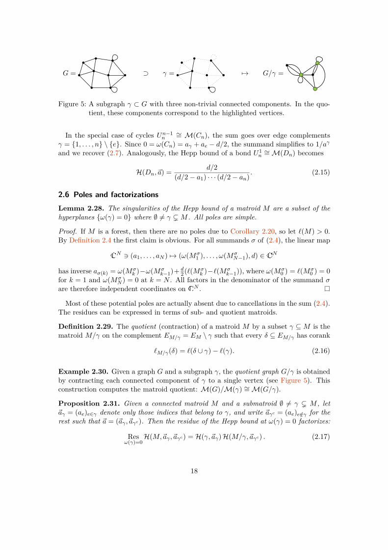
G = ⊃ γ = 7→ G/γ =

Figure 5: A subgraph γ ⊂ G with three non-trivial connected components. In the quo-tient, these components correspond to the highlighted vertices.

In the special case of cycles Un−1n

∼= M(Cn), the sum goes over edge complementsγ = 1, . . . , n \ e. Since 0 = ω(Cn) = aγ + ae − d/2, the summand simplifies to 1/aγand we recover (2.7). Analogously, the Hepp bound of a bond U1

n∼=M(Dn) becomes

H(Dn,~a) = d/2(d/2− a1) · · · (d/2− an) . (2.15)

2.6 Poles and factorizationsLemma 2.28. The singularities of the Hepp bound of a matroid M are a subset of thehyperplanes ω(γ) = 0 where ∅ 6= γ (M . All poles are simple.

Proof. If M is a forest, then there are no poles due to Corollary 2.20, so let `(M) > 0.By Definition 2.4 the first claim is obvious. For all summands σ of (2.4), the linear map

CN 3 (a1, . . . , aN ) 7→ (ω(Mσ1 ), . . . , ω(Mσ

N−1), d) ∈ CN

has inverse aσ(k) = ω(Mσk )−ω(Mσ

k−1)+ d2(`(Mσ

k )−`(Mσk−1)), where ω(Mσ

0 ) = `(Mσ0 ) = 0

for k = 1 and ω(MσN ) = 0 at k = N . All factors in the denominator of the summand σ

are therefore independent coordinates on CN .

Most of these potential poles are actually absent due to cancellations in the sum (2.4).The residues can be expressed in terms of sub- and quotient matroids.

Definition 2.29. The quotient (contraction) of a matroid M by a subset γ ⊆M is thematroid M/γ on the complement EM/γ = EM \ γ such that every δ ⊆ EM/γ has corank

`M/γ(δ) = `(δ ∪ γ)− `(γ). (2.16)

Example 2.30. Given a graph G and a subgraph γ, the quotient graph G/γ is obtainedby contracting each connected component of γ to a single vertex (see Figure 5). Thisconstruction computes the matroid quotient: M(G)/M(γ) ∼=M(G/γ).

Proposition 2.31. Given a connected matroid M and a submatroid ∅ 6= γ ( M , let~aγ = (ae)e∈γ denote only those indices that belong to γ, and write ~aγc = (ae)e/∈γ for therest such that ~a = (~aγ ,~aγc). Then the residue of the Hepp bound at ω(γ) = 0 factorizes:

Resω(γ)=0

H(M,~aγ ,~aγc) = H(γ,~aγ)H(M/γ,~aγc) . (2.17)

18

Proof. Note that |M | ≥ 2, so we must have `(M) ≥ 1 forM to be connected. The linearfunction `(M)ω(γ) = ~a ·~c of ~a has exactly two different coefficients, ce = `(M)− `(γ) fore ∈ γ and ce = −`(γ) when e /∈ γ. Only one other submatroid yields the same partition,namely the complement γc = M \γ. But ω(γ) and ω(γc) are linearly independent, since

det(`(M)− `(γ) −`(γ)−`(γc) `(M)− `(γc)

)= `(M)

[`(M)− `(γ)− `(γc)

]6= 0

because `(M) = `(γ) + `(γc) would imply that M ∼= γ ⊕ γc is disconnected. It followsthat a summand σ in (2.4) is singular on ω(γ) = 0 only if its flag goes through γ = Mσ

k

at k = |γ|. So α := σ|1,...,k is a permutation of γ, and we can view β := σ|k+1,...,N asa permutation of the quotient Q := M/γ. We can therefore write

Resω(γ)=0

H(M,~a) = Resω(γ)=0

( ∑α∈Sγ

χ(∆αω)) 1ω(γ)

( ∑β∈SQ

N−k−1∏i=1

1ω(γ) + ω(Qβi )

)

because we have ω(Mσk+i) = ω(γ)+ω(Qβi ) due to (2.16). The sum over α gives H(γ,~aγ),

and similarly we get H(Q,~aQ) from the sum over β, since ω(γ) = 0 on the pole.

Remark 2.32. Formula (2.17) is wrong for disconnected matroids. The forest G = hasa subgraph γ = 1 ∼= with quotient 2 ∼= . The right hand side of (2.17) gives 1for the residue of H(G,~a) = 0 at ω(γ) = a1 = 0. This contradiction arises because alsothe subgraph γ = 2 gives vanishing ω(2) = 0 on ω(γ) = 0, since 0 = ω(G) = a1 +a2.

Corollary 2.33. If M is a connected matroid with at least two edges, and e ∈M , then

Resae=0H(M,~a, ae) = H(M/e,~a) and Res

ae=d/2H(M,~a, ae) = H(M \ e,~a) . (2.18)

Proof. Since M is connected, e is not a self-loop and thus ω(e) = ae. This proves thefirst claim, because H(e , ae) = 1. Similarly, e cannot be a bridge, so we must have`(M \e) = `(M)−1 and therefore ω(M \e) = ω(M)+d/2−ae. Now use ω(M) = 0.

This yields another proof of one half of Theorem 2.19, namely that, ifM is connected,then H(M,~a) is not the zero function. We use the following fact:

Lemma 2.34 ([112, Claim 6.5]). If a connected matroid M and an edge e ∈ M aregiven, then at least one of M \ e and M/e is also connected.

Corollary 2.35. If M is a connected matroid with at least one edge, then H(M,~a) 6= 0.

Proof. The case |M | = 1 of a single edge is H(M,a1) = 1 6= 0. We proceed by inductionover the number of edges. Suppose |M | ≥ 2 and pick any e ∈ M . If M/e is connected,then we know by induction that H(M/e,~a) 6= 0. If M \ e is connected, we may similarlyassume that H(M \ e,~a) 6= 0. In both cases, (2.18) shows that the Hepp bound of Mcannot be the zero function, because it has a non-vanishing residue.

19

Corollary 2.36. The Hepp bound of a connected matroid M has a pole on the hyper-surface ω(γ) = 0 if, and only if, both γ and its quotient M/γ are connected.

Proof. Apply Theorem 2.19 to the right-hand side of (2.17).

Together with Lemma 2.28, this completely characterizes the poles of the Hepp bound:

Definition 2.37. Given a connected matroid M , a singularity of M is a non-emptysubmatroid γ (M such that γ and M/γ are connected. We denote them as the set

SM := ∅ 6= γ (M : γ and M/γ are connected . (2.19)

Corollary 2.38. The Hepp bound of a connected matroid M is a non-zero rationalfunction with simple poles, precisely on the hypersurfaces ω(γ) = 0 for γ ∈ SM .

Example 2.39. All submatroids and quotients of U rn are themselves uniform: If γ ⊆ U rnhas k = |γ| ≤ r elements, then γ ∼= Ukk

∼= (U11 )⊕k; if k ≥ r, then γ ∼= U rk . The respective

quotients are U rn/Ukk ∼= U r−kn−k and U rn/U rk ∼= U0n−k∼= (U0

1 )⊕(n−k). So only individual edgese and their complements ec = 1, . . . , n \ e are singular, such that

SUrn = e , ec : 1 ≤ e ≤ n if we assume 2 ≤ r ≤ n− 2.

The 2n residues on ae = 0 and ae = d/2 in (2.18) are therefore non-zero, and thesepoles of H(U rn,~a) align perfectly with the denominators in the formula (2.14). In thecase r = n− 1 of cycles Un−1

n∼=M(Cn), the edge complements Cn \ e ∼= Pn are paths

and therefore disconnected as matroids, ec ∼= Un−1n−1∼= (U1

1 )⊕(n−1). Therefore,

SUn−1n

= e : 1 ≤ e ≤ n

shows that H(Cn,~a) only has the poles on ae = 0, as is obvious from (2.7). For a bondU1n∼=M(Dn), edges have disconnected quotients U1

n/ e ∼= (U01 )⊕(n−1) and SU1

nconsists

only of the n complements ec. Indeed, we only see poles at ae = d/2 in (2.15).

The precise knowledge of the singularities of the Hepp bound also tells us the facetsof the convergence cone Θ from (2.6). If ω~a(γ) > 0 for all singular γ ∈ SM , then theHepp bound is finite for these indices ~a. Approaching the boundary ∂Θ where the Mellinintegral (1.13) diverges therefore implies that ω~a(γ)→ 0 for at least one singular γ.

Corollary 2.40. The convergence domain of a connected matroid M is equal to thefollowing intersection of half-spaces, and none of these inequalities is redundant:

Θ =⋂

γ∈SM

~a ∈ RN : ω~a(γ) > 0

⊆ RN . (2.20)

This amounts to a well-known description of matroid polytopes, see Corollary 6.11.

20

2.7 Other matroid invariantsAs explained in Remark 2.3, we can recover a connected matroid M from H(M,~a). Inprinciple, every invariant of M can therefore be calculated from its Hepp bound; butin practice it may not be obvious how to achieve this efficiently. It seems worthwhile,then, to identify the aspects of the function H(M,~a) that are encoded in other matroidinvariants, and to exhibit their connection as explicitly as possible. We merely sketch aglimpse here and limit our discussion to the invariants of Crapo and Derksen.Recall that the increments of the superficial degree of convergence associate a sum

Φ(M) :=∑σ∈SM

∆σω ∈ Z⟨ae, ae − d

2 : e ∈M⟩

of words with letters of the form ae and ae − d/2 to every matroid. To obtain the Heppbound, we apply the map χ or χ from (2.10) and (2.11) to this sum,

H(M,~a) = Resω(M)=0

χ(Φ(M)) = χ(Φ(M))|ω(M)=0.

If we set all indices to ae = 1, then the words in Φ(M) contain only two letters, 〈1〉 and〈1− d/2〉. This specializes at d = 2 to the invariant studied by Derksen [52],

G (M) :=∑σ∈SM

〈rk(Mσ1 ), rk(Mσ

2 )− rk(Mσ1 ), . . .〉 ∈ Z 〈0, 1〉 (2.21)

which is universal for valuative matroid invariants [53] with values in Q. It thus deter-mines several other matroid invariants, like the Tutte polynomial [41], however it cannotdistinguish all non-isomorphic matroids [52, Example 3.5]. It is thus impossible to re-construct the full Hepp bound function H(M,~a) from G (M), but, whenever defined, wefind the special value H(M) at unit indices ae = 1.

Example 2.41. Every order on the uniform matroid U rn yields the same rank sequence:

G (U rn) = n! 〈1, . . . , 1︸ ︷︷ ︸r

, 0, . . . , 0︸ ︷︷ ︸n−r

〉.

Example 2.42. Consider the complete graphK4. The first 3 edges γ = σ(1), σ(2), σ(3)of any permutation σ ∈ S6 either form one of the 4 triangles γ ∼= C3, or one of the|TK4 | = 16 spanning trees. The corresponding rank increments are 〈1, 1, 0, 1, 0, 0〉 and〈1, 1, 1, 0, 0, 0〉, respectively. Each of these appears 3! · 3! times for each fixed γ, becausethe edges of γ and its complement may be permuted arbitrarily, and we conclude

G( )

= 144 〈1, 1, 0, 1, 0, 0〉+ 576 〈1, 1, 1, 0, 0, 0〉.

Lemma 2.43. If the Hepp bound (2.4) is defined for unit indices, then it can be obtainedas H(M) = h(G (M)) from Derksen’s invariant, via a linear map h defined on words as

h(〈r1, . . . , rn〉) :=n−1∏k=1

1k − d

2∑

1≤j≤k(1− rj)where d

2:= n∑n

k=1(1− rk).

21

Proof. With rk = rk(Mσk )− rk(Mσ

k−1) we get `(Mσk ) = k− rk(Mσ

k ) = k− (r1 + · · ·+ rk),such that ω(Mσ

k ) = k − d2∑kj=1(1− rj) in (2.4).

Example 2.44. From h(1, 1, 0, 1, 0, 0) = 1/4 and h(1, 1, 1, 0, 0, 0) = 1/12 we infer thatH(K4) = h(G (K4)) = 144/4 + 576/12 = 84 as claimed in (1.9).

Crapo [40] defined a non-negative integer β (M) ∈ Z≥0 for every matroid M as

β (M) = (−1)rk(M) ∑γ⊆M

(−1)|γ| rk(γ). (2.22)

This is the coefficient of x in the Tutte polynomial TM (x, y) and it also appears as thefirst coefficient of Speyer’s invariant [106]. Some of its remarkable properties are:

1. WhenM has at least two edges, then β (M) = 0 precisely whenM is disconnected.

2. If M has at least two edges and M? denotes its dual, then β (M?) = β (M).

3. For a 2-sum (see Definition 4.8), β (A e⊕f B) = β (A)β (B) is multiplicative [30].

We already saw that the Hepp bound shares the same vanishing property, and section 4proves that it also behaves in the same way for duals and 2-sums. This very close analogysuggests that Crapo’s invariant is a special value of the Hepp bound, and indeed it is.

Lemma 2.45. The Hepp bound of a connected matroid M on N ≥ 2 edges vanishes tofirst order on the hyperplane a1 + · · ·+ aN = 0 where d = 0. Concretely, assume thatω(γ)→

∑e∈γ ae 6= 0 stays non-zero in the limit d→ 0, for all non-empty γ (M . Then

H(M,~a) = d/2a1 · · · aN

(−1)`(M)+1β (M) +O(d2) as d→ 0. (2.23)

Proof. Since aγ :=∑e∈γ ae 6= 0, we may expand 1/ω(γ) = 1/aγ + d

2`(γ)/a2γ +O(d2) for

small d. The Hepp bound (2.4) thus becomes

H(M,~a) =∑

σ∈SM

χ(aσ(1), . . . , aσ(N))

1 + d

2

N−1∑k=1

`(Mσk )

aMσk

+O(d2).

Because of a1 + · · ·+ aN = d2`(M) and (2.12), the first summand in braces gives

∑σ∈SM

(aσ(1) + · · ·+aσ(N))χ(aσ(1), . . . , aσ(N)) = d

2`(M)χ(〈a1〉 . . . 〈aN 〉) = d

2`(M)

a1 · · · aN.

We group the remaining summands in braces by the submatroidMσk . To obtainMσ

k = γ,the first k = |γ| elements of σ must form a permutation τ of γ, and the remaining N −kedges ρ permute the complement M \ γ. All these contributions can thus be written as

d

2`(γ)∑τ∈Sγ

χ(aτ(1), . . . , aτ(k))∑

ρ∈SM\γ

χ(aγ , aρ(1), . . . , aρ(N−k)).

22

The sum over τ is a shuffle product and equals 1/(∏e∈γ ae) according to (2.12). For τ ,

we use the antipode (2.13) to rewrite the summand as (−1)N−kχ(aρ(N−k), . . . , aρ(1)) andsee a shuffle product again. Collecting all contributions, we obtain

H(M,~a) = d/2a1 · · · aN

∑∅6=γ⊆M

(−1)N−|γ|`(γ) +O(d2).

With rk(γ) = |γ| − `(γ), we recognize Crapo’s definition (2.22).

Example 2.46. From (2.7) and (2.15), we see that cycles and bonds have beta invariantβ (M(Cn)) = β (M(Dn)) = 1. More generally, note that β (M) = 1 if and only if M isseries–parallel [40, Proposition 8].

In Definition 4.1 we introduce a variation H(M,~a) of the Hepp bound, that evaluatesat d = 0 precisely to (−1)rk(M)+1β (M). We can derive the above facts 1. through 3. forCrapo’s invariant from the corresponding symmetries of the Hepp bound H(M,~a).However, this argument does not apply to completion (see Remark 4.27), and Crapo’s

invariant violates this symmetry. For example, the graphs from Figure 1 give the values

β

( )= 4 6= 6 = β

( ). (2.24)

These are computed with the contraction-deletion formula β (M) = β (M/e) +β (M\e),which applies whenever e is neither a self-loop nor a bridge [40, Theorem I].

3 Flag formulasThe formula (2.4) has N ! summands, one for each flag ∅ 6= γ1 ( · · · ( γN = G ofsubgraphs γk = Gσk . This is very inefficient and hides the structure and simplicity ofresults like (2.7). Below we will partition all flags into families of subsets that are easilysummed, and thereby derive expressions for the Hepp bound with much fewer terms.In subsection 3.1 we give a formula summing over flags of bridgeless matroids, which is

particularly efficient for small loop number ` and for example gives (2.7) on the nose asa single term. It yields an algorithm that computes the Hepp bound in O(N `+2) steps.Dually, flags of flats are most efficient for small ranks, see subsection 3.2.On the level of the integral (1.5), the flag formulas correspond to a decomposition

of the integration domain into fewer sectors, that each combine many individual Heppsectors. In section 5 we apply these sectors to the period itself to get improved bounds.

3.1 Bridges and earsDefinition 3.1. A circuit C ⊆ M of a matroid is a minimal dependent set, and wewrite CM for the set of all circuits. An edge e ∈ EM is called a bridge (also coloop andisthmus) if it is not contained in any circuit; equivalently, if it is contained in every basis.We say that a matroid M is bridgeless (or 1pi) when it does not have any bridges.

23

K4 \ e =e

K4 \ v =

v

K4 \ e, f =e

f

Figure 6: The three types of bridgeless subgraphs of K4 are highlighted (solid edges).

Each bridge e corresponds to a direct summand M |e ∼= U11 of M = (M \ e) ⊕M |e.

Connected matroids are thus always bridgeless, except for M ∼= U11∼= M( ). Our

use of ‘1pi’ as a synonym for bridgeless stems from particle physics, where graphs Gwith bridgeless matroids M = M(G) play a special role and are called 1-particle irre-ducible, see [15, Section 5.8] and [71]. Note that in our terminology, 1pi does not requireconnectedness in any sense: direct sums of bridgeless matroids remain bridgeless.A bridge e is characterized by the equivalent conditions rk(M \ e) = rk(M) − 1 and

`(M \e) = `(M), and hence a bridgeless matroid is a minimal subset for its loop number:

M is bridgeless ⇔ `(M \ e) < `(M) holds for all e ∈ EM .

Let br(M) ⊂ EM denote the set of all bridges of M . Its complement cyc(M) is thelargest bridgeless submatroid of M and it consists of the union of all circuits:

cyc(M) := M \ br(M) =⋃

C∈CM

C. (3.1)

Bridgeless graphs enter the study of Feynman periods through the desingularization ofgraph hypersurfaces, where they are referred to as motic graphs in [24, Definition 3.1]and core graphs in [10]. They label singular loci and after blowing-up, the flags (maximalchains) of bridgeless graphs correspond to the deepest strata of the boundary divisor [9,Lemma 7.4]. It is therefore not surprising that they can also organize the Hepp bound:

Proposition 3.2. For a connected matroid M on N edges with ` = `(M) ≥ 1 loops, let

F1piM := ∅ = γ0 ( γ1 ( · · · ( γ` = M : each γk is bridgeless with `(γk) = k

denote the set of flags of bridgeless submatroids ofM . For any nested subsets δ ⊆ γ ⊆M ,let aγ/δ :=

∑e∈γ\δ ae denote the sum of the indices of the additional edges in γ. Then

H(M,~a) = 1a1 · · · aN

∑γ•∈F1pi

M

aγ1/γ0 · · · aγ`/γ`−1

ω(γ1) · · ·ω(γ`−1) . (3.2)

Example 3.3. Consider the complete graph K4 = on four vertices, with unit indicesa1 = · · · = a6 = 1 and thus in d = 4 dimensions. The only bridgeless subgraphs are:

• six edge complements K4 \ e ∼= with two loops and ω( ) = 5− 42 · 2 = 1,

24

G =

σ(4)

σ(2)

σ(1)

σ(3)

σ(5)

σ(7)

σ(6) →

Gσ4 =

Gσ6 =→

γσ1 =

γσ2 =

Figure 7: In the order σ of the edges of the depicted graph G, the loop number increasesat i1 = 4, i2 = 6 and i3 = 7. The associated flag is γσ1 ⊂ γσ2 ⊂ γσ3 = G.

• four triangles ∼= K4 \ v with ω( ) = 1 from removing a vertex, and

• three squares ∼= K4 \ e, f with ω( ) = 2 by deleting two non-adjacent edges.

These are illustrated in Figure 6, and we can form∣∣F1pi

K4

∣∣ = 18 different flags. They comein two types, and their contributions to the Hepp bound H(K4) = 84 = 6 · 12 + 2 · 6 are

• 3·2·11·1 = 6 for each of the 12 flags ⊂ ⊂ , and

• 4·1·12·1 = 2 for each of the 6 flags ⊂ ⊂ .

Remark 3.4. Every biconnected graph admits a flag of biconnected (hence bridgeless)graphs [116, Theorem 19], as in the example above. Such flags are called open eardecompositions, and this notion generalizes to connected matroids. However, the sum(3.2) will typically involve more general bridgeless flags, as in Figure 7 (γσ2 is separable).

Proof of Proposition 3.2. Each permutation σ ∈ SM defines a bridgeless flag as follows(see Figure 7): Let i1 < . . . < i` denote the positions of edges that add a loop:

`(Mσik

) = 1 + `(Mσik−1) for every 1 ≤ k ≤ `.

The corresponding bridgeless subsets γσk = cyc(Mσik

) ⊆Mσik

give rise to a map

FM : SM −→ F1piM , σ 7→ (γσ1 ( · · · ( γσ` ) ,

and we ask which permutations σ lie in the preimage of a given bridgeless flag γ• ∈ F1piM .

The last edge e = σ(N) ∈ S := M \M ′ must belong to the complement of M ′ := γ`−1,and all remaining edges S \ e are bridges of M \ e. Those may appear in any orderand at arbitrary positions in σ, without changing the associated bridgeless flag. So if wewrite σ′ for the order of the edges of M ′ as they appear in σ and we fix some τ ∈ SM ′

with FM ′(τ) = γ′• := (γ1 ( · · · ( M ′), then the set σ ∈ SM : σ′ = τ and σ(N) = e isin bijection with the shuffles of τ and the elements of S \ e. The sum over these σ is

∑FM (σ)=γ•

χ (∆σω) =∑

FM′ (τ)=γ′•

∑e∈S

χ

(∆τω

e 6=f∈Saf

)

=aM/M ′

aS1

ω(M ′)∑

FM′ (τ)=γ′•

χ (∆τω)

25

D3(i, j, k) =1

2 i

j

k

1

1

2 K−3,3 = K3,3 =

Figure 8: The family D3(i, j, k) of all biconnected two-loop graphs, the complete bipar-tite graph K3,3 and its depletion K−3,3 = K3,3 \ e by one edge.

with aS :=∏e∈S ae, where we used the multiplicativity (2.12). This reduces the sum

over σ ∈ F−1M (γ•) to the preimages τ ∈ F−1

M ′ (γ′•) of the truncated flag γ′• of length `− 1,and iteration of this rule eventually leads to (3.2).

The length of the bridgeless flags is given by the loop number `, and hence the formula(3.2) tends to be particularly efficient for small `. In particular, the case M = UN−1

N∼=

M(CN ) of a single loop results in a unique flag and gives directly the result (2.7).

Example 3.5. The two-loop graphs D3(i, j, k) from Figure 8 consist of three paths withi, j and k edges between shared endpoints. Their only bridgeless subgraphs are the threecycles Cj+k, Ci+k and Ci+j that are left over after deleting the edges of one of the paths.Hence the sum in (3.2) has merely three terms, and for unit indices we obtain

H(D3(i, j, k)) = i(j + k)j + k − d/2 + j(i+ k)

i+ k − d/2 + k(i+ j)i+ j − d/2 . (3.3)

In more interesting cases, however, the number of bridgeless flags can become huge:Fix a basis b ∈ BM and consider an order τ of its complement EM \ b = τ(1), . . . , τ(`).Let Cτk denote the unique circuit contained in b ∪ τ(k), then γτk := Cτ1 ∪ . . . ∪ Cτk isbridgeless for each 1 ≤ k ≤ `, with `(γτk ) = k loops, and so we obtain a bridgeless flagγτ• ∈ F

1piM . Since τ(k) = γτk \(γτk−1∪b), this construction yields an injection S` → F1pi

M

and we conclude that every matroid has |F1piM | ≥ `! bridgeless flags.

But it is not necessary to explicitly enumerate the flags, due to the recursive structureof (3.2): Summing only over the penultimate element γ = γ`−1 of the flag, we see that

H(M,~a) =∑

bridgeless γ⊂Mwith `(γ)=`(M)−1

aM/γ

aγcHd(γ,~a)ω(γ) (3.4)

where the subscript in Hd(γ) indicates that this Hepp bound is to be computed in thedimension d determined by ω(M) = 0. This gives a result different from the actual Heppbound H(γ) of γ by itself, since the latter imposes another dimension where ω(γ) = 0.Remark 3.6. We may expand γ in (3.4) into its connected components, similar to (3.11).

Example 3.7. The smallest non-graphic regular matroid is called R10 [102]. It has rank5 and may be represented by the 10 vectors ~ei +~ej +~ek : 1 ≤ i < j < k ≤ 5 ⊂ F5

2 over

26

the field F2 = Z/2Z with two elements. The complement of every edge e is isomorphicto the graphic matroid R10 \ e ∼= M(K3,3) of the complete bipartite graph K3,3. Withunit indices, ω(R10) = 0 in d = 4 dimensions, and hence the Hepp bound of R10 is

H(R10) = 10 · H4(K3,3)ω(K3,3) = 10 · H4(K3,3) = 10 · 9 ·

H4(K−3,3)ω(K−3,3)

= 45 · H4(K−3,3)

in terms of the graphK−3,3 ∼= K3,3\e depicted in Figure 8. It has two bridgeless subgraphsof the form D3(2, 2, 2) = and four subgraphs isomorphic to D3(3, 1, 3) = , hence

H4(K−3,3

)= 2 · 2 · H4( )

ω( ) + 4 · 1 · H4( )ω( ) = 4 · 12

2 + 4 · 27/23 = 42

according to (3.3) and we conclude that H(R10) = 45 · 42 = 1890.

Remark 3.8. The recursion underlying (3.4) can also be applied to the Derksen invari-ant: Indeed, the proof of Proposition 3.2 readily demonstrates that G (M) is completelydetermined by the lattice L1pi

M of its bridgeless submatroids, and we have

G (M) =∑

bridgeless γ⊂M`(γ)=`(M)−1

|M/γ|! ·[G (γ) 〈1〉|M/γ|−1

]〈0〉. (3.5)

From an algorithmic point of view, this method to compute the Hepp bound can beimplemented as a traversal of the Hasse diagram of the lattice

L1piM := ∅ ⊆ γ ⊆ EM : γ is 1pi

of bridgeless submatroids. Starting from its maximum, which is M itself, this latticecan be explored efficiently in a top-down approach as follows:Given a bridgeless matroid γ, we call two edges e and f equivalent if e is a bridge of

γ \ f, in other words, if rk(γ \ e, f) < rk(γ). This is an equivalence relation, andwe can compute the corresponding partition Eγ = S1 t . . . t Sk into equivalence classesSi using less than |γ|2 calls to the rank function. The bridgeless submatroids of γ withloop number `(γ) − 1, that is the maximal elements below γ in L1pi

M , are precisely thecomplements γ \ Si. So the recursion (3.4) has k ≤ |γ| summands.

Corollary 3.9. Let K = |L1piM | ≤ 2N . Then the Hepp bound of M can be computed in

O(K ·N2) many steps, provided that the K values of Hd(γ,~a) can be stored in memory.

We stress that the lattice L1piM grows slowly from the top down: each element γ has

at most |γ| children in the Hasse diagram. In contrast, there is no such bound in thebottom-up direction: For example, the number of circuits (sets directly above ∅ ∈ L1pi

M )in a connected matroid can be exponentially large (take cycles in complete graphs).

Corollary 3.10. Every connected matroid with N elements and ` loops has at mostN(N −1) · · · (N − `+1) bridgeless flags. Consequently, the Hepp bound of matroids withbounded loop number is computable in polynomial time in N .

27

⊃

W7 C7 t P1 P6 t F1 P3 t F4 P1 t F6

Figure 9: Some cuts of the wheel with seven spokes. The dashed edges are cut andseparate the wheel into two parts, indicated by differently drawn vertices.

More formally, if the matroid is given by its rank function as an oracle, then O(N `+2)oracle calls are sufficient to determine the Hepp bound. By Corollary 6.8, this gives apolynomial time algorithm for the calculation of the volume of the polar of the matroidpolytope. For matroids polytopes themselves, such a result is well known [49].

3.2 Flats and cutsDefinition 3.11. A subset γ ⊆ EM of a matroid is called a flat (or closed) if it ismaximal for its rank, so that rk(γ∪e) > rk(γ) for every e ∈ EM\γ. The set of flats ofMforms a lattice Lflat

M , and the span or closure of a subset γ of EM is the unique minimalflat span(γ) that contains γ. The flats γ with rk(γ) = rk(M)− 1 are called hyperplanes(also copoints), and the complements M \ γ of hyperplanes are the cocircuits.

In the case of graphic matroids, a flat is a subgraph γ ⊂ G such that each connectedcomponent δ of γ is (vertex-)induced, saying that δ contains all edges of G that haveboth endpoints in δ. The hyperplanes γ of a connected graph G consist of precisely twocomponents and correspond to vertex bipartitions VG = S t T (cuts) for which bothparts S, T 6= ∅ induce connected subgraphs. Hence, hyperplane complements (circuits)G \ γ are the minimal edge-cuts, also called bonds [109, 110]. For 3-connected G, thevertex complements G \ v are precisely the connected hyperplanes [94, Theorem 1].

Example 3.12. The wheel graph Wn with n = `(Wn) spokes and loops has essentiallytwo types of minimal cuts, see Figure 9: Either the hub is dissected from the entire rimcycle Cn, or a path Pk on k vertices in the rim gets separated from a fan Fn−k.

The minimal element of LflatM is the unique flat of rank zero, namely the set span(∅)

which consists of the self-loops of M . For M connected with rank at least one, this isthe empty set. In this case, the set of flags (maximal chains) of flats is

FflatM :=

∅ = γ0 ( γ1 ( · · · ( γrk(M) = M : each γk is a flat with rk(γk) = k

.

These flags are known to encode a matroid in a very interesting way and have receivedmore attention than the bridgeless case [16, 67]. Our following observation that the flagsof flats directly determine the Hepp bound is very much in the spirit of [14, 67].Remark 3.13. In the position space theory of Feynman integrals [6, 8], flats of Feynmangraphs are called saturated graphs and used to define an arrangement of linear spacesthat are blown up to obtain a wonderful compactification.

28

Proposition 3.14. For a connected matroid M on N edges with rank r = rk(M) ≥ 1,

H(M,~a) = 1a?1 · · · a?N

∑γ•∈Fflat

M

a?γ1a?γ2/γ1

· · · a?M/γr−1

ω(γ1) · · ·ω(γr−1) (3.6)

where a?γ/δ :=∑e∈γ\δ a

?e denotes the sum of the dual indices a?e := d

2 − ae of all edges ofγ that are not already in δ ⊂ γ (see also subsection 4.1).

Proof. Given an order σ ∈ SM , consider the positions i1 < . . . < ir of the edges whichincrease the rank: rk(Mσ

ik) = 1 + rk(Mσ

ik−1). The flats γσk := span(Mσ

ik) form a flag

(γσ1 ( · · · ( γσr ) ∈ FflatM

and we like to sum over all permutations σ that produce a given, fixed flag γ• ∈ FflatM .

Since M has no self-loops, note i1 = 1 so ∆σω starts with 〈ae〉 for e := σ(1). To satisfyγσ1 = γ1, we must have e ∈ γ1. The remaining edges f ∈ γ1 \ e each add a loop andincrement the superficial degree of convergence by af − d

2 . Their positions in σ do notaffect the flag γσ• . So if we fix the order τ = σ|M\γ1 of the edges not in γ1 and write u forthe subsequence of ∆σω given by their increments, then the sum over such σ contributes∑

e∈γ1

χ

(〈ae〉

(u

f∈γ1\e〈af − d

2〉))

=∑e∈γ1

χ

(Su

f∈γ1\eS〈af − d

2〉).

Here we reversed the order of arguments using (2.13) and passed from χ to χ, whichdrops the final letter S〈ae〉 = −〈ae〉. Exploiting the multiplicativity (2.12), this is

= χ((Su)〈ω(γ1)〉

) ∑e∈γ1

∏f∈γ1\e

1a?f

= χ(〈ω(γ1)〉u

) a?γ1∏f∈γ1 a

?f

,

where we inserted the final letter 〈ω(γ1)〉 in order to balance the word and apply (2.13)once more. This argument iterates and proves the claim: At the next step, we considerthe first letter of u = 〈aτ(1)〉u′ and sum over τ(1) ∈ γ2 \γ1, writing χ

(〈ω(γ1)〉〈aτ(1)〉u′

)=

1ω(γ1) χ

(〈ω(γ1) + aτ(1)〉u′

)= 1

ω(γ1)χ(Su′) to then apply the analogous steps as above.

The formula (3.6) is most efficient for matroids of low rank. For bonds U1n, it gives a

single term (d/2)/∏e a

?e, which reproduces (2.15). Dually to subsection 3.1, the lattice

of flats grows slowly from the bottom up: each flat γ ∈ LflatM is covered by at most |M \ γ|

flats, namely span(γ ∪ e1), . . . , span(γ ∪ ek) where M \ γ = e1, . . . , ek.

Corollary 3.15. A connected matroid on N elements with rank r has no more thanN(N − 1) · · · (N − r + 1) flags of flats. The Hepp bound of matroids with bounded rankcan be computed in polynomial time in N .

For computations it is convenient to exploit the recursive structure of (3.6): Let us de-note by Hflat

d (M,~a) the result of this formula in a fixed dimension d, lifting the constraintω(M) = 0. Since the penultimate element γr−1 of a flag of flats is a hyperplane,

Hflatd (M,~a) =

∑hyperplane γ⊂M

Hflatd (γ,~a)ω(γ)

a?M/γ∏e/∈γ a

?e

. (3.7)

29

n d f3 f4 f5 f6 H(Kn)

3 6 3 34 4 3 14 845 10

3 3 11 2654

5·37·5325

6 3 3 10 1303 312 216 · 32 · 5 · 13

f3 = 3f4 = 8n−18

n−3

f5 = 5(n−2)(25n−72)6(n−3)(n−4)

f6 = 3(n−2)(36n3−323n2+948n−900)2(n−3)2(n−4)(n−5)

Table 1: The Hepp bounds of complete graphs with up to n = 6 vertices.

If M = A ⊕ B is a direct sum, its flats α ∪ β ∈ LflatA⊕B

∼= LflatA × Lflat

B are pairs of flatsα, β of the summands. Consequently, the flags Fflat

M are in bijection with the shuffles offlags in Fflat

A with flags in FflatB . The multiplicativity (2.12) then shows that

Hflatd (A⊕B,~a)ω(A⊕B) = H

flatd (A,~a)ω(A) · H

flatd (B,~a)ω(B) . (3.8)

Example 3.16. For a forest γ ∼= Unn∼= (U1

1 )⊕n, the formula (3.6) is easily evaluated to

Hflatd (γ,~a)ω(γ) = 1

a1 · · · anwhere ω(γ) = a1 + · · ·+ an, (3.9)

using either (3.7) or (3.8). The hyperplanes of the cycle M = M(Cn) ∼= Un−1n are

precisely the forests γ = M \ e, f obtained by deleting any pair of edges. So by (3.7),

Hflatd (Cn,~a) =

∑1≤e<f≤n

( ∏k 6=e,f

1ak

)a?e + a?fa?ea

?f

= 1a1 · · · an

∑e

aea?e

∑f 6=e

af . (3.10)

Note that the sum over f gives ω(Cn) + a?e, such that the double sum can be written asd2 + ω(Cn) + ω(Cn)

∑eaea?e. So we recover (2.7) in the dimension where ω(Cn) = 0.

Corollary 3.17. Let M denote a matroid of rank rk(M) ≥ 1, and given any submatroidγ ⊂M , write γ = γ1 ⊕ · · · ⊕ γκ for its κ = κ(γ) connected components. Then

Hflatd (M,~a) =

∑hyperplane γ⊂M

a?M/γ∏e/∈γ a

?e

κ(γ)∏k=1

Hflatd (γk,~a)ω(γk)

. (3.11)

Example 3.18. The complete graph Kn has `(Kn) =(n−1

2)loops and for unit indices

we find ω(Kn) =(n

2)− d

2(n−1

2). Every cut consists of two smaller complete graphs, hence

(3.11) yields a quadratic recursion. We can state it as follows: Set d = 2nn−2 and define

f2 := 1 and fk := kfk−1ω(Kk−1) +

k−2∑i=2

ifi

ω(Ki)fk−i

ω(Kk−i)for 3 ≤ k ≤ n,

then H(Kn) = (n− 1)!(d2 − 1)−`(Kn)fn. We give the results for small n in Table 1.

30

⊃

F6 P6 P2 t F4 F2 t P3 t F1

Figure 10: Some cuts of the fan with 6 spokes and the corresponding blockdecomposition.

We use the recursion (3.11) also to compute the Hepp bounds of all wheels. Recallthat for graphs, the sum over hyperplanes γ is a sum over minimal cuts, and the productover k runs over the biconnected components (blocks) of γ. The computation is tractablebecause a wheel has only few connected flats (induced biconnected subgraphs).

Proposition 3.19. The Hepp bounds of the wheel graphs with unit indices are

H(Wn) = 2nn− 2 + 1

4n−1

n∑k=1

(2n− 2kn− k

)(2kk

)k · 9n−k for every n ≥ 3, (3.12)

and they grow asymptotically like H(Wn) ∼ 3·9n8√

2πn for large n. Their generating functionW (z) :=

∑∞n=3H(Wn) zn = 84z3 + 572z4 + 13240

3 z5 + 35463z6 +O(z7) has the form

W (z) = 2z1− z − 4z − 14z2 − 4z2 log(1− z) + 2z√

(1− 9z)(1− z)3 . (3.13)

Proof. For unit indices, the wheelWn is defined in dimension d = 4 and thus a?e = ae = 1for all 2n edges. As illustrated in Figure 9, for a wheel the recursion (3.11) gives

H(Wn) = nHflat

4 (Cn)ω(Cn) + n

n−1∑k=1

(k + 2)Hflat4 (Fn−k) , (∗)

where the first factor of n is the size of the cut (all spokes) and the factor n in frontof the sum over k accounts for the different copies of the fan Fn−k with n − k spokesobtained by rotations. Note that the paths Pk in the rim give the trivial contributionHflat

4 (Pk) /ω(Pk) = 1 from (3.9), and every fan has ω(Fn−k) = 1. Let us write

C (z) :=∞∑n=3

Hflat4 (Cn)ω(Cn) zn =

∞∑n=3

n(n− 1)n− 2 zn = z3(4− 3z)

(1− z)2 − 2z2 log(1− z)

for the generating function of the cycles according to (3.10), and F (z) :=∑n≥1Hflat

4 (Fn) znfor the generating series of the fans. Then the recurrence (∗) can be written as

W (z) = zddz

(C (z) + z(3− 2z)

(1− z)2 F (z)− 3z2), (†)

31

where the factor in front of F (z) is∑∞k=1(k + 2)zk. To determine F (z), consider the

cuts of a fan as illustrated in Figure 10 and apply (3.11) to obtain the recurrence

Hflat4 (Fn) = n+ 2

n−1∑k=1

(n− k + 1)Hflat4 (Fk) +

∑1<j≤k<n

(k − j + 3)Hflat4 (Fj−1)Hflat

4 (Fn−k)

where the first term stems from dissecting the rim Pn from the hub, the middle sum cutsoff a smaller fan Fk from a path Pn−k in the rim, and the double sum enumerates thecuts that carve out a path in the rim from spoke j to spoke k, chopping off two smallerfans Fj−1 and Fn−k. For the generating function F (z), this recursion reads

F (z) = z

(1− z)2 + 2z(2− z)(1− z)2 F (z) + z(3− 2z)

(1− z)2 F 2(z).

Inserting the solution F (z) = 1−6z+3z2

2z(3−2z) −√

(1−9z)(1−z)3

2z(3−2z) into (†) confirms (3.13), and weobtain (3.12) using the binomial series. The asymptotics for large n can be computedwith standard methods, see [61].

Remark 3.20. If all indices ae = 1 are equal, the partition of all permutations accordingto the first flat γ = span(σ(1)), as described in the proof of Proposition 3.14, amountsto a recursion for the Derksen invariant of the form

G (M) =∑

γ∈LflatM

rk(γ)=1

|γ|! · 〈1〉[〈0〉|γ|−1

G (M/γ)]. (3.14)

We conclude that G (M) is completely determined by the lattice of flats of M , becausethe flats Lflat

M/γ∼= δ ∈ Lflat

M : δ ⊇ γ of a quotient M/γ are precisely those flats δ of Mthat contain γ. This dual to Remark 3.8 was observed in [14, Section 3].

Example 3.21. Starting from the 3- and 4-bonds G( )

= 6〈1, 0, 0〉 and G( )

=24〈1, 0, 0, 0〉, and using 〈0〉〈1, 0, 0〉 = 〈0, 1, 0, 0〉+3〈1, 0, 0, 0〉, the recursion (3.14) gives

G( )

= 〈1〉[G( )

+ 2 · 2! · 〈0〉 G( )]

= 96〈1, 1, 0, 0, 0〉+ 24〈1, 0, 1, 0, 0〉.

Inserting this into G( )

= 6 · 〈1〉 · G ( ) confirms the result from Example 2.42.

3.3 Cyclic flatsIn the preceding two sections, we partitioned the total orders of the edges accordingto the corresponding flags γ• of bridgeless or flat matroids. The corresponding iteratedquotients are cycles γk/γk−1 ∼= Un−1

n or bonds γk/γk−1 ∼= U1n on n = |γk/γk−1| elements,

respectively.Combining both approaches, we can give a formula in terms of only those submatroids

that are simultaneously cyclic (bridgeless) and flat. These form the lattice

ZM := L1piM ∩ L

flatM (3.15)

32

of cyclic flats, and in fact this lattice, together with the rank function, determines thematroid [13, 31]. Note that the closure span(γ) ∈ ZM of any bridgeless γ ∈ L1pi

M , as wellas the interior cyc(γ) ∈ ZM of any flat γ ∈ Lflat

M , are cyclic flats.

Proposition 3.22. The Hepp bound of a connected matroid M fulfils the recursion

Hflatd (M,~a) =

∑M 6=Z∈ZM

Hflatd (Z,~a)ω(Z) ρ (M/Z,~a) (3.16)

over cyclic flats Z (M , in terms of a sum over independent hyperplanes of Q = M/Z:

ρ (Q,~a) :=∑

hyperplane H⊂Qwith `(H)=0

a?Q/H

( ∏e∈H

1ae

)( ∏e∈Q\H

1a?e

). (3.17)

Proof. Given a hyperplane γ of M , let Z := cyc(γ) ∈ ZM denote the cyclic flat thatis the interior of γ. The bridges B := γ \ Z of γ form an independent set such thatγ = Z ⊕B is a direct sum. Using (3.9) and (3.8), we find

Hflatd (γ,~a)ω(γ) = H

flatd (Z,~a)ω(Z)

∏b∈B

1ab.

Together with (3.7) this proves (3.16): Note thatH := γ/Z is an independent hyperplaneof Q = M/Z, so ρ (M/Z,~a) defined in (3.17) correctly collects the contributions from allhyperplanes γ that give rise to the same interior Z = cyc(γ).

Note that (3.16) sums over all cyclic flats Z—in contrast to (3.11) or (3.4), where therank or loop number are fixed. Correspondingly, iterating the recursion (3.16) expressesthe Hepp bound in terms of all chains of cyclic flats, not just the maximal ones:

H(M,~a) =∑k≥1

∑∅6=Z1⊂···⊂Zk=MZ1,...,Zk∈ZM

ρ (Z1) ρ (Z2/Z1) · · · ρ (M/Zk−1)ω(Z1)ω(Z2) · · ·ω(Zk−1) . (3.18)

Remark 3.23. Since M is connected and thus 1pi, every quotient Q = M/Z is also 1pi.Therefore, if Q ∼= A ⊕ B is disconnected, both A and B must have at least one loop:`(A), `(B) ≥ 1. But a hyperplane H of A⊕B must contain all of A or all of B, and thusH cannot be independent. This shows that ρ (Q,~a) = 0 unless Q is connected.

Example 3.24. The only cyclic flats of the complete graph K4 = are ∅, the fourtriangles, and K4 itself. For a triangle Z = i, j, k ∼= , we can write (3.10) as

Hflatd (Z,~a)ω(Z) = 1

aiajak

(ai + aj + ak

ω(Z) + aia?i

+ aja?j

+ aka?k

).

33

The corresponding quotient Q = K4/Z ∼= is a bond with the unique hyperplane ∅,and (3.17) gives simply ρ (Q,~a) = a?u+a?v+a?w

a?ua?va?w

where u, v, w = K4\Z are the complemen-tary edges. Note that the numerator is a?u+a?v+a?w = d

2−ω(Q) = d2 +ω(Z) = ai+aj+ak

due to 0 = ω(K4) = ω(Z) +ω(K4/Z). The only other contribution to (3.16) is ρ (K4,~a)from Z = ∅, which amounts to summing over the three pairs H = i, j ∼= of non-adjacent edges. In total, we get

H(K4,~a) =∑∼=Z⊂K4

aZ∏e∈Z

ae∏e/∈Z

a?e

(aZω(Z) +

∑e∈Z

aea?e

)+

∑∼=Z⊂K4

a?K4/Z∏e∈Z

ae∏e/∈Z

a?e. (3.19)

Remark 3.25. In the case of unit indices ae = 1 = a?e in d = 4 dimensions, the factor(3.17) becomes just ρ (Q) = (`(Q) + 1) · |independent hyperplanes of Q|. The countof independent hyperplanes can be retrieved from the lattice ZQ of cyclic flats and theirranks, as worked out in detail in [14, section 7].We can repeat the above discussion starting with bridgeless flags instead of flags of

flats: Given γ• ∈ F1piM , we can set Zi := span(γi) ∈ ZM and remove duplicates to obtain

a chain of cyclic flats. The final formula has the same form as (3.18), only the numeratoris altered by replacing the factors ρ (Q,~a) with the sum

ρ (Q,~a) =∑C⊂Q

aC

( ∏e∈C

1ae

)( ∏e∈Q\C

1a?e

)

over spanning circuits (indeed, note that γ1 is a spanning circuit of Z1). These areprecisely the circuits of rank rk(C) = rk(Q), equivalently the circuits with |C| = rk(Q)+1elements, and they are also called Hamiltonian circuits. For unit indices ae = 1 in d = 4dimensions, we conclude ρ (Q) = (rk(Q) + 1) · |Hamiltonian circuits of Q|.The two resulting formulas (3.18) for H(M,~a) in terms of chains of cyclic flats, one

with ρ’s and the other with ρ’s in the numerator, can be obtained from each other byduality as in subsection 4.1. Namely, the complement of a Hamiltonian circuit is anindependent hyperplane of the dual [17, Theorem 3].

Example 3.26. The uniform matroid M = U rn has only two cyclic flats ZM = ∅,M,such that H(M,~a) = ρ (M,~a) = ρ (M,~a). As every subset H ⊂M of size |H| = r − 1 isan independent hyperplane and every C ⊂M with |C| = r+ 1 is a Hamiltonian circuit,

H(U rn,~a) =∑

|C|=r+1

aC(∏e∈C ae) (

∏e/∈C a

?e)

=∑

|H|=r−1

a?H(∏e∈H ae) (

∏e/∈H a

?e). (3.20)

Note that Proposition 2.27 gives yet another formula for this function.

4 SymmetriesDifferent graphs (or matroids) may integrate to the same period. There is no completecombinatorial description of all such pairs of graphs, but several families of identities areknown. The simplest of these period relations are:

34

1. duality: A planar graph and its dual have the same period.

2. product: The period factorizes for graphs with a 2-separation.

These hold for arbitrary indices and extend to all matroids; proofs are straightforward inSchwinger parameters. In contrast, the following symmetries are only defined for graphsand furthermore subject to constraints on the indices:

3. Fourier split [70]: Duality may be applied to one side of a 3-separation.

4. completion [21]: If G is regular, then P (G\v) is the same for all vertices v.

5. twist [97]: A double transposition along a 4-separation keeps P (G\v) invariant.

The Fourier split generalises the uniqueness relations [73–75] and we include a proof inSchwinger parameters. For completion and twist, all known proofs [97] exploit the repre-sentation (4.4) of the period in position space. Completion and twist are not restricted toregular graphs, but require indices such that each vertex is conformal (Definition 4.16).

In this section we demonstrate that the Hepp bound respects all of the above symme-tries and fulfils exact analogues of the corresponding identities for periods. Our proofs ofthe completion and twist relations exploit the structure of the singularities of the Heppbound as a rational function of the indices ~a, combined with the factorization (2.17) ofresidues.The product, completion and twist identities are most succinctly stated for arbitrary

indices if we use a slight variation of the Hepp bound.

Definition 4.1. The position space Hepp bound H(M,~a) of a matroid M on N edges is

H(M,~a) := a?1 · · · a?Nd/2 H(M,~a) where a?e = d

2 − ae. (4.1)

In d = 4 dimensions with unit indices ae = 1 on all edges, H(M) = 2H(M) differ onlyby a factor of 2. Also recall H(M,~a) |d=0 = 0 from Corollary 2.21, so the denominatorin (4.1) does not create a further pole. Instead, Lemma 2.45 shows that

H(M,~a)→ (−1)rk(M)+1β (M) for d→ 0. (4.2)

Example 4.2. For cycles and bonds (Figure 3), the results (2.7) and (2.15) translate to

H(DN ,~a) = 1 and H(CN ,~a) = a?1 · · · a?Na1 · · · aN

. (4.3)

The motivation for Definition 4.1 is that the period (2.1) is not exactly a Feynmanintegral. The Mellin integral lacks a prefactor

∏e 1/Γ(ae) to become the actual Feynman

integral in momentum space [87]. A Fourier transform turns this into the integral

P(G,~a) :=

∏v 6=0,1

∫Rd

dd~zvπd/2

∏e=v,w∈EG

1‖~zv − ~zw‖2a

?e

~z0=~0, ~z1=~e1

(4.4)

35

G = = → → G? = =

Figure 11: A planar graph G, a planar embedding of the same graph, the dual indicatedby dashed lines, and another (non-planar) drawing of this dual graph G?.

over position vectors ~zv ∈ Rd associated with each vertex, similar to [99, Definition 3.1].Two arbitrary vertices (labelled 0 and 1) get fixed positions: ~0 and a unit vector ~e1. TheFourier transform introduces further Γ-functions [89], and the precise relation is

P(G,~a) = Γ(d/2)Γ(a?1) · · ·Γ(a?N )P (G,~a) . (4.5)

The replacement Γ(s) 7→ 1/s observed in Example 2.2 suggests that (4.1) is the correcttropical analogue of the Feynman integral in position space.In contrast to the Hepp bound H(G) = 2H(G), note that the period in d = 4 dimen-

sions with unit indices ae = 1 is unchanged in position space: P(G) = P (G).

4.1 DualityEvery matroid M (with corank function `) has a dual matroid M? [88] on the sameground set E = EM = EM? , but with the corank function `? : 2E −→ Z≥0 defined by

`?(γ) = `(E \ γ) + |γ| − `(E). (4.6)

Example 4.3. The dual of the uniform matroid U rn is Un−rn .

Example 4.4. For planar graphs G, choose a planar drawing. Construct the planar dualG? by assigning a vertex to each face and connecting neighbouring faces with edges, asin Figure 11. Then the cycle matroidM(G?) is the dual ofM(G).

Proposition 4.5. Let M denote any matroid and set a?e := d2 − ae for each edge. Then

H(M?,~a) = H(M,~a?) . (4.7)

Proof. The superficial degree of convergence of a subset γ ⊆ E in the dual matroid is

ω~a(γ?) =∑e∈γ

ae − d2

(|γ| − `(M) + `(M\γ)

)= −

∑e∈γ

a?e + d2`(M)− d

2`(M\γ)

according to (4.6). The case γ = E shows that ω~a(M?) = −ω~a?(M) both vanish in thesame dimension. Substitute d

2`(M) =∑e∈M a?e in the equation above to conclude that

ω~a(γ?) = ω~a?(M\γ). The contribution to H(M?,~a) from any flag γ1 ( · · · ( γN in (2.4)therefore matches precisely the contribution of the complementary flag E\γN−1 ( . . . (E\γ1 ( E to the Hepp bound H(M,~a?).

36

M

e⊕f M

= M

=M

Figure 12: The 2-sum of two graphs.

Example 4.6. The cycles Cn and the bonds Dn in Figure 3 are duals of each other,and indeed their Hepp bounds (2.7) and (2.15) are related by (4.7).

Remark 4.7. We can read (4.6) as `?(γ) = rk(M)−rk(M\γ). It follows that the bridgelesssubsets of M? are precisely the complements of flats in M and vice-versa. Hence underduality, the bridgeless flag formula (3.2) becomes the sum (3.6) over flags of flats.The identity (4.7) is also very easy to prove with the Mellin integral: The bases of the

dual are the complements BM? = E \ T : T ∈ BM of the bases of M , such that

ΨtrM?(x) = max

T∈BM

∏e∈T

xe =(∏e∈M

xe

)maxT∈BM

∏e/∈T

1xe

=(∏e∈M

xe

)ΨtrM ((1/xe)e∈M ) . (4.8)

Inversion of the Schwinger parameters xe → 1/xe thus transforms the integrands (1.13)of H(M?,~a) and H(M,~a?) into each other. This proves (4.7), and upon replacing Ψtr

with Ψ, the same argument also shows that

P (M?,~a) = P (M,~a?) (4.9)

This well-known relation for periods is called Fourier identity in [97], because it corre-sponds to a Fourier transform in the position space integral (4.4).

4.2 Products and 2-sumsDefinition 4.8. Suppose we are given two connected matroids A and B, each with atleast 3 elements. Let further e ∈ A and f ∈ B denote a choice of edges. Then the 2-sumM = A e⊕f B is the matroid on the disjoint union EM = EA\e t EB\f with bases

BM :=S t T : S ∈ BA\e and T ∈ BB/f or S ∈ BA/e and T ∈ BB\f

. (4.10)

We illustrate the 2-sum for graphical matroids in Figure 12. It amounts to takingthe disjoint union of A\e and B\f , followed by the identification v ∼ v′ and w ∼ w′ ofthe endpoints of e = v, w and f = v′, w′. As the figure shows, we can flip one side(v′ ↔ w′) and thus obtain two different graphs with the same cycle matroid [108, 117].

Example 4.9 (Figure 13). The 2-sum M e⊕f Ukk+1 with a cycle Ukk+1∼= M(Ck+1)

replaces e in M by a path with k edges. This is called a series operation. A paralleloperation is the 2-sum M e⊕f U1

k+1 with a bond, which replaces e by k parallel edges.

37

From (4.10) we see that the rank of a 2-sum is rk(M) = rk(A) + rk(B)− 1, and thus

`(A e⊕f B) = `(A) + `(B)− 1. (4.11)

Suppose we have assigned indices ~a to S := A\e ⊂ M and indices ~b to T := B\f ⊂ M .They determine the dimension d where ω(M) = 0. If we set ae := d

2 − ω(S), then

ω(A) = ω(S) + ω(A/S) = ω(S) + ae − d2 = 0

and similarly, we get ω(B) = 0 for bf := d2 −ω(T ). Note that bf = ω(S) and ae = ω(T ),

because (4.11) shows that ω(M) = ω(S) + ω(T )− d2 .

Proposition 4.10. Given a 2-sum M = A e⊕f B, let ~a and ~b denote variables indexedby the edges in A\e and B\f , respectively. Set ae := ω(B\f) and bf := ω(A\e). Then

H(M,~a,~b) = H(A,~a, ae) · H(B,~b, bf ). (4.12)

Proof. By our definition, A and B are connected, and it follows that M is connected.As an identity of rational functions, it suffices to prove (4.12) locally, so we may assumethat the indices lie in the convergence cone of the Mellin integral (1.13).Let ψA := Ψtr

A\e and φA := ΨtrA/e such that Ψtr

A = max xeψA, φA. We can write

H(A,~a, ae) =∫PA\e

Ω(~a)(φA)d/2

∫ ∞0

xae−1e dxe

(max xeψA/φA, 1)d/2= d/2aea?e

∫PA\e

Ω(~a)ψaeA φ

a?eA

(4.13)

where a?e = d2 − ae, by performing the integral over λ := xeψA/φA as in Example 2.2:∫ ∞

0

λae−1dλ(max λ, 1)d/2

=∫ 1

0λae−1dλ+

∫ ∞1

λae−d/2−1dλ = 1ae

+ 1d/2− ae

= d/2aea?e

.

Set also ψB := ΨtrB\f and φB := Ψtr

B/f , then according to (4.10), we can write the tropicalmatroid polynomial of the 2-sum as Ψtr

M = max ψAφB, φAψB = ψAφB max 1, λ interms of the coordinate λ := (φA/ψA)(ψB/φB) on PM . Combining λ with the forgetfulmaps x 7→ y := [xi]i∈A\e and x 7→ z := [xi]i∈B\f , we obtain a change of variables

PM −→ PA\e ×PB\f ×R>0, x 7→ (y, z, λ). (∗)

Since φA and ψA are homogeneous of degrees `(A) and `(A) − 1, respectively, λ ishomogeneous of degree one in the variables y. Consequently, (∗) is invertible with

x(y, z, λ) =[

λ

λ′(y, z)y : z]∈ PM for λ′(y, z) := φA(y)ψB(z)

ψA(y)φB(z) .

Under this rescaling, ψA(x) = ψA(y)(λ/λ′)`(A\e) and the volume form (2.5) is of degree∑i∈A\e ae = ω(A\e) + d

2`(A\e) in y. With bf = ω(A\e), the integrand factorizes as

Ω(~a,~b)(Ψtr

M (x))d/2= Ω(~a)ψA(y)d/2

(ψA(y)φA(y)

)bf∧ Ω(~b)φB(z)d/2

(φB(z)ψB(z)

)bf∧ λbf−1dλ

(max 1, λ)d/2.

38

e⊕3 = e⊕3 =

Figure 13: Series and parallel operations on edge e, illustrated for graphical matroids.

The integrals over z ∈ PB\f and λ produce precisely H(B,~b, bf ) by the equivalent of(4.13) for B. Since bf = d

2−ae = a?e, the integral of the first term over y gives H(A,~a, ae)times a?eb?f/(d/2), again using (4.13). We have thus shown that

H(M,~a,~b) = a?eH(A,~a, ae) · b?fH(B,~b, bf ) · 2/d,

which becomes the claim (4.12) in position space (4.1).

Example 4.11. Recall that H(K4) = 84 and H(K4) = 42 for unit indices in d = 4dimensions. All 2-sums of K4 with itself are isomorphic, and we find that

H( )

= H(

e⊕f)

= H( )2

= 1764 and H( )

= 3528.

Corollary 4.12 (series–parallel reductions). If the matroid S = M e⊕3 U23 is obtained

from M by replacing an edge e with two edges 1 and 2 in series (Figure 13), then

H(S, a1, a2,~a) = a1 + a2a1a2

H(M,a1 + a2,~a) . (4.14)

If P = M e⊕3 U13 is obtained from M by replacing e with a pair of parallel edges, then

H(P, a1, a2,~a) = a?1 + a?2a?1a

?2H(M,a1 + a2 − d

2 ,~a). (4.15)

In particular, the Hepp bound in position space is invariant under parallel operations:

H(P, a1, a2,~a) = H(M,a1 + a2 − d

2 ,~a). (4.16)

Proof. Apply Proposition 4.10 to B = U23 or B = U1

3 and use (4.3).

Corollary 4.13. Crapo’s invariant of a 2-sum is β (A e⊕f B) = β (A)β (B) [30], andseries–parallel operations do not affect Crapo’s invariant [40, Propositions 4 and 5].

Proof. We use (4.2) and apply the limit d −→ 0 to (4.12). Because of rk(M) − 1 =rk(A)−1+rk(B)−1 from (4.11), this proves the first claim. The series–parallel invarianceis the special case B =M(Cn) or B =M(Dn), with β (B) = 1 due to Example 2.46.

39

The product (4.12) is the exact analogue of the well-known relation [23, Proposition 40]

P(A e⊕f B,~a,~b

)= P(A,~a, ae) · P(B,~b, bf ) (4.17)

for the period in position space. It can be proven in the same way as above; the onlydifference arises because ΨM = ΨA\eΨB/f + ΨA/eΨB\f is a sum and not the maximum.Hence the λ-integrals become Euler beta functions, and the analogue of (4.13) reads

P (A,~a, ae) = Γ(ae)Γ(a?e)Γ(d/2)

∫PA\e

Ω(~a)ΨaeA\eΨ

a?eA/e

.

The product formulas suggest a unique factorization for matroids with respect to 2-sums, and indeed this was achieved in [47]. We review this result and related terminology.

Definition 4.14. A (Tutte) k-separation of a matroid M is a partition EM = S t T ofits edges such that |S| , |T | ≥ k and rk(A) + rk(B) ≤ rk(M) + k − 1. We say that M isn-connected if it has no k-separation where 1 ≤ k < n.

With this definition, every matroid is 1-connected, and a connected matroid accordingto Definition 2.15 is called 2-connected. For a connected graph G, a k-separation ofM(G) is an edge partition with |S| , |T | ≥ k such that S and T meet in at most kvertices [46, Theorem 3]. So Definition 2.17 describes the special case of 1-separations,and Figure 12 shows 2-separations.

In [47], 2-separations are called splits, and a matroid is called prime if it is 3-connected.Every 2-sum decomposition M ∼= A e⊕f B implies the existence of a split with S = A\eand T = B\f . Conversely, every split arises in this way and implies a decomposition ofMinto minors A and B ofM . Therefore, a prime matroid admits no 2-sum decomposition.It follows that a connected matroid is decomposable by 2-sums into prime matroids.

Apart from the order of performing the splits, this decomposition is almost unique. Theonly ambiguity arises from cycles Cn+m ∼= Cn+1 e⊕f Cm+1, and similarly bonds, whichallow several decompositions. The unique factorization result is [47, Theorem 18]:

Theorem 4.15. Every connected matroid has a unique minimal 2-sum decompositioninto bonds, cycles, and 3-connected matroids.

The Hepp bound implements this decomposition as an actual factorization of rationalfunctions. Cycles and bonds (4.3) have only linear factors in the numerator and denom-inator, which may be partitioned in several ways. In contrast, the numerator of H(M,~a)for a 3-connected matroid will not factorize into linear polynomials.

4.3 CompletionThe completion symmetry is the invariance of the integral (4.4) in position space under aconformal transformation ~z 7→ ~z/ ‖~z‖2. It is very useful in particle physics as it equatesthe periods of many non-isomorphic graphs [21, section 5]. Completion applies only tographs and requires that, at each vertex, the dual indices sum up to the dimension.

40

Definition 4.16. Let a?e = d2 − ae denote the dual indices. The excess at a vertex v is

δv := d−∑e : v∈e

a?e (4.18)

where the sum runs over all edges incident to v. We call v conformal if δv = 0, and aconformal graph is a graph G together with indices ~a such that all vertices are conformal.

Example 4.17. Every k-regular graph with k ≥ 3 and unit indices ae = 1 on all edgesis conformal in d = 2k/(k − 2) dimensions. For k = 4, this dimension is d = 4.

Example 4.18. For any graph G with logarithmic indices, its completion [97, 99] isa conformal graph H with one additional vertex ‘∞’ such that G = H\∞. To makev ∈ VG with δv 6= 0 conformal, H has an edge e from v to ∞ with ae := d/2− δv. Thenew vertex ∞ is conformal by virtue of δ∞ = −ω(G) = 0 from (4.19) below.

We can express the convergence degree of a subgraph in terms of excesses. Let G[S]denote the subgraph of G that is induced by the vertex set S ⊆ VG. It contains preciselythose edges of G which have both endpoints in S.

Lemma 4.19. Suppose that γ = G[S] ⊆ G is a connected induced subgraph. Let C ⊂ EGdenote the edges with precisely one endpoint in S. Then

ω(γ) = 12

(∑v∈S

δv +∑e∈C

a?e − d). (4.19)

Proof. The sum∑v∈S

∑e:v∈e a

?e counts edges in γ twice and edges in C once. Hence,∑

v∈Sδv − d |S|+

∑e∈C

a?e = −2∑e∈γ

a?e = −d |γ|+ 2∑e∈γ

ae = 2ω(γ) + d (`(γ)− |γ|)

and we conclude using (2.2).

In particular, a conformal graph has ω(G) = −d/2 and is not logarithmic unless d = 0.However, the complement G\v of any vertex in a conformal graph is always logarithmicwith ω(G\v) = −δv/2 = 0. We can therefore consider the periods of such complements.

Theorem 4.20. If G is conformal, then P(G\v,~a) is the same for all vertices v.

The proof for positive integer dimensions in [97, Definition and Theorem 2.2] appliesthe inversion ~z 7→ ~z/ ‖z‖2 to the vertex coordinates in position space (4.4). In non-integerdimensions, these integrals over ~z ∈ Rd can be defined using dimensional regularizationas explained for example in detail in [35]. The inversion proof then still applies.We will prove the same invariance for the Hepp bound. Recall that the Mellin integrals

(1.13) and (2.1) have poles. The equalities P(G\v,~a) = P(G\w,~a) of Theorem 4.20 areto be understood as identities of meromorphic functions on the vector space⋂

u∈VG

~a : δu = 0 ⊂ C|G|

41

K4 =a1

a2

a3

a1

a2

a3K4\v =

a2

a3a1 H(K4\v,~a) = (a1 + a2)(a1 + a3)(a2 + a3)a1a2a3

Figure 14: The complete graph K4 with the most general conformal indices.

of conformal indices on G. This space has dimension |G| − |VG| + 1 = `(G), becauseone of the constraints determines the dimension d. Even though a complement G\v hasfewer edges than G, we still write ~a to denote its indices and to suggest that the indicesof G\w are determined (through conformality in G) by the indices of G\v.

Theorem 4.21. For any two vertices v, w of a biconnected graph G, the Hepp boundsH(G\v,~a) = H(G\w,~a) agree as rational functions on the space of conformal indices.

Corollary 4.22. If G is regular and G\v, G\w are p-log, then H(G\v) = H(G\w).

Example 4.23. The complete graph K4 is conformal precisely when the indices ae = afof all non-adjacent edge pairs e, f coincide. The conformal indices thus define a rainbowcolouring, where every vertex touches exactly one edge of each index (see Figure 14).All complements give the same cycle C3, so Theorem 4.21 is trivial for G = K4.

To prove the theorem, we first reduce it to the case of complete graphs Kn. If G hasn vertices, define indices ~c on Kn as follows: The edge between vertices i and j receives

c?ij = d2 − cij := a?e1 + · · ·+ a?ek , (4.20)

where e1, . . . , ek ∈ EG denote all edges in G between i and j (there may be none, one,or several such edges). This assignment ensures that ~c are conformal indices for Kn. Soif we know H(Kn\v,~c) = H(Kn\w,~c), then the theorem for G follows from the identity

H(G\v,~a) = H(Kn\v,~c) (4.21)

and its analogue for w. We already saw in (4.16) that several parallel edges (k ≥ 2) canbe replaced by a single edge with the dual index (4.20). Nothing changes for edges withk = 1, so (4.21) is clear once we recognize that adding an edge with weight cij = d/2 inthe case k = 0 has no effect on the Hepp bound. Indeed, due to the factors a?e in (4.1),the pole for deletion of an edge in (2.18) amounts to the finite limit

H(G t e ,~a, d/2) = limae→d/2

H(G t e ,~a, ae) = H(G,~a) .

Lemma 4.24. For a biconnected graph G, the poles of the Hepp bound H(G,~a) inposition space are in bijection with subsets S ( VG of |S| ≥ 2 vertices with the propertythat the induced subgraph γ = G[S] and its quotient G/γ are biconnected.

42

G = γ

v

w

H =u

v

w

G = w

γ

v

γ′

C

H =u

v

Figure 15: An induced subgraph γ = G[S] ( G\v in the cases w /∈ S and w ∈ S.

Proof. According to Corollary 2.38 and Lemma 2.18, the poles of H(G,~a) are identifiedwith subgraphs γ such that γ and G/γ are nonseparable. If γ is not induced, every edgee ∈ G\γ with both endpoints in γ becomes a self-loop in the quotient G/γ. To avoid aseparation, G/γ ∼= can only consist of one self-loop on its own, so γ = G\e is an edgecomplement. But the corresponding poles at ω(G\e) = a?e = 0 are cancelled in positionspace by the numerators in (4.1). So only induced γ contribute poles to H(G,~a).

In a complete graphG = Kn, all induced γ = G[S] and their quotients are biconnected,so H(Kn,~a) has precisely 2n − n − 2 poles, one for each subset S ( 1, . . . , n with|S| ≥ 2. To identify poles in other graphs, it may be useful that the quotient G/G[S] isbiconnected if and only if the complement G\S = G[VG\S] is a connected graph.

Proof of Theorem 4.21. We perform an induction over the number n of vertices of G.The start at n = 3 is simple: All vertex complements of K3 = are single edgesK3\v ∼= with the same Hepp bound H(D1,~a) = 1 from (4.3).

Now consider the complete graph G = Kn+1 and suppose that we already establishedthe theorem for all graphs with ≤ n vertices. Call v = n+1 such that G\v = Kn. Recallfrom Example 4.18 that the indices on Kn are unconstrained and parametrize the entirespace of conformal indices on G, so H(Kn,~a) has simple poles in bijection with subsetsS ( 1, . . . , n of size |S| ≥ 2. In position space, the factorization (2.17) reads

Resω(γ)=0

H(Kn,~a) = d2

[H(γ,~a) · H(Kn/γ,~a)

]ω(γ)=0

(])

and we first consider the case γ = G[S] with w /∈ S (see Figure 15). Then γ is alsoa subgraph of G\w, and we set H := G/γ such that Kn/γ = H\v. The excess of thevertex u representing γ in H is −2ω(γ) due to (4.19). So on the hyperplane ω(γ) = 0,the graph H is itself conformal. Since H has at most n vertices, we know by inductionthat H(H\v,~a) = H(H\w,~a). But H\w = (G\w)/γ, so we learn

Resω(γ)=0

H(G\v,~a) = Resω(γ)=0

H(G\w,~a)

by comparing (]) with its analogue for G\w instead of G\v = Kn. Now suppose thatw ∈ S, then γ = G[S] is not anymore a subgraph of G\w. To see the pole, set γ′ := G[T ]for the complement T := 1, . . . , n+ 1\S and note that ω(γ) = ω(γ′) = (

∑e∈C a

?e−d)/2

by (4.19), where C are the edges between S and T . The residue formula gives

Resω(γ)=0

H(G\w,~a) = Resω(γ′)=0

H(G\w,~a) = d2

[H(γ′,~a

)· H(G\w/γ′,~a

)]ω(γ′)=0

. ([)

43

K4 = K5\5 =

a 1a3

a4

a2

a 6

a5

2

1

4

3

K5\2 =

a 1a3

a35

a45

a 15

a5

5

1

4

3

a45 = 2(a4+a5+a6)−a1−a2−a33

a35 = 2(a1+a2+a6)−a3−a4−a53

a15 = 2(a2+a3+a4)−a1−a5−a63

Figure 16: Two uncompletions of K5 and the relationship of their indices.

This time, we delete from H = G/γ the vertex u that represents γ, to conclude byinduction and H\u = G\S = G[T ] = γ′ that H(G\v/γ,~a) = H(H\v,~a) = H(γ′,~a).Similarly, set H ′ := G/γ′ such that H ′\u′ = G\T = G[S] = γ for the vertex u′ that is γ′in H ′. By induction, we find that H(G\w/γ′,~a) = H(H ′\w,~a) = H(γ,~a) and concludethat (]) and ([) coincide.In summary, we have shown that both Hepp bounds H(G\v,~a) and H(G\w,~a) have

the exact same residues on all poles. Therefore, their difference

∆ := H(G\v,~a)− H(G\w,~a)

is a rational function without poles, thus a polynomial. Because ∆ is homogeneous ofdegree zero in the indices, so it must in fact be a constant rational number ∆ ∈ Q. Toshow that ∆ = 0, we specialize to unit indices ae = 1 on all edges as in Example 4.17,then we get trivially that H(G\v) = H(Kn) = H(G\w).

The case with 4 vertices is almost trivial as discussed in Example 4.23, but alreadyfor n = 5 the completion relation gives an involved identity of rational functions.Example 4.25. The graph K4 = K5\5 with arbitrary indices a1, . . . , a6 is logarithmicin dimension d = 2(a1 + · · · + a6)/3. The completion in Example 4.18 determines theindices of the edges connected to vertex 5 = ∞ such that K5 is conformal. With thelabels as in Figure 16, the excess at vertex 4 is δ4 = a1 + a2 + a3 − d/2 and therefore

a45 = d2 − δv4 = 2a4+2a5+2a6−a1−a2−a3

3 = ω(K4\4).

Similarly we find a35 and a15 as given in Figure 16. The identity H(K5\5,~a) = H(K5\2,~a)is an explicit functional equation for the Hepp bound (3.19) of K4,

H(K4, a1, a2, a3, a4, a5, a6) = H(K4, a1, a45, a3, a35, a5, a15) .

Remark 4.26. We only get non-zero Hepp bounds from conformal graphs that are 3-vertex-connected. For suppose that G can be disconnected by deleting two vertices v andw (this implies a vertical 2-separation [46]). Then G\v has an articulation point w andis therefore not biconnected, so H(G\v,~a) = 0. If G is conformal, this implies that theHepp bounds of all vertex complements G\u vanish, even those that are biconnected. Inthese cases, the corresponding Hepp bound function H(G\u,~a) vanishes on the solutionspace to the conformality constraints. For example,

H(s t ,~a

)δs=δt=0

= H(

u\u,~a)

= H(

w

v

\v,~a)

= H(

w

,~a)

= 0.

44

−→ −→ ∼=

Figure 17: A 4-separation with a choice of a double transposition and the resulting twist.

Remark 4.27. The completion symmetry H(G\v,~a) = H(G\w,~a) does not descend toCrapo’s invariant, see the counterexample in (2.24). We cannot apply formula (4.2) forthe limit d → 0, because the restriction to conformal indices forces some subgraphs todiverge at d = 0. It follows from (4.19) that the complement G\I of any set I ⊂ VG ofindependent (non-adjacent) vertices is divergent, violating the premise of Lemma 2.45.

4.4 TwistWhenever a conformal graph can be disconnected by deleting 2 or 3 vertices, the Heppbounds H(G\v,~a) are forced to vanish (Remark 4.26) or they factorize by Proposi-tion 4.10. If G is 4-vertex-connected, no such simplification applies, but the twist from[97, Section 2.6] provides identities between different graphs with a 4-separation.

Definition 4.28. Suppose a graph G has an edge bipartition EG = S t T into twosubgraphs with precisely four vertices p, q, r, s in common (see Figure 17). The graphobtained by a double transposition p↔ q and r ↔ s on T (or S) is called a twist of G.

A single graph can have a lot of twists. Even for a fixed intersection set p, q, r, s, wecan consider three different double transpositions, and whenever there are edges withboth ends in p, q, r, s, we may distribute those edges arbitrarily among S and T . Notethat the construction of a twist G′ from G gives a bijection of the edges EG′ ∼= EG.

Theorem 4.29. Consider a graph G and a twist G′ with indices ~a that are conformalfor G and G′. Then the periods P(G\v,~a) = P(G′\w,~a) coincide for all vertices v, w.

This is an identity of meromorphic functions on the vector space of indices ~a thatmake both graphs G and G′ conformal at the same time. We can specialize the indicesto particular values, provided those stay away from singularities.

Corollary 4.30. Suppose that G1 and G2 are p-log with unit indices. If their completionsare twists of each other, then P (G1) = P (G2).

A proof in d = 4 dimensions is given in [97, Theorem 2.2]. With (4.4) in dimensionalregularization [35], the invariance [99, Equation (1.18)] of graphical functions underdouble transposition shows that Theorem 4.29 holds for arbitrary dimensions, see theparagraph after [99, Theorem 3.20]. We demonstrate the analogue for the Hepp bound.

45

a b

e

g

f

c

q

r

p

s

a b

e

g

f

c

q

r

p

s

ba b

e

g

f

c

q

r

p

s

ag

ef

c

be f

a

g

b

c

q

r

p

s

ag

ef

c

S T G4,4 G′4,4

Figure 18: The most general twist p↔ q, r ↔ s of a graph with four vertices.

Theorem 4.31. Suppose that G′ is a twist of G. Then the rational functions H(G\v,~a)and H(G′\w,~a) coincide on the space of indices ~a that are conformal for both G and G′.

For the proof, we follow the strategy used above to establish completion invariance.We fill in missing edges with both ends in S or T by giving them the index d/2, andwe replace parallel edges within S or T by a single edge. It thus suffices to consider thecase where S ∼= Kn and T ∼= Km are complete, simple graphs on n,m ≥ 4 vertices.

The corresponding graphs G ∼= G′ are isomorphic to the quotient Gn,m of the disjointunionKntKm by the identification of four vertex pairs. Any two of these shared verticesQ = p, q, r, s are connected by precisely two edges in Gn,m, one coming from S andthe other coming from T .

Example 4.32. The graph G4,4 has only the four separating vertices and twelve edges.With the labels in Figure 18, the twist identity between G4,4\q and G′4,4\q claims that

H(

, a+ a− d2 , b+ b− d

2 , c+ c− d2

)= H

(, a+ e− d

2 , b+ f − d2 , c+ c− d

2

). (∗)

This is wrong for generic indices, but the conformality δr = 0 in G4,4 in G′4,4 enforces

a+ c+ f + a+ c+ f = 2d = a+ c+ f + b+ c+ e

and therefore a+ f = b+ e. Similarly, we find a+ b = e+ f from the constraints δp = 0.We conclude that a = e and b = f , hence (∗) is clearly true.

Proof of Theorem 4.31. As for completion, we perform an induction over the number ofvertices of G. The minimum of 4 vertices is Example 4.32. In the induction step, itsuffices to consider G = Gn,m with n+m− 4 ≥ 5 vertices, and we may assume that thetwist identity is already proven for all graphs with fewer than n+m− 4 vertices.

The function FG(~a) := H(G\v,~a) is independent of v by Theorem 4.20. Accordingto Lemma 4.24, the poles of FG correspond to vertex bipartitions VG = X t Y where|X| , |Y | ≥ 2. Let γ := G[X] and recall from (2.17) that the corresponding residue is

Resω(γ)=0

FG(~a) = d2H(γ,~a)FG/γ(~a). (†)

Let X denote the part of the partition that contains p. If X intersects Q := p, q, r, sonly in p, then removing p disconnects γ if X\Q contains vertices on both sides S and

46

p

q

r

s

SX TX

SY TY

7→

p

q

r

s

SX

TX

SY

TY

p

r

q

s

SX TX

SY TY

7→

p

r

q

s

SX TY

SY TX

Figure 19: The left shows the subgraphs G[X] and G[Y ] in G and in the twist G′, whenp, q ⊆ X and r, s ⊆ Y . In the case p, r ⊆ X and q, s ⊆ Y on theright, the twist p↔ q, r ↔ s swaps the parts TX and TY .

T of the 4-separation. For a non-zero residue we must have γ ⊆ S or γ ⊆ T . In thissituation, γ ∼= γ′ := G′[X] is a subgraph of both G and G′. Furthermore, the quotientG′/γ′ is a twist of G/γ, so we know that FG/γ = FG′/γ′ by induction. It then followsfrom (†) that FG and FG′ have the same residue at ω(γ) = 0.

If |X ∩Q| = 3, then we can apply the symmetric argument to Y to show that theresidues of FG and FG′ at ω(γ) = 0 coincide; recall that ω(G[X]) = ω(G[Y ]) by (4.19).

The case X ⊇ Q means Y ∩Q = ∅, and we proceed in the same way. Connectednessof Y implies that Y ⊆ S or Y ⊆ T , and G[Y ] = G′[Y ] are literally the same graphs.It remains to compare the residues when |X ∩Q| = |Y ∩Q| = 2. Compute FG/γ by

deleting the special vertex corresponding to γ, so we can rewrite (†) symmetrically as

Resω(G[X])=0

FG(~a) = d2H(G[X],~a) H(G[Y ],~a) . (‡)

If X ∩ Q = p, q, then G[X] and G′[X] differ only by turning around one of the twosides SX := γ ∩ S and TX := γ ∩ T (Figure 19). This operation shown on the right inFigure 12 does not change the cycle matroid [117]. Hence the Hepp bounds of G[X] andG′[X] agree, similarly for Y . So again, FG and FG′ have the same residue.

Finally consider the case where X ∩ Q = p, r and Y ∩ Q = q, s, illustrated onthe right in Figure 19. Set SY := S ∩ G[Y ] and TY := T ∩ G[Y ] and write SeY for thegraph SY with one extra edge e between q and s; similarly SeX is SX with an extra edgee connecting p and r. Define T fX and T fY analogously. Then (‡) becomes the product

Resω(G[X])=0

FG(~a) = d2H(SeX ,~a) H

(T fX ,~a

)H(SeY ,~a) H

(T fY ,~a

)by applying (4.12) to G[X] = SeX e⊕f T fX and G[Y ] = SeY e⊕f T fY . We get the sameproduct as the residue of the twist FG′ at ω(G′[X ′]) = 0 if we set

X ′ := (X ∩ VS) ∪ (Y ∩ VT \Q) and Y ′ := (Y ∩ VS) ∪ (X ∩ VT \Q),

because then G′[X ′] = SeX e⊕f T fY and G′[Y ′] = SeY e⊕f T fX (see Figure 19). This showsthat FG and FG′ have the same residue at ω(G[X]) = 0, because ω(G[X]) = ω(G′[X ′]).

47

delete p←−−−−−

p

twist←−−→

p

delete p−−−−−→

Figure 20: The twist of P7,4 (left) is P7,7 (right) for the graphs listed in [97].

Note that the cut edges C = CS t CT connecting G[X] with G[Y ] decompose into thecut CS = C ∩ S joining SX with SY and the cut CT = C ∩ T between TX and TY . Thesame cut edges separate G′[X ′] from G′[Y ′], so by (4.19) we get

ω(G′[X ′]) = 12

(∑e∈C

a?e − d)

= ω(G[X]).

In conclusion, we have shown that FG − FG′ has no poles, so it must be a constantrational number just as in the proof of Theorem 4.21. Now pick the particular values

a?e = dn−1 , a?f = d

m−1 and a?h = d6(1− n−4

n−1 −m−4m−1

)uniformly for all edges e ∈ S = Kn and f ∈ T = Km with at most one end in Q,and the 12 edges h with both ends in Q = p, q, r, s. These indices are conformal andconvergent: If |X ∩Q| = 2 and |X ∩ VS | = 2 + k and |X ∩ VT | = 2 + l, we find that

ω(G[X]) = d2

(k(n−4−k)

n−1 + l(m−4−l)m−1 + 1

3 + 23n−4n−1 + 2

3m−4m−1

)> 0

because k ≤ |VS\Q| = n − 4 and l ≤ m − 4. In the case with |X ∩Q| ≤ 1 and sayX ⊆ VS , we get ω(G[X]) = d

2k−1n−1(n− 1− k) > 0 where k := |X| and thus 2 ≤ k ≤ n− 3.

We may therefore evaluate FG and FG′ at the indices ~a defined above. By construction,the indices on G′ ∼= G = Gn,m are the same and therefore FG(~a) = FG′(~a) is trivial.

Example 4.33. The vertex complements G\p and G′\p of a twist pair differ by replacingone side of a 3-separation along q, r, s, see Figure 20 for an explicit example. The twistswhere T has this particular shape are studied as magic identities in [56].

4.5 Fourier split and uniquenessThe recently described Fourier split [70] is a vast generalization of the old ‘uniqueness’relations [73–75]. It takes the planar dual on one side of a 3-separation.

Definition 4.34. Given a graph G with three marked vertices u, v, w, the star overG is the graph G obtained by adding a vertex ‘∞’ with edges α = u∞, β = v∞ andγ = w∞ as in Figure 21. The triangle over G is the graph G created by adding threeedges α = vw, β = wu and γ = uv to G. We call G externally planar if G is planar,and then a dual of G is an externally planar graph H such that H = (G )?.

48

G =

v

uα

β

γ

w

G G =

v

u

α

γ

β∞

w

G (G )? =

v

uα

γ

β

w

H = H

Figure 21: The triangle G , star G and dual H of an externally planar graph G.

G =

w

uv

S T −→

v

w

u

w

uv

S′ T −→ G′ =

w

uv

S′ T

Figure 22: Fourier split G′ of G along a 3-separation S t T .

Example 4.35. The star G = with terminals u, v, w is externally planar withG = and dual (G )? = = H for H = . So, as externally planar graphs, thestar and the triangle are dual to each other.

A marked graph G is externally planar if and only if it admits a planar embeddingsuch that u, v and w lie on the exterior face. The construction of a dual H is illustratedin Figure 21. Note that the marked vertices of H are in a well-defined sense ‘opposite’to those of G. For example, the vertex u in H corresponds to the face vw∞ in G .

Definition 4.36. Suppose that the graph G has an edge bipartition EG = S t T thatmeets in precisely three vertices u, v, w, and that S is externally planar with dual S′.The corresponding Fourier split is the graph obtained by gluing S′ and T along u, v, w.

The Fourier split is shown schematically in Figure 22; see [70, Figure 3] for an explicitexample. We assume that S and T are connected, such that `(G) = `(S) + `(T ) + 2 and

0 = ω(G) = ω(S) + ω(T )− d.

When both S and T have the same degree of convergence ω(S) = ω(T ) = d/2, theFourier split identity [70, Theorem 2.8] relates the periods of G and its Fourier split.

Theorem 4.37. Let G′ denote a Fourier split of G for a bipartition EG = S tT . Write~a and ~b for the indices on T and S, respectively. Then P(G′,~a,~b) = P(G,~a?,~b) holds onthe space of indices such that ω(S) = ω(T ).

Example 4.38. A 3-valent vertex p is called unique [75] if the dual indices at p sum tod (we call this conformal, δp = 0, in Definition 4.16). The three edges S between p andits neighbours u, v, w form one side of a 3-separation with ω(S) = d/2, so the periodis unchanged if we replace the star S by a triangle with the dual indices. This specialcase of a Fourier split amounts to a star-triangle (∆ − Y ) transformation G → G′ andthe corresponding identities are known as uniqueness relations [73–75].

49

The proof in [70, Theorem 2.8] uses duality for graphical functions [65]. Our derivationbelow stays entirely in Schwinger parameters, and it adapts easily to the Hepp bound.

Proof of Theorem 4.37. If we expand the graph polynomial of S as a function of theparameters of the additional three edges α, β, γ, we get [23, Example 32]

ΨS = (αβ + αγ + βγ)ΨS + (β + γ)ΦuS + (α+ γ)Φv

S + (α+ β)ΦwS + ΦS (4.22)

in terms of spanning forest polynomials [29]. For example, ΦS =∑F

∏e∈S\F xe is a

sum over all spanning forests F of S with precisely three connected components, eachcontaining one of the marked vertices. We only use that ΦS is homogeneous of degreeω(S) + 2 and that Φu

S ,ΦvS ,Φw

S are homogeneous of degree ω(S) + 1. Similarly, we have

ΨS = αβγΨS + α(β + γ)ΦuS + β(α+ γ)Φv

S + γ(α+ β)ΦwS + (α+ β + γ)ΦS

with the same spanning forest polynomials [23, Example 33]. Let λ := αβ + αγ + βγand set ze := λ/xe for e ∈ S. Consider the dual H of S such that (H )? = S , then

ΨH (~z, α, β, γ) = λ−`(S)−1( ∏e∈S

ze)ΨS (~x, α, β, γ) (∗)

follows from duality (4.8) and comparison with (4.22). Now specialize to α := ΦuT /ΨT ,

β := ΦvT /ΨT and γ := Φw

T /ΨT . It is shown in [29, Proposition 22] that αβ+αγ+βγ = λis then equal to λ = ΦT /ΨT . Therefore, (4.22) specializes to

ΨTΨS = ΨSΦT + ΦuSΦv

T + ΦuSΦw

T + ΦvSΦu

T + ΦvSΦw

T + ΦwSΦu

T + ΦwSΦv

T + ΦSΨT .

This expression is equal to ΨG, see [29, Theorem 23]. We can thus write (∗) as

Φ`(S)+1T ΨG′(~z, ~y) = Ψ`(S)+1

T

( ∏e∈S

ze)ΨG(~x, ~y) (4.23)

where ~y = (ye)e∈T denotes the Schwinger parameters of the edges in T , ~x = (xe)e∈Sare the parameters of S and ze = λ/xe. The Fourier split identity follows directly from(4.23) by the change of variables ~x→ ~z in the Mellin integral (2.1), because

1[ΨG(~x, ~y)]d/2

∏e∈S

xaee = λω(S)−d/2

[ΨG′(~z, ~y)]d/2∏e∈S

zd/2−aee .

Theorem 4.39. Let G′ denote a Fourier split of G for a bipartition EG = S tT . Write~a and ~b for the indices on T and S, respectively. Then H(G′,~a,~b) = H(G,~a?,~b) holdson the space of indices such that ω(S) = ω(T ).

Proof. Multiply (4.23) by Ψ`(T )+1T to clear denominators, then we obtain the identity

ΨT (~y)`(T )+1ΦT (~y)`(S)+1ΨG′(~z, ~y) =( ∏e∈S

ze)ΨG

(ΦT (~y)z1

, . . . , ΦT (~y)z|S|

,ΨT (~y) · ~y)

50

of polynomials in the variables ~y and ~z. Each monomial in ~y and ~z appears with thesame coefficient on the left and on the right, and spanning forest polynomials have onlypositive coefficients. So the maximum monomial that appears on either side is equal to

ΨtrT (~y)`(T )+1Φtr

T (~y)`(S)+1ΨtrG′(~z, ~y) =

( ∏e∈S

ze)ΨtrG

(ΦtrT (~y)z1

, . . . ,ΦtrT (~y)z|S|

,ΨtrT (~y) · ~y

),

where ΦtrT denotes the maximum monomial of ΦT . Set λtr := Φtr

T /ΨtrT and change the

definition of ~z to ze := λtr/xe, then we can write this tropical version of (4.23) as

(λtr)`(S)+1ΨtrG′(~z, ~y) =

( ∏e∈S

ze)ΨtrG(~x, ~y).

Changing variables ~x→ ~z in the Mellin integral (1.13) as before proves the theorem.

Example 4.40. Consider the complete graph K4 with labels as in Figure 16. Its Heppbound (3.19) simplifies on the hyperplanes where a vertex or a triangle becomes unique.For example, on the subspace H = ~a : a2 + a4 + a6 = d/2 we can replace the triangle1, 3, 5 by a unique star. The series (4.14) reduces G′ = to the dipole D2 from (2.15):

H(K4,~a) |H = H( , a?1, a2, a?3, a4, a

?5, a6) |H = d/2(a?1+a4)(a?3+a6)(a?5+a2)

a?1a2a?3a4a?5a6(a1−a4)(a3−a6)(a5−a2) .

5 φ4 theoryThe inequality P (G) ≤ H(G) from (1.6) was the initial motivation to study the Heppbound. In this section we investigate this relation and discuss improved bounds.For simplicity we will only consider p-log graphs in d = 4 dimensions with unit indices

ae = 1 on each edge, that is, graphs G such that

• |EG| = 2`(G) and

• |γ| > 2`(γ) for every subgraph ∅ 6= γ ( G.

These graphs are particularly interesting, since their periods contribute to the betafunction of scalar field theories in 4 dimensions of space-time. The best understood caseis scalar φ4 theory [77, 79, 100], which consists of graphs with degree at most four ateach vertex. More than a thousand periods of these φ4-graphs are known [90, 100].

5.1 Period correlationEvery p-log φ4-graph G is a vertex complement G = H\v in a 4-regular graph H = G,called the completion of G (Example 4.18). Graphs with the same completion have thesame period and Hepp bound, see subsection 4.3. We call a 4-regular graph H primitiveif its vertex complements are p-log, so that P (H\v) and H(H\v) are finite (and inde-pendent of v). This condition is equivalent to H being cyclically 6-edge-connected, thatis, the only 4-edge cuts of H are those separating off a single vertex [97, Proposition 2.1].

51

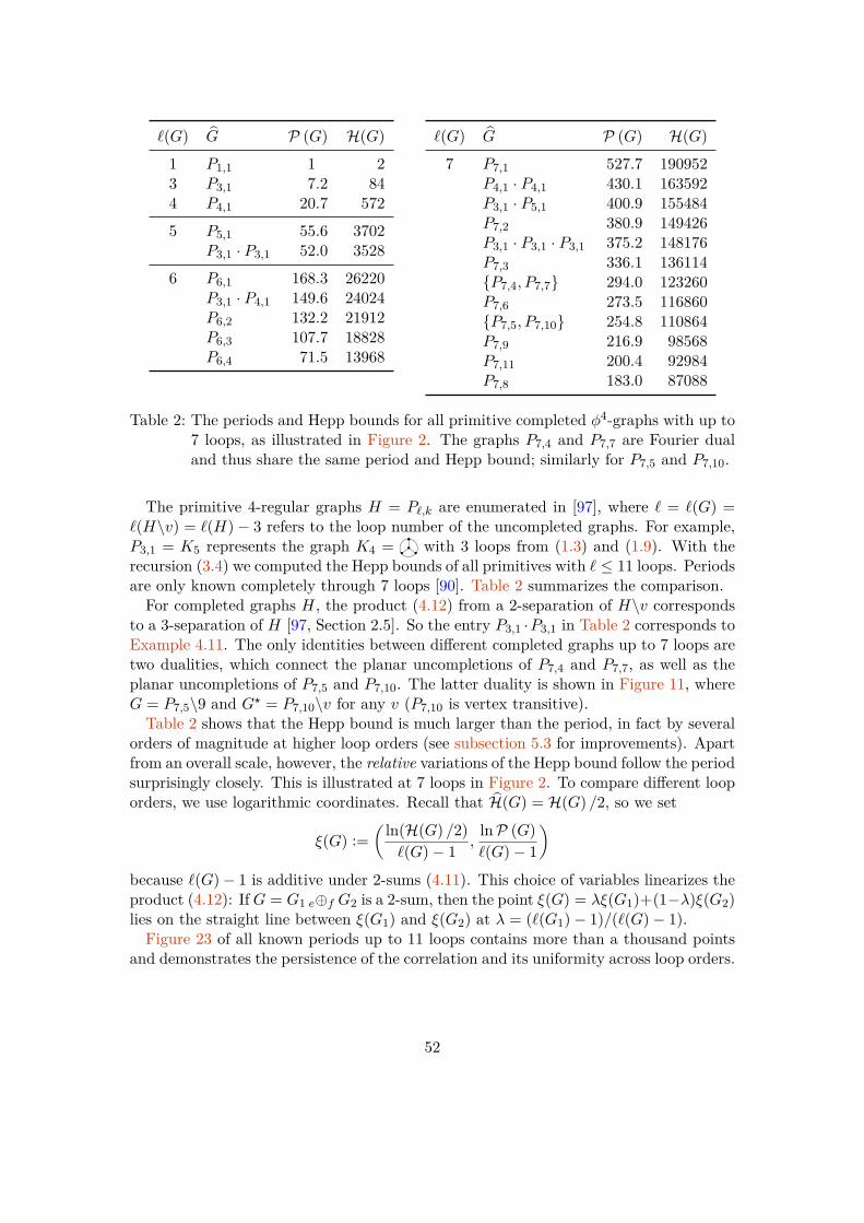
`(G) G P (G) H(G)

1 P1,1 1 23 P3,1 7.2 844 P4,1 20.7 572

5 P5,1 55.6 3702P3,1 · P3,1 52.0 3528

6 P6,1 168.3 26220P3,1 · P4,1 149.6 24024P6,2 132.2 21912P6,3 107.7 18828P6,4 71.5 13968

`(G) G P (G) H(G)

7 P7,1 527.7 190952P4,1 · P4,1 430.1 163592P3,1 · P5,1 400.9 155484P7,2 380.9 149426P3,1 · P3,1 · P3,1 375.2 148176P7,3 336.1 136114P7,4, P7,7 294.0 123260P7,6 273.5 116860P7,5, P7,10 254.8 110864P7,9 216.9 98568P7,11 200.4 92984P7,8 183.0 87088

Table 2: The periods and Hepp bounds for all primitive completed φ4-graphs with up to7 loops, as illustrated in Figure 2. The graphs P7,4 and P7,7 are Fourier dualand thus share the same period and Hepp bound; similarly for P7,5 and P7,10.

The primitive 4-regular graphs H = P`,k are enumerated in [97], where ` = `(G) =`(H\v) = `(H)− 3 refers to the loop number of the uncompleted graphs. For example,P3,1 = K5 represents the graph K4 = with 3 loops from (1.3) and (1.9). With therecursion (3.4) we computed the Hepp bounds of all primitives with ` ≤ 11 loops. Periodsare only known completely through 7 loops [90]. Table 2 summarizes the comparison.For completed graphs H, the product (4.12) from a 2-separation of H\v corresponds

to a 3-separation of H [97, Section 2.5]. So the entry P3,1 ·P3,1 in Table 2 corresponds toExample 4.11. The only identities between different completed graphs up to 7 loops aretwo dualities, which connect the planar uncompletions of P7,4 and P7,7, as well as theplanar uncompletions of P7,5 and P7,10. The latter duality is shown in Figure 11, whereG = P7,5\9 and G? = P7,10\v for any v (P7,10 is vertex transitive).Table 2 shows that the Hepp bound is much larger than the period, in fact by several

orders of magnitude at higher loop orders (see subsection 5.3 for improvements). Apartfrom an overall scale, however, the relative variations of the Hepp bound follow the periodsurprisingly closely. This is illustrated at 7 loops in Figure 2. To compare different looporders, we use logarithmic coordinates. Recall that H(G) = H(G) /2, so we set

ξ(G) :=( ln(H(G) /2)

`(G)− 1 ,lnP (G)`(G)− 1

)because `(G)− 1 is additive under 2-sums (4.11). This choice of variables linearizes theproduct (4.12): If G = G1 e⊕f G2 is a 2-sum, then the point ξ(G) = λξ(G1)+(1−λ)ξ(G2)lies on the straight line between ξ(G1) and ξ(G2) at λ = (`(G1)− 1)/(`(G)− 1).Figure 23 of all known periods up to 11 loops contains more than a thousand points

and demonstrates the persistence of the correlation and its uniformity across loop orders.

52

bb b b b

b b b b b b b b b b b b bb b

b b

b

r

r

r

r

+

++

+

+

+

+

++

+

++

+

+

+

+

++++

++

+++++

++++

+ +++

+

+ +

+

++++++++

+ +++++++++++++

+++++++++++ ++++++++

+ ++++

++

+

+

+ +++ +++++++

++++++++++++

+++++++++++++++++++++++

+++++++++++++++++++++++++++

+++++++++++++++++++++

++++++++++++++ +++++ ++

+ + ++

+

++++ + +++ +++++++

++++++++++++++++++++++++++++++++++++++++++++++++++++++++

+++++++++++++++++++++++++++++++++++++++++++++++++++++++++++++++++++++++

++++++++++++++++++++++++++++++

++++++++++++++++ +++ ++++

++

+

P3,1

P4,1P5,1

P6,1P7,1

P8,1

P9,1

P10,1

P11,1

P6,4

P6,2

P6,3

P11,2

P8,2

P8,24

P8,29

0.85

0.90

0.95

1.00

1.05

1.10

1.76 1.80 1.84 1.88 1.92 1.96

ln(H/2)ℓ−1

lnP

ℓ−1

Figure 23: φ4 periods from [90] and their Hepp bounds (products not included). Graphswith 6 and 8 loops are highlighted with orange diamonds and blue circles.

=

P8,30 P8,31 P8,35 P8,36

Figure 24: The smallest φ4 primitives with unexplained Hepp bound equalities.

Remark 5.1. Despite the strong correlation evident in Figure 2 and Figure 23, we cannotstrengthen Conjecture 1.2 to the equivalence P (G1) ≤ P (G2) ⇔ H(G1) ≤ H(G2) ofinequalities. In other words, the plots are not monotone—though one needs to zoom inclosely to notice this. For example, in [90] we find that

5548.00 ≈ P (P10,48\v) < P (P10,255\v) ≈ 5549.93, but32743060 = H(P10,48\v) > H(P10,255\v) = 32740360.

5.2 Unexplained identitiesThe first examples of equal Hepp bounds in φ4 theory that do not follow from any knownsymmetry are H(P8,30\v) = H(P8,36\v) and H(P8,31\v) = H(P8,35\v) as stated in (1.8).These four graphs are depicted in Figure 24 and structurally rather different:

graph G Aut(G) triangles ancestor uncompletions c2(G)

P8,30 Z/2Z 4 P7,11 5 −z3P8,31 Z/2Z× Z/2Z 3 P7,8 7 −z2P8,35 D8 4 P8,35 2 −z2P8,36 D5 5 P8,36 2 −z3

Both P8,30 and P8,31 have a double triangle and are thus descendants of P7,11 and P7,8,respectively, in the terminology of [97]. Their Hepp bound partners P8,35 and P8,36 have

53

` primitives = Heppbounds + Fourier

& twist + Fouriersplit + unexplained

identities7 11 = 9 + 2 + 0 + 08 41 = 29 + 10 + 0 + 29 190 = 129 + 55 + 1 + 510 1182 = 776 + 346 + 13 + 4711 8687 = 6030 + 2411 + 55 + 191

Table 3: Tally of known and unexplained identities of Hepp bounds of φ4 graphs.

no double triangles and larger, dihedral symmetry groups: P8,35 arises by attaching twovertices to the circulant C8

1,4 and P8,36 features a cyclic arrangement of five triangles.Apart from the equality of Hepp bounds, it is notable that also the c2-invariants and

the permanents coincide within both pairs of graphs. In particular the latter indicates astrong relationship of these pairs, because the permanent is a very rich invariant—exceptfor relations following from the four symmetries of [97], the permanents of two differentgraphs coincide only in very few cases [44, Appendix A].We are thus led to Conjecture 1.2, motivated by the expectation that all these identities

are not accidents but rather a consequence of some underlying combinatorial relationshipof the graphs, like the symmetries in section 4. This structure remains to be identified,but we hope that a mechanism explaining equality of Hepp bounds, permanents and c2invariants might also force the periods to be equal.All data from [90] is compatible with Conjecture 1.2 and further corroborated by

[70]. We computed the Hepp bounds for all primitive φ4 graphs with ` ≤ 11 loops, andwhenever two graphs share the same Hepp bound and their periods are known, then theperiods indeed coincide. The same holds for the known c2 invariants [70, 90] and thepermanents computed in [44]. Note that this is necessary for Conjecture 1.2 to be viable,because it is conjectured that graphs with equal period have the same c2 invariant [26,Conjecture 5] and the same permanent [45, Conjecture 1].Out of the four graphs in Figure 24, only P8,31 could be computed in [90]. The number

of unknown 8-loop φ4 periods would drop from 8 in [90] to 6 if the conjectures

P (P8,30\v) ?= P (P8,36\v) and P (P8,31\v) ?= P (P8,35\v)

were to be verified. At higher loop orders, there are many more period relations thatwould follow through Conjecture 1.2 from unexplained identities of Hepp bounds. Thesummary in Table 3 starts out with the number of irreducible primitives, i.e. completedprimitive φ4 graphs that do not have a three-vertex cut. In this setup of [97], productrelations are absent and the completion symmetry is automatically taken care of.

The number of different Hepp bounds (third column) is smaller, because differentcompletion classes can evaluate to the same Hepp bound. The bulk of these identities isexplained by the twist and Fourier relations from [97], and a few more identities followfrom the Fourier split discussed in [70]. From 8 loops onwards, there are leftover identities

54

of Hepp bounds that are not explained by any of these symmetries (last column), thefirst examples of which are (1.8).

5.3 Improved boundsThe wheel graphs W` illustrate the huge gap between the Hepp bound and the period:According to Proposition 3.19, their Hepp bounds grow by a factor of 9 per loop, whereasthe periods only gain a factor of 4 per loop [20]:

P (W`) =(

2`− 2`− 1

)ζ (2`− 3) ∼ 4`−1

√π`.

To improve the bound, we can drop the numerator |γ1| · · · |G/γ`−1| in the formula (3.2)that sums over flags γ1 ( · · · ( γ` = G of bridgeless subgraphs (see Corollary 5.6). Thisfollows from an approximation of the graph polynomial ΨG by products of one-loopgraphs, within the sector associated to the flag,

D1piγ• :=

0 < max

e∈γ1xe < max

e∈γ2/γ1xe < · · · < max

e∈G/γ`−1xe

⊂ RN

+ . (5.1)

Theorem 5.2. The period P (G) ≤ Hlog (G) is bounded by

Hlog (G) :=∑

γ•∈F1piG

c|γ1|c|γ2\γ1| · · · c|G\γ`−1|

ω(γ1) · · ·ω(γ`−1) , (5.2)

where the positive reals cn ∈ R are defined for all integers n ≥ 1 by

cn :=∫

[0,1]n

dx1 · · · dxn(x1 + · · ·+ xn)2 δ

(1− max

1≤i≤nxi

). (5.3)

Example 5.3. With Table 4, the flags of K4 from Example 3.3 give the bound

Hlog (K4) = 12c3c2c11 · 1 + 6c4c1c1

2 · 1 = 72 ln 3− 96 ln 2 ≈ 12.56.

Proof. For any subgraph γ ⊆ G, the spanning trees T ∈ TG with the property thatF = γ∩T is a spanning forest of γ are easily seen to stand in bijection with pairs (F, T ′)of spanning forests F of γ and spanning trees T ′ of the quotient G/γ [24, Proposition 2.2].Applied to a bridgeless flag γ• ∈ F1pi

G with ` = `(G) elements, this gives an injection

Tγ1 × Tγ2/γ1 × · · · × TG/γ`−1 → TG, (T1, . . . , T`) 7→ T1 ∪ · · · ∪ T`

covering precisely those spanning trees T ∈ TG such that T ∩ γk is a spanning forest ofγk, for each 1 ≤ k ≤ `. In terms of the graph polynomials, this gives the inequality

ΨG ≥ Ψγ1Ψγ2/γ1 · · ·ΨG/γ`−1 , (5.4)

55

n 1 2 3 4 5

cn 1 1 6 ln 2− 3 ln 3 36 ln 3− 56 ln 2 360 ln 2− 135 ln 3− 1252 ln 5

≈ 0.863 ≈ 0.734 ≈ 0.630

Table 4: The coefficients (5.3) that appear in the numerator of the improved bound (5.2).

which goes back to [9, Proposition 3.5] and is crucial for the desingularization of Feynmanintegrals [24, 101]. The quotients γk/γk−1 are cycles, such that Ψγk/γk−1 =

∑e∈γk\γk−1

xe,and we can therefore estimate the period integral over the flag sector (5.1) by

∫D1piγ•

ΩΨ2G

=∫D1piγ•

ΩΨ2G

∏k=1

∫ ∞0

dλk δ(λk − max

e∈γk/γk−1xe

)

≤∫

0<λ1<···<λ`=1

`−1∏k=1

λ|γk/γk−1|k

dλkλ3k

∏k=1

c|γk/γk−1|

by changing variables to xe = λkye for e ∈ γk. The iterated integral over the λk’sgenerates the product

∏`−1k=1(|γk| − 2k) =

∏`−1k=1 ω(γk) in the denominator of (5.2).

We can relabel the maximal Schwinger parameter in (5.3) to be x1, so that

cn = n

∫[0,1]n−1

dx2 · · · dxn(1 + x2 + · · ·+ xn)2 . (5.5)

For small n, these integrals are listed in Table 4. For large n, they grow asymptoticallylike cn ∼ 4/n+O(n−2), but we will not use this. From n ≥ 3, they involve logarithms,

cn = 1(n− 3)!

n∑k=2

(n

k

)(−1)k+n+1kn−2 ln k, (5.6)

which follows in the limit ρ→ −3 from the elementary integral (for non-integral ρ)

n∏e=2

∫ 1

0dxe

(1 +

n∑i=2

xi

)ρ+1

= 1(ρ+ 2) · · · (ρ+ n)

∑I⊆2,...,n

(−1)n−|I| (1 + |I|)ρ+n .

Remark 5.4. The improved boundHlog (G) does not respect any of the period symmetriesexactly. For example, the two uncompletions in Figure 1 differ slightly:

Hlog

( )= 6(c6+3c5+9c4+6c3+10c2

3+7c3c4) ≈ 156.63 6= Hlog

( )≈ 156.54.

Lemma 5.5. The sequence cn defined in (5.3) starts with c1 = c2 = 1 and is strictlydecreasing thereafter. In particular, cn ≤ 1 for all n.

56

G P (G) H(G) Hden (G)

P1,1 1 2 1P3,1 7.2 84 15P4,1 20.7 572 59

P5,1 55.6 3702 224P3,1 · P3,1 52.0 3528 216

G P (G) H(G) Hden (G)

P6,1 168.3 26220 909.5P3,1 · P4,1 149.6 24024 852P6,2 132.2 21912 795.5P6,3 107.7 18828 709.5P6,4 71.5 13968 567

Table 5: Comparison of the Hepp bound and its improvement (5.7) for ` ≤ 6 loops.

Proof. Let yi := x1 + · · ·+xi−1 +xi+1 + · · ·+xn, then the convexity of x 7→ x−2 implies(n∑i=1

xi

)−2

=(

1n− 1

n∑i=1

yi

)−2

=(n− 1n

)2(

1n

n∑i=1

yi

)−2

≤ (n− 1)2

n3

n∑i=1

1y2i

.

Now set x1 := 1 and integrate over x2, . . . , xn, then using (5.5) we find that

cn ≤(n− 1)2

n2

n∑i=1

∫[0,1]n−1

dx2 · · · dxny2i

= (n− 1)2

n2

(cn−1 + cn−1

n− 3

). (∗)

Here we exploited that each of the n − 1 summands with i > 1 just integrates to cn−1n−1 ,

whereas the first summand with i = 1 contributes the term cn−1n−3 according to (5.3) and∫

[0,1]n−1

dx2 · · · dxn(x2 + · · ·+ xn)2 =

∫ 1

0

tn−1

t2dtt

∫[0,1]n−1

dy2 · · · dyn(y2 + · · ·+ yn)2 δ

(1− max

2≤i≤nyi

),

upon changing variables to t := max2≤i≤n xi and xi = tyi. From (∗) then we see that

cncn−1

≤ 1− n2 − 5n+ 2n2(n− 3) < 1

for all n ≥ 5, and the remaining relations c4 < c3 < c2 are demonstrated in Table 4.

Corollary 5.6. The period P (G) ≤ Hden (G) is bounded by the rational number

Hden (G) :=∑

γ•∈F1piG

1ω(γ1) · · ·ω(γ`(G)−1) ∈ Q. (5.7)

This slightly bigger, but rational bound follows from (5.2) because the products of ckin the numerators are ≤ 1. For Example 3.3, Hden (K4) = 12 · 1

1·1 + 6 · 12·1 = 15 is much

closer to P (K4) ∼= 7.2 than H(K4) = 84. More comparisons are given in Table 5.In contrast toHlog (G), the rational boundHden (G) does respect completion symmetryHden (G\v) = Hden (G\w), and the same proof as for Theorem 4.21 applies. But theother symmetries fail: Duality is violated by the pair (P7,5\9)? ∼= P7,10\v from Figure 11:

Hden (P7,5\9) = 50152 6= 2517 = Hden (P7,10\v) .

57

For the twist from Figure 20, we find the values

Hden (P7,4\p) = 108554 6= 5443

2 = Hden (P7,7\p) ,

and there is no product relation between 225 = Hden (K4)2 and the 2-sum

Hden

( )= Hden

(e⊕f

)= 216.

Remark 5.7. An analogous improvement applies to the formula (3.6) expressing the Heppbound as a sum over flags of flats (induced subgraphs). The integration sector is then

Dflatγ• :=

0 < min

e∈γ1xe < min

e∈γ2/γ1xe < · · · < min

e∈M/γr−1xe

⊂ RN

+ ,

and we arrive at the improved rational bound Hflatden (G) ≥ P (G) given by

Hflatden (G) :=

∑γ•∈Fflat

G

1ω(γ1) · · ·ω(γrk(G)−1) ∈ Q.

For planar graphs, Remark 4.7 shows Hflatden (G) = Hden (G?), but otherwise the improved

bounds are unrelated. The bound Hflatden (G) violates all symmetries, even completion:

Hflatden

( )= 218 6= 216 = Hflat

den

( )= Hden

( )= Hden

( ).

Proposition 5.8. The improved Hepp bounds of the wheel graphs with n loops are

Hden (Wn) = Hflatden (Wn) = −n(n− 3)

2(n− 2) + 24n

n∑k=1

(2n− 2kn− k

)(2kk

)k · 5n−k ∼ 5n+1/2

8√πn

.

Proof. Note that W ?n = Wn is self-dual. For the improved bound Hflat

den (Wn), the numer-ator a?M/γ disappears from the recursion (3.11). With this modification, the calculationas in the proof of Proposition 3.19 produces the generating function

∞∑n=3Hden (Wn) zn = z3(z − 2)

2(1− z)2 − 4z2 log(1− z) + z√(1− 5z)(1− z)3 .

The numerator |γ1| · · · |G/γ`−1| in the flag formula (3.2) is at most 2`, because thefactors add to |EG| = 2`. The improved bound is therefore at least Hden (G) ≥ H(G) /2`,so the gain of 5/9 per loop in the ratio Hden (Wn) /H(Wn) is almost as good as possible.

Up to the overall scale, the improved bounds show a very similar correlation as inFigure 23 (see Table 5). The most notable difference is that a single period branches intoseveral data points with slightly different abscissa, due to the violation of symmetries.

58

6 Polyhedral geometryIn the spirit of tropical geometry, let us change variables from the Schwinger parametersxi = e−yi to their logarithms yi = − log xi. Then

∏i/∈T xi = exp (−~y ·~eT c) in terms of

the characteristic vector ~eT c =∑i/∈T ~ei ∈ RN of the complement T c of any spanning

tree T . In the affine chart x1 = 1, the Hepp bound integrand from (1.13) then becomes

Ω(~a)(Ψtr

G)d/2

∣∣∣∣∣x1=1

= exp[−~y · ~a− d

2 maxT∈TG

(−~y ·~eT c)]y1=0

dy2 · · · dyN .

Definition 6.1. The exponent defines a continuous, piecewise linear function

RN 3 ~y 7→ ω~a(~y) := ~y · ~a+ d

2 maxT∈TG

(−~y ·~eT c) (6.1)

where, as always, d2 = a1+···+aN

`(G) is fixed by the constraint ω~a(G) = 0.2 In particular,locally this function is a homogeneous bilinear form in ~y and ~a.

Corollary 6.2. The Hepp bound integral (1.13) can be written as3

H(G,~a) =∫RN

e−ω~a(~y)δ(yi)dN~y. (6.2)

As the notation suggests, Definition 6.1 generalizes the superficial degree of conver-gence (2.3): For the characteristic vector ~eγ =

∑i∈γ ~ei of a subgraph γ ⊆ G, we observe

−~eγ ·~eT c = |γ ∩ T | − |γ| = κ(γ)− κ(γ ∩ T )− `(γ)

by (2.2) and `(γ∩T ) = 0. Here we consider both γ and γ∩T as graphs on the same set ofvertices, so the number of connected components κ(γ∩T ) is at least κ(γ). Consequently,

ω~a(~eγ) = ~eγ · ~a−d

2`(γ) + maxT∈TG

(κ(γ)− κ(γ ∩ T )) = ω~a(γ) (6.3)

indeed coincides with (2.3) and the maximum is attained precisely on all those trees Tfor which T ∩ γ is a spanning forest of γ. Assuming d > 0, (6.1) is a maximum of linearforms, and hence ω~a(~y) is a convex function of ~y. It describes two convex polyhedra [68]:

Definition 6.3. We define the Newton polytope NG(~a) and its polar N G(~a) as

NG(~a) := ~a− d2 conv ~eT c : T ∈ TG ⊂ RN and (6.4)

N G(~a) :=⋂

T∈TG

~y : ~y ·

(~a− d

2~eT c)≤ 1

⊂ RN , (6.5)

where conv ~v1, . . . , ~vn = ∑ni=1 λi~vi :

∑ni=1 λi = 1 and all λi ≥ 0 is the convex hull.

We abbreviate the case of unit indices as NG := NG(1, . . . , 1) and N G := N G(1, . . . , 1).

59

N (1, 1)

−1

1

1 2−1−2

y1

y2

b

b

N (1, 1)

N

(

3

2,1

2

)

−1

1

1 2−1−2

y1

y2

b

b

N

(

3

2,1

2

)

Figure 25: The Newton polytope (line segment) and its polar (shaded unbounded region)for the bubble graph C2 = . The figure to the left shows unit indicesa1 = a2 = 1, the other depicts ~a = (1.5, 0.5).

Remark 6.4. Every vector ~a − d2~eT c is a vertex of NG(~a) and lies in the hyperplane

orthogonal to the diagonal vector ~1 := (1, . . . , 1) = ~eG, because ~1 · ~eT c = `(G) asdiscussed above and ~1 ·~a− d

2`(G) = ω(G) = 0. Hence the dimension of NG(~a) is at mostN − 1. It also implies that the function (6.1) is invariant under translations by ~1, thatis ω~a(~y + λ~1) = ω~a(~y) for all real λ. Hence N G(~a) contains the line R ·~1. In summary,

NG(~a) ⊂~y : ~y ·~1 = 0

⊂ RN and (6.6)

N G(~a) = N G(~a) +R ·~1. (6.7)

Example 6.5. The cycle CN with N edges 1, . . . , N has one spanning tree T = CN \ ifor each edge i, which contributes the monomial xi to ΨCN =

∑Ni=1 xi. Hence

NCN (~a) = ~a− (a1 + . . .+ aN ) conv ~ei : 1 ≤ i ≤ N

is an affine image of the standard simplex. For the bubble C2 = it is the line segment

N (a1, a2) = conv( a1−a1 ),

(−a2a2

)=(

λ−λ

): −a2 ≤ λ ≤ a1

⊂ R2

illustrated in Figure 25. Its polar is the unbounded region

N (a1, a2) =~y : − 1

a2≤ y1 − y2 ≤ 1

a1

⊂ R2.

The terminology in Definition 6.3 reflects that the convex hull conv ~eT c : T ∈ TG ofthe exponents of the monomials in ΨG is called the Newton polytope of ΨG. Note thatNG(~a) is just the translate by ~a of this polytope, after scaling it by −d

2 . Similarly we canthink of an affine transformation of the polytope conv ~eT : T ∈ TG, which is called thespanning tree polytope [34] of G or more generally the matroid polytope [60] of M(G).Indeed, the entire discussion in this section extends to arbitrary matroids by replacingthe spanning trees TG = BM(G) with the bases BM throughout.

2In the (uninteresting) case `(G) = |T c| = 0, we get ~eTc = 0 and thus ω~a(~y) = ~y · ~a.3Instead of yi = 0, we can restrict to an arbitrary hyperplane ~y · ~ν = 0 as long as ν1 + . . .+νN = 1.

60

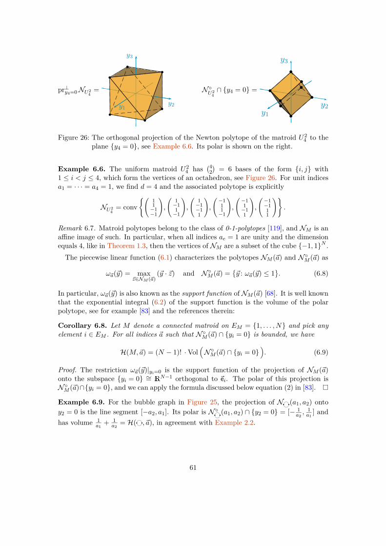
pr⊥y4=0NU24

=

bb

bb

b

b

y1y2

y3

N U2

4∩ y4 = 0 =

b

bb

b

b

bb

by1

y2

y3

Figure 26: The orthogonal projection of the Newton polytope of the matroid U24 to the

plane y4 = 0, see Example 6.6. Its polar is shown on the right.

Example 6.6. The uniform matroid U24 has

(42)

= 6 bases of the form i, j with1 ≤ i < j ≤ 4, which form the vertices of an octahedron, see Figure 26. For unit indicesa1 = · · · = a4 = 1, we find d = 4 and the associated polytope is explicitly

NU24

= conv(

11−1−1

),

(1−11−1

),

(1−1−11

),

(−111−1

),

(−11−11

),

(−1−111

).

Remark 6.7. Matroid polytopes belong to the class of 0-1-polytopes [119], and NM is anaffine image of such. In particular, when all indices ae = 1 are unity and the dimensionequals 4, like in Theorem 1.3, then the vertices of NM are a subset of the cube −1, 1N .

The piecewise linear function (6.1) characterizes the polytopes NM (~a) and N M (~a) as

ω~a(~y) = max~z∈NM (~a)

(~y · ~z) and N M (~a) =~y : ω~a(~y) ≤ 1

. (6.8)

In particular, ω~a(~y) is also known as the support function of NM (~a) [68]. It is well knownthat the exponential integral (6.2) of the support function is the volume of the polarpolytope, see for example [83] and the references therein:

Corollary 6.8. Let M denote a connected matroid on EM = 1, . . . , N and pick anyelement i ∈ EM . For all indices ~a such that N M (~a) ∩ yi = 0 is bounded, we have

H(M,~a) = (N − 1)! ·Vol(N M (~a) ∩ yi = 0

). (6.9)

Proof. The restriction ω~a(~y)|yi=0 is the support function of the projection of NM (~a)onto the subspace yi = 0 ∼= RN−1 orthogonal to ~ei. The polar of this projection isN M (~a)∩yi = 0, and we can apply the formula discussed below equation (2) in [83].

Example 6.9. For the bubble graph in Figure 25, the projection of N (a1, a2) ontoy2 = 0 is the line segment [−a2, a1]. Its polar is N (a1, a2) ∩ y2 = 0 = [− 1

a2, 1a1

] andhas volume 1

a1+ 1

a2= H( ,~a), in agreement with Example 2.2.

61

We learn that the Hepp bound integrals (1.13) and (6.2) converge precisely when thepolyhedron N M (~a) ∩ yi = 0 is bounded. Equivalently, the orthogonal projection ofNM (~a) onto yi = 0 ∼= RN−1 must contain the origin in its interior. This requires thatthe dimension of NM ⊂ ~y ·~1 = 0 ⊂ RN is N − 1 (as big as possible).

Lemma 6.10 ([62, Corollary 3.10] and [60, Proposition 2.4]). For a matroid M onEM = 1, . . . , N, the dimension of the polytope NM (~a) ⊂ RN is equal to N − κ(M).

For a disconnected matroid, the polar is thus never bounded. But if M is connected,then the projection ofNM onto yi = 0 has full dimensionN−1. In this case, there existtranslations ~a which put the origin inside, and then the polar is bounded. Explicitly, wesee that ~0 ∈ NM (~a) precisely when ~a ∈ d

2 conv ~eT c : T ∈ BM, according to (6.4).

Corollary 6.11. For a connected matroid M , the domain Θ ⊂ RN of absolute conver-gence of the integrals (1.13) and (6.2) is not empty. It is the interior of the cone

Θ = R≥0 · conv ~eT c : T ∈ BM .

It follows that the definitions of the Hepp bound by integrals (1.13) and (6.2), flags(2.4) and volumes (6.9) are completely equivalent:

1. If M is connected, then inside the region Θ, the integral is finite and equal to thepolar volume and the Hepp bound. This local information fixes the Hepp bounduniquely as a rational function by analytic continuation.

2. If M is not connected, the polar volume and the integral do not converge for anyindices ~a, and the combinatorial formula gives zero.

6.1 Singularities, facets and verticesThe geometry explains the origin of the singularities of the Hepp bound. First, recallthat every vertex ~v = ~a− d

2~eT c of the Newton polytope NM (~a) lies in the half-spaces

hγ := ~y : ~eγ · ~y ≤ ω~a(γ) ⊂ RN

associated to every non-empty subset γ (M , due to ~eγ ·~v = ω~a(γ)− (κ(γ∩T )−κ(γ)) ≤ω~a(γ) from (6.3). Consequently, the Newton polytope is contained in the intersection ofall these half-spaces. The boundary hyperplanes ∂hγ slice off the faces

Fγ := NM (~a) ∩ ~y : ~eγ · ~y = ω~a(γ)

from NM (~a). When ~a approaches the boundary ∂Θ ⊂⋃γ ~a : ω~a(γ) = 0 of the con-

vergence cone, then the origin lands on some such face Fγ so that the projected polarbecomes unbounded.The poles of the Hepp bound are therefore in bijection with the facets (faces of codi-

mension one) of Θ =⋂γ ω(γ) ≥ 0 andNM (~a). Hence Corollary 2.38 describes precisely

those submatroids γ ⊂ M for which the hyperplanes ~y : ω(γ) = 0 and ∂hγ supportfacets of Θ and NM (~a), respectively. This gives an alternative derivation of the well-known facet description of matroid polytopes:

62

Lemma 6.12 ([60, Proposition 2.6] and [62, Corollary 3.14]). Given a connected matroidM , the facets of the polytope NM are in bijection with the submatroids ∅ 6= γ (M suchthat γ and the quotient M/γ are both connected.

We denote these submatroids in (2.19) as SM . The Newton polytope is therefore

NM (~a) =⋂

γ∈SM

~y : ~eγ · ~y ≤ ω~a(γ) ∩~y : ~1 · ~y = 0

(6.10)

and none of these constraints is redundant. From these facets we read off the vertices ofthe polar, making the divergences of the Hepp bound on ω~a(γ)→ 0 for γ ∈ SM apparent:

Corollary 6.13. The polar of the Newton polytope of a connected matroid M is

N M (~a) = R ·~1 + conv

~eγω~a(γ) : γ ∈ SM

, (6.11)

and no γ ∈ SM is redundant. Each such γ labels a vertex of the intersection

N M (~a) ∩ yi = 0 = conv(

~eγω~a(γ) : i /∈ γ ∈ SM

∪ −~eγcω~a(γ) : i ∈ γ ∈ SM

). (6.12)

Example 6.14. The uniform matroid U24 has precisely 8 singular submatroids γ ∈ SU2

4:

the singletons e and their complements (Example 2.39). For unit indices, they all haveω(γ) = 1 and we can read off the vertices of the polar in Figure 26 directly from (6.12):

N U24∩ y4 = 0 = conv

( 100

)1

,( 0

10

)2

,( 0

01

)3

,(−1−1−1

)4

,(−1

00

)2,3,4

,( 0−10

)1,3,4

,( 0

0−1

)1,2,4

,( 1

11

)1,2,3

.

(←γ)

This rhombohedron extends the cross-polytope conv ±~e1,±~e2,±~e3 with volume 4/3by two tetrahedra ± conv ~e1,~e2,~e3,~e1 +~e2 +~e3 which each have volume 1/3. So thetotal volume is 2 and we find H

(U2

4)

= 3! · 2 = 12 from (6.9) in agreement with (2.9).

Remark 6.15. The Newton polytope differs from the Feynman polytope defined in [24],which has many more facets. They are labelled by all ‘motic’ (bridgeless) subgraphs ofthe given graph G, whereas only very few of those belong to SG.

6.2 FactorizationThe facet Fγ defined above for a submatroid γ ∈ SM contains precisely those vertices~v = ~a− d

2~eT c of NM (~a) such that γ ∩T is a basis of γ, see (6.3). In this case we see thatT \ γ is a basis of M/γ, and hence the vertices of Fγ are in bijection with the Cartesianproduct Bγ × BM/γ . The corresponding factorization

∂NM (~a) ⊃ Fγ ∼= Nγ ×NM/γ (6.13)

is the geometric incarnation of the algebraic relation ΨM ≡ ΨγΨG/γ mod I, where I isthe ideal generated by monomials of degree `(γ) + 1 in the variables ae : e ∈ γ. We

63

G P7,4\r P7,4\q P7,4\t P7,4\p P7,4\s

|TG| 1137 1166 1168 1197 1248|SG| 66 64 69 69 81

P7,4 =

p

q t

r s

Table 6: Facet and vertex counts of N G for different uncompletions of the graph P7,4.

exploited this relation in (5.4), and it is absolutely fundamental in the study of Feynmanamplitudes and graph polynomials [9, 24, 25, 101].Regarding the Hepp bound, we see from (6.11) that the divergence at ω~a(γ) → 0

comes from a pyramid with the runaway apex ~eγ/ω~a(γ). Its volume comes from thepiece of the integral (6.2) where ~y ranges over the cone R>0Fγ . The factorization (6.13)thus leads to a product formula for the residue, namely (2.17).

6.3 ComputationsThe calculation of the volume of a convex polytope is a difficult, but very well studiedproblem. In small dimensions, we can resort to exact algorithms like lrs [5]. We testedthis program on all φ4 periods with at most 7 loops. Taking the vertex description (6.12)as input, lrs determines the facets and computes the volume. In all cases, these facetsmatch precisely the spanning trees according to (6.5), and the volume reproduces theHepp bound computed by (3.2) in line with (6.9). We found cddr+ [63] to be moreefficient for the transformation between facets and vertices, but it does not provide avolume computation.Such exact volume determinations are very time consuming and in our tests only

practical up to around 15 dimensions (graphs with 16 edges). Not surprisingly, a directcombinatorial recursion like (3.4) is much more efficient. Our implementation of thismethod succeeded for graphs with 30 edges. The Hepp bound thus provides a datasetof polytopes in a large number of dimensions with exactly known volumes, which mightbe useful as a benchmark for general volume computation algorithms.We are not aware of previous work on the polar volume of matroids, but the volume

of the matroid polytope itself has been studied in the literature. For example, a combi-natorial formula was given in [2] using the theory of generalized permutohedra [92]. Forfixed rank or corank, the volume of a matroid polytope can be computed in polynomialtime [49]. Our Corollary 3.10 is the same statement about the volume of the polar.Recently it has become feasible to approximate volumes of polytopes in very high

dimension, using rapidly mixing random walks. At least three implementations of suchmethods are readily available [38, 59, 64]. These techniques open up the fascinatingpossibility to study properties of very large graphs and matroids, which might giveinsights into the asymptotic behaviour of the perturbation series of quantum field theory.Remark 6.16. Completion invariance identifies the volumes of combinatorially distinctpolytopes. The graph from [97] in Table 6 has five non-isomorphic uncompletions G =P7,4\v and each of them has a different number of spanning trees (facets of N G). Table 6

64

also shows the number of divergent subgraphs (vertices of N G). By Theorem 4.21, thevolumes 13! ·Vol(N G∩yi = 0) = H(G) = 123260 of these five different polar polytopesare all the same. The volumes of the Newton polytopes NG, however, are all distinct.In contrast, the duality (4.7) amounts to a simple reflection: N G? = −N G.

6.4 ShapeWe saw in Example 2.39 that uniform matroids U rn have only 2n vertices and hugenumber of bases, namely

(nr

). Their polars N Urn are similar to the cross-polytopes

conv ±~e1, . . . ,±~en, which also have 2n vertices, and the maximal number 2n of facets.For p-log graphsG in 4 dimensions (n = |G| = 2`), like the φ4 graphs considered above,

we find experimentally a roughly similar behaviour. The number of spanning trees growsexponentially with n; this follows from [85]. Therefore, N G has an exponentially largenumber of facets. The number |SG| of vertices of N G, in contrast, appears to grow veryslowly in comparison. For the zigzag graphs from [22], for example, one can show that|SG| is quadratic in n.The similarity between N G and the cross-polytope is particularly pertinent in regards

of the volumes. We see from (6.5) that ±~ek ∈ N G for all 1 ≤ k ≤ n. These correspondto single edge subgraphs and their complements. It follows that N G ∩yn = 0 containsthe cross-polytope of dimension n− 1 = 2`− 1, which implies the lower bound

H(G) ≥ (n− 1)! ·Vol (conv ±~e1, . . . ,±~en−1) = 2n−1. (6.14)

In fact, we get a slightly better lower bound H(U `2`) according to Remark 2.14. However,the important point to note is that H(G) grows at least exponentially with n.

Note that N G has an insphere of radius 1/√n: The vectors ~vT := ~eT −~eT c ∈ −1, 1n

solve ω(~vT /n) = 1 by (6.5) and they have norm ‖~vT ‖ =√n. The volume of this sphere

grows like (1/√n)n/Γ(1 + n/2) ∼ 1/n! for large n, up to exponential factors. With the

prefactor (n−1)! in (6.9), we see that the volume of the cross-polytope and the insphereare of comparable magnitude.The Hepp bound could however be much larger than (6.14). Since the vertices ±~ek

have distance 1 from the origin, the circumsphere of N G has radius 1 and thus its volumeexceeds that of the insphere by a factor of (

√n)n ∼

√n!.

It was proven in [48] that the periods of φ4 graphs grow only exponentially, and by(1.6) this implies an exponential upper bound on H(G) as well. We conclude that thevolume of N G is concentrated near the insphere.Remark 6.17. The polytopes NG are typically not simple and far from simplicial. A facetFγ = NG ∩ ~y : ~eγ · ~y = ω(γ) corresponding to a singular subgraph γ ∈ SG is boundedby |Tγ | · |TG/γ | vertices, and a vertex ~vT belongs to all facets Fγ such that γ ∩T spans γ.

Example 6.18. The complete graph K4 has 16 singular subgraphs: 6 singletons e,their complements K4\e ∼= , and four triangles ∼= . The vertex ~vT of NK4 corre-sponding to a star T ∼= lies on 9 facets: the three edges e ∈ T , the complements K4\fof the three edges f /∈ T , and 3 of the triangles. In the case of a path T ∼= , the vertex~vT lies on 8 facets, because it only supports 2 triangles. Conversely, the 4-dimensional

65

facets Fγ have 9 vertices if γ ∼= ; in this case, Fγ ∼= N ×N is a product of simplices.The other facets Fe ∼= N and FK4\e

∼= N have 8 vertices each.

6.5 Tree decompositionThe facets of the polar N G are in bijection with the spanning trees T of the graph G,according to (6.5). For unit indices in 4 dimensions, these facets are concretely

FT := N G ∩ ~y : ~y · (~eT −~eT c) = 1 .

They induce a decomposition N G =⋃T∈TG conv(~0 ∪ FT ) into pyramids with disjoint

interiors. The volume of such a pyramid corresponds in (6.2) to the integral over theregion where ω(~y) = ~y · (~eT −~eT c). In Schwinger parameters (1.13), this is the sector

DT :=~x :

∏e/∈T

xe >∏e/∈T ′

xe for all T ′ ∈ TG

=⋃

σ : Tσ=TDσ (6.15)

where the maximum monomial ΨtrG(~x) =

∏e/∈T xe is given by T . Each DT subsumes many

Hepp sectors Dσ as determined by Lemma 2.8. The pyramid decomposition correspondsthus to the partition

⋃T∈TG DT of the integration domain in (1.13), such that

H(G) =∑T∈TG

H(T ⊂ G) where H(T ⊂ G) :=∫DT

Ω∏e/∈T x

2e

. (6.16)

Lemma 6.19. Given a spanning tree T ∈ TG and an edge e /∈ T , let P eT ⊆ T denote theunique path in T that connects the endpoints of e. Then T ’s contribution to H(G) is

H(T ⊂ G) =∫PT

Ω∏e/∈T max xk : k ∈ P eT

. (6.17)

Proof. From Kruskal’s greedy algorithm (Lemma 2.8), we see that

DT =~x : xe > max xk : k ∈ P eT for all e /∈ T

.

The integrals of dxe/x2e over all e /∈ T therefore yield the claim.

Example 6.20. Consider the star T = 2, 4, 6 = ⊂ in G = K4 with the labelsof Figure 16. Each edge e /∈ T is connected in T by two edges: P 1

T = 2, 6, P 3T = 2, 4

and P 5T = 4, 6. The corresponding projective integral

H(

⊂)

=∫PT

Ωmax x2, x4max x2, x6max x4, x6

= 6

is easily evaluated by setting 1 = max x2, x4, x6 to obtain 6 times the affine integral∫0<x2<x4<x6=1 1/x4 = 1. For the path T = 2, 4, 5 = we find P 6

T = 4, 5 and notethat P 1

T = T has three edges. Therefore, the projective integral is smaller and we find

H(

⊂)

=∫PT

Ωmax x2, x4max x2, x4, x5max x4, x5

= 5.

As K4 has 4 stars and 12 paths as spanning trees, its Hepp bound is 4 · 6 + 12 · 5 = 84.

66

Remark 6.21. The contribution H(T ⊂ G) depends not only on T , but also on G andon the embedding of T into G. It is possible, however, to give an intrinsic upper boundon H(T ⊂ G) that only depends on T . Such a bound is constructed in [48, Appendix B]and shown to grow only exponentially with the size of the tree.Remark 6.22. Tree contributions (6.17) to the Hepp bound are not to be confused withconstructive tree weights w(G,T ) considered in [93]. The latter sum to 1 and count thefraction of Hepp sectors Dσ where T = Tσ gives the maximal monomial

∏e/∈T xe of ΨG.

These weights also have an integral representation [93, Theorem 2.1]

w(G,T ) =(∏i∈T

∫ 1

0dxi

) ∏e/∈T

min xk : k ∈ P eT ,

but in Example 6.20 this results in w(K4, ) = 1/15 and w(K4, ) = 11/180.

6.6 Period correlationFor p-log graphs with unit indices in d = 4 dimensions, the support function (6.1) is

ω(~y) = maxT∈TG

~y ·~vT where ~vT := ~eT −~eT c =∑k∈T

~ek −∑k/∈T

~ek. (6.18)

Integrating over the norm λ := ‖~y‖ in (6.2) gives∫∞

0 λN−2e−λωdλ = (N − 2)!/ωN−1, so

H(G) = (N − 2)!∫SN−1∩yi=0

Ωω(~y)N−1 (6.19)

is an integral over the N − 2 dimensional sphere SN−1 ∩ yi = 0 ∼= SN−2. The periodhas a very similar representation that explains the correlation.

Lemma 6.23. The period of a p-log graph G with N edges in 4 dimensions is equal to

P (G) = (N − 2)!∫SN−1∩yi=0

Ωω(~y)N−1 ρ(~y), (6.20)

where ρ(~y) = ρ(λ~y) for all λ > 0 takes values between 1/ |TG|2 and 1, and is defined by

ρ(~y) :=∫ ∞

0

λN−2

(N − 2)!

∑T∈TG

exp(λ

2~y ·~vTω(~y)

)−2dλ. (6.21)

Proof. Substitute xk = exp(−λyk/ω(~y)) into (2.1), this gives (6.20). For the lower boundon ρ(~y), note that the exponents are at most λ/2, because ~y ·~vT ≤ ω(~y) by (6.18), so

ρ(~y) ≥∫ ∞

0

λN−2

(N − 2)! |TG| exp (λ/2)−2 = |TG|−2 .

Furthermore, the spanning tree T that dominates for a given value of ~y contributes asummand with ~y ·~vT = ω(~y), which gives the upper bound ρ(~y) ≤ 1.

67

By comparison with (6.19), the bounds 1/ |TG|2 ≤ ρ(~y) ≤ 1 imply the relations (1.6).The corresponding lower bound P (G) ≥ 2N−1/ |TG|2 from (6.14) can be improved easily:

Lemma 6.24. The period of a p-log graph in d = 4 is at least P (G) ≥ 4N−1/ |TG|2.

Proof. Contraction and deletion of an edge show that ΨG = x1ΨG\1 + ΨG/1. Therefore,∫ ∞0

dx1Ψ2G

= 1ΨG\1ΨG/1

≥ 4(ΨG\1 + ΨG/1)2 = 4

Ψ2G|x1=1

by the arithmetic-geometric mean inequality. Repeating this estimate for the remainingedges 2, . . . , N−1 and setting xN = 1 proves the claim, since ΨG|x1=···=xN=1 = |TG|.

As discussed in subsection 6.4, the exponential upper bound on periods (and henceon the Hepp bounds) from [48] implies that the integral (6.19) is dominated by thecontributions from regions where ω(~y) is large, that is, where ~y is close to one of thespanning tree directions ~vT .Within a tree sector DT , the function ω(~y) = ~y ·~vT is linear. Together with the well-

known log-concavity of matroid polynomials [1, 86], it can be shown that the functionρ(~y) is also log-concave within each tree sector. Consequently, it is minimized at thevertices (6.11) of the polar N G:

P (G)H(G) ≥ min

γ∈SGρ(~eγ/ω(γ)).

More importantly, the log-concavity implies that ρ(~y) has a unique maximum in eachtree sector; far away from the vertices and thus closer to the centre ~vT of the correspond-ing facet of N G. As explained above, this region dominates the integral (6.19).

The arguments above give an intuition and qualitative explanation for the correlationbetween H(G) and P (G). Developing these ideas further, it should be possible to givea rigorous quantitative formulation and proof of the correlations observed in Figure 23.

7 OutlookWe explored the first properties of the Hepp bound and illustrated its rich structure,connecting algebraic, combinatorial and geometric aspects. Many interesting questionsremain, including:

1. What is the reason behind the unexplained relations like (1.8)? Are the corre-sponding periods identical as predicted by Conjecture 1.2?

2. Which p-log matroids maximize the Hepp bound? In line with [28, Conjecture 1],we conjecture that the zig-zag graphs give the largest Hepp bounds among primitiveφ4 graphs. What are the maximizers in other classes of graphs and matroids?

3. What is the computational complexity of the Hepp bound? Many techniques havebeen proposed to compute matroid polytope volumes, see for example [113]; canthese be applied to compute also the polar volumes more efficiently?

68

4. How can one prove the strong correlation between the period and the Hepp bound?Can it be improved to provide even better approximations for periods?

5. How can one extract other matroid invariants from H(M,~a) as in subsection 2.7?

The Hepp bound H(M) with unit indices is not defined when M has a divergent sub-matroid γ ( M such that |γ| /`(γ) = |M | /`(M). This can be remedied as follows: Liftthe restriction to ω(M) = 0, and consider instead the dimension d as a free parameter.Then extend the summands in (2.4) by the missing Nth denominator, and

fd(M) =∑σ∈SM

1ω(Mσ

1 ) · · ·ω(MσN ) ∈ Q(d)

is a well-defined rational function of d, with poles of the form d = 2 |γ| /`(γ). The residueat ω(M) = 0 would be the Hepp bound, were it not for the higher order of that pole dueto the presence of a divergence. Note that fd(M) = χ(Φ(M)) in terms of the map Φ(M)defined in subsection 2.7. In fact, Φ(M) is a multiplicative map of Hopf algebras, andwith (2.12), also fd(M) is multiplicative. See [39, 96] for the Hopf algebra of matroids.

The standard Hopf-algebraic renormalization techniques [25, 36] can therefore be ap-plied, and one obtains a renormalized character f+

d (M) without a pole in the dimensionof choice. One also obtains a counterterm f−d (M), which is subject to renormalizationgroup exponentiation [37]. The Hepp bound may then be defined as the correspondingcontribution to the beta function. These analogies lead to a variant of perturbativequantum field theory where all Feynman integrals can be computed in rational terms.This theory will be explored in detail elsewhere.The Hepp–period correlation may provide a new route to numerical approximations

of more general Feynman integrals with kinematic dependence.

References[1] N. Anari, S. Oveis Gharan and C. Vinzant, Log-concave polynomials, entropy,

and a deterministic approximation algorithm for counting bases of matroids, in2018 IEEE 59th Annual Symposium on Foundations of Computer Science (FOCS),pp. 35–46, IEEE, Oct., 2018. arXiv:1807.00929 [cs.DS].

[2] F. Ardila, C. Benedetti and J. Doker, Matroid polytopes and their volumes, Dis-crete & Computational Geometry 43 (2010), no. 4 pp. 841–854, arXiv:0810.3947[math.CO].

[3] N. Arkani-Hamed, Y. Bai and T. Lam, Positive geometries and canonical forms,JHEP 2017 (Nov., 2017) p. 39, arXiv:1703.04541 [hep-th].

[4] N. Arkani-Hamed, J. L. Bourjaily, F. Cachazo, A. Postnikov and J. Trnka, On-shell structures of MHV amplitudes beyond the planar limit, JHEP 2015 (June,2015) p. 179, arXiv:1412.8475 [hep-th].

69

[5] D. Avis, A revised implementation of the reverse search vertex enumeration al-gorithm, in Polytopes—Combinatorics and Computation (G. Kalai and G. M.Ziegler, eds.), pp. 177–198. Birkhäuser, Basel, 2000. program website: http://cgm.cs.mcgill.ca/~avis/C/lrs.html.

[6] C. Bergbauer, R. Brunetti and D. Kreimer, “Renormalization and resolution ofsingularities.” preprint, 2009, arXiv:0908.0633 [hep-th].

[7] M. C. Bergère, C. de Calan and A. P. C. Malbouisson, A theorem on asymptoticexpansion of Feynman amplitudes, Commun. Math. Phys. 62 (1978) pp. 137–158.

[8] M. Berghoff, Wonderful compactifications in quantum field theory, Commun. Num.Theor. Phys. 9 (2015), no. 3 pp. 477–547, arXiv:1411.5583 [math-ph].

[9] S. Bloch, H. Esnault and D. Kreimer, On motives associated to graph polynomials,Commun. Math. Phys. 267 (2006), no. 1 pp. 181–225, arXiv:math/0510011.

[10] S. Bloch and D. Kreimer, Mixed Hodge structures and renormalization in physics,Commun. Number Theory Phys. 2 (2008), no. 4 pp. 637–718, arXiv:0804.4399[hep-th].

[11] C. Bogner and S. Weinzierl, Resolution of singularities for multi-loop integrals,Comput. Phys. Commun. 178 (2008) pp. 596–610, arXiv:0709.4092 [hep-ph].

[12] C. Bogner and S. Weinzierl, Feynman graph polynomials, Int. J. Mod. Phys. A 25(2010) pp. 2585–2618, arXiv:1002.3458 [hep-ph].

[13] J. E. Bonin and A. de Mier, The lattice of cyclic flats of a matroid, Annals ofCombinatorics 12 (July, 2008) pp. 155–170, arXiv:math/0505689 [math.CO].

[14] J. E. Bonin and J. P. S. Kung, The G-invariant and catenary data of a matroid,Adv. Appl. Math. 94 (2018) pp. 39–70, arXiv:1510.00682 [math.CO]. Special issueon the Tutte polynomial.

[15] M. Borinsky, Graphs in Perturbation Theory: Algebraic Structure and Asymp-totics. Springer Theses. Springer International Publishing, 2018.

[16] A. V. Borovik, I. M. Gelfand, A. Vince and N. White, The lattice of flats and itsunderlying flag matroid polytope, Annals of Combinatorics 1 (Dec., 1997) pp. 17–26.

[17] M. Borowiecki, On hamiltonian matroids, in Graph Theory (M. Borowiecki, J. W.Kennedy and M. M. Sysło, eds.), vol. 1018 of Lecture Notes in Mathematics,(Berlin, Heidelberg), pp. 23–27, Springer, 1983. Proceedings of a Conference heldin Łagów, Poland, February 10–13, 1981.

[18] S. Borowka, G. Heinrich, S. P. Jones, M. Kerner, J. Schlenk and T. Zirke, SecDec-3.0: numerical evaluation of multi-scale integrals beyond one loop, Comput. Phys.Commun. 196 (2015) pp. 470–491, arXiv:1502.06595 [hep-ph].

70

[19] R. Britto, F. Cachazo, B. Feng and E. Witten, Direct proof of the tree-level scatter-ing amplitude recursion relation in Yang-Mills theory, Phys. Rev. Lett. 94 (May,2005) p. 181602, arXiv:hep-th/0501052.

[20] D. J. Broadhurst, Evaluation of a class of Feynman diagrams for all numbers ofloops and dimensions, Physics Letters B 164 (1985), no. 4–6 pp. 356–360.

[21] D. J. Broadhurst, Massless scalar Feynman diagrams: five loops and beyond, Tech.Rep. OUT-4102-18, Open University, Milton Keynes, Dec., 1985, arXiv:1604.08027[hep-th].

[22] D. J. Broadhurst and D. Kreimer, Knots and numbers in φ4 theory to 7 loops andbeyond, Int. J. Mod. Phys. C 6 (Aug., 1995) pp. 519–524, arXiv:hep-ph/9504352.

[23] F. C. S. Brown, “On the periods of some Feynman integrals.” preprint, Oct., 2009,arXiv:0910.0114 [math.AG].

[24] F. C. S. Brown, Feynman amplitudes, coaction principle, and cosmic Galois group,Commun. Number Theory Phys. 11 (2017), no. 3 pp. 453–556, arXiv:1512.06409[math-ph]. based on lectures (links: 1, 2, 3 and 4), given at the IHÉS in May 2015.

[25] F. C. S. Brown and D. Kreimer, Angles, scales and parametric renormalization,Lett. Math. Phys. 103 (2013), no. 9 pp. 933–1007, arXiv:1112.1180 [hep-th].

[26] F. C. S. Brown and O. Schnetz, A K3 in φ4, Duke Math. J. 161 (July, 2012)pp. 1817–1862, arXiv:1006.4064 [math.AG].

[27] F. C. S. Brown and O. Schnetz, Modular forms in quantum field theory, Commun.Num. Theor. Phys. 7 (2013), no. 2 pp. 293–325, arXiv:1304.5342 [math.AG].

[28] F. C. S. Brown and O. Schnetz, Single-valued multiple polylogarithms and a proofof the zig-zag conjecture, Journal of Number Theory 148 (Mar., 2015) pp. 478–506,arXiv:1208.1890 [math.NT].

[29] F. C. S. Brown and K. A. Yeats, Spanning forest polynomials and the transcenden-tal weight of Feynman graphs, Commun. Math. Phys. 301 (Jan., 2011) pp. 357–382,arXiv:0910.5429 [math-ph].

[30] T. H. Brylawski, A combinatorial model for series-parallel networks, Trans. Amer.Math. Soc. 154 (1971) pp. 1–22.

[31] T. H. Brylawski, An affine representation for transversal geometries, Studies inApplied Mathematics 54 (June, 1975) pp. 143–160.

[32] F. Chapoton, F. Hivert, J.-C. Novelli and J.-Y. Thibon, An operational calculus forthe mould operad, Int. Math. Res. Not. 2008 (2008) arXiv:0710.0349 [math.QA].

[33] K. G. Chetyrkin and F. V. Tkachov, Integration by parts: The algorithm to calcu-late β-functions in 4 loops, Nucl. Phys. B 192 (Nov., 1981) pp. 159–204.

71

[34] S. Chopra, On the spanning tree polyhedron, Operations Research Letters 8 (1989),no. 1 pp. 25–29.

[35] J. C. Collins, Renormalization. Cambridge Monographs on Mathematical Physics.Cambridge University Press, 1984.

[36] A. Connes and D. Kreimer, Renormalization in quantum field theory and theRiemann-Hilbert problem I: The Hopf algebra structure of graphs and the maintheorem, Commun. Math. Phys. 210 (2000), no. 1 pp. 249–273, arXiv:hep-th/9912092.

[37] A. Connes and D. Kreimer, Renormalization in quantum field theory and theRiemann-Hilbert problem II: The β-function, diffeomorphisms and the renormal-ization group, Commun. Math. Phys. 216 (2001), no. 1 pp. 215–241, arXiv:hep-th/0003188.

[38] B. Cousins and S. Vempala, A practical volume algorithm, Mathe-matical Programming Computation 8 (June, 2016) pp. 133–160. pro-gram available at http://www.mathworks.com/matlabcentral/fileexchange/43596-volume-computation-of-convex-bodies.

[39] H. Crapo and W. Schmitt, A free subalgebra of the algebra of matroids, Eur. J.Comb. 26 (2005), no. 7 pp. 1066–1085, arXiv:math/0409028 [math.CO].

[40] H. H. Crapo, A higher invariant for matroids, Journal of Combinatorial Theory 2(1967), no. 4 pp. 406–417.

[41] H. H. Crapo, The Tutte polynomial, aequationes mathematicae 3 (Oct., 1969)pp. 211–229.

[42] J. Cresson, Calcul moulien, Annales de la Faculté des sciences de Toulouse Math-ématiques 18 (2009), no. 2 pp. 307–395, arXiv:math/0509548 [math.DS].

[43] I. Crump, Graph Invariants with Connections to the Feynman Period in φ4 Theory.Phd thesis, Simon Fraser University, 2017. arXiv:1704.06350 [math.CO].

[44] I. Crump, Properties of the extended graph permanent, Commun. Num. Theor.Phys. 11 (2017), no. 4 pp. 791–836, arXiv:1608.01414 [math.CO].

[45] I. Crump, M. DeVos and K. Yeats, Period preserving properties of an invariantfrom the permanent of signed incidence matrices, Ann. Inst. Henri Poincaré 3(2016), no. 4 pp. 429–454, arXiv:1505.06987 [math.CO].

[46] W. H. Cunningham, On matroid connectivity, J. Combin. Theory Ser. B 30 (1981),no. 1 pp. 94–99.

[47] W. H. Cunningham and J. Edmonds, A combinatorial decomposition theory, Cana-dian J. Math. 32 (June, 1980) pp. 734–765.

72

[48] C. de Calan and V. Rivasseau, Local existence of the Borel transform in Euclideanφ4

4, Communications in Mathematical Physics 82 (1981), no. 1 pp. 69–100.

[49] J. A. De Loera, D. C. Haws and M. Köppe, Ehrhart polynomials of matroid poly-topes and polymatroids, Discrete & Computational Geometry 42 (2009), no. 4pp. 670–702, arXiv:0710.4346 [math.CO].

[50] V. Del Duca, L. Dixon and F. Maltoni, New color decompositions for gauge am-plitudes at tree and loop level, Nuclear Physics B 571 (Apr., 2000) pp. 51–70,arXiv:hep-ph/9910563.

[51] G. Denham, M. Schulze and U. Walther, “Matroid connectivity and singularitiesof configuration hypersurfaces.” preprint, Feb., 2019, arXiv:1902.06507 [math.AG].

[52] H. Derksen, Symmetric and quasi-symmetric functions associated to polymatroids,J. Algebr. Comb. 30 (Aug., 2009) pp. 43–86, arXiv:0801.4393 [math.CO].

[53] H. Derksen and A. Fink, Valuative invariants for polymatroids, Adv. Math. 225(2010), no. 4 pp. 1840–1892, arXiv:0908.2988 [math.CO].

[54] D. Doryn, The c2 invariant is invariant, Advances in Theoretical and MathematicalPhysics 21 (2017), no. 8 pp. 1953–1989, arXiv:1312.7271 [math.AG].

[55] D. Doryn, Dual graph polynomials and a 4-face formula, Adv. Theor. Math. Phys.22 (2018), no. 2 pp. 395–427, arXiv:1508.03484 [math.AG].

[56] J. M. Drummond, J. Henn, V. A. Smirnov and E. Sokatchev, Magic identitiesfor conformal four-point integrals, JHEP 2007 (Jan., 2007) p. 064, arXiv:hep-th/0607160.

[57] F. J. Dyson, The S matrix in quantum electrodynamics, Phys. Rev. 75 (June,1949) pp. 1736–1755.

[58] J. Edmonds, Matroids and the greedy algorithm, Math. Program. 1 (Dec., 1971)pp. 127–136.

[59] I. Z. Emiris and V. Fisikopoulos, Practical polytope volume approximation, ACMTrans. Math. Softw. 44 (June, 2018) pp. 38:1–38:21. program available at https://github.com/vissarion/volume_approximation.

[60] E. M. Feichtner and B. Sturmfels,Matroid polytopes, nested sets and Bergman fans,Port. Math. (N.S.) 62 (2005), no. 4 pp. 437–468, arXiv:math/0411260 [math.CO].

[61] P. Flajolet and R. Sedgewick, Analytic combinatorics. Cambridge University Press,Jan., 2009.

[62] S. Fujishige, A characterization of faces of the base polyhedron associated with asubmodular system, J. Oper. Res. Soc. Japan 27 (June, 1984) pp. 112–129.

73

[63] K. Fukuda, cddr+ 0.77a, 2007. C++ implementation of the double descriptionmethod (dual Fourier-Motzkin), website: http://www.inf.ethz.ch/personal/fukudak/cdd_home/.

[64] C. Ge and F. Ma, A Fast and Practical Method to Estimate Volumes of Con-vex Polytopes, pp. 52–65. Springer International Publishing, Cham, 2015.arXiv:1401.0120 [cs.CG]. program PolyVest available at http://lcs.ios.ac.cn/~zj/polyvest.html.

[65] M. Golz, E. Panzer and O. Schnetz, Graphical functions in parametric space, Let-ters in Mathematical Physics 107 (2017), no. 6 pp. 1177–1192, arXiv:1509.07296[hep-th].

[66] A. G. Grozin, Integration by parts: An introduction, Int. J. Mod. Phys. A 26(2011), no. 17 pp. 2807–2854, arXiv:1104.3993 [hep-ph]. Extended version of thelectures at the school “Computer Algebra and Particle Physics” at DESY Zeuthen,Germany, March 21–25, 2011.

[67] S. Hampe, The intersection ring of matroids, J. Comb. Theory, Ser. B 122 (2017)pp. 578–614, arXiv:1602.07167 [math.CO].

[68] M. Henk, J. Richter-Gebert and G. M. Ziegler, Basic properties of convex poly-topes, in Handbook of discrete and computational geometry (J. E. Goodman andJ. O’Rourke, eds.), pp. 243–270. CRC Press, Boca Raton, FL, USA, 1997.

[69] K. Hepp, Proof of the Bogoliubov-Parasiuk theorem on renormalization, Comm.Math. Phys. 2 (1966), no. 1 pp. 301–326.

[70] S. Hu, O. Schnetz, J. Shaw and K. Yeats, “Further investigations into the graphtheory of φ4-periods and the c2 invariant.” preprint, Dec., 2018, arXiv:1812.08751[hep-th].

[71] D. M. Jackson, A. Kempf and A. H. Morales, A robust generalization of the Leg-endre transform for QFT , J. Phys. A, Math. Theor. 50 (May, 2017) p. 225201,arXiv:1612.00462 [hep-th].

[72] T. Kaneko and T. Ueda, A geometric method of sector decomposition, Comput.Phys. Commun. 181 (Aug., 2010) pp. 1352–1361, arXiv:0908.2897 [hep-ph].

[73] D. I. Kazakov, The method of uniqueness, a new powerful technique for multiloopcalculations, Physics Letters B 133 (Dec., 1983) pp. 406–410.

[74] D. I. Kazakov, “Analytical methods for multiloop calculations (two lectures on themethod of uniqueness).” JINR-E2-84-410, Joint Inst. Nucl. Res., Dubna, 1984.

[75] D. I. Kazakov, Calculation of Feynman integrals by the method of “Uniqueness” ,Theoret. and Math. Phys. 58 (Mar., 1984) pp. 223–230.

74

[76] G. Kirchhoff, Ueber die Auflösung der Gleichungen, auf welche man bei der Unter-suchung der linearen Vertheilung galvanischer Ströme geführt wird, Annalen derPhysik und Chemie 72 (1847), no. 12 pp. 497–508.

[77] H. Kleinert and V. Schulte-Frohlinde, Critical Properties of ϕ4-theories. WorldScientific, 2001.

[78] R. Kleiss and H. Kuijf, Multigluon cross sections and 5-jet production at hadroncolliders, Nuclear Physics B 312 (1989), no. 3 pp. 616–644.

[79] M. V. Kompaniets and E. Panzer, Minimally subtracted six loop renormalizationof O(n)-symmetric φ4 theory and critical exponents, Phys. Rev. D 96 (Aug., 2017)p. 036016, arXiv:1705.06483 [hep-th].

[80] M. Kontsevich and D. Zagier, Periods, in Mathematics Unlimited - 2001 and Be-yond (B. Engquist and W. Schmid, eds.), pp. 771–808. Springer, 2001.

[81] D. Kreimer and K. Yeats, Tensor structure from scalar Feynman matroids, Phys.Lett. B 698 (2011), no. 5 pp. 443–450, arXiv:1010.5804 [math-ph].

[82] J. B. Kruskal, On the shortest spanning subtree of a graph and the traveling sales-man problem, Proc. Amer. Math. Soc. 7 (1956) pp. 48–50.

[83] J. B. Lasserre, Level sets and nongaussian integrals of positively homogeneousfunctions, International Game Theory Review 17 (2015), no. 1 p. 1540001,arXiv:1110.6632 [math.OC].

[84] C. R. Mafra and O. Schlotterer, Berends-Giele recursions and the BCJ dualityin superspace and components, JHEP 2016 (Mar., 2016) p. 97, arXiv:1510.08846[hep-th].

[85] B. D. McKay, Spanning trees in regular graphs, European J. Combin. 4 (1983),no. 2 pp. 149–160.

[86] T. Nagaoka and A. Yazawa, “Strict log-concavity of the Kirchhoff polynomialand its applications to the strong Lefschetz property.” preprint, Apr., 2019,arXiv:1904.01800 [math.AC].

[87] N. Nakanishi, Graph theory and Feynman integrals, vol. 11 of Mathematics and itsapplications. Gordon and Breach, New York, 1971.

[88] J. G. Oxley, Matroid theory, vol. 21 of Oxford Graduate Texts in Mathematics.Oxford University Press, 2nd ed., 2011.

[89] E. Panzer, Feynman integrals and hyperlogarithms. PhD thesis, Humboldt-Universität zu Berlin, 2014. arXiv:1506.07243 [math-ph].

[90] E. Panzer and O. Schnetz, The Galois coaction on φ4 periods, Commun. Num.Theor. Phys. 11 (2017), no. 3 pp. 657–705, arXiv:1603.04289 [hep-th].

75

[91] E. Patterson, On the singular structure of graph hypersurfaces, Commun. Num.Theor. Phys. 4 (Apr., 2010) pp. 659–708, arXiv:1004.5166 [math.AG].

[92] A. Postnikov, Permutohedra, associahedra, and beyond, Int. Math. Res. Not. 2009(Jan., 2009) pp. 1026–1106, arXiv:math/0507163 [math.CO].

[93] V. Rivasseau and Z. Wang, How to resum Feynman graphs, Annales HenriPoincaré 15 (Nov., 2014) pp. 2069–2083, arXiv:1304.5913 [math-ph].

[94] D. Sachs, Graphs, matroids, and geometric lattices, J. Comb. Theory 9 (1970),no. 2 pp. 192–199.

[95] J. Schlenk and T. Zirke, Calculation of multi-loop integrals with SecDec-3.0 , in Pro-ceedings, 12th International Symposium on Radiative Corrections (Radcor 2015)and LoopFest XIV (Radiative Corrections for the LHC and Future Colliders):Los Angeles, CA, USA, June 15–19, 2015, vol. RADCOR2015, p. 106, 2016.arXiv:1601.03982 [hep-ph].

[96] W. R. Schmitt, Incidence Hopf algebras, J. Pure Appl. Algebra 96 (1994), no. 3pp. 299–330.

[97] O. Schnetz, Quantum periods: A Census of φ4-transcendentals, Commun. Num.Theor. Phys. 4 (2010), no. 1 pp. 1–47, arXiv:0801.2856 [hep-th].

[98] O. Schnetz, Quantum field theory over Fq, Electron. J. Combin. 18 (May, 2011)p. P102, arXiv:0909.0905 [math.CO].

[99] O. Schnetz, Graphical functions and single-valued multiple polylogarithms, Com-mun. Num. Theor. Phys. 8 (2014), no. 4 pp. 589–675, arXiv:1302.6445 [math.NT].

[100] O. Schnetz, Numbers and functions in quantum field theory, Phys. Rev. D 97(Apr., 2018) p. 085018, arXiv:1606.08598 [hep-th].

[101] K. Schultka, “Toric geometry and regularization of Feynman integrals.” preprint,June, 2018, arXiv:1806.01086 [math-ph].

[102] P. D. Seymour, Decomposition of regular matroids, J. Comb. Theory, Ser. B 28(June, 1980) pp. 305–359.

[103] A. V. Smirnov and V. A. Smirnov, Hepp and Speer sectors within modern strategiesof sector decomposition, JHEP 2009 (May, 2009) p. 004, arXiv:0812.4700 [hep-ph].

[104] E. R. Speer, Generalized Feynman Amplitudes, vol. 62 of Annals of MathematicsStudies. Princeton University Press, New Jersey, Apr., 1969.

[105] E. R. Speer, Ultraviolet and infrared singularity structure of generic Feynman am-plitudes, Ann. Inst. H. Poincaré Sect. A 23 (1975), no. 1 pp. 1–21.

[106] D. E. Speyer, A matroid invariant via the K-theory of the Grassmannian, Adv.Math. 221 (2009), no. 3 pp. 882–913, arXiv:math/0603551 [math.AG].

76

[107] I. Todorov, Relativistic causality and position space renormalization, NuclearPhysics B 912 (2016) pp. 79–87, arXiv:1611.08695 [math-ph]. Mathematical Foun-dations of Quantum Field Theory: A volume dedicated to the Memory of RaymondStora.

[108] K. Truemper, On Whitney’s 2-isomorphism theorem for graphs, Journal of GraphTheory 4 (1980), no. 1 pp. 43–49.

[109] M. Tsuchiya, On determination of graph G whose bond lattice L (G) is modular ,Discrete Mathematics 56 (1985), no. 1 pp. 79–81.

[110] M. Tsuchiya, On bond lattices of graphs, Chin. J. Math. 20 (Sept., 1992) pp. 287–299.

[111] W. T. Tutte, Lectures on matroids, J. Res. Nat. Bur. Standards Sect. B 69B(1965), no. 1–2 pp. 1–47. reprinted in: Selected papers of W. T. Tutte, Vol. II(D. McCarthy, R. G. Stanton, eds.), Charles Babbage Research Centre, St. Pierre,Manitoba, 1979, pp. 439–496.

[112] W. T. Tutte, Connectivity in matroids, Can. J. Math. 18 (1966) pp. 1301–1324.

[113] A. Umer Ashraf, “Another approach to volume of matroid polytopes.” preprint,Dec., 2018, arXiv:1812.09373 [math.CO].

[114] A. von Manteuffel and C. Studerus, “Reduze 2 - distributed Feynman integralreduction.” preprint, Jan., 2012, arXiv:1201.4330 [hep-ph].

[115] S. Weinberg, High-energy behavior in quantum field theory, Phys. Rev. 118 (May,1960) pp. 838–849.

[116] H. Whitney, Non-separable and planar graphs, Trans. Amer. Math. Soc. 34 (1932),no. 2 pp. 339–362.

[117] H. Whitney, 2-isomorphic graphs, Am. J. Math. 55 (1933), no. 1 pp. 245–254.

[118] K. Yeats, A special case of completion invariance for the c2 invariant of a graph,Can. J. Math. 70 (2018), no. 6 pp. 1416–1435, arXiv:1706.08857 [math.CO].

[119] G. M. Ziegler, Lectures on 0/1-polytopes, in Polytopes—Combinatorics and Com-putation (G. Kalai and G. M. Ziegler, eds.), pp. 1–41. Birkhäuser, Basel, 2000.arXiv:math/9909177 [math.CO].

77