hematical Model and Stability Analysis of Electric Vehicle

Mathematical Model and Stability Analysis of

A Thesis Submitted to the Department of Electrical and Electronic

Engineering of BRAC University

Ajmaine Ibn Rahman

Dr. A. K. M. Abdul Malek AzadProfessor, Department of Electrical and Electronic Engineering

In partial fulfillment of the requirements for the degree of

Electrical and Electronic Engineering

Mathematical Model and Stability Analysis of

Electric Vehicle


Engineering of BRAC University

Authors

Srijon Talukder-11221063

Shafakat Nayem-12121104

Ajmaine Ibn Rahman-12121072

Supervised by

Dr. A. K. M. Abdul Malek Azad Department of Electrical and Electronic Engineering

BRAC University, Dhaka

In partial fulfillment of the requirements for the degree of Bachelor of Science in

Electrical and Electronic Engineering

Spring 2017

BRAC University

Mathematical Model and Stability Analysis of the


Department of Electrical and Electronic Engineering

Bachelor of Science in

2

DECLARATION

We hereby declare that research work titled “Mathematical model and stability

analysis of electric vehicle” is our own work. The work has not been presented

elsewhere for assessment. The materials collected from other sources have been

acknowledged here.

Signature of Supervisor Signature of Authors

………………………………

……………………………….

Dr. A.K.M. Abdul Malek Azad Srijon Talukder

……………………………….

Shafakat Nayem

……………………………….

Ajmaine Ibn Rahman

3

ABSTRACT

Light electric vehicles such as Tuk-Tuk, human haulers, and commuter bikes are

gradually becoming a popular form of transportation in the cities as well rural areas

of Bangladesh. A significant number of people of Bangladesh are directly or

indirectly dependent upon this rickshaw-van pulling profession. This paper

describes a research to modernize the pollution free rickshaw-van, aiming to

improve the lifestyle and income of the rickshaw-pullers and reduce stress on the

health of the pullers. The modernized rickshaw-van used in our experiment causes

no carbon emission and thus it is eco-friendly. The electrically assisted rickshaw-

van consists of torque sensor pedal in order to reduce the overuse of battery-bank.

The control system assists the human power with motor and saves energy by

reducing the overuse of motor. PV panel is installed on the rooftop of van to share

the load power and a solar battery charging station is implemented to make the

whole system completely independent of national grid. The paper describes the

data obtained from field test to determine its performance, feasibility and user

friendliness. The solar battery charging station is designed and its performance

analysis is included as well. The hybrid “green” rickshaw-van was developed to

save energy, use sufficient solar energy and make it a complete off grid solution.

The thesis projects the theoretical functionality of the electric vehicles developed

by CARC (Control & Applications Research Centre) through the development of

mathematical model and henceforth the stability analysis which will help to ensure

the reliability and ride comfort in the vehicles.

4

ACKNOWLEDGEMENT

We are thankful to our thesis supervisor Dr. A.K.M. Abdul Malek Azad, Professor,

Dept. of Electrical and Electronic Engineering (EEE), BRAC University, for his

sincere guidance for completion of the thesis. Regards to Project Engineers of

CARC, Ataur Rahman and Research Assistant of CARC, Md, Jaber Al Rashid for

their support throughout the whole thesis time span. We are also grateful to BRAC

University for providing us the necessary apparatus for the successful completion

of this project.

5

Contents DECLARATION ............................................................................................................................................... 2

ABSTRACT .................................................................................................................................................. 3

ACKNOWLEDGEMENT ............................................................................................................................ 4

List of figures ................................................................................................................................................ 7

List of tables .................................................................................................................................................. 9

CHAPTER 1: Introduction ......................................................................................................................... 10

1.1 Introduction to Electric Vehicles ........................................................................................................... 10

1.2 Electric Vehicle Considered for Mathematical Model ...................................................................... 10

1.3 Motivation ........................................................................................................................................ 11

CHAPTER 2 ............................................................................................................................................... 13

Overview of the Whole System with Components ..................................................................................... 13

2.1 Introduction ....................................................................................................................................... 13

2.2 Components considered for mathematical model ............................................................................. 14

2.3 Conclusion ........................................................................................................................................ 22

CHAPTER 3: Developing Mathematical Model ........................................................................................ 23

3.1 Introduction ....................................................................................................................................... 23

3.2 Block build up and explanations ....................................................................................................... 24

3.2.1 Inputs and outputs of the system .................................................................................................... 25

3.3 Mathematical representation of the system ....................................................................................... 26

3.3.1 Torque sensor voltage from the Pedal torque TP: .......................................................................... 26

3.3.2 Throttle Input: ................................................................................................................................ 28

3.3.3 Motor and vehicle: circuits and dynamics ..................................................................................... 33

Motor electrical and mechanical parameters: ......................................................................................... 37

3.3.4 Mathematical model of the overall system .................................................................................... 38

Derivation of final equation .................................................................................................................... 39

3.4 Conclusion ........................................................................................................................................ 44

Chapter 4 ..................................................................................................................................................... 45

System Analysis, MATLAB Simulation and Results ................................................................................. 45

4.1 Introduction ....................................................................................................................................... 45

4.2 Range of gain, �� determination using Root Locus Technique ...................................................... 45

4.2.1 Root locus plot for Pedal torque, �� ............................................................................................. 45

6

4.2.2 Root locus plot for throttle input, �� .............................................................................................. 48

4.3 Step response of the system with variation of gain, �� ................................................................. 51

Step Response for Pedal Input: ............................................................................................................... 51

Step response for throttle input: .............................................................................................................. 54

4.4 Routh-Hurwitz criterion for stability analysis................................................................................... 56

4.5 Bode plot analysis of the system ...................................................................................................... 57

Bode plot for pedal input ........................................................................................................................ 58

Bode plot for throttle input .................................................................................................................... 59

4.5.1 Relative stability for both inputs: ................................................................................................... 60

4.6 Simulation in Simulink and results ................................................................................................... 61

Simulation using constant pedal torque input and throttle step input ..................................................... 61

Simulation using field test data of pedal torque sensor output and unit throttle output: ......................... 63

4.7 Conclusion ........................................................................................................................................ 65

Chapter 5 ................................................................................................................................................. 66

Conclusion .............................................................................................................................................. 66

References ................................................................................................................................................... 67

APPENDIX A ................................................................................................................................................. 68

7

List of figures

Figure 1.1 Vehicle considered for mathematical model

Figure 2.1 Skeleton view of the vehicle

Figure 2.2 Batteries

Figure 2.3 BLDC motor

Figure 2.4 Motor controller with connections

Figure 2.5 Motor controller unit wiring

Figure 2.6 The throttle

Figure 2.7 Torque sensor

Figure 2.8 Torque sensor attached with pedal

Figure 2.9 Gear train

Figure 3.1 Overall gist of the operation

Figure 3.2 Schematic of the electric vehicle

Figure 3.3 Functional block diagram of the system

Figure 3.4 Torque sensor pedal and signal processing module

Figure 3.5 Block diagram with pedal torque input

Figure 3.6 Mathematical representation of the pedal torque input

Figure 3.7 Diagram for throttle position sensor

Figure 3.8 Rotary potentiometer

Figure 3.9 Resistance value changes with angle

Figure 3.10 Equivalent circuit diagram of the throttle potentiometer

Figure 3.11 Block diagram for throttle

8

Figure 3.12 Functional block diagram of the motor

Figure 3.13 Schematic of BLDC motor

Figure 3.14 T-I analogous circuit for motor and vehicle dynamics

Figure 3.15 Electromechanical representations of motor and vehicle dynamics

Figure 3.16 Mathematical block diagram of the full system

Figure 4.1 Code for root locus plot with step response

Figure 4.2 Root locus plot for pedal torque input

Figure 4.3 Root locus plot for throttle input

Figure 4.4 Error in root locus for MISO

Figure 4.5 Step response for �� = 1

Figure 4.6 Step response for throttle

Figure 4.7 Code generated result for Routh-Hurwitz criterion

Figure 4.8 Bode plot for pedal torque input

Figure 4.9 Bode plot for throttle response

Figure 4.10 Bode plot for both systems

Figure 4.11 Simulink model with constant input

Figure 4.12 Speed vs time graph with constant input

Figure 4.13 Simulink model with field test data as pedal torque input

Figure 4.14 Speed vs. time graph for field test data

9

List of tables

Table 3.1 Motor parameter table

Table 3.2 Parameters of the equation

Table 4.1 Characteristics of the response of the pedal torque input

Table 4.2 Characteristics of the response of the throttle torque input

10

CHAPTER 1: Introduction

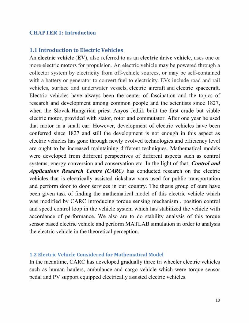
1.1 Introduction to Electric Vehicles

An electric vehicle (EV), also referred to as an electric drive vehicle, uses one or

more electric motors for propulsion. An electric vehicle may be powered through a

collector system by electricity from off-vehicle sources, or may be self-contained

with a battery or generator to convert fuel to electricity. EVs include road and rail

vehicles, surface and underwater vessels, electric aircraft and electric spacecraft.

Electric vehicles have always been the center of fascination and the topics of

research and development among common people and the scientists since 1827,

when the Slovak-Hungarian priest Anyos Jedlik built the first crude but viable

electric motor, provided with stator, rotor and commutator. After one year he used

that motor in a small car. However, development of electric vehicles have been

conferred since 1827 and still the development is not enough in this aspect as

electric vehicles has gone through newly evolved technologies and efficiency level

are ought to be increased maintaining different techniques. Mathematical models

were developed from different perspectives of different aspects such as control

systems, energy conversion and conservation etc. In the light of that, Control and

Applications Research Centre (CARC) has conducted research on the electric

vehicles that is electrically assisted rickshaw vans used for public transportation

and perform door to door services in our country. The thesis group of ours have

been given task of finding the mathematical model of this electric vehicle which

was modified by CARC introducing torque sensing mechanism , position control

and speed control loop in the vehicle system which has stabilized the vehicle with

accordance of performance. We also are to do stability analysis of this torque

sensor based electric vehicle and perform MATLAB simulation in order to analysis

the electric vehicle in the theoretical perception.

1.2 Electric Vehicle Considered for Mathematical Model

In the meantime, CARC has developed gradually three tri wheeler electric vehicles

such as human haulers, ambulance and cargo vehicle which were torque sensor

pedal and PV support equipped electrically assisted electric vehicles.

11

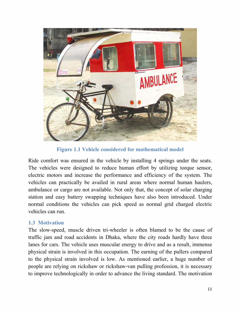
Figure 1.1 Vehicle considered for mathematical model

Ride comfort was ensured in the vehicle by installing 4 springs under the seats.

The vehicles were designed to reduce human effort by utilizing torque sensor,

electric motors and increase the performance and efficiency of the system. The

vehicles can practically be availed in rural areas where normal human haulers,

ambulance or cargo are not available. Not only that, the concept of solar charging

station and easy battery swapping techniques have also been introduced. Under

normal conditions the vehicles can pick speed as normal grid charged electric

vehicles can run.

1.3 Motivation

The slow-speed, muscle driven tri-wheeler is often blamed to be the cause of

traffic jam and road accidents in Dhaka, where the city roads hardly have three

lanes for cars. The vehicle uses muscular energy to drive and as a result, immense

physical strain is involved in this occupation. The earning of the pullers compared

to the physical strain involved is low. As mentioned earlier, a huge number of

people are relying on rickshaw or rickshaw-van pulling profession, it is necessary

to improve technologically in order to advance the living standard. The motivation

12

for working on this research and development program has been originated from

the observation that a substantial modernization in this sector will not only

improve the living standard of a huge number of people involved in rickshaw

pulling, but also improve the quality of life of upper and lower-middle income

group people. The electrically assisted rickshaw-van will relieve the pullers from

extreme physical exhaustion by assisting them electrically using torque sensor,

which will limit the over-use of battery bank. Solar panel will help in sharing the

load power and solar battery charging station will be used to charge the batteries

instead of using power from national grid. Thus, CARC has been making and

developing the technology for efficient use of renewable resources and making the

system completely independent of national grid. Our purpose of this research that

has been entrusted to us by CARC is to make the vehicles theoretically

approachable and define the vehicles in equations and doing the stability analysis

by thorough simulation process.

13

CHAPTER 2

Overview of the Whole System with Components

2.1 Introduction

The most common transportation vehicle in Dhaka city is rickshaw. Most of the

people like to ride on this for which day by day it becomes the first choice as a

public transportation. As Bangladesh is an under developed country, most of the

people of this country are underprivileged. Therefore, significant number of people

chooses their profession as a rickshaw puller. For the first time in Bangladesh

Beevatech Limited had developed a motorized rickshaw-van which has a multiple

input i.e. throttle and torque sensor pedal under the supervision of Control and

Applications Research Centre (CARC) of BRAC University. As the government

has disapproved commercialization of such motorized vehicle due to consumption

of electricity from the already overloaded grid, our motive is to find a solution to

conserve power for such green electric rickshaw-van with the use of PV panel,

torque sensor pedal and solar battery charging station. The vehicle that we

considered in our mathematical model has a brushless DC gear motor, four 12V

25Ah sealed lead acid batteries connected in series, a controller unit, a throttle,

main power key, emergency motor stopper, traditional front wheel brake and an

extra rear wheel break, charge controller, charge indicator and other components

[2]. The details of all the components are mentioned in the following sections.

Here is the skeleton view of the vehicle which we consider for our mathematical

model is shown in Fig 2.1.

14

Figure 2.1 Skeleton View

2.2 Components considered for mathematical model

2.2.1 The Batteries

In the vehicle that we are considering, four sealed lead-acid batteries are used,

which are connected in series. The dimension of each battery is 16.5 × 17.5 × 12.6

cm. Each of the battery is 12V, 25 Ah rechargeable which supplies 48 Volts to the

BLDC motor. The batteries are placed under both the seats as shown in Fig 2.1. If

we fully charge each of the battery it shows 12.7 volts across their terminals and

50.8 volts together as we connect the batteries in series [2].

15

Figure 2.2 Two batteries

2.2.2 The Motor

The vehicle that we are considering, uses a brushless DC gear motor which has a,

which has a power of 500 Watt and 500-550 rpm speed. This motor has a rated

current and voltage of 13.4A and 48V which is attached with the main frame. It is

mounted under the seat as shown in Fig 2.3. As this produces more torque per watt

that’s why it is very preferable for such kind of vehicles which linearly decreases

as velocity decreases.

16

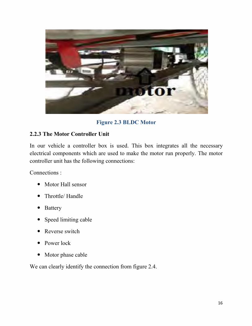
Figure 2.3 BLDC Motor

2.2.3 The Motor Controller Unit

In our vehicle a controller box is used. This box integrates all the necessary

electrical components which are used to make the motor run properly. The motor

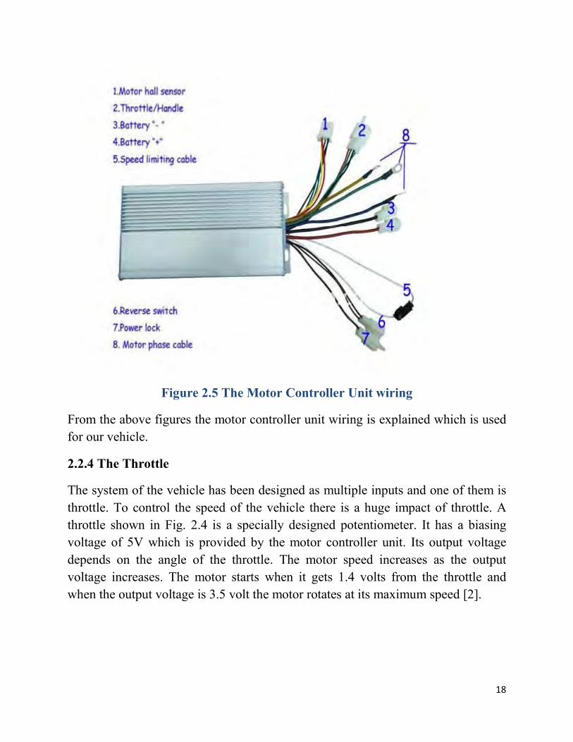
controller unit has the following connections:

Connections :

Motor Hall sensor

Throttle/ Handle

Battery

Speed limiting cable

Reverse switch

Power lock

Motor phase cable

We can clearly identify the connection from figure 2.4.

17

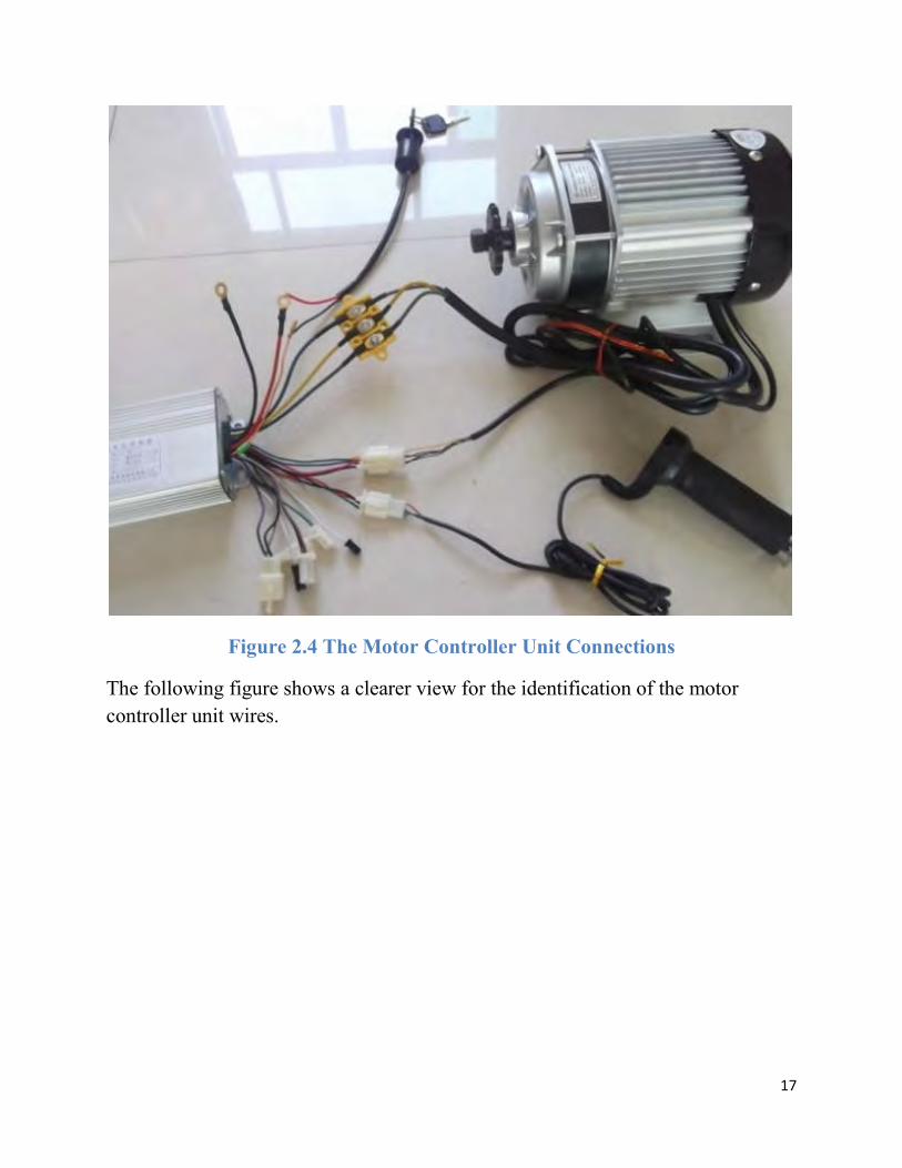
Figure 2.4 The Motor Controller Unit Connections

The following figure shows a clearer view for the identification of the motor

controller unit wires.

18

Figure 2.5 The Motor Controller Unit wiring

From the above figures the motor controller unit wiring is explained which is used

for our vehicle.

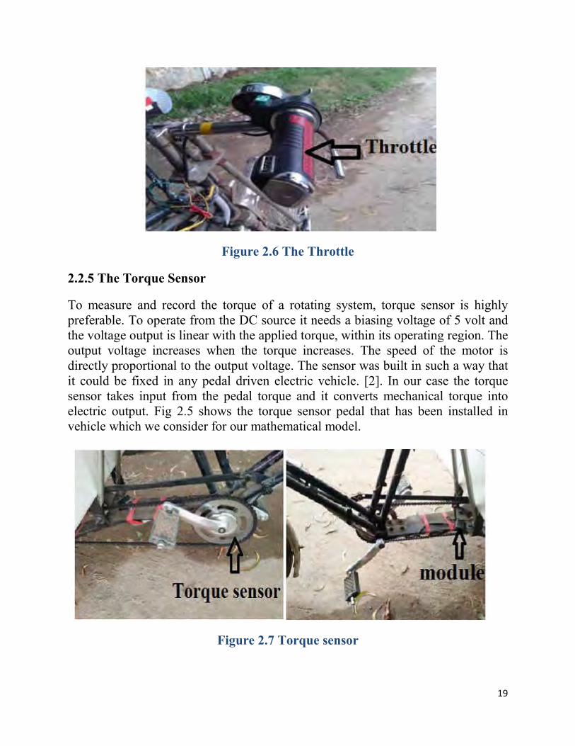
2.2.4 The Throttle

The system of the vehicle has been designed as multiple inputs and one of them is

throttle. To control the speed of the vehicle there is a huge impact of throttle. A

throttle shown in Fig. 2.4 is a specially designed potentiometer. It has a biasing

voltage of 5V which is provided by the motor controller unit. Its output voltage

depends on the angle of the throttle. The motor speed increases as the output

voltage increases. The motor starts when it gets 1.4 volts from the throttle and

when the output voltage is 3.5 volt the motor rotates at its maximum speed [2].

19

Figure 2.6 The Throttle

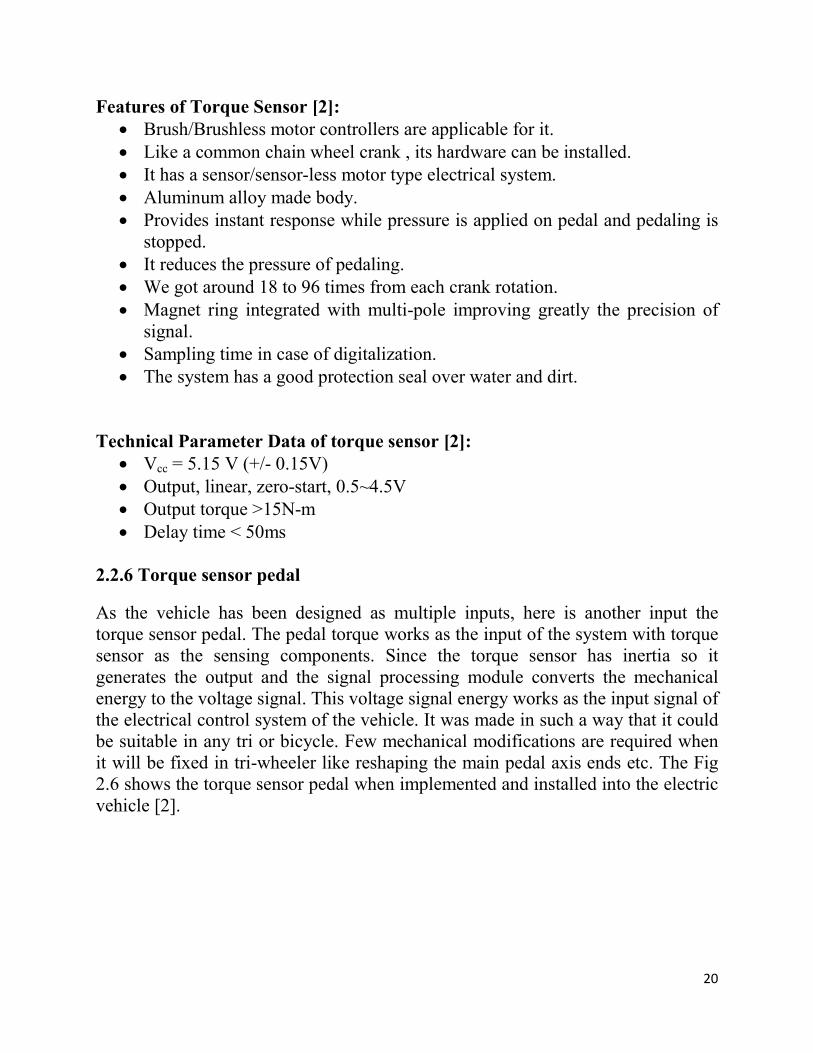
2.2.5 The Torque Sensor

To measure and record the torque of a rotating system, torque sensor is highly preferable. To operate from the DC source it needs a biasing voltage of 5 volt and the voltage output is linear with the applied torque, within its operating region. The output voltage increases when the torque increases. The speed of the motor is directly proportional to the output voltage. The sensor was built in such a way that it could be fixed in any pedal driven electric vehicle. [2]. In our case the torque sensor takes input from the pedal torque and it converts mechanical torque into electric output. Fig 2.5 shows the torque sensor pedal that has been installed in vehicle which we consider for our mathematical model.

Figure 2.7 Torque sensor

20

Features of Torque Sensor [2]: Brush/Brushless motor controllers are applicable for it. Like a common chain wheel crank , its hardware can be installed. It has a sensor/sensor-less motor type electrical system. Aluminum alloy made body. Provides instant response while pressure is applied on pedal and pedaling is

stopped. It reduces the pressure of pedaling. We got around 18 to 96 times from each crank rotation. Magnet ring integrated with multi-pole improving greatly the precision of

signal. Sampling time in case of digitalization. The system has a good protection seal over water and dirt.

Technical Parameter Data of torque sensor [2]:

Vcc = 5.15 V (+/- 0.15V) Output, linear, zero-start, 0.5~4.5V Output torque >15N-m Delay time < 50ms

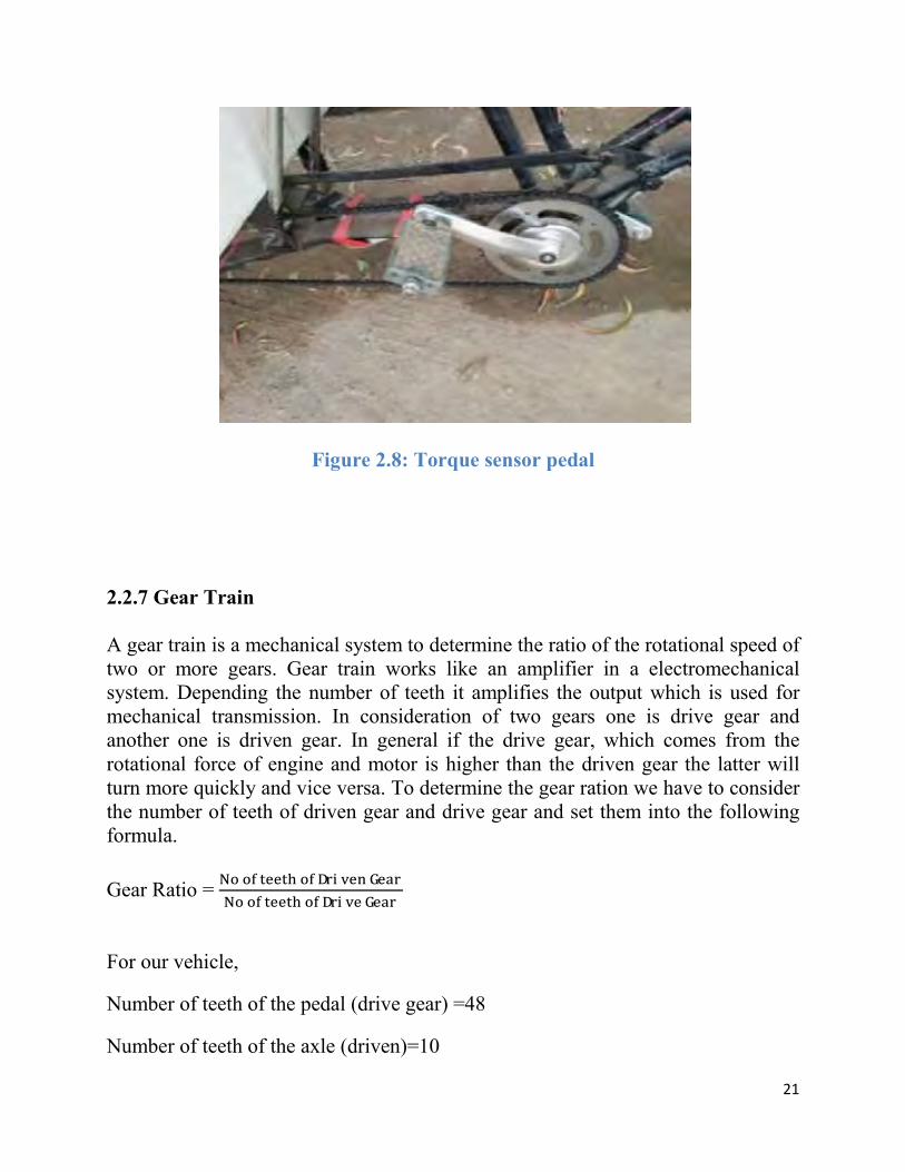
2.2.6 Torque sensor pedal

As the vehicle has been designed as multiple inputs, here is another input the torque sensor pedal. The pedal torque works as the input of the system with torque sensor as the sensing components. Since the torque sensor has inertia so it generates the output and the signal processing module converts the mechanical energy to the voltage signal. This voltage signal energy works as the input signal of the electrical control system of the vehicle. It was made in such a way that it could be suitable in any tri or bicycle. Few mechanical modifications are required when it will be fixed in tri-wheeler like reshaping the main pedal axis ends etc. The Fig 2.6 shows the torque sensor pedal when implemented and installed into the electric vehicle [2].

21

Figure 2.8: Torque sensor pedal

2.2.7 Gear Train A gear train is a mechanical system to determine the ratio of the rotational speed of two or more gears. Gear train works like an amplifier in a electromechanical system. Depending the number of teeth it amplifies the output which is used for mechanical transmission. In consideration of two gears one is drive gear and another one is driven gear. In general if the drive gear, which comes from the rotational force of engine and motor is higher than the driven gear the latter will turn more quickly and vice versa. To determine the gear ration we have to consider the number of teeth of driven gear and drive gear and set them into the following formula.

Gear Ratio = ��

��

For our vehicle,

Number of teeth of the pedal (drive gear) =48

Number of teeth of the axle (driven)=10

22

Figure 2.9 Gear Train

2.3 Conclusion

The electric vehicle that we are considering has got many other components

installed in it, which are necessary to run the vehicle. For the mathematical model,

those components are not required. We are only considering the electric and

mechanical components which are needed for the mathematical model.

23

CHAPTER 3: Developing Mathematical Model

3.1 Introduction

In order to develop a mathematical model, we need to build up a schematic of the

physical system first from which the mathematical interpretation will be done.

Mathematical model can be derived using two methods-

a) Transfer functions in the frequency domain

b) State equations in the time domain

In any case, the first step to derive a mathematical model is to apply fundamental

physical laws of science and engineering [1]. For instance, in case of modeling

electrical networks, Ohm’s laws and Kirchhoff’s laws are applied. For mechanical

system, we used Newton’s laws as fundamental guiding principle [1]. In our thesis,

we used the first of the two aforementioned methods for mathematical model. The

model shaped as transfer function relates the input of the system to its output

response. The reason for selecting the method is to represent the inputs, output and

the system distinctly and separately. According to Nise (2015), a system

represented by differential equation is difficult to model as a block diagram. Thus

here comes the idea of Laplace transformation, with which input, output and the

system can be represented individually. Not only will that, relationship between

them will become algebraic.

R(s) C(s)

Where R(s) is reference input and C(s) is output represented in frequency domain.

System

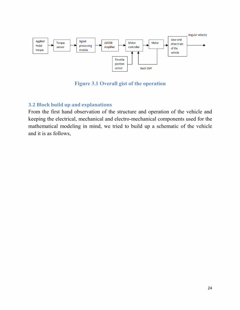
Figure 3.

3.2 Block build up and explanations

From the first hand observation of the structure and operation of the vehicle and

keeping the electrical, mechanical and electro

mathematical modeling in mind, we tried to build up a schematic of the vehicle

and it is as follows,

Figure 3.1 Overall gist of the operation

Block build up and explanations


ng the electrical, mechanical and electro-mechanical components used for the


24


mechanical components used for the


25

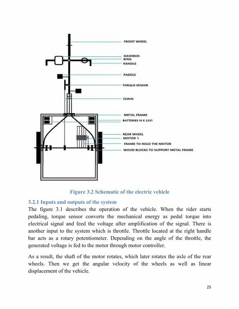
Figure 3.2 Schematic of the electric vehicle

3.2.1 Inputs and outputs of the system

The figure 3.1 describes the operation of the vehicle. When the rider starts

pedaling, torque sensor converts the mechanical energy as pedal torque into

electrical signal and feed the voltage after amplification of the signal. There is

another input to the system which is throttle. Throttle located at the right handle

bar acts as a rotary potentiometer. Depending on the angle of the throttle, the

generated voltage is fed to the motor through motor controller.

As a result, the shaft of the motor rotates, which later rotates the axle of the rear

wheels. Then we get the angular velocity of the wheels as well as linear

displacement of the vehicle.

Figure 3.3 F

3.3 Mathematical representation of the system

From figure 3.2 mathematical representation of the system has been determined

from the identification of the electrical and mechanical functionality of block

subsystems. Block by block analysis has been done as the following.

3.3.1 Torque sensor voltage from the

Torque sensor or torque transducer is means to convert the mechanical input

(torque) to electrical signal. This is done by sensor attached in the crank set and a

signal processing module is used to serve the purpose. Biasing voltage of to

sensor is 5 volts and it generates output voltage corresponding to the torque applied

to the particular crank set [2]. The voltage output is linear with the applied torque.

The parameter data of the torque sensor is given below:

VCC= 5.15 V (+/- 0.15

Output linear, zero start, 0.5~4.5 V

Output torque >15 Nm

unctional block diagram of the system

Mathematical representation of the system

igure 3.2 mathematical representation of the system has been determined


subsystems. Block by block analysis has been done as the following.

Torque sensor voltage from the Pedal torque TP:



signal processing module is used to serve the purpose. Biasing voltage of to



The parameter data of the torque sensor is given below:

0.15 V)

Output linear, zero start, 0.5~4.5 V

Output torque >15 Nm

26

igure 3.2 mathematical representation of the system has been determined




signal processing module is used to serve the purpose. Biasing voltage of torque



27

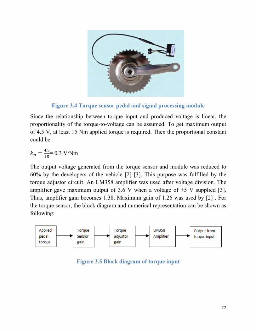
Figure 3.4 Torque sensor pedal and signal processing module

Since the relationship between torque input and produced voltage is linear, the

proportionality of the torque-to-voltage can be assumed. To get maximum output

of 4.5 V, at least 15 Nm applied torque is required. Then the proportional constant

could be

�� =�.�

��= 0.3 V/Nm

The output voltage generated from the torque sensor and module was reduced to

60% by the developers of the vehicle [2] [3]. This purpose was fulfilled by the

torque adjustor circuit. An LM358 amplifier was used after voltage division. The

amplifier gave maximum output of 3.6 V when a voltage of +5 V supplied [3].

Thus, amplifier gain becomes 1.38. Maximum gain of 1.26 was used by [2] . For

the torque sensor, the block diagram and numerical representation can be shown as

following:

Figure 3.5 Block diagram of torque input

Figure 3.6 Mathematical

Where,

�� = 0.3

�� = 0.6

�� = 1.26

3.3.2 Throttle Input:

As for throttle input, input torque T

used to control the speed of the motor. It is a rotary potentiometer with spring

attached internally. A specif

the motor controller unit and gives output as voltage corresponding to the angle

(��) of the throttle. Internal circuit diagram of the throttle is given in figure 3.5

Figure 3.7 Diagram for

Mathematical representation of the torque input

As for throttle input, input torque Tt has been introduced. Throttles are generally


A specific biasing voltage VCC is supplied to the throttle from


of the throttle. Internal circuit diagram of the throttle is given in figure 3.5

Diagram for a Throttle Position sensor

28

representation of the torque input

has been introduced. Throttles are generally


is supplied to the throttle from


of the throttle. Internal circuit diagram of the throttle is given in figure 3.5

29

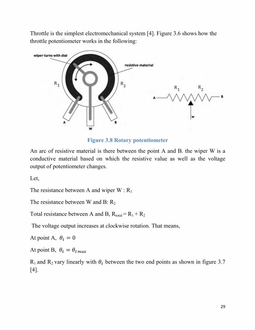
Throttle is the simplest electromechanical system [4]. Figure 3.6 shows how the

throttle potentiometer works in the following:

Figure 3.8 Rotary potentiometer

An arc of resistive material is there between the point A and B. the wiper W is a

conductive material based on which the resistive value as well as the voltage

output of potentiometer changes.

Let,

The resistance between A and wiper W : R1

The resistance between W and B: R2

Total resistance between A and B, Rtotal = R1 + R2

The voltage output increases at clockwise rotation. That means,

At point A, �� = 0

At point B, �� = ��

R1 and R2 vary linearly with �� between the two end points as shown in figure 3.7

[4].

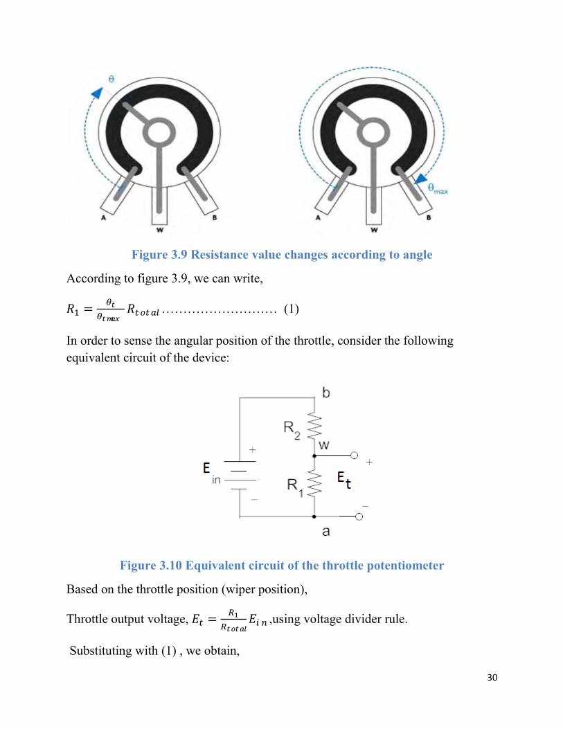
Figure 3.9 Resistance value changes

According to figure 3.9, we can write,

�� =��

�� ……………………… (1)

In order to sense the angular position of the throttle, consider the followi

equivalent circuit of the device:

Figure 3.10 Equivalent circuit of the throttle potentiometer

Based on the throttle position (wiper position),

Throttle output voltage, �� =

Substituting with (1) , we obtain,

Resistance value changes according to angle

, we can write,

……………………… (1)

In order to sense the angular position of the throttle, consider the followi

equivalent circuit of the device:

Equivalent circuit of the throttle potentiometer

Based on the throttle position (wiper position),

=��

�� ,using voltage divider rule.

ng with (1) , we obtain,

30

according to angle

……………………… (1)

In order to sense the angular position of the throttle, consider the following

Equivalent circuit of the throttle potentiometer

31

�� =

��

��

��

�� =��

��

��

��=

��

��…………………………………………………….....(2)

Considering the spring which tends to rotate back to its original position and in

terms of torque input to the throttle,

�� = ��, using Hooke’s Law.

Where, �� is a spring constant.

Substituting with equation (2), the equation yields as following,

�� =��

��

�� =��

��

��

��=

��

��= ��, which is a throttle constant.

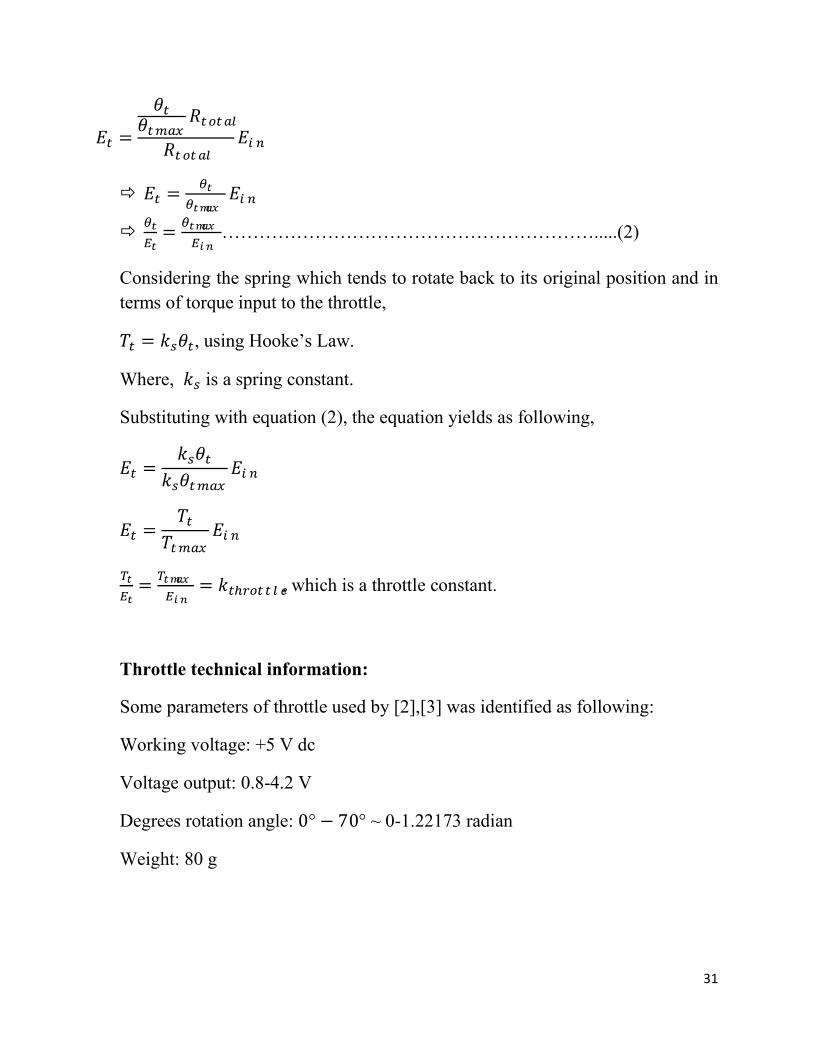
Throttle technical information:

Some parameters of throttle used by [2],[3] was identified as following:

Working voltage: +5 V dc

Voltage output: 0.8-4.2 V

Degrees rotation angle: 0° − 70° ~ 0-1.22173 radian

Weight: 80 g

Throttle Constant, ��

From Hooke’s law,

�� = ��

��

��=

�

�� ……………………………

Figure 3.11

For potentiometer gain, from (2) and (3) we find,

��

��=

��

��∗

��

��

��

��=

��

��∗

1

��=

��

��

To rotate at maximum (70 degree~1.22173

force on throttle,

�� =

Multiplying by radius (r=0.5 in ~ 0.0127 m) of the throttle, we get,

�� =

Maximum throttle output voltage,

Maximum angle deflection,

Spring constant, �� =��

��

��:

……………………………………………………..(3)

Figure 3.11 Block diagram for throttle

For potentiometer gain, from (2) and (3) we find,

aximum (70 degree~1.22173 rad), assumed maximum exerted

= .150�� ∗ 9.81� �� = 1.4715 �

Multiplying by radius (r=0.5 in ~ 0.0127 m) of the throttle, we get,

= 1.4715� ∗ 0.0125� = 0.018 ��

voltage, �� = 4.2 �

Maximum angle deflection, �� = 1.22173 rad

��

��=

�.��∗�.��

�∗�.�= 0.001 Nm/rad

32

maximum exerted

��

��= 244.346 , throttle gain which gives maxi

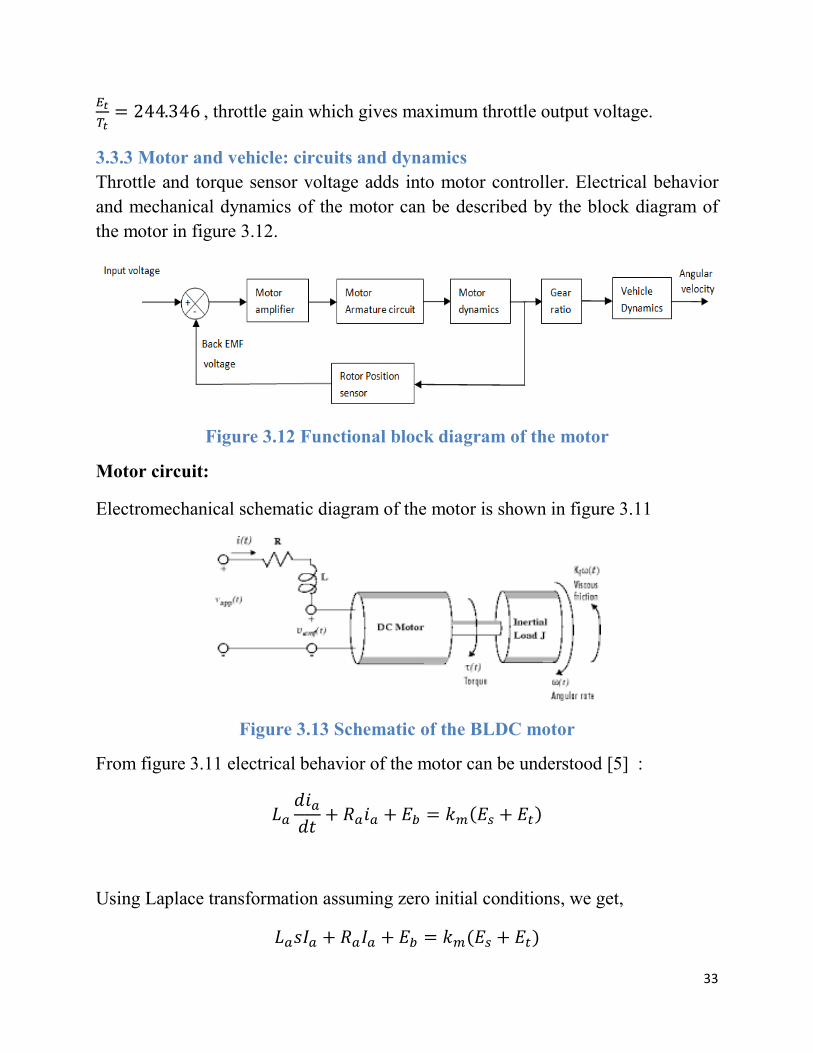
3.3.3 Motor and vehicle: circuits and dynamics

Throttle and torque sensor voltage adds into motor controller. Electrical behavior

and mechanical dynamics of the motor can be described by the

the motor in figure 3.12.

Figure 3.12 Functional block diagram of the motor

Motor circuit:

Electromechanical schematic

Figure 3.13

From figure 3.11 electrical behavior

��

�

��

Using Laplace transformation

��

, throttle gain which gives maximum throttle output voltage.

circuits and dynamics

torque sensor voltage adds into motor controller. Electrical behavior

and mechanical dynamics of the motor can be described by the block diagram

Functional block diagram of the motor

schematic diagram of the motor is shown in figure 3.11

Figure 3.13 Schematic of the BLDC motor

lectrical behavior of the motor can be understood [5]

��

��+ �� + �� = ��(�� + ��)

Using Laplace transformation assuming zero initial conditions, we get,

�� + �� + �� = ��(�� + ��)

33

mum throttle output voltage.

torque sensor voltage adds into motor controller. Electrical behavior

block diagram of

Functional block diagram of the motor

diagram of the motor is shown in figure 3.11

[5] :

, we get,

34

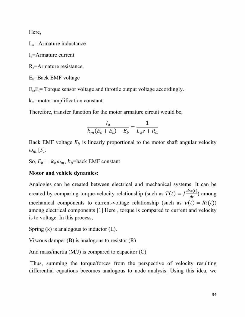
Here,

La= Armature inductance

Ia=Armature current

Ra=Armature resistance.

Eb=Back EMF voltage

Es,Et= Torque sensor voltage and throttle output voltage accordingly.

km=motor amplification constant

Therefore, transfer function for the motor armature circuit would be,

��

��(�� + ��)− ��=

1

�� + ��

Back EMF voltage �� is linearly proportional to the motor shaft angular velocity

�� [5].

So, �� = ��, ��=back EMF constant

Motor and vehicle dynamics:

Analogies can be created between electrical and mechanical systems. It can be

created by comparing torque-velocity relationship (such as �(�)= ��(�)

��) among

mechanical components to current-voltage relationship (such as �(�)= ��(�))

among electrical components [1].Here , torque is compared to current and velocity

is to voltage. In this process,

Spring (k) is analogous to inductor (L).

Viscous damper (B) is analogous to resistor (R)

And mass/inertia (M/J) is compared to capacitor (C)

Thus, summing the torque/forces from the perspective of velocity resulting

differential equations becomes analogous to node analysis. Using this idea, we

tried to create an analogous circuit for the dynamics of the vehicle

in figure 3.14

��(�)

Figure 3.14 T-i analogous

From the above figure we can find the motor dynamics equation

transformation assuming zero initial conditions

��(�) = ��(�)+ + ��

Where,

��=motor torque

��=motor inertia

��=viscous damping co-efficient of motor

��=Load torque of the motor

Load torque produces wheel torque (

Gear ratio in terms torque and

Hence, for vehicle dynamics, without considering the resistance torque [5], we get,

��(�)∗

tried to create an analogous circuit for the dynamics of the vehicle in consideration

��(�)

i analogous circuit for motor and vehicle dynamics

can find the motor dynamics equation in Laplace

transformation assuming zero initial conditions.

��(�)+ ��(�) ………………………………… (a)

efficient of motor

=Load torque of the motor

Load torque produces wheel torque (��) after gear transmission.

in terms torque and velocity, � =��

��=

� �

� �

�� =��

�

for vehicle dynamics, without considering the resistance torque [5], we get,

� = �� = ��(�)+ ��(�)

35

in consideration

for motor and vehicle dynamics

in Laplace

………………………………… (a)

for vehicle dynamics, without considering the resistance torque [5], we get,

36

=> ��(�)= �

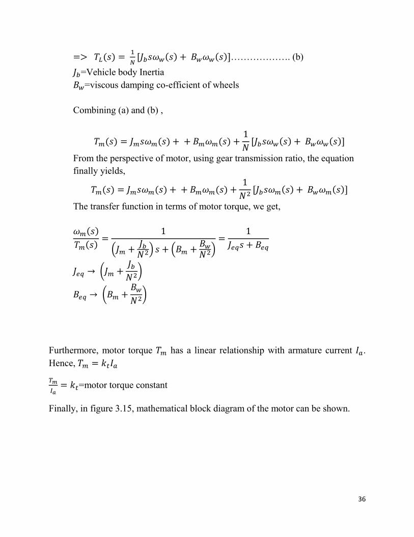
�[��(�)+ ��(�)]………………. (b)

��=Vehicle body Inertia

��=viscous damping co-efficient of wheels

Combining (a) and (b) ,

��(�) = ��(�)+ + ��(�)+1

�[��(�)+ ��(�)]

From the perspective of motor, using gear transmission ratio, the equation

finally yields,

��(�) = ��(�)+ + ��(�)+1

� �[��(�)+ ��(�)]

The transfer function in terms of motor torque, we get,

��(�)

��(�)=

1

�� +��

� �� + �� +��

� ��=

1

�� + ��

�� → �� +��

� ��

�� → �� +��

� ��

Furthermore, motor torque �� has a linear relationship with armature current �� .

Hence, �� = ��

��

��= ��=motor torque constant

Finally, in figure 3.15, mathematical block diagram of the motor can be shown.

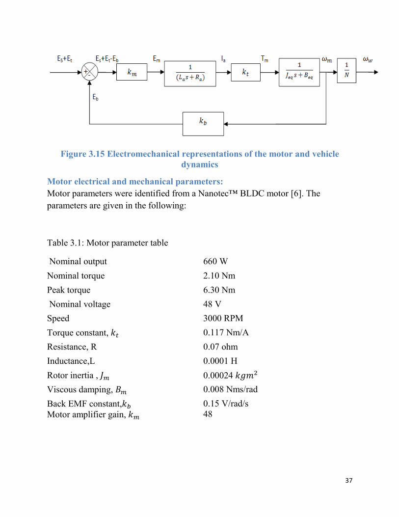
Figure 3.15 Electromechanical r

Motor electrical and mechanical parameters:

Motor parameters were identified from a Nanotec

parameters are given in the following:

Table 3.1: Motor parameter table

Nominal output

Nominal torque

Peak torque

Nominal voltage

Speed

Torque constant, ��

Resistance, R

Inductance,L

Rotor inertia , ��

Viscous damping, ��

Back EMF constant,�� Motor amplifier gain, ��

Electromechanical representations of the motor and vehicle dynamics

chanical parameters:

Motor parameters were identified from a Nanotec™ BLDC motor [6].

parameters are given in the following:

1: Motor parameter table

660 W

2.10 Nm

6.30 Nm

48 V

3000 RPM

0.117 Nm/A

0.07 ohm

0.0001 H

0.00024 ��

0.008 Nms/rad

0.15 V/rad/s 48

37

epresentations of the motor and vehicle

motor [6]. The

38

As for the inertia acting on the wheel, the wheel has a cylindrical radius [7] and

thus, estimating for m=250 kg load and radius r=13 inch~0.3302 m,

�� =1

2� �� = 0.5 ∗ 250 ∗ 0.3302� = 13.63 ��

�� at rated speed=3000 RPM~314.16 rad/s

At 70% efficiency of motor, �� = 314.16 ∗�

�.��= 448.8 rad/s

As well as, �� =��∗�.��∗�.��

��.�= 1.8 Nm/rad/s

�� = �� +��

� �= 0.0024 +

13.63

0.7�= 27.82 ��

�� = �� +��

� �= 0.008 +

�.�

�.��= 3.68 Nm/rad/s

3.3.4 Mathematical model of the overall system

Combining the block diagrams from figure 3.6, 3.11 and 3.15, we obtain the final

mathematical block diagram of the system.

From figure 3.6, substituting all the constants ��,�� & ��for �� ,

�� = �� ∗ �� ∗ ��

From figure 3.11,

��= ��

��

and from figure 3.15,

�� = �� + �� − ��

Finally the block diagram for the full system in figure 3.16

Figure 3.16 Mathematical block diagram of the full system

Derivation of final equation

Using superposition principle,

1) When �� active, �� =

a)

Figure 3.17 Block diagram for only pedal input

b) Using block diagram manipulation

following:

Mathematical block diagram of the full system

Derivation of final equation

Using superposition principle,

0

7 Block diagram for only pedal input

Using block diagram manipulation technique, figure 3.15 can be changed as

39

Mathematical block diagram of the full system

technique, figure 3.15 can be changed as

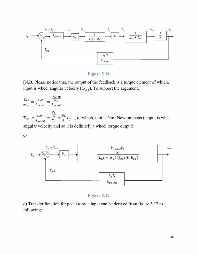
[N.B. Please notice that, the output of the feedback is a torque element of which,

input is wheel angular velocity (

��

��=

��

��=

��

��

�� =��

��=

� ��

��=

��

��

angular velocity and so it is definitely a wh

c)

d) Transfer function for pedal torque input can be derived from figure 3.17 as

following:

Figure 3.18


input is wheel angular velocity (��). To support the argument,

; of which, unit is Nm (Newton meter), input is wheel

angular velocity and so it is definitely a wheel torque output]

Figure 3.19


40


, input is wheel


��

��=

��

1 +��

=��

e) Let, � ′ =��

� , then,

��

��=

��

2) �� active, �� = 0

i)

��/�

�� + �� + �� + ��

��/�

�� + �� + �� + ��

��

��

�� + �� + �� + �� + �

, then,

� ′

�� + �� + �� + �� + ��

Figure 3.20

Figure 3.21

41

��

��

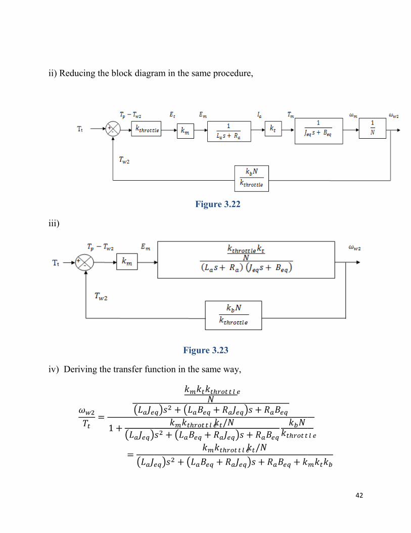
ii) Reducing the block diagram in the same procedure,

iii)

iv) Deriving the transfer function in the same way,

��

��=

��

1 +��

=��

ii) Reducing the block diagram in the same procedure,

Figure 3.22

Figure 3.23

iv) Deriving the transfer function in the same way,

��

�� + �� + �� + ��

��/�

�� + �� + �� + ��

��

��/�

� �� + �� + �� + �� + �

42

��

��

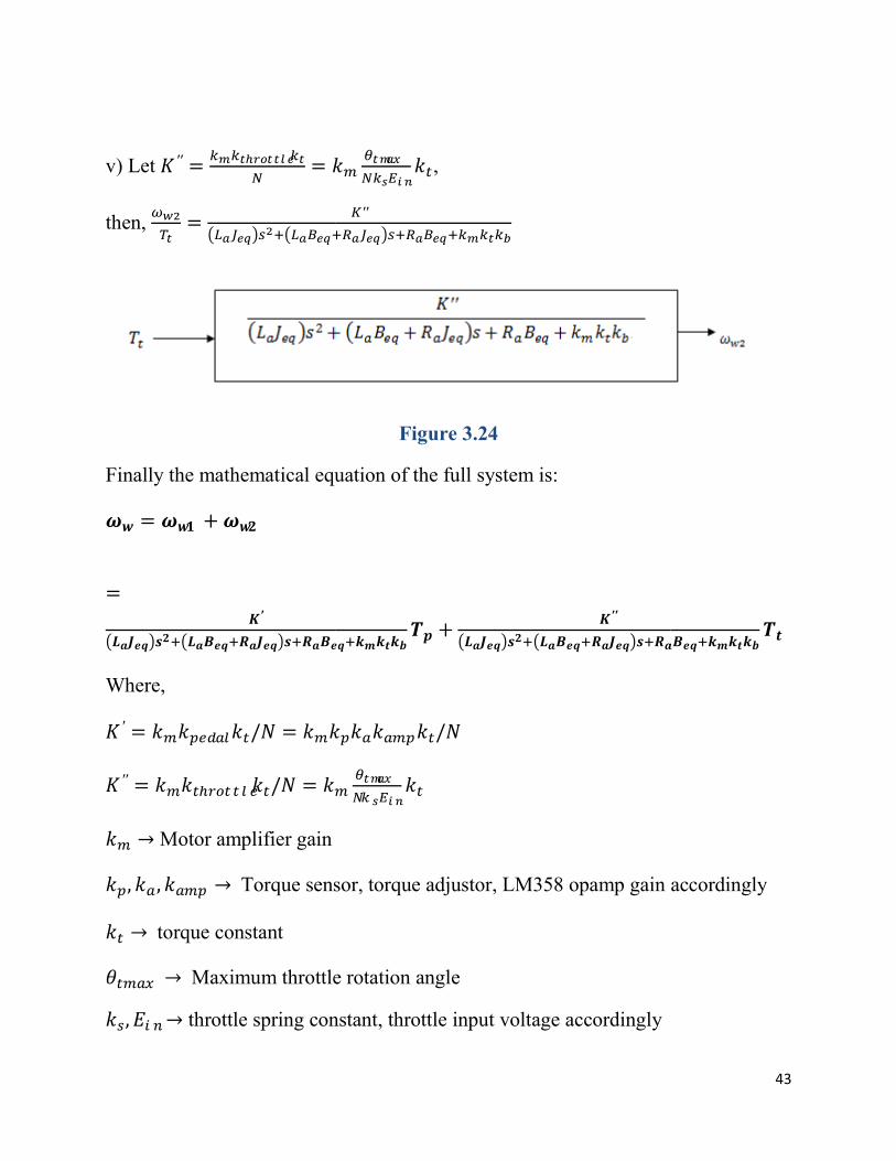
v) Let � ′′ =��

�= �

then, ��

��=

��

Finally the mathematical equation of the full system is:

� � = � �� + � ��

=� ′

��

Where,

� ′ = ��/� = ��

� ′′ = ��/� = ��

�� → Motor amplifier gain

��,��,�� → Torque sensor, torque adjustor, LM358 opamp gain accordingly

�� → torque constant

�� → Maximum throttle rotation angle

��,�� → throttle spring constant, throttle input voltage accordingly

��

� ��,

� ′′

��

Figure 3.24

Finally the mathematical equation of the full system is:

�� +

� ′′

��

��/�

��

��

Torque sensor, torque adjustor, LM358 opamp gain accordingly

Maximum throttle rotation angle

throttle spring constant, throttle input voltage accordingly

43

� ��

Torque sensor, torque adjustor, LM358 opamp gain accordingly

44

� → Gear ratio

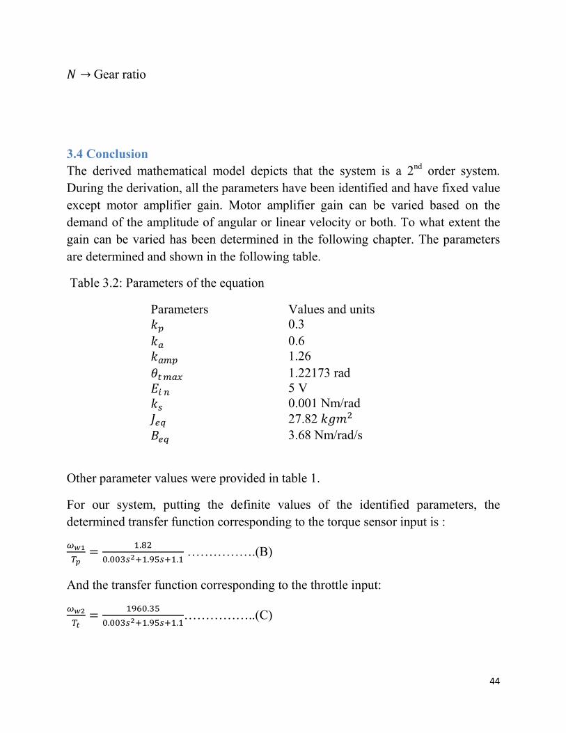
3.4 Conclusion

The derived mathematical model depicts that the system is a 2nd order system.

During the derivation, all the parameters have been identified and have fixed value

except motor amplifier gain. Motor amplifier gain can be varied based on the

demand of the amplitude of angular or linear velocity or both. To what extent the

gain can be varied has been determined in the following chapter. The parameters

are determined and shown in the following table.

Table 3.2: Parameters of the equation

Parameters Values and units �� 0.3

�� 0.6 �� 1.26

�� 1.22173 rad �� 5 V �� 0.001 Nm/rad �� 27.82 ��

�� 3.68 Nm/rad/s

Other parameter values were provided in table 1.

For our system, putting the definite values of the identified parameters, the

determined transfer function corresponding to the torque sensor input is :

��

��=

�.��

�.��.��.� …………….(B)

And the transfer function corresponding to the throttle input:

��

��=

��.��

�.��.��.�……………..(C)

Chapter 4

System Analysis, MATLAB Simulation and Results

4.1 Introduction

In this chapter, we will try to find the range of motor amplifier gain using several

methods. Taking the value between the ranges, we can

value for obtaining the desired output.

simulation and comparison with real time situation will also be done here. For

stability analysis, we used Routh

the relative stability analysis between two input

used. The methods used for the system analysis will be discussed broadly in the

following sections.

4.2 Range of gain, �� determination

Root Locus technique is a graphical presentation of the closed loop poles as a

system parameter is varied [1]

way the parameter gain can be varied and their co

and close loop characteristic equation

poles vary when the system parameter or gain is changed [8].

4.2.1 Root locus plot for Pedal torque,

Recalling figure 3.19 we can see,

System Analysis, MATLAB Simulation and Results


Taking the value between the ranges, we can use any particular

value for obtaining the desired output. Moreover, system build up in MATLAB ,


we used Routh-Hurwitz stability criterion and Root loc

the relative stability analysis between two input responses, bode plot has been


determination using Root Locus Technique


system parameter is varied [1]. Analyzing the root locus we understand in which

way the parameter gain can be varied and their corresponding transient response

close loop characteristic equation. Root locus plot shows how the closed loop

poles vary when the system parameter or gain is changed [8].

Root locus plot for Pedal torque, ��

we can see,

45


any particular gain

Moreover, system build up in MATLAB ,


Hurwitz stability criterion and Root locus. For

, bode plot has been



. Analyzing the root locus we understand in which

rresponding transient response

Root locus plot shows how the closed loop

For root locus analysis, we assumed that

gain of the system. Henceforth, the close loop transfer function,

��

��=

�.��

�.��.��.��.��

Here, close loop gain is ��

G(s)=

��

�

��

� =��

��= 0.463

To find the range of gain, the root locus plot was do

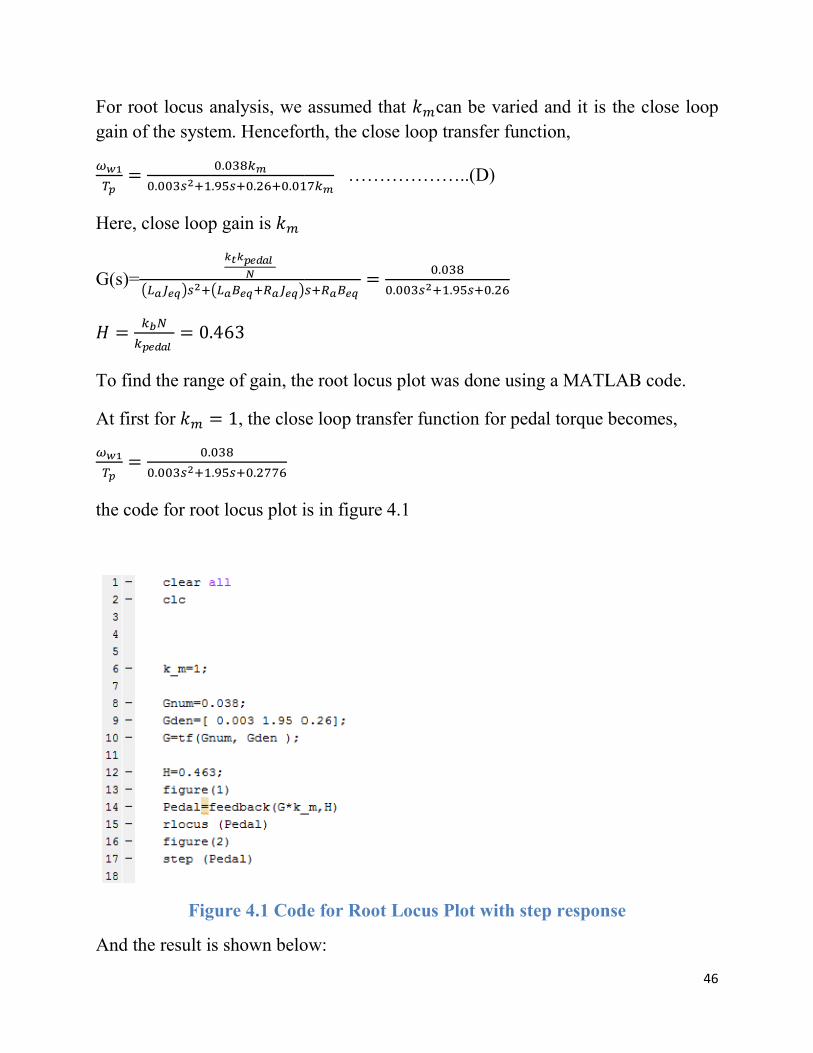
At first for �� = 1, the close loop transfer function for pedal torque becomes,

��

��=

�.��

�.��.��.��

the code for root locus plot is in figure 4.1

Figure 4.1 Code for Root Locus Plot with step

And the result is shown below:

For root locus analysis, we assumed that ��can be varied and it is the close loop

gain of the system. Henceforth, the close loop transfer function,

�� ………………..(D)

�� =

�.��

�.��.��.��

find the range of gain, the root locus plot was done using a MATLAB code.

the close loop transfer function for pedal torque becomes,

the code for root locus plot is in figure 4.1

Figure 4.1 Code for Root Locus Plot with step response

And the result is shown below:

46

can be varied and it is the close loop

ne using a MATLAB code.

the close loop transfer function for pedal torque becomes,

response

47

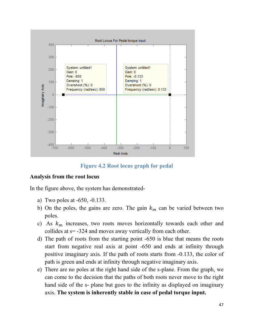
Figure 4.2 Root locus graph for pedal

Analysis from the root locus

In the figure above, the system has demonstrated-

a) Two poles at -650, -0.133.

b) On the poles, the gains are zero. The gain �� can be varied between two

poles.

c) As �� increases, two roots moves horizontally towards each other and

collides at s= -324 and moves away vertically from each other.

d) The path of roots from the starting point -650 is blue that means the roots

start from negative real axis at point -650 and ends at infinity through

positive imaginary axis. If the path of roots starts from -0.133, the color of

path is green and ends at infinity through negative imaginary axis.

e) There are no poles at the right hand side of the s-plane. From the graph, we

can come to the decision that the paths of both roots never move to the right

hand side of the s- plane but goes to the infinity as displayed on imaginary

axis. The system is inherently stable in case of pedal torque input.

f) On the real axis, gain can be varied from 4.5

4.2.2 Root locus plot for throttle input,

Recalling the figure 3.23

The corresponding transfer function is:

��

��=

��.��

�.��.��.��.��

In order to put the values and functions in code,

Here,

G(s)= ��

��

H = ��

�� = 0.00042

For �� = 1,

The code is:

gain can be varied from 4.5-8300

4.2.2 Root locus plot for throttle input, ��

The corresponding transfer function is:

�� …………………..(E)

he values and functions in code,

�/�

�� =

��.��

�.��.��.��

48

49

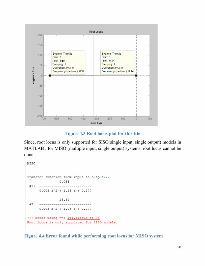
The result of the simulation of this code is as same as Pedal torque one . The path

of the two roots’ (-650 & -0.14) colliding point has not changed(s=-324) and at the

colliding point the gain, �� is 11.1. The system is inherently stable too for the

throttle input.

50

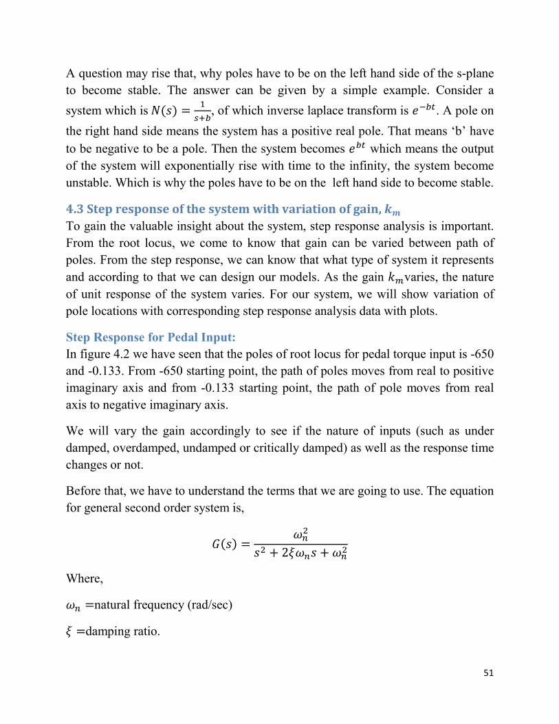
Figure 4.3 Root locus plot for throttle

Since, root locus is only supported for SISO(single input, single output) models in

MATLAB , for MISO (multiple input, single output) systems, root locus cannot be

done .

Figure 4.4 Error found while performing root locus for MISO system

51

A question may rise that, why poles have to be on the left hand side of the s-plane

to become stable. The answer can be given by a simple example. Consider a

system which is � (�) =�

��, of which inverse laplace transform is �� . A pole on

the right hand side means the system has a positive real pole. That means ‘b’ have

to be negative to be a pole. Then the system becomes �� which means the output

of the system will exponentially rise with time to the infinity, the system become

unstable. Which is why the poles have to be on the left hand side to become stable.

4.3 Step response of the system with variation of gain, ��

To gain the valuable insight about the system, step response analysis is important.

From the root locus, we come to know that gain can be varied between path of

poles. From the step response, we can know that what type of system it represents

and according to that we can design our models. As the gain ��varies, the nature

of unit response of the system varies. For our system, we will show variation of

pole locations with corresponding step response analysis data with plots.

Step Response for Pedal Input:

In figure 4.2 we have seen that the poles of root locus for pedal torque input is -650

and -0.133. From -650 starting point, the path of poles moves from real to positive

imaginary axis and from -0.133 starting point, the path of pole moves from real

axis to negative imaginary axis.

We will vary the gain accordingly to see if the nature of inputs (such as under

damped, overdamped, undamped or critically damped) as well as the response time

changes or not.

Before that, we have to understand the terms that we are going to use. The equation

for general second order system is,

�(�) =��

�

�� + 2�� + ��

Where,

�� =natural frequency (rad/sec)

� =damping ratio.

52

Natural frequency , �� is the frequency of oscillations without damping[1]. These

two quantities are the determinants of characteristics of a second order transient

response.

If, � > 1, the system is overdamped.

� = 1, the system is critically damped.

� < 1 , the system is underdamped.

Other parameters are as follows:

Rise time, ��: The time required to rise from low value to peak high value of the

transient response.

Peak time, ��: Time required to reach the peak value of the response.

% Overshoot: the amount of which the waveform overshoots the steady state or

final value at the peak time is expressed as the percentage of the steady state value

[1].

Settling time, ��: the time required for the transient’s damped oscillations to reach

and stay within ±2% of the steady state value (Nise,2015).

Example:

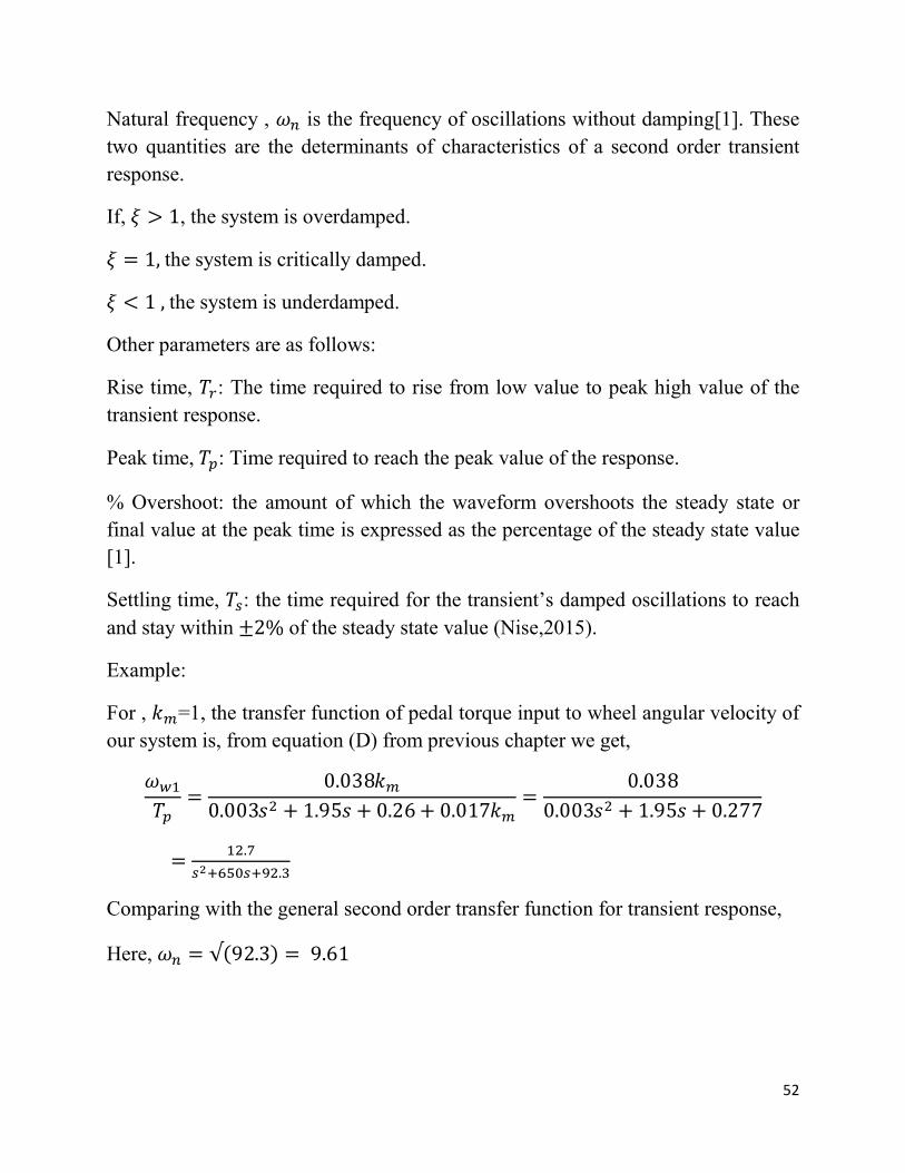
For , ��=1, the transfer function of pedal torque input to wheel angular velocity of

our system is, from equation (D) from previous chapter we get,

��

��=

0.038��

0.003�� + 1.95� + 0.26 + 0.017��=

0.038

0.003�� + 1.95� + 0.277

=��.�

��.�

Comparing with the general second order transfer function for transient response,

Here, �� = √(92.3)= 9.61

� =��

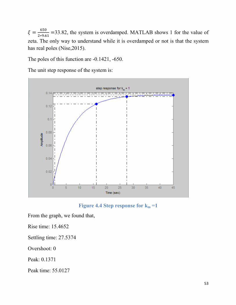
�∗�.��=33.82, the system is overdamped. MATLAB shows 1

zeta. The only way to understand while it is overdamped or not is that the system

has real poles (Nise,2015).

The poles of this function are

The unit step response of the system is:

Figure

From the graph, we found that,

Rise time: 15.4652

Settling time: 27.5374

Overshoot: 0

Peak: 0.1371

Peak time: 55.0127

33.82, the system is overdamped. MATLAB shows 1 for the value of


The poles of this function are -0.1421, -650.

The unit step response of the system is:

Figure 4.4 Step response for km =1

the graph, we found that,

53

for the value of


54

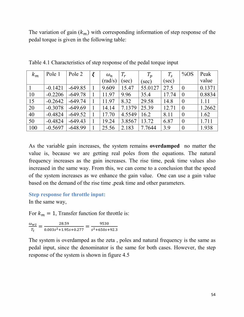
The variation of gain (��) with corresponding information of step response of the

pedal torque is given in the following table:

Table 4.1 Characteristics of step response of the pedal torque input

�� Pole 1 Pole 2 � �� (rad/s)

�� (sec)

��

(sec)

�� (sec)

%OS Peak value

1 -0.1421 -649.85 1 9.609 15.47 55.0127 27.5 0 0.1371 10 -0.2206 -649.78 1 11.97 9.96 35.4 17.74 0 0.8834 15 -0.2642 -649.74 1 11.97 8.32 29.58 14.8 0 1.11 20 -0.3078 -649.69 1 14.14 7.1379 25.39 12.71 0 1.2662 40 -0.4824 -649.52 1 17.70 4.5549 16.2 8.11 0 1.62 50 -0.4824 -649.43 1 19.24 3.8567 13.72 6.87 0 1.711 100 -0.5697 -648.99 1 25.56 2.183 7.7644 3.9 0 1.938

As the variable gain increases, the system remains overdamped no matter the

value is, because we are getting real poles from the equations. The natural

frequency increases as the gain increases. The rise time, peak time values also

increased in the same way. From this, we can come to a conclusion that the speed

of the system increases as we enhance the gain value. One can use a gain value

based on the demand of the rise time ,peak time and other parameters.

Step response for throttle input:

In the same way,

For �� = 1, Transfer function for throttle is:

��

��=

��.��

�.��.��.��=

��

��.�

The system is overdamped as the zeta , poles and natural frequency is the same as

pedal input, since the denominator is the same for both cases. However, the step

response of the system is shown in figure 4.5

55

Figure 4.5 Step response for throttle input

The information corresponding to the graph :

Rise time: 15.4652

Settling time: 27.5374

Overshoot: 0

Peak: 103.1714

Peak time: 55.0127

The peak is different but the other parameters are exactly the same as the step

response for pedal torque input. Henceforth, zeta, natural frequency and other time

parameters does not change while the amplitude of the response increases which

can be shown as below:

56

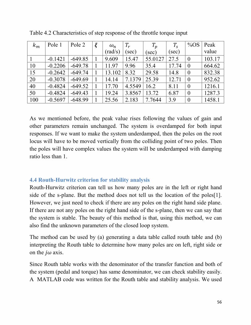
Table 4.2 Characteristics of step response of the throttle torque input

�� Pole 1 Pole 2 � �� (rad/s)

�� (sec)

�� (sec)

�� (sec)

%OS Peak value

1 -0.1421 -649.85 1 9.609 15.47 55.0127 27.5 0 103.17 10 -0.2206 -649.78 1 11.97 9.96 35.4 17.74 0 664.62 15 -0.2642 -649.74 1 13.102 8.32 29.58 14.8 0 832.38 20 -0.3078 -649.69 1 14.14 7.1379 25.39 12.71 0 952.62 40 -0.4824 -649.52 1 17.70 4.5549 16.2 8.11 0 1216.1 50 -0.4824 -649.43 1 19.24 3.8567 13.72 6.87 0 1287.3 100 -0.5697 -648.99 1 25.56 2.183 7.7644 3.9 0 1458.1

As we mentioned before, the peak value rises following the values of gain and

other parameters remain unchanged. The system is overdamped for both input

responses. If we want to make the system underdamped, then the poles on the root

locus will have to be moved vertically from the colliding point of two poles. Then

the poles will have complex values the system will be underdamped with damping

ratio less than 1.

4.4 Routh-Hurwitz criterion for stability analysis

Routh-Hurwitz criterion can tell us how many poles are in the left or right hand

side of the s-plane. But the method does not tell us the location of the poles[1].

However, we just need to check if there are any poles on the right hand side plane.

If there are not any poles on the right hand side of the s-plane, then we can say that

the system is stable. The beauty of this method is that, using this method, we can

also find the unknown parameters of the closed loop system.

The method can be used by (a) generating a data table called routh table and (b)

interpreting the Routh table to determine how many poles are on left, right side or

on the �� axis.

Since Routh table works with the denominator of the transfer function and both of

the system (pedal and torque) has same denominator, we can check stability easily.

A MATLAB code was written for the Routh table and stability analysis. We used

57

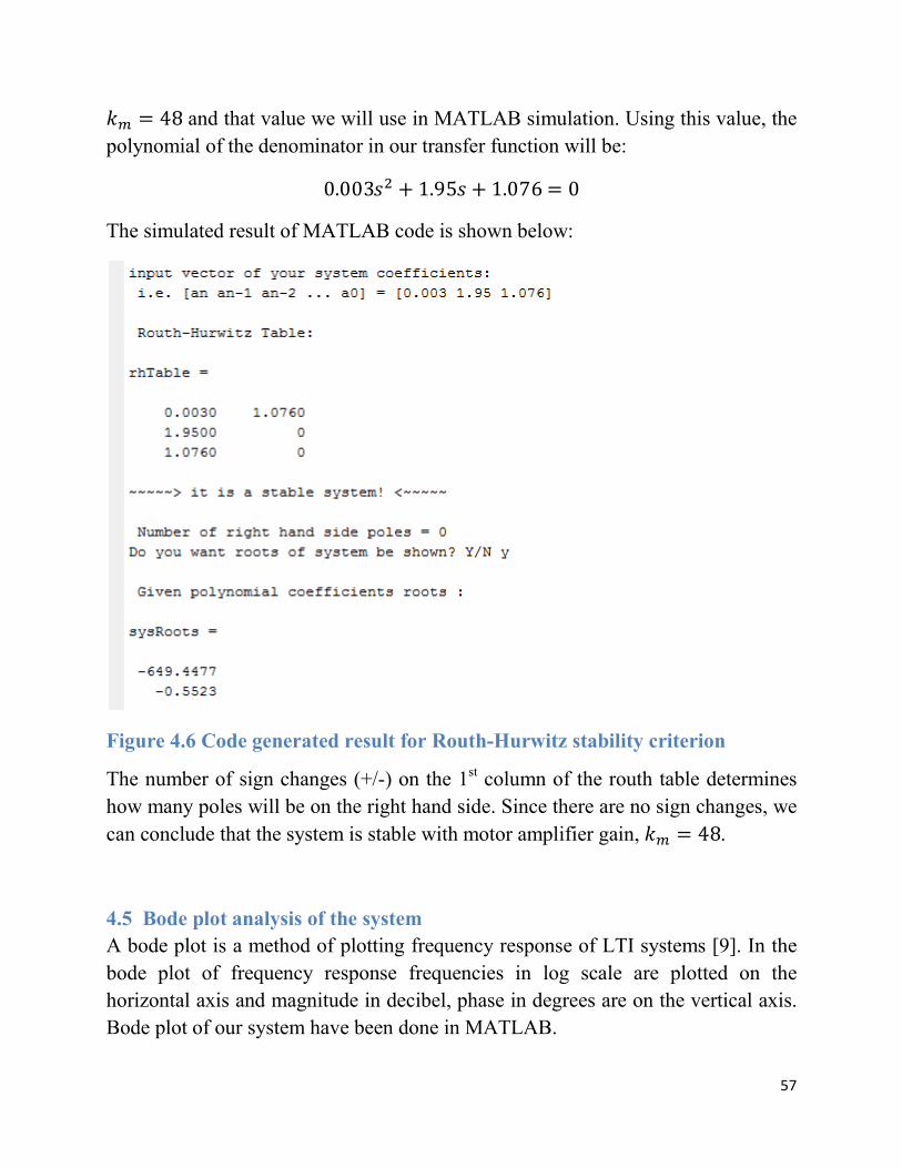
�� = 48 and that value we will use in MATLAB simulation. Using this value, the

polynomial of the denominator in our transfer function will be:

0.003�� + 1.95� + 1.076 = 0

The simulated result of MATLAB code is shown below:

Figure 4.6 Code generated result for Routh-Hurwitz stability criterion

The number of sign changes (+/-) on the 1st column of the routh table determines

how many poles will be on the right hand side. Since there are no sign changes, we

can conclude that the system is stable with motor amplifier gain, �� = 48.

4.5 Bode plot analysis of the system

A bode plot is a method of plotting frequency response of LTI systems [9]. In the

bode plot of frequency response frequencies in log scale are plotted on the

horizontal axis and magnitude in decibel, phase in degrees are on the vertical axis.

Bode plot of our system have been done in MATLAB.

58

Bode plot for pedal input

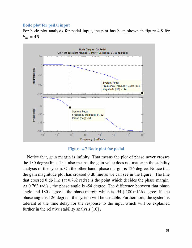
For bode plot analysis for pedal input, the plot has been shown in figure 4.8 for

�� = 48.

Figure 4.7 Bode plot for pedal

Notice that, gain margin is infinity. That means the plot of phase never crosses

the 180 degree line. That also means, the gain value does not matter in the stability

analysis of the system. On the other hand, phase margin is 126 degree. Notice that

the gain magnitude plot has crossed 0 db line as we can see in the figure. The line

that crossed 0 db line (at 0.762 rad/s) is the point which decides the phase margin.

At 0.762 rad/s , the phase angle is -54 degree. The difference between that phase

angle and 180 degree is the phase margin which is -54-(-180)=126 degree. If the

phase angle is 126 degree , the system will be unstable. Furthermore, the system is

tolerant of the time delay for the response to the input which will be explained

further in the relative stability analysis [10] .

59

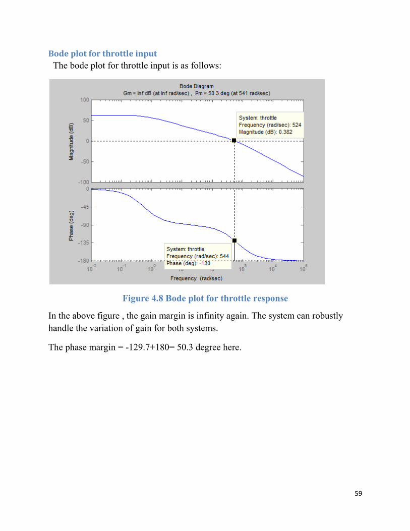
Bode plot for throttle input

The bode plot for throttle input is as follows:

Figure 4.8 Bode plot for throttle response

In the above figure , the gain margin is infinity again. The system can robustly

handle the variation of gain for both systems.

The phase margin = -129.7+180= 50.3 degree here.

60

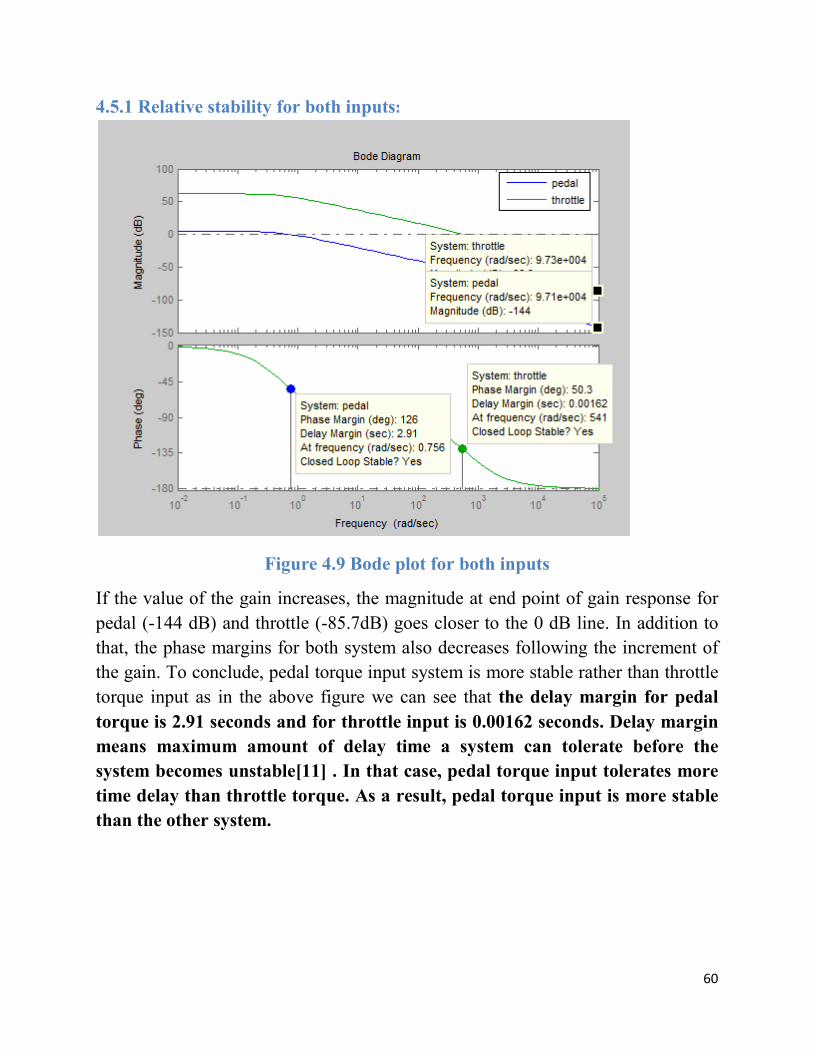
4.5.1 Relative stability for both inputs:

Figure 4.9 Bode plot for both inputs

If the value of the gain increases, the magnitude at end point of gain response for

pedal (-144 dB) and throttle (-85.7dB) goes closer to the 0 dB line. In addition to

that, the phase margins for both system also decreases following the increment of

the gain. To conclude, pedal torque input system is more stable rather than throttle

torque input as in the above figure we can see that the delay margin for pedal

torque is 2.91 seconds and for throttle input is 0.00162 seconds. Delay margin

means maximum amount of delay time a system can tolerate before the

system becomes unstable[11] . In that case, pedal torque input tolerates more

time delay than throttle torque. As a result, pedal torque input is more stable

than the other system.

61

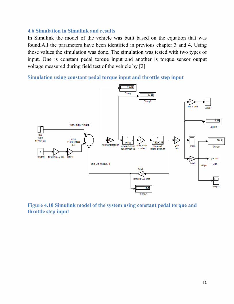
4.6 Simulation in Simulink and results

In Simulink the model of the vehicle was built based on the equation that was

found.All the parameters have been identified in previous chapter 3 and 4. Using

those values the simulation was done. The simulation was tested with two types of

input. One is constant pedal torque input and another is torque sensor output

voltage measured during field test of the vehicle by [2].

Simulation using constant pedal torque input and throttle step input

Figure 4.10 Simulink model of the system using constant pedal torque and throttle step input

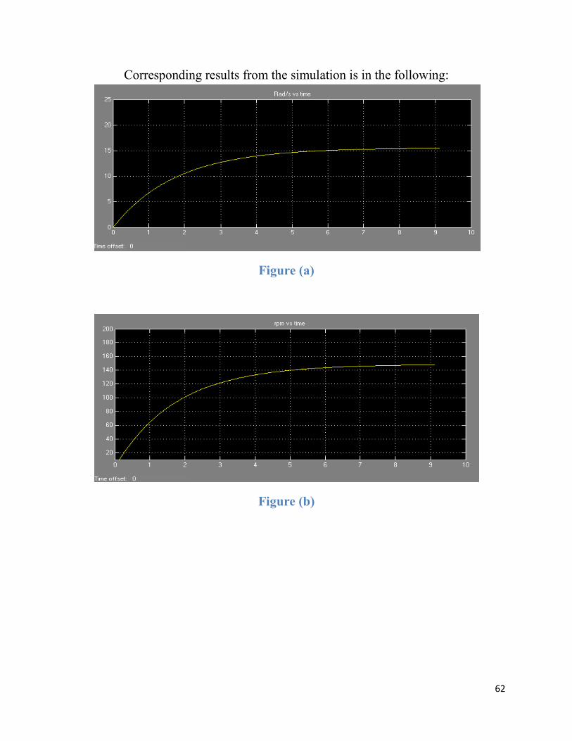
Corresponding results from the simulation is in the foll

Corresponding results from the simulation is in the following:

Figure (a)

Figure (b)

62

owing:

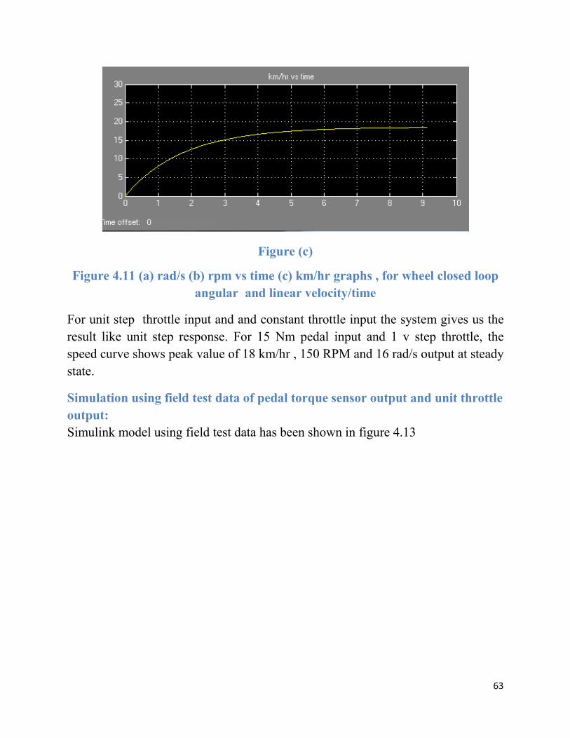
Figure 4.11 (a) rad/s (b) rpm vs time (c) km/hr graphs , for wheel closed loop

angular and linear velocity/time

For unit step throttle input and and constant throttle input the system gives us the

result like unit step response. For 15 Nm pedal input and 1 v step throttle, the

speed curve shows peak value of 18 km/hr , 150 RPM and 16 rad/s output at steady

state.

Simulation using field test data of pedal torque sensor output and unit throttle

output:

Simulink model using field test data has been shown in figure 4.13

Figure (c)

rad/s (b) rpm vs time (c) km/hr graphs , for wheel closed loop

angular and linear velocity/time


response. For 15 Nm pedal input and 1 v step throttle, the

curve shows peak value of 18 km/hr , 150 RPM and 16 rad/s output at steady


model using field test data has been shown in figure 4.13

63

rad/s (b) rpm vs time (c) km/hr graphs , for wheel closed loop


response. For 15 Nm pedal input and 1 v step throttle, the

curve shows peak value of 18 km/hr , 150 RPM and 16 rad/s output at steady


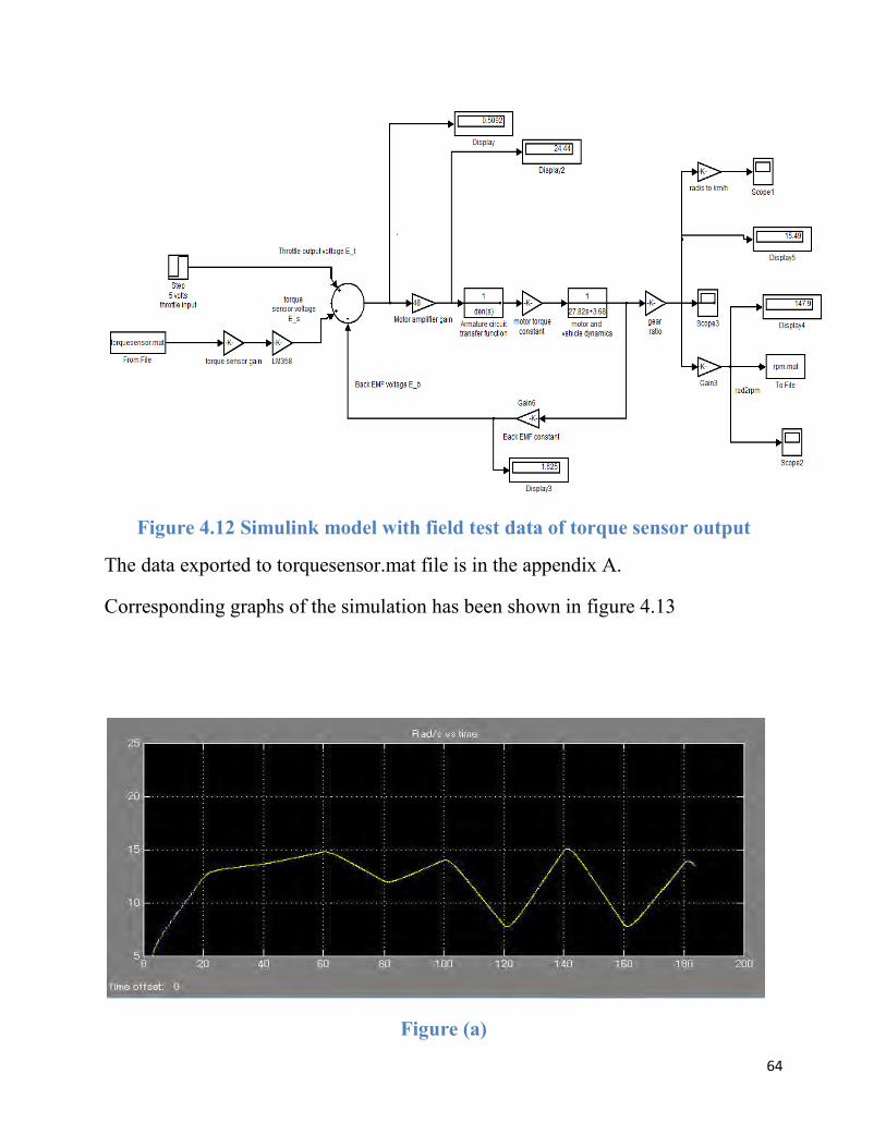
Figure 4.12 Simulink model with field test data of torque sensor output

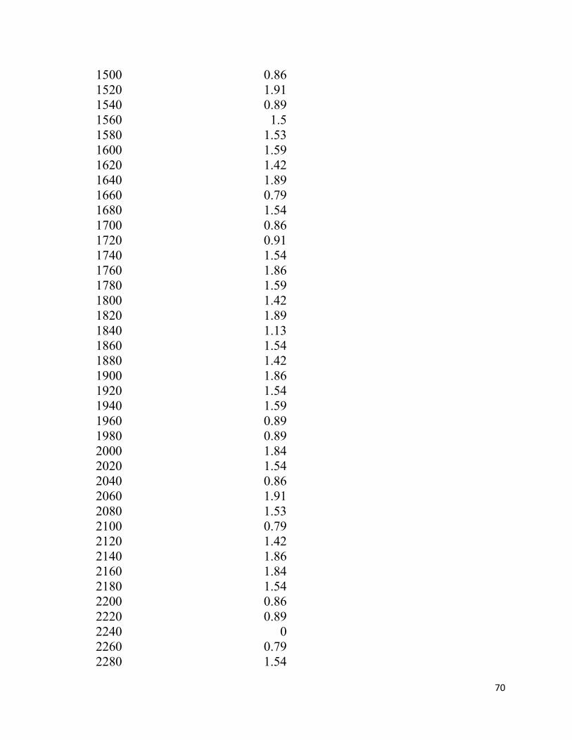
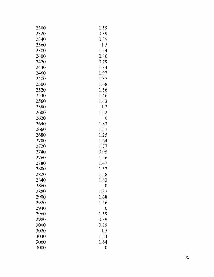
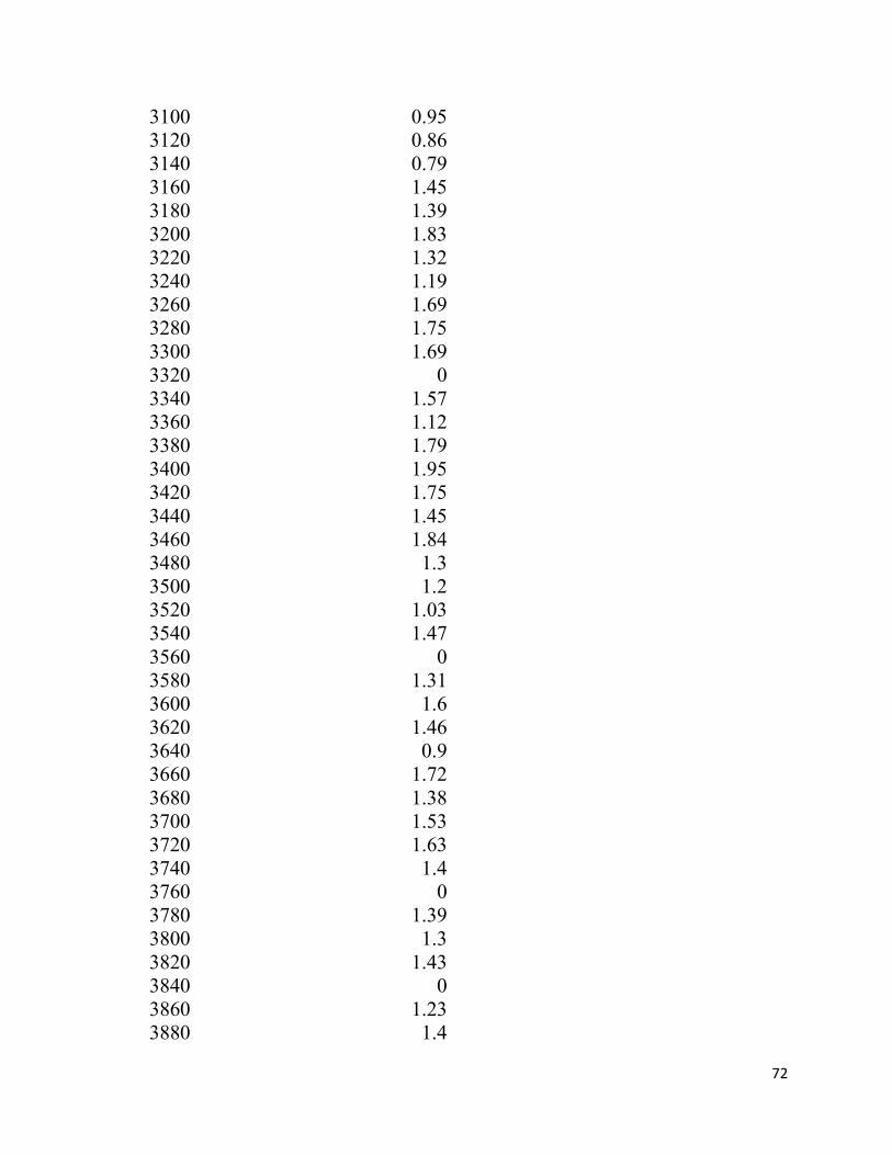
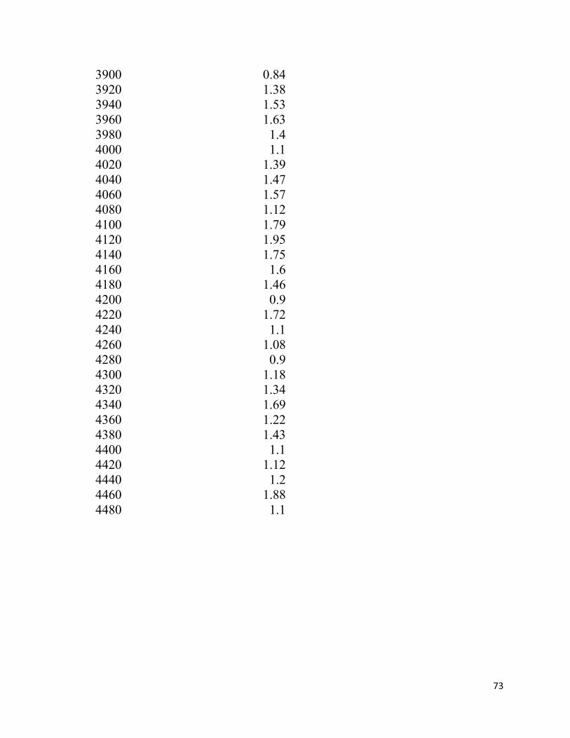
The data exported to torquesensor.mat file is in the appendix A.

Corresponding graphs of the simulation has been shown in fi

Simulink model with field test data of torque sensor output

The data exported to torquesensor.mat file is in the appendix A.

Corresponding graphs of the simulation has been shown in figure 4.13

Figure (a)

64

Simulink model with field test data of torque sensor output

gure 4.13

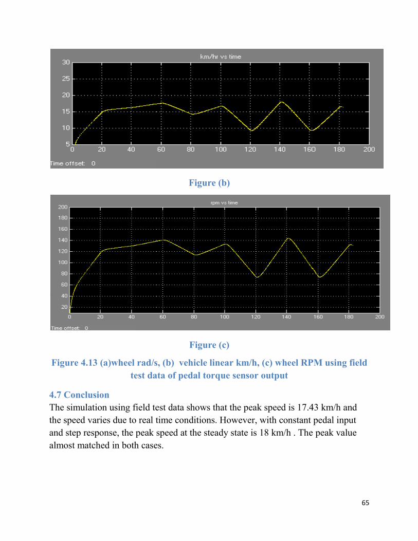
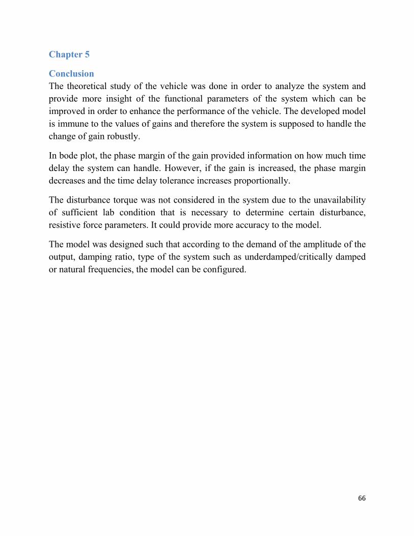
Figure 4.13 (a)wheel rad/s, (b) vehicle linear km/h, (c) wheel RPM using

test data of pedal torque sensor output

4.7 Conclusion

The simulation using field test data shows that the peak speed is 17.

the speed varies due to real time conditions. However, with constant pedal input

and step response, the peak speed at the steady state is 18 km/h . The peak value

almost matched in both cases.

Figure (b)

Figure (c)

(a)wheel rad/s, (b) vehicle linear km/h, (c) wheel RPM using

test data of pedal torque sensor output

The simulation using field test data shows that the peak speed is 17.43 km/h and



almost matched in both cases.

65

(a)wheel rad/s, (b) vehicle linear km/h, (c) wheel RPM using field

43 km/h and



66

Chapter 5

Conclusion

The theoretical study of the vehicle was done in order to analyze the system and

provide more insight of the functional parameters of the system which can be

improved in order to enhance the performance of the vehicle. The developed model

is immune to the values of gains and therefore the system is supposed to handle the

change of gain robustly.

In bode plot, the phase margin of the gain provided information on how much time

delay the system can handle. However, if the gain is increased, the phase margin

decreases and the time delay tolerance increases proportionally.

The disturbance torque was not considered in the system due to the unavailability

of sufficient lab condition that is necessary to determine certain disturbance,

resistive force parameters. It could provide more accuracy to the model.

The model was designed such that according to the demand of the amplitude of the

output, damping ratio, type of the system such as underdamped/critically damped

or natural frequencies, the model can be configured.

67

References

[1]N. Nise, Control systems engineering, 1st ed. Hoboken, NJ: Wiley, 2015.

[2]F. Khan, A. Aurony, A. Rahman, F. Munira, N. Halim and A. Azad, "Torque sensor based electrically

assisted hybrid rickshaw-van with PV assistance and solar battery charging station", Hdl.handle.net,

2015. [Online]. Available: http://hdl.handle.net/10361/6967. [Accessed: 09- Apr- 2017].

[3]R. Huq, N. Shuvo, P. Chakraborty and M. Hoque, "Development of Torque Sensor Based Electrically

Assisted Hybrid Rickshaw", Hdl.handle.net, 2012. [Online]. Available: http://hdl.handle.net/10361/2122.

[Accessed: 11- Apr- 2017].

[4]E. Cheever, "Electromechanical Systems", Lpsa.swarthmore.edu, 2015. [Online]. Available:

http://lpsa.swarthmore.edu/Systems/Electromechanical/SysElectMechSystems.html. [Accessed: 11-

Apr- 2017].

[5]C. Abagnale, M. Cardone, P. Iodice, S. Strano, M. Terzo and G. Vorraro, "Derivation and Validation of a

Mathematical Model for a Novel Electric Bicycle", 2015. [Online]. Available:

http://www.iaeng.org/publication/WCE2015/WCE2015_pp808-813.pdf. [Accessed: 11- Apr- 2017].

[6]2017. [Online]. Available:

https://en.nanotec.com/fileadmin/files/Katalog/Nanotec_Catalog_2017.pdf. [Accessed: 11- Apr- 2017].

[7]E. Cheever, "Elements of Rotating Mechanical Systems", Lpsa.swarthmore.edu, 2015. [Online].

Available: http://lpsa.swarthmore.edu/Systems/MechRotating/RotMechSysElem.html. [Accessed: 13-

Apr- 2017].

[8]E. Cheever, "Why make a root locus plot? - Erik Cheever", Lpsa.swarthmore.edu, 2015. [Online].

Available: http://lpsa.swarthmore.edu/Root_Locus/RootLocusWhy.html. [Accessed: 13- Apr- 2017].

[9] 2004. [Online]. Available: http://www.dartmouth.edu/~sullivan/22files/Bode_plots.pdf. [Accessed:

14- Apr- 2017].

[10]"Control Tutorials for MATLAB and Simulink - Introduction: Frequency Domain Methods for

Controller Design", Ctms.engin.umich.edu, 2017. [Online]. Available:

http://ctms.engin.umich.edu/CTMS/index.php?example=Introduction&section=ControlFrequency.

[Accessed: 14- Apr- 2017].

[11]S. Ayasun, U. Eminoğlu and Ş. Sönmez, "Computation of Stability Delay Margin of Time-Delayed

Generator Excitation Control System with a Stabilizing Transformer", 2014. .

68

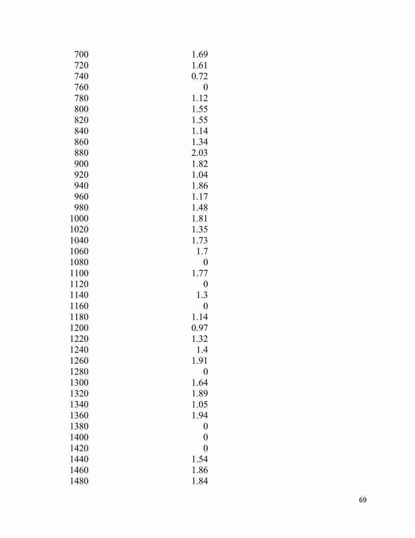
APPENDIX A

Table A : torque sensor input to the system with respect to time

Time (seconds)

Torque sensor input (voltage)

5 0 20 1.03 40 1.16 60 1.37 80 0.81

100 1.25 120 0 140 1.5 160 0 180 1.27 200 0 220 1.48 240 0 260 0 280 1.1 300 1.22 320 1.71 340 0 360 1.53 380 1.14 400 1.5 420 0.66 440 1.97 460 0 480 0.97 500 1.27 520 0 540 1.17 560 1.59 580 1.51 600 1.15 620 1.68 640 1.8 660 1.7 680 1.32

69

700 1.69 720 1.61 740 0.72 760 0 780 1.12 800 1.55 820 1.55 840 1.14 860 1.34 880 2.03 900 1.82 920 1.04 940 1.86 960 1.17 980 1.48

1000 1.81 1020 1.35 1040 1.73 1060 1.7 1080 0 1100 1.77 1120 0 1140 1.3 1160 0 1180 1.14 1200 0.97 1220 1.32 1240 1.4 1260 1.91 1280 0 1300 1.64 1320 1.89 1340 1.05 1360 1.94 1380 0 1400 0 1420 0 1440 1.54 1460 1.86 1480 1.84

70

1500 0.86 1520 1.91 1540 0.89 1560 1.5 1580 1.53 1600 1.59 1620 1.42 1640 1.89 1660 0.79 1680 1.54 1700 0.86 1720 0.91 1740 1.54 1760 1.86 1780 1.59 1800 1.42 1820 1.89 1840 1.13 1860 1.54 1880 1.42 1900 1.86 1920 1.54 1940 1.59 1960 0.89 1980 0.89 2000 1.84 2020 1.54 2040 0.86 2060 1.91 2080 1.53 2100 0.79 2120 1.42 2140 1.86 2160 1.84 2180 1.54 2200 0.86 2220 0.89 2240 0 2260 0.79 2280 1.54

71

2300 1.59 2320 0.89 2340 0.89 2360 1.5 2380 1.54 2400 0.86 2420 0.79 2440 1.84 2460 1.97 2480 1.37 2500 1.68 2520 1.56 2540 1.46 2560 1.43 2580 1.2 2600 1.52 2620 0 2640 1.83 2660 1.57 2680 1.25 2700 1.64 2720 1.77 2740 0.95 2760 1.56 2780 1.47 2800 1.52 2820 1.58 2840 1.83 2860 0 2880 1.37 2900 1.68 2920 1.56 2940 0 2960 1.59 2980 0.89 3000 0.89 3020 1.5 3040 1.54 3060 1.64 3080 0

72

3100 0.95 3120 0.86 3140 0.79 3160 1.45 3180 1.39 3200 1.83 3220 1.32 3240 1.19 3260 1.69 3280 1.75 3300 1.69 3320 0 3340 1.57 3360 1.12 3380 1.79 3400 1.95 3420 1.75 3440 1.45 3460 1.84 3480 1.3 3500 1.2 3520 1.03 3540 1.47 3560 0 3580 1.31 3600 1.6 3620 1.46 3640 0.9 3660 1.72 3680 1.38 3700 1.53 3720 1.63 3740 1.4 3760 0 3780 1.39 3800 1.3 3820 1.43 3840 0 3860 1.23 3880 1.4

73

3900 0.84 3920 1.38 3940 1.53 3960 1.63 3980 1.4 4000 1.1 4020 1.39 4040 1.47 4060 1.57 4080 1.12 4100 1.79 4120 1.95 4140 1.75 4160 1.6 4180 1.46 4200 0.9 4220 1.72 4240 1.1 4260 1.08 4280 0.9 4300 1.18 4320 1.34 4340 1.69 4360 1.22 4380 1.43 4400 1.1 4420 1.12 4440 1.2 4460 1.88 4480 1.1

hematical Model and Stability Analysis of Electric Vehicle

Documents