Helsinki University of Technology Systems Analysis Laboratory RICHER – A Method for Exploiting RICHER – A Method for Exploiting Incomplete Ordinal Information in Incomplete Ordinal Information in Value Trees Value Trees Antti Punkka and Ahti Salo Systems Analysis Laboratory Helsinki University of Technology P.O. Box 1100, 02015 HUT, Finland [email protected] http://www.sal.hut.fi/

Helsinki University of Technology Systems Analysis Laboratory RICHER – A Method for Exploiting Incomplete Ordinal Information in Value Trees Antti Punkka.
Dec 17, 2015
Welcome message from author
This document is posted to help you gain knowledge. Please leave a comment to let me know what you think about it! Share it to your friends and learn new things together.
Transcript

Helsinki University of Technology Systems Analysis Laboratory
RICHER – A Method for Exploiting Incomplete RICHER – A Method for Exploiting Incomplete Ordinal Information in Value TreesOrdinal Information in Value Trees
Antti Punkka and Ahti Salo
Systems Analysis Laboratory
Helsinki University of Technology
P.O. Box 1100, 02015 HUT, Finland
http://www.sal.hut.fi/
Helsinki University of Technology Systems Analysis Laboratory
2
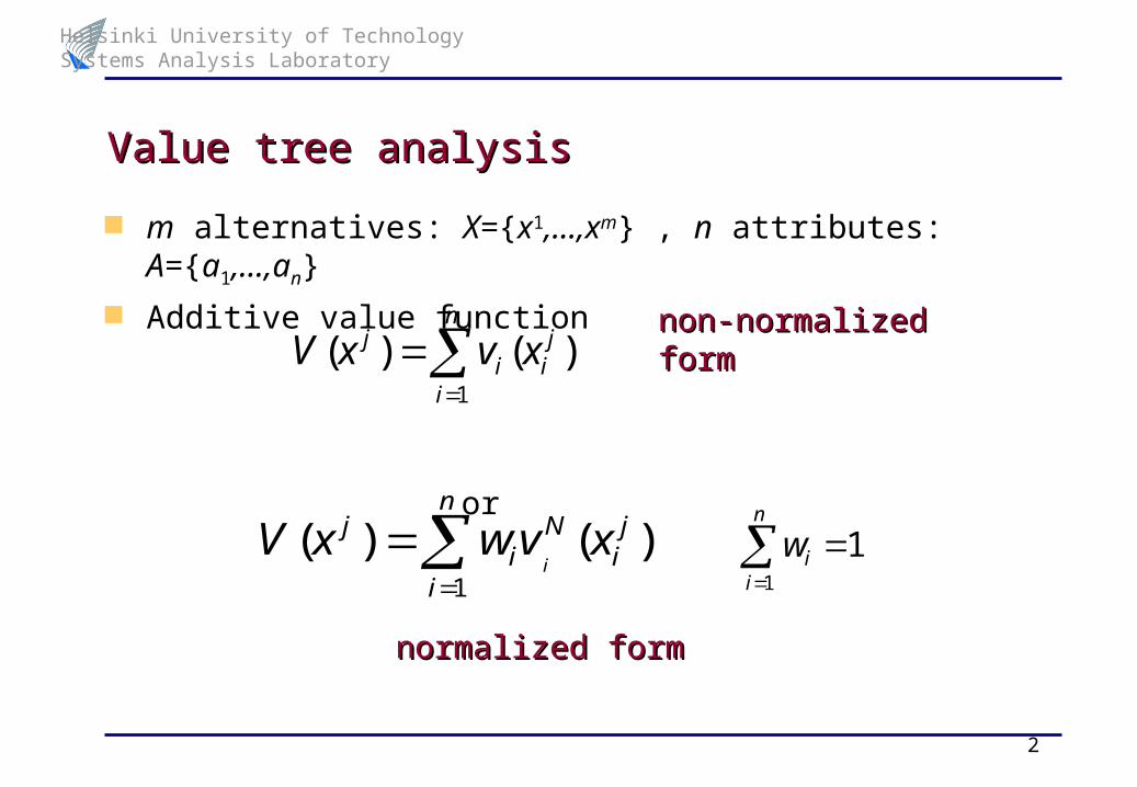
m alternatives: X={x1,…,xm} , n attributes: A={a1,…,an} Additive value function
or
Value tree analysisValue tree analysis
n
i
jii
j xvxV1
)()(
n
i
ji
Ni
j xvwxVi
1
)()(
n
iiw
1
1
non-normalized formnon-normalized form
normalized formnormalized form
Helsinki University of Technology Systems Analysis Laboratory
3
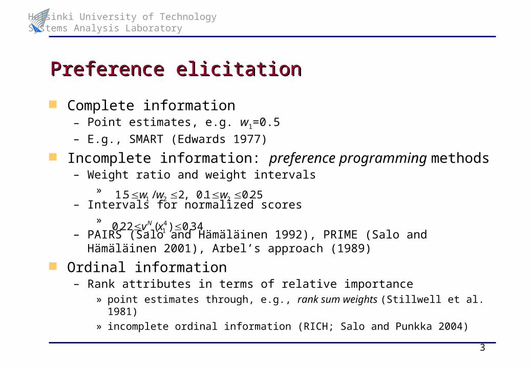
Preference elicitation Preference elicitation
Complete information– Point estimates, e.g. w1=0.5
– E.g., SMART (Edwards 1977)
Incomplete information: preference programming methods– Weight ratio and weight intervals
»
– Intervals for normalized scores»
– PAIRS (Salo and Hämäläinen 1992), PRIME (Salo and Hämäläinen 2001), Arbel’s approach (1989)
Ordinal information– Rank attributes in terms of relative importance
» point estimates through, e.g., rank sum weights (Stillwell et al. 1981)» incomplete ordinal information (RICH; Salo and Punkka 2004)
25.01.0,2/5.1 221 www
34.0)(22.0 411
xvN
Helsinki University of Technology Systems Analysis Laboratory
4
Incomplete preference informationIncomplete preference information
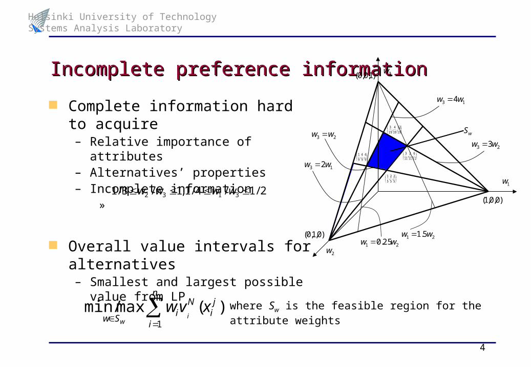
Complete information hard to acquire – Relative importance of attributes– Alternatives’ properties– Incomplete information
»
Overall value intervals for alternatives– Smallest and largest possible value from
LP
n
i
ji
Ni
Swxvw
iw 1
)(maxmin/ where Sw is the feasible region for the attribute weights
3w
2w
1w
wS23 ww
)0,1,0(
)1,0,0(
)0,0,1(
23 3ww
13 2ww
13 4ww
9
4,
9
4,
9
1
5
2,
5
2,
5
1
11
6,
11
2,
11
3
19
12,
19
4,
19
3
21 5.1 ww 21 25.0 ww
2/1/4/1,1/3/1 3132 wwww
Helsinki University of Technology Systems Analysis Laboratory
5
Pairwise dominance relationPairwise dominance relation
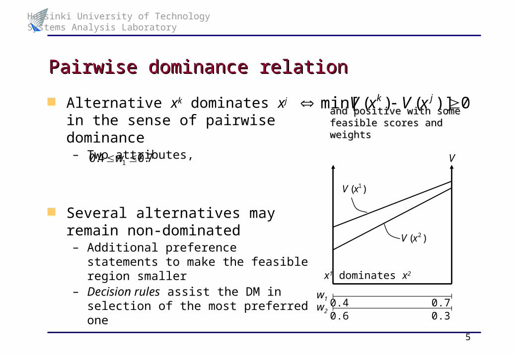
Alternative xk dominates xj in the sense of pairwise dominance– Two attributes,
Several alternatives may remain non-dominated– Additional preference statements to make
the feasible region smaller– Decision rules assist the DM in selection
of the most preferred one
0)]()(min[ jk xVxV
V
w1 0.4 0.7w20.6 0.3
x1 dominates x2
)( 1xV
)( 2xV
7.04.0 1 w
and positive with some and positive with some feasible scores and weightsfeasible scores and weights

Helsinki University of Technology Systems Analysis Laboratory
6
Incomplete ordinal preference informationIncomplete ordinal preference information
Complete ordinal information is a complete rank-ordering of attributes or alternatives– Rankings are exactly known for each alternative– Leads to a convex set of feasible scores and weights, when interpreted as
incomplete preference information
The RICH (Rank Inclusion in Criteria Hierarchies) method– Incomplete ordinal statements about relative importance of attributes– ”Cost is the most important attribute”– ”Environmental factors is among the three most important attributes”– Several rank-orderings can be compatible with the preference statements
» e.g.: either attribute a1 or a2 is the most important of the three attributes aa33 is either the second or the least important one is either the second or the least important one
» may lead to non-convex feasible region of the attribute weights

Helsinki University of Technology Systems Analysis Laboratory
7
Non-convex feasible region in RICHNon-convex feasible region in RICH ”Either a1 or a2 is the most
important of the three attributes”
Calculation by dividing into compatible rank-orderings
– Extreme points readily computed– Lower bounds for weights wi b 0
Full support provided by RICH Decisions ©, http://www.decisionarium.hut.fi/
– Applications» evalution of risk management tools
(Ojanen et al. 2004)» support for setting priorities for a
research programme in wood material science (Salo and Liesiö 2004)
3w
2w
1w
)3,2,1(r)0,0,1(
)0,1,0(
)1,0,0(
23 ww
13 ww
)3,1,2(r
)1,3,2(r
)2,3,1(r

Helsinki University of Technology Systems Analysis Laboratory
8
The RICHER (RICH with Extended Rankings) methodThe RICHER (RICH with Extended Rankings) method
Extends incomplete ordinal information to alternatives– ”Alternatives x1, x2 and x3 are the three most preferred with regard to
environmental factors”– ”Alternative x1 is not among the three most preferred ones”– ”Considering alternatives x1, x2 and x3, the least preferred with regard to
cost is x1”
Statements about attribute weights incorporated as well
Comparison to the RICH method– Suitable also for statements about alternatives– Computationally much more efficient– Includes all features of RICH– Allows evaluation within subsets– Applicable in conjunction with other preference programming methods

Helsinki University of Technology Systems Analysis Laboratory
9
Modeling of incomplete ordinal information (1/4)Modeling of incomplete ordinal information (1/4)
Rank-ordering –function r– Bijection from (sub)set of alternatives X’X (or (sub)set of attributes) to set of
rankings– E.g., r=(r(x1), r(x2), r(x3))=(1,3,2)
– The smaller the ranking, the better the alternative
» e.g., ”r(x4)=1 the ranking of x4 is 1, i.e. it is the most preferred”
– Several rank-orderings may be compatible with the preference information
– Incomplete ordinal statements about alternatives can be expressed with regard to different sets of attributes A’
» single attribute, (sub)set of attributes or holistic statements considering all attributes
» e.g., one can subject statements to cost and environmental factors together
)()()()( kjkj xvxvxrxr

Helsinki University of Technology Systems Analysis Laboratory
10
Modeling of incomplete ordinal information (2/4)Modeling of incomplete ordinal information (2/4)
Non-normalized form of value function
Set of feasible values V includes score vectors v=(v(x1),..., v(xm)) – v(xk) denotes the value of xk with regard to some set of attributes
» e.g., if A’={a2}, then v(xk)=v2(x2k)
» e.g., if A’=A, then v(xk)=V(xk)
– Restricted by preference statements
Feasible region associated with a rank-ordering is convex
}',),()(if)()(|{)( ' XxxxrxrxvxvvrS jkjkjkX V
n
i
jii
j xvxV1
)()(

Helsinki University of Technology Systems Analysis Laboratory
11
Modeling of incomplete ordinal information (3/4)Modeling of incomplete ordinal information (3/4)
Elicitation of the preference statements is carried out through an alternative set IX’X and a ranking set J{1,...,m’}, where m’=|X’|
– If |I||J|, the rankings in J are attained by alternatives in I– If |I|<|J|, the alternatives in I have their rankings in J– Sets subjected to X’ and A’ denoted by I(A’,X’) and J(A’,X’)
Examples
– x1 and x2 are among the three most preferred ones with regard to cost attribute a1. Now A’={a1} and X’=X, I({a1}; X)={x1,x2}, J({a1}; X)={1,2,3}
– Holistically (A’=A) the two least preferred are among x4,x5, x8,x9: I(A; X)= {x4,x5, x8,x9}, J(A; X)={m-1,m}
– Holistically the most preferred of the set X’={x1, x2, x7} is x1: I(A; X’)={x1}, J(A; X’)={1}

Helsinki University of Technology Systems Analysis Laboratory
12
Modeling of incomplete ordinal information (4/4)Modeling of incomplete ordinal information (4/4)
Sets I and J lead to compatible rank-orderings R(I,J)
The feasible region associated with many compatible rank-orderings is usually non-convex
Statements can be given with regard to different attribute sets– Several rank-orderings may be compatible with each of these sets
)(),(),(rSJIS
JIRr

Helsinki University of Technology Systems Analysis Laboratory
13
Mixed integer linear programming model (1/5)Mixed integer linear programming model (1/5)
Overcoming the non-convexity
– Continuous ”milestone variable” zk distinguishes between the values of alternatives with rankings k and k+1
– If xj’s ranking is at most k, its value is at least zk and we let yk(xj)=1, else 0
– There are exactly k alternatives whose ranking is at most k» e.g., the three rankings 1, 2 and 3 are at most 3
1r 2r 4r3r 5r
12 y
1z 2z 3z 4z 5z
6r
03 y

Helsinki University of Technology Systems Analysis Laboratory
14
Mixed integer linear programming modelMixed integer linear programming model (2/5) (2/5)
Formally
For the sake of interpretational and computational matters, we set
'
1',...,1,)(
0,',1',...,1
)()())(1()(
Xx
jk
j
jkk
j
jk
jk
j
mkkxy
MXxmk
MxyzxvMxyxvz
',1',...,2),()( 1 Xxmkxyxy jjk
jk
Helsinki University of Technology Systems Analysis Laboratory
15
Mixed integer linear programming modelMixed integer linear programming model (3/5) (3/5)
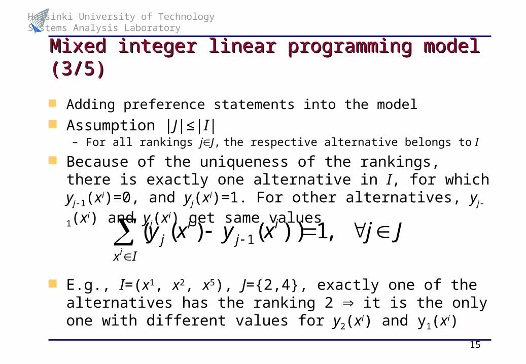
Adding preference statements into the model Assumption |J|≤|I|
– For all rankings jJ, the respective alternative belongs to I
Because of the uniqueness of the rankings, there is exactly one alternative in I, for which yj-1(xi)=0, and yj(xi)=1. For other alternatives, yj-1(xi) and yj(xi) get same values
E.g., I=(x1, x2, x5), J={2,4}, exactly one of the alternatives has the ranking 2 it is the only one with different values for y2(xi) and y1(xi)
Jjxyxy ij
ij
Ixi
,1))()(( 1

Helsinki University of Technology Systems Analysis Laboratory
16
Mixed integer linear programming modelMixed integer linear programming model (4/5) (4/5)
Some milestone and binary variables and the respective constraints are redundant– Given a statement that alternatives x1 and x2 are the two most preferred,
for example variables z1, z3 and y1(xj), y3(xj) are not needed
» actually only z2 and y2(xj) are needed
If set J is ”sequential”, i.e., it constitutes of consecutive positive integers, the number of variables and constraints can be substantially decreased– For example sets {3,4,5} and {1} are sequential, set {1,3} not
For the compatible rank-orderings associated with sets I and J, |I||J|, it holds
k
i
k
iii JJJIRJIR
1 1
),,(),(
Helsinki University of Technology Systems Analysis Laboratory
17
Mixed integer linear programming modelMixed integer linear programming model (5/5) (5/5)
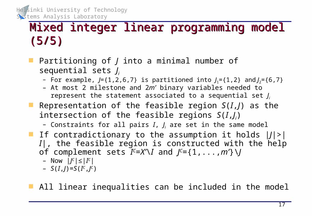
Partitioning of J into a minimal number of sequential sets Ji– For example, J={1,2,6,7} is partitioned into J1={1,2} and J2={6,7}– At most 2 milestone and 2m’ binary variables needed to represent the
statement associated to a sequential set Ji
Representation of the feasible region S(I,J) as the intersection of the feasible regions S(I,Ji)– Constraints for all pairs I, Ji are set in the same model
If contradictionary to the assumption it holds |J|>|I|, the feasible region is constructed with the help of complement sets IC=X’\I and JC={1,...,m’}\J– Now |JC|≤|IC|– S(I,J)=S(IC,JC)
All linear inequalities can be included in the model
Helsinki University of Technology Systems Analysis Laboratory
18
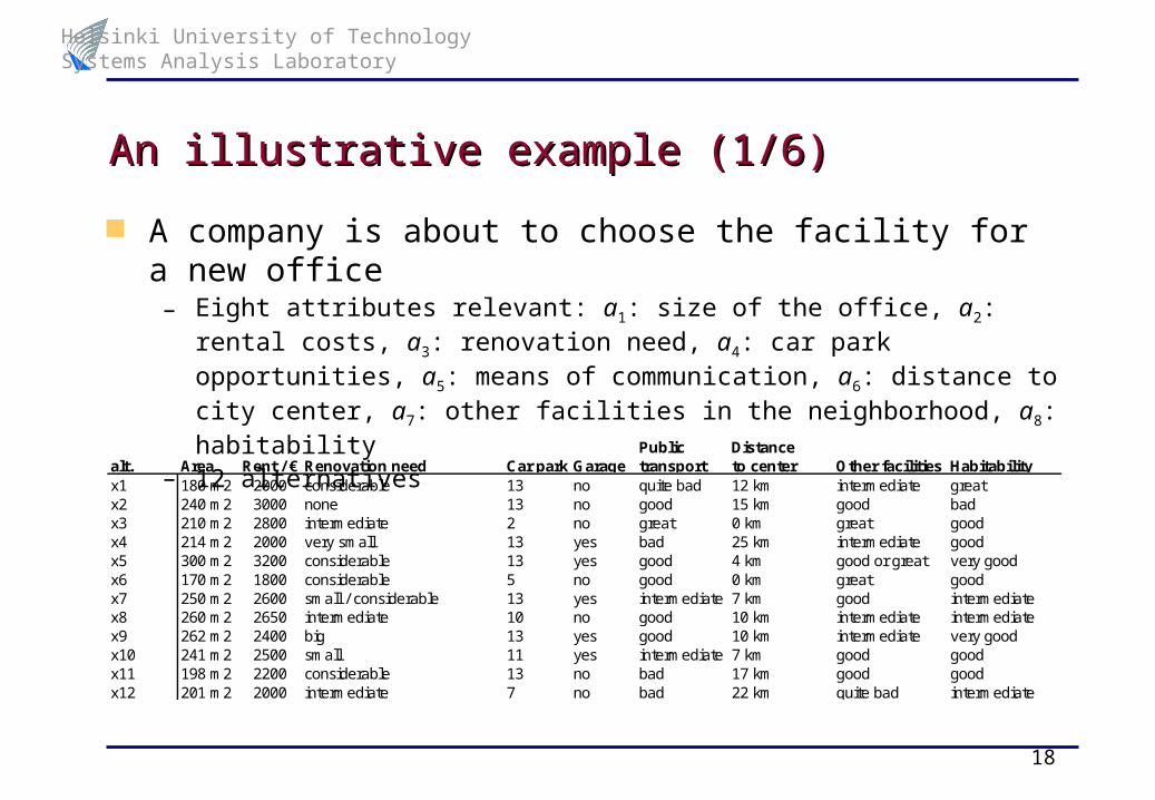
An illustrative example (1/6)An illustrative example (1/6)
A company is about to choose the facility for a new office– Eight attributes relevant: a1: size of the office, a2: rental costs, a3: renovation
need, a4: car park opportunities, a5: means of communication, a6: distance to city center, a7: other facilities in the neighborhood, a8: habitability
– 12 alternatives
Public Distancealt. Area Rent / € Renovation need Car park Garage transport to center Other facilities Habitabilityx1 180 m2 2000 considerable 13 no quite bad 12 km intermediate greatx2 240 m2 3000 none 13 no good 15 km good badx3 210 m2 2800 intermediate 2 no great 0 km great goodx4 214 m2 2000 very small 13 yes bad 25 km intermediate goodx5 300 m2 3200 considerable 13 yes good 4 km good or great very goodx6 170 m2 1800 considerable 5 no good 0 km great goodx7 250 m2 2600 small / considerable 13 yes intermediate 7 km good intermediatex8 260 m2 2650 intermediate 10 no good 10 km intermediate intermediatex9 262 m2 2400 big 13 yes good 10 km intermediate very goodx10 241 m2 2500 small 11 yes intermediate 7 km good goodx11 198 m2 2200 considerable 13 no bad 17 km good goodx12 201 m2 2000 intermediate 7 no bad 22 km quite bad intermediate
Helsinki University of Technology Systems Analysis Laboratory
19
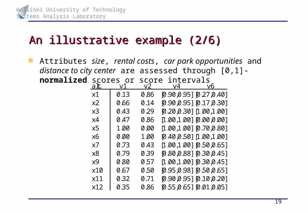
An illustrative example (2/6)An illustrative example (2/6)
Attributes size, rental costs, car park opportunities and distance to city center are assessed through [0,1]-normalized scores or score intervals
alt. v1 v2 v4 v6x1 0.13 0.86 [0.90,0.95] [0.27,0.40]x2 0.66 0.14 [0.90,0.95] [0.17,0.30]x3 0.43 0.29 [0.20,0.30] [1.00,1.00]x4 0.47 0.86 [1.00,1.00] [0.00,0.00]x5 1.00 0.00 [1.00,1.00] [0.70,0.80]x6 0.00 1.00 [0.40,0.50] [1.00,1.00]x7 0.73 0.43 [1.00,1.00] [0.50,0.65]x8 0.79 0.39 [0.80,0.88] [0.30,0.45]x9 0.80 0.57 [1.00,1.00] [0.30,0.45]x10 0.67 0.50 [0.95,0.98] [0.50,0.65]x11 0.32 0.71 [0.90,0.95] [0.10,0.20]x12 0.35 0.86 [0.55,0.65] [0.01,0.05]

Helsinki University of Technology Systems Analysis Laboratory
20
An illustrative example (3/6)An illustrative example (3/6)
Other information is turned into incomplete ordinal statements– E.g., alternative x2 is the only one with no renovation need (a3), hence the ranking 1
– E.g., alternative x2 is the least preferred w.r.t. habitability (a8)
attr. I J attr. I Ja3 {x2} {1} a7 {x3,x6} {1,2,3}
{x4} {2} {x5} {1,2,3,4,5,6,7}{x10} {3,4} {x2,x7,x10,x11} {3,4,5,6,7}{x7} {3,4,8,9,10,11,12} {x1,x4,x8,x9} {8,9,10,11}{x3,x8,x12} {4,5,6,7} {x12} {12}{x9} {7,8}{x1,x5,x6,x11} {8,9,10,11,12}
a5 {x3} {1} a8 {x1} {1}{x2,x5,x6,x8,x9} {2,3,4,5,6} {x5,x9} {2,3}{x7,x10} {7,8} {x3,x4,x6,x10,x11} {4,5,6,7,8}{x1} {9} {x7,x8,x12} {9,10,11}{x4,x11,x12} {10,11,12} {x2} {12}

Helsinki University of Technology Systems Analysis Laboratory
21
An illustrative example (4/6)An illustrative example (4/6)
Information on attributes’ relative importance– Complete rank-ordering of the attributes is r(a1,a2,...,a8)=(1,2,...,8)
– A weight of 0.50 is assigned to the most important attribute, size of the office– Weights are lower bounded by wi 1/3n
A holistic preference for x4 over x1 over x3
)()()( 314 xVxVxV
24
1...50.0 821 www

Helsinki University of Technology Systems Analysis Laboratory
22
An illustrative example (5/6)An illustrative example (5/6)
Pairwise bounds (minima of overall value differences) indicate that there are 5 non-dominated alternatives x5, x7, x8, x9 and x10
alternative xx1 x2 x3 x4 x5 x6 x7 x8 x9 x10 x11 x12
PB(x1,x) - -0.263 0.000 -0.282 -0.428 -0.058 -0.350 -0.354 -0.323 -0.368 -0.089 -0.153PB(x2,x) 0.033 - 0.033 -0.123 -0.312 -0.025 -0.171 -0.178 -0.274 -0.199 -0.056 -0.048PB(x3,x) -0.040 -0.263 - -0.282 -0.428 -0.058 -0.350 -0.354 -0.323 -0.368 -0.089 -0.153PB(x4,x) 0.000 -0.244 0.000 - -0.376 0.007 -0.229 -0.236 -0.314 -0.264 -0.071 0.004PB(x5,x) 0.143 0.049 0.143 0.029 - 0.137 -0.051 -0.061 -0.155 -0.038 0.105 0.102PB(x6,x) -0.238 -0.390 -0.238 -0.397 -0.655 - -0.464 -0.481 -0.561 -0.482 -0.308 -0.263PB(x7,x) 0.076 -0.043 0.076 -0.079 -0.309 0.058 - -0.137 -0.217 -0.150 0.016 0.035PB(x8,x) 0.119 -0.089 0.119 -0.115 -0.215 0.103 -0.177 - -0.188 -0.192 0.067 0.039PB(x9,x) 0.172 -0.042 0.172 -0.028 -0.173 0.203 -0.129 -0.135 - -0.106 0.167 0.087PB(x10,x) 0.143 -0.070 0.143 -0.099 -0.239 0.085 -0.158 -0.067 -0.164 - 0.054 0.102PB(x11,x) -0.152 -0.298 -0.152 -0.310 -0.569 -0.150 -0.382 -0.388 -0.465 -0.399 - -0.183PB(x12,x) -0.115 -0.349 -0.115 -0.361 -0.480 -0.079 -0.433 -0.439 -0.418 -0.452 -0.177 -
Helsinki University of Technology Systems Analysis Laboratory
23
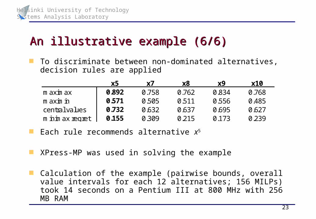
An illustrative example (6/6)An illustrative example (6/6)
To discriminate between non-dominated alternatives, decision rules are applied
Each rule recommends alternative x5
XPress-MP was used in solving the example
Calculation of the example (pairwise bounds, overall value intervals for each 12 alternatives; 156 MILPs) took 14 seconds on a Pentium III at 800 MHz with 256 MB RAM
x5 x7 x8 x9 x10maximax 0.892 0.758 0.762 0.834 0.768maximin 0.571 0.505 0.511 0.556 0.485central values 0.732 0.632 0.637 0.695 0.627minimax regret 0.155 0.309 0.215 0.173 0.239

Helsinki University of Technology Systems Analysis Laboratory
24
ConclusionConclusion
The DM can give incomplete ordinal information about the alternatives with regard to a single attribute, a set of attributes or holistically
Statements about relative importance of attributes are allowed, as well
Based on a linear model and hence it can be used in conjunction with other preference programming methods
Computationally far more efficient than RICH, and more flexible as it contains all features of RICH
Software implementation of RICHER Decisions © ongoing
Future research directions – Modeling of classification procedures with RICHER methodology (cf. the example in this
presentation)– Application of RICHER methodology to voting or other group decision processes– Application of incompelete ordinal information in Robust Portfolio Modeling (RPM)

Helsinki University of Technology Systems Analysis Laboratory
25
Related referencesRelated referencesArbel, A., “Approximate Articulation of Preference and Priority DerivationApproximate Articulation of Preference and
Priority Derivation”, European Journal of Operations Research 43 (1989) 317-326.
Edwards, W., “How to Use Multiattribute Utility Measurement for Social Decision Making”, IEEE Transactions on Systems,
Man, and Cybernetics 7 (1977) 326-340.
Ojanen, O., Makkonen, S. and Salo, A., “A Multi-Criteria Framework for the Selection of Risk Analysis Methods at Energy
Utilities”, International Journal of Risk Assessment and Management (to appear).
Salo, A. ja R. P. Hämäläinen, "Preference Assessment by Imprecise Ratio Statements”, Operations Research 40 (1992)
1053-1061.
Salo, A. and Hämäläinen, R. P., “Preference Ratios in Multiattribute Evaluation (PRIME) - Elicitation and Decision
Procedures under Incomplete Information”, IEEE Transactions on Systems, Man, and Cybernetics 31 (2001) 533-
545.
Salo, A. and Liesiö, J., “A Case Study in Participatory Priority-Setting for a Scandinavian Research Programme”,
submitted manuscript.
Salo, A. and Punkka, A., “Rank Inclusion in Criteria Hierarchies”, European Journal of Operations Research (to appear).
Stillwell, W. G., Seaver, D. A. and Edwards, W., “A Comparison of Weight Approximation Techniques in Multiattribute
Utility Decision Making”, Organizational Behavior and Human Performance 28 (1981) 62-77.
Related Documents