DIFFERENTIAL AND INTEGRAL CALCULUS, I LECTURE NOTES (TEL AVIV UNIVERSITY, FALL 2009) Contents Preliminaries i Preparatory reading i Reading i Problem books i Basic notation ii Basic Greek letters iv 1. Real Numbers 1 1.1. Infinite decimal strings 1 1.2. The axioms 1 1.3. Application: solution of equation s n = a 5 1.4. The distance on R 6 2. Upper and lower bounds 8 2.1. Maximum/minimum supremum/infimum 8 2.2. Some corollaries: 10 3. Three basic lemmas: Cantor, Heine-Borel, Bolzano-Weierstrass 12 3.1. The nested intervals principle 12 3.2. The finite subcovering principle 13 3.3. The accumulation principle. 13 3.4. Appendix: Countable and uncountable subsets of R 14 4. Sequences and their limits 18 4.1. 18 4.2. Fundamental properties of the limits 19 5. Convergent sequences 22 5.1. Examples 22 5.2. Two theorems 23 5.3. More examples 25 6. Cauchy’s sequences. Upper and lower limits. Extended convergence 28 6.1. Cauchy’s sequences 28 6.2. Upper and lower limits 29 6.3. Convergence in wide sense 31 7. Subsequences and partial limits. 33 Date : 29 October, 2009. 1

Welcome message from author
This document is posted to help you gain knowledge. Please leave a comment to let me know what you think about it! Share it to your friends and learn new things together.
Transcript

DIFFERENTIAL AND INTEGRAL CALCULUS, I
LECTURE NOTES (TEL AVIV UNIVERSITY, FALL 2009)
Contents
Preliminaries iPreparatory reading iReading iProblem books iBasic notation iiBasic Greek letters iv1. Real Numbers 11.1. Infinite decimal strings 11.2. The axioms 11.3. Application: solution of equation sn = a 51.4. The distance on R 62. Upper and lower bounds 82.1. Maximum/minimum supremum/infimum 82.2. Some corollaries: 103. Three basic lemmas:
Cantor, Heine-Borel, Bolzano-Weierstrass 123.1. The nested intervals principle 123.2. The finite subcovering principle 133.3. The accumulation principle. 133.4. Appendix: Countable and uncountable subsets of R 144. Sequences and their limits 184.1. 184.2. Fundamental properties of the limits 195. Convergent sequences 225.1. Examples 225.2. Two theorems 235.3. More examples 256. Cauchy’s sequences. Upper and lower limits.
Extended convergence 286.1. Cauchy’s sequences 286.2. Upper and lower limits 296.3. Convergence in wide sense 317. Subsequences and partial limits. 33
Date: 29 October, 2009.
1

2 LECTURE NOTES (TEL AVIV, 2009)
7.1. Subsequences 337.2. Partial limits 338. Infinite series 368.1. 368.2. Examples 368.3. Cauchy’s criterion for convergence. Absolute convergence 388.4. Series with positive terms. Convergence tests 389. Rearrangement of the infinite series 429.1. Be careful! 429.2. Rearrangement of the series 429.3. Rearrangement of conditionally convergent series 4310. Limits of functions. Basic properties 4610.1. Cauchy’s definition of limit 4610.2. Heine’s definition of limit 4710.3. Limits and arithmetic operations 48
10.4. The first remarkable limit: limx→0
sinx
x= 1 49
10.5. Limits at infinity and infinite limits 5110.6. Limits of monotonic functions 5211. The exponential function and the logarithm 5311.1. The function t 7→ at. 5311.2. The logarithmic function loga x. 5512. The second remarkable limit.
The symbols “o small” and “∼” 58
12.1. limx→±∞
(1 +
1x
)x
= e 58
12.2. Infinitesimally small values and the symbols o and ∼. 5813. Continuous functions, I 6113.1. Continuity 6113.2. Points of discontinuity 6113.3. Local properties of continuous functions 6314. Continuous functions, II 6614.1. Global properties of continuous functions 6614.2. Uniform continuity 6814.3. Inverse functions 7015. The derivative 7215.1. Definition and some examples 7215.2. Some rules 7415.3. Derivative of the inverse function and of the composition 7516. Applications of the derivative 7816.1. Local linear approximation. 7816.2. The tangent line 7916.3. Lagrange interpolation. 8017. Derivatives of higher orders 8317.1. Definition and examples 83

DIFFERENTIAL AND INTEGRAL CALCULUS, I 3
17.2. The Leibniz rule. 8618. Basic theorems of the differential calculus:
Fermat, Rolle, Lagrange 8818.1. Theorems of Fermat and Rolle. Local extrema 8818.2. Mean-value theorems 9219. Applications of fundamental theorems 9619.1. L’Hospital’s rule 9619.2. Appendix: Algebraic numbers 9820. Inequalities 10120.1. 2
πx ≤ sinx ≤ x, 0 ≤ x ≤ π2 101
20.2. x1+x < log(1 + x) < x, x > −1, x 6= 0 101
20.3. Bernoulli’s inequalities 10220.4. Young’s inequality 10320.5. Holder’s inequality 10420.6. Minkowski’s inequality 10521. Convex functions. Jensen’s inequality 10721.1. Definition 10721.2. Fundamental properties of convex functions 10921.3. 11021.4. Jensen’s inequality 11122. The Taylor expansion 11322.1. Local polynomial approximation. Peano’s theorem 11322.2. The Taylor remainder. Theorems of Lagrange and Cauchy 11423. Taylor expansions of elementary functions 11723.1. The exponential function 11723.2. The sine and cosine functions 11823.3. The logarithmic function 11923.4. The binomial series 12023.5. The Taylor series for arctanx 12123.6. Some computations 12223.7. Application to the limits 12324. The complex numbers 12424.1. Basic definitions and arithmetics 12424.2. Geometric representation of complex numbers. The argument 12524.3. Convergence in C 12725. The fundamental theorem of algebra and its corollaries 12825.1. The theorem and its proof 12825.2. Factoring the polynomials 12925.3. Rational functions. Partial fraction decomposition 13026. Complex exponential function 13326.1. Absolutely convergent series 13326.2. The complex exponent 134

DIFFERENTIAL AND INTEGRAL CALCULUS, I i
Preliminaries
Preparatory reading. These books are intended for high-school students who likemath. All three books are great, my personal favorite is the first one.
(1) R. Courant, H. Robbins, I. Stewart, What is mathematics, Oxford, 1996 (orearlier editions).
(2) T. W. Korner, The pleasures of counting, Cambridge U. Press, 1996.(3) K. M. Ball, Strange curves, counting rabbits, and other mathematical explo-
rations, Princeton University Press, 2003.
Reading. There are many good textbooks in analysis, though I am not going to followany of them too closely. The following list reflects my personal taste:
(1) V. A. Zorich, Mathematical analysis, vol.1, Springer, 2004.(2) A. Browder, Mathematical analysis. An introduction. Undergraduate Texts in
Mathematics. Springer-Verlag, New York, 1996.(3) R. Courant and F. John, Introduction to calculus and analysis, vol.1, Springer,
1989 (or earlier editions).(4) D. Maizler, Infinitesimal calculus (in Hebrew).(5) G. M. Fihtengol’tz, Course of Differential and Integral Calculus, vol. I (in
Russian)(6) E. Hairer, G. Wanner, Analysis by its history, Springer, 1996.
The last book gives a very interesting and motivated exposition of the main ideas ofthis course given in the historical perspective.
You may find helpful informal discussions of various ideas related to this course (aswell to the other undergraduate courses) at the web page of Timothy Gowers:www.dpmms.cam.ac.uk/~wtg10/mathsindex.html
I suppose that the students attend in parallel with this course the course “Introductionto the set theory”, or the course “Discrete Mathematics”. The notes (in Hebrew) ofMoshe Jarden might be useful:www.math.tau.ac.il/~jarden/Courses/set.pdf
Problem books. For those of you who are interested to try to solve more difficultand interesting problems and exercises, I strongly recommend to look at two excellentcollections of problems:
(1) B. M. Makarov, M. G. Goluzina, A. A. Lodkin, A. N. Podkorytov, Selectedproblems in real analysis, American Mathematical Society, 1992.
(2) G. Polya, G. Szego, Problems and theorems in analysis (2 volumes) Springer,1972 (there are earlier editions).

ii LECTURE NOTES (TEL AVIV, 2009)
Basic notation.
Symbols from logic.∨ or∧ and¬ negation=⇒ yields⇐⇒ is equivalent to
Example: (x2 − 3x + 2 = 0) ⇐⇒ ((x = 1) ∨ (x = 2))
Quantifiers:∃ exists∃! exists and unique (warning: this notation isn’t standard)∀ for every
Set-theoretic notation.∈ belongs/∈ does not belong⊂ subset∅ empty set∩ intersection of sets∪ union of sets#(X) cardinality of the set XX \ Y = x ∈ X : x /∈ Y complement to Y in X
Example: (X ⊂ Y ) := ∀x ( (x ∈ X) =⇒ (x ∈ Y ) )
We shall freely operate with these notion during the course. Usually, the sets we dealwith are subsets of the set of real numbers R.
Subsets of reals:N natural numbers (positive integers)Z integersZ+ = N
⋃0 non-negative integersQ rational numbersR real numbers[a, b] := x ∈ R : a ≤ x ≤ b closed interval (one point sets are closedintervals as well)(a, b) := x ∈ R : a < x < b open interval(a, b] and [a, b) semi-open intervals
Sums and products.n∑
j=1
aj = a1 + a2 + ... + an
n∏
j=1
aj = a1 · a2 · ... · an

DIFFERENTIAL AND INTEGRAL CALCULUS, I iii
Some abbreviations.iff “if and only if”wlog “without loss of generality”RHS, LHS “right-hand side”, “left-hand side”qed “ end of the proof”1. Often is replaced by the box like this one: 2
:= according to the definition (the same as def= )
1“quod erat demonstrandum” (in Latin), “which was to be demonstrated”

iv LECTURE NOTES (TEL AVIV, 2009)
Basic Greek letters.α alphaβ betaγ, Γ gammaδ, ∆ deltaε epsilonζ zetaη etaθ, Θ thetaι iotaκ kappaλ, Λ lambdaµ muν nuξ, Ξ xiπ, Π piρ rhoσ, Σ sigmaτ tauυ, Υ upsilonϕ, Φ phiχ chiψ, Ψ psiω, Ω omega
Exercise: Translate from the Greek the word µαθηµατικα.

DIFFERENTIAL AND INTEGRAL CALCULUS, I 1
1. Real Numbers
1.1. Infinite decimal strings. All of you have an idea what are the real numbers.For instance, we often think of the real numbers as strings of elements of the set0, 1, 2, 3, 4, 5, 6, 7, 8, 9 preceded by a sign (we write only a minus sign, the absence ofthe sign means that the sign is positive). A finite string of elements of this set followed bya decimal point followed by an infinite string of elements of this set. If the string startswith zeroes, they can be removed: 0142.35000... = 142.35, if the string has an infinitesequence of nines, the last element which differs from nine should be increased by one,and then the nines should be replaced by the zeroes: 13.4999999... = 13.5000... = 13.5.We call such strings finite.
Then we can define what is the sum, the product and the quotient of two such strings,and we can compare the strings. It is not completely obvious, but you’ve certainly learntthis in the high-school how to do this for finite strings:
Exercise 1.1.1. Try to write down the “algorithms” for addition, multiplication andcomparison of two finite decimal strings.
One may prefer to operate with strings which consist of zeroes and ones only. Inother civilizations, people used to operate with expansions with a different base, say0, 1, 2, 3, 4, 5, 6, ..., 59 (this base goes back to Babylon). Do they deal with the sameset R of real numbers? How to formalize this question? and how to answer it?
1.2. The axioms. We know that it is possible to add and multiply real numbers; thatis,
∀x, y ∈ R x + y, x · y ∈ R .
Let us write down the customary rules (called “axioms”):
Axioms of addition +.
(+1) ∃ the null element 0 ∈ R such that ∀x ∈ R: x + 0 = 0 + x = x;(+2) ∀x ∈ R ∃ an element −x ∈ R such that x + (−x) = (−x) + x = 0;(+3) associativity: ∀x, y, z ∈ R x + (y + z) = (x + y) + z;(+4) commutativity: ∀x, y ∈ R x + y = y + x.
In “scientific words” these axioms mean that R with addition is an abelian group.
Axioms of multiplication ·.(·1) ∃ the unit element 1 ∈ R \ 0 such that ∀x ∈ R: x · 1 = 1 · x = x;(·2) ∀x ∈ R \ 0 ∃ the inverse element x−1 such that x · x−1 = x−1 · x = 1;(·3) associativity: ∀x, y, z ∈ R x · (y · z) = (x · y) · z(·4) commutativity: ∀x, y ∈ R x · y = y · x.
This group of the axioms means that the set R \ 0 with the multiplication is also anabelian group.
Relation between addition and multiplication is given by

2 LECTURE NOTES (TEL AVIV, 2009)
Distributive axiom. ∀x, y, z ∈ R (x + y) · z = x · z + y · z.
Exercise 1.2.1. Prove that a ·0 = 0. Prove that if a ·b = 0, then either a = 0, or b = 0.
Any set K with two operations satisfying all these axioms is called a field. The fieldsare studied in the courses in algebra.
Exercise 1.2.2. Construct a finite field with more than two elements.
Axioms of order ≤. Real numbers are equipped with another important structure: theorder relation. Having two real numbers x and y we can always juxtapose them andtell whether they are equal or one of them is bigger than the other one. To make thisformal, we need to check that the reals satisfy the third set of the axioms:
(≤1) ∀x ∈ R x ≤ x;(≤2) if x ≤ y and y ≤ x, then x = y;(≤3) if x ≤ y and y ≤ z, then x ≤ z;(≤4) ∀x, y ∈ R either x ≤ y or y ≤ x.These axioms say that R is a (linearly) ordered set. The next two axioms relate the
order with addition and multiplication on R:(+,≤) if x ≤ y, then ∀z ∈ R x + z ≤ y + z;(·,≤) if x ≥ 0 and y ≥ 0, then x · y ≥ 0.
Now, we can say that R is an ordered field.
Exercise 1.2.3. Let x ≥ y. Prove that x · z ≥ y · z if z > 0 and x · z ≤ y · z if z < 0.
Exercise 1.2.4. Let x ≥ y > 0. Prove that x2 ≥ y2.
The axioms introduced above still are not enough to start the course of analysis.
Completeness axiom: if X and Y are non-empty subsets of R such that
∀x ∈ X ∀y ∈ Y x ≤ y
then ∃c ∈ R such that∀x ∈ X ∀y ∈ Y x ≤ c ≤ y .
Intuitively, this should hold for reals, however, it would take some time to check itfor the infinite decimals. I will not do this verification in my lectures. Later, we willlearn several equivalent forms of this axiom, then the verification will be much easier,see Exercise 2.1.9.
Why do we call all these rules the axioms? Let us say that a set F equipped withtwo operations (call them “addition” and multiplication”) and with an order relation isa complete ordered field if it satisfies all the axioms given above. We know (or ratherbelieve) that the reals give us an example of a complete ordered field. This is a goodpoint to turn things around (as we often do in math), and to accept the following
Definition 1.2.5. A field of real numbers R is a complete ordered field.

DIFFERENTIAL AND INTEGRAL CALCULUS, I 3
I.e., from now on, we will allow ourselves to freely use the axioms introduced above.When we start with an abstract system of axioms two questions arise: First, whether
there exists an object which satisfies them? or maybe, the axioms from our system con-tradict each other? Second, assuming that such an object exists, whether it is unique?Imagine two different objects called “real numbers”! In our case, the answers to theboth questions are positive. Since the proofs are too long for the first acquaintance withanalysis, we’ll skip them.
To prove existence, it suffices to check, for instance, that the infinite decimal strings satisfythese axioms. Note, that there are other constructions of the set of reals (like Dedekind cutsand Cauchy sequences of rationals). Luckily, all of them lead to the same object.
Suppose that we have two complete ordered fields, denote them R and R′. How to say thatthey are equivalent? Some thought gives us the answer: we call R and R′ equivalent if there exista one-to-one correspondence f between R and R′ which preserves the arithmetic operations andthe order relation; i.e.
f(x + y) = f(x) + f(y),f(x · y) = f(x) · f(y),
x ≤ y =⇒ f(x) ≤ f(y) .
It’s not very difficult to construct2 such a map f . This construction leads to a theorem whichsays that any two complete ordered field are equivalent.
Natural and integer numbers. Naively, the set of natural numbers is the set of all realnumbers of the form
1, 1 + 1, (1 + 1) + 1, ((1 + 1) + 1) + 1, ... .
A formal definitions is slightly more complicated.
Definition 1.2.6 (inductive sets). A set X ⊂ R is called inductive if(x ∈ X
)=⇒ (
x + 1 ∈ X)
For instance, the set of all reals is inductive.
Definition 1.2.7 (natural numbers). The set of natural numbers N is the intersectionof all inductive sets that contains the element 1.
In other words, a real number x is natural if it belongs to each inductive set thatcontains 1.
Claim 1.2.8. The set of natural numbers is inductive.
Proof: Suppose n ∈ N. Let X be an arbitrary inductive subset of R that contains n.Since X is inductive, n + 1 is also in X. Hence, n + 1 belongs to each inductive subsetof R, whence, n + 1 ∈ N; i.e., the set N is inductive. 2
This definition provides a justification for the principle of mathematical induction.Suppose there is a proposition P (n) whose truth depends on the natural numbers. Theprinciple states that if we can prove the truth of P (1) (“the base”), and that assumingthe truth of P (n) we can prove the truth of P (n + 1), then P (n) is true for all naturaln.
2I suggest to the students with curiosity to build such a map yourselves.

4 LECTURE NOTES (TEL AVIV, 2009)
Exercise 1.2.9. Prove:(i) any natural number can be represented as a sum of ones: 1 + 1 + ... + 1;(ii) if m and n are natural numbers, then either |m− n| ≥ 1, or m = n.
Example 1.2.10 (Bernoulli’s inequality). ∀x > −1 and ∀n ∈ N(1 + x)n ≥ 1 + nx .
The equality sign is possible only when either n = 1 or x = 0.
Proof: Fix x > −1. For n = 1, the LHS and the RHS equal 1+x. Hence, we’ve checkedthe base of the induction.
Assume that we know that
(1 + x)n ≥ 1 + nx .
Since 1 + x is a positive number, we can multiply this inequality by 1 + x. We get
(1 + x)n+1 ≥ (1 + nx)(1 + x) = 1 + (n + 1)x + nx2 .
If x 6= 0, the RHS is bigger than 1 + (n + 1)x, and we are done. 2
Exercise 1.2.11. Prove that ∀m,n ∈ N1
n√
1 + m+
1m√
1 + n≥ 1 .
Hint: Use Bernoulli’s inequality.
Exercise 1.2.12. Suppose a1, ..., an are non-negative reals such that S = a1+ ... +an <1. Prove that
1 + S ≤ (1 + a1) · ... · (1 + an) ≤ 11− S
and1− S ≤ (1− a1) · ... · (1− an) ≤ 1
1 + S.
Exercise 1.2.13. Prove:
12 + 22 + ... + n2 =n(n + 1)(2n + 1)
6, n ∈ N .
Exercise 1.2.14. Prove that
2(√
n− 1) < 1 +1√2
+1√3
+ ... +1√n
< 2√
n .
Hint: to prove the left inequality, set Xn = 2√
n− (1 + 1√
2+ ... + 1√
n
), and show that
the sequence Xn + 1√n
does not increase.
Definition 1.2.15 (integers).
Z =
x ∈ R :(x ∈ N) ∨(− x ∈ N) ∨(
x = 0)
.
Remark: It is purely a matter of agreement that we start the set of natural numberswith 1. In some textbooks the set N starts with 0.
In what follows, we denote the set of non-negative integers by Z+ = N ∪ 0.

DIFFERENTIAL AND INTEGRAL CALCULUS, I 5
Rational numbers.
Definition 1.2.16.Q =
x =
m
n: m,n ∈ Z, n 6= 0
.
Exercise 1.2.17. Whether the set of integers Z is a field? Whether the set of rationalsQ is a field?
Exercise 1.2.18. Check that the rationals Q form an ordered field.
Exercise 1.2.19. Prove that the equation s2 = 2 does not have a rational solution.
Exercise 1.2.20. Check that the field of rationals Q doesn’t satisfy the completenessaxiom.
1.3. Application: solution of equation sn = a.
Theorem 1.3.1. For each a > 0 and each natural n ∈ N, the equation sn = a has aunique positive solution s.
Proof: Define the sets X := x ∈ R : x > 0, xn < a and Y := y ∈ R : y > 0, yn > a.The both sets are not empty. For instance, to see that the set X is not empty, we taket = 1 + 1/a. Then tn ≥ t > 1/a, and (1/t)n < a. Therefore, 1/t ∈ X.
The completeness axiom can be applied to these sets since
∀x ∈ X, y ∈ Y (xn < a < yn) =⇒ (x < y) .
By the axiom,∃s ∀x ∈ X,∀y ∈ Y x ≤ s ≤ y .
We claim that sn = a.First, observe that X contains a positive number so that s is positive as well. Indeed,
take t = 1 + 1/a. Then tn ≥ t > 1/a, and (1/t)n < a. Therefore, 1/t ∈ X.Now, assume that sn < a. Our aim is to find another value s1 which is bigger than s
but still sn1 < a. Then s1 ∈ X, that is, X has an element which is (strictly) bigger than
s. Hence, contradiction.To find such s1, we choose a small positive ε so that 0 < ε < a−sn and ε < na. Then
sn < a− ε = a(1− ε
a
)= a
(1− n
ε
na
) ≤ a(1− ε
na
)n
(at the last step we used Bernoulli’s inequality). Put
s1 =s
1− ε/(na).
We see that s1 > s and still sn1 < a. Therefore, sn ≥ a.
A similar argument shows that sn ≤ a. Now, we start with assumption that sn > a.Then we take a small positive ε such that 0 < ε < sn − a and ε < nsn. We have
a < sn − ε = sn(1− ε
sn
)= sn
(1− n
ε
nsn
) ≤ sn(1− ε
nsn
)n
(at the last step, we again used Bernoulli’s inequality). Put s2 = s(1 − ε
nsn
), then
s2 < s, and still sn2 > a; i.e., s2 ∈ Y , which again contradicts the choice of s. Therefore,
sn = a proving existence of the solution.

6 LECTURE NOTES (TEL AVIV, 2009)
To prove uniqueness, we suppose that there are two positive solutions to our equation:sn1 = sn
2 , but s1 6= s2. Then
0 = sn2 − sn
1 = (s2 − s1)(sn−12 + sn−2
2 s1 + ... + s2sn−21 + sn−1
1 ),
whence (see Exercise 1.2.1), sn−12 + sn−2
2 s1 + ... + s2sn−21 + sn−1
1 = 0. This is impossiblesince on the left-hand side we have a sum of positive real numbers. 2
Exercise 1.3.2. Let a ∈ R, n ∈ N. Prove that equation sn = a cannot have more thantwo real solutions.
1.4. The distance on R. We also know how to measure the distance between two realnumbers. Set
|x| =
x, x ≥ 0,
−x, x < 0
The value d(x, y) = |x − y| is the distance between x and y. It enjoys the followingproperties:
positivity: d(x, y) ≥ 0 and d(x, y) = 0 iff x = y;symmetry: d(x, y) = d(y, x);triangle inequality: d(x, y) ≤ d(x, z) + d(z, y) with the equality sign iff the pointz lies within the close segment with the end-points x and y.
The first two properties are obvious. Let’s prove the triangle inequality.
|y − z|
x
x
y
y
z
z
|x− y|
|x− y|
|x− z|
|x− z|
|y − z|
Figure 1. To the proof of triangle inequality
Let, say, x < y. If z ∈ [x, y], then
d(x, y) = y − x = (y − z)− (z − x) = d(y, z) + d(x, z) .
If z does not belong to the interval [x, y], say z > y, then
d(x, y) = y − x < z − x = d(x, z) < d(x, z) + d(y, z) .
Done! 2
Question: How the triangle inequality got its name?
There are other versions of the triangle inequality which we’ll often use in this course:
|x + y| ≤ |x|+ |y| ,

DIFFERENTIAL AND INTEGRAL CALCULUS, I 7
|x− y| ≥ ∣∣ |x| − |y| ∣∣ ,
and|x1 + ... + xn| ≤ |x1|+ ... + |xn| .
We apply the name “triangle inequality” to these inequalities as well.To get the first inequality, we add inequalities x ≤ |x| and y ≤ |y|. We get x + y ≤
|x|+ |y|. Applying this to −x and −y instead of x and y, we get −(x + y) ≤ |x| + |y|.These two inequalities together give us |x + y| ≤ |x|+ |y|.
To prove the second inequality, we assume that |x| ≥ |y|. Then
|x| = |(x− y) + y| ≤ |x− y|+ |y|,whence
|x− y| ≥ |x| − |y| = ∣∣|x| − |y|∣∣.The third inequality follows from the first one by induction. 2.

8 LECTURE NOTES (TEL AVIV, 2009)
2. Upper and lower bounds
2.1. Maximum/minimum supremum/infimum. The completeness axiom has anumber of important corollaries which will be of frequent use during the whole course.We start with some definitions.
A subset X ⊂ R is upper bounded if ∃c such that ∀x ∈ X, x ≤ c. Any c with thisproperty is called an upper bound (or a majorant) of X. A subset X ⊂ R is lowerbounded if ∃c such that ∀x ∈ X, x ≥ c. Any c with this property is called a lower bound(or a minorant) of X. A set X is bounded if it is upper- and lower bounded.
Next, we define the maximum and minimum of a set X:
Definition 2.1.1 (maximum/minimum).
(a = max X) := (a ∈ X ∧ ∀x ∈ X (x ≤ a)) ,
that is, a is a majorant of X and belongs to X. Similarly,
(a = minX) := (a ∈ X ∧ ∀x ∈ X (x ≥ a)) ,
that is, a is a minorant of X and belongs to X.
If a set is unbounded from above, then certainly it does not have a maximum. How-ever, even if X is upper bounded, the maximum does not have to exists: for exampleconsider an open interval (0, 1).
Example 2.1.2. The open interval (0, 1) has nor maximum neither minimum.
Proof: Suppose that c is a majorant of (0, 1). Then c ≥ 1. Observe, that (0, 1)∩[1,∞) =∅, hence, c cannot belong to (0, 1). The proof that (0, 1) has no minimum is similar. 2
Claim 2.1.3. If the maximum exists, then it is unique.
Proof: Suppose the set X has two different maxima: a 6= b. Then either a < b orb < a. Assume, for instance, that a < b. Note that b ∈ X since b is a maximum of X.Therefore, a does not majorize X. 2
Exercise 2.1.4. Each finite subset of R has a maximum and a minimum.Hint: use induction by the number of elements in the set.
Let X ⊂ R be an upper bounded set. Consider the set of all upper bounds of X:
MXdef= c ∈ R : ∀x ∈ X x ≤ c .
This set is not empty and is lower bounded (why?).For instance, both for X = [0, 1] and X = (0, 1), we have MX = [1, +∞).
supXX
MX
Figure 2. Supremum of the set X
DIFFERENTIAL AND INTEGRAL CALCULUS, I 9
Definition 2.1.5 (supremum). The supremum of X is the least upper bound of X, thatis the minimum of the set MX :
supX := minMX .
An equivalent way to pronounce the same definition is
s = supX iff (∀x ∈ X x ≤ s) ∧ (∀p < s ∃x′ ∈ X p < x′)
.
We see from the previous exercise that if the supremum exists, then it is unique.
Examples: sup[−1, 1] = max[−1, 1] = 1, sup[−1, 1) = 1. In the second case themaximum does not exists.
Lemma 2.1.6 (existence of supremum). For every non-empty upper bounded set X ⊂R, the supremum exists.
Proof: Consider the set MX of all upper bounds of X. We have to show that this sethas a minimum.
Since X is upper bounded, MX 6= ∅. Condition of the completeness axiom is fulfilledfor the sets X and MX . Therefore,
∃s ∈ R ∀x ∈ X ∀c ∈ MX x ≤ s ≤ c .
That is, s is an upper bound of X, and hence belongs to MX . The same relation showsthat s is a minorant of MX . Therefore, s = min MX . 2
Now, let X ⊂ R be a lower bounded set. The infimum of X is the greatest lowerbound of X, that is
inf X := maxc ∈ R : ∀x ∈ X x ≥ c .
If the infimum exists, it is unique.Here is an equivalent way to word the same definition:
s = inf X iff (∀x ∈ X x ≥ s) ∧ (∀p > s ∃x′ ∈ X x′ < p)
.
Exercise 2.1.7. Let X ⊂ R and let−X := x ∈ R : −x ∈ X. Show inf X = sup(−X).Deduce that every lower bounded set has an infimum.
It is interesting to note that existence of the supremum of an upper bounded set isequivalent to the completeness axiom:
Exercise 2.1.8. Let X and Y be non-empty subsets of R such that
∀x ∈ X ∀y ∈ Y x ≤ y .
Then the set X is bounded from above. Set c = supX. Check that ∀x ∈ X ∀y ∈ Y onehas x ≤ c ≤ y.
The meaning of the following exercise is to verify that any upper bounded set ofinfinite decimals has a supremum. I.e., the infinite decimals satisfy the completenessaxiom.

10 LECTURE NOTES (TEL AVIV, 2009)
Exercise 2.1.9. For a non-negative decimal x, we denote by l(x) = minn ∈ Z+ : x ≤10n. In other words, this is the length of the part of the string left to the decimalpoint.i. Let X be a set of non-negative infinite decimals. Check that X is bounded fromabove iff the set l(x) : x ∈ X is bounded from above.ii. Work out an “algorithm” that finds one by one the digits in the decimal expansionof supX.
2.2. Some corollaries: Most of the corollaries given below are evident if we define thereals using the infinite decimals. Here we deduce them from the axioms of the completeordered field.
Claim 2.2.1. Every bounded subset E of the set N of natural numbers has the maximum.
Proof: Since E is upper bounded, there exists (a real) s = supE. By the definition ofthe supremum, there is an n ∈ E such that s− 1 < n ≤ s. Suppose that there exists anm ∈ E such that m > n. Then m ≥ n + 1 > s. Contradiction!
Hence, n = max E. 2
Exercise 2.2.2. Check that any non-empty subset of Z bounded from below has theminimum.
Exercise 2.2.3.(i) Show that 1 = minN.(ii) Show that if m,n ∈ Z and |m− n| < 1, then m = n.
Claim 2.2.4. The set N is unbounded from above. The set of integers Z is unboundedfrom above and from below.
Proof: If N is bounded, then according to the previous claim it has a maximal elementn. Since N is an inductive set, n+1 is also a natural number, and n+1 > n. We obtaina natural number which is bigger than n. Hence, the contradiction. 2
Claim 2.2.5 (Archimedes principle). For every x ∈ R, there exists a unique k ∈ Z suchthat k ≤ x < k + 1.
k-10 1-1 2-2 k
x
Figure 3. Archimedes principle
Proof: Assume x /∈ Z, otherwise there is nothing to prove. Consider a subset of theintegers n ∈ Z : n ≤ x. This is a non-empty set of integers which is bounded fromabove. Therefore, it has a maximum k = maxn ∈ Z : n ≤ x and this k satisfiesk ≤ x < k + 1.

DIFFERENTIAL AND INTEGRAL CALCULUS, I 11
To prove uniqueness of such k, suppose, that k′ ≤ x < k′ + 1. Then k′ belongs to theset n ∈ Z : n ≤ x, whence, k′ ≤ k. If k′ < k, then by the exercise above, k′ ≤ k − 1,and hence k′ + 1 ≤ k ≤ x. This contradiction shows that k′ = k. 2
This number k is called an integer part of x and is denoted by [x] (some CS folkscall the same function a floor function and denote it by bxc but we will not use thisnotation). The fractional part of x is the number x : x−[x]. It is also defined uniquelyand is always in the semi-open interval [0, 1).
Exercise 2.2.6. Draw the graph of the function f(x) = 10x.The following is a straightforward extension of the Archimedes principle: For every
h > 0 and every x ∈ R there exists a unique k ∈ Z such that (k − 1)h ≤ x < kh.
Claim 2.2.7. Whatever small is a positive ε, there is a natural number n such that0 < 1/n < ε.
Proof: otherwise, ∀n ∈ N we have 1/n ≥ ε, or n ≤ 1/ε, that is, the set of naturals N isupper bounded which is impossible. 2
Claim 2.2.8. Let h ≥ 0 and ∀n ∈ N h ≤ 1/n. Then h = 0.
Proof: is the same as in in the previous claim: if h > 0, then ∀n ∈ N n ≤ 1/h and asabove we arrive at the contradiction. 2
Claim 2.2.9. Every open interval contains rationals:
∀(a, b) ⊂ R ∃r ∈ Q ∩ (a, b) .
Proof: Choose n ∈ N such that 0 < 1/n < b − a. Then choose m ∈ Z such thatm−1
n ≤ a < mn (we use the extended version of Archimedes principle with h = 1
n). Taker = m
n . By construction, r > a.If r ≥ b, then m−1
n < a < b ≤ mn , and b− a < 1
n which contradicts the choice of n. 2
What about irrational numbers? Try to prove yourself that every open intervalcontains at least one irrational number or wait till the next lecture.
It is worth mentioning that one really needs the completeness axiom for derivation of thesecorollaries.
Consider a set of rational functions, that is functions represented as quotients of two poly-nomials: r(x) = p(x)/q(x) (there could be points x where r is not defined. Two functionsr1 = p1/q1 and r2 = p2/q2 are equal if p1q2 − p2q1 is a zero polynomial (that is, identicallyequals zero). Show that these functions form a field with usual addition and multiplication(that is, check the axioms). Now, introduce an order: let r1 and r2 be two rational functions.We say that r1 < r2 if there is an x > 0 such that r1(t) < r2(t) for all t ∈ (0, x).
Exercise* 2.2.10. Show that this is an ordered field (i.e., check the axioms).
The integers in this field are rational functions which identically equal an integer number. Forexample, the integer 7 is represented by a rational function r = (7q)/q where q is an arbitrarypolynomial.
Exercise* 2.2.11. Check that the rational function r = 1/x is a majorant for the set of allintegers in that field. In other words, the integers are bounded therein.

12 LECTURE NOTES (TEL AVIV, 2009)
3. Three basic lemmas:Cantor, Heine-Borel, Bolzano-Weierstrass
In this lecture we prove three fundamental lemmas. The most of the proofs in therest of the course rely upon them.
3.1. The nested intervals principle.
Lemma 3.1.1 (Cantor). Any nested sequence of closed intervals I1 ⊃ I2 ⊃ ... ⊃ In ⊃In+1 ⊃ ... has a non-empty intersection:
⋂
n≥1
In 6= ∅ .
In other words, ∃c ∈ R such that ∀n ∈ N c ∈ In.
Proof: Let In = [an, bn]. Clearly, ∀m,n we have am ≤ bn (otherwise, Im ∩ In =[am, bm] ∩ [an, bn] = ∅). Consider the sets
A := am : m ∈ N , B := bn : n ∈ N .
Any element from the set B is an upper bound for the set A, that is the completenessaxiom is applicable. It says:
∃c ∈ R : ∀m,n ∈ N am ≤ c ≤ bn .
In particular,an ≤ c ≤ bn, ∀n ∈ N ,
proving the lemma. 2
Clearly, the lemma fails if the nester intervals are open. E.g.,⋂n
(0, 1/n) = ∅.
Question 3.1.2. Where in the proof of Cantor’s lemma we used that the nested inter-vals are closed?
Exercise 3.1.3. Whether the lemma holds true for semi-open nested intervals?
Exercise 3.1.4. In the assumptions of the Cantor lemma,⋂
n In is always a closedinterval.
Sometimes, the following complement to the Cantor lemma is useful: if, additionally,in the assumptions of the lemma, the lengths of the intervals In |In| = bn−an are gettingcloser and closer to zero (formally, ∀ε > 0 ∃k such that |Ik|(= bk − ak) < ε,) then theintersection of Ij is a singleton: ⋂
j≥1
Ij = c .
Indeed, if there are two different points c1 and c2 in the intersection of Ij ’s (and, say,c1 < c2), then
an ≤ c1 < c2 ≤ bn, ∀n ∈ N,
whence |In| = bn − an ≥ c2 − c1 which contradicts to the assumption.
DIFFERENTIAL AND INTEGRAL CALCULUS, I 13
3.2. The finite subcovering principle. To proceed further, we need several newdefinitions. Let Y be a subset of R, and let S = Xαα∈A be a collection of subsets ofR. We say that S covers Y , if
Y ⊂⋃
α∈A
Xα .
In other words, for every point y ∈ Y , ∃α ∈ A such that y ∈ Xα.
Examples:1. Trivial coverings: let Y be an arbitrary subset of R. Consider S1 := R, that is, S1
consists of the one set R. We get a covering. Another example is S2 := yy∈Y , here S2
consists of all one-point sets, again we get a covering.2. Let Y = (0, 1) and S = X1, X2, where X1 = [−1, 1/2] and X2 = [1/3, 2].3. Let Y = [0, 1], S = Ixx∈[0,1], where Ix = (x− 1/4, x + 1/4).
Lemma 3.2.1 (Heine-Borel). For any system of open intervals S = I which coversa closed interval J there is a finite subsystem which still covers J .
In this case, we say that there exists a finite subcovering. Before going to the proof,we suggest to analyze the third example above and to choose a finite subcovering inthat case.
Proof: We use a “bisection method”. Assume that the lemma is wrong. Then weconstruct inductively an infinite nested sequence of closed sub-intervals Jn of J such that∀n the intervals Jn cannot be covered by any finite subcollection of S, and |Jn| = 2−n|J |.
Start with J0 = J and dissect it onto two equal closed subintervals. Since J0 has nofinite subcovering, one of these two parts also has no finite subcovering. Call this partJ1. Then J1 ⊂ J0, |J1| = 2−1|J | and J1 has no finite subcovering. Then we continuethis dissection procedure.
According to the Cantor lemma (and its complement), the closed intervals Jn have onepoint intersection:
⋂n Jn = c. The point c belongs to J and therefore is covered by an
open interval I = (a, b) from the collection S, that is a < c < b. Take ε = min(b−c, c−a).We know that for some n the length of Jn (which is 2−n|J |) is less than ε, and thatc ∈ Jn. Therefore, Jn ⊂ (a, b) = I. Hence, Jn has a finite subcovering from our sub-collection, in fact a subcovering by one open interval I. We arrive at the contradictionwhich proves the lemma. 2
Exercise 3.2.2. Try to change assumptions of this lemma. Whether the result persistsif the intervals in the covering are closed? What about coverings of an open interval byclosed ones? or by open ones? Consider all three remaining cases.
3.3. The accumulation principle. We start with some definitions. Let x be a realnumber. Any open interval I 3 x is called a vicinity (or neighbourhood) of x. The setI \ x is called a punctured vicinity of x.
Let X ⊂ R. A point p is called an accumulation point of X if any vicinity of p containsinfinitely many points from X. Equivalently, any punctured vicinity of p contains atleast one point of X.
Exercise 3.3.1. Proof equivalence of these definitions.

14 LECTURE NOTES (TEL AVIV, 2009)
Exercise 3.3.2. Find accumulation points of the following sets:
1/nn∈N, [a, b), (−2,−1) ∪ (1, 2), Z, Q, R \Q, R.
Lemma 3.3.3 (Bolzano-Weierstrass). Each infinite bounded set X ⊂ R has an accu-mulation point.
Proof: Let X ⊂ [a, b] =: J . Assume the assertion is wrong, that is each point x ∈ Jhas a neighbourhood U(x) which has a finitely many points in the intersection with X.The open intervals U(x)x∈J obviously cover J and by the Borel lemma we can chosea finite subcovering. That is,
X ⊂ J ⊂N⋃
k=1
U(xk) ,
and therefore the set X is finite:
#(X) ≤N∑
k=1
#(X ∩ U(xk) ) < ∞ .
This contradicts the assumption and proves the lemma. 2
Exercise 3.3.4. Starting with the Bolzano-Weierstrass lemma, derive the existence ofthe supremum for every upper bounded subset of R.
The meaning of this exercise is simple: the four principles (completeness, existenceof the supremum, Borel’s covering lemma, and Bolzano-Weierstrass’ lemma) appear tobe equivalent to each other.
Exercise 3.3.5. All real points are coloured in two colours: black and white, and theboth colours were used. Prove that there are points of different colours at the distanceless than 0.001.
3.4. Appendix: Countable and uncountable subsets of R. Here we touch verybriefly the notions of finite, infinite, countable and uncountable sets. You will learnmore in the courses “Introduction to the set theory” or in “Discrete Mathematics”.First, recall some terminology. A map f : X → Y isinjective (or “one-to-one”) if
∀x1, x2 ∈ X x1 6= x2 =⇒ f(x1) 6= f(x2) ;
i.e., injective maps define one-to-one correspondence between X and its image f(X) ⊂Y .surjective if
∀y ∈ Y ∃x ∈ X f(x) = y ;
i.e., surjective maps map X into the whole Y . In this case, we say that f maps X ontoY .bijective if it is injective and surjective; that is, bijective maps define one-to-one corre-spondence between the sets X and Y .

DIFFERENTIAL AND INTEGRAL CALCULUS, I 15
bijection
X Y X Y X Y
injection surjection
Figure 4. Injective, surjective, and bijective maps
Definition 3.4.1. A set X is called finite if there is a bijection between the set1, 2, ..., n and X. The number n is called a cardinality of a finite set X and denotedby #X.
The emptyset ∅ is also finite, and its cardinality equals 0.
Exercise 3.4.2. Any subset of a finite set is finite as well.
Definition 3.4.3. A set X is called countable if there exists a bijection θ : N→ X.
Claim 3.4.4. Any infinite subset N1 ⊂ N is countable.
Proof: we build the map θ : N→ N1 as follows:
θ(1) = minN1 ,
θ(n) = minn ∈ N1 : n > θ(n− 1)
= minN1 \
θ(1), ..., θ(n− 1)
.
This map is injective since n1 < n2 yields θ(n1) < θ(n2), and surjective since if m ∈ θ(N),then θ(n) ≤ m for all n ∈ N; i.e., the finite set 1, 2, ..., m contains an infinite subsetθ(1), θ(2), ..., θ(n), ... which is the absurd. 2
Corollary 3.4.5. Any infinite subset of a countable set is countable.
Claim 3.4.6. The set of ordered pairs of positive integer numbers
N× N def=(m,n) : m,n ∈ N
is countable.
The proof of this claim follows by inspection of the infinite Cantor board (Figure 5)that explains how to build a bijection between the sets N and N× N. 2
Corollary 3.4.7. Any finite or countable union of countable sets is countable.
Proof: Let N1 ⊂ N, and let X =⋃
m∈N1
Xm be a finite or countable union of countable
sets. Let Xm =xm,1, xm,2, ... xm,n, ...
. Then ψ : (m,n) 7→ xm,n defines a bijection
between X and a subset of N× N. The previous claims yield that X is countable. 2

16 LECTURE NOTES (TEL AVIV, 2009)
22
10
12
14
15
16
21
26
27
28
31
33
34
41
43
72 85
50
1 3 6
2 5 9 20 35
4 8 13 19
7 18 25 42 52
625132241711
23 40 61 73
60493930
Figure 5. Cantor’s board
Corollary 3.4.8. The set of rational numbers is countable.
Proof: Consider the countable sets
Qmdef=
r =
n
m: n ∈ Z
, m ∈ N .
(For instance, Q7 =...,−2
7 ,−17 , 0, 1
7 , 27 , ...
). Then
Q =⋃
m∈NQm
is a countable union of countable sets. Hence, it is countable. 2
Exercise 3.4.9. Write down an explicit formula for the bijection between the sets Nand N× N.
Theorem 3.4.10 (Cantor). Any interval (open, closed, or semi-open) of positive lengthcontains uncountable many points.
Proof: Since any interval of positive length contains a closed subinterval of positivelength, it suffices to prove the statement for closed intervals. Suppose that the statementis not correct, i.e., there is a closed interval I1 of positive length which contains countablymany points: I1 =
x1, x2, ..., xn, ...
. Choose a closed subinterval I2 ⊂ I1 of positive
length that does not contain the point x1. Then choose a closed subinterval of positivelength I3 ⊂ I2 that does not contain the point x2, etc.
At the n-th step, having a closes interval of positive length In, we choose its closedsubinterval In+1 ⊂ In of positive length that does not contain the point xn+1. ByCantor’s lemma, the intersection
⋂
j
Ij is not empty. Take any point c ∈⋂
j
Ij . By
construction, c ∈ I1, but c differs from any of the points x1, x2, ..., xn, .... Contradiction!2

DIFFERENTIAL AND INTEGRAL CALCULUS, I 17
Exercise 3.4.11. The set of all irrational numbers is uncountable.
Exercise 3.4.12.i Prove that it is possible to draw only countably many disjoint figures 8 on the plane.ii* Prove that it is possible to draw only countably many disjoint letters T on the plane.

18 LECTURE NOTES (TEL AVIV, 2009)
4. Sequences and their limits
4.1. The infinite sequence is a function defined on the set N of natural numbers, f : N→R. Such a function f can be written as a infinite string
f(1), f(2), f(3), ... , f(n), ....For historical reasons, in this case the argument is usually written as a subscript:f1, f2, f3, ... , fn, .... A standard notation for such a string is fnn∈N. The valuefn is called the n-th term of the sequence.
Examples:Arithmetic progression
1, 2, 3, 4, 5, 6, ... ,or more generally
a, a + d, a + 2d, a + 3d, a + 4d, a + 5d, ... .Geometric progression
q0, q1, q2, q3, q4, q5, ... Definition 4.1.1 (convergence). A sequence xn converges to the limit a if
∀ε > 0 ∃N ∈ N such that ∀n ≥ N |xn − a| < ε .
In other words, whatever small ε is, only finitely many terms of the sequence do notbelong to the interval (a − ε, a + ε). If the sequence xn converges to the limit a, we
a2ε
1 2 3 4
x1
x2
x3
x4
n
xn
Figure 6. Convergent sequence
writea = lim
n→∞xn ,
or xn → a. If a sequence is not convergent, it is called divergent.
Examples:1/n, the sequence converges to zero;(n + 1)/n, the sequence converges to one;1, 1
2 , 3, 14 , 5, 1
6 , ...., the sequence is divergent;
1 + (−1)n/n, the sequence converges to one;

DIFFERENTIAL AND INTEGRAL CALCULUS, I 19
sinn/n, the sequence converges to zero;qn, the sequence converges to zero if |q| < 1, converges to one if q = 1, and isdivergent in the other cases.
4.2. Fundamental properties of the limits.
(a) If the limit exists, it is unique.
Proof: Let a and b be limits of a sequence xn. We have to prove that a = b. Givenpositive ε, we can find N ∈ N such that simultaneously |xN − a| < ε and |xN − b| < ε.Therefore,
|a− b| = |(a− xN ) + (xN − b)| ≤ |xN − a|+ |xN − b| < 2ε .
Since this holds for an arbitrary positive ε, we conclude that a = b, completing the proof.2
(b) If a sequence converges, then it is bounded.
Proof: Let a be a limit of a sequence xn. Using the definition of convergence withε = 1, we find N ∈ N such that |xn − a| < 1 for all n ≥ N . Therefore, for these n’s,|xn| < |a|+ 1. Hence xn is bounded:
|xn| ≤ M := max(|x1|, |x2|, ... , |xN−1|, |a|+ 1) , ∀n ∈ N .
2
Note that the bounded sequence (−1)n diverges.
(c) Let xn and yn be two sequences such that the set n ∈ N : xn 6= yn is finite,and let xn converges to a. Then yn converges to a as well.
In other words, the limit depends only on a tail of the sequence. We leave this as anexercise.
Exercise 4.2.1. Prove that every convergent sequence has either the maximal term, orthe minimal term, or the both ones. Provide examples for each of the three cases.
Exercise 4.2.2. Let a sequence xn converge to zero, and let a sequence y beobtained from xn by a permutation of its terms, then yn converges to zero as well.
With sequences we can do the same operations as with functions: for example, wecan add and multiply them termwise.
Theorem 4.2.3. Let a = lim xn and b = lim yn. Then(i) lim(xn ± yn) = a± b;(ii) lim(xn · yn) = a · b;(iii) if b 6= 0, then lim(xn/yn) = a/b.
Proof:(i) Given ε > 0, we choose N1 such that |xn− a| < ε for all n ≥ N1 and choose N2 suchthat |yn − b| < ε for all n ≥ N2. Thus, for n ≥ N := max(N1, N2), both inequalitieshold. Therefore,
|(xn ± yn)− (a± b)| ≤ |xn − a|+ |yn − b| < 2ε ,

20 LECTURE NOTES (TEL AVIV, 2009)
proving the claim.(ii) Since xn is convergent, it is bounded. Take M = sup |xn|. Given ε > 0, choosevalues N1 and N2 such that for all n ≥ N1 we have |xn − a| < ε, and for all n ≥ N2 wehave |yn − b| < ε. Then
|xn · yn − a · b| = |xn · (yn − b) + (xn − a) · b|≤ (sup |xn|) · |yn − b|+ |b| · |xn − a| < M · ε + |b| · ε = (M + |b|)ε .
(iii) We start with a warning some terms of the sequence yn can vanish. A goodnews is that a number of vanishing terms of this sequence is always finite. So that, thesequence xn/yn is well-defined for sufficiently large indices n.
Now, keeping in mind that (ii) has been proved already, we conclude that it sufficesto prove (iii) only in a special case when xn = 1 for all n ∈ N. We have to estimate thequantity ∣∣∣∣
1y n
− 1b
∣∣∣∣ =|yn − b||yn| · |b| .
Since the sequence yn has a non-zero limit, we can choose N1 ∈ N such that|yn| ≥ δ(> 0) for all n ≥ N1. Then, given ε > 0, we choose N2 ∈ N such that ∀n ≥ N2
|yn − b| < ε. Therefore, ∀n ≥ N := max(N1, N2)∣∣∣∣1y n
− 1b
∣∣∣∣ <ε
δ|b| ,
completing the proof of the theorem. 2
Exercise 4.2.4. Prove:1. Let a = lim xn, b = lim yn and a < b. Then xn < yn for all sufficiently large indicesn.2. Let a = lim xn, b = lim yn and xn ≤ yn for all sufficiently large indices n. Thena ≤ b.
Theorem 4.2.5 (Two policemen, a.k.a. the sandwich). Let
xn ≤ cn ≤ yn , n ∈ N,
and let the sequences xn and yn converge to the same limit a. Then the sequencecn also converges to a.
Question: Explain, how the theorem got these names.
Proof: Given ε > 0, choose the naturals N1 and N2 such that
∀n ≥ N1 a− ε < xn ,
and∀n ≥ N2 yn < a + ε .
Then for any n ≥ N := max(N1, N2)
a− ε < cn < a + ε ,
proving the convergence of cn to a. 2

DIFFERENTIAL AND INTEGRAL CALCULUS, I 21
Definition 4.2.6 (monotonic sequence). A sequence xn does not decrease if
x1 ≤ x2 ≤ ... ≤ xn ≤ ... .
A sequence xn does not increases if
x1 ≥ x2 ≥ ... ≥ xn ≥ ... .
If the strong inequalities hold, we’ll say correspondingly that the sequence increases/decreases.In any of these cases, a sequence is called monotonic.
The next result is fundamental:
Theorem 4.2.7. Any upper bounded non-decreasing sequence xn converges, and
limxn = supxn .
Proof: Take a := supxn. According to the definition of the supremum, xn ≤ a for eachn ∈ N, and given ε > 0 there is an N ∈ N such that xN > a− ε. By monotonicity,
∀n ≥ N xn ≥ xN > a− ε .
Therefore, for all sufficiently large indices n, a− ε < xn ≤ a, proving the theorem. 2
This result is equivalent to the existence of the supremum of any upper boundedsubset of the reals (and therefore, to all other equivalent forms of this statement wealready know).

22 LECTURE NOTES (TEL AVIV, 2009)
5. Convergent sequences
5.1. Examples.
5.1.1. Fix q > 1 and consider a sequence with terms
xn =n
qn.
We shall prove that it converges to zero.First, check that the sequence eventually (that is, for large enough n) decreases.
Indeed,xn+1
xn=
n + 1n · q .
If n is sufficiently large, the left hand side is less than one since lim(n + 1)/n = 1 andq > 1. That is, for large n, xn+1 < xn.
Therefore, by the theorem from the previous lecture, the sequence xn converges toa non-negative limit a. Let us show that a = 0. We have
a = lim xn+1 = lim(
n + 1qn
· xn
)=
1q· lim n + 1
n︸ ︷︷ ︸=1
· limxn =a
q.
Comparing the right and left hand sides, we conclude that a = 0. 2
Corollary 5.1.1. lim n√n = 1.
Indeed, taking into account the limit we’ve just computed, given ε > 0 we can takeN so large that ∀n ≥ N
1 < n < (1 + ε)n .
Then1 <
n√n < 1 + ε ,
proving the convergence to one. 2
Exercise 5.1.2. Let M ∈ N, a > 0, and q > 1. Prove that
limnM
qn= 0 and lim n√
a = 1 .
5.1.2. For each positive q,
limn→∞
qn
n!= 0 .
We use a similar argument: first show that the sequence xn = qn/n! eventuallydecays:
xn+1
xn=
qn+1
qn· n!(n + 1)!
=q
n + 1< 1 ,
if n is sufficiently large. Therefore, the sequence converges to a limit a. We check thata vanishes:
a = lim xn+1 = limq
n + 1· xn = 0 · a = 0 .
2
In the following example the sequence is defined recurrently.

DIFFERENTIAL AND INTEGRAL CALCULUS, I 23
5.1.3. Take x0 = 1, xn =√
2 + xn−1. We show that the sequence xn converges to 2.Less formally, √
2 +√
2 + ...√
2 + ... = 2 .
First, using induction by n, we check that 1 ≤ xn < 2 for all n. The base n = 1 of theinduction is evident. Assume that the claims are verified for n, check that they hold forn + 1. Since 1 ≤ xn < 2, we have 1 < xn+1 =
√2 + xn <
√4 = 2, proving the claim for
n+1. Now, we check that the sequence xn increases, which is equivalent to 2+x > x2
for 1 ≤ x < 2. This holds since the quadratic polynomial x2 − x− 2 = (x− 2)(x + 1) isnegative for these x’s.
We conclude that xn is an increasing upper bounded sequence, so that, it has alimit which we call a. Then
a2 = limn→∞x2
n+1 = 2 limn→∞xn = 2a ,
so that a = 2. 2
5.1.4.
limn→∞
1 · 3 · 5 · ... · (2n− 1)2 · 4 · 6 ... · 2n
= 0 .
This follows from the following chain:(
1 · 3 · 5 · ... · (2n− 1)2 · 4 · 6 ... · 2n
)2
=1 · 32 · 2 ·
3 · 54 · 4 · ... · (2n− 3)(2n− 1)
(2n− 2)2· 2n− 1
2n· 12n
<12n
.
so that
(5.1.3)1 · 3 · 5 · ... · (2n− 1)
2 · 4 · 6 ... · 2n<
1√2n
,
and the statement follows. 2
It’s worth to mention that the estimate (5.1.3) is not bad. In reality,
limn→∞
√n
1 · 3 · 5 · ... · (2n− 1)2 · 4 · 6 ... · 2n
=1√2π
.
This follows from the Wallis formula which, hopefully, you will learn in the secondsemester.
Exercise 5.1.4. Find the limit
limn→∞
(1√
n2 + 1+
1√n2 + 2
+ ... +1√
n2 + n
)
5.2. Two theorems. Now we prove two rather useful results. They assert that ifxn is a convergent sequence, then sequences of arithmetic and geometric means mustconverge to the same limit.
Theorem 5.2.1. Let lim xn = a. Then
limn→∞
1n
n∑
k=1
xk = a.

24 LECTURE NOTES (TEL AVIV, 2009)
Proof: Without loss of generality, we assume that a = 0, otherwise we just replace xn
by xn − a. Put M = sup |xn| (that is, sup|xn| : n ∈ N). Given ε > 0, find sufficientlylarge N such that |xk| < ε for all k ≥ N . Then
∣∣∣∣∣1n
n∑
k=1
xk
∣∣∣∣∣ ≤1n
n∑
k=1
|xk| = 1n
N∑
k=1
|xk|+ 1n
n∑
k=N+1
|xk| ≤ N ·Mn
+ ε < 2ε ,
provided that n ≥ N ·Mε . This proves the theorem. 2
Exercise 5.2.2. Prove or disprove the following statement: If a sequence
1n
n∑
k=1
xk
converges, then the sequence xk converges as well.
Exercise 5.2.3. If a sequence xn is such that lim(xn+1 − xn) = c, then
limxn
n= c
as well.
Theorem 5.2.4. Let xn be a positive sequence such that lim xn = a. Then
limn→∞
n√
x1x2 ... xn = a .
Proof: The idea of the proof is the same as in the previous theorem. First considerthe case when the limit a 6= 0. Then without loss of generality, we assume that a = 1,otherwise we just replace xn by xn/a. Put M = sup |xn|, and m = inf |xn|. Observethat m > 0 (why?). Given ε > 0, we have 1 − ε < xn < 1 + ε for all sufficiently largen > N . Then
x1 · ... · xn < MN (1 + ε)n−N =( M
1 + ε
)N (1 + ε)n
andn√
x1x2 ... xn < Q1/n(1 + ε)
with Q =(M/(1 + ε)N
). Since Q1/n → 1 as n → ∞, we can choose N1 (depending on
ε and M) such that, for n > N1, we have Q1/n < 1 + ε. Whence,n√
x1x2 ... xn < (1 + ε)2
for n > max(N,N1). Similarlyn√
x1x2 ... xn ≥ (1− ε)2
(check this!). If ε < 1, these two estimates yield
−2ε < (1− ε)2 − 1 ≤ n√
x1x2 ... xn − 1 ≤ (1 + ε)2 − 1 < 3ε ,
completing the proof.The case a = 0 is similar, and we leave it as an exercise. 2

DIFFERENTIAL AND INTEGRAL CALCULUS, I 25
Corollary 5.2.5. Let tn > 0 and
limn→∞
tn+1
tn= c.
Then lim n√tn = c as well.
Proof: we reduce this statement to Theorem 5.2.4. Put
x1 := t1, xn =tn
tn−1.
Then tn = x1 · x2 · ... · xn and the statement follows from Theorem 5.2.4. 2
5.3. More examples.
5.3.1. Take in the previous corollary tn =(2nn
)(the binomial coefficient “choose n from
2n”). The corollary is applicable since
tn+1
tn=
(2n + 2)!( (n + 1)!)2
· (n!)2
(2n)!=
(2n + 1)(2n + 2)(n + 1)2
,
tends to 4 when t →∞. We obtain
limn→∞
n
√(2n
n
)= 4 .
Exercise 5.3.1. For a (fixed) natural k, find
limn→∞
n
√(kn
n
).
The next two limits are quite famous.
5.3.2. Let x0 > 0 and
(5.3.2) xn+1 :=12
(xn +
a
xn
), a > 0 .
Then the sequence xn converges to√
a.
This is an iterative Newton method of finding square roots3. Note that the right-handside of (5.3.2) is the arithmetic mean between two approximation to xn and a/xn to√
a.If we know that the sequence xn is convergent, then it is quite easy to guess that the
limit is√
a. Indeed, denote the limit c. Then using the recurrence from the definitionof xn, we get an equation
c =12
(c +
a
c
).
That is, c2 = a and c =√
a.
3known to Babylonians and to the first-century Greek mathematician Heron of Alexandria

26 LECTURE NOTES (TEL AVIV, 2009)
Proof: in order to simplify recursion, let us replace xn by
ξn :=xn −
√a√
a.
Then xn =√
a(1+ ξn). Let us find a recursion for ξn: substituting the previous formulainto recursion for xn, we get
√a(1 + ξn+1) =
12
(√a(1 + ξn) +
a√a(1 + ξn)
).
Whence (after some simplifications)
ξn+1 =ξ2n
2(1 + ξn).
Next, observe that ξn are positive for any n ∈ N. Indeed, 1 + ξ0 = x0√a
> 0, so thatξ1 > 0. Then ξ2 > 0 etc. Therefore,
ξn+1 <ξ2n
2ξn=
ξn
2< ... <
ξ1
2n.
That is, ξn converges to zero and xn converges to√
a. 2
The proof above also gives a convergence of the Newton algorithm with the rate ofgeometric progression:
|xn −√
a| < Const2n
√a .
In fact, the convergence even faster (like q2nwith some q < 1). This explain a remarkable
efficiency of Newton’s method.
Exercise 5.3.3. Try to give a better estimate of |xn−√
a|. Using Newton method (andcalculator, if needed) find
√111 with error of order 10−6. How many iterations were
you needed for that?
5.3.3. The sequence
xn :=(
1 +1n
)n
converges to a limit. To prove this, we define another sequence
yn :=(
1 +1n
)n+1
.
We’ll show that the sequence yn decays. Then since it is lower bounded (yn > 1) itis convergent. Since
xn = yn · n
n + 1and the second factor on the right hand side converges to one, xn converges to the samelimit as yn.

DIFFERENTIAL AND INTEGRAL CALCULUS, I 27
To check that yn decays, we use Bernoulli’s inequality. We have
yn−1
yn=
(1 + 1
n−1
)n
(1 + 1
n
)n+1 =n2n+1
(n− 1)n(n + 1)n+1
=n2n
(n2 − 1)n· n
n + 1=
(1 +
1n2 − 1
)n
· n
n + 1
≥(
1 +n
n2 − 1
)· n
n + 1>
(1 +
1n
)· n
n + 1= 1 ,
completing the argument. 2
The limit of this sequence is denoted by e. This is one of the most important con-stants. It’s easy to see that 2 ≤ e < 3. Indeed, by Bernoulli’s inequality
xn =(
1 +1n
)n
≥ 1 + n1n
= 2 .
To get the upper bound, note that
y5 =(
1 +15
)6
=(
65
)6
=4665615625
< 3 .
Since the sequence yn decays, its limit is less than 3. The approximate value is e ≈2.718281828459... . Later, we’ll find another representation for this constant:
e = limn→∞
(1 +
11!
+12!
+ ... +1n!
)
which is more convenient for numerical computation of e. We will also prove that e isan irrational number.

28 LECTURE NOTES (TEL AVIV, 2009)
6. Cauchy’s sequences. Upper and lower limits.Extended convergence
In this lecture, we continue our study of convergent sequences.
6.1. Cauchy’s sequences. Suppose, we need to check that some sequence convergesbut we have no clue about its limiting value. The definition of the limit will not helpus too much: it is not an easy task to verify it without a priori knowledge about thelimit. It would be useful to have an equivalent definition of convergence which does notmention the limiting value at all.
Definition 6.1.1 (Cauchy’s sequence). A sequence xn is called Cauchy’s sequence,if
∀ε > 0 ∃N ∈ N such that ∀m,n ≥ N |xn − xm| < ε . (C)
Theorem 6.1.2 (Cauchy). A sequence xn is convergent if and only if it is Cauchy’ssequence.
Proof: In one direction the result is clear: if the sequence xn converges to a limit a,then according to the definition of the limit,
∀ε > 0 ∃N ∈ N such that ∀m,n ≥ N
|xn − a| < ε , |xm − a| < ε ,
and therefore|xn − xm| = |(xn − a) + (a− xm)| < 2ε ,
proving that xn is Cauchy’s sequence.In the other direction, first, let us observe that the sequence xn is bounded: choose
N ∈ N such thatxN − 1 < xm < xN + 1
for all m ≥ N . Then the bound for |xn| is
supn|xn| ≤ max|x1|, |x2|, ..., |xN−1|, |xN |+ 1 .
Now, introduce the sequences
xn = infm≥n
xm , xn = supm≥n
xm .
The values xn, and xn are finite since the sequence xn is bounded. Compare xn
with xn+1: in the definition of xn+1 we take an infimum over a smaller set, therefore,xn+1 ≥ xn. Similarly, xn+1 ≤ xn. Besides, we always have xn ≤ xn. Summarizing,
... ≤ xn ≤ xn+1 ≤ ... ≤ xn+1 ≤ xn ≤ ... ,
and we get a sequence of closed nested intervals [xn, xn]. By Cantor’s lemma, theintersection of these intervals is not empty, so we choose
c ∈⋂
n≥1
[xn, xn]
as a candidate for limxn. We claim that the sequence xn converges to c.

DIFFERENTIAL AND INTEGRAL CALCULUS, I 29
Note that the values c and xn both belong to the interval [xn, xn]. Hence
|c− xn| ≤ xn − xn .
In order to estimate the difference on the left hand side, fix ε > 0 and choose N ∈ Naccording to (C). Let n ≥ N . Then for some m ≥ n
xn (= supk≥n
xk) < xm + ε < xn + 2ε,
and similarlyxn > xn − 2ε .
Hence xn − xn < (xn + 2ε)− (xn − 2ε) = 4ε, and |c− xn| < 4ε completing the proof. 2
Example 6.1.3. Consider the sequence
Sn = 1 +12
+13
+ ... +1n
.
Then
S2n − Sn =1
n + 1+
1n + 2
+ ... +12n
> n · 12n
=12
.
Hence the sequence Sn is not Cauchy’s sequence and therefore is divergent.Note that we can check divergence of this sequence without appeal to the Cauchy
criterion. The property S2n − Sn ≥ 12 we’ve established shows that the sequence Sn is
unbounded.
6.2. Upper and lower limits. In the proof of the Cauchy theorem, for a given se-quence xn bounded from above and from below, we defined two sequences xn andxn. Sometimes, they are called the lower and upper envelopes of the sequence xn.
Note that if the sequence xn does not decrease, then xn = xn, and if the sequencexn does not increase, then xn = xn.
Example 6.2.1.
(i) If xn = 1n , then xn = 1
n while xn = 0.
(ii) If xn = (−1)n, then xn = −1 while xn = 1.
(iii) If xn = (−1)n
n , then
xn = −1,−13,−1
3,−1
5,−1
5, ... , xn = 1
2,12,14,14,16,16, ... .
In the course of the proof of Cauchy’s theorem, we observed that
(i) the sequence xn does not decrease;(ii) the sequence xn does not increase;(iii) ∀m,n xn ≤ xm
In particular, we see that the both envelopes are monotonic sequences, and thereforethey converge when they are bounded. Now, we look more carefully at their limits.

30 LECTURE NOTES (TEL AVIV, 2009)
Definition 6.2.2 (limsup, liminf). If the sequence xn is upper bounded, then its upperlimit (or limit superior) is
lim supn→∞
xn := limn→∞xn = lim
n→∞ supm≥n
xm .
If the sequence xn is not upper bounded, we say that its upper limit equals +∞.If the sequence xn is lower bounded, then its lower limit is
lim infn→∞ xn := lim
n→∞xn = limn→∞ inf
m≥nxm .
If the sequence xn is not lower bounded, we say that its lower limit equals −∞.
We see that always lim inf xn ≤ lim sup xn.Deciphering the definition of the upper limit, we see that lim supxn = L if and only
if the following two conditions are fulfilled:(a) ∀ε > 0 ∃N ∈ N such that ∀n ≥ N xn < L + ε;(b) ∀ε > 0 ∀N ∈ N ∃n > N such that xn > L− ε.
Indeed, condition (a) says that ∀n ≥ N xn < L+ε; i.e., that limxn ≤ L, while condition(b) says that ∀n ≥ N xn ≥ L; i.e., that limxn ≥ L.
Exercise 6.2.3. Formulate and prove the similar criterium for lim inf xn.
Theorem 6.2.4. A sequence xn converges to the limit a if and only if
lim inf xn = lim supxn = a . (L)
In other words, the sequence xn converges to the limit a if and only if the envelopesxn and xn converge to the same limit a.
Proof: In one direction, since xn ≤ xn ≤ xn, then (L) combined with the two policementheorem give us convergence of xn.
In the other direction, if xn converges to the limit a, then we fix ε > 0 and chooseN ∈ N such that ∀m ≥ N we have |xm − a| < ε. If n ≥ N , then for some m ≥ n wehave
a− ε < xn ≤ xn < xm + ε < a + 2ε ,
therefore lim supxn = limxn = a, and similarly lim inf xn = a proving (L). 2
Note that we use more or less the same argument as in the proof of Cauchy’s theorem.
Exercise 6.2.5. Check that
lim sup(−xn) = − lim inf xn ;
and if 0 < a ≤ xn ≤ b < ∞,
lim sup 1/xn = 1/ lim inf xn .
Prove the inequalities
lim sup(xn + yn) ≤ lim supxn + lim sup yn ,
lim sup(xn · yn) ≤ lim supxn · lim sup yn ,
(in the second inequality, we assume that xn, yn > 0). Show that, if one of the sequencesxn or yn converges, then there is an equality sign in these inequalities.

DIFFERENTIAL AND INTEGRAL CALCULUS, I 31
Exercise 6.2.6. Let 0 < a ≤ xn ≤ b < +∞. Show that
lim supxn · lim sup1xn
≥ 1 .
Show that the equality sign is attained there if and only if the sequence xn is conver-gent.
Exercise 6.2.7. Let an be positive numbers such that
An =n∑
k=1
ak →∞, n →∞ .
For any sequence tn set
tn =1
An
n∑
k=1
aktk .
Thenlim inf tn ≤ lim inf tn ≤ lim sup tn ≤ lim sup tn .
In particular, if tn → L, then tn → L. This extends Theorem 5.2.1 which correspondsto the case an = 1.
6.3. Convergence in wide sense.
Definition 6.3.1 (convergence to ∞). The sequence xn converges to ∞, if
∀M < ∞ ∃N ∈ N such that ∀n ≥ N |xn| ≥ M .
Of course, this just means that the sequence 1/xn converges to zero and nothingelse.
Definition 6.3.2 (convergence to ±∞). The sequence xn converges to +∞ if
∀M < ∞ ∃N ∈ N such that ∀n ≥ N xn ≥ M ,
and that a sequence xn converges to −∞ if
∀M > −∞ ∃N ∈ N such that ∀n ≥ N xn ≤ M ,
Exercise 6.3.3. Give 3 examples of sequences xn satisfying each of the followingproperties:
(i) xn converges to +∞;(ii) xn converges to −∞;(iii) xn converges to ∞ but converges neither to +∞ nor to −∞;(iv) xn is divergent in the wide sense.
(There should be 12 examples all together.)
Exercise 6.3.4. Extend Theorem 6.2.4 to the wide convergence.
Exercise 6.3.5 (Stoltz’ lemma). Suppose the sequence yn increases and lim yn =+∞. If there exists the limit
limxn+1 − xn
yn+1 − yn= L ,

32 LECTURE NOTES (TEL AVIV, 2009)
thenlim
xn
yn= L .
Here, L is a real number or ±∞.Hint: use Exercise 6.2.7 with
ak = yk − yk−1, tk =xk − xk−1
yk − yk−1
(for convenience, we set x0 = y0 = 0).
Exercise 6.3.6. Show that for each p ∈ N,
limn→∞
1np+1
n∑
k=1
kp =1
p + 1.
Hint: use Stoltz’ lemma.
Exercise* 6.3.7. Let xn ≤ 12(xn−1 +xn−2). Show that the sequence xn is convergent
(either to a finite number or to −∞.

DIFFERENTIAL AND INTEGRAL CALCULUS, I 33
7. Subsequences and partial limits.
7.1. Subsequences. Let xn be a sequence, we want to define its subsequence. Inplain words, we write down the sequence xn as a string, and then drop out someelements from this string taking care that an infinite number of elements remain. Whatremains is called a subsequence. More formally, we take an increasing sequence nk ofnatural numbers (n1 < n2 <...< nk <...) and form a new function k 7→ xnk
defined onN.
Exercise 7.1.1. Prove that any sequence contains a monotonic subsequence.
Exercise 7.1.2. Show that a monotonic sequence converges if it contains a convergentsubsequence.
Our first result is a version of the Bolzano-Weierstrass lemma 3.3.3.
Lemma 7.1.3 (Bolzano-Weierstrass). Each bounded sequence has a convergent subse-quence.
Proof: Let E be the set of all values attended by the sequence xn. Consider twocases:(a) The set E is finite. The we can choose an infinite number of elements in our sequencewhich have the same value:
xn1 = xn2 = ... = xnk= ... = x ∈ E , n1 < n2 < ... < nk < ... .
We get a subsequence xnk converging to x.
(b) Now, assume that the set E is infinite. According to the Bolzano-Weierstrass lemmaabout accumulation points, E has an accumulation point x. Choose n1 ∈ N such that|xn1 − x| < 1. Then choose n2 > n1 such that |xn2 − x| < 1
2 , etc. At the k-th step,choose nk > nk−1 such that |xnk
− x| < 1k . Clearly, the subsequence xnk
converges tox. 2
Another proof of this lemma follows from the first exercise above combined with atheorem about convergence of monotonic bounded sequences we proved earlier.
It is not difficult to formulate and to prove a version of this lemma for the extendedconvergence:
Lemma 7.1.4 (Bolzano-Weierstrass for extended convergence). Each sequence has asubsequence convergent in the wide sense.
Exercise 7.1.5. Prove this lemma.
7.2. Partial limits. If a subsequence xnk is convergent, then its limit is called a
partial limit of xn. It’s not difficult to verify that if the original sequence xnconverges to the limit a, then any of its subsequences also converges to a. Define thelimit set PL(xn) of all partial limits of the sequence xn.Theorem 7.2.1. Let xn be a bounded sequence. Then
lim supxn = maxc : c ∈ PL(xn)
,
andlim inf xn = min
c : c ∈ PL(xn)
.

34 LECTURE NOTES (TEL AVIV, 2009)
Proof: We’ll prove only the first of these two relations, the proof of the second one issimilar. In fact, we have to prove two statements: (α) any partial limit of xn doesnot exceed lim supxn and (β) lim supxn ∈ PL(xn).
Let us recall what we already know about the value L = lim supxn:(a) ∀ε > 0 ∃N ∈ N such that ∀n ≥ N xn < L + ε;(b) ∀ε > 0 ∀N ∈ N ∃n > N such that xn > L− ε.
A minute reflection shows that (α) follows from (a) and then (β) follows from (a) and(b) (check this formally!) completing the proof. 2
In the previous lecture we proved that the sequence xn converges to a limit a ifand only if
lim inf xn = lim supxn = a .
Combining this with the theorem above, we obtain
Corollary 7.2.2. A sequence xn converges if and only if the set of its limit set is asingleton: PL(xn) = a. In this case, a = limxn.
Exercise 7.2.3. Find lim supxn, lim inf xn, supxn, inf xn, and the set PL(xn) of allpartial limits for the sequences
xn = cosn nπ
4and xn = n(−1)nn.
Exercise 7.2.4. Construct a sequence whose set of partial limits coincides with theclosed interval [0, 1].
Exercise 7.2.5. (a) Show that there is no sequence xn with PL(xn) = (0, 1).(b) Show that there is no sequence xn with PL(xn) = 1, 1
2 , ..., 1n , ....
(c) Show that any accumulation point of the set PL(xn) must belong to PL(xn)as well.
Exercise 7.2.6. Suppose the subsequences x2n and x2n+1 converge to the samelimit. Show that the sequence xn converge.
Exercise 7.2.7. Let xn be a sequence such that ∀n ≥ 1 |xn+1 − xn| ≤ 12n . Can
this sequence be unbounded? Can this sequence be divergent? The same questions for|xn+1 − xn| ≤ 1
n .
Problem 7.2.8. Let xn be a bounded sequence such that
lim(xn − xn−1) = 0.
Show that the set PL(xn coincides with the (closed) interval
[lim inf xn, lim sup xn].
Problem* 7.2.9 (Fekete’s lemma). Let a sequence xn satisfy 0 ≤ xm+n ≤ xm + xn,∀m,n ∈ N (such sequences are called subadditive). Show that there exists the limit
limn→∞
xn
n= inf
n≥1
xn
n.

DIFFERENTIAL AND INTEGRAL CALCULUS, I 35
7.2.1. Appendix: The continued fraction of the golden mean and the Fibonacci numbers. Let
xn+1 = 1 +1xn
, x0 = 1 .
We shall show that lim xn =√
5+12 . (This number is called the golden mean.) In other words,
1 +1
1 + 11+ 1
1+ ....
=√
5 + 12
.
The expression on the left hand side is an example of a continued fraction.First, let us write down several the beginning of the sequence xn:
x0 =11, x1 = 1 +
11
=21, x2 = 1 +
12
=32, x3 = 1 +
23
=53,
x4 = 1 +35
=85, x5 = 1 +
58
=138
, x6 = 1 +813
=2113
, ... .
Let xn = pn
qn, pn and qn are mutually prime natural numbers. Then by induction
pn = pn−1 + pn−2, p0 = 1, p1 = 2,
qn = qn−1 + qn−2, q0 = q1 = 1.
We see that pn and qn are famous Fibonacci numbers. We conclude from these formulas that
qnpn−1 − qn−1pn = −(qn−1pn−2 − qn−2pn−1) = ... = (−1)n(q1p0 − q0p1) = (−1)n (A)
and thatqnpn−2 − qn−2pn = qn−1pn−2 − qn−2pn−1 = (−1)n−1 . (B)
From (A) we get
xn−1 − xn =(−1)n
qnqn−1, (C)
from (B) we get
xn−2 − xn =(−1)n−1
qnqn−2. (D)
Looking at (D), we conclude by induction that the subsequence x2n increases (and is< 2), while the subsequence x2n+1 decreases (and is > 1). Therefore, the both subsequencesconverges. Further, the increasing sequence of natural numbers qn tends to +∞, so lookingat (C), we conclude that the subsequences x2n and x2n+1 have the same limit α. From theinitial recursion we see that α is a positive solution to the equation α = 1+ 1
α , that is α = 1+√
52 .
Problem 7.2.10. Show that1 +
12 + 1
2+ 12+ ....
=√
2 .
If you want to learn more about fascinated continued fractions, read section 1.6 of the bookby Hairer and Wanner mentioned in the introduction.
36 LECTURE NOTES (TEL AVIV, 2009)
8. Infinite series
8.1. Let aj be a sequence of real numbers, the sum an + an+1 + ... + am is denotedby
m∑
j=n
aj =∑
n≤j≤m
aj .
Our goal is to prescribe a meaning for the sum of all terms of the sequence aj; i.e. tothe expression
∞∑
j=1
aj = a1 + a2 + ... + an + ... (∗)
called (an infinite) series. Numbers aj are called the terms.Define a sequence of partial sums Sn =
∑nj=1 aj .
Definition 8.1.1. The series∑∞
1 aj is called convergent if the sequence Sn of partialsums converges. In this case, the limiting value S = lim Sn is called the sum of theseries:
∑∞1 aj = S.
Dealing with series, usually it is not very difficult to check convergence or divergence,to find the value of the sum is a much more delicate problem which we almost will nottouch here. We start with several simple observations and examples.
1. Convergence or divergence of the series depends on its tail only; i.e. if two serieshave the same terms aj for j ≥ j0 then they converge or diverge simultaneously.
2. If the series (∗) converges, then lim an = 0. Indeed, an = Sn+1 − Sn and therefore
lim an = lim(Sn+1 − Sn) = limSn+1 − limSn = S − S = 0 .
8.2. Examples.
8.2.1. Geometric series. Let aj = qj−1. Then
Sn =1− qn
1− q,
and if |q| < 1 the series converges to 11−q . In the case |q| ≥ 1 the series is divergent.
8.2.2. Harmonic series. Let aj = 1j . Then, as we know, limSn = +∞ and therefore
the series is divergent. Later in this course, we will show that there exists the limit
limn→∞(Sn − log n) = γ ,
called the Euler constant.
8.2.3. Let aj = (−1)j . Then Sn = 0 if n is even, and Sn = 1 if n is odd. Therefore,the series diverges.
DIFFERENTIAL AND INTEGRAL CALCULUS, I 37
8.2.4. Letaj =
1(α + j)(α + j + 1)
.
Observe thataj =
1α + j
− 1α + j + 1
,
so that
Sn =n∑
j=1
[1
α + j− 1
α + j + 1
]=
1α + 1
− 1α + n + 1
(such sums with cancelation of all intermediate terms are called sometimes telescopic).We see that the series converges to the value 1
α+1 = limSn.
8.2.5. Let
aj =(−1)j−1
j.
In this case, we consider separately partial sums with even and odd indices. We have
S2n =(
1− 12
)+
(13− 1
4
)+ ... +
(1
2n− 1− 1
2n
).
Therefore, the sequence S2n increases. It is bounded from above by 1:
S2n = 1−(
12− 1
3
)−
(14− 1
5
)− .... < 1 .
Hence, S2n converges to the limit S. Further the sequence S2n+1 converges to thesame limit:
limS2n+1 = lim(
S2n +(−1)2n
2n + 1
)= limS2n = S .
Therefore, the whole sequence Sn converges. As we have seen S2n ↑ S, it is not difficultto see that S2n+1 ↓ S (check this!).
The sum of this series is S = log 2, we’ll compute it later, in Section 23.3.
Definition 8.2.1. Suppose that the sequence of positive numbers aj monotonicallyconverges to 0. Then the series
∑j≥0(−1)jaj is called the Leibniz series.
Theorem 8.2.2 (Leibniz).(i) Each Leibniz series converges to a sum S;(ii) S2n ↓ S while S2n+1 ↑ S;(iii) |S − Sn| < an+1; i.e., the error of approximation of the whole sum S by the n-th
partial sum Sn does not exceed the first neglected term.
Proof of Theorem 8.2.2 repeats the argument from Example 8.2.5. We have S2n −S2n−2 = −a2n1 + a2n < 0, and
S2n = (a0 − a1) + (a2 − a3) + ... + (a2n−2 − a2n−1) + a2n > 0 .
Hence, S2n ↓ S′. Similarly, the sequence S2n−1 increases, and is < a0. Hence S2n−1 ↓ S′′.Next, S2n − S2n−1 = a2n → 0, whence, S′ = S′′.

38 LECTURE NOTES (TEL AVIV, 2009)
−a3
S1 S2S3 S4
−a5
S5
+a2
+a4
Figure 7. Leibniz’ theorem
At last, the inequality S2n > S > S2n−1 together with S2n − S2n−1 = a2n yieldS − S2n−1 < a2n, while the inequality S2n > S > S2n+1 together with S2n − S2n+1 =a2n+1 yield S2n − S < a2n+1. 2
8.3. Cauchy’s criterion for convergence. Absolute convergence. Cauchy’s cri-terion for convergence of sequences immediately gives us
Theorem 8.3.1 (Cauchy’s criterion for the series convergence). The series (∗) con-verges if and only if ∀ε > 0 ∃N ∈ N such that ∀m ≥ n ≥ N
|an+1 + an+1 + ... + am|︸ ︷︷ ︸=Sm−Sn
< ε .
Definition 8.3.2 (absolute convergence). The series∑
aj is called absolutely convergentif the series
∑ |aj | converges. The series∑
aj is called conditionally convergent if itconverges but not absolutely.
Claim 8.3.3. If the series converges absolutely, then it converges in the usual sense.
This follows at once from the Cauchy criterion. In the opposite direction the resultis wrong: the series
∑ (−1)j
j converges but not absolutely.
Till the end of this lecture we consider only series with positive terms.
8.4. Series with positive terms. Convergence tests. The theorem on convergenceof upper bounded increasing sequences immediately gives us
Theorem 8.4.1. The series with positive terms converges if and only if the sequenceof its partial sums is upper bounded.
An efficient way to check convergence or divergence of a series with positive termsis to compare it with another series with positive terms for which we convergence ordivergence are known.
Corollary 8.4.2. Let 0 < aj ≤ bj, j ≥ j0. If the series∑
bj converges, then the series∑aj also converges. If the series
∑aj diverges, then the series
∑bj also diverges.
This follows from Theorem 8.4.1. Sometimes, another form of the same result isuseful:

DIFFERENTIAL AND INTEGRAL CALCULUS, I 39
Corollary 8.4.3. If aj and bj are positive and
0 < lim infaj
bj≤ lim sup
aj
bj< ∞ ,
then the series∑
aj and∑
bj converge or diverge simultaneously.
Usually, in applications of this corollary there exists the limit
limj→∞
aj
bj= L ,
and we need only to check that 0 < L < +∞.
Example 8.4.4. The series∞∑
j=1
1j2
converges. This we see by comparison with the convergent series∞∑
j=1
1j(j + 1)
.
In this case, the quotient of the terms tends to 1.
Example 8.4.5. The series∞∑
j=1
√j + 1j3/2
diverges. This we see by comparison with the divergent harmonic series∑∞
j=11j .
The simplest was to check the convergence of the series with positive terms is tocompare it with the geometric series.
Claim 8.4.6 (Cauchy’s root test). Set
α := lim sup j√
aj .
If α < 1, then the series∑
aj converges. If α > 1, then the series diverges.
Proof: Let α < 1. Choose α′: α < α′ < 1. Then according to the definition of theupper limit, aj < α′j , j ≥ j0, and by Corollary 8.4.2 the series converges.
If α > 1, then choose α′ such that 1 < α′ < α, and by the definition of lim sup we seethat there are arbitrary large indices j such that aj ≥ α′j > 1. Therefore, the sequenceaj does not tend to zero4, and the series
∑aj diverges. 2
Exercise 8.4.7 (D’Alembert’s “ratio test”). Suppose aj > 0 and there exists the limit
β = limj→∞
aj+1
aj.
If β < 1, then the series converges, if β > 1, the series diverges.Hint: use Corollary 5.2.5.
4Moreover, lim sup aj = +∞.

40 LECTURE NOTES (TEL AVIV, 2009)
Example 8.4.8. The series∑
j≥2
1(log j)j
converges by application of the Cauchy test.
Example 8.4.9. The series∑
j≥1
xj
j!
(absolutely) converges for any real x by application of the d’Alambert test.
Example 8.4.10. The series∑
j≥1
xj
js
converges for x < 1 and diverges for x > 1. This can be obtain easily by applicationof any of the two tests, and the answer does not depend on the choice of real s. In theremaining case x = 1 the answer depends on s. As we already know, the series divergesfor s = 1 and therefore for all s ≤ 1. A bit later, we’ll see that the series converges forall s > 1.
The both tests do not lead to any conclusion in the “boundary” case when α or βequal 1. In this case, the following theorem is very useful:
Theorem 8.4.11 (Cauchy’s compression). Let aj be a non-increasing sequence of pos-itive numbers. Then the series
∑j≥1 aj converges and diverges simultaneously with the
series∑
k≥0 2ka2k .
Proof: Let sn be a partial sum∑n
j=1 aj , let Ak = 2ka2k , and let Sn be a partial sumSn =
∑nk=0 Ak. Since the terms aj do not increase, for each k ≥ 0 we have
12Ak+1 = 2ka2k+1 ≤ a2k+1 + a2k+2 + ... + a2k+1 ≤ 2ka2k = Ak .
Summing up these inequalities from k = 0 till k = n, we get
12
(Sn+1 − a1) ≤ s2n+1 − a1 ≤ Sn .
This means that the increasing sequence of partial sums sn is bounded from aboveif and only if the increasing sequence of partial sums Sn is bounded from above.Therefore, the sequences sn and Sn converge and diverge simultaneously. 2
The theorem is useful since the new series∑
k≥1 2ka2k usually has “better conver-gence” than the original one.
Example 8.4.12. The series∑
n≥1
1ns

DIFFERENTIAL AND INTEGRAL CALCULUS, I 41
converges if and only if s > 1. Indeed, in this case the new series from Cauchy’s theoremis ∞∑
k=1
2k 12ks
=∞∑
k=1
2k(1−s) .
If s > 1, we get a convergent geometric series, if s ≤ 1 the terms do not tend to zeroand the series diverges.
Exercise 8.4.13. Check convergence or divergence of the series∑
n≥1 an when
an = 2nn!n−n, an = 3nn!n−n, an =1
log n!(n ≥ 2),
an = nne−n1.001, an =
nlog n
(log n)n, an =
(n!)2
(2n)!,
an =(√
n + 1−√n− 1)α
, an =√
n + 1−√n− 1nα
(α ∈ R),
an =1
n loga n, an =
1n loga n log logb n
(a, b ∈ R)
Exercise 8.4.14. Suppose that an ↓ 0, and∑
an = +∞. Prove that∑
min(an, 1/n) = +∞ .
Hint: Use Cauchy’s compression.
There are many interesting problems about the infinite series with positive terms.For instance,
Problem 8.4.15. Let an ≥ 0 and the series∑
an diverges.(i) Show that the series
∑ an
1 + analso diverges.
(ii) Let Sn = a1 + ... + an. Show that
(a)∑
n≥1
an
Sn= +∞; (b)
∑
n≥1
an
S1+εn
< ∞ for each ε > 0 .

42 LECTURE NOTES (TEL AVIV, 2009)
9. Rearrangement of the infinite series
9.1. Be careful! Some operations customary for finite sums might be illegal for infiniteconvergent sums. To see this, let us return to the convergent series
∑j≥1(−1)j−1/j and
denote by S its sum. We have
2S =21− 2
2+
23− 2
4+
25− 2
6+
27
...
=21− 1
1+
23− 1
2+
25− 1
3+
27− 1
4+ ... .
Consider separately the terms with even and odd denominators. The terms with evendenominators are negative:
−12, −1
4, −1
5, ... .
There are two terms with any odd denominator, one term is positive, another one isnegative, and the difference is positive:
21− 1
1=
11,
23− 1
3=
13,
25− 1
5=
15, ... .
Collecting the terms together in such a way that the denominators increase, we get
2S =11− 1
2+
13− 1
4+
15− 1
6+ .... = S .
Therefore, S = 0. On the other hand, this is definitely impossible, since the sequenceS2n increases to S, and S2 = 1
2 , so that S > 12 .
Exercise 9.1.1. What was illegal in our sequence of operations?
9.2. Rearrangement of the series.
Definition 9.2.1. A sequence∑
j≥1 bj is a rearrangement of the sequence∑
j≥1 aj ifevery term in the first sequence appears exactly once in the second and conversely. Inother words, there is a bijection ϕ : N→ N such that aj = aϕ(j) for j ∈ N.
Theorem 9.2.2 (Dirichlet). After an arbitrary rearrangement of the terms, the abso-lutely convergent series
∑j≥1 aj converges to the same sum.
Proof: First, we prove assume that aj ≥ 0. Set
S =∞∑
j=1
aj , Sn =n∑
j=1
aj .
Let bj be an arbitrary rearrangement of the sequence aj. Set
S′n =n∑
j=1
bj .
Then, for each n ∈ N, S′n ≤ S. Hence, the series∑
bj converges to the sum S′, andS′ ≤ S.
In turn, the sequence aj is a rearrangement of the sequence∑
bj , whence S ≤ S′.Hence, S = S′.

DIFFERENTIAL AND INTEGRAL CALCULUS, I 43
Now, we consider the general case when the terms aj are real. First, we introducea useful notation. For real a, we set a+ = max(a, 0), and a− = max(−a, 0)(= (−a)+).Then a = a+−a− and |a| = a+ +a−. Using this notation and applying the special caseproven above, we get
∑bj =
∑(b+
j − b−j ) =∑
b+j − b−j
=∑
a+j −
∑a−j =
∑(a+
j − a−j ) =∑
aj
completing the proof. 2.
9.3. Rearrangement of conditionally convergent series. For conditionally con-vergent series the situation is very different.
Theorem 9.3.1 (B. Riemann). Suppose that the series∑
j≥1 aj converges conditionally.Then given −∞ ≤ α ≤ β ≤ +∞, there exists a rearrangement bj of the sequence ajsuch that
lim inf sn = α, lim sup sn = β , where sn =n∑
j=1
bj .
Here is a striking
Corollary 9.3.2. Suppose that the series∑
j≥1 aj converges conditionally. Then, givens ∈ R, there exists a rearrangement bj of the sequence aj such that
∑j≥1 bj = s.
We start with a simple claim:
Claim 9.3.3. Suppose that the series∑
j≥1 aj converges conditionally. Then∑
a+j =
∑a−j = +∞ .
Proof of Claim 9.3.3: Suppose one of the sums, say the first one, converges. Sincen∑
j=1
a−j =n∑
j=1
a+j −
n∑
j=1
aj ,
we conclude that the other sum also converges. Recalling thatn∑
j=1
|aj | =n∑
j=1
a+j +
n∑
j=1
a−j ,
we conclude that the series∑ |aj | converges, which contradicts our assumption. 2
Proof of Theorem 9.3.1: we consider only the case when −∞ < α ≤ β < +∞, leavingthe other cases as exercises.
We split the set N into two disjoint subsets: N+ = j ∈ N : aj > 0 and N− = j ∈N : aj ≤ 0. Let n1 < n2 < ... be the elements of the set N+, and m1 < m2 < ... be theelements of the set N−. That is, an1 , an2 , an3 , ... , are positive terms of the sequenceaj , and am1 , am2 , am3 , ... , are negative terms of the same sequence. Since the series∑
aj converges, we have limj aj = 0, whence limj anj = limj amj = 0.

44 LECTURE NOTES (TEL AVIV, 2009)
Now, the idea of the proof is very simple. First, we add the positive terms
an1 + an2 + ... = b1 + b2 + ...
and stop at the moment when their sum will increase β. This moment will occur since∑j anj = +∞. Suppose we took k1 positive terms. Then the difference between the
sum and β is ank1at most. Then we start to add the negative terms
(an1 + ... + ank1
)+ am1 + am2 + ... =
(b1 + ... + bk1
)+ bk1+1 + bk1+2 + ...
and stop at the moment when the sum will be less than α. This is also possible dueto divergence of the sum
∑j amj = −∞. Suppose we took `1 negative terms. Then
the difference between α and the sum is −am`1at most. Then again we start to add
positive terms(an1 + ... + ank1
)+
(am1 + ... + am`1
)+ ank1
+1 + ank1+2 + ...
=(b1 + ... + bk1
)+
(bk1+1 + ... + bk1+`1
)+ bk1+`1+1 + bk1+`1+2 + ...
and stop when the sum will be bigger than β, and continue in the same way. Thenthe partial sums of the new series oscillate between the numbers α and β, and sincelimj anj = limj amj = 0, the lower and upper bounds for this oscillation are closer andcloser to α and β.
Now, we will try to make the proof more formal. We define the bijection ϕ : N→ N.We will do it in an infinite sequence of steps. Each step consists of two parts.
Step 1: We set
k1 = min
k :
k∑
j=1
anj > β
, `1 = min
` :
k1∑
j=1
anj +∑
j=1
amj < α
,
and letϕ(j) = nj , for 1 ≤ j ≤ k1, ϕ(k1 + j) = mj , for 1 ≤ j ≤ `1 .
At the first step, we use first N+1 = k1 positive terms of the sequence aj, first N−
1 = `1
non-positive terms of the sequence aj. The total number of the terms we use isN1 = N+
1 + N−1 .
Proceeding the same way, at the t-the step we use kt positive terms and `t non-positiveterms. After the t-th step, ϕ(j) is defined for 1 ≤ j ≤ Nt, where Nt = N+
t + N−t , and
N+t =
t∑
i=1
ki, N−t =
t∑
i=1
`i .
It is easy to see that the construction yields three properties of the mapping ϕ:
(i) ϕ(j) is defined for all j ∈ N;
(ii) ϕ(i) 6= ϕ(j) for i 6= j;
(iii) for each p ∈ N, there is j such that ϕ(j) = p.

DIFFERENTIAL AND INTEGRAL CALCULUS, I 45
That is, ϕ is a bijection of N onto itself. Now, we set bj = aϕ(j), and denote
sn =n∑
j=1
bj .
For every t ∈ N, we have sNt < α and sNt+kt+1 > β. Therefore,
lim inf sn ≤ α, lim sup sn ≥ β .
To show the opposite inequalities, we note that
α− |bNt | ≤ sN ≤ β + |bNt+kt+1 | for Nt ≤ N ≤ Nt+1 − 1 .
This is the place where we use our “ stopping time rules”. Since lim bj = 0, we see thatgiven ε > 0, we have α− ε ≤ sN ≤ β + ε, provided that N is big enough. This completesthe proof of Riemann’s theorem. 2
Exercise 9.3.4. Check the properties (i), (ii), (iii) from the proof.
Exercise 9.3.5. Check the remaining cases of Riemann’s theorem when either one ofthe values α and β, or both of them, are infinite.
Exercise 9.3.6. Suppose that the series∑
j≥1 aj converges and that bj = aϕ(j) withthe bijection ϕ : N → N such that sup|ϕ(j) − j| : j ∈ N < ∞. Show that
∑j≥1 bj =∑
j≥1 aj .

46 LECTURE NOTES (TEL AVIV, 2009)
10. Limits of functions. Basic properties
10.1. Cauchy’s definition of limit. Denote by U∗δ (a) = x : 0 < |x − a| < δ the
punctured δ-neighbourhood of a.
Definition 10.1.1 (the limit according to Cauchy). Let f : E → R be a functiondefined on a set E ⊂ R, and let a be an accumulation point of E. We say that f has alimit L when x tends to a along E: lim
E3x→af(x) = L, if
∀ε > 0 ∃δ > 0 such that ∀x ∈ U∗δ (a)
⋂E |f(x)− L| < ε .
Usually, we deal with the case when the set E contains some punctured neighbourhoodof a. Then we just say that f has a limit L at the point a: lim
x→af(x) = L, or f(x) → L
for x → a.
a
L
2δ
2ε
Figure 8. To the definition of the limit
Remarks:i. Existence of the limit and its value do not depend on the value of the functionf(x) at the point x = a, moreover, the function f does not need to be defined at a atall. For example, the function f : R \ 0 → R defined by f(x) = 2x + 1, has the limitlimx→0
f(x) = 1. If we consider the function f1(x) : R → R which equals f(x) for x 6= 0and equals C at the origin, then its limit at the origin is the same for any C:
limx→0
f1(x) = limx→0
f(x) = 1 .
ii. If E1 ⊂ E, a is an accumulation of E1 (and therefore of E) and the limit limE3x→a
f(x)
exists, then the limit of f along E1 also exists and has the same value.
Example 10.1.2.
limx→0
x sin1x
= 0 .
More generally,

DIFFERENTIAL AND INTEGRAL CALCULUS, I 47
Claim 10.1.3. If limx→a
f(x) = 0, and a function g is bounded in a punctured neighbour-
hood U∗(a) of a, then limx→a
f(x)g(x) = 0.
Proof: Indeed, set M = sup|g(x)| : x ∈ U∗(a) , fix ε > 0 and choose δ > 0 such that
|f(x)| < ε
Mfor x ∈ U∗
δ (a) .
We may always assume that U∗δ (a) ⊂ U∗(a), otherwise we make δ smaller. Then
|f(x)g(x)| < ε
M·M = ε , x ∈ U∗
δ (a) ,
and we are done. 2
In the example above, f(x) = x and g(x) = sin 1x .
Agreement. If E = (a, b) (b > a), then we use notations
limx↓a
f(x) = limx→a+0
f(x) def= limE3x→a
f(x)
(this is called the limit from above, or the right limit). If E = (b, a) (b < a), then wewrite
limx↑a
f(x) = limx→a−0
f(x) def= limE3x→a
f(x)
(this is called the limit from below, or the left limit).
Example 10.1.4. f(x) = sgn(x). In this case the limit at the origin does not exist,however
limx↑0
sgn(x) = −1, limx↓0
sgn(x) = +1 .
Exercise 10.1.5. Suppose that the limits from above and from below exist and areequal. Then the usual limit exists as well and has the same value.
10.2. Heine’s definition of limit. The next theorem shows the limit of functionscan be defined using only the notion of limits of sequences.
Theorem 10.2.1. Let a be an accumulation point of the set ⊂ R, and let f : E → R.Then the following two conditions are equivalent:
(A) limE3x→a
f(x) = L ,
and(B) for any sequence xn convergent to a and such that xn ∈ E \ a for each
n ∈ N, the sequence f(xn) converges to L.
Proof: Implication (A) ⇒ (B) follows by straightforward inspection. We shall provethat (B) implies (A). Assume that (B) holds but (A) fails, that is
∃ε > 0 ∀δ > 0 ∃x ∈ U∗δ (a) |f(x)− L| ≥ ε .
Choosing here δ = 1n we get
∀n ∈ N ∃xn such that 0 < |xn − a| < 1n
and |f(x)− L| ≥ ε .

48 LECTURE NOTES (TEL AVIV, 2009)
We see that f(xn) does not converge to L and therefore we arrived at the contradic-tion. 2
Remark 10.2.2. In the theorem, we can replace (B) by a seemingly weaker condition(B’) for any sequence xn ⊂ E\a convergent to a the sequence f(xn) converges.
This already yields (B): assume that (B) fails but (B’) holds, i.e., there are two sequencesx′n, x′′n ⊂ E\a, both are convergent to a, such that lim f(x′n) = L′ and lim f(x′′n) =L′′, where L′ 6= L′′. Take xn = x′m for n = 2m and xn = x′′m for n = 2m + 1. Thenxn → a but the sequence f(xn) has two limit points L′ and L′′, and therefore it doesnot converge. We arrive at the contradiction which proves (B).
Example 10.2.3. Consider the Dirichlet function D : R → R which equals 0 at irra-tional x and 1 at rational x. Then D does not have a limit at any real point a. Indeed,take two sequences xn ⊂ Q and yn ⊂ R \ Q converging to a. Then D(xn) = 1 forall n, hence limD(xn) = 1. Similarly, limD(yn) = 0.
Exercise 10.2.4. Show that
D(x) = limm→∞
(lim
n→∞ cos2n (2πxm!)).
Theorem 10.2.1 will allow us to transfer all the properties of the limit of sequenceswe’ve already known to the limits of functions.
Corollary 10.2.5 (Cauchy’s criterion). The limit limE3x→a
f(x) exists if and only if
∀ε > 0 ∃δ > 0 such that |f(x′)− f(x′′)| < ε , (C)
provided x′, x′′ ∈ E and 0 < |x′ − a| < δ, 0 < |x′′ − a| < δ.
Here is a logic of the proof:
∃ limE3x→a
f(x) ⇒ (C)
⇒ ∀xn ⊂ E \ a convergent to a, f(xn) is Cauchy′s sequence
⇒ (B′) ⇒ ∃ limE3x→a
f(x) .
We leave the rest as an exercise. 2
Exercise 10.2.6. Prove that limx→0
sin1x
does not exist.
10.3. Limits and arithmetic operations. Set (f + g)(x) = f(x) · g(x), (f · g)(x) =
f(x) · g(x), and(
f
g
)(x) =
f(x)g(x)
.
Theorem 10.3.1. Let the functions f and g be defined on a set E \ a where a isan accumulation point of E. Suppose that
limE3x→a
f(x) = A, and limE3x→a
g(x) = B .
Then there exists the limits:a) lim
E3x→a(f + g)(x) = A + B,

DIFFERENTIAL AND INTEGRAL CALCULUS, I 49
b) limE3x→a
(f · g)(x) = A ·B,
c) if B 6= 0 and g(x) 6= 0 for x ∈ E, then
limE3x→a
f
g(x) =
A
B.
This theorem can be checked using the definition of the limit, it also follows at oncefrom the corresponding properties of the limits of sequences, so we shall not prove ithere.
Example 10.3.2. Let m and n be positive integers. Then
limx→1
xm − 1xn − 1
= limx→1
1 + x + ... + xm−1
1 + x + ... + xn−1=
m
n.
As a corollary, we obtain the value for another limit:
limx→1
x1/m − 1x1/n − 1
=n
m.
Indeed, we introduce a new variable x = tmn, then t → 1 for x → 1 (why?), and
limx→1
x1/m − 1x1/n − 1
= limt→1
tn − 1tm − 1
=n
m.
10.4. The first remarkable limit: limx→0
sinx
x= 1. Since the function sin x
x is even, itsuffices to consider the case when x ↓ 0. First, we prove the inequality
(∗) sinx < x < tanx
valid for 0 < x < π2 . For that, consider the circle of radius one centered at O and two
points A and B on that circle such that the angle ∠AOB equals x radians. Let C bethe intersection point of the tangent to the circle at A and the line containing the radiusOB. Then
x
O A
C
B
1
1
Figure 9. The triangles AOB and AOC
4AOB ⊂ sectorAOB ⊂ 4AOC ,

50 LECTURE NOTES (TEL AVIV, 2009)
so thatArea(4AOB) < Area(sectorAOB) < Area(4AOC) .
Computing the areas, we getsinx
2<
x
2<
tanx
2,
that is (∗).Dividing (∗) by sinx, we obtain
1 >sinx
x> cosx ,
or0 < 1− sinx
x< 1− cosx .
But
1− cosx = 2 sin2 x
2< 2
(x
2
)2=
x2
2(we have used the first inequality from (∗)). So that
0 < 1− sinx
x<
x2
2.
This yields the limit in the box. Done! 2
Corollary 10.4.1.
limn→∞
cos
t
2· cos
t
22· cos
t
23· ... · cos
t
2n
=
sin t
t.
Proof: Indeed,
sin t = 2 cost
2sin
t
2= 22 cos
t
2cos
t
22sin
t
22
= ... = 2n cost
2cos
t
22... cos
t
2nsin
t
2n,
so the product of cosines equals
sin t
2n sin t2n
=sin t
t·
t2n
sin t2n
.
Notice, that the second factor converges to 1 since t2n converges to 0. 2
Exercise 10.4.2 (Vieta). Prove that
2π
=√
22
√2 +
√2
2
√2 +
√2 +
√2
2...
(the product on the RHS is infinite).
Hint: Let t = 2/π in the previous corollary. Using induction, check that cosπ
2n+1=
√2 +
√2 + ... +
√2
2, n ∈ N, with n square roots on the RHS.

DIFFERENTIAL AND INTEGRAL CALCULUS, I 51
10.5. Limits at infinity and infinite limits. We extend the definition of limit totwo cases: first, we allow the point a to be ±∞. Second, we allow the limit to be ±∞.
Definition 10.5.1. Let f be a function defined for x > x0. We say that limx→+∞ f(x) = L
if∀ε > 0 ∃M ∀x > M |f(x)− L| < ε .
If f is defined for x < x0 we say that limx→−∞ f(x) = L if
∀ε > 0 ∃M ∀x < M |f(x)− L| < ε .
Exercise 10.5.2. Check that limx→+∞ f(x) = lim
y↓0f
(1y
).
Example 10.5.3.
limx→+∞ arctanx =
π
2, lim
x→−∞ arctanx = −π
2.
Consider the first case. Fix ε > 0 and choose M = tan(π2 − ε). If x > tan(π
2 − ε), thenarctanx > π
2 − ε, and since arctanx is always less than 1, we are done. The second caseis similar to the first one. 2.
Definition 10.5.4. We say that limE3x→a
f(x) = +∞, if
∀M > 0 ∃δ > 0 such that ∀x ∈ U∗δ (a) f(x) > M .
Similarly, we say that limE3x→a
f(x) = −∞ if
∀M > 0 ∃δ > 0 such that ∀x ∈ U∗δ (a) f(x) < −M .
In both cases, limE3x→a
1f(x)
= 0.
Example 10.5.5.i
limx↓0
1sinx
= +∞, limx↑0
1sinx
= −∞.
ii.lim
x→±∞x3 = ±∞.
Example 10.5.6. Let P (x) = apxp + ... and Q(x) = bqx
q + ... be polynomials of degreesp and q. Then
limx→+∞
P (x)Q(x)
= limx→+∞
apxp + ap−1x
p−1 + ... + a0
bqxq + bq−1xq−1 + ... + b0
= limx→+∞xp−q · ap + ap−1x
−1 + ... + a0x−p
bq + bq−1x−1 + ... + b0x−q.
The latter limit equals 0 if p < q, equals +∞ if p > q and ap and bq have the samesigns, and −∞ if they are of different signs, and equals the quotient ap
bqof the leading
coefficients if the polynomials have the same degrees p = q.

52 LECTURE NOTES (TEL AVIV, 2009)
10.6. Limits of monotonic functions. Set supE
f = supf(x) : x ∈ E if f is
bounded from above on E, and = +∞ otherwise, and set infE
f = inff(x) : x ∈ E if
f is bounded from below and = −∞ otherwise.
Theorem 10.6.1. Suppose f : (a, b) → R does not decrease. Then the limits
(1) limx↑b
f(x) = sup(a,b)
f ,
and
(2) limx↓a
f(x) = inf(a,b)
f
exist.
Proof: We shall prove the first relation, proof of the second one is similar.First, assume that f is bounded from above on (a, b), then sup
(a,b)f < +∞. We fix ε > 0
and use of the definition of the supremum. We find x0 < b such that f(x0) > sup(a,b)
f − ε.
Since f does not decrease on the interval (a, b), we have f(x) ≥ f(x0) for x ≥ x0, sothat
sup(a,b)
f − ε < f(x) ≤ sup(a,b)
f , x0 ≤ x < b .
This proves (1) in the case when f is bounded from above.Now, let f be unbounded from above. Then for any M we find x0 such that f(x0) >
M , hence f(x) > M for x0 ≤ x < b, and limx↑b
f(x) = +∞. 2
Exercise 10.6.2. Find the following limits:
limx↓0
x
[1x
], lim
x↑0x
[1x
], lim
x→0
√1 + x−√1− x
x, lim
x→0x cos
1x
,
limx→+∞
(√x +
√x +
√x−√x
), lim
x→π
sinx
π − x, lim
x→0
x
tanx,
limx→±∞
x + sinx
x− sinx, lim
x↓0sinx
x2, lim
x→0
1− cosx
x2, lim
x→0
sin 5x− sin 3x
x,
limn→∞ sinπ
√n2 + 1 , lim
n→∞ sinπ(n3 + 1
)1/3, lim
n→∞ sin sin ... sin︸ ︷︷ ︸n times
x .

DIFFERENTIAL AND INTEGRAL CALCULUS, I 53
11. The exponential function and the logarithm
11.1. The function t 7→ at. First, we recall the definition of the function t 7→ at fora > 0 and t ∈ Z that you’ve known from the high-school, then then we extend it to theset of all rational t ∈ Q, and then to the whole real axis. The discussion will be brief.
11.1.1. t ∈ Z. We set a0 = 1, at = a · a · ... · a︸ ︷︷ ︸t times
, and a−t =1at
for t ∈ N. This function
has the following properties(a) am · an = am+n;(b) (am)n = amn;(c) an · bn = (ab)n;(d) for n > 0, an < bn if and only if a < b;(e) let n < m, then an < am provided a > 1, and an > am provided a < 1.
11.1.2. t ∈ Q. Suppose t =m
n. Then we denote by x = at a unique positive solution
to the equation xn = am. Note that with this definition
amn = (am)
1n =
(a
1n
)m
(why?).First of all, we need to check that this definition is correct; i.e., that if we use a
different representation t =m′
n′then the answer will be the same. Let
x = amn , y = a
m′n′ ,
thenxnn′ = amn′ , ynn′ = am′n .
Sincem′
n′=
m
n, we have m′n = mn′; i.e., xnn′ = ynn′ . Since the positive nn′-th root is
unique, we get x = y. 2
Notice that the properties (a)–(e) formulated above hold true for the extension t 7→ at,t ∈ Q. We check only (a) and leave the rest as an exercise.
Claim 11.1.1. For t1, t2 ∈ Q, at1+t2 = at1 · at2.
Proof: Suppose
x1 = am1n1 , x2 = a
m2n2 .
We need to check thatx1 · x2 = a
m1n1
+m2n2 .
We havexn1n2
1 = am1n2 , xn1n22 = am2n1 ,
whence(x1 · x2)
n1n2 = am1n2 · am2n1 = am1n2+m2n1

54 LECTURE NOTES (TEL AVIV, 2009)
(note that in the last equation, we’ve used the property (a) for integer t’s). That is
x1 · x2 = am1n2+m2n1
n1n2 = am1n1
+m2n2 ,
completing the proof. 2
We need one more property of the exponential function:(f) lim
Q3r→tar = at, t ∈ Q.
Proof of (f): First, we prove (f) in a special case when t = 0; i.e, we prove thatlim
Q3r→0ar = 1. We prove it in the case a > 1, the case a < 1 is similar.
We use Heine’s definition of the limit. Let rn be a sequence of rationals convergingto 0. We fix an arbitrarily small ε > 0 and choose k ∈ N such that
1− ε < a−1/k < a1/k < 1 + ε
(why this is possible?). Then we choose N ∈ N such that for n ≥ N ,
−1k
< rn <1k
.
Then we have
1− ε < a−1/k(e)< arn
(e)< a1/k < 1 + ε ,
proving the claim in the case t = 0.Now, consider the general case. We have
limQ3r→t
ar · a−t = limQ3r→t
ar−t = limQ3s→0
as = 1 ,
hence, the claim. 2
11.1.3. t ∈ R. Assume again that a > 1. Given t ∈ R, consider the numbers
s = supar : r ∈ Q, r < t, i = infaq : q ∈ Q, q > t.It is not difficult to see that these two numbers must coincide. First note that s ≤ i(why?). Then, given k ∈ N, choose the rationals r and q such that r < t < q andq − r < 1
k . Then
0 ≤ i− s < aq − ar = ar(aq−r − 1) < s(a1/k − 1) .
Letting k →∞, we get s = i. 2
Definition 11.1.2. For a > 1 and for each t ∈ R, we set at = s = i. If a < 1, then weset at =
(1a
)−t.
An equivalent definition says
at def= lim
Q3r→tar .
Exercise 11.1.3. Show that the limit on the right hand side exists, and prove theequivalence of these definitions.
This extends the function t 7→ at to the whole real axis preserving the properties(a)–(f):

DIFFERENTIAL AND INTEGRAL CALCULUS, I 55
(a) at · as = at+s;(b)
(at
)s = ats;(c) at · bt = (ab)t;(d) for t > 0, at < bt if and only if a < b, for t < 0, at < bt if and only if a > b.(e) let t < s, then at < as provided a > 1, and at > as provided a < 1;(f) lims→t as = at.
Exercise 11.1.4. Check the properties (a)–(f).
Next, we’ll need one more property of the exponential function:
Claim 11.1.5. The function t 7→ at maps R onto R+.
I.e., for each positive y, there is t ∈ R such that at = y. Note, that due do mono-tonicity claimed in (e), if such a t exists then it must be unique.
Proof: Suppose that a > 1. Fix y > 0 and consider the sets
A< = t ∈ R : at < y and A> = t ∈ R : at > y .
The both sets are not empty, for instance, if we take a big enough n ∈ N, then −n ∈ A<
and n ∈ A>. By (e), for each t1 ∈ A< and t2 ∈ A>, we have t1 < t2. Therefore, by thecompleteness axiom, there exists t ∈ R such that t1 ≤ t ≤ t2 for each t1 ∈ A< and eacht2 ∈ A>. Let us show that at = y.
Suppose that at < y. Since at+1/n → at when n → ∞, we can choose big enough nsuch that t + 1
n ∈ A<. This contradicts to our assumption that the point t separatesthe sets A< and A>. Similarly, the assumption at > y also leads to the contradiction.Thus, at = y, completing the proof. 2
The claim we’ve just proven allows us to define the inverse function to at which iscalled the logarithmic function loga : R+ 7→ R.
11.2. The logarithmic function loga x. This function is defined as inverse to thefunction t 7→ at, that is loga(at) = aloga t = t. It follows from the definition thatloga 1 = 0 and loga a = 1. Now we list the basic properties of the logarithmic function:
(i) loga(xy) = loga x + loga y;(ii) loga(xy) = y loga x .(iii) if x < y, then loga x < loga y provided a > 1, and loga x > loga y provided a < 1;(iv) lim
x→yloga x = loga y;
Exercise 11.2.1. Check the properties (i)–(iv) of the logarithmic functions.
Another important property is(v)
loga x =logb x
logb a.
Indeed, if u = logb x and v = logb a, then bu = x and bv = a. Now, we need to expressthe value t = loga x, that is the solution of the equation at = x through u and v. Wehave bvt = at = x = bu, hence vt = u and t = u
v as we needed. 2

56 LECTURE NOTES (TEL AVIV, 2009)
In particular, we see that
loga x =1
logx a.
If the basis a equals e, then we simply write log x = loge x. Such logarithms are calledthe natural ones. The reason why the base e is important will be clear later (the basea = 2 is also very useful). It is worth to remember the special case of (v):
loga x =log x
log a
which allows to convert any logarithms to the natural ones.
Having the logarithms, we can define the power function x 7→ xα for x > 0 by
xα = eα log x .
If α ∈ Z this definition coincide with the one we know from the high-school (why?). Ifα > 0 the function x 7→ xα increases, if α < 0, then this function decreases.
It is important to remember that the exponential function grows at infinity fasterthan the power function:
Claim 11.2.2. For a > 1 and p < ∞,
(∗) limx→+∞
xp
ax= 0.
Proof: The relation (∗) easily follows from its special case for the sequences. We knowthat np/an → 0, as N 3 n → ∞. Therefore, we can fix sufficiently small ε > 0 andchoose big enough N such that ∀n > N
n[p]+1
an< ε .
Then for n = [x] (x is large enough) we have
0 <xp
ax<
(n + 1)[p]+1
an+1· a < aε .
Done! 2
Corollary 11.2.3.i. Setting in (∗) ax = tα, we see that the logarithmic function grows slower than anypower function:
limt→+∞
loga t
tα=
1α
limx→+∞
x
ax= 0 .
Here α > 0, of course.ii. Making the change of variables s = 1
x , we arrive at another important limit:
lims↓0
sα| loga s| = 0 .
Here again α > 0.

DIFFERENTIAL AND INTEGRAL CALCULUS, I 57
Example 11.2.4.i.
limx↓0
xx = limx↓0
ex log x = e0 = 1.
ii.limx↓0
xxx= lim
x↓0exx log x = 0 .
Now, the exponent tends to −∞, hence the limit equals 0.
58 LECTURE NOTES (TEL AVIV, 2009)
12. The second remarkable limit.The symbols “o small” and “∼”
12.1. limx→±∞
(1 +
1x
)x
= e.
Proof: We already know the special case:
limn→∞
(1 +
1n
)n
= e ,
which is a definition of the number e. Now, let x → +∞, and let n = [x] be the integerpart of x. Then
(1 +
1n + 1
)n+1 n + 1n + 2
=(
1 +1
n + 1
)n
<
(1 +
1x
)x
<
(1 +
1n
)n+1
=(
1 +1n
)n n + 1n
,
and the result follows.Now, consider the second case: x → −∞. We have
limx→−∞
(1 +
1x
)x
= limy→+∞
(1− 1
y
)−y
,
and (1− 1
y
)−y
=(
y
y − 1
)y
=(
1 +1
y − 1
)y−1
·(
y
y − 1
).
Letting y → +∞, we see that the first factor on the right hand side converges to e,while the second factor converges to 1. Done! 2
Corollary 12.1.1.
limt→0
(1 + t)1t = e
and
limt→0
log(1 + t)t
= 1 .
Proof: To get the first limit put x = 1/t in the 2nd remarkable limit. The secondrelation follows from the first one: if y = (1 + t)1/t → e, then log y → 1, and log y isnothing but 1
t log(1 + t).
12.2. Infinitesimally small values and the symbols o and ∼. Here we develop auseful formalism which in many cases make the formulas simpler.
Definition 12.2.1. Let E ⊂ R, and a be an accumulation point of E. The functionα : E → R is called infinitesimally small at a, if
limE3x→a
α(x) = 0.

DIFFERENTIAL AND INTEGRAL CALCULUS, I 59
Let us make several trivial comments. If α and β are infinitesimally small at a, thentheir sum α + β is infinitesimally small as well. If α is infinitesimally small at a andβ is bounded, then the product α · β is infinitesimally small as well. At last, relationf(x) = L + α(x) where α is infinitesimally small at a is equivalent to limx→a f(x) = L.
Another notation for infinitesimally small values is o(1) (“o small”). This notation isquite useful.
Definition 12.2.2. Let f, g : E → R, and let a be an accumulation point of E. We saythat
f(x) = o(g(x)) , x → a, x ∈ E ,
if f(x) = α(x)g(x), where α is infinitesimally small at a.
For instance,
x2 = o(x), x → 0,
x = o(x2), x → ±∞,
1x
= o
(1x2
), x → 0,
and1x2
= o
(1x
), x → ±∞.
Definition 12.2.3. We say that the functions f and g are equivalent at a:
f ∼ g, x → a, x ∈ E,
if
limE3x→a
f(x)g(x)
= 1 .
Another way to express the same is to write
f(x) = g(x) + o(g(x)) = (1 + o(1))g(x), x → a, x ∈ E .
Examples:
(i) if Pn−1(x) is a polynomial of degree ≤ n − 1, then xn + Pn−1(x) ∼ xn forx → ±∞.
The next relations hold for x → 0:
(ii) x2 + x ∼ x;(iii) sinx ∼ x;(iv) log(1 + x) ∼ x;(v) ex − 1 ∼ x;(vi) (1 + x)a − 1 ∼ ax.

60 LECTURE NOTES (TEL AVIV, 2009)
Let us prove the last two relations: in (v) we introduce a new variable t = log(1+x),then (v) reduces to (iv). In (vi) we use both (iv) and (v):
limx→0
(1 + x)a − 1x
= limx→0
ea log(1+x) − 1x
= limx→0
ea log(1+x) − 1a log(1 + x)
· a log(1 + x)x
= limy→0
ey − 1y
· a limx→0
log(1 + x)x
= a .
Exercise 12.2.4. Show that√
x +√
x +√
x ∼ x18 for x → 0, and is∼ √
x for x → +∞.
Exercise 12.2.5. Find the limits
limx→∞
(x2 + 1x2 − 1
)x2
, limx→+∞ (ex − 1)1/x , lim
x→1x
1x−1 ,
lim(
at + bt
2
)1/t
(t → +∞, t → −∞, t → 0) .
Exercise 12.2.6. Find the limits
limx→1
(m
1− xm− n
1− xn
)(m, n ∈ N), lim
x→0
log cosαx
log cos βx(β 6= 0) .
Hint: in the first limit, write x = 1+s and use that (1+s)n = 1+ns+ n(n−1)2 s2+o(s2)
for s → 0 and n ∈ N. In the second limit, use that cosx = 1− 12x2 + o(x2) for x → 0.
Letlim
x→+∞ f(x) = limx→+∞ g(x) = +∞ .
If g(x) = o(f(x)) for x → +∞, then we say that f grows faster at +∞ than g (or,equivalently, that g grows slower at +∞ than f). For example, for each α > 0, andp < ∞, xα grows faster than logp x, and for each a > 1, ax grows faster than xα.
Exercise* 12.2.7. Prove that for any sequence of functions
f1(x), f2(x), ...fn(x), ... x0 < x < +∞,
such thatlim
x→+∞ fn(x) = +∞ , ∀n ∈ N ,
it is possible to construct other two functions ϕ(x) and ψ(x) such that ϕ grows to +∞faster than any of fn (i.e., for each n, lim
x→+∞(ϕ/fn)(x) = +∞) and ψ grows to +∞slower than any of fn (i.e., for each n, lim
x→+∞(ψ/fn)(x) = 0).

DIFFERENTIAL AND INTEGRAL CALCULUS, I 61
13. Continuous functions, I
13.1. Continuity.
Definition 13.1.1. The function f defined in a neighbourhood of a point a is calledcontinuous at a if
f(a) = limx→a
f(x).
In other words, ∀ε > 0 exists δ > 0 such that ∀x ∈ Uδ(a)
|f(x)− f(a)| < ε.
Here, as usual, Uδ(a) = t : |t− a| < δ is a δ-neighbourhood of a.If a function f is continuous at any point it is defined, we say that this function is
continuous everywhere.
The function f can be defined only on a set E and a ∈ E. If a is an accumulationpoint of E then we say that f is continuous at a along E if
f(a) = limE3x→a
f(x) .
If a is an isolated point of E, then we also say that also f is continuous at a.
Examples:
i. The constant function f(x) = const is continuous everywhere.ii. The identity function f(x) = x is continuous everywhere.iii. The function f(x) = sinx is continuous everywhere. Indeed, if |x− a| < ε, then weget
| sinx− sin a| =∣∣∣∣2 cos
x + a
2sin
x− a
2
∣∣∣∣
≤ 2∣∣∣∣sin
x− a
2
∣∣∣∣ ≤ 2∣∣∣∣x− a
2
∣∣∣∣ = |x− a| < ε .
Similarly, the cosine function is continuous.iv. The exponential function x 7→ ax and the logarithmic function x 7→ log x are con-tinuous everywhere they are defined. This follows from the properties of these functionsestablished in the previous lecture.
v. The function f : [0, +∞) → [0,∞) defined by f(x) = e−1/x2for x 6= 0 and f(0) = 0
is continuous at every point of [0,+∞).
13.2. Points of discontinuity. There are various reasons for a function f to be dis-continuous at a point a. We give here a brief classification of possible cases. In whatfollows, we’ll use notations
f(a− 0) = limx↑a
f(x), f(a + 0) = limx↓a
f(x) .

62 LECTURE NOTES (TEL AVIV, 2009)
f(a-0)=f(a+0)
a a
The infinite limits f(a-0), f(a+0)
a
removable sinluraity
f(a)
a
f(a-0)
f(a+0)
the limits f(a-0), f(a+0) are different
The limits f(a-0), f(a+0) do not exist
Figure 10. Possible discontinuities at a
Removable discontinuity. We say that the function f has a removable discontinuity atthe point a if the limits from above and from below at this point exist and have the samevalue: f(a−0) = f(a+0). In this case, we can always define (or re-define) the functionf at this point by the common value of these limits making the function continuous.
Examples:
i. Let f(x) = x for x 6= 0 and f(0) = 10. This function is clearly discontinuous at theorigin. However, re-defining f at the origin by prescribing it the zero value, we obtaina continuous function at the origin.
ii. Let f(x) = x sin 1x for x 6= 0. Again setting f(0) = 0, we get a continuous function.
iii. Let f(x) = sin xx for x 6= 0. Setting f(0) = 1, we get a continuous function.
iv. Consider the Riemann function
R(x) =
1n if x = m
n ∈ Q \ 0, (m,n) = 10 if x ∈ R \Q or x = 0.
Here (m, n) is the greatest common divisor of m and n; i.e., (m,n) = 1 means that mand n are mutually primes. We show that R has a limit at any point a ∈ R and
(R) limx→a
R(x) = 0 .

DIFFERENTIAL AND INTEGRAL CALCULUS, I 63
We fix a and an arbitrary large natural number N . Consider the set
QN =
r =m
n: m ∈ Z, n ∈ N, (m,n) = 1, n ≤ N
.
If r1, r2 ∈ QN and r1 6= r2, then∣∣r1 − r2
∣∣ =∣∣m1
n1− m2
n2
∣∣ =|m1n2 −m2n1|
n1n2≥ 1
n1n2≥ 1
N2.
Hence, we can find a punctured neighbourhood U∗(a) such that it contains no rationalnumbers from QN . This means that
∀x ∈ U∗(a) 0 ≤ R(x) <1N
,
that is (R) holds. Relation (R) yields that Riemann’s function is continuous at anyirrational point and at the origin, and is discontinuous at any rational point except ofx = 0. 2
Problem* 13.2.1. Whether there exists a function f : R→ R continuous at all rationalpoints and discontinuous at all irrational points?
Different one-sided limits. Another simple singularity appears when the function f hasdifferent one-sided limits at the point a, i.e., f(a− 0 and f(a+0 exist but do not equal.It is also convenient to include into this group the case when at least one of these twolimits is infinite.
For instance, if a discontinuity point of a monotonic function is not removable, thenit must be of that kind.
Examples:
i. f(x) = sgnx, a = 0.ii. f(x) = tan x, a = π
2 .
Exercise 13.2.2. Give an example of the function f : R → R which is continuous atR \ Z and discontinuous at all integer points.
Problem 13.2.3. The discontinuity set of an arbitrary monotonic function is at mostcountable.
At least one of the two one-sided limits does not exist. This are discontinuities of morecomplicated (hence, interesting!) nature.
Exercise 13.2.4. The function f(x) = sin 1x has no limits from the left and the right
at the origin.
13.3. Local properties of continuous functions. Everywhere below we assumethat the function f : E → R is continuous at a. We list some simple local properties off :
Local boundedness. There exists a neighbourhood U(a) of a such that f is bounded inE ∩ U(a).

64 LECTURE NOTES (TEL AVIV, 2009)
Local conservation of the sign. If f(a) 6= 0, then there exists a neighbourhood U(a) ofa where f has the same sign as at a:
sgnf(x) = sgnf(a) , ∀x ∈ E ∩ U(a) .
Arithmetic of continuous functions. If g : E → R is continuous at a, then the functionsf + g and f · g are also continuous at a. If g(x) 6= 0 in a neighbourhood of a, then thequotient f
g is also continuous at a.
Exercise 13.3.1. Prove these three properties.
Using these properties, we see for example, that every polynomial is a continuousfunction on R and any rational function (that is the function of the form R = P
Q
where P and Q are polynomials) is continuous everywhere except of the zeroes of thedenominator.
Continuity of the composition. If f : E → V is continuous at a, and g : V → R iscontinuous at b = f(a), then the composition (g f)(x) is continuous at a.
Proof: Indeed, fix ε > 0 and choose δ > 0 such that
|g(y)− g(b)| < ε
provided |y − b| < δ. Then having this δ choose an η > 0 such that
|f(x)− f(a)| < δ
provided |x− a| < η. With this choice
|g(f(x))− g(f(a))| = |g(y)− g(b)| < ε .
Done! 2
The last property implies continuity of the power function x 7→ xα = eα log x on(0, +∞) for α < 0 and on [0, +∞) for α > 0. Using this fact, we prove now that
eλ = limx→∞
(1 +
λ
x
)x
for each λ ∈ R. Indeed, we may assume that λ 6= 0 (if λ = 0 the formula is trivial).Then we introduce a new variable t = x
λ which goes to ∞ with x. We have
limx→∞
(1 +
λ
x
)x
= limt→∞
[(1 +
1t
)t]λ
=
[limt→∞
(1 +
1t
)t]λ
= eλ .
The limit was interchanged with the brackets using continuity of the power function,the limit of the expression in the brackets equal e, as we know from the previous lecture.
Exercise 13.3.2. Suppose that the functions f, g : E → R are continuous at a. Showthat the functions max(f, g)(x) and min(f, g)(x) are also continuous at a. Deduce thatif f is continuous at a, then |f | is continuous at a as well.

DIFFERENTIAL AND INTEGRAL CALCULUS, I 65
Problem 13.3.3 (Cauchy’s functional equation). Suppose f : R → R is a continuousfunction such that, for each x, y ∈ R, f(x + y) = f(x) + f(y). Then f(x) = kx for somek ∈ R.
I.e., the linear functions are the only continuous solutions of the functional equationf(x + y) = f(x) + f(y).Hint: First, using induction, check that f(nx) = nf(x) for any n ∈ Z. Then check thatf(m
n x) = mn f(x). Then use the continuity of f .
Problem* 13.3.4. Prove the same under a weaker assumption that f is bounded fromabove in a neighbourhood of the origin.
Problem 13.3.5.a. Suppose f : R→ R is a continuous function that does not vanish identically and suchthat, for each x, y ∈ R, one has f(x + y) = f(x)f(y). Then f(x) = ekx for some k ∈ R.b. Formulate and prove a similar characterization of the logarithmic function f(x) =k log x, and the power function f(x) = xk (in the both cases, k ∈ R).

66 LECTURE NOTES (TEL AVIV, 2009)
14. Continuous functions, II
14.1. Global properties of continuous functions. In what follows we denote byC(E) the collection of all continuous functions on the set E ⊂ R.
Theorem 14.1.1. Let f ∈ C[a, b] and let the values of the function f at the end-pointshave different signs: f(a)f(b) < 0. Then there exists an intermediate point c ∈ (a, b)where the function f vanishes.
Our intuitive understanding of the word “continuous” suggests that the result iscorrect: the graph of continuous function should be a “continuous curve” and we cannotconnect a point above the x-axis with a point below x-axis by a continuous line whichdoes not intersects the x-axis.
Proof: We construct inductively a sequence of nested intervals In = [an, bn], I0 ⊃ I1 ⊃... ⊃ In ⊃ ... such that |In| = 2−n|I0|, and f(an)f(bn) < 0.
Set a0 = a, b0 = b, and I0 = [a0, b0]. As we know, at the end-points of I0 the functionf has different signs: f(a0)f(b0) < 0. Having the interval In, we consider its middlepoint ξ and check the sign of f(ξ). If f(ξ) = 0, then the theorem is proven and thereis no need in the further construction. If f(ξ) 6= 0, then either f(an) or f(bn) has theopposite sign with f(ξ). If f(an)f(ξ) < 0, then we set an+1 = an, bn+1 = ξ, otherwisewe set an+1 = ξ, bn+1 = bn. In any case, we get a new interval In+1 with the sameproperties.
By Cantor’s lemma the intersection of the intervals In is a singleton set:
c =⋂
n≥1
In .
We claim that the function f vanishes at c. By construction,
limn→∞ an = lim
n→∞ bn = c.
By continuity of ff2(c) = lim
n→∞ f(an)f(bn) ≤ 0 ,
so that f(c) = 0. We are done. 2
The proof of this theorem is constructive, and it can be easily turned to a simple andeffective numerical algorithm (called sometimes bisection method) for finding roots ofequations.
The result can be put in a more general form:
Theorem 14.1.2 (Intermediate Value Property). Let f ∈ C[a, b], and let f(a) = A,f(b) = B, where A 6= B. Then for any intermediate value C between A and B (that isA < C < B or B < C < A) there exists c ∈ (a, b) such that f(c) = C.
Proof: Consider a new function f1(x) = f(x) − C. Its values at the end-points havedifferent signs, so applying Theorem 1 we find a point c ∈ (a, b) such that f1(c) = 0, orf(c) = C. 2
Corollary 14.1.3. For each polynomial P of odd degree there exists a point ξ ∈ R suchthat P (ξ) = 0.

DIFFERENTIAL AND INTEGRAL CALCULUS, I 67
Proof: Let P (x) = a2N−1x2N−1 + ... be a polynomial of degree 2N − 1, i.e., a2N−1 6= 0.
Suppose, for instance, that a2N−1 > 0. Then limx→±∞P (x) = ±∞. Therefore, we can find
a sufficiently big positive M such that P (M) > 0 and P (−M) < 0. The rest followsfrom continuity of P and from the IVP-property. 2
Corollary 14.1.4. If f ∈ C(a, b) then the image f(a, b) is an interval (maybe, infinite,semi-infinite, or a singleton).
In the proof of this corollary we will use the following characteristics property ofintervals: the set Y ⊂ R is an interval provided that for each pair of points y1, y2 ∈ Y ,y1 < y2, we have (y1, y2) ⊂ Y .
Exercise 14.1.5. Check this!Hint: consider the interval with end-points at i = inf Y and s = supY .
Proof of Corollary 14.1.4: Take any two points y1 < y2 in f(a, b). We need to checkthat (y1, y2) ⊂ f(a, b). Since y1, y2 ∈ f(a, b), there are points ξ1, ξ2 ∈ (a, b) such thatf(ξi) = yi, i = 1, 2. Suppose, for instance, that ξ1 < ξ2. Then by the IVP-property, forany y ∈ (y1, y2), there is ξ ∈ (ξ1, ξ2) such that f(ξ) = y; i.e., (y1, y2) ⊂ f(a, b). 2
Exercise 14.1.6. A point ξ is said to be a fixed point of the function f if f(ξ) = ξ.i. Prove that any continuous function that maps the interval [0, 1] into itself has a fixedpoint. In other words, if f ∈ C[0, 1] and 0 ≤ f(x) ≤ 1 for all x ∈ [0, 1], then there existsa point ξ ∈ [0, 1] such that f(ξ) = ξ.ii. Let the function f be defined on [a, b] and satisfy there
|f(x)− f(y)| ≤ K|x− y|, ∀x, y ∈ [a, b]
with some K < 1. Show that f has a unique fixed point at the interval [a, b].
Exercise 14.1.7. Let P be a polygon in the plane. Prove that there is a vertical linewhich splits P onto two polygons of equal area.
Exercise 14.1.8. Let a1, a2, a3 > 0, λ1 < λ2 < λ3. Show that equationa1
x− λ1+
a2
x− λ2+
a3
x− λ3= 0
has exactly 2 real solutions.
Exercise 14.1.9. Let f ∈ C[0, 1], and f(0) = f(1). Show that there exists a ∈ [0, 12 ]
such that f(a) = f(a + 12).
Theorem 14.1.10 (Weierstrass). If f ∈ C[a, b], then f is bounded on [a, b] and attainsthere its maximum and minimum values.
Proof: First, we prove the boundedness of f . In the previous lecture we proved lo-cal boundedness of continuous functions. Therefore, for each x ∈ [a, b] there exists aneighbourhood U(x) and a constant Cx such that
|f(y)| ≤ Cx , y ∈ U(x) .

68 LECTURE NOTES (TEL AVIV, 2009)
The neighbourhoods U(x)x∈[a,b] form a covering of [a, b]. Hence, using the Borelcovering lemma we can find a finite sub-covering
[a, b] ⊂N⋃
k=1
U(xk)
Then|f(x)| ≤ maxCx1 , ..., Cxk
, x ∈ [a, b] ,that is. f is bounded on [a, b].
Now we show that f achieves its maximum and minimum values. We’ll show thisonly for the maximum value. The other case is similar. Let
M = sup[a,b]
f.
By the definition of the supremum, there is a sequence xn ⊂ [a, b] such that
limn→∞ f(xn) = M.
Since the sequence xn is bounded we can find a convergent subsequence
xni → x∗ ∈ [a, b].
Then by continuity of ff(x∗) = lim
i→∞f(xni) = M .
We are done. 2
Remark 14.1.11. The both conclusions of the Weierstrass theorem may fail if f iscontinuous on an open interval (or on the whole real axis).
For instance, the function f(x) = 1/x is continuous on the interval (0, 1) but isunbounded there. The function f(x) = x is bounded on the same interval but has nomaximal and minimal values on that interval.
Combining the Weierstrass theorem and the IVP of continuous functions, we get
Corollary 14.1.12. If f ∈ C[a, b], then the image f [a, b] is a closed interval with theend-points at min[a,b] f and max[a,b] f .
Exercise 14.1.13.i. Give an example of a bounded continuous function on R which has no maximum andminimum.ii. Prove, that if f ∈ C(R) is a positive function and lim
x→∞ f(x) = 0, then f attains itsmaximum value.
14.2. Uniform continuity.
Definition 14.2.1. The function f : E → R is called uniformly continuous on E if∀ε > 0 ∃δ > 0 such that the inequality
(α) |f(x)− f(y)| < ε
holds ∀x, y ∈ E provided that |x− y| < δ.

DIFFERENTIAL AND INTEGRAL CALCULUS, I 69
It is instructive to compare this definition with the definition of continuity everywhereon E. The latter says that ∀x ∈ E ∀ε > 0 ∃δ > 0 (depending on x and ε) such that (α)holds provided that |x− y| < δ. Here, δ depends on a point x. The uniform continuityguarantees the choice of δ which works everywhere on E, which is, at least formally, astronger property than continuity everywhere.
In order to show that a continuous function f is not uniformly continuous, one has tofind two sequences of points xn and yn in the domain of f such that |xn − yn| → 0but |f(xn)− f(yn)| ≥ const.
Examples:i. Consider the function f(x) = sin 1
x on the set E = (0, 1]. The function is continuous(as a composition of two continuous functions) but not uniformly continuous. Indeed,consider two sequences of points: xn = (2πn)−1 and yn = [ (2n + 1
2)π ]−1. Clearly,|xn − yn| → 0 but f(xn) = 1, f(yn) = 0.ii. The identity function f(x) = x is uniformly continuous everywhere on R.iii. The square function f(x) = x2 is continuous on R but not uniformly. Supposexn =
√n + 1 and yn =
√n. Then
|xn − yn| = 1√n + 1 +
√n→ 0
but f(xn)− f(yn) = 1.iv. The function f(x) =
√x is uniformly continuous on x ≥ 0. This follows from
inequality|√x−√y| ≤
√|x− y| , x, y ≥ 0 .
To prove this inequality, we suppose that y = x + h with h > 0. Then√
y −√x =h√
x + h +√
x≤√
h =√
y − x .
v. The function f(x) = 1x is not uniformly continuous on (0.1]. Indeed, consider the
sequences xn = 12n and yn = 1
2n+1 , the difference between them converges to zero, butf(yn)− f(xn) = 1.vi. The function f(x) = sin(x2) is not uniformly continuous on R. Choose xn =√
π2 (n + 1), yn =
√π2 n, then |xn − yn| → 0 but |f(xn)− f(yn)| = 1.
Theorem 14.2.2 (Cantor). If f ∈ C[a, b], then f is uniformly continuous on [a, b].
Proof: Assume that f is not uniformly continuous on [a, b], then, for some ε > 0, onecan find two sequences xn and yn such that |xn − yn| → 0 but |f(xn)− f(yn)| ≥ ε.Passing to the subsequences, we may assume that xnk
and ynk converge to c ∈ [a, b].
Then |f(xnk)− f(ynk
)| → 0 and we arrive at the contradiction. 2
An alternative proof can be done using the Heine-Borel covering lemma.
Exercise 14.2.3. If f ∈ C[a, b], then the functions
m(x) = infa≤ξ≤x
f(ξ), and M(x) = supa≤ξ≤x
f(ξ)

70 LECTURE NOTES (TEL AVIV, 2009)
are also continuous on [a, b].
Exercise 14.2.4.i. Let the function f be uniformly continuous on a bounded set E. Prove that f isbounded.ii. Let f ∈ C(a, b) where (a, b) is a finite interval. Prove that f is uniformly continuouson (a, b) if and only if there exist the limiting values f(a + 0) and f(b− 0).iii. Let f ∈ C(R) be bounded and monotonic. Prove that f is uniformly continuous.
Exercise 14.2.5. Check the uniform continuity of the following functions:
log x , x ∈ (0, 1] ;1
log x, x ∈ (0, 1) ; x +
x
x + 1, x ∈ [0, +∞) ;
x sinx ; sinx2 ; sin√
x (x ∈ R) .
Exercise 14.2.6. Let f : E → R, E ⊂ R. Show that the function f is uniformlycontinuous on E if and only if
ωf (δ) def= sup |f(x)− f(y)| : x, y ∈ E, |x− y| < δ → 0
for δ → 0.
14.3. Inverse functions. We start with a simple result (in fact, we’ve used it already):
Theorem 14.3.1. Suppose the function f : X → R is strongly monotonic, and Y = fXis the range of f . Then there exists the inverse function f−1 : Y → X which is alsostrongly monotonic. It increases when f increases, and decreases when f decreases.
The proof follows by a straightforward inspection and we skip it.For continuous functions, strong monotonicity is also a necessary conditions for exis-
tence of the inverse function.
Theorem 14.3.2. Let the function f ∈ C[a, b] have an inverse function. Then f isstrongly monotonic.
Proof: First, observe that since f is invertible, for any x, y ∈ [a, b], f(x) 6= f(y).Strongly monotonic functions have the following characteristic property: for each
triple of points x1 < x2 < x3 the value f(x2) must be belong to the open interval withthe end-points at f(x1) and f(x3). Now, assume that the theorem is wrong and thatthere exists a triple x1 < x2 < x3 such that, for example, f(x1) < f(x3) < f(x2) (theother cases are similar). Therefore, by the IVP-property there exists ξ ∈ (x1, x2) suchthat f(ξ) = f(x3) which contradicts invertibility of f . 2
The next theorem says that for monotonic functions continuity is equivalent to theIVP-property.
Theorem 14.3.3. Suppose f : [a, b] → R is monotonic. Then f is continuous on [a, b]if and only if the image f [a, b] is a closed interval with the end-points at f(a) and f(b).
Proof: If f is continuous, then by the IVP-property the image f [a, b] contains anyintermediate point between f(a) and f(b).

DIFFERENTIAL AND INTEGRAL CALCULUS, I 71
In the other direction, suppose f [a, b] be a closed interval and suppose that f isdiscontinuous at c ∈ [a, b]. We assume that c ∈ (a, b), the cases c = a, and c = b aresimilar. By monotonicity of f , the one-sided limits f(c− 0) and f(c + 0) exist, and atleast one of open intervals
(f(c), f(c + 0)), (f(c− 0), f(c))
is not empty, let us call this interval I. The function f does not attain any value fromthis interval, on the other hand, I ⊂ [f(a), f(b)]. The contradiction proves the theorem.2
Note that the theorem fails without monotonicity assumption:
Exercise 14.3.4. Consider the function
f(x) =
sin 1
x x ∈ R \ 00 x = 0 .
This function is discontinuous at the origin. Check that for any closed interval I ⊂ Rthe image fI is an interval as well.
Combining these theorems, we obtain
Corollary 14.3.5. Let f ∈ C[a, b] be strongly monotonic. Then the inverse functionf−1 is also continuous and strongly monotonic.
Proof: Indeed, by Theorem 14.3.1, the inverse function f−1 is strongly monotonic.Suppose for instance, that f and hence f−1 are (strongly) increasing functions. Letα = f(a) and β = f(b). Then by the IVP-property f [a, b] = [α, β]; i.e., f−1[α, β] = [a, b],and by Theorem 14.3.3 the function f−1 must be continuous. 2
For example, the function arcsinx is continuous on [−1, 1] and the function arctanxis continuous on R.
In some sense, the continuity assumption in the last corollary is redundant:
Problem 14.3.6. Let f : (a, b) → R be monotonic, and let the inverse f−1 be definedon a set E. Then f−1 is continuous on E.
Problem 14.3.7. Let f : [0, 1] → [0, 1] be a continuous increasing function. Then foreach x ∈ [0, 1] one of the following holds: either x is a fixed point of f (that is, f(x) = x),or the n-th iterate fn(x) converges to a fixed point of f when n →∞.

72 LECTURE NOTES (TEL AVIV, 2009)
15. The derivative
15.1. Definition and some examples.
Definition 15.1.1 (The derivative). f be a function defined in an open neighbourhoodU of a point x ∈ R. The function f is called differentiable at x if there exists the limit
f ′(x) = limy→x
f(y)− f(x)y − x
= limε→0
f(x + ε)− f(x)ε
called the derivative of f at x. The function f is differentiable on an open interval (a, b)if it is differentiable at every point x ∈ (a, b).
Sometimes, we denote the differences by the symbols ∆:
∆x = y − x = ε
and∆f(x, ε) = f(x + ε)− f(x).
Notice that ∆f is a function of two variables: x and ∆x = ε. In these notations
f ′(x) = lim∆x→0
∆f(x,∆x)∆x
=df
dx,
where df and dx are (in the meantime) symbolic notations called the differentials of fand of x.
If the function f is defined on the closed interval [a, b], then we say that f is differ-entiable at the end-points a and b if there exist one-sided limits:
f ′(a + 0) = limy↓a
f(y)− f(a)y − a
, f ′(b− 0) = limy↑b
f(y)− f(b)y − b
.
It follows immediately from the definition, that if f is differentiable at x, then it mustbe continuous at x, otherwise, the limit in the definition of the derivative is infinite.
Examples:(i) Let f(x) be the constant function. Then f ′(x) = 0 everywhere. Soon, we’ll see thatthis property characterizes the constant functions: they are the only functions with thezero derivative.(ii) Let f(x) = xn, n ∈ N. Then
∆f(x, ε) = (x + ε)n − xn = nxn−1ε + o(ε), ε → 0.
So that
f ′(x) = limε→0
∆f(x, ε)ε
= limε→0
(nxn−1 + o(1)
)= nxn−1.
In particular, if the function f(x) is linear, than its derivative is a constant function:(ax + b)′ = a. We’ll learn soon that the linear functions are the only functions withconstant derivative.(iii) Consider the sine-function f(x) = sinx. Then
∆f(x, ε) = sin(x + ε)− sinx = 2 sinε
2cos
(x +
ε
2
),

DIFFERENTIAL AND INTEGRAL CALCULUS, I 73
and
(sinx)′ = limε→0
(sin(ε/2)
ε/2
)cos
(x +
ε
2
)= cosx.
In a similar way, one finds the derivative of the cosine function
(cosx)′ = − sinx.
(iv) Next, consider the exponential function f(x) = ax. Now
∆f = ax+ε − ax = ax (aε − 1) = ax(eε log a − 1
),
and
limε→0
∆f(x, ε)ε
= ax limε→0
eε log a − 1ε
= ax log a limδ→0
eδ − 1δ
= ax log a.
Therefore,(ax)′ = ax log a .
In particular,(ex)′ = ex.
This explains why in many situations it is simpler to work with the base e than withthe other bases.(v) Now, let f(x) = xµ, x > 0 (with µ ∈ R and µ 6= 0). Then
∆f(x, ε) = (x + ε)µ − xµ = xµ(
1 +ε
x
)µ− 1
= xµ
1 + µε
x+ o(ε)− 1
= µxµ−1ε + o(ε) ,
and(xµ)′ = µxµ−1 .
This computation extends example (ii).(vi) Consider the logarithmic function f(x) = loga |x| defined for x ∈ R \ 0. In thiscase,
∆f(x, ε) = loga |x + ε| − loga |x| = loga
∣∣∣1 +ε
x
∣∣∣ .
If ε is sufficiently small: |ε| < |x|, then the expression 1 + ε/x is positive and
∆f(x, ε) = loga
(1 +
ε
x
)=
log (1 + ε/x)log a
=ε
x log a+ o(ε) .
Hence
(loga |x|)′ =1
x log a.
In particular,
(log |x|)′ = 1x
.
(vii) At last, consider the function f(x) = |x|. It is easy to see directly from thedefinition that f ′(x) = sgn(x) for x 6= 0 and that f has no derivative at the origin.

74 LECTURE NOTES (TEL AVIV, 2009)
15.2. Some rules. In this section we show several simple rules which help us to com-pute derivatives.
Theorem 15.2.1. Let the functions f and g be defined on an interval (a, b) and supposethey are differentiable at the point x ∈ (a, b). Then
(i) the sum f + g is differentiable at x and (f + g)′(x) = f ′(x) + g′(x);(ii) the product f · g is differentiable at x and
(f · g)′(x) = f ′(x) · g(x) + f(x) · g′(x).
In particular, if c is a constant, then (cf)′(x) = cf ′(x).
(iii) if g(x) 6= 0, then the quotient fg is differentiable at x and
(f
g
)′(x) =
f ′(x)g(x)− f(x)g′(x)g2(x)
.
Proof: The proof of (i) is obvious. Next,
(f · g)(x + ε) − (f · g)(x)
= f(x + ε)g(x + ε)− f(x)g(x + ε) + f(x)g(x + ε)− f(x)g(x)
= (f(x + ε)− f(x))g(x + ε) + f(x)(g(x + ε)− g(x))
which readily gives us (ii).Having (ii), it suffices to prove (iii) in a special case when f equals identically 1:
(iv)(
1g
)′(x) = − g′(x)
g2(x).
We have1
g(x + ε)− 1
g(x)= −g(x + ε)− g(x)
g(x + ε)g(x)
= −g(x + ε)− g(x)g2(x)
· g(x + ε)g(x)
,
which yields (iv). This proves the theorem. 2
Example 15.2.2. Consider the function f(x) = tanx = sin xcos x . We have
f ′(x) =cos2 x + sin2 x
cos2 x=
1cos2 x
.
That is,
(tanx)′ =1
cos2 x.
Similarly,
(cotx)′ = − 1sin2 x
.

DIFFERENTIAL AND INTEGRAL CALCULUS, I 75
Example 15.2.3. If
P (x) =n∑
j=0
ajxj
is a polynomial of degree n, then
P ′(x) =n−1∑
i=0
(i + 1)ai+1xi.
is a polynomial of degree n− 1.
15.3. Derivative of the inverse function and of the composition.
Theorem 15.3.1. Let the function f : (a, b) → R be a continuous, strictly monotonefunction. Suppose f is differentiable at the point x0 ∈ (a, b) and f ′(x0) 6= 0. Then theinverse function g = f−1 is differentiable at y0 = f(x0) and
g′(y0) =1
f ′(x0).
Symbolically, if y = f(x), then x = g(y) and
g′(y) =dx
dy=
1dydx
.
Proof: Let x = g(y). If y → y0, then g(y) → g(y0) (since the function g is continuousat y0) or, what is the same, x → x0. Then we have
limy→y0
g(y)− g(y0)y − y0
= limx→x0
x− x0
f(x)− f(x0)
= limx→x0
1f(x)−f(x0)
x−x0
=1
f ′(x0),
proving the theorem. 2
Theorem 15.3.1 gives us the expression for g′(y) in terms of the variable x, however,applying Theorem 15.3.1, we have to return to the variable y.
Examples:i. Let f(x) = sinx, x ∈ [−π
2 , +π2 ].
(arcsin y)′ =1
(sinx)′=
1cosx
=1√
1− sin2 x=
1√1− y2
.
Similarly,
(arccos y)′ = − 1√1− y2
.
ii. Let f(x) = tan x, x ∈ (−π2 , π
2 ). Then
(arctan y)′ =1
(tanx)′= cos2 x =
11 + tan2 x
=1
1 + y2.

76 LECTURE NOTES (TEL AVIV, 2009)
Similarly,
(arccoty)′ = − 11 + y2
.
iii. Let f(x) = ax. Then g(y) = loga y and
(loga y)′ =1
ax log a=
1y log a
.
(We’ve known already the answer in advance, of course).
Theorem 15.3.2 (The Chain Rule). Let the function y = f(x) be differentiable at thepoint x0 and let the function z = g(y) be differentiable at the point y0 = f(x0). Thenthe composition function g f is differentiable at x0 and
(g f)′(x0) = g′(y0)f ′(x0) = g′(f(x0))f ′(x0).
Symbolically,dz
dx=
dz
dy· dy
dx.
Proof: We have(g f)(x)− (g f)(x0)
x− x0=
g(f(x))− g(f(x0))f(x)− f(x0)
· f(x)− f(x0)x− x0
=g(y)− g(y0)
y − y0· f(x)− f(x0)
x− x0.
If x → x0, then y → y0 (since the function f is continuous at x0), and we see that thelast expression tends to g′(y0)f ′(x0) proving the theorem. 2
The chain rule is easily extended to the composition of several functions: if F =f1 f2 ... fn, then
F ′ = f ′1(f2 ... fn)f ′2(f3 ... fn) ... f ′n.
This can be easily proved by induction with respect to n. In particular, if
F = f f ... f = fn
is the n-th iterate of the function f , then
F ′ = f ′(f (n−1))f ′(f (n−2))...f ′(f)f ′ .
Examples:i. The logarithmic derivative. Let f(x) = log g(x). Then
f ′(x) =g′
g(x) .
For example, if P (x) = c(x− x1)...(x− xn) is a polynomial of degree n, then
P ′
P(x) =
1x− x1
+ ... +1
x− xn.
ii. If f(x) = eg(x), then f ′(x) = g′(x)eg(x).

DIFFERENTIAL AND INTEGRAL CALCULUS, I 77
iii. If f(x) = u(x)v(x), then
f ′ =(ev log u
)′= ev log u(v log u)′ = uv
(v′ log u + v
u′
u
).
For example,
(xx)′ = xx
(log x + x
1x
)= xx (log x + 1) .

78 LECTURE NOTES (TEL AVIV, 2009)
16. Applications of the derivative
The differential calculus was systematically developed by Newton and Leibnitz, how-ever Archimedes, Fermat, Barrow and many other great mathematicians already used itin some concrete situations. In this lecture we bring just a few of numerous applicationswithout trying to make the arguments completely formal.
16.1. Local linear approximation. Given a function f : (a, b) → R and a pointx0 ∈ (a, b), we want to find a linear approximation to the function f which will be goodin a small neighbourhood of the point x0. More precisely, we are looking for the linearfunction L(x) = c0 + c1(x− x0) such that
f(x) = L(x) + o(x− x0), x → x0.
In the limit x → x0, we obtain condition: f(x0) = L(x0) (of course, if the function f iscontinuous at x0, so let’s assume that this is the case), that is c0 = f(x0). Then
c1 =f(x)− f(x0)
x− x0+ o(1) ,
and in the limit we obtain c1 = f ′(x0) (provided that f is differentiable at x0). Therefore,the linear function L equals
L(x) = f(x0) + (x− x0)f ′(x0),
and we obtain
f(x) = f(x0) + (x− x0)f ′(x0) + o(x− x0), x → x0.
Sometimes, the approximate equality
f(x) ≈ f(x0) + (x− x0)f ′(x0)
can be used in order to find the numerical value of f(x) if f(x0) is known. The closerx to x0, the better approximation we get. Consider two examples:If f(x) = log x and x0 = 1, then we get an approximation for small values of t:
log(1 + t) ≈ t
which shows, for example, that log 1.02 ≈ 0.02 while my calculator gives log 1.02 =0.0198026.If f(x) =
√x and x0 = 100, then f(x0) = 10, f ′(x0) = 1
20 , so we get√
100 + t ≈ 10 +t
20.
For example,√
101 ≈ 10.05, and my calculator gives√
101 = 10.049876.
Exercise 16.1.1. Without using the calculator, find the approximate values of tan 44and of 1
0.9513 . Check the results with the calculator.
Later, we’ll develop further the idea of this section and find a polynomial P (x) ofdegree ≤ n which locally approximate the function f(x) in the following way:
f(x) = P (x) + o((x− x0)n), x → x0.

DIFFERENTIAL AND INTEGRAL CALCULUS, I 79
16.2. The tangent line. Given a curve γ in the (x, y)-plane and a point M0(x0, y0)on γ, we want to draw through M0 a tangent line to γ. For that, we consider anotherpoint M1(x1, y1) on γ which is sufficiently close to M0 and draw the straight line Qthrough these points. The tangent line to γ at M0 is a limiting position of this straightline when the point M1 moves to M0 along γ.
γ
M0
Figure 11. The tangent line to the curve γ
Now, assume that the line γ is a graph of the function f(x), and let us find equationof the tangent line. The equation of the straight line Q is
y = f(x0) +f(x1)− f(x0)
x1 − x0(x− x0) .
We see that if existence of the limiting equation as x1 → x0 is equivalent to the differ-entiability of the function f at x0. The limiting equation is
y = f(x0) + f ′(x0)(x− x0) .
This is the equation of the tangent line we were after. In particular, we see that the
y = f(x)
x0x1
f(x0)
f(x1)
y = f(x0) + f ′(x0)(x− x0)
y = f(x0) + f(x1)−f(x0)x1−x0
(x− x0)
Figure 12. The tangent to the graph of the function f
slope of the tangent line at the point x0 equals f ′(x0).

80 LECTURE NOTES (TEL AVIV, 2009)
Example 16.2.1. Let f(x) = x2 sin 1x for x 6= 0 and f(0) = 0. This function is
differentiable at the origin, and f ′(0) = limε→0 ε sin 1ε = 0. We see that the x-axis is the
tangent line to the graph of f at the origin. Observe that in this example the graph off has infinitely many intersections with the tangent line in any neighbourhood of theorigin.
Exercise 16.2.2. Find the angles between the graphs of functions y = 8 − x andy = 4
√x + 4 at the point of their intersection.
Exercise 16.2.3. Find the value of parameter a such that the graphs of the functionsy = ax2 and y = log x touch each other (i.e. have a joint tangent line).
16.3. Lagrange interpolation. From high school, we know that there is a uniquestraight line that passes through given two points in the plane, and we know how towrite the equation of this line. Here, we consider a more general problem: given a setof n + 1 points in the plane, Mj(xj , yj), 0 ≤ j ≤ n, find a polynomial P (x) of degree≤ n whose graph passes all these points; i.e.
(a) P (xj) = yj , 0 ≤ j ≤ n.
A natural restriction is that the points xj must be disjoint: xj 6= xi for j 6= i.To solve the problem we define the polynomial
Q(x) = (x− x0)(x− x1) ... (x− xn)
of degree n and observe that
(b) limx→xj
Q(x)(x− xj)Q′(xj)
= limx→xj
Q(x)−Q(xj)(x− xj)Q′(xj)
= 1.
Now, we can present the solution of the problem:
(c) P (x) def=n∑
k=0
ykQ(x)(x− xk)Q′(xk)
.
First of all, observe that P is indeed a polynomial of degree ≤ n: since Q(x) vanishesat xk, the polynomial Q(x)/(x− xk) is a polynomial of degree n, so that P is a sum ofn + 1 polynomials of degree n, and therefore has degree ≤ n.
Now, we check that P satisfies conditions (b). When we plug x = xj in the righthand side of (c), we see that the terms with k 6= j vanish (since the numerator vanishesand the denominator does not). Therefore, the only term with k = j remains on theright hand side. Since this remaining term is a polynomial, it is a continuous functionof x, so we can find its value at xj using (b):
P (xj) = limx→xj
yjQ(x)(x− xj)Q′(xj)
= yj .
Mention, that the solution P we have found is unique: if there are two solutions P1
and P2 satisfying (a), then their difference P1−P2 vanishes at all n+1 points xj . Beinga polynomial of degree ≤ n, it must be the zero function.

DIFFERENTIAL AND INTEGRAL CALCULUS, I 81
It is also worth to mention another form of the formula (c):
(d)P (x)Q(x)
=n∑
k=0
P (xk)(x− xk)Q′(xk)
which provides the partial fraction decomposition of the rational function P/Q in thecase when deg P < deg Q and Q has only simple zeroes (the latter condition yields thatQ′ does not vanish at zeroes of Q).
Exercise 16.3.1 (Newton). Show that for n ≥ 1
n∑
j=0
xpj
Q′(xj)=
0, 0 ≤ p ≤ n− 1
1, p = n.
Hint: in the case p < n, apply (d) to P (x) = xp+1 and set x = 0. In the case p = n,apply (d) to P (x) = xn, multiply the formula you get by x, and let x →∞.
16.3.1. Appendix: the Horner scheme. In the solution above we used two simple facts whichyou may not know yet:
16.3.2. If a polynomial Q of degree n + 1 vanishes at xj, then Q(x) = (x− xj)Q1(x) where Q1
is a polynomial of degree n.
16.3.3. If a polynomial of degree ≤ n vanishes at n + 1 points, then it must be zero everywhere.
To prove these facts, you should recall the Horner scheme (a fast algorithm of a division of apolynomial by a linear factor) which you’ve probably known from the high-school. Here it is:
Claim 16.3.4 (Horner’s scheme). Consider the polynomial p(x) =n∑
k=0
pkxk and the number
c ∈ R. Then there are another polynomial q and a constant r ∈ R such that
p(x) = (x− c)q(x) + r .
Here the degree of q is less than the degree of p by one, and r = p(c).
Proof: We look for q at the form q(x) =n−1∑
k=0
qkxk, we need to find the coefficients qk. We
havepnxn + pn−1x
n−1 + ... + p1x + p0 = (x− c)(qn−1xn−1 + ... + q1x + q0) + r ,
which is equivalent to the chain of equations:
pn = qn−1
pn−1 = qn−2 − cqn−1
pn−2 = qn−3 − cqn−2
... ...
p1 = q0 − cq1
p0 = r − cq0 .
From here, we find one by one the coefficients qk and the remainder r. 2
This yields 16.3.2 and 16.3.3.

82 LECTURE NOTES (TEL AVIV, 2009)
Remark 16.3.5. The Horner scheme works without any modifications for polynomials withcoefficients in other fields different from R. For instance, the coefficients pk and the value c canbe rational numbers. Then the polynomial q has rational coefficients and the value r = p(c) isrational as well. Similarly, the coefficients of P might be complex numbers.

DIFFERENTIAL AND INTEGRAL CALCULUS, I 83
17. Derivatives of higher orders
17.1. Definition and examples. Let f be a function defined in a neighbourhood ofa point x. The derivatives of higher orders of f at x are defined recurrently:
f ′′(x) = (f ′)′(x) =d2f
dx2
(the second order derivative),
f ′′′(x) = (f ′′)′(x) =d3f
dx3
(the third order derivative) etc, and
f (n)(x) = (f (n−1))′(x) =dnf
dxn
(the derivative of order n). Sometimes, it is convenient to agree that the zeroth orderderivative is f itself: f (0) = f , we’ll follow this agreement.
Example 17.1.1. Let
P (x) =n∑
k=0
ckxk
be a polynomial of degree n. Then differentiating P , we have:
P (0)(x) = P (x), P (0) = c0;
P ′(x) = c1 + 2c2x + ... + ncnxn−1, P ′(0) = c1;
P′′(x) = 2c2 + 3 · 2c3x + ... + n(n− 1)cnxn−2, P
′′(0) = 2c2;
P′′′
(x) = 3 · 2c3 + ... + n(n− 1)(n− 2)cnxn−3, P′′′
(0) = 3 · 2c3;
...
P (n)(x) = n!cn, P (n)(0) = n!cn;
P (k)(x) = 0, for k > n .
We obtain
ck =P (k)(0)
k!, k ∈ Z+,
and
P (x) = P (0) +P ′(0)
1!x +
P ′′(0)2!
x2 + ... +P (n)(0)
n!xn .
From here, we easily get a more general formula
P (x) = P (x0) +P ′(x0)
1!(x− x0) +
P ′′(x0)2!
(x− x0)2 + ... +P (n)(x0)
n!(x− x0)n .
To prove it, we consider the polynomial Q(x) = P (x + x0), apply the previous boxedformula to the polynomial Q(y), and then replace y by x− x0.

84 LECTURE NOTES (TEL AVIV, 2009)
We’ll return to these formulas a bit later when we’ll begin the study the Taylorexpansion.
Exercise 17.1.2. Let u(x) and v(x) be twice differentiable non-vanishing functions ofx, and let
g(x) = logu(x)v(x)
.
Find g′′(x).
The next table gives expressions for the higher derivatives of some elementary func-tions. These expressions are of frequent use. The formulas can be easily checked byinduction with respect to the order of derivative.
f(x) f ′(x) f ′′(x) ... f (n)(x)
ax ax log a ax log2 a ... ax logn a
ex ex ex ... ex
sinx cosx − sinx ... sin(x + nπ
2
)
cosx − sinx − cosx ... cos(x + nπ
2
)
xµ µxµ−1 µ(µ− 1)xµ−2 ... µ(µ− 1)...(µ− n + 1)xµ−n
log |x| 1x − 1
x2 ... (−1)n−1(n− 1)!x−n
ax+bcx+d
ad−bc(cx+d)2
−2c(ad−bc)(cx+d)2
... (−1)n−1cn−1n!(ad−bc)(cx+d)n+1
1√ax+b
− a2(ax+b)3/2
a21·322(ax+b)5/2 ... (−1)nan1·3·...·(2n−1)
2n(ax+b)n+12
Exercise 17.1.3. Find (log x
x
)(n)
.
Example 17.1.4. Consider the function
f(x) =1
x2 − a2.
First, represent f in the form more convenient for differentiation:
f(x) =12a
(1
x− a− 1
x + a
).
Making use of this form, we easily find that
f (n)(x) =(−1)nn!
2a
(1
(x− a)n+1− 1
(x + a)n+1
).

DIFFERENTIAL AND INTEGRAL CALCULUS, I 85
Example 17.1.5. Letf(x) = eax sin bx .
Then
f ′(x) = aeax sin bx + beax cos bx
=√
a2 + b2
a√
a2 + b2sin bx +
b√a2 + b2
cos bx
eax
=√
a2 + b2 sin(bx + ϕ)eax ,
where ϕ is an “auxiliary phase” defined by
sinϕ =b√
a2 + b2, cosϕ =
a√a2 + b2
.
Differentiating further, we get
f (n)(x) = (a2 + b2)n2 sin(bx + nϕ)eax .
Functions which have derivatives of any order are called infinitely differentiable. Theelementary functions are usually infinitely differentiable in the domain of definition.The set of infinitely differentiable functions on an interval I is denoted by C∞(I).
Example 17.1.6. Consider the function
f(x) =
e−1/x2for x 6= 0
0 for x = 0.
We show that f is an infinitely differentiable function on R and that
(1) f (n)(x) =
Pn
(1x
)e−1/x2
, x 6= 0
0, x = 0,
where Pn(s) is a polynomial of degree 3n in s. We shall need a
Claim 17.1.7. For each p, p < ∞,
limx→0
x−pe−1/x2= 0 .
Proof of the claim: follows by the change of variable: set t = 1/x2, then
limx→0
x−pe−1/x2= lim
t→+∞ tp/2e−t = 0 .
2
Making use of induction with respect to n, we see that (1) holds for all n ≥ 1 withP0 = 1 and
Pn+1(s) = 2s3Pn(s)− s2P ′n(s) , degPn+1 = degPn + 3.
At the origin, using the claim and again the induction with respect to n, we have
f (n+1)(0) = limx→0
f (n)(x)x
= 0

86 LECTURE NOTES (TEL AVIV, 2009)
This completes the argument. 2
Exercise 17.1.8. Build the non-negative infinitely differentiable function which van-ishes outside of the interval [0, 1] but does not vanish identically.
Exercise 17.1.9. Suppose
f(x) =
x2n sin 1x for x 6= 0
0 for x = 0.
Show that f is n times differentiable at the origin and f (j)(0) = 0, 1 ≤ j ≤ n. Showthat the n + 1-st derivative of f at the origin does not exist.
17.2. The Leibniz rule. We know that the product of two n times differentiable func-tions is n times differentiable as well. The Leibnitz formula gives an explicit expressionfor the n-th derivative of the product:
(uv)(n) =n∑
m=0
(n
m
)u(n−m)v(m) ,
where, as usual,(
nm
)is the binomial coefficient “n choose m”.
Proof: We use induction with respect to n. For n = 1 the formula is correct. Supposeit is correct for the n-th derivative, and check its correctness for the n + 1-st derivative:
(uv)(n+1) =
(n∑
m=0
(n
m
)u(n−m)v(m)
)′
=n∑
m=0
(n
m
)u(n−m+1)v(m) +
n∑
m=0
(n
m
)u(n−m)v(m+1)
= u(n+1)v(0) +n∑
m=1
((n
m
)+
(n
m− 1
))u(n+1−m)v(m) + u(0)v(n+1)
=n+1∑
m=0
(n + 1
m
)u(n+1−m)v(m) ,
completing the argument. 2
Exercise 17.2.1. Find (x2 cos ax)(2008).
Example 17.2.2. Find the n-th order derivative of g(y) = arctan y at y = 0. We’llshow that
g(n)(0) =
0 for n = 2m
(−1)m(2m)! for n = 2m + 1.
Indeed, since the function arctan y is odd, its derivatives of even order vanish at theorigin (prove!), so we need to find only derivatives of odd orders. We have
g′(y)(1 + y2) = 1.

DIFFERENTIAL AND INTEGRAL CALCULUS, I 87
Differentiating this equation n = 2m times and using the Leibnitz rule, we get therecurrence relation
(1 + y2)g(n+1) + 2nyg(n) + n(n− 1)g(n−1) = 0.
Substituting here y = 0, we get
g(2m+1)(0) + 2m(2m− 1)g(2m−1) = 0.
Since g′(0) = 1, this yields the result. 2
Exercise 17.2.3. Show that
dn arcsin y
dyn
∣∣∣y=0
=
0 for n = 2m
((2m− 1)!!)2 for n = 2m + 1.
Here, (2m− 1)!! = 1 · 3 · 5 · ... · (2m− 1).
Hint: use that (1− y2)g′′(y)− yg′(y) = 0 for g(y) = arcsin y.
Exercise 17.2.4. Function y(x) satisfies the differential equation y′′ − xy = 0 withy(0) = 0 and y′(0) = 1. Find the derivatives of all orders y(n)(0).

88 LECTURE NOTES (TEL AVIV, 2009)
18. Basic theorems of the differential calculus:Fermat, Rolle, Lagrange
18.1. Theorems of Fermat and Rolle. Local extrema. We start with a simple
Claim 18.1.1. Let the function f has the finite derivative at x0. If f ′(x0) > 0, thenthere exists a δ > 0 such that
(I)
f(x) > f(x0) for x0 < x < x0 + δ
f(x) < f(x0) for x0 − δ < x < x0.
If f ′(x0) < 0, then
(II)
f(x) < f(x0) for x0 < x < x0 + δ
f(x) > f(x0) for x0 − δ < x < x0.
Proof of the claim: If f ′(x0) > 0, using the definition of the limit, we choose a δ > 0such that
f(x)− f(x0)x− x0
> 0 for 0 < |x− x0| < δ.
This is equivalent to (I). The second case is similar. 2
In the case (I) we say that the function f increases at x0, in the case (II) we say thatthe function f decreases at x0.
Definition 18.1.2. We say that the function f has a local extremum at the point x0,if one of the following holds:
f(x) ≤ f(x0), ∀x ∈ U(x0),
f(x) ≥ f(x0), ∀x ∈ U(x0),
where U(x0) is a neighbourhood of x0. In the first case, we say that f has a localmaximum at x0, and a local minimum in the second case.
Theorem 18.1.3 (Fermat). Let a function f be defined in a neighbourhood of a pointx0, be differentiable at x0, and have a local extremum there. Then f ′(x0) = 0.
The proof follows at once from the claim above. 2
If f ′(x) = 0 then the point x is called a critical point of the function f . The set ofall critical points
x : f ′(x) = 0
is called sometimes a stationary set of the function f .
18.1.1. Classification of local extrema. Vanishing of the derivative is only a necessarycondition for the local extremum, for example, consider the function f(x) = x3 in aneighbourhood of the origin. Its derivative vanishes at the origin, but the function doesnot have a local extremum there.
Note that if f attains its extremal value on the edge of the interval, then the derivativedoes not have to vanish. For example, consider the identity function f(x) = x on [−1, 1].
The next figure explains how to recognize what happens at critical points.

DIFFERENTIAL AND INTEGRAL CALCULUS, I 89
a
f ′ f ′
a
a a
a
f ′
f f f
f ′′(a) ≥ 0 f ′′(a) ≤ 0 f ′′(a) = 0
a a
a
Figure 13. Classification of local extrema
Exercise 18.1.4. Find the critical points and their characters for the functions f(x) =log2 x
x, x > 0, and g(x) = x(x− 1)1/3, x ∈ R. Sketch the graphs of these functions.
Hint: in the second example, the one-to-one change of variables t = (x−1)1/3 simplifiesthe investigation.
18.1.2. Geometric applications. Now, we give two geometric applications of Fermat’stheorem.
Question 18.1.5. Find x such that the rectangle on the following figure has the max-
-1 10 x
Figure 14
imal area (the radius of the circumference equals one).

90 LECTURE NOTES (TEL AVIV, 2009)
To solve this question, denote by S(x) the area which we need to maximize. ThenS(x) = (1 + x)
√1− x2. We need to maximize this function for −1 ≤ x ≤ 1. Since it is
non-negative and vanishes at the end points x = ±1, at achieves its maximum at someinner point x0 ∈ (−1, 1). Then S′(x0) = 0; i.e.,
√1− x2 − x(x + 1)√
1− x2= 0 ,
and we get equation
2x2 + x− 1 = 0
with solutions x1 = 12 and x2 = −1. The second root it irrelevant for us, and we see
that the function S achieves its maximal value 3√
34 at the point x = 1
2 . 2
In the second application, we prove the Snellius Law of Refraction. Recall thatFermat’s principle of least action in optics says that the path of a light ray is determinedby the property that the time the light takes to go from point A to point B under thegiven condition must be the least possible.
Question 18.1.6 (The Law of Refraction). Given two points A and B on the oppositesides of the x-axis. Find the path from A to B that requires the shortest possible timeif the velocity on one side of the x-axis is a and on the other side is b.
x
A
B
β
velocity = a
velocity = b
αh1
h2
L
Figure 15. Law of refraction
If the light intersects the real axis at x, then the time it takes to go from A to Bequals
T (x) =1a
√h2
1 + x2 +1b
√h2
2 + (L− x)2 .
We are looking the minimum of this function. We have
T ′(x) =1a
x√h2
1 + x2− 1
b
L− x√h2
2 + (L− x)2.

DIFFERENTIAL AND INTEGRAL CALCULUS, I 91
This function vanishes for1a
x√h2
1 + x2
︸ ︷︷ ︸=sin α
=1b
L− x√h2
2 + (L− x)2︸ ︷︷ ︸=sin β
.
Hence, the answer:sinα
sinβ=
a
b.
It is easy to see that we’ve indeed found the minimum of T . For instance, sinceT ′′(x) > 0 everywhere (check!).
Hairer and Wanner write in their book (p. 93) that Fermat himself found the problemtoo difficult for analytical treatment, and that the computations were performed byLeibniz.
18.1.3. Rolle’s theorem and its applications.
Theorem 18.1.7 (Rolle). Let the function f be continuous on the closed interval [a, b],be differentiable on the open interval (a, b), and let f(a) = f(b). Then there exists apoint c ∈ (a, b) such that f ′(c) = 0.
Proof: By the Weierstrass theorem, the continuous function f in the closed interval [a, b]attains its maximal and minimal values:
f(xmin) = minx∈[a,b]
f(x), f(xmax) = maxx∈[a,b]
f(x).
Consider two cases:(i) First, assume that min[a,b] f = max[a,b] f . Then f is the constant function and f ′ = 0everywhere.(ii) Now, suppose that min[a,b] f 6= max[a,b] f . Then at least one of the points xmin, xmax
must belong to the open interval (a, b), and by the Fermat theorem, the derivative of fvanishes at this point. 2
Exercise 18.1.8. Suppose f is a differentiable function on R such that
limx→−∞ f(x) = lim
x→+∞ f(x) = 0 .
Show that there exists a point c ∈ R such that f ′(c) = 0.
Usually, counting zeroes of smooth functions, we are taking into account their multi-plicities: if
f(c) = f ′(c) = ... = f (n−1)(c) = 0, but f (n)(c) 6= 0,
then we say that f has zero of multiplicity n at c. If n = 1, we say that c is a simplezero of f . For example, the function x 7→ xn (n ∈ N) has zero of multiplicity n at theorigin. The function ex − 1− x has zero of multiplicity 2 at the origin.
Exercise 18.1.9. Construct a function the has zero of multiplicity m at x = 0 and nat x = 1. Construct a function the has zeroes of multiplicity 2 at each integer point.

92 LECTURE NOTES (TEL AVIV, 2009)
Exercise 18.1.10.i. (extension of Rolle’s theorem)Show that if the function f is continuous on the closed interval [a, b], n times differen-tiable on the open interval (a, b), and has n + 1 zeroes in (a, b), then its n-th derivativehas at least one zero in the open interval (a, b).ii. Show that if a polynomial P of degree n has n real zeroes, then its derivative hasn− 1 real zeroes.iii. Show that if a polynomial of degree n has at least n+1 real zeroes, then it vanishesidentically.
Problem 18.1.11. For non-zero c1, c2, ..., cn, and for pairwise distinct α1, α2, ..., αn,prove that the equation
c1xα1 + c2x
α2 + ... + cnxαn = 0
has at most n− 1 zeroes in (0, +∞), and that the equation
c1eα1s + c2e
α2s + ... + cneαns = 0
has at most n− 1 real zeroes.Hint: use induction with respect to n.
This bookkeeping can be made more accurate:
Problem* 18.1.12 (Descartes’ sign rule). If α1 < α2 < ... < αn, then the number ofpositive zeroes of the function
f(x) =n∑
j=1
cjxαj
(with their multiplicities) does not exceed the number of changes of signs in the sequenceof coefficients c1, c2, ..., cn.
18.2. Mean-value theorems.
Theorem 18.2.1 (Lagrange’s mean value theorem). Let the function f be continuouson the closed interval [a, b] and differentiable on the open interval (a, b). Then there isa point c ∈ (a, b) such that
f(b)− f(a) = f ′(c)(b− a).
ba c
Figure 16. Lagrange’s MVT

DIFFERENTIAL AND INTEGRAL CALCULUS, I 93
Proof: Notice, that in the special case f(b) = f(a) the result coincides with the Rolletheorem. Now, using this special case we prove the general one. For this, define a linearfunction L(x) that interpolates the values of f at the end-points:
L(x) = f(a) +f(b)− f(a)
b− a(x− a),
and setF (x) = f(x)− L(x).
We have F (a) = F (b) = 0, so the Rolle theorem can be applied to F . We get anintermediate point c ∈ (a, b) such that F ′(c) = 0, or
f ′(c) = L′(c) =f(b)− f(a)
b− a,
completing the proof. 2
Corollary 18.2.2.If the function f is differentiable on an open interval (a, b) and has a positive derivativethere, then f is strictly increasing. If f ′ is negative, then f is strictly decreasing. Iff ′ is non-negative, then f does not decrease, and if f ′ is not positive, then f does notincrease.If f ′ ≡ 0 on (a, b), then f is a constant function.If f is n times differentiable and f (n) ≡ 0, then f is a polynomial of degree n − 1 orless.
Corollary 18.2.3. If f is a differentiable function, and f ′ = f . Then f(x) = Cex (Cis a constant).
Proof: Consider the function F (x) = f(x)e−x. Then F ′(x) = f ′(x)e−x − f(x)e−x = 0,therefore, F is a constant function. 2
We’ve just learnt how to solve the simplest differential equations. The next problemlooks more complicated (but in a year, after the course of ordinary differential equationsyou will recall it with a smile).
Problem 18.2.4. Let f be a twice differentiable function such that f ′′ + f = 0. Showthat f(x) = C1 sinx + C2 cosx where C1 and C2 are constants.
Hint: Let g′′ + g = 0. Multiply the equation by 2g′, deduce that (g′2 + g2)′ = 0, henceg′2 + g2 is the constant function. Apply this to the function g(x) = f(x) − (C1 sinx +C2 cosx) with appropriate C1 and C2.
Exercise 18.2.5. Suppose f is a differentiable function on [0, +∞), f(0) = 1, andf ′ ≥ f everywhere. Show that f(x) ≥ ex for x ≥ 0.
Exercise 18.2.6. Let f : (0, +∞) → R be a twice differentiable function, such thatf ′′(x) > 0 everywhere. Prove that for each x > 0,
f(2x)− f(x) < f(3x)− f(2x) .

94 LECTURE NOTES (TEL AVIV, 2009)
Exercise 18.2.7. Let the function f be defined on the interval I, and for some α > 1and K < ∞ satisfy
|f(x)− f(y)| ≤ K|x− y|α, ∀x, y ∈ I.
Then f is a constant function.
Problem 18.2.8. Prove that if f is an unbounded differentiable function on an interval(a, b), then its derivative f ′ is also unbounded.
Whether the converse is true?
Problem 18.2.9. Prove that if f is a differentiable function on an interval (a, b) (finiteor infinite) with the bounded derivative, then f is uniformly continuous on this interval.
Whether the converse is true; i.e. whether the uniformly continuous differentiablefunction must have a bounded derivative?
Note that the pointwise existence of f ′ does not guarantee that f ′ is continuous. Forinstance, the function
f(x) =
x2 sin(1/x), x 6= 0,
0, x = 0
is differentiable everywhere on R, while its derivative
f ′(x) =
2x sin(1/x)− cos(1/x), x 6= 0,
0, x = 0
is discontinuous at the origin. Nevertheless, as the next theorem shows, the derivatives,like continuous functions, always possess the intermediate value property.
Theorem 18.2.10 (Darboux). Let the function f be differentiable everywhere in thesegment [a, b]. Then f ′ attains every intermediate value between f ′(a) and f ′(b).
Proof: Suppose that f ′(a) < f ′(b) and fix y such that f ′(a) < y < f ′(b). By thedefinition of the derivative, we can find h > 0, such that
f(a + h)− f(a)h
< y,f(b)− f(b− h)
h> y .
Define the function g : [a, b− h] → R,
g(t) def=f(t + h)− f(t)
h, g ∈ C[a, b− h] .
Then g(a) < y < g(b) and by the intermediate value property of continuous functions,there exists a point c ∈ (a, b− h) such that
y = g(c) =f(c + h)− f(c)
h.
It remains to apply Lagrange’s theorem (which does not requires continuity of thederivative). By this theorem, there exists x ∈ (c, c+h) such that f(c+h)−f(c) = f ′(x)h.Then f ′(x) = g(c) = y, completing the proof. 2
The next theorem slightly generalizes Lagrange’s theorem:

DIFFERENTIAL AND INTEGRAL CALCULUS, I 95
Theorem 18.2.11 (Cauchy’s extended mean value theorem). Let f and g be continuousfunctions on [a, b] differentiable in the open interval (a, b). Then there exists a pointc ∈ (a, b) such that
f ′(c)[g(b)− g(a)] = g′(c)[f(b)− f(a)].If g′ 6= 0 on (a, b), then g(b) 6= g(a), and
f(b)− f(a)g(b)− g(a)
=f ′(c)g′(c)
.
Proof: Notice, that if g(x) = x then we get the previous result. The strategy of theproof is similar: define an auxiliary function
F (x) = f(x)[g(b)− g(a)]− g(x)[f(b)− f(a)].
We have F (b) = F (a) = f(a)g(b) − f(b)g(a), and applying the Rolle theorem, we getthe result. 2
Problem* 18.2.12.i. Suppose f is infinitely differentiable function on the real axis such that
∀x ∈ R ∃n ∈ Z+ ∀m ≥ n f (m)(x) = 0 .
Then f is a polynomial.ii. Suppose f is infinitely differentiable function on the real axis such that
∀x ∈ R ∃n ∈ Z+ f (n)(x) = 0 .
Then f is a polynomial.

96 LECTURE NOTES (TEL AVIV, 2009)
19. Applications of fundamental theorems
19.1. L’Hospital’s rule. Here we bring a theorem which in many cases simplifiescalculation of limits of the form “ 0
0 ” and “ ∞∞ ”.
Theorem 19.1.1. Let −∞ ≤ a < b ≤ +∞. Let f and g be differentiable functionsdefined on an interval (a, b), and g′ 6= 0 on (a, b). Suppose that
(19.1.2) limx↓a
f ′(x)g′(x)
= L (−∞ ≤ L ≤ +∞) ,
and that either
(19.1.3) limx↓a
f(x) = limx↓a
g(x) = 0 ,
or
(19.1.4) limx↓a
|g(x| = +∞ .
Then
(19.1.5) limx↓a
f(x)g(x)
= L .
Remarks:
(i) the same result holds for x ↑ b;
(ii) it may look strange that in the case “ ∞∞ ” we required only that |g(a)| = +∞ and
have not said anything about the limiting value f(a). However, as we will see in theproof, in this case, the assumptions of the theorem yield that |f(a)| = ∞.
Proof of l’Hospital’s rule: Since g′ 6= 0, by Darboux’s theorem 18.2.10, either everywhereg′ > 0, or everywhere g′ < 0. We suppose that g′ > 0 everywhere in (a, b); i.e., that thefunction g(x) (strictly) increases with x. Therefore, by Cauchy’s extended mean valuetheorem 18.2.11, that
(19.1.6) ∃u ∈ (s, t) such thatf(t)− f(s)g(t)− g(s)
=f ′(u)g′(u)
.
We consider separately two cases: L ∈ R and L = ±∞. Each of these cases will havetwo subcases depending on the type of the uncertainty we deal with (“ 0
0 ” or “ ∞∞ ”).
1st case: L ∈ R. Fix ε > 0. By (19.1.2),
∃c ∈ (a, b) ∀u ∈ (a, c) L− ε <f ′(u)g′(u)
< L + ε .
Then, by (19.1.6), we have
(19.1.7) L− ε <f(t)− f(s)g(t)− g(s)
< L + ε ,
provided that a < s < t ≤ c.

DIFFERENTIAL AND INTEGRAL CALCULUS, I 97
Subcase 1a: “ 00 ” uncertainty. Suppose that condition (19.1.3) holds. Letting s ↓ 0
in (19.1.7), we get
L− ε <f(t)g(t)
< L + ε ,
provided that a < t < c, whence, (19.1.5).Subcase 1b: “ ∞
∞ ” uncertainty. Now, we suppose that condition (19.1.4) holds. Sincethe function g increases, this means that g(s) ↓ −∞ when s ↓ a. Choose t ∈ (a, c) suchthat g(t) < 0. Then g(s) < 0 for a < s < t. Multiplying (19.1.7)
(g(s)− g(t)
)/g(s) > 0,
we get
(L− ε)(
1− g(t)g(s)
)<
f(s)− f(t)g(s)
< (L + ε)(
1− g(t)g(s)
).
Given t, we find d ∈ (a, t) such that∣∣∣∣f(t)g(s)
∣∣∣∣ < ε andg(t)g(s)
< ε for a < s < d ,
we get
(L− ε)(1− ε)− ε <f(s)g(s)
< (L + ε)(1 + ε) + ε, for a < s < d .
Therefore, f(s)/g(s) tends to L as s ↓ a.2nd case: L = ±∞. Now, we briefly consider the case L = +∞ (the case L = −∞ issimilar). Fix an arbitrarily large positive M . By (19.1.2),
∃c ∈ (a, b) ∀u ∈ (a, c)f ′
g′(u) > M .
Then, by(19.1.6),f(t)− f(s)g(t)− g(s)
> M for a < s < t < c .
The rest is very similar to the same case, and we leave to check the details to thestudents. 2
Examples:i.
limx→0
tan x− x
x− sinx= lim
x→0
1cos2 x
− 11− cosx
= limx→0
1cos2 x
1− cos2 x
1− cosx= 2.
ii.
limx→0
(1x2− cot2 x
)= lim
x→0
sin2 x− x2 cos2 x
x2 sin2 x
= limx→0
sinx + x cosx
sinx· lim
x→0
sinx− x cosx
x2 sinx
= 2 · limx→0
x sinx
2x sinx + x2 cosx=
23.

98 LECTURE NOTES (TEL AVIV, 2009)
iii. Consider the limit
limx→∞
x + sinx
x− sinx.
This is a “∞∞”-type limit which equals 1 since
x + sin x
x− sinx=
1 + sinx/x
1− sinx/x=
1 + o(1)1 + o(1)
, x →∞ .
On the other hand, differentiating the numerator and denominator, we get an expression1 + cosx
1− cosx
which obviously has no limit as x →∞.
Exercise 19.1.8. Find the limits
limx→0
ax + a−x − 2x2
(a > 0), limx→0
ax − bx
cx − dx(c 6= d) .
Problem 19.1.9. Prove that if f is differentiable on (a,+∞) and
limx→+∞ f ′(x) = 0,
then f(x) = o(x) when x → +∞.
Problem 19.1.10. Prove that if the function f has the second derivative at x, then
f ′′(x) = limh→0
f(x + h) + f(x− h)− 2f(x)h2
.
Whether existence of the limit on the right hand side yields existence of the secondderivative of f at x?
19.2. Appendix: Algebraic numbers. Lagrange’s MVT has a nice application in the alge-braic number theory.
Definition 19.2.1. The number t ∈ R is algebraic if there exist a0, a1, ..., an ∈ Z, an 6= 0, withn∑
j=0
ajtj = 0 .
The degree of the algebraic number t is the least possible n with this property.The number t ∈ R is transcendental if it is not algebraic.
For instance, the rational numbers are algebraic numbers of degree 1,√
2 is an algebraicnumber of degree 2. The number 103/17 is also algebraic.
Note that if a rational number satisfies some algebraic equation with rational coefficients, thenit satisfies another equation of the same degree with integer coefficients and hence is algebraic.
The first question is natural: do the transcendental numbers exist?
Exercise 19.2.2 (Cantor). The set of algebraic numbers is countable. Hence, the transcendentalnumbers exist.
Unfortunately, this neat argument does not give us explicit examples of transcendental num-bers.

DIFFERENTIAL AND INTEGRAL CALCULUS, I 99
Theorem 19.2.3 (Liouville). Suppose t is an algebraic number of degree n ≥ 2. Then thereexist a positive constant c (depending on t) such that
∣∣t− p
q
∣∣ ≥ c
qn
for any p, q ∈ Z.
The theorem says that algebraic numbers are badly approximated by the rational ones.
Proof: We assume that∣∣t− p
q
∣∣ < 1 (otherwise, any c ≤ 1 works).
Suppose that P (x) =n∑
j=0
ajxj is a polynomial of degree n with integer coefficients such that
P (t) = 0.
Claim 19.2.4. The polynomial P cannot have rational roots.
Proof of Claim: Indeed, suppose that P (p
q) = 0. Then
P (x) = P (x)− P (p
q) = (x− p
q)Q(x)
where Q is a polynomial with rational coefficients of degree n− 1. Since
Q(t) =P (t)
t− p/q= 0
we arrive at the contradiction (t cannot satisfy an algebraic equation of degree less than n).This proves the claim. 2
The claim yields that, for any integers p and q, the number P (p/q) is a non-zero rationalnumber of the form r/qn with integer r 6= 0. Hence
∣∣P (p
q
)∣∣ ≥ 1qn
.
Now, we have1qn
≤∣∣P (p
q
)∣∣ =∣∣P (p
q
)− P (t)∣∣ MVT=
∣∣pq− t
∣∣|P ′(ξ)| .The point ξ lies in the interval with the end-points at t and p/q, hence, it belongs to the largerinterval (t− 1, t + 1). Denoting by M the maximum of |P ′| over the closed interval [t− 1, t + 1],we get
1Mqn
≤ ∣∣pq− t
∣∣ .
Hence, the result. 2
The numbers t ∈ R such that
∀n ≥ 2 ∃p
q∈ Q
∣∣t− p
q
∣∣ ≤ 1qn
are called the Liouville numbers. The Liouville theorem says that they are transcendental.
Example 19.2.5. The number
t =∞∑
k=1
110k!
is the Liouville number.

100 LECTURE NOTES (TEL AVIV, 2009)
Indeed, letp
q=
n∑
k=1
110k!
.
Then q = 10n!, and
0 < t− p
q=
∞∑
k=n+1
110k!
<2
10(n+1)!,
while1qn
=1
10n·n!.
Since 10n! > 2 (sic!), we have
10(n+1)! =(10n!
)n+1> 2 · 10n·n! ,
i.e.,
0 < t− p
q<
1qn
.
Done! 2
It is worth mentioning that the numbers e and π are transcendental but the proofs are notso simple (they are due to Hermite and Lindemann) and they were found after Liouville provedhis theorem.

DIFFERENTIAL AND INTEGRAL CALCULUS, I 101
20. Inequalities
Here, we show how the differential calculus helps to prove useful inequalities.
20.1. 2πx ≤ sinx ≤ x, 0 ≤ x ≤ π
2 . The right inequality we already know. In orderto prove the left inequality, consider the function
ϕ(x) =sinx
x, 0 ≤ x ≤ π
2.
We have
ϕ′(x) =x cosx− sinx
x2=
cosx
x2(x− tanx).
Since x ≤ tanx on the interval [0, π2 ), ϕ′(x) ≤ 0. Therefore, the function ϕ does not
increase, and
ϕ(x) ≥ ϕ(π
2
)=
2π
,
proving the inequality. 2
Exercise 20.1.1. Show that the equality signs attains only at the end-points x = 0and x = π
2 .
Exercise 20.1.2. Show that
π <sinπx
x(1− x)≤ 4
for 0 < x < 1.
20.2. x1+x < log(1 + x) < x, x > −1, x 6= 0. In order to prove the right inequality,
consider the function ψ(x) = log(1 + x)− x. Its derivative equals
ψ′(x) =1
1 + x− 1 = − x
1 + x.
Therefore, the function ψ increases on (−1, 0), has a local maximum at x = 0 anddecreases for x > 0. At the end-points it equals −∞:
limx↓−1
ψ(x) = limx↑+∞
ψ(x) = −∞.
So that, the function ψ attains its global maximum at the origin, and hence log(1+x) < xfor x > −1, x 6= 0.
To prove the left inequality, we set
ψ(x) = log(1 + x)− x
1 + x.
In this case,
ψ′(x) =1
1 + x− 1
(1 + x)2=
x
(1 + x)2.
Now, ψ′ is positive for x > 0, vanishes at the origin and is negative for −1 < x < 0.Therefore, ψ decreases for −1 < x < 0 and increases for x > 0. The limiting values ofψ equals +∞:
limx↓−1
ψ(x) = limx↑+∞
ψ(x) = +∞.
102 LECTURE NOTES (TEL AVIV, 2009)
So that, ψ attains its global minimum at the origin, and
log(1 + x) >x
1 + x, x > −1, x 6= 0,
completing the argument. 2
Exercise 20.2.1. Show thata− b
a< log
a
b<
a− b
b
for positive a and b.
The inequality we proved has an interesting application:
Corollary 20.2.2. There exists the limit
γ = limn→∞
( n∑
j=1
1j− log n
).
The constant γ is called the Euler constant. Its approximate value is γ ≈ 0.5772.
Proof of Corollary: Consider the series
(S)∞∑
j=1
(1j− log
j + 1j
).
We’ll show that the terms of this series are positive and that the series is convergent.Indeed,
1j + 1
=1/j
1 + 1/j< log
(1 +
1j
)<
1j,
so that
0 <1j− log
(1 +
1j
)<
1j− 1
j + 1<
1j2
,
and the series (S) converges since the series∑
j≥11j2 is convergent.
Denote by γ the sum of the series S. Thenn∑
j=1
1j
=n∑
j=1
(1j− log
j + 1j
)+ log(n + 1)
= γ + o(1) + log n + o(1) = γ + log n + o(1), n →∞,
proving the corollary. 2
20.3. Bernoulli’s inequalities. We prove that for x > 0
xα − αx ≤ 1− α, 0 < α < 1,
xα − αx ≥ 1− α, α < 0, or α > 1,
with strong inequalities for x 6= 1.Consider the function
f(x) = xα − αx + α− 1, x > 0.

DIFFERENTIAL AND INTEGRAL CALCULUS, I 103
Then f ′(x) = α(xα−1 − 1). If 0 < α < 1, then f ′ is positive on (0, 1), vanishes at x = 1 and isnegative for x > 1, and the limiting values of f are negative:
f(+0) = α− 1 < 0,
limx→+∞
f(x) = −∞.
So thatf(x) < f(1) = 0, for x > 0, x 6= 1.
Similarly, if α < 0 or α > 1, f decreases on (0, 1) and increases on (1, +∞), and the limitingvalues of f are positive. So that, in this case
f(x) > f(1) = 0, for x > 0, x 6= 1,
completing the proof. 2
Exercise 20.3.1. Prove inequalities:
xm(1− x)n ≤ mmnn
(m + n)m+n, m, n > 0, 0 ≤ x ≤ 1 ,
(x + 1)2−n−1
n ≤ (xn + 1)1n ≤ x + 1 , n ≥ 1, x > 0 .
Exercise 20.3.2. Prove that equation log x = cx(i) has no solutions if c > 1
e ;(ii) has a unique solution if c = 1
e or if c ≤ 0;(iii) has two solutions if 0 < c < 1
e .
Exercise 20.3.3. Prove that equation log(1 + x2) = arctanx has two real solutions.
20.4. Young’s inequality. Here, we prove that
(Y ) ab ≤ ap
p+
bq
q,
for a, b > 0, 1p + 1
q = 1, p, q > 1, and the equality sign attains for ap = bq only.Introduce the function
h(a) = ab− ap
p.
Thenh′(a) = b− ap−1.
We see that
h′(a)
> 0, for a < b1/(p−1)
= 0, for a = b1/(p−1)
< 0, for a > b1/(p−1).
Therefore,
h(a) ≤ h(b1/(p−1)
)= b
1+ 1p−1 − b
pp−1
p=
bq
q,
and the equality sign attains only when a = b1/(p−1). This proves the statement. 2
If p > 1, the value q = pp−1 is called sometimes the dual to p. I.e., if p and q are dual
to each other, then 1p + 1
q = 1.

104 LECTURE NOTES (TEL AVIV, 2009)
Exercise 20.4.1. Prove the inequality
ab ≤ ea + b logb
e, a, b > 0.
20.5. Holder’s inequality. The Holder inequality says that
(H)n∑
j=1
xjyj ≤
n∑
j=1
xpj
1/p
n∑
j=1
yqj
1/q
provided that xj , yj ≥ 0, p, q > 1 and 1p + 1
q = 1, with the equality sign only in the casewhen
xpj
yqj
= const, 1 ≤ j ≤ n.
When p = q = 2, with get the Cauchy-Schwarz inequality
n∑
j=1
xjyj ≤
n∑
j=1
x2j
1/2
n∑
j=1
y2j
1/2
.
Proof of (H): Set
X =
n∑
j=1
xpj
1/p
, Y =
n∑
j=1
yqj
1/q
.
Applying the Young inequality (Y), we get
xj
X· yj
Y≤ 1
p
xpj
Xp+
1q
yqj
Y q, 1 ≤ j ≤ n.
Adding these inequalities, we obtain
1X · Y
n∑
j=1
xjyj ≤ 1p· 1 +
1q· 1 = 1,
which yields (H).There is the equality sign in (H) if and only if for each j we applied (Y) with the
equality sign, that is (xj
X
)p=
(yj
Y
)q,
or setting λ = Xp/Y q, we obtain
xpj = λyq
j , 1 ≤ j ≤ n,
completing the argument. 2
Exercise 20.5.1. Let p > 1, q < 1, and 1p + 1
q = 1. Let xi > 0, yi > 0, and let the series∑i x
pi and
∑i y
qi converge. The the series
∑i xiyi also converges and its sum does not
exceed the product (∑
i
xpi
)1/p
·(∑
i
yqi
)1/q
.

DIFFERENTIAL AND INTEGRAL CALCULUS, I 105
20.6. Minkowski’s inequality. Minkowski’s inequality says
(M)
n∑
j=1
(xj + yj)p
1/p
≤
n∑
j=1
xpj
1/p
+
n∑
j=1
ypj
1/p
provided that xj , yj > 0 and p ≥ 1.
Proof of (M): Let the index q be dual to p. Thenn∑
j=1
(xj + yj)p =n∑
j=1
xj(xj + yj)p−1 +n∑
j=1
yj(xj + yj)p−1
≤
n∑
j=1
xpj
1/p
n∑
j=1
(xj + yj)(p−1)q
1/q
+
n∑
j=1
ypj
1/p
n∑
j=1
(xj + yj)(p−1)q
1/q
=
n∑
j=1
xpj
1/p
n∑
j=1
(xj + yj)p
1/q
+
n∑
j=1
ypj
1/p
n∑
j=1
(xj + yj)p
1/q
,
whence (M) follows at once. 2
We finish this lecture mentioning two beautiful and deep inequalities proven bySwedish mathematicians:
Problem* 20.6.1 (Carleman). Let∑
j≥1 aj be a convergent series with positive terms.Then the series ∑
j≥1
a1...aj1/j
also converges and its sum is
< e∑
j≥1
aj .
The constant e in this inequality cannot be replaced by a smaller one.
Problem* 20.6.2 (Carlson).∑
j≥1
aj
4
≤ π2
∑
j≥1
a2j
∑
j≥1
j2a2j
.
The constant π on the right hand side is optimal.

106 LECTURE NOTES (TEL AVIV, 2009)
Try to solve these with some constants on the right hand side. This is also not easy.If you want to learn more about the inequalities, you should look at the classical book:Hardy, Littlewood, Polya “Inequalities”or at the recent bookJ.M.Steele “ Cachy-Schwarz master class”.

DIFFERENTIAL AND INTEGRAL CALCULUS, I 107
21. Convex functions. Jensen’s inequality
21.1. Definition. Let I be an interval, open or closed, finite or infinite. The functionf : I → R is called convex if its graphs lies below the chord between any two points onthe graph.
f(x)
x1 x2x
L(x)
Figure 17. Convexity
Now, we’ll find an analytic form of this condition. We fix two points x1, x2 ∈ I,x1 < x2, and let x be an intermediate point between x1 and x2; i.e. x1 ≤ x ≤ x2. Lety = L(x) be an equation of the chord which joins the points (x1, f(x1)) and (x2, f(x2)).Then the definition says
f(x) ≤ L(x) ∀x ∈ [x1, x2].
The affine function L is given by the equation
L(x) = f(x1) +f(x2)− f(x1)
x2 − x1(x− x1),
so that we get the inequality
(a) (x2 − x1)f(x) ≤ (x2 − x)f(x1) + (x− x1)f(x2),
which holds for any triple of points x1 ≤ x ≤ x2 from I. We set
x = λx1 + (1− λ)x2, λ =x2 − x
x2 − x1,
and get
(a′) f(λx1 + (1− λ)x2) ≤ λf(x1) + (1− λ)f(x2)
for each λ ∈ [0, 1] and each x1 < x2 in I. Obviously, (a) and (a′) are equivalent. Takingλ = 1
2 , we get
f(x + y
2) ≤ f(x) + f(y)
2for each x, y ∈ I. This property is “almost equivalent” to convexity of f :

108 LECTURE NOTES (TEL AVIV, 2009)
Exercise 21.1.1. If the function f is continuous on an interval I and if for any pair ofpoints x, y ∈ I, x < y:
f
(x + y
2
)≤ f(x) + f(y)
2,
then f is convex on I.
It is convenient way to rewrite condition (a) as a double inequality between the slopesof three chords which join the points (x1, f(x1)), (x, f(x)) and (x2, f(x2)) on the graphof f :
γα
β
Figure 18. α < β < γ
(b)f(x)− f(x1)
x− x1≤ f(x2)− f(x1)
x2 − x1≤ f(x2)− f(x)
x2 − x.
Each of these two inequalities after a simple transformation reduces to (a).
Exercise 21.1.2. If f and g are two convex functions defined on the same interval I,then the functions cf(x), where c is a positive constant, f(x)+g(x) and maxf(x), g(x)are convex as well.
From this exercise we see that the function |x| is convex on R, and more generally, ifL1(x), ..., Ln(x) are affine functions, then the function max1≤j≤n Lj(x) is also convex.
The other examples will be given a bit later after we’ll find a simple way to verifythat a twice-differentiable function is convex.
Problem 21.1.3 (Geometric meaning of convexity). The set F ⊂ R2 is called convexif, for any two points A,B ∈ F , the whole segment [A,B] that connects these two pointsalso belongs to F . For instance, the disk, the triangle and the rectangle are convex sets,while the annulus is not convex.
Suppose f : I → R, I is an open interval. Consider the set Γ+(f) = (x, y) : x ∈I, y ≥ f(x). This is a set of points P (x, y) that lie above the graph of f .
Prove that the function f is convex iff the set Γ+(f) is convex.

DIFFERENTIAL AND INTEGRAL CALCULUS, I 109
21.2. Fundamental properties of convex functions.
Claim 21.2.1. Any convex function on an open interval is continuous.
Proof: Fix two points t, x ∈ I, t > x which are not the end-points of I. Choose asubinterval [a, b] ⊂ I such that [x, t] ⊂ (a, b). Then applying condition (b) to the triplex < t < b, we get
f(t)− f(x)t− x
≤ f(b)− f(x)b− x
and applying condition (b) to the triple a < x < t, we get
f(x)− f(a)x− a
≤ f(t)− f(x)t− x
.
Thus
(t− x)f(x)− f(a)
x− a≤ f(t)− f(x) ≤ (t− x)
f(b)− f(x)b− x
,
which yields continuity of f . 2
Question 21.2.2. Suppose the function f is convex on a closed interval [a, b]. Whetherit has to be continuous at the end-points a and b?
Exercise 21.2.3. If f is convex and attains its maximum at the point x which is notan end-point of the interval I, then f is a constant function.
Claim 21.2.4. Set
mf (x, y) =f(y)− f(x)
y − x.
If f is convex, then the functions x 7→ mf (x, y) and y 7→ mf (x, y) are increasing.
Proof: is a reformulation of (b). 2
In the next claim, we’ll use one-sided derivatives of the function f defined by
f ′+(x) = limt↓x
f(t)− f(x)t− x
(the right derivative) and
f ′−(x) = limt↑x
f(t)− f(x)t− x
(the left derivative). The (usual) derivative f ′(x) exists if and only if the right and leftderivatives exist and equal to each other.
Claim 21.2.5. If f is convex on I, then f has the right and left derivatives, and
f ′−(x) ≤ f ′+(x) ≤ f ′−(y),
for any x < y, x, y ∈ I.
Proof: follows from the previous claim. 2

110 LECTURE NOTES (TEL AVIV, 2009)
Remark 21.2.6. The same argument shows that if f is convex on the closed interval[a, b], then the one-sided derivatives f ′+(a) and f ′−(b) exist (finite or infinite), and
f ′+(a) ≤ f ′−(x), ∀x ∈ (a, b],
f ′−(b) ≥ f ′+(x), ∀x ∈ [a, b).
Exercise 21.2.7. Prove that the set of points x where the derivative of a convexfunction does not exist is at most countable.
Claim 21.2.8. If f is differentiable on I, then f is convex if and only if f ′ does notdecrease.
Proof: In one direction, this follows from the inequalities between the one-sided deriva-tives. Now, assume that f ′ does not decrease. Then using the Lagrange mean valuetheorem we get for any triple x1 < x < x2 there are points ξ1 ∈ (x1, x), and ξ2 ∈ (x, x2)such that
f(x)− f(x1)x− x1
= f ′(ξ1) and f ′(ξ2) =f(x2)− f(x)
x2 − x.
Since f ′(ξ1) ≤ f ′(ξ2), this yields inequality (a). 2
Claim 21.2.9. If f is twice differentiable on I, then it is convex if and only if f ′′ ≥ 0.
Proof: follows from the previous claim. 2
Problem 21.2.10. Let f ∈ C2(R) and
limx→+∞ f(x) = lim
x→−∞ f(x) = 0.
Prove that there exist at least two points c1 and c2 such that
f ′′(c1) = f ′′(c2) = 0 .
21.3. A function f is called concave if the function −f is convex. The affine functionis the only one which is convex and concave at the same time.
• The function f(x) = xa is convex on [0, +∞) for a ≥ 1, is convex on (0, +∞) fora ≤ 0, and is concave on [0,+∞) for 0 ≤ a ≤ 1.
• The exponent f(x) = ax is a convex function on R.
• The logarithmic function f(x) = log x is a concave function on (0,+∞).
• The function f(x) = sinx is concave on [0, π] and convex on [π, 2π].
Exercise 21.3.1. Suppose that t ≥ 1. Show that
2tp ≤ (t− 1)p + (t + 1)p
for p ≥ 1, and2tp ≥ (t− 1)p + (t + 1)p
for 0 ≤ p ≤ 1.
Exercise 21.3.2. Suppose f is a convex function. Show that if f increases, then theinverse function f−1 is concave, while if f decreases, f−1 is convex.

DIFFERENTIAL AND INTEGRAL CALCULUS, I 111
Problem 21.3.3. Suppose f is a convex function on R bounded from above. Then fis a convex function.
If this question looks difficult, try to solve it assuming that f is differentiable on R.
21.4. Jensen’s inequality.
Theorem 21.4.1. Let f be a convex function in the interval I, and let x1, x2, ...,xn ∈ I. Then
(J) f
n∑
j=1
αjxj
≤
n∑
j=1
αjf(xj)
provided that α1, ..., αn ≥ 0 and∑n
j=1 αj = 1.
Proof: We shall use induction with respect to n. The case n = 2 corresponds toinequality (a′) proved above.
Now, assuming that (J) is proven for n − 1 ≥ 2, we prove it for n ≥ 3. We assumethat αn > 0 (if αn = 0, then we have already the result), and take β = α2 + ...+αn > 0.Notice that α1 + β = 1 and that
α2
β+ ... +
αm
β= 1.
Then applying (J) first with n = 2 and then with n− 1 we get
f(α1x1 + ... + αnxn) = f
(α1x1 + β
(α2
βx2 + ... +
αn
βxn
))
≤ α1f(x1) + βf
(α2
βx2 + ... +
αn
βxn
)
≤ α1f(x1) + ... + αnf(xn),
completing the proof. 2
Problem 21.4.2. Prove that if αj > 0 for every j, then there is equality in (J) if andonly if f is the affine function in the interval [minxj , maxxj ].
Examples:
i. Take f(x) = log x. This function is concave, so (J) works with the opposite inequality:
α1 log x1 + ... + αn log xn ≤ log (α1x1 + ... + αnxn) .
Taking the exponent of the both sides, we get
xα11 · ... · xαn
n ≤ α1x1 + ... + αnxn,
provided that α1, ..., αn ≥ 0 and∑n
j=1 αj = 1.Consider a special case with
α1 = α2 = ... = αn =1n
.

112 LECTURE NOTES (TEL AVIV, 2009)
We get celebrated Cauchy’s inequality between the geometric and arithmetic means:
n√
x1 · ... · xn ≤ x1 + ... + xn
n.
ii. Now, we apply the Jensen inequality to the function f(x) = xp, p > 1, again withα1 = ... = αn = 1
n . Recall, that f is convex for such p’s. We obtain that for anyx1, ..., xn > 0
1n
n∑
j=1
xj ≤ 1
n
n∑
j=1
xpj
1/p
, p > 1 .
Note that this inequality also follows from Holder’s inequality.
Problem 21.4.3. For x1, ..., xn > 0 and p ∈ R \ 0, set
Mp(x1, ..., xn) =
1n
n∑
j=1
xpj
1/p
.
This quantity is called the p-th mean of the values x1, x2, ..., xp.i. Find the limits
limp→0
Mp(x1, ..., xn), limp→+∞Mp(x1, ..., xn), and lim
p→−∞Mp(x1, ..., xn).
ii. Show that the function p 7→ Mp(x1, ..., xn) is strictly increasing unless all xj areequal, in that case Mp(x1, ..., xn) is their common value for all p.

DIFFERENTIAL AND INTEGRAL CALCULUS, I 113
22. The Taylor expansion
In this lecture we develop the polynomial approximation to smooth functions whichworks both locally and globally.
22.1. Local polynomial approximation. Peano’s theorem. The starting pointof this lecture is the following
Problem. Let the function f has n derivatives5 at x0. Find the polynomial Pn(x) ofdegree ≤ n such that
f(x) = Pn(x) + o((x− x0)n), x → x0.
In the case n = 1, we know that the solution is given by the linear function
P1(x) = f(x0) + (x− x0)f ′(x0).
Juxtaposing this with another formula
P (x) =n∑
j=0
P (j)(x0)j!
(x− x0)j
which we proved in Section 17 for an arbitrary polynomial P of degree n, we can guessthat the answer to our problem is given by the polynomial
Pn(x) = Pn(x;x0, f) =n∑
j=0
f (j)(x0)j!
(x− x0)j
called the Taylor polynomial of degree n of the function f at x0. The difference
Rn(x) = Rn(x; x0, f) = f(x)− Pn(x)
called the remainder.The Taylor polynomial of degree n interpolates at the point x0 the value of f and of
its first n derivatives:P (j)
n (x0) = f (j)(x0), 0 ≤ j ≤ n.
Therefore, the remainder vanishes at x0 with its first n derivatives:
R(j)n (x0) = 0, 0 ≤ j ≤ n.
The following claim finishes the job:
Claim 22.1.1. Suppose the function g has n derivatives at x0, and
g(x0) = g′(x0) = ... = g(n)(x0) = 0.
Theng(x) = o((x− x0)n), x → x0.
5This means that f is differentiable n − 1 times in a neighbourhood of x0 and the n-th derivativesexists at x0.

114 LECTURE NOTES (TEL AVIV, 2009)
Proof: We shall use induction in n. For n = 1, we have
limx→x0
g(x)x− x0
= limx→x0
g(x)− g(x0)x− x0
= g′(x0) = 0.
Now, having the claim for n, we’ll prove it for n + 1, using the Lagrange mean valuetheorem:
g(x) = g(x)− g(x0) = g′(c)(x− x0),
where c is an intermediate point between x0 and x. By the inductive assumption,
g′(x) = o((x− x0)n), x → x0,
henceg′(c) = o((c− x0)n) = o((x− x0)n), x → x0.
This proves the claim. 2.
Theorem 22.1.2 (Peano). Let the function f have n derivatives at x0. Then
f(x) =n∑
j=0
f (j)(x0)j!
(x− x0)j + o((x− x0)n), x → x0.
Exercise 22.1.3. If the function f has n derivatives at x0, and
f(x) = Q(x) + o((x− x0)n), x → x0 ,
where Q is a polynomial of degree n, then
Q(x) =n∑
j=0
f (j)(x0)j!
(x− x0)j .
22.2. The Taylor remainder. Theorems of Lagrange and Cauchy. The Peanotheorem shows that the Taylor polynomial Pn(x) well approximates the function f locallyin a small neighbourhood of x0 (which generally speaking may shrink as n → ∞). Itappears, that in many cases Pn(x) is close to f globally, that is in a fixed intervalcontaining x0 whose size does not depend on n. In order to prove this, we need to finda convenient expression good for the remainder Rn(x).
First, we introduce some notations: let I be an interval (it can be open or close, finiteor infinite). By Cn(I) we denote the class of all n-times differentiable functions on Isuch that the n-th derivative is continuous on I. By C∞(I) we denote the class of allinfinitely differentiable functions on I.
Theorem 22.2.1. Let f ∈ Cn[x0, x], and let f (n+1) exist on (x0, x). Let the function ϕbe continuous on [x0, x], be differentiable on (x0, x), and the derivative ϕ′ do not vanishon (x0, x). Then there exists an intermediate point c between x0 and x such that
(R) Rn(x) =ϕ(x)− ϕ(x0)
ϕ′(c)n!f (n+1)(c)(x− c)n.
DIFFERENTIAL AND INTEGRAL CALCULUS, I 115
Proof: Fix x and consider the function
F (t) def= f(x)−
f(t) +f ′(t)1!
(x− t) + ... +f (n)(t)
n!(x− t)n
.
Then F (x) = 0, F (x0) = Rn(x; x0), and
F ′(t) = −f (n+1)(t)n!
(x− t)n.
So that
Rn(x; x0)ϕ(x)− ϕ(x0)
= −F (x)− F (x0)ϕ(x)− ϕ(x0)
Cauchy′sMVT= −F ′(c)
ϕ′(c)=
f (n+1)(c)n!ϕ′(c)
(x− c)n
completing the proof. 2
In what follows, we use two special cases of (R). Taking
(L) ϕ(t) = (x− t)n+1,
we arrive at the Lagrange formula for the remainder:
Rn(x) =(x− x0)n+1
(n + 1)!f (n+1)(c).
This immediately yields a good estimate of the remainder:
Corollary 22.2.2. Suppose the function f is the same as in Theorem 2. Then
|Rn(x)| ≤ |x− x0|n+1
(n + 1)!supc∈I
|f (n+1)(c)|.
Taking in (R) ϕ(t) = x − t, we arrive at another representation for the remainderRn(x) called the Cauchy formula:
(C) Rn(x) =(x− c)n(x− x0)
n!f (n+1)(c),
which sometimes gives a better result than the Lagrange formula. The both forms willbe extensively used in the next lecture.
Exercise 22.2.3. Find the approximation error:
√1 + x ≈ 1 +
x
2− x2
8, 0 ≤ x ≤ 1 .
Problem* 22.2.4. Suppose that the function f is twice differentiable on [0, 1], f(0) =f(1) = 0, and sup |f ′′| ≤ 1. Show that |f ′| ≤ 1
2 everywhere on [0, 1].
Problem* 22.2.5 (Hadamard’s inequality). Suppose that the function f is twice dif-ferentiable on R, and set Mk = supR |f (k)|, k = 0, 1, 2. Show that M2
1 ≤ 2M0M2.

116 LECTURE NOTES (TEL AVIV, 2009)
In Lecture 16 we defined the Lagrange interpolation polynomial of degree n with theinterpolation nodes at the pairwise distinct points xj0≤j≤n:
Ln(x) = Ln(x; x0, f) =n∑
j=0
f(xj)Q(x)Q′(xj)(x− xj)
,
whereQ(x) = (x− x0)(x− x1)...(x− xn).
Problem 22.2.6. Show that if f ∈ Cn[a, b] and f (n+1) exists on (a, b), then for anychoice of nodes xj ⊂ [a, b] there exists a point c ∈ (a, b) such that
f(x)− Ln(x) =Q(x)
(n + 1)!f (n+1)(c).
In particular,
maxI|f − Ln| ≤ maxI |Q|
(n + 1)!sup
I|f (n+1)|.
Hint: Take r = f − Ln, and consider the function
t 7→ r(x)Q(t)− r(t)Q(x).
This function has n + 2 zeroes on [a, b], so that its n + 1-st derivative vanishes at anintermediate point c.

DIFFERENTIAL AND INTEGRAL CALCULUS, I 117
23. Taylor expansions of elementary functions
Let f be a C∞-function on I. In many cases, using one of the formulas for the remainder,we can conclude that
limn→∞Rn(x; x0) = 0
for any point x from the interval I 3 x0. This means that
(T ) f(x) =∞∑
j=0
f (j)(x0)j!
(x− x0)j , x ∈ I.
The series on the right hand side is called the Taylor series of f at x0. The formula (T)says the Taylor series converges to f everywhere on I.
We should warn that even if the Taylor series converges, it does not have to representthe function f . For example, the Taylor series at the origin of the C∞-function
f(x) =
e−1/x2, x 6= 0
0, x = 0
has only zero coefficients (since f (j)(0) = 0, j ≥ 0), and does not represent the functionf anywhere outside the origin.
In the rest of this lecture we consider examples of the Taylor series for elementaryfunctions. In all the examples below, we choose x0 = 0 and set Rn(x) = Rn(x; 0, f).Then using either Lagrange, or Cauchy, representation for the remainder Rn, we showthat it converges to zero on an interval I.
23.1. The exponential function. We start with the exponential function f(x) = ex.We will use a simple sufficient condition that follows from Lagrange’s estimate for theremainder.
Lemma 23.1.1. Suppose that f ∈ C∞(I) and that there exists a positive constant Csuch that
(23.1.2) supj≥0
supx∈I
|f j(x)| ≤ C .
Then
f(x) =∞∑
j=0
f (j)(x0)j!
(x− x0)j , x ∈ I .
Proof: By Lagrange’s estimate for the remainder, we have
supI|Rn| ≤ C|x− x0|n+1
(n + 1)!,
and the right hand side converges to zero as n →∞. 2
Clearly, this lemma can be applied to the exponential function, whence,
ex =∞∑
j=0
xj
j!, x ∈ R.

118 LECTURE NOTES (TEL AVIV, 2009)
In particular, we obtain that
e =∞∑
j=0
1j!
,
with a good estimate for the remainder:
0 < e−n∑
j=0
1j!
<e
(n + 1)!<
3(n + 1)!
.
Exercise 23.1.3. Which n one should take to compute e with error at most 10−10?
Claim 23.1.4. The number e is irrational.
Proof: Let e = mn and sn =
∑nk=1(k!)−1. Then
n!(e− sn) = (n− 1)!m−n∑
k=1
n!k!
is a natural number and hence is ≥ 1. On the other hand,
n!(e− sn) =n!
(n + 1)!+
n!(n + 2)!
+n!
(n + 3)!+ ...
=1
n + 1+
1(n + 1)(n + 2)
+1
(n + 1)(n + 2)(n + 3)+ ...
<12
+122
+123
+ ... = 1 .
Contradiction! 2
Exercise 23.1.5. Prove that n! >(n
e
)n.
Exercise 23.1.6.(i) Find lim
n→∞en!. Here, . is a fractional part.
(ii) Show that limn→∞n sin(2πen!) = 2π.
23.2. The sine and cosine functions. In this case, the same Lemma 23.1.1 yields the for-mulas:
sin x =∞∑
j=0
(−1)j x2j+1
(2j + 1)!, x ∈ R
and
cos x =∞∑
j=0
(−1)j x2j
(2j)!, x ∈ R .
Similar formulas hold for the hyperbolic sine and cosine:
sinh xdef=
ex − e−x
2=
∞∑
j=0
x2j+1
(2j + 1)!, x ∈ R,
and
cosh xdef=
ex + e−x
2=
∞∑
j=0
x2j
(2j)!, x ∈ R.

DIFFERENTIAL AND INTEGRAL CALCULUS, I 119
Exercise 23.2.1. Prove these two formulas using Lemma 23.1.1.
Exercise 23.2.2. Check that cosh2 x − sinh2 = 1, and that the both functions satisfy thedifferential equation f ′′ = f .
Condition (23.1.2) is too restrictive.
Problem 23.2.3. Let I be an interval, and let f ∈ C∞(I) satisfy
supx∈I
|f (j)(x)| ≤ C M jj! , j ∈ Z+ ,
with positive constants C and M .(i) Show that the Taylor series of f at x0 converges to f on the setx ∈ I : |x− x0| < M−1
.
(ii) Show that if f vanishes with all its derivatives at some point x0 of I:
f (n)(x0) = 0, j ∈ Z+,
then f is the zero function.(iii) Show that if f vanishes on a subset of I that has an accumulation point in I, thenf is the zero function.
23.3. The logarithmic function. Consider the function f(x) = log(1 + x) definedfor x > −1. We have
f (j)(x) = (−1)j−1 (j − 1)!(1 + x)j
,
so that f (j)(0) = (−1)j−1(j − 1)!. Lagrange’s estimate for the remainder yields theconvergence of the Taylor expansion for 0 ≤ x ≤ 1:
max0≤x≤1
|Rn(x)| ≤ n!(n + 1)!
=1
n + 1.
Therefore, for 0 ≤ x ≤ 1,
(23.3.1) log(1 + x) =∞∑
j=1
(−1)j−1 xj
j.
In particular, we find the formula which was promised in Lecture 8:
log 2 = 1− 12
+13− 1
4+ ... .
For x > 1 the Taylor series diverges (its terms tend to infinity with n). For thenegative x’s, we have to use Cauchy’s formula for the remainder. If |x| < 1, then forsome intermediate c between 0 and x:
|Rn(x)| =∣∣∣∣(x− c)nx
(1 + c)n+1
∣∣∣∣ =∣∣∣∣
x
1 + c
∣∣∣∣∣∣∣∣x− c
1 + c
∣∣∣∣n
.
Claim 23.3.2. ∣∣∣∣x− c
1 + c
∣∣∣∣ < |x|.

120 LECTURE NOTES (TEL AVIV, 2009)
Proof of Claim: since c is an intermediate point between 0 and x, |x − c| = |x| − |c|.Then
∣∣∣∣x− c
1 + c
∣∣∣∣ =|x| − |c||1 + c| ≤
|x| − |c|1− |c| <
|x| − |c||x|1− |c| = |x|.
proving the claim. 2
Making use of the claim, we continue the estimate for the remainder Rn(x) and get
|Rn(x)| < |x|n+1.
Since |x| < 1, we see that the remainder goes to zero with n. Therefore, the Taylorexpansion converges to log(1 + x) for −1 < x ≤ 1. 2
It is curious, that the remainder in Cauchy’s form gives us the result for |x| < 1 butto get the expansion at the end-point x = 1 we have to use Lagrange’s estimate of theremainder.
There is another way to find the Taylor expansion for log(1 + x). The derivative ofthis function equals
11 + x
=∞∑
j=0
(−1)jxj .
Recalling that log(1 + x) = 0 at x = 0 and that(xj+1
)′ = (j + 1)xj , we immediatelyarrive at the expansion (23.3.1). This idea will be justified in the second semester.
Exercise 23.3.3. Find the Taylor expansion of the function log 1+x1−x and investigate its
convergence.
23.4. The binomial series. In this section, we consider the function f(x) = (1 + x)a
defined for x > −1. Now,
f (j)(x) = a(a− 1)...(a− j + 1)(1 + x)a−j ,
and we get (at least, formally) the Newton formula
(1 + x)a =∞∑
j=0
a(a− 1)...(a− j + 1)j!
xj .
Of course, if a ∈ N, then there are only finitely many non-zero terms in the series onthe right hand side, and we arrive at the familiar binomial formula.
We shall prove convergence of this formula for |x| < 1. The formula is also valid atx = 1 and (for a ≥ 0) at x = −1. This will follow from the Abel convergence theoremthat you’ll learn in the second semester course.

DIFFERENTIAL AND INTEGRAL CALCULUS, I 121
So we fix s < 1, assume that |x| < s, and estimate the remainder using the Cauchyformula:
|Rn(x)| =∣∣∣∣a(a− 1)...(a− n)
n!(1 + c)a−n−1(x− c)nx
∣∣∣∣
=∣∣∣a
(1− a
1
)...
(1− a
n
)∣∣∣ (1 + c)a−1
∣∣∣∣x− c
1 + c
∣∣∣∣n
|x|
≤ (1 + c)a−1 ·∣∣∣a
(1− a
1
)...
(1− a
n
)∣∣∣ |x|n+1 = (1 + c)a−1 · qn
(in the passage from the second to the third line we used the claim from the previoussection). If n is big enough, we have
qn+1
qn=
∣∣∣∣(
1− a
n + 1
)x
∣∣∣∣ ≤ s < 1,
so that qn and hence Rn(x) tend to zero for |x| < 1.
23.5. The Taylor series for arctanx. Let f(x) = arctanx, |x| ≤ 1. To arrive at theTaylor expansion, recall that
f ′(x) =1
1 + x2=
∞∑
j=0
(−1)jx2j .
Hence, the guess:
arctanx =∞∑
j=0
(−1)j x2j+1
2j + 1.
To justify our guess, we need to bound the remainder. For this, we need a formulafor the j-th derivative f (j)(x).
Claim 23.5.1. For each j ≥ 1,
(C) f (j) = (j − 1)! cosj f sin j(f +
π
2
).
Proof of the claim: We’ll use the induction with respect to j. For j = 1 we have
f ′(x) =1
1 + x2=
11 + tan2 f
= cos2 f = cos f sin(f +
π
2
).
Suppose the claim is verified for j = n, then
f (n+1) = (n− 1)! cosn−1 f · nf ′− sin f sinn
(f +
π
2
)+ cos f cosn
(f +
π
2
)
= n! cosn+1 f cos((n + 1)f + n
π
2
)
= n! cosn+1 f sin((n + 1)
(f +
π
2
)),
proving the claim. 2

122 LECTURE NOTES (TEL AVIV, 2009)
Corollary 23.5.2. For each n ≥ 1,
sup[−1,1]
|f (n)| ≤ n!.
Then, by the Lagrange estimate for the remainder,
supx∈[−1,1]
|Rn(x)| ≤ 1(n + 1)!
sup[−1,1]
|f (n+1)| ≤ 1n
.
That is, the Taylor expansion converges to arctanx everywhere on [−1, 1].Plugging the value x = 0 into (C), we get
f (j)(0) = (j − 1)! sinjπ
2=
(−1)m(2m)!, j = 2m + 1
0, j = 2m
(we got this expression in Lecture 17 by a different calculation). So that we obtain theTaylor expansion for arctanx
arctanx =∞∑
j=0
(−1)j x2j+1
2j + 1
valid on [−1, 1].Taking x = 1, we arrive at a remarkable formula of Leibnitz:
π
4= 1− 1
3+
15− 1
7+
19− ... .
Problem 23.5.3. Prove that
arcsinx = x +∞∑
n=1
(2n− 1)!!(2n)!!(2n + 1)
x2n+1, −1 ≤ x ≤ 1.
Here,
(2n− 1)!! = 1 · 3 · 5 · ... · (2n− 1), (2n)!! = 2 · 4 · ... · 2n .
Plugging x = 12 into the expansion of arcsinx, we get
π
6=
12
+∞∑
n=1
(2n− 1)!!(2n)!!(2n + 1)22n+1
.
This expansion of π6 is essentially better than the previous one of π
4 . Why?
23.6. Some computations. There are many elementary functions for which it is not easyto find a good expression for coefficients in the Taylor expansion. In most of applications,one usually needs only a few first terms in the Taylor expansion which can be found directly(sometimes, this requires a patience). Consider several examples:

DIFFERENTIAL AND INTEGRAL CALCULUS, I 123
23.6.1. f(x) = tan x. This is an odd function, so in its Taylor expansion all even coefficientsvanish. We’ll find first three non-vanishing odd coefficients. We have
f ′(x) = cos−2 x, f ′(0) = 1,
thenf ′′(x) = 2 sin x cos−3 x,
f ′′′(x) = 2 cos−2 x + 6 sin2 x cos−4 x = −4 cos−2 x + 6 cos−4 x, f ′′′(0) = 2,
f (iv)(x) = −8 sin x cos−3 x + 24 sin x cos−5 x,
and at last
f (v)(x) = −8 cos−2 x + 24 sin2 x cos−4 x + 24 cos−4 x + 120 sin2 cos−6 x
= 16 cos−2 x− 120 cos−4 x + 120 cos−6 x,
so that f (v)(0) = 16. We find that
tanx = x +13x3 +
215
x5 + o(x6), x → 0.
Exercise 23.6.1. Find the approximation error
tanx ≈ x +x3
3, |x| ≤ 1
10.
23.6.2. f(x) = log cos x. Not that f ′(x) = − tan x, that f(0) = 0, and that f is an evenfunction. Hence, we can use computation from the previous example. We get
f ′(0) = 0, f′′(0) = −1, f
′′′(0) = 0, f (iv)(0) = −2, f (v)(0) = 0 .
Hence,
log cos x = −12x2 − 1
12x4 + o(x5) x → 0 .
Exercise 23.6.2. Find the Taylor polynomials of degree n at the point x0 to the followingfunctions
1+x+x2
1−x+x2 (n = 4, x0 = 0) m√
am + x (a > 0) (n = 4, x0 = 0)√
2x− x2 (n = 3, x0 = 1) e2x−x2(n = 4, x0 = 0)
sin(sin x) (n = 3, x0 = 0) xx − 1 (n = 3, x0 = 1) .
23.7. Application to the limits. In many cases, knowledge of the Taylor expansion simplifiescomputation of limits. For example, making use of the expansions of tanx and log cos x we easilyfind
limx→0
sin x− x
tan x− x= lim
x→0
−x3/6 + o(x3)x3/3 + o(x3)
= −12,
andlimx→0
log cos x
x2= −1
2.
Exercise 23.7.1. Find the limits
limx→0
sin x− arcsin x
tan x− arctan xlimx→0
(sin x
x
) 11−cos x
limx→0
cos x− e−12 x2
x4
limx→0
(1x− 1
sin x
)limx→1
1− x + log x
1−√2x− x2lim
x→+∞
(6√
x6 + x5 − 6√
x6 − x5)
.

124 LECTURE NOTES (TEL AVIV, 2009)
24. The complex numbers
In this lecture we introduce the complex numbers and recall they basic properties.
24.1. Basic definitions and arithmetics. As you probably remember from the high-school, the complex numbers are the expressions z = x + iy with i2 = −1. We can addand multiply the complex numbers as follows
(x1 + iy1) + (x2 + iy2) = (x1 + x2) + i(y1 + y2) ,
(x1 + iy1)(x2 + iy2) = (x1x2 − y1y2) + i(x1y2 + x2y1) .
If z = x + iy, then the value z = x − iy is called the conjugate to z, x is the real partof z, x = Re z = z+z
2 , and y is the imaginary part of z, y = Im z = z−z2i . Note that
zz = x2 + y2 is always non-negative, and vanishes iff z = 0. The non-negative number√zz is called the absolute value of z, denoted r = |z| =
√x2 + y2. If z 6= 0, then there
is the inverse to z:
z−1 =1z
=z
zz=
x− iy
x2 + y2=
x
x2 + y2− i
y
x2 + y2.
Then, for z2 6= 0, we can definez1
z2= z1 · 1
z2.
I.e., the complex number form a field denoted by C. Any real number x can be regardedas a complex number x + i0 with zero imaginary part. I.e., R ⊂ C.
Exercise 24.1.1. Check:
z1 + z2 = z1 + z2 , z1 · z2 = z1 · z2 .
Claim 24.1.2 (Triangle inequality).
|z + w| ≤ |z|+ |w| .Proof: We have
|z + w|2 = (z + w)(z + w) = (z + w)(z + w)
= zz + ww + zw + wz = |z|2 + |w|2 + 2Re(zw) .
Note that −|a| ≤ Re a ≤ |a|, whence
|z + w|2 ≤ |z|2 + |w|2 + 2|z| |w| = (|z|+ |w|)2 .
Done! 2
Exercise 24.1.3.|z1 + z2|2 + |z1 − z2|2 = 2(|z1|2 + |z2|2) .
Exercise 24.1.4 (Cauchy-Schwarz inequality).∣∣∣∑
zjwj
∣∣∣2≤
(∑|zj |2
)(∑|wj |2
).

DIFFERENTIAL AND INTEGRAL CALCULUS, I 125
24.2. Geometric representation of complex numbers. The argument. We canrepresented complex numbers by two-dimensional vectors:
z = x + iy 7→(
x
y
).
Then, the addition law for the complex numbers corresponds to the addition law for
r
−y
y z
z
xϕ
Figure 19. Complex plane
the vectors, and the absolute value of the complex number is the same as the lengthof the corresponding vector. However, the vector representation is not very convenientwhen we need to multiply the complex number. In this case, it is more convenient touse the polar coordinates.
Definition 24.2.1 (argument). For z 6= 0, the argument of z is the angle ϕ = arg z thepoint z is seen from the origin. The angle is measured counterclockwise, started withthe positive ray.
We havetanϕ =
y
x,
x = r cosϕ, y = r sinϕ
(as above, r = |z|), andz = r(cosϕ + i sinϕ) .
This representation is consistent with multiplication: if zj = rj(cosϕj +sinϕj), j = 1, 2,are non-zero complex numbers, then
z1 · z2 = r1r2(cos(ϕ1 + ϕ2) + i sin(ϕ1 + ϕ2)) .
I.e., multiplying the complex numbers, we multiply their absolute values and add theirarguments.
Corollary 24.2.2 (Moivre). If z = r(cosϕ + i sinϕ), then
zn = rn(cos nϕ + i sinnϕ) , n ∈ N .
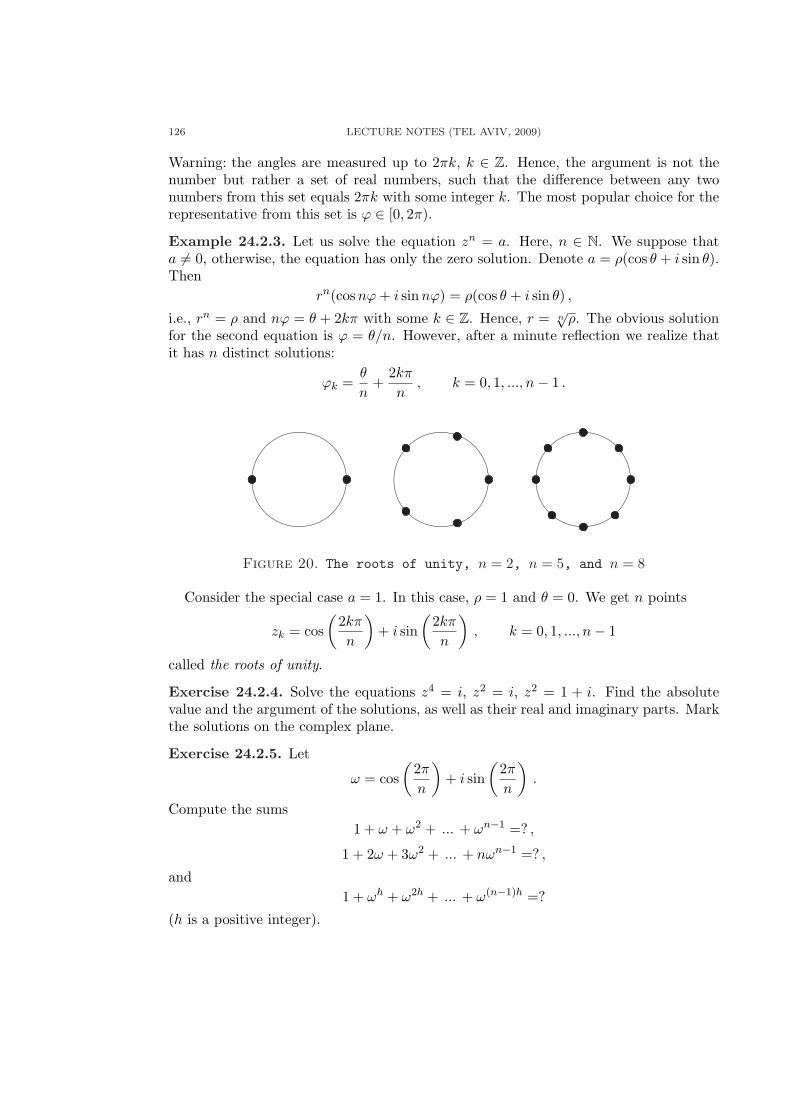
126 LECTURE NOTES (TEL AVIV, 2009)
Warning: the angles are measured up to 2πk, k ∈ Z. Hence, the argument is not thenumber but rather a set of real numbers, such that the difference between any twonumbers from this set equals 2πk with some integer k. The most popular choice for therepresentative from this set is ϕ ∈ [0, 2π).
Example 24.2.3. Let us solve the equation zn = a. Here, n ∈ N. We suppose thata 6= 0, otherwise, the equation has only the zero solution. Denote a = ρ(cos θ + i sin θ).Then
rn(cosnϕ + i sinnϕ) = ρ(cos θ + i sin θ) ,
i.e., rn = ρ and nϕ = θ + 2kπ with some k ∈ Z. Hence, r = n√
ρ. The obvious solutionfor the second equation is ϕ = θ/n. However, after a minute reflection we realize thatit has n distinct solutions:
ϕk =θ
n+
2kπ
n, k = 0, 1, ..., n− 1 .
Figure 20. The roots of unity, n = 2, n = 5, and n = 8
Consider the special case a = 1. In this case, ρ = 1 and θ = 0. We get n points
zk = cos(
2kπ
n
)+ i sin
(2kπ
n
), k = 0, 1, ..., n− 1
called the roots of unity.
Exercise 24.2.4. Solve the equations z4 = i, z2 = i, z2 = 1 + i. Find the absolutevalue and the argument of the solutions, as well as their real and imaginary parts. Markthe solutions on the complex plane.
Exercise 24.2.5. Let
ω = cos(
2π
n
)+ i sin
(2π
n
).
Compute the sums1 + ω + ω2 + ... + ωn−1 =? ,
1 + 2ω + 3ω2 + ... + nωn−1 =? ,
and1 + ωh + ω2h + ... + ω(n−1)h =?
(h is a positive integer).

DIFFERENTIAL AND INTEGRAL CALCULUS, I 127
24.3. Convergence in C. The distance between the complex numbers z1 and z2 is|z1 − z2|.Definition 24.3.1. The sequence zn converges to z (denoted by zn → z or z = lim
n→∞ zn),
if limn→∞ |z − zn| = 0.
Since
max|x− xn|, |y − yn|
≤√
(x− xn)2 + (y − yn)2︸ ︷︷ ︸=|z−zn|
≤ |x− xn|+ |y − yn| ,
the sequence zn converges to z iff the corresponding real and imaginary parts converge:
xn → x , yn → y .
Exercise 24.3.2. Check that the Cauchy criterion of convergence works for the complexsequences.
Definition 24.3.3 (continuity). The complex valued function f is continuous at z, iffor each sequence zn → z, f(zn) → f(z).
Exercise 24.3.4. Check that the sum and the product of continuous functions is con-tinuous. Check that the quotient of continuous functions is continuous in the pointswhere the denominator does not vanish.Hint: the proofs are the same as in the real case.
We see that the polynomials are continuous functions in the whole complex plane.That’s all we need to prove in the next lecture the fundamental theorem of algebra.
Exercise 24.3.5. If f = u + iv, then f is continuous iff its real and imaginary parts uand v are continuous. If f is continuous, then |f | is also continuous.

128 LECTURE NOTES (TEL AVIV, 2009)
25. The fundamental theorem of algebra and its corollaries
25.1. The theorem and its proof.
Theorem 25.1.1. Any polynomial P (z) = c0 + c1z + ... + cnzn of positive degree hasat least one zero in C.
Proof: WLOG, we assume that cn = 1. Denote m = infz∈C
|P (z)|.
Claim 25.1.2. There is a sufficiently big R such that |P (z)| > m + 1 for |z| > R.
Indeed, we have
P (z) = zn(1 +
cn−1
z+ ... +
c0
zn
),
whence
|P (z)| ≥ |z|n(1−
∣∣∣cn−1
z+ ... +
c0
zn
∣∣∣)
≥ |z|n(1−
( |cn−1||z| + ... +
|c0||z|n
)
︸ ︷︷ ︸≤1/2
)≥ 1
2|z|n
|z|≥R
≥ 12Rn ≥ m + 1
provided that R is sufficiently big. 2
Therefore, m = inf|z|≤R
|P (z)|. Next, using the Bolzano-Weierstrass lemma, we will
check that the infimum is actually attained:
Claim 25.1.3. There exists z0 with |z0| ≤ R such that |P (z0)| = m.
Indeed, choose a sequence of points zk, |zk| ≤ R, such that
|P (zk)| ≤ m +1k
.
The sequences xk = Re zk and yk = Im zk are bounded max|xk|, |yk| ≤ R. Hence, theyhave convergent subsequences. Hence, the sequence zk has a convergent subsequencezkj → z0. Then by continuity of the polynomial P , we have
P (z0) = limj→∞
P (zkj ) ,
whence |P (z0)| = m. 2
Suppose that P does not have zeroes in C, i.e., m > 0, and consider the polynomial
Q(z) def=P (z + z0)
P (z0).
Then 1 = Q(0) ≤ |Q(z)|, z ∈ C.To complete the proof, we show that there are points z where |Q(z)| < Q(0). This
will lead to the contradiction. We have
Q(z) = 1 + qkzk + qk+1z
k+1 + ... + qnzn with |qk| 6= 0.

DIFFERENTIAL AND INTEGRAL CALCULUS, I 129
Set ψ = arg qk and consider the points z with arg z =π − ψ
k. Then
arg(qkzk) = ψ + (π − ψ) = π,
so that qkzk = −rk|qk|. Let’s estimate |Q(z)| assuming on each step that r is chosen
sufficiently small:
|Q(z)| ≤∣∣∣1 + qkz
k∣∣∣ + |qk+1|rk+1 + ... + |qn|rn
= 1− rk|qk|+ rk+1|qk+1|+ ... + rn|qn|= 1− rk
(|qk| − r|qk+1| − ... − rn−k|qn|
)< 1 ,
and we are done! 2
25.2. Factoring the polynomials. In Lecture 16, we discussed the Horner schemeof the polynomial division. This scheme also works for the polynomials with complexcoefficients. It yields, that if P is a polynomial of degree n ≥ 1, then
P (z) = (z − a)P1(z) + P (a)
where P1 is a polynomial of degree n− 1. In particular, if P vanishes at a, then
P (z) = (z − a)P1(z) .
Using induction with respect to the degree of P , we arrive at
Corollary 25.2.1 (factorization of polynomials). Every polynomial of degree n ≥ 1 canbe factored:
P (z) = c(z − z1) ... (z − zn) .
Note that some of the zeroes z1,...,zn of P may coincide. We say that a is a zero ofP of multiplicity k if
P (z) = (z − a)kP1(z)
where the polynomial P1 does not vanish at a. Usually, we count zeroes of the polynomi-als with their multiplicities6. Then we can write down the factorization in the followingform
P (z) = c(z − z1)k1 ... (z − zm)km
where the zeroes z1, ..., zm are pairwise different, and∑
kj = n.
Exercise 25.2.2. If a polynomial of degree P has more than n zeroes in C (countingwith the multiplicities), then it vanishes identically.
6For instance, the polynomial P (z) = z(z − 1)2(z − 2)10 has 1 zero at the origin, 2 zeroes at z = 1,and 10 zeroes at z = 2.

130 LECTURE NOTES (TEL AVIV, 2009)
25.3. Rational functions. Partial fraction decomposition. Rational functionsare functions represented as the quotients of the polynomials:
R(z) =P (z)Q(z)
.
Writing this representation we assume that the polynomials P and Q have no commonzeroes. Then deg R
def= maxdeg P, deg Q. The rational functions form a field withusual addition and multiplication.
The rational function R is defined everywhere except of the zeroes of Q. The zeroesof the polynomial Q are called the poles of R. Note that a is a pole of R if and only if
limz→a
|R(z)| = +∞ .
If a is a zero of Q of multiplicity k, then we say that the pole of R at a also hasmultiplicity k. The polynomials are the rational functions without poles.
Claim 25.3.1. If a is a pole of R of multiplicity, then there are the unique coefficientsA1, ..., Ak such that
R(z)−(
A1
z − a+ ... +
Ak
(z − a)k
)
has no pole at a.
The sum on the RHS is called the singular part of R at a. We denote it by Sa(z).
Proof:
i (existence): Consider the rational function U(z) = (z − a)kR(z), it has no pole at a.We set Ak = U(a). Then
(z − a)kR(z)−Ak = U(z)−Ak = (z − a)V (z)
where V is a rational function without pole at a, or
R(z)− Ak
(z − a)k=
V (z)(z − a)k−1
and the RHS has a pole at a of multiplicity k − 1 or less. Then we apply the sameprocedure to the function V .
ii (uniqueness): Suppose that the expression
R(z)−(
B1
z − a+ ... +
Bk
(z − a)k
)
also has no pole at a. Then the difference of the two expressions
F (z) =B1 −A1
z − a+ ... +
Bk −Ak
(z − a)k

DIFFERENTIAL AND INTEGRAL CALCULUS, I 131
also has no pole at a. Suppose that some Al 6= Bl and set j = maxl : Al 6= Bl. Then
F (z) =1
(z − a)j
(Bj −Aj) + (Bj−1 −Aj−1(z − a) + ... + (B1 −A1)(z − a)j−1
︸ ︷︷ ︸
=T (z)
=T (z)
(z − a)j
where T is a polynomials, and T (a) = Bj −Aj 6= 0 by our assumption. Hence, F has apole at a, arriving at the contradiction. Hence, the claim. 2
Applying the claim, one by one, to all poles of R, we get
Theorem 25.3.2 (partial fraction decomposition). Every rational function R can beuniquely represented in the following form:
R(z) =∑
a
Sa(z) + W (z)
where the sum is taken over the set of all poles a of R, Saj are the corresponding singularparts, and W is a polynomial.
Exercise 25.3.3. If R = PQ where the polynomials P and Q has no common zeroes,
then deg W = deg P − deg Q, if the latter is non-negative; otherwise W = 0.
Example 25.3.4. Let
R(z) =z4 + 1
z(z + 1)(z + 2).
This function has simple poles at the points z = 0, −1, −2. Hence,
R(z) =A0
z+
A−1
z + 1+
A−2
z + 2+ W (z)
where W is a (linear) polynomial. We have
A0 = limz→0
R(z)z = limz→0
z4 + 1(z + 1)(z + 2)
=12
,
A−1 = limz→−1
R(z)(z + 1) = limz→−1
z4 + 1z(z + 2)
= −2 ,
A−2 = limz→−2
R(z)z = limz→−2
z4 + 1z(z + 1)
=172
,
and
W (z) =z4 + 1
z(z + 1)(z + 2)−
(12z− 2
z + 1+
172(z + 2)
)= ... = z − 3 ,
and finallyz4 + 1
z(z + 1)(z + 2)=
12z− 2
z + 1+
172(z + 2)
+ z − 3 .
There a more simple way to compute the linear polynomial W (z) = az + b:
a = limz→∞
R(z)z
= 1 ,

132 LECTURE NOTES (TEL AVIV, 2009)
and
b = limz→∞ (R(z)− z) = lim
z→∞z4 + 1− z2(z + 1)(z + 2)
z(z + 1)(z + 2)= −3 .
25.3.1. Simple poles and Lagrange interpolation. If the poles of R are simple (i.e., havemultiplicity 1), then we get a representation of R as a sum of simple fractions and apolynomial:
(25.3.5) R(z) =∑
j
Aj
z − aj+ W (z) .
In this case7,
Aj = limz→aj
R(z)(z − aj) = limz→aj
P (z)(z − aj)Q(z)
=P (aj)Q′(aj)
,
and we getP (z)Q(z)
=∑
j
P (aj)(z − aj)Q′(aj)
+ W (z)
where the sum is taken over the zeroes of the polynomial Q. If deg P < deg Q, then Wis zero, and we arrive at the Lagrange interpolation formula with nodes at the zeroes ofQ proven in Lecture 15.
P (z) =∑
j
P (aj)Q(z)(z − aj)Q′(aj)
.
That is, Lagrange interpolation formula is a special case of the partial fraction decom-position of rational functions!
7Here we use the derivative of the polynomial Q at a ∈ C. It is defined as usual:
Q′(a) = limz→a
Q(z)−Q(a)
z − a.
It is easy to see that this limit always exists. If
Q(z) =∑
0≤j≤n
qjzj ,
thenQ′(a) =
∑
0≤j≤n−1
(j + 1)qj+1aj .
In algebra, the latter relation is considered as a definition of the derivative Q′

DIFFERENTIAL AND INTEGRAL CALCULUS, I 133
26. Complex exponential function
26.1. Absolutely convergent series. Here we deal with absolutely convergent series∑ak with complex terms ak.
26.1.1. Rearrangement of the series. Let us recall that a series∑
a′k is a rearrangementof the series
∑ak if every term in the first series appears exactly once in the second
and conversely. In other words, there is a bijection p : N→ N such that a′k = ap(k).
Theorem 26.1.1 (Dirichlet). If the series∑
ak is absolutely convergent, then all itsrearrangements converge to the same sum.
We’ve already proved this theorem for series with real terms (Theorem 9.2.2). Forseries with complex terms the proof is the same. We observe that
ak = αk + iβk = α+k − α−k + iβ+
k − iβ−k(here we’ve used notation x+ = maxx, 0, x− = max−x, 0). Hence, we can representthe series
∑ak by a linear combination of four convergent series with non-negative
terms: ∑ak =
∑α+
k −∑
α−k + i∑
β+k − i
∑β−k .
Since all rearrangements of the series with positive terms converge to the same sum, theresult follows. 2.
26.1.2. Multiplication of series. Having two absolutely convergent series
(A)∑
k
ak
and
(B)∑
l
bl ,
we want to learn how to multiply them. Intuitively, the product (AB) should be adouble sum
(AB)∑
k,l
akbl .
The first question is how to understand this expression? The second question is does itconverges to the product A ·B?
Consider the two-dimensional array of all possible products akbl:
a1b1 a1b2 a1b3 ... a1bn ...a2b1 a2b2 a2b3 ... a2bn ...a3b1 a3b2 a3b3 ... a3bn ...... ... ... ... ... ...... ... ... ... ... ...
amb1 amb2 amb3 ... ambn ...... ... ... ... ... ...
Recall that we know how enumerate the elements of this array by the naturals N andeach enumeration leads to a different series. Luckily, the previous theorem tells us, that

134 LECTURE NOTES (TEL AVIV, 2009)
if the series we get in this way are absolutely convergent, then different enumerationswill lead to the same answer, so we’ll be able to choose the most convenient one.
Absolute convergence: observe that we can bound the finite sums
|ak1bl1 |+ ... + |aksbls | ≤(|a1|+ ... + |an|
)(|b1|+ ... + |bn|)
with n = maxk1, ..., ks, l1, ..., ls. Hence, an arbitrary finite sum |ak1bl1 |+ ... +|aksbls | isbounded by
(∑ |ak|)(∑ |bl|
). Therefore, for any rearrangement of the terms, the series
(AB) is absolutely convergent, and its sum does not depend on the rearrangement.
Cauchy’s product: the most popular rearrangement is the one called Cauchy’s product:
a1b1 + (a1b2 + a2b1) + (a1b3 + a2b2 + a3b1) + ... ,
or ∞∑
k,l=1
akbl =∞∑
n=1
∑
k+l=n
akbl =∞∑
n=1
n∑
k=1
akbn−k .
Here is our chief example:
Example 26.1.2. Suppose we have two absolutely convergent Taylor series∞∑
k=0
akzk ,
∞∑
l=0
blzl .
Then their product is represented by another absolutely convergent Taylor series∞∑
k=0
akzk ·
∞∑
l=0
blzl =
∞∑
n=0
cnzn
withcn =
∑
k+l=n
akbl .
26.2. The complex exponent. Define the functions
ez def=∞∑
n=0
zn
n!, sin z
def=∞∑
n=0
(−1)n z2n+1
(2n + 1)!, cos z
def=∞∑
n=0
(−1)n z2n
(2n)!.
First, note that the series on the RHS absolutely converge at any point z ∈ C, and thatfor real z’s the new definitions coincide with the ones we know. Now, the miracle comes:
Claim 26.2.1 (Euler).
eiz = cos z + i sin z , z ∈ C .
Proof: by inspection. We have
eiz =∞∑
n=0
(iz)n
n!=
∞∑
m=0
i2m=(−1)m
︷ ︸︸ ︷(iz)2m
(2m)!+
∞∑
m=0
i2m+1=i(−1)n
︷ ︸︸ ︷(iz)2m+1
(2m + 1)!
=∞∑
m=0
(−1)m z2m
(2m)!+ i
∞∑
m=0
(−1)m z2m+1
(2m + 1)!= cos z + i sin z .

DIFFERENTIAL AND INTEGRAL CALCULUS, I 135
Done! 2
Note that the cosine function is even, while the sine function is odd. Hence,
Corollary 26.2.2. cos z =eiz + e−iz
2, sin z =
eiz − e−iz
2i.
Corollary 26.2.3. Any non-zero complex number z can be represented in the formz = reiϕ where r = |z|, and ϕ = arg z.
Corollary 26.2.4. e2πi = 1.
Corollary 26.2.5 (Euler’s formula). eiπ = −1.
This miraculous identity connects the numbers e = limn→∞(1 + 1
n
)n, π defined asthe quotient of the length of the circumference to its diameter, and i =
√−1.
Exercise 26.2.6. Define
sinh zdef=
∞∑
n=0
z2n+1
(2n + 1)!, cosh z
def=∞∑
n=0
z2n
(2n)!.
Check the following relations:
i. cosh z =ez + e−z
2, sinh z =
ez − e−z
2.
ii. sin(iz) = i sinh z, cos(iz) = cosh z.iii. sin2 z + cos2 z = 1, cosh2 z − sinh2 = 1.
iv. sin(π
2− z
)= cos z.
The fundamental properties of the exponential function ex on the real axis are thefunctional equation ex+y = ex · ey and the differential equation (ex)′ = ex. As we know,each of these properties characterizes the exponential function. Now, we’ll check thatthis two properties persist for the function ez on C.
Claim 26.2.7. ez+w = ez · ew.
Proof: by inspection.
ez · ew =∞∑
n=0
∑
k+l=n
zk
k!· wl
l!
=∞∑
n=0
n∑
k=0
zk
k!· wn−k
(n− k)!
=∞∑
n=0
1n!
n∑
k=0
(n
k
)zkwn−k
=∞∑
n=0
(z + w)n
n!= ez+w
and we are done. 2

136 LECTURE NOTES (TEL AVIV, 2009)
Corollary 26.2.8. ez+2πi = ez; i.e., ez is a periodic function with the period 2πi.
The function f : C → C is said to be (complex) differentiable at the point z if thereexists the limit
f ′(z) = limC3ε→0
f(z + ε)− f(z)ε
.
It is important that the limit does not depend on the direction at which ε approaches0.
Claim 26.2.9. The function ez is differentiable in C and (ez)′ = ez.
Proof: We haveez+ε − ez
ε= ez eε − 1
ε.
Note that ∣∣∣∣eε − 1
ε− 1
∣∣∣∣ ≤∞∑
n=1
|ε|n(n + 1)!
= o(1)
as ε → 0. Done! 2
Related Documents


![infi2 (2) - University of Haifacs.haifa.ac.il/~dkeren/hedva/infi2.pdf · Title: Microsoft PowerPoint - infi2 (2) [Compatibility Mode] Author: dkeren-inpir Created Date: 11/18/2014](https://static.cupdf.com/doc/110x72/60e341352f6193439d68a358/infi2-2-university-of-dkerenhedvainfi2pdf-title-microsoft-powerpoint-.jpg)


