HEDG Working Paper 10/01 - University of York · HEDG Working Paper 10/01 Models For Health Care Andrew M Jones January 2010 york.ac.uk/res/herc/hedgwp

HEDG Working Paper 10/01

Models For Health Care

Andrew M Jones

January 2010

york.ac.uk/res/herc/hedgwp

MODELS FOR HEALTH CARE

ANDREW M. JONES

University of York

AbstractThis chapter reviews the econometric methods that are used by health economists tomodel health care costs. These methods are used for prediction, projection andforecasting, in the context of risk adjustment, resource allocation, technologyassessment and policy evaluation. The chapter reviews the literature on thecomparative performance of the methods, especially in the context of forecastingindividual health care costs, and concludes with an empirical case study.

Acknowledgements: I gratefully acknowledge funding from the Economic andSocial Research Council (ESRC) under the Large Grant Scheme, reference RES-060-25-0045. I am especially grateful to Will Manning for his detailed reading andextensive comments and for advice and access to Stata code from Anirban Basu,Partha Deb, Donna Gilleskie, Edward Norton and Nigel Rice.

Contents1. Introduction2. Linear regression models

2.1 Cost regressions2.2 Regression on transformations of costs

3. Nonlinear regression models3.1 Exponential conditional mean models3.2 Poisson regression3.3 Hazard models

4. Generalized linear models4.1 Basic approach4.2 Extended estimating equations

5. Other nonlinear models5.1 Finite mixture models5.2 The discrete conditional density estimator

6. Comparing model performance6.1 Evidence from the literature

7. An empirical application8. Further reading

References

1

1. Introduction

Health care costs pose particular challenges for econometric modelling. Individual-level data on medical expenditures or costs of treatment typically feature a spike atzero and a strongly skewed distribution with a heavy right-hand tail. This non-normality stems from the fact that, due to clinical complications and comorbidities,the more severe patients may attract substantial and costly services. Relatively rareevents and medical procedures might be very expensive, creating outliers in the right-hand tail of the distribution. Often, a small minority of patients are responsible for ahigh proportion of health care costs and mean costs are well above median costs. Ineconometric models of costs the error term will typically exhibit a high degree ofheteroskedasticity, reflecting both the process driving costs and heterogeneity acrosspatients1. The relationship between costs and covariates may not be linear and theappropriate regression specification for such data may be nonlinear.

When the cost data represent the population as a whole, rather than just the users ofhealth care, the distribution will typically have a large mass point at zero (with coststruncated at zero). The presence of a substantial proportion of zeros in the data hastypically been handled by using a two-part model (2PM), which distinguishesbetween a binary indicator, used to model the probability of any costs, and aconditional regression model for the positive costs. An alternative approach is to usesample selection or generalised Tobit models to deal with the zeros. The relativemerits of the two approaches are discussed in Jones (2000). Binary, multinomial andcount data models for health care utilisation have been reviewed elsewhere ( see e.g.,Jones, 2000; Jones, 2007; Jones et al., 2007; Jones, 2009). The modelling of countdata for doctor visits has strong affinities with the modelling of cost data, as bothhave non-normal heavily skewed distributions, but this chapter focuses specificallyon econometric models for non-zero health care costs

Linear regression applied to the level of costs may perform poorly, due to the highdegree of skewness and excess kurtosis; OLS minimises the sum of squared residualson the cost scale and may be sensitive to extreme observations. As a result, in appliedwork costs are often transformed prior to estimation. The most commontransformation is the logarithm of y, although the square root is sometimes used aswell. More recently the literature has moved away from linear regression towardsinherently nonlinear specifications, these include generalized linear models andextensions, such as the extended estimating equations approach, as well as moresemiparametric approaches, such as finite mixture and discrete conditional densityestimators.

Econometric models for health care costs are used in many areas of health economicsand policy evaluation. Two areas where they are used frequently are risk adjustmentand cost-effectiveness analysis. Cost-effectiveness analyses tend to work with smaller

1 For example, if total costs are generated by the sum of discrete episodes of caretimes the costs of those episodes and the episodes follow a count distribution such asthe Poisson which is inherently heteroskedastic.

2

datasets and the scope for parametric modelling may be more limited (Briggs et al.,2005). In cost-effectiveness analysis, and health technology assessment in general,the emphasis is often on costs incurred over a specific episode of treatment or over awhole lifetime. This introduces the issue of right censoring of cost data and the use ofsurvival analysis.

Risk adjustment has been adopted by health care payers who use prospective ormixed reimbursement systems, such as Medicare in the United States. It is intended toaddress the incentives for providers to engage in cream skimming or dumping ofpotential patients (Van de Ven and Ellis, 2000). Risk adjustment also plays a role inthe design of formulas for equitable geographic resource allocation (see e.g., Smith etal., 2001). In both cases regression models are used to predict health care costs forindividuals or groups of patients. The specification of these models depends on theirintended use but they typically condition on sociodemographic information, includingage and gender, diagnostic indicators and controls for comorbidities such as theDiagnostic Cost Group (DCG) system (e.g., Ash et al., 2001). In risk adjustment theemphasis is on predicting the treatment costs for particular types of patient, often withvery large datasets, and these costs are typically measured over a fixed period, such asa year. Risk adjustment entails making forecasts of health care costs for individualpatients or groups of patients and is the motivation for exploring these methods here.It means that the focus is on individual level, rather than aggregate, data. Individualdata comes from two broad sources: social surveys, in particular health interviewsurveys, and routine administrative datasets.

Administrative datasets include health care provider reimbursement and claimsdatabases, and population registers of births, deaths, cancer cases, etc. (see, e.g.,Atella et al., 2006; Chalkley and Tilley, 2006; Dranove et al., 2003; Dusheiko et al.,2004; Dusheiko et al., 2006; Dusheiko et al., 2007; Farsi and Ridder, 2006; Gravelleet al., 2003; Ho, 2002; Lee and Jones, 2004; Lee and Jones, 2006; Martin et al., 2007;Propper et al., 2002; Propper et al., 2004; Propper et al., 2005; Rice et al., 2000;Seshamani and Gray, 2004). These datasets are collected for administrative purposesand may be made available to researchers. Administrative datasets will often containmillions of observations and may cover a complete population, rather than just arandom sample. As such they suffer from less unit and item non-response than surveydata. They tend to be less affected by reporting bias, but as they are collectedroutinely and on a wide scale they may be vulnerable to data input and coding errors.Administrative datasets are not designed by and for researchers, which means theymay not contain all of the variables that would be of interest to researchers, anddifferent data sources may have to be combined.

This chapter provides an outline of the methods that are typically used to modelindividual health care costs. It reviews the literature on the comparative performanceof the methods, especially in the context of forecasting individual health care costs,and concludes with an empirical case study. Section 2 begins with linear regressionon the level of costs and on transformations of costs. Section 3 moves on to nonlinearregressions that are specified in terms of an exponential conditional mean. These canbe estimated as nonlinear regressions or by exploiting their affinity with count data

3

regression and hazard models, which can provide specifications that give additionalflexibility to the distribution of costs. Many recent studies of nonlinear specificationsare embedded within the generalized linear models (GLM) framework. The languageof the GLM approach is commonplace in the statistics literature but is less used ineconometrics and is outlined in Section 4. Recent research has seen the developmentof more flexible parametric and semiparametric approaches and some of the keymethods are described in Section 5. Section 6 reviews evidence on the comparativeperformance of methods that are most commonly used to model costs and for some ofthe recent methodological innovations. This is reinforced in Section 7 which presentsan illustrative application of the methods with data from the US Medical ExpenditurePanel Study (MEPS). Section 8 suggests some further reading.

2. Linear regression models

2.1 Cost regressionsLinear regression on the level of costs (y) is a natural starting point to model healthcare costs. It is familiar and straightforward to implement. Estimation by least squaresis easy and fast to compute in standard software even when there are hundreds ofregressors and millions of observations, which is often the case of risk adjustmentmodels based on administrative data. The model is specified on the “natural” costscale, measured directly as costs in dollars, pounds, etc., and no prior transformationis required. As the natural cost scale is used the effects of covariates (x) are on thesame scale and are easy to compute and interpret:

The model can be estimated by ordinary least squares (OLS) and predictions of theconditional mean of costs are given by:

The specification of the regression model can be checked using a variety ofdiagnostic tests. These are presented here in the context of the linear cost regressionmodel but can be extended to models for transformed costs and to the nonlinearregression models presented below.

With individual level data on medical costs there will typically be a high degree ofheteroskedasticity in the distribution of the error term, as indicated by relevantdiagnostic tests (Breusch-Pagan, 1979; Godfrey, 1978; Koenker, 1981; White, 1980).The norm is to estimate the model using robust standard errors and use these forinference (White, 1980).

A Ramsey (1969) RESET test, based on re-running the regression with squares andother powers of the fitted values included as auxiliary variables, is often used as a testfor the reliability of the model specification. In the health economics literaturePregibon’s (1980) link test is widely used as an alternative to the RESET, this addsthe level of the fitted values rather than including the individual regressors. For the

i i iy x

ˆˆ( )i ix x

4

nonlinear models discussed below the RESET and link tests may be augmented by amodified Hosmer-Lemeshow (1980, 1995) test and its variants. The idea here is tocompute the fitted values and prediction errors for the model, on the raw cost scale.These prediction errors can then be regressed on the fitted values, testing whether theslope equals zero. In the modified Hosmer-Lemeshow test an F statistic is used to testfor equality of the mean of the prediction errors over, say, deciles of the fitted values,often accompanied by a graphical residual-fitted value plot of the relationship on thecost scale. This can be implemented by regressing the prediction errors on binaryindicators for the deciles of the fitted values and testing the joint significance of thecoefficients.

A potential downside of heavily parameterized models is that they may over-fit aparticular sample of data and perform poorly in terms of out-of-sample forecasts.When models are to be used for prediction, the Copas test provides a useful guide toout-of-sample performance and guards against over-fitting (Copas, 1983; Blough etal., 1999). The Copas test works by randomly splitting the data into an estimation, ortraining, sample and a forecast, or holdout, sample (see e.g., Buntin and Zaslavsky,2004). The model is estimated on the former and used to form predictions on thelatter. The predictions from the forecast data are then regressed on actual costs to testwhether the coefficient on the predictions is significantly different from 1 overmultiple replications of the random sampling. Evidence of a significant differencesuggests a problem of over-fitting 2 . It should be noted that the tests for modelspecification - such as the RESET, link and Copas tests – are sensitive to the presenceof outliers in the data and diagnostics for influential observations should be checked,particularly when split sample tests are used (Basu and Manning, 2009).

2.2 Regression on transformed costsAs health care cost data involves working with non-normal distributions on the rawscale, for both costs and for the model residuals, much of the early literature focusedon transforming the cost data to produce a more symmetric distribution (see e.g.,Carroll and Rupert, 1988; Manning, 1998; Manning et al., 2005; Mullahy, 1998).The most popular transformation is the log transformation but square-roottransformations and other power functions are applied as well. The distinctive featureof the transformation approach is that the regression model is specified on thetransformed scale and that the model no longer works with the raw cost scale.

2 Split sample methods, such as balanced half samples, are inefficient, as only aportion of the data is used for estimation. A related approach is v-fold, or leave v out,cross validation; for each subset of v observations in the data the model is estimatedwith n-v observations and used to predict the v observations. Setting v=1, the leaveone out approach, means estimating the model n times which may be computationallyexpensive. Ellis and Mookin (2008) propose an efficient Jacknife style variant of theCopas test which makes better use of the data than the conventional 50:50 split and,in the context of the classical linear model, avoids the need to estimate the modelmultiple times.

5

Log transformationsUsing a logarithmic transformation of cost data typically reduces skewness, makingthe distribution more symmetric and closer to normality. This has lead to widespreaduse of regression models for the log of costs. One of the problems with this approachis that it requires arbitrary additional transformations if there are zero observations orthe use of two-part specifications to deal with the zeros. More importantly standardregression estimates provide predicted costs on the log scale, while analysts typicallywant results that are expressed in terms of actual costs. Simple exponentiation of thepredictions does not result in predictions on the original cost scale. To deal with thisproblem it is necessary to apply a smearing factor which is not always straightforwardto implement. This weakens the case for working with transformed data and, inparticular, problems arise with the retransformation if there is heteroskedasticity inthe data on the transformed scale (Manning, 1998; Manning and Mullahy, 2001;Mullahy, 1998).

The log regression model takes the form:

The error term is assumed to have the standard properties:

Interest lies in predicting costs on the original scale and, given E(ln(y))ln(E(y)), thisrelies on retransforming to give3:

Then:

If the error term is normally distributed, with variance , then it is possible toestimate the conditional mean for the log-normal distribution using the OLS estimatesof β and σ:

If the error term is not normally distributed, but is homoskedastic, then the estimatebased on log-normality will be biased. Instead the Duan (1983) smearing estimatorcan be applied. In this case the conditional mean is estimated using:

where is the estimated smearing factor:

where n is the sample size and k is the number of parameters in the regression.Typically this smearing factor lies between 1.5 and 4.0 in empirical applications withhealth care costs, illustrating the fact that ignoring the retransformation can lead tosubstantial underestimation of average costs.

3 Basu et al., (2006) refer to the ‘scale of interest’ and the ‘scale of estimation’.

0E 0E x

ln( )i i iy x

2

2ˆˆ ˆ( ) exp 0.5i ix x

ˆˆˆ ( ) expi ix x

1 ˆˆ ˆ ˆ1 exp , lni i i ii

n k y x

exp( ) exp( )exp( )i i i i iy x x

( | ) exp( ) (exp( ) | )i i i i iE y x x E x

6

If the error term on the log scale is heteroskedastic, Duan’s homoskedastic smearingestimator will lead to bias, with the bias being a function of x. In the lognormal case:

In the general case:

This shows that eliminating bias in the predictions requires knowledge of the form ofheteroskedasticity. This may be manageable if there are a limited number of binaryregressors. For example, the approach adopted in the RAND Health InsuranceExperiment was to split the sample by discrete x variables and apply separatesmearing estimates (see e.g. Manning et al., 1987b). In general, this is difficult if thenumber of regressors is large and contains continuous variables. However, it ispossible to exploit the fact that:

This suggests running a regression of the exponentiated residuals on x and using thefitted values as the smearing factor4. An alternative is to use separate smearing factorsfor different ranges of predicted costs, for example Buntin et al., (2004) use a separatesmearing factor for the top decile. Ai and Norton (2000) provide standard errors forthe retransformed estimates when there is heteroskedasticity.

Square root transformationsSquare-root transformations have been favoured over log transformations in someapplications. In this case the implied model is:

The smearing estimator can be adapted to the square root transformation to giveestimates of the conditional mean:

The smearing factor, assuming homoskedastic errors, is:

In the heteroskedastic case predictions take the form:

Here the smearing factor can be estimated by running a regression of the squaredresiduals on functions of x, such as the fitted values of the linear index.

Box-Cox modelsRather than imposing a particular transformation, a Box-Cox transformation can beused to specify the cost regression (see Box and Cox 1964; Chaze 2005):

4 Veazie et al., (2003) adopt a variant of this approach using the fitted values of thelinear index in place of x in the context of a square root transformation.

2ˆˆ ˆ( ) exp 0.5i i ix x x

ˆˆ( ) expi i ix x x

i i iy x

2

ˆˆˆ( )i ix x

1 2ˆ ii

N

2

ˆˆ( )i i ix x x

( ) 1ii i i

yy x

[exp( ) | ]i i ix E x

7

This includes levels (λ=1) and logs (λ=0) as special cases. Assuming has a normaldistribution, λ can be estimated, along with the other parameters, by maximum likelihood estimation in packages such as Stata (more general models are alsoavailable that apply the Box-Cox transformation to the covariates as well).Retransformation of predictions to the cost scale is not straightforward, especially inthe presence of heteroskedasticity. A more satisfactory use of the Box-Coxtransformation is provided by the Extended Estimating Equations (EEE) approachthat is discussed in Section 4 below.

Semiparametric transformation modelsThe flexibility of the Box-Cox transformation is taken a step further, whilemaintaining the idea of writing transformed costs as a linear function of the regressors,in a recent papers by Welsh and Zhou (2006) and Zhou et al. (2009). For example,Zhou et al. (2009) propose a semiparametric transformation model:

The specification is semiparametric in two senses: the transformation H(.) is treatedas an unknown increasing function and the error (0,1) has an unknown distribution.The function σ(.) captures heteroskedasticity and is assumed to be a known function. Estimation is based on an iterative algorithm that cycles between estimating β and γ, given H(.), and estimation of H(.) by nonparametric regression, given β and γ. Predictions are derived from an extended version of Duan’s (1983) smearingestimator:

3. Nonlinear regression models

3.1 Exponential Conditional Mean modelsThe transformation approach discussed above deals with the non-normality of costsby finding a transformation that makes the outcome more symmetric and thenestimating a linear regression on that scale. But these models can perform poorly andcreate the problem of retransforming predictions back to an economically meaningfulscale. To avoid this problem, the exponential conditional mean (ECM) modelassumes a nonlinear relationship for the cost regression, such that:

The ECM model is written in a general form here, to encompass specifications wherethe conditional mean is proportional to the exponential function. The use of theexponential function recognises that the object of interest, health care costs, is a non-negative quantity and accommodates the typical skewed shape of the distribution.Notice also that this implies that the effect of covariates is proportional rather thanadditive, with a constant proportional effect (see e.g., Gilleskie and Mroz, 2004).

| expi i i iE y x x

( ) ( )i i i iH y x x

1

1

ˆˆ ( )1 ˆˆ ˆˆ( ) ( )ˆ( )

ni i

i i ii i

H y xx H x x

n x

8

The ECM, and related extensions, can be estimated in a variety of ways. In practicethis is done using nonlinear least squares (NLS); the Poisson quasi-maximumlikelihood (QML) estimator; and using hazard models (for example, based onexponential, Weibull and generalized gamma distributions). Also, the ECM is closelyrelated to generalized linear models (GLMs), which are covered in Section 4.

The ECM can be viewed as a nonlinear regression model:

This can be estimated by nonlinear least squares (NLLS) or, more generally, by thegeneralized method of moments (GMM). The relevant first-order/moment conditionsare solved iteratively to give estimates of the regression parameters:

As this approach only uses the first moment rather than the full probabilitydistribution, it may be more robust than maximum likelihood, but it may also be lessefficient, depending on the form of the variance function.

3.2 Poisson regressionThe basic model used for integer-valued count data is the Poisson model. This model,and extensions such as the negative binomial model, are often used in healtheconomics to model the number of visits to a doctor but the models can also beapplied to continuous measures of health care costs (see e.g., Jones, 2000).

In the Poisson model the dependent variable yi is assumed to follow a Poissondistribution, with mean i, defined as a function of the covariates xi. Thus, the modelis defined by the distribution:

where the conditional mean i is specified by:

So the Poisson model has the ECM form and standard software designed for Poissonregression can be used to estimate the β parameters by maximum likelihood, even if the dependent variable is not an integer count, as in the case of the skeweddistribution of health care costs. The quasi-maximum likelihood (QML) property ofthe Poisson estimator means that, so long as the mean is correctly specified, it isconsistent even if higher moments, such as the conditional variance, are misspecified.In this case robust standard errors, computed using the sandwich estimator, are usedin place of the standard ML estimates.

3.3 Hazard modelsThe ECM and its extensions can be estimated using standard estimation routines forparametric hazard models. These models are normally applied to duration data but, as

exp 0i i ii y x x

| expi i i iE y x x

( )!

i iyi

ii

eP y

y

| expi i iE y x x

9

with count data regressions, can also be used for health care costs (see e.g., Jones,2000).

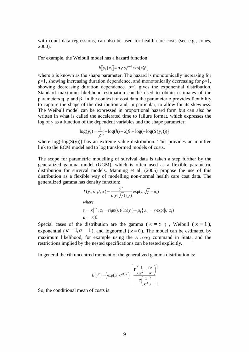
For example, the Weibull model has a hazard function:

where ρ is known as the shape parameter. The hazard is monotonically increasing for ρ>1, showing increasing duration dependence, and monotonically decreasing for ρ<1, showing decreasing duration dependence. ρ=1 gives the exponential distribution.Standard maximum likelihood estimation can be used to obtain estimates of theparameters η, ρ and . In the context of cost data the parameter ρ provides flexibility to capture the shape of the distribution and, in particular, to allow for its skewness.The Weibull model can be expressed in proportional hazard form but can also bewritten in what is called the accelerated time to failure format, which expresses thelog of y as a function of the dependent variables and the shape parameter:

1

log( ) log( ) log( log( ( )))i i iy h x S y

where log(-log(S(y))) has an extreme value distribution. This provides an intuitivelink to the ECM model and to log transformed models of costs.

The scope for parametric modelling of survival data is taken a step further by thegeneralized gamma model (GGM), which is often used as a flexible parametricdistribution for survival models. Manning et al. (2005) propose the use of thisdistribution as a flexible way of modelling non-normal health care cost data. Thegeneralized gamma has density function:

2

( ; , , ) exp( )( )

, ( ) ln( ) , exp( )

i i i

i

i i i i i

i i

f y z uy

where

z sign y u z

x

Special cases of the distribution are the gamma ( ) , Weibull ( 1 ),

exponential ( 1, 1 ), and lognormal ( 0 ). The model can be estimated by

maximum likelihood, for example using the streg command in Stata, and therestrictions implied by the nested specifications can be tested explicitly.

In general the rth uncentred moment of the generalized gamma distribution is:

2

2

2

1

( ) exp( )1

rr

r

E y

So, the conditional mean of costs is:

1| . expi i i ih y x y x

10

22

2

1

( | ) exp( ) exp( )1

i i i i iE y x x x

This shows that the model fits within the ECM class, with the mean proportional toan exponential function5. It also highlights the form of the various special cases aswell. For example, for the Weibull ( 1 ) :

1( | ) exp( ) (1 ) exp( ) 1i i i iE y x x x

For the Gamma distribution ( ):

22

2

11

( | ) exp( ) exp( )1

i i i i iE y x x x

The conditional variance of the generalized gamma model (and of the standardgamma) is proportional to the square of the mean.

Manning et al. (2005) propose that, when there is evidence that κ is small (<0.1), it is better to use a specification with additional heteroskedasticity, generated by assuming

exp( )iz for a set of regressors z. This ensures that the special cases of the

GGM, such as the lognormal model, allow for heteroskedasticity through σ.

The use of hazard models is taken further by Basu et al. (2004) who compare log-transformed models for health care costs to the semiparametric Cox (1972)

5 There is a link here with the generalized beta of the second kind (GB2) distribution.This has been used to model the size distribution of earnings and in analyses ofincome inequality and it nests other distributions such as the Burr-Singh-Maddala(BSM) and Dagum, among others (see for example, Parker, 1999; Jenkins, 2009).Mullahy (2009) discusses the issue of heavy tailed distributions and the use of theBSM distribution but the GB2 distribution does not seem to have been applied tohealth care costs. The mean of the GB2 distribution is:

1 1

( )

p qa a

E y bp q

Using exp ib x and treating the other parameters as scalars puts this in the ECM

class of models. The Burr-Singh-Maddala distribution is a special case when p=1, theDagum is a special case when q=1 and p=q=1 gives the log-logistic. Also, thegeneralized gamma, and hence the gamma and Weibull, are limiting cases of theGB2.

11

proportional hazard model. In the Cox model the hazard function at y for individual iis:

Cox’s method is described as being semiparametric because it does not specify thebaseline hazard function ho(y). Estimation uses the partial log-likelihood function,

where lRi are those observations in the risk set, Ri, at the point of exit of individual i.

By conditioning on the risk set the baseline hazard ho(y) is factored out of the partial

likelihood function. A drawback of the Cox model for modelling costs is thatestimates of the baseline hazard are required to estimate the conditional mean. But themodel does provide a benchmark for testing the ‘proportional hazards’ assumptionthat is implicit in the choice of an ECM specification.

6. Generalized linear models

6.1 Basic approachThe dominant approach to modelling health care costs in the recent literature has beenthe use of generalized linear models (see e.g., Blough et al 1999; Buntin andZaslavsky, 2004; Manning and Mullahy, 2001; Manning et al., 2005; Manning, 2006).Generalized linear models (GLMs) specify the conditional mean function directly:

For example, with an exponential conditional mean (ECM) or ‘log link’:

The first component of a GLM model is a link function g(.) that relates theconditional mean to the covariates:

The second component is a distribution (D) that belongs to the linear exponentialfamily. This is used to specify the relationship between the variance and the mean:

Advantages of the GLM approach are that predictions are made on the raw cost scale,so that no retransformation is required, and that they allow for heteroskedasticitythrough the choice of distributional family, albeit limited to specifications of theconditional variance that are pre-specified functions of the mean.

The link function specifies the shape of the conditional mean function. The mostcommonly used link functions are the identity – where covariates act additively onmean, so that the interpretation of coefficients is the same as linear regression – and

|i i i iE y x f x

| expi i i iE y x f x x

1

( )

( ) ( )

i i

i i i

g x

g x f x

( | ) ( )i i iVar y x

0| ( ) expi i i ih y x h y x

log exp( )ii li l RLogL x x

12

the log link – where covariates act multiplicatively on mean. The link functioncharacterises how the mean on the raw cost scale is related to the set of covariates.For example, with a log link:

and:

The chosen distribution is used to describe the relationship between the variance andconditional mean. Often this is specified as a power function:

Common distributional families based on the power function include:– Gaussian: constant variance; υ=0 – Poisson: variance proportional to the mean; υ=1 – Gamma: variance proportional to the square of the mean; υ=2 – Inverse Gaussian: variance proportional to cube of the mean; υ=3

Other common distributions within the GLM framework use a quadratic function of

the mean, in particular the Bernoulli, (1 ) , and binomial, (1 )n .

These distributions allow considerable flexibility in modelling cost data, although themodelling of the variance is restricted to being a specified function of the mean. Notethat the Gaussian distribution with an identity link function is comparable to linearregression. The distribution and link functions can be combined freely, although thereare canonical links for each distribution. The most popular specification of the GLMfor health care costs has been the log-link with a gamma error (Blough et al., 1999;Manning and Mullahy, 2001; Manning et al., 2005).

Estimation of GLMs is based on the classical “estimating equations” or quasi-scorefunctions:

( )0

( ) ( )

ii i i ii i

i i

ry

where r is the Pearson or standardized residual and 1

( )

i

i

are the standardized

regressors (see, Wedderburn, 1974). GLMs are based on the linear exponential familyof distributions:

This means they have the pseudo- or quasi-ML property and estimates are consistentso long as the mean is correctly specified (Gourieroux et al., 1984)6. The estimatoronly specifies the conditional mean and variance functions, so more efficient

6 Cantoni and Ronchetti (2006) propose a robust variant of GLM that modifies thequasi-score equations to make the estimator less sensitive to outliers.

| expi i iE y x x

ln |i i iE y x x

var | |i i i iy x E y x

exp( ( ) ( ) ( ) )LEFf a b y c y

13

estimators may be obtained that make use of correctly specified functions for highermoments, such as the skewness of the distribution.

The LEF density presented above is what is known as the mean parameterisation ofthe density, where:

( )

( )i

aE y

c

GLMs are more typically presented in terms of the canonical parameterisation:

( )exp ( , )

( )GLM

y bf c y

a

Where:( )iE y b

The canonical link is such that :where x

For example, with the Poisson distribution:( ) exp( ), ( ) exp( ), ln( ) ln(exp( ))b b

In applications the choice of link function and distribution is often guided by the useof the Pregibon link test, modified versions of Park’s (1966) test for the distribution,and by the use of residual plots. The link test has been described above. In the contextof GLMs it should be applied using the same link function and distribution as themodel being tested, taking care to check for influential observations in the data. Theidea of the modified Park test is that the GLM distribution should reflect therelationship between the variance and the mean, when this is based on a powerfunction it implies:

The test exploits this by regressing 2ˆln ( )i iy y on ˆln iy and a constant, typically

using a GLM to estimate the model, having tested for the appropriate form of the linkfunction to use (e.g., Manning and Mullahy, 2001). The estimated slope coefficientfrom the modified Park test provides guidance on the appropriate distributionalfamily.

4.2 Extended estimating equationsIn response to the problem of selecting the appropriate link and variance functions,Basu and Rathouz (2005) suggest a flexible semiparametric extension of the GLMmodel. Their model, which is labelled the extended estimating equations (EEE)approach, uses a Box-Cox transformation for the link function:

This includes the log-link as a special case along with other power functions of y.

This is combined with a general power function for the variance:

ln var | ln lnii iy x

1( | )i

i i i ix where E y x

21var( | )i i iy x

14

which gives a flexible specification that nests the common GLM distributions andallows the restrictions to be tested7. The additional parameters are estimated, alongwith the regression coefficients, by QML using the extended estimating equations.The EEE specification is heavily parameterized and care may be needed in calibratingnumerical optimisation routines to estimate the model8. Basu et al. (2006) apply theEEE method to claims data on the incremental costs associated with heart failure.

5. Other nonlinear models

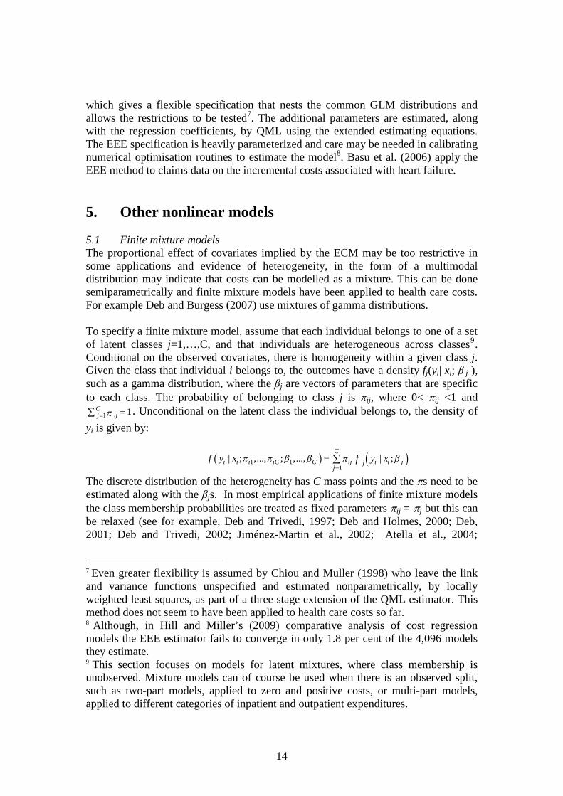
5.1 Finite mixture modelsThe proportional effect of covariates implied by the ECM may be too restrictive insome applications and evidence of heterogeneity, in the form of a multimodaldistribution may indicate that costs can be modelled as a mixture. This can be donesemiparametrically and finite mixture models have been applied to health care costs.For example Deb and Burgess (2007) use mixtures of gamma distributions.

To specify a finite mixture model, assume that each individual belongs to one of a setof latent classes j=1,…,C, and that individuals are heterogeneous across classes9.Conditional on the observed covariates, there is homogeneity within a given class j.Given the class that individual i belongs to, the outcomes have a density fj(yi| xi; β j ),such as a gamma distribution, where the βj are vectors of parameters that are specificto each class. The probability of belonging to class j is ij, where 0< ij <1 and

1 1Cijj . Unconditional on the latent class the individual belongs to, the density of

yi is given by:

1 11

| ; ,..., ; ,..., | ;C

i i i iC C ij i i jjj

f y x y xf

The discrete distribution of the heterogeneity has C mass points and the s need to beestimated along with the βjs. In most empirical applications of finite mixture modelsthe class membership probabilities are treated as fixed parameters ij = j but this canbe relaxed (see for example, Deb and Trivedi, 1997; Deb and Holmes, 2000; Deb,2001; Deb and Trivedi, 2002; Jiménez-Martin et al., 2002; Atella et al., 2004;

7 Even greater flexibility is assumed by Chiou and Muller (1998) who leave the linkand variance functions unspecified and estimated nonparametrically, by locallyweighted least squares, as part of a three stage extension of the QML estimator. Thismethod does not seem to have been applied to health care costs so far.8 Although, in Hill and Miller’s (2009) comparative analysis of cost regressionmodels the EEE estimator fails to converge in only 1.8 per cent of the 4,096 modelsthey estimate.9 This section focuses on models for latent mixtures, where class membership isunobserved. Mixture models can of course be used when there is an observed split,such as two-part models, applied to zero and positive costs, or multi-part models,applied to different categories of inpatient and outpatient expenditures.

15

Conway and Deb, 2005; Bago d'Uva, 2006). After estimating the model, it is possibleto calculate the posterior probability that each individual belongs to a given class. Theposterior probability of membership of class j depends on the relative contribution ofthat class to the individual’s likelihood function. This is given by:

1

| ;

| ;

ij j i i j

C

ik k i i kk

f y xP i j

f y x

Each individual can then be assigned to the class that has the highest posteriorprobability for them and the predicted costs can be calculated separately for eachclass.

5.2 The discrete conditional density estimatorGilleskie and Mroz (2004) propose a semiparametric approach that divides the datainto a fixed number of discrete intervals then applies discrete hazard models,implemented as a sequence of logits, to estimate the conditional density function.From that the conditional mean and other conditional expectations can be formed.This approach can be seen as a generalisation of the two-part model into a multi-partmodel: in which a separate estimate of the conditional mean is used for each of theintervals and the probability of costs lying in each interval is a function of thecovariates.

The approach begins by dividing the support of y into a fixed number (K) of discreteintervals, or bins; these may be chosen to contain an equal number of observations,such as deciles, or they may reflect features of the distribution such as a mass point atzero. The estimator focuses on an approximation to the conditional expectation ofsome function of costs h(y). This takes the form of a weighted average:

*1( ) | ( ) ( | ) ( ) [ | ]i i i i i k k ikE h y x h y f y x dy h k p y Y y x

where h*(k) is an approximation of the function of interest within the kth interval.The general formulation of the conditional expectation nests the conditional mean ofcosts, where h(.) is simply an identity. In practice, Gilleskie and Mroz (2004) chooseto use the sample mean within each interval to implement the approximation, whichdoes not allow for heterogeneity within the intervals, but local regressions could beused instead. This may be a particular problem with the open-ended interval at the topend of the distribution that contains the high cost cases (Basu and Manning, 2009)

The heart of the approach is estimation of the conditional probabilities of belongingto each interval which are then used as the weights in the averaging. They suggestthat this should be estimated by a discrete hazard specification implemented usinglogit models on an expanded version of the data. A separate logit could be estimatedfor each interval but they adopt a pooled logit model that smooths over the intervalsusing higher order polynomials in the regressors. The model is estimated for a givennumber of partitions of the support of y. To choose the appropriate number ofpartitions Gilleskie and Mroz (2004) suggest selecting the value that maximises a

16

penalised log-likelihood and, on the basis of Monte Carlo experiments, indicate that10-20 intervals will usually be sufficient. 10 Standard errors are obtained bybootstrapping the whole procedure.

6. Comparing model performance

6.1 Evidence from the literatureThere is a rich literature that compares the performance of methods of estimatinghealth care costs (see for example, Basu et al., 2004; Basu et al., 2006; Buntin andZaslavsky, 2004; Deb and Burgess 2007; Duan et al., 1983; Gilleskie and Mroz,2004; Hill and Miller 2009; Manning and Mullahy, 2001; Manning et al., 2005;Montez-Roth et al., 2006; Veazie et al., 2003). These studies include classical MonteCarlo analyses, with hypothetical cost data drawn randomly from specifiedparametric distributions, along with studies of empirical datasets that use a quasi-Monte Carlo design, with estimation and forecast samples drawn from the data. Theformer allow the performance of estimators to be assessed against known parametervalues. The latter allow the predictive performance to be assessed when the modelsare confronted with the idiosyncracies of the distribution of actual cost data, ratherthan textbook parametric distributions, although the findings may then be specific toparticular measures of costs and specific groups of people. A general finding of thesestudies is that the appropriate specification varies from application to application, forexample, depending on whether the costs relate to elderly or non-elderly patients andwhether total health care costs or specific costs such as prescription drug spending arebeing modelled. Table 1 illustrates the range of methods spanned by some recentpublished studies.

10 The estimation routine is described as being a maximum likelihood procedure butthe properties of the estimator, with respect to the sample size and number ofintervals are not derived. Although the approach is not based on explicitdistributional assumptions it does use explicit, logit, functional forms. So, comparedto some other semiparametric estimators, predictions can be computed forcounterfactual values of the regressors. This is used to compute numerical derivativesof the expected values.

17

Table 1: Coverage of methods in some recent comparative studies

Bas

u,M

annin

g&

Mull

ahy

(2004

HE

c)

Man

nin

g,B

asu

&M

ull

ahy

(2005,JH

E)

Bas

u,A

rondek

er&

Rat

houz

(2006

HE

c)

Deb

&B

urg

ess

(2007)

Hil

l&

Mil

ler

(2009,

HE

c)

OLS on y ███ ███ ███ OLS on ln(y) + Duan ███ ███ ███ ███ ███

OLS on y ███

Box-CoxGLM log-gamma ███ ███ ███ GLM linear-gamma& quadratic-gamma

███

EEE ███ ███ Weibull ███ ███ Generalized gamma ███ ███ Cox PH ███ FMM gamma ███

One of the most comprehensive published comparisons of methods is provided byHill and Miller (2009). They compare many of the models for positive expendituresthat have been discussed above: linear OLS; OLS on log costs with smearing: GLMsusing a log link and Poisson or gamma distributions; the standard generalized gammamodel (GGM), without additional heteroskedasticity, and the extended estimatingequations model (EEE). The GGM and EEE are the most flexible approaches and arenot nested within each other, but they both share the gamma model as a commonspecial case. Hill and Miller’s empirical analysis is based on the first eight waves ofthe US Medical Expenditure Panel Survey (MEPS) spanning the years 1996-2003.They regress medical expenditures on measures of chronic conditions andsocioeconomic characteristics from the previous wave of data. To encompassdifferent shapes of cost distributions the analysis uses two groups of people, elderlypeople who are eligible for Medicare and non-elderly people who have insurance, andtwo measures of costs, total health care expenditure and expenditures on prescriptiondrugs. This gives four sub-samples and the shape of the distribution of costs differsacross the samples. The comparison of models uses cross validation, in the style ofthe Copas test, with repeatedly grouped balanced half-samples (RGBHS) that takeaccount of the complex survey design of MEPS. This allows estimation andvalidation on 1024 half-samples and the models are compared in terms of model fitand out-of-sample predictions.

18

Hill and Miller’s findings echo earlier work which shows that different functionalforms (link functions) work better with different sub-samples and that it is not thecase that one specification dominates. The log link works well for total expendituresamong the non-elderly but not for the elderly. While for prescription drugs a squareroot link gives a better fit for both elderly and non-elderly. Bias is measured by themean prediction error (MPE) and predictive accuracy is measured by the meanabsolute prediction error (MAPE). The log transformed OLS model performs poorly,leading to substantial over-predictions and has the worst fit for all four distributions.The best performing models are linear OLS, Poisson regression and the EEE model.Linear OLS and EEE have less over-fitting, while the GGM and OLS on logs aremuch more likely to over-fit the data. The performance of the GGM and standardgamma model deteroriates when a log link is not appropriate, as is the case for threeout of the four empirical distributions.

The MEPS data has a relatively small sample size. In contrast Deb and Burgess(2007) make use of 3 million observations from claims data for the US Department ofVeterans Affairs (VA) for financial year 2000. This allows them to assess the role ofsample size in determining the comparative performance of different methods11. Theyuse a quasi-Monte Carlo approach, dividing the data into estimation and predictiongroups, each with 1.5m observations. The estimation group is then randomlysampled, with replacement, to give estimation samples of five different sizes rangingfrom 10,000 to 500,000. Twenty samples are generated for each sample size.Predictions are computed using the full prediction group. These are evaluated usingthe mean prediction error (MPE) that indicates overall bias; the mean absoluteprediction error (MAPE) that indicates the ability of the models to predict individualcosts; and the absolute deviations of the MAPE (ADMAPE), based on deviationsacross the experimental replications. The models control for diagnostic groups andcomorbidities and are estimated with and without trimming of the top 5 per cent ofthe cost data 12 . The results from the multiple simulations are combined andsummarised using response surface regressions.

As in Hill and Miller (2009), and other recent studies, the log regression modelperforms poorly across the board in terms of bias (MPE) and predictive accuracy(MAPE). Linear and square root regressions exhibit negligible bias on the untrimmedprediction samples. When the data is trimmed of the top 5 per cent of costs finitemixtures of gammas, with 2 or 3 components, do better than the regression models.Comparison of the different sample sizes suggests that the linear and square rootregressions converge on the asymptotic values of the MPE for sample sizes of 20-

11 Montez-Roth et al. (2006) also use VA data and compare sample sizes ranging from5,000 to 500,000, with a focus on expenditures by patients with diagnoses for mentalhealth problems and substance abuse. Their comparison of linear, square root and logmodels suggests that the square root transformation works best for predictiveaccuracy with these data.12 Note that trimming only one end of the distribution will not be mean-preserving.

19

30,000, while the finite mixture models converge with samples of 30-40k13. Whenthe focus shifts to the MAPE, the 2-component FMM dominates, whether or not thedata is trimmed. This specification also does best in terms of the DAMAPE, whichcaptures the variability across replications, but the other best performing models – thesquare root regression and the gamma model - give similar results and linear OLS isnot far behind.

7. An empirical application

To illustrate the performance of the various specifications discussed above, thissection presents an empirical application that draws on an easily accessible dataset.This is taken from Microeconometrics using Stata by Cameron and Trivedi (2009)and the dataset is available through their web page. The original source is the USMedical Expenditure Survey (MEPS), which is a set of surveys of families andindividuals, their medical providers and employers across the US. The surveys collectdata on the use of health services (e.g. frequency and cost) and whether individualshold health insurance. The particular subset of data is taken from the MEPS sampleused in Chapter 3 (p.71) of Cameron and Trivedi (2009), available as the Stata datasetmus03data.dta14. Cameron and Trivedi describe the data as follows:

“We analyze medical expenditure of individuals aged 65 years and older whoqualify for health care under the U.S. Medicare program. … Medicare does notcover all medical expenses. For example, copayments for medical services andexpenses of prescribed pharmaceutical drugs were not covered for the time periodstudies here. About half of eligible individuals therefore purchase supplementaryinsurance in the private market that provides insurance coverage against various out-of-pocket expenses.” (p71)

Total annual health care expenditures are measured in US dollars and this is theoutcome variable in the cost regressions. Sociodemographic and health-statusmeasures are also available together with insurance status. Following Cameron andTrivedi (2009) a simple additive specification of the linear index is used that includesindicators of supplementary private insurance, physical limitations, activitylimitations, the number of chronic conditions, age, gender and household income asregressors. It is important to note that the simple comparison of models presentedhear uses the same linear index in each specification. In empirical applications aricher specification will typically be used with many more covariates and withpolynomials and interaction terms, perhaps using a fully saturated model as a startingpoint if sufficient data is available (Manning et al., 1987a). A fuller and fairer

13 Note that the FMM performs poorly on the MPE criterion in the empirical casestudy presented in Section 7 which uses a much smaller sample of around 3,000observations from MEPS.14 The MEPS has a complex survey design that involves over-sampling of specificgroups. However sample weights and other design variables are not included in thissubset and, purely for the purposes of this empirical illustration, it is treated here as ifit was a simple random sample.

20

comparison of models may entail using different specifications of the regressors foreach model, so that the best specification of one model is compared with the bestspecification of another15. For example, Veazie et al. (2003) discuss the case where alinear specification, ix , is appropriate on the square root scale, then the appropriate

specification on the levels scale would be a quadratic function of ix .

The models presented here are the ones most commonly used in the health economicsliterature and some of the recent innovations: OLS estimates for linear regression ofactual costs; OLS estimates for regressions on log and square root transformations,using the Duan smearing estimator; the ECM model, estimated by NLLS and usingthe Poisson ML estimator; the generalized gamma model estimated by ML, includingthe specification with additional heteroskedasticity; the generalised beta of the secondkind (GB2); four variants of the GLM, one with a square root link and gammadistribution and three with a log link but with gamma, log-normal and Poissondistributions; the extended estimating equations model (EEE); and a finite mixturemodel (FMM) with a two-component gamma mixture. All of the models areestimated in Stata, using built-in and user-written commands16.

The sample is made up of 2,955 individuals who have positive annual medicalexpenditures (109 cases with zero costs are excluded). The mean cost is $7,290, witha minimum of $3 and a maximum of $125,610. The interquartile range of $6,064 isquite tight compared to the overall range and the distribution of costs is distinguishedby a very heavy right-hand tail. The skewness statistic is 4.1 (compared to 0 forsymmetric data) and kurtosis is 25.6 (compared to 3 for normal data). As expected forheavily skewed data, the median cost, $3334, is less than half the mean cost.

Estimates for linear regression on the level of costs show evidence of a high degree ofheteroskedasticity. For example, the Breusch Pagan test gives a F statistic of 74.1 andthe White test statistic is 104.017. Although, it is notable that the use of Huber-Whiterobust estimates does little to change the magnitude of the standard errors in thisapplication. The estimated residuals from the linear model inherit the shape of thedistribution of costs and are highly non-normal, with a skewness statistic of 4.1 and akurtosis statistic of 26.4. Individual residuals can be very large and range from -17,311 to 113,095. Also using the linear model does lead to some negative predictedcosts. Specification tests for the linear model, along with the other models, arediscussed below.

As well as making the distribution of costs more symmetric, the logarithmictransformation shrinks the range of variation in the dependent variable. When linearregression is applied to the log of costs the adjusted R2 goes from 0.11 for the levels

15 I am grateful to Will Manning for this observation.16 The discrete conditional density estimator is not included in this exercise: at thetime of writing, no standard command or user-written program for this method isavailable in the public domain.17 This is the F test version of the Breusch-Pagan statistic that drops the assumption ofnormality.

21

model to 0.23 for the log model. Heteroskedasticity is less severe than on the levelsscale but does not disappear: the Breusch-Pagan F statistic is 33.2. Using the logmodel requires retransformed estimates to predict costs 18 . The estimate of thestandard Duan smearing factor is 2.0. A similar retransformation process is applied tothe estimates of the square root regressions (see Veazie et al., 2003). The finaltransformed regression approach used here is to estimate the Box-Cox model. Thissuggests a transformation that is close to the log transformation with an estimatedvalue of λ equal to 0.076, although this estimate is statistically significantly different from 0. However this standard Box-Cox model does not allow for heteroskedasticity(unlike the EEE model).

The exponential conditional mean (ECM) model is estimated by nonlinear leastsquares (using the nl command) and Poisson regression (poisson). Extensionsthat allow for the mean to be proportional to the exponential function and capture theshape of the distribution using parametric hazard functions are estimated forexponential (streg, dist(exp)), Weibull (dist(w)) and generalized gamma(dist(gamma)) distributions. The latter can also be estimated using AnirbanBasu’s user-written code (gengam2). This provides tests of all of the nested specialcases all of which are rejected, although the lognormal distribution performs best:these are the standard gamma (chi squared equals 359.85), lognormal (16.24),Weibull (258.27) and exponential (412.52). The estimated value of κ is 0.2 and the estimate of σ is 1.19. Although the value of κ is greater than 0.1 the generalized gamma model is also estimated with additional heteroskedasticity. All of the specialcases of this variant of the model are rejected, with the lognormal again performingbest. To complement the generalized gamma model another flexible size distributionis estimated; this is the generalised beta of the second kind (GB2) which is estimatedby ML using Stephen Jenkin’s program gbfit2 (Jenkins, 2009)19.

The generalized linear model (GLM) framework is used to estimate a set of models;the first has a square root link and gamma variance (glm, link(power 0.5)family(gamma)) and the others all have log links, coupled with a gammadistribution (glm, link(log) family(gamma)), a Poisson distribution(family(poisson)), and a lognormal distribution (family(normal)). Thelink test rejects the log link but does not reject the square root link. The modified Parktests for these specifications always reject specific integer values of υ, although values of 1 (Poisson) and 2 (gamma) perform best. These GLM specifications arenested with the extended estimating equations (EEE) model of Basu and Rathouz(2005) which is estimated by Anirban Basu’s program pglm. The estimate of theBox-Cox parameter for the link function is 0.563, suggesting a square root rather thana log transformation, and the estimate of υ2 is 1.67, between the Poisson and gammadistributions.

18 The heteroskedastic smearing uses predictions from a regression of theexponentiated residuals on the fitted values of the linear index, having confirmed thatall of the predictions have positive values.19 Note that this program uses a linear rather than an exponential specification tointroduce the regressors so the version estimated here is not an ECM.

22

The finite mixture model is estimated for a two-component gamma specification,using Partha Deb’s program fmm. This divides the sample into two classes withmembership probabilities (π) of 0.75 and 0.25. The predicted costs for the first group average $2,956 and range from $694 to $23,978. While those for the second groupare higher, averaging $15,868 and ranging from $5,101 to $91,232, suggesting asmaller group of heavy users of health care.

Table 2 summarises some specification tests. P-values are reported for the Pregibonlink test (computed, where applicable, using linktest and the Pearson test, whichis related to the Hosmer-Lemeshow approach, and tests whether the correlationcoefficient between the prediction error and the fitted values, on the raw cost scale,equals 0. The Copas test is implemented by v-fold cross validation. The sample issplit into equal groups of size v and predictions for those observations are based onthe estimates of the model computed for the rest of the sample20. It is notable that theregression on log costs, the exponential conditional mean models and the glms with alog link all perform poorly according to the link test. The Copas test indicates thatboth versions of the generalized gamma specification suffer from over-fitting,although performance is improved by allowing for additional heteroskedasticity.Over-fitting seems to be less of a problem with the generalized beta of the secondkind. The GLM log-gamma model, one of the more widely used empiricalspecifications, also performs poorly with these data according to the Copas test.

Table 3 presents measures of goodness of fit within the estimation sample andmeasures of predictive performance based on the cross validation approach. For theestimation sample the measures of goodness of fit include the R2 from a regression ofactual costs on the predicted values on the raw scale, as well as the related measure ofroot mean squared error (RMSE):

and the mean absolute prediction error (MAPE):

For the cross validation estimates the RMSE and MAPE, which measure precision ofthe predictions, are augmented by the mean prediction error (MPE), which capturesbias within the forecast sample:

The three models which perform best on each criterion are highlighted in bold.

Ordinary Least Squares estimation of the linear regression model, which is based onan estimator that maximises the R-squared, does best on this specific criterion withinthe estimation sample. The EEE model and the GLM model with square root link andgamma distribution have a similar performance to OLS. The generalized gamma

20 Here the sample is split into 100 groups with either 29 or 30 observations in each group.

21 ˆni ii y y

RMSEn

1 ˆni iiMAPE abs y y

n

1 ˆni iiMPE y y

n

23

model performs worst on this criterion. The same pattern is reflected in the RMSE forboth the estimation and forecast samples. Turning attention to the MAPE, whichcaptures the precision of the predictions in terms of the level of costs, OLS no longerdominates and EEE and the GLM model do better. The finite mixture of gammasdoes even better in terms of MAPE. But this is offset by a large degree of bias in theforecast sample, indicated by the MPE. The bias is small for linear regression, thesquare root transformed regression, Poisson regression (ML and GLM) and the EEEmodel. The bias is substantial for the log transformed regression, the generalized betaof the second kind and the FMM.

The results illustrate that there may be a trade-off between bias and precision offorecasts, most starkly in the case of the FMM estimator. It is notable that the simplelinear model, estimated by OLS, performs quite well across all of the criteria, afinding that has been reinforced for larger datasets than the one used here.

24

Table 2: Specification Tests

Link testp value,withinsample

Pearsontestp value,withinsample

Copastest,v-foldcrossvalidation

OLS on y 0.133 0.974(0.608)

OLS on ln(y) 0.000 0.000 0.528(0.000)

OLS on y 0.712 0.855 1.210(0.001)

ECM - NLLS - 0.350 1.002(0.968)

ECM – Poisson-ML 0.000 0.158 0.897(0.035)

Generalized gamma 0.000 0.000 0.590(0.000)

Gen gamma + het 0.000 0.004 0.841(0.013)

Generalized beta 2 - 0.832 0.974(0.621)

GLM sqrt-gamma 0.633 0.343 0.934(0.178)

GLM log-gamma 0.000 0.000 0.759(0.000)

GLM log-normal 0.001 0.350 1.002(0.968)

GLM log-poisson 0.000 0.158 0.897(0.035)

EEE - 0.690 0.955(0.371)

FMM gamma - 0.935 0.963(0.489)

Notes:i) The results for the Copas tests with v-fold cross validation are all based on

100 groups of size 29/30. The figures reported are the slope coefficientand the p value for the test of the null hypothesis that this coefficientequals 1.

ii) Numbers in bold indicate that the model was not rejected by thespecification test at a 5% level of statistical significance.

25

Table 3: Measures of goodness of fit

R2 RMSE(1) (2)

MAPE(1) (2)

MPE

OLS on y 0.116 11270 11307 6225 6244 -1.41

OLS on ln(y) 0.095 11499 11906 6329 6639 -721.3

OLS on y 0.114 11283 11338 6181 6252 -1.12

ECM - NLLS 0.113 11296 11353 6267 6294 -102.6

ECM – Poisson-ML 0.110 11312 11362 6196 6220 -3.36

Generalized gamma 0.093 11769 11714 6429 6452 -403.5

Gen gamma + het 0.106 11354 11395 6221 6245 -39.0

Generalized beta 2 0.110 11319 11337 6409 6423 -432.1

GLM sqrt-gamma 0.115 11281 11311 6185 6203 -29.3

GLM log-gamma 0.106 11390 11432 6254 6276 -147.0

GLM log-normal 0.113 11295 11353 6267 6294 -102.6

GLM log-poisson 0.110 11312 11362 6196 6220 -3.36

EEE 0.116 11274 11310 6179 6200 -7.06

FMM gamma 0.106 11395 11433 5775 5793 1132.7

Note: R2 denotes the R-squared from a regression of actual costs on the predictedvalues; RMSE is the root mean squared prediction error, on the cost scale, where (1)is for the estimation sample and (2) is for the cross validation predictions; MAPE isthe mean absolute prediction error; MPE is the mean prediction error (bias) for thecross validation predictions.

26

8. Further reading

This chapter has focused on estimating and predicting health care costs usingregression models and microdata. A comprehensive guide to microeconometricmethods in general is provided by:

Cameron, A. C. and P. K. Trivedi (2005). Microeconometrics. Cambridge:Cambridge University Press.

This has a companion text which shows how the techniques can be implemented inStata, with many empirical examples, including the use of the MEPS data on healthcare expenditures:

Cameron, A. C. and P. K. Trivedi (2009). Microeconometrics Using Stata. CollegeStation Texas: Stata Press.

Models for health care costs are often based on health survey data. The issuesassociated with survey design, sampling, nonresponse and imputation, and inferencewith complex surveys are discussed in depth by:

Korn, E. L. and B. I. Graubard (1999). Analysis of Health Surveys. New York: JohnWiley & Sons Inc.

Parametric models for health care costs draw on the theory of size distributions suchas the lognormal and generalized gamma. These and other size distributions are givena comprehensive treatment in:

Kleiber, C. and S. Kotz (2003). Statistical Size Distributions in Economics andActuarial Sciences. New York: John Wiley & Sons Inc.

A classic text for generalized linear models is:

McCullagh, P. and J. A. Nelder (1989). Generalized Linear Models. Second Edition.Boca Raton: Chapman and Hall.

The application of GLMs in Stata is described in:

Hardin, J. W. and J. M. Hilbe (2007). Generalized Linear Models and Extensions.Second Edition. College Station Texas: Stata Press.

27

References

Ai, C. and E. C. Norton (2000). 'Standard errors for the retransformation problem withheteroscedasticity.' Journal of Health Economics, 19: 697-718.

Ash, A. S., R. P. Ellis, G. Pope, M. S. John, J. Z. Ayanian, D. W. Bates, H. Burstin, L. I.Iezzoni, E. McKay and W. Yu (2000). 'Using diagnoses to describe populations andpredict costs.' Health Care Financing Review, 21: 7-28.

Atella, V., F. Brindisi, P. Deb and F. C. Rosati (2004). 'Determinants of access tophysician services in Italy: a latent class seemingly unrelated probit approach.' HealthEconomics, 13: 657-68.

Atella, V., F. Peracchi, D. Depalo, and C. Rossetti (2006). 'Drug compliance, co-payment and health outcomes: evidence from a panel of Italian patients.' HealthEconomics, 15: 875-92.

Bago d'Uva, T. (2006). 'Latent class models for utilisation of health care.' HealthEconomics, 15: 329-43.

Basu, A., B. V. Arondekar and P. J. Rathouz (2006). 'Scale of interest versus scale ofestimation: Comparing alternative estimators for the incremental costs of acomorbidity.' Health Economics, 15: 1091-107.Basu, A. and W. G. Manning (2009). 'Issues for the next generation of health care costanalyses.' Medical Care, 47: S109-S114.

Basu, A., W. G. Manning, and J. Mullahy (2004). 'Comparing alternative models: log vsCox proportional hazard?' Health Economics, 13: 749-65.

Basu, A. and P. J. Rathouz (2005). 'Estimating marginal and incremental effects onhealth outcomes using flexible link and variance function models.' Biostatistics, 6: 93-109.

Blough, D. K., C. W. Madden and M. C. Hornbrook (1999). 'Modeling risk usinggeneralized linear models.' Journal of Health Economics, 18: 153-71.

Box, G. E. P. and D. R. Cox (1964). ‘An analysis of transformations.’ Journal of theRoyal Statistical Society B, 26: 211-252.

Breusch, T. S. and A. R. Pagan (1979). 'Simple test for heteroscedasticity and randomcoefficient variation.' Econometrica, 47: 1287-1294.

Briggs, A., R. Nixon, S. Dixon, and S. Thompson (2005). 'Parametric modelling of costdata: some simulation evidence.' Health Economics, 14: 421-28.

28

Buntin, M. B. and A. M. Zaslavsky (2004). 'Too much ado about two-part models andtransformation?: comparing methods of modeling Medicare expenditures.' Journal ofHealth Economics, 23: 525-42.

Cameron, A. C. and P. K. Trivedi (2009). Microeconometrics Using Stata. CollegeStation Texas: Stata Press.

Cantoni, E. and E. Ronchetti (2006). 'A robust approach for skewed and heavy-tailedoutcomes in the analysis of health care expenditures.' Journal of Health Economics, 25:198-213.

Carroll, R J. and D. Rupert (1988). Transformations and Weighting in Regression. NewYork: Chapman and Hall.

Chalkley, M. and C. Tilley (2006). 'Treatment intensity and provider remuneration:dentists in the British national health service.' Health Economics, 15: 933-46.

Chaze, J. P. (2005). ‘Assessing household health expenditure with Box-Cox censoringmodels.’ Health Economics, 14: 893-907.

Chiou, J-M. and H-G. Müller (1998). ‘Quasi-likelihood regression with unknown linkand variance functions.’ Journal of the American Statistical Association, 93: 1376-1387.

Conway, K. S. and P. Deb (2005). 'Is prenatal care really ineffective? Or, is the 'devil' inthe distribution?' Journal of Health Economics, 24: 489-513.

Copas, J. B. (1983). ‘Regression, prediction and shrinkage.’ Journal of the RoyalStatistical Society B, 45: 311-354.

Cox, D. R. (1972). ‘Regression models and life tables.’ Journal of the Royal StatisticalSociety B, 34: 187-200.

Deb, P. (2001). 'A discrete random effects probit model with application to the demandfor preventive care.' Health Economics, 10: 371-83.

Deb, P. and J. F. Burgess Jr. (2007). 'A quasi-experimental comparison of statisticalmodels for health care expenditures.' Mimeo.

Deb, P. and A. M. Holmes (2000). 'Estimates of use and costs of behavioural health care:a comparison of standard and finite mixture models.' Health Economics, 9: 475-89.

Deb, P. and P. K. Trivedi (1997). 'Demand for medical care by the elderly: a finitemixture approach.' Journal of Applied Econometrics, 12: 313-36.

Deb, P. and P. K. Trivedi (2002). 'The structure of demand for health care: latent classversus two-part models.' Journal of Health Economics, 21: 601-25.

29

Dranove, D., D. Kessler, M. Mcclellan, and M. Satterthwaite (2003). 'Is moreinformation better? The effects of 'report cards' on health care providers.' Journal ofPolitical Economy, 111: 555-88.

Duan, N. (1983). 'Smearing estimate: a nonparametric retransformation method.'Journal of the American Statistical Association, 78: 605-10.

Duan, N., W. G. Manning, C. N. Morris, and J. P. Newhouse (1983). 'A comparison ofalternative models for the demand for health care.' Journal of Business and EconomicStatistics, 1: 115-126.

Dusheiko, M., H. S. E. Gravelle and R. Jacobs (2004). 'The effect of practice budgetson patient waiting times: allowing for selection bias.' Health Economics, 13: 941-58.

Dusheiko, M., H. S. E. Gravelle, R. Jacobs and P. C. Smith (2006). 'The effect offinancial incentives on gatekeeping doctors: evidence from a natural experiment.'Journal of Health Economics, 25: 449-78.

Dusheiko, M., H. S. E. Gravelle, N. Yu and S. Campbell (2007). 'The impact ofbudgets for gatekeeping physicians on patient satisfaction: evidence from fundholding.'Journal of Health Economics, 26: 742 - 62.

Ellis, R. P. and P. G. Mookin (2008). 'Cross-validation methods for risk adjustmentmodels.' Mimeo, Boston University.

Farsi, M. and G. Ridder (2006). 'Estimating the out-of-hospital mortality rate usingpatient discharge data.' Health Economics, 15: 983-95.

Gilleskie, D. B. and T. A. Mroz (2004). 'A flexible approach for estimating the effectsof covariates on health expenditures.' Journal of Health Economics, 23: 391-418.

Godfrey, L. G. (1978). 'Testing for multiplicative heteroscedasticity.' Journal ofEconometrics, 8: 227-236.

Gourieroux, C. S., A. Monfort and A. Trognon (1984). ‘Pseudo maximum likelihoodmethods: theory.’ Econometrica, 52: 680-700.

Gravelle, H. S. E., M. Sutton, S. Morris, F. Windmeijer, A. Leyland, C. Dibben and M.Muirhead (2003). 'Modelling supply and demand influences on the use of health care:implications for deriving a needs based capitation formula.' Health Economics, 12: 985-1004.

Hill, S. C. and G. E. Miller (2009). ‘Health expenditure estimation and functional form:application of the generalized gamma and extended estimating equation models.’ HealthEconomics, in press, DOI: 10.1002/hec.1498.

Ho, V. (2002). 'Learning and the evolution of medical technologies: the diffusion ofcoronary angioplasty.' Journal of Health Economics, 21: 873-85.

30

Hosmer, D. W. and S. Lemeshow (1980). ‘Goodness of fit tests for the multiple logisticregression model.’ Communications in Statistics – Theory and Methods, 9: 1043-1069.

Hosmer, D. W. and S. Lemeshow (1995). Applied Logistic Regression. Second edition.New York: Wiley.

Jenkins, S. P. (2009). 'Distributionally-sensitive inequality indices and the GB2 incomedistribution.' The Review of Income and Wealth, 55: 392-398.

Jiménez-Martin, S., J. M. Labeaga and M. Martínez-Granado (2002). 'Latent classversus two-part models in the demand for physician services across the EuropeanUnion.' Health Economics, 11: 301-21.

Jones, A. M. (2000). 'Health Econometrics'. In Culyer, A. J. and J. P. Newhouse (eds),Handbook of Health Economics. Amsterdam: Elsevier.

Jones, A. M. (2007). Applied Econometrics for Health Economists: A Practical Guide.Oxford: Radcliffe Medical Publishing.

Jones, A. M. (2009). 'Panel data methods and applications to health economics'. in Mills,T. C. and K. Patterson (eds) Palgrave Handbook of Econometrics. Volume 2. London:Palgrave MacMillan.

Jones, A. M., N. Rice, T. Bago d'Uva, and S. Balia (2007). Applied Health Economics.London: Routledge.

Koenker, R. (1981). 'A note on studentizing a test for heteroscedasticity'. Journal ofEconometrics, 17: 107-112.

Lee, M.-C. and A. M. Jones (2004). 'How did dentists respond to the introduction ofglobal budgets in Taiwan? An evaluation using individual panel data.' InternationalJournal of Health Care Finance and Economics, 4: 307-26.

Lee, M.-C. and A. M. Jones (2006). 'Heterogeneity in dentists' activity in Taiwan: anapplication of quantile regression.' Empirical Economics, 31: 151-64.

Manning, W. (1998). 'The logged dependent variable, heteroscedasticity, and theretransformation problem.' Journal of Health Economics, 17: 283-95.

Manning, W. (2006). 'Dealing with skewed data on costs and expenditure.' In Jones,A.M. (ed) The Elgar Companion to Health Economics. Cheltenham: Edward Elgar.

Manning, W. G., A. Basu and J. Mullahy (2005). 'Generalized modeling approaches torisk adjustment of skewed outcomes data.' Journal of Health Economics, 24: 465-88.

31

Manning, W.G., N. Duan and W.H. Rogers (1987a). 'Monte Carlo evidence on thechoice between sample selection and two-part models.' Journal of Econometrics, 35:59-82.

Manning, W., J. P. Newhouse, N. Duan, E. Keeler, A. Leibowitz and M. S. Marquis(1987b). 'Health insurance and the demand for medical care: evidence from arandomized experiment.' American Economic Review, 77: 251-77.

Manning, W. G. and J. Mullahy (2001). 'Estimating log models: to transform or not totransform?' Journal of Health Economics, 20: 461-94.

Martin, S., N. Rice, R. Jacobs and P. C. Smith (2007). 'The market for elective surgery:joint estimation of supply and demand.' Journal of Health Economics, 26: 263 - 85

Montez-Roth, M., C. L. Christiansen, S.L. Ettner, S. Loveland and A. K. Rosen (2006).‘Performance of statistical models to predict mental health and substance abuse cost.’BMC Medical Research Methodology, 6: 53. DOI: 10.1186/1471-2288-6-53.

Mullahy, J. (1998). 'Much ado about two: reconsidering retransformation and the two-part model in health econometrics.' Journal of Health Economics, 17: 247-81.

Mullahy, J. (2009). 'Econometric modeling of health care costs and expenditures. Asurvey of analytical issues and related policy considerations.' Medical Care, 47: S104-S108.

Park, R. E. (1966). ‘Estimation with heteroscedastic error.’ Econometrica, 34: 888.

Parker, S. C. (1999). ‘The generalised beta as a model for the distribution of earnings.’Economics Letters, 62: 197-200.

Pregibon, D. (1980). ‘Goodness of link tests for generalized linear models.’ AppliedStatistics, 29: 15-24.

Propper, C., S. Burgess and K. Green (2004). 'Does competition between hospitalsimprove the quality of care: hospital death rates and the NHS internal market.' Journalof Public Economics, 88: 1247-72.

Propper, C., B. Croxson and A. Shearer (2002). 'Waiting times for hospital admissions:the impact of GP fundholding.' Journal of Health Economics, 21: 227-52.

Propper, C., J. Eachus, P. Chan, N. Pearson and G. D. Smith (2005). 'Access to healthcare resources in the UK: the case of care for arthritis.' Health Economics, 14: 391-406.

Ramsey, J. B. (1969). ‘Tests for specification errors in classical linear least squaresregression analysis.’ Journal of the Royal Statistical Society B, 31: 350-370.

32

Rice, N., P. Dixon, D. Lloyd and D. Roberts (2000). 'Derivation of a needs basedcapitation formula of allocating prescribing budgets to health authorities and primarycare groups in England: regression analysis.' British Medical Journal, 320: 284 -88.

Seshamani, M. and A. Gray (2004). 'Ageing and health care expenditure: the red herringargument revisited.' Health Economics, 13: 303-14.

Smith, P. C., N. Rice and R. Carr-Hill (2001). ‘Capitation funding in the public sector.’Journal of the Royal Statistical Society A, 164: 217-257.

Van de Ven, W. and R. P. Ellis (2000). ‘Risk adjustment in competitive health planmarkets.’ In A. J. Culyer and J. P. Newhouse (eds), Handbook of Health Economics.Amsterdam: Elsevier.

Veazie, P. J., W. G. Manning and R. L. Kane (2003). ‘Improving risk adjustment forMedicare capitated reimbursement using nonlinear models.’ Medical Care, 41: 741-752.

Wedderburn, R. W. M. (1974). ‘Quasi-likelihood functions, generalized linear models,and the Gauss-Newton method.’ Biometrika, 61: 439-447.

Welsh, A. H. and X. H. Zhou (2006). 'Estimating the retransformed mean in aheteroscedastic two-part model.' Journal of Statistical Planning and Inference, 136:860-81.

White, H. (1980). 'A heteroscedasticity-consistent covariance matrix estimator and adirect test for heteroscedasticity.' Econometrica, 48: 817-838.

Zhou, X-H. H. Lin and E. Johnson (2009). ‘Non-parametric heteroscedastictransformation models for skewed data with an application to health care costs.’ Journalof the Royal Statistical Society B, 70: 1029-1047.